Amateur Horizontal Component Seismometer, with Passive Leveling,Detects the Earth’s Free Oscillations Down to 1 mHz

(Model MkXXI)

Allan ColemanE-mail Address: adcoleman3@verizon.net

Initiated: 1 December 2005Last revised: 8 January 2006

ABSTRACT

An unorthodox horizontal component seismometer with force feedback incorporated a passive leveling method thatminimized the amount of long period (LP) tilt noise contaminating the output signal, from this amateur built instrument. Thetransfer function calculated an output signal flat to velocity between 0.011–20 Hz. Compared to a conventional horizontalseismometer, sensitivity to very long period (VLP) seismic signals was greatly enhanced in the absence of VLP tilt noise. Afterfast Fourier transforming (FFT) any time series containing 24 hours of continuous seismic velocity data, fundamentalspheroidal and toroidal modes of the earth’s free oscillations were routinely displayed with peak frequencies down to 1 mHz,the cut off point of the data processing software. One aspect of the mechanical design did not adequately prevent tilt noise fromentering the data at the top end of the frequency range, resulting in a response similar to a conventional tilt sensitive horizontalseismometer.

INTRODUCTION

A LP horizontal component seismometer based on an inertial-mass system responds simultaneously to both linearground accelerations and rotational ground tilt. As the ground tilts in a direction aligned with the seismometer’s sensitive axis, gravity will shift the pendulum’s position of equilibrium, producing a signal similar to a seismic disturbance. Severe tilting will force the instrument’s velocity or displacement transducer to drift out of range.

Some experimenters [1] [2] have used the electrical output signal of a sensitive tiltmeter to cancel the tilt signalembedded in the output of an adjacent BB or very broad band (VBB) horizontal component seismometers. Other researchersinvolved in near-field work [3] [4] post processed data collected from horizontal and vertical channels to derive separatehorizontal displacement and tilt signals. Each of the above methods required two individual instruments, potentially leading toincreased electronic noise, signal scaling and installation issues. A large non-portable piece of apparatus [5] consisting of apendulous anti-tilt platform (natural period 2.4 seconds) successfully isolated LP tilt noise from a horizontal seismometerplaced on it, but unfortunately short period sensitivity was sacrificed. To date, there appears to be no commercially availableseismometer capable of delivering a true tilt free horizontal output signal.

Why experiment with a horizontal seismometer design for VLP noise reduction? Major noise source for a verticalseismometer are barometric pressure fluctuations, which manifests itself two ways. It deforms the instrument’s enclosure/internal framework and causes a vertical pumping motion on the earth’s surface. Another problem is the gravitational influenceof the air mass above the seismic mass, which affects frequencies below 2 mHz. Ground tilt is the only major noise sourceconcerning a horizontal seismometer. It is easier to control noise from one source, than from three.

In essence, the MkXXI’sbase plate’s incessant tilting motion was somewhat de-coupled mechanically from thehorizontal pendulum’s vertical hinge.Imagine a beam tiltmeter and horizontal seismometer rolled into one unit. A portion ofthe pendulum’s supporting framework literarily floating on two equipotential surfaces, i.e. a self-leveling datum plane definedby gravity, per the principles of a long base water tiltmeter described by A. A. Michelson. In theory, most LP tilt noise shouldnot destabilize the pendulum’s equilibrium. Electronic circuits and transfer function were configured and calculated like aconventional BB horizontal seismometer.

CONSTRUCTION DETAILS

MECHANICAL

Background:Design complexity was limited to the equipment and materials on hand in the home garage. Besides a selection of

powered hand tools, more powerful machinery like a mill/drill machine, metal cutting band saw and a 3” metal lathe (hobby type) assisted with cutting and shaping of the thicker materials. Several of the MkXXI’s mechanical components were

2

modified salvaged parts from earlier homemade seismometers, which helped to keep expenses and fabrication time to aminimum. Review Figures 1-6 for further information not disclosed in this section.

Design Concept:The concept was to flexibly attach a horizontal seismometer of conventional design to a sub-plate resting on a rigid

floor slab, see Figure 1. Thedisplacement transducer’s null position was near constantly maintained, by controlling the verticalorientation ofthe pendulum’s hingeaxis in a plane vertical and parallel to the sensitive axis. Hinge axis could still be adjustedin a plane perpendicular to the sensitive axis, like a conventional horizontal design, to optimize the pendulum’s natural periodby tilting the base plate with the leveling screws.

A tee assembly comprised of: the pendulum, displacement transducer and feedback transducer were mounted on thecentral arm and a leveling float at each end of the cross arm. Tee assembly pivoted with limited movement about a pin(fulcrum point) in contact with a pedestal protruding up from the base plate, see Figure 2. Radial movement of the teeassembly, relative to the base plate, was kept in check with a flexible link between the two. Each float was partially immersedin a tank of mineral oil, with a balance tube running between the tanks. Slowly tilting the base plate, orientated with thesensitive axis, caused the oil level to lower in one tank and rise in the other, ensuring an equipotential datum plane. Floatsrigidly attached to the tee assembly, prevented transducer drift by tracking the datum plane.

Here is the theory behind the concept, as currently understood. Visualize a horizontal plane defined by three points onthe tee assembly, the center of buoyancy (CB) for each of the two floats and the pivot pin (fulcrum point) on the central arm.On that horizontal plane lies a neutral axis, around which the tee assembly rotates, running from the pivot pin to the mid-pointbetween the floats. In theory, the center of gravity (CG) of the entire tee assembly should fall on the neutral axis. If the CG isabove the neutral axis (i.e. above the CB), the tee assembly may respond like an inverted pendulum to horizontal groundaccelerations.In practice, it’s best to keep the CG a few millimeters below the neutral axis. Flexible link attached to the end ofthe neutral axis established the second hinge point for the tee assembly.

Mineral oil was selected for the leveling fluid because: it is odorless, has a high flash point and moderate viscositywith an extremely low evaporation rate. When lightly tapping on the tee assembly, viscosity of the oil quickly damped (almostcritically) any vertical oscillation. In a severe local seismic event, the oil will slosh out of the tanks and strange cross talkmodes would appear in the data.

Tee Assembly:The pendulum is a piece of 3/16” thick aluminum alloy sheet, approximately 140mm long. Mounted to it were the

inner plates of the displacement transducer carrying the modulating signal, brass seismic masses and the feedback coil. Totalequivalent seismic mass used in the transfer function was approximately 0.07 Kg, about 103mm from the pendulum’s hinge. Two pieces of 0.002” thick heat treated phosphor-bronze shim formed flexures (both in tension), connected the pendulum tothe 1/8” thick alum alloy centralarm of the assembly. Mounted on the central arm were the outer signal receiver plates of thedisplacement transducer as well as the permanent magnet (Figure 3), part of the feedback transducer. Natural period of thependulum was 3 seconds. An alum angle piece, bonded to the end of the central arm, held a short piece of a drill bit with aground conical point (pivot pin) that later engaged a dimple mark, punched in the top surface of an alum bracket fastened to thebase plate. Note: heavy items like feedback transducer magnet and seismic masses were deliberately placed over the pivot pin,so the floats had less weight to support.

Screwed to the central arm, was the 1/16” thick alum cross arm with white colored floats, actually plastic containers 65mm OD x 58mm high. Their lids were vented and fastened to the cross bar. Center distance between floats was 270mm,center of float to pivot pin 205mm, midpoint of cross arm to the pivot pin 190mm. Each float had to displace approximately0.107 Kg of mineral oil. On a conventional horizontal seismometer, leveling screws on the base plate are used to null thedisplacement transducer. After oil was added to the tanks, a small trim mass was positioned in different places on one of theMkXXI’s floats to achieve the same result. Once nulled, no further trimming was necessary.

Base Plate:A rigid base plate is very important to the overall stability of a conventional horizontal seismometer. Thermal stresses

or the unyielding weight of the pendulum can cause plate warping, thereby creating another source for tilt noise. The beauty ofutilizing a true tilt compensating design means certain structural components can be fabricated out of materials normallyclassified as unacceptable. In stead of a chunk of metal for the base plate, a scrap piece of PVC plastic plate 390 mm x 220 mmx 19 mm thick was selected. In theory, if the plastic warps slightly, the pendulum should not drift off center. Three screws withknurled knobs used in conjunction with a bull’s eye spirit level, manually leveled the plate during initial set-ups.

Flexible Link:This feature compensated for vertical and twisting motions of the tee assembly, to keep the radial position of the

sensitive axis in check horizontally. Small pieces of iron nails were bonded to a piece of 1/16” diameter brass wire see Figure4. Overall length of this assembly was 75mm. Nail tips were pointed, contacting the center of a rare earth magnet attached tothe cross arm at the neutral axis, and another one mounted on a post protruding from the base plate. Magnets had minimal

3

influence on the small iron nails, in regards to pulling them off balance. Unfortunately, it required only 25 grams to pull thenail off the magnet, but that’s OK for surviving the tug of low energy teleseismic waves.

Tanks:Each tank was fabricated from a 4” ABS pipe fitting, and capped at the bottom end. Next, each tank was bonded to an

alum sheet for attachment to the base plate. Brass barb fittings, ¼ NPT, threaded and bonded into the sides of the tanks, matedto a piece of ¼” ID Tygon tubing to carrying oil between the two tanks. An oil drain plug was added to one of the tanks. Draftcovers were made from 1/16” thick fiberglass PCB material, held up with long screws slipping into shallow holes around theperiphery of each tank.

Temporary Cross Bar Supports:Two pieces of 1/4UNC threaded rod were secured to the base plate, each having an adjustable knurled nut to

temporarily support the cross bar while the instrument was assembled, wired and calibrated. After oil was added to the tanksand the cross arm just began to float free of the nuts, they were rotated down out of the way.

Draft Cover:Re-used a 1” thick rigid Styrofoam insulation coverpreviously installed on a homemade seismometer, since it cleared

the protruding features of the seismometer by just 10 mm. Cover was fabricated from pieces of Styrofoam sheet bondedtogether to form a simple five sided box. A foam rubber gasket around the bottom edge of the cover sealed it to the floor underthe instrument.

Feedback Transducer:A voice coil, working in conjunction with a permanent magnet elevated above the base plate, applied a feedback force

proportional to ground acceleration that both modified and damped the pendulum's motion. The motor constant was kind oflow at 3.3N/A, the term Gn used in later feedback calculations. Figure 6 partially shows some of homemade transducer’s external details. A rare earth magnet salvaged from a scrapped electronic enclosure and bonded to the inside of an ironplumbing fitting used for the magnetic return path. Its voice coil gap was thoroughly cleaned by sliding pieces of vinylinsulation tape through it, capturing loose magnetic particles, flakes of paint, lint, hair and dead skin. A large piece of tape wastemporarily placed over the exposed poles and gap to prevent dirt and metallic particles from re-entering. Tape was removed atfinal assembly with the coil. The voice coil bobbin was made from pieces of PVC pipe fittings, complete with vent holes in thebulkhead, to allow the free passage of air between bobbin and magnet. A length of 36 gauge enameled magnet wire waswrapped around, and bonded to, the bobbin. Coil resistance equaled 63 ohms.

Displacement Transducer:A full bridge or symmetric differential capacitive (SDC) transducer [6] offered a well defined null position and does

not require a very precise symmetric oscillator. Its does however require two variable capacitors and a precise method fordifferentiating their output signals. An SDC transducer basically consists of two separate displacement transducers, coupledtogether to move as a single unit, with each transducer forming a branch of the bridge circuit. When responding to detectablemotion between the seismic mass and base plate, each transducer’s output was of opposite polarity to the other, providing atrue differential output signal. Viscous air trapped between the plates exited through a pattern of vent holes were uniformlydistributed across all plates of the transducer.

Fastened to the pendulum were the two inner plates (modulated signal transmitters), each one divided electrically intotwo separate active areas, facing towards the center plate. Each of the outer plate’s active areas was joined electrically to the diagonally opposite active area on the opposing outer plate. The outer plates (modulated signal receiver), mounted to thecentral arm of the tee assembly, was also divided electrically into two active areas. Whenever one of the outer plates movedcloser to the center plate, one half of the center plate received a stronger positive signal while the other half of the center platereceived a stronger negative signal. Fine 40 AWG coax wire carried the modulating signal from the oscillator circuit to theinner plates. These coaxes easily flexed where they bridged the gap at the pendulum’s hinge. The outer plate’s active areas overlapped the sides of the center plate, accommodating any slight unavoidable off-axis motions without noticeably effectingsensitivity.

The capacitor plates, inner and outer, weremade from 1/8” thick FR-4 (PCB) material coated with 1 oz, 0.0014” thick copper foil. It was assumed that the board’s manufacturer applied some type of corrosion inhibitor on the exposed coppersurface. Boards were cut to shape with a band saw and a Dremel Tool engraved isolation grooves 1-2 mm wide, defining theactive areas in the copper layers. Mounting screws and metal spacers were electrically isolated from all active areas. Outerbraided jackets of the modulating signal’s coaxes were only tied to the electronics’ metal enclosure to extend the RFI shield.Nominal gaps either side of the center plate measured 0.8 mm. Parallelism between the center and outer plates were within0.08 mm at the extremes of pendulum travel. Air viscosity was less of an issue when the total vent hole area was greater than15% of the total plate area (i.e. active area + vent hole area) for the given nominal gaps. Sensitivity was not adverselycompromised. The displacement transducer constant measured to be 190,288 V/M

4

ELECTRONICS

General:There were two separate hand-wired boards, the Displacement Transducer Circuit Board (DTCB) and the Feedback

Circuit Board (FCB). The DTCB was segregated to one aluminum project box, and the sensitive analog circuits of the FCB inanother. An off-the-shelf +/-12 VDC, dual linear supply (1 amp per side), powered the circuit boards.

Circuits were constructed using metal film resistors with 1% tolerances, for all values up to 1 meg ohm. Larger valueswere carbon types with 5% tolerances. All power decoupling caps and feedback cap values under .01 microfarad were ceramic,all others >.01 mF were polyester. The circuits were built on perforated boards with sockets for all ICs. To reduce power railnoise, the power pins on all op amps were wired via 20-Ohm resistors to a common point on the output pins of the voltageregulators. To eliminate or significantly reduce ground loops, a small piece of adhesive backed copper foil 3 mm wide by 20mm long was attached to the underside of the perf board, between the rows of legs of each op amp socket. Decoupling caps andother components associated with each op amp requiring grounding were soldered to the piece of foil. Then each individual foilwas connected directly to a common ground point on the circuit board, no daisy chaining. Also, .01 mF ceramic decouplingcaps were inserted where power-carrying wires entered a circuit board. A short length of coax cable connected the output of theDTCB to the FCB. The coax outer shield was connected to the metal project boxes. Any flux residues seen built up on thecircuit boards, extending between conductors, were scraped off as best as possible to reduce potential signal leakage.

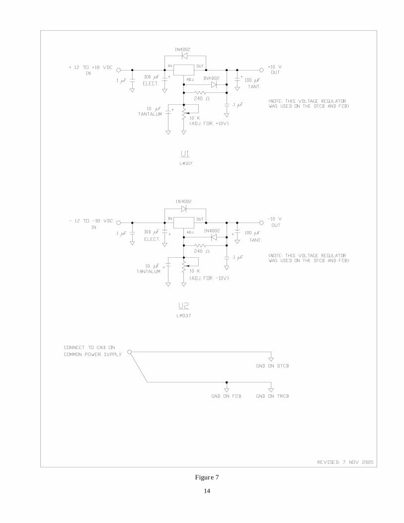
Displacement Transducer Circuit Board (DTCB):Adjustable voltage regulators U1 and U2 (Figure 7) filtered and stepped down the voltage from the common supply,

providing the circuits with +/-10 VDC. With 10 mF Tantalum capacitors connected to the regulators, better than 65dB rippleand spike rejection was possible. The IN4002 diodes protected the regulators from excess voltages during power down.

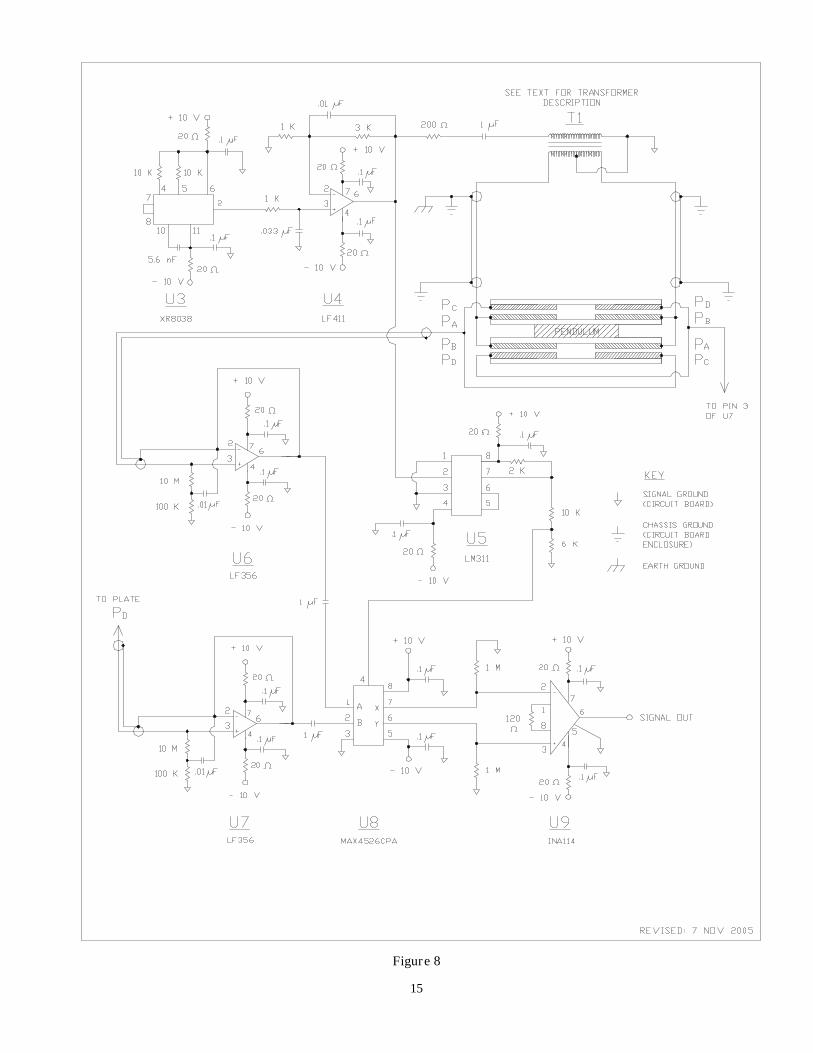
Function generator U3 (Figure 8) had a total harmonic distortion of 2-3% and similar tolerance for the frequencystability and produced a 5.4 KHz sine wave output signal. Precision DC operational amplifiers have increasing noise towardsthe lower frequencies, so operating the transducer with a reasonably high AC frequency reduced the 1/f noise problem. Sinewave was filtered and buffered by op amp U4 with a 4X gain to increase P-P value. An audio transformer T1 (Digi-Key P/N237-1121-ND) with 600-600 ohm center tapped coils were referenced to ground for DC common-mode voltage rejection. Thesecondary coils produced two modulating signals, 180 degrees out of phase with each other and connected to the active areason the SDC’s moving inner plates, PA and PB, per the diagonally opposing pattern shown in Figure 8.

Op amp U5 is a zero-crossing detector referenced to ground for converting the AC sine wave into a sharp squarewave, oscillating from 0 to +10 volts. A divider lowered the triggering voltage seen by the demodulator’s analog switch U8 to +3.8 volts max. Active areas on the capacitor’s fixed outer plates, PC and PD detected the modulated voltage signal’s amplitude and phase in proportion to the displacement of the inner plates, in either direction from their null position. High impedanceunity gain amplifiers, op amps U6 and U7, drove guards (the coax outer shield) to reduce stray input capacitance for additionalsensitivity, plus the input pins to these op amps were bootstrapped for circuit stability. Their outputs were fed into the analogswitch U8, a demodulator synchronized with the sine wave signal from U4, monitoring the modulated voltage of each halfcycle. Op amp U9, an instrumentation amplifier (IA) with 418X gain, differentiated the signal from the SDC. Coax audiocables half a meter long were soldered to the SDC, and connected to the circuit board via RCA phono plugs. The outer shieldsof the two inner plate’s coaxes were attached to chassis ground.

Feedback Circuit Board (FCB):Adjustable voltage regulators U1 and U2 (Figure 7), including their associated components were duplicated on this

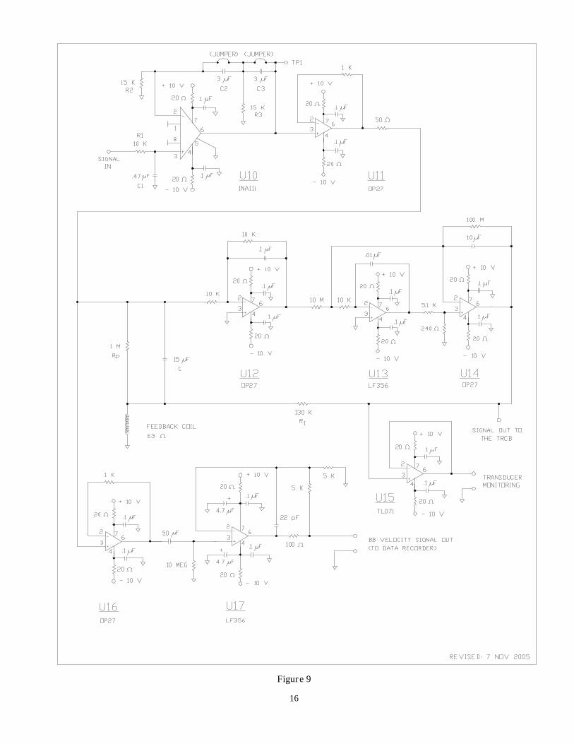
board to supply filtered +/- 10 VDC to the circuit.Referring now to Figure 9, op amp U10 is configured as a special integrator with the intended purpose of improving

low frequency sensitivity and stability. Such an “integrator” appeared in papers written by Erhard Wielandt [7][8][9], seenadjacent to the displacement transducer in block diagrams representing the electronic circuitry of Streckeisen seismometers.Erhard Wielandt, via personal communications, explained that because the system would oscillate if high gain is maintained athigh frequencies, loop gain had to be frequency-dependent, increasing towards the low frequencies while ensuring unity gain atthe higher frequencies. One way to realize this is to insert a special integrator or quasi-integrator, within the feedback loop.Based on the word description he provided and after some experimentation, a workable circuit design evolved. A 1st order 34Hz LPF attenuated high frequency circuit noise from the displacement transducer prior to entering the quasi-integrator. Op amp10 is a unity gain instrumentation amplifier (IA) with high impedance FET inputs and excellent common mode rejection(CMR) to differentiate between small input signals. A 2nd order 3.5 Hz high pass filter (HPF) comprising of C2, C3, R2 and R3was inserted into the integrator’s feedback loop between pins 2 and 6 of the IA. A buffer op amp U11 installed after theintegrator prevented any unwanted loading of downstream circuits. A temporary shunt was installed across the capacitors C2and C3 when the system was calibrated and removed later for normal operation.

The multi-path feedback circuit followed a schematic published by Sean-Thomas Morrissey for his verticalcomponent VBB seismometer, the STM-8 [10], which itself was based on similar circuits found on VBB seismometers. Multi-path feedback is a combination of differential and integral feedback signals flowing through the feedback transducer mountedon the pendulum. The differential signal dominates across the passband of interest, decreasing towards the lower frequencies

5

where the strength of the integral signal increases. Reading the papers by Morrissey and Wielandt is highly recommended fortheir discussions on this subject. Resistor Rp and capacitor C provided the proportional feedback. The combined currents ofRp, C and RI flowed through the feedback coil, modifying the pendulum motion for a BB velocity response. The capacitorsdesignated C, were a combination of Mylar caps connected in parallel.

Following the quasi-integrator, op amp U12 inverted the acceleration signal before it entered a composite integrator,comprising of U13 and U14. Composite integrators [11] take advantage of a FET op amp’shigh input impedance, combinedwith the DC output accuracy of a BJT op amp. The RC time constant of 100 seconds, the product of the 10 Meg resistor andthe 10 microfarad capacitor, is the mathematical term TI used in later calculations. Op amp U15 buffered the circuit wheneverthe displacement signal was monitored with a voltmeter. Op amp U16 buffered a1st order 0.0008 Hz (1250 seconds) high passfilter that removed unwanted DC signal drift. Finally, op amp U17 with a 2X gain, drove a capacitive load created by a 10-meter long coax cable connecting the seismometer to the data logger, a PC fitted with an internal A/D card. Not shown in theelectronic schematics was a simple 1:2 voltage divider, installed between the output of U17 and the A/D card, thus preventingit from receiving a voltage signal exceeding its rated input of +/- 5 volts.

Polarity of the Output Signal:The accepted standard is a positive voltage output signal whenever the ground moves north or east for a N-S or E-W

aligned instrument, respectively. By gently pushing the pendulum in the opposite directions, i.e. south or west, verified signalpolarity. This was equivalent to inertia holding the seismic mass stationary above the base plate. A positive voltage signalshould be present at pin 6 on U9, U15 or U17. A negative voltage signal would require the wires to pins 1 and 2 on U8 to bereversed. If this step resulted in the pendulum going into wild oscillations, reverse the wires to the feedback coil.

TRANSFER FUNCTION

System Response:The transfer function is a mathematical statement that describes the relationship between the input, a set of

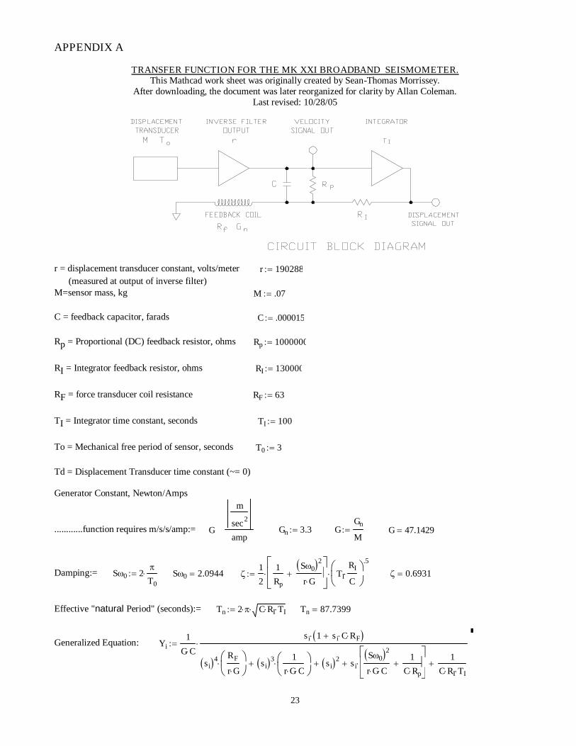
predetermined parameters, and the output of the system. Calculating a system’s output can be a very difficult task. Fortunately the MathCAD file compiled by Morrissey for his STM-8 was available for downloading [12], saving a great deal of time andeffort. MathCAD Standard 2000 software was used to open the file on a local PC. The STM-8’s values were substituted with different ones. See Appendix A at the end of this paper (the MathCAD work sheet. Numerous values were inserted for C, Rp,RI and TI, before settling on those below for an acceptable response:

Input parameters:r = 190,288 V/mM = 0.07 KgC = 0.000015 FaradsRp = 1 meg OhmsRI = 130 K OhmsGn = 3.3 Newton/AmperesRf = 63 OhmsTI = 100 secondsTo = 3.0 seconds

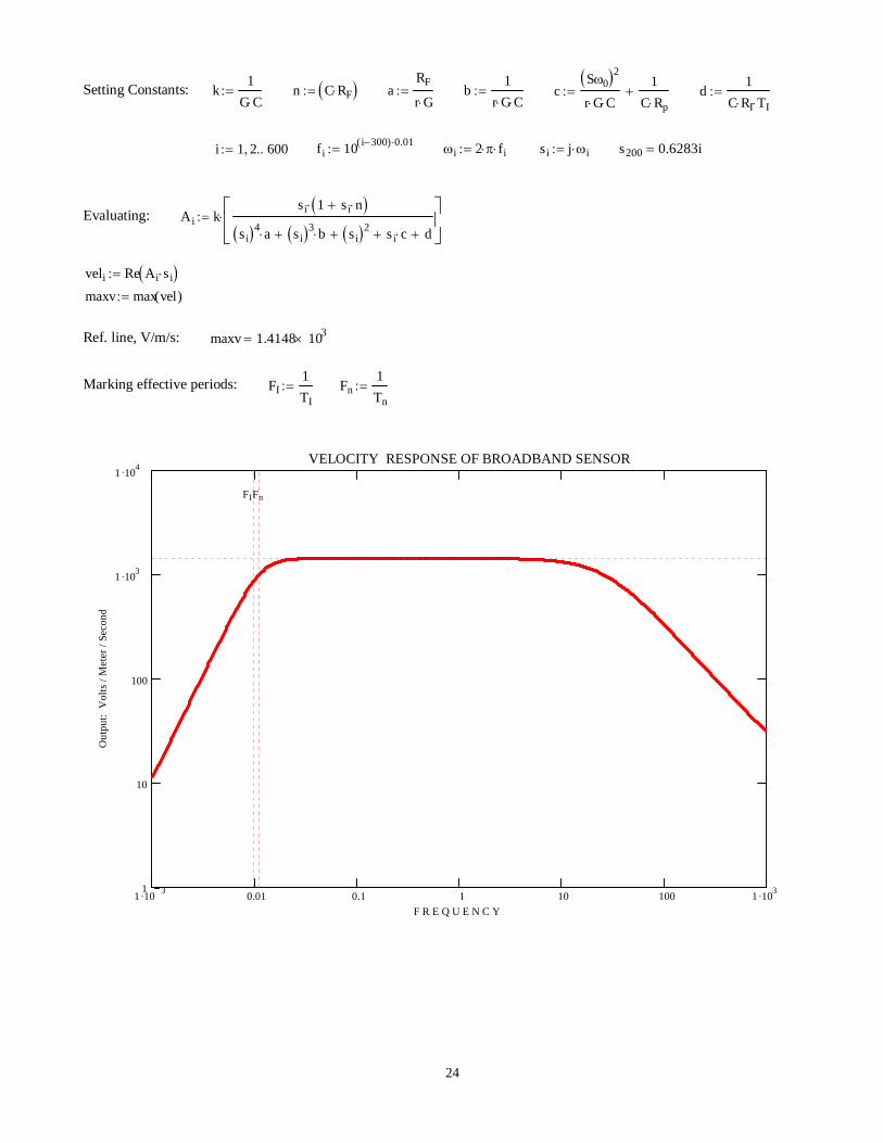
Calculated system response:Zeta = 0.70 (damping)Tn = 88 seconds (closed loop natural period)V/m/s = 1,415 (max sensitivity)The plotted curve for the velocity response showed the high frequency end rolling off at roughly 20 Hz (Appendix A), but itwas the quasi-integrator that limited the top end to about 4 Hz.

DATA PROCESSING

Output data from the seismometer was analog passband filtered 0.3-100 mHz, then collected with a 16 bit A/D card(model PSN-ADC-12/16 Rev 2 from Larry Cochrane of Redwood City, California USA) installed unshielded on themotherboard of a NEC 233 MHz Pentium desktop PC. The A/D card’s clock crystal was housed in a temperature-controlledoven and corrected by a WWV time signal.

Data collected at 50 samples per second (SPS), and displayed using Seismic Data Recorder (SDR) software, Version4.1. Seismic event files were time and date stamped by the software, re-sampled and saved in PSN format. WinQuake software,Version 2.9.8, analyzed the data files created with SDR. To produce acceptable looking seismograms, digital filters furthercontrolled passband limits and roll-offs, extracting useful seismic data from unwanted background noise. After entering theevent’s origin time and co-ordinates into WinQuake, the embedded JB Tables calculated the theoretical arrival times for P and

6

S waves, placing markers at the proper locations on the seismograms. WinQuake also performed FFT analyses on a maximumof 1439 minutes of continuously sampled velocity data. The movable software cursor had a +/- 2 seconds visual positionalaccuracywhen “picking”discrete velocity wave peaks.

VAULT LOCATION AND CONDITIONS

Seismometer co-ordinates:Latitude: 47.849 NLongitude: 122.328 WElevation: 110 metersSensitive axis alignment: E-W

The passive leveling feature was put to the ultimate test; for the entire duration of the experiment, the seismometerwas installed on the basement floor of a house, approximately 10 meters from the data logger. Each of the seismometer’s leveling feet were supported by a piece of 4” square by ¼” thick plate glass, pressing on a plastic bag spread across carpeting12-15mm thick covering the concrete floor slab. According to a geologic map, over 200+ meters of unconsolidated glacial tillseparated bedrock from the floor slab. Ambient basement temperatures, at floor level, ranged 10 - 15º C. For the entire onemonth data was collected, very favorable weather conditions prevailed. Outside wind conditions were calm, their velocitiesscarcely exceeding a few kilometers per hour.

RESULTS

Short Period:Carpeting under the seismometer reduced its high frequency sensitivity, by at least 15dB, to the 20-30 freight trains

passing by every day one kilometer away, but their passage was still very recognizable.

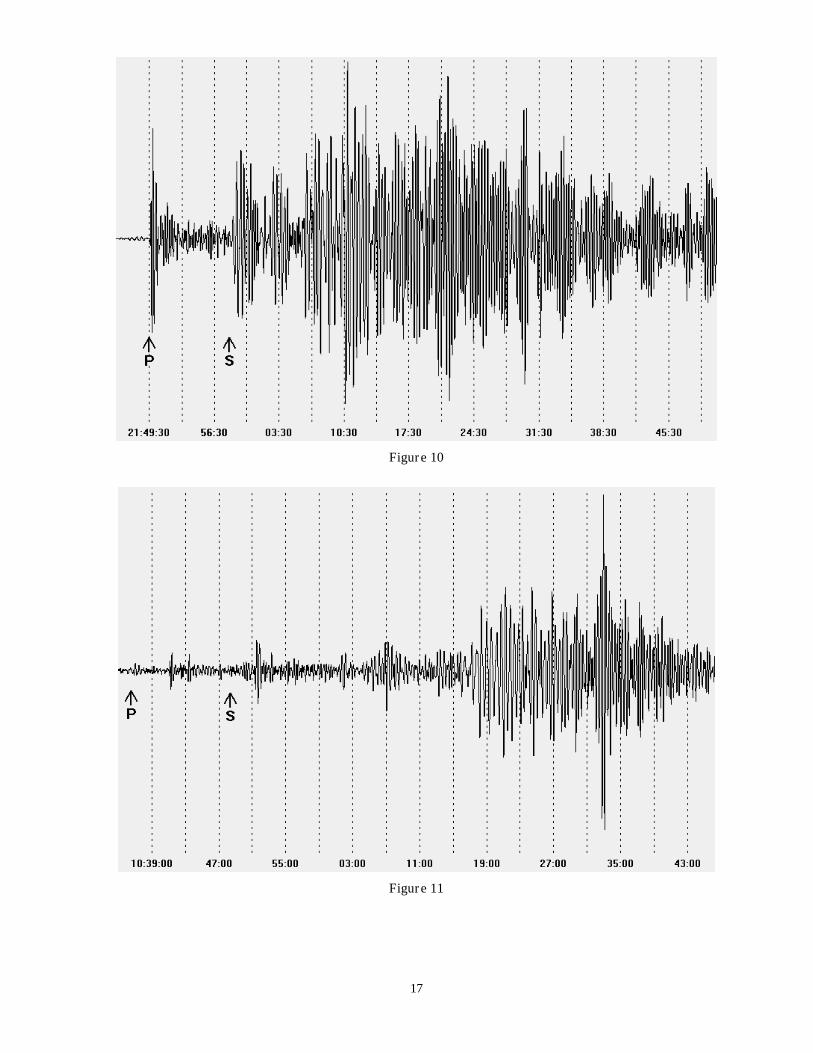
Long Period:Tilt noise was evident in the broad band data, diminishing progressively towards the lower frequencies. Seismograms

of teleseismic events (Figures 10 & 11) required narrow 0.03-0.08 Hz pass band filters to extract body and surface wavedetails. Individuals walking within 5 meters of the seismometer produced long period disturbances, recognizable in the data asrandomly placed spikes protruding out of the noise in the 1439 minute time series selected for later FFT analysis (Figures 12 &15).

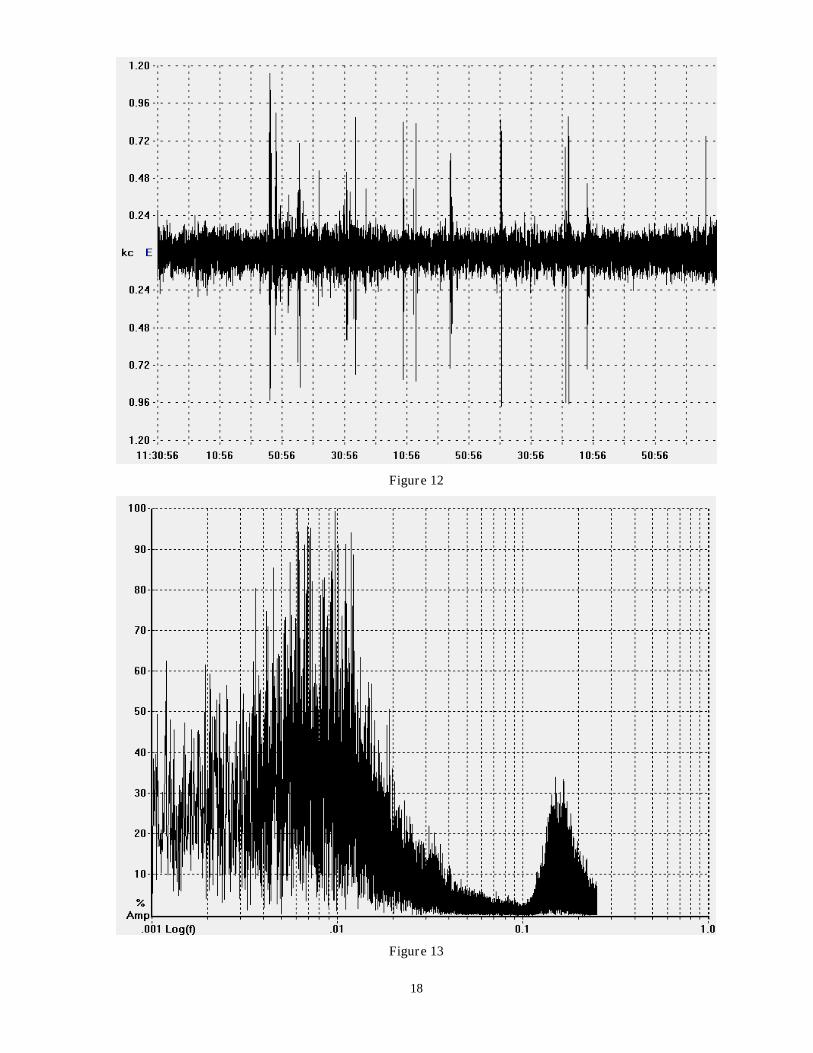
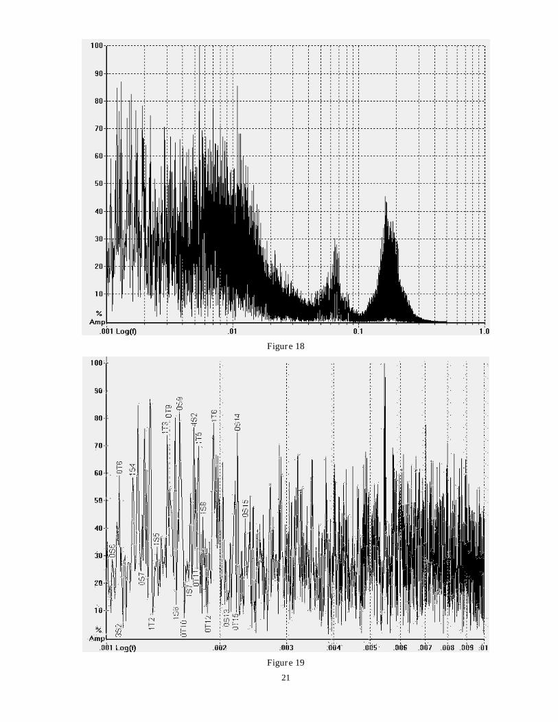
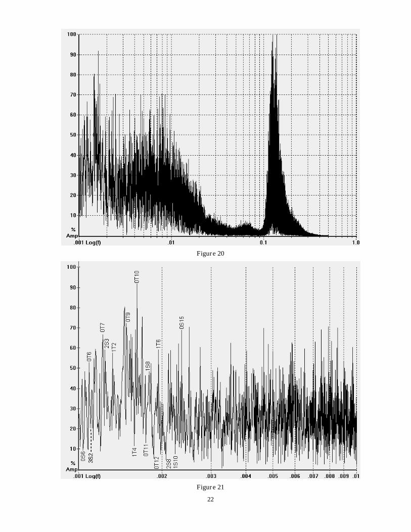
Very Long Period:Individual time sets containing 1439 minutes of continuous velocity data after fast Fourier transformation (Figures 13,

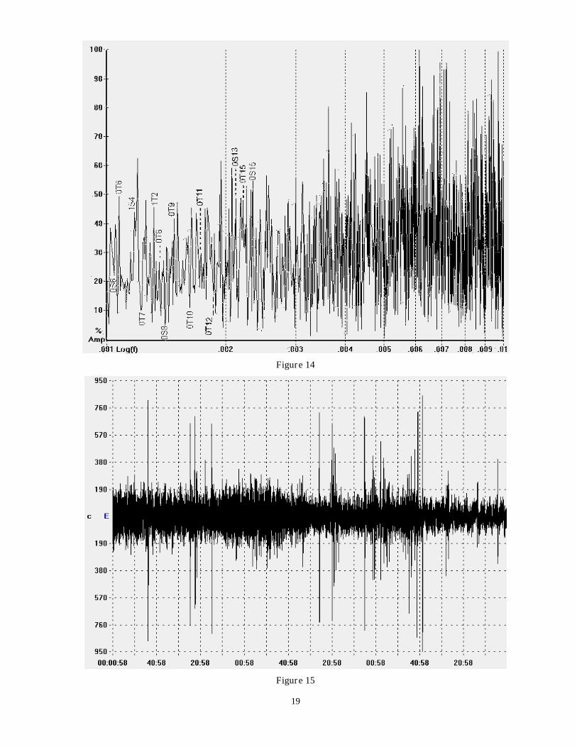
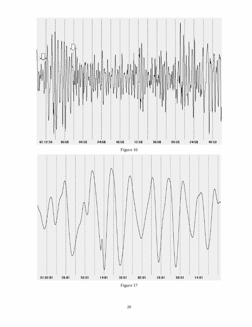
18 & 20), produced spectrums down to 1 mHz, a minimum frequency set by WinQuake. After expanding the low end of theFFT spectrum (Figures 14, 19 & 21), spheroidal and toroidal modes were very carefully picked manually and identified using apublished list [13] of frequencies centered on discrete acceleration peaks. Each expanded FFT spectrum uncovered bothfundamental and overtone modes (singlet and multiplet) of free oscillations in the 1-2 mHz band as well as the earth’s “hum” in the 2-7 mHz band. Velocity waves, 90º out of phase with acceleration, were compressed narrow enough in the spectrogramsto make picking modes straight forward. Movement of people near the seismometer, seen in the raw signal as narrow spikes,formed peaks with 1.2-1.3 mHz center frequencies. One times series, 2nd ordered low pass filtered to 0.001 Hz (Figure 16),contained waves having periods between 19-26 minutes, including a couple of suspect longer period waves. For one example,see Figure 17.

An old panel mount analog galvanometer connected to pin 6 of op amp U15 (see Figure 9) continuously monitored the“mass position”of the pendulum. Meter’s needle did not move visually (<0.1 volt) from the original set up position, afterseveral months of resting on the basement floor, proving that VLP tilt was under control.

DISCUSSION

Of course, installing the seismometer in a quiet isolated subterranean vault on solid bedrock would have achievedmore informative results. Locating the MkXXI on a basement floor simulated a real world situation for most amateurs, who areforced to operate instruments in an environment filled with tilt noise. With the glass support plates nested in the compliantcarpet fibers, the compressed fibers were very attenuative to the high frequencies, while low frequency energy found littleresistance reaching the seismometer.

Tilt noise in the LP data is thought to be caused by three things: 1) restriction of oil flow through the undersized ¼” inside diameter (ID) balance tube between the two tanks formed a mechanical low pass filter, 2) wires connecting thetransducers to electronics were suspended too far from the tee assembly’s neutral axis and 3) floats possibly effected by surfacetension of theoil’s meniscus, due to narrow gap size between float OD and tank ID. Correcting these problems by; increasing

7

balance tube ID, re-routing wires closer to the neutral axis of the central arm and increasing the ID of the tanks, should help tiltinsensitivity up to ~ 0.2 Hz using current leveling method.

All waves displayed in the 1-2 mHz band of the FFTs were initially thought to be noise, until paper plots exhibitedremarkable similarities from one time series to another. WinQuake’s cursor positional accuracy of less than +/- 0.06 % at 500seconds, ruled out the likelihood that the many measured peaks were random noise. Whether it was a seismically quiet day, orone excited by a large event (M6.8), each spectrogram presented a smorgasbord of free oscillations of varying amplitudes,mixed in with some environmental noise. Peaks were only labeled if they accurately matched a published frequency and had anadjacent open space to accommodate text. In actuality, many identified modes went unlabeled due to lack of room for the text.Processing software features were basic, could not FFT analyze more than 24 hours of data at a time, with no capability ofstacking multiple time series. Sensitive axis (E-W alignment) was pointed directly at the center of the Gulf of Alaska.Undoubtedly, late autumn storm systems churned up the atmosphere and sea to excite the free oscillations.

No measurements of seismic cross axis coupling or parasitic frequencies were attempted. Unusual seismometergeometry may have some unknown quirks that aided in the excellent VLP sensitivity. Could the pendulum be swingingsideways far enough to upset the balance, creating a behavior similar to an inverted pendulum? Probably not, when the motionis controlled with a feedback force.

CONCLUSIONS

Four weekends were spent building the seismometer with supporting electronics. The self-leveling equipotentialsurface defined a datum plane for the two floats, precise enough to control the restoring force of gravity on the pendulum atvery long periods, avoiding transducer drift. Using a fluid to level the seismometer is not messy if one is careful. Sidewaysmovement of the fluid in the holding tanks should form mini seiches during a regional or local event, thereby ruining all data.This design weakness relegates the instrument to teleseismic studies. The MkXXI was never meant to be a serious instrument,just evaluate a concept.

Direct observation of the fundamental 0S6 spherical and 0T6 toroidal modes in the FFT spectrum indicated that themechanical concept is functional and the electronic circuits were stable. Because of the process software’sinability to provide aspectrum analysis covering 0.1-1 mHz, it was impossible to know when local environmental or instrument noise finallyobscured all seismic signals. Lower modes were actually detected (Figure 16) using clumsier visual methods.

It was highly encouraging to see the horizontal capture VLP data while sitting on the carpet covered basement floor,one of the worst places imaginable to operate a sensitive seismometer. Conventional seismometers like the VBB StreckeisenSTS-1 vertical and superconducting gravimeters must be installed at the quietest vaults in the world in order to detect the 2-4mHz band, a band which occurs at the quietest section on the Peterson New Low Noise Model (NLNM). Future generations ofhorizontals, free of tilt noise, may assist those low noise verticals to locate the sources of the earth’s hum.

REFERENCES

[1] Morrissey, S-T., The Very Broadband Beam-Balance Tiltmeter. 10 December 2000. Retrieved 1 November 2005from the World Wide Web.http://www.eas.slu.edu/People/STMorrissey/abstracts.html

[2] Hutt, C.R., Holcomb, L.G., Sandoval, L.D., An Inertial Rotation Meter (Tiltmeter). 24-26 March 2004. BroadbandSeismometer Workshop Posters. Retrieved 15 March 2005 from the World Wide Web.http://www.iris.edu/stations/seisWorkshop04/PPT/Tiltmeter_Poster.ppt

[3] Wielandt, E., Forbriger, T., Near-field seismic displacement and tilt associated with the explosive activity ofStromboli. 1999. Annali di Geofisica, 42(3), 407-416. Retrieved 11 November 2005 from the World Wide Web.http://www-gpi.physik.uni-karlsruhe.de/pub/forbriger/download/paperware/tiltshort.pdf

[4] Weins, D.A., et al. Tilt recorded by a portable broadband seismograph: The 2003 eruption of Anatahan Volcano,Mariana Islands. 24 September 2005. Geophys. Res. Lett., 32, No. 18, L18035. Retrieved 11 November 2005 fromthe World Wide Web.http://epsc.wustl.edu/seismology/doug/Files/pozgay_et_al_jvgr_2005.pdf

[5] Lin’kov, E.M., Superlong-period Horizontal Seismometeric Channel. 1992. Seismicheskie Pribory, 23, 48-53[English translation: 1993. Seismic Instruments, 23, 47-52]

[6] Peters, R. D., SDC SENSORS. (no date). Retrieved 20 August 2002 from the World Wide Web.http://physics.mercer.edu/petepag/sens.htm

8

[7] Wielandt, E. and Streckeisen G., The leaf-spring seismometer: design and performance. 1982. Bull. Seism. Soc. Am.,72(6), 2349-2367.

[8] Wielandt, E. and Steim, J. M., A digital very-broad-band seismograph. 1986. Annales Geophysicae, 4, B, 3, 227-232.

[9] Wielandt, E., Seismic Sensors and their Calibration. 1999. Retrieved 9 March 1999 from the World Wide Web.http://www.geophys.uni-stuttgart.de/seismometry/man_html/index.html

[10] Morrissey, S-T., The STM-8 Leaf Spring Seismometer. 20 February 1998. Retrieved 22 August 1998 from the WorldWide Web.http://www.eas.slu.edu/People/STMorrissey/index.html

[11] Williams, J., Linear Technology, Application Note #21. 1986. Retrieved 26 October 2002 from the World Wide Web.http://www.linear.com/pdf/an21.pdf

[12] Morrissey, S-T., tstvbb08.mcd. 18 January 1998. Retrieved 24 March 2000 from the World Wide Web.http://mnw.eas.slu.edu/People/STMorrissey/etc_export

[13] Masters, T.G. and Widmer, R., Free Oscillations: Frequencies and Attenuation. 1995.In “Global Earth Physics, AHandbook of Physical Constants, AGU Reference Shelf 1” (T. J. Ahrens, ed.) pp. 104-125. Am. Geophys. Union,Washington, DC. Retrieved 20 November 2005 from the World Wide Web.http://www.agu.org/reference/gephys.html

9

FIGURE CAPTIONS

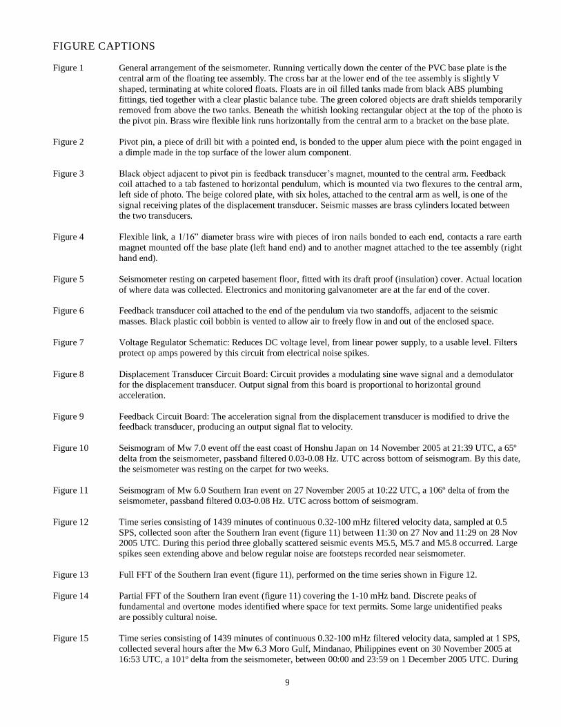
Figure 1 General arrangement of the seismometer. Running vertically down the center of the PVC base plate is thecentral arm of the floating tee assembly. The cross bar at the lower end of the tee assembly is slightly Vshaped, terminating at white colored floats. Floats are in oil filled tanks made from black ABS plumbingfittings, tied together with a clear plastic balance tube. The green colored objects are draft shields temporarilyremoved from above the two tanks. Beneath the whitish looking rectangular object at the top of the photo isthe pivot pin. Brass wire flexible link runs horizontally from the central arm to a bracket on the base plate.

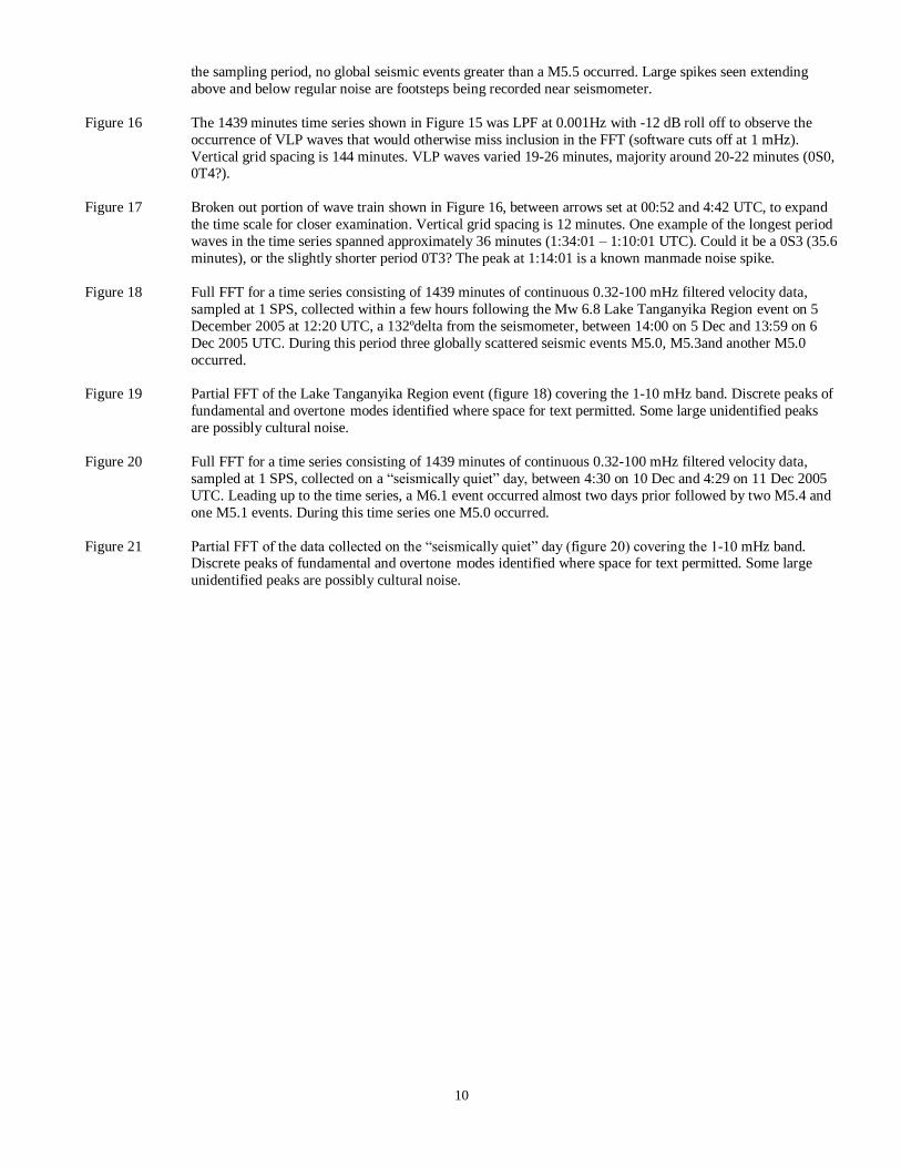
Figure 2 Pivot pin, a piece of drill bit with a pointed end, is bonded to the upper alum piece with the point engaged ina dimple made in the top surface of the lower alum component.

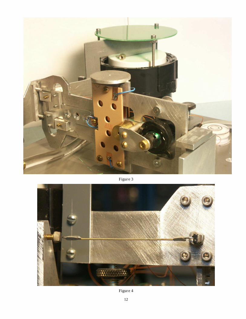
Figure 3 Black object adjacent to pivot pin is feedback transducer’s magnet, mounted to the central arm. Feedbackcoil attached to a tab fastened to horizontal pendulum, which is mounted via two flexures to the central arm,left side of photo. The beige colored plate, with six holes, attached to the central arm as well, is one of thesignal receiving plates of the displacement transducer. Seismic masses are brass cylinders located betweenthe two transducers.

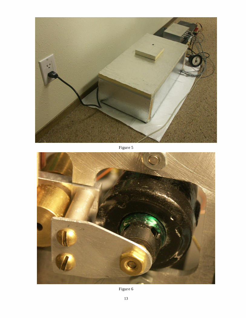
Figure 4 Flexible link, a 1/16” diameter brass wire with pieces of iron nails bonded to each end, contacts a rare earthmagnet mounted off the base plate (left hand end) and to another magnet attached to the tee assembly (righthand end).

Figure 5 Seismometer resting on carpeted basement floor, fitted with its draft proof (insulation) cover. Actual locationof where data was collected. Electronics and monitoring galvanometer are at the far end of the cover.

Figure 6 Feedback transducer coil attached to the end of the pendulum via two standoffs, adjacent to the seismicmasses. Black plastic coil bobbin is vented to allow air to freely flow in and out of the enclosed space.

Figure 7 Voltage Regulator Schematic: Reduces DC voltage level, from linear power supply, to a usable level. Filtersprotect op amps powered by this circuit from electrical noise spikes.

Figure 8 Displacement Transducer Circuit Board: Circuit provides a modulating sine wave signal and a demodulatorfor the displacement transducer. Output signal from this board is proportional to horizontal groundacceleration.

Figure 9 Feedback Circuit Board: The acceleration signal from the displacement transducer is modified to drive thefeedback transducer, producing an output signal flat to velocity.

Figure 10 Seismogram of Mw 7.0 event off the east coast of Honshu Japan on 14 November 2005 at 21:39 UTC, a 65ºdelta from the seismometer, passband filtered 0.03-0.08 Hz. UTC across bottom of seismogram. By this date,the seismometer was resting on the carpet for two weeks.

Figure 11 Seismogram of Mw 6.0 Southern Iran event on 27 November 2005 at 10:22 UTC, a 106º delta of from theseismometer, passband filtered 0.03-0.08 Hz. UTC across bottom of seismogram.

Figure 12 Time series consisting of 1439 minutes of continuous 0.32-100 mHz filtered velocity data, sampled at 0.5SPS, collected soon after the Southern Iran event (figure 11) between 11:30 on 27 Nov and 11:29 on 28 Nov2005 UTC. During this period three globally scattered seismic events M5.5, M5.7 and M5.8 occurred. Largespikes seen extending above and below regular noise are footsteps recorded near seismometer.

Figure 13 Full FFT of the Southern Iran event (figure 11), performed on the time series shown in Figure 12.

Figure 14 Partial FFT of the Southern Iran event (figure 11) covering the 1-10 mHz band. Discrete peaks offundamental and overtone modes identified where space for text permits. Some large unidentified peaksare possibly cultural noise.

Figure 15 Time series consisting of 1439 minutes of continuous 0.32-100 mHz filtered velocity data, sampled at 1 SPS,collected several hours after the Mw 6.3 Moro Gulf, Mindanao, Philippines event on 30 November 2005 at16:53 UTC, a 101º delta from the seismometer, between 00:00 and 23:59 on 1 December 2005 UTC. During

10

the sampling period, no global seismic events greater than a M5.5 occurred. Large spikes seen extendingabove and below regular noise are footsteps being recorded near seismometer.

Figure 16 The 1439 minutes time series shown in Figure 15 was LPF at 0.001Hz with -12 dB roll off to observe theoccurrence of VLP waves that would otherwise miss inclusion in the FFT (software cuts off at 1 mHz).Vertical grid spacing is 144 minutes. VLP waves varied 19-26 minutes, majority around 20-22 minutes (0S0,0T4?).

Figure 17 Broken out portion of wave train shown in Figure 16, between arrows set at 00:52 and 4:42 UTC, to expandthe time scale for closer examination. Vertical grid spacing is 12 minutes. One example of the longest periodwaves in the time series spanned approximately 36 minutes (1:34:01–1:10:01 UTC). Could it be a 0S3 (35.6minutes), or the slightly shorter period 0T3? The peak at 1:14:01 is a known manmade noise spike.

Figure 18 Full FFT for a time series consisting of 1439 minutes of continuous 0.32-100 mHz filtered velocity data,sampled at 1 SPS, collected within a few hours following the Mw 6.8 Lake Tanganyika Region event on 5December 2005 at 12:20 UTC, a 132ºdelta from the seismometer, between 14:00 on 5 Dec and 13:59 on 6Dec 2005 UTC. During this period three globally scattered seismic events M5.0, M5.3and another M5.0occurred.

Figure 19 Partial FFT of the Lake Tanganyika Region event (figure 18) covering the 1-10 mHz band. Discrete peaks offundamental and overtone modes identified where space for text permitted. Some large unidentified peaksare possibly cultural noise.

Figure 20 Full FFT for a time series consisting of 1439 minutes of continuous 0.32-100 mHz filtered velocity data,sampled at 1 SPS, collected on a“seismically quiet” day,between 4:30 on 10 Dec and 4:29 on 11 Dec 2005UTC. Leading up to the time series, a M6.1 event occurred almost two days prior followed by two M5.4 andone M5.1 events. During this time series one M5.0 occurred.

Figure 21 Partial FFT of the data collected on the “seismically quiet” day (figure 20) covering the 1-10 mHz band.Discrete peaks of fundamental and overtone modes identified where space for text permitted. Some largeunidentified peaks are possibly cultural noise.

11

FIGURES

Figure 1

Figure 2

12

Figure 3

Figure 4

13

Figure 5

Figure 6

14

Figure 7

15

Figure 8

16

Figure 9

17

Figure 10

Figure 11

18

Figure 12

Figure 13

19

Figure 14

Figure 15

20

Figure 16

Figure 17

21

Figure 18

Figure 19

22

Figure 20

Figure 21

23

APPENDIX A

TRANSFER FUNCTION FOR THE MK XXI BROADBAND SEISMOMETER.This Mathcad work sheet was originally created by Sean-Thomas Morrissey.

After downloading, the document was later reorganized for clarity by Allan Coleman.Last revised: 10/28/05

r = displacement transducer constant, volts/meter r 190288(measured at output of inverse filter)

M=sensor mass, kg M .07

C = feedback capacitor, farads C .000015

Rp = Proportional (DC) feedback resistor, ohms Rp 1000000

RI = Integrator feedback resistor, ohms RI 130000

RF = force transducer coil resistance RF 63

TI = Integrator time constant, seconds TI 100

To = Mechanical free period of sensor, seconds T0 3

Td = Displacement Transducer time constant (~= 0)

Generator Constant, Newton/Amps

............function requires m/s/s/amp:= G

m

sec2

ampGn 3.3 G

Gn

M G 47.1429

Damping:= S0 2

T0 S0 2.0944

1

2

1

Rp

S0 2

r G

TIRI

C

.5

0.6931

Effective "natural Period" (seconds):= Tn 2 C RI TI Tn 87.7399

Generalized Equation: Yi1

G C

s i 1 s i C RF

s i4 RF

r G

s i3 1

r G C

s i2 s iS0 2r G C

1

C Rp

1

C RI TI

24

Setting Constants: k1

G C n C RF a

RF

r G b

1

r G C c

S0 2r G C

1

C Rp d

1

C RI TI

i 1 2 600 fi 10 i 300( ) 0.01 i 2 fi s i j i s200 0.6283i

Evaluating: A i ks i 1 s i n

s i4 a s i3 b s i2 s i c d

veli Re Ai s i

maxv max vel( )

Ref. line, V/m/s: maxv 1.4148 103

Marking effective periods: FI1

TI Fn

1

Tn

1 103

0.01 0.1 1 10 100 1 1031

10

100

1 103

1 104VELOCITY RESPONSE OF BROADBAND SENSOR

F R E Q U E N C Y

Out

put:

Vol

ts/M

eter

/Sec

ond

FIFn