An Almost Ideal Demand System

Angus Deaton; John Muellbauer

The American Economic Review, Vol. 70, No. 3. (Jun., 1980), pp. 312-326.

Stable URL:

http://links.jstor.org/sici?sici=0002-8282%28198006%2970%3A3%3C312%3AAAIDS%3E2.0.CO%3B2-Q

The American Economic Review is currently published by American Economic Association.

Your use of the JSTOR archive indicates your acceptance of JSTOR's Terms and Conditions of Use, available athttp://www.jstor.org/about/terms.html. JSTOR's Terms and Conditions of Use provides, in part, that unless you have obtainedprior permission, you may not download an entire issue of a journal or multiple copies of articles, and you may use content inthe JSTOR archive only for your personal, non-commercial use.

Please contact the publisher regarding any further use of this work. Publisher contact information may be obtained athttp://www.jstor.org/journals/aea.html.

Each copy of any part of a JSTOR transmission must contain the same copyright notice that appears on the screen or printedpage of such transmission.

The JSTOR Archive is a trusted digital repository providing for long-term preservation and access to leading academicjournals and scholarly literature from around the world. The Archive is supported by libraries, scholarly societies, publishers,and foundations. It is an initiative of JSTOR, a not-for-profit organization with a mission to help the scholarly community takeadvantage of advances in technology. For more information regarding JSTOR, please contact support@jstor.org.

http://www.jstor.orgWed Feb 20 13:53:13 2008

An Almost Ideal Demand System

Ever since l c h a r d Stone (1954) first estimated a system of demand equations derived explicitly from consumer theory, there has been a continuing search for alternative specifications and functional forms. Many models have been proposed, but perhaps the most important in current use, apart from the original linear expendi- ture system, are the Rotterdam model (see Henri Theil, 1965, 1976; Anton Barten) and the translog model (see Laurits Christensen, Dale Jorgenson, and Lawrence Lau; Jorgen- son and Lau). Both of these models have been extensively estimated and have, in addition, been used to test the homogeneity and symmetry restrictions of demand the- ory. In this paper, we propose and estimate a new model which is of comparable gener- ality to the Rotterdam and translog models but which has considerable advantages over both. Our model, which we call the Almost Ideal Demand System (AIDS), gives an ar- bitrary first-order approximation to any de- mand system; it satisfies the axioms of choice exactly; it aggregates perfectly over consumers without invoking parallel linear Engel curves; it has a functional form which is consistent with known household-budget data; it is simple to estimate, largely avoid- ing the need for non-linear estimation; and it can be used to test the restrictions of homogeneity and symmetry through linear restrictions on fixed parameters. Although many of these desirable properties are possessed by one or other of the Rotterdam or translog models, neither possesses all of them simultaneously.

In Section I of the paper, we discuss the theoretical specification of the AIDS and justify the claims in the previous paragraph.

*University of Bristol, andBirkbeck College, London, respectively. We are grateful to David Mitchell for help with the calculations and to Anton Barten, David He ndry, Claus Leser, Louis Phlips, and a referee for helpful comments on an earlier version.

In Section 11, the model is estimated on postwar British data and we use our results to test the homogeneity and symmetry re- strictions. Our results are consistent with earlier findings in that both sets of restric- tions are decisively rejected. We also find that imposition of homogeneity generates positive serial correlation in the errors of those equations which reject the restrictions most strongly; this suggests that the now standard rejection of homogeneity in de-mand analysis may be due to insufficient attention to the dynamic aspects of con-sumer behavior. Finally, in Section 111, we offer a summary and conclusions. We be- lieve that the results of this paper suggest that the AIDS is to be recommended as a vehicle for testing, extending, and improving conventional demand analysis. This does not imply that the system, particularly in its simple static form, is to be regarded as a fully satisfactory explanation of consumers' behavior. Indeed, by proposing a demand system which is superior to its predecessors, we hope to be able to reveal more clearly the problems and potential solutions asso- ciated with the usual approach.

I. Specification of the AIDS

In much of the recent literature on sys- tems of demand equations, the starting point has been the specification of a func- tion which is general enough to act as a second-order approximation to any arbi-trary direct or indirect utility function or, more rarely, a cost function. For examples, see Christensen, Jorgenson, and Lau; W. Erwin Diewert (1971); or Ernst Berndt, Masako Darrough, and Diewert. Alterna- tively, it is possible to use a first-order approximation to the demand functions themselves as in the Rotterdam model, see Theil (1965, 1976); Barten. We shall follow these approaches in terms of generality but we start, not from some arbitrary preference

313 VOL. 70 NO. 3 DEATON AND MUELLBAUER: IDEAL DEMAND SYSTEM

ordering, but from a specific class of prefer- ences, which by the theorems of Muellbauer (1975, 1976) permit exact aggregation over consumers: the remesentation of market de- mands as if they were the outcome of deci- sions by a rational representative consumer. These preferences, known as the PIGLOG class, are represented via the cost or expendi- ture junction which defines the minimum expenditure necessary to attain a specific utility level at given prices. We denote this function c(u,p) for utility u and price vector p, and define the PIGLOG class by

With some exceptions (see the Appendix), u lies between 0 (subsistence) and 1 (bliss) so that the positive linearly homogeneous func- tions a(p) and b(p) can be regarded as the costs of subsistence and bliss, respectively. The Appendix further discusses this general model as well as the implications of the underlying aggregation theory.

Next we take specific functional forms for loga(p) and logb(p). For the resulting cost function to be a flexible functional form, it must possess enough parameters so that at any single point its derivatives ac/ap,, ac/au, a 2~/apiaP,, a *c/auap,, and a 2c/au2 can be set equal to those of an arbitrary cost function. We take

so that the AIDS cost function is written

mogeneous in p (as it must be to be a valid representation of preferences) provided that Xiai= l , C . y * . - X k y 6 = X j w . k ~ - It is alsoJ

straightforward to check that (4) has enough parameters for it to be' a flexible functional form provided it is borne in mind that, since utility is ordinal, we can always choose a normahation such that, at a point,

'1ogc/i3u2 =O. The choice of the functions a(p) and b(p) in (2) and (3) is governed partly by the need for a flexible functional form. However, the main justification is that this particular choice leads to a system of demand functions with the desirable proper- ties which we demonstrate below.

The demand functions can be derived di- rectly from equation (4). It is a fundamental property of the cost function (see Ronald Shephard, 1953, 1970, or Diewert's 1974 survey paper) that its price derivatives are the quantities demanded: dc(u,p)/ap, =qi. Multiplying both sides by p,/c(u,p) we find

where wi is the budget share of good i. Hence, logarithmic differentiation of (4) gives the budget shares as a function of prices and utility:

where

For a utility-maximizing consumer, total expenditure x is equal to c(u,p) and this equality can be inverted to give u as a function of p and x, the indirect utility function. If we do this for (4) and substitute the result into (6) we have the budget shares as a function of p and x; these are the AIDS demand functions in budget share form:

where q,P;, and y; are parameters. It can easily be checked that c(u,p) is linearly ho-

314 T H E AMERICAN ECONOMIC REVIEW JUNE 1980

where P is a price index defined by

( 9 ) log P =a , + 2 a, logp, k

+ -1 2 C Ykj logpk fog P,2 ; k

The restrictions on the parameters of (4) plus equation (7) imply restrictions on the parameters of the AIDS equation (8) . We take these in three sets

y. .=y.(12) U Jl

Provided ( l o ) , ( 1 l ) , and (12) hold, equation (8 ) represents a system of demand functions which add up to total expenditure (Xw,= 1 ) , are homogeneous of degree zero in prices and total expenditure taken together, and which satisfy Slutsky symmetry. Given these, the AIDS is simply interpreted: in the absence of changes in relative prices and "real" expenditure ( x / P ) the budget shares are constant and this is the natural starting point for predictions using the model. Changes in relative prices work through the terms yo; each y, represents l o 2 times the effect on the ith budget share of a 1 percent increase in the jth price with ( x / P ) held constant. Changes in real expenditure oper- ate through the Picoefficients; these add to zero and are positive for luxuries and nega- tive for necessities. Further interpretation is best done in terms of the claims made in the introduction.

A. Aggregation Over Households

The aggregation theory developed in Muellbauer (1975, 1976, of which the main relevant points are summarized in the Ap- pendix) implies that exact aggregation is possible if, for an individual household h, behavior is described by the generalization

The parameters kh can be interpreted as a sophisticated measure of household size which, in principle, could take account of age composition, other household character- istics, and economies of household size; and which is used to deflate the budget xh to bring it to a "needs corrected" per capita level. This allows a limited amount of taste variation across households. The share of aggregate expenditure on good i in the aggregate budget of all households, denoted Gi is given by

which, when applied to (8') gives

Define the aggregate index k by

where 2 is the average level of total expendi- ture xh. Hence (8")becomes

(8"') iF, =ai+'C yo logp, +pi log(Y/ k P ) J

This is identical in form to (8') and this confirms that under these assumptions ag- gregate budget shares correspond to the de- cisions of a rational representative house-hold whose preferences are given by the AIDS cost function ( 4 ) and whose budget is given by Y / k , the "representative budget level."

The index k has an interesting interpreta- tion. If each household had the same tastes (kh= 1 , all h), k would be an index of the

VOL. 70 NO. 3 DEATON AND MUELLBAUER: IDEAL DEMAND SYSTEM 315

equality of the distribution of household budgets. In fact, this index is identical to Theil's (1972)entropy measure of equality Z deflated by the number of households H, where logZ = -C ( x h / X ) l o g ( x h / X )and X is the aggregate budget; Z reaches its maxi- mum level of H when there is perfect equal- ity so that xh=2,all h. Therefore as inequal- ity increases, k =Z / H decreases and the representative budget level increases. When k,, differs across households, for example, because of differences in household com-position, the index k reflects not only the distribution of budgets but the demographic structure. Ideally, one might attempt to model the variation of kh with household characteristics in a cross-section study and, given time-series data on the joint distribu- tion of household budgets and characteris- tics, construct a series for k for use in fitting (8"'). Data limitations have prevented us from carrying out this proposal in the em- pirical application below. To the extent that k is constant or uncorrelated with 2 orp , no omitted variable bias arises from our proce- dure of omitting k and redefining a: =~ u ,-Pi log k* where k* is the constant or sample mean value of k .

When the distribution of household bud- gets and household characteristics is invar- iant except for equiproportional changes in household budgets, k is constant. In this case there is considerable extra scope for taste variations in the individual demand functions without altering the validity of the representative consumer hypothesis em- bodied in (8"'). Indeed, it turns out that not only aih,all i , but also yQh,all i j , can differ over households. The ai and y, parameters in (8"') are then weighted averages of the micro parameters.

B. Generality of the Model

The flexible functional form property of the AIDS cost function implies that the demand functions derived from it are first- order approximations to any set of demand functions derived from utility-maximizing behavior. The AIDS is thus as general as

other flexible forms such as the translog or the Rotterdam models. However, if maxi-mizing behavior is not assumed but it is simply held that demands are continuous functions of the budget and of prices, then the AIDS demand functions (8 ) (without the restrictions (1 1 ) and (12)) can still pro- vide a first-order approximation. In general, without maximizing assumptions, we can think of the budget shares w, as being un- known functions of logp and logx . From ( 8 ) and (9) , the AIDS has derivatives aw, /arogx=p , and aw, /a logpJ= ~ , - p , ~ -P,CyJ,logp, so that, at any point, P and y can be chosen so that the derivatives of the AIDS will be identical to those of any true model. Given that the a varameters act as intercepts, the AIDS can thus provide a local first-order approximation to any true demand system, whether derived from the theory of choice or not. This property is important since it means that tests of homo- geneity of symmetry are set within a main- tained hypothesis which makes sense and would be widely accepted in its own right.

Generality is not without its problems, however. There is a large number of param- eters in (18) and on most data sets these are unlikely to be all well determined. It is thus important that there should exist some straightforward procedure for eliminating unnecessary parameters without untoward consequences for the properties of the model. In the AIDS. this can be done bv placing whatever restrictions on y, parame-ters are thought to be empirically or theor- etically plausible. As we shall see below, in many cases it will be possible to impose these restrictions on a single equation basis. One obvious restriction is that for some pairs ( i , j ) , y,, should be zero; for such pairs the budget share of each is independent of the price of the other if ( x / P ) is held con- stant. It can be shown that y,. has approxi- mately the same sign as the compensated cross-price elasticity and this is also useful in suggesting prior restrictions. We should not however expect all the y,s to be zero; the resulting model, w,= a, + log(x / P ) is extremely restrictive and has been tested and rejected by Deaton (1978).

316 THE AMERICAN ECONOMIC REVIEW JUNE 1980

C . Restrictions

If we start from equations (8) and (9) as our maintained hypothesis, we can examine the effects of the restrictions (10)-(12) which are required to make the model con- sistent with the theory of demand. The con- ditions (10) are the adding-up restrictions; as can easily be checked from (8), these ensure that 2 wi=1. Homogeneity of the demand functions requires restriction (1 1) which can be tested equation by equation. Slutsky sym-metry is satisfied by (8) if and only if the symmetry restriction (12) holds. As is true of other flexible functional forms, negatioity cannot be ensured by any restrictions on the parameters alone. It can however be checked for any given estimates by calculat- ing the eigenvalues of the Slutsky matrix so, say. In practice, it is easier to use not sG but k . . = p g . s . . / x ,J V , the eigenvalues of which have r/

the same signs as those of so and which are given by

where So is the Kronecker delta. Note that apart from this negativity condition, all the restrictions are expressible as linear con-straints involving only the parameters and so can be imposed globally by standard techniques.

D. Estimation

In general, estimation can be carried out by substituting (9) in (8) to give

and estimating this non-linear system of equations by maximum ldcelihood or other methods with and without the restrictions (11) and (12). (Note that since the data add up by construction, (10) is not testable.) Equation (15) is not particularly difficult to estimate since the first-order conditions for

likelihood maximization are linear in a and y given p and vice versa so that "concentra- tion" allows iteration on a subset of the parameters (see for example, Deaton, 1975, pp. 46-49). Although all the parameters in (15) are identified given sufficient variation in the independent variables, in many exam- ples the practical identification of a, is likely to be problematical. This parameter is only identified from the a,s in (15) by the presence of these latter inside the term in braces, originally in the formula for log P , equation (9). However, in situations where individual prices are closely collinear, log P is unlikely to be very sensitive to its weights so that changes in the intercept term in (15) due to variations in a, can be offset in the a s with minimal effect on log P . This can be overcome in practice by assigning a value to a, a priori. Since the parameter can be inter- preted as the outlay required for a minimal standard of living when prices are unity (usually in the base year; see the Appendix), choosing a plausible value is not difficult.

However, in many situations, it is possible to exploit the collinearity of the prices to yield a much simpler estimation technique. Note from (8) that if P were known, the model would be linear in the parameters a , p, and y, and estimation (at least without cross-equation restrictions such as symme-try) can be done equation by equation by OLS which, in this case and given normally distributed errors, is equivalent to maximum ldcelihood estimation for the system as a whole. The adding-up constraints (10) will be automatically satisfied by these esti-mates. In situations where prices are closely collinear, it may well be adequate to ap-proximate P as proportional to some known index P*, say. One obvious candidate in view of (8) and (9) is Stone's (1953) index logP* =Zw, logp,. If P=@P* say, then ( 8 ) can be estimated as

Note that in this framework the a, parame-ters are identified only up to a scalar multi- ple of pi;if we write a: =a, -Pilog+, it is

VOL. 70 NO. 3 DEATON AND MUELLBAUER: IDEAL DEMAND SYSTEM 31 7

easily seen that Ca,* = O is still required for adding up, since C P, = 0 .

In the empirical results below we shall estimate both (15) and (16), and show that the latter is an excellent approximation to the former. However, it must be emphasized that (16) exists only as an approxima-tion to (15) and will only be accurate in specific circumstances, albeit widely occur- ring ones in time-series estimation. Note finally that if single equation estimation is used to investigate likely restrictions amongst the y parameters, as is suggested in Part B above. the constrained OLS estimates will no longer automatically be maximum likelihood, efficient, or satisfy adding up. Hence. once the restrictions have been selected, (15) should be used to reestimate the whole system.

E. Relationship with Budget Studies and with the Rotterdam Model

The Engel curves corresponding to (8 ) take the form p,q, = t , x + Pix logx for ap- propriate functions of prices t,. These are clearly not linear except in the proportional case when P , = O The model thus allows a possible reconciliation between time-series models, which have to date required linear- ity of Engel curves for aggregation with cross-section results, which typically find evidence of nonlinearity. Indeed, the PIG-LOG Engel curve w,= (, + Pi log x was used as early as 1943 by Holbrook Working and has recently been recommended by Claus Leser (1963, 1976) as providing an excellent fit to cross-section data in a wide range of circumstances.

In the time-series context, the AIDS has a close relationship to the Rotterdam model of Theil (1965, 1976) and Barten. The first difference form of (8 ) is

which no longer involves the a parameters except through Alog P . This dependence can

be seen by writing (17) in full, i.e.,

Again, all the parameters (except a,) are theoretically identified, but in practice the substitutability between yUs and P,a,s in fit- ting (18) if prices are nearly collinear means that, in such cases, the only practical way of estimating (17) is to replace AlogP by some index, for example, A(Zwklogpk) as before or by its approximation ZwkAlogpk. In the latter case, the right-hand side of (17) be-comes identical to the right-hand side of the Rotterdam model which is

The dependent variable is different in the AIDS; instead of w,Alogq, we have Aw, or w,Alogw,. Thus, by replacing the dependent variable w,A log q, in the Rotterdam model by w,A log w,, an addition of w,A log(p , /x ) , we generate the first-difference form of the AIDS. The similarity between the two mod- els is quite striking in this form; both are effectively linear and both can be used to test homogeneity and symmetry with only linear restrictions on constant parameters. Note however that the parameters have quite different interpretations in the two models so that, for example, the negativity condition applies directly to the matrix of price effects in the Rotterdam model which is not the case for the AIDS. The crucial difference between the two models is that (17), unlike (19), is derived from explicit demand functions, (8) ,and an explicit char- acterization of preferences, (4) . For the pre- diction of demand this difference may not be vitally important, but in many other con- texts, for example in calculating cost-of-living indices, household equivalence scales, or optimal tax rates, the ability to link

318 THE AMERICAN ECONOMIC REVIEW JUNE 1980

estimated parameter values to preferences themselves becomes of great significance.

11. An Application to Postwar British Data

In this section we estimate the model using annual British data from 1954 to 1974 inclusive on eight nondurable groups of consumers' expenditure, namely, food, clothing, housing services, fuel, drink and tobacco, transport and communication services, other goods, and other services. As discussed in Section I, Part A above, if we assume that the index k in (8"') is either constant or that its deviations are indepen- dently distributed from those of the average budget i?and of prices, no biases result from its omission. In particular, we allow the in- tercepts in (8"') to absorb the -Pilog k terms. We then proceed by first following the strategy outlined in Section I, Part D, setting IogP* =E w, logp, for each year and estimating equation (16) for each good sep- arately by OLS. The system is then reesti- mated, equation by equation, and again using P*, in order to test the homogeneity condition. Equation (1 1) is imposed by sub- stitution so that instead of (16), we estimate

At this stage, F-ratios are calculated equa- tion by equation to test the validity of the restriction.

The next stage is to impose symmetry of y, at this point replacing P* by the "correct" price index (9) with a, set to some ap-propriate value. Since symmetry, unlike homogeneity or the unrestricted model, involves cross-equation restrictions, the vari- ance-covariance matrix of the residuals for the first time plays a part in the estimation. Since this is unknown a priori, normal prac- tice would be to replace it by its maximum likelihood estimate. However, with only twenty-one observations, this is not practi- cable for equation (15) since, with so many parameters in each equation, the likelihood can be made arbitrarily large by malung any

one equation fit perfectly.' This difficulty can only be resolved by assuming a particu- lar structure for the variance-covariance matrix of the residuals. Following Deaton (1975, p. 39), we assume v = a 2 ( I - ii'), where V is the variance-covariance matrix of the residuals, a2 is a (positive) parameter to be estimated, I is an n x n identity matrix and i is a vector each of the elements of which is (n)-'/2. In this case, maximum-like- lihood estimation reduces to least squares so that instead of minimizing the determinant of the matrix of residual cross products, we minimize its trace. The likelihood values quoted below are calculated on this assump- tion. Once again, maximum use is made of substitution in the estimation so that, under symmetry, (15) is estimated using only the fourteen independent cu*s and pis and the twenty-eight parameters forming the upper right-hand triangle of y with its final row and column deleted. We now check that P* and P are sufficiently close to allow com- parison of likelihoods both by direct evalua- tion of both indices and by reestimation of the unrestricted and homogeneous models using P as evaluated from the symmetric estimates. It is also possible to check con- cavity at this stage by using the symmetric parameter estimates to calculate the eigen- values of the matrix in (14). Finally, the whole process is repeated with the model written in first differences, that is, equation (17) with the addition of intercepts. Collin- earity prevented any successful attempt to link P to the parameter estimates in these regressions; instead, the value of P calcu-lated from the symmetric estimation in levels was used throughout.

Note that we choose to test symmetry whether or not homogeneity is rejected. This procedure has been criticized by Grayham Muon who suggests that optimal inference requires that further testing be abandoned as soon as a rejection is encountered. Muon's criticism would be correct if we were certain of our maintained hypothesis, but to some extent this is a matter of choice. Many economists would choose not to test

'We are grateful to Teun Kloek for pointing this out to us.

VOL. 70 NO. 3 DEATONAND MUELLBAUER: IDEAL DEMAND SYSTEM

TABLE1-THE PARAMETER AND TESTS OF HOMOGENEITY UNCONSTRAINED ESTIMATES (I-Values in Parentheses)

S.E.E. Commodity i a: p, y , , ~2 b) b4 Y,5 b6 Yi7 718 ~ Y I ,(lo-') R 2 D'W'

I -

Food 1.221 -0160 0.186 -0.077 -0.013 -0.020 -0.058 0.032 0.015 -0.098 -0.033 (7.4) (-6.1) (9.8) (-4.3) (-0.8) (-1.1) (-6.2) (1.3) (0.7) (-4.2) (-4.4)

Clothing -0.482 0.091 0.033 0.016 -0.024 -0.026 -0.029 0.014 0.033 -0.049 -0.032 (-3.1) (3.7) (1.8) (1.0) ( - 6 ) ( -1 .5 (-3.3) (0.6) (1.6) (-2.2) (-4.5)

Housing 0.793 -0.104 -0.082 -0.9 0.088 0.9 0.033 -0.055 -0.030 0.098 0.051 (6.3) (-5.1) (-5.6) (-0.7) (7.2) (0.7) (4.7) (-2.9) ( - 1.8) (5.5) (9.1)

Fuel -0.159 0.033 -0.042 0.010 -0.011 0.037 -0.004 0.022 0.007 -0.031 -0.010 (-0.8) 1.0) 8 (0.4) (-0.5) 6 (-03) (0.7) (0.3) (-1.1) (-1.1)

Drink and -0.043 0.028 -0.043 0.034 -0.027 -0.020 0.056 0.005 -0.018 0.014 0.001 Tobacco (-0.3) (1.2) (-2.6) (2.2) (- 1.9) (- 2 (6.9) (0.2) (-0.9) (0.7) (0.0)

Transport and -0.061 0.029 -0.022 -0.012 -0.002 0.011 0.060 -0.023 -0.024 0.053 0 . W Communicat~orI(-0.9) (2.6) (-2.7) ( - 1.6) (-0.3) (1.4) (15.2) (-2.2) (-2.6) (5.3) (13.1)

Other Goods -0.038 0.022 0.001 -0.003 -0.001 -0.006 -0.030 0.007 0.032 -0.006 -0.005 (-0.2) (0.9) (0.0) (-0.2) (-0.0) (-0.3) (-3.4) (0.3) ( I . ) (-0.2) (0.7)

Other Services -0.231 0.060 -0.032 0.041 -0.01 1 0.014 -0.028 -0.003 -0.015 0.019 -0.014 - 5 ) 2 4 8 (2.4) (-0.7) (0.8) (-3.1) (-0.1) (-0.7) (0.9) (-2.0)

homogeneity, treating absence of money illusion as a maintained hypothesis; the test of symmetry would then be the interesting one. Even if the maintained hypothesis turns out to be false, tests based on it are not necessarily without interest. Few if any tests in econometrics are carried out within the framework of maintained hypotheses which are even widely accepted, let alone of unchallengeable validity.

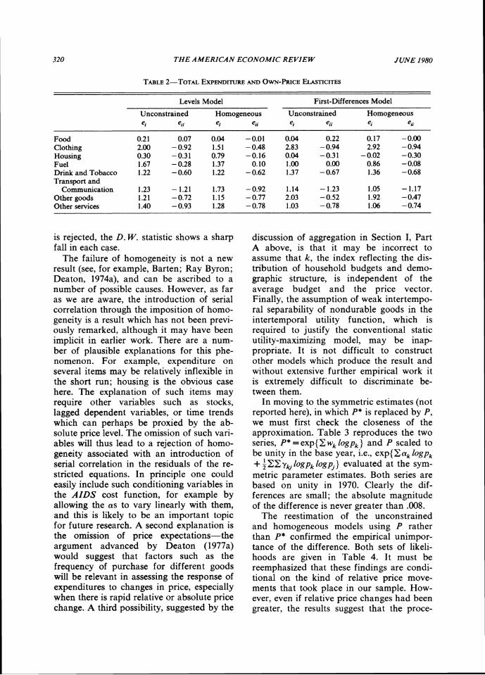
Table 1 reports the first-stage estimates of (16) using P* and without any constraints on the parameters save (10) which are auto- matically and costlessly satisfied. The esti- mates of /? classify food and housing as necessities while the other goods are luxuries. A large number of y coefficients are significantly different from zero; twenty- two out of sixty-four have t-values ab-solutely larger than 2. Even so, none of the variables considered have any detectable effect on the value share for fuel and very few have influence in the other goods or other services equations. Similarly, the prices of fuel, of transport and communica- tion, and of other services have little or no effect anywhere (except, of course, through P* and the value share itself), while the prices of food, drink and tobacco, and of other services appear with considerable reg- ularity. The total expenditure and own-price elasticities are shown in the first two col-

umns of Table 2 and, although food has an (insignificant) positive price elasticity, these numbers appear both credible and in line with other studies. Note the general price inelasticity of demand; only transport and communication appear to be price elastic.

Table 1 also shows, in the column headed 2 y V , the row sums of the unconstrained yi matrix; this number shows lo2 times the absolute effect on each value share of a 1 percent increase in all prices and total ex- penditure. Under homogeneity, this should be zero and the bracketed numbers given are t-tests of the significance of the devia- tion from zero. These numbers are, of course, identical to the square roots of the F-ratios obtained by comparing the residual sums of squares of equations (16) and (20). Hence, a proportional increase in prices and expenditure will decrease expenditure on food and on clothing, and increase expendi- ture on housing and transport and com-munication. These are also the commodities for which the elasticities suffer the largest changes between columns 1 and 2 and col- umns 3 and 4 of Table 2. Other deviations from homogeneity appear not to be signifi- cant. The final columns of Table 1 give equations standard errors, the R~ and Durbin-Watson (D. W.) statistics for free and restricted estimation. Note that for the four commodity groups where homogeneity

320 THE AMERICAN ECONOMIC REVIEW JUNE 1980

TABLE2-TOTAL EXPENDITURE AND OW-PRICE ELASTICITES

Levels Model First-Differences Model

Unconstrained Homogeneous Unconstrained Homogeneous ei eii ei

Food Clotlung Housing Fuel Drink and Tobacco Transport and

Communication Other goods Other services

is rejected, the D.W. statistic shows a sharp fall in each case.

The failure of homogeneity is not a new result (see, for example, Barten; Ray Byron; Deaton, 1974a), and can be ascribed to a number of possible causes. However, as far as we are aware, the introduction of serial correlation through the imposition of homo- geneity is a result which has not been previ- ously remarked, although it may have been implicit in earlier work. There are a num- ber of plausible explanations for this phe- nomenon. For example, expenditure on several items may be relatively inflexible in the short run; housing is the obvious case here. The explanation of such items may require other variables such as stocks, lagged dependent variables, or time trends which can perhaps be proxied by the ab- solute price level. The omission of such vari- ables will thus lead to a rejection of homo- geneity associated with an introduction of serial correlation in the residuals of the re- stricted equations. In principle one could easily include such conditioning variables in the AIDS cost function, for example by allowing the as to vary linearly with them, and this is likely to be an important topic for future research. A second explanation is the omission of price expectations-the argument advanced by Deaton (1977a) would suggest that factors such as the frequency of purchase for different goods will be relevant in assessing the response of expenditures to changes in price, especially when there is rapid relative or absolute price change. A third possibility, suggested by the

eii el eii ei ei i

discussion of aggregation in Section I, Part A above, is that it may be incorrect to assume that k, the index reflecting the dis- tribution of household budgets and demo- graphic structure, is independent of the average budget and the price vector. Finally, the assumption of weak intertempo- ral separability of nondurable goods in the intertemporal utility function, which is required to justify the conventional static utility-maximizing model, may be inap-propriate. It is not difficult to construct other models which produce the result and without extensive further empirical work it is extremely difficult to discriminate be- tween them.

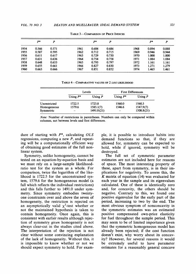
In moving to the symmetric estimates (not reported here), in which P* is replaced by P, we must first check the closeness of the approximation. Table 3 reproduces the two series, P*=exp{2w, logp,) and P scaled to be unity in the base year, i.e., exp{2ak logp, + i2Eyk, logp, logp,) evaluated at the sym- metric parameter estimates. Both series are based on unity in 1970. Clearly the dif-ferences are small; the absolute magnitude of the difference is never greater than .008.

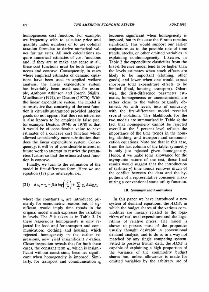
The reestimation of the unconstrained and homogeneous models using P rather than P* confirmed the empirical unimpor- tance of the difference. Both sets of likeli- hoods are given in Table 4. It must be reemphasized that these findings are condi- tional on the kind of relative price move-ments that took place in our sample. How- ever, even if relative price changes had been greater, the results suggest that the proce-

321 VOL. 70 NO. 3 DEATON AND MUELLBAUER: IDEAL DEMAND SYSTEM

TABLE4-COMPARATIVEVALUES OF 2 LOG LIKELIHOOD

Levels First Differences Using P* Using P Using P* Using P

Unrestricted 1722.5 1723.8 1560.0 1560.3 Homogeneous Symmetric

1579.6 -

1585.1(7) 1491.0(21)

1546.6 -

1547.9(7) 1508.8(21)

Note: Number of restrictions in parentheses. Numbers can only be compared within columns, not between levels and first differences.

dure of starting with P*, calculating OLS regressions, computing a new P, and repeat- ing will be a computationally efficient way of obtaining good estimates of the full non- linear system.

Symmetry, unlike homogeneity, cannot be tested on an equation-by-equation basis and we must rely on a large-sample likelihood- ratio test for the system as a whole. For comparison, twice the logarithm of the like- lihood is 1722.5 for the unconstrained sys- tem, 1579.6 for the homogeneous model (a fall which reflects the individual restrictions) and this falls further to 1491.0 under sym- metry. Since symmetry embodies twenty-one constraints over and above the seven of homogeneity, the restriction is rejected on an asymptotically valid X2-test whether or not the maintained hypothesis is taken to contain homogeneity. Once again, this is consistent with earlier results although rejec- tion of symmetry given homogeneity is not always clear-cut in the studies cited above. The interpretation of the rejection is not clear without some convincing explanation of the lack of homogeneity. Without this, it is impossible to know whether or not we should expect symmetry to hold. For exam-

ple, it is possible to introduce habits into demand functions so that, if they are allowed for, symmetry can be expected to hold, while if ignored, symmetry will be destroyed.

The full set of symmetric parameter estimates are not included here for reasons of space. The most interesting property of these, apart from symmetry, is in their im- plications for negativity. To assess this, the K matrix of equation (14) was evaluated for each year in the sample and its eigenvalues calculated. One of these is identically zero and, for concavity, the others should be negative. Contrary to this, we found one positive eigenvalue for the early part of the period, increasing to two by the end. The most obvious symptom of nonconcavity in the symmetric estimates was an estimated positive compensated own-price elasticity for fuel throughout the sample period. This may seem to be of limited importance given that the symmetric homogeneous model has already been rejected; if the cost function doesn't exist, why worry about its concav- ity? However, for several reasons it would be extremely useful to have parameter estimates for a reasonably general concave

322 THE AMERICAN ECONOMIC REVIEW JUNE 1980

homogeneous cost function. For example, we frequently wish to calculate price and quantity index numbers or to use optimal taxation formulae to derive numerical val- ues for tax rates. All such calculations re- quire numerical estimates of cost functions and, if they are to make any. sense at all, these cost functions must be both homoge- neous and concave. Consequently, in cases where empirical estimates of demand equa- tions have been used in applied welfare analysis, the linear expenditure system has invariably been used; see, for exam-ple, Anthocy Atkinson and Joseph Stiglitz, Muellbauer (1974), or Deaton (1977b). With the linear expenditure system, the model is so restrictivethat concavitv of the cost func- tion is virtually guaranteed provided inferior goods do not appear. But this restrictiveness is also known to be empirically false (see, for example, Deaton, 1974b or 1978) so that it would be of considerable value to have estimates of a concave cost function which allowed considerably more substitution than does the linear expenditure system. Conse- quently, it will be of considerable interest in future work to attempt to restrict the param- eters further so that the estimated cost func- tion is concave.

Finally, we turn to the estimation of the model in first-difference form. Here we use equation (17) plus intercepts, i.e.,

where the constants qi are introduced pri- marily for econometric reasons but, if sig- nificant, would imply time trends in the original model which expresses the variables in levels. The P is taken as in Table 3. In these regressions homogeneity is only re-jected for food and for transport and com- munication; clothing and housing, which rejected homogeneity in the earlier re-gressions, now yield insignificant F-ratios. Closer inspection reveals that for both these cases, the constant term q,,which is insigni- ficant without constraints, becomes signifi- cant when homogeneity is imposed. Simi- larly, for transport and communication qj

becomes significant when homogeneity is imposed, but in this case the F-ratio remains significant. This would support our earlier conjectures as to the possible role of time trends, stocks, or other omitted variables in explaining nonhomogeneity. Likewise, in Table 2 the expenditure elasticities from the first-difference model tend to be higher than the levels estimates when stock effects are likely to be important (clothing, other goods) and lower when one would expect short-run total expenditure effects to be limited (food, housing, transport). Other-wise, the first-difference parameter esti-mates, homogeneous or unconstrained, are rather close to the values originally ob-tained. As with levels, tests of concavity with the first-difference model revealed several violations. The likelihoods for the two models are summarized in Table 4; the fact that homogeneity cannot be rejected overall at the 5 percent level reflects the importance of the time trends in the hous- ing, clothing, and transport and communi- cation equations. Note too that in this case, from the last column of the table, symmetry is only just rejected given homogeneity. Hence, if we make some allowance for the asymptotic nature of the test, these final results would suggest that the introduction of (arbitrary) time trends removes much of the conflict between the data and the hy- pothesis of a representative consumer maxi- mizing a conventional static utility function.

III. Summary and Conclusions

In this paper we have introduced a new system of demand equations, the AIDS, in which the budget shares of the various com- modities are linearly related to the loga- rithm of real total expenditure and the loga- rithms of relative vrices. The model is shown to possess most of the properties usually thought desirable in conventional demand analysis, and to do so in a way not matched by any single competing system. Fitted to postwar British data, the AIDS is capable of explaining a high proportion of the variance of the commodity budget shares but, unless allowance is made for omitted variables by the arbitrary use of

323 VOL. 70 NO. 3 DEATON AND MUELLBAUER: IDEAL DEMAND SYSTEM

time trends, does so in a way which is inconsistent with the hypothesis of con-sumers making decisions according to the model's demand functions governed by the conventional static budget constraint. These results suggest that influences other than current prices and current total expenditure must be systematically modelled if even the broad pattern of demand is to be explained in a theoretically coherent and empirically robust way. Whether these developments generalize the static framework by including stock effects, errors in price perceptions, or by going beyond the assumption of weak intertemporal separability on which the static model rests. we believe that the AIDS. with its simplicity of structure, generality, and conformity with the theory, offers a platform on which such developments can proceed.

APPENDIX:AIDS I N T H E CONTEXT OF AGGREGATIONTHEORY

In Muellbauer (1975, 1976), a definition of the existence conditions for a representa- tive consumer is given which allows more general behavior than the parallel linear En- gel curves which are required if average demands are to be a function of the average budget. We know that in general, the average budget share

is a function of prices and the complete distribution vector ( x , , x , ,. . . ,x,). A repre-sentative consumer exists in Muellbauer's sense if each can be written as a function of prices and the same single scalar x,, itself a function of prices and the distribution vector. This scalar, which can be thought of as marking a position in the distribution of xs, is the representative budget level. Muellbauer shows that for an x, to exist such that

C xhwih(xh,p) /Cxh= . , x H , p ) , p }w i { x o ( x I t . . h

the individual budget share equations must

have the "generalized linear" ( G L ) form:

(A21

wih(xh,p)= + B , ( P )+ C , ~ ( P >v h ( x h > ~ ) A i ( ~ )

where vh, A,, B,, and C,, are functions satis- fying C , A i = C i C j h = C h C j h = Oand C B , = 1 . Clearly, ( A l ) goes beyond the usual for-mulation of x,= .?, and, as we shall see below, allows us to incorporate into the demand functions features of the expendi- ture distribution other than the mean.

Of particular interest is the case where x , is independent of prices, depending only on the individual xs. This occurs if, and only if, the uh function in ( A 2 ) restricts to

where a is a constant and kh,although not a function of xh, and p is free to vary from household to household. In this case, the budget shares are said to have the "price-in- dependent generalized linear" form (PIGL). Note the special case of (A3) as a+0, i.e.,

For obvious reasons, this is referred to as the PIGLOG case. By substituting (A3) in (A2) , ( A l ) can be used to give an explicit form for x,, viz.,

If we assume that individual behavior is preference consistent, the cost function cor- responding to PIGL takes the form

which as a tends to zero takes the PIGLOG form

where a ( p ) and b ( p ) are linear homoge-neous concave functions, a is the constant

324 THE AMERICAN ECONOMIC REVIEW JUNE 1980

parameter of (A3), and (with some excep- tions discussed below) 0 <u < 1 . The quan- tity kh can be used to allow for family composition effects within PIGL; for the standard or "reference" household kh is unity.

Since the AIDS is a member of the PIG-LOG family, and hence of PIGL, we can achieve maximum generality by discussing some of the important properties of this class. If, omitting the household subscript, we write q, for the quantity demanded of good i , then, by the derivative property of the cost function, q,=ac/ap, so that w,= p,q,/x =a logc/a logp,. Hence from (A6), taking kh= 1 , and differentiating

where a,=a log a / a logp, and b,= a log b / a logp,. Hence, substituting x for c,

where, from (A6), u =( x a-a a ) / ( b a-a a ) or from (A7), u = (log x - log a)/(log b -log a). Similarly, when a =0,

Equations (A9) and (A10) have attractive interpretations. Cost c(u,p) is increasing in utility as long as b(p ) is greater than a(p)-note that this does not depend on the sign of a-SO that as u increases from 0 to 1 , c(u,p) increases from a(p ) to b ( p ) with w, moving from a, to b,. Hence a total expendi- ture of a ( p ) can be thought of as "poverty" expenditure with associated expenditure pattern a,, while b(p ) is "affluence" ex-penditure with budget shares b,. On this interpretation x =a ( p ) and x = b(p ) are the equations of the tangents to the poverty and affluence indifference curves, respec-tively, u =0 and u = 1 . From (A6 ) therefore, we see that the tangent to the indifference curve actually attained is the mean of order a of poverty and affluence tangents, the weights depending on the welfare level or

outlay of the household. This averaging is even more obvious in the value share equa- tions (A9) and (A10). Since ( 1 -u)(a/x)* and u(b/x)" sum to unity, as do ( 1 - u) and u, these equations give the actual budget shares as weighted averages of a, and b,.

Since the value shares of luxuries increase with total outlay and hence with u, we can characterize luxuries and necessities simply by whether b, is greater than or less than a,. Inferior goods are not excluded under PIGL and it is straightforward to construct exam- ples from both (A9) and (A10).

Note finally that there are restrictions on the possible set of x and p over which the cost function and the associated demands are valid. One set of restrictions is implied by the necessity that, for all i , 0 <w, < 1 . The upper bound is relevant when b,>a, and implies that u = ( x a - a a ) / ( b a- a a )< min,[{l - a,(a/x>.}/{(b/x)ab,- (a/x>.a,}]. The lower bound, relevant when b, <a, re-quires similarly that u =( x a- a a ) / ( b a-a a ) > r n a ~ , [ ( a / x ) ~ a , / -{ ( a / ~ ) ~ a ,( b / ~ ) ~ b , ) ] . The second set of restrictions are those re- quired to ensure that the cost function is concave. From (A6), we can see that a sufficient condition for concavity of c(u,p) is that a ( p ) and b(p ) be concave and that 0 <u < 1 . However, this is by no means nec- essary. If b(p ) is "more concave" than a(p) , then c(u,p) is concave for u > O and for a range of u> 1. It can be shown that the PIGL cost function is concave for all x >0, p >0 if and only if a,=b, for all i , and a ( p ) and b ( p ) are concave. In this not very inter- esting case, preferences are homothetic.

The practical application of the PIGL class requires selection of specific functional forms for the functions a ( p ) and b(p ) ;those leading to the AIDS have been discussed in the text. However, the PIGL class is related to two other well-known models. Note first that if a = 1, and kh= 1 , (A6) becomes the Gorman polar form. The PIGL class thus includes all models with linear Engel curves, for example, linear expenditure system, the quadratic utility function, as special cases. Perhaps less obviously, a weakly restricted form of the indirect translog is also PIG-LOG. From Jorgenson and Lau the translog

325 VOL. 70 NO. 3 DEATONAND MUELLBAUER: IDEAL DEMAND SYSTEM

indirect utility function is

(A l l ) u=a,+ 2 ailog i

where we can choose Xa, = - 1 and ,E,, =4, as arbitrary normalizations. Write XkPki= pMi,then if we impose the additional restric-tion that XiPMi=O, (A1 1) solves explicity for logc(u,p) to

u - XX PClogpilogp, -X ailogpi-a,--

This is of the general form logc(u,p)= loga(p) +u/log h(p) for appropriate choice of a(p) and h(p). Using log h(p) = 1/log{ b(p)/a(p)) to define b(p) and sub-stituting, we see that (A12) is identical to (A7). Hence, in this case (ZipMi=0) and in this case only, the indirect translog allows consistent aggregation. No such result holds for any interesting subcase of the direct translog.

REFERENCES

A. B. Atkinson and J. E. Stiglitz, "The Structure of Indirect Taxation and Economic Effi-ciency," J. Publ. Econ., Apr. 1972, 1, 97- 119.

A. P. Barten, "Maximum Likelihood Estima-tion of a Complete System of Demand Equations," Euro. Econ. Rev., Fall 1969, 1, 7-73.

E. R. Berndt, M. N. Darrough, and W. E. Diewert, "Flexible Functional Forms and Expenditure Distributions: An Applica-tion to Canadian Consumer Demand Functions," Int. Econ. Reu., Oct. 1977, 18, 651-75.

R. P. Byron, "A Simple Method for Estimat-ing Demand Systems under Separable Utility Assumptions," Reo. Econ. Stud., Apr. 1970, 37, 261-74.

L. R. Christensen, D. W. Jorgenson, and L. J. Lau, "Transcendental Logarithmic Utility Functions," Amer. Econ. Rev., June 1975, 65, 367-83.

A. S. Deaton, (1974a) "The Analysis of Con-sumer Demand in the United Kingdom, 1900- 1970," Econometrica, Mar. 1974, 42, 351-67.

, (1974b) "A Reconsideration of the Empirical Implications of Additive Pref-erences," Econ. J.,June 1974, 84, 338-48.

,Models and Projections of Demand in Post-War Britain, London 1975.

, (1977a) "Involuntary Saving through Unanticipated Inflation," Amer. Econ. Reu., Dec. 1977, 67, 899-910.

, (1977b) "Equity, Efficiency and the Structure of Indirect Taxation," J. Publ. Econ., Apr. 1977, 8, 299-312.

, "Specification and Testing in Ap-plied Demand Analysis," Econ. J., Sept. 1978, 88, 524-36.

W. E. Diewert, "An Application of the Shephard Duality Theorem: A General-ized Leontief Production Function," J. Polit. Econ., May/June 1971, 79,48 1-507.

, "Applications of Duality Theory," in Michael D. Intriligator and David A. Kendrick, eds, Frontiers of Quantitative Economics, Vol. 2, Amsterdam 1974, ch. 3.

D. W. Jorgenson and L. J. Lau, "The Structure of Consumer Preferences," Annals Econ. Soc. Measure., Winter 1975, 4, 49- 101.

C. E. V. Leser, "Forms of Engel Functions," Econometrica, Oct. 1963, 31, 694-703.

, "Income, Household Size and Price Changes 1953- 1973," Oxford Bull. Econ. Statist., Feb. 1976, 38, 1- 10.

G. E. Mizon, "Inferential Procedures in Non-Linear Models: An Application in a U.K. Industrial Cross-Section Study of Factor Substitution and Returns to Scale," Econometrica, July 1977,45,1221-42.

J. Muellbauer, "Recent U.K. Experience of Prices and Inequality: An Application of True Cost of Living and Real Income Indices," Econ. J.,Mar. 1974, 84, 32-55.

, "Aggregation, Income Distribution and Consumer Demand," Reo. Econ.

326 T H E AMERICAN ECONOMIC REVIEW JUNE 1980

Stud., Oct. 1975, 62, 525-43. , "Community Preferences and the

Representative Consumer," Econometrica, Sept. 1976, 44, 979-99.

R. W. Shephard, Cost and Production Func-tions, Princeton 1953.

, Theoty of Cost and Production Func- tions, Princeton 1970.

J. R. N. Stone, The Measurement of Con-sumers' Expenditure and Behauiour in the United Kingdom, 1920-1938, Vol. 1, Cam-bridge 1953.

, "Linear Expenditure Systems and Demand Analysis: An Application to the

Pattern of British Demand," Econ. J., Sept. 1954, 64, 5 11-27.

Henri Theil, "The Information Approach to Demand Analysis," Econometrica, Jan. 1965, 33, 67-87.

, Statistical Decomposition Anal-ysis with Applications in the Social and Administrative Sciences, Amsterdam 1972.

, Theoty and Measurement of Con-sumer Demand, Vols. 1 and 2, Amsterdam 1976.

H. Working, "Statistical Laws of Family Ex-penditure," J. Amer. Statist. Assn., Mar. 1943, 38, 43-56.

You have printed the following article:

An Almost Ideal Demand SystemAngus Deaton; John MuellbauerThe American Economic Review, Vol. 70, No. 3. (Jun., 1980), pp. 312-326.Stable URL:

http://links.jstor.org/sici?sici=0002-8282%28198006%2970%3A3%3C312%3AAAIDS%3E2.0.CO%3B2-Q

This article references the following linked citations. If you are trying to access articles from anoff-campus location, you may be required to first logon via your library web site to access JSTOR. Pleasevisit your library's website or contact a librarian to learn about options for remote access to JSTOR.

References

Flexible Functional Forms and Expenditure Distributions: An Application to CanadianConsumer Demand FunctionsE. R. Berndt; M. N. Darrough; W. E. DiewertInternational Economic Review, Vol. 18, No. 3. (Oct., 1977), pp. 651-675.Stable URL:

http://links.jstor.org/sici?sici=0020-6598%28197710%2918%3A3%3C651%3AFFFAED%3E2.0.CO%3B2-E

Transcendental Logarithmic Utility FunctionsLaurits R. Christensen; Dale W. Jorgenson; Lawrence J. LauThe American Economic Review, Vol. 65, No. 3. (Jun., 1975), pp. 367-383.Stable URL:

http://links.jstor.org/sici?sici=0002-8282%28197506%2965%3A3%3C367%3ATLUF%3E2.0.CO%3B2-F

The Analysis of Consumer Demand in the United Kingdom, 1900-1970Angus S. DeatonEconometrica, Vol. 42, No. 2. (Mar., 1974), pp. 341-367.Stable URL:

http://links.jstor.org/sici?sici=0012-9682%28197403%2942%3A2%3C341%3ATAOCDI%3E2.0.CO%3B2-M

http://www.jstor.org

LINKED CITATIONS- Page 1 of 3 -

Review: [Untitled]Reviewed Work(s):

Permanent Income, Wealth, and Consumption. by Thomas MayerAngus DeatonThe Economic Journal, Vol. 84, No. 333. (Mar., 1974), pp. 200-202.Stable URL:

http://links.jstor.org/sici?sici=0013-0133%28197403%2984%3A333%3C200%3APIWAC%3E2.0.CO%3B2-F

Involuntary Saving Through Unanticipated InflationAngus DeatonThe American Economic Review, Vol. 67, No. 5. (Dec., 1977), pp. 899-910.Stable URL:

http://links.jstor.org/sici?sici=0002-8282%28197712%2967%3A5%3C899%3AISTUI%3E2.0.CO%3B2-2

Specification and Testing in Applied Demand AnalysisAngus DeatonThe Economic Journal, Vol. 88, No. 351. (Sep., 1978), pp. 524-536.Stable URL:

http://links.jstor.org/sici?sici=0013-0133%28197809%2988%3A351%3C524%3ASATIAD%3E2.0.CO%3B2-Y

An Application of the Shephard Duality Theorem: A Generalized Leontief ProductionFunctionW. E. DiewertThe Journal of Political Economy, Vol. 79, No. 3. (May - Jun., 1971), pp. 481-507.Stable URL:

http://links.jstor.org/sici?sici=0022-3808%28197105%2F06%2979%3A3%3C481%3AAAOTSD%3E2.0.CO%3B2-6

Forms of Engel FunctionsC. E. V. LeserEconometrica, Vol. 31, No. 4. (Oct., 1963), pp. 694-703.Stable URL:

http://links.jstor.org/sici?sici=0012-9682%28196310%2931%3A4%3C694%3AFOEF%3E2.0.CO%3B2-I

http://www.jstor.org

LINKED CITATIONS- Page 2 of 3 -

Inferential Procedures in Nonlinear Models: An Application in a UK Industrial Cross SectionStudy of Factor Substitution and Returns to ScaleGrayham E. MizonEconometrica, Vol. 45, No. 5. (Jul., 1977), pp. 1221-1242.Stable URL:

http://links.jstor.org/sici?sici=0012-9682%28197707%2945%3A5%3C1221%3AIPINMA%3E2.0.CO%3B2-Q

Prices and Inequality: The United Kingdom ExperienceJohn MuellbauerThe Economic Journal, Vol. 84, No. 333. (Mar., 1974), pp. 32-55.Stable URL:

http://links.jstor.org/sici?sici=0013-0133%28197403%2984%3A333%3C32%3APAITUK%3E2.0.CO%3B2-Y

Community Preferences and the Representative ConsumerJohn MuellbauerEconometrica, Vol. 44, No. 5. (Sep., 1976), pp. 979-999.Stable URL:

http://links.jstor.org/sici?sici=0012-9682%28197609%2944%3A5%3C979%3ACPATRC%3E2.0.CO%3B2-K

Linear Expenditure Systems and Demand Analysis: An Application to the Pattern of BritishDemandRichard StoneThe Economic Journal, Vol. 64, No. 255. (Sep., 1954), pp. 511-527.Stable URL:

http://links.jstor.org/sici?sici=0013-0133%28195409%2964%3A255%3C511%3ALESADA%3E2.0.CO%3B2-D

The Information Approach to Demand AnalysisH. TheilEconometrica, Vol. 33, No. 1. (Jan., 1965), pp. 67-87.Stable URL:

http://links.jstor.org/sici?sici=0012-9682%28196501%2933%3A1%3C67%3ATIATDA%3E2.0.CO%3B2-F

http://www.jstor.org

LINKED CITATIONS- Page 3 of 3 -