An Approach to Ecosystem-Based Fishery Managementbiology.kenyon.edu/courses/envs461/0321 Ecosystem...As a complement to constant escapement and structural ecosystem models, we propose

DIS

CU

SSIO

N P

APE

R September 2006 RFF DP 06-40

An Approach to Ecosystem-Based Fishery Management

James N . Sanch i r i co , Mar t i n D . Smi th , and Doug las

W. L ip ton

1616 P St. NW Washington, DC 20036 202-328-5000 www.rff.org

© 2006 Resources for the Future. All rights reserved. No portion of this paper may be reproduced without permission of the authors.

Discussion papers are research materials circulated by their authors for purposes of information and discussion. They have not necessarily undergone formal peer review.


James N. Sanchirico, Martin D. Smith, and Douglas W. Lipton

Abstract Marine scientists and policymakers are encouraging ecosystem-based fishery management

(EBFM), but there is limited guidance on how to operationalize the concept. We adapt financial portfolio theory as a method for EBFM that accounts for species interdependencies, uncertainty, and sustainability constraints. Illustrating our method with routinely collected data available from the Chesapeake Bay, we demonstrate the gains from taking into account species variances and covariances in setting species total allowable catches. We find over the period from 1962–2003 that managers could have increased the revenues from fishing and reduced the variance by employing ecosystem frontiers in setting catch levels.

Key Words: ecosystem-based fishery management, portfolio, trophic modeling, precaution

JEL Classification Numbers: Q0, Q22, G11

Contents

Introduction............................................................................................................................. 1

Methods.................................................................................................................................... 4

Empirical Application and Data............................................................................................ 7

Results .................................................................................................................................... 10

Discussion............................................................................................................................... 12

References.............................................................................................................................. 14

Figures and Tables................................................................................................................ 20

Appendix................................................................................................................................ 24

Derivation of the Sustainability Constraints ..................................................................... 25

Comparing Actual to Efficient Allocations ...................................................................... 26

Comparing Frontiers to Actual Revenues Pre- and Post-1981 ......................................... 26

Resources for the Future Sanchirico, Smith, and Lipton


James N. Sanchirico, Martin D. Smith, and Douglas W. Lipton∗

Introduction

The recent collapse of some fish stocks along with the uncertainty involved in managing marine systems have prompted fisheries scientists to suggest a precautionary approach (Garcia 1994; Lauck et al. 1998; Myers and Mertz 1998; Darcy and Matlock 1999; Hilborn et al. 2001; Charles 2002; Ludwig 2002; McAllister and Kirchner 2002; Rosenberg 2002; Weeks and Parker 2002). In the short-term, many argue that managers should address the inherent risks in complex ecosystems by taking out an insurance policy for each stock, where the event to insure against is a stock collapse. At the same time, momentum is growing to shift the policy focus from managing species independently to taking an ecosystem-based perspective (Botsford et al. 1997; Pew Oceans Commission 2003; Pikitch et al. 2004; U.S. Commission on Ocean Policy 2004). Ecosystem-based management requires recognition of system-component interactions in determining management targets. Some argue that ecosystem-based fishery management (EBFM) has the potential to account for risks inherent in managing interacting populations in uncertain and changing environments (Hofmann and Powell 1998), while others directly equate EBFM with taking a precautionary approach (Essington 2001; Gerrodette et al. 2002).

Although there is considerable discussion about precautionary management and EBFM, there is little guidance on how to operationalize these two ideas together in fisheries management. Considering precaution and EBFM together charges fisheries ecologists and economists to develop quantitative management tools with three features: 1) the objective function must account for risk preferences, 2) constraints (or state equations) must represent system interactions and uncertainty, and 3) decisions must rely on existing or easily collected data.

∗ James N. Sanchirico ([email protected]) is a senior fellow at Resources for the Future; Martin D. Smith ([email protected]) an assistant professor of environmental economics at the Nicholas School of Environment and Earth Sciences at Duke University; and Douglas W. Lipton ([email protected]) an associate professor of agricultural and resource economics at the University of Maryland. Sanchirico and Smith share first authorship. The authors thank the National Oceanic and Atmospheric Administration Chesapeake Bay Program for financial support through NOAA Grant#NA04NMF4570356.

1

mailto:[email protected]

mailto:[email protected]


We argue that financial portfolio theory provides a foundation for considering all of these features. We build on conceptual work that proposes portfolio management for multispecies fisheries (Edwards et al. 2004), and we illustrate the method empirically for the Chesapeake Bay ecosystem. Portfolio methodology does not replace the standard approach for dealing with uncertainty in renewable resource management or analyses for addressing species interactions. Innovations along traditional lines are also likely to contribute to tools for EBFM. Instead, our approach complements existing models and management of renewable resource systems.

The standard approach to incorporating uncertainty in renewable resource management explicitly relies on risk neutrality of the social planner. The Reed (1974, 1979) model maximizes expected rents from a stochastically evolving renewable resource stock. The solution for the single-species case is constant escapement, and deriving this solution relies on knowledge of the stock dynamics as well as state separability. The constant escapement policy implies periods for which the fishery is shut down entirely. This policy, in turn, induces intertemporal variability in fishing returns that may be costly to a risk-averse harvest sector. However, incorporating risk aversion into the objective function undermines the state-separability assumption that is required to derive the constant-escapement solution.

The standard approach to dealing with system interactions is to build structural models of the ecosystem within which total allowable catch (TAC) for each harvested species can be determined. Traditional bioeconomic models propose optimal control of interacting species from predator-prey foundations (Quirk and Smith 1970; Hannesson 1983; Ragozin and Brown 1985; Wilen and Brown 1986). In the ecology literature, ecological network–analysis models such as Ecopath with Ecosim are used to develop structural ecosystem models that that can optimize various objectives and set TACs across multiple species (Dame and Christian 2006; Christensen and Walters 2004). Other advances in food web models for marine systems make structural modeling more plausible for guiding EBFM (Bascompte et al. 2003; Finnoff and Tschirhart 2003). However, these models are still data intensive, costly to develop, and fraught with uncertainties regarding species interactions, effects of fishing, and environmental factors (Botsford et al. 1997; Pikitch et al. 2004; Essington 2004; Fulton et al. 2003). Moreover, even in single-species bioeconomic models, the optimal policy can be sensitive to small differences in the biological or economic parameters (Clark 1990). Adding more species to models simply increases the difficulty of making qualitatively robust policy prescriptions.

As a complement to constant escapement and structural ecosystem models, we propose a flexible data-based approach to EBFM that minimizes the variability in the ecosystem caused by fishing subject to meeting a target level of fishing return. Because less stable systems can lead to

2


lower diversity and maintaining diversity is desirable (Worm et al. 2005), our objective is consistent with the idea that managing ecosystems to improve stability (or reduce variance) can be ecologically and economically beneficial (Roughgarden and Smith 1996; Armsworth and Roughgarden 2003).

Our approach is loosely based on techniques employed in financial asset management. Prior to the development of portfolio theory (Markowitz 1952), investors focused on the risk (variance) and rewards (expected returns) of individual securities in developing a portfolio—similar to how fisheries are managed today (Pikitch et al. 2004). Portfolio theory changed the perspective from choosing individual stocks to portfolios, where taking into account the correlations across securities could reduce risks (reduce variability) for a given level of return. Similarly, species interdependencies mean that risks from harvesting each species are correlated—whether positively or negatively—and because of this correlation, potential benefits could arise from considering multiple fish stocks jointly (Essington et al. 2006).

Using historical fishing data from the Chesapeake Bay (hereafter “Bay”), we derive an ecosystem frontier that balances variability and returns. A point on the frontier maps into a set of TACs for each species in the portfolio, which is consistent with stated objectives of ecosystem management (Arnason 1998; Hanna 1998; Pikitch et al. 2004).

Though the foundation for this idea is not new to fisheries biology (Walters 1975; Hilborn et al. 2001), ecology (Real 1991) or fishery economics (Baldursson and Magnusson 1997; Arnason 1998; Hanna 1998; Edwards et al. 2004; Perusso et al. 2005), our contribution is taking these theoretical ideas and applying them in a particular ecosystem, which is not a trivial exercise. Furthermore, our analysis is timely and relevant for policymakers in the Bay, as they recently adopted an ecosystem plan that calls for an examination of patterns of removals (i.e., catches) as well as characterizing and incorporating uncertainty into fisheries management decisions. There is also parallel work underway in marine ecology to develop a Bay ECOPATH with ECOSIM model (Christensen and Walters 2004).

Along with presenting a potential tool for EBFM, our analysis illustrates the importance of taking a system versus species perspective for fisheries management. In particular, we show the advantages of utilizing information on species interactions (as embodied in species covariances) by comparing an ecosystem frontier to a species frontier, which is analogous to a single-species management approach. We also compare the actual allocations for each species in the Bay for each year from 1976–2003 to the implied allocations from the ecosystem frontier.

3


Methods

Any analysis of management options at the ecosystem scale confronts the following questions: How to define the boundaries of the analysis and which components to include? Should the scale of analysis be at the species level or at another level of aggregation, such as trophic level or functional group? Should the objective of management be based on ecological criteria (Pikitch et al. 2004), such as species contribution to ecosystem biomass or productivity, or on socioeconomic criteria, such as species contribution to fishing profits or social welfare? Because our approach is empirical, resolution of these issues depends on the availability of data.

Without loss of generality, we illustrate our approach to EBFM at the species-level with an objective based on fishing revenues. While admittedly not the best measure of the value of an ecosystem, revenues do provide a common metric to trade off fishery value across species, and variability in revenues does have economic and ecological costs. Unfortunately, the time-series data for two more appropriate objectives—ecosystem stability (species-level population estimates) or social welfare (species-level contributions to total economic value) portfolios—are not available. Gross fishery revenues, in contrast, are routinely collected by managers, and mean revenues signal determinants of management objectives, such as fish-stock size, employment, and returns to fishing. Similarly, variance in revenues (volatility) is costly to individual fishermen—who may have boat- and home-mortgage payments but limited income outside of fishing. Revenue volatility also potentially harms the processing sector by increasing the riskiness of capital investments, and revenue volatility can indicate variability in fish populations.

Let µ(t) be an (n x 1) vector of expected revenue of the n harvestable species in the ecosystem in period t and Σ(t) be the (n x n) matrix of covariances in revenues in period t. Because substitute protein sources and world seafood markets exist, we assume fish prices are unresponsive to changes in ecosystem-wide catch levels, although prices do change over time. The appropriateness of this assumption, of course, will vary among ecosystems. Correlations between species revenues can be negative or positive depending on the relative strength of trophic interactions, environmental fluctuations, and fishing intensity and gear choices that determine fish stocks and corresponding catch rates, as well as output market interactions that affect prices. We allow the expected revenues and covariances to change over time in accordance with recent research that discusses how fishing, pollution, and environmental forces have led to structural changes in marine ecosystems (Pauly et al. 1998; Jackson et al. 2001).

4


We apply the value-at-risk methodology popularized by JP Morgan in their RiskMetrics VaR model (JP Morgan/Reuters 1996). The technique uses exponential smoothing, in which the influence of years far in the past on the current calculations diminishes at a rate equal to the decay factor (λ). In particular, the i,jth element of the variance/covariance matrix of returns from assets(r) in period t is equal to

1 12

, ,0 0

, 1 1

0 0

( ( ))( ) where ( )

t tt k t k

j t k i i t kk k

i j it tt k t k

k k

r r t rt r t

λ λ

λ λ

− −− −

− −= =

− −− −

= =

−Σ = =

∑ ∑

∑ ∑ . (1)

When the decay factor is equal to .741, 5 percent of the weight is remaining after 10 years, and if the factor is .549, 5 percent of the weight is remaining after 5 years. With λ=1, each period receives equal weight.

Application of the value-at-risk method for making fishery management decisions would require more careful modeling of the time-series properties of the data. Depending on the availability of sufficiently long time series, one could model expected revenues using vector autoregresion (Sims 1980), changing variances using conditional heteroskedasticity (Bollerslev 1986), and changing sustainability constraints using fishery-independent data or cointegration (Engle and Granger 1987). For expositional reasons, the value-at-risk methodology is sufficient.

Let ci(t) be the revenue weights chosen by the manager for species i in period t that represent the percentage of species i’s mean revenue in the total revenue of the portfolio. For a set of weights c(t) (an n x 1 vector), total expected ecosystem revenue is c(t)’µ(t), and the ecosystem variance of revenue is c(t)’Σ(t)c(t) in period t. Formally, we derive a mean-variance frontier in period t by solving the quadratic programming problem:

( )min ( ) ( ) ( )

ic tt t tc 'Σ c s.t. , (2)

where M(t) is a target level of ecosystem revenues in period t. The formulation in equation (2) follows the approach in Sanchirico and Smith (2003) and differs from Edwards et al. (2004) in that it is cast solely in terms of observables. For any feasible M(t), we can find the revenue weights that minimize the total variance from the ecosystem. Solving the quadratic program in equation (1) is consistent with a quadratic utility function that balances mean returns with variance. The manager’s risk tolerance will determine which point on the frontier is chosen and hence the corresponding M(t).

( ) ( ) ( )t t M t≥c 'µ

While the construction of ecosystem portfolios uses the same architecture as in finance, a couple of issues arise when applying the quadratic programming problem (equation 2) to

5


ecosystems. For example, in financial analysis, the ability to borrow money can help investors purchase the quantity of the assets implied by the optimal shares. In an ecological system, however, the optimal shares of the portfolio might correspond to a level of extraction that is not sustainable. There is no ecological mechanism for borrowing to “purchase” the asset at the level implied by the efficient frontier. Therefore, we need to modify the financial architecture to ensure that shares along with the allocation of absolute quantities to each species represent sustainable solutions.1

To ensure that each weight is feasible, we append sustainability constraints to equation (2) that impose upper bounds on the ci(t)’s. Because the revenue weights are non-negative, the full programming problem is equation (2) with 0 ≤ ci(t) ≤ ci

max(t), ,i t∀ . These upper limits

ensure that the implied revenues are within the physical limits of the system; that is, the weights do not imply catches that exceed the current standing stock (or some allowable fraction thereof) at current prices. Formally, for each species i, the upper portion of the constraint (ci(t) ≤ ci

max(t)) is

ci(t) Ωi(t) ≤ γi(t) * Bi(t), (3)where Bi(t)is the stock level in period t, γi(t) is the sustainability parameter in period t (or the fraction of the standing stock susceptible to catch in period t), and Ωi(t) is a weighted average of catches (see appendix for derivation). γi(t) * Bi(t) is the ex ante sustainable catch for species in period t, which can be thought of as just offsetting the biological growth in the period such that the stock size remains constant. Of course, the ex post ecosystem catch can differ from this amount, because we are choosing the share (ci’s) that then determines the yield in the period. By assumption, we build in a precautionary buffer explicitly into the formulation by ensuring that the ex post catch level is always less than or equal to the ex ante levels. Rearranging this constraint, we have

ci(t) ≤ ci max(t) ≡ γi(t) * Bi(t)/ Ωi(t) . (4)

Another formulation is to replace Bi(t)with the maximum sustainable yield, where γi(t) could exceed one for an underexploited species and be less than one for a period of time to allow recovery for an overexploited species. In many fisheries, managers set total allowable catches without the availability of stock assessments (Annala 1996; NOAA Fisheries 2006). In this case,

1 A financial analogy would be adding a budget constraint in the quadratic programming problem. In this setting, not just the shares but also the the quantity of the assets would be constrained to satisfy the investor’s budget.

6


an approximation to maximum sustainable yield can be used that is based on a time series of observed catches.

In our analysis, we treat the sustainability parameter as an exogenous choice to the ecosystem manager. In each period, the ecosystem manager is choosing the portfolio of catches subject to meeting the period’s revenue target and sustainability parameter. A more general approach would allow the sustainability parameters to be chosen endogenously over time with forward-looking dynamic feedbacks incorporated into the analysis. Changes over time are incorporated, however, into the analysis, as the constraint is recalibrated over time based on historic catch levels (exponential smoothing with the same weights as those used in the variance-covariance estimation).

Empirical Application and Data

A portfolio approach to Chesapeake Bay fisheries management is appropriate to the nature of commercial fishing in the region. Chesapeake Bay fishers are known locally as “watermen,” reflecting their ability to earn a living off the water from a variety of activities (Paolisso 2002). The fishing activities themselves are varied, employing different gears and relying on a variety of species. A description of the fisheries in 1920 remains a fairly accurate representation of current species fished and gears used for finfish (Hildebrand and Schroeder 1928). The predominant finfishing gears are pound nets, seines, and gillnets, respectively, while bottom trawls are generally not allowed in Chesapeake Bay. For blue-crab fishing, crab pots are the predominant gear type, but scrapes and dredges may also be used. Oysters are caught predominantly by tongs that are either completely operated by hand or with a hydraulic assist. Limited dredging for oysters is also allowed.

Temperature and migration patterns determine the seasonality of the catch, with activity beginning earlier in the season in the Virginia portion of the Bay than in Maryland’s when anadromous river herrings and shad return to spawn in early spring. Blue crabs emerge from their winter hibernation and begin being caught in the late spring as the Bay’s waters warm in a south-to-north pattern (Lipcius et al. 2001). The oyster fishery operates in the fall and continues through winter, weather and ice conditions permitting.

The pattern of harvests from Chesapeake Bay fisheries has changed over time, even though there has been no significant change in the total harvest volume. Some of these changes might be due to biological shifts, while others relate directly to management actions that may have been adopted in response to changes in the health of fish stocks. The most dramatic changes

7


concern three of the most valuable species: oysters, striped bass, and blue crab. Several events have led to a decline in harvests over the past 50 years. A significant factor in the decline of Chesapeake Bay oyster harvests post-1950 was the outbreak of the MSX parasite (Haplosporidium nesloni), mostly in Virginia oysters, around 1960 (Lipton et al. 1992). MSX did not affect Maryland’s production greatly until 1981, and Maryland conducted an oyster repletion program that planted oyster shells from shucking houses and mined from deposits in Chesapeake Bay to maintain production at around 2–3 million bushels per year. While MSX has waxed and waned in subsequent years, currently oyster production, which was the most valuable product harvested from the Chesapeake Bay, is virtually non-existent.

Striped bass catches have also exhibited changes since 1950. Catches and reproductive success were severely limited so that by 1985, Maryland imposed a moratorium on possession of striped bass; Virginia followed in 1989. After three years of successful recruitment, the Maryland fishery reopened in 1990, and the stock is considered fully recovered.

Blue crab was not a major fishery and income producer for Bay watermen until the 1960s. Blue crab harvests peaked in 1981, remained at fairly high levels until about 1998, and have declined to near record–low harvests in the last four years. A spawning-stock rebuilding plan was implemented in 2001 and remains in place for the Maryland, Virginia, and Potomac River Fisheries (Chesapeake Bay Commission 2006).

Management of Chesapeake Bay fisheries is complex because of multiple jurisdictions and the migratory nature of many key species. Species harvested may be under individual state management authority (Virginia and Maryland), or may be managed by the Potomac River Fisheries Commission, the Atlantic States Marine Fisheries Commission (e.g., striped bass), or the Mid-Atlantic Fisheries Management Council, which manages species that are principally caught in federal waters.

Ecosystem-based fisheries management plans are being developed for key species that will serve as input to these multiple management entities when adopting fisheries management actions and regulations. For example, the latest update to the Chesapeake Bay Agreement (http://dnrweb.dnr.state.md.us/bay/res_protect/c2k/index.asp) includes a goal to develop EBFM plans for target species by the end of 2005, and the current Chesapeake Bay Fisheries Ecosystem Plan (http://noaa.chesapeakebay.net/docs/FEP_DRAFT.pdf) specifically calls for examining patterns of harvests as well as incorporating uncertainty into fisheries management decisions.

The data on Chesapeake catches from 1962–2003 are readily available from the National Marine Fisheries Service and combine all Maryland and Virginia harvests, including offshore

8

http://noaa.chesapeakebay.net/docs/FEP_DRAFT.pdf


landings. For this analysis, Bay catches were extracted from the raw data files using the recorded water body.2 We select species to include in the analysis based on the criteria that the species generated at least $500,000 dollars in real, dockside revenues (measured in 2005 dollars) in at least one year between 1962 and 2003.

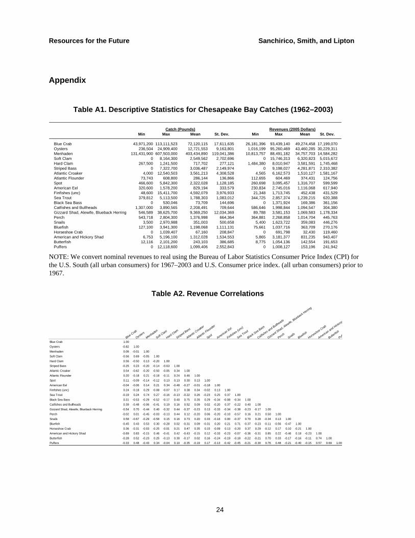
Our species groupings represent a range of aggregation levels, where species aggregations represent a compromise between economic and ecological taxonomy. For instance, blue crab (Callinectes sapidus) is a single species but aggregates across several market categories based on sex, size, and stage of molting (i.e., hard, soft, or peeler). In contrast, there are several species of catfish caught in the Bay (e.g., Ictalurus punctatus and Ictalurus nebulosus), but catch data often do not differentiate among them, and they are necessarily lumped together in our analysis. Some species have separate market categories but are typically caught together or are difficult to distinguish so that catch often is reported in only one species category, e.g. alewife, and blueback herring. Unclassified finfishes are the greatest taxonomic compromise. The category typically contains a variety of small fishes, and although there is no species-specific information for this product category, the category is large enough to meet our economic threshold for inclusion in the analysis. Table A1 (in the appendix) contains descriptive statistics for the 22 species or species groups that meet this criterion.

Because estimates of stock levels or maximum sustainable yield are not available for all 22 fish stocks, we approximate maximum sustainable yield with the observed maximum catch over the period (denoted χi). This assumption implies that for a consistently underutilized species group, the sustainability constraint is overly restrictive, and our analysis precludes recommending an increase in harvest over the historic maximum. This is not a limitation of our method but rather a limitation of the data. If an estimate of MSY is available for an underutilized species k, then we could use it directly for . Nevertheless, we acknowledge that this

assumption is imperfect, and we invoke it here as a starting place for illustrating portfolio management for a real ecosystem. As such, managers should interpret our results with caution. Under these assumptions, the upper bound for each species group in the Bay is

maxkc

cimax(t) = γi(t) χi(t) / Ωi(t). (5)

2 Menhaden are by far the largest catch by volume from the Bay. Menhaden catches for 1985–1996 were obtained from Smith (1999). Estimates of menhaden catches from 1997–2003 and pre-1985 data were obtained from Joseph W. Smith. (NOAA Fisheries, Beaufort, NC, personal communication).

9


We set the sustainability parameter at ½ and 1 for all fish stocks for all periods. For example, γi = γ = ½ indicates a maximum catch equal to one-half the observed maximum catch. The window length (time frame) and weighting scheme over which the maximum catch is calculated varies depending on the specification.

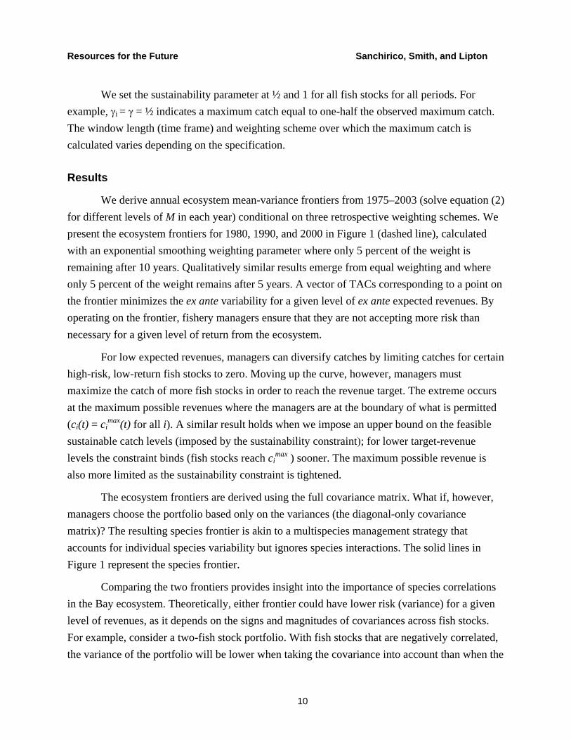
Results

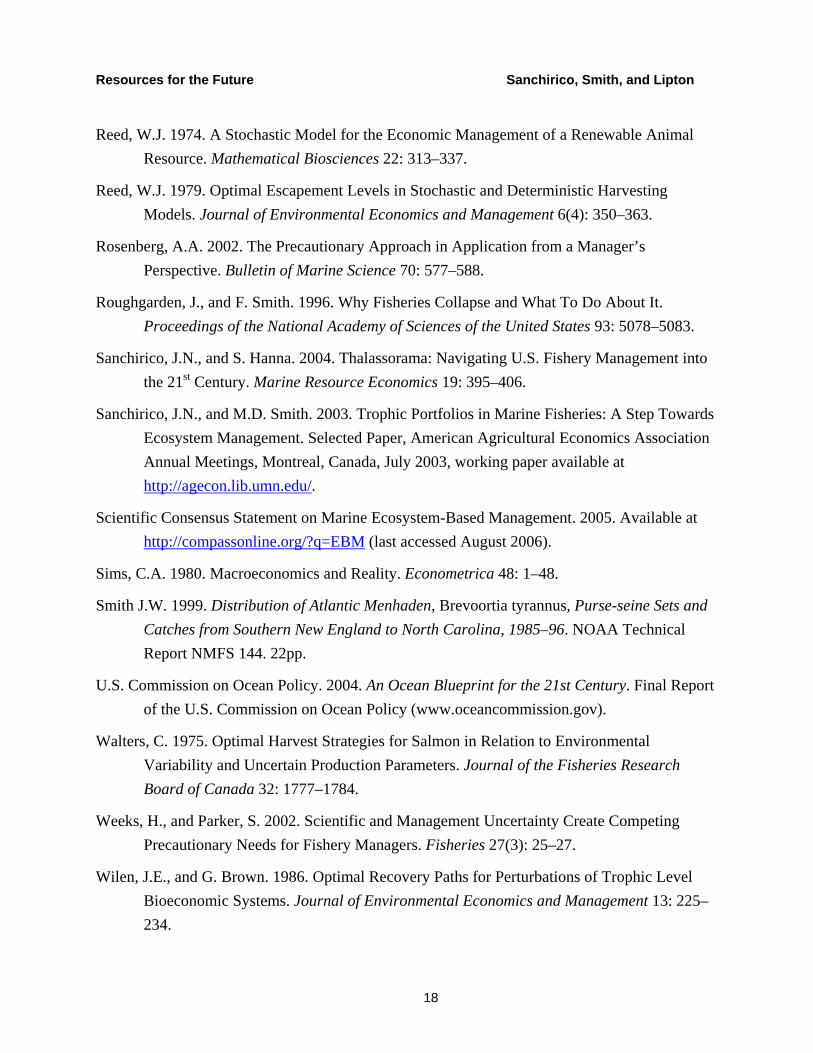
We derive annual ecosystem mean-variance frontiers from 1975–2003 (solve equation (2) for different levels of M in each year) conditional on three retrospective weighting schemes. We present the ecosystem frontiers for 1980, 1990, and 2000 in Figure 1 (dashed line), calculated with an exponential smoothing weighting parameter where only 5 percent of the weight is remaining after 10 years. Qualitatively similar results emerge from equal weighting and where only 5 percent of the weight remains after 5 years. A vector of TACs corresponding to a point on the frontier minimizes the ex ante variability for a given level of ex ante expected revenues. By operating on the frontier, fishery managers ensure that they are not accepting more risk than necessary for a given level of return from the ecosystem.

For low expected revenues, managers can diversify catches by limiting catches for certain high-risk, low-return fish stocks to zero. Moving up the curve, however, managers must maximize the catch of more fish stocks in order to reach the revenue target. The extreme occurs at the maximum possible revenues where the managers are at the boundary of what is permitted (ci(t) = ci

max(t) for all i). A similar result holds when we impose an upper bound on the feasible sustainable catch levels (imposed by the sustainability constraint); for lower target-revenue levels the constraint binds (fish stocks reach ci

max ) sooner. The maximum possible revenue is also more limited as the sustainability constraint is tightened.

The ecosystem frontiers are derived using the full covariance matrix. What if, however, managers choose the portfolio based only on the variances (the diagonal-only covariance matrix)? The resulting species frontier is akin to a multispecies management strategy that accounts for individual species variability but ignores species interactions. The solid lines in Figure 1 represent the species frontier.

Comparing the two frontiers provides insight into the importance of species correlations in the Bay ecosystem. Theoretically, either frontier could have lower risk (variance) for a given level of revenues, as it depends on the signs and magnitudes of covariances across fish stocks. For example, consider a two-fish stock portfolio. With fish stocks that are negatively correlated, the variance of the portfolio will be lower when taking the covariance into account than when the

10


catch shares are derived only with variances. If the fish stocks are positively correlated, however, the ecosystem portfolio could have higher variance than the species case. In an n asset portfolio, the relative portfolio variance depends on the actual covariances of the fish stocks in the portfolio, and we do not have any ex ante reason for either outcome. We find that if managers ignore covariance—ecological and economic interdependence are left out of decisions—then they accept more risk for a given level of revenue. Empirically, this means that there are opportunities to exploit negative covariances across species in the Bay ecosystem.

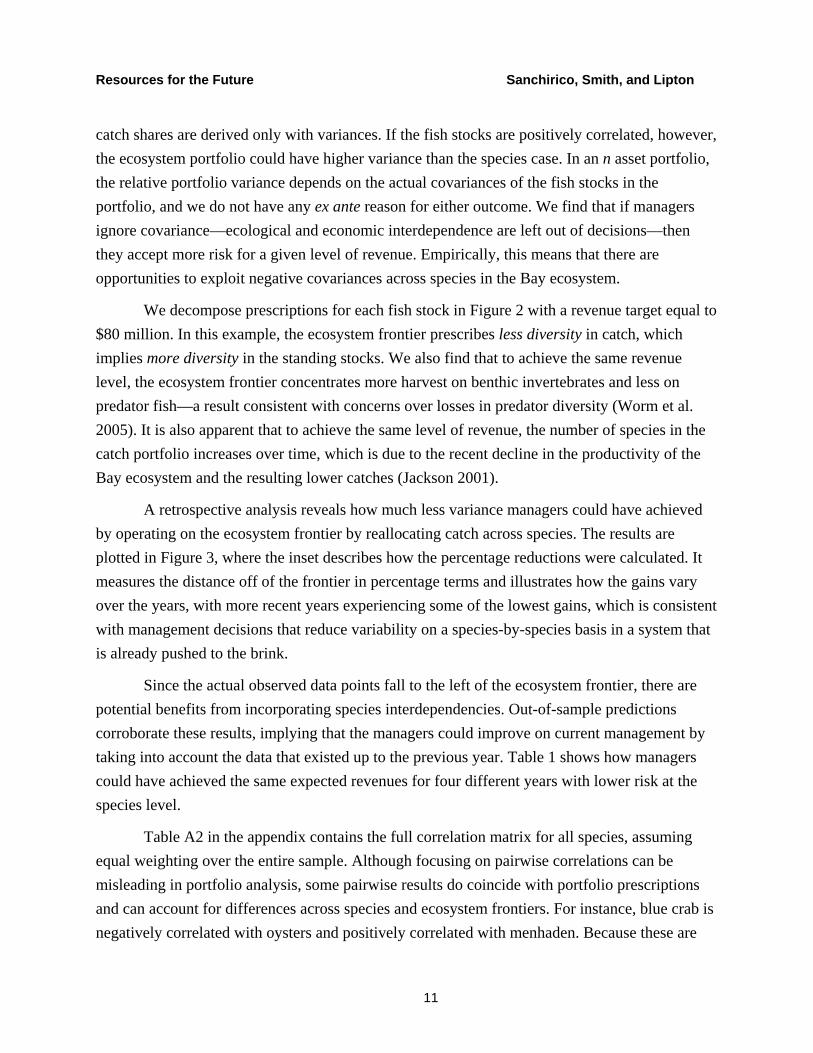
We decompose prescriptions for each fish stock in Figure 2 with a revenue target equal to $80 million. In this example, the ecosystem frontier prescribes less diversity in catch, which implies more diversity in the standing stocks. We also find that to achieve the same revenue level, the ecosystem frontier concentrates more harvest on benthic invertebrates and less on predator fish—a result consistent with concerns over losses in predator diversity (Worm et al. 2005). It is also apparent that to achieve the same level of revenue, the number of species in the catch portfolio increases over time, which is due to the recent decline in the productivity of the Bay ecosystem and the resulting lower catches (Jackson 2001).

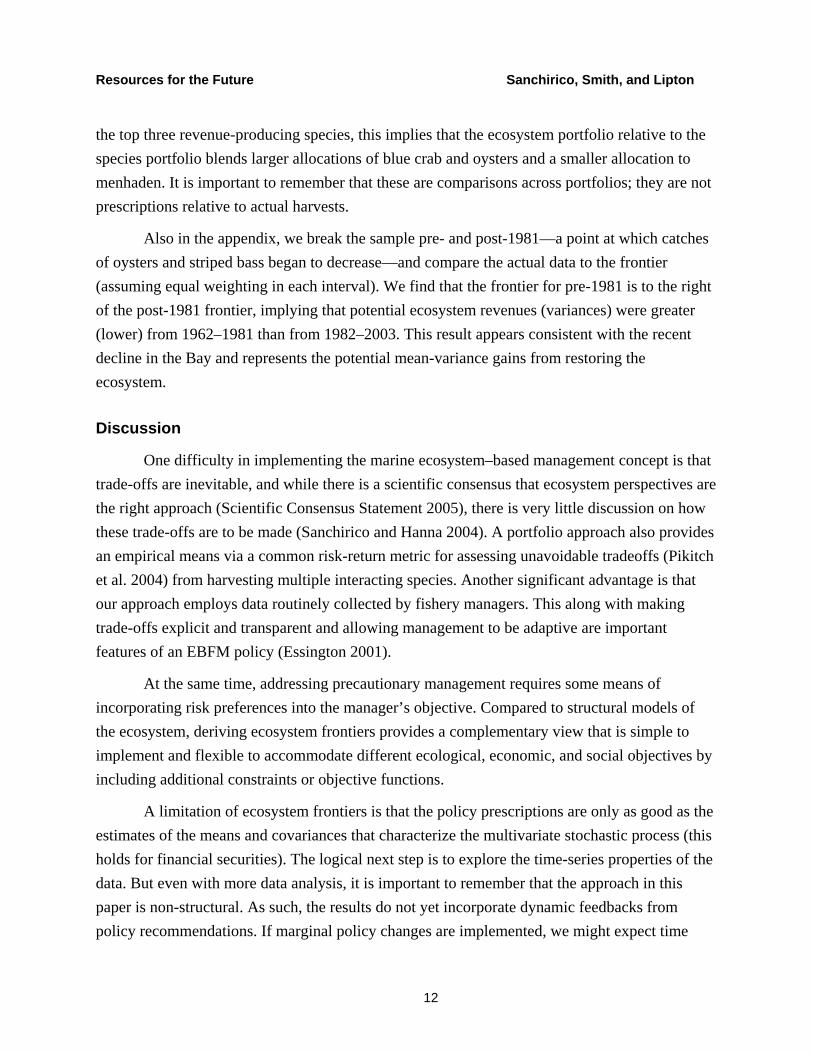
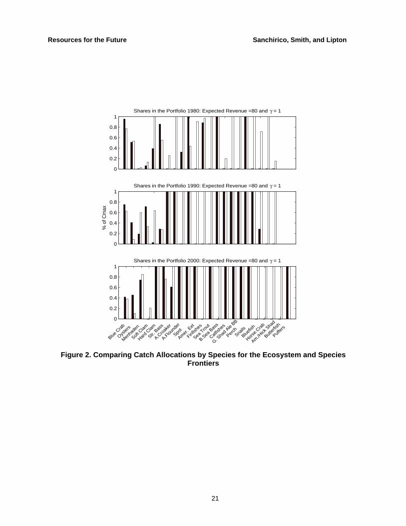
A retrospective analysis reveals how much less variance managers could have achieved by operating on the ecosystem frontier by reallocating catch across species. The results are plotted in Figure 3, where the inset describes how the percentage reductions were calculated. It measures the distance off of the frontier in percentage terms and illustrates how the gains vary over the years, with more recent years experiencing some of the lowest gains, which is consistent with management decisions that reduce variability on a species-by-species basis in a system that is already pushed to the brink.

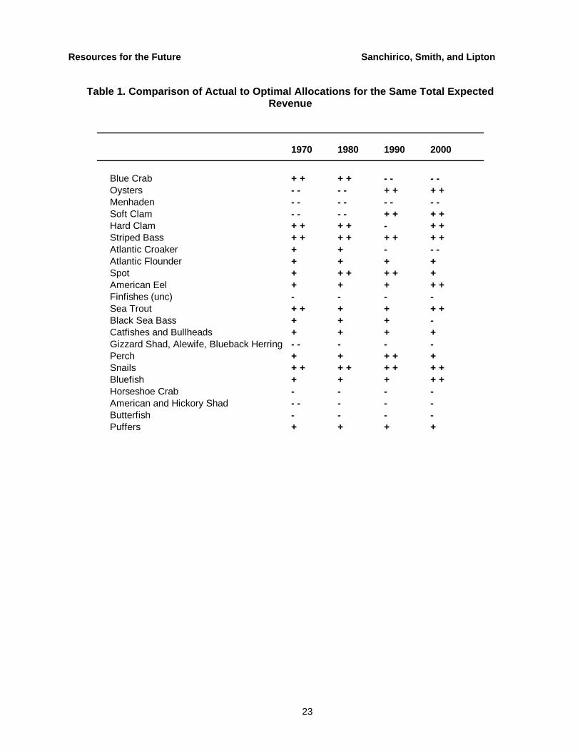
Since the actual observed data points fall to the left of the ecosystem frontier, there are potential benefits from incorporating species interdependencies. Out-of-sample predictions corroborate these results, implying that the managers could improve on current management by taking into account the data that existed up to the previous year. Table 1 shows how managers could have achieved the same expected revenues for four different years with lower risk at the species level.

Table A2 in the appendix contains the full correlation matrix for all species, assuming equal weighting over the entire sample. Although focusing on pairwise correlations can be misleading in portfolio analysis, some pairwise results do coincide with portfolio prescriptions and can account for differences across species and ecosystem frontiers. For instance, blue crab is negatively correlated with oysters and positively correlated with menhaden. Because these are

11


the top three revenue-producing species, this implies that the ecosystem portfolio relative to the species portfolio blends larger allocations of blue crab and oysters and a smaller allocation to menhaden. It is important to remember that these are comparisons across portfolios; they are not prescriptions relative to actual harvests.

Also in the appendix, we break the sample pre- and post-1981—a point at which catches of oysters and striped bass began to decrease—and compare the actual data to the frontier (assuming equal weighting in each interval). We find that the frontier for pre-1981 is to the right of the post-1981 frontier, implying that potential ecosystem revenues (variances) were greater (lower) from 1962–1981 than from 1982–2003. This result appears consistent with the recent decline in the Bay and represents the potential mean-variance gains from restoring the ecosystem.

Discussion

One difficulty in implementing the marine ecosystem–based management concept is that trade-offs are inevitable, and while there is a scientific consensus that ecosystem perspectives are the right approach (Scientific Consensus Statement 2005), there is very little discussion on how these trade-offs are to be made (Sanchirico and Hanna 2004). A portfolio approach also provides an empirical means via a common risk-return metric for assessing unavoidable tradeoffs (Pikitch et al. 2004) from harvesting multiple interacting species. Another significant advantage is that our approach employs data routinely collected by fishery managers. This along with making trade-offs explicit and transparent and allowing management to be adaptive are important features of an EBFM policy (Essington 2001).

At the same time, addressing precautionary management requires some means of incorporating risk preferences into the manager’s objective. Compared to structural models of the ecosystem, deriving ecosystem frontiers provides a complementary view that is simple to implement and flexible to accommodate different ecological, economic, and social objectives by including additional constraints or objective functions.

A limitation of ecosystem frontiers is that the policy prescriptions are only as good as the estimates of the means and covariances that characterize the multivariate stochastic process (this holds for financial securities). The logical next step is to explore the time-series properties of the data. But even with more data analysis, it is important to remember that the approach in this paper is non-structural. As such, the results do not yet incorporate dynamic feedbacks from policy recommendations. If marginal policy changes are implemented, we might expect time

12


series of revenues to continue to convey information signals about the true structural bioeconomic system. But with major policy changes, the time series may have little relevance after a single period of management.

Naturally, before using ecosystem frontiers to guide real-world management decisions, we would like to know how dynamically robust policy prescriptions are. One can only speak to this issue by knowing the true structural model of a system. This suggests two important areas for research. First, in ongoing work, we are exploring the performance of ecosystem frontiers using simulated stochastic bioeconomic systems in which, by construction, we know the true stock dynamics. Second, because a structural ecosystem model of the Bay is under construction using Ecopath with Ecosim, it would be worthwhile to compare policy prescriptions from the structural model with those of the non-structural ecosystem frontiers.

Another extension is to develop ecosystem-based indicators (Brodziak and Link 2002) by measuring the distance between the current state of affairs and the frontier. A similar analysis can be done at the species level. For example, a species may be overfished according to EBFM, but not from the traditional single-species perspective (Pikitch et al. 2004). Knowledge of whether the system is overinvested, fully invested, or underinvested in a species could complement the standard biological measure of overfished, fully exploited, or underfished. An underinvested and overfished resource might be a priority for a recovery plan, as there are gains to increasing its allocation in the portfolio but current population levels limit such an action.

13


References

Annala, John H. 1996. New Zealand's ITQ System: Have the First Eight Years Been a Success or a Failure? Reviews in Fish Biology and Fisheries 6: 43–62

Armsworth, P., and J. Roughgarden. 2003. The Economic Value of Ecological Stability. Proceedings of the National Academy of Sciences of the United States 100(12): 7147–7151.

Arnason, R. 1998. Ecological Fisheries Management Using Individual Transferable Share Quotas. Ecological Applications 8: S151–S159.

Baldursson, F.M., and G. Magnusson. 1997. Portfolio Fishing. Scandinavian Journal of Economics 99(3): 389–403.

Bascompte, J., C.J. Melian, and E. Sala. 2003. Interaction Strength Combinations and the Overfishing of a Marine Food Web. Proceedings of the National Academy of Sciences of the United States 102(15): 5443–5447.

Bollerslev, T. 1986. Generalized Autoregressive Conditional Heteroskedasticity. Journal of Econometrics 31: 307–327.

Botsford, Louis W., Juan Carlos Castilla, Charles H. Peterson. 1997. The Management of Fisheries and Marine Ecosystems. Science 277: 509–515.

Brodziak, J., and J. Link. 2002. Ecosystem-based Fishery Management: What It Is and How Can We Do It? Bulletin of Marine Science 70: 589–612.

Charles, A.T. 2002. The Precautionary Approach and ‘Burden of Proof’ Challenges in Fishery Management. Bulletin of Marine Science 70: 683–694.

Chesapeake Bay Commission. 2006. Blue Crab 2005: Status of the Chesapeake Population and Its Fisheries. Annapolis, MD: Bi-State Blue Crab Technical Advisory Committee.

Christensen, V., and C. J. Walters. 2004. Ecopath with Ecosim: Methods, Capabilities, and Limitations. Ecological Modeling 172: 109–139.

Clark, C.W. 1990. Mathematical Bioeconomics: The Optimal Management of Renewable Resources, 2nd Edition. New York: John Wiley & Sons, Inc.

Clark, C.W., and G.R. Munro. 1975. The Economics of Fishing and Modern Capital Theory: A Simplified Approach. Journal of Environmental Economics and Management 2: 92–106.

14


Dame, J.K., and R.R. Christian. 2006. Uncertainty and the Use of Network Analysis for Ecosystem-based Fishery Management. Fisheries 31(7): 331–341.

Darcy, G.H., and G.C. Matlock. 1999. Application of the Precautionary Approach in the National Standard Guidelines for Conservation and Management of Fisheries in the United States. ICES Journal of Marine Science 56: 853–859.

Edwards, S.F., J.S. Link, and B.P. Rountree. 2004. Portfolio Management of Wild Fish Stocks. Ecological Economics 49: 317–329.

Engle, R.F., and C. Granger. 1987. Co-Integration and Error Correction: Representation, Estimation, and Testing. Econometrica 55: 251–76.

Essington, T. 2001. Precautionary approach in Fisheries Management: The Devil Is in the Details. Trends in Ecology and Evolution 13: 121–122.

Essington, T. 2004. Getting the Right Answer from the Wrong Model: Evaluating the Sensitivity of Multi-Species Fisheries Advice to Uncertain Species Interactions. Bulletin of Marine Science 74(3):563–581.

Essington, T.E., A.H. Beaudreau, and J. Wiedenmann. 2006. Fishing through Marine Food Webs. Proceedings of the National Academy of Sciences of the United States 103: 3171–3175.

Finnoff, D., and J. Tschirhart. 2003. Harvesting in an Eight-species Ecosystem. Journal of Environmental Economics and Management 45(3): 589–611.

Fulton, E., A. Smith, and C. R. Johnson. 2003. Effect of Complexity on Marine Ecosystem Models. Marine Ecology Progress Series 253: 1–16.

Garcia, S.M. 1994. The Precautionary Principle: Its Implications in Capture Fisheries Management. Ocean and Coastal Management 22: 99–125.

Gerrodette, T., P.K. Dayton, S. Macinko, and M.J. Fogarty. 2002. Precautionary Management of Marine Fisheries: Moving Beyond Burden of Proof. Bulletin of Marine Science 70: 657–668.

Hanna, S. 1998. Institutions for Marine Ecosystems: Economic Incentives and Fishery Management. Ecological Applications 8: S170–S174.

Hannesson, R. 1983. Optimal Harvesting of Ecologically Interdependent Fish Species. Journal of Environmental Economics and Management 10: 329–45.

15


Hildebrand S.F., and W.C. Schroeder. 1928. Fishes of the Chesapeake Bay. United States Bureau of Fisheries Bulletin 53(1). (reprinted 1972). 388pp.

Hilborn, R., J-J. Maguire, A.M. Parma, and A.A. Rosenberg. 2001. The Precautionary Approach and Risk Management: Can They Increase the Probability of Successes in Fishery Management? Canadian Journal of Fisheries and Aquatic Sciences 58: 99–107.

Hofmann, E.E., and T.M. Powell. 1998. Environmental Variability Effects on Marine Fisheries: Four Case Histories. Ecological Applications 8: S23–S32.

Houde, E.D., M.J. Fogarty, and T.J. Miller. 1998. Prospects for Multispecies Fisheries Management in Chesapeake Bay: A Workshop. STAC Publication 98-002.

JP Morgan/Reuters. 1996. RiskMetrics—Technical Document, 4th Edition. New York: Morgan Guaranty Trust Company and Reuters Ltd.

Jackson, Jeremy B. C., Michael X. Kirby, Wolfgang H. Berger, Karen A. Bjorndal, Louis W. Botsford, Bruce J. Bourque, Roger H. Bradbury, Richard Cooke, Jon Erlandson, James A. Estes, Terence P. Hughes, Susan Kidwell, Carina B. Lange, Hunter S. Lenihan, John M. Pandolfi, Charles H. Peterson, Robert S. Steneck, Mia J. Tegner, Robert R. Warner. 2001. Historical Overfishing and the Recent Collapse of Coastal Ecosystems. Science 293: 629–637.

Jackson, Jeremy. 2001. What Was Natural in Coastal Oceans? Proceedings of the National Academy of Sciences of the United States 98(10): 5411–5418.

Lauck, T.C., C.W. Clark, M. Mangel, and G.R. Munro. 1998. Implementing the Precautionary Principle in Fisheries Management Through Marine Reserves. Ecological Applications 8(1): S72–S78.

Lipcius, R.N., R.D. Seitz, W.J. Goldsborough, M.M. Montane, and W.T. Stockhausen. 2001. A Deep-water Dispersal Corridor for Adult Female Blue Crabs in Chesapeake Bay. In Spatial Processes and Management of Marine Populations (Gordon H. Kruse, Nicolas Bez, Anthony Booth, Martin W. Dorn, Sue Hills, Romuald N. Lipcius, Dominique Pelletier, Claude Roy, Stephen J. Smith, and David Witherell, eds.). Fairbanks: University of Alaska Sea Grant, AK-SG-01-02, 643–666.

Lipton, D.W., E.F. Lavan, and I.E. Strand. 1992. Economics of Molluscan Introductions and Transfers: The Chesapeake Bay Dilemma. Journal of Shellfish Research 11(2): 511–519.

16


Ludwig, D. 2002. A Quantitative Precautionary Approach. Bulletin of Marine Science 70: 485–497.

Markowitz, H. 1952. Portfolio Selection. Journal of Finance VII(1): 77–91, 1952.

McAllister, M., and C. Kirchner. 2002. Accounting for Structural Uncertainty to Facilitate Precautionary Fishery Management: Illustration with Namibian Orange Roughy. Bulletin of Marine Science 70: 499–540.

Myers, R.A., and G. Mertz. 1998. The Limits of Exploitation: A Precautionary Approach. Ecological Applications 8: S165–S169.

NOAA Fisheries. 2006. 2005 Report of Status of Fisheries. http://www.nmfs.noaa.gov/sfa/domes_fish/ReportsToCongress/finalSOS/Report_text_FINAL3.pdf.

Paolisso, M. 2002. Blue Crabs and Controversy on the Chesapeake Bay: A Cultural Model for Understanding Watermen’s Reasoning about Blue Crab Management. Human Organization 61(3): 2236–239.

Pauly, D., V. Christensen, J. Dalsgaard, R. Froese, and F. Torres, Jr. 1998. Fishing Down Marine Food Webs. Science 279: 860–863.

Perusso, L., R.N. Weldon, and S.L. Larkin. 2005. Predicting Optimal Targeting Strategies in Multispecies Fisheries: A Portfolio Approach. Marine Resource Economics 20(1): 25–45.

Pew Oceans Commission. 2003. America's Living Oceans: Charting a Course for Sea Change. A Report to the Nation. Arlington, VA: Pew Oceans Commission.

Pikitch, E. K., C. Santora, E.A. Babcock, A. Bakun, R. Bonfil, D.O. Conover, P. Dayton, P. Doukakis, D. Fluharty, B. Heneman, E.D. Houde, J. Link, P.A. Livingston, M. Mangel, M.K. McAllister, J. Pope, and K.J. Sainsbury. 2004. ECOLOGY: Ecosystem-Based Fishery Management. Science 305: 346–347.

Quirk, J.P., and V.L. Smith. 1970. Dynamic Economic Models of Fishing. In Economics of Fisheries Management: A Symposium (A.D. Scott, ed.). H. R. McMillan Lectures in Fisheries. Vancouver: University of British Columbia.

Ragozin, D.L., and G. Brown. 1985. Harvest Policies and Nonmarket Valuation in a Predator-Prey System. Journal of Environmental Economics and Management 12: 155–168.

Real, L.A. 1991. Animal Choice Behavior and the Evolution of Cognitive Architecture. Science 253: 980–986.

17


Reed, W.J. 1974. A Stochastic Model for the Economic Management of a Renewable Animal Resource. Mathematical Biosciences 22: 313–337.

Reed, W.J. 1979. Optimal Escapement Levels in Stochastic and Deterministic Harvesting Models. Journal of Environmental Economics and Management 6(4): 350–363.

Rosenberg, A.A. 2002. The Precautionary Approach in Application from a Manager’s Perspective. Bulletin of Marine Science 70: 577–588.

Roughgarden, J., and F. Smith. 1996. Why Fisheries Collapse and What To Do About It. Proceedings of the National Academy of Sciences of the United States 93: 5078–5083.

Sanchirico, J.N., and S. Hanna. 2004. Thalassorama: Navigating U.S. Fishery Management into the 21st Century. Marine Resource Economics 19: 395–406.

Sanchirico, J.N., and M.D. Smith. 2003. Trophic Portfolios in Marine Fisheries: A Step Towards Ecosystem Management. Selected Paper, American Agricultural Economics Association Annual Meetings, Montreal, Canada, July 2003, working paper available at http://agecon.lib.umn.edu/.

Scientific Consensus Statement on Marine Ecosystem-Based Management. 2005. Available at http://compassonline.org/?q=EBM (last accessed August 2006).

Sims, C.A. 1980. Macroeconomics and Reality. Econometrica 48: 1–48.

Smith J.W. 1999. Distribution of Atlantic Menhaden, Brevoortia tyrannus, Purse-seine Sets and Catches from Southern New England to North Carolina, 1985–96. NOAA Technical Report NMFS 144. 22pp.

U.S. Commission on Ocean Policy. 2004. An Ocean Blueprint for the 21st Century. Final Report of the U.S. Commission on Ocean Policy (www.oceancommission.gov).

Walters, C. 1975. Optimal Harvest Strategies for Salmon in Relation to Environmental Variability and Uncertain Production Parameters. Journal of the Fisheries Research Board of Canada 32: 1777–1784.

Weeks, H., and Parker, S. 2002. Scientific and Management Uncertainty Create Competing Precautionary Needs for Fishery Managers. Fisheries 27(3): 25–27.

Wilen, J.E., and G. Brown. 1986. Optimal Recovery Paths for Perturbations of Trophic Level Bioeconomic Systems. Journal of Environmental Economics and Management 13: 225–234.

18

http://agecon.lib.umn.edu/

http://compassonline.org/?q=EBM

http://www.oceancommission.gov/documents/full_color_rpt/000_ocean_full_report.pdf


Worm, B., M. Sandow, A. Oschlies, H.K. Lotze, and R.A. Myers. 2005. Global Patterns of Predator Diversity in the Open Oceans. Science 309: 1365–1369.

19


Figures and Tables

0 50 1000

20

40

60

801980 γ = 1/2

0 20 40 60 800

20

40

60

80

Var

ianc

e (T

rillio

ns)

1990 γ = 1/2

0 20 40 60 800

20

40

60

Expected Revenues (Millions $)

2000 γ = 1/2

0 50 100 150 2000

100

200

300

4001980 γ = 1

0 50 100 150 2000

100

200

300

4001990 γ = 1

0 50 100 1500

50

100

150

200

250

Expected Revenues (Millions $)

2000 γ = 1

Figure 1. Efficient Frontiers for Two Levels of γ

20


0

0.2

0.4

0.6

0.8

1Shares in the Portfolio 1980: Expected Revenue =80 and γ = 1

0

0.2

0.4

0.6

0.8


% o

f Cm

ax

0

0.2

0.4

0.6

0.8


Blue C

rab

Oyster

s

Menha

den

Soft C

lam

Hard C

lam

Str. B

ass

A.Cro

aker

A.Flou

nder

Spot

Amer. E

el

Finfish

es

Sea T

rout

B.Sea

Bas

s

Catfish

es

G. Sha

d Ale

BB

Perch

Snails

Bluefis

h

Horse

.Cra

b

Am./Hick

Sha

d

Butter

fish

Puffer

s

Figure 2. Comparing Catch Allocations by Species for the Ecosystem and Species

Frontiers

21


0 2 4 6 8 10 12 14 16−60

−50

−40

−30

−20

−10

0

1976

1977

19781979

1980

1981

1982

1983

1984

1985

1986

1987

1988

1989

1990

1991

1992

1993

1994

1995

19961997

1998

1999

2000

20012002

Additional Revenue (% of actual)

Red

uctio

n in

Var

ianc

e (%

of a

ctua

l)Percentage gains from operating on the ecosystem frontier

actual

∆ R| v = va

∆ V | r = ra

Revenue

Var

ianc

e

Figure 3. Comparison of Actual Management to Efficient Frontiers

22


Table 1. Comparison of Actual to Optimal Allocations for the Same Total Expected Revenue

1970 1980 1990 2000

Blue Crab + + + + - - - -Oysters - - - - + + + +Menhaden - - - - - - - -Soft Clam - - - - + + + +Hard Clam + + + + - + +Striped Bass + + + + + + + +Atlantic Croaker + + - - -Atlantic Flounder + + + +Spot + + + + + +American Eel + + + + +Finfishes (unc) - - - -Sea Trout + + + + + +Black Sea Bass + + + -Catfishes and Bullheads + + + +Gizzard Shad, Alewife, Blueback Herring - - - - -Perch + + + + +Snails + + + + + + + +Bluefish + + + + +Horseshoe Crab - - - -American and Hickory Shad - - - - -Butterfish - - - -Puffers + + + +

23


Appendix

Table A1. Descriptive Statistics for Chesapeake Bay Catches (1962–2003)

Catch (Pounds) Revenues (2005 Dollars)Min Max Mean St. Dev. Min Max Mean St. Dev.

Blue Crab 43,971,200 113,111,523 72,120,115 17,611,635 26,181,396 93,439,140 49,274,458 17,199,070Oysters 236,504 24,909,400 12,721,553 9,163,801 1,016,199 95,260,469 43,460,285 30,229,311Menhaden 131,431,900 607,503,000 403,434,890 119,041,386 10,813,757 88,491,182 34,757,703 14,584,282Soft Clam 0 8,164,300 2,549,562 2,702,696 0 15,746,313 6,320,823 5,015,672Hard Clam 267,500 1,241,500 717,702 277,121 1,484,380 8,010,947 3,581,591 1,745,468Striped Bass 0 7,322,700 3,036,487 2,149,974 0 9,198,027 4,281,871 2,310,382Atlantic Croaker 4,000 12,540,503 3,561,213 4,308,528 4,565 6,162,573 1,510,127 1,581,167Atlantic Flounder 73,743 608,800 286,144 136,866 112,655 604,469 374,431 124,756Spot 466,600 5,842,300 2,322,028 1,128,185 260,698 3,095,457 1,316,707 599,599American Eel 320,600 1,578,200 829,194 333,579 230,834 2,745,016 1,116,068 617,940Finfishes (unc) 48,600 15,411,700 4,592,079 3,976,933 21,348 1,713,745 452,438 431,529Sea Trout 379,812 5,113,500 1,788,303 1,083,012 344,725 2,857,374 1,239,215 620,388Black Sea Bass 0 530,046 73,709 144,696 0 1,371,924 169,386 361,156Catfishes and Bullheads 1,307,000 3,890,565 2,208,491 709,644 586,646 1,998,844 1,094,547 304,380Gizzard Shad, Alewife, Blueback Herring 546,589 38,625,700 9,369,250 12,034,369 89,788 3,581,153 1,069,583 1,178,334Perch 543,718 2,804,300 1,376,998 664,364 364,881 2,268,858 1,014,704 445,763Snails 3,500 2,970,988 351,003 500,658 5,400 1,623,722 359,083 446,276Bluefish 127,100 3,941,300 1,198,068 1,111,131 75,661 1,037,716 363,709 270,176Horseshoe Crab 0 1,039,407 67,160 208,847 0 691,798 32,430 119,460American and Hickory Shad 6,753 5,196,100 1,312,028 1,534,553 5,865 3,181,377 831,235 943,407Butterfish 12,116 2,101,200 243,103 386,685 8,775 1,054,136 142,554 191,653Puffers 0 12,118,600 1,099,406 2,552,843 0 1,008,127 153,196 241,942

NOTE: We convert nominal revenues to real using the Bureau of Labor Statistics Consumer Price Index (CPI) for the U.S. South (all urban consumers) for 1967–2003 and U.S. Consumer price index. (all urban consumers) prior to 1967.

Table A2. Revenue Correlations

Blue Crab

Oysters

Menhaden

Soft Clam

Hard Clam

Striped Bass

Atlantic Croaker

Atlantic Flounder

SpotAmerican Eel

Finfishes (u

nc)

Sea Trout

Black Sea Bass

Catfishes and Bullheads

Gizzard Shad, Alewife, B

lueback Herring

PerchSnails

Bluefish

Horseshoe Crab

American and Hickory S

Butterfish

Puff

Blue Crab 1.00Oysters -0.82 1.00Menhaden 0.06 -0.01 1.00Soft Clam -0.56 0.69 -0.05 1.00Hard Clam 0.56 -0.50 0.13 -0.20 1.00Striped Bass -0.25 0.23 -0.20 -0.14 -0.63 1.00Atlantic Croaker 0.54 -0.62 -0.20 -0.50 -0.05 0.34 1.00Atlantic Flounder 0.20 -0.18 0.21 -0.18 -0.11 0.24 0.46 1.00Spot 0.11 -0.09 -0.14 -0.12 0.13 0.13 0.30 0.13 1.00American Eel -0.04 -0.06 0.14 0.21 0.34 -0.48 -0.27 -0.01 -0.18 1.00Finfishes (unc) 0.24 -0.18 0.29 -0.08 -0.07 0.17 0.38 0.34 -0.02 0.13 1.00Sea Trout -0.19 0.24 0.74 0.27 -0.16 -0.13 -0.22 0.26 -0.23 0.25 0.37 1.00Black Sea Bass 0.31 -0.53 -0.29 -0.52 -0.17 0.40 0.75 0.26 0.29 -0.34 -0.08 -0.34 1.00Catfishes and Bullheads 0.39 -0.48 -0.06 -0.41 0.19 0.16 0.52 0.09 0.02 -0.20 0.37 -0.22 0.40 1.00Gizzard Shad, Alewife, Blueback Herring -0.54 0.70 -0.44 0.40 -0.32 0.44 -0.37 -0.23 0.13 -0.33 -0.34 -0.38 -0.23 -0.17 1.00Perch -0.02 0.01 -0.45 -0.03 -0.13 0.44 0.12 -0.20 0.06 -0.20 -0.10 -0.57 0.16 0.21 0.50 1.00Snails 0.58 -0.67 -0.29 -0.58 0.15 0.16 0.73 0.20 0.33 -0.16 0.00 -0.37 0.70 0.28 -0.34 0.13 1.00Bluefish -0.45 0.43 0.53 0.30 -0.28 0.02 -0.31 0.09 -0.31 0.20 0.21 0.71 -0.37 -0.23 -0.11 -0.56 -0.47 1.00Horseshoe Crab 0.36 -0.31 -0.03 -0.25 -0.01 0.21 0.47 0.35 0.15 -0.09 0.13 -0.20 0.37 0.29 -0.12 0.17 0.10 -0.21 1.00American and Hickory Shad -0.69 0.83 -0.15 0.46 -0.41 0.42 -0.43 -0.15 0.12 -0.33 -0.23 -0.07 -0.36 -0.31 0.85 0.22 -0.46 0.18 -0.23 1.00Butterfish -0.28 0.52 -0.23 0.25 -0.13 0.30 -0.17 0.02 0.16 -0.24 -0.19 -0.18 -0.22 -0.21 0.70 0.33 -0.17 -0.16 -0.11 0.74 1.00Puffers -0.33 0.48 -0.43 0.34 -0.04 0.10 -0.35 -0.19 0.17 -0.13 -0.42 -0.45 -0.21 -0.30 0.76 0.48 -0.21 -0.40 -0.15 0.57 0.69 1.00

24


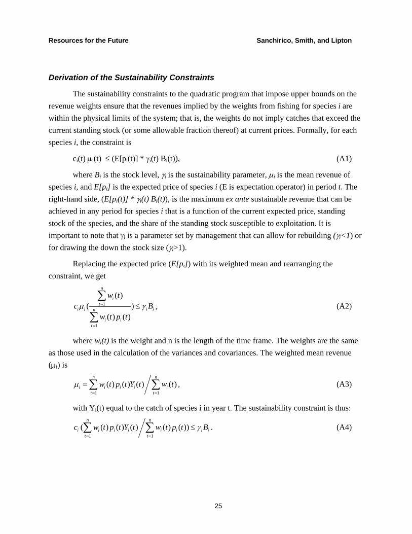
Derivation of the Sustainability Constraints

The sustainability constraints to the quadratic program that impose upper bounds on the revenue weights ensure that the revenues implied by the weights from fishing for species i are within the physical limits of the system; that is, the weights do not imply catches that exceed the current standing stock (or some allowable fraction thereof) at current prices. Formally, for each species i, the constraint is

ci(t) µi(t) ≤ (E[pi(t)] * γi(t) Bi(t)), (A1)

where Bi is the stock level, γi is the sustainability parameter, µi is the mean revenue of species i, and E[pi] is the expected price of species i (E is expectation operator) in period t. The right-hand side, (E[pi(t)] * γi(t) Bi(t)), is the maximum ex ante sustainable revenue that can be achieved in any period for species i that is a function of the current expected price, standing stock of the species, and the share of the standing stock susceptible to exploitation. It is important to note that γi is a parameter set by management that can allow for rebuilding (γi<1) or for drawing the down the stock size (γi>1).

Replacing the expected price (E[pi]) with its weighted mean and rearranging the constraint, we get

1

1

( )( )

( ) ( )

n

it

i i i in

i it

w tc B

w t p tµ γ=

=

≤∑

∑, (A2)

where wi(t) is the weight and n is the length of the time frame. The weights are the same as those used in the calculation of the variances and covariances. The weighted mean revenue (µi) is

1 1( ) ( ) ( ) ( )

n n

i i i i it t

w t p t Y t w tµ= =

= ∑ ∑ , (A3)

with Yi(t) equal to the catch of species i in year t. The sustainability constraint is thus:

1 1

( ( ) ( ) ( ) ( ) ( ))n n

i i i i i i it t

c w t p t Y t w t p t Biγ= =

≤∑ ∑ . (A4)

25


From equation (A4), the scaling factor is defined as:

1 1( ( ) ( ) ( ) ( ) ( ))

n n

i i i i i it t

w t p t Y t w t p t= =

Ω ≡ ∑ ∑ , (A5)

which is a weighted average of catches.

Comparing Actual to Efficient Allocations

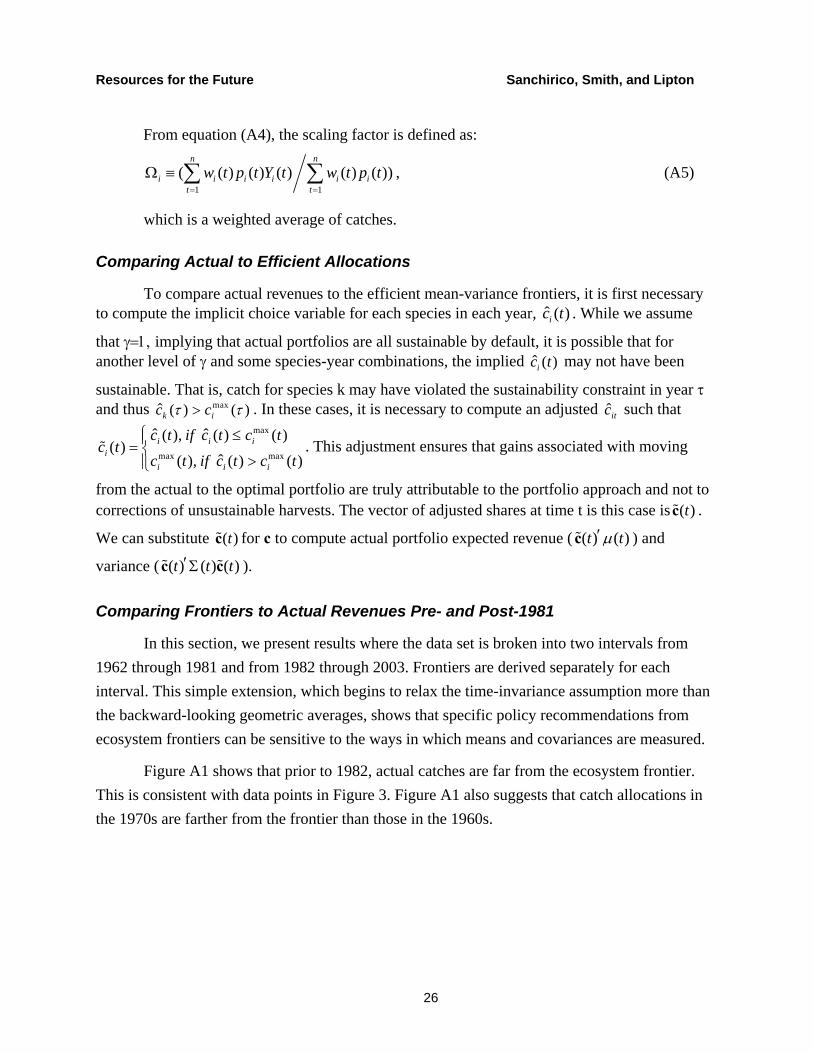
To compare actual revenues to the efficient mean-variance frontiers, it is first necessary to compute the implicit choice variable for each species in each year, . While we assume

that γ=1, implying that actual portfolios are all sustainable by default, it is possible that for another level of γ and some species-year combinations, the implied may not have been

sustainable. That is, catch for species k may have violated the sustainability constraint in year τ and thus

ˆ ( )ic t

ˆ ( )ic t

maxˆ ( ) ( )k ic cτ τ> . In these cases, it is necessary to compute an adjusted such that ˆitcmax

max max

ˆ ˆ( ), ( ) ( )( )

ˆ( ), ( ) ( )i i i

ii i i

c t if c t c tc t

c t if c t c t

⎧ ≤⎪= ⎨>⎪⎩

% . This adjustment ensures that gains associated with moving

from the actual to the optimal portfolio are truly attributable to the portfolio approach and not to corrections of unsustainable harvests. The vector of adjusted shares at time t is this case is .

We can substitute for c to compute actual portfolio expected revenue (

( )tc%

( )tc% ( ) ( )t tµ′c% ) and

variance ( ). ( ) ( ) ( )t t t′Σc c% %

Comparing Frontiers to Actual Revenues Pre- and Post-1981

In this section, we present results where the data set is broken into two intervals from 1962 through 1981 and from 1982 through 2003. Frontiers are derived separately for each interval. This simple extension, which begins to relax the time-invariance assumption more than the backward-looking geometric averages, shows that specific policy recommendations from ecosystem frontiers can be sensitive to the ways in which means and covariances are measured.

Figure A1 shows that prior to 1982, actual catches are far from the ecosystem frontier. This is consistent with data points in Figure 3. Figure A1 also suggests that catch allocations in the 1970s are farther from the frontier than those in the 1960s.

26


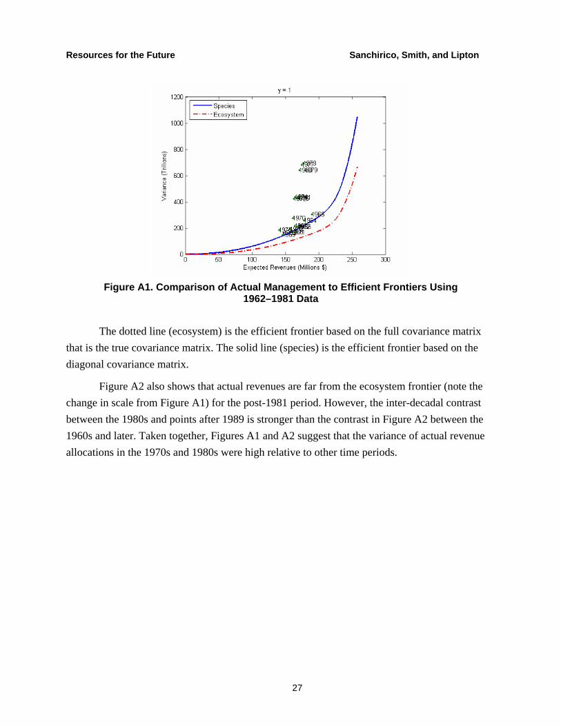
Figure A1. Comparison of Actual Management to Efficient Frontiers Using

1962–1981 Data

The dotted line (ecosystem) is the efficient frontier based on the full covariance matrix that is the true covariance matrix. The solid line (species) is the efficient frontier based on the diagonal covariance matrix.

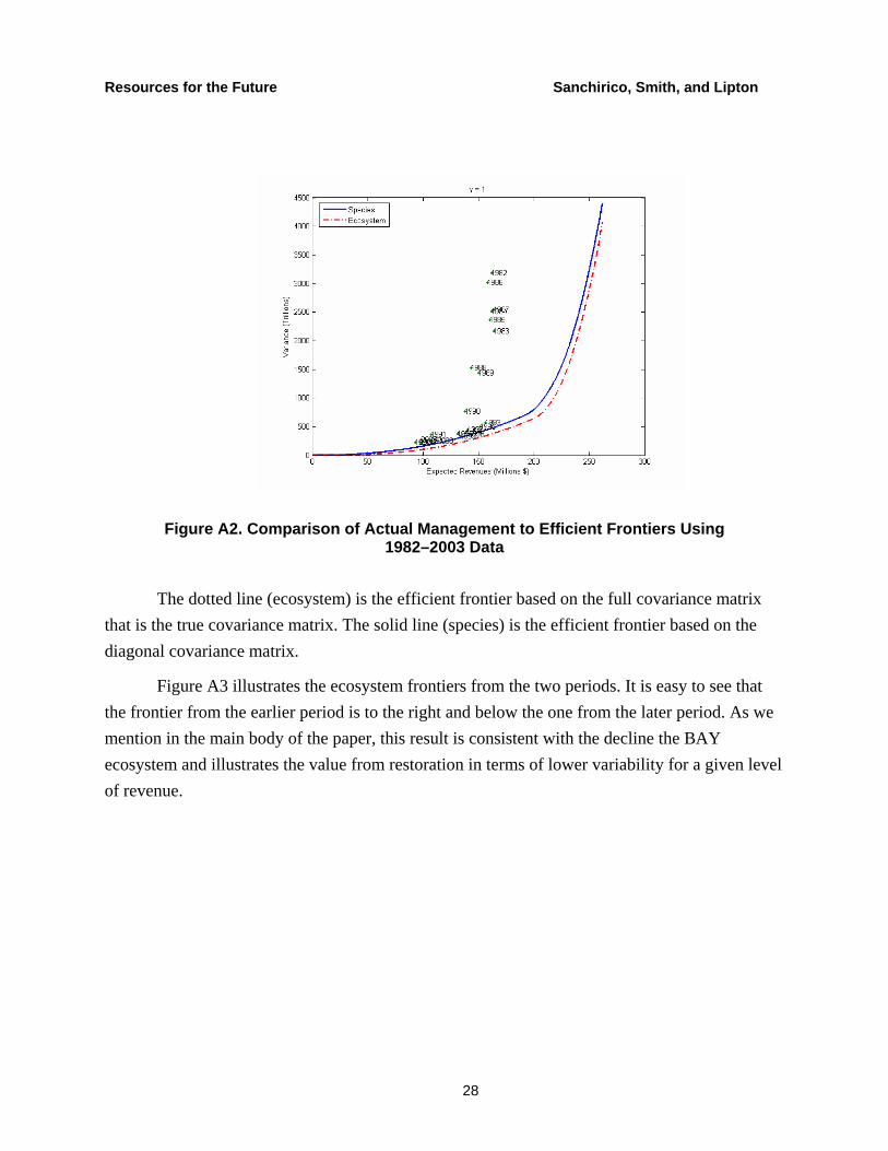
Figure A2 also shows that actual revenues are far from the ecosystem frontier (note the change in scale from Figure A1) for the post-1981 period. However, the inter-decadal contrast between the 1980s and points after 1989 is stronger than the contrast in Figure A2 between the 1960s and later. Taken together, Figures A1 and A2 suggest that the variance of actual revenue allocations in the 1970s and 1980s were high relative to other time periods.

27


Figure A2. Comparison of Actual Management to Efficient Frontiers Using 1982–2003 Data

The dotted line (ecosystem) is the efficient frontier based on the full covariance matrix that is the true covariance matrix. The solid line (species) is the efficient frontier based on the diagonal covariance matrix.

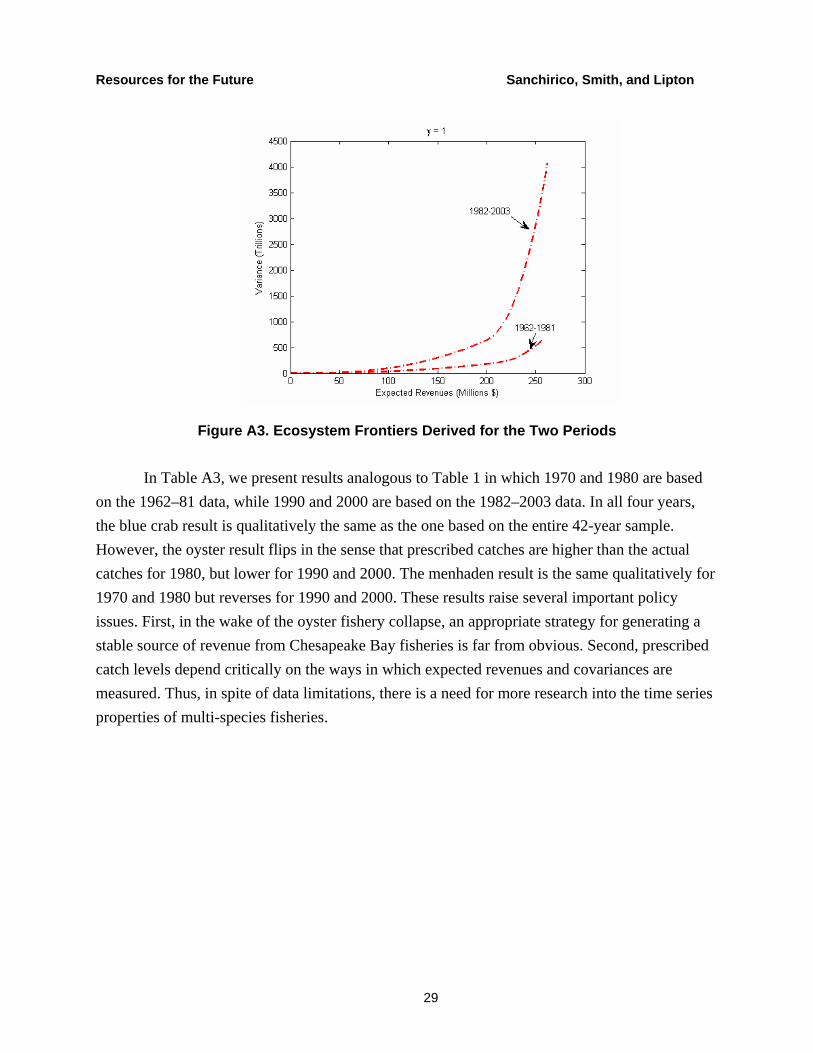
Figure A3 illustrates the ecosystem frontiers from the two periods. It is easy to see that the frontier from the earlier period is to the right and below the one from the later period. As we mention in the main body of the paper, this result is consistent with the decline the BAY ecosystem and illustrates the value from restoration in terms of lower variability for a given level of revenue.

28


Figure A3. Ecosystem Frontiers Derived for the Two Periods

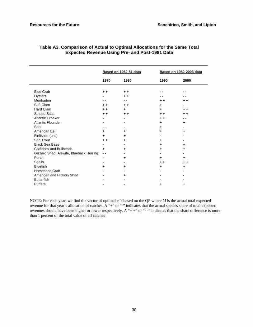
In Table A3, we present results analogous to Table 1 in which 1970 and 1980 are based on the 1962–81 data, while 1990 and 2000 are based on the 1982–2003 data. In all four years, the blue crab result is qualitatively the same as the one based on the entire 42-year sample. However, the oyster result flips in the sense that prescribed catches are higher than the actual catches for 1980, but lower for 1990 and 2000. The menhaden result is the same qualitatively for 1970 and 1980 but reverses for 1990 and 2000. These results raise several important policy issues. First, in the wake of the oyster fishery collapse, an appropriate strategy for generating a stable source of revenue from Chesapeake Bay fisheries is far from obvious. Second, prescribed catch levels depend critically on the ways in which expected revenues and covariances are measured. Thus, in spite of data limitations, there is a need for more research into the time series properties of multi-species fisheries.

29


Table A3. Comparison of Actual to Optimal Allocations for the Same Total Expected Revenue Using Pre- and Post-1981 Data

Based on 1962-81 data Based on 1982-2003 data

1970 1980 1990 2000

Blue Crab + + + + - - - -Oysters - + + - - - -Menhaden - - - - + + + +Soft Clam + + + + + -Hard Clam + + + + + +Striped Bass + + + + + + + +Atlantic Croaker - - + + - -Atlantic Flounder - - + +Spot - - - + -American Eel + + + +Finfishes (unc) + + - -Sea Trout + + + + -Black Sea Bass - - + +Catfishes and Bullheads + + + +Gizzard Shad, Alewife, Blueback Herring - - - - -Perch - + + +Snails - - + + + +Bluefish + + + +Horseshoe Crab - - - -American and Hickory Shad - + - -Butterfish - - - -Puffers - - + +

NOTE: For each year, we find the vector of optimal ci’s based on the QP where M is the actual total expected revenue for that year’s allocation of catches. A “+” or “-” indicates that the actual species share of total expected revenues should have been higher or lower respectively. A “+ +” or “- -” indicates that the share difference is more than 1 percent of the total value of all catches

30

Documents

An Approach to Ecosystem-Based Fishery Managementbiology.kenyon.edu/courses/envs461/0321 Ecosystem...As a complement to constant escapement and structural ecosystem models, we propose