Embed Size (px)
Citation preview
An Approach To Publish a Data Warehouse Content as Linked Data
António Miguel Torres Dourado
Dissertation to obtain the Master of Science degree in
Computer Science, Specialization in
Knowledge-based and Decision Support Technologies
Orientador: Paulo Maio
Co-orientador: Nuno Silva
Júri:
Presidente:
Doutor Luis Miguel Moreira Lino Ferreira
Vogais:
Doutor António Jorge Santos Pereira
Doutor Paulo Alexandre Fangueiro Oliveira Maio
Doutor Nuno Alexandre Pinto Da Silva
Porto, Outubro 2014

ii
iii
Dedicatory
This is dedicated to my parents that do not understand what I am doing, but still love and
support me.
To my sister, that cooked for me while I spent my time conceiving this thesis.
To my counselors, that pointed my mind “compass”, to create this thesis, in the right direction.

iv
Resumo Alargado
As organizações estão constantemente a recolher enormes quantidades de dados /
informações para guardarem em Armazéns de Dados para fins de elaboração de relatórios e
análise de dados. A maioria desses Armazéns usa sistemas de gestão de bases de dados
relacionais e são estruturadas de acordo com um esquema (e.g. o esquema em estrela, o
esquema em floco de neve, etc.). Por outro lado, com o advento da Web Semântica, as
organizações estão a ser pressionadas a adicionar semântica (isto é, meta dados) sobre os
seus próprios dados, a fim de encontrar, partilhar, combinar e reutilizar informação mais
facilmente entre aplicações, organizações e comunidades.
O objetivo da Web Semântica é providenciar aos computadores capacidade de executar
trabalhos mais complexos através de princípios de Linked Data (ver capitulo 3). Nesse sentido,
a W3C tem proposto a adoção de várias recomendações como o RDF, o OWL e o SPARQL.
Estas tecnologias ajudam a expor os dados e a sua semântica usando estruturas lógicas,
denominadas de Ontologias. De forma simples, uma ontologia captura/representa o
vocabulário e restrições de interpretação de um determinado domínio de aplicação (i.e. os
conceitos, suas relações e restrições) que posteriormente é usado para descrever um
conjunto de dados concretos desse domínio.
Neste contexto, o trabalho descrito neste documento visa analisar e explorar (i) o Vocabulário
recomendado pela W3C para descrever um Cubo de Dados representado em RDF (ver capitulo
5) e (ii) as linguagens de mapeamento de Dados Relacionais (RDB) para RDF (ver capitulo 4),
também recomendadas pela W3C, com o intuito de propor a sua aplicação num processo
semiautomático que permita publicar semanticamente de forma rápida e fácil o conteúdo de
um Armazém de Dados existente numa base de dados relacional de acordo com os princípios
de Linked (Open) Data.
O objetivo do processo semiautomático é criar um repositório de dados com uma ontologia,
que poderá ser usada como “fachada” standard para o conteúdo do Armazém de Dados para
ser usado em tecnologias de Web Semântica.
O processo semiautomático proposto é constituído por 4 subprocessos (ver capitulo 6). O
primeiro processo, chamado Setup and Configuration Process (ver secção 6.2.2), visa
selecionar e categorizar as tabelas do Armazéns de Dados (ver capitulo 2), do qual se irá
extrair os dados. O segundo processo, chamado RDF Data Cube Ontology Structure Definition
Process (ver secção 6.2.3), cria uma ontologia sem dados cuja estrutura advém tanto (i) do
vocabulário recomendado pela W3C para descrição de Cubos de Dados (ver capítulo 5) e (ii)
do resultado obtido no Setup and Configuration Process . O terceiro processo, chamado
Mappings Specification Process (ver secção 6.2.4), cria um mapeamento entre o Armazém de
Dados e a ontologia resultado do processo anterior. Este mapeamento assenta na
recomendação da W3C denominado R2RML. O último e quarto processo, chamado Mapping
vi
Execution Process (ver secção 6.2.5), expõe os dados do Armazém de Dados de acordo com a
ontologia anterior, através do mapeamento gerado pelo Mappings Specification Process.
Esta tese está dividida em sete capítulos. O primeiro capítulo providencia uma introdução ao
contexto e ao objetivo deste documento. O segundo capítulo apresenta uma visão geral sobre
Armazéns de Dados, do qual as suas estruturas e dados são usados pelo processo
semiautomático para criar o repositório de dados. O terceiro capítulo apresenta uma análise
sobre Linked Data, nomeadamente o seu conceito, os seus princípios e linguagens que podem
ser usadas para o expressar. Uma dessas linguagens (RDF ou OWL) em combinação com uma
serialização (e.g. XML, N-Triples, etc.) que é usado para descrever o repositório de dados que
o processo semiautomático pode criar. O quarto capítulo apresenta um levantamento de
linguagens e tecnologias de mapeamento de RDB para RDF, em que R2RML é usado pelo
processo semiautomático para criar mapeamentos entre um Armazéns de Dados e o
repositório de dados. O quinto capítulo apresenta o vocabulário recomendado pela W3C para
descrever um Cubo de Dados que vai ser usado para classificar o repositório de dados, criado
pelo processo semiautomático. O sexto capítulo apresenta e descreve o processo
semiautomático proposto com um exemplo que decorre e evolui ao longo de cada passo
implementado. E o ultimo e sétimo capítulo contém as conclusões obtidas deste trabalho e
algumas limitações possíveis. Também contem algumas sugestões de possíveis futuros
trabalhos que podem ser acrescentados ao processo semiautomático.
Palavras-chave: Armazém de Dados; Web Semântica; Linked (Open) Data; RDF Data Cube
Vocabulary; RDB to RDF Mapping Languages;
vii
Abstract
Organizations are still gathering huge amounts of data/information and storing them in data
warehouses (DW) for reporting and data analysis purposes. Most of those DW rely on
Relational Databases (RDB) management systems and are structured by a schema (e.g. star
schema, snowflake schema, etc). On the other hand, with the advent of Semantic Web,
organizations are being pushed to add semantics (i.e. metadata) on their own data in order to
find, share, combine and reuse information more easily across applications, organizations and
community boundaries.
The goal of the Semantic Web is to provide the ability for computers to perform more
complex jobs through principles of Linked Data. In that sense, the W3C proposes the adoption
of standards like RDF, OWL and SPARQL technologies that help exposing and accessing the
data and its semantics by using logical structures called Ontologies. Simply put, an ontology
captures/represents the vocabulary and interpretation restrictions of a particular application
domain (i.e. concepts, their relations and restrictions), which is further used to describe a set
of specific data (instances) for that domain.
In this context, the work described in this document is intended to explore and analyze (i) the
Vocabulary recommended by W3C to describe a Data Cube represented in RDF and (ii) the
languages of mapping relational database (RDB) to RDF, also recommend by W3C, in order to
propose their application in a semi-automatic process that should allow, in a quick and easy
manner, to publish semantically the content of a existing DW from relational database in
accordance with the principles of Linked (Open) data.
The semi-automatic process can save time/money in creating a data repository that has an
ontology, which could be used as standard “facade” for the content of the Data Warehouse to
be use on Semantic Web technologies.
The semiautomatic process consists of four sub-processes (cf. chapter 6). The first process,
called Setup and Configuration Process, select the tables of data warehouses (cf. chapter 2),
from which it will extract the data. The second process, called RDF Data Cube Ontology
Structure Definition Process, creates an ontology structure, without data, based on the
results obtained in Setup and Configuration Process. The ontology also uses a vocabulary
recommended by W3C, so it can be classified and used as a data cube (cf. chapter 5). The third
process, called Mappings Specification Process, creates a mapping between the Data
Warehouse and the ontology created, using a standard language recommended by the W3C
called RDB2RDF R2RML. The last and fourth, called Mapping Execution, that creates the data
to be used by the ontology by mapping generated by the Mappings Specification Process.
Keywords: Data Warehouse; Semantic Web; Linked (Open) Data; RDF Data Cube Vocabulary;
RDB to RDF Mapping Languages;

viii
ix
Acknowledgements
This thesis was only possible by the contributions and constant support of my counselors,
Paulo Maio and Nuno Silva.
Also, I would like to thank Professor Paulo Oliveira for given some valuable opinions on the
“Data Warehouse Overview” section.
And finally, I would like to thank my class mates for their curiosity, especially Rafael Peixoto,
for constant questioning and criticisms that helped me with the “quality control” for the
content of this thesis.

x
xi
Index
1 Introduction ................................................................................. 1
1.1 Organizations and data gathering ..................................................................... 1
1.2 Data Quality ............................................................................................... 2
1.3 Main goal ................................................................................................... 3
1.4 The Thesis Content ....................................................................................... 3
2 Data Warehouse Overview ............................................................... 5
2.1 What is a Data Warehouses? ............................................................................ 5
2.2 RDB VS DW ................................................................................................. 6
2.3 Dimensional Cube ........................................................................................ 7 2.3.1 Types of Tables in Dimensional Cube ........................................................... 7 2.3.2 Types of Dimensional Model Schema ........................................................... 9 2.3.3 Operations on Dimensional Cubes ............................................................. 11
2.4 Data Warehouses Architectures ...................................................................... 15 2.4.1 DW Architectures elements .................................................................... 15 2.4.2 ETL .................................................................................................. 16 2.4.3 Generic DW Architecture ....................................................................... 16 2.4.4 DW BUS Architecture – Ralph Kimball´s Architecture ..................................... 17 2.4.5 Corporate Information Factory (CIF) – Bill Inmon´s Architecture ....................... 18 2.4.6 Ralph Kimball´s Architecture VS Bill Inmon´s Architecture .............................. 20
2.5 Summary ................................................................................................. 21
3 Linked Data ................................................................................. 23
3.1 Linked Data Principles ................................................................................. 23
3.2 Linked Data Quality .................................................................................... 24
3.3 Linked Data and Linked Open Data Datasets Examples .......................................... 25
3.4 W3C Recommendation Standards .................................................................... 26 3.4.1 Ontology ........................................................................................... 26 3.4.2 Resource Description Framework ............................................................. 27 3.4.3 Web Ontology Language ........................................................................ 28
3.5 Advantages of using Linked Open Data ............................................................. 32
3.6 Summary ................................................................................................. 32
4 RDB to RDF Languages .................................................................... 33
4.1 RDB to RDF mapping ................................................................................... 33 4.1.1 Direct Mapping .................................................................................... 35 4.1.2 RDB2RDF Mapping Language .................................................................... 37 4.1.3 Direct Mapping VS R2RML Mapping ............................................................ 40
4.2 Other RDB to RDF mapping Languages .............................................................. 42
xii
4.3 Comparisons between RDB to RDF mapping languages and technologies .................... 43
4.4 Mapping Patterns ....................................................................................... 44
4.5 RDB to RDF Mapping Algorithms ..................................................................... 52
4.6 RDB to RDF Mapping Patterns VS RDB to RDF Mapping tools .................................... 53
4.7 Summary ................................................................................................. 54
5 RDF Data Cube Vocabulary ............................................................. 55
5.1 Vocabulary Diagram and Elements .................................................................. 55
5.2 Application Example of the Vocabulary ............................................................ 58
5.3 Summary ................................................................................................. 64
6 The Proposed DW to RDF Cube Process .............................................. 65
6.1 Overview ................................................................................................. 65
6.2 Example .................................................................................................. 67 6.2.1 Guidelines and Setup ............................................................................ 67 6.2.2 Setup and Configuration Process .............................................................. 67 6.2.3 RDF Data Cube Ontology Structure Definition Process .................................... 70 6.2.4 Mappings Specification Process ................................................................ 74 6.2.5 Mapping Execution Process ..................................................................... 76
6.3 Discussion ................................................................................................ 77
7 Conclusions ................................................................................ 81
7.1 The semi-automatic structure and elements ...................................................... 81
7.2 The Indirect benefits found .......................................................................... 82
7.3 Future Work and Open Issues......................................................................... 82
7.4 Closing Remarks ........................................................................................ 83
References ....................................................................................... 85
Annex A – Direct Mapping and RDB2RDF Mapping Language code examples ......... 91
Annex B – Some Slice results of a Data Cube .............................................. 93
Annex C – RDB to RDF algorithms in Oracle Semantic Rule Language ................. 95
xiii
List of Figures
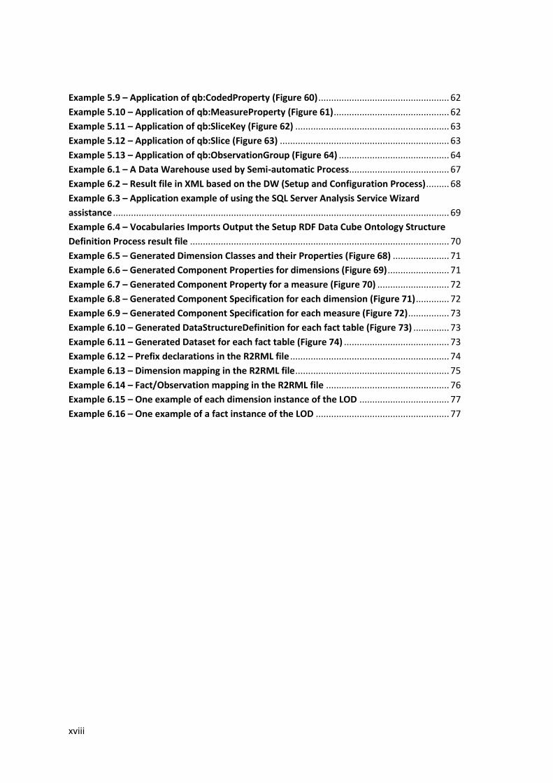
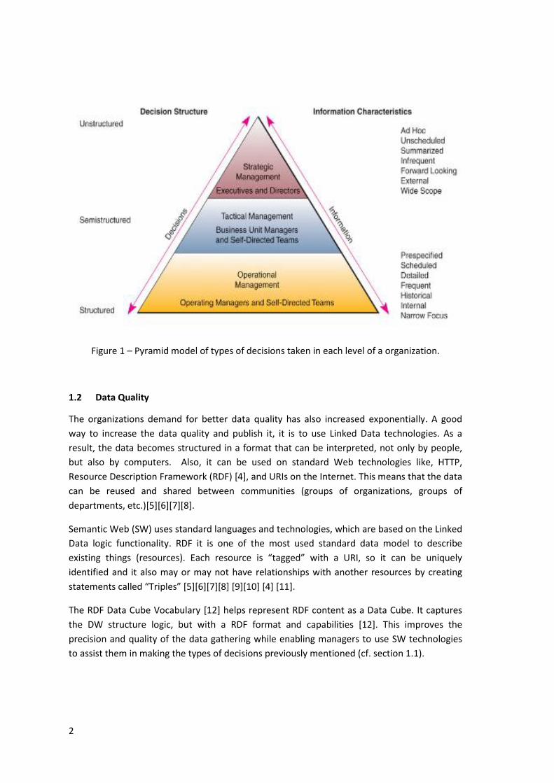
Figure 1 – Pyramid model of types of decisions taken in each level of a organization. .............. 2
Figure 2 – The interactions between OLTP and OLAP to fill Data Warehouses. .......................... 5
Figure 3 – Logical representation of a Table or View in a RDB. ................................................... 7
Figure 4 – Diagram of the most common types of tables representing a census organization. . 9
Figure 5 – Star Schema based of Figure 4. ................................................................................... 9
Figure 6 – An example of a Snowflake schema. ......................................................................... 10
Figure 7 – A example of a Galaxy schema. ................................................................................. 10
Figure 8 – Representation of the Dimensional Cube based on some tables of Figure 4. .......... 11
Figure 9 – Diagram of Slicing a Dimensional Cube. .................................................................... 12
Figure 10 – Diagram of Dicing a Dimensional Cube . ................................................................. 12
Figure 11 – Diagram of Drill-down and Roll-up a dataset. ......................................................... 13
Figure 12 – Diagram of aggregating a dataset. .......................................................................... 14
Figure 13 – Logical View of Pivot Tables. ................................................................................... 15
Figure 14 – Generic DW Architecture. ....................................................................................... 17
Figure 15 – Diagram of Kimble Architecture with its data flow. ................................................ 17
Figure 16 – Diagram of the CIF Architecture applied to an enterprise bioinformatics
information system. ................................................................................................................... 19
Figure 17 – CIF VS BUS. .............................................................................................................. 20
Figure 18 – Partial image of the LOD cloud diagram from 2011-09-19. .................................... 26
Figure 19 – RDF/XML and RDF graph describing person. .......................................................... 28
Figure 20 – OWL main sublanguages hierarchy. ........................................................................ 29
Figure 21 – Example of an OWL Lite Relationship Diagram. ...................................................... 29
Figure 22 – Example of an OWL DL Relationship Classes and Individuals with restrictions. ..... 30
Figure 23 – Example of an OWL Full Relationship Classes and Individuals with no restrictions.
.................................................................................................................................................... 30
Figure 24 – OWL profiles and sublanguages positions and hierarchy. ...................................... 31
Figure 25 – RDB to RDF in general. ............................................................................................ 34
Figure 26 – Example of a RDB Tables. ........................................................................................ 34
Figure 27 – Direct Mapping part 2a. .......................................................................................... 35
Figure 28 – Direct Mapping part 2b. .......................................................................................... 35
Figure 29 – Direct Mapping part 2c. .......................................................................................... 36
Figure 30 – Direct Mapping part 3a. .......................................................................................... 36
Figure 31 – Direct Mapping part 3b. .......................................................................................... 36
Figure 32 – Direct Mapping part 3c. .......................................................................................... 37
Figure 33 – An overview of R2RML Logic Model........................................................................ 37
Figure 34 – Result data graph from the R2RML in Table 11. ..................................................... 39
Figure 35 – Result data graph from the R2RML in Table 12. ..................................................... 40
Figure 36 – Result data graph from the R2RML in Table 13. ..................................................... 41
Figure 37 – A one-to-one Table Mapping Pattern. .................................................................... 45
Figure 38 – A one-to-many Table Mapping Pattern. ................................................................. 45
xiv
Figure 39 – A many-to-one Table Mapping Pattern. .................................................................. 46
Figure 40 – A many-to-many Table Mapping Pattern. ............................................................... 46
Figure 41 – A one-to-one Attribute Mapping Pattern. ............................................................... 47
Figure 42 – A one-to-many Attribute Mapping Pattern. ............................................................ 47
Figure 43 – A many-to-one Attribute Mapping Pattern. ............................................................ 48
Figure 44 – A many-to-many Attribute Mapping Pattern. ......................................................... 48
Figure 45 – A Concatenate Attribute Mapping Pattern. ............................................................ 49
Figure 46 – A Foreign Key between two Tables Mapping Pattern. ............................................ 49
Figure 47 – A Foreign Key between two or more Tables Mapping Pattern. .............................. 50
Figure 48 – Many to Many Tables Joining Mapping Pattern...................................................... 51
Figure 49 – A Translate Value Mapping Pattern. ....................................................................... 51
Figure 50 – A Translate values between Tables Mapping Pattern. ............................................ 52
Figure 51 – Diagram with the RDF Data Cube Vocabulary. ........................................................ 56
Figure 52 – Pivot Table of Life Expectancy based on Figure 8. .................................................. 58
Figure 53 – Example of a Dataset based on Figure 52. .............................................................. 59
Figure 54 – Example of a DataStructureDefinition based on Figure 52. .................................... 60
Figure 55 – Example of Component Specification for dimensions based on Figure 52. ............ 60
Figure 56 – Example of Component Specification for measures based on Figure 52. ............... 61
Figure 57 – Example of a DimensionProperty based on Figure 52. ........................................... 61
Figure 58 – Example of a MeasureProperty based on Figure 52. .............................................. 61
Figure 59 – Example of an AttributeProperty based on Figure 52. ............................................ 62
Figure 60 – Example of a CodedProperty based on Figure 52. .................................................. 62
Figure 61 – Example of an Observation based on Figure 52. ..................................................... 62
Figure 62 – Example of a SliceKey based on Figure 52. .............................................................. 63
Figure 63 – Example of a Slice based on Figure 52. ................................................................... 63
Figure 64 – Example of an ObservationGroup based on Figure 52. ........................................... 64
Figure 65 – The semi-automatic process diagram. .................................................................... 66
Figure 66- Data Warehouse example from SQLServer 2012. ..................................................... 67
Figure 67- Figure 66 Tables identification by SQL Server Analysis Service Wizard. ................... 69
Figure 68 – Declaration of Dimension Class and their Properties of each Dimension Table. .... 71
Figure 69 – Declaration of ComponentProperty of each Dimension Table. .............................. 71
Figure 70 – Declaration of Component Property of each measure column in a Fact Table. ..... 72
Figure 71 – Declaration of Component Specification for each dimension. ............................... 72
Figure 72 – Declaration of Component Specification the measure. .......................................... 73
Figure 73 – Graph for the DataStructureDefinition generated. ................................................. 73
Figure 74 – Graph for the Dataset generated. ........................................................................... 73
Figure 75 – One example of each dimension instance. ............................................................. 77
Figure 76 – One example of a fact record instance.................................................................... 77
Figure 77 - Semi-Process Result Ontology 3 Layers. .................................................................. 78
Figure 78 – Data Flow that passes through Bus DW Architecture. ............................................ 79
Figure 79 – Data Flow that passes through CIF DW Architecture. ............................................. 79
xv
List of Tables
Table 1 – Pros and Cons of DW relative to RDB ........................................................................... 6
Table 2 – RDB VS DW ................................................................................................................... 7
Table 3 – Most common types of tables ...................................................................................... 8
Table 4 – Dimensional Model Schemas Characteristics ............................................................. 11
Table 5 – Pros and Cons of DW BUS Architecture ..................................................................... 18
Table 6 – Pros and Cons of Corporate Information Factory Architecture ................................. 20
Table 7 – DW BUS VS DW CIF ..................................................................................................... 21
Table 8 – Rating system categories ............................................................................................ 24
Table 9 – LOD Datasets .............................................................................................................. 25
Table 10 – SPARQL query outputs of Study1 ............................................................................. 31
Table 11 – Example of R2RML Mapping without SQL from the tables on Figure 26 ................. 38
Table 12 – Example of R2RML Mapping with SQL of the tables on Figure 26 ........................... 39
Table 13 – Example of R2RML Mapping to obtain the average life expectancy........................ 41
Table 14 – Comparison Attributes ............................................................................................. 43
Table 15 – Comparison RDB2RDF Mapping Languages and technologies using the Table 14
characteristics ............................................................................................................................ 44
Table 16 – Relational Database knowledge Levels that use Algorithms .................................... 53
Table 17 – RDB to RDF patterns VS Virtuoso/D2RQ/Triplify/ontop .......................................... 54
Table 18-Direct Mapping Code results from section 4.1.1 ........................................................ 91
Table 19-Example of R2RML Mapping result without SQL from Table 11 ................................. 92
Table 20- Example of R2RML Mapping result with SQL from Table 12 ..................................... 92
Table 21 – Some query applications based on the example in Figure 52 .................................. 93

xvi
xvii
List of Examples
Example 2.1 – Star Schema ......................................................................................................... 9
Example 2.2 – Simple Snowflake Schema ................................................................................ 10
Example 2.3 – Galaxy/Fact Constellation Schema ................................................................... 10
Example 2.4 – Simple Dimensional Cube .................................................................................. 11
Example 2.5 – Slicing operation of a Dimensional Cube .......................................................... 12
Example 2.6 – Dicing operation of a Dimensional Cube .......................................................... 12
Example 2.7 – Roll-up operation of a Dimensional Cube ......................................................... 13
Example 2.9 – Aggregation operation of a Dimensional Cube ................................................ 14
Example 2.10 – Pivot Table creation from a Dimensional Cube .............................................. 14
Example 3.1 – Ontology Using FOAF Ontology ........................................................................ 28
Example 3.2 – OWL Lite Property Cardinality constraint with value 1 .................................... 29
Example 3.3 – OWL DL with border between Classes and Individuals constraint .................. 30
Example 3.4 – OWL Full with no border between Classes and Individuals ............................. 30
Example 3.5 – A simple SPARQL query with its result ............................................................. 31
Example 4.1 – A simple Direct Mapping ................................................................................... 35
Example 4.2 – R2RML without SQL Instructions applied ......................................................... 38
Example 4.3 – R2RML with SQL Instructions applied ............................................................... 39
Example 4.4 – Case of R2RML mapping using SQL Operator “AND” and Function “AVG()” .. 41
Example 4.5 – One-to-one(1:1) Table Mapping (Figure 37) ..................................................... 45
Example 4.6 – One-to-many(1:*) Table Mapping (Figure 38) .................................................. 45
Example 4.7 – Many-to-one (*:1) Table Mapping (Figure 39) ................................................. 46
Example 4.8 – Many-to-many (*:*) Table Mapping (Figure 40) .............................................. 46
Example 4.9 – One-to-one(1:1) Attribute Mapping (Figure 41) ............................................... 47
Example 4.10 – One-to-many(1:*) Attribute Mapping (Figure 42) .......................................... 47
Example 4.11 – Many-to-one(*:1) Attribute Mapping (Figure 43) .......................................... 48
Example 4.12 – Many-to-many(*:*) Attribute Mapping (Figure 44) ....................................... 48
Example 4.13 – Concatenate Attribute Mapping (Figure 45) .................................................. 49
Example 4.14 – Foreign Key between two tables Join Mapping (Figure 46) ........................... 49
Example 4.15 – Foreign Key between two or more tables Join Mapping (Figure 47) ............ 50
Example 4.16 – Many-to-many Tables Join Mapping (Figure 48) ............................................ 51
Example 4.17 – Translate a value Mapping(Figure 49) ............................................................ 51
Example 4.18 – Translate values between tables Mapping (Figure 50) .................................. 52
Example 5.1 – Application of the RDF Data Cube Vocabulary in scenario .............................. 58
Example 5.2 – Application of qb:DataSet (Figure 53) .............................................................. 59
Example 5.3 – Application of qb:DataStructureDefinition (Figure 54) .................................... 60
Example 5.4 – Application of qb:ComponentSpecification for Dimensions(Figure 55) .......... 60
Example 5.5 – Application of qb:ComponentSpecification for Measures(Figure 56) ............. 61
Example 5.6 – Application of qb:DimensionProperty (Figure 57) ........................................... 61
Example 5.7 – Application of qb:MeasureProperty (Figure 58) .............................................. 61
Example 5.8 – Application of qb:AttributeProperty (Figure 59) .............................................. 62
xviii
Example 5.9 – Application of qb:CodedProperty (Figure 60) ................................................... 62
Example 5.10 – Application of qb:MeasureProperty (Figure 61) ............................................. 62
Example 5.11 – Application of qb:SliceKey (Figure 62) ............................................................ 63
Example 5.12 – Application of qb:Slice (Figure 63) .................................................................. 63
Example 5.13 – Application of qb:ObservationGroup (Figure 64) ........................................... 64
Example 6.1 – A Data Warehouse used by Semi-automatic Process ....................................... 67
Example 6.2 – Result file in XML based on the DW (Setup and Configuration Process) ......... 68
Example 6.3 – Application example of using the SQL Server Analysis Service Wizard
assistance ................................................................................................................................... 69
Example 6.4 – Vocabularies Imports Output the Setup RDF Data Cube Ontology Structure
Definition Process result file ..................................................................................................... 70
Example 6.5 – Generated Dimension Classes and their Properties (Figure 68) ...................... 71
Example 6.6 – Generated Component Properties for dimensions (Figure 69) ........................ 71
Example 6.7 – Generated Component Property for a measure (Figure 70) ............................ 72
Example 6.8 – Generated Component Specification for each dimension (Figure 71) ............. 72
Example 6.9 – Generated Component Specification for each measure (Figure 72) ................ 73
Example 6.10 – Generated DataStructureDefinition for each fact table (Figure 73) .............. 73
Example 6.11 – Generated Dataset for each fact table (Figure 74) ......................................... 73
Example 6.12 – Prefix declarations in the R2RML file .............................................................. 74
Example 6.13 – Dimension mapping in the R2RML file ............................................................ 75
Example 6.14 – Fact/Observation mapping in the R2RML file ................................................ 76
Example 6.15 – One example of each dimension instance of the LOD ................................... 77
Example 6.16 – One example of a fact instance of the LOD .................................................... 77
xix
List of Abbreviations
BI Business Intelligence
CIF Corporate Information Factory
DCMI Dublin Core Metadata Initiative
DM Direct Mapping
DSS Decision Support Systems
DW Data Warehouse
ETL Extraction, Transformation and Load Process
ER Entity Relationship
FOAF Friend of a Friend
GLD Government Linked Data
HTTP Hypertext Transfer Protocol
LOD Linked Open Data
LOV Linked Open Vocabularies
N3 Notation3
ODS Operational Data Store
OLAP On-line Analytical Processing
OLTP On-line Transactional Processing
OWL Web Ontology Language
RDB Relational Database
R2RML RDB to RDF Mapping Language
RDF Resource Description Framework
SKOS Simple knowledge Organization System
SPARQL Simple Protocol and RDF Query Language
SQL Structured Query Language
xx
SW Semantic Web
TCP/IP Transmission Control Protocol / Internet Protocol
URI Uniform Resource Identifier
W3C World Wide Web Consortium
XML eXtensible Markup Language

1
1 Introduction
1.1 Organizations and data gathering
The organizations managers of today have urgent demands to gather great volumes of
data/information for the purpose of using them in their decisions. The types of decisions that
those managers can make affecting their organization are (cf. Figure 1) [1][2]:
Operational, in terms of running routine management operations (Structured);
Tactical, in terms of remain compatible in the markets or in its business field (Semi-
structured);
Strategic, in terms future actions or expansion of the organization (Unstructured).
Using Decision Support Systems (DSS) or Business Intelligence (BI) is the best solution for
Strategic and Tactical decisions because they do not have a fix procedure structure[1] [2]. DSS
is a interactive and malleable computer-base system that is capable of solving unstructured
and semi-structured decision problems, by adapting to each situation [1][2][3]. BI is an
evolved strand of DSS dedicated to transform great amounts of structured and unstructured
raw data into meaningful information that can be used to do [1] [2][3]:
Data analyses;
Reports;
Data and text mining;
On-line Analytical Processing (OLAP);
Etc.
Data Warehouses (DW) are OLAP databases that DSS and BI use for [1] [2]:
Storing the gathered data in a dimensional model format;
Executing data analyses;
Creating reports.
2
Figure 1 – Pyramid model of types of decisions taken in each level of a organization.
1.2 Data Quality
The organizations demand for better data quality has also increased exponentially. A good
way to increase the data quality and publish it, it is to use Linked Data technologies. As a
result, the data becomes structured in a format that can be interpreted, not only by people,
but also by computers. Also, it can be used on standard Web technologies like, HTTP,
Resource Description Framework (RDF) [4], and URIs on the Internet. This means that the data
can be reused and shared between communities (groups of organizations, groups of
departments, etc.)[5][6][7][8].
Semantic Web (SW) uses standard languages and technologies, which are based on the Linked
Data logic functionality. RDF it is one of the most used standard data model to describe
existing things (resources). Each resource is “tagged” with a URI, so it can be uniquely
identified and it also may or may not have relationships with another resources by creating
statements called “Triples” [5][6][7][8] [9][10] [4] [11].
The RDF Data Cube Vocabulary [12] helps represent RDF content as a Data Cube. It captures
the DW structure logic, but with a RDF format and capabilities [12]. This improves the
precision and quality of the data gathering while enabling managers to use SW technologies
to assist them in making the types of decisions previously mentioned (cf. section 1.1).
3
1.3 Main goal
Most of the existing data on the Internet is not stored according to the Linked Data format
principles. In fact, most of the data is stored in Relational Databases and it is accessible
through a SQL statement. Those databases represent a big percentage of raw data sources
that undergo a process that extracts, transforms and loads (ETL) its result into Data
Warehouses for the purpose mention on section 1.1.
Has mentioned in section 1.2, RDF Data Cubes are superior to Data Warehouses because:
It enables the use of SW technology;
It promotes/has better quality data;
It can be seen/manipulated (i) as a relational model and (ii) as dimensional model at
the same time.
This raises two sets of problems:
1. Data Warehouses are easy to use and have great amounts of data, but no direct
compatibility with SW technologies due to the fact it doesn’t use any of the Linked
Data principles;
2. RDF Data Cubes are more complex to use compared to DW, but it can be used by SW
technologies.
So, the solution is the creation of a data repository that uses Linked Data technology and has
the Data Warehouse capabilities via the RDF Data Cube Vocabulary use.
Considering this, the work described in this document is focused on the following research
question: “How do I convert Data Warehouse data into a RDF Data Cube in a simple and easy
fashion?”
In order to provide a (possible) answer to that question, the goal of this work is to propose a
semi-automatic process that creates a RDF Data Cube from a given Data Warehouse and
keeps its data content updated while enable it to be presented (i) in a relational and (ii) in a
dimensional format.
1.4 The Thesis Content
This thesis contains seven chapters:
The first and current chapter introduces the document context and main goal.
The second chapter presents an overview of Data Warehouses that are the sources of the
semi-automatic process that will create the data repository.
The third chapter presents an analysis of Linked Data, namely its concept, principles and
languages that can be used to express it. One of those languages (RDF or OWL) in combination
4
with a serialization method (e.g. XML, N-Triples, etc) is the result format of the data repository
that the semi-automated process can create;
The forth chapter presents the survey of RDB to RDF Mapping languages and technologies, in
which R2RML is used by the semi-automatic process to create mapping between a Data
Warehouse (cf. Chapter 2) and the data repository (cf. Chapter 3 and Chapter 5).
The fifth chapter presents the RDF Data Cube Vocabulary, that is going to be used in classify
the data repository created by the semi-automatic process, as a Data Cube.
The sixth chapter presents and describes semi-automatic process proposed with a running
example that evolves along side with every implemented step.
The final chapter 7 presents the conclusions gain from this work and some possible limitations.
Also, it contains some suggestions of possible future work that can be added to the semi-
automatic process.
5
2 Data Warehouse Overview
In this chapter, it is presented an overview of the data source used by the semi-automated
process.
2.1 What is a Data Warehouses?
As it is mention in section 1.1, managers make types of decisions that affect their organization.
Therefore, to address Operational decision it can be used Operational Systems or On-Line
Transactional Process (OLTP) systems because they are design to do routine transaction
processing of data into databases. OLTP Database or Relational Databases (RDB) has detailed
and current data that is applied in Operational Data Stores (ODS) or as source for OLAP
Databases [1][13][14][15][16][17]. And to address Strategic and Tactical decisions it can be
used DSS or On-Line Analytical Process (OLAP) systems because they are used to do analysis
on data that is stored in Data Warehouses (DW). OLAP Databases have aggregated and
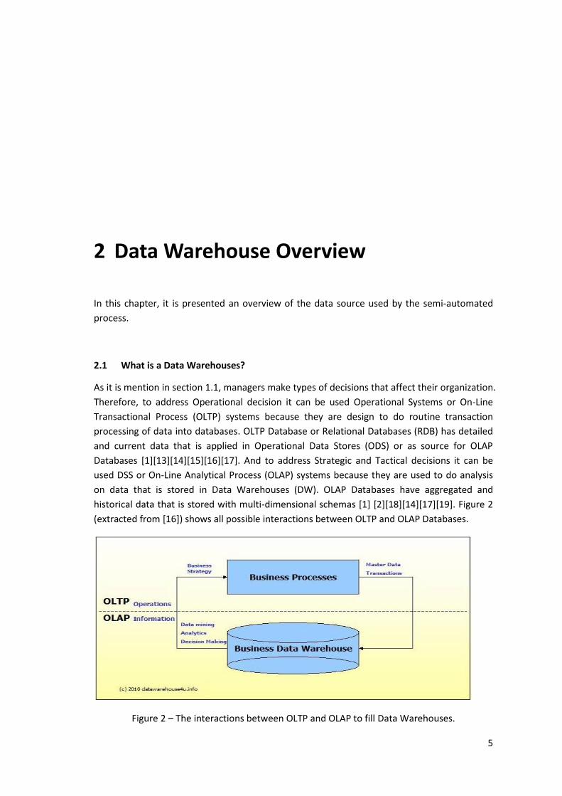
historical data that is stored with multi-dimensional schemas [1] [2][18][14][17][19]. Figure 2
(extracted from [16]) shows all possible interactions between OLTP and OLAP Databases.
Figure 2 – The interactions between OLTP and OLAP to fill Data Warehouses.
6
A DW is a database that uses the Dimensional model [20][21] to store data as a central
repository, where all the data comes from multiple sources, like RDB, text files, Excel files, etc.
A DW is used for analysis and reports since it is design to give a fast query response. The data
in the Dimensional model is represented in a logical structure that uses the concept of a cube,
called Dimensional Cube. A Cube is a multi-dimensional structure that contains [1][17][20]
[21][22][23]:
Facts - are things that happens in a context that implies a transaction or an event, like
a sale in a store, restock of inventory, etc. Therefore, a “non-facts” (things that didn’t
happened) are not save, making the cube hollow like a “Swiss cheese”;
Dimensions – are characteristics that help identify or search a fact, like dates, places,
products, etc.
2.2 RDB VS DW
According to references [24], [25] and [26], a DW “is not a product, or hardware, or software”.
Instead, it is a system architecture that saves “events”. Those “events” can be sales
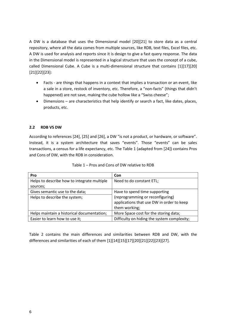
transactions, a census for a life expectancy, etc. The Table 1 (adapted from [24]) contains Pros
and Cons of DW, with the RDB in consideration.
Table 1 – Pros and Cons of DW relative to RDB
Pro Con
Helps to describe how to integrate multiple sources;
Need to do constant ETL;
Gives semantic use to the data; Have to spend time supporting (reprogramming or reconfiguring) applications that use DW in order to keep them working;
Helps to describe the system;
Helps maintain a historical documentation; More Space cost for the storing data;
Easier to learn how to use it; Difficulty on hiding the system complexity;
Table 2 contains the main differences and similarities between RDB and DW, with the
differences and similarities of each of them [1][14][15][17][20][21][22][23][27].
7
Table 2 – RDB VS DW
RDB DW
Process OLTP OLAP
Data Model Entity-Relational Model Dimensional Model
Schemas Normalized (Typically at the 3º form).
Star, Snowflake, Galaxy, etc.
Actualization Instantaneous refresh. Periodically refresh
Data Save Update, old information loss. Historical, no information loss.
Data Storage Optimized Space, no data repetition.
More Space than RDB because of data redundancy.
Usage Normally, it is constrained to one application. For quick real-time data transactions.
More than one application. For data analysis, reports and decision-making.
Similarities They use SQL to query the data.
They store and manage data, using tables and views that have the structure seen in Figure 3.
They have data types.
They use the same relation between table logic (Example: Dimensional Model uses ER model to relate dimensions tables to a fact table).
2.3 Dimensional Cube
2.3.1 Types of Tables in Dimensional Cube
A RDB is a database that uses the Entity-Relational (ER) Model structure to store information
about the data and relationships they have. The ER model is a data model that describes how
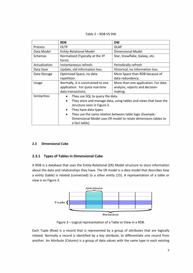
a entity (table) is related (connected) to a other entity [15]. A representation of a table or
view is on Figure 3.
Figure 3 – Logical representation of a Table or View in a RDB.
Each Tuple (Row) is a record that is represented by a group of attributes that are logically
related. Normally a record is identified by a key attribute, to differentiate one record from
another. An Attribute (Column) is a group of data values with the same type in each existing
8
record. A Relation is a formal data structure that guaranties that all the Tuples, in a Table,
have the same number and types of Attributes with the same designation[15].
As mention in section 2.1, Dimensional Cube relies on the Dimensional Model which instead
relies on the basic functionalities of ER Models, like tables and relationships between them.
Therefore, the structure of a Dimensional Cube is basically a group of tables that are
connected between them and have a schema (e.g. star schema, snowflake schema, etc)
applied to them. The two main types of table are the Dimensional Tables and Fact Tables. The
Fact Table’s columns, besides the identification key column, are the measures with details of a
fact (row). The Dimensional Table’s columns, besides the identification key column, are
attributes that are used in queries that provides a certain semantic level detail to retrieve a
fact or a collection of facts from the Fact Table[1][20][21][28]. Table 3 contains some of the
most used types of tables when conceiving a Dimensional Cube[1][20][21][28].
Table 3 – Most common types of tables
Name Description
Fact Table
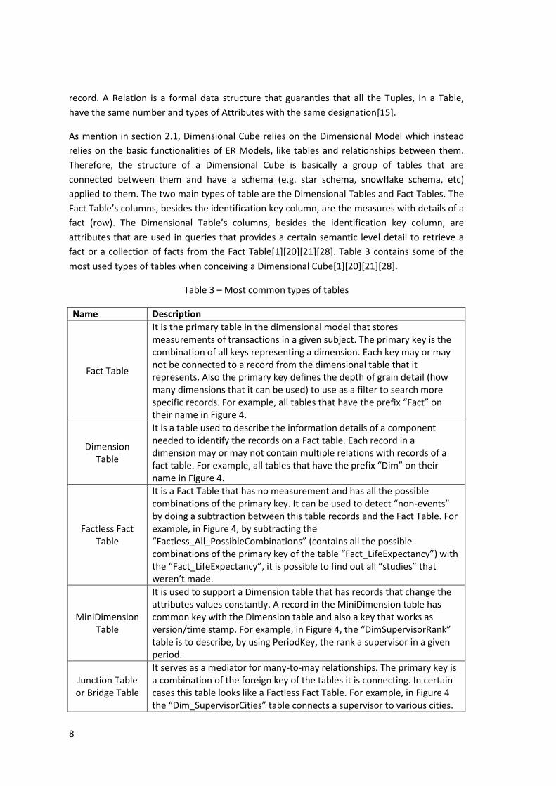
It is the primary table in the dimensional model that stores measurements of transactions in a given subject. The primary key is the combination of all keys representing a dimension. Each key may or may not be connected to a record from the dimensional table that it represents. Also the primary key defines the depth of grain detail (how many dimensions that it can be used) to use as a filter to search more specific records. For example, all tables that have the prefix “Fact” on their name in Figure 4.
Dimension Table
It is a table used to describe the information details of a component needed to identify the records on a Fact table. Each record in a dimension may or may not contain multiple relations with records of a fact table. For example, all tables that have the prefix “Dim” on their name in Figure 4.
Factless Fact Table
It is a Fact Table that has no measurement and has all the possible combinations of the primary key. It can be used to detect “non-events” by doing a subtraction between this table records and the Fact Table. For example, in Figure 4, by subtracting the “Factless_All_PossibleCombinations” (contains all the possible combinations of the primary key of the table “Fact_LifeExpectancy”) with the “Fact_LifeExpectancy”, it is possible to find out all “studies” that weren’t made.
MiniDimension Table
It is used to support a Dimension table that has records that change the attributes values constantly. A record in the MiniDimension table has common key with the Dimension table and also a key that works as version/time stamp. For example, in Figure 4, the “DimSupervisorRank” table is to describe, by using PeriodKey, the rank a supervisor in a given period.
Junction Table or Bridge Table
It serves as a mediator for many-to-may relationships. The primary key is a combination of the foreign key of the tables it is connecting. In certain cases this table looks like a Factless Fact Table. For example, in Figure 4 the “Dim_SupervisorCities” table connects a supervisor to various cities.
9
Figure 4 – Diagram of the most common types of tables representing a census organization.
2.3.2 Types of Dimensional Model Schema
The Dimensional Model has structures, known as “schema”. They define how the data will be
used, stored and represented. Some of their types are [1][29][30]:
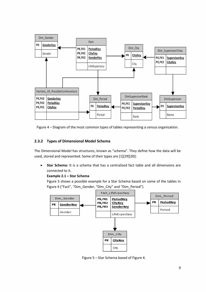
Star Schema: It is a schema that has a centralized fact table and all dimensions are
connected to it.
Example 2.1 – Star Schema
Figure 5 shows a possible example for a Star Schema based on some of the tables in
Figure 4 (“Fact”, “Dim_Gender, “Dim_City” and “Dim_Period”).
Figure 5 – Star Schema based of Figure 4.
10
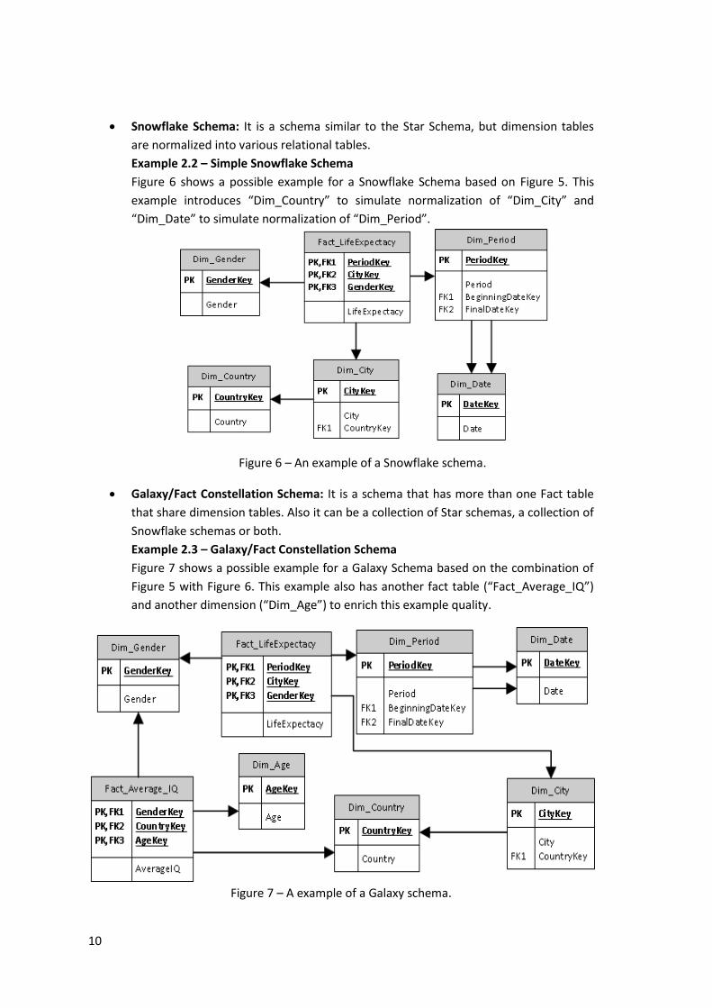
Snowflake Schema: It is a schema similar to the Star Schema, but dimension tables
are normalized into various relational tables.
Example 2.2 – Simple Snowflake Schema
Figure 6 shows a possible example for a Snowflake Schema based on Figure 5. This
example introduces “Dim_Country” to simulate normalization of “Dim_City” and
“Dim_Date” to simulate normalization of “Dim_Period”.
Figure 6 – An example of a Snowflake schema.
Galaxy/Fact Constellation Schema: It is a schema that has more than one Fact table
that share dimension tables. Also it can be a collection of Star schemas, a collection of
Snowflake schemas or both.
Example 2.3 – Galaxy/Fact Constellation Schema
Figure 7 shows a possible example for a Galaxy Schema based on the combination of
Figure 5 with Figure 6. This example also has another fact table (“Fact_Average_IQ”)
and another dimension (“Dim_Age”) to enrich this example quality.
Figure 7 – A example of a Galaxy schema.
11
A comparison of advantages and disadvantages of each schema is showed in Table
4[1][29][30].
Table 4 – Dimensional Model Schemas Characteristics
Schema Characteristics
Star Simple Queries
Fast Query response compared to Snowflake
Fast Aggregations
Easy ETL Output solution;
Cannot guaranty data integrity
Snowflake Compared to the Star Schema:
it uses less storage space
it has better data integrity
the queries are more complex The Galaxy or Fact Constellation
Reusability of existing tables on different Fact Tables
Same complexity and usability as the Star Schema, but with more Fact Tables
2.3.3 Operations on Dimensional Cubes
As said on section 1.1, a DW is commonly applied in Business Intelligence and Decision Making
Support areas because it has an improved time response from queries than the RDB
[1][17][22]. Most of this improvement comes from the accuracy of relevant data provided by
the operational capabilities that Dimensional Cubes have.
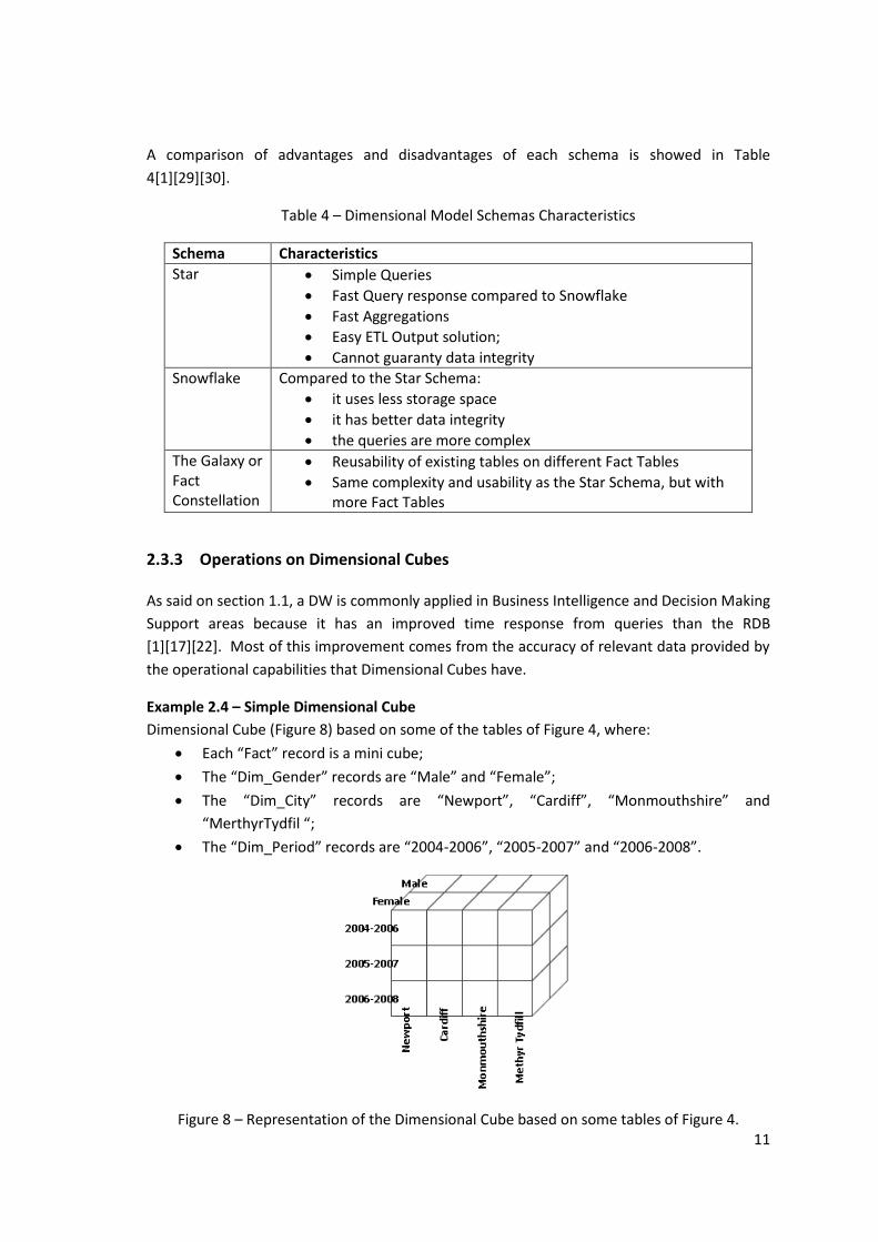
Example 2.4 – Simple Dimensional Cube
Dimensional Cube (Figure 8) based on some of the tables of Figure 4, where:
Each “Fact” record is a mini cube;
The “Dim_Gender” records are “Male” and “Female”;
The “Dim_City” records are “Newport”, “Cardiff”, “Monmouthshire” and
“MerthyrTydfil “;
The “Dim_Period” records are “2004-2006”, “2005-2007” and “2006-2008”.
Figure 8 – Representation of the Dimensional Cube based on some tables of Figure 4.
12
To better identify and explain how Dimensional Cube operations work, the dimensional cube
of Example 2.4 is used as a running example. The operations in question are [19][31]:
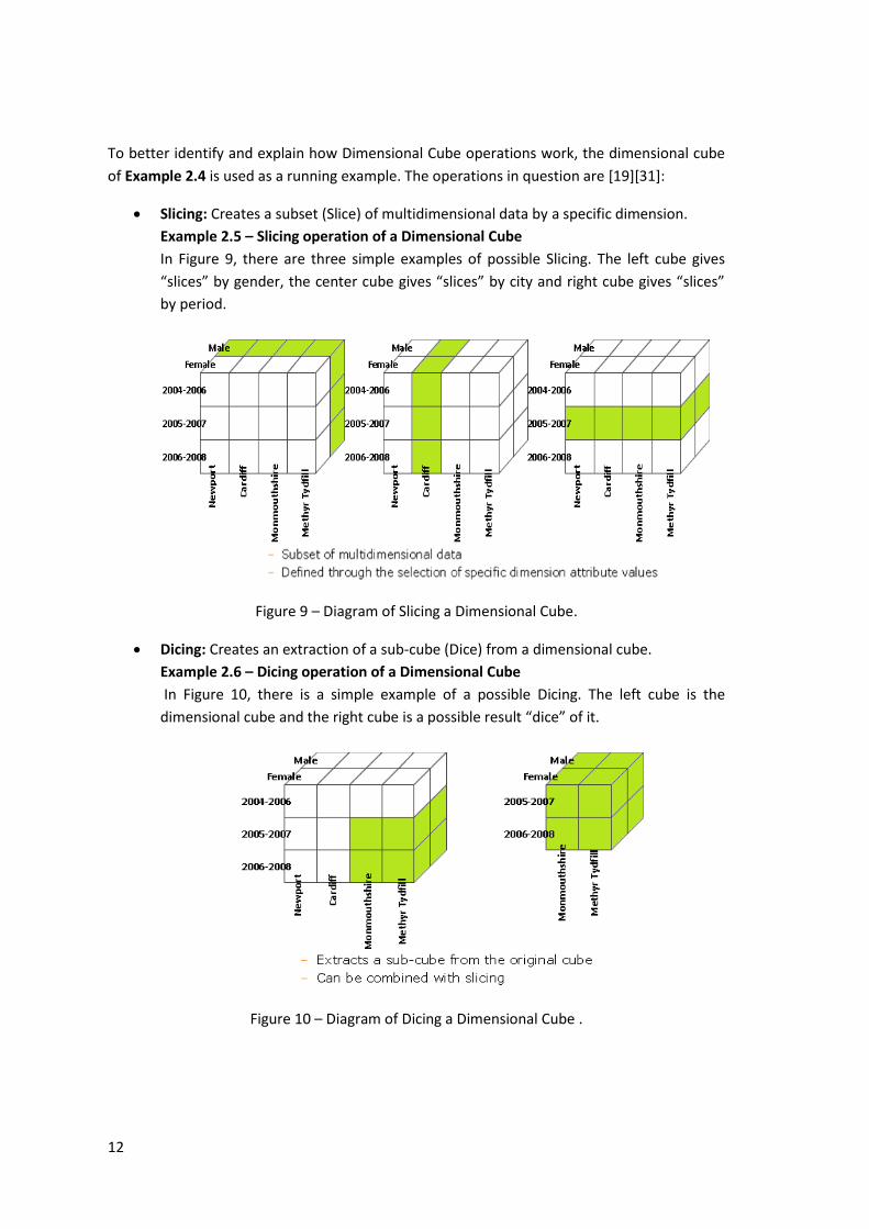
Slicing: Creates a subset (Slice) of multidimensional data by a specific dimension.
Example 2.5 – Slicing operation of a Dimensional Cube
In Figure 9, there are three simple examples of possible Slicing. The left cube gives
“slices” by gender, the center cube gives “slices” by city and right cube gives “slices”
by period.
Figure 9 – Diagram of Slicing a Dimensional Cube.
Dicing: Creates an extraction of a sub-cube (Dice) from a dimensional cube.
Example 2.6 – Dicing operation of a Dimensional Cube
In Figure 10, there is a simple example of a possible Dicing. The left cube is the
dimensional cube and the right cube is a possible result “dice” of it.
Figure 10 – Diagram of Dicing a Dimensional Cube .
13
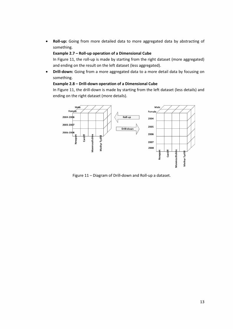
Roll-up: Going from more detailed data to more aggregated data by abstracting of
something.
Example 2.7 – Roll-up operation of a Dimensional Cube
In Figure 11, the roll-up is made by starting from the right dataset (more aggregated)
and ending on the result on the left dataset (less aggregated).
Drill-down: Going from a more aggregated data to a more detail data by focusing on
something.
Example 2.8 – Drill-down operation of a Dimensional Cube
In Figure 11, the drill-down is made by starting from the left dataset (less details) and
ending on the right dataset (more details).
Figure 11 – Diagram of Drill-down and Roll-up a dataset.
14
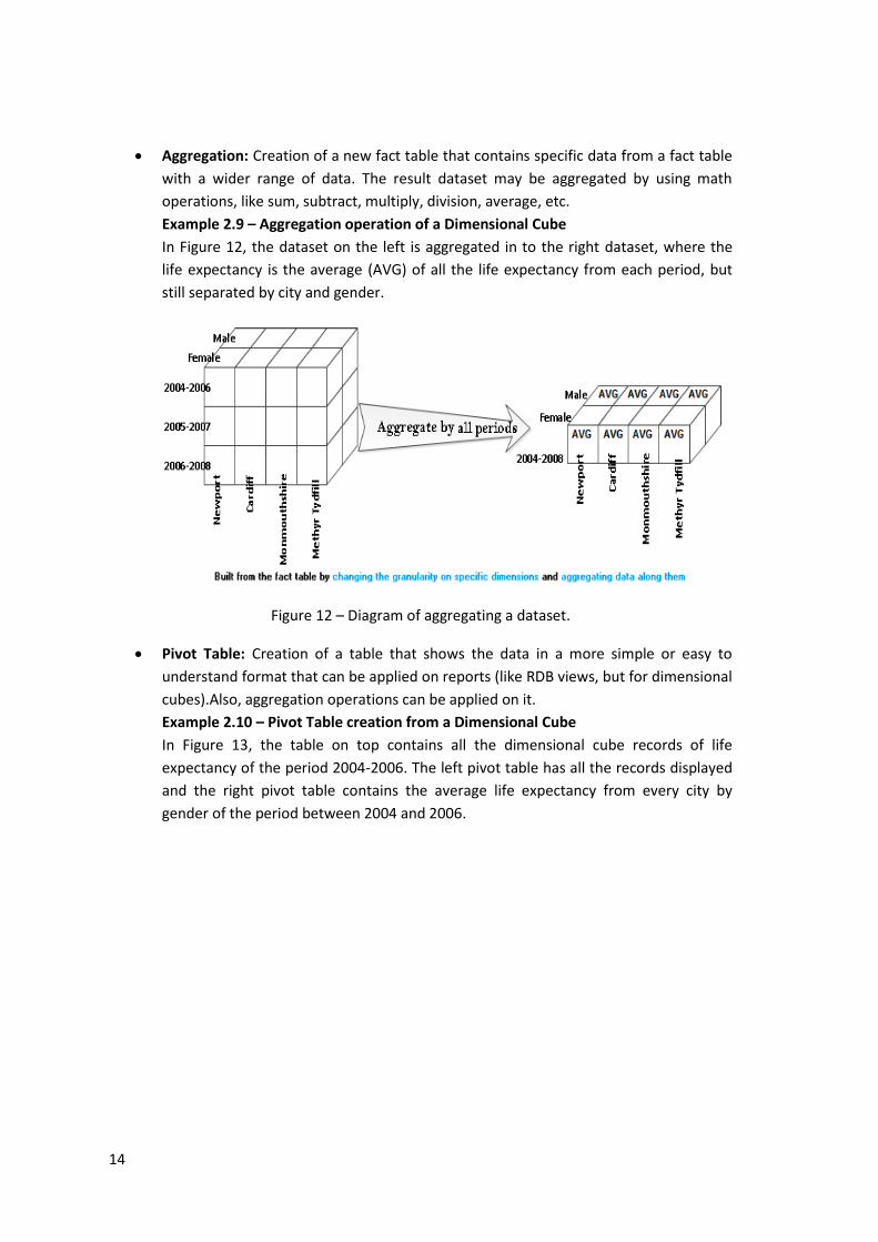
Aggregation: Creation of a new fact table that contains specific data from a fact table
with a wider range of data. The result dataset may be aggregated by using math
operations, like sum, subtract, multiply, division, average, etc.
Example 2.9 – Aggregation operation of a Dimensional Cube
In Figure 12, the dataset on the left is aggregated in to the right dataset, where the
life expectancy is the average (AVG) of all the life expectancy from each period, but
still separated by city and gender.
Figure 12 – Diagram of aggregating a dataset.
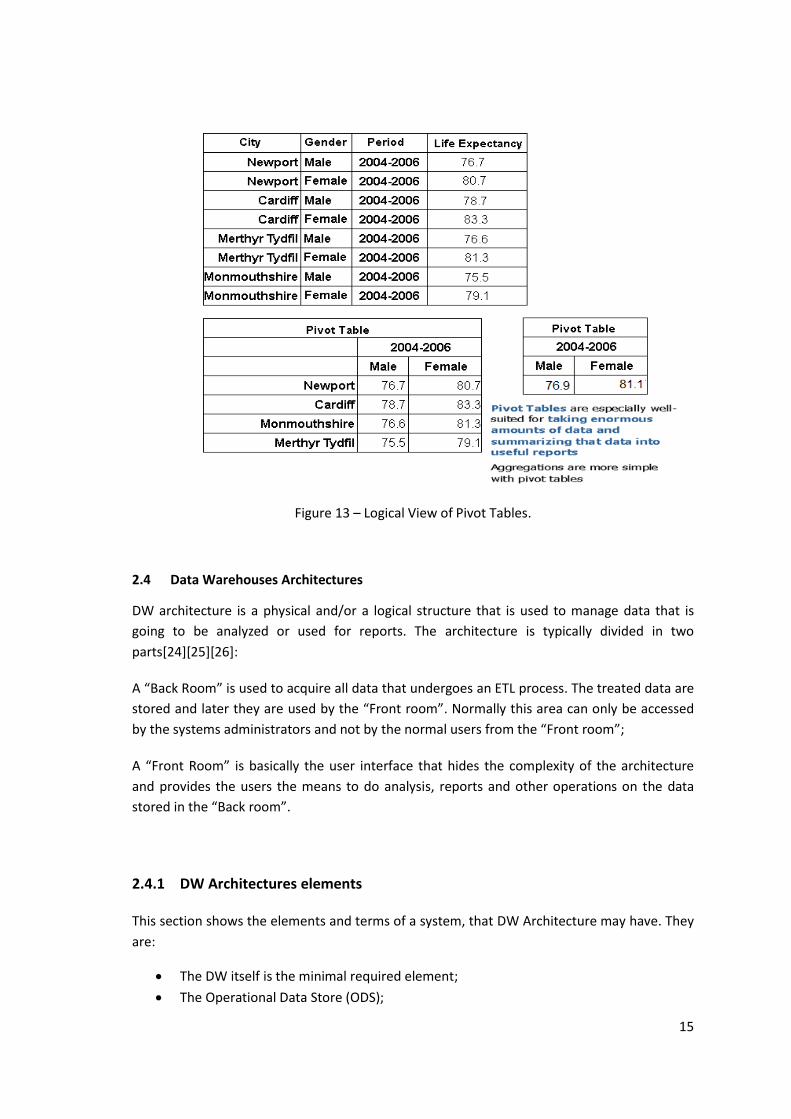
Pivot Table: Creation of a table that shows the data in a more simple or easy to
understand format that can be applied on reports (like RDB views, but for dimensional
cubes).Also, aggregation operations can be applied on it.
Example 2.10 – Pivot Table creation from a Dimensional Cube
In Figure 13, the table on top contains all the dimensional cube records of life
expectancy of the period 2004-2006. The left pivot table has all the records displayed
and the right pivot table contains the average life expectancy from every city by
gender of the period between 2004 and 2006.
15
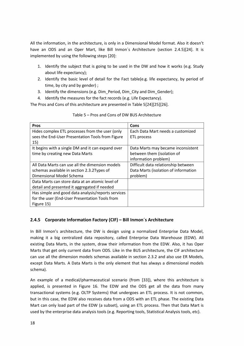
Figure 13 – Logical View of Pivot Tables.
2.4 Data Warehouses Architectures
DW architecture is a physical and/or a logical structure that is used to manage data that is
going to be analyzed or used for reports. The architecture is typically divided in two
parts[24][25][26]:
A “Back Room” is used to acquire all data that undergoes an ETL process. The treated data are
stored and later they are used by the “Front room”. Normally this area can only be accessed
by the systems administrators and not by the normal users from the “Front room”;
A “Front Room” is basically the user interface that hides the complexity of the architecture
and provides the users the means to do analysis, reports and other operations on the data
stored in the “Back room”.
2.4.1 DW Architectures elements
This section shows the elements and terms of a system, that DW Architecture may have. They
are:
The DW itself is the minimal required element;
The Operational Data Store (ODS);
16
The Data Mart;
The Oper Mart;
The ODS is a database that stores only the current data with almost real-time refresh rate.
That means it doesn’t have the capability of cross check data progressing during periods of
time, like DW has. ODS can be structured in relational model or dimensional model format,
depending of which one is more useful to present the data[24][25][26].
The Data Mart is a miniaturized Data Warehouse designed to help store and analyze data of a
specific theme. It is an autonomous element in terms of data. This means that the data can be
outdated, but on the bright side, it has optimized performance response for
queries[24][25][26].
The Oper Mart is a miniaturized Operational Data Store that has the same structure as the
Data Mart. It has, like the ODS, only real-time data, making it useful for current visualizations,
but inconsistent as time passes.
2.4.2 ETL
There is process that helps integrating data from multiple sources (e.g. RDB, documents, etc.)
to a destination database (DW or ODS) known as ETL. This process is divided in three steps
[32]:
1. Extraction – is when the process selects and retrieves the data from a source or
multiple sources. The sources can be all kinds of data, like relational databases, flat
files and non-relational databases. The more complex the source data is the more
difficult is the “Transformation” phase of the ETL process.
2. Transformation – is when all the data is formatted into a uniform logic structure,
based on some programmable instructions. It resolves errors and missing data;
3. Loading – is when the data is put into the DW.
Typically, this process is expensive and time consuming, since there is not an automated
creation process for the ETL mappings [32].
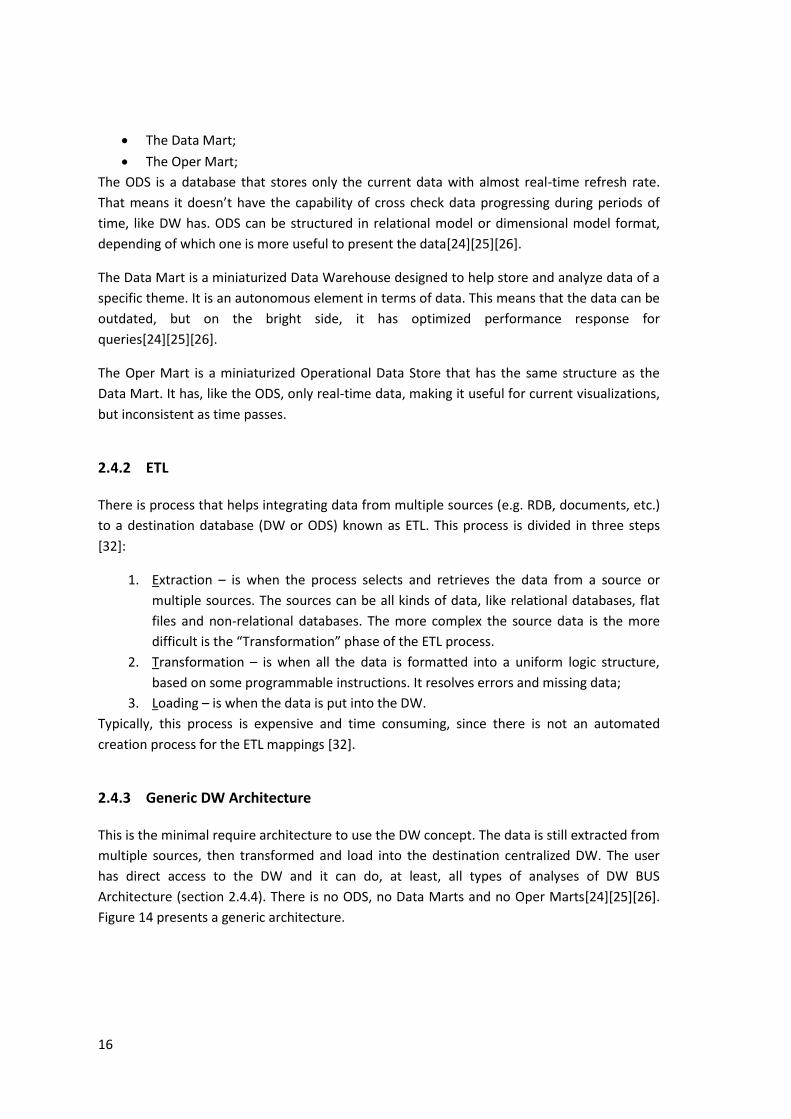
2.4.3 Generic DW Architecture
This is the minimal require architecture to use the DW concept. The data is still extracted from
multiple sources, then transformed and load into the destination centralized DW. The user
has direct access to the DW and it can do, at least, all types of analyses of DW BUS
Architecture (section 2.4.4). There is no ODS, no Data Marts and no Oper Marts[24][25][26].
Figure 14 presents a generic architecture.
17
Figure 14 – Generic DW Architecture.
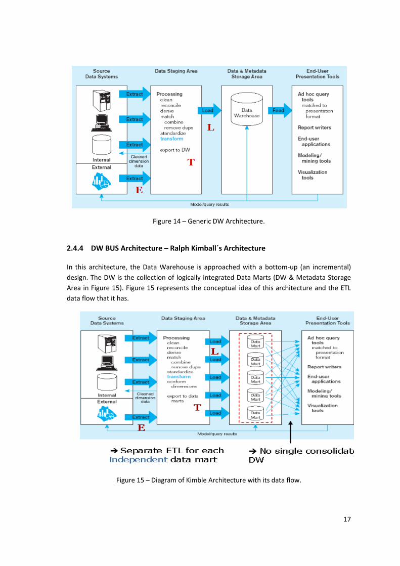
2.4.4 DW BUS Architecture – Ralph Kimball´s Architecture
In this architecture, the Data Warehouse is approached with a bottom-up (an incremental)
design. The DW is the collection of logically integrated Data Marts (DW & Metadata Storage
Area in Figure 15). Figure 15 represents the conceptual idea of this architecture and the ETL
data flow that it has.
Figure 15 – Diagram of Kimble Architecture with its data flow.
18
All the information, in the architecture, is only in a Dimensional Model format. Also it doesn’t
have an ODS and an Oper Mart, like Bill Inmon´s Architecture (section 2.4.5)[24]. It is
implemented by using the following steps [20]:
1. Identify the subject that is going to be used in the DW and how it works (e.g. Study
about life expectancy);
2. Identify the basic level of detail for the Fact table(e.g. life expectancy, by period of
time, by city and by gender) ;
3. Identify the dimensions (e.g. Dim_Period, Dim_City and Dim_Gender);
4. Identify the measures for the fact records (e.g. Life Expectancy).
The Pros and Cons of this architecture are presented in Table 5[24][25][26].
Table 5 – Pros and Cons of DW BUS Architecture
Pros Cons
Hides complex ETL processes from the user (only sees the End-User Presentation Tools from Figure 15)
Each Data Mart needs a customized ETL process
It begins with a single DM and it can expand over time by creating new Data Marts
Data Marts may became inconsistent between them (isolation of information problem)
All Data Marts can use all the dimension models schemas available in section 2.3.2Types of Dimensional Model Schema
Difficult data relationship between Data Marts (isolation of information problem)
Data Marts can store data at an atomic level of detail and presented it aggregated if needed
Has simple and good data analysis/reports services for the user (End-User Presentation Tools from Figure 15)
2.4.5 Corporate Information Factory (CIF) – Bill Inmon´s Architecture
In Bill Inmon’s architecture, the DW is design using a normalized Enterprise Data Model,
making it a big centralized data repository, called Enterprise Data Warehouse (EDW). All
existing Data Marts, in the system, draw their information from the EDW. Also, it has Oper
Marts that get only current data from ODS. Like in the BUS architecture, the CIF architecture
can use all the dimension models schemas available in section 2.3.2 and also use ER Models,
except Data Marts. A Data Marts is the only element that has always a dimensional models
schema).
An example of a medical/pharmaceutical scenario (from [33]), where this architecture is
applied, is presented in Figure 16. The EDW and the ODS get all the data from many
transactional systems (e.g. OLTP Systems) that undergoes an ETL process. It is not common,
but in this case, the EDW also receives data from a ODS with an ETL phase. The existing Data
Mart can only load part of the EDW (a subset), using an ETL process. Then that Data Mart is
used by the enterprise data analysis tools (e.g. Reporting tools, Statistical Analysis tools, etc).
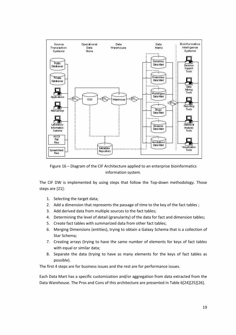
19
Figure 16 – Diagram of the CIF Architecture applied to an enterprise bioinformatics
information system.
The CIF DW is implemented by using steps that follow the Top-down methodology. Those
steps are [21]:
1. Selecting the target data;
2. Add a dimension that represents the passage of time to the key of the fact tables ;
3. Add derived data from multiple sources to the fact tables;
4. Determining the level of detail (granularity) of the data for fact and dimension tables;
5. Create fact tables with summarized data from other fact tables;
6. Merging Dimensions (entities), trying to obtain a Galaxy Schema that is a collection of
Star Schema;
7. Creating arrays (trying to have the same number of elements for keys of fact tables
with equal or similar data;
8. Separate the data (trying to have as many elements for the keys of fact tables as
possible).
The first 4 steps are for business issues and the rest are for performance issues.
Each Data Mart has a specific customization and/or aggregation from data extracted from the
Data Warehouse. The Pros and Cons of this architecture are presented in Table 6[24][25][26].
20
Table 6 – Pros and Cons of Corporate Information Factory Architecture
Pros Cons
More secure in terms of data accessing Less freedom to manipulate large quantities of data
See historical data and also current data without verifying which is which.
Easy to categorize data and resources.
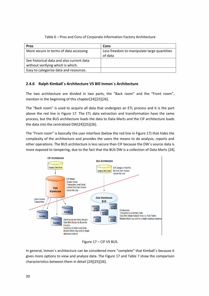
2.4.6 Ralph Kimball´s Architecture VS Bill Inmon´s Architecture
The two architecture are divided in two parts, the ”Back room” and the “Front room”,
mention in the beginning of this chapter[24][25][26].
The “Back room” is used to acquire all data that undergoes an ETL process and it is the part
above the red line in Figure 17. The ETL data extraction and transformation have the same
process, but the BUS architecture loads the data to Data Marts and the CIF architecture loads
the data into the centralized DW[24][25][26].
The “Front room” is basically the user interface (below the red line in Figure 17) that hides the
complexity of the architecture and provides the users the means to do analysis, reports and
other operations. The BUS architecture is less secure than CIF because the DW´s source data is
more exposed to tampering, due to the fact that the BUS DW is a collection of Data Marts [24].
Figure 17 – CIF VS BUS.
In general, Inmon´s architecture can be considered more “complete” that Kimball´s because it
gives more options to view and analyze data. The Figure 17 and Table 7 show the comparison
characteristics between them in detail [24][25][26].
21
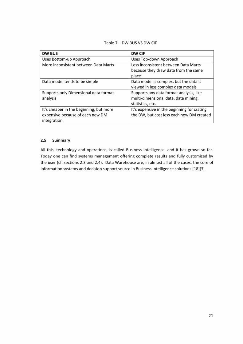
Table 7 – DW BUS VS DW CIF
DW BUS DW CIF
Uses Bottom-up Approach Uses Top-down Approach
More inconsistent between Data Marts Less inconsistent between Data Marts because they draw data from the same place
Data model tends to be simple Data model is complex, but the data is viewed in less complex data models
Supports only Dimensional data format analysis
Supports any data format analysis, like multi-dimensional data, data mining, statistics, etc.
It’s cheaper in the beginning, but more expensive because of each new DM integration
It’s expensive in the beginning for crating the DW, but cost less each new DM created
2.5 Summary
All this, technology and operations, is called Business Intelligence, and it has grown so far.
Today one can find systems management offering complete results and fully customized by
the user (cf. sections 2.3 and 2.4). Data Warehouse are, in almost all of the cases, the core of
information systems and decision support source in Business Intelligence solutions [18][3].

22
23
3 Linked Data
In this chapter, it is presented the possible formats that the result data produced by the semi-
automated process can have.
3.1 Linked Data Principles
The Internet is a global scale system that uses network devices to link other devices, by using
TCP/IP communication protocols. Also, the internet is a “vast” and “wild” reality, where
information can be stored and shared from those devices [34].
A human being is capable of perceive relationships between different sets of data, due to his
physical sensors and mental reasoning [35][36]. A machine doesn’t have that kind of
perception so it will need to have some “assistance” in to recognize those relations between
data. That is the main objective of Linked Data and Linked Open Data [5][6][7][8].
Tim Berners-Lee stated four design principles necessary to standardize the data structure that
is going to be used to publicize Linked Data repositories. They are [5][6][7][8]:
1. Using URIs to identify things because is a good way to identify and separate things.
For example, identify and separate two Life Expectancies studies (Study1 and Study2).
Study1 has the URI “Observations/obs1” and Study2 has the URI “Observations/obs2”;
2. Using HTTP URIs to be used as references for users and agents to access a thing
because most of them are in the web.
For example, references for the two Life Expectancies studies (Study1 and Study2):
Study1 – http://example.org/Observations#obs1;
Study2 – http://example.org/Observations#obs2;
3. The URI most have useful information in a format (RDF, OWL, SPARQL, SKOS, etc)
because it helps represent and publish the data.
24
4. Have URI Links to other related information because it helps represent and publish
the data. For example, to relate Study1(“http://example.org/Observations#obs1”)
with the 2004-2006 period (“http://example.org/Period#2004_2006“):
“http://example.org#hasTiePeriodID”
This principles, according to Tim Berners-Lee, can be transformed into 3 simple rules [6]:
1. All URI start with “http://” because LOD uses HTTP protocols;
2. All information must be published in a standard format (RDF and SPARQL for example);
3. All relations between thing must start with http://”, except literal values. For example,
Study1 life expectancy value (“http://example.org#lifeExpectancy”) is 76.
Any language or technology that uses Linked Data principles, like RDF and OWL can be
represented in a graph model, in which the data are nodes and the links are the unidirectional
edges that connect to other data nodes.
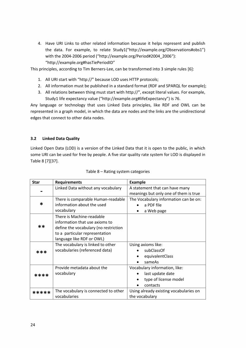
3.2 Linked Data Quality
Linked Open Data (LOD) is a version of the Linked Data that it is open to the public, in which
some URI can be used for free by people. A five star quality rate system for LOD is displayed in
Table 8 [7][37].
Table 8 – Rating system categories
Star Requirements Example
- Linked Data without any vocabulary A statement that can have many
meanings but only one of them is true
* There is comparable Human-readable information about the used vocabulary
The Vocabulary information can be on:
a PDF file
a Web page
**
There is Machine-readable information that use axioms to define the vocabulary (no restriction to a particular representation language like RDF or OWL)
***
The vocabulary is linked to other vocabularies (referenced data)
Using axioms like:
subClassOf
equivalentClass
sameAs
****
Provide metadata about the vocabulary
Vocabulary information, like:
last update date
type of license model
contacts
***** The vocabulary is connected to other vocabularies
Using already existing vocabularies on the vocabulary
25
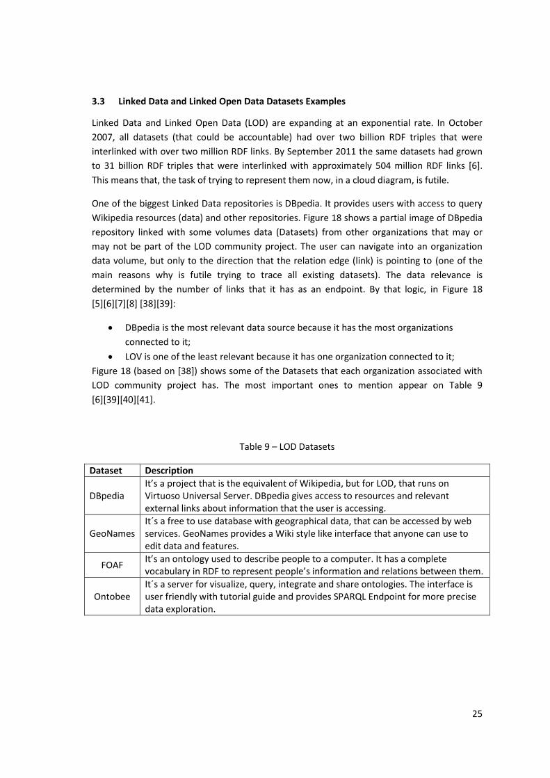
3.3 Linked Data and Linked Open Data Datasets Examples
Linked Data and Linked Open Data (LOD) are expanding at an exponential rate. In October
2007, all datasets (that could be accountable) had over two billion RDF triples that were
interlinked with over two million RDF links. By September 2011 the same datasets had grown
to 31 billion RDF triples that were interlinked with approximately 504 million RDF links [6].
This means that, the task of trying to represent them now, in a cloud diagram, is futile.
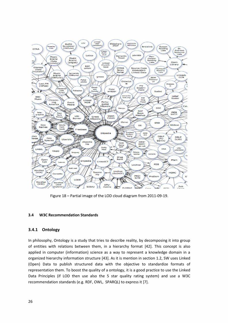
One of the biggest Linked Data repositories is DBpedia. It provides users with access to query
Wikipedia resources (data) and other repositories. Figure 18 shows a partial image of DBpedia
repository linked with some volumes data (Datasets) from other organizations that may or
may not be part of the LOD community project. The user can navigate into an organization
data volume, but only to the direction that the relation edge (link) is pointing to (one of the
main reasons why is futile trying to trace all existing datasets). The data relevance is
determined by the number of links that it has as an endpoint. By that logic, in Figure 18
[5][6][7][8] [38][39]:
DBpedia is the most relevant data source because it has the most organizations
connected to it;
LOV is one of the least relevant because it has one organization connected to it;
Figure 18 (based on [38]) shows some of the Datasets that each organization associated with
LOD community project has. The most important ones to mention appear on Table 9
[6][39][40][41].
Table 9 – LOD Datasets
Dataset Description
DBpedia It’s a project that is the equivalent of Wikipedia, but for LOD, that runs on Virtuoso Universal Server. DBpedia gives access to resources and relevant external links about information that the user is accessing.
GeoNames It´s a free to use database with geographical data, that can be accessed by web services. GeoNames provides a Wiki style like interface that anyone can use to edit data and features.
FOAF It’s an ontology used to describe people to a computer. It has a complete vocabulary in RDF to represent people’s information and relations between them.
Ontobee It´s a server for visualize, query, integrate and share ontologies. The interface is user friendly with tutorial guide and provides SPARQL Endpoint for more precise data exploration.
26
Figure 18 – Partial image of the LOD cloud diagram from 2011-09-19.
3.4 W3C Recommendation Standards
3.4.1 Ontology
In philosophy, Ontology is a study that tries to describe reality, by decomposing it into group
of entities with relations between them, in a hierarchy format [42]. This concept is also
applied in computer (information) science as a way to represent a knowledge domain in a
organized hierarchy information structure [43]. As it is mention in section 1.2, SW uses Linked
(Open) Data to publish structured data with the objective to standardize formats of
representation them. To boost the quality of a ontology, it is a good practice to use the Linked
Data Principles (if LOD then use also the 5 star quality rating system) and use a W3C
recommendation standards (e.g. RDF, OWL, SPARQL) to express it [7].
27
Independently of how ontologies are expressed, they share many identical structural features.
Their common components are [44]:
Classes – they represent concepts;
Individuals – they are instances (data) of the Classes in the ontology;
Attributes – they are the parameters that Classes and Individuals can have (e.g.
Properties);
Relations – they are way in which Classes and Individuals are linked;
Axioms – they are logical assertions that are used to describe the ontology domain
application;
Restrictions – they state how the data is used or represented in a ontology;
Function terms – they are complex structures implicated in certain relations that can
be used to replace an Individual term in a statement;
Rules – they are statements in a If-Then format that describes the logical inferences to
discover new data;
Events – are changing’s suffered by ontologies in a given time.
3.4.2 Resource Description Framework
Resource Description Framework (RDF) is an abstract and standard data model to describe
existing resources, it is a World Wide Web Consortium (W3C) recommendation to interchange
and represent data on the Web [4].
RDF Schema or RDFS is a structure of RDF resources (set of classes and properties) that do
basic description of ontologies by using RDF vocabularies. Some of the vocabularies
characteristics applied to an ontology are [45]:
Each existing resource (entity) is also a Uniform Resource Identifier (URI) because it
gives them a unique identification;
Each URI can be expressed and connected in groups of three URI (Triples);
Each Triple contains a subject, a predicate and a object (like a simple phrase);
A URI can be a Class that represents the concept of a resource;
A URI can be a Property that is used to define a Class or a instance of a Class;
A subject can be a Class or a instance of a Class;
A predicate can be a Property or a instance of a Property;
An object can be a class or an instance of a class or a Literal (Unicode string with no
URI).
The logical structure of RDF is a directed and labeled graph that can be expressed using
serializations like RDF/XML, N-Triples, Turtle, TriG, RDFa, Notation3 (N3), etc [4][46] [47].
28
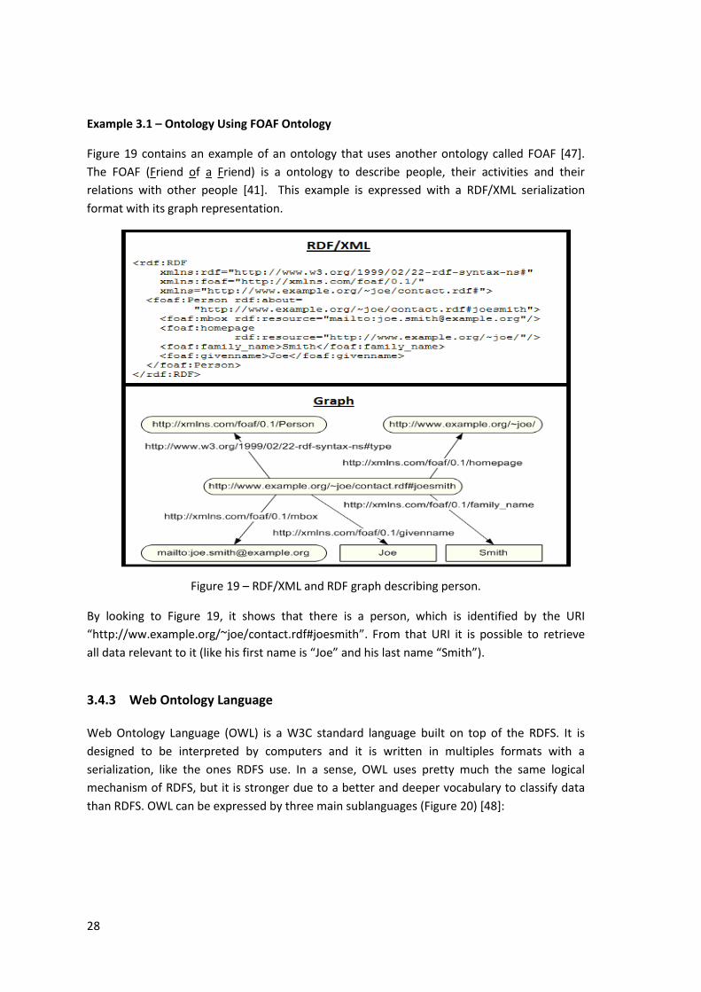
Example 3.1 – Ontology Using FOAF Ontology
Figure 19 contains an example of an ontology that uses another ontology called FOAF [47].
The FOAF (Friend of a Friend) is a ontology to describe people, their activities and their
relations with other people [41]. This example is expressed with a RDF/XML serialization
format with its graph representation.
Figure 19 – RDF/XML and RDF graph describing person.
By looking to Figure 19, it shows that there is a person, which is identified by the URI
“http://ww.example.org/~joe/contact.rdf#joesmith”. From that URI it is possible to retrieve
all data relevant to it (like his first name is “Joe” and his last name “Smith”).
3.4.3 Web Ontology Language
Web Ontology Language (OWL) is a W3C standard language built on top of the RDFS. It is
designed to be interpreted by computers and it is written in multiples formats with a
serialization, like the ones RDFS use. In a sense, OWL uses pretty much the same logical
mechanism of RDFS, but it is stronger due to a better and deeper vocabulary to classify data
than RDFS. OWL can be expressed by three main sublanguages (Figure 20) [48]:
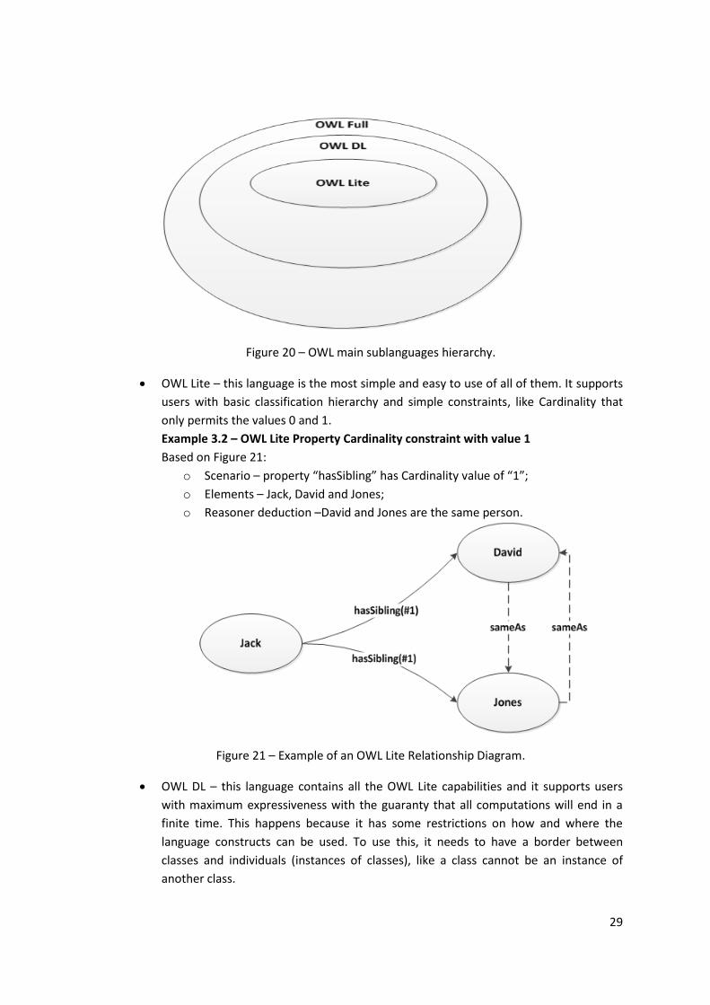
29
Figure 20 – OWL main sublanguages hierarchy.
OWL Lite – this language is the most simple and easy to use of all of them. It supports
users with basic classification hierarchy and simple constraints, like Cardinality that
only permits the values 0 and 1.
Example 3.2 – OWL Lite Property Cardinality constraint with value 1
Based on Figure 21:
o Scenario – property “hasSibling” has Cardinality value of “1”;
o Elements – Jack, David and Jones;
o Reasoner deduction –David and Jones are the same person.
Figure 21 – Example of an OWL Lite Relationship Diagram.
OWL DL – this language contains all the OWL Lite capabilities and it supports users
with maximum expressiveness with the guaranty that all computations will end in a
finite time. This happens because it has some restrictions on how and where the
language constructs can be used. To use this, it needs to have a border between
classes and individuals (instances of classes), like a class cannot be an instance of
another class.
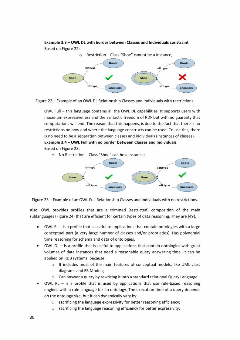
30
Example 3.3 – OWL DL with border between Classes and Individuals constraint
Based on Figure 22:
o Restriction – Class “Shoe” cannot be a Instance;
Figure 22 – Example of an OWL DL Relationship Classes and Individuals with restrictions.
OWL Full – this language contains all the OWL DL capabilities. It supports users with
maximum expressiveness and the syntactic freedom of RDF but with no guaranty that
computations will end. The reason that this happens, is due to the fact that there is no
restrictions on how and where the language constructs can be used. To use this, there
is no need to be a separation between classes and individuals (instances of classes).
Example 3.4 – OWL Full with no border between Classes and Individuals
Based on Figure 23:
o No Restriction – Class “Shoe” can be a Instance;
Figure 23 – Example of an OWL Full Relationship Classes and Individuals with no restrictions.
Also, OWL provides profiles that are a trimmed (restricted) composition of the main
sublanguages (Figure 24) that are efficient for certain types of data reasoning. They are [49]:
OWL EL – is a profile that is useful to applications that contain ontologies with a large
conceptual part (a very large number of classes and/or proprieties). Has polynomial
time reasoning for schema and data of ontologies.
OWL QL – is a profile that is useful to applications that contain ontologies with great
volumes of data instances that need a reasonable query answering time. It can be
applied on RDB systems, because:
o It includes most of the main features of conceptual models, like UML class
diagrams and ER Models;
o Can answer a query by rewriting it into a standard relational Query Language.
OWL RL – is a profile that is used by applications that use rule-based reasoning
engines with a rule language for an ontology. The execution time of a query depends
on the ontology size, but it can dynamically vary by:
o sacrificing the language expressivity for better reasoning efficiency;
o sacrificing the language reasoning efficiency for better expressivity;
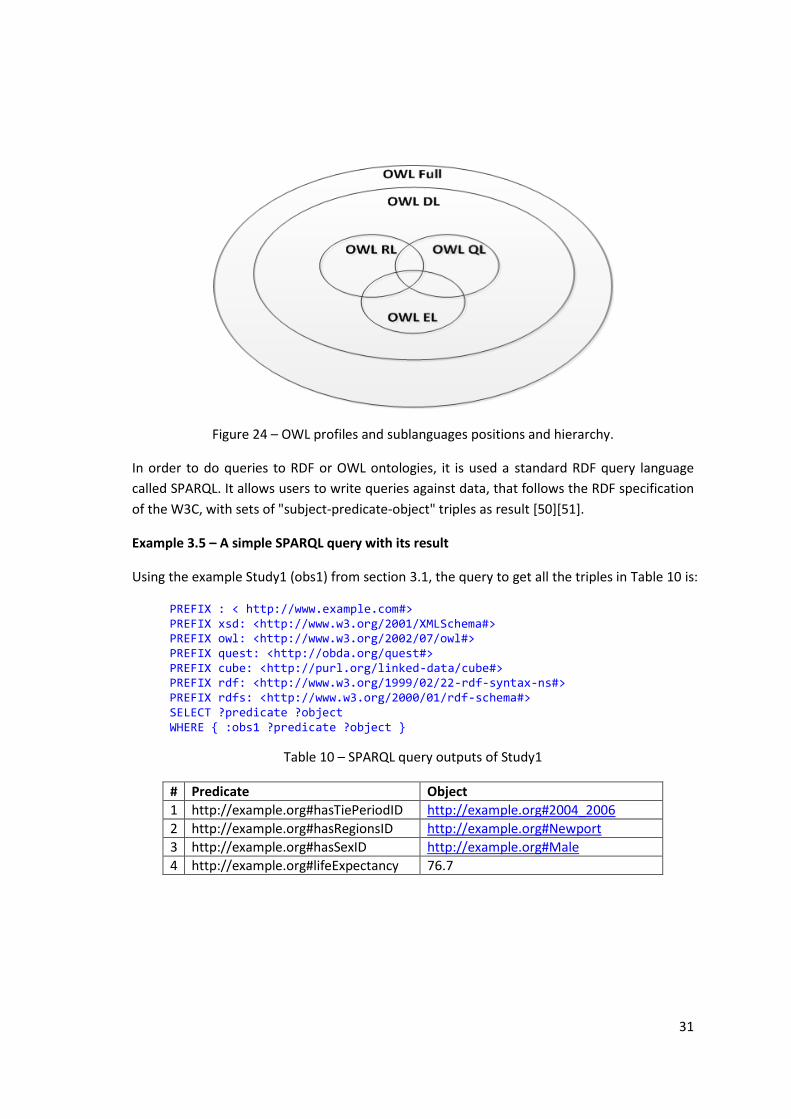
31
Figure 24 – OWL profiles and sublanguages positions and hierarchy.
In order to do queries to RDF or OWL ontologies, it is used a standard RDF query language
called SPARQL. It allows users to write queries against data, that follows the RDF specification
of the W3C, with sets of "subject-predicate-object" triples as result [50][51].
Example 3.5 – A simple SPARQL query with its result
Using the example Study1 (obs1) from section 3.1, the query to get all the triples in Table 10 is:
PREFIX : < http://www.example.com#> PREFIX xsd: <http://www.w3.org/2001/XMLSchema#> PREFIX owl: <http://www.w3.org/2002/07/owl#> PREFIX quest: <http://obda.org/quest#> PREFIX cube: <http://purl.org/linked-data/cube#> PREFIX rdf: <http://www.w3.org/1999/02/22-rdf-syntax-ns#> PREFIX rdfs: <http://www.w3.org/2000/01/rdf-schema#> SELECT ?predicate ?object WHERE { :obs1 ?predicate ?object }
Table 10 – SPARQL query outputs of Study1
# Predicate Object
1 http://example.org#hasTiePeriodID http://example.org#2004_2006
2 http://example.org#hasRegionsID http://example.org#Newport
3 http://example.org#hasSexID http://example.org#Male
4 http://example.org#lifeExpectancy 76.7
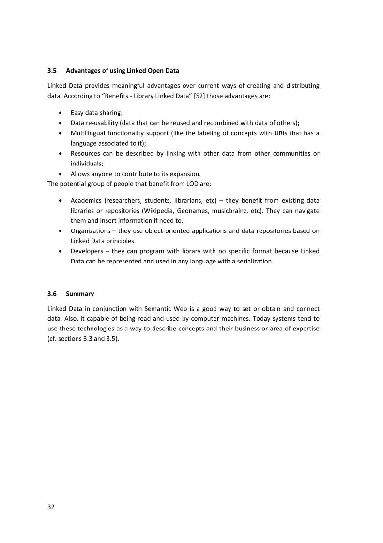
32
3.5 Advantages of using Linked Open Data
Linked Data provides meaningful advantages over current ways of creating and distributing
data. According to “Benefits - Library Linked Data” [52] those advantages are:
Easy data sharing;
Data re-usability (data that can be reused and recombined with data of others);
Multilingual functionality support (like the labeling of concepts with URIs that has a
language associated to it);
Resources can be described by linking with other data from other communities or
individuals;
Allows anyone to contribute to its expansion.
The potential group of people that benefit from LOD are:
Academics (researchers, students, librarians, etc) – they benefit from existing data
libraries or repositories (Wikipedia, Geonames, musicbrainz, etc). They can navigate
them and insert information if need to.
Organizations – they use object-oriented applications and data repositories based on
Linked Data principles.
Developers – they can program with library with no specific format because Linked
Data can be represented and used in any language with a serialization.
3.6 Summary
Linked Data in conjunction with Semantic Web is a good way to set or obtain and connect
data. Also, it capable of being read and used by computer machines. Today systems tend to
use these technologies as a way to describe concepts and their business or area of expertise
(cf. sections 3.3 and 3.5).
33
4 RDB to RDF Languages
In this chapter, it is presented the information needed for the semi-automated to convert the
data from the source DW to the result RDF Cube.
4.1 RDB to RDF mapping
The applications and technologies of SW are recent, which means that a lot of data on the
Internet doesn't benefit from their abilities, e.g. the data on Relational Databases. The types
of data that have the desired format are Linked Data. So a way to use Relational Database
(RDB) data is to map it into RDF or similar [48].
The general idea of mapping RDB into RDF is to transform the RDB records into a RDF
Graph[54]. Also this increases the interoperability between the two Data Models, making the
possibility of using RDB to extract or store the data of any SW technology or application
[55][53] .
Then there are different ways of accessing the new RDF data (Figure 25):
by using a query language like SPARQL;
by using a HTTP GET of a URI on the RDF graph;
by getting the data from a Triplestore (e.g. cf. RDF store in Figure 25)[56];
A representation of the idea, from RDB to RDF, can be seen in Figure 25 [54].
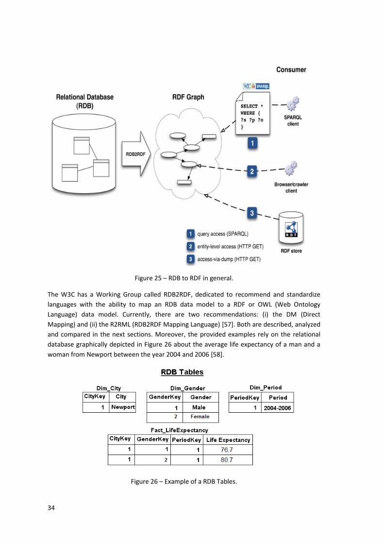
34
Figure 25 – RDB to RDF in general.
The W3C has a Working Group called RDB2RDF, dedicated to recommend and standardize
languages with the ability to map an RDB data model to a RDF or OWL (Web Ontology
Language) data model. Currently, there are two recommendations: (i) the DM (Direct
Mapping) and (ii) the R2RML (RDB2RDF Mapping Language) [57]. Both are described, analyzed
and compared in the next sections. Moreover, the provided examples rely on the relational
database graphically depicted in Figure 26 about the average life expectancy of a man and a
woman from Newport between the year 2004 and 2006 [58].
Figure 26 – Example of a RDB Tables.
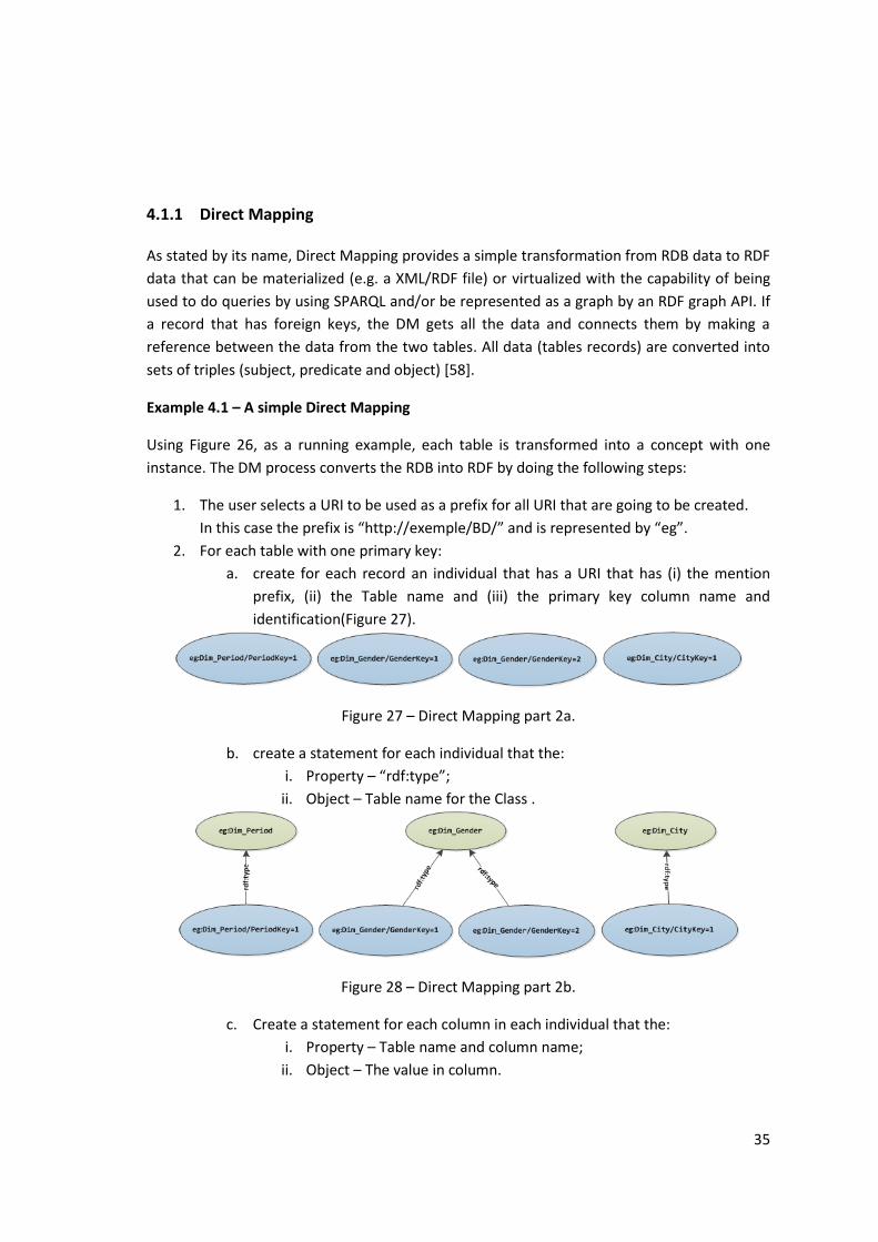
35
4.1.1 Direct Mapping
As stated by its name, Direct Mapping provides a simple transformation from RDB data to RDF
data that can be materialized (e.g. a XML/RDF file) or virtualized with the capability of being
used to do queries by using SPARQL and/or be represented as a graph by an RDF graph API. If
a record that has foreign keys, the DM gets all the data and connects them by making a
reference between the data from the two tables. All data (tables records) are converted into
sets of triples (subject, predicate and object) [58].
Example 4.1 – A simple Direct Mapping
Using Figure 26, as a running example, each table is transformed into a concept with one
instance. The DM process converts the RDB into RDF by doing the following steps:
1. The user selects a URI to be used as a prefix for all URI that are going to be created.
In this case the prefix is “http://exemple/BD/” and is represented by “eg”.
2. For each table with one primary key:
a. create for each record an individual that has a URI that has (i) the mention
prefix, (ii) the Table name and (iii) the primary key column name and
identification(Figure 27).
Figure 27 – Direct Mapping part 2a.
b. create a statement for each individual that the:
i. Property – “rdf:type”;
ii. Object – Table name for the Class .
Figure 28 – Direct Mapping part 2b.
c. Create a statement for each column in each individual that the:
i. Property – Table name and column name;
ii. Object – The value in column.
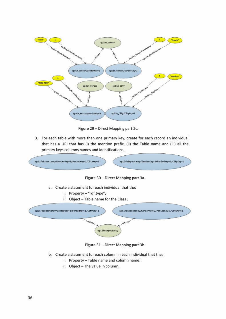
36
Figure 29 – Direct Mapping part 2c.
3. For each table with more than one primary key, create for each record an individual
that has a URI that has (i) the mention prefix, (ii) the Table name and (iii) all the
primary keys columns names and identifications.
Figure 30 – Direct Mapping part 3a.
a. Create a statement for each individual that the:
i. Property – “rdf:type”;
ii. Object – Table name for the Class .
Figure 31 – Direct Mapping part 3b.
b. Create a statement for each column in each individual that the:
i. Property – Table name and column name;
ii. Object – The value in column.
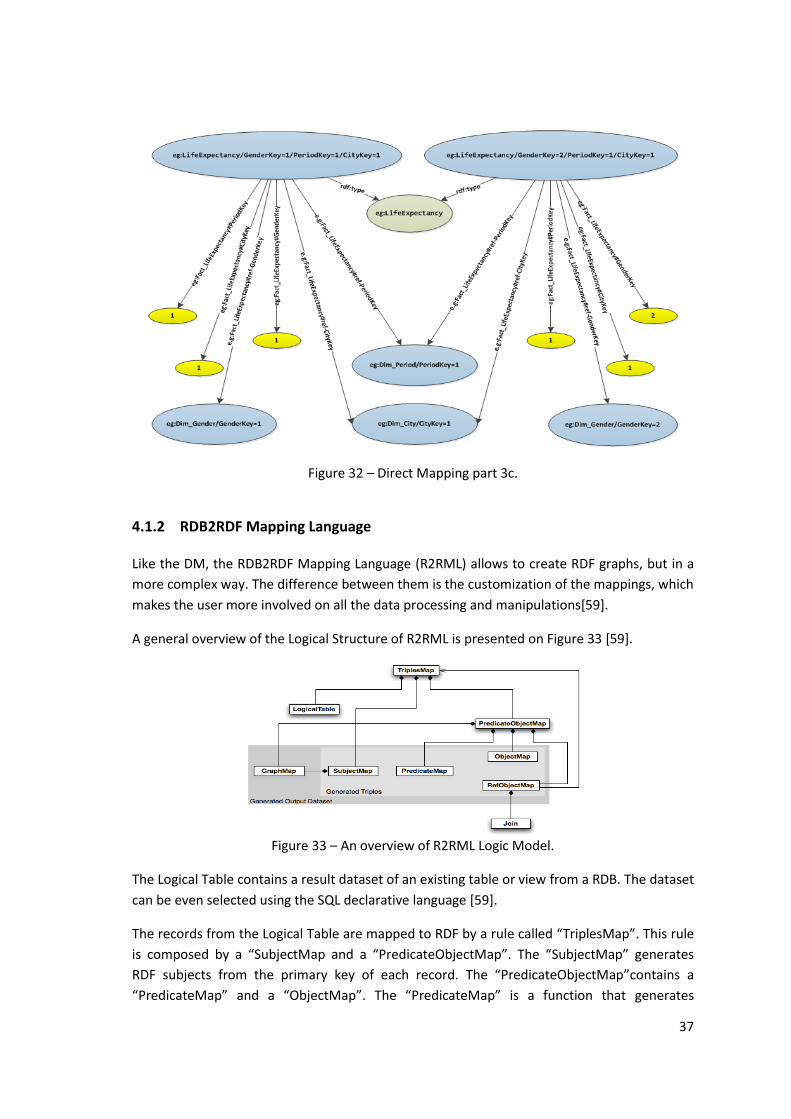
37
Figure 32 – Direct Mapping part 3c.
4.1.2 RDB2RDF Mapping Language
Like the DM, the RDB2RDF Mapping Language (R2RML) allows to create RDF graphs, but in a
more complex way. The difference between them is the customization of the mappings, which
makes the user more involved on all the data processing and manipulations[59].
A general overview of the Logical Structure of R2RML is presented on Figure 33 [59].
Figure 33 – An overview of R2RML Logic Model.
The Logical Table contains a result dataset of an existing table or view from a RDB. The dataset
can be even selected using the SQL declarative language [59].
The records from the Logical Table are mapped to RDF by a rule called “TriplesMap”. This rule
is composed by a “SubjectMap and a “PredicateObjectMap”. The “SubjectMap” generates
RDF subjects from the primary key of each record. The “PredicateObjectMap”contains a
“PredicateMap” and a “ObjectMap”. The “PredicateMap” is a function that generates
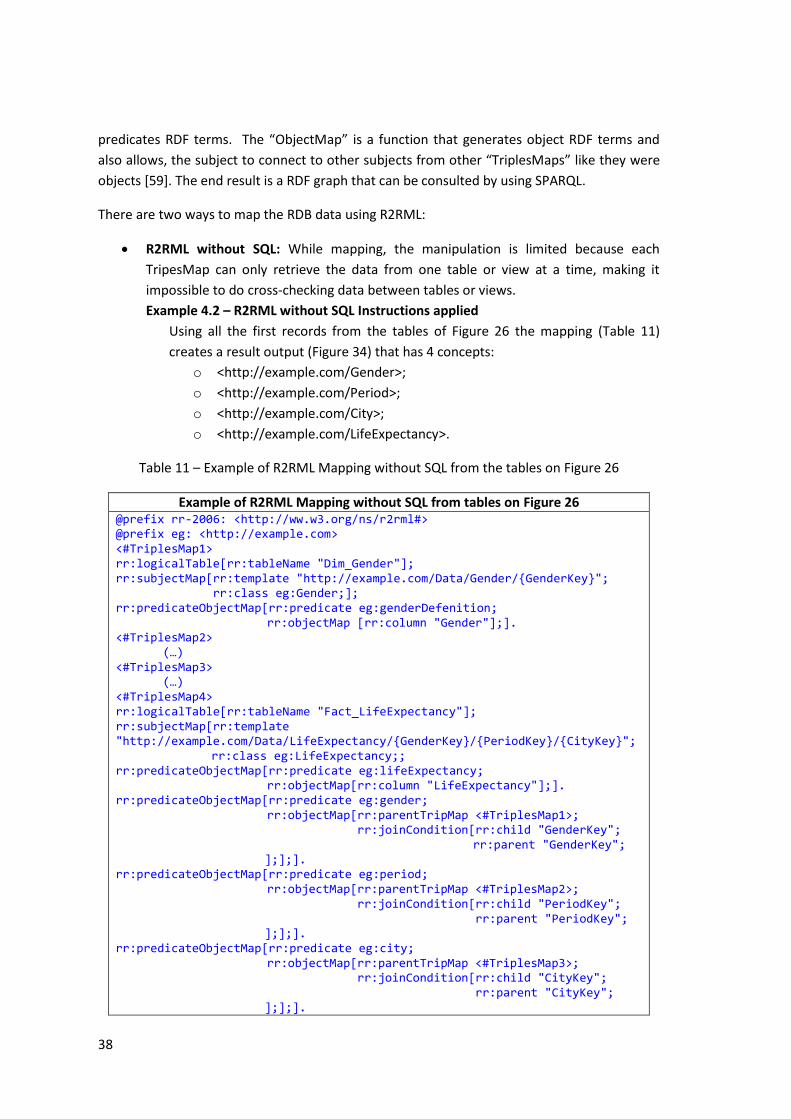
38
predicates RDF terms. The “ObjectMap” is a function that generates object RDF terms and
also allows, the subject to connect to other subjects from other “TriplesMaps” like they were
objects [59]. The end result is a RDF graph that can be consulted by using SPARQL.
There are two ways to map the RDB data using R2RML:
R2RML without SQL: While mapping, the manipulation is limited because each
TripesMap can only retrieve the data from one table or view at a time, making it
impossible to do cross-checking data between tables or views.
Example 4.2 – R2RML without SQL Instructions applied
Using all the first records from the tables of Figure 26 the mapping (Table 11)
creates a result output (Figure 34) that has 4 concepts:
o <http://example.com/Gender>;
o <http://example.com/Period>;
o <http://example.com/City>;
o <http://example.com/LifeExpectancy>.
Table 11 – Example of R2RML Mapping without SQL from the tables on Figure 26
Example of R2RML Mapping without SQL from tables on Figure 26 @prefix rr-2006: <http://ww.w3.org/ns/r2rml#> @prefix eg: <http://example.com> <#TriplesMap1> rr:logicalTable[rr:tableName "Dim_Gender"]; rr:subjectMap[rr:template "http://example.com/Data/Gender/{GenderKey}"; rr:class eg:Gender;]; rr:predicateObjectMap[rr:predicate eg:genderDefenition;
rr:objectMap [rr:column "Gender"];]. <#TriplesMap2> (…) <#TriplesMap3>
(…) <#TriplesMap4> rr:logicalTable[rr:tableName "Fact_LifeExpectancy"]; rr:subjectMap[rr:template "http://example.com/Data/LifeExpectancy/{GenderKey}/{PeriodKey}/{CityKey}";
rr:class eg:LifeExpectancy;; rr:predicateObjectMap[rr:predicate eg:lifeExpectancy;
rr:objectMap[rr:column "LifeExpectancy"];]. rr:predicateObjectMap[rr:predicate eg:gender;
rr:objectMap[rr:parentTripMap <#TriplesMap1>; rr:joinCondition[rr:child "GenderKey"; rr:parent "GenderKey"; ];];].
rr:predicateObjectMap[rr:predicate eg:period; rr:objectMap[rr:parentTripMap <#TriplesMap2>; rr:joinCondition[rr:child "PeriodKey"; rr:parent "PeriodKey"; ];];].
rr:predicateObjectMap[rr:predicate eg:city; rr:objectMap[rr:parentTripMap <#TriplesMap3>; rr:joinCondition[rr:child "CityKey"; rr:parent "CityKey"; ];];].
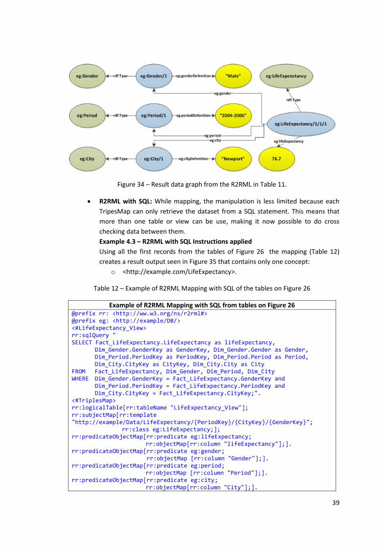
39
Figure 34 – Result data graph from the R2RML in Table 11.
R2RML with SQL: While mapping, the manipulation is less limited because each
TripesMap can only retrieve the dataset from a SQL statement. This means that
more than one table or view can be use, making it now possible to do cross
checking data between them.
Example 4.3 – R2RML with SQL Instructions applied
Using all the first records from the tables of Figure 26 the mapping (Table 12)
creates a result output seen in Figure 35 that contains only one concept:
o <http://example.com/LifeExpectancy>.
Table 12 – Example of R2RML Mapping with SQL of the tables on Figure 26
Example of R2RML Mapping with SQL from tables on Figure 26 @prefix rr: <http://ww.w3.org/ns/r2rml#> @prefix eg: <http://example/DB/> <#LifeExpectancy_View> rr:sqlQuery " SELECT Fact_LifeExpectancy.LifeExpectancy as lifeExpectancy,
Dim_Gender.GenderKey as GenderKey, Dim_Gender.Gender as Gender, Dim_Period.PeriodKey as PeriodKey, Dim_Period.Period as Period, Dim_City.CityKey as CityKey, Dim_City.City as City
FROM Fact_LifeExpectancy, Dim_Gender, Dim_Period, Dim_City WHERE Dim_Gender.GenderKey = Fact_LifeExpectancy.GenderKey and
Dim_Period.PeriodKey = Fact_LifeExpectancy.PeriodKey and Dim_City.CityKey = Fact_LifeExpectancy.CityKey;".
<#TriplesMap> rr:logicalTable[rr:tableName "LifeExpectancy_View"]; rr:subjectMap[rr:template "http://example/Data/LifeExpectancy/{PeriodKey}/{CityKey}/{GenderKey}";
rr:class eg:LifeExpectancy;]; rr:predicateObjectMap[rr:predicate eg:lifeExpectancy;
rr:objectMap[rr:column "lifeExpectancy"];]. rr:predicateObjectMap[rr:predicate eg:gender; rr:objectMap [rr:column "Gender"];]. rr:predicateObjectMap[rr:predicate eg:period;
rr:objectMap [rr:column "Period"];]. rr:predicateObjectMap[rr:predicate eg:city;
rr:objectMap[rr:column "City"];].
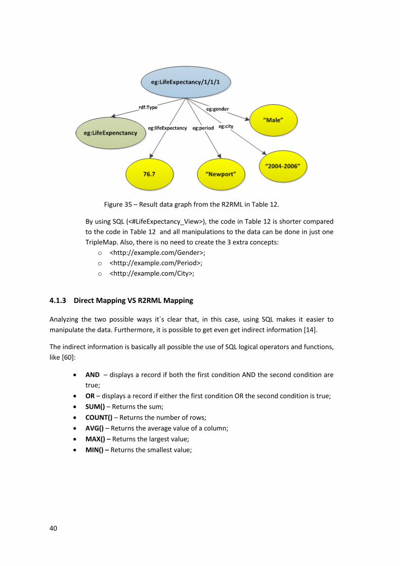
40
Figure 35 – Result data graph from the R2RML in Table 12.
By using SQL (<#LifeExpectancy_View>), the code in Table 12 is shorter compared
to the code in Table 12 and all manipulations to the data can be done in just one
TripleMap. Also, there is no need to create the 3 extra concepts:
o <http://example.com/Gender>;
o <http://example.com/Period>;
o <http://example.com/City>;
4.1.3 Direct Mapping VS R2RML Mapping
Analyzing the two possible ways it´s clear that, in this case, using SQL makes it easier to
manipulate the data. Furthermore, it is possible to get even get indirect information [14].
The indirect information is basically all possible the use of SQL logical operators and functions,
like [60]:
AND – displays a record if both the first condition AND the second condition are
true;
OR – displays a record if either the first condition OR the second condition is true;
SUM() – Returns the sum;
COUNT() – Returns the number of rows;
AVG() – Returns the average value of a column;
MAX() – Returns the largest value;
MIN() – Returns the smallest value;
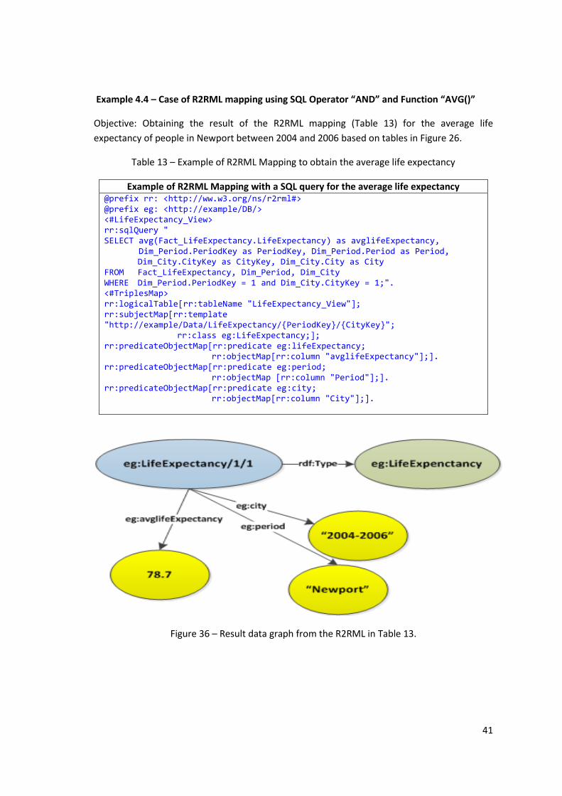
41
Example 4.4 – Case of R2RML mapping using SQL Operator “AND” and Function “AVG()”
Objective: Obtaining the result of the R2RML mapping (Table 13) for the average life
expectancy of people in Newport between 2004 and 2006 based on tables in Figure 26.
Table 13 – Example of R2RML Mapping to obtain the average life expectancy
Example of R2RML Mapping with a SQL query for the average life expectancy @prefix rr: <http://ww.w3.org/ns/r2rml#> @prefix eg: <http://example/DB/> <#LifeExpectancy_View> rr:sqlQuery " SELECT avg(Fact_LifeExpectancy.LifeExpectancy) as avglifeExpectancy, Dim_Period.PeriodKey as PeriodKey, Dim_Period.Period as Period, Dim_City.CityKey as CityKey, Dim_City.City as City FROM Fact_LifeExpectancy, Dim_Period, Dim_City WHERE Dim_Period.PeriodKey = 1 and Dim_City.CityKey = 1;". <#TriplesMap> rr:logicalTable[rr:tableName "LifeExpectancy_View"]; rr:subjectMap[rr:template "http://example/Data/LifeExpectancy/{PeriodKey}/{CityKey}";
rr:class eg:LifeExpectancy;]; rr:predicateObjectMap[rr:predicate eg:lifeExpectancy;
rr:objectMap[rr:column "avglifeExpectancy"];]. rr:predicateObjectMap[rr:predicate eg:period;
rr:objectMap [rr:column "Period"];]. rr:predicateObjectMap[rr:predicate eg:city; rr:objectMap[rr:column "City"];].
Figure 36 – Result data graph from the R2RML in Table 13.
42
4.2 Other RDB to RDF mapping Languages
The W3C standard languages are the DM and R2RML, but there are other languages and
technologies that allow RDB to RDF mappings. Some of them are [61][62]:
The eD2R [63] – It is an extension of D2R MAP ( a declarative, XML-based RDB to RDF
mapping language) that has the objective of mapping databases with simple
structures;
R2O [64] – It is an extensible and full declarative language that uses XML-based syntax
for mapping complex RDB into RDF or OWL;
Relacional.OWL [65] – “is a technique to automatically extract the semantics” of
relational databases and turn the result information into RDF/OWL;
Virtuoso [66] – It is "a middleware and database engine hybrid that combines the
functionality of traditional RDBMS, ORDBMS, virtual database, RDF, XML, free-text,
web application server and file server" in a universal server. It maps SQL data to
Linked Data Views and the result data is access by SPARQL ;
D2RQ [67] – It is a platform and declarative mapping language that can access the
resulting RDF/OWL data by SPARQL;
Triplify [68] – It is a plug-in for web applications that creates semantic structures from
RDB and gives the result in RDF, JSON and Linked Data;
R3M [69] – It is bidirectional RDB to RDF mapping language of OntoAccess mediation
platform, with update-awareness capability;
Ultrawrap [10][70][71] – It is a optimized system that can match relational databases
scalability because it can execute SPARQ statements as fast as SQL statements. Also,
it implements all the W3C RDB2RDF Standards, Direct Mapping and R2RML, for the
“RDF graph representation of the relational data”.
ontop [72] – “is a platform to query databases as Virtual RDF Graphs using SPARQL.
It's extremely fast and is packed with features”. Has its own language structure and
can read and write in R2RML language. Also it is free to use.
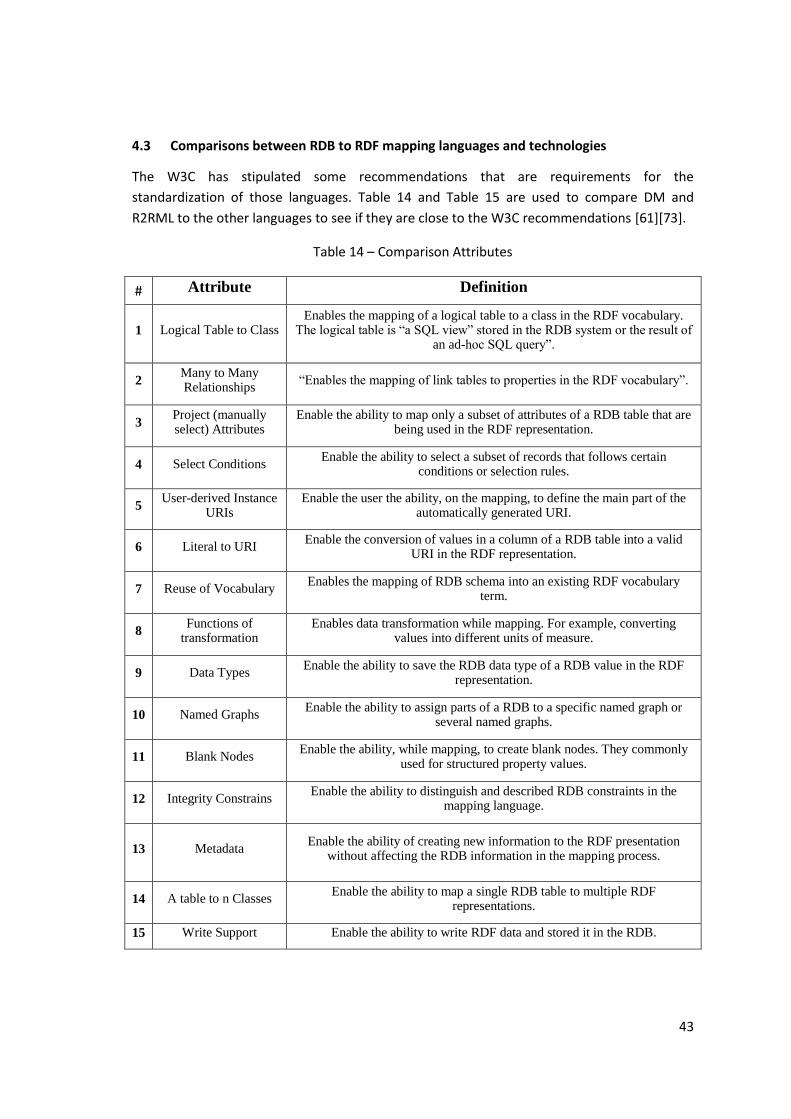
43
4.3 Comparisons between RDB to RDF mapping languages and technologies
The W3C has stipulated some recommendations that are requirements for the
standardization of those languages. Table 14 and Table 15 are used to compare DM and
R2RML to the other languages to see if they are close to the W3C recommendations [61][73].
Table 14 – Comparison Attributes
# Attribute Definition
1 Logical Table to Class Enables the mapping of a logical table to a class in the RDF vocabulary.
The logical table is “a SQL view” stored in the RDB system or the result of an ad-hoc SQL query”.
2 Many to Many Relationships
“Enables the mapping of link tables to properties in the RDF vocabulary”.
3 Project (manually select) Attributes
Enable the ability to map only a subset of attributes of a RDB table that are being used in the RDF representation.
4 Select Conditions Enable the ability to select a subset of records that follows certain
conditions or selection rules.
5 User-derived Instance
URIs Enable the user the ability, on the mapping, to define the main part of the
automatically generated URI.
6 Literal to URI Enable the conversion of values in a column of a RDB table into a valid
URI in the RDF representation.
7 Reuse of Vocabulary Enables the mapping of RDB schema into an existing RDF vocabulary
term.
8 Functions of
transformation Enables data transformation while mapping. For example, converting
values into different units of measure.
9 Data Types Enable the ability to save the RDB data type of a RDB value in the RDF
representation.
10 Named Graphs Enable the ability to assign parts of a RDB to a specific named graph or
several named graphs.
11 Blank Nodes Enable the ability, while mapping, to create blank nodes. They commonly
used for structured property values.
12 Integrity Constrains Enable the ability to distinguish and described RDB constraints in the
mapping language.
13 Metadata Enable the ability of creating new information to the RDF presentation
without affecting the RDB information in the mapping process.
14 A table to n Classes Enable the ability to map a single RDB table to multiple RDF
representations.
15 Write Support Enable the ability to write RDF data and stored it in the RDB.
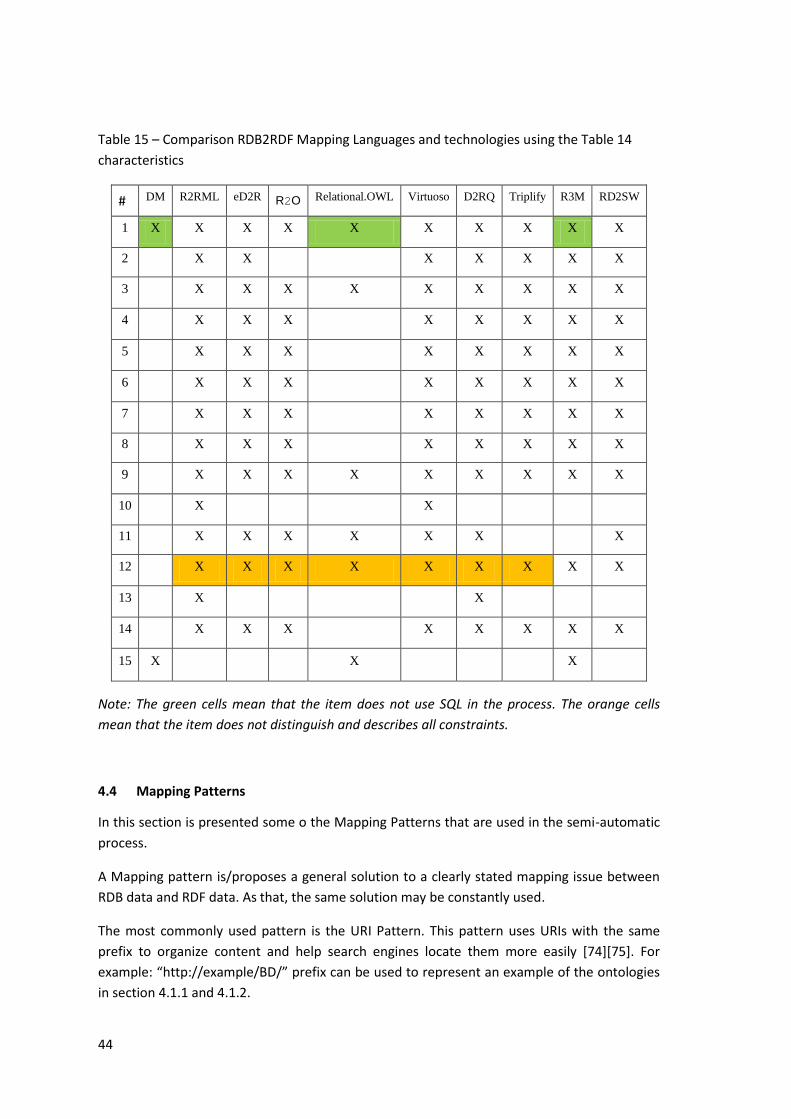
44
Table 15 – Comparison RDB2RDF Mapping Languages and technologies using the Table 14
characteristics
# DM R2RML eD2R R2O Relational.OWL Virtuoso D2RQ Triplify R3M RD2SW
1 X X X X X X X X X X
2 X X X X X X X
3 X X X X X X X X X
4 X X X X X X X X
5 X X X X X X X X
6 X X X X X X X X
7 X X X X X X X X
8 X X X X X X X X
9 X X X X X X X X X
10 X X
11 X X X X X X X
12 X X X X X X X X X
13 X X
14 X X X X X X X X
15 X X X
Note: The green cells mean that the item does not use SQL in the process. The orange cells
mean that the item does not distinguish and describes all constraints.
4.4 Mapping Patterns
In this section is presented some o the Mapping Patterns that are used in the semi-automatic
process.
A Mapping pattern is/proposes a general solution to a clearly stated mapping issue between
RDB data and RDF data. As that, the same solution may be constantly used.
The most commonly used pattern is the URI Pattern. This pattern uses URIs with the same
prefix to organize content and help search engines locate them more easily [74][75]. For
example: “http://example/BD/” prefix can be used to represent an example of the ontologies
in section 4.1.1 and 4.1.2.
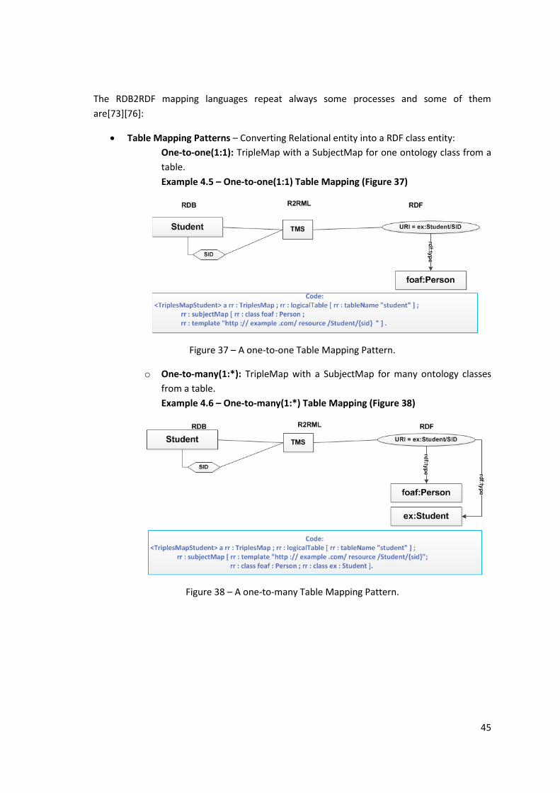
45
The RDB2RDF mapping languages repeat always some processes and some of them
are[73][76]:
Table Mapping Patterns – Converting Relational entity into a RDF class entity:
One-to-one(1:1): TripleMap with a SubjectMap for one ontology class from a
table.
Example 4.5 – One-to-one(1:1) Table Mapping (Figure 37)
Figure 37 – A one-to-one Table Mapping Pattern.
o One-to-many(1:*): TripleMap with a SubjectMap for many ontology classes
from a table.
Example 4.6 – One-to-many(1:*) Table Mapping (Figure 38)
Figure 38 – A one-to-many Table Mapping Pattern.
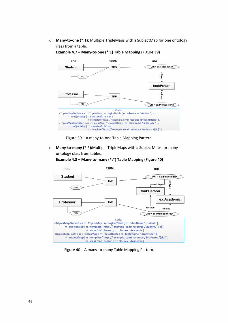
46
o Many-to-one (*:1): Multiple TripleMaps with a SubjectMap for one ontology
class from a table.
Example 4.7 – Many-to-one (*:1) Table Mapping (Figure 39)
Figure 39 – A many-to-one Table Mapping Pattern.
o Many-to-many (*:*):Multiple TripleMaps with a SubjectMaps for many
ontology class from tables.
Example 4.8 – Many-to-many (*:*) Table Mapping (Figure 40)
Figure 40 – A many-to-many Table Mapping Pattern.
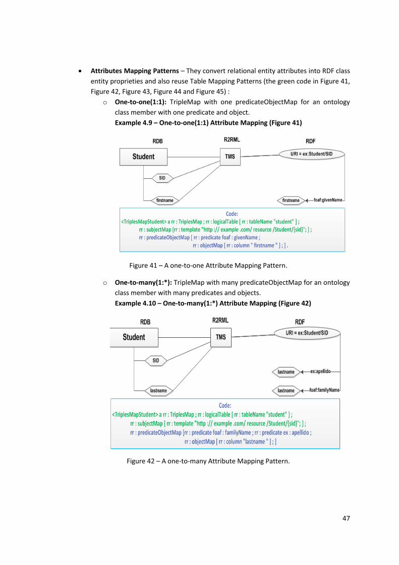
47
Attributes Mapping Patterns – They convert relational entity attributes into RDF class
entity proprieties and also reuse Table Mapping Patterns (the green code in Figure 41,
Figure 42, Figure 43, Figure 44 and Figure 45) :
o One-to-one(1:1): TripleMap with one predicateObjectMap for an ontology
class member with one predicate and object.
Example 4.9 – One-to-one(1:1) Attribute Mapping (Figure 41)
Figure 41 – A one-to-one Attribute Mapping Pattern.
o One-to-many(1:*): TripleMap with many predicateObjectMap for an ontology
class member with many predicates and objects.
Example 4.10 – One-to-many(1:*) Attribute Mapping (Figure 42)
Figure 42 – A one-to-many Attribute Mapping Pattern.
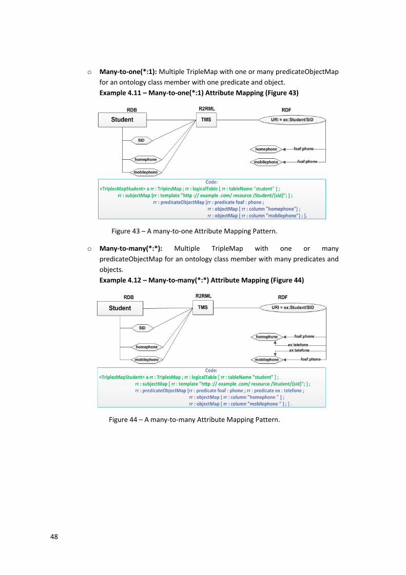
48
o Many-to-one(*:1): Multiple TripleMap with one or many predicateObjectMap
for an ontology class member with one predicate and object.
Example 4.11 – Many-to-one(*:1) Attribute Mapping (Figure 43)
Figure 43 – A many-to-one Attribute Mapping Pattern.
o Many-to-many(*:*): Multiple TripleMap with one or many
predicateObjectMap for an ontology class member with many predicates and
objects.
Example 4.12 – Many-to-many(*:*) Attribute Mapping (Figure 44)
Figure 44 – A many-to-many Attribute Mapping Pattern.
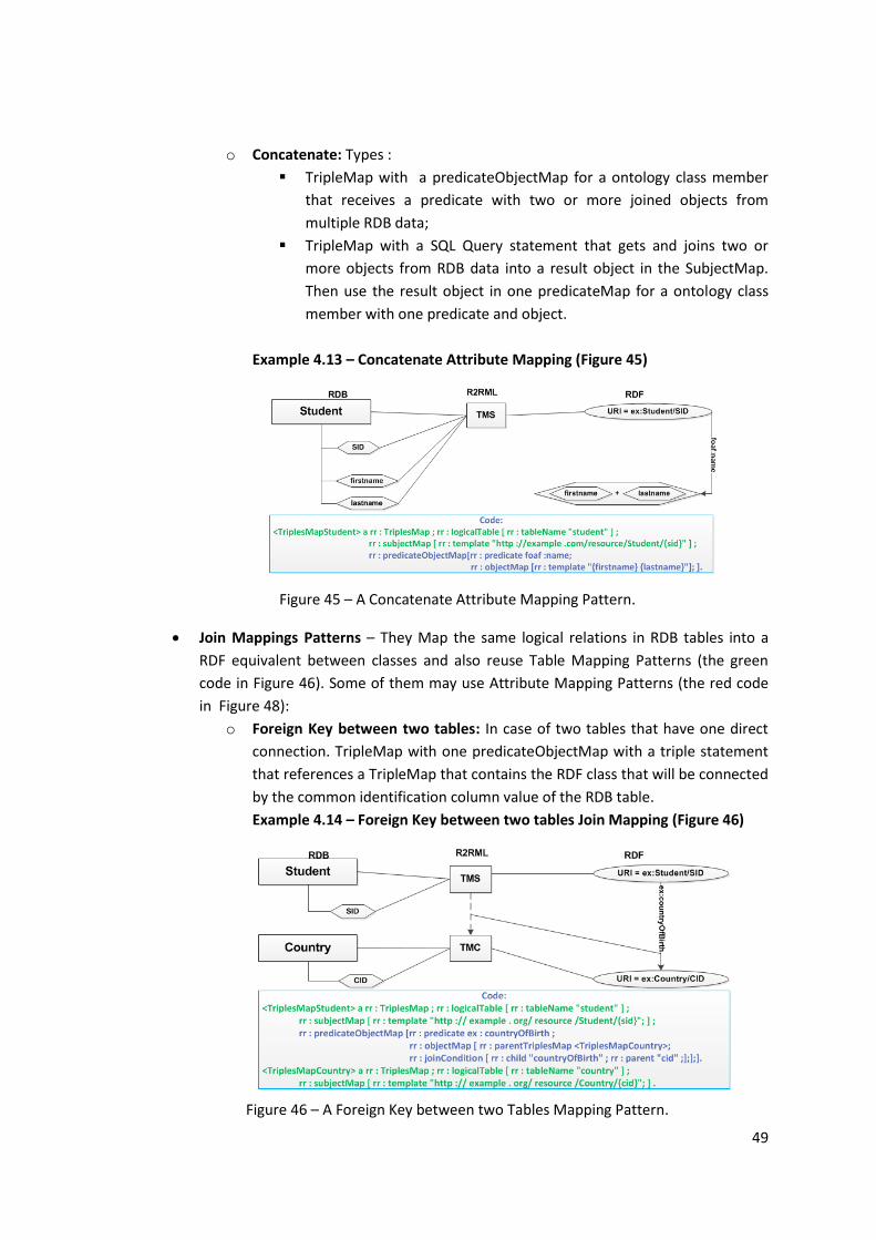
49
o Concatenate: Types :
TripleMap with a predicateObjectMap for a ontology class member
that receives a predicate with two or more joined objects from
multiple RDB data;
TripleMap with a SQL Query statement that gets and joins two or
more objects from RDB data into a result object in the SubjectMap.
Then use the result object in one predicateMap for a ontology class
member with one predicate and object.
Example 4.13 – Concatenate Attribute Mapping (Figure 45)
Figure 45 – A Concatenate Attribute Mapping Pattern.
Join Mappings Patterns – They Map the same logical relations in RDB tables into a
RDF equivalent between classes and also reuse Table Mapping Patterns (the green
code in Figure 46). Some of them may use Attribute Mapping Patterns (the red code
in Figure 48):
o Foreign Key between two tables: In case of two tables that have one direct
connection. TripleMap with one predicateObjectMap with a triple statement
that references a TripleMap that contains the RDF class that will be connected
by the common identification column value of the RDB table.
Example 4.14 – Foreign Key between two tables Join Mapping (Figure 46)
Figure 46 – A Foreign Key between two Tables Mapping Pattern.
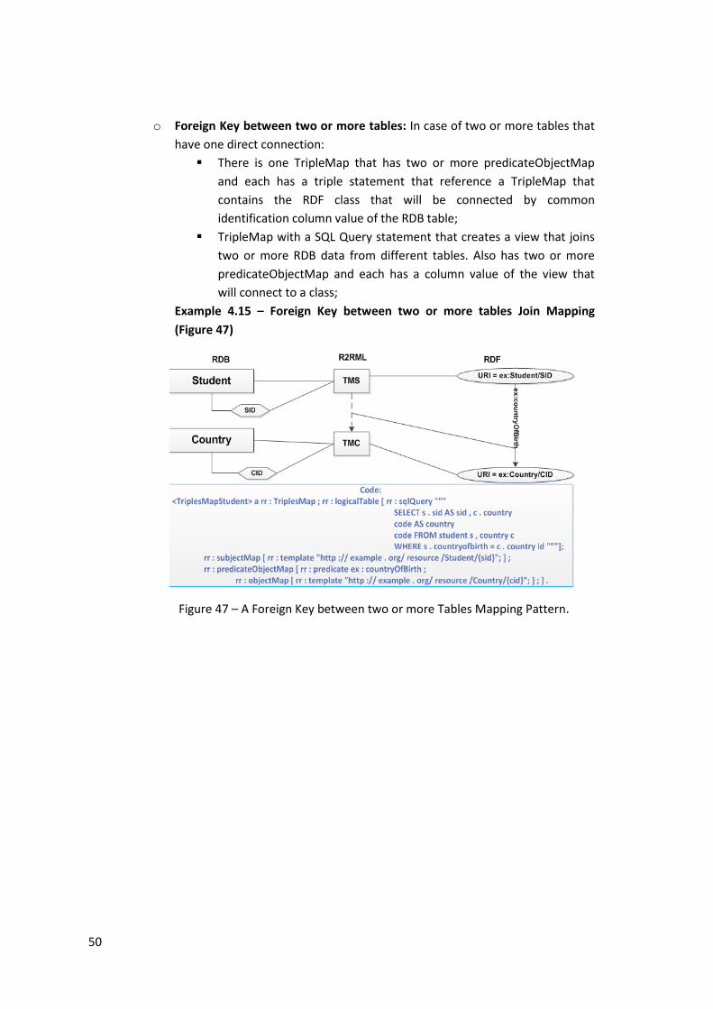
50
o Foreign Key between two or more tables: In case of two or more tables that
have one direct connection:
There is one TripleMap that has two or more predicateObjectMap
and each has a triple statement that reference a TripleMap that
contains the RDF class that will be connected by common
identification column value of the RDB table;
TripleMap with a SQL Query statement that creates a view that joins
two or more RDB data from different tables. Also has two or more
predicateObjectMap and each has a column value of the view that
will connect to a class;
Example 4.15 – Foreign Key between two or more tables Join Mapping
(Figure 47)
Figure 47 – A Foreign Key between two or more Tables Mapping Pattern.
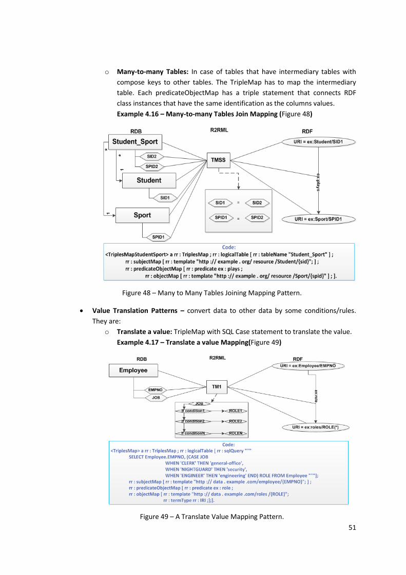
51
o Many-to-many Tables: In case of tables that have intermediary tables with
compose keys to other tables. The TripleMap has to map the intermediary
table. Each predicateObjectMap has a triple statement that connects RDF
class instances that have the same identification as the columns values.
Example 4.16 – Many-to-many Tables Join Mapping (Figure 48)
Figure 48 – Many to Many Tables Joining Mapping Pattern.
Value Translation Patterns – convert data to other data by some conditions/rules.
They are:
o Translate a value: TripleMap with SQL Case statement to translate the value.
Example 4.17 – Translate a value Mapping(Figure 49)
Figure 49 – A Translate Value Mapping Pattern.
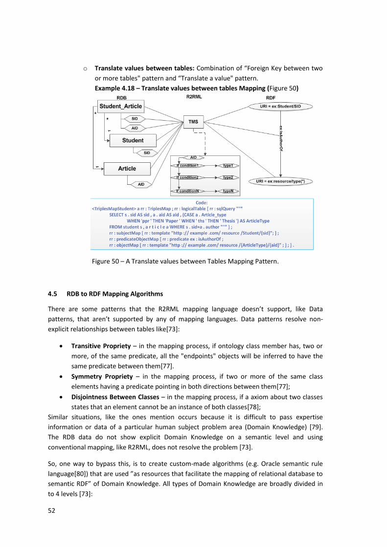
52
o Translate values between tables: Combination of “Foreign Key between two
or more tables" pattern and “Translate a value" pattern.
Example 4.18 – Translate values between tables Mapping (Figure 50)
Figure 50 – A Translate values between Tables Mapping Pattern.
4.5 RDB to RDF Mapping Algorithms
There are some patterns that the R2RML mapping language doesn’t support, like Data
patterns, that aren’t supported by any of mapping languages. Data patterns resolve non-
explicit relationships between tables like[73]:
Transitive Propriety – in the mapping process, if ontology class member has, two or
more, of the same predicate, all the "endpoints" objects will be inferred to have the
same predicate between them[77].
Symmetry Propriety – in the mapping process, if two or more of the same class
elements having a predicate pointing in both directions between them[77];
Disjointness Between Classes – in the mapping process, if a axiom about two classes
states that an element cannot be an instance of both classes[78];
Similar situations, like the ones mention occurs because it is difficult to pass expertise
information or data of a particular human subject problem area (Domain Knowledge) [79].
The RDB data do not show explicit Domain Knowledge on a semantic level and using
conventional mapping, like R2RML, does not resolve the problem [73].
So, one way to bypass this, is to create custom-made algorithms (e.g. Oracle semantic rule
language[80]) that are used ”as resources that facilitate the mapping of relational database to
semantic RDF” of Domain Knowledge. All types of Domain Knowledge are broadly divided in
to 4 levels [73]:
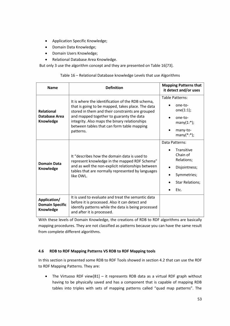
53
Application Specific Knowledge;
Domain Data Knowledge;
Domain Users Knowledge;
Relational Database Area Knowledge.
But only 3 use the algorithm concept and they are presented on Table 16[73].
Table 16 – Relational Database knowledge Levels that use Algorithms
Name Definition Mapping Patterns that it detect and/or uses
Relational Database Area Knowledge
It is where the identification of the RDB schema, that is going to be mapped, takes place. The data stored in them and their constraints are grouped and mapped together to guaranty the data integrity. Also maps the binary relationships between tables that can form table mapping patterns.
Table Patterns:
one-to-one(1:1);
one-to-many(1:*);
many-to-many(*:*);
Domain Data Knowledge
It “describes how the domain data is used to represent knowledge in the mapped RDF Schema” and as well the non-explicit relationships between tables that are normally represented by languages like OWL.
Data Patterns:
Transitive Chain of Relations;
Disjointness;
Symmetries;
Star Relations;
Etc.
Application/ Domain Specific Knowledge
It is used to evaluate and treat the semantic data before it is processed. Also it can detect and identify patterns while the data is being processed and after it is processed.
With these levels of Domain Knowledge, the creations of RDB to RDF algorithms are basically
mapping procedures. They are not classified as patterns because you can have the same result
from complete different algorithms.
4.6 RDB to RDF Mapping Patterns VS RDB to RDF Mapping tools
In this section is presented some RDB to RDF Tools showed in section 4.2 that can use the RDF
to RDF Mapping Patterns. They are:
The Virtuoso RDF view[81] – it represents RDB data as a virtual RDF graph without
having to be physically saved and has a component that is capable of mapping RDB
tables into triples with sets of mapping patterns called “quad map patterns”. The
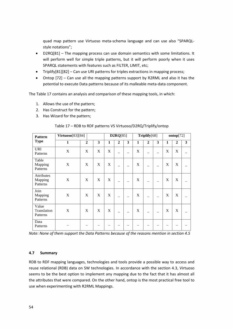
54
quad map pattern use Virtuoso meta-schema language and can use also “SPARQL-
style notations”;
D2RQ[81] – The mapping process can use domain semantics with some limitations. It
will perform well for simple triple patterns, but it will perform poorly when it uses
SPARQL statements with features such as FILTER, LIMIT, etc;
Triplify[81][82] – Can use URI patterns for triples extractions in mapping process;
Ontop [72] – Can use all the mapping patterns support by R2RML and also it has the
potential to execute Data patterns because of its malleable meta-data component.
The Table 17 contains an analysis and comparison of these mapping tools, in which:
1. Allows the use of the pattern;
2. Has Construct for the pattern;
3. Has Wizard for the pattern;
Table 17 – RDB to RDF patterns VS Virtuoso/D2RQ/Triplify/ontop
Pattern Type
Virtuoso[83][84] D2RQ[85] Triplify[68] ontop[72]
1 2 3 1 2 3 1 2 3 1 2 3
URI Patterns
X X X X _ _ X _ _ X X _
Table Mapping Patterns
X X X X _ _ X _ _ X X _
Attributes Mapping Patterns
X X X X _ _ X _ _ X X _
Join Mapping Patterns
X X X X _ _ X _ _ X X _
Value Translation Patterns
X X X X _ _ X _ _ X X _
Data Patterns
_ _ _ _ _ _ _ _ _ _ _ _
Note: None of them support the Data Patterns because of the reasons mention in section 4.5
4.7 Summary
RDB to RDF mapping languages, technologies and tools provide a possible way to access and
reuse relational (RDB) data on SW technologies. In accordance with the section 4.3, Virtuoso
seems to be the best option to implement any mapping due to the fact that it has almost all
the attributes that were compared. On the other hand, ontop is the most practical free tool to
use when experimenting with R2RML Mappings.
55
5 RDF Data Cube Vocabulary
In this chapter, it is presented the Vocabulary for the RDF Data Cube that the semi-automatic
process exploits.
The objective of RDF Data Cube vocabulary is to give the current existing RDF or OWL data a
multi-dimensional perspective, like statistical data. This chapter shows that using the RDF
Data Cube Vocabulary will enable the semi-automated process to output the resulting data in
a Dimensional Cube format. The vocabulary is a W3C recommendation [12], even though it
was develop and expanded by the Government Linked Data (GLD) Working Group.
5.1 Vocabulary Diagram and Elements
The RDF Data Cube Vocabulary is an ontology use to describe the concept of a Dimensional
Cube (cf. section 2.3) in a RDF format. The main purpose of this vocabulary is to allow that
data represented according to a given ontology can be interpreted as a Dimensional Cube too.
An ontology that uses instantiations of this vocabulary on already existing data, will gain the
RDF Data Cube capabilities and perspective. This means that all RDF Data Cubes that use this
iterations will also gain a standard usability functionality, independently of the business or
theme it is trying to express [12].
Figure 51 (from [12]) shows a diagram of the RDF Data Cube Vocabulary with the relations
between the Classes and the Properties where:
“qb” is the vocabulary URI prefix (“http://purl.org/linked-data/cube#”);
“skos” is the URI prefix for “a common data model for sharing and linking knowledge
organization systems” on the web [86], recommended by W3C, and it is use to define
a Class as a concept;
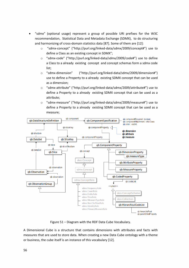
56
“sdmx” (optional usage) represent a group of possible URI prefixes for the W3C
recommendation, Statistical Data and Metadata Exchange (SDMX), to do structuring
and harmonizing of cross-domain statistics data [87]. Some of them are [12]:
o “sdmx-concept” (“http://purl.org/linked-data/sdmx/2009/concept#”) use to
define a Class as an existing concept in SDMX”;
o “sdmx-code” (“http://purl.org/linked-data/sdmx/2009/code#”) use to define
a Class to a already existing concept and concept schemas form a sdmx code
list;
o “sdmx-dimension” (“http://purl.org/linked-data/sdmx/2009/dimension#”)
use to define a Property to a already existing SDMX concept that can be used
as a dimension;
o “sdmx-attribute” (“http://purl.org/linked-data/sdmx/2009/attribute#”) use to
define a Property to a already existing SDMX concept that can be used as a
attribute;
o “sdmx-measure” (“http://purl.org/linked-data/sdmx/2009/measure#”) use to
define a Property to a already existing SDMX concept that can be used as a
measure;
Figure 51 – Diagram with the RDF Data Cube Vocabulary.
A Dimensional Cube is a structure that contains dimensions with attributes and facts with
measures that are used to store data. When creating a new Data Cube ontology with a theme
or business, the cube itself is an instance of this vocabulary [12].
57
A qb:DataSet individual (cf. Example 5.2) is a collection of statistical data of one type of fact
with measures that has a defined dimensional structure (qb:DataStructureDefinition
individual linked by the property qb:structure) dictating how the data is represented or
organized [12].
A qb:DataStructureDefinition individual (cf. Example 5.3) defines how qb:DataSet individual
and qb:Slice individual (via qb:SliceKey individuals) are structured and organized. To better
organized dimensions and measures, of the facts, it can be use qb:ComponentSpecification
individuals (linked by the property qb:component) to do a more detail organization structure
[12].
The qb:ComponentSpecification individuals (cf. Example 5.4 and Example 5.5) give a more
deep detail of how the dimensions and/or measures behave. Those details can be expressed
by using the property [12]:
qb:order – it is used to give the priority order in which the data is presented.
For example: if dimensions: city is 1, period is 2 and gender is 3. The presentation
order would be by city, then by period, then by gender;
qb:componentRequired – it is used to verify if a component (dimension or measure)
is required in the Data Structure Definition. If true, then it has to be used and if false
then it is considered as optional in a qb:DataStructureDefinition individual;
qb: componentAttachement – it is used to specify if a qb:ComponentProperty
individual is linked to another individual from a classes, like qb:DataSet, qb:Slice,
qb:Observation and MeasureProperty;
qb:dimension – is a property in which the endpoints are considered dimensions;
qb:attribute – is a property in which the endpoints are considered attributes;
qb:measure – is a property in which the endpoints are considered measures.
The qb:ComponentProperty is an abstract property class. A qb:ComponentSpecification
individual can be linked to qb:ComponentProperty individuals by the property
qb:componentProperty. If qb:ComponentProperty individuals have the need to be more
specific, they can use [12]:
qb:DimensionProperty to declare that it is a dimension property (cf. Example 5.6);
qb:AttributeProperty to declare that it is also a attribute property (cf. Example 5.8);
qb:MeasureProperty to declare that it is also a measure property (cf. Example 5.7);
qb:CodeProperty to declare that it is also a coded property. SKOS and SDMX code lists
can be applied here (cf. Example 5.9).
An Observation (qb:Observation individual) is a fact element data and also a small piece of a
Dataset (linked by the qb:dataset property). Has a group of dimensions and a group of
measures associated with it. The dimensions help to identify or find a Observation (fact), in
order to easily access its measures (cf. Example 5.10) [12].
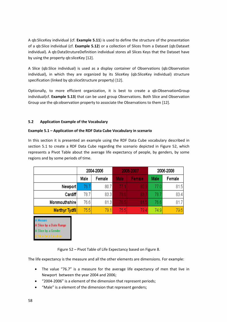
58
A qb:SliceKey individual (cf. Example 5.11) is used to define the structure of the presentation
of a qb:Slice individual (cf. Example 5.12) or a collection of Slices from a Dataset (qb:Dataset
individual). A qb:DataStrutureDefinition individual stores all Slices Keys that the Dataset have
by using the property qb:sliceKey [12].
A Slice (qb:Slice individual) is used as a display container of Observations (qb:Observation
individual), in which they are organized by its SliceKey (qb:SliceKey individual) structure
specification (linked by qb:sliceStructure property) [12].
Optionally, to more efficient organization, it is best to create a qb:ObservationGroup
individual(cf. Example 5.13) that can be used group Observations. Both Slice and Observation
Group use the qb:observation property to associate the Observations to them [12].
5.2 Application Example of the Vocabulary
Example 5.1 – Application of the RDF Data Cube Vocabulary in scenario
In this section it is presented an example using the RDF Data Cube vocabulary described in
section 5.1 to create a RDF Data Cube regarding the scenario depicted in Figure 52, which
represents a Pivot Table about the average life expectancy of people, by genders, by some
regions and by some periods of time.
Figure 52 – Pivot Table of Life Expectancy based on Figure 8.
The life expectancy is the measure and all the other elements are dimensions. For example:
The value “76.7” is a measure for the average life expectancy of men that live in
Newport between the year 2004 and 2006;
“2004-2006” is a element of the dimension that represent periods;
“Male” is a element of the dimension that represent genders;
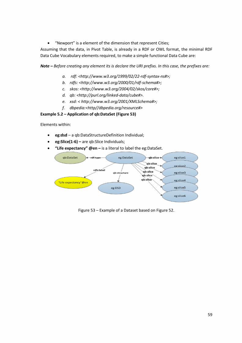
59
“Newport” is a element of the dimension that represent Cities;
Assuming that the data, in Pivot Table, is already in a RDF or OWL format, the minimal RDF
Data Cube Vocabulary elements required, to make a simple functional Data Cube are:
Note – Before creating any element its is declare the URI prefixs. In this case, the prefixes are:
a. rdf: <http://www.w3.org/1999/02/22-rdf-syntax-ns#>;
b. rdfs: <http://www.w3.org/2000/01/rdf-schema#>;
c. skos: <http://www.w3.org/2004/02/skos/core#>;
d. qb: <http://purl.org/linked-data/cube#>.
e. xsd: < http://www.w3.org/2001/XMLSchema#>;
f. dbpedia:<http//dbpedia.org/resource#>
Example 5.2 – Application of qb:DataSet (Figure 53)
Elements within:
eg:dsd – a qb:DataStructureDefinition Individual;
eg:Slice(1-6) – are qb:Slice Individuals;
“Life expectancy” @en – is a literal to label the eg:DataSet.
Figure 53 – Example of a Dataset based on Figure 52.
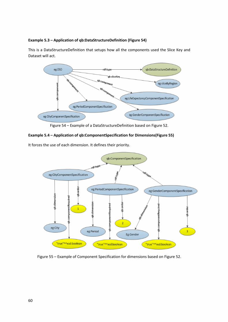
60
Example 5.3 – Application of qb:DataStructureDefinition (Figure 54)
This is a DataStructureDefinition that setups how all the components used the Slice Key and
Dataset will act.
Figure 54 – Example of a DataStructureDefinition based on Figure 52.
Example 5.4 – Application of qb:ComponentSpecification for Dimensions(Figure 55)
It forces the use of each dimension. It defines their priority.
Figure 55 – Example of Component Specification for dimensions based on Figure 52.
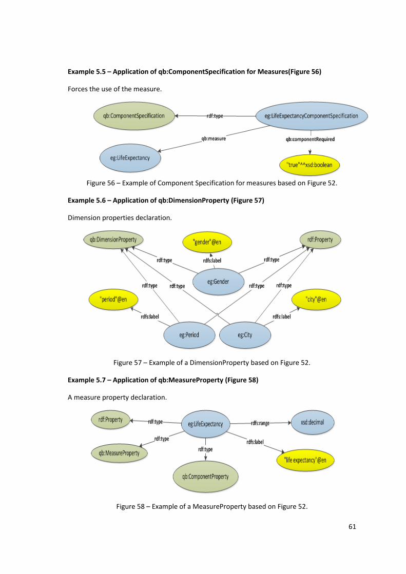
61
Example 5.5 – Application of qb:ComponentSpecification for Measures(Figure 56)
Forces the use of the measure.
Figure 56 – Example of Component Specification for measures based on Figure 52.
Example 5.6 – Application of qb:DimensionProperty (Figure 57)
Dimension properties declaration.
Figure 57 – Example of a DimensionProperty based on Figure 52.
Example 5.7 – Application of qb:MeasureProperty (Figure 58)
A measure property declaration.
Figure 58 – Example of a MeasureProperty based on Figure 52.
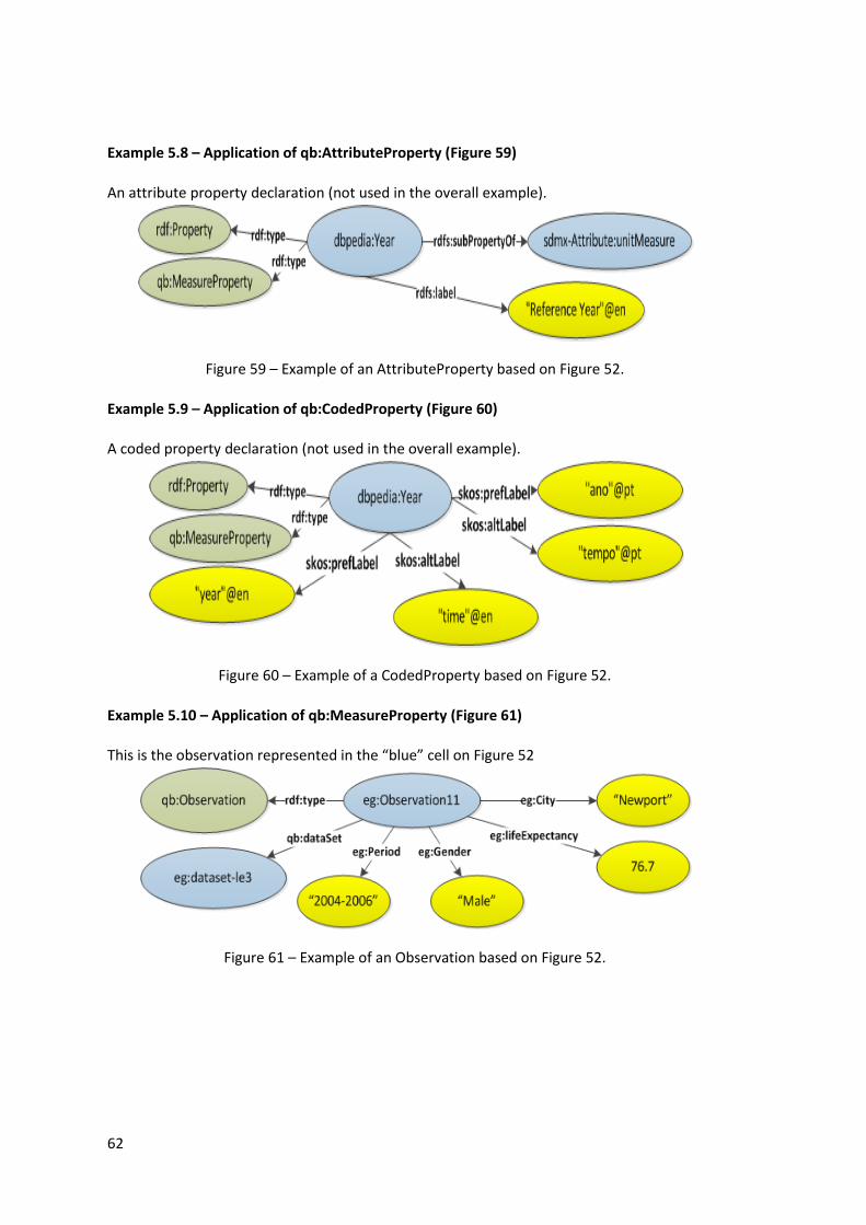
62
Example 5.8 – Application of qb:AttributeProperty (Figure 59)
An attribute property declaration (not used in the overall example).
Figure 59 – Example of an AttributeProperty based on Figure 52.
Example 5.9 – Application of qb:CodedProperty (Figure 60)
A coded property declaration (not used in the overall example).
Figure 60 – Example of a CodedProperty based on Figure 52.
Example 5.10 – Application of qb:MeasureProperty (Figure 61)
This is the observation represented in the “blue” cell on Figure 52
Figure 61 – Example of an Observation based on Figure 52.
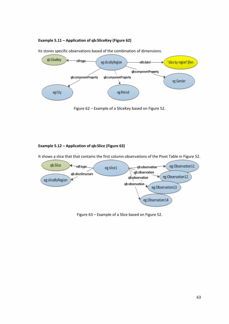
63
Example 5.11 – Application of qb:SliceKey (Figure 62)
Its stores specific observations based of the combination of dimensions.
Figure 62 – Example of a SliceKey based on Figure 52.
Example 5.12 – Application of qb:Slice (Figure 63)
It shows a slice that that contains the first column observations of the Pivot Table in Figure 52.
Figure 63 – Example of a Slice based on Figure 52.
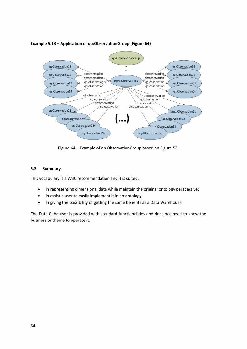
64
Example 5.13 – Application of qb:ObservationGroup (Figure 64)
Figure 64 – Example of an ObservationGroup based on Figure 52.
5.3 Summary
This vocabulary is a W3C recommendation and it is suited:
In representing dimensional data while maintain the original ontology perspective;
In assist a user to easily implement it in an ontology;
In giving the possibility of getting the same benefits as a Data Warehouse.
The Data Cube user is provided with standard functionalities and does not need to know the
business or theme to operate it.
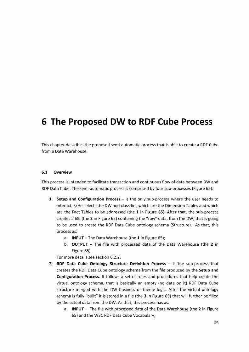
65
6 The Proposed DW to RDF Cube Process
This chapter describes the proposed semi-automatic process that is able to create a RDF Cube
from a Data Warehouse.
6.1 Overview
This process is intended to facilitate transaction and continuous flow of data between DW and
RDF Data Cube. The semi-automatic process is comprised by four sub-processes (Figure 65):
1. Setup and Configuration Process – is the only sub-process where the user needs to
interact. S/He selects the DW and classifies which are the Dimension Tables and which
are the Fact Tables to be addressed (the 1 in Figure 65). After that, the sub-process
creates a file (the 2 in Figure 65) containing the “raw” data, from the DW, that is going
to be used to create the RDF Data Cube ontology schema (Structure). As that, this
process as:
a. INPUT – The Data Warehouse (the 1 in Figure 65);
b. OUTPUT – The file with processed data of the Data Warehouse (the 2 in
Figure 65).
For more details see section 6.2.2.
2. RDF Data Cube Ontology Structure Definition Process – is the sub-process that
creates the RDF Data Cube ontology schema from the file produced by the Setup and
Configuration Process. It follows a set of rules and procedures that help create the
virtual ontology schema, that is basically an empty (no data on it) RDF Data Cube
structure merged with the DW business or theme logic. After the virtual ontology
schema is fully “built” it is stored in a file (the 3 in Figure 65) that will further be filled
by the actual data from the DW. As that, this process has as:
a. INPUT – The file with processed data of the Data Warehouse (the 2 in Figure
65) and the W3C RDF Data Cube Vocabulary;
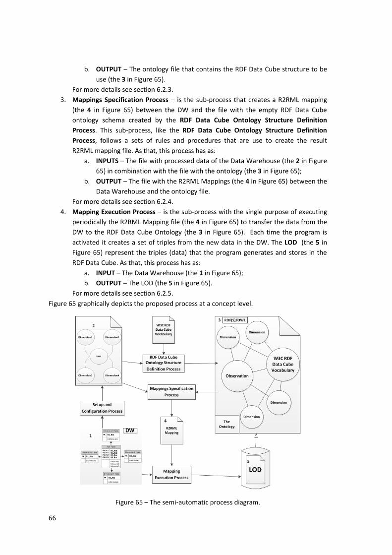
66
b. OUTPUT – The ontology file that contains the RDF Data Cube structure to be
use (the 3 in Figure 65).
For more details see section 6.2.3.
3. Mappings Specification Process – is the sub-process that creates a R2RML mapping
(the 4 in Figure 65) between the DW and the file with the empty RDF Data Cube
ontology schema created by the RDF Data Cube Ontology Structure Definition
Process. This sub-process, like the RDF Data Cube Ontology Structure Definition
Process, follows a sets of rules and procedures that are use to create the result
R2RML mapping file. As that, this process has as:
a. INPUTS – The file with processed data of the Data Warehouse (the 2 in Figure
65) in combination with the file with the ontology (the 3 in Figure 65);
b. OUTPUT – The file with the R2RML Mappings (the 4 in Figure 65) between the
Data Warehouse and the ontology file.
For more details see section 6.2.4.
4. Mapping Execution Process – is the sub-process with the single purpose of executing
periodically the R2RML Mapping file (the 4 in Figure 65) to transfer the data from the
DW to the RDF Data Cube Ontology (the 3 in Figure 65). Each time the program is
activated it creates a set of triples from the new data in the DW. The LOD (the 5 in
Figure 65) represent the triples (data) that the program generates and stores in the
RDF Data Cube. As that, this process has as:
a. INPUT – The Data Warehouse (the 1 in Figure 65);
b. OUTPUT – The LOD (the 5 in Figure 65).
For more details see section 6.2.5.
Figure 65 graphically depicts the proposed process at a concept level.
Figure 65 – The semi-automatic process diagram.
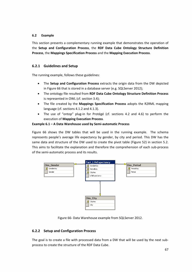
67
6.2 Example
This section presents a complementary running example that demonstrates the operation of
the Setup and Configuration Process, the RDF Data Cube Ontology Structure Definition
Process, the Mappings Specification Process and the Mapping Execution Process.
6.2.1 Guidelines and Setup
The running example, follows these guidelines:
The Setup and Configuration Process extracts the origin data from the DW depicted
in Figure 66 that is stored in a database server (e.g. SQLServer 2012);
The ontology file resulted from RDF Data Cube Ontology Structure Definition Process
is represented in OWL (cf. section 3.4);
The file created by the Mappings Specification Process adopts the R2RML mapping
language (cf. sections 4.1.2 and 4.1.3).
The use of “ontop” plug-in for Protégé (cf. sections 4.2 and 4.6) to perform the
execution of Mapping Execution Process.
Example 6.1 – A Data Warehouse used by Semi-automatic Process
Figure 66 shows the DW tables that will be used in the running example. The schema
represents people’s average life expectancy by gender, by city and period. This DW has the
same data and structure of the DW used to create the pivot table (Figure 52) in section 5.2.
This aims to facilitate the explanation and therefore the comprehension of each sub-process
of the semi-automatic process and its results.
Figure 66- Data Warehouse example from SQLServer 2012.
6.2.2 Setup and Configuration Process
The goal is to create a file with processed data from a DW that will be used by the next sub-
process to create the structure of the RDF Data Cube.
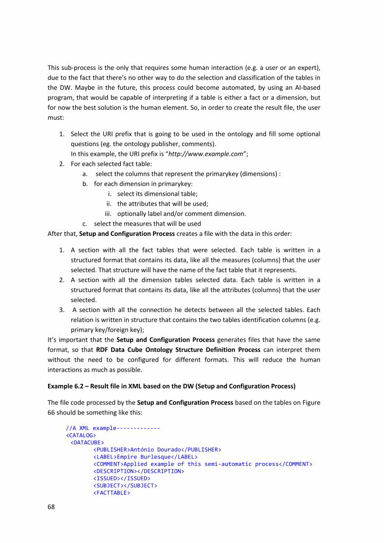
68
This sub-process is the only that requires some human interaction (e.g. a user or an expert),
due to the fact that there’s no other way to do the selection and classification of the tables in
the DW. Maybe in the future, this process could become automated, by using an AI-based
program, that would be capable of interpreting if a table is either a fact or a dimension, but
for now the best solution is the human element. So, in order to create the result file, the user
must:
1. Select the URI prefix that is going to be used in the ontology and fill some optional
questions (eg. the ontology publisher, comments).
In this example, the URI prefix is “http://www.example.com”;
2. For each selected fact table:
a. select the columns that represent the primarykey (dimensions) :
b. for each dimension in primarykey:
i. select its dimensional table;
ii. the attributes that will be used;
iii. optionally label and/or comment dimension.
c. select the measures that will be used
After that, Setup and Configuration Process creates a file with the data in this order:
1. A section with all the fact tables that were selected. Each table is written in a
structured format that contains its data, like all the measures (columns) that the user
selected. That structure will have the name of the fact table that it represents.
2. A section with all the dimension tables selected data. Each table is written in a
structured format that contains its data, like all the attributes (columns) that the user
selected.
3. A section with all the connection he detects between all the selected tables. Each
relation is written in structure that contains the two tables identification columns (e.g.
primary key/foreign key);
It’s important that the Setup and Configuration Process generates files that have the same
format, so that RDF Data Cube Ontology Structure Definition Process can interpret them
without the need to be configured for different formats. This will reduce the human
interactions as much as possible.
Example 6.2 – Result file in XML based on the DW (Setup and Configuration Process)
The file code processed by the Setup and Configuration Process based on the tables on Figure
66 should be something like this:
//A XML example------------- <CATALOG> <DATACUBE> <PUBLISHER>António Dourado</PUBLISHER>
<LABEL>Empire Burlesque</LABEL> <COMMENT>Applied example of this semi-automatic process</COMMENT> <DESCRIPTION></DESCRIPTION> <ISSUED></ISSUED> <SUBJECT></SUBJECT> <FACTTABLE>
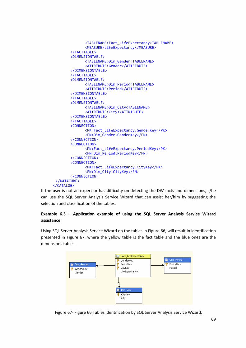
69
<TABLENAME>Fact_LifeExpectancy<TABLENAME> <MEASURE>LifeExpectancy</MEASURE>
</FACTTABLE> <DiMENSIONTABLE>
<TABLENAME>Dim_Gender<TABLENAME> <ATTRIBUTE>Gender</ATTRIBUTE>
</DIMENSIONTABLE> </FACTTABLE> <DiMENSIONTABLE>
<TABLENAME>Dim_Period<TABLENAME> <ATTRIBUTE>Period</ATTRIBUTE>
</DIMENSIONTABLE> </FACTTABLE> <DiMENSIONTABLE>
<TABLENAME>Dim_City<TABLENAME> <ATTRIBUTE>City</ATTRIBUTE>
</DIMENSIONTABLE> </FACTTABLE> <CONNECTION>
<PK>Fact_LifeExpectancy.GenderKey</PK> <FN>Dim_Gender.GenderKey</FN>
</CONNECTION> <CONNECTION>
<PK>Fact_LifeExpectancy.PeriodKey</PK> <FN>Dim_Period.PeriodKey</FN>
</CONNECTION> <CONNECTION>
<PK>Fact_LifeExpectancy.CityKey</PK> <FN>Dim_City.CityKey</FN>
</CONNECTION> </DATACUBE>
</CATALOG>
If the user is not an expert or has difficulty on detecting the DW facts and dimensions, s/he
can use the SQL Server Analysis Service Wizard that can assist her/him by suggesting the
selection and classification of the tables.
Example 6.3 – Application example of using the SQL Server Analysis Service Wizard
assistance
Using SQL Server Analysis Service Wizard on the tables in Figure 66, will result in identification
presented in Figure 67, where the yellow table is the fact table and the blue ones are the
dimensions tables.
Figure 67- Figure 66 Tables identification by SQL Server Analysis Service Wizard.
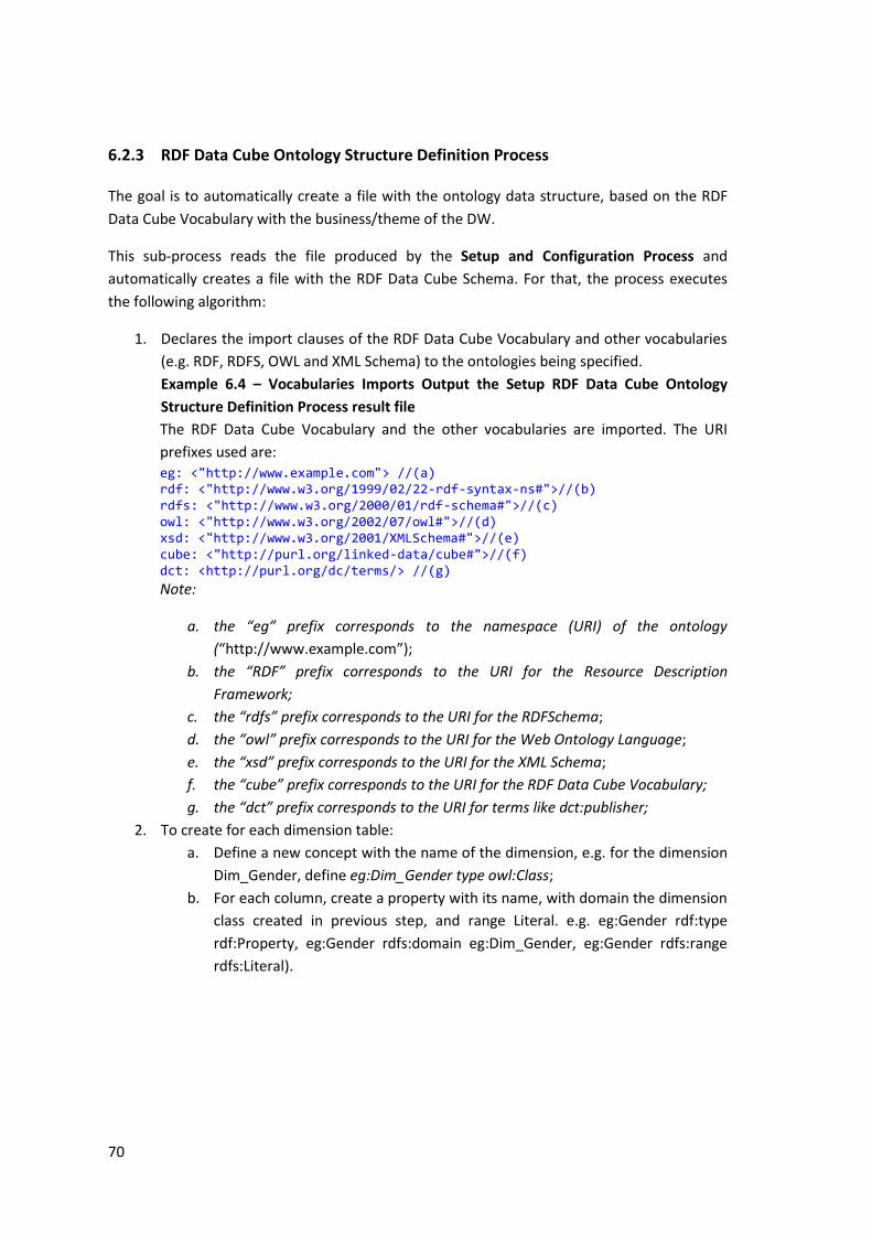
70
6.2.3 RDF Data Cube Ontology Structure Definition Process
The goal is to automatically create a file with the ontology data structure, based on the RDF
Data Cube Vocabulary with the business/theme of the DW.
This sub-process reads the file produced by the Setup and Configuration Process and
automatically creates a file with the RDF Data Cube Schema. For that, the process executes
the following algorithm:
1. Declares the import clauses of the RDF Data Cube Vocabulary and other vocabularies
(e.g. RDF, RDFS, OWL and XML Schema) to the ontologies being specified.
Example 6.4 – Vocabularies Imports Output the Setup RDF Data Cube Ontology
Structure Definition Process result file
The RDF Data Cube Vocabulary and the other vocabularies are imported. The URI
prefixes used are:
eg: <"http://www.example.com"> //(a) rdf: <"http://www.w3.org/1999/02/22-rdf-syntax-ns#">//(b) rdfs: <"http://www.w3.org/2000/01/rdf-schema#">//(c) owl: <"http://www.w3.org/2002/07/owl#">//(d) xsd: <"http://www.w3.org/2001/XMLSchema#">//(e) cube: <"http://purl.org/linked-data/cube#">//(f) dct: <http://purl.org/dc/terms/> //(g)
Note:
a. the “eg” prefix corresponds to the namespace (URI) of the ontology
(“http://www.example.com”);
b. the “RDF” prefix corresponds to the URI for the Resource Description
Framework;
c. the “rdfs” prefix corresponds to the URI for the RDFSchema;
d. the “owl” prefix corresponds to the URI for the Web Ontology Language;
e. the “xsd” prefix corresponds to the URI for the XML Schema;
f. the “cube” prefix corresponds to the URI for the RDF Data Cube Vocabulary;
g. the “dct” prefix corresponds to the URI for terms like dct:publisher;
2. To create for each dimension table:
a. Define a new concept with the name of the dimension, e.g. for the dimension
Dim_Gender, define eg:Dim_Gender type owl:Class;
b. For each column, create a property with its name, with domain the dimension
class created in previous step, and range Literal. e.g. eg:Gender rdf:type
rdf:Property, eg:Gender rdfs:domain eg:Dim_Gender, eg:Gender rdfs:range
rdfs:Literal).
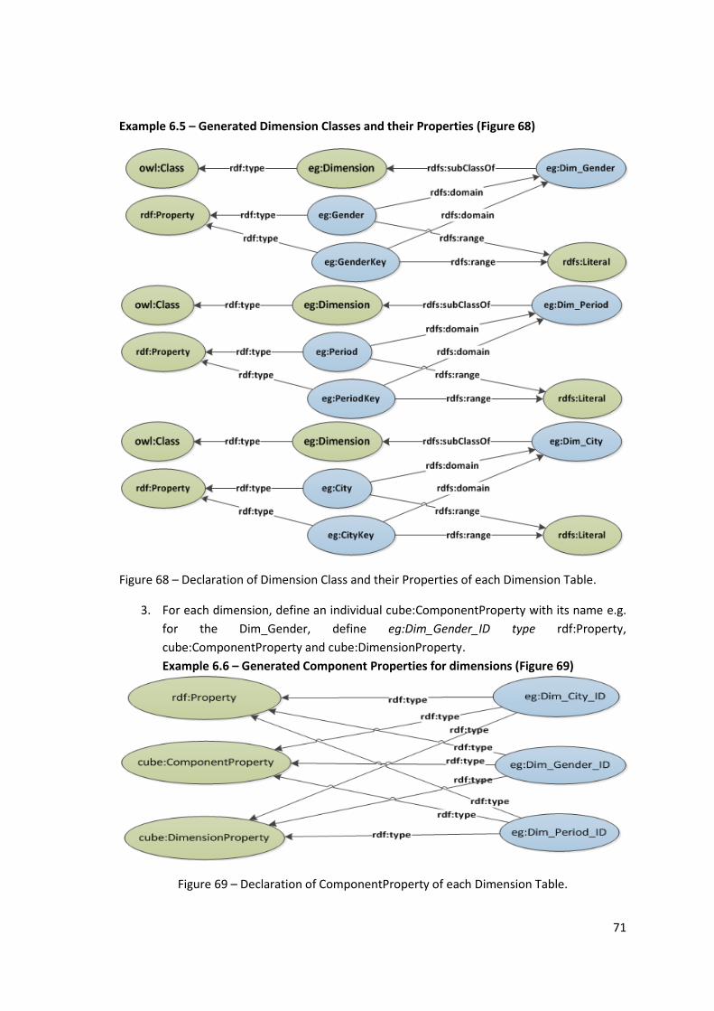
71
Example 6.5 – Generated Dimension Classes and their Properties (Figure 68)
Figure 68 – Declaration of Dimension Class and their Properties of each Dimension Table.
3. For each dimension, define an individual cube:ComponentProperty with its name e.g.
for the Dim_Gender, define eg:Dim_Gender_ID type rdf:Property,
cube:ComponentProperty and cube:DimensionProperty.
Example 6.6 – Generated Component Properties for dimensions (Figure 69)
Figure 69 – Declaration of ComponentProperty of each Dimension Table.
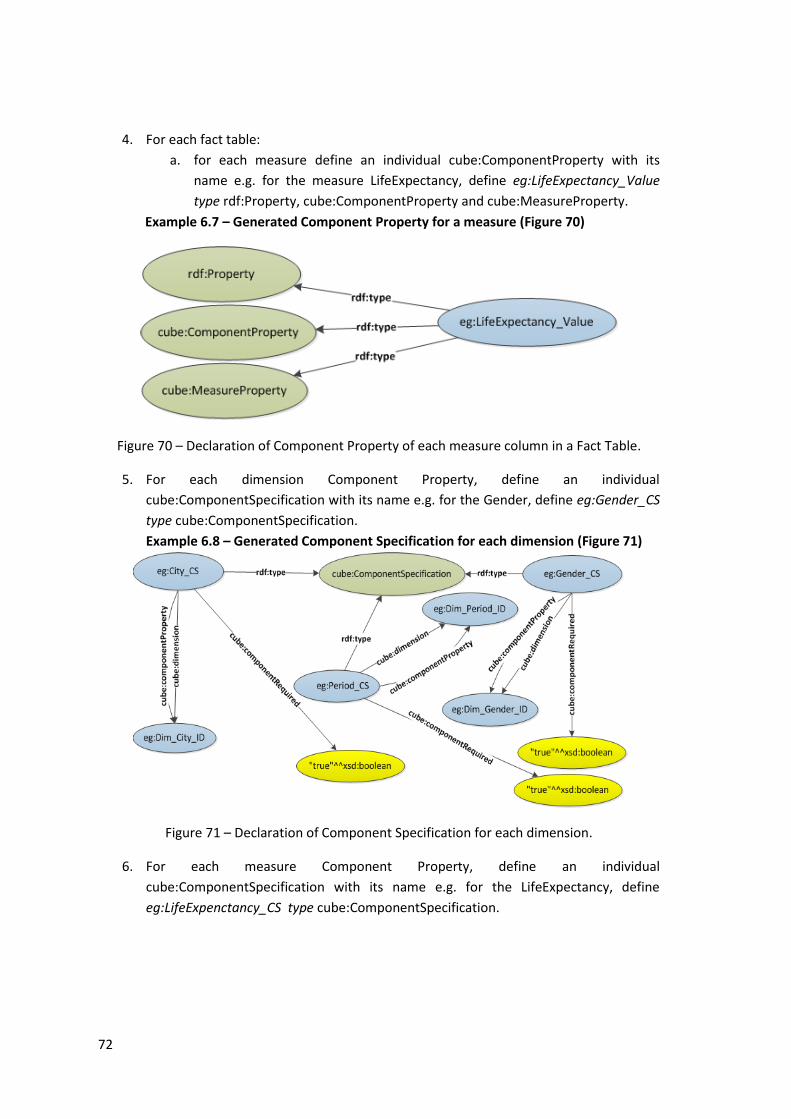
72
4. For each fact table:
a. for each measure define an individual cube:ComponentProperty with its
name e.g. for the measure LifeExpectancy, define eg:LifeExpectancy_Value
type rdf:Property, cube:ComponentProperty and cube:MeasureProperty.
Example 6.7 – Generated Component Property for a measure (Figure 70)
Figure 70 – Declaration of Component Property of each measure column in a Fact Table.
5. For each dimension Component Property, define an individual
cube:ComponentSpecification with its name e.g. for the Gender, define eg:Gender_CS
type cube:ComponentSpecification.
Example 6.8 – Generated Component Specification for each dimension (Figure 71)
Figure 71 – Declaration of Component Specification for each dimension.
6. For each measure Component Property, define an individual
cube:ComponentSpecification with its name e.g. for the LifeExpectancy, define
eg:LifeExpenctancy_CS type cube:ComponentSpecification.
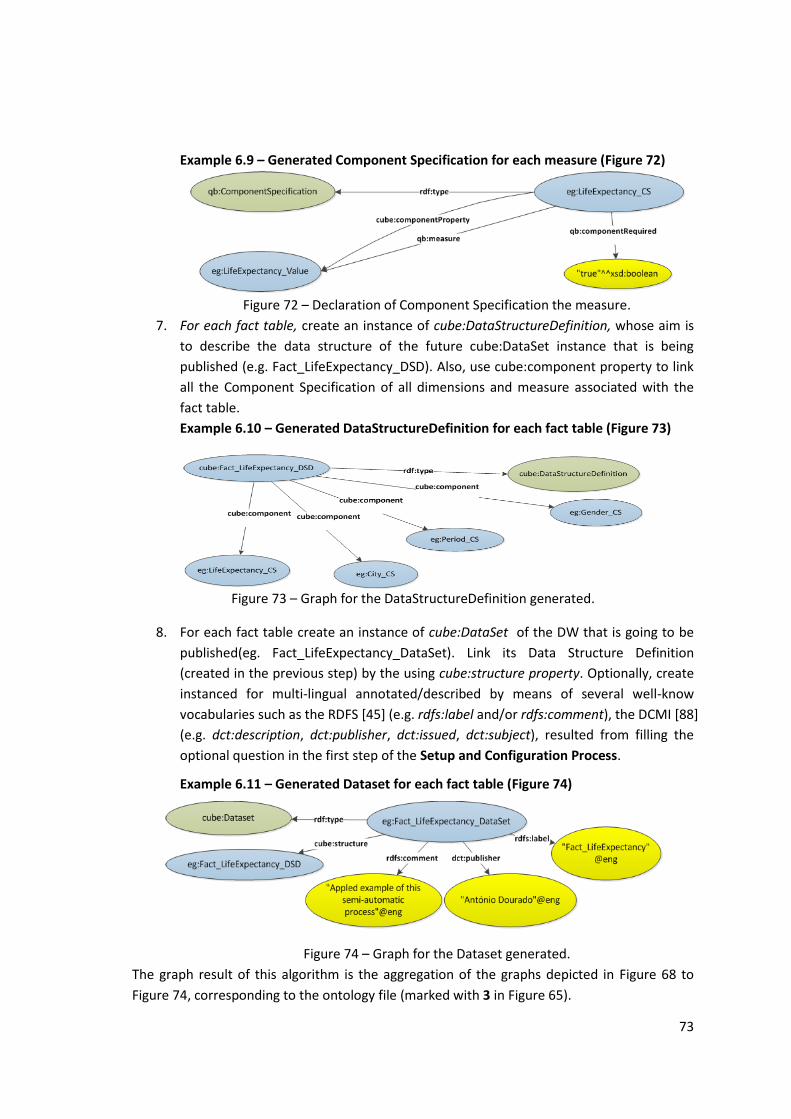
73
Example 6.9 – Generated Component Specification for each measure (Figure 72)
Figure 72 – Declaration of Component Specification the measure.
7. For each fact table, create an instance of cube:DataStructureDefinition, whose aim is
to describe the data structure of the future cube:DataSet instance that is being
published (e.g. Fact_LifeExpectancy_DSD). Also, use cube:component property to link
all the Component Specification of all dimensions and measure associated with the
fact table.
Example 6.10 – Generated DataStructureDefinition for each fact table (Figure 73)
Figure 73 – Graph for the DataStructureDefinition generated.
8. For each fact table create an instance of cube:DataSet of the DW that is going to be
published(eg. Fact_LifeExpectancy_DataSet). Link its Data Structure Definition
(created in the previous step) by the using cube:structure property. Optionally, create
instanced for multi-lingual annotated/described by means of several well-know
vocabularies such as the RDFS [45] (e.g. rdfs:label and/or rdfs:comment), the DCMI [88]
(e.g. dct:description, dct:publisher, dct:issued, dct:subject), resulted from filling the
optional question in the first step of the Setup and Configuration Process.
Example 6.11 – Generated Dataset for each fact table (Figure 74)
Figure 74 – Graph for the Dataset generated.
The graph result of this algorithm is the aggregation of the graphs depicted in Figure 68 to
Figure 74, corresponding to the ontology file (marked with 3 in Figure 65).
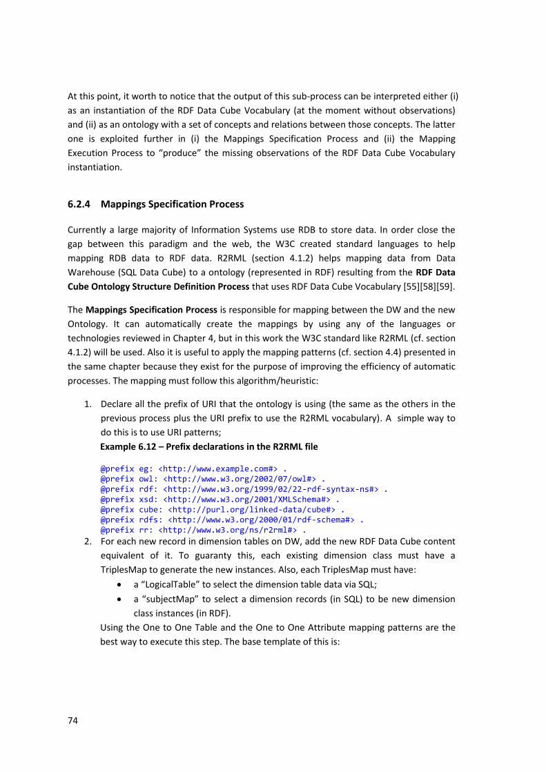
74
At this point, it worth to notice that the output of this sub-process can be interpreted either (i)
as an instantiation of the RDF Data Cube Vocabulary (at the moment without observations)
and (ii) as an ontology with a set of concepts and relations between those concepts. The latter
one is exploited further in (i) the Mappings Specification Process and (ii) the Mapping
Execution Process to “produce” the missing observations of the RDF Data Cube Vocabulary
instantiation.
6.2.4 Mappings Specification Process
Currently a large majority of Information Systems use RDB to store data. In order close the
gap between this paradigm and the web, the W3C created standard languages to help
mapping RDB data to RDF data. R2RML (section 4.1.2) helps mapping data from Data
Warehouse (SQL Data Cube) to a ontology (represented in RDF) resulting from the RDF Data
Cube Ontology Structure Definition Process that uses RDF Data Cube Vocabulary [55][58][59].
The Mappings Specification Process is responsible for mapping between the DW and the new
Ontology. It can automatically create the mappings by using any of the languages or
technologies reviewed in Chapter 4, but in this work the W3C standard like R2RML (cf. section
4.1.2) will be used. Also it is useful to apply the mapping patterns (cf. section 4.4) presented in
the same chapter because they exist for the purpose of improving the efficiency of automatic
processes. The mapping must follow this algorithm/heuristic:
1. Declare all the prefix of URI that the ontology is using (the same as the others in the
previous process plus the URI prefix to use the R2RML vocabulary). A simple way to
do this is to use URI patterns;
Example 6.12 – Prefix declarations in the R2RML file
@prefix eg: <http://www.example.com#> . @prefix owl: <http://www.w3.org/2002/07/owl#> . @prefix rdf: <http://www.w3.org/1999/02/22-rdf-syntax-ns#> . @prefix xsd: <http://www.w3.org/2001/XMLSchema#> . @prefix cube: <http://purl.org/linked-data/cube#> . @prefix rdfs: <http://www.w3.org/2000/01/rdf-schema#> . @prefix rr: <http://www.w3.org/ns/r2rml#> .
2. For each new record in dimension tables on DW, add the new RDF Data Cube content
equivalent of it. To guaranty this, each existing dimension class must have a
TriplesMap to generate the new instances. Also, each TriplesMap must have:
a “LogicalTable” to select the dimension table data via SQL;
a “subjectMap” to select a dimension records (in SQL) to be new dimension
class instances (in RDF).
Using the One to One Table and the One to One Attribute mapping patterns are the
best way to execute this step. The base template of this is:
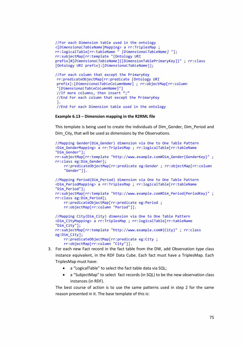
75
//For each Dimension table used in the ontology <[DimensionalTableName]Mapping> a rr:TriplesMap ; rr:logicalTable[rr:tableName " [DimensionalTableName] "]; rr:subjectMap[rr:template "[Ontology URI prefix]#[DimensionalTableName]{[DimensionTablePrimaryKey]}" ; rr:class [Ontology URI prefix]:[DimensionalTableName]]; //For each column that except the PrimaryKey rr:predicateObjectMap[rr:predicate [Ontology URI prefix]:[DimensionalTableColumnName] ; rr:objectMap[rr:column "[DimensionalTableColumnName]"] //If more columns, then insert “;” //End For each column that except the PrimaryKey ]. //End For each Dimension table used in the ontology
Example 6.13 – Dimension mapping in the R2RML file
This template is being used to create the individuals of Dim_Gender, Dim_Period and
Dim_City, that will be used as dimensions by the Observations.
//Mapping Gender(Dim_Gender) dimension via One to One Table Pattern <Dim_GenderMapping> a rr:TriplesMap ; rr:logicalTable[rr:tableName "Dim_Gender"]; rr:subjectMap[rr:template "http://www.example.com#Dim_Gender{GenderKey}" ; rr:class eg:Dim_Gender];
rr:predicateObjectMap[rr:predicate eg:Gender ; rr:objectMap[rr:column "Gender"]].
//Mapping Period(Dim_Period) dimension via One to One Table Pattern <Dim_PeriodMapping> a rr:TriplesMap ; rr:logicalTable[rr:tableName "Dim_Period"]; rr:subjectMap[rr:template "http://www.example.com#Dim_Period{PeriodKey}" ; rr:class eg:Dim_Period]; rr:predicateObjectMap[rr:predicate eg:Period ; rr:objectMap[rr:column "Period"]]. //Mapping City(Dim_City) dimension via One to One Table Pattern <Dim_CityMapping> a rr:TriplesMap ; rr:logicalTable[rr:tableName "Dim_City"]; rr:subjectMap[rr:template "http://www.example.com#{City}" ; rr:class eg:Dim_City]; rr:predicateObjectMap[rr:predicate eg:City ; rr:objectMap[rr:column "City"]].
3. For each new Fact record in the fact table from the DW, add Observation type class
instance equivalent, in the RDF Data Cube. Each fact must have a TriplesMap. Each
TriplesMap must have:
a “LogicalTable” to select the fact table data via SQL;
a “SubjectMap” to select fact records (in SQL) to be the new observation class
instances (in RDF).
The best course of action is to use the same patterns used in step 2 for the same
reason presented in it. The base template of this is:
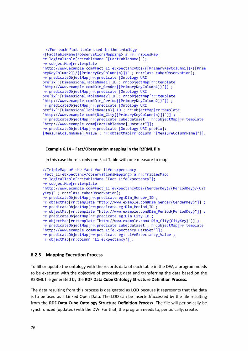
76
//For each Fact table used in the ontology <[FactTableName]/observationsMapping> a rr:TriplesMap; rr:logicalTable[rr:tableName "[FactTableName]"]; rr:subjectMap[rr:template "http://www.example.com#Fact_LifeExpectancyObs/{[PrimaryKeyColumn1]}/{[PrimaryKeyColumn2]}/{[PrimaryKeyColumn(n)]}" ; rr:class cube:Observation]; rr:predicateObjectMap[rr:predicate [Ontology URI prefix]:[DimensionalTableName1]_ID ; rr:objectMap[rr:template "http://www.example.com#Dim_Gender{[PrimaryKeyColumn1]}"]] ; rr:predicateObjectMap[rr:predicate [Ontology URI prefix]:[DimensionalTableName2]_ID ; rr:objectMap[rr:template "http://www.example.com#Dim_Period{[PrimaryKeyColumn2]}"]] ; rr:predicateObjectMap[rr:predicate [Ontology URI prefix]:[DimensionalTableName(n)]_ID ; rr:objectMap[rr:template "http://www.example.com#{Dim_City{[PrimaryKeyColumn(n)]}"]] ; rr:predicateObjectMap[rr:predicate cube:dataset ; rr:objectMap[rr:template "http://www.example.com#[FactTableName]_DataSet"]]; rr:predicateObjectMap[rr:predicate [Ontology URI prefix]: [MeasureColumnName]_Value ; rr:objectMap[rr:column "[MeasureColumnName]"]].
Example 6.14 – Fact/Observation mapping in the R2RML file
In this case there is only one Fact Table with one measure to map.
//TripleMap of the fact for life expectancy <Fact_LifeExpectancy/observationsMapping> a rr:TriplesMap; rr:logicalTable[rr:tableName "Fact_LifeExpectancy"]; rr:subjectMap[rr:template "http://www.example.com#Fact_LifeExpectancyObs/{GenderKey}/{PeriodKey}/{CityKey}" ; rr:class cube:Observation]; rr:predicateObjectMap[rr:predicate eg:Dim_Gender_ID ; rr:objectMap[rr:template "http://www.example.com#Dim_Gender{GenderKey}"]] ; rr:predicateObjectMap[rr:predicate eg:Dim_Period_ID ; rr:objectMap[rr:template "http://www.example.com#Dim_Period{PeriodKey}"]] ; rr:predicateObjectMap[rr:predicate eg:Dim_City_ID ; rr:objectMap[rr:template "http://www.example.com# Dim_City{CityKey}"]] ; rr:predicateObjectMap[rr:predicate cube:dataset ; rr:objectMap[rr:template "http://www.example.com#Fact_LifeExpectancy_DataSet"]]; rr:predicateObjectMap[rr:predicate eg: LifeExpectancy_Value ; rr:objectMap[rr:column "LifeExpectancy"]].
6.2.5 Mapping Execution Process
To fill or update the ontology with the records data of each table in the DW, a program needs
to be executed with the objective of processing data and transferring the data based on the
R2RML file generated by the RDF Data Cube Ontology Structure Definition Process.
The data resulting from this process is designated as LOD because it represents that the data
is to be used as a Linked Open Data. The LOD can be inserted/accessed by the file resulting
from the RDF Data Cube Ontology Structure Definition Process. The file will periodically be
synchronized (updated) with the DW. For that, the program needs to, periodically, create:
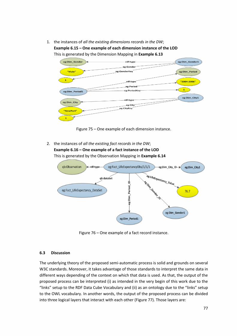
77
1. the instances of all the existing dimensions records in the DW;
Example 6.15 – One example of each dimension instance of the LOD
This is generated by the Dimension Mapping in Example 6.13
Figure 75 – One example of each dimension instance.
2. the instances of all the existing fact records in the DW;
Example 6.16 – One example of a fact instance of the LOD
This is generated by the Observation Mapping in Example 6.14
Figure 76 – One example of a fact record instance.
6.3 Discussion
The underlying theory of the proposed semi-automatic process is solid and grounds on several
W3C standards. Moreover, it takes advantage of those standards to interpret the same data in
different ways depending of the context on which that data is used. As that, the output of the
proposed process can be interpreted (i) as intended in the very begin of this work due to the
“links” setup to the RDF Data Cube Vocabulary and (ii) as an ontology due to the “links” setup
to the OWL vocabulary. In another words, the output of the proposed process can be divided
into three logical layers that interact with each other (Figure 77). Those layers are:
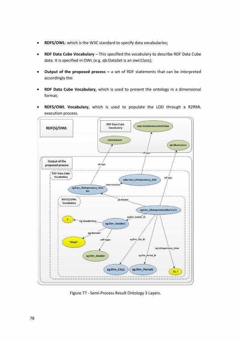
78
RDFS/OWL: which is the W3C standard to specify data vocabularies;
RDF Data Cube Vocabulary – This specified the vocabulary to describe RDF Data Cube
data. It is specified in OWL (e.g. qb:DataSet is an owl:Class);
Output of the proposed process – a set of RDF statements that can be interpreted
accordingly the:
RDF Data Cube Vocabulary, which is used to present the ontology in a dimensional
format;
RDFS/OWL Vocabulary, which is used to populate the LOD through a R2RML
execution process.
Figure 77 - Semi-Process Result Ontology 3 Layers.
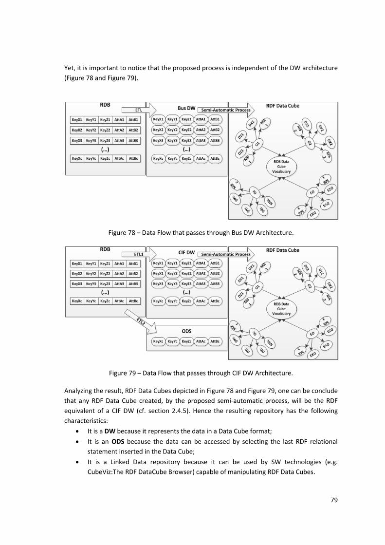
79
Yet, it is important to notice that the proposed process is independent of the DW architecture
(Figure 78 and Figure 79).
Figure 78 – Data Flow that passes through Bus DW Architecture.
Figure 79 – Data Flow that passes through CIF DW Architecture.
Analyzing the result, RDF Data Cubes depicted in Figure 78 and Figure 79, one can be conclude
that any RDF Data Cube created, by the proposed semi-automatic process, will be the RDF
equivalent of a CIF DW (cf. section 2.4.5). Hence the resulting repository has the following
characteristics:
It is a DW because it represents the data in a Data Cube format;
It is an ODS because the data can be accessed by selecting the last RDF relational
statement inserted in the Data Cube;
It is a Linked Data repository because it can be used by SW technologies (e.g.
CubeViz:The RDF DataCube Browser) capable of manipulating RDF Data Cubes.

80
81
7 Conclusions
The initial and primary emphasis of this work focuses on researching a simple and easy
process enabling to transform and/or expose the content of a Data Warehouse in RDF in order
to foster organizations (i) to have and promote better quality data (ii) to embrace and use
Semantic Web technologies and, therefore, (iii) to take advantages of that technology,
particularly in their Decision Support Systems.
As long as the research work evolved, it becomes clear that to achieve the intended goal it
was not necessary “to reinvent the wheel”. Instead, it was necessary to comprehend the full
potential of the already existing SW technologies such as the OWL, the RDF Data Cube and the
RDB to RDF Mapping standards and exploit/combine them together. The proposed process is
summarized in section 7.1.
The running example about the average life expectancy of people, by genders, by some
regions and by some periods of time was the only scenario used to demonstrate the
applicability and validity of the proposed process. Despite that, if more scenarios were used
that would just contribute on a matter of quantity (i.e. it would show the proposed process
works for one, two, or N DW scenarios). Due to the principles and ideas and technologies on
which the proposed process relies on quantity, is seen as a not relevant factor. On the other
hand, (more) experiments would enable us to found and systematize more indirect benefits to
organizations adopting the proposed process (cf. section 7.2).
7.1 The semi-automatic structure and elements
This section represents a summary of semi-automatic process elements and structure.
The structure is made of four sub-process elements. They are:
82
1. Setup and Configuration Process (section 6.2.2)
The user selects the fact tables and the dimension tables that s/he uses. Creates, as a
result, a file with processed data of the Data Warehouse used;
2. RDF Data Cube Ontology Structure Definition Process (section 6.2.3.)
Creates the RDF Data Cube ontology schema from the file produced by the Setup and
Configuration Process. Stores the ontology with the RDF Data Cube structure in a file.
3. Mappings Specification Process (section 6.2.4)
Creates a file with the R2RML mappings between the DW and the ontology file
created by RDF Data Cube Ontology Structure Definition Process.
4. Mapping Execution Process (section 6.2.5)
Periodically executes the R2RML Mapping file to create the LOD used by the ontology.
7.2 The Indirect benefits found
There are two main indirect benefits that the proposed semi-automatic process has:
1. Based on section 6.2, hypothetically, if a company has a Bus DW Architecture (cf.
section 2.4.4) and wants to change to CIF DW (more complete and complex than a Bus
DW) Architecture (cf. section 2.4.5), the best course of action is to use the semi-
automatic process, because:
a. It creates an Ontology with capabilities equivalent to a CIF DW;
b. it will be cheaper when migrating;
c. the data will be in a format that can be used by Semantic Web technologies;
2. Based on section 6.3, an application that executes this approach is capable of creating
ontologies that are capable of being used by DSS system (like Data Warehouses but in
a RDF format) and Semantic Web technologies.
7.3 Future Work and Open Issues
Mainly there needs to be the implementation of the semi-automatic process, but this
approach can be enhanced by:
Creating an alternative option in Setup and Configuration Process that lets the user
create a virtual DW directly from RDB. In other words, this new option would have a
ETL process integrate to it, like it shows on Figure 78 and Figure 79;
Giving Setup and Configuration Process more customizations, like:
o Selecting the dataset instance name;
o Manipulate connections between tables because some DW does not have the
tables connect by SQL structure statements. In the current state of this
approach, if the DW does not have connections between the DW tables, it will
not create the RDF Data Cube;
83
using the CubeViz:The RDF DataCube Browser that provides [89][90]:
o normal RDF queries using SPARQL;
o chart visualization of RDF Data Cube Components;
o a RDF Data Cube component selection interface that can:
select a Dataset;
Select a Slice;
Select a specific measure and attribute (the measure unit) property
encoded in the respective Dataset;
Select a set of dimension elements that are part of the dimensions
encoded in the respective Dataset;
Being able to create slices in a dataset by given the Mappings Specification Process
mapping that create links between the slices and the observations;
Being able to post the result RDF Data Cubes in existing public repositories, like
Sindece:The Semantic Web Index [91] and PublicData:Europe’s Public Data [92].
7.4 Closing Remarks
The DW example used on this document it is based on the example existing in the RDF Data
Cube Vocabulary (cf. chapters 5). It was chosen because it was a good and a more simple way
of exposing this knowledge.
The use of work does not invalidate a user that is accustomed to the Data Warehouse. That
user can still use the DW and learn little by little the mechanics and theories need to operate
the RDF Data Cube. This can evolve a Data Analyst [93] into a Semantic Data Analyst, which
one can assume that s/he has the same knowledge as a Data Analyst and as a person that has
some expertise in Linked Data.
Unfortunately this approach was not tested with real-world data. In fact, conducting
experiments with real-world data is one of the most relevant open issues of this work, which
might show deficiencies concerning the coverage of the rules and poor tool performance.

84
85
References
[1] Surajit Chaudhuri and Umeshwar Dayal, “An overview of data warehousing and
OLAP technology,” SIGMOD Rec., vol. 26, no. 1, pp. 65–74, 1997.
[2] Sean Kelly, Data Warehousing: The Route to Mass Customisation, 1st ed. New
York, NY, USA: John Wiley & Sons, Inc., 1994.
[3] H. P. Luhn, “A business intelligence system,” IBM Journal of Research and
Development, vol. 2, no. 4, pp. 314–319, 1958.
[4] “RDF - Semantic Web Standards.” [Online]. Available: http://www.w3.org/RDF/.
[Accessed: 26-Sep-2013].
[5] “Data - W3C.” [Online]. Available:
http://www.w3.org/standards/semanticweb/data. [Accessed: 12-Jun-2014].
[6] Christian Bizer, Tom Heath, and Tim Berners-Lee, “Linked Data - the story so
far,” International Journal on Semantic Web and Information Systems, vol. 5, no.
3, pp. 1–22, 2009.
[7] “Linked Data - Design Issues.” [Online]. Available:
http://www.w3.org/DesignIssues/LinkedData.html. [Accessed: 12-Jun-2014].
[8] “Frequently Asked Questions (FAQs) | Linked Data - Connect Distributed Data
across the Web.” [Online]. Available: http://linkeddata.org/faq. [Accessed: 12-
Jun-2014].
[9] Tim Berners-Lee, James Hendler, and Ora Lassila, “THE SEMANTIC WEB.,”
Scientific American, vol. 284, no. 5, p. 34, May 2001.
[10] “Semantic Web - W3C.” [Online]. Available:
http://www.w3.org/standards/semanticweb/. [Accessed: 26-Sep-2013].
[11] “RDF Vocabulary Description Language 1.0: RDF Schema.” [Online]. Available:
http://www.w3.org/TR/2004/REC-rdf-schema-20040210/. [Accessed: 06-Aug-
2014].
[12] “The RDF Data Cube Vocabulary.” [Online]. Available:
http://www.w3.org/TR/2014/REC-vocab-data-cube-20140116/. [Accessed: 20-
Mar-2014].
[13] “Operational Systems: Guide to Data Warehousing and Business Intelligence.”
[Online]. Available: http://data-warehouses.net/architecture/operational.html.
[Accessed: 04-Aug-2014].
86
[14] “OLAP vs OLTP: what makes the difference.” [Online]. Available:
http://www.cbsolution.net/techniques/ontarget/olap_vs_oltp_what_makes.
[Accessed: 13-Aug-2014].
[15] Edmund F. Codd, “A relational model of data for large shared data banks,”
Communications of the ACM, vol. 13, no. 6, pp. 377–387, 1970.
[16] “OLTP vs. OLAP.” [Online]. Available: http://datawarehouse4u.info/OLTP-vs-
OLAP.html. [Accessed: 04-Aug-2014].
[17] Preeti S. Patil, Srikantha Rao, and Suryakant B. Patil, “Optimization of Data
Warehousing System: Simplification in Reporting and Analysis,” IJCA
Proceedings on International Conference and workshop on Emerging Trends in
Technology (ICWET), no. 9, pp. 33–37, 2011.
[18] Shah J. Miah, Don Kerr, and Liisa von Hellens, “A collective artefact design of
decision support systems: design science research perspective,” Info Technology
& People, vol. 27, no. 3, pp. 259–279, Jul. 2014.
[19] Erik Thomsen, OLAP Solutions: Building Multidimensional Information Systems,
2nd ed. John Wiley and Sons, 2002.
[20] Ralph Kimball, The data warehouse toolkit: The definitive guide to dimensional
modeling, 3rd ed. Indianapolis, IN: John Wiley & Sons, 2013.
[21] William H. Inmon, Building the Data Warehouse, 4. Aufl. John Wiley & Sons,
2005.
[22] “CSE2DBF: Lecture 24 - Data Warehouse.” [Online]. Available:
http://ironbark.xtelco.com.au/subjects/DB/2010s2/lectures/lecture24.html.
[Accessed: 03-Jun-2014].
[23] “Data Warehouse Architecture.” [Online]. Available:
http://www.1keydata.com/datawarehousing/data-warehouse-architecture.html.
[Accessed: 12-Aug-2014].
[24] Claudia Imhoff, Nicholas Galemmo, and Jonathan G. Gege, “Mastering Data
Warehouse Design: Relational and Dimensional Techniques,” Wiley, 2003, pp. 3–
27; 383–396.
[25] Ralph Kimball, Laura Reeves, Margy Ross, and Warren Thornthwaite, “The Data
Warehouse Lifecycle Toolkit: Expert Methods for Designing, Developing, and
Deploying Data Warehouses,” Wiley, 1998, pp. 8.1–10.21.
[26] Jeffrey A. Hoffer, Mary B. Prescott, and Heikki Topi, “Modern Database
Management,” Pearson Education, 2008, pp. 499 – 556.
[27] Drew Cardon, “Database vs Data Warehouse: A Comparative Review.” [Online].
Available: http://www.healthcatalyst.com/database-vs-data-warehouse-a-
comparative-review.
[28] “Dimension Tables.” [Online]. Available: http://technet.microsoft.com/en-
us/library/aa905979(v=sql.80).aspx. [Accessed: 11-Jun-2014].
[29] “Dimensional schemas.” [Online]. Available:
http://pic.dhe.ibm.com/infocenter/dataarch/v9r1/index.jsp?topic=%2Fcom.ibm.dat
atools.dimensional.ui.doc%2Ftopics%2Fc_dm_dimschemas.html. [Accessed: 10-
Jun-2014].
[30] “Data Warehouse Schema Architecture - fact constellation schema.” [Online].
Available: http://datawarehouse4u.info/Data-warehouse-schema-architecture-fact-
constellation-schema.html. [Accessed: 10-Jun-2014].
87
[31] Wil M.P. van der Aalst, Process Cubes: Slicing, Dicing, Rolling Up and Drilling
Down Event Data for Process Mining. Asia Pacific conference on Business
Process Management, Beijing, China, 2013.
[32] Ralph Kimball and Joe Caserta, The Data Warehouse ETL Toolkit: Practical
Techniques for Extracting, Cleaning, Conforming, and Delivering Data, 1st ed.
Wiley, 2004.
[33] “CIF.” [Online]. Available: http://www.biosino.org/bioinformatics/011225-4.htm.
[Accessed: 15-Oct-2014].
[34] Vinton G. Cerf and Robert E. Icahn, “A protocol for packet network
intercommunication,” ACM SIGCOMM Computer Communication Review, vol.
35, no. 2, p. 71, Apr. 2005.
[35] Elwood N. Chapman, Attitude: Your Most Priceless Possession, 2nd ed. Los Altos,
CA: Crisp Publications, 1990.
[36] J. Richard Eiser, Social Psychology: Attitudes, Cognition, and Social Behaviour,
2nd ed. New York: Cambridge University Press, 1986.
[37] Krzysztof Janowicz, Pascal Hitzler, Benjamin Adams, Dave Kolas, and Charles
Vardeman, “Five Stars of Linked Data Vocabulary Use.” [Online]. Available:
http://www.semantic-web-journal.net/content/five-stars-linked-data-vocabulary-
use.
[38] “LOD cloud diagram.” [Online]. Available: http://lod-cloud.net/versions/2011-09-
19/lod-cloud.html. [Accessed: 15-Jun-2014].
[39] Christian Bizer, Jens Lehmann, Georgi Kobilarov, Sören Auer, Christian Becker,
Richard Cyganiak, and Sebastian Hellmann, “DBpedia - A crystallization point
for the Web of Data,” Web Semantics: Science, Services and Agents on the World
Wide Web, vol. 7, no. 3, pp. 154–165, Sep. 2009.
[40] “GeoNames.” [Online]. Available: http://www.geonames.org/. [Accessed: 15-Jun-
2014].
[41] “FOAF (2000-2014+).” [Online]. Available: http://www.foaf-project.org/.
[Accessed: 15-Jun-2014].
[42] Charles L. Griswold, “Recollection Dialectic and Ontology Kenn,” in Platonic
Writings/Platonic Readings, Penn State Press, p. 237.
[43] Nicola Guarino, Daniel Oberle, and Steffen Staab, “What Is an Ontology?,” in
Handbook on Ontologies, Steffen Staab and Ruid Studer, Eds. Springer Berlin
Heidelberg, 2009, pp. 1–17.
[44] A. Maedche and Steffen Staab, “Ontology learning for the Semantic Web,” IEEE
Intell. Syst., vol. 16, no. 2, pp. 72–79, Mar. 2001.
[45] “RDF Schema 1.1.” [Online]. Available: http://www.w3.org/TR/rdf-schema/.
[Accessed: 22-Jul-2014].
[46] “Media Types Issues for Text RDF Formats,” Jan-2008. [Online]. Available:
http://www.w3.org/2008/01/rdf-media-types. [Accessed: 04-Aug-2014].
[47] “RDF Graph and Syntax - Introduction to ontologies and semantic web - tutorial.”
[Online]. Available: http://www.obitko.com/tutorials/ontologies-semantic-
web/rdf-graph-and-syntax.html. [Accessed: 24-Sep-2013].
[48] “OWL Web Ontology Language Overview.” [Online]. Available:
http://www.w3.org/TR/owl-features/. [Accessed: 25-Aug-2014].
[49] “OWL 2 Web Ontology Language Profiles (Second Edition).” [Online]. Available:
http://www.w3.org/TR/owl2-profiles/. [Accessed: 24-Sep-2014].
88
[50] John Hebeler, Matthew Fisher, Ryan Blace, and Andrew Perez-Lopez,
Programming the Semantic Web. Indianapolis IN: John Wiley & Sons, 2009.
[51] “SPARQL 1.1 Query Language.” [Online]. Available:
http://www.w3.org/TR/sparql11-query/. [Accessed: 31-Mar-2014].
[52] “Benefits - Library Linked Data.” [Online]. Available:
http://www.w3.org/2005/Incubator/lld/wiki/Benefits. [Accessed: 26-Sep-2014].
[53] “Relational Databases and the Semantic Web (in Design Issues).” [Online].
Available: http://www.w3.org/DesignIssues/RDB-RDF.html. [Accessed: 22-Sep-
2013].
[54] “Use Cases and Requirements for Mapping Relational Databases to RDF.”
[Online]. Available: http://www.w3.org/TR/rdb2rdf-ucr/#intro. [Accessed: 16-
Oct-2013].
[55] Chang-Joo Moon, Mi-Young Choi, Doo-Kwon Baik, Young-Jun Wie, and Joong-
Hee Park, “Interoperability between a Relational Data Model and an RDF Data
Model,” in Networked Computing and Advanced Information Management
(NCM), 2010 Sixth International Conference, Seoul: IEEE, 2010, pp. 335 – 340.
[56] Kurt Rohloff, Mike Dean, Ian Emmons, Dorene Ryde, and John Sumner, “An
evaluation of triple-store technologies for large data stores,” in Proceedings of the
2007 OTM Confederated international conference on On the move to meaningful
internet systems-Volume Part II, Vilamoura, Portugal, 2007, pp. 1105–1114.
[57] “W3C RDB2RDF Working Group.” [Online]. Available:
http://www.w3.org/2001/sw/rdb2rdf/. [Accessed: 24-Sep-2013].
[58] “A Direct Mapping of Relational Data to RDF.” [Online]. Available:
http://www.w3.org/TR/rdb-direct-mapping/. [Accessed: 25-Sep-2013].
[59] “R2RML: RDB to RDF Mapping Language.” [Online]. Available:
http://www.w3.org/2001/sw/rdb2rdf/r2rml/. [Accessed: 30-Sep-2013].
[60] Alan Beaulieu, “Learning SQL,” in Learning SQL, 2nd ed., O’Reilly Media, 2009,
pp. 75–77; 159–163.
[61] Matthias Hert, Gerald Reif, and Harald C. Gall, “A comparison of RDB-to-RDF
mapping languages,” Proceedings of the 7th International Conference on
Semantic Systems, pp. 25–32, 2011.
[62] Wondu Y. Mallede, Farhi Marir, and Vassil T. Vassilev, “Algorithms for
Mapping RDB Schema to RDF for Facilitating Access to Deep Web,” in WEB
2013, The First International Conference on Building and Exploring Web Based
Environments, Seville, Spain: IARIA, 2013, pp. 32–41.
[63] Jesús Barrasa, Oscar Corcho, and Asunción Gómez-Pérez, “Fund Finder: A case
study of database-to-ontology mapping,” in Proceedings of the Semantic
Integration Workshop, Sanibel Island, Florida, USA: ISWC, 2003.
[64] Jesús Barrasa, Óscar Corcho, and Asunción Gómez-Pérez, “R2O, an Extensible
and Semantically Based Database- to-ontology Mapping Language,” in
Proceedings of the Second Workshop on Semantic Web and Databases (SWDB
2004), vol. 3372, Toronto, Canada: Springer-Verlag, 2004, pp. 1069–1070.
[65] Cristian Pérez de Labor and Stefan Conrad, “Relational.OWL - A Data and
Schema Representation Format Based on OWL,” in Proceedings of the 2Nd Asia-
Pacific Conference on Conceptual Modelling, vol. 43, Newcastle, New South
Wales, Australia: Australian Computer Society, Inc., 2005, pp. 89–96.
[66] “Virtuoso Open-Source Wiki : Mapping SQL Data to Linked Data Views.”
[Online]. Available:

89
http://www.openlinksw.com/dataspace/doc/dav/wiki/Main/VOSSQL2RDF.
[Accessed: 19-Oct-2013].
[67] Richard Cyganiak, Chris Bizer, Jörg Garbers, Oliver Maresch, and Christian
Becker, “The D2RQ Mapping Language | The D2RQ Platform.” [Online].
Available: http://d2rq.org/d2rq-language. [Accessed: 04-Nov-2013].
[68] “triplify.org : Overview.” [Online]. Available: http://triplify.org/Overview.
[Accessed: 19-Oct-2013].
[69] Matthias Hert, Gerald Reif, and Harald C. Gall, “Updating Relational Data via
SPARQL/Update,” in Proceedings of the 2010 EDBT/ICDT Workshops, Lausanne,
Switzerland: ACM, 2010, pp. 24:1–24:8.
[70] Juan F. Sequeda and Daniel P. Miranker, “Ultrawrap: SPARQL Execution on
Relational Data,” Web Semantics: Science, Services and Agents on the World
Wide Web, vol. 22, 2013.
[71] “Ultrawrap - Semantic Web Standards.” [Online]. Available:
https://www.w3.org/2001/sw/wiki/Ultrawrap. [Accessed: 17-Feb-2014].
[72] “-ontop-.” [Online]. Available: http://ontop.inf.unibz.it/. [Accessed: 29-Jan-2014].
[73] Wondu Y. Mallede, Farhi Marir, and Vassil T. Vassilev, “Algorithms for
Mapping RDB Schema to RDF for Facilitating Access to Deep Web.” [Online].
Available:
http://www.thinkmind.org/index.php?view=article&articleid=web_2013_2_30_40
075. [Accessed: 17-Oct-2013].
[74] Roy Fielding, “Relative Uniform Resource Locators,” Jun-1995. [Online].
Available: http://www.rfc-editor.org/rfc/rfc1808.txt. [Accessed: 14-Dec-2013].
[75] “Identifier Design Patterns.” [Online]. Available:
http://www.cambridgesemantics.com/semantic-university/identifier-design-
patterns. [Accessed: 14-Dec-2013].
[76] Juan Sequeda, Freddy Priyatna, and Boris Villazón-Terrazas, “Relational
Database to RDF Mapping Patterns,” in Workshop on Ontology Patterns
(WOP2012), Boston, USA, 2012.
[77] “A Practical Guide To Building OWL Ontologies Using Prot_eg_e 4 and CO-
ODE Tools Edition 1.3.” [Online]. Available:
http://130.88.198.11/tutorials/protegeowltutorial/. [Accessed: 12-Nov-2013].
[78] Robert Stevens and Uli Sattler, “Disjointness Between Classes in an Ontology |
Ontogenesis.” [Online]. Available: http://ontogenesis.knowledgeblog.org/1260.
[Accessed: 11-Dec-2013].
[79] T. le Dinh and G. Fillion, “Acquiring Domain Knowledge of Information Systems:
The Information System upon Information Systems Approach,” in Academy of
Information and Management Sciences Journal, Allied Academies, 2007, p. 22.
[80] “Oracle Semantic Technologies Overview.” [Online]. Available:
http://docs.oracle.com/cd/B28359_01/appdev.111/b28397/sdo_rdf_concepts.htm#
RDFRM562. [Accessed: 17-Oct-2014].
[81] “Rdb2RdfXG/StateOfTheArt - W3C Wiki.” [Online]. Available:
http://www.w3.org/wiki/Rdb2RdfXG/StateOfTheArt#Tools.2FApplications.
[Accessed: 12-Dec-2013].
[82] Sören Auer, Sebastian Dietzold, Jens Lehmann, Sebastian Hellmann, and David
Aumueller, “Triplify – Light-Weight Linked Data Publication from Relational
Databases,” in Proceedings of the 18th International Conference on World Wide
Web, Madrid, Spain: ACM, 2009, pp. 621–630.
90
[83] Kingsley Idehen, “Virtuoso RDF Views over RDBMS Data Sources -- Part 1 -
YouTube.” [Online]. Available: http://www.youtube.com/watch?v=bj7AbJ0ZYCk.
[Accessed: 27-Jan-2014].
[84] Kingsley Idehen, “Virtuoso RDF Views over RDBMS Data Sources -- Part 2 -
YouTube.” [Online]. Available: http://www.youtube.com/watch?v=yXNlcISS0aY.
[Accessed: 27-Jan-2014].
[85] “The D2RQ Platform – Accessing Relational Databases as Virtual RDF Graphs.”
[Online]. Available: http://d2rq.org/. [Accessed: 27-Jan-2014].
[86] “SKOS - Semantic Web Standards,” 18-Aug-2009. [Online]. Available:
http://www.w3.org/2001/sw/wiki/SKOS. [Accessed: 22-Oct-2014].
[87] “SDMX – Statistical Data and Metadata Exchange.” [Online]. Available:
http://sdmx.org/. [Accessed: 22-Oct-2014].
[88] “DCMI Abstract Model,” 04-Jun-2007. [Online]. Available:
http://dublincore.org/documents/abstract-model/. [Accessed: 22-Jul-2014].
[89] “CubeViz — Agile Knowledge Engineering and Semantic Web (AKSW).”
[Online]. Available: http://aksw.org/Projects/CubeViz.html. [Accessed: 02-Oct-
2014].
[90] “European Commision - Open Data Portal — Welcome to OntoWiki.” [Online].
Available: http://open-data.europa.eu/cubeviz/. [Accessed: 02-Oct-2014].
[91] “Sindice - The semantic web index.” [Online]. Available: http://sindice.com/.
[Accessed: 02-Oct-2014].
[92] “Welcome - PublicData.eu.” [Online]. Available: http://publicdata.eu/. [Accessed:
02-Oct-2014].
[93] “The Data Analyst Job Description : Data Analysts Online Training.” [Online].
Available: http://www.dataanalystbootcamp.com/the-data-analyst-job-description/.
[Accessed: 26-Oct-2014].
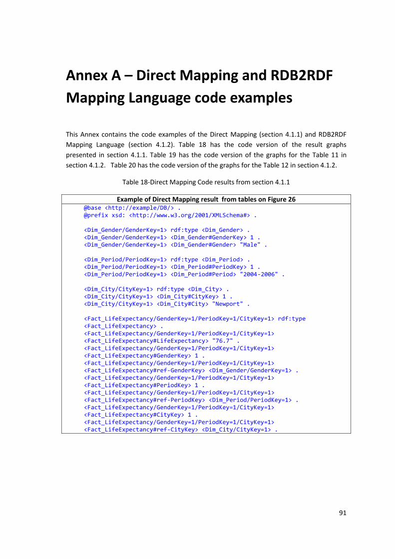
91
Annex A – Direct Mapping and RDB2RDF
Mapping Language code examples
This Annex contains the code examples of the Direct Mapping (section 4.1.1) and RDB2RDF
Mapping Language (section 4.1.2). Table 18 has the code version of the result graphs
presented in section 4.1.1. Table 19 has the code version of the graphs for the Table 11 in
section 4.1.2. Table 20 has the code version of the graphs for the Table 12 in section 4.1.2.
Table 18-Direct Mapping Code results from section 4.1.1
Example of Direct Mapping result from tables on Figure 26 @base <http://example/DB/> . @prefix xsd: <http://www.w3.org/2001/XMLSchema#> . <Dim_Gender/GenderKey=1> rdf:type <Dim_Gender> . <Dim_Gender/GenderKey=1> <Dim_Gender#GenderKey> 1 . <Dim_Gender/GenderKey=1> <Dim_Gender#Gender> "Male" . <Dim_Period/PeriodKey=1> rdf:type <Dim_Period> . <Dim_Period/PeriodKey=1> <Dim_Period#PeriodKey> 1 . <Dim_Period/PeriodKey=1> <Dim_Period#Period> "2004-2006" . <Dim_City/CityKey=1> rdf:type <Dim_City> . <Dim_City/CityKey=1> <Dim_City#CityKey> 1 . <Dim_City/CityKey=1> <Dim_City#City> "Newport" . <Fact_LifeExpectancy/GenderKey=1/PeriodKey=1/CityKey=1> rdf:type <Fact_LifeExpectancy> . <Fact_LifeExpectancy/GenderKey=1/PeriodKey=1/CityKey=1> <Fact_LifeExpectancy#LifeExpectancy> "76.7" . <Fact_LifeExpectancy/GenderKey=1/PeriodKey=1/CityKey=1> <Fact_LifeExpectancy#GenderKey> 1 . <Fact_LifeExpectancy/GenderKey=1/PeriodKey=1/CityKey=1> <Fact_LifeExpectancy#ref-GenderKey> <Dim_Gender/GenderKey=1> . <Fact_LifeExpectancy/GenderKey=1/PeriodKey=1/CityKey=1> <Fact_LifeExpectancy#PeriodKey> 1 . <Fact_LifeExpectancy/GenderKey=1/PeriodKey=1/CityKey=1> <Fact_LifeExpectancy#ref-PeriodKey> <Dim_Period/PeriodKey=1> . <Fact_LifeExpectancy/GenderKey=1/PeriodKey=1/CityKey=1> <Fact_LifeExpectancy#CityKey> 1 . <Fact_LifeExpectancy/GenderKey=1/PeriodKey=1/CityKey=1> <Fact_LifeExpectancy#ref-CityKey> <Dim_City/CityKey=1> .
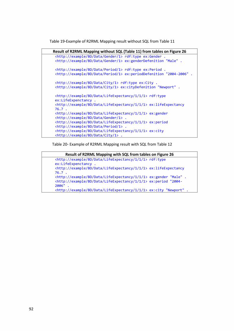
92
Table 19-Example of R2RML Mapping result without SQL from Table 11
Result of R2RML Mapping without SQL (Table 11) from tables on Figure 26 <http://example/BD/Data/Gender/1> rdf:type ex:Gender . <http://example/BD/Data/Gender/1> ex:genderDefenition "Male" . <http://example/BD/Data/Period/1> rdf:type ex:Period . <http://example/BD/Data/Period/1> ex:periodDefenition "2004-2006" . <http://example/BD/Data/City/1> rdf:type ex:City . <http://example/BD/Data/City/1> ex:cityDefenition "Newport" . <http://example/BD/Data/LifeExpectancy/1/1/1> rdf:type ex:LifeExpenctancy . <http://example/BD/Data/LifeExpectancy/1/1/1> ex:lifeExpectancy 76.7 . <http://example/BD/Data/LifeExpectancy/1/1/1> ex:gender <http://example/BD/Data/Gender/1> . <http://example/BD/Data/LifeExpectancy/1/1/1> ex:period <http://example/BD/Data/Period/1> . <http://example/BD/Data/LifeExpectancy/1/1/1> ex:city <http://example/BD/Data/City/1> .
Table 20- Example of R2RML Mapping result with SQL from Table 12
Result of R2RML Mapping with SQL from tables on Figure 26 <http://example/BD/Data/LifeExpectancy/1/1/1> rdf:type ex:LifeExpenctancy . <http://example/BD/Data/LifeExpectancy/1/1/1> ex:lifeExpectancy 76.7 . <http://example/BD/Data/LifeExpectancy/1/1/1> ex:gender "Male" . <http://example/BD/Data/LifeExpectancy/1/1/1> ex:period "2004-2006" . <http://example/BD/Data/LifeExpectancy/1/1/1> ex:city "Newport" .
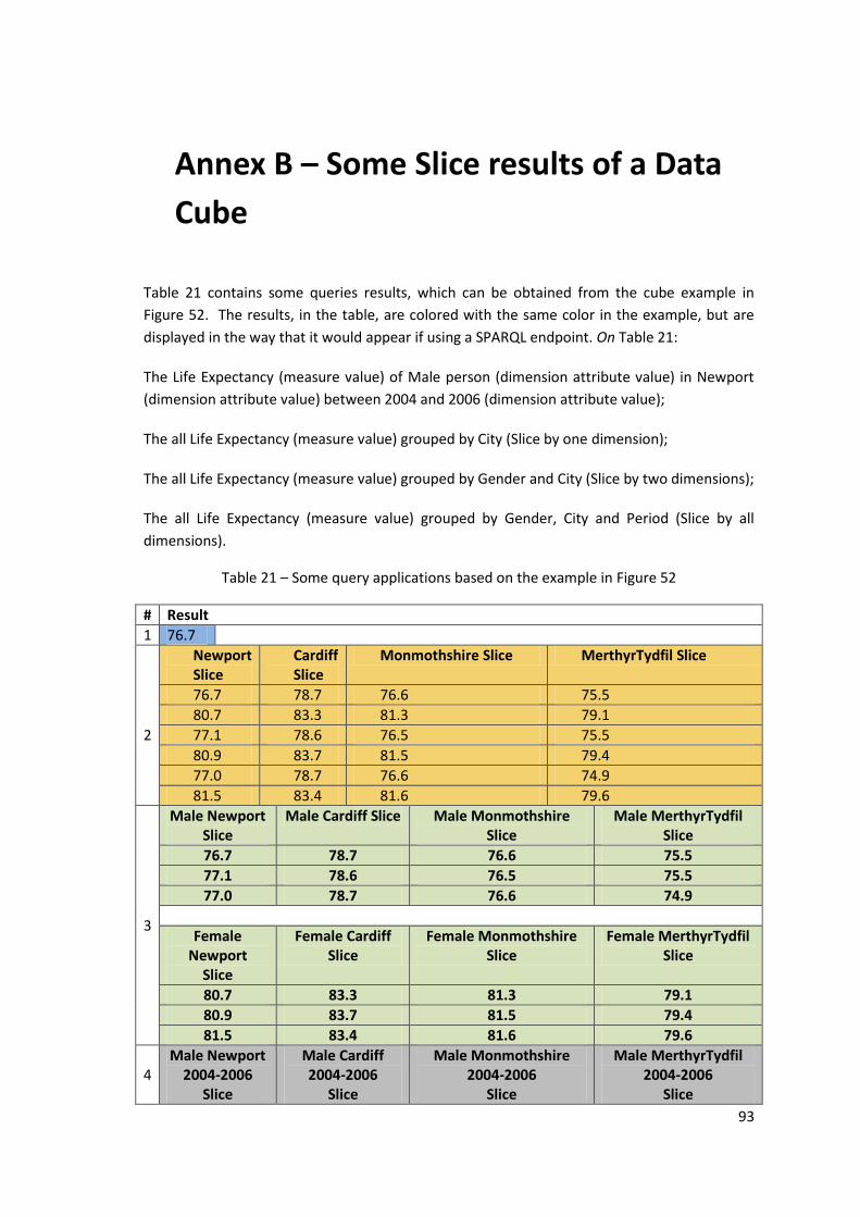
93
Annex B – Some Slice results of a Data
Cube
Table 21 contains some queries results, which can be obtained from the cube example in
Figure 52. The results, in the table, are colored with the same color in the example, but are
displayed in the way that it would appear if using a SPARQL endpoint. On Table 21:
The Life Expectancy (measure value) of Male person (dimension attribute value) in Newport
(dimension attribute value) between 2004 and 2006 (dimension attribute value);
The all Life Expectancy (measure value) grouped by City (Slice by one dimension);
The all Life Expectancy (measure value) grouped by Gender and City (Slice by two dimensions);
The all Life Expectancy (measure value) grouped by Gender, City and Period (Slice by all
dimensions).
Table 21 – Some query applications based on the example in Figure 52
# Result
1 76.7
2
Newport Slice
Cardiff Slice
Monmothshire Slice MerthyrTydfil Slice
76.7 78.7 76.6 75.5
80.7 83.3 81.3 79.1
77.1 78.6 76.5 75.5
80.9 83.7 81.5 79.4
77.0 78.7 76.6 74.9
81.5 83.4 81.6 79.6
3
Male Newport Slice
Male Cardiff Slice Male Monmothshire Slice
Male MerthyrTydfil Slice
76.7 78.7 76.6 75.5
77.1 78.6 76.5 75.5
77.0 78.7 76.6 74.9
Female Newport
Slice
Female Cardiff Slice
Female Monmothshire Slice
Female MerthyrTydfil Slice
80.7 83.3 81.3 79.1
80.9 83.7 81.5 79.4
81.5 83.4 81.6 79.6
4 Male Newport
2004-2006 Slice
Male Cardiff 2004-2006
Slice
Male Monmothshire 2004-2006
Slice
Male MerthyrTydfil 2004-2006
Slice
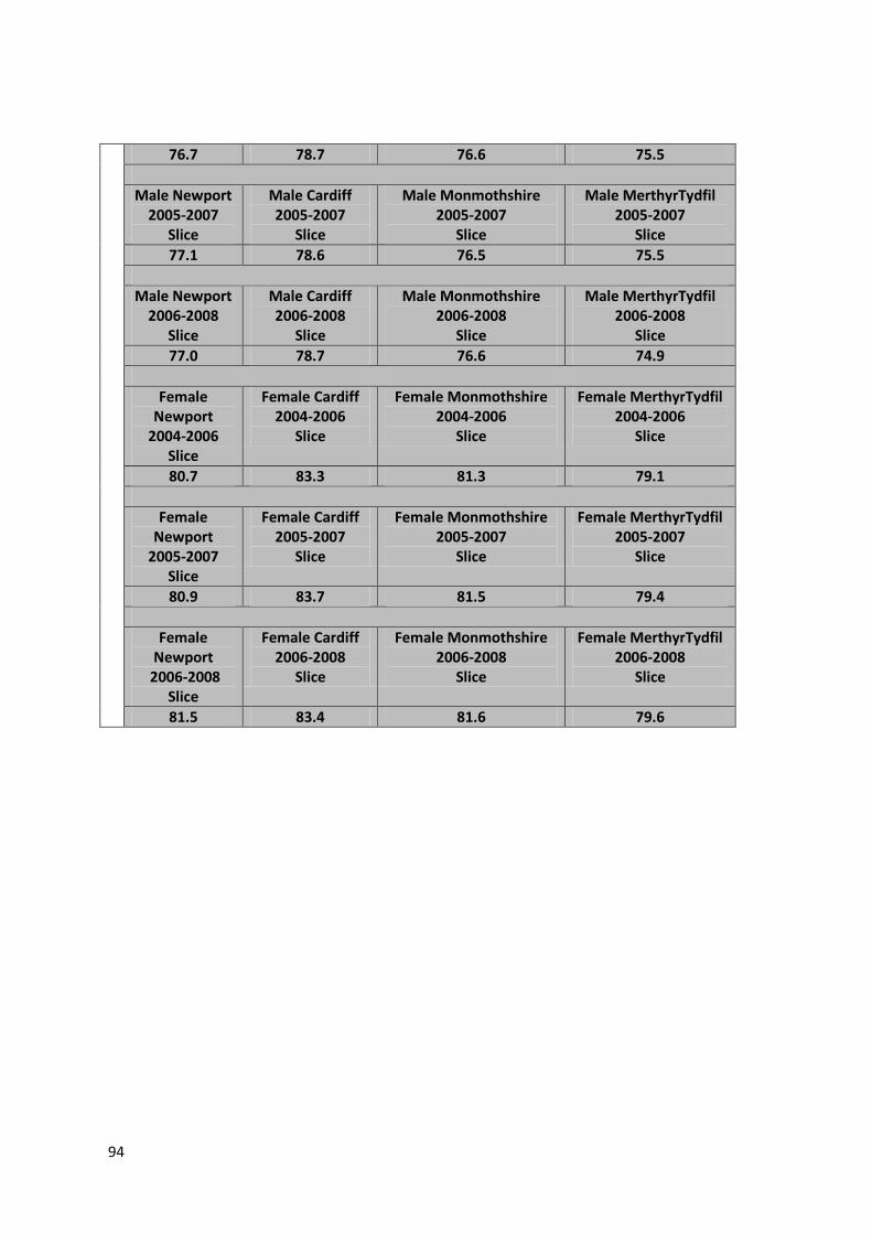
94
76.7 78.7 76.6 75.5
Male Newport 2005-2007
Slice
Male Cardiff 2005-2007
Slice
Male Monmothshire 2005-2007
Slice
Male MerthyrTydfil 2005-2007
Slice
77.1 78.6 76.5 75.5
Male Newport 2006-2008
Slice
Male Cardiff 2006-2008
Slice
Male Monmothshire 2006-2008
Slice
Male MerthyrTydfil 2006-2008
Slice
77.0 78.7 76.6 74.9
Female Newport
2004-2006 Slice
Female Cardiff 2004-2006
Slice
Female Monmothshire 2004-2006
Slice
Female MerthyrTydfil 2004-2006
Slice
80.7 83.3 81.3 79.1
Female Newport
2005-2007 Slice
Female Cardiff 2005-2007
Slice
Female Monmothshire 2005-2007
Slice
Female MerthyrTydfil 2005-2007
Slice
80.9 83.7 81.5 79.4
Female Newport
2006-2008 Slice
Female Cardiff 2006-2008
Slice
Female Monmothshire 2006-2008
Slice
Female MerthyrTydfil 2006-2008
Slice
81.5 83.4 81.6 79.6
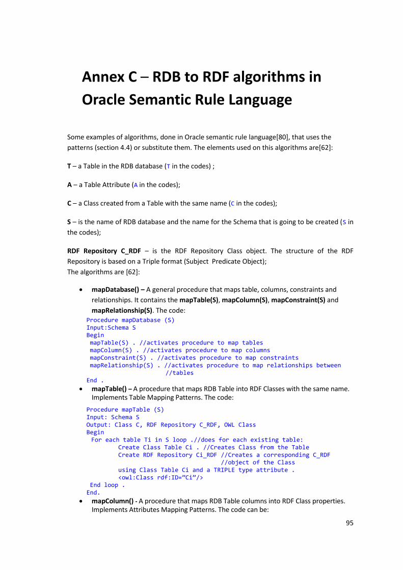
95
Annex C – RDB to RDF algorithms in
Oracle Semantic Rule Language
Some examples of algorithms, done in Oracle semantic rule language[80], that uses the
patterns (section 4.4) or substitute them. The elements used on this algorithms are[62]:
T – a Table in the RDB database (T in the codes) ;
A – a Table Attribute (A in the codes);
C – a Class created from a Table with the same name (C in the codes);
S – is the name of RDB database and the name for the Schema that is going to be created (S in
the codes);
RDF Repository C_RDF – is the RDF Repository Class object. The structure of the RDF
Repository is based on a Triple format (Subject Predicate Object);
The algorithms are [62]:
mapDatabase() – A general procedure that maps table, columns, constraints and
relationships. It contains the mapTable(S), mapColumn(S), mapConstraint(S) and
mapRelationship(S). The code:
Procedure mapDatabase (S) Input:Schema S Begin mapTable(S) . //activates procedure to map tables mapColumn(S) . //activates procedure to map columns mapConstraint(S) . //activates procedure to map constraints mapRelationship(S) . //activates procedure to map relationships between
//tables End .
mapTable() – A procedure that maps RDB Table into RDF Classes with the same name. Implements Table Mapping Patterns. The code:
Procedure mapTable (S) Input: Schema S Output: Class C, RDF Repository C_RDF, OWL Class Begin For each table Ti in S loop .//does for each existing table: Create Class Table Ci . //Creates Class from the Table Create RDF Repository Ci_RDF //Creates a corresponding C_RDF //object of the Class using Class Table Ci and a TRIPLE type attribute . <owl:Class rdf:ID=”Ci”/> End loop . End.
mapColumn() - A procedure that maps RDB Table columns into RDF Class properties. Implements Attributes Mapping Patterns. The code can be:
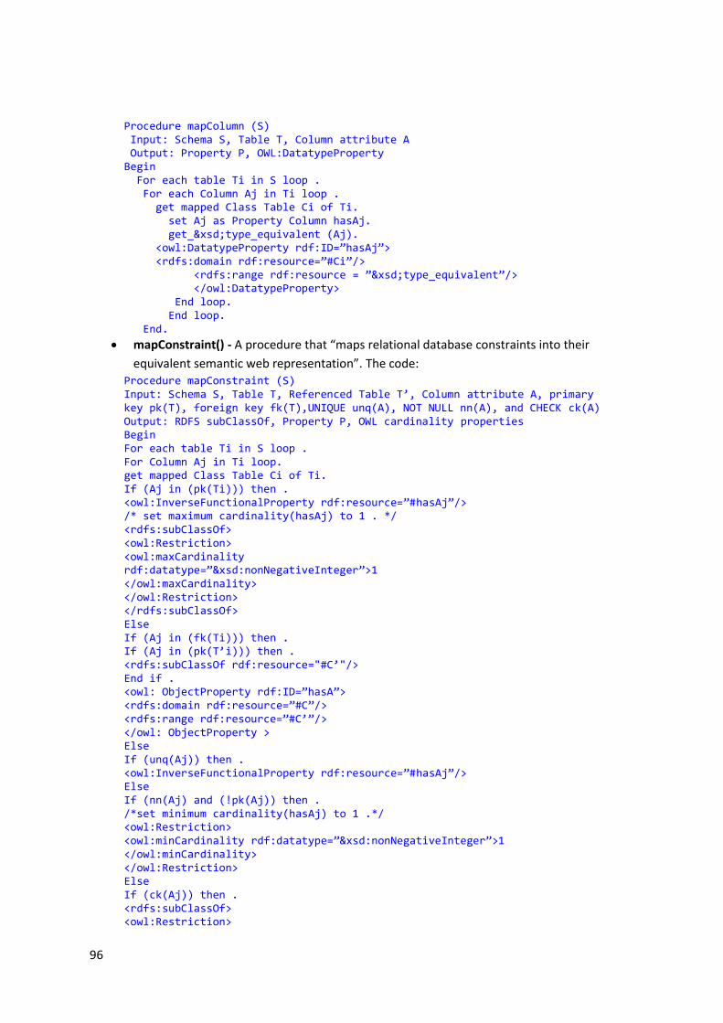
96
Procedure mapColumn (S) Input: Schema S, Table T, Column attribute A Output: Property P, OWL:DatatypeProperty Begin For each table Ti in S loop . For each Column Aj in Ti loop . get mapped Class Table Ci of Ti. set Aj as Property Column hasAj. get_&xsd;type_equivalent (Aj). <owl:DatatypeProperty rdf:ID=”hasAj”> <rdfs:domain rdf:resource=”#Ci”/> <rdfs:range rdf:resource = ”&xsd;type_equivalent”/> </owl:DatatypeProperty> End loop. End loop. End.
mapConstraint() - A procedure that “maps relational database constraints into their
equivalent semantic web representation”. The code: Procedure mapConstraint (S) Input: Schema S, Table T, Referenced Table T’, Column attribute A, primary key pk(T), foreign key fk(T),UNIQUE unq(A), NOT NULL nn(A), and CHECK ck(A) Output: RDFS subClassOf, Property P, OWL cardinality properties Begin For each table Ti in S loop . For Column Aj in Ti loop. get mapped Class Table Ci of Ti. If (Aj in (pk(Ti))) then . <owl:InverseFunctionalProperty rdf:resource=”#hasAj”/> /* set maximum cardinality(hasAj) to 1 . */ <rdfs:subClassOf> <owl:Restriction> <owl:maxCardinality rdf:datatype=”&xsd:nonNegativeInteger”>1 </owl:maxCardinality> </owl:Restriction> </rdfs:subClassOf> Else If (Aj in (fk(Ti))) then . If (Aj in (pk(T’i))) then . <rdfs:subClassOf rdf:resource="#C’"/> End if . <owl: ObjectProperty rdf:ID=”hasA”> <rdfs:domain rdf:resource=”#C”/> <rdfs:range rdf:resource=”#C’”/> </owl: ObjectProperty > Else If (unq(Aj)) then . <owl:InverseFunctionalProperty rdf:resource=”#hasAj”/> Else If (nn(Aj) and (!pk(Aj)) then . /*set minimum cardinality(hasAj) to 1 .*/ <owl:Restriction> <owl:minCardinality rdf:datatype=”&xsd:nonNegativeInteger”>1 </owl:minCardinality> </owl:Restriction> Else If (ck(Aj)) then . <rdfs:subClassOf> <owl:Restriction>
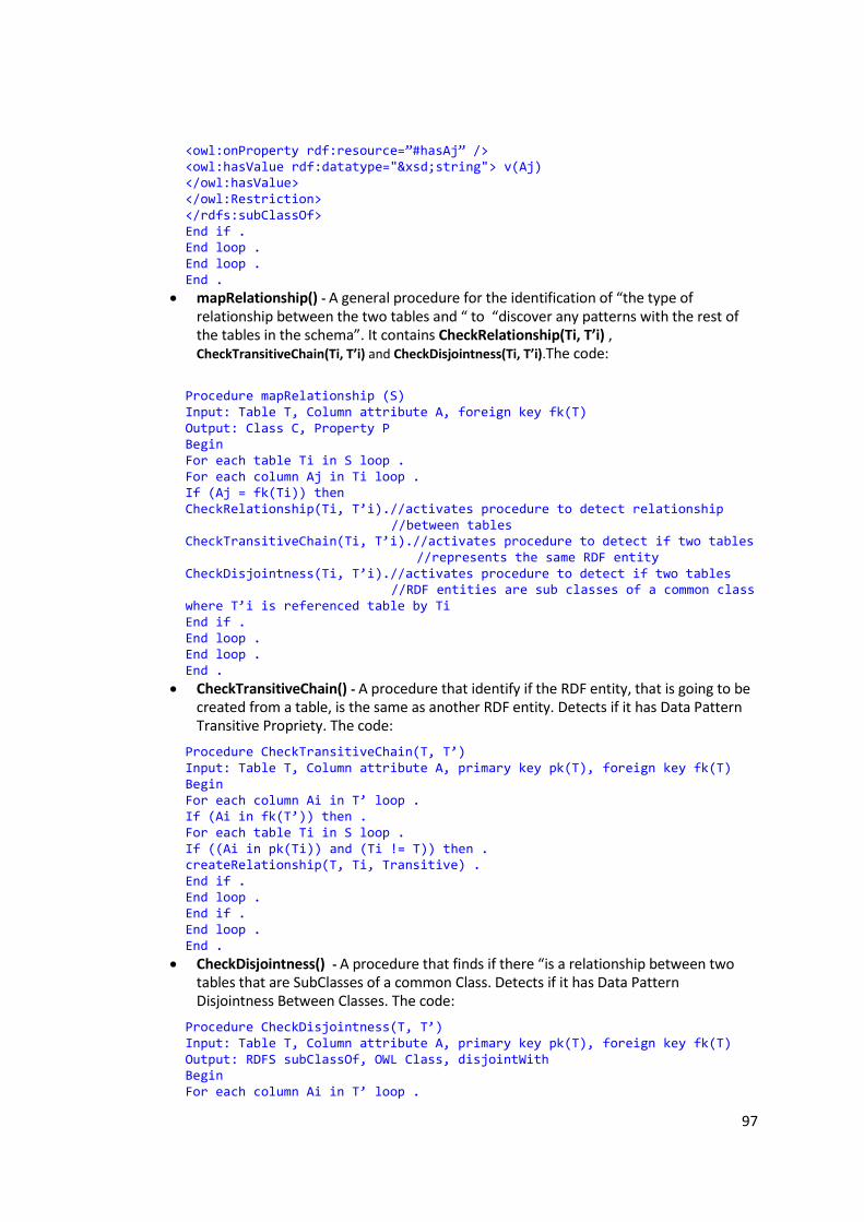
97
<owl:onProperty rdf:resource=”#hasAj” /> <owl:hasValue rdf:datatype="&xsd;string"> v(Aj) </owl:hasValue> </owl:Restriction> </rdfs:subClassOf> End if . End loop . End loop . End .
mapRelationship() - A general procedure for the identification of “the type of relationship between the two tables and “ to “discover any patterns with the rest of the tables in the schema”. It contains CheckRelationship(Ti, T’i) , CheckTransitiveChain(Ti, T’i) and CheckDisjointness(Ti, T’i).The code:
Procedure mapRelationship (S) Input: Table T, Column attribute A, foreign key fk(T) Output: Class C, Property P Begin For each table Ti in S loop . For each column Aj in Ti loop . If (Aj = fk(Ti)) then CheckRelationship(Ti, T’i).//activates procedure to detect relationship
//between tables CheckTransitiveChain(Ti, T’i).//activates procedure to detect if two tables
//represents the same RDF entity CheckDisjointness(Ti, T’i).//activates procedure to detect if two tables
//RDF entities are sub classes of a common class where T’i is referenced table by Ti End if . End loop . End loop . End .
CheckTransitiveChain() - A procedure that identify if the RDF entity, that is going to be created from a table, is the same as another RDF entity. Detects if it has Data Pattern Transitive Propriety. The code:
Procedure CheckTransitiveChain(T, T’) Input: Table T, Column attribute A, primary key pk(T), foreign key fk(T) Begin For each column Ai in T’ loop . If (Ai in fk(T’)) then . For each table Ti in S loop . If ((Ai in pk(Ti)) and (Ti != T)) then . createRelationship(T, Ti, Transitive) . End if . End loop . End if . End loop . End .
CheckDisjointness() - A procedure that finds if there “is a relationship between two tables that are SubClasses of a common Class. Detects if it has Data Pattern Disjointness Between Classes. The code:
Procedure CheckDisjointness(T, T’) Input: Table T, Column attribute A, primary key pk(T), foreign key fk(T) Output: RDFS subClassOf, OWL Class, disjointWith Begin For each column Ai in T’ loop .
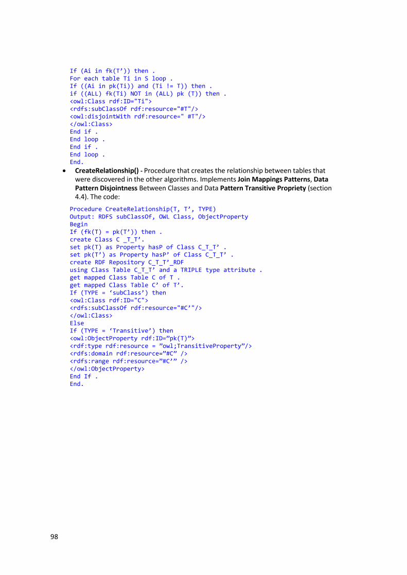
98
If (Ai in fk(T’)) then . For each table Ti in S loop . If ((Ai in pk(Ti)) and (Ti != T)) then . if ((ALL) fk(Ti) NOT in (ALL) pk (T)) then . <owl:Class rdf:ID="Ti"> <rdfs:subClassOf rdf:resource="#T"/> <owl:disjointWith rdf:resource=" #T"/> </owl:Class> End if . End loop . End if . End loop . End.
CreateRelationship() - Procedure that creates the relationship between tables that were discovered in the other algorithms. Implements Join Mappings Patterns, Data Pattern Disjointness Between Classes and Data Pattern Transitive Propriety (section 4.4). The code:
Procedure CreateRelationship(T, T’, TYPE) Output: RDFS subClassOf, OWL Class, ObjectProperty Begin If (fk(T) = pk(T’)) then . create Class C _T_T’. set pk(T) as Property hasP of Class C_T_T’ . set pk(T’) as Property hasP’ of Class C_T_T’ . create RDF Repository C_T_T’_RDF using Class Table C_T_T’ and a TRIPLE type attribute . get mapped Class Table C of T . get mapped Class Table C’ of T’. If (TYPE = ‘subClass’) then <owl:Class rdf:ID="C"> <rdfs:subClassOf rdf:resource="#C’"/> </owl:Class> Else If (TYPE = ‘Transitive’) then <owl:ObjectProperty rdf:ID=”pk(T)”> <rdf:type rdf:resource = ”owl;TransitiveProperty”/> <rdfs:domain rdf:resource=”#C” /> <rdfs:range rdf:resource=”#C’” /> </owl:ObjectProperty> End If . End.


![Dnevni avaz [broj 5607, 11.4.2011]](https://img.pdfslide.net/doc/110x75/53f121f7397c8a60528b4aab/dnevni-avaz-broj-5607-1142011.jpg)