Embed Size (px)
Citation preview
Ocean Modelling 99 (2016) 110–132
Contents lists available at ScienceDirect
Ocean Modelling
journal homepage: www.elsevier.com/locate/ocemod
An assessment of the Arctic Ocean in a suite of interannual CORE-II
simulations. Part I: Sea ice and solid freshwater
Qiang Wang a,∗, Mehmet Ilicak b, Rüdiger Gerdes a, Helge Drange c, Yevgeny Aksenov d,David A. Bailey e, Mats Bentsen b, Arne Biastoch f, Alexandra Bozec g, Claus Böning f,Christophe Cassou h, Eric Chassignet g, Andrew C. Coward d, Beth Curry i,Gokhan Danabasoglu e, Sergey Danilov a, Elodie Fernandez h, Pier Giuseppe Fogli j,Yosuke Fujii k, Stephen M. Griffies l, Doroteaciro Iovino j, Alexandra Jahn e,m, Thomas Jung a,n,William G. Large e, Craig Lee i, Camille Lique o,p, Jianhua Lu g, Simona Masina j,t,A.J. George Nurser d, Benjamin Rabe a, Christina Roth f, David Salas y Mélia q,Bonita L. Samuels l, Paul Spence r,s, Hiroyuki Tsujino k, Sophie Valcke h, Aurore Voldoire q,Xuezhu Wang a, Steve G. Yeager e
a Alfred Wegener Institute, Helmholtz Centre for Polar and Marine Research (AWI), Bremerhaven, Germanyb Uni Research Ltd., Bergen, Norwayc University of Bergen, Bergen, Norwayd National Oceanography Centre (NOC), Southampton SO14 3ZH, UKe National Center for Atmospheric Research (NCAR), Boulder, CO, USAf GEOMAR Helmholtz Centre for Ocean Research, Kiel, Germanyg Center for Ocean-Atmospheric Prediction Studies (COAPS), Florida State University, Tallahassee, FL, USAh Centre Européen de Recherche et de Formation Avancée en Calcul Scientifique (CERFACS), Toulouse, Francei Applied Physics Laboratory, University of Washington, Seattle, Washington, USAj Centro Euro-Mediterraneo sui Cambiamenti Climatici (CMCC), Bologna, Italyk Meteorological Research Institute (MRI), Japan Meteorological Agency, Tsukuba, Japanl NOAA Geophysical Fluid Dynamics Laboratory (GFDL), Princeton, NJ, USAm Department of Atmospheric and Oceanic Sciences and Institute of Arctic and Alpine Research, University of Colorado, Boulder, CO, USAn Institute of Environmental Physics, University of Bremen, Bremen, Germanyo Department of Earth Sciences, University of Oxford, Oxford, UKp Laboratoire de Physique des Océans, Ifremer, centre de Brest, Plouzané, Franceq Centre National de Recherches Météorologiques (CNRM), Toulouse, Francer Climate Change Research Centre, University of New South Wales, Sydney, Australias ARC Centre of Excellence for Climate System Science, University of New South Wales, Sydney, Australiat Istituto Nazionale di Geofisica e Vulcanologia (INGV), Bologna, Italy
a r t i c l e i n f o
Article history:
Received 13 October 2015
Revised 27 November 2015
Accepted 14 December 2015
Available online 4 January 2016
Keywords:
Arctic Ocean
Sea ice
Freshwater
CORE II atmospheric forcing
a b s t r a c t
The Arctic Ocean simulated in fourteen global ocean-sea ice models in the framework of the Coordinated
Ocean-ice Reference Experiments, phase II (CORE II) is analyzed. The focus is on the Arctic sea ice extent,
the solid freshwater (FW) sources and solid freshwater content (FWC). Available observations are used for
model evaluation. The variability of sea ice extent and solid FW budget is more consistently reproduced
than their mean state in the models. The descending trend of September sea ice extent is well simulated
in terms of the model ensemble mean. Models overestimating sea ice thickness tend to underestimate the
descending trend of September sea ice extent. The models underestimate the observed sea ice thinning
trend by a factor of two. When averaged on decadal time scales, the variation of Arctic solid FWC is
contributed by those of both sea ice production and sea ice transport, which are out of phase in time.
The solid FWC decreased in the recent decades, caused mainly by the reduction in sea ice thickness. The
∗ Corresponding author. Tel.: +49 471 48311762.
E-mail address: [email protected] (Q. Wang).
http://dx.doi.org/10.1016/j.ocemod.2015.12.008
1463-5003/© 2015 Elsevier Ltd. All rights reserved.
Q. Wang et al. / Ocean Modelling 99 (2016) 110–132 111
models did not simulate the ac
solid FWC trend after 2000. Th
trend of sea ice thickness and M
1
t
i
g
m
m
n
C
2
B
e
d
t
F
t
t
G
c
t
fl
W
o
t
k
b
b
2
p
s
i
a
M
o
2
i
s
t
M
p
t
I
h
t
a
t
m
t
a
b
m
i
o
s
A
f
u
s
o
r
u
i
t
t
m
o
t
s
w
t
p
t
a
u
t
1
p
f
n
s
c
t
s
e
f
z
n
i
d
p
1
r
A
M
F
a
t
I
i
t
a
1 The analysis done for this paper discovered a bug in the CERFACS NEMO model.
The NEMO grid is folded at the North Pole for an entire grid line going from Canada
to Asia at 78◦W. On this specific grid line, the wind forcing fields need to be rotated
onto the local grid coordinates. This is not correctly done in the CERFACS simula-
tion, leading to spurious signals in ice dynamical fields (e.g., as shown by the sea
ice concentration in Fig. 4). It is found that this bug has a very local imprint and
did not significantly influence the freshwater budget analyzed in this work.
. Introduction
The Arctic Ocean is an important component of the climate sys-
em. It closely interacts with the atmosphere at the surface and
s connected with the large scale ocean circulation through its
ateways. Sea ice, a unique feature of the high latitude oceans,
odifies the planetary albedo and impacts on the air-sea heat, mo-
entum, mass and gas exchange. Arctic sea ice has retreated sig-
ificantly in recent years (Kwok and Rothrock, 2009; Comiso, 2012;
avalieri and Parkinson, 2012; Stroeve et al., 2012a; Laxon et al.,
013), causing amplified warming in the Arctic region (Serreze and
arry, 2011) and far-reaching impact on the Earth System (Bhatt
t al., 2014). The Arctic Ocean is a large freshwater (FW) reservoir
ue to river runoff, net precipitation (P-E) and FW import from
he Pacific (Serreze et al., 2006; Dickson et al., 2007). The excess
W is exported to the subpolar North Atlantic, which can influence
he upper ocean stratification and deep water formation, and thus
he meridional overturning circulation (e.g., Aagaard et al., 1985;
oosse et al., 1997; Hakkinen, 1999; Wadley and Bigg, 2002; Jung-
laus et al., 2005). At depth the intermediate water leaves the Arc-
ic Ocean through Fram Strait, supplying dense waters that over-
ow into the Atlantic proper and then feed the North Atlantic Deep
ater (Rudels and Friedrich, 2000; Karcher et al., 2011). Because
f its essential role in the climate system, understanding the func-
ioning of the Arctic Ocean and predicting its future are among the
ey topics of climate research.
Improved understanding of the Arctic Ocean has been achieved
y using both observations and numerical simulations (see reviews
y Proshutinsky et al., 2011; Haine et al., 2015; Carmack et al.,
015). As model uncertainty can impact on the robustness of both
hysical mechanisms and climate changes inferred from model
imulations, assessment of model performance is necessary. Model
ntercomparison is a useful method to illustrate model consistency
nd spread, thus helping to identify required model improvements.
odel intercomparisons for the Arctic Ocean have been carried
ut based on both coupled climate models (e.g., Holland et al.,
007; Rawlins et al., 2010; Stroeve et al., 2012a) and forced ocean-
ce models (e.g., Holloway et al., 2007; Karcher et al., 2007; John-
on et al., 2007; Jahn et al., 2012a; Johnson et al., 2012). The lat-
er studies are based on models participating in the Arctic Ocean
odel Intercomparison Project (AOMIP, Proshutinsky et al., 2011).
In this work we analyze and compare the ocean and sea ice
roperties in the Arctic Ocean simulated by models participating in
he Coordinated Ocean-ice Reference Experiments, phase II (CORE-
I) project. Model intercomparison under the CORE-II framework
as a few advantages. First, all ocean-ice models are driven by
he same atmospheric state, the CORE interannual forcing (Large
nd Yeager, 2009), and use the same (NCAR) bulk formulae (see
he CORE-II protocol described by Griffies et al. (2012)). A com-
on atmospheric state helps to isolate model-dependent uncer-
ainty from that induced by different atmospheric states. Second,
ll participating models are global ocean-ice models, which have
een used in different coupled climate models. Many of these cli-
ate models have participated in the Climate Model Intercompar-
son Project (CMIP). Model (in)consistency diagnosed from these
cean-ice models can provide information not only to Arctic re-
earchers, but also to climate model developers for improving their
rctic Ocean components. Third, model intercomparisons for dif-
celeration of sea ice thickness decline, leading to an underestimation of
e common model behavior, including the tendency to underestimate the
arch sea ice extent, remains to be improved.
© 2015 Elsevier Ltd. All rights reserved.
erent topics and regions of the world ocean are done in parallel
nder the CORE-II framework (see other papers in this special is-
ue). The combination of these studies will provide an overall view
n the current status of global ocean-ice models used in climate
esearch. We hope that the joint efforts can provide information
seful to improve overall climate model integrity.
Our focus in the CORE-II Arctic framework is on the Arctic sea
ce extent and concentration, the solid and liquid FW budget, and
he Arctic intermediate water layer. We discuss which characteris-
ics are more consistently simulated in the models and what com-
on issues exist among them. Comparisons are made to available
bservations. We will compare and discuss the simulated proper-
ies, but their impact on the large scale circulation is beyond the
cope of this work. We try to present the model intercomparison
ith a broad view including the three major Arctic topics men-
ioned above. This is in line with the pedagogic aspect of the CORE
roject. In order to maintain the readability we split the large con-
ent into three papers. This paper deals with Arctic sea ice extent
nd solid freshwater. The other two papers focus on the Arctic liq-
id freshwater (Wang et al., 2015) and the hydrography in the Arc-
ic Ocean (Ilicak et al., 2015) respectively.
.1. Participating models
Data from fourteen CORE-II models are analyzed in this pa-
er. Thirteen of them were described in the first CORE-II paper
ocused on the North Atlantic (Danabasoglu et al., 2014)1. One
ew model is the global 0.25◦ MOM. Adding it to the analysis
erves to provide information on how fine horizontal grid spacing
an influence simulation results. The models are listed in Table 1,
ogether with the groups names operating the models and the ba-
ic model configuration information. Seven different sea ice mod-
ls are used in the fourteen ocean-ice models (see Appendix A
or descriptions of the sea ice models). Most of the models use
-level (or z∗) coordinates, except for three models with isopyc-
al or hybrid vertical grids (GOLD, FSU and Bergen). One model
s an unstructured-mesh model (AWI-FESOM), configured with tra-
itional climate model resolution for the purpose of the CORE-II
roject. Among the participating models, ten models have nominal◦ horizontal resolution, three with 0.5◦, and one with 0.25◦. The
esolution in km varies significantly in space and direction in the
rctic Ocean, so we can only give very approximate mean values.
OM0.25 has about 12 km horizontal resolution, Kiel-ORCA05 and
ESOM have about 24 km, and the other models have about 48 km.
One of the participating models, MRI-A, is a global ocean data
ssimilation system. It is the same as MRI-F except that tempera-
ure and salinity observational data are assimilated into the model.
t was run for 70 years starting from model year 231 of the MRI-F
ntegration. The first 10 years are treated as a spin-up phase and
he last 60 years (associated with the period of CORE-II forcing)
re used in this work. Its results are compared to other models to
112 Q. Wang et al. / Ocean Modelling 99 (2016) 110–132
Table 1
Summary of the ocean and sea-ice models in alphabetical order according to the participating group name (first column). The table includes the name of
the combined ocean-sea ice configuration (if any); the ocean model name and its version; the sea-ice model name and its version; vertical coordinate and
number of layers/levels in parentheses; orientation of the horizontal grid with respect to the North Pole/Arctic; the number of horizontal grid cells (longitude,
latitude); and the horizontal resolution (longitude, latitude). In MRI-A and MRI-F, the vertical levels shallower than 32 m follow the surface topography as in
sigma-coordinate models. In AWI-FESOM, the total number of surface nodes is given, because it has an unstructured grid. The suite of participating models
include 13 models analyzed in the CORE-II North Atlantic paper (Danabasoglu et al., 2014), and one 0.25◦ fine horizontal grid spacing model (MOM0.25).
FSU-HYCOM has a new model version for the CORE-II study (Danabasoglu et al., 2016), but it is not included in this work.
Group Configuration Ocean model Sea-ice model Vertical Orientation Horiz. grid Horiz. res.
AWI FESOM 1.4 FESIM 2 z (46) Displaced 126000 Nominal 1°Bergen NorESM-O MICOM CICE 4 σ 2 (51 + 2) Tripolar 360 × 384 Nominal 1°CERFACS ORCA1 NEMO 3.2 LIM 2 z (42) Tripolar 360 × 290 Nominal 1°CMCC ORCA1 NEMO 3.3 CICE 4 z (46) Tripolar 360 × 290 Nominal 1◦
CNRM ORCA1 NEMO 3.2 Gelato 5 z (42) Tripolar 360 × 290 Nominal 1◦
FSU HYCOM 2.2 CSIM 5 hybrid (32) Displaced 320 × 384 Nominal 1◦
GFDL-MOM ESM2M-ocean-ice MOM 4p1 SIS1 z∗ (50) Tripolar 360 × 200 Nominal 1◦
GFDL-UNSW MOM0.25 MOM 5 SIS1 z∗ (50) Tripolar 1440 × 1070 Nominal 0.25◦
GFDL-GOLD ESM2G-ocean-ice GOLD SIS1 σ 2 (59 + 4) Tripolar 360 × 210 Nominal 1◦
Kiel ORCA05 NEMO 3.1.1 LIM 2 z (46) Tripolar 722 × 511 Nominal 0.5◦
MRI-A MRI assimilation MOVE/MRI.COM 3 MK89; CICE z (50) Tripolar 360 × 364 1◦ × 0.5◦
MRI-F MRI free run MRI.COM 3 MK89; CICE z (50) Tripolar 360 × 364 1◦ × 0.5◦
NCAR POP 2 CICE 4 z (60) Displaced 320 × 384 Nominal 1◦
NOC ORCA1 NEMO 3.4 LIM 2 z (75) Tripolar 360 × 290 Nominal 1◦
d
p
t
c
t
2
A
e
p
i
s
c
t
w
c
W
N
b
i
c
l
t
p
A
A
i
m
r
A
m
a
s
a
t
g
u
o
i
2 Note that slightly different reference salinity values have also been used in lit-
erature. See the comments on the choice of reference values and the definition of
FW by Bacon et al. (2015) and Carmack et al. (2015).
provide information on whether the assimilation improves the key
diagnostics of the Arctic Ocean. However, we do not include it for
calculating model ensemble means.
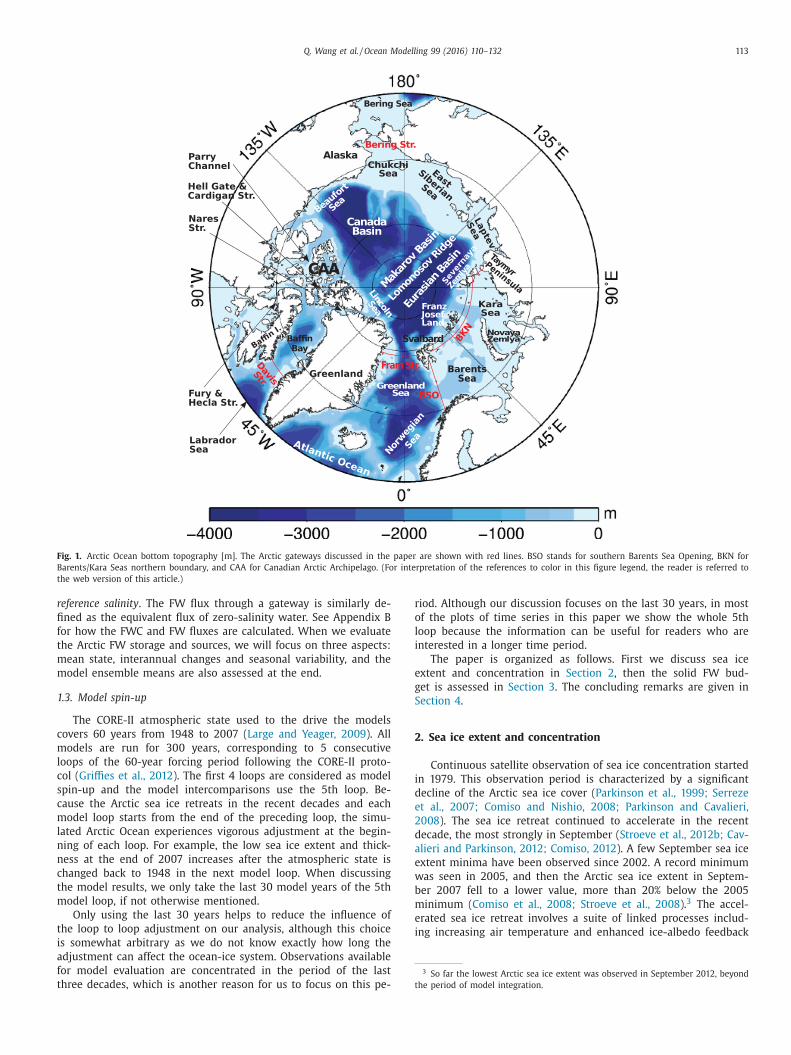
In this paper we define the Arctic Ocean domain with the fol-
lowing four gateways: Bering Strait, Fram Strait, Davis Strait, and
the Barents and Kara Seas northern boundary (BKN) (see Fig. 1).
Bering Strait is the only gateway connecting the Arctic Ocean with
the Pacific. In the Atlantic sector, the Arctic Ocean is connected
with the Nordic Seas via Fram Strait, with the Labrador Sea via
Davis Strait, and with the Barents/Kara Seas then the Nordic Seas
via the BKN. We take Davis Strait rather than the Canadian Arctic
Archipelago (CAA) as one of the Arctic Ocean boundaries for sim-
plicity because the number of CAA passages connecting the Arctic
Ocean and Baffin Bay is different among the models.
Table 1 shows the basic model configurations, therein we list
the models in the alphabetical order with respect to the names of
the contributing groups. In all figures and other tables in this pa-
per, we will group the models according to types of vertical coordi-
nates and model origins, when possible. The five models based on
NEMO are put closer, the same for the two MOM models with dif-
ferent horizontal resolution, the three isopycnal (and hybrid) mod-
els, and the free-run and assimilated MRI models.
1.2. Basic concepts
Sea ice extent. The decline of Arctic sea ice, with possible impact
on different components of the Earth System (Bhatt et al., 2014),
has emerged as a leading signal of global warming. The mean state
and decline of sea ice need to be quantified, often by using the so-
called sea ice extent, which is defined as the sum of ice covered
areas with sea ice concentrations of at least 15%. The sea ice concen-
tration is the fractional area of the ocean covered by sea ice.
Sea ice area, the summed product of the ice concentration and
area of each data element within the ice extent, is another widely
used quantity for describing sea ice cover. In this work we only
assess the simulated sea ice extent, and note that the descend-
ing trends of Arctic sea ice extent and area are different, especially
when compared for particular regions and seasons (Cavalieri and
Parkinson, 2012; Comiso, 2012).
For evaluating the sea ice extent, we compare both the sim-
ulated mean state and trend with satellite observations (Fetterer
et al., 2002). The comparison is made for September and March
when the Northern Hemisphere (NH) sea ice extent has minimum
and maximum, respectively (note that the maximal and minimal
escending trends are in September and May, respectively, for the
eriod of 1979–2010 (Cavalieri and Parkinson, 2012)). In addition
o the total NH sea ice extent, we also evaluate the models for one
hosen region, the Barents Sea, where most significant sea ice re-
reat is predicted in simulations of future climate (Koenigk et al.,
013).
rctic freshwater. The Arctic Ocean is a big FW reservoir (Serreze
t al., 2006; Dickson et al., 2007). It receives FW as river runoff,
recipitation and inflow from Bering Sea. The amount of FW stored
n the Arctic Ocean is an important index that can be used to de-
cribe the climate status of the Arctic Ocean. The excess FW re-
eived by the Arctic Ocean is finally released to the North Atlantic
hrough Fram and Davis Straits. Due to the proximity to the deep
ater formation sites and potential impact on large scale ocean cir-
ulation (Dickson et al., 1988; Goosse et al., 1997; Hakkinen, 2002;
adley and Bigg, 2002), the FW flux from the Arctic Ocean to the
orth Atlantic is one of the key variables describing the linkage
etween the Arctic and subpolar regions.
FW in the Arctic Ocean exists in the solid form mainly as sea
ce and in the liquid form mainly located in the upper ocean. We
all sea ice and particular ocean waters FW because their salinity is
ower than a reference value, which is chosen according to the con-
ext of discussed topics. For example, if one wants to study the im-
act of Arctic FW export on the deep water formation in the North
tlantic, she/he will take the mean salinity of the subpolar North
tlantic as the reference salinity; if one analyzes the FW budget
n the Arctic Ocean, she/he might choose a value representing the
ean state of the Arctic Ocean. In this paper we focus on the Arctic
egion, so we take 34.8, a value close to the mean salinity in the
rctic basins as the reference salinity following Aagaard and Car-
ack (1989) and Serreze et al. (2006). Using this common value
llows us to compare the model results directly with the synthe-
ized Arctic FW budget (Serreze et al., 2006; Haine et al., 2015)
nd analyses in many observational and model studies2.
Understanding the Arctic FW budget involves quantifying both
he Arctic FW storage and sources, including fluxes through the
ateways. The FW storage in the Arctic Ocean can be quantified
sing the so-called freshwater content (FWC), which is the amount
f zero-salinity water required to be taken out from the ocean (or sea
ce) so that the ocean (or sea ice) salinity is changed to the chosen
Q. Wang et al. / Ocean Modelling 99 (2016) 110–132 113
Fig. 1. Arctic Ocean bottom topography [m]. The Arctic gateways discussed in the paper are shown with red lines. BSO stands for southern Barents Sea Opening, BKN for
Barents/Kara Seas northern boundary, and CAA for Canadian Arctic Archipelago. (For interpretation of the references to color in this figure legend, the reader is referred to
the web version of this article.)
r
fi
f
t
m
m
1
c
m
l
c
s
c
m
l
n
n
c
t
m
t
i
a
f
t
r
o
l
i
e
g
S
2
i
d
e
2
d
a
e
w
b
m
e
i
3 So far the lowest Arctic sea ice extent was observed in September 2012, beyond
the period of model integration.
eference salinity. The FW flux through a gateway is similarly de-
ned as the equivalent flux of zero-salinity water. See Appendix B
or how the FWC and FW fluxes are calculated. When we evaluate
he Arctic FW storage and sources, we will focus on three aspects:
ean state, interannual changes and seasonal variability, and the
odel ensemble means are also assessed at the end.
.3. Model spin-up
The CORE-II atmospheric state used to the drive the models
overs 60 years from 1948 to 2007 (Large and Yeager, 2009). All
odels are run for 300 years, corresponding to 5 consecutive
oops of the 60-year forcing period following the CORE-II proto-
ol (Griffies et al., 2012). The first 4 loops are considered as model
pin-up and the model intercomparisons use the 5th loop. Be-
ause the Arctic sea ice retreats in the recent decades and each
odel loop starts from the end of the preceding loop, the simu-
ated Arctic Ocean experiences vigorous adjustment at the begin-
ing of each loop. For example, the low sea ice extent and thick-
ess at the end of 2007 increases after the atmospheric state is
hanged back to 1948 in the next model loop. When discussing
he model results, we only take the last 30 model years of the 5th
odel loop, if not otherwise mentioned.
Only using the last 30 years helps to reduce the influence of
he loop to loop adjustment on our analysis, although this choice
s somewhat arbitrary as we do not know exactly how long the
djustment can affect the ocean-ice system. Observations available
or model evaluation are concentrated in the period of the last
hree decades, which is another reason for us to focus on this pe-
iod. Although our discussion focuses on the last 30 years, in most
f the plots of time series in this paper we show the whole 5th
oop because the information can be useful for readers who are
nterested in a longer time period.
The paper is organized as follows. First we discuss sea ice
xtent and concentration in Section 2, then the solid FW bud-
et is assessed in Section 3. The concluding remarks are given in
ection 4.
. Sea ice extent and concentration
Continuous satellite observation of sea ice concentration started
n 1979. This observation period is characterized by a significant
ecline of the Arctic sea ice cover (Parkinson et al., 1999; Serreze
t al., 2007; Comiso and Nishio, 2008; Parkinson and Cavalieri,
008). The sea ice retreat continued to accelerate in the recent
ecade, the most strongly in September (Stroeve et al., 2012b; Cav-
lieri and Parkinson, 2012; Comiso, 2012). A few September sea ice
xtent minima have been observed since 2002. A record minimum
as seen in 2005, and then the Arctic sea ice extent in Septem-
er 2007 fell to a lower value, more than 20% below the 2005
inimum (Comiso et al., 2008; Stroeve et al., 2008).3 The accel-
rated sea ice retreat involves a suite of linked processes includ-
ng increasing air temperature and enhanced ice-albedo feedback
114 Q. Wang et al. / Ocean Modelling 99 (2016) 110–132
Ta
ble
2
No
rth
ern
He
mis
ph
ere
(NH
)se
aic
ee
xte
nt:
me
an
,st
an
da
rdd
ev
iati
on
(ST
D),
corr
ela
tio
nw
ith
ob
serv
ati
on
,li
ne
ar
tre
nd
,a
nd
the
20
07
va
lue
.T
he
last
two
colu
mn
ssh
ow
the
mo
de
le
nse
mb
lem
ea
na
nd
spre
ad
.1
Ob
serv
ati
on
NC
AR
AW
IM
OM
MO
M0
.25
CE
RFA
CS
CN
RM
Kie
lN
OC
CM
CC
MR
I-F
MR
I-A
GO
LDF
SU
Be
rge
nM
ea
nS
pre
ad
Se
pte
mb
er
Me
an
6.9
53
.99
8.1
86
.30
5.9
68
.12
6.4
67
.85
7.7
62
.14
7.6
56
.84
6.5
24
.00
5.2
76
.17
1.8
7
ST
D0
.58
1.4
40
.61
0.8
90
.66
0.4
20
.86
0.4
30
.49
1.0
40
.57
0.6
10
.98
1.5
41
.47
0.8
80
.40
Co
rre
lati
on
0.7
10
.76
0.6
30
.73
0.6
70
.67
0.7
40
.64
0.6
80
.79
0.8
00
.62
0.7
20
.60
0.6
90
.06
Tre
nd
79
–0
3−5
.3−1
1.0
−2.7
−6.4
−4.4
−2.5
−5.9
−2.1
−2.6
−5.2
−3.5
−4.2
−7.5
−10
.9−1
2.8
−6.0
3.6
Tre
nd
79
–0
7−7
.2−1
1.3
−4.9
−8.9
−5.5
−4.3
−8.5
−3.9
−4.5
−6.0
−5.4
−4.9
−9.0
−10
.4−1
3.6
−7.2
3.0
20
07
ice
ex
ten
t4
.30
1.2
16
.09
3.1
24
.31
6.3
43
.23
6.3
15
.80
0.6
45
.69
5.2
63
.89
1.9
31
.98
3.8
92
.04
Ma
rch
Me
an
15
.72
15
.20
15
.98
16
.06
14
.78
15
.66
15
.38
14
.78
15
.87
14
.57
15
.33
14
.43
16
.40
16
.60
15
.06
15
.51
0.6
4
ST
D0
.34
0.2
20
.25
0.2
20
.24
0.2
10
.15
0.2
40
.28
0.2
00
.29
0.3
80
.24
0.2
90
.21
0.2
40
.04
Co
rre
lati
on
0.6
50
.66
0.6
00
.76
0.5
90
.76
0.6
50
.46
0.8
00
.45
0.3
70
.68
0.2
10
.67
0.6
10
.16
Tre
nd
79
–0
3−3
.4−1
.4−1
.3−1
.1−1
.6−1
.3−0
.7−0
.9−1
.8−1
.2−2
.1−3
.3−0
.9−1
.3−1
.7−1
.30
.4
Tre
nd
79
–0
7−4
.7−2
.7−3
.1−2
.5−2
.8−2
.7−1
.7−2
.3−3
.5−2
.7−3
.5−4
.8−2
.2−3
.1−2
.6−2
.90
.7
20
07
ice
ex
ten
t1
4.6
51
4.5
01
5.1
91
5.3
21
4.0
41
4.8
51
4.9
01
3.9
71
4.7
41
3.7
71
4.5
21
3.4
51
5.7
71
5.6
31
4.4
21
4.7
40
.62
1S
ea
ice
ex
ten
tis
in1
06
km
2,
an
dth
etr
en
dis
in1
04
km
2/y
ea
r.T
he
sta
tist
ics
are
calc
ula
ted
for
Se
pte
mb
er
an
dM
arc
hm
on
thly
da
tase
pa
rate
ly.
We
use
the
pe
rio
d1
97
9–
20
03
toca
lcu
late
the
me
an
va
lue
so
fse
aic
ee
xte
nt,
its
sta
nd
ard
de
via
tio
n(S
TD
),co
rre
lati
on
wit
hth
eo
bse
rva
tio
n,
an
dth
eli
ne
ar
tre
nd
.T
he
lin
ea
rtr
en
dfo
rth
ep
eri
od
19
79
–2
00
7is
als
oca
lcu
late
d.
Th
eco
rre
lati
on
coe
ffici
en
tsa
reca
lcu
late
da
fte
rth
eli
ne
ar
tre
nd
isre
mo
ve
d.
Th
eo
bse
rva
tio
nis
ba
sed
on
the
sea
ice
ind
ex
pro
vid
ed
by
Fett
ere
re
ta
l.(2
00
2).
No
teth
at
the
ass
imil
ati
on
mo
de
lM
RI-
Ais
no
tu
sed
inth
eca
lcu
lati
on
of
the
mo
de
le
nse
mb
lem
ea
na
nd
spre
ad
,th
esa
me
as
ino
the
rta
ble
s
an
dfi
gu
res.
(Stroeve et al., 2012b), and contributes to amplified Arctic warm-
ing (Serreze and Barry, 2011).
Due to its crucial roles in the climate system, the status of sea
ice is among the key model variables that need to be evaluated. In
this section we assess the Northern Hemisphere (NH) sea ice ex-
tent and concentration simulated in the CORE-II models by com-
paring to the satellite observations, which are regularly updated
(Fetterer et al., 2002). The mean state and trend of NH sea ice ex-
tent is discussed in Sections 2.1 and 2.2, respectively. The Arctic
sea ice declines regionally at different rates (Cavalieri and Parkin-
son, 2012), so it is also interesting to assess the simulated sea ice
on a regional basis. In this paper we do not attempt to compare
all the Arctic regions, and only focus on one particular shelf sea,
the Barents Sea, where most significant sea ice retreat is predicted
in simulations of future climate (Koenigk et al., 2013). This is pre-
sented in Section 2.3. A summary on the model ensemble mean is
given in Section 2.4.
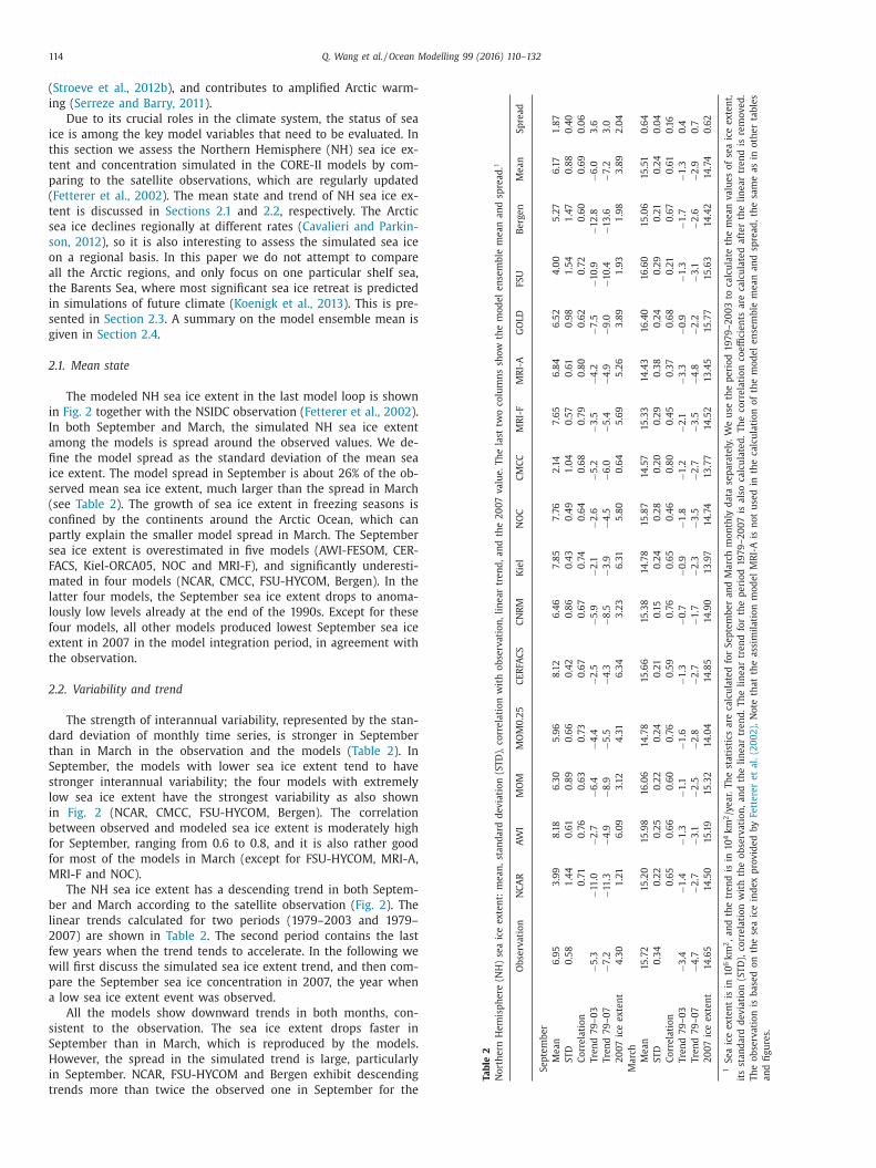
2.1. Mean state
The modeled NH sea ice extent in the last model loop is shown
in Fig. 2 together with the NSIDC observation (Fetterer et al., 2002).
In both September and March, the simulated NH sea ice extent
among the models is spread around the observed values. We de-
fine the model spread as the standard deviation of the mean sea
ice extent. The model spread in September is about 26% of the ob-
served mean sea ice extent, much larger than the spread in March
(see Table 2). The growth of sea ice extent in freezing seasons is
confined by the continents around the Arctic Ocean, which can
partly explain the smaller model spread in March. The September
sea ice extent is overestimated in five models (AWI-FESOM, CER-
FACS, Kiel-ORCA05, NOC and MRI-F), and significantly underesti-
mated in four models (NCAR, CMCC, FSU-HYCOM, Bergen). In the
latter four models, the September sea ice extent drops to anoma-
lously low levels already at the end of the 1990s. Except for these
four models, all other models produced lowest September sea ice
extent in 2007 in the model integration period, in agreement with
the observation.
2.2. Variability and trend
The strength of interannual variability, represented by the stan-
dard deviation of monthly time series, is stronger in September
than in March in the observation and the models (Table 2). In
September, the models with lower sea ice extent tend to have
stronger interannual variability; the four models with extremely
low sea ice extent have the strongest variability as also shown
in Fig. 2 (NCAR, CMCC, FSU-HYCOM, Bergen). The correlation
between observed and modeled sea ice extent is moderately high
for September, ranging from 0.6 to 0.8, and it is also rather good
for most of the models in March (except for FSU-HYCOM, MRI-A,
MRI-F and NOC).
The NH sea ice extent has a descending trend in both Septem-
ber and March according to the satellite observation (Fig. 2). The
linear trends calculated for two periods (1979–2003 and 1979–
2007) are shown in Table 2. The second period contains the last
few years when the trend tends to accelerate. In the following we
will first discuss the simulated sea ice extent trend, and then com-
pare the September sea ice concentration in 2007, the year when
a low sea ice extent event was observed.
All the models show downward trends in both months, con-
sistent to the observation. The sea ice extent drops faster in
September than in March, which is reproduced by the models.
However, the spread in the simulated trend is large, particularly
in September. NCAR, FSU-HYCOM and Bergen exhibit descending
trends more than twice the observed one in September for the
Q. Wang et al. / Ocean Modelling 99 (2016) 110–132 115
Year
1950 1960 1970 1980 1990 2000
Ice E
xte
nt
[10
6km
2]
0
2
4
6
8
10September Ice Extent
NCARAWI-FESOMGFDL-MOMMOM0.25Ensemble meanNSIDC
Year
1950 1960 1970 1980 1990 2000
Ice E
xte
nt
[10
6km
2]
12
14
16
18March Ice Extent
NCARAWI-FESOMGFDL-MOMMOM0.25Ensemble meanNSIDC
Year
1950 1960 1970 1980 1990 2000
Ice E
xte
nt
[10
6km
2]
0
2
4
6
8
10CERFACSCNRMKiel-ORCA05NOCCMCCEnsemble meanNSIDC
Year
1950 1960 1970 1980 1990 2000
Ice E
xte
nt
[10
6km
2]
12
14
16
18CERFACSCNRMKiel-ORCA05NOCCMCCEnsemble meanNSIDC
Year
1950 1960 1970 1980 1990 2000
Ice E
xte
nt
[10
6km
2]
0
2
4
6
8
10MRI-FMRI-AGFDL-GOLDFSU-HYCOMBergenEnsemble meanNSIDC
Year
1950 1960 1970 1980 1990 2000
Ice E
xte
nt
[10
6km
2]
12
14
16
18MRI-FMRI-AGFDL-GOLDFSU-HYCOMBergenEnsemble meanNSIDC
Fig. 2. Northern Hemisphere (left) September and (right) March sea ice extent [106 km2] in the last model loop. Note that the assimilation model MRI-A is not used in the
calculation of the model ensemble mean. The observation from NSIDC (Fetterer et al., 2002) is shown with gray lines for the period of 1979–2007.
p
e
a
t
t
t
e
t
F
t
fl
C
f
t
b
i
w
F
c
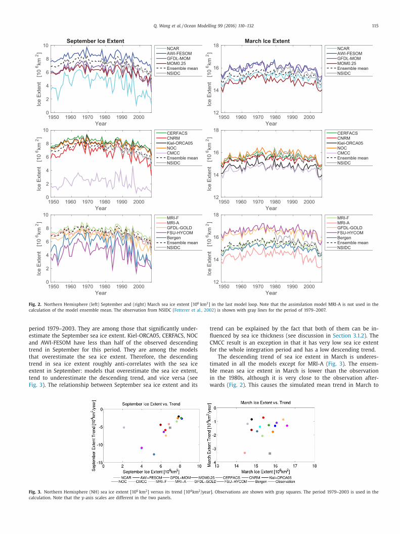
eriod 1979–2003. They are among those that significantly under-
stimate the September sea ice extent. Kiel-ORCA05, CERFACS, NOC
nd AWI-FESOM have less than half of the observed descending
rend in September for this period. They are among the models
hat overestimate the sea ice extent. Therefore, the descending
rend in sea ice extent roughly anti-correlates with the sea ice
xtent in September: models that overestimate the sea ice extent,
end to underestimate the descending trend, and vice versa (see
ig. 3). The relationship between September sea ice extent and its
ig. 3. Northern Hemisphere (NH) sea ice extent [106 km2] versus its trend [104km2/year
alculation. Note that the y-axis scales are different in the two panels.
rend can be explained by the fact that both of them can be in-
uenced by sea ice thickness (see discussion in Section 3.1.2). The
MCC result is an exception in that it has very low sea ice extent
or the whole integration period and has a low descending trend.
The descending trend of sea ice extent in March is underes-
imated in all the models except for MRI-A (Fig. 3). The ensem-
le mean sea ice extent in March is lower than the observation
n the 1980s, although it is very close to the observation after-
ards (Fig. 2). This causes the simulated mean trend in March to
]. Observations are shown with gray squares. The period 1979–2003 is used in the
116 Q. Wang et al. / Ocean Modelling 99 (2016) 110–132
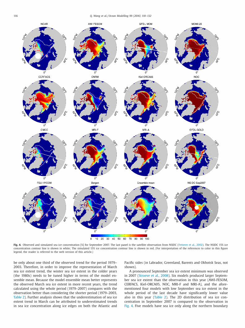
Fig. 4. Observed and simulated sea ice concentration [%] for September 2007. The last panel is the satellite observation from NSIDC (Fetterer et al., 2002). The NSIDC 15% ice
concentration contour line is shown in white; The simulated 15% ice concentration contour line is shown in red. (For interpretation of the references to color in this figure
legend, the reader is referred to the web version of this article.)
P
s
i
b
C
m
w
a
c
F
be only about one third of the observed trend for the period 1979–
2003. Therefore, in order to improve the representation of March
sea ice extent trend, the winter sea ice extent in the colder years
(the 1980s) needs to be tuned higher in terms of the model en-
semble mean. Because the model ensemble mean better represents
the observed March sea ice extent in more recent years, the trend
calculated using the whole period (1979–2007) compares with the
observation better than considering the shorter period (1979–2003,
Table 2). Further analysis shows that the underestimation of sea ice
extent trend in March can be attributed to underestimated trends
in sea ice concentration along ice edges on both the Atlantic and
acific sides (in Labrador, Greenland, Barents and Okhotsk Seas, not
hown).
A pronounced September sea ice extent minimum was observed
n 2007 (Stroeve et al., 2008). Six models produced larger Septem-
er sea ice extent than the observation in this year (AWI-FESOM,
ERFACS, Kiel-ORCA05, NOC, MRI-F and MRI-A), and the afore-
entioned four models with low September sea ice extent in the
hole period of the last decade have significantly lower value
lso in this year (Table 2). The 2D distribution of sea ice con-
entration in September 2007 is compared to the observation in
ig. 4. Five models have sea ice only along the northern boundary
Q. Wang et al. / Ocean Modelling 99 (2016) 110–132 117
Month
2 4 6 8 10 12
Se
a Ice
Exte
nt
[10
6km
2]
0
5
10
15
20Sea Ice Extent
Month
2 4 6 8 10 12
Se
a I
ce
Vo
lum
e[1
04km
3]
0
0.5
1
1.5
2
2.5
3
3.5
4Sea Ice Volume
Fig. 5. Seasonal cycle of Northern Hemisphere (left) sea ice extent [106 km2] and (right) sea ice volume [104 km3] averaged over the years 1979–2007. The model ensemble
means are shown with dashed lines. The gray line in the left panel shows the observed sea ice extent (Fetterer et al., 2002).
o
t
e
S
w
t
i
a
t
s
i
l
2
f
t
i
F
e
s
t
w
2
a
e
B
t
c
i
d
e
i
m
h
m
t
b
r
v
m
i
t
0
t
s
v
b
(
r
i
b
w
t
t
p
e
S
r
t
t
2
s
O
f the CAA, missing the observed sea ice in the central Arctic and
he ice tongue towards the Laptev Sea. In the other nine mod-
ls, the observed sea ice retreat toward the North Pole from the
iberian side is reproduced, but most of these models show a
eaker decline. GFDL-MOM and GFDL-GOLD have ice edges close
o the observation in the western Arctic, but they have too low
ce concentration near the North Pole. On the contrary, MOM0.25
nd NOC have too high sea ice concentration. All the models tend
o have more summer sea ice in the southern CAA than the ob-
ervation4. It was found that the downward shortwave radiation
n the CORE normal year forcing has a negative bias, which can
ead to overestimation of summer sea ice in the CAA (Wang et al.,
012). It is not clear if a similar bias exits in the CORE interannual
orcing.
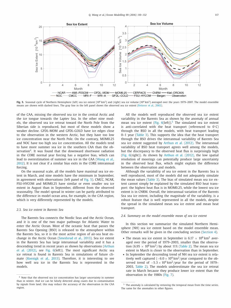
On the seasonal scale, all the models have maximal sea ice ex-
ent in March, and nine models have the minimum in September,
n agreement with observations (left panel of Fig. 5). CMCC, NCAR,
SU-HYCOM and MOM0.25 have similar or even smaller sea ice
xtent in August than in September, different from the observed
easonality. The model spread in winter can be partly attributed to
he difference in model ocean area, for example, in the CAA region,
hich is very differently represented by the models.
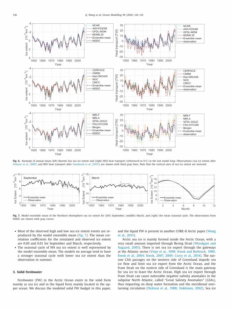
.3. Sea ice extent in Barents Sea
The Barents Sea connects the Nordic Seas and the Arctic Ocean,
nd it is one of the two major pathways for Atlantic Water to
nter the Arctic Ocean. Most of the oceanic heat that passes the
arents Sea Opening (BSO) is released to the atmosphere within
he Barents Sea, so it is the most active region of air-sea heat ex-
hange in the Arctic Ocean (Smedsrud et al., 2013). Sea ice extent
n the Barents Sea has large interannual variability and it has a
escending trend in recent years as shown by observations (Arthun
t al. (2012), see Fig. 6(left)). The most significant Arctic sea
ce retreat is found in Barents Sea in simulations of future cli-
ate (Koenigk et al., 2013). Therefore, it is interesting to see
ow well sea ice in the Barents Sea is represented in the
odels.
4 Note that the observed sea ice concentration has larger uncertainty in summer
han in winter. And ice can be falsely detected along coasts due to contamination
y signals from land; this may reduce the accuracy of the observation in the CAA
egion. T
All the models well reproduced the observed sea ice extent
ariability in the Barents Sea as shown by the anomaly of annual
ean sea ice extent (Fig. 6(left)).5 The simulated sea ice extent
s anti-correlated with the heat transport (referenced to 0◦C)
hrough the BSO in all the models, with heat transport leading
–1 year (Table 3). This supports the idea that the heat transport
hrough the BSO drives the interannual variability of Barents Sea
ea ice extent suggested by Arthun et al. (2012). The interannual
ariability of BSO heat transport agrees well among the models,
ut the discrepancy to the observed heat flux is surprisingly high
Fig. 6(right)). As shown by Arthun et al. (2012), the low spatial
esolution of moorings can potentially produce large uncertainty
n the observed heat flux, which might explain the difference
etween the observation and models.
Although the variability of sea ice extent in the Barents Sea is
ell reproduced, most of the models did not adequately simulate
he mean values (Table 3). The bias of simulated mean sea ice ex-
ent cannot simply be explained by the simulated BSO heat trans-
ort: the highest heat flux is in MOM0.25, while the lowest sea ice
xtent is in CNRM. Overall, the interannual variation of the Barents
ea sea ice extent, including the magnitude of the variability, is a
obust feature that is well represented in all the models, despite
he spread in the simulated mean sea ice extent and mean heat
ransport.
.4. Summary on the model ensemble mean of sea ice extent
In this section we summarize the simulated Northern Hemi-
phere (NH) sea ice extent based on the model ensemble mean.
ther remarks will be given in the concluding section (Section 4).
• The mean sea ice extent in September is 6.17 × 10⁶ km2 aver-
aged over the period of 1979–2003, smaller than the observa-
tion (6.95 × 10⁶ km2) by about 11% (Table 2). The mean sea ice
extent in March is closer to the observation than in September.• In September the descending trend of NH sea ice extent is rela-
tively well captured (−6.0 × 10⁴ km2/year compared to the ob-
served trend of −5.3 × 10⁴ km2/year for the period of 1979–
2003, Table 2). The models underestimate the sea ice retreat
rate in March because they produce lower ice extent than the
observation in the 1980s (Fig. 7).
5 The anomaly is calculated by removing the temporal mean from the time series.
he same for the anomalies in other figures.
118 Q. Wang et al. / Ocean Modelling 99 (2016) 110–132
Year
1950 1960 1970 1980 1990 2000
Ice
exte
nt
[10
5km
2]
4
2
0
-2
-4NCAR
AWI-FESOM
GFDL-MOM
MOM0.25
Ensemble mean
NSIDC
Year
1950 1960 1970 1980 1990 2000
He
at tr
an
sp
ort
[T
W]
-30
-20
-10
0
10
20
30 NCAR
AWI-FESOM
GFDL-MOM
MOM0.25
Ensemble mean
observation
Year
1950 1960 1970 1980 1990 2000
Ice
exte
nt
[10
5km
2]
4
2
0
-2
-4CERFACS
CNRM
Kiel-ORCA05
NOC
CMCC
Ensemble mean
NSIDC
Year
1950 1960 1970 1980 1990 2000
He
at tr
an
sp
ort
[T
W]
-30
-20
-10
0
10
20
30 CERFACS
CNRM
Kiel-ORCA05
NOC
CMCC
Ensemble mean
observation
Year
1950 1960 1970 1980 1990 2000
Ice
exte
nt
[10
5km
2]
4
2
0
-2
-4MRI-F
MRI-A
GFDL-GOLD
FSU-HYCOM
Bergen
Ensemble mean
NSIDC
Year
1950 1960 1970 1980 1990 2000
He
at tr
an
sp
ort
[T
W]
-30
-20
-10
0
10
20
30 MRI-F
MRI-A
GFDL-GOLD
FSU-HYCOM
Bergen
Ensemble mean
observation
Fig. 6. Anomaly of annual mean (left) Barents Sea sea ice extent and (right) BSO heat transport (referenced to 0◦C) in the last model loop. Observations (sea ice extent after
Fetterer et al. (2002) and BSO heat transport after Smedsrud et al. (2013)) are shown with thick gray lines. Note that the vertical axes of sea ice extent are inverted.
Year1950 1960 1970 1980 1990 2000
Ice
Exte
nt
[10
6km
2]
2
4
6
8
10
September
Ensemble meanObservation
Year1950 1960 1970 1980 1990 2000
Ice
Exte
nt
[10
6km
2]
12
14
16
18
March
Ensemble meanObservation
Month2 4 6 8 10 12
Ice E
xte
nt
[10
6km
2]
6
8
10
12
14
16
Ensemble meanObservation
Fig. 7. Model ensemble mean of the Northern Hemisphere sea ice extent for (left) September, (middle) March, and (right) the mean seasonal cycle. The observations from
NSIDC are shown with gray curves.
a
e
v
A
a
K
r
i
F
f
F
s
t
t
• Most of the observed high and low sea ice extent events are re-
produced by the model ensemble mean (Fig. 7). The mean cor-
relation coefficients for the simulated and observed ice extent
are 0.69 and 0.61 for September and March, respectively.• The seasonal cycle of NH sea ice extent is well represented by
the model ensemble mean. The models on average tend to have
a stronger seasonal cycle with lower sea ice extent than the
observation in summer.
3. Solid freshwater
Freshwater (FW) in the Arctic Ocean exists in the solid form
mainly as sea ice and in the liquid form mainly located in the up-
per ocean. We discuss the modeled solid FW budget in this paper,
nd the liquid FW is present in another CORE-II Arctic paper (Wang
t al., 2015).
Arctic sea ice is mainly formed inside the Arctic Ocean, with a
ery small amount imported through Bering Strait (Woodgate and
agaard, 2005). There is net sea ice export through the gateways
t the Atlantic sector (Vinje et al., 1998; Kwok and Rothrock, 1999;
wok et al., 2004; Kwok, 2007, 2009; Curry et al., 2014). The nar-
ow CAA passages on the western side of Greenland impede sea
ce flow and limit sea ice export from the Arctic Ocean, and the
ram Strait on the eastern side of Greenland is the main gateway
or sea ice to leave the Arctic Ocean. High sea ice export through
ram Strait can cause noticeable negative salinity anomalies in the
ubpolar North Atlantic, called “Great Salinity Anomalies” (GSAs),
hus impacting on deep water formation and the meridional over-
urning circulation (Dickson et al., 1988; Hakkinen, 2002). Sea ice
Q. Wang et al. / Ocean Modelling 99 (2016) 110–132 119
Ta
ble
3
Th
eB
are
nts
Se
ase
aic
ee
xte
nt,
BS
Oh
ea
ttr
an
spo
rt,
corr
ela
tio
nco
effi
cie
nts
be
twe
en
the
an
nu
al
me
an
Ba
ren
tsS
ea
sea
ice
ex
ten
ta
nd
BS
Oh
ea
ttr
an
spo
rta
tb
oth
0a
nd
1(h
ea
tfl
ux
es
lea
d)
ye
ar
lag
.P
osi
tiv
eh
ea
ttr
an
spo
rt
ind
ica
tes
flu
xin
toth
eB
are
nts
Se
a.
Th
ela
st3
0m
od
el
ye
ars
(19
78
–2
00
7)
are
use
din
the
an
aly
sis.
1
Ob
serv
ati
on
NC
AR
AW
IM
OM
MO
M0
.25
CE
RFA
CS
CN
RM
Kie
lN
OC
CM
CC
MR
I-F
MR
I-A
GO
LDF
SU
Be
rge
nM
ea
nS
pre
ad
Ice
ex
ten
t3
.6a
5.4
4.9
5.1
4.4
3.7
2.7
4.0
5.0
5.3
4.4
3.3
5.0
5.7
4.3
4.5
0.8
He
at
flu
x7
0±
5b
37
.66
1.1
42
.98
7.8
45
.05
5.8
58
.96
6.1
78
.26
5.3
66
.06
9.4
11.3
51
.75
6.2
19
.5
Co
rre
lati
on
0−0
.77
−0.5
7−0
.74
−0.6
7−0
.80
−0.8
9−0
.61
−0.7
3−0
.72
−0.7
7−0
.68
−0.5
3−0
.85
−0.7
2−0
.72
0.1
0
Co
rre
lati
on
1−0
.79
−0.7
1−0
.85
−0.7
0−0
.68
−0.8
2−0
.61
−0.6
9−0
.74
−0.7
4−0
.76
−0.7
4−0
.70
−0.7
4−0
.73
0.0
6
1S
ea
ice
ex
ten
tis
sho
wn
in1
05
km
2,
an
dh
ea
ttr
an
spo
rtin
TW
.H
ea
ttr
an
spo
rtis
refe
ren
ced
to0
◦ C.
All
corr
ela
tio
ns
are
sig
nifi
can
ta
tth
e9
5%
con
fid
en
cele
ve
l.O
bse
rva
tio
na
ld
ata
refe
ren
ce:
(a)
Fett
ere
re
ta
l.(2
00
2),
(b)
Sm
ed
sru
de
ta
l.(2
01
3).
Mis
sin
gv
alu
es
are
sho
wn
wit
hN
/A,
the
sam
ein
oth
er
tab
les.
v
i
K
2
m
s
s
t
t
c
a
s
3
3
t
t
s
F
H
e
i
(
t
t
S
s
a
i
(
v
O
v
t
F
fi
i
A
L
r
f
s
B
2
M
w
n
o
v
d
C
a
i
a
g
t
c
s
olume continues to decline together with the retreat of both sea
ce extent and thickness in the period of satellite observations (e.g.,
wok and Rothrock, 2009; Cavalieri and Parkinson, 2012; Comiso,
012; Stroeve et al., 2012a; Laxon et al., 2013). It is crucial for nu-
erical models to adequately represent the state and changes of
ea ice in order to properly incorporate its roles in the climate
ystem.
In the following we evaluate the simulated Arctic solid FW in
he CORE-II models, with focus on the solid FW source terms and
he solid freshwater content (FWC). Their mean state, interannual
hanges and seasonal variability are discussed in Sections 3.1, 3.2
nd 3.3, respectively. A summary on the model ensemble mean of
olid FW budget is given in Section 3.4.
.1. Mean state
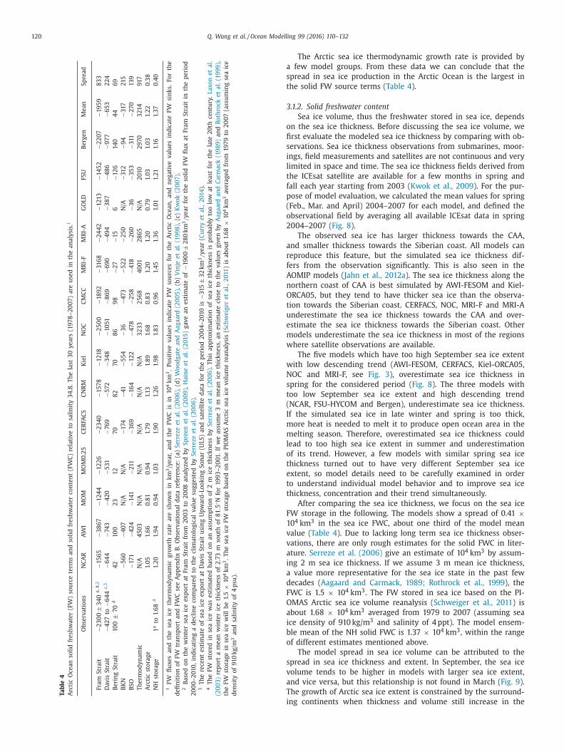
.1.1. Solid freshwater sources
In this section we assess the mean state of the source terms for
he Arctic solid FW, that is, the solid FW fluxes through the Arc-
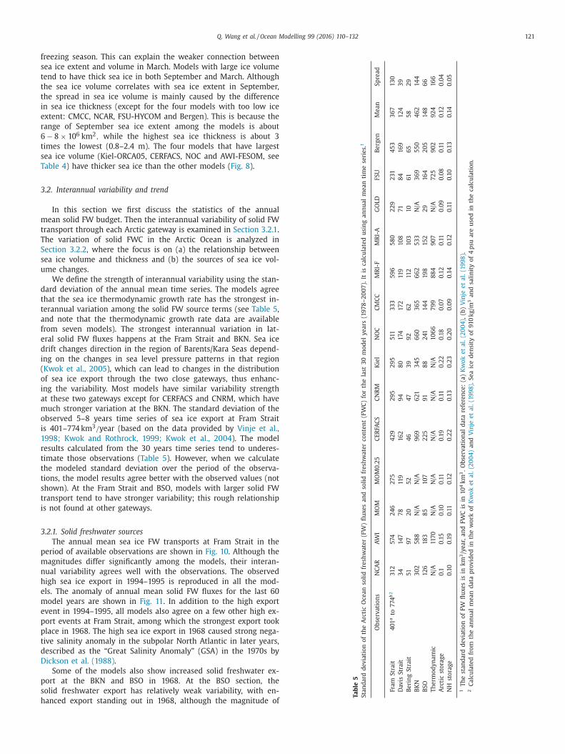
ic gateways and the sea ice thermodynamic growth rate. Table 4
hows the mean values of these diagnostics. In all the models solid
W fluxes through the gateways are the largest at Fram Strait.
owever, the solid FW fluxes have a big range among the mod-
ls. At Fram Strait, the spread in the simulated solid FW flux
s 810 km3/year, about one third of the synthesized mean value
−2300 ± 340 km3/year, Serreze et al. (2006)). Four models ob-
ained Fram Strait solid FW fluxes within the uncertainty range of
he synthesized value, including CERFACS, NOC, MRI-A and Bergen.
olid FW transport contains contributions from both sea ice and
now fluxes. It is found that the Fram Strait sea ice and snow fluxes
re well correlated in terms of interannual variability, and that sea
ce flux is the major contributor to the mean solid FW transport
accounting for more than 90% on average).
Sea ice FW flux depends on both sea ice thickness and drift
elocity (see Appendix B for the definition of sea ice FW flux). Kiel-
RCA05 is one of the models with the thickest sea ice, but it has
ery low Fram Strait solid FW export; The Bergen model has too
hin sea ice compared to the observation, but its Fram Strait solid
W export is close to the observed value. This indicates that the
delity of simulated sea ice flux does not reflect the model skills
n representing sea ice thickness and velocity. We will assess the
rctic sea ice thickness in Section 3.1.2.
The observed net solid FW flux at Davis Strait is toward the
abrador Sea (Kwok, 2007; Curry et al., 2014), and this direction is
eproduced in all the models (Table 4). The largest export flux is
ound in NOC and Bergen, with about twice the observed value. A
mall amount of solid FW is imported to the Arctic Ocean through
ering Strait according to observations (Woodgate and Aagaard,
005), but three models obtained (small) export fluxes, including
RI-F, MRI-A and Bergen.6
The models agree that Arctic sea ice is exported at the BKN
hen averaged over the last 30 years, and the Barents Sea has
et sea ice export through the BSO. In some models the amount
f solid FW flux entering Barents/Kara Seas from the north is
ery similar to that leaving at the BSO, while some models have
istinguishable difference between the two fluxes. NCAR, CERFACS,
NRM and Kiel-ORCA05 have larger fluxes at the BKN, but NOC
nd Bergen have larger outflow at the BSO. This means that there
s no agreement in the models on whether the Barents/Kara Seas
re a region of sink or source for sea ice.
6 The sea ice transport at Bering Strait is very small compared to other Arctic
ateways, so the model bias at this gateway has small impact on the total Arc-
ic FW budget. In this paper we show the results for all major Arctic gateways for
ompleteness. Quantifying impacts of model biases and their significance is not pur-
ued.
120 Q. Wang et al. / Ocean Modelling 99 (2016) 110–132
Ta
ble
4
Arc
tic
Oce
an
soli
dfr
esh
wa
ter
(FW
)so
urc
ete
rms
an
dso
lid
fre
shw
ate
rco
nte
nt
(FW
C)
rela
tiv
eto
sali
nit
y3
4.8
.T
he
last
30
ye
ars
(19
78
–2
00
7)
are
use
din
the
an
aly
sis.
1
Ob
serv
ati
on
sN
CA
RA
WI
MO
MM
OM
0.2
5C
ER
FAC
SC
NR
MK
iel
NO
CC
MC
CM
RI-
FM
RI-
AG
OLD
FS
UB
erg
en
Me
an
Sp
rea
d
Fra
mS
tra
it−2
30
0±
34
0a
,b
,2−1
56
5−3
86
7−1
24
4−1
22
6−2
34
0−1
57
8−1
21
8−2
50
0−1
89
2−3
16
8−2
44
2−1
21
3−1
45
2−2
20
7−1
95
98
33
Dav
isS
tra
it−4
27
to−6
44
c,3
−64
4−7
43
−42
0−5
31
−76
9−5
72
−34
8−1
05
1−8
69
−69
0−4
94
−38
7−4
86
−97
7−6
53
22
4
Be
rin
gS
tra
it1
00
±7
0d
42
10
02
31
27
08
27
08
69
8−2
7−1
56
−12
61
40
44
69
BK
N−5
60
−40
7N
/AN
/A−1
74
−41
−55
4−3
6−4
73
−52
2−2
50
N/A
−31
2−9
4−3
172
15
BS
O−1
71
−42
4−1
41
−211
−36
9−1
64
−12
2−4
78
−25
8−4
18
−26
0−3
6−3
53
−311
−27
01
39
Th
erm
od
yn
am
icN
/A4
50
3N
/AN
/AN
/AN
/AN
/A3
23
32
56
84
00
12
86
5N
/A2
01
02
97
03
21
49
17
Arc
tic
sto
rag
e1.
05
1.6
60
.81
0.9
41.
79
1.1
31.
89
1.6
80
.83
1.2
01.
20
0.7
91.
03
1.0
31.
22
0.3
8
NH
sto
rag
e1
ato
1.6
84
1.2
01.
94
0.9
41.
03
1.9
01.
26
1.9
81.
83
0.9
61.
45
1.3
61.
01
1.2
11.
16
1.3
70
.40
1F
Wfl
ux
es
an
dth
ese
aic
eth
erm
od
yn
am
icg
row
thra
tea
resh
ow
nin
km
3/y
ea
r,a
nd
the
FW
Cis
in1
04
km
3.
Po
siti
ve
va
lue
sin
dic
ate
FW
sou
rce
sfo
rth
eA
rcti
cO
cea
n,
an
dn
eg
ati
ve
va
lue
sin
dic
ate
FW
sin
ks.
For
the
de
fin
itio
no
fF
Wtr
an
spo
rta
nd
FW
Cse
eA
pp
en
dix
B.
Ob
serv
ati
on
al
da
tare
fere
nce
:(a
)S
err
eze
et
al.
(20
06
),(d
)W
oo
dg
ate
an
dA
ag
aa
rd(2
00
5),
(b)
Vin
jee
ta
l.(1
99
8),
(c)
Kw
ok
(20
07
).2
Ba
sed
on
the
win
ter
sea
ice
ex
po
rta
tFr
am
Str
ait
fro
m2
00
3to
20
08
an
aly
zed
by
Sp
ree
ne
ta
l.(2
00
9),
Ha
ine
et
al.
(20
15
)g
ave
an
est
ima
teo
f−1
90
0±
28
0k
m3/y
ea
rfo
rth
eso
lid
FW
flu
xa
tFr
am
Str
ait
inth
ep
eri
od
20
00
–2
01
0,
ind
ica
tin
ga
de
clin
eco
mp
are
dto
the
clim
ato
log
ica
lv
alu
esu
gg
est
ed
by
Se
rre
zee
ta
l.(2
00
6).
3T
he
rece
nt
est
ima
teo
fse
aic
ee
xp
ort
at
Dav
isS
tra
itu
sin
gU
pw
ard
-Lo
ok
ing
So
na
r(U
LS
)a
nd
sate
llit
ed
ata
for
the
pe
rio
d2
00
4–
20
10
is−3
15
±3
2k
m3/y
ea
r(C
urr
ye
ta
l.,
20
14
).4
Th
eF
Wst
ore
din
sea
ice
wa
se
stim
ate
db
ase
do
na
na
ssu
mp
tio
no
f2
mic
eth
ick
ne
ssb
yS
err
eze
et
al.
(20
06
).T
his
ap
pro
xim
ati
on
of
sea
ice
thic
kn
ess
isp
rob
ab
lyto
olo
wa
tle
ast
for
the
late
20
thce
ntu
ry.
Lax
on
et
al.
(20
03
)re
po
rta
me
an
win
ter
ice
thic
kn
ess
of
2.7
3m
sou
tho
f8
1.5
◦ Nfo
r1
99
3–
20
01.
Ifw
ea
ssu
me
3m
me
an
ice
thic
kn
ess
,a
ne
stim
ate
clo
seto
the
va
lue
sg
ive
nb
yA
ag
aa
rda
nd
Ca
rma
ck(1
98
9)
an
dR
oth
rock
et
al.
(19
99
),
the
FW
sto
rag
ein
sea
ice
wil
lb
e1.
5×
10
4k
m3.
Th
ese
aic
eF
Wst
ora
ge
ba
sed
on
the
PIO
MA
SA
rcti
cse
aic
ev
olu
me
rea
na
lysi
s(S
chw
eig
er
et
al.
,2
011
)is
ab
ou
t1.
68
×1
04
km
3av
era
ge
dfr
om
19
79
to2
00
7(a
ssu
min
gse
aic
e
de
nsi
tyo
f9
10
kg
/m3
an
dsa
lin
ity
of
4p
su).
a
s
t
3
o
fi
s
i
l
t
f
p
(
o
2
a
r
f
A
n
O
t
u
e
m
w
w
N
s
t
(
I
m
m
l
o
t
e
t
t
F
1
v
v
a
i
a
d
F
O
a
i
b
o
s
v
a
T
i
The Arctic sea ice thermodynamic growth rate is provided by
few model groups. From these data we can conclude that the
pread in sea ice production in the Arctic Ocean is the largest in
he solid FW source terms (Table 4).
.1.2. Solid freshwater content
Sea ice volume, thus the freshwater stored in sea ice, depends
n the sea ice thickness. Before discussing the sea ice volume, we
rst evaluate the modeled sea ice thickness by comparing with ob-
ervations. Sea ice thickness observations from submarines, moor-
ngs, field measurements and satellites are not continuous and very
imited in space and time. The sea ice thickness fields derived from
he ICEsat satellite are available for a few months in spring and
all each year starting from 2003 (Kwok et al., 2009). For the pur-
ose of model evaluation, we calculated the mean values for spring
Feb., Mar. and April) 2004–2007 for each model, and defined the
bservational field by averaging all available ICEsat data in spring
004–2007 (Fig. 8).
The observed sea ice has larger thickness towards the CAA,
nd smaller thickness towards the Siberian coast. All models can
eproduce this feature, but the simulated sea ice thickness dif-
ers from the observation significantly. This is also seen in the
OMIP models (Jahn et al., 2012a). The sea ice thickness along the
orthern coast of CAA is best simulated by AWI-FESOM and Kiel-
RCA05, but they tend to have thicker sea ice than the observa-
ion towards the Siberian coast. CERFACS, NOC, MRI-F and MRI-A
nderestimate the sea ice thickness towards the CAA and over-
stimate the sea ice thickness towards the Siberian coast. Other
odels underestimate the sea ice thickness in most of the regions
here satellite observations are available.
The five models which have too high September sea ice extent
ith low descending trend (AWI-FESOM, CERFACS, Kiel-ORCA05,
OC and MRI-F, see Fig. 3), overestimate sea ice thickness in
pring for the considered period (Fig. 8). The three models with
oo low September sea ice extent and high descending trend
NCAR, FSU-HYCOM and Bergen), underestimate sea ice thickness.
f the simulated sea ice in late winter and spring is too thick,
ore heat is needed to melt it to produce open ocean area in the
elting season. Therefore, overestimated sea ice thickness could
ead to too high sea ice extent in summer and underestimation
f its trend. However, a few models with similar spring sea ice
hickness turned out to have very different September sea ice
xtent, so model details need to be carefully examined in order
o understand individual model behavior and to improve sea ice
hickness, concentration and their trend simultaneously.
After comparing the sea ice thickness, we focus on the sea ice
W storage in the following. The models show a spread of 0.41 ×04 km3 in the sea ice FWC, about one third of the model mean
alue (Table 4). Due to lacking long term sea ice thickness obser-
ations, there are only rough estimates for the solid FWC in liter-
ture. Serreze et al. (2006) give an estimate of 104 km3 by assum-
ng 2 m sea ice thickness. If we assume 3 m mean ice thickness,
value more representative for the sea ice state in the past few
ecades (Aagaard and Carmack, 1989; Rothrock et al., 1999), the
WC is 1.5 × 10⁴ km3. The FW stored in sea ice based on the PI-
MAS Arctic sea ice volume reanalysis (Schweiger et al., 2011) is
bout 1.68 × 10⁴ km3 averaged from 1979 to 2007 (assuming sea
ce density of 910 kg/m3 and salinity of 4 ppt). The model ensem-
le mean of the NH solid FWC is 1.37 × 10⁴ km3, within the range
f different estimates mentioned above.
The model spread in sea ice volume can be attributed to the
pread in sea ice thickness and extent. In September, the sea ice
olume tends to be higher in models with larger sea ice extent,
nd vice versa, but this relationship is not found in March (Fig. 9).
he growth of Arctic sea ice extent is constrained by the surround-
ng continents when thickness and volume still increase in the
Q. Wang et al. / Ocean Modelling 99 (2016) 110–132 121
f
s
t
t
t
i
e
r
6
t
s
T
3
m
t
T
S
s
u
d
t
t
a
f
e
d
i
(
o
i
a
m
o
i
1
r
t
t
t
s
t
i
3
p
m
n
h
e
m
e
p
p
t
d
D
p
s
h
Ta
ble
5
Sta
nd
ard
de
via
tio
no
fth
eA
rcti
cO
cea
nso
lid
fre
shw
ate
r(F
W)
flu
xe
sa
nd
soli
dfr
esh
wa
ter
con
ten
t(F
WC
)fo
rth
ela
st3
0m
od
el
ye
ars
(19
78
–2
00
7).
Itis
calc
ula
ted
usi
ng
an
nu
al
me
an
tim
ese
rie
s.1
Ob
serv
ati
on
sN
CA
RA
WI
MO
MM
OM
0.2
5C
ER
FAC
SC
NR
MK
iel
NO
CC
MC
CM
RI-
FM
RI-
AG
OLD
FS
UB
erg
en
Me
an
Sp
rea
d
Fra
mS
tra
it4
01
ato
77
4b
23
12
57
42
46
27
54
29
29
52
95
511
33
35
96
58
02
29
23
14
53
36
71
30
Dav
isS
tra
it3
41
47
78
119
16
29
48
017
417
211
91
08
71
84
16
91
24
39
Be
rin
gS
tra
it5
19
72
05
24
64
73
99
26
211
21
03
10
61
65
58
29
BK
N3
02
58
8N
/AN
/A9
69
62
13
45
66
03
65
66
25
33
N/A
36
95
50
46
21
44
BS
O1
26
18
38
51
07
22
59
18
82
41
14
41
98
15
22
91
64
20
51
48
66
Th
erm
od
yn
am
icN
/A11
70
N/A
N/A
N/A
N/A
N/A
10
66
79
98
84
90
7N
/A7
25
90
29
24
16
6
Arc
tic
sto
rag
e0
.10
.15
0.1
00
.11
0.1
90
.11
0.2
20
.18
0.0
70
.12
0.1
10
.09
0.0
80
.11
0.1
20
.04
NH
sto
rag
e0
.10
0.1
90
.11
0.1
20
.22
0.1
30
.23
0.2
00
.09
0.1
40
.12
0.1
10
.10
0.1
30
.14
0.0
5
1T
he
sta
nd
ard
de
via
tio
no
fF
Wfl
ux
es
isin
km
3/y
ea
r,a
nd
FW
Cis
in1
04
km
3.
Ob
serv
ati
on
al
da
tare
fere
nce
:(a
)K
wo
ke
ta
l.(2
00
4),
(b)
Vin
jee
ta
l.(1
99
8).
2C
alc
ula
ted
fro
mth
ea
nn
ua
lm
ea
nd
ata
pro
vid
ed
inth
ew
ork
of
Kw
ok
et
al.
(20
04
)a
nd
Vin
jee
ta
l.(1
99
8).
Se
aic
ed
en
sity
of
91
0k
g/m
3a
nd
sali
nit
yo
f4
psu
are
use
din
the
calc
ula
tio
n.
reezing season. This can explain the weaker connection between
ea ice extent and volume in March. Models with large ice volume
end to have thick sea ice in both September and March. Although
he sea ice volume correlates with sea ice extent in September,
he spread in sea ice volume is mainly caused by the difference
n sea ice thickness (except for the four models with too low ice
xtent: CMCC, NCAR, FSU-HYCOM and Bergen). This is because the
ange of September sea ice extent among the models is about
− 8 × 10⁶ km2, while the highest sea ice thickness is about 3
imes the lowest (0.8–2.4 m). The four models that have largest
ea ice volume (Kiel-ORCA05, CERFACS, NOC and AWI-FESOM, see
able 4) have thicker sea ice than the other models (Fig. 8).
.2. Interannual variability and trend
In this section we first discuss the statistics of the annual
ean solid FW budget. Then the interannual variability of solid FW
ransport through each Arctic gateway is examined in Section 3.2.1.
he variation of solid FWC in the Arctic Ocean is analyzed in
ection 3.2.2, where the focus is on (a) the relationship between
ea ice volume and thickness and (b) the sources of sea ice vol-
me changes.
We define the strength of interannual variability using the stan-
ard deviation of the annual mean time series. The models agree
hat the sea ice thermodynamic growth rate has the strongest in-
erannual variation among the solid FW source terms (see Table 5,
nd note that the thermodynamic growth rate data are available
rom seven models). The strongest interannual variation in lat-
ral solid FW fluxes happens at the Fram Strait and BKN. Sea ice
rift changes direction in the region of Barents/Kara Seas depend-
ng on the changes in sea level pressure patterns in that region
Kwok et al., 2005), which can lead to changes in the distribution
f sea ice export through the two close gateways, thus enhanc-
ng the variability. Most models have similar variability strength
t these two gateways except for CERFACS and CNRM, which have
uch stronger variation at the BKN. The standard deviation of the
bserved 5–8 years time series of sea ice export at Fram Strait
s 401–774 km3/year (based on the data provided by Vinje et al.,
998; Kwok and Rothrock, 1999; Kwok et al., 2004). The model
esults calculated from the 30 years time series tend to underes-
imate those observations (Table 5). However, when we calculate
he modeled standard deviation over the period of the observa-
ions, the model results agree better with the observed values (not
hown). At the Fram Strait and BSO, models with larger solid FW
ransport tend to have stronger variability; this rough relationship
s not found at other gateways.
.2.1. Solid freshwater sources
The annual mean sea ice FW transports at Fram Strait in the
eriod of available observations are shown in Fig. 10. Although the
agnitudes differ significantly among the models, their interan-
ual variability agrees well with the observations. The observed
igh sea ice export in 1994–1995 is reproduced in all the mod-
ls. The anomaly of annual mean solid FW fluxes for the last 60
odel years are shown in Fig. 11. In addition to the high export
vent in 1994–1995, all models also agree on a few other high ex-
ort events at Fram Strait, among which the strongest export took
lace in 1968. The high sea ice export in 1968 caused strong nega-
ive salinity anomaly in the subpolar North Atlantic in later years,
escribed as the “Great Salinity Anomaly” (GSA) in the 1970s by
ickson et al. (1988).
Some of the models also show increased solid freshwater ex-
ort at the BKN and BSO in 1968. At the BSO section, the
olid freshwater export has relatively weak variability, with en-
anced export standing out in 1968, although the magnitude of
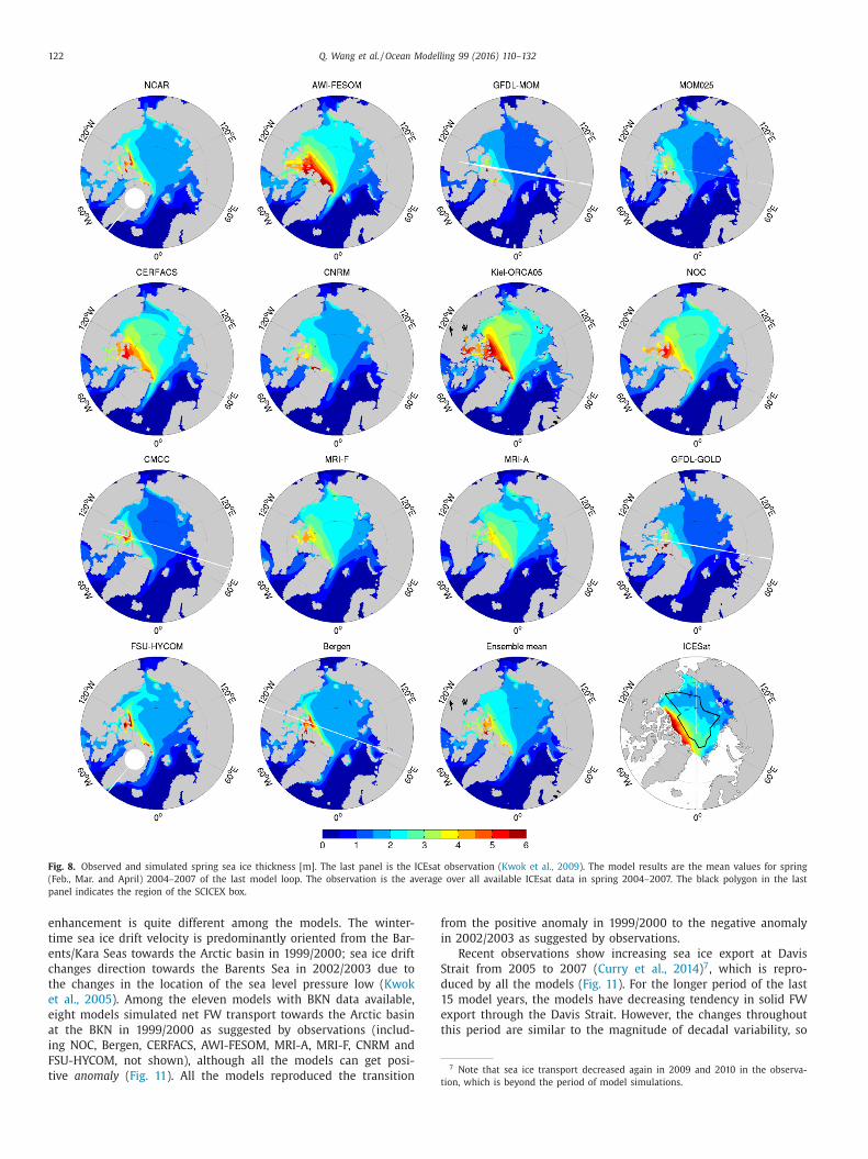
122 Q. Wang et al. / Ocean Modelling 99 (2016) 110–132
Fig. 8. Observed and simulated spring sea ice thickness [m]. The last panel is the ICEsat observation (Kwok et al., 2009). The model results are the mean values for spring
(Feb., Mar. and April) 2004–2007 of the last model loop. The observation is the average over all available ICEsat data in spring 2004–2007. The black polygon in the last
panel indicates the region of the SCICEX box.
f
i
S
d
1
e
t
7 Note that sea ice transport decreased again in 2009 and 2010 in the observa-
enhancement is quite different among the models. The winter-
time sea ice drift velocity is predominantly oriented from the Bar-
ents/Kara Seas towards the Arctic basin in 1999/2000; sea ice drift
changes direction towards the Barents Sea in 2002/2003 due to
the changes in the location of the sea level pressure low (Kwok
et al., 2005). Among the eleven models with BKN data available,
eight models simulated net FW transport towards the Arctic basin
at the BKN in 1999/2000 as suggested by observations (includ-
ing NOC, Bergen, CERFACS, AWI-FESOM, MRI-A, MRI-F, CNRM and
FSU-HYCOM, not shown), although all the models can get posi-
tive anomaly (Fig. 11). All the models reproduced the transition
trom the positive anomaly in 1999/2000 to the negative anomaly
n 2002/2003 as suggested by observations.
Recent observations show increasing sea ice export at Davis
trait from 2005 to 2007 (Curry et al., 2014)7, which is repro-
uced by all the models (Fig. 11). For the longer period of the last
5 model years, the models have decreasing tendency in solid FW
xport through the Davis Strait. However, the changes throughout
his period are similar to the magnitude of decadal variability, so
ion, which is beyond the period of model simulations.
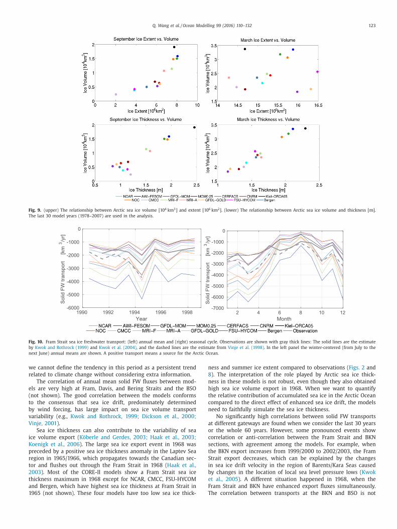
Q. Wang et al. / Ocean Modelling 99 (2016) 110–132 123
Fig. 9. (upper) The relationship between Arctic sea ice volume [104 km3] and extent [106 km2]. (lower) The relationship between Arctic sea ice volume and thickness [m].
The last 30 model years (1978–2007) are used in the analysis.
Year
1990 1992 1994 1996 1998
So
lid F
W tra
nsp
ort
[k
m3/y
r]
-6000
-5000
-4000
-3000
-2000
-1000
0
Month
2 4 6 8 10 12
Solid
FW
tra
nsport
[k
m3/y
r]
-7000
-6000
-5000
-4000
-3000
-2000
-1000
0
Fig. 10. Fram Strait sea ice freshwater transport: (left) annual mean and (right) seasonal cycle. Observations are shown with gray thick lines: The solid lines are the estimate
by Kwok and Rothrock (1999) and Kwok et al. (2004), and the dashed lines are the estimate from Vinje et al. (1998). In the left panel the winter-centered (from July to the
next June) annual means are shown. A positive transport means a source for the Arctic Ocean.
w
r
e
(
t
b
v
V
i
K
p
r
t
2
t
a
1
n
8
n
h
t
c
n
a
o
c
s
t
S
i
b
e
F
T
e cannot define the tendency in this period as a persistent trend
elated to climate change without considering extra information.
The correlation of annual mean solid FW fluxes between mod-
ls are very high at Fram, Davis, and Bering Straits and the BSO
not shown). The good correlation between the models conforms
o the consensus that sea ice drift, predominately determined
y wind forcing, has large impact on sea ice volume transport
ariability (e.g., Kwok and Rothrock, 1999; Dickson et al., 2000;
inje, 2001).
Sea ice thickness can also contribute to the variability of sea
ce volume export (Köberle and Gerdes, 2003; Haak et al., 2003;
oenigk et al., 2006). The large sea ice export event in 1968 was
receded by a positive sea ice thickness anomaly in the Laptev Sea
egion in 1965/1966, which propagates towards the Canadian sec-
or and flushes out through the Fram Strait in 1968 (Haak et al.,
003). Most of the CORE-II models show a Fram Strait sea ice
hickness maximum in 1968 except for NCAR, CMCC, FSU-HYCOM
nd Bergen, which have highest sea ice thickness at Fram Strait in
965 (not shown). These four models have too low sea ice thick-
ess and summer ice extent compared to observations (Figs. 2 and
). The interpretation of the role played by Arctic sea ice thick-
ess in these models is not robust, even though they also obtained
igh sea ice volume export in 1968. When we want to quantify
he relative contribution of accumulated sea ice in the Arctic Ocean
ompared to the direct effect of enhanced sea ice drift, the models
eed to faithfully simulate the sea ice thickness.
No significantly high correlations between solid FW transports
t different gateways are found when we consider the last 30 years
r the whole 60 years. However, some pronounced events show
orrelation or anti-correlation between the Fram Strait and BKN
ections, with agreement among the models. For example, when
he BKN export increases from 1999/2000 to 2002/2003, the Fram
trait export decreases, which can be explained by the changes
n sea ice drift velocity in the region of Barents/Kara Seas caused
y changes in the location of local sea level pressure lows (Kwok
t al., 2005). A different situation happened in 1968, when the
ram Strait and BKN have enhanced export fluxes simultaneously.
he correlation between transports at the BKN and BSO is not
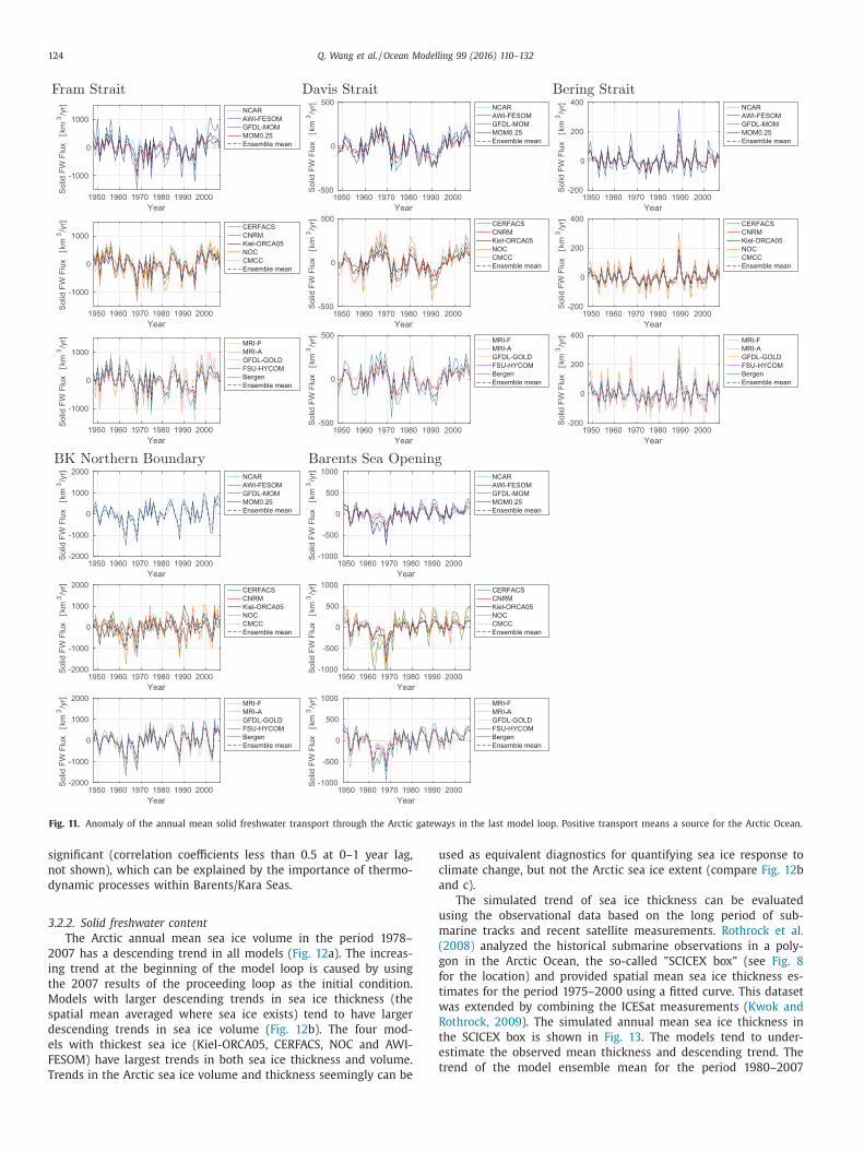
124 Q. Wang et al. / Ocean Modelling 99 (2016) 110–132
tiartSgnireBtiartSsivaDtiartSmarF
Year
1950 1960 1970 1980 1990 2000
Solid
FW
Flu
x
[km
3/y
r]
-1000
0
1000
NCAR
AWI-FESOM
GFDL-MOM
MOM0.25
Ensemble mean
Year
1950 1960 1970 1980 1990 2000
Solid
FW
Flu
x
[km
3/y
r]
-500
0
500NCAR
AWI-FESOM
GFDL-MOM
MOM0.25
Ensemble mean
Year
1950 1960 1970 1980 1990 2000
Solid
FW
Flu
x
[km
3/y
r]
-200
0
200
400NCAR
AWI-FESOM
GFDL-MOM
MOM0.25
Ensemble mean
Year
1950 1960 1970 1980 1990 2000
Solid
FW
Flu
x
[km
3/y
r]
-1000
0
1000
CERFACS
CNRM
Kiel-ORCA05
NOC
CMCC
Ensemble mean
Year
1950 1960 1970 1980 1990 2000S
olid
FW
Flu
x
[km
3/y
r]-500
0
500CERFACS
CNRM
Kiel-ORCA05
NOC
CMCC
Ensemble mean
Year
1950 1960 1970 1980 1990 2000
Solid
FW
Flu
x
[km
3/y
r]
-200
0
200
400CERFACS
CNRM
Kiel-ORCA05
NOC
CMCC
Ensemble mean
Year
1950 1960 1970 1980 1990 2000
Solid
FW
Flu
x
[km
3/y
r]
-1000
0
1000
MRI-F
MRI-A
GFDL-GOLD
FSU-HYCOM
Bergen
Ensemble mean
Year
1950 1960 1970 1980 1990 2000
Solid
FW
Flu
x
[km
3/y
r]
-500
0
500MRI-F
MRI-A
GFDL-GOLD
FSU-HYCOM
Bergen
Ensemble mean
Year
1950 1960 1970 1980 1990 2000
Solid
FW
Flu
x
[km
3/y
r]
-200
0
200
400MRI-F
MRI-A
GFDL-GOLD
FSU-HYCOM
Bergen
Ensemble mean
BK Northern Boundary Barents Sea Opening
Year
1950 1960 1970 1980 1990 2000
Solid
FW
Flu
x
[km
3/y
r]
-2000
-1000
0
1000
2000NCAR
AWI-FESOM
GFDL-MOM
MOM0.25
Ensemble mean
Year
1950 1960 1970 1980 1990 2000
Solid
FW
Flu
x
[km
3/y
r]
-1000
-500
0
500
1000NCAR
AWI-FESOM
GFDL-MOM
MOM0.25
Ensemble mean
Year
1950 1960 1970 1980 1990 2000
Solid
FW
Flu
x
[km
3/y
r]
-2000
-1000
0
1000
2000CERFACS
CNRM
Kiel-ORCA05
NOC
CMCC
Ensemble mean
Year
1950 1960 1970 1980 1990 2000
Solid
FW
Flu
x
[km
3/y
r]
-1000
-500
0
500
1000CERFACS
CNRM
Kiel-ORCA05
NOC
CMCC
Ensemble mean
Year
1950 1960 1970 1980 1990 2000
Solid
FW
Flu
x
[km
3/y
r]
-2000
-1000
0
1000
2000MRI-F
MRI-A
GFDL-GOLD
FSU-HYCOM
Bergen
Ensemble mean
Year
1950 1960 1970 1980 1990 2000
Solid
FW
Flu
x
[km
3/y
r]
-1000
-500
0
500
1000MRI-F
MRI-A
GFDL-GOLD
FSU-HYCOM
Bergen
Ensemble mean
Fig. 11. Anomaly of the annual mean solid freshwater transport through the Arctic gateways in the last model loop. Positive transport means a source for the Arctic Ocean.
u
c
a
u
m
(
g
f
t
w
R
t
e
t
significant (correlation coefficients less than 0.5 at 0–1 year lag,
not shown), which can be explained by the importance of thermo-
dynamic processes within Barents/Kara Seas.
3.2.2. Solid freshwater content
The Arctic annual mean sea ice volume in the period 1978–
2007 has a descending trend in all models (Fig. 12a). The increas-
ing trend at the beginning of the model loop is caused by using
the 2007 results of the proceeding loop as the initial condition.
Models with larger descending trends in sea ice thickness (the
spatial mean averaged where sea ice exists) tend to have larger
descending trends in sea ice volume (Fig. 12b). The four mod-
els with thickest sea ice (Kiel-ORCA05, CERFACS, NOC and AWI-
FESOM) have largest trends in both sea ice thickness and volume.
Trends in the Arctic sea ice volume and thickness seemingly can be
sed as equivalent diagnostics for quantifying sea ice response to
limate change, but not the Arctic sea ice extent (compare Fig. 12b
nd c).
The simulated trend of sea ice thickness can be evaluated
sing the observational data based on the long period of sub-
arine tracks and recent satellite measurements. Rothrock et al.
2008) analyzed the historical submarine observations in a poly-
on in the Arctic Ocean, the so-called ”SCICEX box” (see Fig. 8
or the location) and provided spatial mean sea ice thickness es-
imates for the period 1975–2000 using a fitted curve. This dataset
as extended by combining the ICESat measurements (Kwok and
othrock, 2009). The simulated annual mean sea ice thickness in
he SCICEX box is shown in Fig. 13. The models tend to under-
stimate the observed mean thickness and descending trend. The
rend of the model ensemble mean for the period 1980–2007
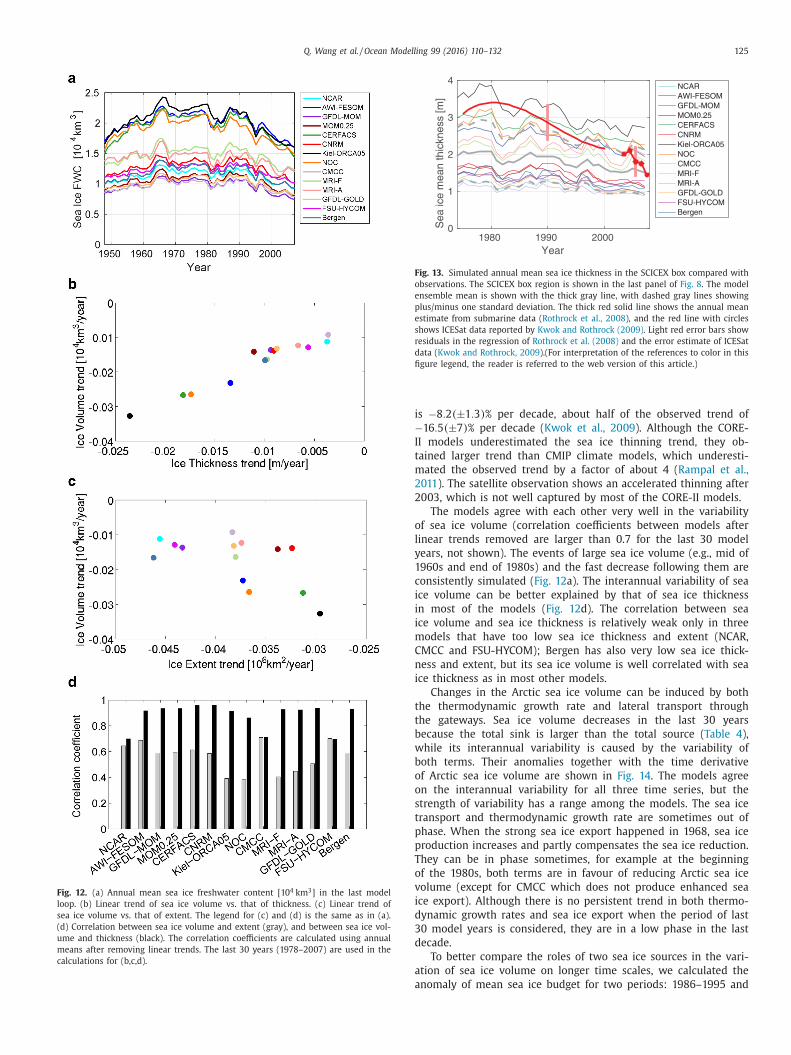
Q. Wang et al. / Ocean Modelling 99 (2016) 110–132 125
Fig. 12. (a) Annual mean sea ice freshwater content [104 km3] in the last model
loop. (b) Linear trend of sea ice volume vs. that of thickness. (c) Linear trend of
sea ice volume vs. that of extent. The legend for (c) and (d) is the same as in (a).
(d) Correlation between sea ice volume and extent (gray), and between sea ice vol-
ume and thickness (black). The correlation coefficients are calculated using annual
means after removing linear trends. The last 30 years (1978–2007) are used in the
calculations for (b,c,d).
Year1980 1990 2000
Sea
ice
mea
n th
ickn
ess
[m]
0
1
2
3
4NCARAWI-FESOMGFDL-MOMMOM0.25CERFACSCNRMKiel-ORCA05NOCCMCCMRI-FMRI-AGFDL-GOLDFSU-HYCOMBergen
Fig. 13. Simulated annual mean sea ice thickness in the SCICEX box compared with
observations. The SCICEX box region is shown in the last panel of Fig. 8. The model
ensemble mean is shown with the thick gray line, with dashed gray lines showing
plus/minus one standard deviation. The thick red solid line shows the annual mean
estimate from submarine data (Rothrock et al., 2008), and the red line with circles
shows ICESat data reported by Kwok and Rothrock (2009). Light red error bars show
residuals in the regression of Rothrock et al. (2008) and the error estimate of ICESat
data (Kwok and Rothrock, 2009).(For interpretation of the references to color in this
figure legend, the reader is referred to the web version of this article.)
i
−I
t
m
2
2
o
l
y
1
c
i
i
i
m
C
n
i
t
t
b
w
b
o
o
s
t
p
p
T
o
v
i
d
3
d
a
a
s −8.2(±1.3)% per decade, about half of the observed trend of
16.5(±7)% per decade (Kwok et al., 2009). Although the CORE-
I models underestimated the sea ice thinning trend, they ob-
ained larger trend than CMIP climate models, which underesti-
ated the observed trend by a factor of about 4 (Rampal et al.,
011). The satellite observation shows an accelerated thinning after
003, which is not well captured by most of the CORE-II models.
The models agree with each other very well in the variability
f sea ice volume (correlation coefficients between models after
inear trends removed are larger than 0.7 for the last 30 model
ears, not shown). The events of large sea ice volume (e.g., mid of
960s and end of 1980s) and the fast decrease following them are
onsistently simulated (Fig. 12a). The interannual variability of sea
ce volume can be better explained by that of sea ice thickness
n most of the models (Fig. 12d). The correlation between sea
ce volume and sea ice thickness is relatively weak only in three
odels that have too low sea ice thickness and extent (NCAR,
MCC and FSU-HYCOM); Bergen has also very low sea ice thick-
ess and extent, but its sea ice volume is well correlated with sea
ce thickness as in most other models.
Changes in the Arctic sea ice volume can be induced by both
he thermodynamic growth rate and lateral transport through
he gateways. Sea ice volume decreases in the last 30 years
ecause the total sink is larger than the total source (Table 4),
hile its interannual variability is caused by the variability of
oth terms. Their anomalies together with the time derivative
f Arctic sea ice volume are shown in Fig. 14. The models agree
n the interannual variability for all three time series, but the
trength of variability has a range among the models. The sea ice
ransport and thermodynamic growth rate are sometimes out of
hase. When the strong sea ice export happened in 1968, sea ice
roduction increases and partly compensates the sea ice reduction.
hey can be in phase sometimes, for example at the beginning
f the 1980s, both terms are in favour of reducing Arctic sea ice
olume (except for CMCC which does not produce enhanced sea
ce export). Although there is no persistent trend in both thermo-
ynamic growth rates and sea ice export when the period of last
0 model years is considered, they are in a low phase in the last
ecade.
To better compare the roles of two sea ice sources in the vari-
tion of sea ice volume on longer time scales, we calculated the
nomaly of mean sea ice budget for two periods: 1986–1995 and
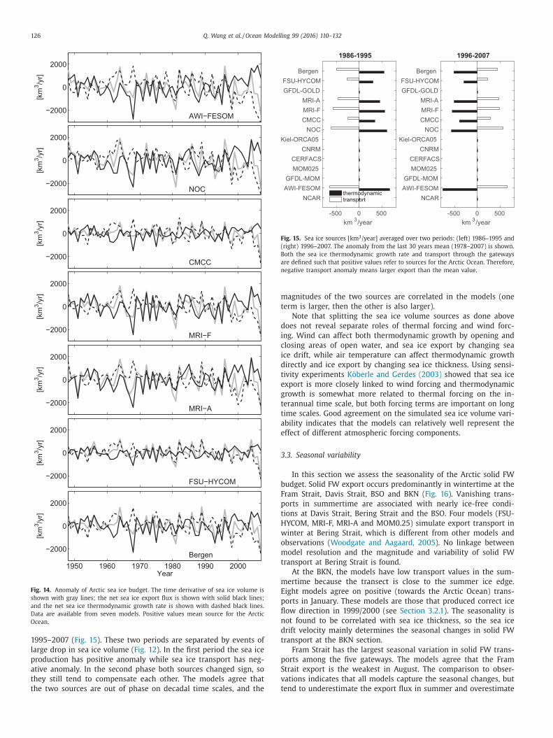
126 Q. Wang et al. / Ocean Modelling 99 (2016) 110–132
−2000
0
2000
[km
3/y
r]
AWI−FESOM
−2000
0
2000
[km
3/y
r]
NOC
−2000
0
2000
[km
3/y
r]
CMCC
−2000
0
2000
[km
3/y
r]
MRI−F
−2000
0
2000
[km
3/y
r]
MRI−A
−2000
0
2000
[km
3/y
r]
FSU−HYCOM
1950 1960 1970 1980 1990 2000
−2000
0
2000
Year
[km
3/y
r]
Bergen
Fig. 14. Anomaly of Arctic sea ice budget. The time derivative of sea ice volume is
shown with gray lines; the net sea ice export flux is shown with solid black lines;
and the net sea ice thermodynamic growth rate is shown with dashed black lines.
Data are available from seven models. Positive values mean source for the Arctic
Ocean.
km3/year
-500 0 500
NCAR
AWI-FESOM
GFDL-MOM
MOM025
CERFACS
CNRM
Kiel-ORCA05
NOC
CMCC
MRI-F
MRI-A
GFDL-GOLD
FSU-HYCOM
Bergen
1986-1995
thermodynamictransport
km3/year
-500 0 500
NCAR
AWI-FESOM
GFDL-MOM
MOM025
CERFACS
CNRM
Kiel-ORCA05
NOC
CMCC
MRI-F
MRI-A
GFDL-GOLD
FSU-HYCOM
Bergen
1996-2007
Fig. 15. Sea ice sources [km3/year] averaged over two periods: (left) 1986–1995 and
(right) 1996–2007. The anomaly from the last 30 years mean (1978–2007) is shown.
Both the sea ice thermodynamic growth rate and transport through the gateways
are defined such that positive values refer to sources for the Arctic Ocean. Therefore,
negative transport anomaly means larger export than the mean value.
m
t
d
i
c
i
d
t
e
g
t
t
a
e
3
b
F
p
t
H
w
o
m
t
m
E
p
fl
n
d
t
p
S
v
t
1995–2007 (Fig. 15). These two periods are separated by events of
large drop in sea ice volume (Fig. 12). In the first period the sea ice
production has positive anomaly while sea ice transport has neg-
ative anomaly. In the second phase both sources changed sign, so
they still tend to compensate each other. The models agree that
the two sources are out of phase on decadal time scales, and the
agnitudes of the two sources are correlated in the models (one
erm is larger, then the other is also larger).
Note that splitting the sea ice volume sources as done above
oes not reveal separate roles of thermal forcing and wind forc-
ng. Wind can affect both thermodynamic growth by opening and
losing areas of open water, and sea ice export by changing sea
ce drift, while air temperature can affect thermodynamic growth
irectly and ice export by changing sea ice thickness. Using sensi-
ivity experiments Köberle and Gerdes (2003) showed that sea ice
xport is more closely linked to wind forcing and thermodynamic
rowth is somewhat more related to thermal forcing on the in-
erannual time scale, but both forcing terms are important on long
ime scales. Good agreement on the simulated sea ice volume vari-
bility indicates that the models can relatively well represent the
ffect of different atmospheric forcing components.
.3. Seasonal variability
In this section we assess the seasonality of the Arctic solid FW
udget. Solid FW export occurs predominantly in wintertime at the
ram Strait, Davis Strait, BSO and BKN (Fig. 16). Vanishing trans-
orts in summertime are associated with nearly ice-free condi-
ions at Davis Strait, Bering Strait and the BSO. Four models (FSU-
YCOM, MRI-F, MRI-A and MOM0.25) simulate export transport in
inter at Bering Strait, which is different from other models and
bservations (Woodgate and Aagaard, 2005). No linkage between
odel resolution and the magnitude and variability of solid FW
ransport at Bering Strait is found.
At the BKN, the models have low transport values in the sum-
ertime because the transect is close to the summer ice edge.
ight models agree on positive (towards the Arctic Ocean) trans-
orts in January. These models are those that produced correct ice
ow direction in 1999/2000 (see Section 3.2.1). The seasonality is
ot found to be correlated with sea ice thickness, so the sea ice
rift velocity mainly determines the seasonal changes in solid FW
ransport at the BKN section.
Fram Strait has the largest seasonal variation in solid FW trans-
orts among the five gateways. The models agree that the Fram
trait export is the weakest in August. The comparison to obser-
ations indicates that all models capture the seasonal changes, but
end to underestimate the export flux in summer and overestimate
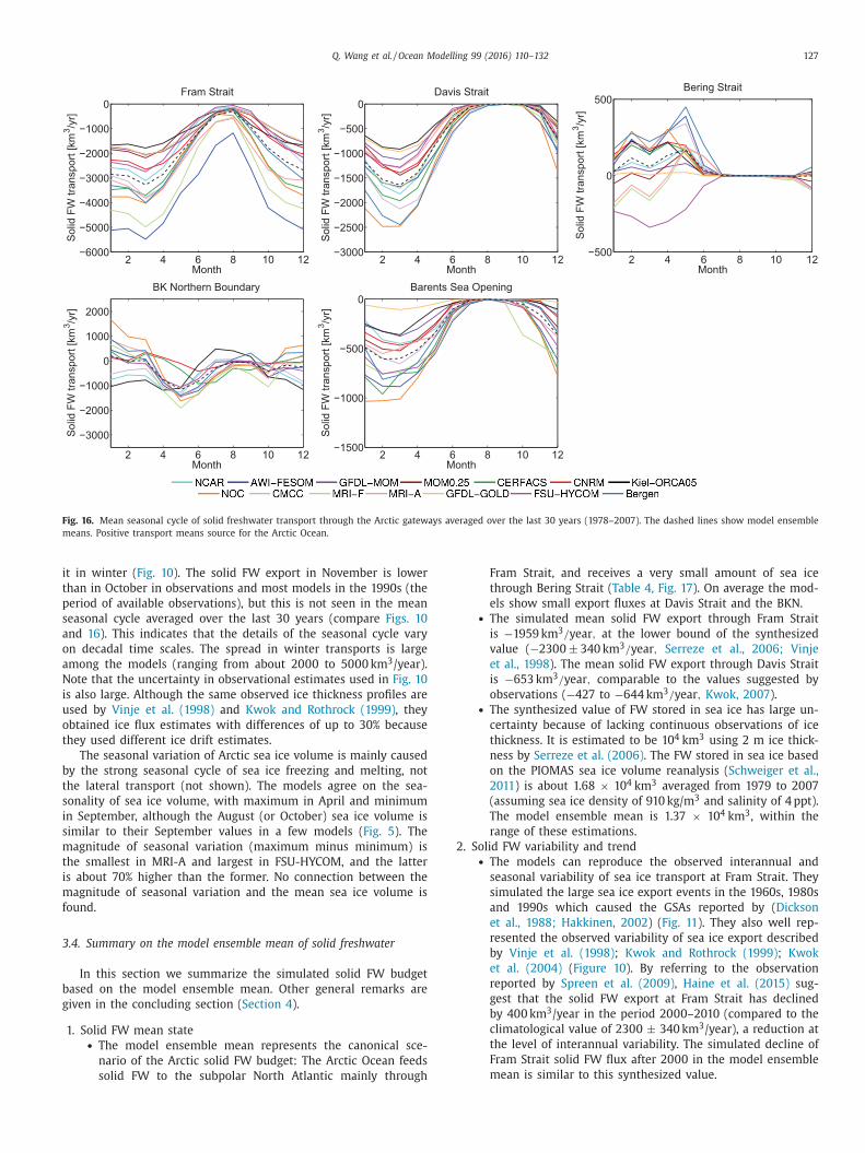
Q. Wang et al. / Ocean Modelling 99 (2016) 110–132 127
2 4 6 8 10 12−6000
−5000
−4000
−3000
−2000
−1000
0
Month
Solid
FW
tra
nsport
[km
3/y
r]
Fram Strait
2 4 6 8 10 12−3000
−2500
−2000
−1500
−1000
−500
0
Month
Solid
FW
tra
nsport
[km
3/y
r]
Davis Strait
2 4 6 8 10 12−500
0
500
Month
Solid
FW
tra
nsport
[km
3/y
r]
Bering Strait
2 4 6 8 10 12
−3000
−2000
−1000
0
1000
2000
Month
Solid
FW
tra
nsport
[km
3/y
r]
BK Northern Boundary
2 4 6 8 10 12−1500
−1000
−500
0
Month
Solid
FW
tra
nsport
[km
3/y
r]
Barents Sea Opening
Fig. 16. Mean seasonal cycle of solid freshwater transport through the Arctic gateways averaged over the last 30 years (1978–2007). The dashed lines show model ensemble
means. Positive transport means source for the Arctic Ocean.
i
t
p
s
a
o
a
N
i
u
o
t
b
t
s
i
s
m
t
i
m
f
3
b
g
t in winter (Fig. 10). The solid FW export in November is lower
han in October in observations and most models in the 1990s (the
eriod of available observations), but this is not seen in the mean
easonal cycle averaged over the last 30 years (compare Figs. 10
nd 16). This indicates that the details of the seasonal cycle vary
n decadal time scales. The spread in winter transports is large
mong the models (ranging from about 2000 to 5000 km3/year).
ote that the uncertainty in observational estimates used in Fig. 10
s also large. Although the same observed ice thickness profiles are
sed by Vinje et al. (1998) and Kwok and Rothrock (1999), they
btained ice flux estimates with differences of up to 30% because
hey used different ice drift estimates.
The seasonal variation of Arctic sea ice volume is mainly caused
y the strong seasonal cycle of sea ice freezing and melting, not
he lateral transport (not shown). The models agree on the sea-
onality of sea ice volume, with maximum in April and minimum
n September, although the August (or October) sea ice volume is
imilar to their September values in a few models (Fig. 5). The
agnitude of seasonal variation (maximum minus minimum) is
he smallest in MRI-A and largest in FSU-HYCOM, and the latter
s about 70% higher than the former. No connection between the
agnitude of seasonal variation and the mean sea ice volume is
ound.
.4. Summary on the model ensemble mean of solid freshwater
In this section we summarize the simulated solid FW budget
ased on the model ensemble mean. Other general remarks are
iven in the concluding section (Section 4).
1. Solid FW mean state• The model ensemble mean represents the canonical sce-
nario of the Arctic solid FW budget: The Arctic Ocean feeds
solid FW to the subpolar North Atlantic mainly through
Fram Strait, and receives a very small amount of sea ice
through Bering Strait (Table 4, Fig. 17). On average the mod-
els show small export fluxes at Davis Strait and the BKN.• The simulated mean solid FW export through Fram Strait
is −1959 km3/year, at the lower bound of the synthesized
value (−2300 ± 340 km3/year, Serreze et al., 2006; Vinje
et al., 1998). The mean solid FW export through Davis Strait
is −653 km3/year, comparable to the values suggested by
observations (−427 to −644 km3/year, Kwok, 2007).• The synthesized value of FW stored in sea ice has large un-
certainty because of lacking continuous observations of ice
thickness. It is estimated to be 104 km3 using 2 m ice thick-
ness by Serreze et al. (2006). The FW stored in sea ice based
on the PIOMAS sea ice volume reanalysis (Schweiger et al.,
2011) is about 1.68 × 10⁴ km3 averaged from 1979 to 2007
(assuming sea ice density of 910 kg/m3 and salinity of 4 ppt).
The model ensemble mean is 1.37 × 10⁴ km3, within the
range of these estimations.
2. Solid FW variability and trend• The models can reproduce the observed interannual and
seasonal variability of sea ice transport at Fram Strait. They
simulated the large sea ice export events in the 1960s, 1980s
and 1990s which caused the GSAs reported by (Dickson
et al., 1988; Hakkinen, 2002) (Fig. 11). They also well rep-
resented the observed variability of sea ice export described
by Vinje et al. (1998); Kwok and Rothrock (1999); Kwok
et al. (2004) (Figure 10). By referring to the observation
reported by Spreen et al. (2009), Haine et al. (2015) sug-
gest that the solid FW export at Fram Strait has declined
by 400 km3/year in the period 2000–2010 (compared to the
climatological value of 2300 ± 340 km3/year), a reduction at
the level of interannual variability. The simulated decline of
Fram Strait solid FW flux after 2000 in the model ensemble
mean is similar to this synthesized value.
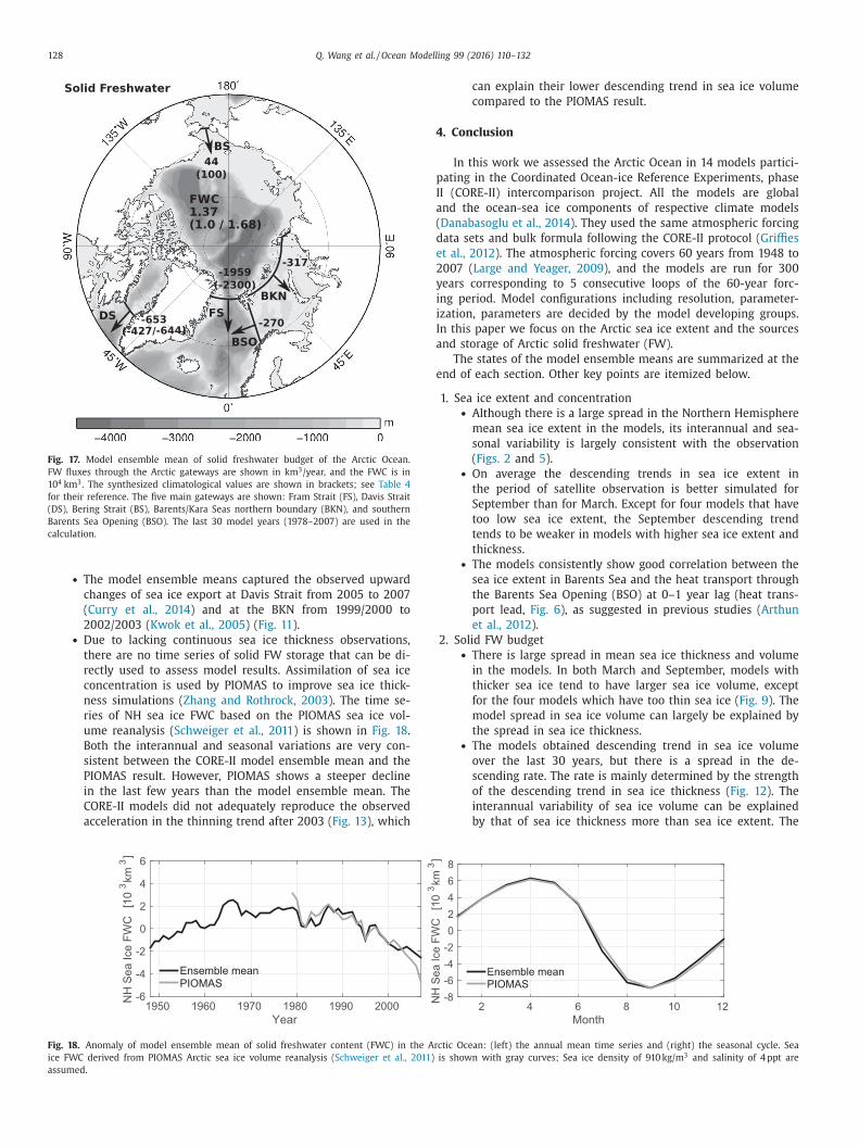
128 Q. Wang et al. / Ocean Modelling 99 (2016) 110–132
Fig. 17. Model ensemble mean of solid freshwater budget of the Arctic Ocean.
FW fluxes through the Arctic gateways are shown in km3/year, and the FWC is in
104 km3. The synthesized climatological values are shown in brackets; see Table 4
for their reference. The five main gateways are shown: Fram Strait (FS), Davis Strait
(DS), Bering Strait (BS), Barents/Kara Seas northern boundary (BKN), and southern
Barents Sea Opening (BSO). The last 30 model years (1978–2007) are used in the
calculation.
4
p
I
a
(
d
e
2
y
i
i
I
a
e
• The model ensemble means captured the observed upward
changes of sea ice export at Davis Strait from 2005 to 2007
(Curry et al., 2014) and at the BKN from 1999/2000 to
2002/2003 (Kwok et al., 2005) (Fig. 11).• Due to lacking continuous sea ice thickness observations,
there are no time series of solid FW storage that can be di-
rectly used to assess model results. Assimilation of sea ice
concentration is used by PIOMAS to improve sea ice thick-
ness simulations (Zhang and Rothrock, 2003). The time se-
ries of NH sea ice FWC based on the PIOMAS sea ice vol-
ume reanalysis (Schweiger et al., 2011) is shown in Fig. 18.
Both the interannual and seasonal variations are very con-
sistent between the CORE-II model ensemble mean and the
PIOMAS result. However, PIOMAS shows a steeper decline
in the last few years than the model ensemble mean. The
CORE-II models did not adequately reproduce the observed
acceleration in the thinning trend after 2003 (Fig. 13), which
Year1950 1960 1970 1980 1990 2000
NH
Sea Ice F
WC
[1
03km
3]
-6
-4
-2
0
2
4
6
Ensemble meanPIOMAS
33
Fig. 18. Anomaly of model ensemble mean of solid freshwater content (FWC) in the Ar
ice FWC derived from PIOMAS Arctic sea ice volume reanalysis (Schweiger et al., 2011)
assumed.
can explain their lower descending trend in sea ice volume
compared to the PIOMAS result.
. Conclusion
In this work we assessed the Arctic Ocean in 14 models partici-
ating in the Coordinated Ocean-ice Reference Experiments, phase
I (CORE-II) intercomparison project. All the models are global
nd the ocean-sea ice components of respective climate models
Danabasoglu et al., 2014). They used the same atmospheric forcing
ata sets and bulk formula following the CORE-II protocol (Griffies
t al., 2012). The atmospheric forcing covers 60 years from 1948 to
007 (Large and Yeager, 2009), and the models are run for 300
ears corresponding to 5 consecutive loops of the 60-year forc-
ng period. Model configurations including resolution, parameter-
zation, parameters are decided by the model developing groups.
n this paper we focus on the Arctic sea ice extent and the sources
nd storage of Arctic solid freshwater (FW).
The states of the model ensemble means are summarized at the
nd of each section. Other key points are itemized below.
1. Sea ice extent and concentration• Although there is a large spread in the Northern Hemisphere
mean sea ice extent in the models, its interannual and sea-
sonal variability is largely consistent with the observation
(Figs. 2 and 5).• On average the descending trends in sea ice extent in
the period of satellite observation is better simulated for
September than for March. Except for four models that have
too low sea ice extent, the September descending trend
tends to be weaker in models with higher sea ice extent and
thickness.• The models consistently show good correlation between the
sea ice extent in Barents Sea and the heat transport through
the Barents Sea Opening (BSO) at 0–1 year lag (heat trans-
port lead, Fig. 6), as suggested in previous studies (Arthun
et al., 2012).
2. Solid FW budget• There is large spread in mean sea ice thickness and volume
in the models. In both March and September, models with
thicker sea ice tend to have larger sea ice volume, except
for the four models which have too thin sea ice (Fig. 9). The
model spread in sea ice volume can largely be explained by
the spread in sea ice thickness.• The models obtained descending trend in sea ice volume
over the last 30 years, but there is a spread in the de-
scending rate. The rate is mainly determined by the strength
of the descending trend in sea ice thickness (Fig. 12). The
interannual variability of sea ice volume can be explained
by that of sea ice thickness more than sea ice extent. The
Month2 4 6 8 10 12
NH
Se
a Ice
FW
C
[10
km
]
-8
-6
-4
-2
0
2
4
6
8
Ensemble meanPIOMAS
ctic Ocean: (left) the annual mean time series and (right) the seasonal cycle. Sea
is shown with gray curves; Sea ice density of 910 kg/m3 and salinity of 4 ppt are
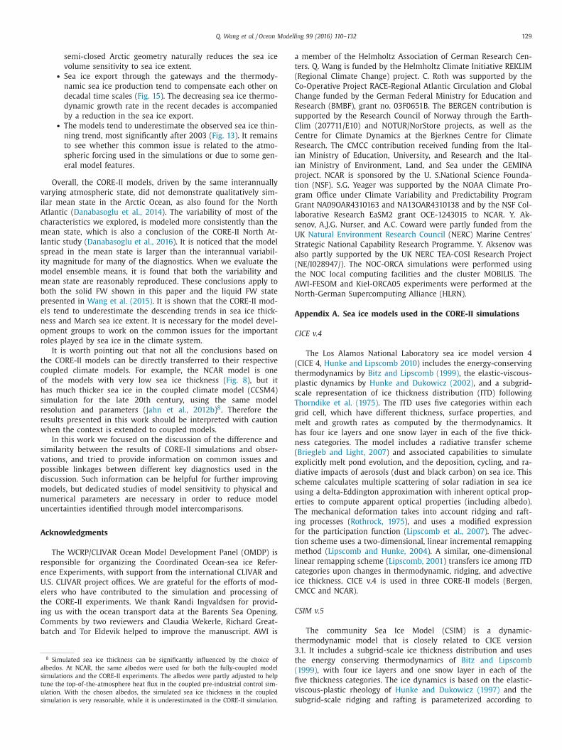
Q. Wang et al. / Ocean Modelling 99 (2016) 110–132 129
v
i
A
c
m
l
s
i
m
m
b
p
e
n
o
r
t
c
o
h
s
r
r
w
s
v
p
d
m
n
u
A
r
e
U
e
t
i
C
b
a
s
t
u
s
a
t
(
C
C
R
s
C
C
R
i
i
p
t
g
G
l
s
U
S
a
(
t
A
N
A
C
(
t
p
s
T
g
m
h
n
(
e
d
s
u
e
T
i
f
t
m
l
c
i
C
C
semi-closed Arctic geometry naturally reduces the sea ice
volume sensitivity to sea ice extent.• Sea ice export through the gateways and the thermody-
namic sea ice production tend to compensate each other on
decadal time scales (Fig. 15). The decreasing sea ice thermo-
dynamic growth rate in the recent decades is accompanied
by a reduction in the sea ice export.• The models tend to underestimate the observed sea ice thin-
ning trend, most significantly after 2003 (Fig. 13). It remains
to see whether this common issue is related to the atmo-
spheric forcing used in the simulations or due to some gen-
eral model features.
Overall, the CORE-II models, driven by the same interannually
arying atmospheric state, did not demonstrate qualitatively sim-
lar mean state in the Arctic Ocean, as also found for the North
tlantic (Danabasoglu et al., 2014). The variability of most of the
haracteristics we explored, is modeled more consistently than the
ean state, which is also a conclusion of the CORE-II North At-
antic study (Danabasoglu et al., 2016). It is noticed that the model
pread in the mean state is larger than the interannual variabil-
ty magnitude for many of the diagnostics. When we evaluate the
odel ensemble means, it is found that both the variability and
ean state are reasonably reproduced. These conclusions apply to
oth the solid FW shown in this paper and the liquid FW state
resented in Wang et al. (2015). It is shown that the CORE-II mod-
ls tend to underestimate the descending trends in sea ice thick-
ess and March sea ice extent. It is necessary for the model devel-
pment groups to work on the common issues for the important
oles played by sea ice in the climate system.
It is worth pointing out that not all the conclusions based on
he CORE-II models can be directly transferred to their respective
oupled climate models. For example, the NCAR model is one
f the models with very low sea ice thickness (Fig. 8), but it
as much thicker sea ice in the coupled climate model (CCSM4)
imulation for the late 20th century, using the same model
esolution and parameters (Jahn et al., 2012b)8. Therefore the
esults presented in this work should be interpreted with caution
hen the context is extended to coupled models.
In this work we focused on the discussion of the difference and
imilarity between the results of CORE-II simulations and obser-
ations, and tried to provide information on common issues and
ossible linkages between different key diagnostics used in the
iscussion. Such information can be helpful for further improving
odels, but dedicated studies of model sensitivity to physical and
umerical parameters are necessary in order to reduce model
ncertainties identified through model intercomparisons.
cknowledgments
The WCRP/CLIVAR Ocean Model Development Panel (OMDP) is
esponsible for organizing the Coordinated Ocean-sea ice Refer-
nce Experiments, with support from the international CLIVAR and
.S. CLIVAR project offices. We are grateful for the efforts of mod-
lers who have contributed to the simulation and processing of
he CORE-II experiments. We thank Randi Ingvaldsen for provid-
ng us with the ocean transport data at the Barents Sea Opening.
omments by two reviewers and Claudia Wekerle, Richard Great-
atch and Tor Eldevik helped to improve the manuscript. AWI is
8 Simulated sea ice thickness can be significantly influenced by the choice of
lbedos. At NCAR, the same albedos were used for both the fully-coupled model
imulations and the CORE-II experiments. The albedos were partly adjusted to help
une the top-of-the-atmosphere heat flux in the coupled pre-industrial control sim-
lation. With the chosen albedos, the simulated sea ice thickness in the coupled
imulation is very reasonable, while it is underestimated in the CORE-II simulation.
t
3
t
(
fi
v
s
member of the Helmholtz Association of German Research Cen-
ers. Q. Wang is funded by the Helmholtz Climate Initiative REKLIM
Regional Climate Change) project. C. Roth was supported by the
o-Operative Project RACE-Regional Atlantic Circulation and Global
hange funded by the German Federal Ministry for Education and
esearch (BMBF), grant no. 03F0651B. The BERGEN contribution is
upported by the Research Council of Norway through the Earth-
lim (207711/E10) and NOTUR/NorStore projects, as well as the
entre for Climate Dynamics at the Bjerknes Centre for Climate
esearch. The CMCC contribution received funding from the Ital-
an Ministry of Education, University, and Research and the Ital-
an Ministry of Environment, Land, and Sea under the GEMINA
roject. NCAR is sponsored by the U. S.National Science Founda-
ion (NSF). S.G. Yeager was supported by the NOAA Climate Pro-
ram Office under Climate Variability and Predictability Program
rant NA09OAR4310163 and NA13OAR4310138 and by the NSF Col-
aborative Research EaSM2 grant OCE-1243015 to NCAR. Y. Ak-
enov, A.J.G. Nurser, and A.C. Coward were partly funded from the
K Natural Environment Research Council (NERC) Marine Centres’
trategic National Capability Research Programme. Y. Aksenov was
lso partly supported by the UK NERC TEA-COSI Research Project
NE/I028947/). The NOC-ORCA simulations were performed using
he NOC local computing facilities and the cluster MOBILIS. The
WI-FESOM and Kiel-ORCA05 experiments were performed at the
orth-German Supercomputing Alliance (HLRN).
ppendix A. Sea ice models used in the CORE-II simulations
ICE v.4
The Los Alamos National Laboratory sea ice model version 4
CICE 4, Hunke and Lipscomb 2010) includes the energy-conserving
hermodynamics by Bitz and Lipscomb (1999), the elastic-viscous-
lastic dynamics by Hunke and Dukowicz (2002), and a subgrid-
cale representation of ice thickness distribution (ITD) following
horndike et al. (1975). The ITD uses five categories within each
rid cell, which have different thickness, surface properties, and
elt and growth rates as computed by the thermodynamics. It
as four ice layers and one snow layer in each of the five thick-
ess categories. The model includes a radiative transfer scheme
Briegleb and Light, 2007) and associated capabilities to simulate
xplicitly melt pond evolution, and the deposition, cycling, and ra-
iative impacts of aerosols (dust and black carbon) on sea ice. This
cheme calculates multiple scattering of solar radiation in sea ice
sing a delta-Eddington approximation with inherent optical prop-
rties to compute apparent optical properties (including albedo).
he mechanical deformation takes into account ridging and raft-
ng processes (Rothrock, 1975), and uses a modified expression
or the participation function (Lipscomb et al., 2007). The advec-
ion scheme uses a two-dimensional, linear incremental remapping
ethod (Lipscomb and Hunke, 2004). A similar, one-dimensional
inear remapping scheme (Lipscomb, 2001) transfers ice among ITD
ategories upon changes in thermodynamic, ridging, and advective
ce thickness. CICE v.4 is used in three CORE-II models (Bergen,
MCC and NCAR).
SIM v.5
The community Sea Ice Model (CSIM) is a dynamic-
hermodynamic model that is closely related to CICE version
.1. It includes a subgrid-scale ice thickness distribution and uses
he energy conserving thermodynamics of Bitz and Lipscomb
1999), with four ice layers and one snow layer in each of the
ve thickness categories. The ice dynamics is based on the elastic-
iscous-plastic rheology of Hunke and Dukowicz (1997) and the
ubgrid-scale ridging and rafting is parameterized according to
130 Q. Wang et al. / Ocean Modelling 99 (2016) 110–132
M
t
r
H
c
i
a
p
t
D
o
w
d
f
v
l
u
3
s
u
S
i
D
t
f
l
m
t
e
t
z
i
a
M
A
∫
w
t
t
c
fi∫
w
d
t
s
s
R
A
A
Rothrock (1975) and Thorndike et al. (1975). The horizontal ad-
vection is calculated via the incremental remapping scheme of
Lipscomb and Hunke (2004). The shortwave albedo depends on
the ice and snow thickness as well as the temperature and is
calculated with the visible and near infrared radiative bands. CSIM
v.5 is used in FSU.
FESIM v.2
Finite Element Sea Ice Model version 2 (FESOM v.2, Danilov
et al., 2015) is a dynamic-thermodynamic sea ice model on un-
structured meshes. It uses the same triangular meshes as its coun-
terpart ocean model (FESOM, Wang et al., 2014.). The model em-
ploys the Parkinson and Washington (1979) thermodynamics. It in-
cludes a prognostic snow layer (Owens and Lemke, 1990) with the
effect of snow-ice conversion due to flooding accounted. Heat stor-
age in ice and snow is neglected, so that linear temperature pro-
files in both layers are assumed (so-called zero-layer approach of
Semtner, 1976). For the computation of ice (and snow) drift, the
model provides options of the viscous-plastic (VP, Hibler, 1979), the
elastic- viscous-plastic (EVP, Hunke and Dukowicz, 1997; Hunke,
2001) and the modified EVP (mEVP, Bouillon et al., 2013) rheolo-
gies. In the AWI-FESOM CORE-II simulation the EVP rheology was
used. The dry and wet ice albedos are set to 0.7 and 0.68, respec-
tively; and the dry and wet snow albedos are set to 0.81 and 0.77,
respectively.
Gelato v.5
Gelato is a multi-category, enthalpy model with prognostic sea
ice salinity. In the present study, 4 ice thickness categories are con-
sidered: 0–0.3 m, 0.3–0.8 m, 0.8–3 m and over 3 m. Transitions
or mergers between these categories may occur as ice thickness
varies thermodynamically or due to sea ice transport and redistri-
bution through rafting and ridging. Every ice category has 9 ver-
tical layers in the ice part of the slab, and can be covered with
one layer of snow, for which snow ageing and snow-ice formation
processes are considered (Salas Mélia, 2002). The albedo of bare,
dry ice albedo is a function of thickness (Flato and Brown, 1996).
However, this albedo is modulated by the age of sea ice: if an ice
slab is older than 6 months its albedo is relaxed to the albedo of
thick, dry ice. The albedo of melting bare ice is a model parameter
(equal to 0.56 in the simulation), since this albedo implicitly in-
cludes the contribution of surface melt ponds, which are not mod-
eled by GELATO.The albedo of snow is as specified by Flato and
Brown (1996). The salinity of sea ice is a prognostic variable, fol-
lowing Vancoppenolle et al. (2009). Ice velocity is computed fol-
lowing Hunke and Dukowicz (1997), and sea ice transport is rep-
resented by an incremental remapping scheme (Lipscomb, 2001).
Gelato v.5 is used in CNRM.
LIM v.2
The Louvain-la-Neuve sea ice model version 2 (LIM v.2,
Fichefet and Maqueda, 1997; Bouillon et al., 2009) is a dynamic-
thermodynamic sea ice model with three layers (one layer
for snow and two layers for ice). Vertical and lateral sea ice
growth/decay rates are obtained from energy budgets at the up-
per and lower surfaces of the snowice cover, and at the surface of
leads present within the ice pack. It allows seawater to infiltrate
the snow-ice interface, when the load of snow is large enough to
form a snow ice cap. The surface albedo depends on the state of
the surface, the thickness of the snow and ice covers and sky con-
ditions. The model uses elastic-viscous-plastic (EVP) ice rheology
(Hunke and Dukowicz, 2002). LIM v.2 is used in CERFACS, Kiel-
ORCA05 and NOC.
K89–CICE
The sea ice model MK89–CICE is based on Mellor and Kan-
ha (1989), but the treatment of thickness categorization, ridging,
heology, and albedo follows the Los Alamos sea ice model (CICE,
unke and Lipscomb, 2010). There is one-layer sea ice with heat
ontent overlain by one-layer snow without heat content. Sea ice
n a grid cell is divided into five thickness categories. Fractional
rea, snow volume, ice volume, ice energy, and ice surface tem-
erature of each thickness category are transported using mul-
idimensional positive definite advection transport algorism (MP-
ATA, Smolarkiewicz, 1984). Formulation of sea ice albedo is based
n the default (CCSM3) method in the Los Alamos sea ice model
ith some modifications of parameters. Downward shortwave ra-
iation is partitioned with a fixed ratio: 0.575 for visible and 0.425
or near infrared. The bare ice albedo is raised from the default
alue: 0.8 for visible wave lengths and 0.58 for near infrared wave
engths. Other parameters are the same as listed in the CICE man-
al. In MRI models the bulk transfer coefficient over sea ice is
.0 × 10−3 for momentum and 1.5 × 10⁻³ for specific heat and
ublimation as used by Mellor and Kantha (1989). MK89–CICE is
sed in MRI-F and MRI-A.
IS v.1
Sea Ice Simulator (SIS v.1) is a dynamical-thermodynamical sea-
ce model where the elastic-viscous-plastic rheology (Hunke and
ukowicz, 1997) is used to calculate ice internal stresses and the
hermodynamics is represented by a modified Semtner scheme
rom Winton (2000). SIS has three vertical layers, including one
ayer of snow cover and two layers of equally sized sea ice. In each
odel grid, five categories of sea ice are considered, according to
he thickness of sea ice. A simple scheme moves ice between cat-
gories when category thickness bounds are transgressed due to
hermodynamic or dynamic changes. It has no ridging parameteri-
ation. The albedo parameterization is anchored to fixed snow and
ce albedos (Briegleb et al., 2002). Broadband dry albedos for snow
nd ice are 0.85 and 0.65, respectively. SIS v.1 is used in GFDL-
OM, MOM0.25 and GFDL-GOLD.
ppendix B. Definition of freshwater content and transport
The Arctic sea ice freshwater content (FWC) is defined as∫
A
Sre f − Si
Sre f
ρi
ρohids (1)
here the integration is taken over the Arctic surface area A, hi is
he effective sea ice thickness (mean thickness in a grid cell), ρo is
he reference ocean density (in the model it is used for the volume
onversion between water and sea ice), ρ i is the sea ice density.
The Arctic sea ice freshwater transport through a transect is de-
ned as∫L
Sre f − Si
Sre f
ρi
ρohividl (2)
here the integration is taken over the section line L, vi is the ice
rift velocity normal to the transect. Snow freshwater content and
ransport are defined similarly by using snow effective thickness,
alinity and density. Total solid freshwater transport is the sum of
ea ice and snow freshwater transports.
eferences
agaard, K., Carmack, E.C., 1989. The role of sea ice and other fresh-water in the
Arctic circulation. J. Geophys. Res. 94, 14485–14498.agaard, K., Swift, J.H., Carmack, E., 1985. Thermohaline circulation in the Arctic
mediterranean seas. J. Geophys. Res. Oceans 90, 4833–4846.
Q. Wang et al. / Ocean Modelling 99 (2016) 110–132 131
A
B
B
B
B
B
B
B
C
C
C
C
C
C
D
D
D
D
D
D
F
F
F
G
G
H
H
H
H
H
H
H
H
H
H
H
I
J
J
J
J
J
K
K
K
K
K
K
K
K
K
K
K
K
L
L
L
L
rthun, M., Eldevik, T., Smedsrud, L.H., Skagseth, O., Ingvaldsen, R.B., 2012. Quanti-fying the influence of atlantic heat on Barents Sea ice variability and retreat. J.
Clim. 25, 4736–4743.acon, S., Aksenov, Y., Fawcett, S., Madec, G., 2015. Arctic mass, freshwater and heat
fluxes: methods and modelled seasonal variability. Phil. Trans. R. Soc. A 373.20140169.
hatt, U.S., Walker, D.A., Walsh, J.E., Carmack, E.C., Frey, K.E., Meier, W.N.,Moore, S.E., Parmentier, F.J.W., Post, E., Romanovsky, V.E., Simpson, W.R., 2014.
Implications of Arctic sea ice decline for the earth system. Annu. Rev. Environ.
Res. 39, 57–89.itz, C.M., Lipscomb, W.H., 1999. An energy-conserving thermodynamic model of
sea ice. J. Geophys. Res. Oceans 104, 15669–15677.ouillon, S., Fichefet, T., Legat, V., Madec, G., 2013. The elastic-viscous-plastic
method revisited. Ocean Modell. 71, 2–12.ouillon, S., Maqueda, M., Legat, V., Fichefet, T., 2009. An elastic–viscous–plastic sea
ice model formulated on Arakawa B and C grids. Ocean Modell. 27, 174–184.
riegleb, B.P., Bitz, C., Hunke, E., Lipscomb, W., J.L., S., 2002. Description of the Com-munity Climate System Model Version 2: Sea Ice Model. Technical report. Na-
tional Center for Atmospheric Research. Pp62.riegleb, B.P., Light, B., 2007. A Delta-Eddington Multiple Scattering Parameteriza-
tion for Solar Radiation in the Sea Ice Component of the Community ClimateSystem Model. Technical report. NCAR. TN-472+STR, 100 pp.
armack, E., Yamamoto-Kawai, M., Haine, T., Bacon, S., Bluhm, B., Lique, C.,
Melling, H., Polyakov, I., Straneo, F., Timmermans, M., Williams, W., 2015. Freshwater and its role in the Arctic Marine System: sources, disposition, storage,
export, and physical and biogeochemical consequences in the Arctic and globaloceans . J. Geophys. Res. Biogeosci. 120. doi:10.1002/2015JG003140.
avalieri, D.J., Parkinson, C.L., 2012. Arctic sea ice variability and trends, 1979-2010.Cryosphere 6, 881–889.
omiso, J.C., 2012. Large decadal decline in the Arctic multiyear ice cover. J. Clim.
25, 1176–1193.omiso, J.C., Nishio, F., 2008. Trends in the sea ice cover using enhanced and com-
patible AMSR-E, SSM/I, and SMMR data. J. Geophys. Res. Oceans 113. C02S07.omiso, J.C., Parkinson, C.L., Gersten, R., Stock, L., 2008. Accelerated decline in the
Arctic sea ice cover. Geophys. Res. Lett. 35. L01703.urry, B., Lee, C.M., Petrie, B., Moritz, R.E., Kwok, R., 2014. Multiyear volume, liq-
uid freshwater, and sea ice transports through Davis Strait, 2004–2010. J. Phys.
Oceanogr. 44, 1244–1266.anabasoglu, G., Yeager, S.G., Bailey, D., Behrens, E., Bentsen, M., Bi, D., Biastoch, A.,
Böning, C., Bozec, A., Canuto, V.M., Cassou, C., Chassignet, E., Coward, A.C.,Danilov, S., Diansky, N., Drange, H., Farneti, R., Fernandez, E., Fogli, P.G.,
Forget, G., Fujii, Y., Griffies, S.M., Gusev, A., Heimbach, P., Howard, A., Jung, T.,Kelley, M., Large, W.G., Leboissetier, A., Lu, J., Madec, G., Marsland, S.J.,
Masina, S., Navarra, A., Nurser, A.G., Pirani, A., y Melia, D.S., Samuels, B.L.,
Scheinert, M., Sidorenko, D., Treguier, A.M., Tsujino, H., Uotila, P., Valcke, S.,Voldoire, A., Wang, Q., 2014. North atlantic simulations in coordinated ocean-ice
reference experiments phase {II} (CORE-II). part i: mean states. Ocean Modell.73, 76–107.
anabasoglu, G., Yeager, S.G., Bailey, D., Behrens, E., Bentsen, M., Bi, D., Biastoch, A.,Böning, C., Bozec, A., Canuto, V.M., Cassou, C., Chassignet, E., Coward, A.C.,
Danilov, S., Diansky, N., Drange, H., Farneti, R., Fernandez, E., Fogli, P.G.,Forget, G., Fujii, Y., Griffies, S.M., Gusev, A., Heimbach, P., Howard, A., Jung, T.,
Kelley, M., Large, W.G., Leboissetier, A., Lu, J., Madec, G., Marsland, S.J.,
Masina, S., Navarra, A., Nurser, A.G., Pirani, A., y Melia, D.S., Samuels, B.L.,Scheinert, M., Sidorenko, D., Treguier, A.M., Tsujino, H., Uotila, P., Valcke, S.,
Voldoire, A., Wang, Q., 2016. North Atlantic simulations in coordinated ocean-ice reference experiments phase {ii} (core-ii). part ii: inter-annual to decadal
variability. Ocean Modell. 97, 65–90.anilov, S., Wang, Q., Timmermann, R., Iakovlev, N., Sidorenko, D., Kimmritz, M.,
Jung, T., Schroeter, J., 2015. Finite-Element Sea Ice Model (FESIM), version 2.
Geosci. Model Dev. 8, 1747–1761.ickson, R., Meincke, J., Malmberg, S., Lee, A.J., 1988. The great salinity anomaly
in the northern north-atlantic 1968–1982. Progress In Oceanography 20,103–151.
ickson, R., Rudels, B., Dye, S., Karcher, M., Meincke, J., Yashayaev, I., 2007. Currentestimates of freshwater flux through Arctic and subarctic seas. Prog. Oceanogr.
73, 210–230.
ickson, R.R., Osborn, T.J., Hurrell, J.W., Meincke, J., Blindheim, J., Adlandsvik, B.,Vinje, T., Alekseev, G., Maslowski, W., 2000. The Arctic Ocean response to the
North Atlantic oscillation. J. Clim. 13, 2671–2696.etterer, F., Knowles, K., Meier, W., M., S., 2002. Sea Ice Index. Boulder, Colorado
USA: National Snow and Ice Data Center. Digital media. Updated daily.ichefet, T., Maqueda, M.A.M., 1997. Sensitivity of a global sea ice model to the
treatment of ice thermodynamics and dynamics. J. Geophys. Res. Oceans 102,
12609–12646.lato, G.M., Brown, R.D., 1996. Variability and climate sensitivity of landfast Arctic
sea ice. J. Geophys. Res. Oceans 101, 25767–25777.oosse, H., Fichefet, T., Campin, J.M., 1997. The effects of the water flow through
the Canadian Archipelago in a global ice-ocean model. Geophys. Res. Lett. 24,1507–1510.
riffies, S., Winton, M., Samuels, B., Danabasoglu, G., Yeager, S., Marlsand, S.,
Drange, H., Bentsen, M., 2012. Datasets and Protocol for the CLIVAR WGOMDCoordinated Ocean-sea ice Reference Experiments (COREs). Technical report.
WCRP Report. 21aak, H., Jungclaus, J., Mikolajewicz, U., Latif, M., 2003. Formation and propagation
of great salinity anomalies. Geophys. Res. Lett. 30, 1473.
aine, T., Curry, B., Gerdes, R., Hansen, E., Karcher, M., Lee, C., Rudels, B., Spreen, G.,de Steur, L., Stewart, K., Woodgate, R., 2015. Arctic freshwater export: Status,
mechanisms, and prospects. Glob. Planet. Change 125, 13–35.akkinen, S., 1999. A simulation of thermohaline effects of a great salinity anomaly.
J. Clim. 12, 1781–1795.akkinen, S., 2002. Freshening of the Labrador Sea surface waters in the 1990s:
another great salinity anomaly? Geophys. Res. Lett. 29, 2232.ibler, W., 1979. A dynamic thermodynamic sea ice model. J. Phys. Oceanogr. 9,
815–846.
olland, M.M., Finnis, J., Barrett, A.P., Serreze, M.C., 2007. Projected changes in ArcticOcean freshwater budgets. J. Geophys. Res. Biogeosci. 112. G04S55.
olloway, G., Dupont, F., Golubeva, E., Haekkinen, S., Hunke, E., Jin, M., Karcher, M.,Kauker, F., Maltrud, M., Maqueda, M.A.M., Maslowski, W., Platov, G., Stark, D.,
Steele, M., Suzuki, T., Wang, J., Zhang, J., 2007. Water properties and circulationin Arctic Ocean models. J. Geophys. Res. Oceans 112. C04S03.
unke, E., Dukowicz, J., 1997. An elastic-viscous-plastic model for sea ice dynamics.
J. Phys. Oceanogr. 27, 1849–1867.unke, E.C., 2001. Viscous-plastic sea ice dynamics with the EVP model: lineariza-
tion issues. J. Comp. Phys 170, 18–38.unke, E.C., Dukowicz, J.K., 2002. The elastic-viscous-plastic sea ice dynamics model
in general orthogonal curvilinear coordinates on a sphere-incorporation of met-ric terms. Mon. Wea. Rev. 130, 1848–1865.
unke, E.C., Lipscomb, W.H., 2010. CICE: the Los Alamos Sea Ice Model Documenta-
tion and Software User’s Manual, version 4.1. Technical report. Los Alamos Na-tional Laboratory. LA-CC-06-012, 76pp.
licak, M., Drange, H., Wang, Q., Gerdes, R., et al., 2015. An assessment of the ArcticOcean in a suite of interannual CORE-II simulations. Part III: Hydrohraphy and
fluxes . Ocean Modell. under revision.ahn, A., Aksenov, Y., de Cuevas, B.A., de Steur, L., Hakkinen, S., Hansen, E.,
Herbaut, C., Houssais, M., Karcher, M., Kauker, F., Lique, C., Nguyen, A.,
Pemberton, P., Worthen, D., Zhang, J., 2012a. Arctic Ocean freshwater: how ro-bust are model simulations? J. Geophys. Res. Oceans 117. C00D16.
ahn, A., Sterling, K., Holland, M.M., Kay, J.E., Maslanik, J.A., Bitz, C.M., Bailey, D.A.,Stroeve, J., Hunke, E.C., Lipscomb, W.H., Pollak, D.A., 2012b. Late-twentieth-
century simulation of Arctic Sea ice and ocean properties in the CCSM4. J. Clim.25, 1431–1452.
ohnson, M., Gaffigan, S., Hunke, E., Gerdes, R., 2007. A comparison of Arctic Ocean
sea ice concentration among the coordinated AOMIP model experiments. J. Geo-phys. Res. Oceans 112. C04S11.
ohnson, M., Proshutinsky, A., Aksenov, Y., Nguyen, A.T., Lindsay, R., Haas, C.,Zhang, J., Diansky, N., Kwok, R., Maslowski, W., Haekkinen, S., Ashik, I., de
Cuevas, B., 2012. Evaluation of Arctic sea ice thickness simulated by ArcticOcean model intercomparison project models. J. Geophys. Res. Oceans 117.
C00D13.
ungclaus, J.H., Haak, H., Latif, M., Mikolajewicz, U., 2005. Arctic-North Atlantic inter-actions and multidecadal variability of the meridional overturning circulation. J.
Clim. 18, 4013–4031.archer, M., Beszczynska-Moeller, A., Kauker, F., Gerdes, R., Heyen, S., Rudels, B.,
Schauer, U., 2011. Arctic Ocean warming and its consequences for the DenmarkStrait overflow. J. Geophys. Res. Oceans 116. C02037.
archer, M., Kauker, F., Gerdes, R., Hunke, E., Zhang, J., 2007. On the dynamicsof Atlantic Water circulation in the Arctic Ocean. J. Geophys. Res. Oceans 112.
C04S02.
öberle, C., Gerdes, R., 2003. Mechanisms determining the variability of Arctic seaice conditions and export. J. Clim. 16, 2843–2858.
oenigk, T., Brodeau, L., Graversen, R., Karlsson, J., Svensson, G., Tjernström, M.,Willén, U., Wyser, K., 2013. Arctic climate change in 21st century CMIP5 sim-
ulations with EC-Earth. Clim. Dyn. 40, 2719–2743.oenigk, T., Mikolajewicz, U., Haak, H., Jungclaus, J., 2006. Variability of Fram Strait
sea ice export: causes, impacts and feedbacks in a coupled climate model. Clim.
Dyn. 26, 17–34.wok, R., 2007. Baffin Bay ice drift and export: 2002–2007. Geophys. Res. Lett. 34.
L19501.wok, R., 2009. Outflow of Arctic Ocean sea ice into the Greenland and Barents
Seas: 1979–2007. J. Clim. 22, 2438–2457.wok, R., Cunningham, G.F., Pang, S.S., 2004. Fram Strait sea ice outflow. J. Geophys.
Res. Oceans 109. C01009.
wok, R., Cunningham, G.F., Wensnahan, M., Rigor, I., Zwally, H.J., Yi, D., 2009. Thin-ning and volume loss of the Arctic Ocean sea ice cover: 2003–2008. J. Geophys.
Res. Oceans 114. C07005.wok, R., Maslowski, W., Laxon, S.W., 2005. On large outflows of Arctic sea ice into
the Barents Sea. Geophys. Res. Lett. 32. L22503.wok, R., Rothrock, D.A., 1999. Variability of Fram Strait ice flux and North Atlantic
Oscillation. J. Geophys. Res. Oceans 104, 5177–5189.
wok, R., Rothrock, D.A., 2009. Decline in arctic sea ice thickness from submarineand icesat records: 1958–2008. Geophys. Res. Lett. 36. L15501.
arge, W.G., Yeager, S.G., 2009. The global climatology of an interannually varyingair-sea flux data set. Clim. Dyn. 33, 341–364.
axon, S., Peacock, N., Smith, D., 2003. High interannual variability of sea ice thick-ness in the Arctic region. Nature 425, 947–950.
axon, S.W., Giles, K.A., Ridout, A.L., Wingham, D.J., Willatt, R., Cullen, R., Kwok, R.,
Schweiger, A., Zhang, J., Haas, C., Hendricks, S., Krishfield, R., Kurtz, N., Farrell, S.,Davidson, M., 2013. CryoSat-2 estimates of Arctic sea ice thickness and volume.
Geophys. Res. Lett. 40, 732–737.ipscomb, W.H., 2001. Remapping the thickness distribution in sea ice models. J.
Geophys. Res. Oceans 106, 13989–14000.
132 Q. Wang et al. / Ocean Modelling 99 (2016) 110–132
S
S
S
S
S
S
S
T
V
V
V
W
W
W
W
W
W
Z
Lipscomb, W.H., Hunke, E.C., 2004. Modeling sea ice transport using incrementalremapping. Mon. Wea. Rev. 132, 1341–1354.
Lipscomb, W.H., Hunke, E.C., Maslowski, W., Jakacki, J., 2007. Ridging, strength, andstability in high-resolution sea ice models. J. Geophys. Res. Oceans 112. C03S91.
Mellor, L.G., Kantha, L., 1989. An ice-ocean coupled model. J. Geophys. Res. 94,10937–10954.
Owens, W., Lemke, P., 1990. Sensitivity studies with a sea ice-mixed layer-pycnocline model in the Weddell Sea. J. Geophys. Res. Oceans 95,
9527–9538.
Parkinson, C., Washington, W., 1979. A large-scale numerical model of sea ice. J.Geophys. Res. Oceans 84, 311–337.
Parkinson, C.L., Cavalieri, D.J., 2008. Arctic sea ice variability and trends, 1979–2006.J. Geophys. Res. Oceans 113. C07003.
Parkinson, C.L., Cavalieri, D.J., Gloersen, P., Zwally, H.J., Comiso, J.C., 1999. Arctic seaice extents, areas, and trends, 1978–1996. J. Geophys. Res. Oceans 104, 20837–
20856.
Proshutinsky, A., Aksenov, Y., Kinney, J.C., Gerdes, R., Golubeva, E., Holland, D.,Holloway, G., Jahn, A., Johnson, M., Popova, E., Steele, M., Watanabe, E., 2011. Re-
cent advances in Arctic Ocean studies employing models from the Arctic Oceanmodel intercomparison project. Oceanography 24, 102–113.
Rampal, P., Weiss, J., Dubois, C., Campin, J., 2011. IPCC climate models do not cap-ture Arctic sea ice drift acceleration: consequences in terms of projected sea ice
thinning and decline. J. Geophys. Res. 116. C00D07.
Rawlins, M.A., Steele, M., Holland, M.M., Adam, J.C., Cherry, J.E., Francis, J.A.,Groisman, P.Y., Hinzman, L.D., Huntington, T.G., Kane, D.L., Kimball, J.S.,
Kwok, R., Lammers, R.B., Lee, C.M., Lettenmaier, D.P., McDonald, K.C., Podest, E.,Pundsack, J.W., Rudels, B., Serreze, M.C., Shiklomanov, A., Skagseth, O., Troy, T.J.,
Voeroesmarty, C.J., Wensnahan, M., Wood, E.F., Woodgate, R., Yang, D., Zhang, K.,Zhang, T., 2010. Analysis of the Arctic system for freshwater cycle intensifica-
tion: observations and expectations. J. Clim. 23, 5715–5737.
Rothrock, D., 1975. Energetics of plastic-deformation of pack ice by ridging. J. Geo-phys. Res. Oceans Atmos. 80, 4514–4519.
Rothrock, D.A., Percival, D.B., Wensnahan, M., 2008. The decline in Arctic sea-icethickness: separating the spatial, annual, and interannual variability in a quarter
century of submarine data. J. Geophys. Res. 113. C05003.Rothrock, D.A., Yu, Y., Maykut, G.A., 1999. Thinning of the Arctic sea-ice cover. Geo-
phys. Res. Lett. 26, 3469–3472.
Rudels, B., Friedrich, H., 2000. The transformation of the Atlantic water in the ArcticOcean and their significance for the freshwater budget. In: Lewis, E. (Ed.), The
Freshater Budget of the Arctic Ocean. Kluwer, pp. 503–532.Salas Mélia, D., 2002. A global coupled sea ice–ocean model. Ocean Modell. 4, 137–
172.Schweiger, A., Lindsay, R., Zhang, J., Steele, M., Stern, H., Kwok, R., 2011. Uncertainty
in modeled Arctic sea ice volume. J. Geophys. Res. Oceans 116. C00D06.
Semtner, A.J., 1976. A model for the thermodynamic growth of sea ice in numericalinvestigations of climate. J. Phys. Oceanogr. 6, 379–389.
Serreze, M.C., Barrett, A.P., Slater, A.G., Woodgate, R.A., Aagaard, K., Lammers, R.B.,Steele, M., Moritz, R., Meredith, M., Lee, C.M., 2006. The large-scale freshwater
cycle of the Arctic. J. Geophys. Res. Oceans 111. C11010.Serreze, M.C., Barry, R.G., 2011. Processes and impacts of Arctic amplification: a re-
search synthesis. Global Planet. Chang. 77, 85–96.
erreze, M.C., Holland, M.M., Stroeve, J., 2007. Perspectives on the Arctic’s shrinkingsea-ice cover. Science 315, 1533–1536.
medsrud, L.H., Esau, I., Ingvaldsen, R.B., Eldevik, T., Haugan, P.M., Li, C., Lien, V.S.,Olsen, A., Omar, A.M., Ottera, O.H., Risebrobakken, B., Sando, A.B., Semenov, V.A.,
Sorokina, S.A., 2013. The role of the Barents Sea in the Arctic climate system.Rev. Geophys. 51, 415–449.
molarkiewicz, P.K., 1984. A fully multidimensional positive definite advectiontransport algorism with small implicit diffusion.. J. Comput. Phys. 54, 325–362.
preen, G., Kern, S., Stammer, D., Hansen, E., 2009. Fram Strait sea ice volume export
estimated between 2003 and 2008 from satellite data. Geophys. Res. Lett. 36.L19502.
troeve, J., Serreze, M., Drobot, S., Gearheard, S., Holland, M., Maslanik, J., Meier, W.,Scambos, T., 2008. Arctic sea ice extent plummets in 2007. AGU 13–14.
troeve, J.C., Kattsov, V., Barrett, A., Serreze, M., Pavlova, T., Holland, M., Meier, W.N.,2012a. Trends in Arctic sea ice extent from CMIP5, CMIP3 and observations.
Geophys. Res. Lett. 39. L16502.
troeve, J.C., Serreze, M.C., Holland, M.M., Kay, J.E., Malanik, J., Barrett, A.P., 2012b.The arctic’s rapidly shrinking sea ice cover: a research synthesis. Clim. Change
110, 1005–1027.horndike, A., Rothrock, D., Maykut, G., Colony, R., 1975. The thickness distribution
of sea ice. J. Geophys. Res. 80, 4501–4513.ancoppenolle, M., Fichefet, T., Goosse, H., Bouillon, S., Madec, G., Maqueda, M.A.M.,
2009. Simulating the mass balance and salinity of Arctic and Antarctic sea ice.
1. model description and validation. Ocean Modell. 27, 33–53.inje, T., 2001. Fram Strait ice fluxes and atmospheric circulation: 1950–2000. Jour-
nal of Climate 14, 3508–3517.inje, T., Nordlund, N., Kvambekk, A., 1998. Monitoring ice thickness in Fram Strait.
Journal of Geophysical Research-oceans 103, 10437–10449.adley, M.R., Bigg, G.R., 2002. Impact of flow through the Canadian Archipelago and
Bering Strait on the North Atlantic and Arctic circulation: an ocean modelling
study. Q. J. Royal Meteorol. Soc. 128, 2187–2203.ang, Q., Danilov, S., Sidorenko, D., Timmermann, R., Wekerle, C., Wang, X., Jung, T.,
Schröter, J., 2014. The Finite Element Sea Ice-Ocean Model (FESOM) v.1.4: for-mulation of an ocean general circulation model. Geosci. Model Dev. 7, 663–693.
ang, Q., Ilicak, M., Gerdes, R., Drange, H., Aksenov, Y., Bailey, D., Bentsen, M.,Biastoch, A., Bozec, A., Böning, C., Cassou, C., Chassignet, E., Coward, A.,
Curry, B., Danabasoglu, G., Danilov, S., Fernandez, E., Fogli, P., Fujii, Y., Griffies, S.,
Iovino, D., Jahn, A., Jung, T., Large, W., Lee, C., Lique, C., Lu, J., Masina, S.,Nurser, A., Rabe, B., Roth, C., Salas y Mélia, D., Samuels, B., Spence, P., Tsujino, H.,
Valcke, S., Voldoire, A., Wang, X., Yeager, S., 2015. An assessment of the ArcticOcean in a suite of interannual CORE-II simulations. Part II: Liquid freshwater.
Ocean Modell. doi:10.1016/j.ocemod.2015.12.009, (in press).ang, Q., Myers, P., Hu, X., Bush, A., 2012. Flow constraints on pathways through
the Canadian Arctic Archipelago. Atmos. Ocean 50, 373–385.
inton, M., 2000. A reformulated three-layer sea ice model. J. Atmos. Oceanic Tech-nol. 17, 525–531.
oodgate, R.A., Aagaard, K., 2005. Revising the Bering Strait freshwater flux intothe Arctic Ocean. Geophys. Res. Lett. 32. L02602.
hang, J.L., Rothrock, D.A., 2003. Modeling global sea ice with a thickness and en-thalpy distribution model in generalized curvilinear coordinates. Mon. Weather
Rev. 131, 845–861.