An efficient pursuit automata approach for estimating stable all-pairs shortest paths in stochastic network environments

INTERNATIONAL JOURNAL OF COMMUNICATION SYSTEMSInt. J. Commun. Syst. 2009; 22:441–468Published online 6 November 2008 in Wiley InterScience (www.interscience.wiley.com). DOI: 10.1002/dac.976

An efficient pursuit automata approach for estimating stableall-pairs shortest paths in stochastic network environments‡

Sudip Misra1,∗,† and B. John Oommen2,3,§,¶ ,‖,∗∗

1School of Information Technology, Indian Institute of Technology, Kharagpur, West Bengal 721302, India2School of Computer Science, Carleton University, Ottawa, Ont., Canada K1S 5B6

3Department of Information and Communication Technology, University of Agder, Grooseveien 36,N-4876 Grimstad, Norway

SUMMARY

This paper presents a new solution to the dynamic all-pairs shortest-path routing problem using a fast-converging pursuit automata learning approach. The particular instance of the problem that we haveinvestigated concerns finding the all-pairs shortest paths in a stochastic graph, where there are continuousprobabilistically based updates in edge-weights. We present the details of the algorithm with an illustrativeexample. The algorithm can be used to find the all-pairs shortest paths for the ‘statistical’ average graph,and the solution converges irrespective of whether there are new changes in edge-weights or not. On theother hand, the existing popular algorithms will fail to exhibit such a behavior and would recalculate theaffected all-pairs shortest paths after each edge-weight update.

There are two important contributions of the proposed algorithm. The first contribution is that not allthe edges in a stochastic graph are probed and, even if they are, they are not all probed equally often.Indeed, the algorithm attempts to almost always probe only those edges that will be included in the finallist involving all pairs of nodes in the graph, while probing the other edges minimally. This increases theperformance of the proposed algorithm. The second contribution is designing a data structure, the elementsof which represent the probability that a particular edge in the graph lies in the shortest path between apair of nodes in the graph. All the algorithms were tested in environments where edge-weights changestochastically, and where the graph topologies undergo multiple simultaneous edge-weight updates. Itssuperiority in terms of the average number of processed nodes, scanned edges and the time per updateoperation, when compared with the existing algorithms, was experimentally established. Copyright q2008 John Wiley & Sons, Ltd.

Received 26 July 2008; Revised 15 September 2008; Accepted 15 September 2008

∗Correspondence to: Sudip Misra, School of Information Technology, Indian Institute of Technology, Kharagpur,West Bengal 721302, India.

†E-mail: [email protected]‡A preliminary version of this paper was presented at FINA-07, the 2007 International Symposium on Frontiers inNetworking with Applications, in Niagara Falls, Canada, in May 2007.§Chancellor’s Professor.¶ IEEE Fellow.‖IAPR Fellow.∗∗Adjunct Professor.

Copyright q 2008 John Wiley & Sons, Ltd.

442 S. MISRA AND B. J. OOMMEN

KEY WORDS: routing; all-pairs shortest path; dynamic; learning automata; stochastic graphs

1. INTRODUCTION

Multihop networks, such as the Internet and the Mobile Ad Hoc Networks (MANETs), containseveral routers and mobile hosts. The Internet typically employs routing protocols such as theOpen Shortest Path Protocol and the Intermediate System–Intermediate System Protocol, and theMANETs employ protocols such as the Fisheye State Routing, the Optimized Link State Routingand the Ad Hoc On-Demand Distance Routing. In many of these protocols, each router (or arouting device) computes and stores the list of shortest paths between routers in a routing domain[1–4]. Such networks (graphs) typically contain several routers/switches (nodes††) connected bylinks (edges) with constantly changing costs (weights), link-ups (edge-insertions) and link-downs(edge-deletions). The generic problem of maintaining the shortest-path information between allpairs of nodes in a graph, where the edges are inserted/deleted and where the edge-weightsconstantly increase/decrease, is referred to as the dynamic all-pairs shortest-path (DAPSP) routingproblem [5, 6]. In such a problem, out of the four possible edge operations (insertion/deletionand increase/decrease), it can be shown that edge-insertion is equivalent to weight decrease andedge-deletion is equivalent to weight increase [5].

Similar to the static solutions of the single-source shortest-path problem, the well-known staticsolutions for the all-pairs shortest-path problem, like Floyd–Warshall’s algorithm [7], or the all-pairs adaptations of Bellman–Ford’s algorithm [8] or Dijkstra’s algorithm [9], which re-computethe shortest paths ‘from scratch’ each time a topology change occurs in the graph, are certainlyinefficient in such dynamic practical scenarios.

Over the last few decades, there has been a great deal of research performed to solve theDAPSP problem. The earliest papers are References [10–14]. Many other dynamic algorithmswere proposed in the literature (e.g. [15–18]); however, their worst-case running times were nobetter than re-computing the all-pairs shortest paths from scratch. Thereafter, a few solutions[19–22] were proposed whose running times are better than re-computing the shortest paths fromscratch. However, those solutions would work only for integer weights. The algorithm proposedby Ausiello and Italiano [19] was applicable for the semi-dynamic case (decrease-only) only, andrequired positive integer weights less than a constant ‘C’. The algorithm’s amortized running timeper insertion algorithm was O(Cn log n) [19]. Although Henzinger et al. [21] provided a fullydynamic solution to the all-pairs shortest-path problem, their solution was only for planar graphswith integral values of edge-weights. The running time of their algorithm was O(n4/3 log(nC)) perupdate operation. The first fully dynamic solution on general graphs was proposed by King [22].Her solution too only works with positive integer weights less than C , and the running time ofthe algorithm was O(n2.5(C log n)1/2). Later, Demetrescu and Italiano (DI) published two papers[6, 23] containing fully dynamic algorithms that would perform edge-update operations on generalgraphs with real-valued edge-weights. If S represents the number of different real values, theamortized running time per update operation for their algorithm was O(n2.5(S log3 n)). Finally, in

††In this paper, as per our convenience, we use the following terms interchangeably: graphs and networks, verticesand nodes, edges and links, edge-weight and link-cost.

Copyright q 2008 John Wiley & Sons, Ltd. Int. J. Commun. Syst. 2009; 22:441–468DOI: 10.1002/dac

AN EFFICIENT PURSUIT AUTOMATA APPROACH 443

2003, DI [6] proposed a remarkable algorithm that solved the same problem for general digraphswith edge-weights that can assume positive real values but with substantially improved runningtime per edge-update operation.

The currently acclaimed fully dynamic algorithms (mentioned above) are constrained by thefollowing limitations:

1. The existing fully dynamic algorithms process unit changes to the topology (i.e. edge-insertion/deletion or weight increase/decrease) one chanat a time, i.e. sequentially. Whenthere are several such operations occurring in the environment simultaneously, the algorithmsare quite inefficient.

2. In environments where the edge-weights change stochastically and continuously, the existingalgorithms (mentioned above) would fail to converge to the actual underlying ‘average’solution.

The problems are worse in large topologies that have a large number of nodes and edges,where a large number of topology changes can occur continuously at all times. In such casesthe existing algorithms would fail to determine the shortest-path information in a time-criticalmanner. Since such scenarios are representative of the actual environments in which the DAPSPalgorithms are likely to operate, the existing solutions would be limitedly useful. To the bestof our knowledge, there is no known efficient solution to finding the shortest paths betweenall pairs of nodes in a real-weighted graph where multiple edges are changing stochastically atonce, and at the same time, which is more efficient than calculating everything ‘from scratch’for every change. We will address these problems in our research, and try to design efficientsolutions for solving the DAPSP problem. The work reported here was inspired by the need forformulating an algorithm for finding the all-pairs shortest paths in such realistically occurringstochastic environments. Indeed, we seek to find the all-pairs shortest paths in the ‘average’ graph(dictated by an ‘Oracle’, also called the environment). Since, on query, the edge-weights suppliedby the ‘environment’ are assumed to follow an underlying unknown distribution, there exists amean solution to the problem to which the algorithm would converge to after a sufficiently longtime. The purpose of this paper is to find the ‘statistical’ all-pairs shortest paths in the averagegraph that will be stable—regardless of the (possibly) continuously changing weights provided bythe environment. This paper presents a new algorithm that uses learning automata (LA) [24–31]to generate superior results (when compared with the previous solutions). However, unfortu-nately, our scheme, as it stands now, does not consider the insertion/deletion of edges.‡‡ Thus,the problem we have considered assumes that there is one fixed structure graph with randomlychanging edge-weights, and that the distribution of these random variables is unknown, butstationary.

This paper presents a new algorithm, called APGP, which uses pursuit LA [26] to generateresults superior (when compared with the previous solutions) to the DAPSP problem. In a summary,learning is achieved by interacting with the environment, and processing its responses accordingto the chosen actions. The algorithm maintains running estimates for the reward probability ofeach possible action, and uses them in the probability updating equations. This algorithm achievessuperior results by following all the actions that are better than the currently chosen action, i.e.actions with higher reward estimates than the chosen action. In this problem, we have assumed

‡‡We are currently considering how the solution proposed here can be extended to also take care of these scenarios.



that the network environment is stationary, i.e. the probability distribution itself does not changewith time. However, in practice, this may not always be the case. Non-stationary environmentsmake the problem even more challenging. We are currently investigating as to how the challengesposed by non-stationary environments can be addressed.

This paper is intended to have an application approach—it is not meant to be theoretical. Thispaper, essentially, utilizes the formal proven theoretical results available in the literature to presentan efficient solution to the DAPSP problem for the case when the edge-weights are continuouslyand stochastically changing. Any formal reasoning of why our algorithm works would (probably)rely on the ε-optimal property of the generalized pursuit learning (GPL) scheme, the shortest-pathproperty of Dijkstra’s algorithm [9] and the update properties of the DI scheme [6]. The algorithmhas been tested rigorously for numerous random synthetic graphs in various settings, and the resultsprove that the new strategy uniformly leads to superior results.

We unequivocally state that nothing we have written here concerning the DI algorithm should beviewed with a ‘negative’ connotation. We emphasize that our present contributions would not havebeen possible without these foundational works—our results invoke and depend on them. Indeed,quite modestly put, our APGP algorithm is an extension of the DI algorithm to handle dynamicstochastic graphs, where the distributions of all the edge-weights are unknown. To put them inthe right perspective, the DI dynamic algorithms are meant for situations where edge-weights inthe graph change with time and one is interested in correctly tracking the current shortest paths.These are useful in cases where the network topology changes from time to time and after everychange we need to adopt shortest paths (to reflect the current topology) between all pairs of nodeswithout having to recalculate from scratch. Our LA-based algorithm presented here addresses ageneralized (stochastic) version of this as follows: There is a network where edge-weights arerandom (with unknown distributions) and what is desired is all-pairs shortest paths with respectto ‘averaged’ edge-weights. Thus, the desired all-pairs shortest paths are unchanging though theseshortest paths cannot be obtained by standard methods because the actual average edge-weightsare unknown.

The usefulness of APGP is that all edges in a stochastic graph do not have to be probed. APGPprobes only those edges often that will be included in the final list of all-pairs shortest paths. Theother edges are probed minimally. We show how the edge-update schemes of the deterministicalgorithms, namely, DI, can be leveraged for the generation of a high-performance edge-updatealgorithm for use in stochastic environments.

2. THE BENCHMARK ALGORITHM

In this section, we briefly discuss a recently proposed significant solution to the DAPSP problemby DI [6]. We chose their algorithm as a benchmark for a comparison of the performance for thefollowing reasons:

1. It represents the state of the art.2. It is a fully dynamic algorithm for the all-pairs shortest paths on general graphs with non-

negative real-valued edge-weights, which is provably faster than computing the all-pairsshortest paths from scratch, following each update in the topology of the graph.

3. Unlike most algorithms proposed after several years of efforts on DAPSP algorithms, thisalgorithm does not restrict the number of different values the edge-weights may assume.



4. This algorithm has significantly improved theoretical bounds than the previous algorithms.5. This algorithm supports both weight increase and weight decrease of edges using the same

code.

The details of all the above five characteristics of this algorithm are listed in [6]. We describein Section 2.1 a brief description of this algorithm. The detailed descriptions are omitted here inthe interest of brevity, and can be found in [6].

2.1. DI algorithm

DI [6] devised a fully dynamic algorithm for maintaining all-pairs shortest paths in general directedgraphs with real-valued, non-negative edge-weights. Their solution supports any sequence of edge-update operations in O(n2), where O( f (n)) denotes O( f (n)polylog(n)) and it represents theamortized time per update operation, with n being the number of nodes in the graph. To putour discussions in the right perspective, we provide below a brief description of their algorithm.Interested readers are referred to [6] to obtain further details of the algorithm.

2.1.1. Notations. Before actually presenting the DI algorithm, we introduce the notation (whichis exactly a reuse of the same notation used in [6]):• G=(V,E,w) is a directed graph with edge-weights that are non-negative and where each

weight is a real number.• wuv= the weight of the edge (u,v)∈E .• �xy=a path from any node x to a node y.• w(�xy)=sum of all the edges in the path �xy .• l(�xy)=a path �xb such that �xy is the concatenation of the path �xb and the edge (b, y).• r(�xy)=a path �xy such that �xy is the concatenation of the edge (x,a) and the path �a,y .

2.1.2. Definitions. To understand the functioning of DI update algorithm, we present the followingdefinitions (taken from [6]).Definition 2.1If every proper sub-path of �xy is a shortest path in G, the path �xy is said to be uniform in G.

Definition 2.2If a path �xy is not a shortest path in G, but it used to be a shortest path at some point earlierin time, and none of its edges have been updated since that time, the path �xy is called a zombiein G.

Definition 2.3If every proper sub-path of �xy is a historical shortest path at that time, the path �xy is said to bepotentially uniform in G.

Thus, from the above definitions, it can be concluded that the uniformity of a path �xy can bedetermined by checking whether l(�xy) and r(�xy) are uniform in G. The potential uniformityof a path can be determined by checking whether l(�xy) and r(�xy) are historical shortest pathsin G. Shortest paths are potentially uniform [6].



2.1.3. Data structures. Every pair of nodes in the graph stores four data structures: the weightwx,y ; the time of the latest update txy ; a priority queue Pxy , such that each item �xy ∈ Pxy haspriority w(�xy); and a set P∗xy containing elements �xy such that �xy is a historical shortest pathin G [6]. Similarly, for each path �xy in Pxy and P∗xy the algorithm stores the following (takenfrom [6]):• the weight w(�xy),• L(�xy) = {�x ′y=(x ′, x) ·�xy :�x ′y is potentially uniform in G},• L∗(�xy)={�x ′y=(x ′, x) ·�xy :�x ′y is a historical shortest path in G},• R(�xy)={�xy′ =�xy ·(y, y′) :�xy′ is potentially uniform in G},• R∗(�xy)={�xy′ =�xy ·(y, y′) :�xy′ is a historical shortest path in G}.The principal idea behind the DI solution is to dynamically maintain, in a suitable manner,

the potential uniform paths of a graph in a data structure. To perform an update operation, thealgorithm, essentially, removes all those paths from the data structure that contains the updatededge. Thereafter, the algorithm performs a modified version of Dijkstra’s algorithm to be usedwith the all-pairs shortest-path problem. This is done by extracting at each step a shortest paththat was stored in a priority queue, and combining it with the existing shortest paths and zombiepaths to form new potentially uniform paths [6].

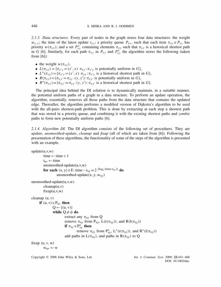
2.1.4. Algorithm DI. The DI algorithm consists of the following set of procedures. They areupdate, unsmoothed-update, cleanup and fixup (all of which are taken from [6]). Following thepresentation of these algorithms, the functionality of some of the steps of the algorithm is presentedwith an example.

update(u,v,w)time← time+1tuv← timeunsmoothed-update(u,v,w)for each (x,y)∈E : time− txy=2 [log2 (time-txy)] do

unsmoothed-update(x,y,wxy)

unsmoothed-update(u,v,w)cleanup(u,v)fixup(u,v,w)

cleanup (u,v)if (u,v)∈Puv then

Q←{(u,v)}while Q �=� do

extract any �xy from Qremove �xy from Pxy, L(r(�xy)), and R(l(�xy))if �xy∈P∗xy then

remove �xy from P∗xy, L∗(r(�xy)), and R∗(l(�xy))add paths in L(�xy), and paths in R(�xy) to Q

fixup (u,v,w)

wuv←w



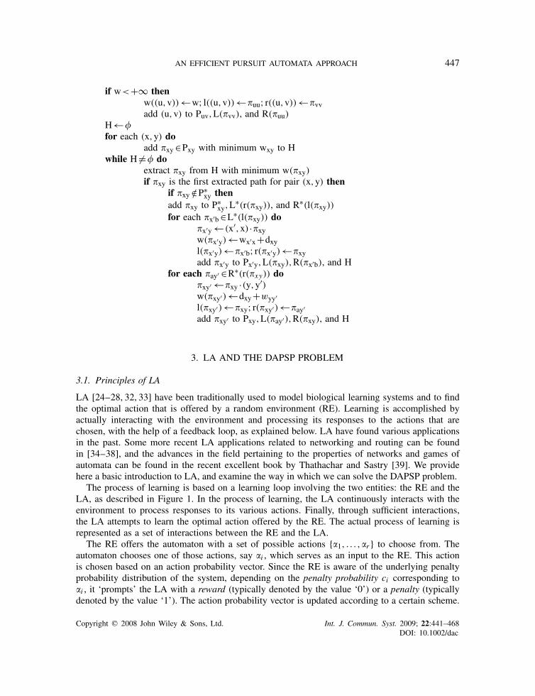
if w<+∞ thenw((u,v))←w; l((u,v))←�uu; r((u,v))←�vvadd (u,v) to Puv,L(�vv), and R(�uu)

H←�for each (x,y) do

add �xy∈Pxy with minimum wxy to Hwhile H �=� do

extract �xy from H with minimum w(�xy)if �xy is the first extracted path for pair (x,y) then

if �xy /∈P∗xy thenadd �xy to P∗xy,L∗(r(�xy)), and R∗(l(�xy))for each �x′b∈L∗(l(�xy)) do

�x′y←(x′,x) ·�xyw(�x′y)←wx′x+dxyl(�x′y)←�x′b; r(�x′y)←�xyadd �x′y to Px′y,L(�xy),R(�x′b), and H

for each �ay′ ∈R∗(r(�xy)) do�xy′ ←�xy ·(y,y′)w(�xy′)←dxy+wyy′l(�xy′)←�xy; r(�xy′)←�ay′add �xy′ to Pxy,L(�ay′),R(�xy), and H

3. LA AND THE DAPSP PROBLEM

3.1. Principles of LA

LA [24–28, 32, 33] have been traditionally used to model biological learning systems and to findthe optimal action that is offered by a random environment (RE). Learning is accomplished byactually interacting with the environment and processing its responses to the actions that arechosen, with the help of a feedback loop, as explained below. LA have found various applicationsin the past. Some more recent LA applications related to networking and routing can be foundin [34–38], and the advances in the field pertaining to the properties of networks and games ofautomata can be found in the recent excellent book by Thathachar and Sastry [39]. We providehere a basic introduction to LA, and examine the way in which we can solve the DAPSP problem.

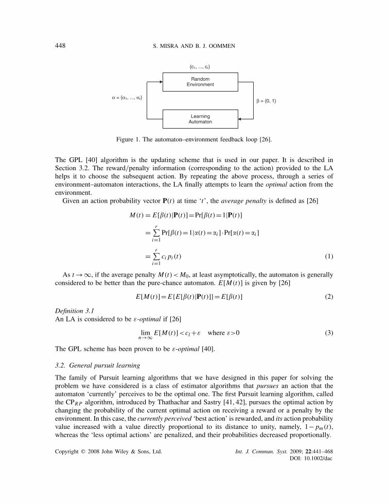
The process of learning is based on a learning loop involving the two entities: the RE and theLA, as described in Figure 1. In the process of learning, the LA continuously interacts with theenvironment to process responses to its various actions. Finally, through sufficient interactions,the LA attempts to learn the optimal action offered by the RE. The actual process of learning isrepresented as a set of interactions between the RE and the LA.

The RE offers the automaton with a set of possible actions {�1, . . . ,�r } to choose from. Theautomaton chooses one of those actions, say �i , which serves as an input to the RE. This actionis chosen based on an action probability vector. Since the RE is aware of the underlying penaltyprobability distribution of the system, depending on the penalty probability ci corresponding to�i , it ‘prompts’ the LA with a reward (typically denoted by the value ‘0’) or a penalty (typicallydenoted by the value ‘1’). The action probability vector is updated according to a certain scheme.



α = {α1, ..., αr}

RandomEnvironment

LearningAutomaton

{c1, ..., cr}

β = {0, 1}

Figure 1. The automaton–environment feedback loop [26].

The GPL [40] algorithm is the updating scheme that is used in our paper. It is described inSection 3.2. The reward/penalty information (corresponding to the action) provided to the LAhelps it to choose the subsequent action. By repeating the above process, through a series ofenvironment–automaton interactions, the LA finally attempts to learn the optimal action from theenvironment.

Given an action probability vector P(t) at time ‘t’, the average penalty is defined as [26]M(t)= E[�(t)|P(t)]=Pr[�(t)=1|P(t)]

=r∑

i=1Pr[�(t)=1|�(t)=�i ]·Pr[�(t)=�i ]

=r∑

i=1ci pi (t) (1)

As t→∞, if the average penalty M(t)<M0, at least asymptotically, the automaton is generallyconsidered to be better than the pure-chance automaton. E[M(t)] is given by [26]

E[M(t)]=E{E[�(t)|P(t)]}=E[�(t)] (2)

Definition 3.1An LA is considered to be ε-optimal if [26]

limn→∞E[M(t)]<cl+ε where ε>0 (3)

The GPL scheme has been proven to be ε-optimal [40].

3.2. General pursuit learning

The family of Pursuit learning algorithms that we have designed in this paper for solving theproblem we have considered is a class of estimator algorithms that pursues an action that theautomaton ‘currently’ perceives to be the optimal one. The first Pursuit learning algorithm, calledthe CPRP algorithm, introduced by Thathachar and Sastry [41, 42], pursues the optimal action bychanging the probability of the current optimal action on receiving a reward or a penalty by theenvironment. In this case, the currently perceived ‘best action’ is rewarded, and its action probabilityvalue increased with a value directly proportional to its distance to unity, namely, 1− pm(t),whereas the ‘less optimal actions’ are penalized, and their probabilities decreased proportionally.



To start with, based on the probability distribution P(t), the algorithm chooses an action �(t).Whether the response was a reward or a penalty, it increases that component of P(t) that hasthe maximal current reward estimate, and it decreases the probability corresponding to the restof the actions. Finally, the algorithm updates the running estimates of the reward probability ofthe actions chosen, this being the principal idea behind keeping and using the running estimates[41]. The estimate vector D̂(t) can be computed using the following formula, which yields themaximum likelihood estimate:

d̂i (t)= Wi (t)

Zi (t), ∀i=1,2, . . . ,r (4)

where Wi (t) is the number of times the action �i has been rewarded until the current time t andZi (t) is the number of times �i has been chosen until the current time t . Based on the aboveconcepts, the CPRP algorithm is formally given below without any further explanation.

Agache and Oommen [40] proposed a generalized version of the Pursuit algorithm (CPRP)

proposed by Thathachar and Sastry [41, 42]. Their algorithm, called the Generalized PursuitAlgorithm (GPA), generalizes Thathachar and Sastry’s Pursuit algorithm by pursuing all thoseactions that possess higher reward estimates than the chosen action. In this way, the probabilityof choosing a wrong action is minimized. Agache and Oommen experimentally compared theirPursuit algorithm with the existing algorithm, and found that their algorithm is the best in termsof the rate of convergence [40].

In the CPRP algorithm, the probability of the best-estimated action is maximized by firstdecreasing the probability of all the actions in the following manner:

p j (t+1)=(1−�)p j (t), j=1, . . . ,r (5)

The sum of the action probabilities is made unity, by the help of the probability mass �, whichis given by [40]

�=1−r∑

j=1p j (t+1)=1−

r∑

j=1(1−�)p j (t)=1−

r∑

j=1p j (t)+�

r∑

j=1p j (t)=� (6)

Thereafter, the probability mass � is added to the probability of the best-estimated action. TheGPA algorithm, thus, equi-distributes the probability mass � to the action estimated to be superiorto the chosen action. This gives us

pm(t+1)=(1−�)pm(t)+�=(1−�)pm(t)+� (7)

where d̂m=max j=1,...,r (d̂ j (t)).Thus, the updating scheme is given by

p j (t+1) = (1−�)p j (t)+ �

K (t)if d̂ j (t)>d̂i (t)

p j (t+1) = (1−�)p j (t) if d̂ j (t)� d̂i (t)

pi (t+1) = 1− ∑

j �=mp j (t)

(8)



where K (t) denotes the number of actions that have estimates greater than the estimate of theprobability reward of the action chosen at the given time instant.

3.3. Motivation behind APGP

As mentioned earlier, there is currently no efficient fast-converging solutions to the DAPSP problemfor use in graph scenarios when the edge-weights are dynamically and stochastically changing.We believe that the reason for this is that the existing models for this problem are inadequate forthis setting. We shall attempt to extend the current models by encapsulating the problem withinthe setting of the field of LA. To achieve this, we have to adequately model the three principalcomponents of any LA system, namely, the automaton, the environment and the reward–penaltystructure. In this context, we mention that in our case, the ‘system’ would imply a team of LAinteracting with the stochastic graph and playing a cooperative game. We shall now clarify howwe have achieved this.

The automata: We propose to station an LA at every node in the graph so as to invoke a game ofautomata operating in a sequential fashion. At every instance, its task is to choose a suitable edgefrom all the outgoing edges in that node to all the rest of the nodes in the graph. The intention, ofcourse, is that it guesses that this edge belongs to the shortest path between any pair of nodes fromthat node in the ‘average’ overall graph. It accomplishes this by interacting with the environment(described below). It first chooses an action from its prescribed set of actions. It then requests theenvironment for the current random edge-weight for the edge it has chosen. The system computesthe current shortest path by invoking the DI algorithm, where the LA determines whether thechoice it made should be rewarded or penalized as described below.

The environment: The environment consists of the overall dynamically changing graph. In thegraph, there are multiple edge-weights that change continuously and stochastically. These changesare based on a distribution that is unknown to the LA, but assumed to be known to the environment.In a religious LA–environment feedback, the environment also supplies a reward/penalty signal tothe LA. In our model, this feedback is inferred by the system, after it has invoked the DI algorithm.

Reward/Penalty: Based on the action that the LA has chosen (namely, an outgoing edge froma node, which the LA stochastically ‘guesses’ to belong to the shortest path between the pairof nodes), and the edge-weight that the environment provides, the updated shortest paths arecomputed. The effect of this choice is now determined by comparing the weight with the currentshortest paths for the ‘average’ graph, and the LA thus infers whether the choice should berewarded or penalized. The automaton then updates the action probabilities using the LRI scheme.In this present paper, we have opted to use the LRI scheme, but we are currently considering howestimator-based schemes can be used to lead to faster and superior solutions.

3.4. The GPL approach for solving DAPSP

Let G(V,E) denote a dynamically changing directed graph with a set of V nodes and E edges,which is to be processed by our algorithm. Suppose that we have such a dynamically changinggraph, where randomly selected edge-weights change depending on a probabilistic distribution.Our aim is to determine the underlying all-pairs shortest paths of the average weights, which thesystem is unaware of. Multiple edge-weight changes occur in the graph continuously at once. Let(u,v) denote an ordered pair of nodes representing a directed edge from u to v with a positivereal-valued weight, w(u,v). The algorithm computes the shortest paths between every possible



pair of nodes in the average graph, i.e. from every node s to every other node v∈V . The problemis to find an efficient algorithm for the above purpose.

3.4.1. Data structure for maintaining action probabilities. One way to approach the above-statedproblem could be to reuse the solution, named as GPSPA, which we proposed in our earlierpaper [43] on the dynamic single-source shortest-path problem. The way our previously proposedalgorithm [43] for the single-source shortest-path problem works is by maintaining an actionprobability vector corresponding to every automaton that is stationed at every node in the graph,and then using the collective responses between the team of interacting automata to maintain ashortest-path tree in the ‘average’ graph that will be stable regardless of the continuous randomlychanging weights. If we were to use such a strategy for solving the DAPSP problem, we would haveto determine a methodology by which we could maintain V shortest-path trees corresponding to theV nodes in the graph. However, such a solution would be obviously cumbersome and inefficient.

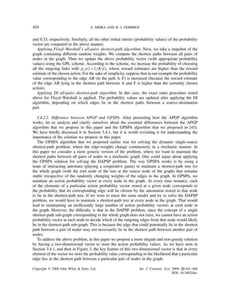
To address the above problem we propose to have a data structure for maintaining the actionprobabilities corresponding to all feasible pairs of nodes in the graph. The methodology used toimplement the data structure is unimportant to us, which can be a two-dimensional array, a linkedlist or any other suitable method. What is rather important is to visualize the data structure asa two-dimensional vector (matrix) (see Figure 3), whose columns represent all possible source–destination pairs in a particular graph, whereas the rows represent all possible outgoing edgesfrom each of the nodes in the graph. In such a representation the infeasible pairs of nodes orpairs between the same nodes are pre-processed and are omitted from further consideration inthe vector. At a particular time instant, each of the elements (entries) of the vector represents aprobability value corresponding to having an outgoing edge from a particular node (listed as rowsin the vector) in the source–destination pair (listed in the column). The usefulness of this datastructure will be further clarified in Section 3.4.2 using an example.

3.4.2. The APGP algorithm. The proposed solution to DAPSP, named as the APGP algorithm,is described here. Since insertions/deletions of edges are, respectively, equivalent to edge-weightdecreases/increases, this paper considers only the general case of weight decrease/increase oper-ations. The three efficiency considerations of the proposed algorithms investigated in this paperare: (a) the average number of nodes processed per operation, (b) the average number of edgesscanned per operation and (c) the average time per operation. These are discussed in further detailin Section 4.

The variant of the APGP algorithm that we consider in this paper is when APGP uses theDI algorithm [6], when an edge-weight increase/decrease occurs. Informally, the scheme is asfollows:

1. Obtain a snapshot of the given graph with each edge having a random cost. This cost isbased on the random call for an edge, where each cost has its own mean and variance. Thealgorithm maintains an action probability vector, P(t)={p1(t), p2(t), . . . , pr (t)}, for eachnode of the graph.

2. Run Floyd–Warshall’s all-pairs static algorithm once to determine the shortest-path edges onthe graph’s snapshot obtained in the first step.

3. (a) Update the action probability vector of each node according to the following scheme. Leti correspond to the outgoing link from a node, which is determined by Step 2 to belong tothe shortest-path link, and j correspond to all the other outgoing links from a node. Let K (t)



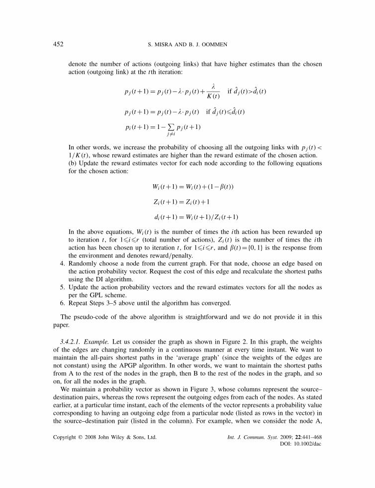
denote the number of actions (outgoing links) that have higher estimates than the chosenaction (outgoing link) at the t th iteration:

p j (t+1)= p j (t)−�· p j (t)+ �

K (t)if d̂ j (t)>d̂i (t)

p j (t+1)= p j (t)−�· p j (t) if d̂ j (t)�d̂i (t)

pi (t+1)= 1−∑

j �=ip j (t+1)

In other words, we increase the probability of choosing all the outgoing links with p j (t)<1/K (t), whose reward estimates are higher than the reward estimate of the chosen action.(b) Update the reward estimates vector for each node according to the following equationsfor the chosen action:

Wi (t+1)=Wi (t)+(1−�(t))

Zi (t+1)= Zi (t)+1di (t+1)=Wi (t+1)/Zi (t+1)

In the above equations, Wi (t) is the number of times the i th action has been rewarded upto iteration t , for 1�i�r (total number of actions), Zi (t) is the number of times the i thaction has been chosen up to iteration t , for 1�i�r , and �(t)={0,1} is the response fromthe environment and denotes reward/penalty.

4. Randomly choose a node from the current graph. For that node, choose an edge based onthe action probability vector. Request the cost of this edge and recalculate the shortest pathsusing the DI algorithm.

5. Update the action probability vectors and the reward estimates vectors for all the nodes asper the GPL scheme.

6. Repeat Steps 3–5 above until the algorithm has converged.

The pseudo-code of the above algorithm is straightforward and we do not provide it in thispaper.

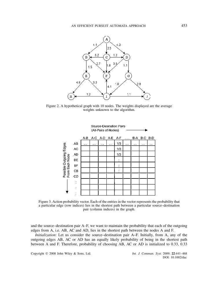
3.4.2.1. Example. Let us consider the graph as shown in Figure 2. In this graph, the weightsof the edges are changing randomly in a continuous manner at every time instant. We want tomaintain the all-pairs shortest paths in the ‘average graph’ (since the weights of the edges arenot constant) using the APGP algorithm. In other words, we want to maintain the shortest pathsfrom A to the rest of the nodes in the graph, then B to the rest of the nodes in the graph, and soon, for all the nodes in the graph.

We maintain a probability vector as shown in Figure 3, whose columns represent the source–destination pairs, whereas the rows represent the outgoing edges from each of the nodes. As statedearlier, at a particular time instant, each of the elements of the vector represents a probability valuecorresponding to having an outgoing edge from a particular node (listed as rows in the vector) inthe source–destination pair (listed in the column). For example, when we consider the node A,



Figure 2. A hypothetical graph with 10 nodes. The weights displayed are the averageweights unknown to the algorithm.

Figure 3. Action probability vector. Each of the entries in the vector represents the probability thata particular edge (row indices) lies in the shortest path between a particular source–destination

pair (column indices) in the graph.

and the source–destination pair A–F, we want to maintain the probability that each of the outgoingedges from A, i.e. AB, AC and AD, lies in the shortest path between the nodes A and F.

Initialization: Let us consider the source–destination pair A–F. Initially, from A, any of theoutgoing edges AB, AC or AD has an equally likely probability of being in the shortest pathbetween A and F. Therefore, probability of choosing AB, AC or AD is initialized to 0.33, 0.33



and 0.33, respectively. Similarly, all the other initial entries (probability values) of the probabilityvector are computed in the above manner.

Applying Floyd–Warshall’s all-pairs shortest-path algorithm: Next, we take a snapshot of thegraph containing different random weights. We compute the shortest paths between all pairs ofnodes in the graph. Then we update the above probability vector (with appropriate probabilityvalues) using the GPL scheme. According to the scheme, we increase the probability of choosingall the outgoing links with p j (t)<1/K (t), whose reward estimates are higher than the rewardestimate of the chosen action. For the sake of simplicity, suppose that in our example the probabilityvalue corresponding to the edge AB (in the path A–F) is increased (because the reward estimateof the edge AB lying in the shortest path between A and F is higher than the currently chosenaction).

Applying DI all-pairs shortest-path algorithm: In this case, the exact same procedure statedabove for Floyd–Warshall is applied. The probability values are updated after applying the DIalgorithm, depending on which edges lie in the shortest paths between a source–destinationpair.

3.4.2.2. Difference between APGP and GPSPA. After presenting how the APGP algorithmworks, let us analyze and clarify ourselves about the essential differences between the APGPalgorithm that we propose in this paper and the GPSPA algorithm that we proposed in [43].We have briefly discussed it in Section 3.4.1, but it is worth revisiting it for understanding theimportance of the solution we propose in this paper.

The GPSPA algorithm that we proposed earlier was for solving the dynamic single-sourceshortest-path problem, where the edge-weights change continuously in a stochastic manner. Inthis paper we consider a more generic version of the problem, where we want to maintain theshortest paths between all pairs of nodes in a stochastic graph. One could argue about applyingthe GPSPA solution for solving the DAPSP problem. The way GPSPA works is by using ateam of interacting automata (playing a cooperative game) to maintain a shortest-path tree forthe whole graph (with the root node of the tree at the source node of the graph) that remainsstable irrespective of the randomly changing weights of the edges in the graph. In GPSPA, wemaintain an action probability vector at every node in the graph. At every time instance, eachof the elements of a particular action probability vector stored at a given node corresponds tothe probability that its corresponding edge will be chosen by the automaton stored in that nodeto lie in the shortest-path tree. If we were to reuse the same model and try to solve the DAPSPproblem, we would have to maintain a shortest-path tree at every node in the graph. That wouldlead to maintaining an inefficiently large number of action probability vectors at each node inthe graph. However, the difficulty is that in the DAPSP problem, since the concept of a singleshortest-path sub-graph corresponding to the whole graph does not exist, we cannot have an actionprobability vector at each node to decide which of the outgoing edges from that node would likelybe in the shortest-path sub-graph. This is because the edge that could potentially lie in the shortestpath between a pair of nodes may not necessarily lie in the shortest path between another pair ofnodes.

To address the above problem, in this paper we propose a more elegant and non-greedy solutionby having a two-dimensional vector to store the action probability values. As we have seen inSection 3.4.1, and then in Figure 3, the key feature of this two-dimensional vector is that in everyelement of the vector we store the probability value corresponding to the likelihood that a particularedge lies in the shortest path between a particular pair of nodes in the graph.



3.4.2.3. Justification: why the algorithm works?. The formal reasoning of why the above algo-rithm works probably§§ relies on the ε-optimal property of the GPL scheme, the shortest-pathproperty of Floyd–Warshall’s algorithm and the update properties of DI. We provide below anintuitive reasoning (without a formal proof) in support of our above statement.

A close inspection of the APGP algorithm shows that the only place it calculates the shortest pathsis when executing Floyd–Warshall’s algorithm on the graph’s snapshot taken at the initializationstep and when executing the edge-weight update algorithm of DI. Floyd–Warshall’s algorithmis well known to find the optimal all-pairs shortest paths on a given graph topology. Since it isinitially executed on the static graph snapshot, it necessarily calculates the initial optimal all-pairsshortest paths. Furthermore, this means that, if the edge-weight update operates correctly, theupdated all-pairs shortest paths, obtained after invoking the DI scheme, will also be accurate. Byvirtue of the way the graph weights are presented to the algorithm, it is clear that as the numberof iterations tends to infinity, the computed average weight of the edges will converge towardtheir true mean values. Thus, the asymptotic shortest paths obtained over the different iterationsof APGP will converge toward the list of optimal all-pairs shortest paths obtained using the meanvalues. The proof that the all-pairs shortest paths are found with a probability as close to unity asdesired probably follows because of the fact that the action probability updating scheme, the GPL,is ε-optimal (this result would be certainly true if the choices of, and responses to, the individualautomata are independent); thus, the probability that a particular edge lies in the shortest pathbetween a particular source–destination pair in a graph will be arbitrarily close to unity. Therefore,as the number of iterations tends toward infinity, the probability of choosing the optimal actionfor each pairs of nodes tends toward unity, and the overall path costs will tend to the shortest-pathcosts of the mean edge-weights—which has also been confirmed experimentally.

With regard to the computational superiority, the DI algorithm continues to recalculate all theaffected shortest paths for every change in the edge-weights for the entire duration of executionof the algorithm. However, in such an environment, after convergence, the APGP algorithm willalready have attained to the list of optimal all-pairs shortest paths for the graph and, therefore,will do nothing in terms of re-computing the all-pairs shortest paths for every change in edge-weight. Therefore, after convergence, the performance of APGP in terms of the average number ofprocessed nodes, the average number of scanned edges and the average time per update operationwill be superior to the DI algorithm.

Although the proposed scheme is quite powerful, our algorithm, in its current form, has somelimitations as identified below. As it stands now, the algorithm has been designed for graphswhere the link structure is fixed. The number of actions of each automaton, which is equal to the‘valency’ of a node, is limited by the underlying graph structure (which is provided as an input tothe scheme in the initialization step). We believe that this limitation can possibly be rectified byallowing for a large actions set, equal to total number of nodes, at each node automaton, and thenapplying a data structure similar to the one proposed in Section 3.4.1. This increased set of actionsper node will have the effect of slowing down the convergence of the method and seems to be a

§§Unfortunately, theoretical analysis for this problem will be far from trivial. It turns out that the system that weencounter is a game of LA, because each automaton is not only responding to the environment (the randomlychanging graph), but also to the collective responses of the other automata. In this setting, not only do we haveno analysis, but we are also unaware of any available tools of analysis. Indeed, most of the currently availableanalyses for games of automata have to do with well-structured games, for example, two (or multi-person) zero-sumgames. The LA work for non-zero-sum games is sparse and a good reference can be found in [39]. But none ofthe models solved are applicable to our current problem domain.



bottleneck. We are currently studying this aspect of the algorithm and hope to resolve this in the nearfuture.

A final note on the rate of convergence of APGP is also not irrelevant. The rate of convergenceof stochastic systems is typically measured by the eigenvalues of the system, and by bounding thetime curve from above and below by sub-regular and super-regular functions [26]. This has beendone in the literature only for absolutely expedient schemes, but, as far as we know, no analysishas been done for such games of automata. We thus believe that the best that we (or the state ofthe art) can offer is the experimental demonstration of the rate of convergence and its comparisonwith the other existing schemes. This is what we currently embark on.

4. EXPERIMENTAL DETAILS

4.1. Experimental design

Several experiments, as stated below, are designed to evaluate the performance of APGP. However,in this paper we report a subset of the important results:

(1) Experiment Set 1: Comparison of the performance of APGP with that of DI for a graphwith a fixed number of nodes and sparsity of edges.

(2) Experiment Set 2: Comparison of the performance results with variation in the number ofnodes and sparsity of edges in the graph.

(3) Experiment Set 3: Sensitivity of the performance of APGP to the variation of certainparameters, while keeping other parameters constant.

For the above experiments, two random generators were built:

• Random graph topology generator: This module builds a random directed graph with n nodes,e edges and positive real edge-weights. The edge-weights are randomly generated and arenormally distributed. The random graph can be built from either specifying the number ofnodes and edges or by specifying the graph sparsity (described below).• Update sequence generator: This module is a random generator of edge-weight increase/

decrease update sequences. It creates a mixed sequence of increase/decrease operations onedges chosen at random in the graph. During the experiments, the sequence generator waspreset such that at any instance the occurrence of an increase or decrease operation is equallylikely.

The algorithms were tested both on manually entered and randomly generated graphs. However,the results shown in Section 4.3 were generated using random synthetic graphs only, as thatpermitted greater flexibility in changing the experimental parameters.

All the algorithms were tested with graphs of similar nature, i.e. graphs with directededges, positive real-valued edge-weights that are normally distributed and with stochastic edge-updates. Only the two edge operations, namely, edge-weight increase/decrease, were considered.This was because, as discussed earlier, edge-deletion/insertion is equivalent to edge-weightincrease/decrease, respectively. In addition, all discussions use the term sparsity of graphs,measured in percentage, to signify the number of edges in the graph as compared with the numberof nodes. The percentage density of the graphs can be obtained by subtracting the value of sparsityfrom 100.



4.2. Performance metrics

Three metrics were used for evaluating the performance of the algorithms invoked in the experi-ments:

• Number of scanned edges: This quantity measures the number of edges that are scanned inedge-weight increase/decrease operations. The first scanned edge is the edge whose weightis changed. Next, when an edge is scanned to check if it is in the shortest path between asource–destination pair, its value is incremented.• Number of processed nodes: This quantity measures the number of nodes that are processed in

edge-weight increase/decrease operations. It is incremented each time a node in the algorithmis removed from the priority queue that stores the nodes for processing.• Time required per update operation: This quantity is the running time required to update

weights and to obtain all the shortest paths.

Although our study considered only the above-mentioned three metrics, it is clear that othermetrics can also be proposed to assess the performance of our algorithms. A few of these possiblemetrics are:

(i) Average time taken for a single execution of the algorithm over several executions.(ii) Maximum time taken for a single execution of the algorithm over several executions.(iii) Minimum time taken for a single execution of the algorithm over several executions.(iv) Average amount of space consumed for a single execution of the algorithm over several

executions.(v) Maximum space consumed for a single execution of the algorithm over several executions.(vi) Minimum space consumed for a single execution of the algorithm over several executions.(vii) Time for initialization of the data structures of the algorithms.(viii) Average number of nodes processed in the distance update phase of the algorithms.(ix) Average number of edges scanned in the distance update phase of the algorithms.

While the above-mentioned measures (i)–(ix) can also be utilized to compare the performanceof the algorithms considered in the study, we suggest that they are not as important (as the oneswe have currently utilized) in judging the performance of any DAPSP algorithm. A responsiveDAPSP algorithm should be able to adapt itself to topology updates in the least possible time, byprocessing the least number of nodes, and by scanning the least number of edges for each updateoperation. From this perspective, the overall time computation measures (i)–(iii) are less importantthan the time taken per update operation. Furthermore, because of the decreasing costs of storagein the market, we believe that the space complexity measures (iv)–(vi) should not be considered tobe significant. Finally, although the performance measures (vii)–(ix) are valid for comparing thepreviously proposed dynamic algorithms, since APGP essentially invokes the DI algorithm, webelieve that these measures are not that significant in the current setting. However, we emphasizethat this is merely our perspective.

4.3. Experimental results

This section reports the results of the experiments that were conducted to examine the perfor-mance of APGP. The performance was compared with respect to the three indicators discussedin Section 4.2. Several experiments were performed on random graph topologies and random



edge-update sequences for different parameters. The experiments showed that APGP does notperform well at the beginning, i.e. when the algorithm is learning, but after the algorithm haslearned, APGP outperforms the DI algorithm. The results of the three sets of experiments aresummarized below. Only the running average values of the different metrics over the wholesequence of update operations are plotted in the graphs below. The programs keep track of theserunning average values and they are cumulative in their nature.

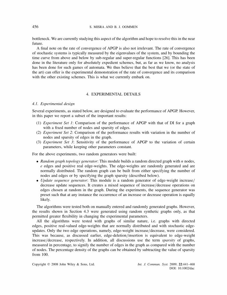
4.3.1. Experiment Set 1. The implementations of DI and APGP were run on mixed sequences of1000 modifying edge-update operations performed on a graph topology with 20 nodes and 50%sparsity. The edge-weights are random real values between 3.0 and 8.0. The value of the learningparameter, �, was set to 0.90.

The results of the experiment are shown in Figures 4–6. The results show 40–95% improvementof the performance of APGP with respect to that of DI. Inspection of the plots reveals that, initially,APGP performs worse than DI. This is quite expected, because initially APGP is unaware of thestochastic behavior of the environment, and is in the process of learning. But it does not takeit too long to converge. After this, APGP utilizes its knowledge about the environment, and itsperformance exceeds that of DI. After convergence, the average number of nodes processed, theaverage number of edges scanned and the average time spent per update operation are much lessfor APGP than for DI. For example, as seen from Figure 4, when the number of operations is 650,the average number of processed nodes for DI is approximately 28, whereas the average numberof processed nodes for APGP is approximately 2.

Experiments were run on other graph topologies as well and they yielded similar results. APGPwas consistently found to be superior with respect to these three metrics in all the experimentsconducted.

0

10

20

30

40

50

60

70

80

1 37 73 109

145

181

217

253

289

325

361

397

433

469

505

541

577

613

649

685

721

757

793

829

865

901

937

973

Operations

Ave

rag

e p

roce

ssed

no

des

APGPDI

Figure 4. Average processed nodes.



0

100

200

300

400

500

600

700

800

900

1 37 73 109

145

181

217

253

289

325

361

397

433

469

505

541

577

613

649

685

721

757

793

829

865

901

937

973

Operations

Ave

rag

e sc

ann

ed e

dg

es

APGP DI

Figure 5. Average scanned edges.

0

10

20

30

40

50

60

70

80

90

100

1 42 83 124

165

206

247

288

329

370

411

452

493

534

575

616

657

698

739

780

821

862

903

944

985

Operations

Ave

rag

e ti

me

req

uir

ed p

er u

pd

ate

APGPDI

Figure 6. Average time per update.

4.3.2. Experiment Set 2. A second set of experiments was conducted to evaluate the algorithmswith a variation of the graph structure, specifically, the graph sparsity, and the number of nodesin the graphs. In other words, our aim was to observe whether there was a different trend in



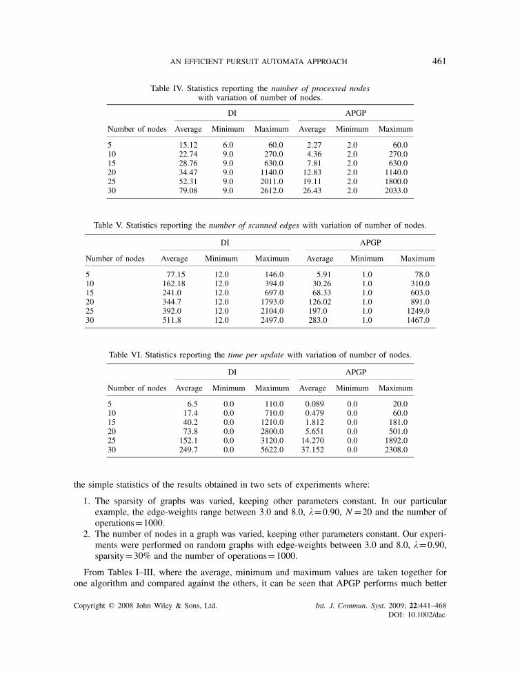
performance results when the structures of the graphs were varied, keeping other parametersconstant.

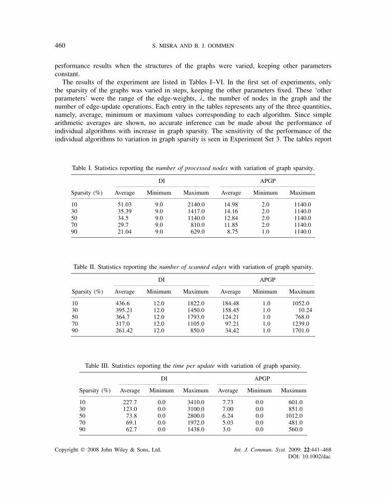
The results of the experiment are listed in Tables I–VI. In the first set of experiments, onlythe sparsity of the graphs was varied in steps, keeping the other parameters fixed. These ‘otherparameters’ were the range of the edge-weights, �, the number of nodes in the graph and thenumber of edge-update operations. Each entry in the tables represents any of the three quantities,namely, average, minimum or maximum values corresponding to each algorithm. Since simplearithmetic averages are shown, no accurate inference can be made about the performance ofindividual algorithms with increase in graph sparsity. The sensitivity of the performance of theindividual algorithms to variation in graph sparsity is seen in Experiment Set 3. The tables report

Table I. Statistics reporting the number of processed nodes with variation of graph sparsity.

DI APGP

Sparsity (%) Average Minimum Maximum Average Minimum Maximum

10 51.03 9.0 2140.0 14.98 2.0 1140.030 35.39 9.0 1417.0 14.16 2.0 1140.050 34.5 9.0 1140.0 12.84 2.0 1140.070 29.7 9.0 810.0 11.85 2.0 1140.090 21.04 9.0 629.0 8.75 1.0 1140.0

Table II. Statistics reporting the number of scanned edges with variation of graph sparsity.

DI APGP


10 436.6 12.0 1822.0 184.48 1.0 1052.030 395.21 12.0 1450.0 158.45 1.0 10.2450 364.7 12.0 1793.0 124.21 1.0 768.070 317.0 12.0 1105.0 97.21 1.0 1239.090 261.42 12.0 850.0 34.42 1.0 1701.0

Table III. Statistics reporting the time per update with variation of graph sparsity.

DI APGP


10 227.7 0.0 3410.0 7.73 0.0 601.030 123.0 0.0 3100.0 7.00 0.0 851.050 73.8 0.0 2800.0 6.24 0.0 1012.070 69.1 0.0 1972.0 5.03 0.0 481.090 62.7 0.0 1438.0 3.0 0.0 560.0



Table IV. Statistics reporting the number of processed nodeswith variation of number of nodes.

DI APGP

Number of nodes Average Minimum Maximum Average Minimum Maximum

5 15.12 6.0 60.0 2.27 2.0 60.010 22.74 9.0 270.0 4.36 2.0 270.015 28.76 9.0 630.0 7.81 2.0 630.020 34.47 9.0 1140.0 12.83 2.0 1140.025 52.31 9.0 2011.0 19.11 2.0 1800.030 79.08 9.0 2612.0 26.43 2.0 2033.0

Table V. Statistics reporting the number of scanned edges with variation of number of nodes.

DI APGP


5 77.15 12.0 146.0 5.91 1.0 78.010 162.18 12.0 394.0 30.26 1.0 310.015 241.0 12.0 697.0 68.33 1.0 603.020 344.7 12.0 1793.0 126.02 1.0 891.025 392.0 12.0 2104.0 197.0 1.0 1249.030 511.8 12.0 2497.0 283.0 1.0 1467.0

Table VI. Statistics reporting the time per update with variation of number of nodes.

DI APGP


5 6.5 0.0 110.0 0.089 0.0 20.010 17.4 0.0 710.0 0.479 0.0 60.015 40.2 0.0 1210.0 1.812 0.0 181.020 73.8 0.0 2800.0 5.651 0.0 501.025 152.1 0.0 3120.0 14.270 0.0 1892.030 249.7 0.0 5622.0 37.152 0.0 2308.0

the simple statistics of the results obtained in two sets of experiments where:

1. The sparsity of graphs was varied, keeping other parameters constant. In our particularexample, the edge-weights range between 3.0 and 8.0, �=0.90, N=20 and the number ofoperations=1000.

2. The number of nodes in a graph was varied, keeping other parameters constant. Our experi-ments were performed on random graphs with edge-weights between 3.0 and 8.0, �=0.90,sparsity=30% and the number of operations=1000.

From Tables I–III, where the average, minimum and maximum values are taken together forone algorithm and compared against the others, it can be seen that APGP performs much better



0

5

10

15

20

25

30

35

1 38 75 112

149

186

223

260

297

334

371

408

445

482

519

556

593

630

667

704

741

778

815

852

889

926

963

Operations

Ave

rag

e p

roce

ssed

no

des

0.90

0.930.96 0.98

0.87

Figure 7. Sensitivity of average processed nodes in APGP with the variation in learning parameter.

than the DI algorithm across different graph structures with varying graph sparsities. For example,from Table I, we see that the average value of time per update for APGP at 10% sparsity is 14.98,whereas that of DI is 51.03. This shows that on an average APGP processes less number of nodesper update operation than the DI algorithm. Similar results can be observed in the Tables IV–VI,when the number of nodes in the graph is varied.

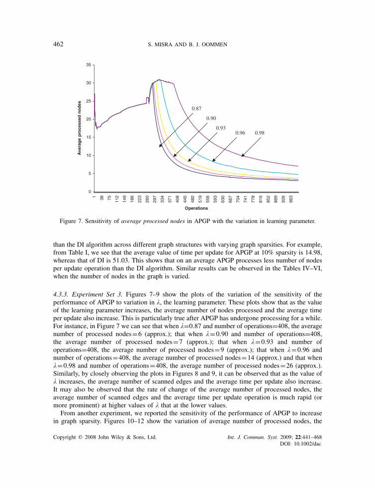
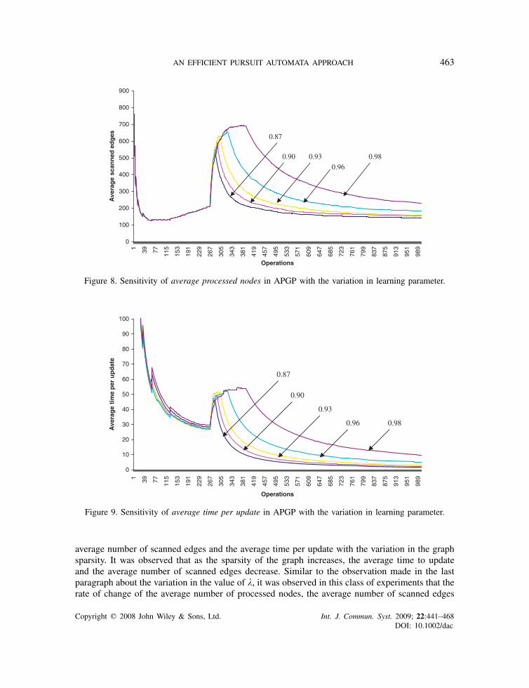
4.3.3. Experiment Set 3. Figures 7–9 show the plots of the variation of the sensitivity of theperformance of APGP to variation in �, the learning parameter. These plots show that as the valueof the learning parameter increases, the average number of nodes processed and the average timeper update also increase. This is particularly true after APGP has undergone processing for a while.For instance, in Figure 7 we can see that when �=0.87 and number of operations=408, the averagenumber of processed nodes=6 (approx.); that when �=0.90 and number of operations=408,the average number of processed nodes=7 (approx.); that when �=0.93 and number ofoperations=408, the average number of processed nodes=9 (approx.); that when �=0.96 andnumber of operations=408, the average number of processed nodes=14 (approx.) and that when�=0.98 and number of operations=408, the average number of processed nodes=26 (approx.).Similarly, by closely observing the plots in Figures 8 and 9, it can be observed that as the value of� increases, the average number of scanned edges and the average time per update also increase.It may also be observed that the rate of change of the average number of processed nodes, theaverage number of scanned edges and the average time per update operation is much rapid (ormore prominent) at higher values of � that at the lower values.

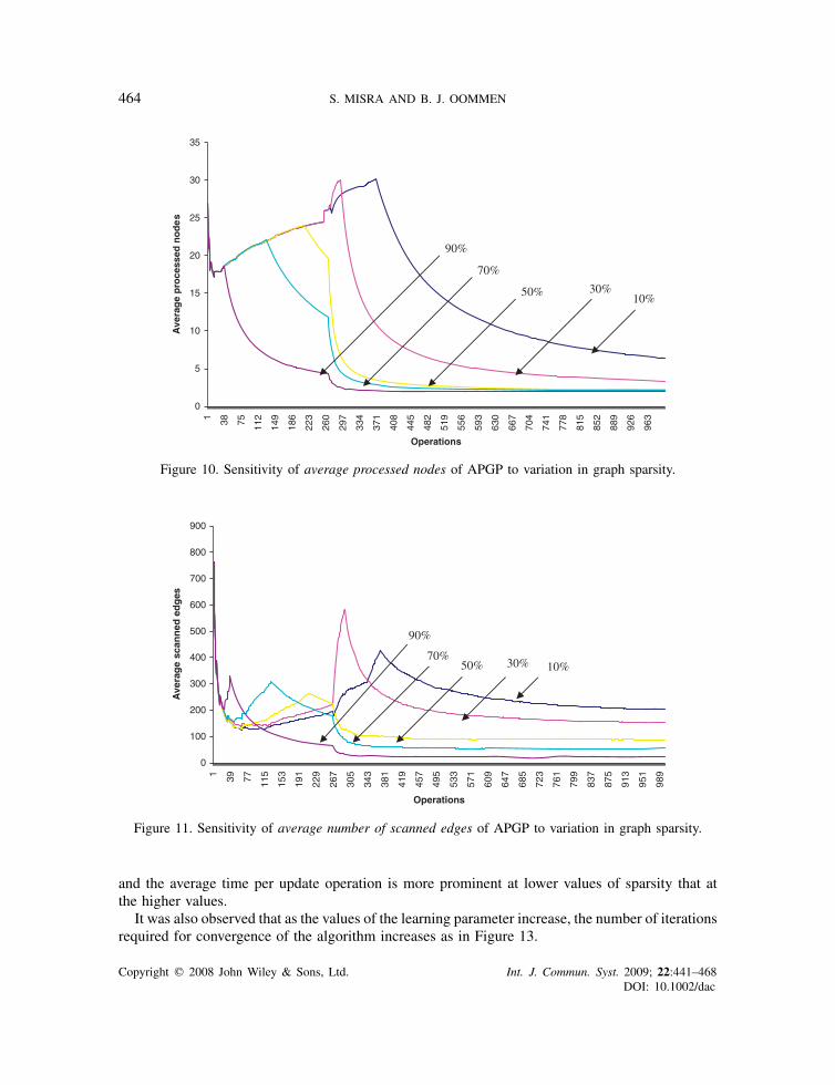
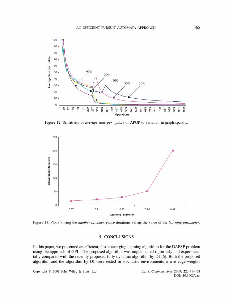
From another experiment, we reported the sensitivity of the performance of APGP to increasein graph sparsity. Figures 10–12 show the variation of average number of processed nodes, the



0

100

200

300

400

500

600

700

800

900

1 39 77 115

153

191

229

267

305

343

381

419

457

495

533

571

609

647

685

723

761

799

837

875

913

951

989

Operations

Ave

rag

e s

can

ned

ed

ges 0.87

0.90 0.93

0.96

0.98

Figure 8. Sensitivity of average processed nodes in APGP with the variation in learning parameter.

0

10

20

30

40

50

60

70

80

90

100

1 39 77 115

153

191

229

267

305

343

381

419

457

495

533

571

609

647

685

723

761

799

837

875

913

951

989

Operations

Ave

rag

e t

ime

per

up

dat

e

0.87

0.90

0.93

0.96 0.98

Figure 9. Sensitivity of average time per update in APGP with the variation in learning parameter.

average number of scanned edges and the average time per update with the variation in the graphsparsity. It was observed that as the sparsity of the graph increases, the average time to updateand the average number of scanned edges decrease. Similar to the observation made in the lastparagraph about the variation in the value of �, it was observed in this class of experiments that therate of change of the average number of processed nodes, the average number of scanned edges



0

5

10

15

20

25

30

35

1 38 75 112

149

186

223

260

297

334

371

408

445

482

519

556

593

630

667

704

741

778

815

852

889

926

963

Operations

Ave

rag

e p

roce

ssed

no

de

s

10%30%50%

70%

90%

Figure 10. Sensitivity of average processed nodes of APGP to variation in graph sparsity.

0

100

200

300

400

500

600

700

800

900

1 39 77 115

153

191

229

267

305

343

381

419

457

495

533

571

609

647

685

723

761

799

837

875

913

951

989

Operations

Ave

rag

e s

can

ned

ed

ges

90%

50%70%

30% 10%

Figure 11. Sensitivity of average number of scanned edges of APGP to variation in graph sparsity.

and the average time per update operation is more prominent at lower values of sparsity that atthe higher values.

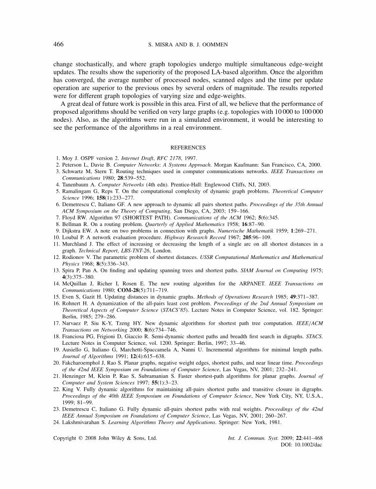
It was also observed that as the values of the learning parameter increase, the number of iterationsrequired for convergence of the algorithm increases as in Figure 13.



0

10

20

30

40

50

60

70

80

90

100

1 39 77 115

153

191

229

267

305

343

381

419

457

495

533

571

609

647

685

723

761

799

837

875

913

951

989

Operations

Ave

rag

e ti

me

per

up

dat

e

10%30%50%

70%90%

Figure 12. Sensitivity of average time per update of APGP to variation in graph sparsity.

0

50

100

150

200

250

0.87 0.9 0.93 0.96 0.99

Learning Parameter

Co

nver

gen

ce it

erat

ion

s

Figure 13. Plot showing the number of convergence iterations versus the value of the learning parameter.

5. CONCLUSIONS

In this paper, we presented an efficient, fast-converging learning algorithm for the DAPSP problemusing the approach of GPL. The proposed algorithm was implemented rigorously and experimen-tally compared with the recently proposed fully dynamic algorithm by DI [6]. Both the proposedalgorithm and the algorithm by DI were tested in stochastic environments where edge-weights



change stochastically, and where graph topologies undergo multiple simultaneous edge-weightupdates. The results show the superiority of the proposed LA-based algorithm. Once the algorithmhas converged, the average number of processed nodes, scanned edges and the time per updateoperation are superior to the previous ones by several orders of magnitude. The results reportedwere for different graph topologies of varying size and edge-weights.

A great deal of future work is possible in this area. First of all, we believe that the performance ofproposed algorithms should be verified on very large graphs (e.g. topologies with 10 000 to 100 000nodes). Also, as the algorithms were run in a simulated environment, it would be interesting tosee the performance of the algorithms in a real environment.

REFERENCES

1. Moy J. OSPF version 2. Internet Draft, RFC 2178, 1997.2. Peterson L, Davie B. Computer Networks: A Systems Approach. Morgan Kaufmann: San Francisco, CA, 2000.3. Schwartz M, Stern T. Routing techniques used in computer communications networks. IEEE Transactions on

Communications 1980; 28:539–552.4. Tanenbaum A. Computer Networks (4th edn). Prentice-Hall: Englewood Cliffs, NJ, 2003.5. Ramalingam G, Reps T. On the computational complexity of dynamic graph problems. Theoretical Computer

Science 1996; 158(1):233–277.6. Demetrescu C, Italiano GF. A new approach to dynamic all pairs shortest paths. Proceedings of the 35th Annual

ACM Symposium on the Theory of Computing, San Diego, CA, 2003; 159–166.7. Floyd RW. Algorithm 97 (SHORTEST PATH). Communications of the ACM 1962; 5(6):345.8. Bellman R. On a routing problem. Quarterly of Applied Mathematics 1958; 16:87–90.9. Dijkstra EW. A note on two problems in connection with graphs. Numerische Mathematik 1959; 1:269–271.10. Loubal P. A network evaluation procedure. Highway Research Record 1967; 205:96–109.11. Murchland J. The effect of increasing or decreasing the length of a single arc on all shortest distances in a

graph. Technical Report, LBS-TNT-26, London.12. Rodionov V. The parametric problem of shortest distances. USSR Computational Mathematics and Mathematical

Physics 1968; 8(5):336–343.13. Spira P, Pan A. On finding and updating spanning trees and shortest paths. SIAM Journal on Computing 1975;

4(3):375–380.14. McQuillan J, Richer I, Rosen E. The new routing algorithm for the ARPANET. IEEE Transactions on

Communications 1980; COM-28(5):711–719.15. Even S, Gazit H. Updating distances in dynamic graphs. Methods of Operations Research 1985; 49:371–387.16. Rohnert H. A dynamization of the all-pairs least cost problem. Proceedings of the 2nd Annual Symposium on

Theoretical Aspects of Computer Science (STACS’85). Lecture Notes in Computer Science, vol. 182. Springer:Berlin, 1985; 279–286.

17. Narvaez P, Siu K-Y, Tzeng HY. New dynamic algorithms for shortest path tree computation. IEEE/ACMTransactions on Networking 2000; 8(6):734–746.

18. Franciosa PG, Frigioni D, Giaccio R. Semi-dynamic shortest paths and breadth first search in digraphs. STACS.Lecture Notes in Computer Science, vol. 1200. Springer: Berlin, 1997; 33–46.

19. Ausiello G, Italiano G, Marchetti-Spaccamela A, Nanni U. Incremental algorithms for minimal length paths.Journal of Algorithms 1991; 12(4):615–638.

20. Fakcharoemphol J, Rao S. Planar graphs, negative weight edges, shortest paths, and near linear time. Proceedingsof the 42nd IEEE Symposium on Foundations of Computer Science, Las Vegas, NV, 2001; 232–241.

21. Henzinger M, Klein P, Rao S, Subramanian S. Faster shortest-path algorithms for planar graphs. Journal ofComputer and System Sciences 1997; 55(1):3–23.

22. King V. Fully dynamic algorithms for maintaining all-pairs shortest paths and transitive closure in digraphs.Proceedings of the 40th IEEE Symposium on Foundations of Computer Science, New York City, NY, U.S.A.,1999; 81–99.

23. Demetrescu C, Italiano G. Fully dynamic all-pairs shortest paths with real weights. Proceedings of the 42ndIEEE Annual Symposium on Foundations of Computer Science, Las Vegas, NV, 2001; 260–267.

24. Lakshmivarahan S. Learning Algorithms Theory and Applications. Springer: New York, 1981.



25. Meybodi MR, Beigy H. New learning automata based algorithms for adaptation of backpropagation algorithmparameters. International Journal of Neural Systems 2002; 12(1):45–67.

26. Narendra KS, Thathachar MAL. Learning Automata. Prentice-Hall: Englewood Cliffs, NJ, 1989.27. Obaidat MS, Papadimitriou GI, Pomportsis AS. Learning automata: theory, paradigms and applications. IEEE

Transactions on Systems, Man, and Cybernetics 2002; 32(6):706–709.28. Obaidat MS, Papadimitriou GI, Pomportsis AI. Efficient fast learning automata. Information Sciences 2003;

157(203):121–133.29. Seredynski F. Distributed scheduling using simple learning machines. European Journal of Operational Research

1998; 107:401–413.30. Thathachar ML, Sastry PS. Estimator algorithms for learning automata. Proceedings of the Platinum Jubilee

Conference on Systems and Signal Processing. Department of Electrical Engineering, Indian Institute of Science:Bangalore, India, 1986.

31. Najim K, Poznyak AS. Learning Automata: Theory and Applications. Pergamon Press: Oxford, 1994.32. Poznyak AS, Najim K. Learning Automata and Stochastic Optimization. Springer: Berlin, 1997.33. Papadimitriou GI, Pomportsis AS. Learning-automata-based TDMA protocols for broadcast communication

systems with bursty traffic. IEEE Communications Letters 2000; 4(3):107–109.34. Atlasis AF, Loukas NH, Vasilakos AV. The use of learning algorithms in ATM networks call admission control

problem: a methodology. Computer Networks 2000; 34(3):341–353.35. Atlasis AF, Vasilakos AV. The use of reinforcement learning algorithms in traffic control of high speed networks.

Advances in Computer Intelligence and Learning. Kluwer Academic Publishers: Dordrecht, 2002; 353–369.36. Kabudian J, Meybodi MR, Homayounpour MM. Applying continuous action reinforcement learning automata

(CARLA) to global raining of hidden Markov models. Proceedings of the International Conference on InformationTechnology: Coding and Computing (ITCC’04), Las Vegas, NV, vol. 2, April 2004.

37. Obaidat MS, Papadimitriou GI, Pomportsis AI, Laskaridis HS. Learning automata-based bus arbitration forshared-medium AM switches. IEEE Transactions on Systems, Man, and Cybernetics, Part B 2002; 32(6):815–820.

38. Vasilakos AV, Salouros MP, Alasssis AF, Pedrycz W. Optimizing QoS routing in hierarchical ATM networksusing computational intelligence techniques. IEEE Transactions on Systems, Man, and Cybernetics, Part C 2003;33(3):297–312.

39. Thathachar MAL, Sastry PS. Networks of Learning Automata. Kluwer Academic Publishers: Dordrecht, 2003.40. Agache M, Oommen BJ. Generalized pursuit learning schemes: new families of continuous and discretized

learning automata. IEEE Transactions on Systems, Man, and Cybernetics 2002; 32(6):738–749.41. Thathachar MAL, Sastry PS. Pursuit algorithm for learning automata. Unpublished paper that is available from

the authors.42. Thathachar MAL, Sastry PS. A new approach to designing reinforcement schemes for learning automata. Presented

at the IEEE International Conference on Cybernetics and Society, Bombay, India, January 1984.43. Misra S, Oommen BJ. GPSPA: a new adaptive algorithm for maintaining shortest path routing trees in stochastic

networks. International Journal of Communications Systems 2004; 17(10):963–984.

AUTHORS’ BIOGRAPHIES

Dr Sudip Misra is an Assistant Professor in the School of Information Technology atthe Indian Institute of Technology Kharagpur, India. Prior to this he held academicaffiliations in Cornell University (U.S.A.), Yale University (U.S.A.), Nortel Networks(Canada) and the Government of Ontario (Canada). He received his PhD degree inComputer Science from Carleton University, in Ottawa, Canada, and the masters andbachelors degrees respectively from the University of New Brunswick, Fredericton,Canada, and the Indian Institute of Technology, Kharagpur, India. Dr Misra has severalyears of experience working in the academia, government, and the private sectors inresearch, teaching, consulting, project management, architecture, software design, andproduct engineering roles.

His current research interests include algorithm design and engineering for telecom-munication networks, software engineering for telecommunication applications, and

computational intelligence and soft computing applications in telecommunications.



Dr Misra is the author/editor of over 80 scholarly research papers and books. He has won five research paperawards in different conferences. He was also the recipient of several academic awards and fellowships such asthe (Canadian) Governor General’s Academic Gold Medal at Carleton University, the University OutstandingGraduate Student Award in the Doctoral level at Carleton University, and the Canadian Government’s prestigiousNSERC Post Doctoral Fellowship. His biography was also selected for inclusion in the 2006–2007 edition ofMarquis Who’s Who in Science and Engineering, and the 25th Edition of the Marquis Who’s Who in theWorld, California, U.S.A.

Dr Misra is the Editor-in-Chief of two journals—the International Journal of Communication Networksand Distributed Systems (IJCNDS) and the International Journal of Information and Coding Theory (IJICoT),U.K. He is an Associate Editor of the Telecommunication Systems Journal (Springer SBM), Security andCommunication Networks Journal (Wiley), International Journal of Communication Systems (Wiley), andthe EURASIP Journal of Wireless Communications and Networking. He is also an Editor/Editorial BoardMember/Editorial Review Board Member of the IET Communications Journal, Computers and ElectricalEngineering Journal (Elsevier), International Journal of Internet Protocol Technology, the International Journalof Theoretical and Applied Computer Science, the International Journal of Ad Hoc and Ubiquitous Computing,Journal of Internet Technology, and the Applied Intelligence Journal (Springer). He was invited to chair severalinternational conference/workshop programs and sessions. He has been serving in the program committees ofover a dozen international conferences. Dr Misra was also invited to deliver keynote lectures in around a dozeninternational conferences in U.S.A., Canada, Europe, Asia, and Africa.

B. John Oommen received the BTech degree from the Indian Institute of Technology,Madras, India, in 1975, the ME degree from the Indian Institute of Science, Bangalore,India, in 1977, and the MS and PhD degrees from Purdue University, West Lafayettte,Indiana, in 1979 and 1982, respectively. He joined the School of Computer Science atCarleton University, Ottawa, in the academic year 1981–1982, where he currently holdsthe rank of a full professor. He is also on the editorial boards of the IEEE Transactions onSystems, Man, and Cybernetics and Pattern Recognition. His research interests includeautomata learning, adaptive data structures, statistical and syntactic pattern recognition,stochastic algorithms, and partitioning algorithms. He is the author of more than 265refereed journal and conference publications. He is a fellow of the IEEE and the IAPR.In July 2006, he was awarded the honorary rank of Chancellor’s Professor, which is alifetime award from Carleton University.


Documents

An efficient pursuit automata approach for estimating stable all-pairs shortest paths in stochastic network environments