An exact algorithm for the identical parallel machine scheduling problem

European Journal of Operational Research 152 (2004) 758–769

www.elsevier.com/locate/dsw

Production, Manufacturing and Logistics

An exact algorithm for the identical parallelmachine scheduling problem

Ethel Mokotoff *

Department of Economics, Universidad de Alcal�aa, Plaza Victoria 3, 28802 Alcal�aa de Henares, Spain

Received 7 May 1999; accepted 21 August 2002

Abstract

The NP-hard classical deterministic scheduling problem of minimizing the makespan on identical parallel machines

is considered. The polyhedral structure of the problem is analyzed, and strong valid inequalities are identified for fixed

values of the makespan. Thus, partial linear descriptions of the associated polytope are obtained and used to build an

exact algorithm. Linear programming relaxations are solved iteratively until the integer solution is reached. The al-

gorithm includes a preprocessing phase which reformulates the problem and simplifies it. Different constructive rules

have been tried out in the computation of upper bound values and the incidence of this choice is reported. Compu-

tational results show that the proposed algorithm yields, in a short computational time, optimal solutions in almost all

tested cases.

� 2002 Elsevier B.V. All rights reserved.

Keywords: Optimization; Polyhedral combinatorics; Scheduling

1. Introduction

In the classical deterministic identical parallel

machine problem, there are a number of inde-

pendent jobs to be processed on a range of iden-

tical machines. Each job has to be carried out on

one of the machines during a fixed processing time,without preemption. The problem of finding the

schedule that optimizes the makespan is consid-

ered.

Where can this model be applied to real-life

situations? There are many examples in industry,

* Tel.: +34-91-885-4202; fax: +34-91-885-4239.

E-mail address: [email protected] (E. Mokotoff).

0377-2217/$ - see front matter � 2002 Elsevier B.V. All rights reserv

doi:10.1016/S0377-2217(02)00726-9

social sciences and computer science, where the

problem of job-allocation and total completion

time fit in with this model: production lines, pa-

tients in hospitals, share-time systems, to give but

three examples. In fact, any situation that deals

with a series of processing units and has a set of

jobs to be carried out on them are real-life exam-ples of this mathematical model.

This problem is known to be NP-complete since

PARTITION polynomially reduces to the special

case with two machines [5]. So over the years there

has been a great deal of research to develop ap-

proximation algorithms which can be applied. The

only way to secure optimal solutions is by enu-

merative techniques. Dynamic programming andbranch and bound (B&B) techniques have been

ed.

mail to: [email protected]

E. Mokotoff / European Journal of Operational Research 152 (2004) 758–769 759

used to find optimal solutions. (For a survey of

parallel machine scheduling problems, see [7]).

Here we are presenting an exact cutting plane

algorithm built from the identification of valid

inequalities for fixed values of the maximum

completion time. These valid inequalities havebeen successfully applied to develop an approxi-

mate algorithm [8] and corresponding ones have

been applied to develop an exact and an approxi-

mate algorithm for the unrelated parallel machine

case [9]. The algorithm is a cutting plane method,

which includes a specially-developed preprocessing

phase. From the analysis of applying different

constructive rules we have refined the value of theupper bound. Computational results show that, in

almost all tested cases, the problem can be solved

exactly, and confirm the intuitive idea of it being

much more efficient than the corresponding algo-

rithm when it is applied to the unrelated parallel

machines.

After briefly introducing the notation, assump-

tions and formulation, we present the algorithmwith examples and the results obtained in our

computational experiment. We conclude the paper

with a summary discussion on the obtained results

and further research directions.

1.1. Notation, assumptions and formulation

In the rest of the paper, we will use the fol-lowing notation:

Ji job i, i 2 N ¼ f1; . . . ; ngMj machine j, j 2 M ¼ f1; . . . ;mgpi processing time of job JiCi completion time of job JiCmax makespan, the maximum completion time

of all jobs Ji, Cmax ¼ maxfC1;C2; . . . ;Cngxij assignment variable

Consider a set J of n independent and non-

preemptive jobs, Ji; which must be carried out on a

set M of m machines, Mj; which have the same

speed, which we consider to be identical. There-

fore, each job is to be carried out on any one of the

machines and the processing times of each job, pi,are not affected by the machine processing it. In-

dependent jobs means that there is no precedence

among them, and non-preemption requires that

jobs must be completed once they have begun,

without interruption. The aim is to find an as-

signment of the n jobs to machines from set M that

minimizes the maximum completion time crite-

rion, called makespan.

The problem in hand is then denoted by P==Cmax,

where P represents identical parallel machines, the

jobs are not constrained, and the objective is to

produce the minimum length schedule.

A mixed integer programming (MIP) formula-

tion of the minimum makespan problem is as

follows:

min y

s:t:Xmj¼1

xij ¼ 1; 16 i6 n;ð1Þ

y �Xni¼1

pixij P 0; 16 j6m; ð2Þ

where the optimal value of y is Cmax and

xij ¼1 if job i is assigned to machine j0 if job i is not assigned to machine j

�

2. Cutting plane scheme

The proposed algorithm (PA) presents a cutting

plane scheme (see [4] for a survey of this field) built

from the identification of valid inequalities that

apply to the subset of the solutions constrained by

a maximum value of the makespan. The main part

of this algorithm consists in generating constraintswith the valid inequalities identified for P==Cmax in

[8]. The separation procedure checks whether or

not a given point, the optimum solution of the last

linear programming (LP) relaxation solved, is an

integral vector. If so, the algorithm stops, other-

wise some new valid inequalities are added to

truncate the last LP polyhedron.

For an algorithm such as that being presentedthe computation of fitting initial tight lower and

upper bounds is critical. Because refined bounds

may reduced the number of iterations, and con-

sequently the computational time, remarkably. (In

Section 4 we report about the benefit of computing

760 E. Mokotoff / European Journal of Operational Research 152 (2004) 758–769

the upper bound by means of the algorithms based

on list scheduling [3]).

Since the number of binary variables and in-

equalities is rather large even for moderately sized

multiple machine scheduling problems, we have

implemented a special preprocessing procedure inorder to keep the problem in a manageable size, as

well as to tighten the lower bound value.

The solution set F for the stated problem is

defined by ðx; yÞ

x 2 f0; 1gn�m;

y 2 Rþ;Pmj¼1 xij ¼ 1 8i 2 f1; . . . ; ng;

y �Pn

i¼1 pixij P 0 8j 2 f1; . . . ;mg:

8>><>>:The polyhedron P that defines the linear relaxationof F is obtained by substituting x 2 f0; 1gn�m

by

x 2 Rn�mþ . Due to the fact that

minfy : ðx; yÞ 2 F g ¼ minfy : ðx; yÞ 2 P ;

Axþ Dy6 bg;

where Axþ Dy6 b are valid linear inequalities that

together with the initial inequalities of P define the

so-called linear description of F (see e.g. [11]), a

method for identifying a valid inequality, which is

not satisfied by the solution of the LP relaxation

(should one exist), is the core of cutting plane

techniques. Iteratively, valid inequalities are added

and LP relaxations are solved, until a feasible so-lution to the combinatorial optimization problem

is obtained. If, after a number of iterations without

finding an integral solution, there is no new cut,

the algorithm makes use of B&B to complete the

search, taking the last solved LP relaxation as

initial solution, which may be good enough to ef-

ficiently reduce the number of nodes to be ex-

plored in the B&B procedure.

1 This will occur when there are no added constraints.

Then, at any iteration, after having added hP 0 constraints of

type 3 (added constraints), the linear programming problem has

mþ nþ h constraints in addition to the non-negativity condi-

tions. Therefore, an optimal LP solution has mþ nþ h basic

variables, including the slack variables corresponding to the

constraints of type 2 and 3, which may take positive values

while the other non-basic variables take the value zero. If the

solution is not integral, more than n assigning variables take

positive values. Thus, at least one constraint of type 2 or 3 are

satisfied as equality.

2.1. Valid inequalities

For a value y0 of y, we denote by F ðy0Þ thesubset of ðx; y0Þ 2 F . Let I be a family of valid

inequalities for convðF ðy0ÞÞ and let P ðIÞ be the

current relaxation of convðF ðy0ÞÞ defined by the

inequalities of P and the inequalities of I. Let

ðx0; y0Þ be a point of P ðIÞ that does not belong

to F ðy0Þ. We have to find a valid inequality I

such that convðF ðy0ÞÞ � P ðI [ fIgÞ and ðx0; y0Þ 62P ðI [ fIgÞ. To manage it we have drawn inspi-

ration from the ideas developed in [12] for the

upper bound flow model.

For each machineMj, let Sj ¼ fi 2 N jx0ij > 0g bethe set of jobs assigned (at least in part) to machineMj. If the machine constraint corresponding to

Mj is satisfied at equality by ðx0; y0Þ, that con-

straint is said to be active. Let Dj ¼P

i2Sj pi � y0 bethe excess charge of machine Mj and let S0

j ¼fk 2 Sjjpk > Djg be the subset of the jobs in Sjwhose processing time on Mj is greater than Dj.

Notice that the excess charge of Mj is positive ifPi2Sj pi > y0.The following proposition shows that for every

machine Mj, corresponding to an active constraint,

with positive excess charge Dj, and such that

S0j 6¼ f/g, a valid inequality is generated.

For any x 2 R, we let xþ denote the value

maxf0; xg.

Proposition 1. Let ðx0; y0Þ be a point of P ðIÞ andassume that the machine constraint for Mj is activefor ðx0; y0Þ 1. Then the linear inequality:Xi2Sj

pixij 6 y0 �Xi2Sj

ðpi � DjÞþð1� xijÞ ð3Þ

is a valid inequality for convðF ðy0ÞÞ. Moreover ifthere is a job Jk 2 S0

j for which x0k < 1, then the in-equality is not satisfied by ðx0; y0Þ.

Proof1. Since there is a job k 2 Sj such that pk > Dj, and

0 < x0kj < 1,Xi2Sj

ðpi � DjÞþð1� x0ijÞ > 0:


Thus, ifP

i2Sj pix0ij ¼ y0, the LP solution ðx0; y0Þ

does not satisfy the inequality (3).

2. Let ðx�; y�Þ be a solution for which x� is binary

and y� ¼ y0.

Let Bj ¼ fi 2 Sj=x�ij ¼ 0g,Xi2Sj

pix�ij ¼X

i2SjnBj

pi ¼Xi2Sj

pi �Xi2Bj

pi

¼ y0 þ Dj �Xi2Bj

pi ¼ y0 �Xi2Bj

pi

� Dj

!:

SinceP

i2Sj pix�ij cannot be greater than y� ¼ y0, it

is necessary thatP

i2Bjpi � Dj P 0.

Thus,P

i2Sj pix�ij ¼ y0 �

Pi2Bj

pi � Dj

�þ6 y0 �P

i2Bjðpi � DjÞþ.

On the other hand, since 1� x�ij ¼ 1 if i 2 Bj,

and 1� x�ij ¼ 0 if i 2 Sj � Bj, we have

y0 �Xi2Bj

ðpi � DjÞþ ¼ y0 �Xi2Bj

ðpi � DjÞþð1� x�ijÞ

�X

i2Sj�Bj

ðpi � DjÞþð1� x�ijÞ

¼ y0 �Xi2Sj

ðpi � DjÞþð1� x�ijÞ:

Thus, we can concludeXi2Sj

pix�ij 6 y0 �Xi2Sj

ðpi � DjÞþð1� x�ijÞ: �

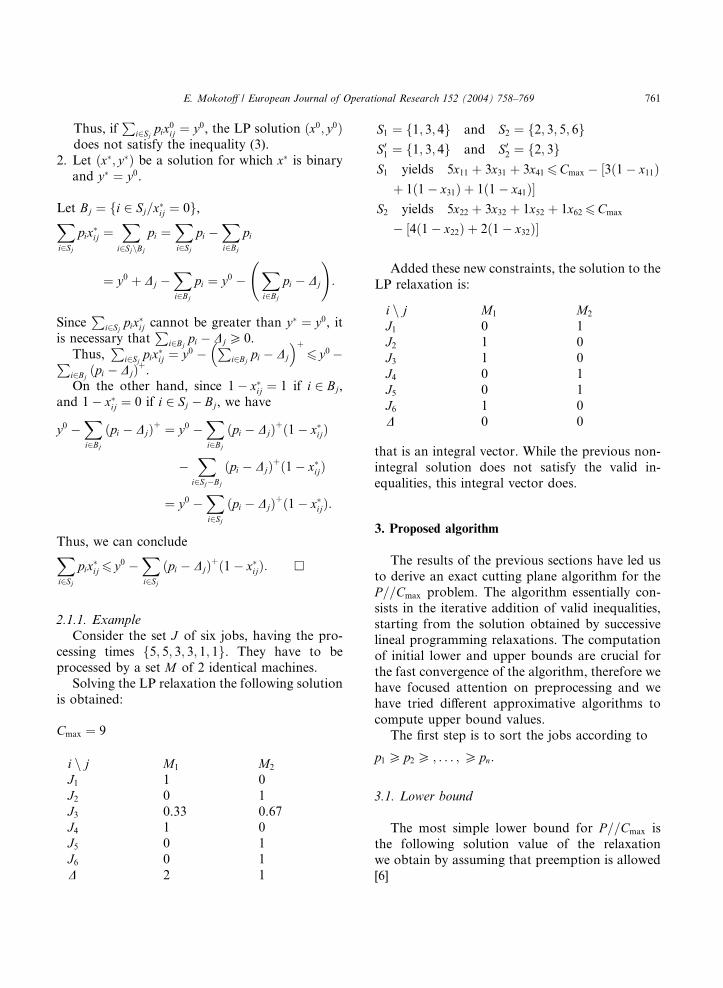
2.1.1. Example

Consider the set J of six jobs, having the pro-

cessing times f5; 5; 3; 3; 1; 1g. They have to be

processed by a set M of 2 identical machines.

Solving the LP relaxation the following solution

is obtained:

Cmax ¼ 9

i n j M1 M2

J1 1 0

J2 0 1

J3 0.33 0.67J4 1 0

J5 0 1

J6 0 1

D 2 1

S1 ¼ f1; 3; 4g and S2 ¼ f2; 3; 5; 6gS01 ¼ f1; 3; 4g and S0

2 ¼ f2; 3gS1 yields 5x11 þ 3x31 þ 3x41 6Cmax � ½3ð1� x11Þ

þ 1ð1� x31Þ þ 1ð1� x41Þ�S2 yields 5x22 þ 3x32 þ 1x52 þ 1x62 6Cmax

� ½4ð1� x22Þ þ 2ð1� x32Þ�

Added these new constraints, the solution to the

LP relaxation is:

that is an integral vector. While the previous non-

integral solution does not satisfy the valid in-

equalities, this integral vector does.

i n j M1 M2

J1 0 1

J2 1 0

J3 1 0

J4 0 1

J5 0 1

J6 1 0

D 0 0

3. Proposed algorithm

The results of the previous sections have led us

to derive an exact cutting plane algorithm for the

P==Cmax problem. The algorithm essentially con-

sists in the iterative addition of valid inequalities,

starting from the solution obtained by successivelineal programming relaxations. The computation

of initial lower and upper bounds are crucial for

the fast convergence of the algorithm, therefore we

have focused attention on preprocessing and we

have tried different approximative algorithms to

compute upper bound values.

The first step is to sort the jobs according to

p1 P p2 P ; . . . ; P pn:

3.1. Lower bound

The most simple lower bound for P==Cmax is

the following solution value of the relaxation

we obtain by assuming that preemption is allowed[6]


LBðCmaxÞ ¼ max1

m

Xni¼1

pi;maxi

fpig( )

:

This lower bound can be further improved by

considering that

Cmax P pm þ pmþ1:

Then, it is possible to tighten the bound as follows:

LBðCmaxÞ ¼ max1

m

Xni¼1

pi;maxi

fpig; pm

(þ pmþ1

):

Later, this bound can only be increased when the

linear program ensues unfeasible.

3.2. Upper bound

A feasible initial solution is built by means of

an approximative algorithm (AA). The obtained

value of Cmax is taken as the upper bound, i.e.,UBðCmaxÞ ¼ CmaxðAAÞ.

The classical longest processing time first (LPT)

heuristic [2] consists in making a list according to

LPT order and then, as with any list scheduling

algorithm, assigning the uppermost job from the

list to a free or to the least loaded machine, until

the list is exhausted. The MultiFit algorithm takes

into account the duality existing between theP==Cmax and the bin packing problem [1]. The

MultiFit algorithm performs better than the pre-

vious one by increasing the computational com-

plexity. We have also implemented other more

recent heuristics like those presented in [10] and [3]

based on list scheduling, some of which provide

similar results to MultiFit without pushing the

computational effort so much, and even taking lesstime than LPT in many cases.

3.3. Preprocessing

In the preprocessing phase, an essential part of

cutting plane algorithms, we try to reformulate the

problem to narrow the difference between the va-

lue of the objective function in the LP relaxation

and that of the MIP as much as possible. It con-

sists in the analysis of the given problem instance

in order to find a structure that helps to break

down the instance, to reduce its size, or to adjust

and tighten the MIP formulation. This can be

done by, for example, turning some inequalities

into equations, or fixing certain variables.

In the PA, by only using techniques specially

developed for the P==Cmax problem, we imple-

mented identification of infeasibilities and redun-dancies, improving bounds and coefficients, and

fixing variables. The preprocessing task presents

three stages that are described in the following.

3.3.1. Fixing variables

As the machines are identical, we can fix in

advance a job to any machine. By doing this, we

save m binary variables, and do not lose any fea-sible solution. Furthermore, we have eliminated

one constraint of type (1), and the right hand side

of the constraints of type (2) is subsequently im-

proved by this tightening adjustment.

3.3.2. Assigning variables

When we take into account the value of the

lower bound of Cmax, LBðCmaxÞ, we can identify

unfeasible and redundant solutions. We have to

check whether

pk þ pl 6LBðCmaxÞ

for a determined value of LBðCmaxÞ, to looking

into the possibility of two jobs with processing

times pk and pl being assigned to the same ma-

chine. Beginning with the first two jobs, p1 þ p2 iscompared with LBðCmaxÞ, if the sum is greater than

LBðCmaxÞ, the binary variable x21 is fixed at 0, andfollowing the same idea as that described in the

above paragraph, job J2 is assigned to machineM2,

and the x2j variables, for j ¼ 1; . . . ;m are fixed.

This procedure is applied to J2; J3; . . . ; Jm. The

corresponding constraints of type (1) are elimi-

nated, and the constraints of type (2) are also

improved by tightening their bounds.

3.3.3. Adding constraints

Having completed the first two stages, the ac-

tual LBðCmaxÞ for each machine is not necessary

the same. If job Ji was assigned to machine Mj as a

consequence of having applied previous stages,

then the lower bound LBðCmaxÞ for this machine

has decreased by pi. Thus, by analysis of each

machine�s new capacity value, it could be the case


that a machine cannot process a certain job, Jkwithout exceeding LBðCmaxÞ. If this is indeed the

case, we add the restriction

xkj ¼ 0:

The same analysis applies to the remaining jobsand machines.

3.4. Core of the algorithm

If the initial lower and upper bounds (obtained

by Section 3.1 and 3.2 respectively) coincide, the

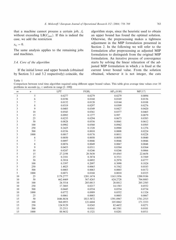
Table 1

Comparison between total time algorithm required using different up

problems in seconds (pij 2 uniform in range [1–100])

m n LPT FGH1

3 5 0.0277 0.0

3 6 0.0196 0.0

3 7 0.0152 0.0

3 8 0.0319 0.0

3 9 0.0405 0.0

3 10 0.0543 0.0

3 15 0.0992 0.1

3 25 0.0235 0.0

3 50 0.0828 0.0

3 100 0.0902 0.0

3 250 0.2425 0.1

3 500 0.0336 0.0

3 1000 0.0017 0.0

5 6 0.0050 0.0

5 7 0.0097 0.0

5 8 0.0076 0.0

5 9 0.0453 0.0

5 10 0.0247 0.0

5 15 27.2198 20.5

5 25 0.2181 0.3

5 50 0.3918 0.0

5 100 0.3397 0.2

5 250 1.4025 0.0

5 500 0.0003 0.0

5 1000 0.0071 0.0

10 25 1178.2777 1201.1

10 50 662.4469 567.4

10 100 24.5514 205.0

10 250 17.3885 0.0

10 500 0.0445 0.0

10 1000 0.0772 0.0

15 25 0.0061 0.0

15 50 1646.8634 1813.5

15 100 568.0953 121.6

15 250 124.9129 0.0

15 500 53.2511 0.0

15 1000 88.9632 0.1

algorithm stops, since the heuristic used to obtain

an upper bound has found the optimal solution.

Otherwise, the preprocessing makes a tightness

adjustment in the MIP formulation presented in

Section 2. In the following we will refer to the

formulation after preprocessing as adjusted MIPformulation to distinguish from the original MIP

formulation. An iterative process of convergence

starts by solving the linear relaxation of the ad-

justed MIP formulation in which y is fixed at the

current lower bound value. From the solution

obtained, whenever it is not integer, the cuts

per bound values. This table gives average time values over 10

AP10ð0:80Þ MFð17Þ279 0.0279 0.0094

160 0.0169 0.0156

120 0.0144 0.0108

297 0.0309 0.0276

349 0.0427 0.0420

361 0.0377 0.0465

277 0.997 0.0879

294 0.0673 0.0383

556 0.0841 0.0612

560 0.0942 0.0505

328 0.0988 0.1276

010 0.0008 0.0224

176 0.0011 0.0228

050 0.0050 0.0040

046 0.0046 0.0046

049 0.0067 0.0048

311 0.0384 0.0364

246 0.0246 0.0066

630 19.4565 22.6658

874 0.3511 0.3569

892 0.2970 0.0777

097 0.3090 0.1824

065 0.3362 0.0183

063 0.0003 0.0172

168 0.0010 0.0325

674 1163.1956 1200.9186

265 624.2728 704.8083

813 20.8812 205.2585

217 14.1583 0.0552

554 0.0554 0.0734

989 0.0552 0.1324

003 0.0003 0.0067

872 1391.8967 1761.2515

604 105.8862 171.3333

243 82.4432 0.0271

161 68.3381 0.0101

321 0.0281 0.0511


described in Section 2.1 are used to truncate the

polyhedron of the adjusted MIP formulation

where y is fixed. If the resultant linear relaxation

is not feasible, the lower bound is increased by

one unit. Unless the lower and upper bound

values coincide, the original MIP formulationis then retaken, with the updated lower bound

value, and the process, including the preprocessing

phase, restarts. The algorithm stops when a linear

relaxation gives an integral solution or lower and

upper bound values coincide. If no new cut is

found, we apply the B&B algorithm to the original

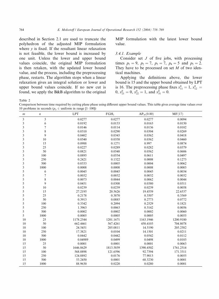
Table 2

Comparison between time required by cutting plane phase using differe

10 problems in seconds (pij 2 uniform in range [1–100])

m n LPT FGH1

3 5 0.0277 0.0

3 6 0.0192 0.0

3 7 0.0146 0.0

3 8 0.0310 0.0

3 9 0.0402 0.0

3 10 0.0540 0.0

3 15 0.0988 0.1

3 25 0.0227 0.0

3 50 0.0821 0.0

3 100 0.0895 0.0

3 250 0.2421 0.1

3 500 0.0333 0.0

3 1000 0.0008 0.0

5 6 0.0045 0.0

5 7 0.0032 0.0

5 8 0.0073 0.0

5 9 0.0451 0.0

5 10 0.0239 0.0

5 15 27.2195 20.5

5 25 0.2178 0.3

5 50 0.3913 0.0

5 100 0.3342 0.2

5 250 1.3963 0.0

5 500 0.0002 0.0

5 1000 0.0005 0.0

10 25 1178.2544 1201.1

10 50 662.4461 567.4

10 100 24.5451 205.0

10 250 17.3821 0.0

10 500 0.0442 0.0

10 1000 0.04989 0.0

15 25 0.0001 0.0

15 50 1646.8629 1813.5

15 100 568.0898 121.6

15 250 124.8892 0.0

15 500 53.2450 0.0

15 1000 88.9630 0.0

MIP formulation with the latest lower bound

value.

3.4.1. Example

Consider set J of five jobs, with processing

times p1 ¼ 9, p2 ¼ 7, p3 ¼ 7, p4 ¼ 5 and p5 ¼ 2.They have to be processed on set M of two iden-

tical machines.

Applying the definitions above, the lower

bound is 15 and the upper bound obtained by LPT

is 16. The preprocessing phase fixes x011 ¼ 1, x012 ¼0, x021 ¼ 0, x022 ¼ 1, and x031 ¼ 0.

nt upper bound values. This table gives average time values over

AP10ð0:80Þ MFð17Þ277 0.0277 0.0094

153 0.0163 0.0150

114 0.0136 0.0102

290 0.0304 0.0269

345 0.0362 0.0418

358 0.0362 0.0460

271 0.997 0.0874

289 0.0282 0.0379

548 0.0562 0.0606

554 0.0611 0.0497

322 0.0008 0.1273

005 0.0004 0.0062

008 0.0008 0.0003

045 0.0045 0.0034

032 0.0032 0.0032

044 0.0062 0.0044

308 0.0380 0.0311

239 0.0239 0.0058

626 19.4559 22.6537

870 0.3507 0.3569

885 0.2773 0.0772

094 0.2529 0.1821

063 0.3142 0.0056

002 0.0002 0.0060

005 0.0005 0.0055

671 1163.1946 1200.9180

261 450.4103 704.8078

811 14.5190 205.2582

104 14.1501 0.0211

442 0.0542 0.0112

499 0.0498 0.0103

001 0.0001 0.0063

859 1390.4502 1761.2514

596 92.7394 171.3311

176 77.9013 0.0055

001 68.3230 0.0001

220 0.0280 0.0001


Solving the first LP relaxation, which includes

the constraint y ¼ 15, the following solution is

obtained:

y0 ¼ 15

and

i n j M1 M2

1 1 0

2 0 1

3 0 1

4 0.8 0.2

5 1 0

D 1 4

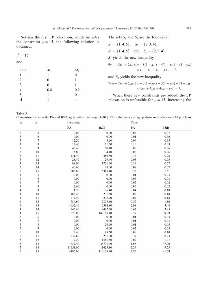
Table 3

Comparison between the PA and B&B, pij 2 uniform in range [1–100]

m n Iterations

PA B&B

3 5 0.00 0

3 6 0.00 0

3 7 12.20 3

3 8 17.40 21

3 9 48.40 50

3 10 15.80 34

3 11 131.40 460

3 12 28.40 29

3 13 98.00 1721

3 14 46.60 43

3 15 205.60 5318

4 5 0.00 0

4 6 0.00 0

4 7 0.00 0

4 8 2.60 0

4 9 1.20 196

4 10 185.40 231

4 11 277.40 275

4 12 784.60 2803

4 13 4052.40 6594

4 14 945.40 4492

4 15 520.80 109108

5 6 0.00 0

5 7 0.00 0

5 8 0.00 26

5 9 0.00 0

5 10 2.40 48

5 11 237.60 231

5 12 9.20 1581

5 13 1637.40 25771

5 14 11658.00 11653

5 15 4496.00 110108

The sets Sj and S0j are the following:

S1 ¼ f1; 4; 5g; S2 ¼ f2; 3; 4g;S01 ¼ f1; 4; 5g and S0

2 ¼ f2; 3; 4g:S1 yields the new inequality

9x11 þ 5x41 þ 2x516 y � 8ð1� x11Þ � 4ð1� x41Þ � ð1� x51Þ� x11 þ x41 þ x51 � y6 � 13

and S2 yields the new inequality

7x22 þ 7x32 þ 5x426 y � 3ð1� x22Þ � 3ð1� x32Þ � ð1� x42Þ� 4x22 þ 4x32 þ 4x42 � y6 � 7:

When these new constraints are added, the LP

relaxation is unfeasible for y ¼ 15: Increasing the

. This table gives average performance values over 10 problems

Time

PA B&B

.00 0.06 0.37

.00 0.01 0.36

.60 0.09 0.95

.60 0.10 0.03

.40 0.05 0.06

.40 0.06 0.06

.80 0.14 0.28

.40 0.08 0.05

.60 0.14 0.77

.00 0.08 0.07

.40 0.22 1.51

.00 0.01 0.03

.00 0.03 0.03

.00 0.02 0.02

.00 0.06 0.02

.40 0.04 0.18

.60 0.03 0.18

.20 0.09 0.18

.60 0.57 1.80

.80 2.98 3.44

.60 0.62 3.85

.40 0.57 39.79

.00 0.01 0.03

.00 0.01 0.03

.60 0.01 0.05

.00 0.02 0.03

.60 0.05 0.10

.80 0.37 0.23

.80 0.09 1.01

.40 1.68 17.00

.80 5.39 9.73

.40 2.85 41.79


lower bound to y ¼ 16, the lower and upper bound

reach equality. Thus, the solution to the LPT

procedure:

y0 ¼ 16

and

is optimal, and the algorithm stops.

i n j M1 M2

J1 1 0

J2 0 1

J3 0 1

J4 1 0

J5 1 0

D 0 0

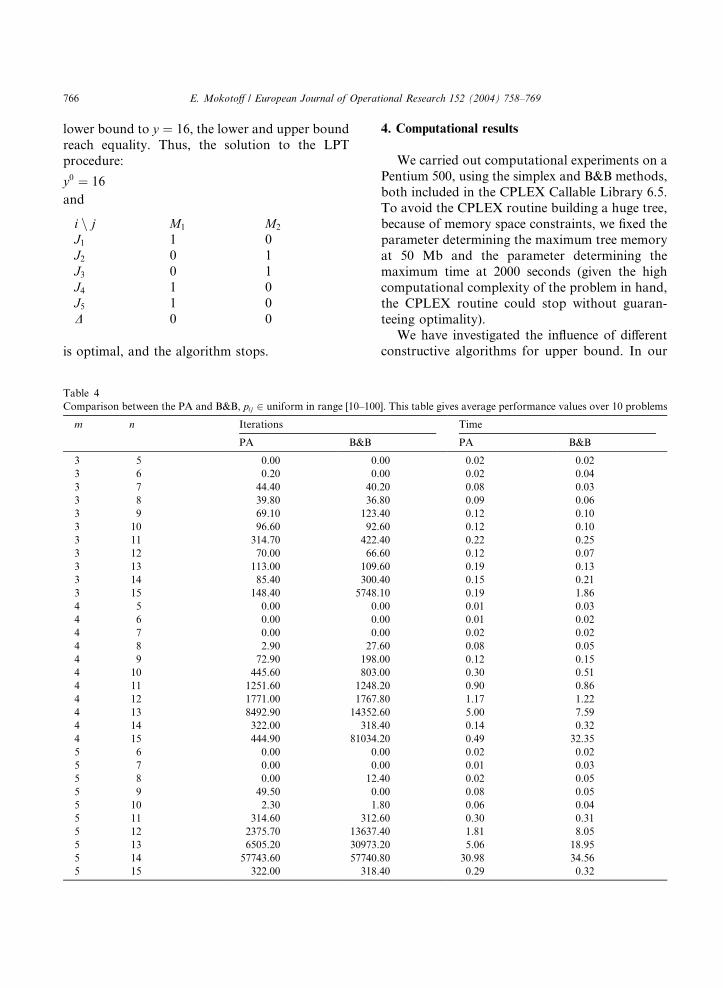
Table 4

Comparison between the PA and B&B, pij 2 uniform in range [10–100

m n Iterations

PA B&B

3 5 0.00 0.

3 6 0.20 0.

3 7 44.40 40.

3 8 39.80 36.

3 9 69.10 123.

3 10 96.60 92.

3 11 314.70 422.

3 12 70.00 66.

3 13 113.00 109.

3 14 85.40 300.

3 15 148.40 5748.

4 5 0.00 0.

4 6 0.00 0.

4 7 0.00 0.

4 8 2.90 27.

4 9 72.90 198.

4 10 445.60 803.

4 11 1251.60 1248.

4 12 1771.00 1767.

4 13 8492.90 14352.

4 14 322.00 318.

4 15 444.90 81034.

5 6 0.00 0.

5 7 0.00 0.

5 8 0.00 12.

5 9 49.50 0.

5 10 2.30 1.

5 11 314.60 312.

5 12 2375.70 13637.

5 13 6505.20 30973.

5 14 57743.60 57740.

5 15 322.00 318.

4. Computational results

We carried out computational experiments on a

Pentium 500, using the simplex and B&B methods,

both included in the CPLEX Callable Library 6.5.To avoid the CPLEX routine building a huge tree,

because of memory space constraints, we fixed the

parameter determining the maximum tree memory

at 50 Mb and the parameter determining the

maximum time at 2000 seconds (given the high

computational complexity of the problem in hand,

the CPLEX routine could stop without guaran-

teeing optimality).We have investigated the influence of different

constructive algorithms for upper bound. In our

]. This table gives average performance values over 10 problems

Time

PA B&B

00 0.02 0.02

00 0.02 0.04

20 0.08 0.03

80 0.09 0.06

40 0.12 0.10

60 0.12 0.10

40 0.22 0.25

60 0.12 0.07

60 0.19 0.13

40 0.15 0.21

10 0.19 1.86

00 0.01 0.03

00 0.01 0.02

00 0.02 0.02

60 0.08 0.05

00 0.12 0.15

00 0.30 0.51

20 0.90 0.86

80 1.17 1.22

60 5.00 7.59

40 0.14 0.32

20 0.49 32.35

00 0.02 0.02

00 0.01 0.03

40 0.02 0.05

00 0.08 0.05

80 0.06 0.04

60 0.30 0.31

40 1.81 8.05

20 5.06 18.95

80 30.98 34.56

40 0.29 0.32


experiment we have tried with LPT [2], MultiFit

with 7 and 17 iterations [1], improvement heuris-

tics with fixed gap with one iteration (FGH1) [10]

and the constructive algorithms with partial sets of

machines presented in [3].

The test problems obtained, randomly gener-ating the pi values according to uniform distribu-

tions in the range [1–100] for instances of varying

size, have been solved by the PA using the different

constructive algorithms to compute the upper

bound. Results for MultiFit with 7 iterations was

notably dominated by MultiFit with 17 iterations

(MF17). Among the constructive algorithms pre-

sented in [3] similar results were attained, so we

Table 5

Comparison between the PA and B&B, pij 2 uniform in range [50;100

m n Iterations

PA B&B

3 5 0.00 0

3 6 2.60 0

3 7 56.40 52

3 8 76.00 72

3 9 34.00 40

3 10 317.20 313

3 11 952.50 1124

3 12 251.70 591

3 13 2788.30 4000

3 14 3095.10 5675

3 15 188.50 95750

4 5 0.00 0

4 6 0.00 0

4 7 1.50 0

4 8 4.60 0

4 9 432.40 429

4 10 1175.50 1357

4 11 1428.00 1424

4 12 957.00 971

4 13 32442.40 32437

4 14 79954.30 109046

4 15 80362.70 154953

5 6 0.00 0

5 7 0.00 0

5 8 2.00 0

5 9 4.00 0

5 10 5.80 1

5 11 10174.80 10171

5 12 31845.80 31841

5 13 115404.60 115400

5 14 63308.80 63304

5 15 109050.80 119063

report the results corresponding to the partition

into 10 subsets and where d ¼ 80% (AP10(0.80)).

For different values of n and m, the entries in Table

1 give the average CPU time in seconds required

by the PA when using each of the algorithms,

computed over 10 problem instances. To evaluatethe incidence of refined upper bound in the cutting

plane phase, we present Table 2 which gives the

average over 10 problem instances of CPU time in

seconds required by the PA when using each of the

algorithms without taking into account the time

required to compute the upper bound. The results

shows that the AP10(0.80) gives slightly better

upper bound values than the others with difficult

]. This table gives average performance values over 10 problems

Time

PA B&B

.00 0.06 0.02

.00 0.06 0.01

.80 0.10 0.03

.40 0.12 0.09

.20 0.11 0.07

.60 0.22 0.16

.00 0.54 0.53

.80 0.38 0.37

.80 1.38 1.56

.60 1.48 2.54

.10 0.27 7.64

.00 0.01 0.02

.00 0.07 0.03

.00 0.05 0.04

.00 0.12 0.04

.20 0.25 0.20

.80 0.74 0.78

.20 0.99 0.96

.60 0.95 0.88

.60 15.74 15.55

.60 39.84 52.24

.10 47.06 87.77

.00 0.01 0.03

.00 0.03 0.03

.60 0.04 0.04

.00 0.02 0.02

.00 0.06 0.06

.40 3.61 3.61

.60 17.96 17.96

.20 74.23 74.55

.60 50.04 53.34

.60 52.73 95.20

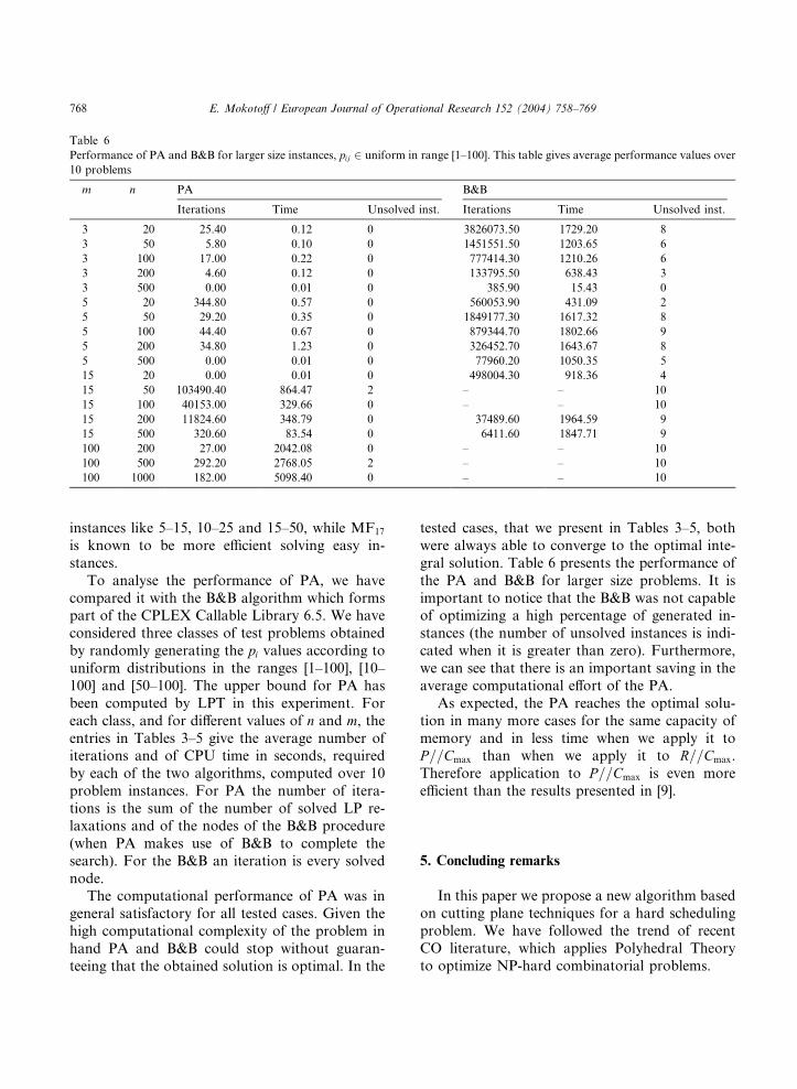
Table 6

Performance of PA and B&B for larger size instances, pij 2 uniform in range [1–100]. This table gives average performance values over

10 problems

m n PA B&B

Iterations Time Unsolved inst. Iterations Time Unsolved inst.

3 20 25.40 0.12 0 3826073.50 1729.20 8

3 50 5.80 0.10 0 1451551.50 1203.65 6

3 100 17.00 0.22 0 777414.30 1210.26 6

3 200 4.60 0.12 0 133795.50 638.43 3

3 500 0.00 0.01 0 385.90 15.43 0

5 20 344.80 0.57 0 560053.90 431.09 2

5 50 29.20 0.35 0 1849177.30 1617.32 8

5 100 44.40 0.67 0 879344.70 1802.66 9

5 200 34.80 1.23 0 326452.70 1643.67 8

5 500 0.00 0.01 0 77960.20 1050.35 5

15 20 0.00 0.01 0 498004.30 918.36 4

15 50 103490.40 864.47 2 – – 10

15 100 40153.00 329.66 0 – – 10

15 200 11824.60 348.79 0 37489.60 1964.59 9

15 500 320.60 83.54 0 6411.60 1847.71 9

100 200 27.00 2042.08 0 – – 10

100 500 292.20 2768.05 2 – – 10

100 1000 182.00 5098.40 0 – – 10


instances like 5–15, 10–25 and 15–50, while MF17

is known to be more efficient solving easy in-

stances.

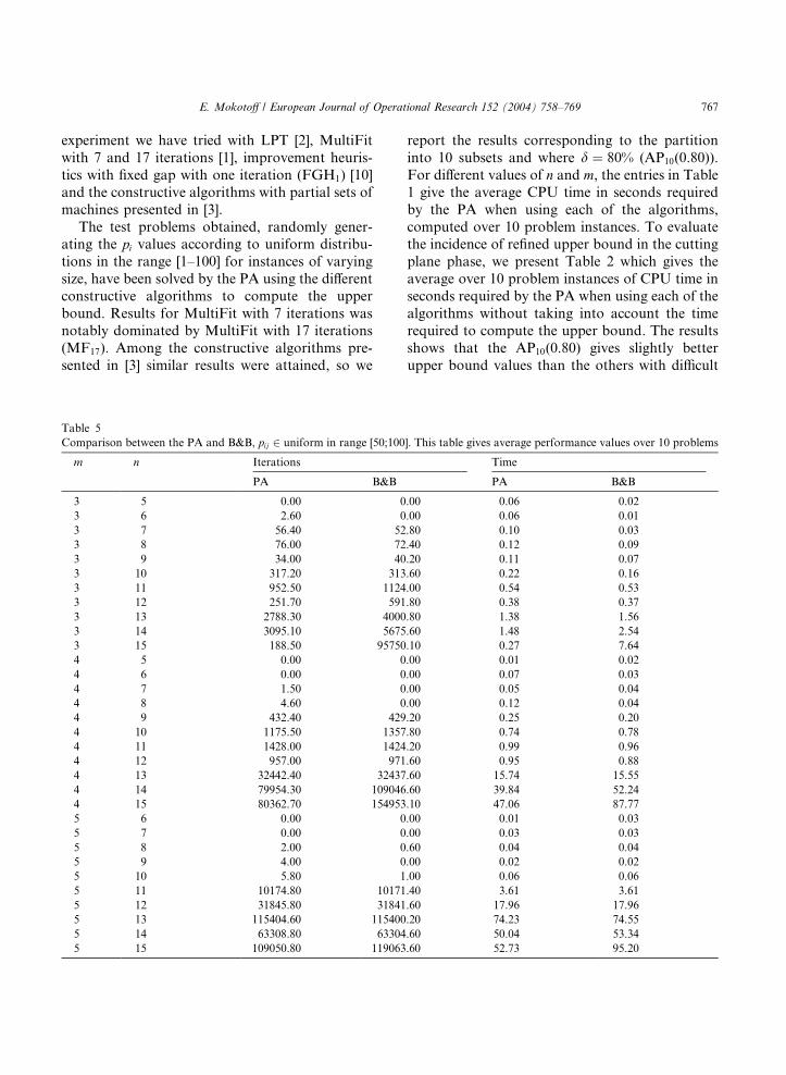
To analyse the performance of PA, we have

compared it with the B&B algorithm which formspart of the CPLEX Callable Library 6.5. We have

considered three classes of test problems obtained

by randomly generating the pi values according to

uniform distributions in the ranges [1–100], [10–

100] and [50–100]. The upper bound for PA has

been computed by LPT in this experiment. For

each class, and for different values of n and m, theentries in Tables 3–5 give the average number ofiterations and of CPU time in seconds, required

by each of the two algorithms, computed over 10

problem instances. For PA the number of itera-

tions is the sum of the number of solved LP re-

laxations and of the nodes of the B&B procedure

(when PA makes use of B&B to complete the

search). For the B&B an iteration is every solved

node.The computational performance of PA was in

general satisfactory for all tested cases. Given the

high computational complexity of the problem in

hand PA and B&B could stop without guaran-

teeing that the obtained solution is optimal. In the

tested cases, that we present in Tables 3–5, both

were always able to converge to the optimal inte-

gral solution. Table 6 presents the performance of

the PA and B&B for larger size problems. It is

important to notice that the B&B was not capableof optimizing a high percentage of generated in-

stances (the number of unsolved instances is indi-

cated when it is greater than zero). Furthermore,

we can see that there is an important saving in the

average computational effort of the PA.

As expected, the PA reaches the optimal solu-

tion in many more cases for the same capacity of

memory and in less time when we apply it toP==Cmax than when we apply it to R==Cmax.

Therefore application to P==Cmax is even more

efficient than the results presented in [9].

5. Concluding remarks

In this paper we propose a new algorithm based

on cutting plane techniques for a hard scheduling

problem. We have followed the trend of recent

CO literature, which applies Polyhedral Theory

to optimize NP-hard combinatorial problems.


The obtained results show that this kind of

approach is quite a powerful tool for effectively

producing quality feasible solutions. They also

give support to the hypothesis stating that spe-

cially-developed algorithms for specific combina-

torial problems work better than general methodslike B&B.

After having applied this technique to P==Cmax

and R==Cmax, and having refined the computation

of initial lower and upper bound, we have been

able to prove the efficiency of this algorithm and

thus we are now considering the development of

similar approaches to solve even harder scheduling

problems such as job-shop problems.

References

[1] E.G. Coffman Jr., M.R. Garey, D.S. Johnson, An appli-

cation of Bin-Packing to multiprocessor scheduling, SIAM

Journal on Computing 7 (1978) 1–17.

[2] R.L. Graham, Bounds on the performance of scheduling

algorithms, SIAM Journal on Applied Mathematics 17

(1969) 263–269.

[3] J.L. Jimeno, E. Mokotoff, J. P�eerez, A constructive algo-

rithm to minimise the makespan on identical parallel

machine, in: Eighth International Workshop on Project

Management and Scheduling, Valencia, 2002.

[4] M. J€uunger, G. Reinelt, S. Thienel, Practical problem

solving with cutting plane algorithms in combinatorial

optimization, in: W. Cook, L. Lov�aasz, P. Seymour (Eds.),

Combinatorial Optimization, Dimacs, Vol. 20, 1995, 111–

152.

[5] J.K. Lenstra, A.H.G. Rinnooy Kan, Computational com-

plexity of discrete optimization, in: J.K. Lenstra, A.H.G.

Rinnooy Kan, P. Van Emde Boas (Eds.), Interfaces

between Computer Science and Operations Research,

Proceedings of a Symposium held at the Matematisch

Centrum, Amsterdam, 1979, 64–85.

[6] R. McNaughton, Scheduling with deadlines and loss

function, Management Science 6 (1959) 1–12.

[7] E. Mokotoff, Parallel machines scheduling problems: A

survey, Asia-Pacific Journal of Operational Research 18

(2001) 193–242.

[8] E. Mokotoff, Scheduling to minimize the makespan on

identical parallel machines: An LP-based algorithm, In-

vestigaci�oon Operativa 8 (1999) 97–108.

[9] E. Mokotoff, P. Chr�eetienne, A cutting plane algorithm for

the unrelated parallel machine scheduling problem, Euro-

pean Journal of Operational Research 141 (2002) 517–527.

[10] E. Mokotoff, J.L. Jimeno, A. Guti�eerrez, List scheduling

algorithms to minimize the makespan on identical parallel

machines, Top 9 (2001) 243–269.

[11] W.R. Pulleyblank, Polyhedral Combinatorics, in: J.L.

Nemhauser, A.H.G. Rinnooy Kan, M.J. Todd (Eds.),

Handbooks in Operations Research and Management

Science 1: Optimization, 1989, pp. 371–446.

[12] T. Van Roy, L. Wolsey, Valid inequalities for mixed 0-1

programs, Discrete Applied Mathematics 4 (1986) 199–

213.

Documents

An exact algorithm for the identical parallel machine scheduling problem