Embed Size (px)
Citation preview
Wayne State University
Wayne State University Dissertations
1-1-2011
An integrated decision support framework forremanufacturing in the automotive industryAkhilesh KumarWayne State University,
Follow this and additional works at: http://digitalcommons.wayne.edu/oa_dissertations
Part of the Business Administration, Management, and Operations Commons, and the IndustrialEngineering Commons
This Open Access Dissertation is brought to you for free and open access by DigitalCommons@WayneState. It has been accepted for inclusion inWayne State University Dissertations by an authorized administrator of DigitalCommons@WayneState.
Recommended CitationKumar, Akhilesh, "An integrated decision support framework for remanufacturing in the automotive industry" (2011). Wayne StateUniversity Dissertations. Paper 316.
AN INTEGRATED DECISION SUPPORT FRAMEWORK FOR
REMANUFACTURING IN THE AUTOMOTIVE INDUSTRY
by
AKHILESH KUMAR
DISSERTATION
Submitted to the Graduate School
of Wayne State University,
Detroit, Michigan
in partial fulfillment of the requirements
for the degree of
DOCTOR OF PHILOSOPHY
2011
MAJOR: INDUSTRIAL ENGINEERING
Approved by:
______________________________________
Advisor Date
______________________________________
______________________________________
______________________________________

ii
DEDICATION
To my parents, Mrs. Shanti Ray and Mr. Birda Ray

iii
ACKNOWLEDGEMENTS
First and foremost I would like to thank my PhD advisor Prof. Ratna Babu Chinnam.
Without his inspirational guidance, enthusiasm, and encouragements this feat would not
have been possible. My special thanks go to my committee members Prof. Richard Darin
Ellis, Prof. Alper E Murat and Prof. John C Taylor for their suggestion for improvement.
I am very grateful to present chair Prof. Leslie Monplaisir and ex-chair Prof. Kenneth
Chelst for their support and enthusiasm to accomplish this goal.
I would also thank Mr. Ramesh Subramoniam of Delphi Corporation for providing the
test datasets for my research. Thanks to my friends at ISE department, especially Dr. P.
Baruah, Mr. D. Cao, Dr. R Govindu, and Mrs. Ucar, for their help and support.
Talking about my research, I cannot forget to thanks my mentor Prof. M. K. Tiwari. He
channelized my energy towards this pious profession and guided me to attain the maturity
required to pursue a meaningful research.
Lastly, I would like to thank my brothers Mr. R. Kumar and Mr. K. Kumar and my sister
Mrs. P. Roy. Their endless love and support made it possible to complete this study.
iv
TABLE OF CONTENTS
Dedication .......................................................................................................................... ii
Acknowledgements .......................................................................................................... iii
List of Tables .................................................................................................................... vi
List of Figures .................................................................................................................. vii
Chapter 1 : INTRODUCTION ........................................................................................ 1
1.1 Research Setting ........................................................................................................ 3
1.2 Research Objectives .................................................................................................. 6
1.3 Research Scope ......................................................................................................... 7
REFERENCES ................................................................................................................ 8
Chapter 2 : STRATEGIC CAPACITY PLANNING AND MANAGEMENT OF
REMANUFACTURED PRODUCTS ............................................................................. 9
2.1 Related Literature ................................................................................................... 12
2.2 Capacity Planning Model ........................................................................................ 16
2.2.1 Base Case without Remanufacturing ................................................................ 16
2.2.2 Remanufacturing Case ...................................................................................... 17
2.2.3 Optimization Problem ....................................................................................... 22
2.3.1 Optimization of Policy Parameters ................................................................... 26
2.3.2 Structural Properties of the Optimal Policy ...................................................... 28
2.4. Numerical Investigation ......................................................................................... 30
2.4.1 Structural Properties of the Optimal Solution and Optimal Cost ..................... 31
2.4.2 Effect of Parameters on Optimal Time to Launch and Optimal Capacity ........ 39
2.5 Conclusion and Future Research ............................................................................. 46
REFERENCES .............................................................................................................. 48
v
APPENDIX ................................................................................................................... 52
Chapter 3 : HAZARD RATE MODELS FOR CORE RETURNS FORECASTING
IN REMANUFACTURING ........................................................................................... 55
3.2 Literature Review .................................................................................................... 57
3.3 The Modelling Framework...................................................................................... 60
3.3.1 Semi Parametric Modelling (Cox-proportional Hazard rate model) ................ 61
3.3.2 Parametric Modeling ........................................................................................ 64
3.4 Case Study ............................................................................................................... 64
3.4.1 Data ................................................................................................................... 65
3.4.2 Nomenclature .................................................................................................... 66
3. 5. Results and Discussion .......................................................................................... 66
3.5.1 Parameter Estimates ......................................................................................... 67
3.5.2 Validation ......................................................................................................... 68
3.5.2.1 Stability and Efficiency of the Estimates ...................................................... 70
3.5.2.2 Predictive Performance of the Models .......................................................... 72
3.5.3 An Important Note ............................................................................................... 74
3.6. Conclusions and Future Work ................................................................................ 78
REFERENCES .............................................................................................................. 79
Chapter 4 : CONCLUSION AND FUTURE RESEARCH......................................... 82
4.1 Future Research ....................................................................................................... 87
Abstract ............................................................................................................................ 89
Autobiographical Statement .......................................................................................... 92
vi
LIST OF TABLES
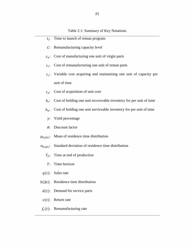
Table 2.1: Summary of Key Notations ............................................................................. 21
Table 2.2: Heuristic algorithm to compute optimal policy parameters and ......... 27
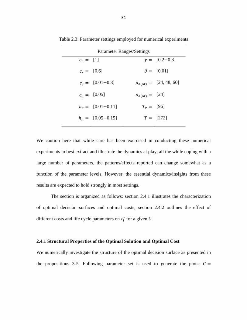
Table 2.3: Parameter settings employed for numerical experiments ................................ 31
Table 3.1 Covariate Estimates .......................................................................................... 68
Table 3.2 Estimated Coefficients and standardized measures of variability (I: Complete
dataset, II: Calibration-dataset, III: Validation-dataset) ................................ 71
Table 3.3 Hit Rates ........................................................................................................... 73
Table 3.4 Mean Square Error (MSE) in Forecast ............................................................. 73
Table 3.5 Estimates- Cox with Time-by-Covariate Interaction ........................................ 75
Table 3.6 Cox with Random Effect (Frailty Model) Estimates ........................................ 77
vii
LIST OF FIGURES
Figure 1.1 Typical production pattern of an automotive product considered for reman
over its life-cycle............................................................................................... 4
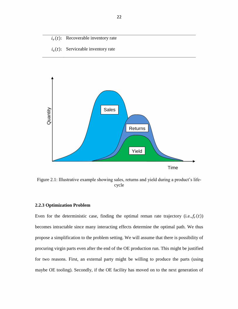
Figure 2.1: Illustrative example showing sales, returns and yield during a product‟s life-
cycle ................................................................................................................ 22
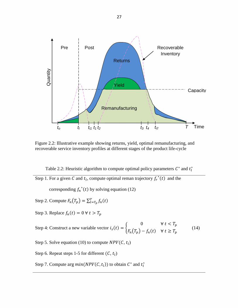
Figure 2.2: Illustrative example showing returns, yield, optimal remanufacturing, and
recoverable service inventory profiles at different stages of the product life-
cycle ................................................................................................................ 27
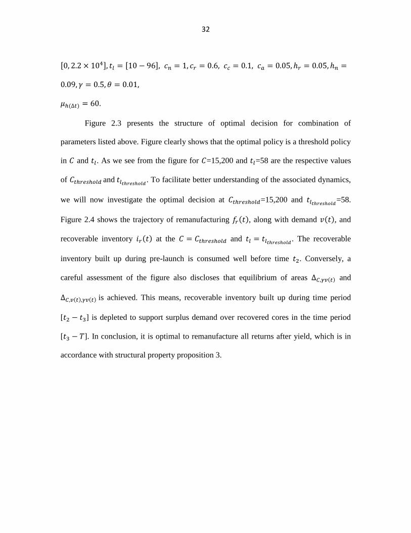
Figure 2.3: Optimal total reman volume as a function of and ................................... 33
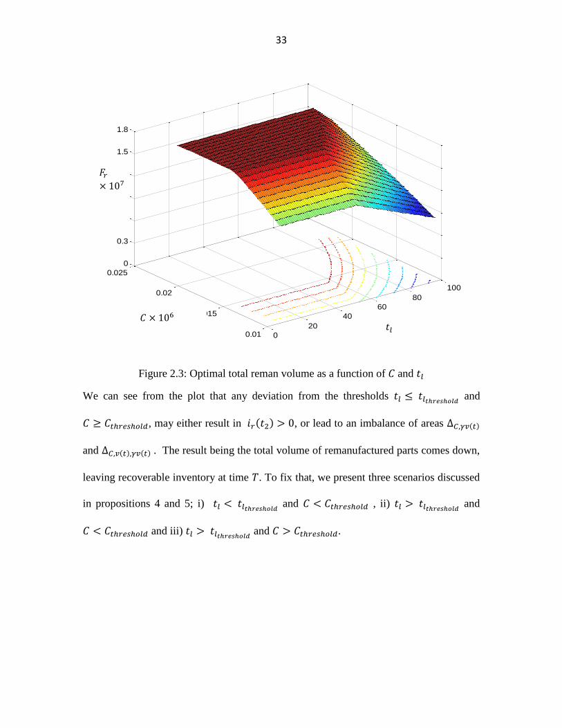
Figure 2.4: Trajectory of optimal states and control variables at and
................................................................................................... 34
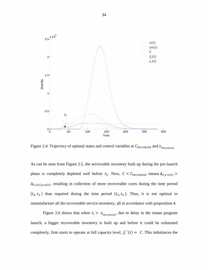
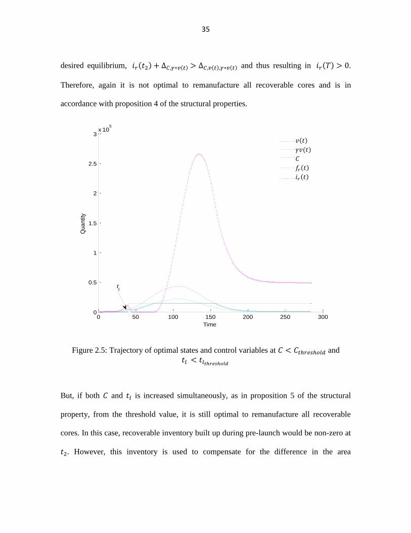
Figure 2.5: Trajectory of optimal states and control variables at and
.......................................................................................... 35
Figure 2.6: Trajectory of optimal states and control variables at and
.......................................................................................... 36
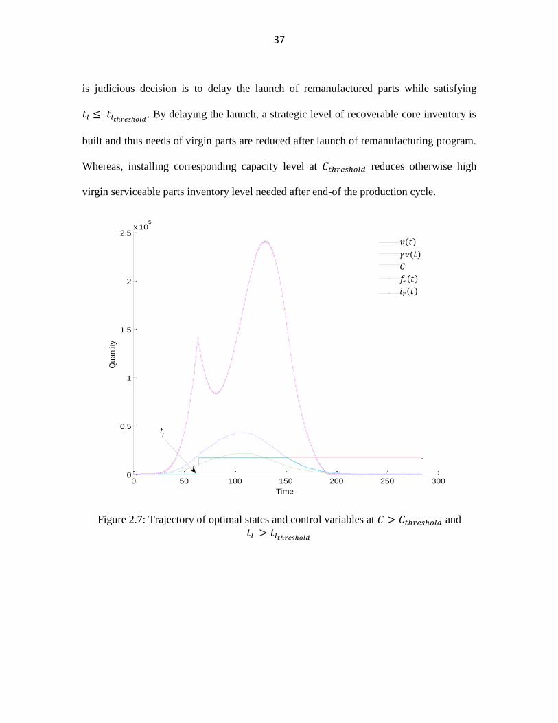
Figure 2.7: Trajectory of optimal states and control variables at and
.......................................................................................... 37
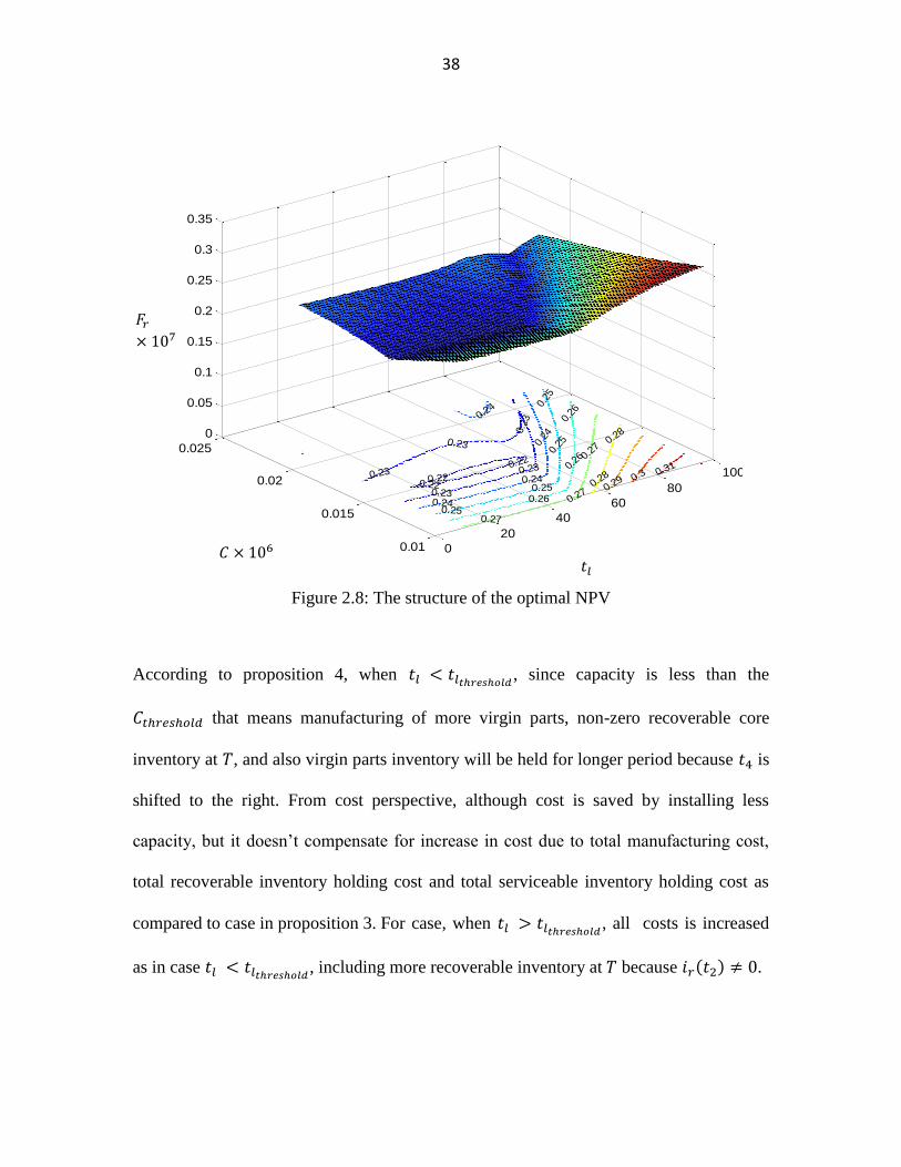
Figure 2.8: The structure of the optimal NPV .................................................................. 38
Figure 2.9: Effect of on , and %Rel. Savings ( ......... 41
Figure 2.10: Effect of on , and %Rel. Savings ( 42
Figure 2.11: Effect of on , and %Rel. Savings ( ..... 44
Figure 2.12: Effect of on , and %Rel. Savings ( ........... 45
Figure 2.13: Cumulative stochastic returns with randomness in mean of 0.6 .................. 46
viii
Figure 3.1 History of Core Return Delays for a Delphi Product Family (Source: Delphi).
Note: Red line at -450 slope denotes censoring time (i.e., date for termination
of data collection). .......................................................................................... 65
Figure 3.2 Expected return behavior of customers using Cox‟ model ............................. 69
Figure 3.3 Baseline Survival Plot ..................................................................................... 74
Figure 3.4 Effective β for different time periods .............................................................. 76
1
Chapter 1 : INTRODUCTION
In today‟s global economy, firms are seeking any and every possible opportunity to
differentiate themselves from competitors, to reduce their costs, and to add value to their
supply chains and end customers. One increasingly popular option, under growing
consumer awareness and increasing legislation, is to reintegrate used or returned product
into the supply chain to regain the materials for economic and sustainability purposes
(Schultmann et al., 2006). An important class of such “reverse” goods flows has to do
with remanufacturing, which refers to activities that restore used products or their major
modules to operational condition for use in place of new product or for other channels
(e.g., spare parts). U.S. Environmental Protection Agency (EPA) advocates the practice
of remanufacturing as economical, energy-efficient and environmentally friendly
approach to reduce industrial waste (US EPA, 1997). Another important reason for
improving reverse logistics is to cope with returns that have become endemic in many
industries. For example, according to a recent Consumer Electronics Industry survey by
the Reverse Logistics Executive Council, the average return rate is 8.46% in the high-
tech industry (Thrikutam and Kumar - infosys.com 2004), with return rates as high as
20% for certain product segments. The value of these returned consumer electronic goods
in the U.S. is estimated at $104B for 2004 with the cost of managing the returns running
around $8B. While there are several types of returns (commercial returns, repairable
returns, end-of-use returns, end-of-life returns, recalls, and others …), the 8.46% return
rate mostly covers commercial returns (that occur in the sales phase or shortly after) with
immediate demand at another market location or segment. While efficient management of
2
commercial returns is challenging and necessary, particularly given the growth in return
rates, remanufacturing is often far more complex. It not only deals with other types of
returns that bring about lot more uncertainties (e.g., timing/location of return, return
volume, quality), but also have to address complexities associated with reman production
planning and control. Remanufacturing has traditionally been prevalent in such industries
as automotive, electrical equipment, furniture, machinery, tires, and toner cartridges.
In the automotive industry, production parts can be roughly divided into Original
Equipment (OE) parts and Aftermarket parts. OE parts refer to parts used in producing
new vehicles, whereas, aftermarket parts refers to parts traded after original equipment
sale, which includes both OE service (for parts under OEM warranty) and independent
aftermarket (IAM) services. The automotive aftermarket industry is estimated at $198B
annually in the US, with IAM sales estimated at $142B, mostly from collision centers and
independent mechanics1. While the remanufacturing business was traditionally
dominated by IAM companies, hefty profit margins and growing pressures to improve
corporate citizenship, are encouraging more and more OEM and tier-1 suppliers to pursue
remanufacturing. According to a recent survey by Inmar (Inmar, Special Report 2009), in
the automotive industry, return rates are known to vary between 5%-25%. Survey also
identifies various factors leading to poor returns: 1) Poor information flow, 2) Multiple
networks that poorly interface with one another, 3) Different part numbering schemes for
the same replacement parts, 4) Data entry order errors, 5) Incorrect shipments, 6) Mis-
diagnosis, 7) Over ordering , and 8) Defective parts. Given returns and the size of the
1 http://www.oealliance.com/industry.htm
3
aftermarket business, there are tremendous opportunities for OEMs and suppliers to
engage in remanufacturing business to improve profitability and sustainability.
While all these opportunities abound, key complications for OEMs and suppliers
is the difficulty in making decisions related to launch of remanufacturing program and
efficient management of remanufacturing operations and logistics. There is lack of a
structured and holistic decision support framework, which can guide firms in decision
making related to timing the launch of the remanufacturing program, capacity
installation/management etc. Further, efficient production and inventory management of
remanufacturing parts for the supplier heavily impinges on the ability to accurately
forecast these core returns from customers (besides forecasting demand for
remanufacturing parts and securing cores from the open market, as necessary). All these
factors are motivation for the proposed research.
1.1 Research Setting
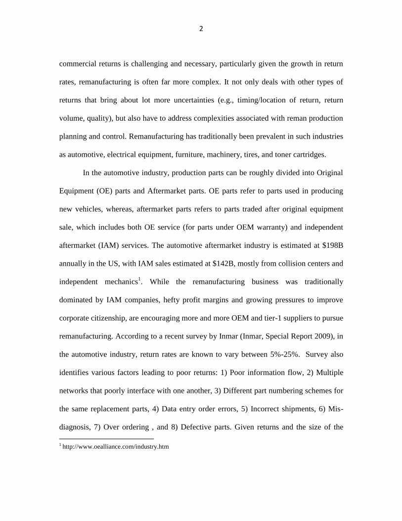
For a typical automotive product targeted for reman, production during its life-cycle can
be roughly divided into three phases. Phase I more or less deals with the production of
OE parts to support demand for new OEM product and tends to be relatively high volume
production. Phase II covers the period of transition from production of just OE parts to
both OE and OE service (OES) parts production and eventually just OE service and the
independent after-market (IAM). Phase III covers the production of parts for just the
IAM. Phase 0, preceding all the production phases, encompasses the various phases of
product development with considerations for remanufacturing.
4
Figure 1.1 Typical production pattern of an automotive product considered for reman
over its life-cycle
Figure 1.1 illustrates these phases along with representative production levels. For firms
that do not engage in IAM or reman, in the automotive industry, the product from the end
of the OE production cycle is often stocked to meet the 15 years spare-parts availability
requirement.
For firms that engage in OE production as well as remanufacturing, the second and third
phases impose new challenges apart from traditional forward supply chain management.
In other words, presence of reverse logistic flows in a supply chain magnifies the
variability and its effects. Following are the remanufacturing decision making needs
during these different phases.
Phase 0: At this phase firms need to establish the business case for remanufacturing
depending on the product attributes. This will trigger product development for
remanufacturing.
Phase I Phase II
Phase 0
Phase III
5
Phase I: During OE production, firms need to establish contracts with dealers and third
party collectors of “cores” or used product to establish return flow channels.
Phase II: At this stage, firms need to evaluate various decisions. Whether to launch
remanufacturing program or keep producing only OE parts to meet new all demand?
Decision to launch remanufacturing program depends among other things (e.g., potential
margins) the product life cycle, demand pattern for new product, demand pattern for
reman product, and availability/reliability of core returns. If firm decides to launch a
reman program for the product under consideration, then decisions need to be taken on
the timing of the program launch and reman capacity installation and management. In
addition, since firm is in a hybrid production state (involving both manufacturing and
remanufacturing), production planning and control becomes crucial because material
flows from both the channels are dependent on each other. It should be noted here that
core returns for OE service parts are often very reliable for they involve a fast trading
cycle. The cycle is initiated with the receipt of a core or defective unit by the supplier
from the dealer followed by an often overnight or same day delivery of a reman unit to
the dealer from very limited finished goods inventory (FGI). The supplier then remans
the core (often the same day) and stocks the unit for the next cycle. Given the cycle
speed, the OE remanufacturing activity can be relatively efficient, at least from the
perspective of core inventory and reman FGI.
Phase III: Decisions at this phase are similar to Phase II decisions. Here, high volume OE
production is over. Firms need to make decision over launching remanufacturing program
for IAM, if not done during Phase II. Depending on the returns from warranty claims,

6
firms either can launch the remanufacturing for IAM along with reman parts for OE
service or wait for more core returns and establishment of core supply contracts with
independent collectors. The major difference from Phase II is the significant uncertainty
in core returns. Unlike the OE service setting, the trade in process is often not initiated
with the receipt of a core but with an order. The reman product is shipped to the customer
along with an RMA for the cores and a core charge (customer will not be reimbursed for
the core charge until the cores are returned). However, our experience with a major Tier-
1 supplier shows that customers can take months and even years to return cores. Hence,
inventory management (of cores as well as FGI) becomes more critical as well as overall
production planning and control.
1.2 Research Objectives
The objective of this thesis is to develop an integrated framework, for industries
supporting OE, OES and IAM business, to guide transition from OE production to hybrid
settings. The specific objectives are as follows:
1. To develop models that can facilitate better timing of the launch of remanufacturing
program for OE service and IAM and reman capacity planning. This is of particular
concern to our collaborator Delphi Automotive LLP. While the literature offers no
guidance/models, there are risks associated with both premature launch (reman OES parts
are priced differently and the absence of reliable core supply due to premature launch can
force the supplier to provide virgin parts in place of reman parts and poor utilization of
reman capacity) or delayed launch (lost opportunity of provide reman product).
7
2. To develop a modelling framework for core-return forecasting to facilitate decision-
making at different phases. The prerequisites for this objective are:
Ability to forecast core returns for product as well as product families; A key
requirement here is the ability of the modelling framework to support data
sparsity (a lesson learnt from our work with Delphi Automotive LLP)
Ability to forecast when there is long lag between product shipment/sale and core
return
Ability to support/exploit different levels/sets of information regarding historical
sales, return rates, market inventory etc.
Ability to provide feedback to timing the launch of a new product
remanufacturing program and reman capacity planning
1.3 Research Scope
In this dissertation, we assume that the business case for remanufacturing has already
been established by the firm. Thus, our study will focus on developing an integrated
framework for decision support during phases II of the production life-cycle (see Figure
1.1). In this dissertation, we have considered phase II and III jointly.
Scope of this work includes new models for core return, timing the launch of a
remanufacturing program, and capacity planning. We have validated the overall
framework and the associate models and methods through case studies with Delphi.
8
The rest of the dissertation is organized as follows. Chapter 2 presents strategic capacity
management of remanufacturing. Chapter 3 offers models for core-returns forecasting.
Finally, Section 4 presents conclusion and future research directions.
REFERENCES
Inmar CLS Reverse Logistics, October 2009. Special Report: Automotive Aftermarket
Reverse Logistics Opportunities, MEMA MIS Council, Inmar.
Schultmann, F., Zumkeller M., & Rentz O., 2006. Modeling reverse logistic tasks within
closed-loop supply chains: an example from the automotive industry, European Journal
of Operational Research, 171- 3, 1033-1050.
Thrikutam, P., and Kumar, S., 2004, Turning Returns Management in to a Competitive
Advantage in Hi-Tech Manufacturing, infosys.com
United States Environmental Protection Agency, 1997. Remanufactured products: Good
as new. EPA530-N-002.
9
Chapter 2 : STRATEGIC CAPACITY PLANNING AND MANAGEMENT
OF REMANUFACTURED PRODUCTS
Strategic capacity planning plays an important role in the effective management of
product life-cycles and improving their profitability. In particular, decisions related to
determining the sizes and timing of capacity investments. To effectively decide on
„timing the launch’, a firm must tradeoff the cost of capacity, supply, and inventories,
with the revenues from the product demand over its life cycle. In addition, firm needs to
make an important decision at the operations level on „how much capacity to install’.
These decisions impose more challenges for firms that engage in original equipment (OE)
production as well as remanufacturing. The presence of reverse logistic flows magnifies
the variability in a supply chain due to uncertainty in timing/location of returns, return
volume, quality etc. In other words, the timing and volume of used product returns are
binding supply constraints for remanufacturing. Capacity management is, thus, even
more complex and critical for supply chains that involve reverse logistics and
remanufacturing.
The original motivation for our research came from the request of a leading global
tier-1 automotive supplier, Delphi Automotive LLP, engaged in OE production as well as
providing products to the aftermarket (both for OE service and the independent
aftermarket). Key complications faced by the company were the difficulties in making
decisions relating to proper timing of the launch of the reman product program, capacity
installation, and efficient management of remanufacturing operations and logistics.
Overall, there is recognition for the lack of a structured and holistic decision support
10
framework that can guide firms in decision making related to both, timing the launch of
the remanufacturing program and capacity installation/management.
For a typical automotive product, production during its life cycle can be roughly
divided into two phases. Phase I deals with the production of OE parts to support demand
for new OEM product and tends to be relatively high volume production. Phase II covers
the period of transition from OE parts to both OE parts and service parts including both
OE service parts (OES) and eventually independent aftermarket (IAM) demand too. At
the end of the regular production cycle, firms usually make a last run production to stock
parts to meet the spare-parts availability requirement (in the US, the legal requirement is
15 years from the end of production
One increasingly popular option to support aftermarket demand (partially or fully)
has to do with remanufacturing. For firms that engage in OE parts production as well as
remanufacturing to support aftermarket services (as is the case with our collaborator,
Delphi), it is seldom optimal to start the reman product program with the start of the
earliest core returns. The reason being, in the absence of a reliable core supply for
remanufacturing due to a premature reman product launch, the supplier is forced to
provide new or virgin parts in place of reman parts to cover demand for reman product
that exceeds reman production and inventory, a costly affair and in addition results in
poor utilization of remanufacturing capacity. Therefore, it is more common for firms to
delay the start of the reman program to the end of the OE production cycle. By delaying
the launch to the end of the OE production cycle, firm can accumulate enough core
returns to build up a large strategic recoverable inventory. This helps in better utilization
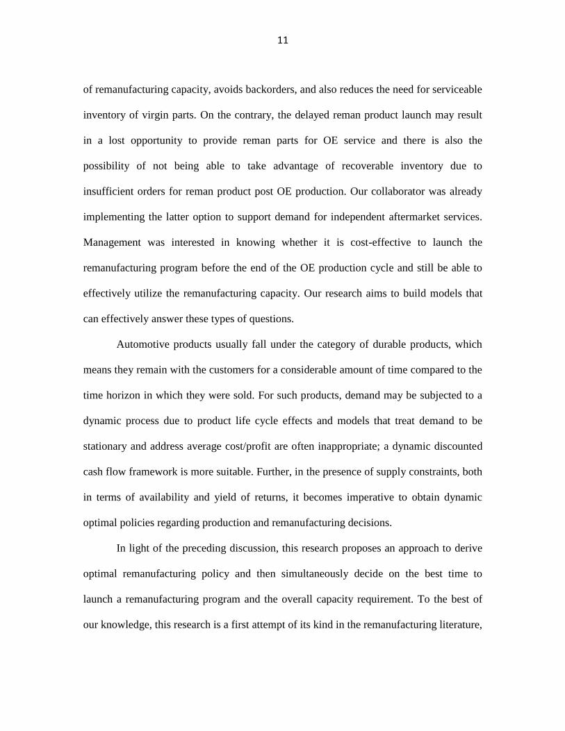
11
of remanufacturing capacity, avoids backorders, and also reduces the need for serviceable
inventory of virgin parts. On the contrary, the delayed reman product launch may result
in a lost opportunity to provide reman parts for OE service and there is also the
possibility of not being able to take advantage of recoverable inventory due to
insufficient orders for reman product post OE production. Our collaborator was already
implementing the latter option to support demand for independent aftermarket services.
Management was interested in knowing whether it is cost-effective to launch the
remanufacturing program before the end of the OE production cycle and still be able to
effectively utilize the remanufacturing capacity. Our research aims to build models that
can effectively answer these types of questions.
Automotive products usually fall under the category of durable products, which
means they remain with the customers for a considerable amount of time compared to the
time horizon in which they were sold. For such products, demand may be subjected to a
dynamic process due to product life cycle effects and models that treat demand to be
stationary and address average cost/profit are often inappropriate; a dynamic discounted
cash flow framework is more suitable. Further, in the presence of supply constraints, both
in terms of availability and yield of returns, it becomes imperative to obtain dynamic
optimal policies regarding production and remanufacturing decisions.
In light of the preceding discussion, this research proposes an approach to derive
optimal remanufacturing policy and then simultaneously decide on the best time to
launch a remanufacturing program and the overall capacity requirement. To the best of
our knowledge, this research is a first attempt of its kind in the remanufacturing literature,
12
as prior research treated these interrelated decisions separately. The primary focus of this
study is to develop intuition for drivers of cost-efficient remanufacturing program for
aftermarket services while taking life-cycle dynamics into account. The insights are
obtained by minimizing the discounted cash outflows caused by appropriate investment
and return inventory building decisions. Though a simplistic deterministic sales and
return dynamics are analyzed, our analysis of stochastic returns scenario revealed that
proposed deterministic approach is sufficient enough to capture the important dynamics
of cost-effective remanufacturing programs.
Remainder of this chapter is organized as follows: Section 2.1 outlines related
literature. Proposed model is discussed in section 2.2. Numerical investigation is
presented in Section 2.3. Finally, conclusion and future research in section 2.4.
2.1 Related Literature
There is a vast body of literature dealing with operational issues of decision making in
reverse logistics e.g. material resource planning (Ferrer and Whybark (2001), scheduling
and shop floor management (Guide et al. 1997, 1998), inventory control (Van der Laan et
al. 1999, Toktay et al. 2000), logistic network design (Fleischmann 2001), and routing
(Beullens 2001). We encourage readers to refer a recent survey by Ilgin and Gupta (2010)
for detailed overview of this literature. In contrast, today, the important problems of
business are not tactical or operational but tend to be strategic and mostly unstructured
(Guide, 2006). According to Valchos (2007), despite considerable emphasis over the last
decade on long-term strategic management problems in reverse logistics, there are almost
13
no studies in the literature thus far. Further, one of the most influential aspects of
investment decision, financial justification has widely been neglected in most of the
studies (Kleber 2006).
Most of the research considering strategic issues in reveres logistics have been
confined to network design in a single-period (see, e.g. Barros et al. 1998; Louwers et al.
1999) and less commonly a multi-period (Realff et al. 2004) setting with given product
characteristics. Shih (2001) studied reverse logistics planning for electronic products in
Taiwan. Using historical data, the author presented a model to determine the optimal
capacity expansion plans of storage and disassembly facilities for different product take-
back rates. Franke et al. (2005) developed a model for mobile phone remanufacturing to
determine the required capacities for remanufacturing operations. They used information
about uncertainties in the amount and conditions of returns as well as combinatorial
optimization to determine the capacities of work stations. Francas (2009) developed a
network configuration model for a multi-product supply chain in which a firm
manufactures new products and remanufactures used products. Built on a stochastic
programming approach that accounts for uncertainty in demand and returns, they studied
capacity investment from a newsvendor network perspective and compare the
performance of simultaneous and sequential design. Ryan (2010) developed a single-
period model for capacity planning that determines the optimal amount of expansion for
different lead times to obtain remanufacturing capacity. They stated that the difference
between their research and past work is that they focus jointly on the forecasting and
capacity management of returned products. Mutha (2010) presented a mathematical
14
model for handling product returns. The focus is on deciding the number of facilities,
their locations and allocation of corresponding flow of used products and modules at an
optimal cost for a given market demand and used product returned quantities. In all these
approaches, the decision at which time to set up the respective facilities has already been
made or facilities were already in place.
One major stream of capacity planning research in the reverse logistics domain is
based on System Dynamics (SD) modeling. Georgiadis et al. (2003) introduce
systematically the use of SD methodology in the analysis of closed-loop supply chains
(CLSCs). They use a set of level of remanufacturing and collection capacities to study the
effect of environmental issues on reverse channel‟s activities. Georgiadis and Vlachos
(2004) further extend that SD model to account for environmental issues such as „„green
image” and effect of „„take-back obligation” on product flows in the reverse channel,
while considering the capacity levels exogenously. Vlachos et al. (2007) study capacity
expansion policies in the reverse channel of a CLSC with remanufacturing activities
assuming stationary demand, hence ignoring the concept of a limited product lifecycle
and issues related to capacity contraction. Georgiadis et al. (2006) make a first attempt
towards a more holistic approach, developing an SD model for a single product CLSC
with remanufacturing activities in the reverse channel. They analyze the capacity
planning policies both for collection and remanufacturing activities in the reverse
channel, assuming that demand may follow different but standard lifecycle patterns
consisting of the introduction, growth, maturity and decline stages. Specifically, they
investigate how the lifecycle and return patterns of a product affect the near-optimal
15
capacity planning policies regarding expansion and contraction of collection and
remanufacturing capacities. Georgiadis et al. (2010) further the earlier models by
studying the capacity planning policies in the reverse channel for a portfolio of new and
remanufactured versions of two sequential product-types (types 1 and 2). They
investigated how different product lifecycles and different patterns of product returns
affect the near-optimal expansion and contraction capacity planning policies for the
collection and remanufacturing activities of two sequential product-types, under two
alternative scenarios regarding the market preferences over them.
Debo et al. (2006) also captured life-cycle dynamics in the introduction and
management of remanufactured products. They extended the Bass diffusion model in a
way that maintains the two essential features of remanufacturing settings: (a) substitution
between new and remanufactured products, and (b) a constraint on the diffusion of
remanufactured products due to the limited supply of used products that can be
remanufactured. They identified characteristics of the diffusion paths of new and
remanufactured products and analyzed the impact of levers such as remanufacturability
level, capacity profile and reverse channel speed on profitability.
To the best of our knowledge, the only research that has explicitly modeled reman
product launch timing in reverse logistics is Kleber (2006). They focused on the timing of
investment decisions, and concluded that by neglecting facility location and detailed
capacity acquisition, for instance expenses for setting up facilities are set in such a way
that a sufficient capacity is available, general insights can be obtained using an analytical
approach.
16
To summarize this chapter makes several contributions to the literature. In this
research we have focused on explicitly modeling both capacities as well timing of the
launch of a remanufacturing program for a new product. Further, we also present the
optimal remanufacturing policy and drivers of cost-effective remanufacturing program.
2.2 Capacity Planning Model
The OEM‟s objective in reman capacity planning is to minimize the life-cycle cost of the
reman program in supporting demand for service parts (both OE service for products
under warranty and independent aftermarket demand for product out of warranty). To
pursue this, we present a continuous time, finite-horizon, discounted cash outflow
problem that attempts to satisfy all demand for service parts during the planning horizon
at the lowest cost. This section first presents the necessary assumptions regarding product
life-cycle and reverse channel flows and demands. We then provide a formulation for the
OEM‟s aftermarket services optimization problem and characterize the optimal reman
operations policy.
First, we will introduce the base case model with no remanufacturing option and
then model the case with remanufacturing.
2.2.1 Base Case without Remanufacturing
Consider firm introduces the product to the primary OE market at time and that OE
sales evolve over the duration of the product life-cycle with rate . Our analysis
assumes that is unimodal, deterministic, non-negative, and known. Given the
17
strategic nature of the capacity planning process, the assumption of deterministic sales
rate is reasonable. The product resides for a finite period of time with the customer and
can be referred to as residence time. We assume that residence time is a function of
product durability characteristics and is randomly distributed with density function
. Failure of the unit at the end of its residence time leads to service that triggers
order for a replenishment service part. The demand for service parts can be
described as a convolution of and (Geyer et al. 2007):
(1)
Initially, demand for service parts can be fulfilled by acquiring a “virgin” part from the
OE production line. At the end of the OE production run, , OEM makes a “last run” to
support future demand for service parts and holds this inventory of virgin serviceable
parts at a cost of per unit per unit time. Thus, the net present value of the total
discounted cash outflows to cover aftermarket services can be calculated as:
(2)
where, is a discounting factor and denotes the planning horizon.
2.2.2 Remanufacturing Case
Here firm tries to rely on remanufacturing to support demand for service parts. To pursue
this, firm relies on dealers and repair shops (through contractual or other means) for used
product or “core” returns to establish the remanufacturing program. This is essentially a
trade-in process where the supplier provides a service part for a core return. We assume
18
here that the trade-in cycle is instantaneous or negligible as compared to product
residence time or the life-cycle. This is a reasonable assumption for OE service parts
under warranty, where dealers often return the cores to the OEM within days. There can
however be significant delays in receiving cores from the independent aftermarket with
even the possibility of permanent core loss to independent aftermarket companies. Future
work will account for these losses and delays. Hence, we assume that a core is available
to the firm for reman exactly at the end of its residence time. We also assume that all OE
product generates demand for service parts at the end of their residence time. Thus, we
can conclude that return rate is equal to demand for service parts . Henceforth,
return rate will also be used to denote demand for service parts .
Firm, given the business case for aftermarket service remanufacturing, initiates
core collection at time to launch reman for services at time with
remanufacturing capacity level . Let be the variable cost of acquiring and
maintaining one unit of capacity per unit time and denotes the cost of core acquisition
per unit including inspection and disassembly. Upon receipt of a core, and depending on
whether remanufacturing program is already launched, the firm either processes the core
to build up recoverable inventory of components/modules to be remanufactured at a
future time or instantaneously remanufactures it with rate to fulfill immediate
demand. Cost of holding one unit of recoverable inventory for unit of time is and cost
of remanufacturing per unit is . By instantaneously, we mean here that there is no delay
between pre-processing, order release and materials availability. Given that the firm
19
cannot remanufacture at a rate that exceeds the installed capacity level, constraint (3)
limits the remanufacturing rate.
(3)
To keep our analysis simpler, we assume that the firm never carries any remanned
finished goods inventory (FGI), leading to constraint (4). This assumption is partially
reasonable due to the fact that holding cost for serviceable inventory always exceeds the
cost of holding recoverable inventory. In the presence of significant remanufacturing
process lead times might warrant some FGI. Future work will address this case.
(4)
Yield issues are typical in most remanufacturing industries given that not all cores
are viable candidates for remanufacturing (attributable to such factors as use or abuse of
the product by the original customer and nature of the product). Let denote the
remanufacturing yield percentage. Firm can to some extent control based on product
design, materials/processes employed and so on. We assume here that is a product
characteristic, deterministic, and known. Furthermore, we also assume here that a part
can be remanufactured at most once during its life-cycle. Since,
remanufactured product from core returns in any period cannot exceed demand for
service parts within that period. This combined with constrains (3) and (4), lead to the
following upper and lower bounds on :
(5)
Now, we can add another constraint relating to rate of change of recoverable
inventory:
20
(6)
Constraint (6) implies that during pre-launch (before launch of the
remanufacturing program), rate of change of recoverable inventory equals recovered
inventory . Whereas, post launch, it is the difference between rate of
recoverable inventory and rate of remanufacturing.
Similar to the base case, during the phase of regular OE production, any excess
demand for service parts beyond the rate of remanufacturing is met by acquiring virgin
parts from manufacturing at a rate , at the cost of per unit.
(7)
After the end of OE production cycle, any shortage is met by depleting inventory of
virgin serviceable parts . We can then write an expression for the total service
operations cost as:
(8)
It should be noted here that for the remanufacturing case, we are not calculating the NPV,
but the total cost of remanufacturing. This enables easier computation of the optimal
remanufacturing policy. Once the optimal remanufacturing policy is obtained (i.e.,
), determination of the optimal capacity and launch timing parameters are deduced
from minimizing the NPV of the total discounted cash flows within the planning horizon.
Table 2.1 summarizes our key notations and figure 2.1 presents an illustrative example of
the dynamics of sales, returns and yield during a typical product‟s life-cycle.
21
Table 2.1: Summary of Key Notations
Time to launch of reman program
Remanufacturing capacity level
Cost of manufacturing one unit of virgin parts
Cost of remanufacturing one unit of reman parts
Variable cost acquiring and maintaining one unit of capacity per
unit of time
Cost of acquisition of unit core
Cost of holding one unit recoverable inventory for per unit of time
Cost of holding one unit serviceable inventory for per unit of time
Yield percentage
Discount factor
Mean of residence time distribution
Standard deviation of residence time distribution
Time at end of production
Time horizon
Sales rate
Residence time distribution
Demand for service parts
Return rate
Remanufacturing rate
22
Recoverable inventory rate
Serviceable inventory rate
Figure 2.1: Illustrative example showing sales, returns and yield during a product‟s life-
cycle
2.2.3 Optimization Problem
Even for the deterministic case, finding the optimal reman rate trajectory (i.e., )
becomes intractable since many interacting effects determine the optimal path. We thus
propose a simplification to the problem setting. We will assume that there is possibility of
procuring virgin parts even after the end of the OE production run. This might be justified
for two reasons. First, an external party might be willing to produce the parts (using
maybe OE tooling). Secondly, if the OE facility has moved on to the next generation of
Sales
Returns
Yield
Time
Qu
antity
23
the product, it might still be able to support intermittent runs to build OE service parts on
the same line. This is a common practice in many companies, such as Dana Holding
Corporation (a leading global supplier of axles, drive-shafts among other systems to
many automotive OEMs) and Continental AG (a supplier of chassis, safety, powertrain
and interior systems among other things to automotive OEMs and other industries). In
light of this assumption, we can rewrite the cost model equations to eliminate the
serviceable inventory terms. Later in section 2.3, we discuss a solution algorithm to
optimize the policy parameters, including estimation of serviceable inventory. Under the
stated assumption, (8) can be re-written as:
(9)
For a given and , we can choose to minimize the total cost:
(10)
Once the optimal reman rate trajectory is derived (i.e., ), we can derive the optimal
policy parameters and by minimizing the total program cost as:
(11)
2.3. Optimal Policy
This section first presents the derivation of the optimal remanufacturing policy followed
by optimization of launch timing and capacity parameters. We then discuss the structural
properties of the optimal policy.
24
To obtain the optimal trajectory for , we partition the planning horizon into
two regions based on the reman production launch timing: pre-launch and post-launch as
illustrated in Figure 2.2. During the pre-launch phase, the optimal policy is obviously to
meet all the demand for service parts using virgin parts. Thus, optimal remanufacturing
is and recovered cores will be stored into recoverable reman inventory and can
be expressed as .
Post-launch dynamics are far more involved. The decision is to choose optimal
remanufacturing quantity that minimizes the given fixed and . In the
optimal control framework, this problem can be presented as minimization of the cost
functional with state variable and can be solved using Pontryagin‟s minimum
principle2.
(12)
subject to control variable :
(12.1)
(12.2)
(12.3)
(12.4)
Equation (12.1) accounts for marginal increase/decrease in cumulative inventory
at time as the difference of recovered core rate and remanufacturing rate. Equation
2 Pontryagin's minimum principle is used in optimal control theory to find the best possible control for
taking a dynamical system from one state to another, especially in the presence of constraints for state or input controls.
25
(12.2) is time derivative of return rate. Equations (12.3) and (12.4) form boundary
conditions on control and state variables.
Proposition 1. For any given and , the optimal remanufacturing rate is given by:
(13)
Proof: See Appendix
Proposition 1 suggests that when there is no recoverable inventory, the only choice a firm
has is to remanufacture returning cores, limited of course by reman capacity (any
excess in recovered enter recoverable inventory). However, when there is positive
recoverable inventory, there are three possible scenarios: 1) if returns are less than
capacity level, then remanufacture recovered cores and any surplus demand can be
fulfilled by acquiring virgin units from manufacturing; 2) if capacity level is less than
returns but more than recovered cores, remanufacture up to capacity level using
recovered cores and recoverable remanufacturing inventory; 3) if capacity level is less
than returns as well as recovered cores, remanufacture up to capacity level using
recovered cores and any extra units enter recoverable reman inventory.
Figure 2.2 presents an illustrative example of these dynamics. We can see from
Figure 2.2 that during pre-launch all the demand is fulfilled using virgin parts
. Pre-launch, all recovered cores enter recoverable reman inventory, .
Once remanufacturing is launched at time , stored recoverable reman inventory is
depleted to meet all the demand until recoverable inventory becomes zero at some
time . During time period [ both , firm remans available
recovered cores to meet the partial demand and any excess demand is fulfilled with virgin
26
parts. and in time period [ , ), so firm continues to reman
available recovered cores while fulfilling surplus demand by acquiring virgin parts. Firm
runs at full capacity when both , in time period [ ) by just
remanufacturing recovered cores. Here, recoverable inventory again starts building up
with . The recoverable inventory build up during this period is
depleted until it becomes zero at some time . Remanufacturing during period [ , ]
follows the same pattern as in time period [ , ]. In this particular case, it is optimal to
reman all recovered cores. This example clearly shows that optimal remanufacturing rate
profile depends on vector .
2.3.1 Optimization of Policy Parameters
In general, without imposing strict assumptions, it is not possible to estimate
as a closed-form solution. Hence, we rely on numerical analysis
to derive to derive some additional structural properties. In this section, we present a
solution algorithm in Table 2.2, incorporating serviceable inventory, to compute and
.
27
Figure 2.2: Illustrative example showing returns, yield, optimal remanufacturing, and
recoverable service inventory profiles at different stages of the product life-cycle
Table 2.2: Heuristic algorithm to compute optimal policy parameters and
Step 1. For a given and , compute optimal reman trajectory and the
corresponding by solving equation (12)
Step 2. Compute
Step 3. Replace
Step 4: Construct a new variable vector
(14)
Step 5. Solve equation (10) to compute , )
Step 6. Repeat steps 1-5 for different , )
Step 7. Compute to obtain and
Time
Qu
antity
to tl ti1 t1 t2 t3 t4 ti2 T
Returns
Yield
Remanufacturing
Capacity
Recoverable
Inventory
Pre Post
28
2.3.2 Structural Properties of the Optimal Policy
We analytically derive structural properties of the optimal policy under few special cases
of . Then, based on these results, we characterize the optimal
policy for general settings.
Proposition 2. is a solution candidate to (12) if the following conditions are satisfied:
(15)
(16)
Proof:
Given that the recoverable inventory built up before pre-launch is completely
exhausted before . Thus, the following equation holds:
(17)
Whereas, the condition states that the entire recoverable inventory built up, when
and , is used up to satisfy the surplus demand over instantaneous
reman rate until the end of the planning horizon. Then,
(18)
Equation (18) discloses that the area formed by [ ] is equals to the area formed by
[ ]. Henceforth, this will be referred to as equilibrium of and
. In conclusion, maximum possible remanufacturing is possible in this
scenario. Mathematically,
(19)
Hence the proof.
29
By solving equation (18), a threshold value for can be obtained. Once we have
, then can be computed by solving the following two equations,
respectively:
(20)
(21)
Inserting values of and into equation (17), results in threshold value for
:
(22)
Based on and , we can now characterize the optimal policy for
generic settings, which is a “threshold policy” in and .
Proposition 3. For and ,
Proof: and . Thus, .
Proposition 4. For and , or for and
;
Proof: and . Thus, .
and . Thus, .
Proposition 5. For and ,
Proof: and . Thus, .
and . Thus, .
30
2.4. Numerical Investigation
In this section, first we numerically examine the structural properties of the optimal
reman policy given a fixed and . We then investigate the effect of cost and life-cycle
parameters on , , and the expected savings from launching the reman program for
aftermarket services. It should be noted here that the primary focus in doing this is to
develop a good intuition for drivers of cost-efficient remanufacturing program for
aftermarket services. Since this study entertains the possibility of a reman program
launch before the end-of the OE production run, the analysis is particularly relevant to
parts for which aftermarket services start well before the last run or end-of the production
of virgin parts.
For all our experiments, we employ a trapezoidal sales rate function with total
sales of 30M units and a product life-cycle of 8 years. To better represent real-life
operations, we allow for a faster growth phase, a long maturity phase, and a slow decline
phase. A gamma distribution is used to represent the residence time distribution for its
flexibility. The parameter settings and their ranges (partly including extreme values) are
reported in Table 2.3. In selecting the parameter settings, it should be noted that we tried
our best to capture some real-life scenarios from the automotive industry (e.g., and
are in the range of 12% of and , respectively). Since the effects of changes in the
interacting parameters are manyfold, we decided to perform the study based on a large
number of randomly generated examples.
31
Table 2.3: Parameter settings employed for numerical experiments
Parameter Ranges/Settings
[1] [0.2 0.8]
[0.6] [0.01]
[0.01 0.3] [24, 48, 60]
[0.05] [24]
[0.01 0.11] [96]
[0.05 0.15] [272]
We caution here that while care has been exercised in conducting these numerical
experiments to best extract and illustrate the dynamics at play, all the while coping with a
large number of parameters, the patterns/effects reported can change somewhat as a
function of the parameter levels. However, the essential dynamics/insights from these
results are expected to hold strongly in most settings.
The section is organized as follows: section 2.4.1 illustrates the characterization
of optimal decision surfaces and optimal costs; section 2.4.2 outlines the effect of
different costs and life cycle parameters on for a given .
2.4.1 Structural Properties of the Optimal Solution and Optimal Cost
We numerically investigate the structure of the optimal decision surface as presented in
the propositions 3-5. Following parameter set is used to generate the plots:
32
Figure 2.3 presents the structure of optimal decision for combination of
parameters listed above. Figure clearly shows that the optimal policy is a threshold policy
in and . As we see from the figure for =15,200 and =58 are the respective values
of and . To facilitate better understanding of the associated dynamics,
we will now investigate the optimal decision at =15,200 and =58.
Figure 2.4 shows the trajectory of remanufacturing , along with demand , and
recoverable inventory at the and . The recoverable
inventory built up during pre-launch is consumed well before time . Conversely, a
careful assessment of the figure also discloses that equilibrium of areas and
is achieved. This means, recoverable inventory built up during time period
[ ] is depleted to support surplus demand over recovered cores in the time period
[ ]. In conclusion, it is optimal to remanufacture all returns after yield, which is in
accordance with structural property proposition 3.
33
Figure 2.3: Optimal total reman volume as a function of and
We can see from the plot that any deviation from the thresholds and
, may either result in , or lead to an imbalance of areas
and . The result being the total volume of remanufactured parts comes down,
leaving recoverable inventory at time . To fix that, we present three scenarios discussed
in propositions 4 and 5; i) and , ii)
and
and iii) and .
0
20
40
60
80
100
0.01
0.015
0.02
0.025
0
0.3
0.6
0.9
1.2
1.5
1.8
tl
C x 106
Fr x
10
7
34
Figure 2.4: Trajectory of optimal states and control variables at and
As can be seen from Figure 2.5, the serviceable inventory built up during the pre-launch
phase is completely depleted well before . Now, means
, resulting in collection of more recoverable cores during the time period
[ ] than required during the time period [ ]. Thus, it is not optimal to
remanufacture all the recoverable service inventory, all in accordance with proposition 4.
Figure 2.6 shows that when , due to delay in the reman program
launch, a bigger recoverable inventory is built up and before it could be exhausted
completely, firm starts to operate at full capacity level, . This imbalances the
0 50 100 150 200 250 3000
0.5
1
1.5
2
2.5x 10
5
Qu
an
tity
Time
v(t)
gam*v(t)
C
fr(t)
ir(t)
tl
35
desired equilibrium, and thus resulting in .
Therefore, again it is not optimal to remanufacture all recoverable cores and is in
accordance with proposition 4 of the structural properties.
Figure 2.5: Trajectory of optimal states and control variables at and
But, if both and is increased simultaneously, as in proposition 5 of the structural
property, from the threshold value, it is still optimal to remanufacture all recoverable
cores. In this case, recoverable inventory built up during pre-launch would be non-zero at
. However, this inventory is used to compensate for the difference in the area
0 50 100 150 200 250 3000
0.5
1
1.5
2
2.5
3x 10
5
Qu
an
tity
Time
v(t)
gam*v(t)
C
fr(t)
ir(t)
tl
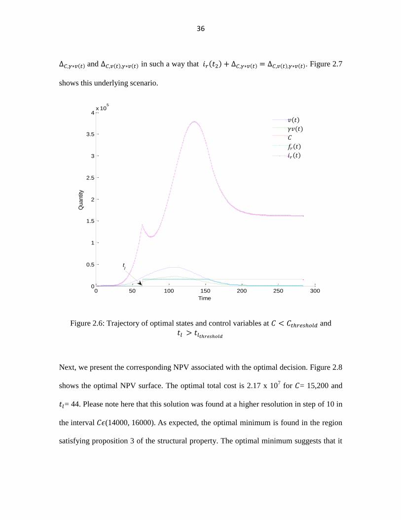
36
and in such a way that . Figure 2.7
shows this underlying scenario.
Figure 2.6: Trajectory of optimal states and control variables at and
Next, we present the corresponding NPV associated with the optimal decision. Figure 2.8
shows the optimal NPV surface. The optimal total cost is 2.17 x 10⁷ for = 15,200 and
= 44. Please note here that this solution was found at a higher resolution in step of 10 in
the interval (14000, 16000). As expected, the optimal minimum is found in the region
satisfying proposition 3 of the structural property. The optimal minimum suggests that it
0 50 100 150 200 250 3000
0.5
1
1.5
2
2.5
3
3.5
4x 10
5
Qu
an
tity
Time
v(t)
gam*v(t)
C
fr(t)
ir(t)
tl
37
is judicious decision is to delay the launch of remanufactured parts while satisfying
. By delaying the launch, a strategic level of recoverable core inventory is
built and thus needs of virgin parts are reduced after launch of remanufacturing program.
Whereas, installing corresponding capacity level at reduces otherwise high
virgin serviceable parts inventory level needed after end-of the production cycle.
Figure 2.7: Trajectory of optimal states and control variables at and
0 50 100 150 200 250 3000
0.5
1
1.5
2
2.5x 10
5
Time
Qu
an
tity
v(t)
gam*v(t)
C
fr(t)
ir(t)
tl
38
Figure 2.8: The structure of the optimal NPV
According to proposition 4, when , since capacity is less than the
that means manufacturing of more virgin parts, non-zero recoverable core
inventory at , and also virgin parts inventory will be held for longer period because is
shifted to the right. From cost perspective, although cost is saved by installing less
capacity, but it doesn‟t compensate for increase in cost due to total manufacturing cost,
total recoverable inventory holding cost and total serviceable inventory holding cost as
compared to case in proposition 3. For case, when , all costs is increased
as in case , including more recoverable inventory at because .
0
20
40
60
80
100
0.01
0.015
0.02
0.025
0
0.05
0.1
0.15
0.2
0.25
0.3
0.35
0.310.3
0.28
0.290.28
0.27
0.27
0.26
0.26
tl
0.25
0.25
0.24
0.250.26
0.240.23
0.23
0.22
0.27
0.24
0.23
0.250.240.23
0.220.22
0.23
C x 106
NP
V x
10
7
39
For proposition 5, we have two options, one suggests remanufacturing all recoverable
cores and other advocates it is optimal to produce less. In the first sub-case, in
comparison to proposition 3, cost is incurred due to increase in total capacity cost and
also pre-launch recoverable inventory holding cost. For second sub-case, cost is incurred
as described for proposition 4. Arguably cost incurred due to surplus recoverable
inventory could have been reduced if we had considered disposal activity in our model.
On the contrary, costs still have increased for all the cases as compared to proposition 3
due to inclusion of disposal cost of surplus cores. It should be noted here that in the
preceding analysis we kept all the parameters at nominal level otherwise it is trade-off
between core holding cost vs. virgin part inventory cost vs. capacity installation cost. We
will investigate this in next sub-section.
2.4.2 Effect of Parameters on Optimal Time to Launch and Optimal Capacity
In this section we will present the effect of each parameter- on ,
and %Rel.Savings. %Rel.Savings is calculated as follows:
(23)
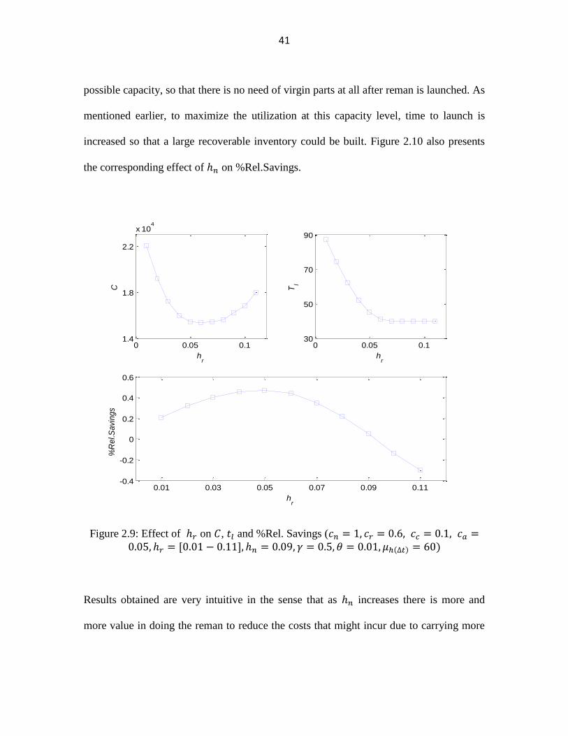
Figure 2.9 presents the effect of on optimal capacity, optimal time to launch and
%Rel.Savings. We observe that for lower values of , firm tends to install more capacity
and time to launch is also delayed. We believe this is because of two reasons. First, at
lower values of , it is cheaper to hold larger recoverable inventory for longer period
and then to capitalize on the high level of held inventory a larger capacity is installed.
Secondly, after the end of the production, recoverable inventory substitutes for
40
serviceable inventory. Therefore, at lower values firm tries to minimize the needs for
serviceable inventory after end of the production. Whereas, in case of higher values of
, as expected, time to launch shortens but surprisingly capacity increases. This can be
attributed to fact that at higher values firm doesn‟t differentiate much between
recoverable and serviceable inventory because cost associated is almost similar. Thus, it
tries to reduce cost that might be incurred due to holding large recoverable inventory
which can be done by launching earlier and installing more capacity so as to increase
differences in equilibrium of areas. Figures also reveal an interesting qualitative result.
The %Rel.Savings, first increases and reaches a peak and then decreases. For a small
value of , when it is optimal to carry a large recoverable inventory and capacity is less
likely to be constrained, the %Rel.Savings is low due to high capacity cost. Whereas, for
higher values, when there is not much of difference between recoverable and serviceable
inventory, still due to increase in capacity cost %Rel.Savings decrease. It is also
important to note here that when , it is not optimal to remanufacture as
%Rel.Savings becomes non-positive. This certifies our initial assumption regarding
remanufacturing that for remanufacturing to be profitable should be less than .
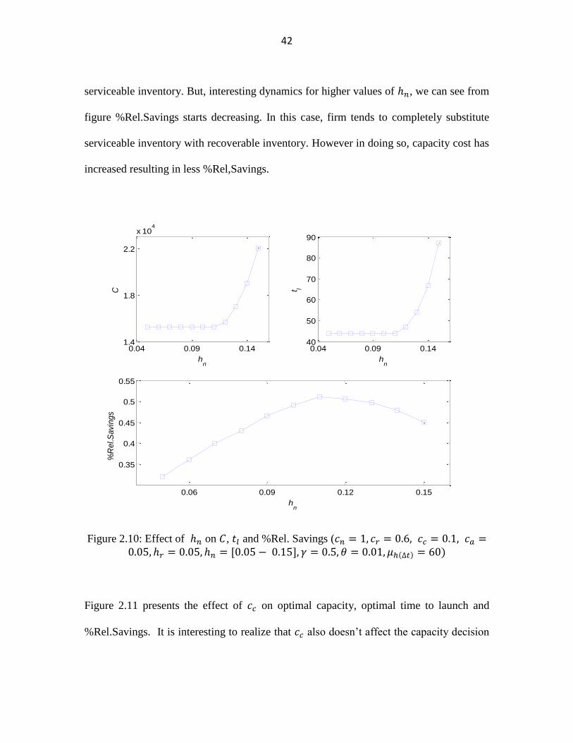
Effect of on optimal capacity, optimal time to launch and %Rel.Savings is
presented in Figure 2.10. It can seen from the figure that doesn‟t much affect the
decision related to time to launch and capacity except at very high value as compared to
. We believe for lower values, firm tries to maintain the equilibrium of areas. By doing
so, it reduces two important costs which are incurred due to manufacturing and carrying
serviceable inventory for longer duration. Whereas, for higher values, it picks maximum
41
possible capacity, so that there is no need of virgin parts at all after reman is launched. As
mentioned earlier, to maximize the utilization at this capacity level, time to launch is
increased so that a large recoverable inventory could be built. Figure 2.10 also presents
the corresponding effect of on %Rel.Savings.
Figure 2.9: Effect of on , and %Rel. Savings (
Results obtained are very intuitive in the sense that as increases there is more and
more value in doing the reman to reduce the costs that might incur due to carrying more
0 0.05 0.11.4
1.8
2.2
x 104
hr
C
0 0.05 0.130
50
70
90
hr
Tl
0.01 0.03 0.05 0.07 0.09 0.11-0.4
-0.2
0
0.2
0.4
0.6
hr
%R
el.S
avi
ng
s
42
serviceable inventory. But, interesting dynamics for higher values of , we can see from
figure %Rel.Savings starts decreasing. In this case, firm tends to completely substitute
serviceable inventory with recoverable inventory. However in doing so, capacity cost has
increased resulting in less %Rel,Savings.
Figure 2.10: Effect of on , and %Rel. Savings (
Figure 2.11 presents the effect of on optimal capacity, optimal time to launch and
%Rel.Savings. It is interesting to realize that also doesn‟t affect the capacity decision
0.04 0.09 0.141.4
1.8
2.2
x 104
hn
C
0.04 0.09 0.1440
50
60
70
80
90
hn
t l
0.06 0.09 0.12 0.15
0.35
0.4
0.45
0.5
0.55
hn
%R
el.S
avi
ng
s
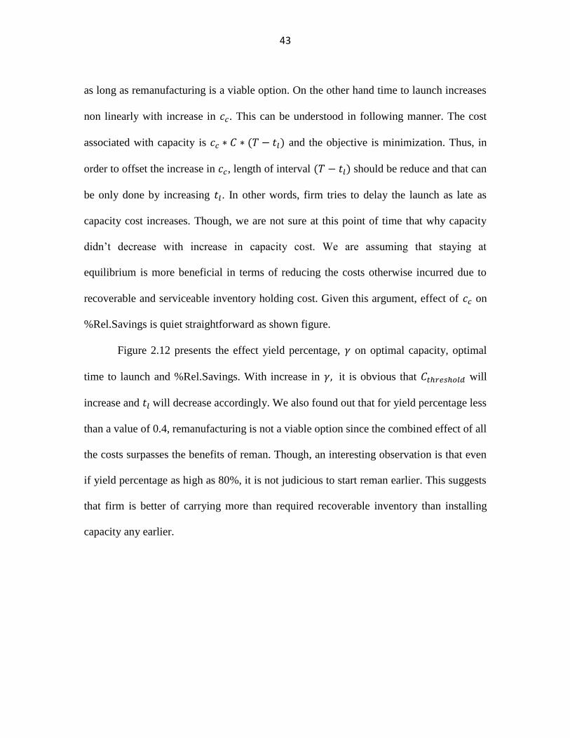
43
as long as remanufacturing is a viable option. On the other hand time to launch increases
non linearly with increase in . This can be understood in following manner. The cost
associated with capacity is and the objective is minimization. Thus, in
order to offset the increase in , length of interval should be reduce and that can
be only done by increasing . In other words, firm tries to delay the launch as late as
capacity cost increases. Though, we are not sure at this point of time that why capacity
didn‟t decrease with increase in capacity cost. We are assuming that staying at
equilibrium is more beneficial in terms of reducing the costs otherwise incurred due to
recoverable and serviceable inventory holding cost. Given this argument, effect of on
%Rel.Savings is quiet straightforward as shown figure.
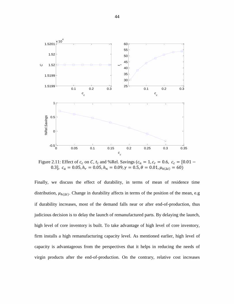
Figure 2.12 presents the effect yield percentage, on optimal capacity, optimal
time to launch and %Rel.Savings. With increase in it is obvious that will
increase and will decrease accordingly. We also found out that for yield percentage less
than a value of 0.4, remanufacturing is not a viable option since the combined effect of all
the costs surpasses the benefits of reman. Though, an interesting observation is that even
if yield percentage as high as 80%, it is not judicious to start reman earlier. This suggests
that firm is better of carrying more than required recoverable inventory than installing
capacity any earlier.
44
Figure 2.11: Effect of on , and %Rel. Savings (
Finally, we discuss the effect of durability, in terms of mean of residence time
distribution, . Change in durability affects in terms of the position of the mean, e.g
if durability increases, most of the demand falls near or after end-of-production, thus
judicious decision is to delay the launch of remanufactured parts. By delaying the launch,
high level of core inventory is built. To take advantage of high level of core inventory,
firm installs a high remanufacturing capacity level. As mentioned earlier, high level of
capacity is advantageous from the perspectives that it helps in reducing the needs of
virgin products after the end-of-production. On the contrary, relative cost increases
0.1 0.2 0.31.5199
1.5199
1.52
1.52
1.5201x 10
4
cc
C
0.1 0.2 0.325
30
35
40
45
50
55
60
cc
t l
0 0.05 0.1 0.15 0.2 0.25 0.3 0.35-0.5
0
0.5
1
cc
%R
el.S
avi
ng
s
45
because total core inventory holding cost as well as capacity installation cost has
increased. Thus, %Rel.Savings decreases.
Figure 2.12: Effect of on , and %Rel. Savings (
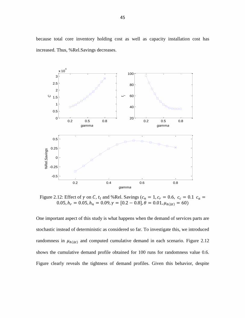
One important aspect of this study is what happens when the demand of services parts are
stochastic instead of deterministic as considered so far. To investigate this, we introduced
randomness in and computed cumulative demand in each scenario. Figure 2.12
shows the cumulative demand profile obtained for 100 runs for randomness value 0.6.
Figure clearly reveals the tightness of demand profiles. Given this behavior, despite
0.2 0.5 0.80
0.5
1
1.5
2
2.5
3
x 104
gamma
C
0.2 0.5 0.820
40
60
80
100
gammat l
0.2 0.4 0.6 0.8
-0.5
-0.25
0
0.25
0.5
gamma
%R
el.S
avi
ng
s
46
randomness, we suggest that deterministic study is very much valid and sufficient enough
to understand the underlying dynamics of capacity management.
Figure 2.13: Cumulative stochastic returns with randomness in mean of 0.6
2.5 Conclusion and Future Research
In this chapter, we presented the drivers of optimal strategic capacity management for
remanufactured products targeting aftermarket services. First, we analyzed properties of
dynamic situation with regard to product life cycle and returns to establish optimal reman
policy for aftermarket services. Then we presented an algorithm to compute optimal time
to launch and overall capacity requirement given various costs and life cycle parameters.
0 50 100 150 200 2500
0.5
1
1.5
2
2.5
3
3.5
4
4.5x 10
6
Time
Qu
an
tity
47
We also presented the structural properties of the optimal reman policy and demonstrate
how the optimal policy is a threshold policy in capacity and time to launch. Furthermore,
we compared our solution with no remanufacturing scenario and established when it is
optimal to reman.
Our analysis asserts that it is always optimal to delay the launch of
remanufacturing program in order to build a strategic recoverable inventory. This helps in
making the dynamics less supply constrained. But care should be taken in making such
decision since it is a trade-off between recoverable inventory holding cost and potential
relative savings. A high inventory holding cost decreases the profitability of
remanufacturing, especially if it is stocked for future remanufacturing. We also found out
that low cost of serviceable inventory of virgin parts doesn‟t affect decision regarding
time to launch. This is because, at low cost, when there is smaller deviation from
recoverable inventory holding cost, remanufactured units can imperfectly substitute the
virgin parts. Thus, decision largely depends on the cost of holding recoverable inventory.
But, at high cost of serviceable inventory, remanufactured units perfectly substitute virgin
parts and remanufacturing becomes attractable. Though, firm also needs to take into
account cost of capacity at high cost of serviceable inventory. For remanufacturing
capacity level, it is not optimal to install maximum possible capacity. A capacity level
should be selected such that it reduces the needs of serviceable inventory of virgin parts
after end of the OE production run. In this study, we couldn‟t figure out why cost of
capacity doesn‟t influence time to launch decision. Though, we presented a reasonable
argument, but a better study needs to be carried out and thus subject of future research.
48
A number of possibilities exist for further research in this area. Though, we have
shown that deterministic analysis is very powerful in realizing the important insights
regarding effective reman program, yet a complete stochastic analysis could be very
interesting and valuable. Further, we considered a single product environment; an
extension of this work focusing in multi-product environment by analyzing joint
distributions of the product returns are very much possible.
REFERENCES
Barros, A. I., Dekker, R., Scholten, V. 1998. A two-level network for recycling sand: a
case study. European Journal of Operational Research, 110, 199–214
Beullens, P. 2001. Location, process selection, and vehicle routing models for reverse
logistics. Ph.D. thesis, Centre for Industrial Management, KU Leuven, Belgium.
Chittamvanich, S., Ryan, S. M. 2004. Using forecasted information from early returns of
used products to set remanufacturing capacity. Working paper.
Debo , L. G., Toktay, L. B., Wassenhove, L. N. Van. 2006. Joint Life-Cycle Dynamics of
New and Remanufactured Products. Production and Operations Management. 15(4),
498–513
Ferrer, G., D. C. Whybark. 2001. Material planning for a remanufacturing facility.
Production and Operations Management. 10(2) 112–124.
Fleischmann, M. 2001. Quantitative Models for Reverse Logistics. Lecture Notes in
Economics and Mathematical Systems, Vol. 501. Springer, Berlin, Germany.
49
Francasa, D., Minner, Stefan. 2009, Manufacturing network configuration in supply
chains with product recovery. Omega, 37, 757-769
Franke, C., Basdere, B., Ciupek, M., Seliger, S., 2006. Remanufacturing of mobile
phones–capacity, program and facility adaptation planning. Omega. 34, 562–570.
Georgiadis, P., Athanasiou. 2010. The impact of two-product joint lifecycles on capacity
planning of remanufacturing networks. European Journal of Operational Research, 202
(2), 420-433
Georgiadis, P., Vlachos, D. 2004. The effect of environmental awareness on product
recovery networks design. European Journal of Operational Research, 157, 449–64.
Georgiadis, P., Vlachos, D., Tagaras, G., 2006. The impact of product lifecycle on
capacity planning of closed-loop supply chains with remanufacturing. Production &
Operations Management, 15, 514–527.
Geyer, R., L. N. Van Wassenhove, A. Atasu. 2006. The economics of remanufacturing
under limited component durability and finite life cycle, Management Science, 53(1), 88–
100
Guide, V. D. R., Jr., Harrison, T. P., L. Van Wassenhove. 2003. The Challenge of
Closed-Loop Supply Chains, Interfaces, 33(6) 3–6
Guide, V. D. R., Jr., M. E. Kraus, R. Srivastava. 1997. Scheduling policies for
remanufacturing. International Journal of Production Research. 48(2) 1081–1091.
50
Guide, V. D. R., Jr., V. Jayaraman, R. Srivastava, W. C. Benton. 1998. Supply chain
management for recoverable manufacturing systems. Interfaces, 30(3) 125–142.
Ilgin, M. A., Gupta, S. M. 2010. Environmentally conscious manufacturing and product
recovery (ECMPRO): A review of the state of the art. Journal of Environmental
Management, 91 563–591
Kleber, R. 2006.The integral decision on production/remanufacturing technology and
investment time in product recovery. OR Spectrum, 28, 21–51
Louwers, D., Kip, B. J., Peters, E., Souren, F., Flapper, S. D. P. 1999 A facility location
allocation model for reusing carpet materials. Computers and Industrial Engineering, 36,
855–869
Mutha, A., Pokharel, S., 2009. Strategic network design for reverse logistics and
remanufacturing using new and old product modules. Computers & Industrial
Engineering, 56, 334–346.
Realff, M. J., Ammons, J. C., Newton, D. J.2004, Robust reverse production system
design for carpet recycling. IIE Transactions, 36, 767–776.
Shih, L. 2001. Reverse logistics system planning for recycling electrical appliances and
computers in Taiwan. Resources, Conservation and Recycling, 32(1), 55-72.
Toktay, L. B., L. M. Wein, S. A. Zenios. 2000. Inventory management of
remanufacturable products. Management Science. 46(11) 1412–1426.
51
Van der Laan, E., M. Salomon, R. Dekker, L. Van Wassenhove. 1999. Inventory control
in hybrid systems with remanufacturing. Management Science. 45(5) 733–747.
Vlachos, D., Georgiadis, P., Iakovou, E. 2007. A system dynamics model for dynamic
capacity planning of remanufacturing in closed-loop supply chains. Computers
& Operations Research, 34, 367–394.
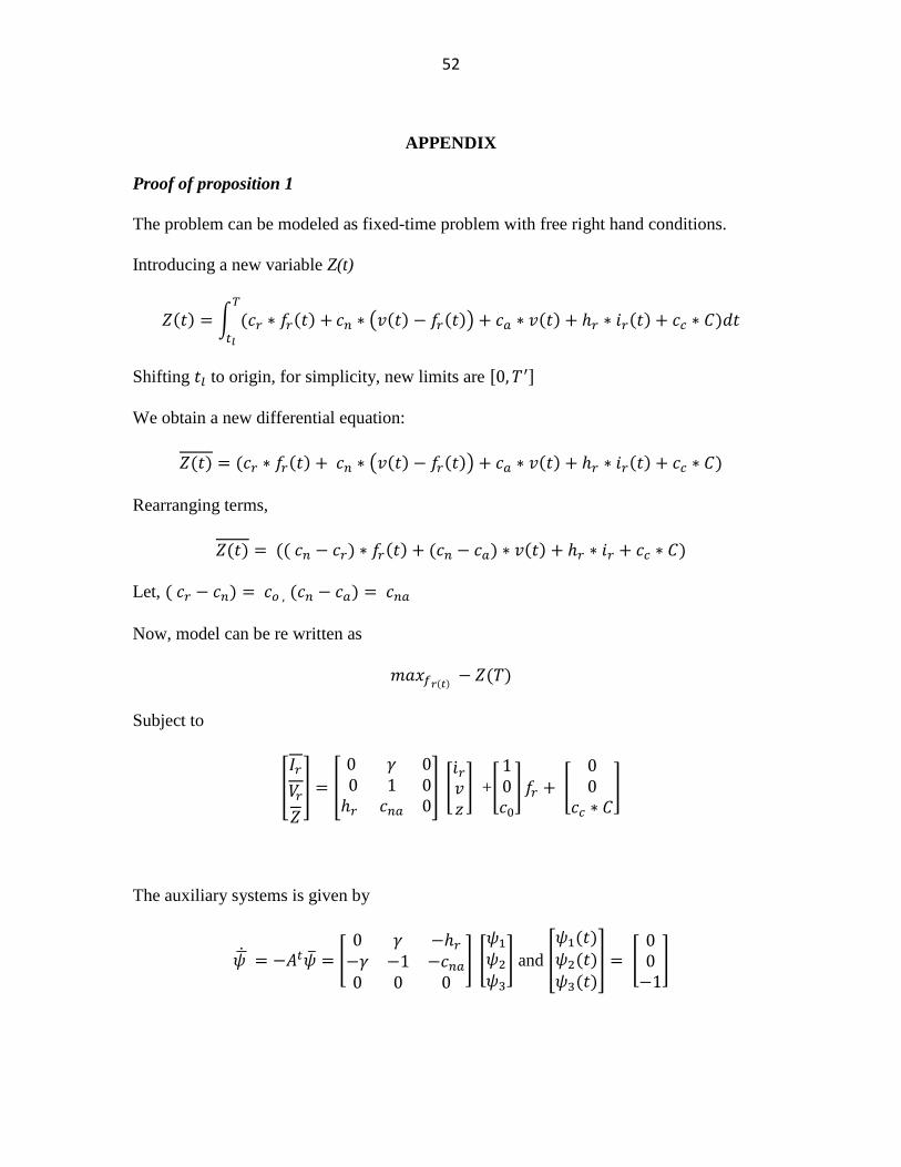
52
APPENDIX
Proof of proposition 1
The problem can be modeled as fixed-time problem with free right hand conditions.
Introducing a new variable Z(t)
Shifting to origin, for simplicity, new limits are
We obtain a new differential equation:
Rearranging terms,
Let,
Now, model can be re written as
Subject to
+
The auxiliary systems is given by
and
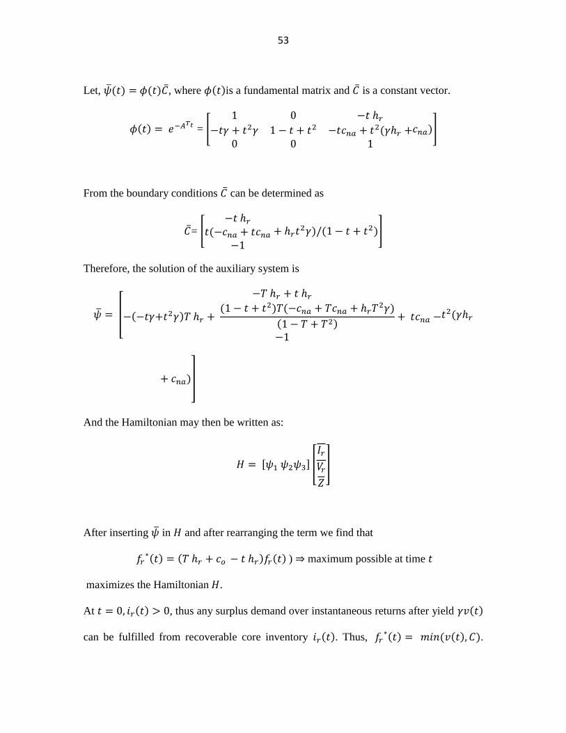
53
Let, , where is a fundamental matrix and is a constant vector.
=
From the boundary conditions can be determined as
=
Therefore, the solution of the auxiliary system is
And the Hamiltonian may then be written as:
After inserting in and after rearranging the term we find that
) maximum possible at time
maximizes the Hamiltonian .
At , thus any surplus demand over instantaneous returns after yield
can be fulfilled from recoverable core inventory . Thus, .
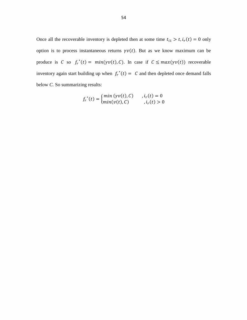
54
Once all the recoverable inventory is depleted then at some time only
option is to process instantaneous returns . But as we know maximum can be
produce is so . In case if recoverable
inventory again start building up when and then depleted once demand falls
below C. So summarizing results:
55
Chapter 3 : HAZARD RATE MODELS FOR CORE RETURNS FORECASTING IN
REMANUFACTURING
Efficient production planning is a very important lever of a profitable remanufacturing
program at operational level. A production planning system for remanufacturing assists
managers making decisions regarding disassembly, remanufacturing, manufacturing, and
coordinating between disassembly and reassembly. Among various factors which affect
the production planning, accurate estimation of core returns is an important input for an
efficient planning. Nevertheless, the uncertainty in the timing and quantity of returns
makes core returns forecasting a very challenging task in remanufacturing milieu.
As aforementioned in chapter 2, this research was also pursued on a request from
a tier-1 automotive supplier engaged in OE production and also providing aftermarket
services. Management was interested in improving the accuracy of their core forecasting
method because the existing forecast method was too simplistic to capture the dynamics
of core returns in the face of uncertainty in timing/location of return, return volume,
quality etc. The particular interest was in understanding the dynamics of independent
aftermarket (IAM) returns. IAM core returns is more challenging than original equipment
services or warranty claims because of increased uncertainty in the returns. Unlike the
OE service setting, the trade in process is often not initiated with the receipt of a core but
with an order. The setting is as follows. Supplier receives orders for reman parts from a
number of automotive aftermarket parts retailers/distributors (e.g., NAPA), OE service
and parts operations organizations (e.g., GM SPO), and large dealers, referred to here
upon as the “customer”. In shipping the order, the supplier imposes a “core charge” on
56
the customer, a debit that will be credited to the customer upon receiving the defective
part or the “core”. The supplier issues a return material authorization (RMA) in shipping
the order, to facilitate return shipment of cores. Efficient production and inventory
management of reman parts for the supplier heavily impinges on the ability to accurately
forecast these core returns from customers (besides forecasting demand for reman parts
and securing cores from the open market, as necessary). There are several challenges to
this, including, the volume and diversity of customers, differences among individual
customer warehouses in returning cores, large reman product catalog, changing customer
behaviors (often improving core return delays), and data sparsity.
In this chapter, we have reported the evidence for the effectiveness of hazard rate
regression models to calculate return delay distribution in the context of remanufacturing.
We extensively studied various types of hazard rate modelling technique (e.g.,
parametric, semi-parametric etc.) and its appropriateness. Further, we described various
approaches when underlying proportionality assumptions is violated or when there is
time-varying effect of covariates or there is randomness in one of the covariates. To the
best of our knowledge, no existing literature has explored all these issues in context of
returns modelling for remanufacturing.
Rest of the chapter is organized as follows: Related literature is presented in section 3.2.
Proposed framework is discussed in section 3.3. A real world case study is presented in
Section 3.4. Results and discussion have been presented in section 3.5. Finally,
conclusion and future research in section 3.6.
57
3.2 Literature Review
Over the last two decades, there has been significant research in the area of
remanufacturing and reverse logistics. Guide (2000) carried out an extensive survey of
reman literature and identified future research needs. Based on existing literature, he
divided reman research into five broad categories: forecasting, reverse logistics,
production planning and control, inventory control and management, and general.
Further, he identified seven complicating characteristics that complicate the production
planning and control activities of reman industry: 1) the uncertain timing and quantity of
returns, 2) the need to balance returns with demands, 3) the disassembly of returned
products, 4) the uncertainty in materials recovered from returned items, 5) the
requirement for a reverse logistics network, 6) the complication of material matching
restrictions, and 7) the problems of stochastic routings for materials for remanufacturing
operations and highly variable processing times. In recent years, the last four
complication categories have been addressed extensively ( Aras (2008), Barba-Gutierrez
(2008), Inderfurth (2004), Krikke (2008), Li (2009), Takahashi (2007), Tang (2005),
Wang (2007)). Since, our research focus here will be on the first complicating
characteristic; forecasting, we encourage readers to refer a recent survey by Ilgin and
Gupta (2010) for research in the other categories.
Toktay et al. (2000) presented the role of forecasting in managing product returns
and argued how predicting returns influences decision at strategic, tactical, and
operational levels. They also quoted that there are only few documented business
examples dealing with forecasting in reverse logistics. Ilgin and Gupta (2010), reiterate
58
this statement by citing only eight notable publications. However, most of these
publications assume that the core return probability is known in advance (e.g., Goh &
Varaprasad (1986), Kelle and Silver (1989))
Most of the extant literature exploited the fact that future returns are a function of
past sales. Goh & Varaprasad (1986) are credited for being the first to develop such a
model. They propose a transfer function model to estimate return quantities of Coca-Cola
bottles in Malaysia and Singapore markets using Box-Jenkin‟s time-series techniques to
compute life-cycle parameters. Kelle and Silver (1989) proposed four forecasting
techniques based on available information sets to estimate the “net demand” during lead
time of reusable containers. As noted earlier these models assumed that returns are
Poisson with known rate. To overcome this limitation, Toktay et al. (2000) considered a
queuing network based approach to achieve an optimal ordering policy for Kodak‟s
single use-camera. The model utilized a Bayesian estimation and expectation
optimization approach to forecast returns in a trackable as well as untrackable case.
Although, their method doesn‟t require known return rate but makes assumption
regarding the shape of lag distribution.
Aforementioned methods used past sales and return data to forecast returns. Hess
and Mayhew (1997) employed split adjusted hazard model and time regression to model
merchandise return in direct marketing. They incorporated explanatory variables in their
regression. Marx-G´omez et al. (2002) develop a fuzzy inference system for the
forecasting of returns. Their model included demand, life cycle parameters, and return
incentives with the fuzzy rule-base developed from prior expert knowledge.
59
The extant literature offers a few returns forecasting models but these models are
simply not practical for many suppliers, such as our collaborator Delphi Product &
Service Solutions, a sub-division of Delphi Corporation that provides replacement parts
and services to the automotive aftermarket, because:
1. Virtually all these models are applicable for forecasting returns of
individual products/SKUs
2. The historical data is simply too sparse to facilitate modelling and
calibration of models for individual SKUs.
3. Makes one or other assumption based on expert/prior knowledge (e.g.,
return rate is known or shape of lag model is known).
Thus, it becomes imperative to build effective and efficient models for forecasting core
returns in the automotive IAM, from the perspective of a Tier-1 automotive parts
supplier.
One of the most interesting characteristics of returns data is right-censoring,
which means at any given time only a fraction of returns is observed whereas rest of them
are outstanding, and thus requires analysis of duration time. Typically, an analyst tends to
achieve three modeling objectives while investigating duration time data (Helsen and
Schmittlen 1993): effects of covariate, dynamics of duration, and duration time
forecasting. They also listed short-comings in conventional modeling approaches
(duration time regression, logit, probit etc.) as follows:
1. Use of duration time regression in the face of censoring may lead to biased
estimates of the covariate effects;
60
2. Time regression and logit/probit models are inappropriate when there are time
varying covariates; and
3. In case of probit/logit models, for predictions, time intervals should be integer
multiples of censoring times.
Literature suggests (Gupta 1991, Jain and Vilcassim 1991, Helsen and Schmittlen 1993)
that hazard rate regression models can overcome the above listed shortcomings while
achieving all three objectives within a single tractable class of duration time models.
Further, Helsen and Schmittlen (1993) established that hazard rate regression models
outperform conventional procedures (e.g. duration time regression, logit, probit etc.) in
terms of stability of the estimates, face validity of parameter estimates, and predictive
accuracy.
3.3 The Modelling Framework
As stated earlier, core returns can be modeled using duration time modeling within a
single tractable class of hazard rate models. This section provides a brief overview of
hazard rate models.
Let denote the hazard rate at time t for an individual having covariate
values at time t. Thus, the covariate values may vary over time for
any individual. This hazard rate is assumed to take the form
(1)
Where indicates the effect of covariate on the hazard rate, and is the baseline
hazard function. Thus the model has two multiplicative components. The first, ,
61
captures the longitudinal regularities in duration time dynamics. The second, ,
adjusts up or down proportionately to reflect the effect of the measured covariates.
In light of this proportional adjustment of the baseline hazard rate, estimation of the -
vector in (1) is termed proportional hazards regression (PHR).
In most applications is formulated as an exponential function:
(2)
Which renders the estimation of easier, given that no constraints need to be imposed to
ensure non-negativity of .
3.3.1 Semi Parametric Modelling (Cox-proportional Hazard rate model)
Cox proportional hazard model is one of the most widely used tools in survival analysis.
It gained a lot attention of researches since its development in 1972 due to its efficiency
and flexibility. This could be attributed to semi-parametric nature of the model which
doesn‟t make any special assumption regarding the distribution of failure occurrence also
know as baseline hazard function. Cox‟s major contribution was to suggest an estimation
technique- partial likelihood to purely estimate regression coefficients , allowing for a
general hazard function as nuisance parameter. He also suggested that this can result in
slight loss of information about . Efron (1977) and Oakes (1977) provide evidence
indicating that maximizing the partial likelihood results in very efficient estimates of .
Tsiatis (1981) shows that under general conditions the partial MLE is consistent and
asymptotically normal.
62
For duration time processes, the usual ("total") likelihood has as the event of
interest the fact that individuals s duration time (i.e., the random variable took on the
observed value for individuals The partial likelihood also focuses
on the observed durations , but considers them in a different way. Imagine that
individual i has an uncensored duration . At this duration time , a number of
other individuals were "at risk," i.e., had not yet experienced the duration event (the "risk
set"). Of all those at risk, individual , is the one who actually experienced the duration at
, and it is this selection event that the partial likelihood considers. Thus, the partial
likelihood is the likelihood that individual is the one, of those at risk, who has the
duration of , given that someone is known to have a duration of .
Since the hazard rate measures the likelihood of the duration event
happening at for those who have made it up to time without experiencing an event,
this rate deter-mines the odds of selection in the partial likelihood for each individual at
risk. Thus, for an observed time at which individual experiences a duration ( ),
the partial likelihood that this duration indeed happened to individual (and not to one of
the other individuals at risk) is
(3)
Where is the number of individuals at risk at , and these individuals are denoted
. Substituting the proportional hazards model (2) in (3) yields
(4)
for which the longitudinal effect cancels, leaving
63
(5)
The partial likelihood estimate of is obtained by maximizing the product of
expression (4) over all observed duration times. Note that, unlike the usual duration time
regression models, the right-censored observations do enter the partial likelihood (5), i.e.,
these individuals, each having some covariate vector were at risk at but did not
experience the duration. The information in this event relevant for the response
coefficient is appropriately taken into account in (4). To summarize, the only thing
"partial" about the partial likelihood is in the event it chooses to model. The total
likelihood is concerned with the total duration event, i.e., "When will the duration occur
for each individual?" The partial likelihood considers only part of the total duration
event, namely, "Given that a duration occurred to someone at a specific time, which
individual, of those still at risk, experienced it?" Since the answer to this latter question
hinges on the relative riskiness of various individuals all measured at the same duration
time, it comes as no surprise that the longitudinal effects drop out in (3), leaving
(4) dependent only on the desired response coefficients 1.
Cox-model has gained popularity because it works well in practice. Practitioner
believes that in process of considering possible models, Cox model should always
considered as an option. This is attributable to the flexibility of the model which only
requires proportional hazard assumption. It has also been established that Cox model is
reasonably robust to modest departure from proportional hazard. Further, in many cases
variables can be transformed to show approximate proportional hazard (discusses in
section 5.3).
64
3.3.2 Parametric Modeling
Parametric models assume that base-line hazard function; follows known
functional form, e.g.: Exponential, exponential, logistics etc. Computationally, biggest
advantage of parametric model is, one can use full maximum likelihood to estimate the
parameters. This in turn provides meaningful estimate of effects. Parametric models are
better choice if modeller has better knowledge of the aging process. In literature,
researchers always caution the use of parametric model since most of the time prior
knowledge is not always available. But, this does not rule out the option of comparing
parametric models against semi-parametric models.
3.4 Case Study
To establish the empirical performance of the proposed framework, we tested it on IAM
return data of an engine control module (ECM). Electronic Control Modules are
subsystems consisting of CPUs and assorted signal inputs and outputs dedicated to
controlling a component within the vehicle. They range in complexity from an Engine
Control Unit which handles the logic for managing the power-train system efficiency, to
an Anti-lock Braking (ABS) Control unit that monitors vehicle speed and brake fluid, to a
simple body module that controls the automatic door locks or power windows (National
Instruments).
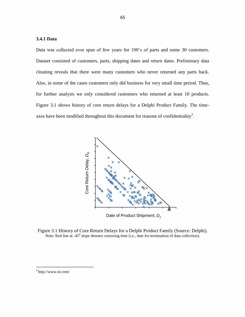
65
3.4.1 Data
Data was collected over span of few years for 100‟s of parts and some 30 customers.
Dataset consisted of customers, parts, shipping dates and return dates. Preliminary data
cleaning reveals that there were many customers who never returned any parts back.
Also, in some of the cases customers only did business for very small time period. Thus,
for further analysis we only considered customers who returned at least 10 products.
Figure 3.1 shows history of core return delays for a Delphi Product Family. The time-
axes have been modified throughout this document for reasons of confidentiality3.
Figure 3.1 History of Core Return Delays for a Delphi Product Family (Source: Delphi). Note: Red line at -45
0 slope denotes censoring time (i.e., date for termination of data collection).
3 http://www.ni.com/
0
100
200
300
400
500
600
700
800
900
1000
0 200 400 600 800 1000 1200Date of Product Shipment, Ds
Co
reR
etu
rn D
ela
y, D
R
66
3.4.2 Nomenclature
This section provides necessary nomenclature to facilitate duration modelling in an IAM
setting. In this case, we have used right censoring for truncation.
DA: Census Date
DS: Shipment Date
DR: Day product was returned (if it is returned)
R: If product is returned it is 1 else 0
T: It is defined as time since DS until DR or DA, depending on returned or not
Pi: Products, i=1, 2, 3 …
Ci: Customers, i=1, 2, 3 …
Now, we can construct a hazard rate model with set of covariates X = [P, C], and
dependent variable T with censoring R. Mathematically,
(6)
3. 5. Results and Discussion4
In this section we present results of the numerical case study. First we discuss the
estimates of the covariates for parametric and semi-parametric hazard rate models. Then,
we show the validity of the underlying models in the face of stability, efficiency and
4 All these experimentation were done using Survival package in Software R (http://cran.r-project.org/). For
time-by-covariate interactions, we used COXPHF package
(http://www.meduniwien.ac.at/msi/biometrie/programme/fc/)
67
predictive performance. Finally, we discuss how to pursue modelling using extended Cox
ph models when proportionality assumption is violated.
3.5.1 Parameter Estimates
To assess the suitability of parametric modelling, we chose widely known parametric
proportional hazard model-Weibull; whereas, Cox proportional hazard rate model for
semi-parametric modelling. First requirement was to ensure the effect of covariates.
Our initial analysis revealed that none of the products were statistically significant from
each other. Thus, we assumed that all products are identical and chose customers as only
covariate for the modelling. Table 3.1 summarizes the results obtained. Results indicated
that both model have monotonically increasing hazard rate. Monotonically increasing
hazard rates seems highly intuitive since we are modelling return- likelihood of return of
a product increases with elapsed time. Statistically, both models are very significant with
p-values at 0. Also, individual estimates for each customers obtained are highly
significant. Further, the sign of coefficients explains the returning behaviour of a
customer- positive value depicts that customer makes faster returns and vice-versa.
Expected return behaviour of customers is shown in figure 3.2. It was surprising to
realize, in case of most of the customer, that instead of returning core back after receiving
a shipment from supplier immediately; customer tends to delay it infinitely. A possible
reason seems to be that rather than trade-in, customer wants to stock the parts to handle
stock-out situation. Other reasons could be a core-collector is buying it at high price than
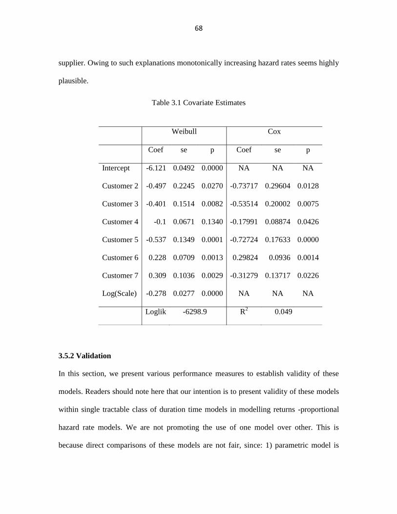
68
supplier. Owing to such explanations monotonically increasing hazard rates seems highly
plausible.
Table 3.1 Covariate Estimates
Weibull Cox
Coef se p Coef se p
Intercept -6.121 0.0492 0.0000 NA NA NA
Customer 2 -0.497 0.2245 0.0270 -0.73717 0.29604 0.0128
Customer 3 -0.401 0.1514 0.0082 -0.53514 0.20002 0.0075
Customer 4 -0.1 0.0671 0.1340 -0.17991 0.08874 0.0426
Customer 5 -0.537 0.1349 0.0001 -0.72724 0.17633 0.0000
Customer 6 0.228 0.0709 0.0013 0.29824 0.0936 0.0014
Customer 7 0.309 0.1036 0.0029 -0.31279 0.13717 0.0226
Log(Scale) -0.278 0.0277 0.0000 NA NA NA
Loglik -6298.9 R2 0.049
3.5.2 Validation
In this section, we present various performance measures to establish validity of these
models. Readers should note here that our intention is to present validity of these models
within single tractable class of duration time models in modelling returns -proportional
hazard rate models. We are not promoting the use of one model over other. This is
because direct comparisons of these models are not fair, since: 1) parametric model is
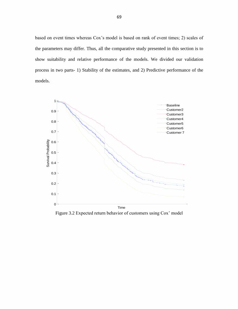
69
based on event times whereas Cox‟s model is based on rank of event times; 2) scales of
the parameters may differ. Thus, all the comparative study presented in this section is to
show suitability and relative performance of the models. We divided our validation
process in two parts- 1) Stability of the estimates, and 2) Predictive performance of the
models.
Figure 3.2 Expected return behavior of customers using Cox‟ model
0
0.1
0.2
0.3
0.4
0.5
0.6
0.7
0.8
0.9
1
Time
Su
rviv
al P
rob
ab
ility
Baseline
Customer2
Customer3
Customer4
Customer5
Customer6
Customer 7
70
3.5.2.1 Stability and Efficiency of the Estimates
To check the stability of the estimates, we referred to methods proposed by Krsitiaan and
Helsen (1993). In their work, they considered two samples from different market as
calibration and validation dataset. Since, in our case we do not have two different dataset
thus, we considered these samples: 1) Complete-dataset (I), 2) 50% of complete dataset
as Calibration-dataset (II), and 3) rest of the 50% as Validation-dataset (III). One should
note here that taking a totally random sample may compromise uniformity, since we have
returns as well as non-returns. So, in order to retain uniformity across samples, we
considered 50% of returns and 50% of non-returns for each calibration and validation
samples. We re-estimated all the models for calibration and validation dataset. To
evaluate the relative efficiency of the estimates, we evaluated standardized measures of
variability, SV (= σβ/|β|), for all the models on all the samples. SV is analogous to the
coefficient of variations, where cases with parameter estimates close to zero are
emphasized (Nardi and Schemper, 2003).
Table 3.2 presents the estimated coefficients and SV’s (in parentheses) for each
sample for both models. Table 3.2 shows incredible performance of the models in term of
stability of the parameter estimates. There is remarkable consistency (ignoring minor
discrepancies) between calibration and validation dataset (Only notable discrepancy in
case of customer 2 where departure is as high as 10% for both the models). More
interestingly, there is very small departure from estimates obtained from complete dataset
versus calibration and validation dataset (mostly less that 5%). Also, there is no change in
the sign of coefficients. This dictates the suitability of proportional hazard rate models for
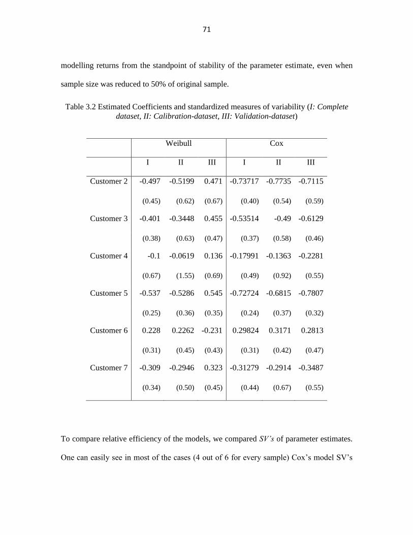
71
modelling returns from the standpoint of stability of the parameter estimate, even when
sample size was reduced to 50% of original sample.
Table 3.2 Estimated Coefficients and standardized measures of variability (I: Complete
dataset, II: Calibration-dataset, III: Validation-dataset)
Weibull Cox
I II III I II III
Customer 2 -0.497 -0.5199 0.471 -0.73717 -0.7735 -0.7115
(0.45) (0.62) (0.67) (0.40) (0.54) (0.59)
Customer 3 -0.401 -0.3448 0.455 -0.53514 -0.49 -0.6129
(0.38) (0.63) (0.47) (0.37) (0.58) (0.46)
Customer 4 -0.1 -0.0619 0.136 -0.17991 -0.1363 -0.2281
(0.67) (1.55) (0.69) (0.49) (0.92) (0.55)
Customer 5 -0.537 -0.5286 0.545 -0.72724 -0.6815 -0.7807
(0.25) (0.36) (0.35) (0.24) (0.37) (0.32)
Customer 6 0.228 0.2262 -0.231 0.29824 0.3171 0.2813
(0.31) (0.45) (0.43) (0.31) (0.42) (0.47)
Customer 7 -0.309 -0.2946 0.323 -0.31279 -0.2914 -0.3487
(0.34) (0.50) (0.45) (0.44) (0.67) (0.55)
To compare relative efficiency of the models, we compared SV’s of parameter estimates.
One can easily see in most of the cases (4 out of 6 for every sample) Cox‟s model SV‟s

72
were closer to zero as contrast to Weibull model. Thus, in relative sense we can conclude
that Cox‟s model performed better than Weibull based on standard measures of
variability.
3.5.2.2 Predictive Performance of the Models
We compared different model‟s prediction with observed returns. In order to facilitate
these comparisons we considered two performance measures: hit rates (Krsitiaan and
Helsen, 1993) and mean square errors (MSE) in forecast.
Hit rates can be defined as percentage of returns correctly classified. To calculate
hit rates, we require hazard rate model forecasts for median duration and observed return
for median duration. Hazard rate model forecasts for median duration implies,
computation of time point at which the survival function drops below 0.5 and then
interpolating linearly to produce forecast for median duration. Table 3.3 presents hit
rates for both models for all the samples. For Cox‟s model hit rates are as high as 90%.
Cox‟s model performed remarkably well as compared to Weibull model. This difference
can be better understood by analyzing survival plot for base-line for both the models
(Figure 3.3). One can easily see that Cox‟s model tries to fit to the data better due its
flexibility as compared to Weibull with rigid structure.
Next, we considered mean square error in forecast. To achieve this objective, Data set is
divided into 5 time period. The same procedure, as used to predict forecast for mean
duration, can be used to generate forecasts for each time-periods. In this scenario, we will
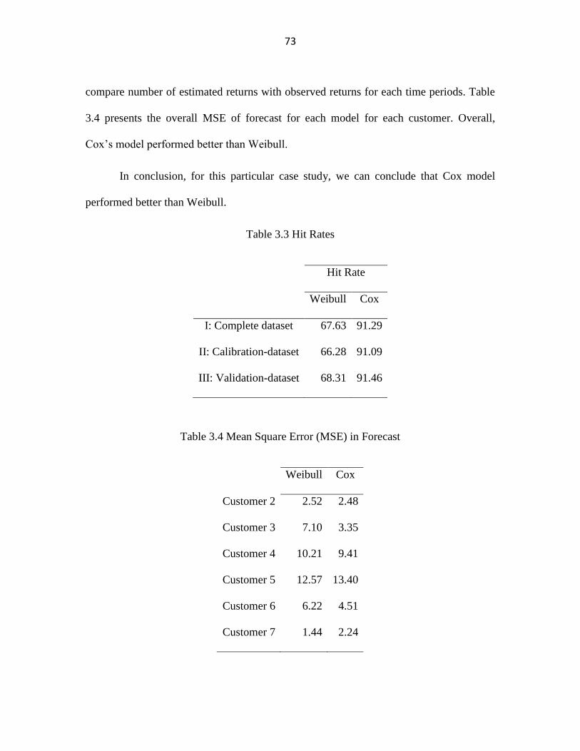
73
compare number of estimated returns with observed returns for each time periods. Table
3.4 presents the overall MSE of forecast for each model for each customer. Overall,
Cox‟s model performed better than Weibull.
In conclusion, for this particular case study, we can conclude that Cox model
performed better than Weibull.
Table 3.3 Hit Rates
Hit Rate
Weibull Cox
I: Complete dataset 67.63 91.29
II: Calibration-dataset 66.28 91.09
III: Validation-dataset 68.31 91.46
Table 3.4 Mean Square Error (MSE) in Forecast
Weibull Cox
Customer 2 2.52 2.48
Customer 3 7.10 3.35
Customer 4 10.21 9.41
Customer 5 12.57 13.40
Customer 6 6.22 4.51
Customer 7 1.44 2.24
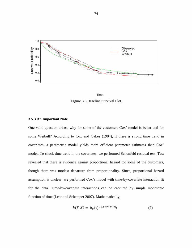
74
Figure 3.3 Baseline Survival Plot
3.5.3 An Important Note
One valid question arises, why for some of the customers Cox‟ model is better and for
some Weibull? According to Cox and Oakes (1984), if there is strong time trend in
covariates, a parametric model yields more efficient parameter estimates than Cox‟
model. To check time trend in the covariates, we performed Schonfeld residual test. Test
revealed that there is evidence against proportional hazard for some of the customers,
though there was modest departure from proportionality. Since, proportional hazard
assumption is unclear; we performed Cox‟s model with time-by-covariate interaction fit
for the data. Time-by-covariate interactions can be captured by simple monotonic
function of time (Lehr and Schemper 2007). Mathematically,
(7)
0.0
0.2
0.4
0.6
0.8
1.0
Time
Surv
ival P
robab
ility
Observed Cox Weibull
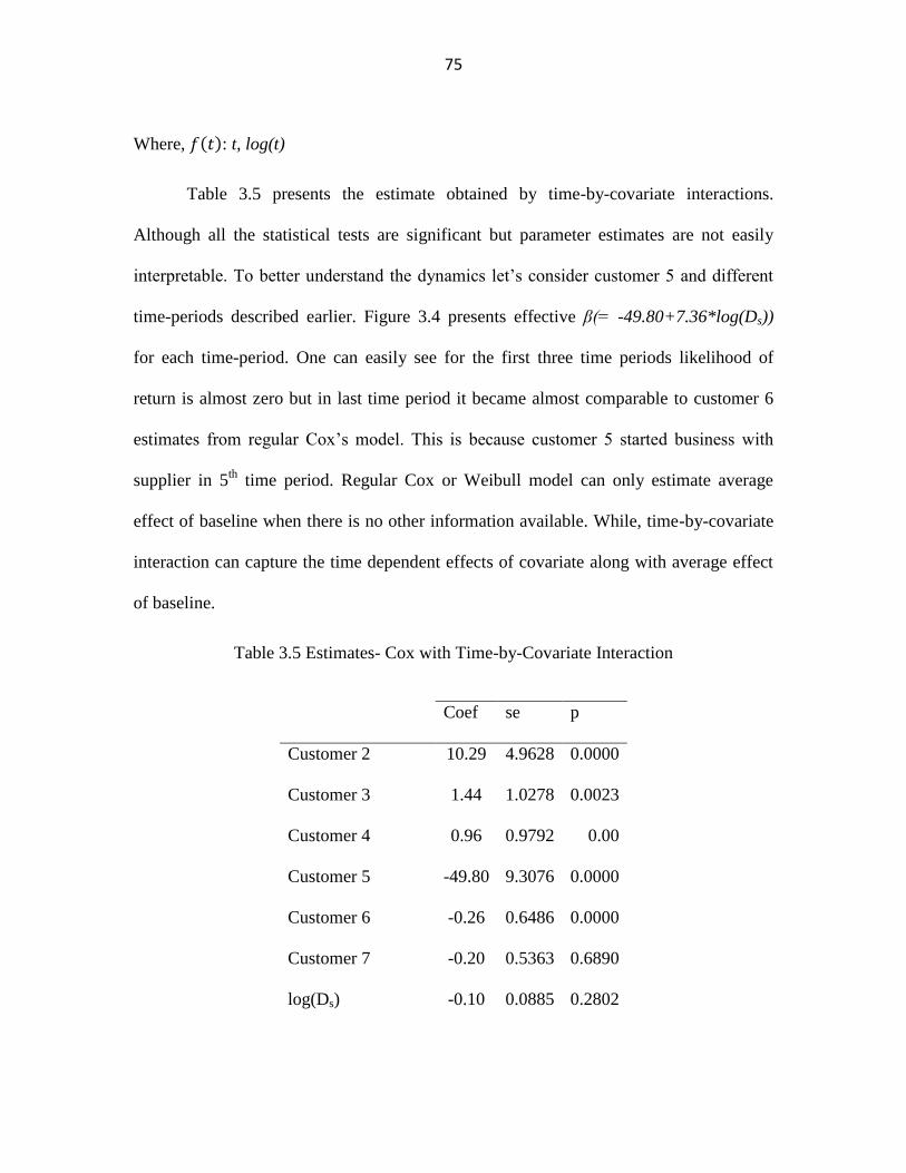
75
Where, : t, log(t)
Table 3.5 presents the estimate obtained by time-by-covariate interactions.
Although all the statistical tests are significant but parameter estimates are not easily
interpretable. To better understand the dynamics let‟s consider customer 5 and different
time-periods described earlier. Figure 3.4 presents effective β(= -49.80+7.36*log(Ds))
for each time-period. One can easily see for the first three time periods likelihood of
return is almost zero but in last time period it became almost comparable to customer 6
estimates from regular Cox‟s model. This is because customer 5 started business with
supplier in 5th
time period. Regular Cox or Weibull model can only estimate average
effect of baseline when there is no other information available. While, time-by-covariate
interaction can capture the time dependent effects of covariate along with average effect
of baseline.
Table 3.5 Estimates- Cox with Time-by-Covariate Interaction
Coef se p
Customer 2 10.29 4.9628 0.0000
Customer 3 1.44 1.0278 0.0023
Customer 4 0.96 0.9792 0.00
Customer 5 -49.80 9.3076 0.0000
Customer 6 -0.26 0.6486 0.0000
Customer 7 -0.20 0.5363 0.6890
log(Ds) -0.10 0.0885 0.2802
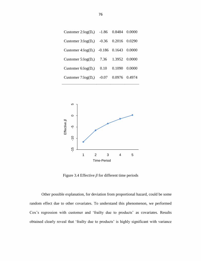
76
Customer 2:log(Ds) -1.86 0.8484 0.0000
Customer 3:log(Ds) -0.36 0.2016 0.0290
Customer 4:log(Ds) -0.186 0.1643 0.0000
Customer 5:log(Ds) 7.36 1.3952 0.0000
Customer 6:log(Ds) 0.10 0.1090 0.0000
Customer 7:log(Ds) -0.07 0.0976 0.4974
Figure 3.4 Effective β for different time periods
Other possible explanation, for deviation from proportional hazard, could be some
random effect due to other covariates. To understand this phenomenon, we performed
Cox‟s regression with customer and „frailty due to products‟ as covariates. Results
obtained clearly reveal that „frailty due to products‟ is highly significant with variance
-15
-10
-50
5
1 2 3 4 5
Eff
ective β
Time-Period
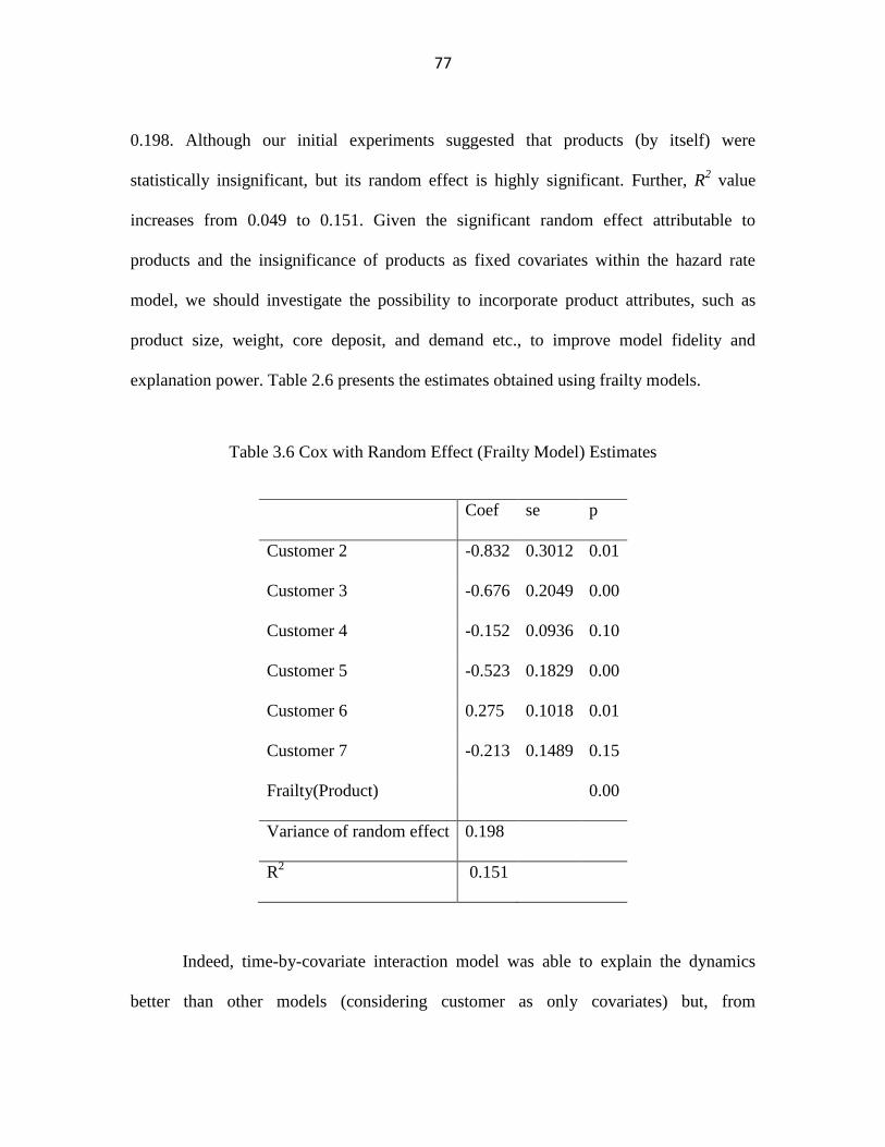
77
0.198. Although our initial experiments suggested that products (by itself) were
statistically insignificant, but its random effect is highly significant. Further, R2 value
increases from 0.049 to 0.151. Given the significant random effect attributable to
products and the insignificance of products as fixed covariates within the hazard rate
model, we should investigate the possibility to incorporate product attributes, such as
product size, weight, core deposit, and demand etc., to improve model fidelity and
explanation power. Table 2.6 presents the estimates obtained using frailty models.
Table 3.6 Cox with Random Effect (Frailty Model) Estimates
Coef se p
Customer 2 -0.832 0.3012 0.01
Customer 3 -0.676 0.2049 0.00
Customer 4 -0.152 0.0936 0.10
Customer 5 -0.523 0.1829 0.00
Customer 6 0.275 0.1018 0.01
Customer 7 -0.213 0.1489 0.15
Frailty(Product) 0.00
Variance of random effect 0.198
R2 0.151
Indeed, time-by-covariate interaction model was able to explain the dynamics
better than other models (considering customer as only covariates) but, from
78
computational complexity point of view other models were far more superior. This is
because, with time-by-covariate interactions, there will be a baseline hazard rate for every
time stamp. Thus, choosing one of these models is trade-off between computational
complexity and degree of accuracy one is intend to achieve. In our case, Cox‟s model
performed satisfactory (ignoring modest departure from proportionality) to meet the
requirements.
3.6. Conclusions and Future Work
This research presents a unified approach for modeling returns in an automotive
independent aftermarket setting. It helped in understanding the customer behaviour,
which tends to be attracted by the open-market deals or try to stock the products instead
of trading. Results are also beneficial when suppliers are planning to kick-off new reman
product in the market. Further, based on our insights, products attribute can bring more
robust and promising results than just considering products by itself.
A range of hazard rate models has been presented to facilitate returns modelling.
This research does not try to advocate one type of models over other since it depends on
experts/analysts discretion what he is trying to achieve. For our analysis, we found Cox‟s
model sufficient enough to meet our requirements. We reiterate the flexibility and ease of
use of Cox‟ model were outstanding. Although, we modeled a particular setting but
presented model is capable of achieving higher level of scalability and can easily be
replicated in any industry.
79
REFERENCES
Aksen, D., Aras, N., Karaarslan, A.G., 2009. Design and analysis of government
subsidized collection systems for incentive-dependent returns. International Journal of
Production Economics 119, 308–327.
Aras, N., Aksen, D., 2008. Locating collection centers for distance- and incentive
dependent returns. International Journal of Production Economics 111, 316–333.
Barba-Gutierrez, Y., Adenso-Diaz, B., Gupta, S.M., 2008. Lot sizing in reverse MRP for
scheduling disassembly. International Journal of Production Economics 111, 741–751.
Box, G. E. P., G. M. Jenkins. 1976. Time Series Analysis, Forecasting and Control,
revised edition, Holden-Day, San Francisco.
Cox, D. R., and Oakes, D. 1984. Analysis of Survival Data, Chapman and Hall.
Goh, T. N., and Varaprasad, N. 1986. A statistical methodology for the analysis of the
life-cycle of reusable containers. IIE Transactions 18, 42-47.
Guide, V.D.R., 2000. Technical Note: Production planning and control for re
manufacturing: industry practice and research needs. Journal of Operations Management
18, 467–483.
Gupta, S., (1991), Stochastic Models of Interpurchase Time with Time-Dependent
Covariates, Journal of Marketing Research, 28, 1-15.
80
Helsen, K., and Schmittlen, D. C., 1993. Analyzing Duration Times in Marketing:
Evidence for the Effectiveness of Hazard Rate Models, Marketing Science, 12 (4), 395-
414.
Hess, J. D., and Mayhew, G. E. 1997. Modeling merchandise returns in direct marketing.
Journal of Direct Marketing 11 (2), 20-35.
Ilgin, M. A., and Gupta, S. M., 2010. Environmentally conscious manufacturing and
product recovery (ECMPRO): A review of the state of the art, Journal of Environmental
Management, 91, 563–591.
Inderfurth, K., 2004. Optimal policies in hybrid manufacturing/remanufacturing systems
with product substitution. International Journal of Production Economics 90, 325–343.
Jain, D. C. and N. Vilcassim, 1991. "Investigating Household Purchase Timing
Decisions: A Conditional Hazard Function Approach," Marketing Science, 10, 1-23.
Kelle, P., and Silver, E. A., 1989. Forecasting the returns of reusable containers. Journal
of Operations Management 8 (1), 17-35.
Krikke, H., le Blanc, I., van Krieken, M., Fleuren, H., 2008. Low-frequency collection of
materials disassembled from end-of-life vehicles: on the value of on-line monitoring in
optimizing route planning. International Journal of Production Economics 111, 209–228.
Li, J., Gonzalez, M., Zhu, Y., 2009. A hybrid simulation optimization method for
production planning of dedicated remanufacturing. International Journal of Production
Economics 117, 286–301.
81
Marx-Gómez, J., Rautenstrauch, C., and Nürnberger, A. 2002. Neuro-fuzzy approach to
forecast returns of scrapped products to recycling and remanufacturing. Knowledge-
based Systems 15, 119-128.
Nardi, A., and Schemper, M., 2003. Comparing Cox and parametric models in clinical
studies, Statistics In Medicine, 22, 3597–3610
Oakes, D., 1977. The asymptotic information in censored survival data. Biometrika,
64:441–448.
Stephan Lehr and Michael Schemper. 2007. Parsimonious analysis of time-dependent
effects in the Cox model. Statistics In Medicine, 26, 2686–2698
Takahashi, K., Morikawa, K., MyreshkaTakeda, D., Mizuno, A., 2007. Inventory control
for a MARKOVIAN remanufacturing system with stochastic decomposition process.
International Journal of Production Economics 108, 416–425.
Tang, O., Grubbstro¨m, R.W., 2005. Considering stochastic lead times in a
manufacturing/ remanufacturing system with deterministic demands and returns.
International Journal of Production Economics 93, 285–300.
Toktay, B., Wein, L., and Zenios, S. 2000. Inventory management of remanufacturable
products. Management Science 46 (11), 1412-1426.
Wang, Z., Yao, D.Q., Huang, P., 2007. A new location-inventory policy with reverse
logistics applied to B2C e-markets of China. International Journal of Production
Economics 107, 350–363.
82
Chapter 4 : CONCLUSION AND FUTURE RESEARCH
Over the last few decades, OEMs and suppliers have realized that there are tremendous
opportunities to engage in remanufacturing business to improve profitability and
sustainability. However, efficient management of remanufacturing program is known for
its complexity. This is mostly attributed to limited visibility in reverse logistics systems.
Our collaboration with one of the tier 1 supplier indicated that there is lack of a structured
and holistic decision support framework, which can guide firms in decision making
related to timing the launch of the remanufacturing program, capacity
installation/management etc. Further, efficient production and inventory management of
remanufacturing parts for the supplier heavily impinges on the ability to accurately
forecast these core returns from customers (besides forecasting demand for
remanufacturing parts and securing cores from the open market, as necessary). Based on
request from our collaborator and existing gaps in related literature survey, this research
has proposed an integrated decision support framework for remanufacturing in
aftermarket services. Though, focus of this thesis is mainly on automotive aftermarket
services but models introduced are robust enough to fit in most of the remanufacturing
environment.
In this research, we have tackled two interrelated problems of reman program at
strategic and operational level. At strategic level, we have studied the capacity
management in launch of reman program for aftermarket services. This objective requires
making decision on optimal time to launch of the reman program and overall capacity
83
requirement. The pre-requisite of this objective is to first compute an optimal reman
policy given a time to launch and capacity level. To pursue this, we have analytically
derived optimal reman policy by minimizing total cost associated with reman. Our
analysis revealed that in the presence of supply and capacity constraint, the optimal
reman policy is a threshold policy in time to launch and capacity. This suggests that if
time to launch and capacity is not in the range of their respective threshold values, it is
not possible to reman all returns. Thus, total cost associated with reman program will be
higher since firm couldn‟t exploit the option of remanufacturing all collected returns.
Given optimal policy, it becomes evident that there exist an optimal time to launch and
optimal capacity level for a reman program. To compute optimal time to launch and
capacity level, we proposed a heuristics solution method to minimize the discounted cash
outflow given an optimal reman policy. We found out that it is always in the best interest
of the firm to delay the launch of a reman program to build a strategic recoverable
inventory. Regarding capacity, most of the existing literature assumes that there is
enough capacity level available for remanufacturing. On the contrary, our analysis
suggests that it is not always optimal to install maximum capacity level. Working at
maximum capacity level is only beneficial if reman program commences after end of the
regular production. In that case, a high level of strategic inventory is built thus reman is
not supply constrained. Further, we extensively studied the drivers of cost-effective
remanufacturing in terms of various cost, product and life cycle parameters. Following
are the specific contributions of our study at strategic level:
84
(i) This is the first study that systematically accounted and explicitly modeled reman
policy, time to launch and capacity level within a single modeling framework.
Most of the prior research focused on evaluating these decisions disjointedly.
(ii) We exploited the fact that each return generates demand for an aftermarket
service parts due to trade-in process. Thus, demand for aftermarket service parts
is same as core returns.
(iii) An optimal reman policy is obtained analytically using pontygrain maximum
principle.
(iv) A heuristics solution algorithm is formulated to obtain the time to launch and
capacity. Previous study in computation of time to launch did not account for
optimal capacity level (Kleber, 2006). They assumed that there is sufficient
capacity to reman most of the returns.
(v) We have analytically derived the structural properties of optimal reman policy in
presence of both supply and capacity constraints.
(vi) A closed-form expression for threshold value of time to launch and capacity is
accomplished in this study.
(vii) Sensitivity analysis revealed many managerial insights important in achieving
cost-effective reman program.
(viii) Finally, our analysis of stochastic returns revealed that underlying deterministic
analysis is very robust and efficient in capturing most important drivers of
remanufacturing for aftermarket services.
85
At operational level, we studied the core-returns forecasting in remanufacturing. Most of
the extant literature dealing with returns forecasting typically assumed that probability
distribution of returns is already known. Furthermore, models were simply not practical
for many suppliers, such as our collaborator, because the historical return data was
simply too sparse to facilitate modelling and calibration of models for individual SKUs.
Additionally, there were several challenges to this, including, the volume and diversity of
customers, differences among individual customer warehouses, large remanufacturing
product catalogue, and changing customer behaviours (often improving core return
delays with time). To overcome these complications, we proposed an integrated
modelling framework that relies on products and customers among others as covariates
for forecasting returns among product families within a single tractable class of duration
modelling.
In this thesis, we have reported the evidence for the effectiveness of hazard rate
regression models to calculate return delay distribution in the context of remanufacturing.
We extensively studied various types of hazard rate modelling technique (e.g.,
parametric, semi-parametric etc.) and its appropriateness. Further, we described various
approaches when underlying proportionality assumptions is violated or when there is
time-varying effect of covariates or there is randomness in one of the covariates. To the
best of our knowledge, no existing literature has explored all these issues in context of
returns modelling for remanufacturing. Furthermore, we also provided valuable insights
based on our analysis regarding customer behaviour and made necessary
86
recommendation for firms in aftermarket remanufacturing business. Following are the
specific contributions of our study at operational level:
(i) We studied the effectiveness of hazard rate models in context of automotive
remanufacturing targeted for independent aftermarket.
(ii) Parametric, semi-parametric and extended Cox proportional models have been
exploited in modeling core returns within a single tractable class of duration time
modeling.
(iii) For our analysis, we realized semi-parametric, Cox proportional hazard rate
model, is powerful enough to understand the dynamics of IAM.
(iv) Results obtained from extended Cox proportional hazard rate model revealed two
important characteristics:
a. There is a time-varying effect of covariate and thus a time-by-covariate
interaction is more appropriate approach to model IAM data. However,
we showed that time-by-covariate interaction is very complicated
modeling technique, thus selection models should be based on the trade-
off between accuracy vs. complexity.
b. There is randomness due to covariate which is captured by
implementation of covariates model.
(v) Based on our analysis, we made following recommendations:
87
a. Instead of trading in core, customer tends to stock the product to handle
any stock-out situation.
b. Customer is attracted the open-market deals on cores. Thus, firm needs to
build a better incentive mechanism which can encourage customer to
return the cores.
c. Frailty model suggested that there is randomness in the process because
of the product. Thus, there is opportunity of incorporating product
attributes, such as product size, weight, core deposit, and demand etc., to
improve model fidelity and explanation power.
4.1 Future Research
The undertaken research is a very first step in building integrated decision support
framework for remanufacturing while catering needs to real world problem. Here, we
briefly discuss a few potential areas that are worth exploring:
(i) Our research study was focus on development of new facilities for a single
remanufactured product. Since, product development and production and
introduction are continuous process, it is important to incorporate the product
portfolio instead of a single product analysis. Our research can be used as a
starting point for such studies.
(ii) We focused on making one time decision regarding capacity and assumed with
time elapsed the investment can be considered as a sunk cost. But, typically,
capacity management considers capacity expansion and contraction based on
88
market response. Thus, it is worth exploring dynamic capacity management in
context of remanufacturing program.
(iii) We considered the OES and IAM jointly with 100% service level. Generally,
100% service level constraint is not very valid assumption. Thus, explicit
modeling of IAM could be more insightful in considering remanufacturing
program for IAM. More explicit model should be able to answer questions such
as; should firm launch remanufacturing program for independent aftermarket,
should firm operate at full capacity or capacity contraction is more attractive etc.
(iv) One important cost which undertaken research completely ignored is the cost of
disposal. We believe that there is some value in incorporating disposal cost in the
model. However, to account disposal, more sophisticated modeling is required.
(v) In order to increase the explaining power and fidelity of the models for core-
forecasting, product attributes can play a significant role.
(vi) A new avenue for research in aftermarket services can be development of better
incentive mechanism to encourage customer for quick returns.
89
ABSTRACT
AN INTEGRATED DECISION SUPPORT FRAMEWORK FOR
REMANUFACTURING IN THE AUTOMOTIVE INDUSTRY
by
AKHILESH KUMAR
August 2011
Advisor: Dr. Ratna Babu Chinnam
Major: Industrial Engineering
Degree: Doctor of Philosophy
In today‟s global economy, firms are seeking any and every opportunity to differentiate
from competitors by reducing supply chain costs and adding value to end customers. One
increasingly popular option, under growing consumer awareness and increasing
legislation, is to reintegrate returned products into the supply chain to achieve economic
benefits as well as improve sustainability. An important class of such “reverse” goods
flows has to do with remanufacturing (reman), which refers to activities that restore
returned products (“cores”) or their major modules to operational condition for using in
place of new product or distributing through other channels (e.g., spare parts). While
opportunities abound, some key complications reported in the literature include: 1)
difficulty in timing the launch of reman product (while accounting for uncertainties
associated with product life-cycle demand and core supply), 2) difficulty with capacity
planning for remanufacturing (while accounting for the fact that volumes can be low and
that facilities/lines should target multiple product families for economies of scale), and 3)
90
operational difficulties in maintaining efficiencies in production planning and control of
remanufacturing activities. These difficulties are mostly attributable to limited visibility
and higher levels of uncertainty in reverse logistics (in comparison with forward
logistics). Despite advances in the remanufacturing literature in the last two decades
(both in the academic literature and practitioner community), there is no integrated
decision support framework that can guide companies to successful launch and execution
of remanufacturing operations. This is particularly true for companies that engage in both
original equipment (OE) service as well as the independent after-market (IAM) in the
automotive industry. This research aims to address these limitations by developing a
decision support framework and necessary models for effective remanufacturing in the
automotive industry.
At the strategic level, we propose a unified approach to explicitly model and
address issues of capacities as well timing the launch of remanufacturing programs for
new product. We derive the optimal remanufacturing policy and extensively studied the
drivers of cost-effective remanufacturing program for aftermarket services. Our policies
exploit the ability to leverage OE production to support both the OE service operations as
well as demand from the IAM. To the best of our knowledge, this research is the first
attempt of its kind in the remanufacturing literature, as prior research treated these
interrelated decisions separately. Valuable managerial insights are obtained by
minimizing the discounted cash outflows caused by appropriate investment and core
return inventory building decisions. We show that, under certain conditions, it may be
optimal to delay the launch of the remanufacturing program to build up an adequate
91
initial core return inventory. This may help in perfectly substituting virgin parts with
remanufactured parts after end of the OE production run.
At operational level, efficient production planning and control of reman parts for
the supplier heavily impinges on the ability to accurately forecast core returns from
customers (e.g., dealers, distributors). There are several challenges to this, including, the
volume and diversity of customers served by the supplier, differences among individual
customer warehouses in returning cores, large reman product catalogs, changing
customer behaviors (often improving core return delays), and data sparsity. In this
research we report the evidence for the effectiveness of hazard rate regression models to
estimate core return delays in the context of remanufacturing. We investigate a number of
hazard rate modelling techniques (e.g., parametric, semi-parametric etc.) using real-world
datasets from a leading Tier-1 automotive supplier. Results indicate the effectiveness of
the proposed framework in terms of stability and face validity of the estimates and in
predictive accuracy.
92
AUTOBIOGRAPHICAL STATEMENT
NAME: AKHILESH KUMAR
EDUCATION
Ph. D: Industrial Engineering, Wayne State University, USA, 2011
B.Tech: Manufacturing Engineering, National Institute of Foundry and Forge
Technology, India, 2005
PUBLICATIONS
“Timing the Launch of Reman Program and Optimal Capacity to Install in An
Automotive Aftermarket Setting” to be submitted to Production and Operations
Management (Ready for Submission)
“Framework for Core Returns Forecasting of Auto Parts Remanufacturing” to be
submitted to International Journal of Production Economics (Ready for
Submission)
“Hidden-Markov Model based Sequential Clustering for Autonomous Diagnostics
and Prognostics” to be submitted to IEEE Transactions on Automation Science
and Engineering (Ready for Submission)
Kumar, A , Prakash, Tiwari, M.K., Shankar, R. and Baveja, A., (2006) “Solving
Machine Loading Problem of a Flexible Manufacturing System with Constraint
Based Genetic Algorithm” European Journal of Operational Research, pp
175(2), 1043-1069
Kumar, A., Prakash, A., Shankar, R., and Tiwari, M.K.; (2006), “Psycho-Clonal
algorithm based approach to solve continuous flow shop scheduling
problem”, Expert Systems with Applications, 31, pp. 504–514
Tiwari, M.K., Prakash, Kumar, A., and Mileham, A. R., (2005), “Determination
of Optimal Assembly Sequence Using Psycho Clonal Algorithm”, IMechE, Part-
B, Journal of Engineering Manufacture, Vol 219, pp 137-149
CONFERENCE PROCEEDINGS
Kumar, A., Tseng, F., and Chinnam, R. B., “Role of Hidden-Markov Models for
Autonomous Diagnostics” Proc. of IEEE International Symposium on
INnovations in Intelligent SysTems and Applications ( INISTA), Istanbul,
Turkey, June 15-18, 2011
Kumar, A., Tseng, F., Guo, Y., and Chinnam, R. B., “Hidden-Markov Model
Based Sequential Clustering for Autonomous Diagnostics,” Proc. of IEEE
International Joint Conference on Neural Networks (IJCNN), Hong Kong, June
1-6, 2008
Anand, R. B., Kumar, A., Tiwari, M. K., and Verma, K. K., „Optimization of
Electrical Discharge Machining Process using Taguchi‟s Quality Loss Function
and Fuzzy Rule Based System‟, Presented at National Workshop on Six Sigma
Implementation in Foundry/Forge Industries at NIFFT Ranchi, April, 2004