NASA / TM-2003-212297 IECEC-2002-20095

An Integrated Magnetic Circuit Model and Finite Element Model Approach to Magnetic Bearing Design

Andrew J. Provenza Glenn Research Center, Cleveland, Ohio

Andrew Kenny and Alan B. Palazzolo Texas A&M University, College Station, Texas

Prepared for the 37th Intersociety Energy Conversion Engineering Conference sponsored by the Institute of Electrical and Electronics Engineers, Electron Devices Society Washington, DC, July 28-August 2,2002

National Aeronautics and Space Administration

Glenn Research Center

April 2003

https://ntrs.nasa.gov/search.jsp?R=20030056642 2018-06-26T06:17:46+00:00Z

W

AN INTEGRATED MAGNETIC CIRCUIT MODEL AND FINITE ELEMENT MODEL APPROACH TO MAGNETIC BEARING DESIGN

Andrew J. Provenza National Aeronautics and Space Administration

Glenn Research Center Cleveland, OH 44135

Andrew Kenny Alan 6. Palauolo Texas A8M University

Department of Mechanical Engineering Vibration Control and Electromechanics Laboratory

College Station, TX 77843

ABSTRACT

A code for designing magnetic bearings is described. The code generates curves from magnetic circuit equations relating important bearing performance parameters. Bearing parameters selected from the curves by a designer to meet the requirements of a particular application are input directly by the code into a three-dimensional finite element analysis preprocessor. This means that a three-dimensional computer model of the bearing being developed is immediately available for viewing. The finite element model solution can be used to show areas of magnetic saturation and make more accurate predictions of the bearing load capacity, current stiffness, position stiffness, and inductance than the magnetic circuit equations did at the start of the design process. In summary the code combines one-dimensional and three-dimensional modeling methods for designing magnetic bearings.

INTRODUCTION

Magnetic bearings must meet certain specifications such as size, load capacity, frequency response bandwidth, and other parameters. This paper describes a design code used to automate the calculation of these parameters. Advances toward more accurate prediction of the bearing parameters have been made by others such as Schweitzer (1994), Hawkins (1997), and Palauolo et al. (2001). Usually these advances focused on improvements to one dimensional magnetic circuit calculations or to multidimensional finite element analysis. The method described herein takes advantage of these advances by combining one dimensional magnetic circuit calculations with three dimensional finite element calculations in an integrated manner.

In this approach the one-dimensional magnetic circuit equations are arranged to generate plots showing the relationships between all the parameters.

NASAiTM-2003-2 12297

The designer uses these plots to pick the best combination of performance parameters that meet the requirements of the particular application. This choice of parameters necessarily fixes the dimensions of the bearing, which are sent to a finite element analysis preprocessor, and a three-dimensional model is created, analyzed, and the results are available for comparison to the one-dimensional circuit model predictions.

MAGN ETlC Cl RCU IT APPROACH

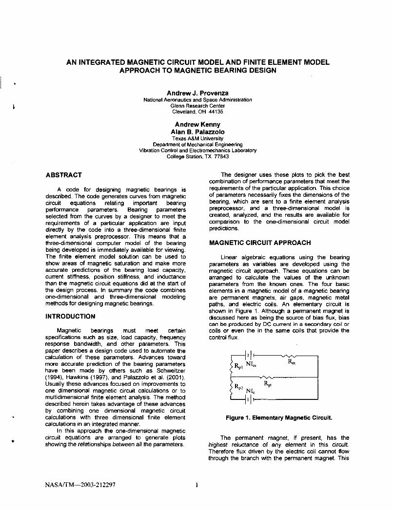
Linear algebraic equations using the bearing parameters as variables are developed using the magnetic circuit approach. These equations can be arranged to calculate the values of the unknown parameters from the known ones. The four basic elements in a magnetic model of a magnetic bearing are permanent magnets, air gaps, magnetic metal paths, and electric coils. An elementary circuit is shown in Figure 1. Although a permanent magnet is discussed here as being the source of bias flux, bias can be produced by DC current in a secondary coil or coils or even the in the same coils that provide the control flux.

Figure 1. Elementary Magnetic Circuit.

The permanent magnet, if present, has the highest reluctance of any element in this circuit. Therefore flux driven by the electric coil cannot flow through the branch with the permanent magnet. This

1

fact is often used to simplify the magnetic circuit models of magnetic bearings by breaking the multi- loop circuits into simpler single loop circuits for the permanent magnet flux and the electric coil flux as by Lee, Hsiao, and KO, (1994).

The total air gap reluctance, R,, , which includes

at least two separate physical air gaps, has the next highest reluctance after the permanent magnet in Figure 1. Although the permanent magnet and the air gap have nearly the same permeability, the permanent magnet is much longer than the air gap, which must be very thin to allow flux driven through it by the electric coils with out excessive current.

The ferromagnetic paths have a very low reluctance. The important exception is in the direction perpendicular to laminates in a stack.

Equations 1 to 2 are the equations for the magnetomotive force produced by the electric coil, NZ,, and permanent magnet, NI, . In these

equations, N is the number of turns in the coil, 1, is

the current in the coil, H,is the magnet coercivity,

and I , is the magnet length.

NI, = H , * 1, Eq. 1

NZc = N , * I , Eq. 2

The circuit path reluctances depend on their cross section areas, lengths, and material permeabilities and are given by Equations 3 to 5.

Here R , is the reluctance of the magnet, R,, is the

reluctance of the air gap, and R, is the reluctance of

the metal path. The cross section area and length are given by, A and 1 , and the permeability is indicated by l u .

Eq. 3

Eq. 4 4 P o A,

R, =-

RI, =- 4 Eq. 5 Po A ,

Kirchoff's laws are used to calculate the magnetic flux flowing through the loops. The two loop equations for Figure 1 are given by equations 6 and 7. The flux through the permanent magnet loop is the bias flux, q, , and the flux through the control loop is & . These

equations can be rearranged to solve for any of the geometric and magnetic variables. This illustrates the key advantage of the circuit model approach.

Eq. 7

The circuit model approach's main limitation is the inaccuracy of the simple circuits used to model. In fact, in one specific compact homopolar radial bearing design for a flywheel energy storage application, nearly fifty percent of the flux produced by the permanent magnet does not circulate through the magnet circuit, but bypasses the circuit through the air adjacent to the magnet. This leakage effect has to be estimated and used to reduce the value of bias flux used in subsequent calculations after it is calculated from Equation 6. Another effect that must be estimated is called air gap fringing. It is dilution of the flux density in the air gap by flux escaping out the air gap sides. This effect must also be estimated and is typically found by multiplying the bias and control flux densities calculated from Equations 6 and 7 by a fudge factor.

The error from these estimates is amplified in calculations of the position stiffness and current stiffness, which are proportional to the bias flux.

Geometric constraint equations can be combined with the electromagnetic circuit equations to calculate dimensions for various types of bearing configurations such as heteropolar, homopolar, and TAMU bias pole as discussed by Kenny, Provenza and Palazzolo et. al. (2001). The magnetic path dimensions are sized to allow room for all the coil turns required to drive sufficient flux. The path cross-sectional areas must be balanced to prevent magnetic saturation in all path branches. Other bearing dimensions can be limited by the size of the machine in which the bearing is placed. The rotor outer diameter can be limited by the stresses due to high-speed rotation.

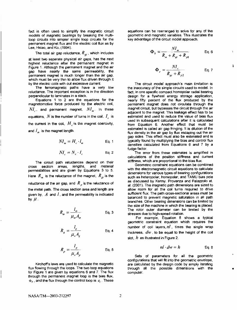
For example, Equation 8 shows a typical geometric constraint equation which requires the number of coil layers, nl , times the single wrap thickness, dw , to be equal to the height of the coil slot, h as illustrated in Figure 2.

nl - dw = h Eq. 8

Sets of parameters for all the geometric configurations that will fit into the geometric envelope, are calculated by the design code by simply iterating through all the possible dimensions with the computer.

I

NASAITM-2003-2 12297 2

magnet 0-- - -

coil layers

Figure 2. Simplified Graphical Representation of a Magnetic Bearing Circuit Showing Geometric

Constraint of Coil Wire Slots.

THREE DIMENSIONAL FINITE ELEMENT METHOD APPROACH

Three dimensional finite element methods are well established for electromagnetic analysis. Several textbooks have been written on the subject, including those by Salon (1995) and Ida & Bastos (1997). Several commercial codes complete with preprocessors for modeling geometry, magnetostatic and time varying solvers, and post processors are available. In this work, Opera 3D by Vector Fields was used.

Traditionally the drawback of finite element analysis has been the time required to build a model. The advent of solid model preprocessors in the early nineties helped somewhat, as did automatic mesh generators. However a slow manual input was required every time a new magnetic bearing design needed to be analyzed. This reduced the finite element analysis to mainly a check of designs determined from the equations derived by one- dimensional circuit analysis.

Recently solid model preprocessors have been introduced with parametric capability. Dimensions, material properties, electric current levels, and other parameters of the magnetic bearing can be specified as variable parameters. Essentially each type of magnetic bearing, (heteropolar, homopolar, or bias pole), only needs to be manually input into the preprocessor once. After that new configurations of the same type of bearing can be analyzed simply by changing the values of the parameterized dimensions. This significantly enhances the utility of the finite element model since the effect of different parameters on a design can be determined nearly as rapidly with the finite element analysis solver as they can with the circuit model equations, which also use parametric variables.

The one dimensional circuit equations predict bearing dimensions that will be required to meet certain performance objectives and constraints. These bearing dimensions are input directly to the finite element analysis preprocessor as values for the

NASAITM-2003-2 12297

parameters for the model. Specifically for the Vector Fields Modeler, the values are written in the model log file, where all the bearing dimensions and material properties have been strategically placed at the beginning. The log file is a text file read by the preprocessor. This new solid model with the new dimensions is displayed in three dimensions. A visual check is thereby obtained of a fairly complex machine based on many different dimensions.

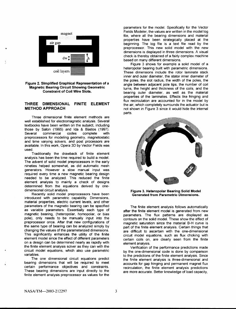
Figure 3 shows for example a solid model of a heteropolar bearing built with parametric dimensions. These dimensions include the rotor laminate stack inner and outer diameter, the stator inner diameter of the poles, the slot radius, the width of the poles, the angle between adjacent pole tips, the number of coil turns, the height and thickness of the coils, and the bearing outer diameter, as well as the material properties of the laminates. Effects like fringing and flux recirculation are accounted for in the model by the air, which completely surrounds the actuator but is not shown in Figure 3 since it would hide the internal parts.

Figure 3. Heteropolar Bearing Solid Model Generated from Parametric Dimensions.

The finite element analysis follows automatically after the finite element model is generated from new parameters. The flux patterns are displayed as contours on the solid model. These show the effect of magnetic saturation since the material B-H curve is part of the finite element analysis. Certain things that are difficult to ascertain with the one-dimensional circuit model equations, such as flux choking with certain coils on, are clearly seen from the finite element analysis.

Verification of the performance predictions made by the one-dimensional code is done by comparison to the predictions of the finite element analysis. Since the finite element analysis is three-dimensional and accounts for gap fringing and permanent magnet flux recirculation, the finite element analysis predictions are more accurate. Better knowledge of load capacity,

3

current and position stiffness, and inductance are thereby obtained.

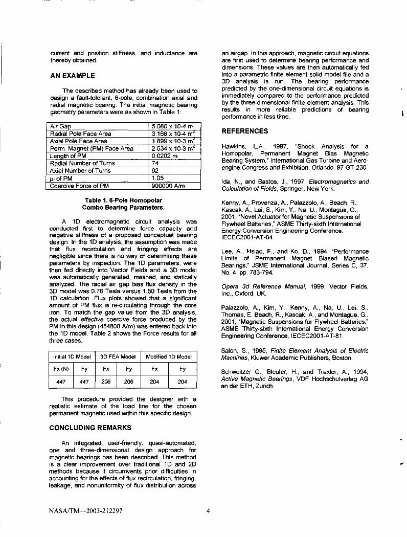
Air Gap Radial Pole Face Area Axial Pole Face Area Perm. Magnet (PM) Face Area Length of PM Radial Number of Turns Axial Number of Turns gr of PM Coercive Force of PM

AN EXAMPLE

5.080 x 10-4 m 3.168 x 10-4 mL 1.899 x 10-3 mL 2.534 x 10-3 mL 0.0202 m 74 92 1.05 900000 N m

The described method has already been used to design a fault-tolerant, 6-pole, combination axial and radial magnetic bearing. The initial magnetic bearing geometry parameters were as shown in Table 1:

an airgap. In this approach, magnetic circuit equations are first used to determine bearing performance and dimensions. These values are then automatically fed into a parametric finite element solid model file and a 3D analysis is run. The bearing performance predicted by the one-dimensional circuit equations is immediately compared to the performance predicted by the three-dimensional finite element analysis. This results in more reliable predictions of bearing performance in less time.

Table 1.6-Pole Homopolar Combo Bearing Parameters.

A I D electromagnetic circuit analysis was conducted first to determine force capacity and negative stiffness of a proposed conceptual bearing design. In the I D analysis, the assumption was made that flux recirculation and fringing effects are negligible since there is no way of determining these parameters by inspection. The 1 D parameters, were then fed directly into Vector Fields and a 3D model was automatically generated, meshed, and statically analyzed. The radial air gap bias flux density in the 3D model was 0.76 Tesla versus 1.50 Tesla from the I D calculation. Flux plots showed that a significant amount of PM flux is re-circulating through the core iron. To match the gap value from the 3D analysis, the actual effective coercive force produced by the PM in this design (454800 Nm) was entered back into the I D model. Table 2 shows the Force results for all three cases.

204 204

This procedure provided the designer with a realistic estimate of the load line for the chosen permanent magnetic used within this specific design.

CONCLUDING REMARKS

An integrated, user-friendly, quasi-automated, one and three-dimensional design approach for magnetic bearings has been described. This method is a clear improvement over traditional I D and 2D methods because it circumvents prior difficulties in accounting for the effects of flux recirculation, fringing, leakage, and nonuniformity of flux distribution across

REFERENCES

Hawkins, L.A., 1997, "Shock Analysis for a Homopolar, Permanent Magnet Bias Magnetic Bearing System," International Gas Turbine and Aero- engine Congress and Exhibition, Orlando, 97-GT-230.

Ida, N., and Bastos, J., 1997, Electromagnetics and Calculation of Fields, Springer, New York.

Kenny, A., Provenza, A., Palazzolo, A., Beach, R., Kascak, A., Lei, S., Kim, Y., Na, U., Montague, G., 2001, "Novel Actuator for Magnetic Suspensions of Flywheel Batteries," ASME Thirty-sixth International Energy Conversion Engineering Conference, I ECEC2001 -AT-84.

Lee, A., Hsiao, F., and KO, D., 1994, "Performance Limits of Permanent Magnet Biased Magnetic Bearings," JSME International Journal, Series C, 37, NO. 4, pp. 783-794.

Opera 3d Reference Manual, 1999, Vector Fields, Inc., Oxford, UK.

Palauolo, A., Kim, Y., Kenny, A., Na, U., Lei, S., Thomas, E. Beach, R., Kascak, A., and Montague, G., 2001, "Magnetic Suspensions for Flywheel Batteries," ASME Thirty-sixth International Energy Conversion Engineering Conference, IECEC2001-AT-81,

Salon, S., 1995, Finite Element Analysis of Electric Machines, Kluwer Academic Publishers, Boston.

Schweitzer G., Bleuler, H., and Traxler, A., 1994, Active Magnetic Bearings, VDF Hochschulverlag AG an der ETH, Zurich.

NASAITM-2003-2 I2297 4

REPORT DOCUMENTATION PAGE

1. AGENCY USE ONLY (Leave blank)

Form Approved OME NO. 0704-0188

2. REPORT DATE 3. REPORT TYPE AND DATES COVERED

April 2003 Technical Memorandum

I

Public reporting burden for this collection of information is estimated to average 1 hour per response, including the time for reviewing instructions, searching existing data sources, gathering and maintaining the data needed, and completing and reviewing the collection of information. Send comments regarding this burden estimate or any other aspect of this collection of information. including suggestions for reducing this burden, to Washington Headquarters Services, Directorate lor Information Operations and Reports, 121 5 Jefferson Davis Highway. Suite 1204. Arlington. VA 22202-4302, and to the Oflice of Management and Budget. Paperwork Reduction Project (0704-0188). Washington. DC 20503.

3. SPONSORlNG/MONlTORlNG AGENCY NAME(S) AND ADDRESS(ES) 10. SPONSORlNG/MONlTORlNG AGENCY REPORT NUMBER

6. AUTHOR(S)

12a. DISTRIBUTIONIAVAILABILITY STATEMENT

Unclassified -Unlimited Subject Category: 44 Distribution: Nonstandard

Available electronically at http://gltrs. prc.nasa.gov This publication is available from the NASA Center for Aerospace Information, 301-6214390.

Andrew J. Provenza, Andrew Kenny, and Alan B. Palazzolo

12b. DISTRIBUTION CODE

7. PERFORMING ORGANIZATION NAME(S) AND ADDRESS(ES)

14. SUBJECT TERMS

Magnetic bearing; Magnetic bearing design; Magnetic circuit model

17. SECURITY CLASSIFICATION 18. SECURITY CLASSIFICATION 19. SECURITY CLASSIFICATION OF REPORT OF THIS PAGE OF ABSTRACT

Unclassified Unclassified Unclassified

National Aeronautics and Space Administration John H. Glenn Research Center at Lewis Field Cleveland, Ohio 44135-3191

15. NUMBER OF PAGES

16. PRICE CODE 10

20. LIMITATION OF ABSTRACT

WBS-22-75741-12

8. PERFORMING ORGANIZATION REPORT NUMBER

E- 13859

National Aeronautics and Space Administration Washington, DC 20546-0001 NASA TM-2003-212297

ICECE-2002-20095

A code for designing magnetic bearings is described. The code generates curves from magnetic circuit equations relating important bearing performance parameters. Bearing parameters selected from the curves by a designer to meet the requirements of a particular application are input directly by the code into a three-dimensional finite element analysis preprocessor. This means that a three-dimensional computer model of the bearing being developed is immedi- ately available for viewing. The finite element model solution can be used to show areas of magnetic saturation and make more accurate predictions of the bearing load capacity, current stiffness, position stiffness, and inductance than the magnetic circuit equations did at the start of the design process. In summary, the code combines one-dimensional and three-dimensional modeling methods for designing magnetic bearings.

NSN 7540-01 -280-5500 Standard Form 298 (Rev. 2-89) Prescribed by ANSI Std. 239-18 298-1 02