An Introduction to Conditional Random Fields

Charles Sutton

University of Edinburgh

csutton@inf.ed.ac.uk

Andrew McCallum

University of Massachusetts Amherst

mccallum@cs.umass.edu

17 November 2010

Abstract

Often we wish to predict a large number of variables that depend on

each other as well as on other observed variables. Structured predic-

tion methods are essentially a combination of classification and graph-

ical modeling, combining the ability of graphical models to compactly

model multivariate data with the ability of classification methods to

perform prediction using large sets of input features. This tutorial de-

scribes conditional random fields, a popular probabilistic method for

structured prediction. CRFs have seen wide application in natural lan-

guage processing, computer vision, and bioinformatics. We describe

methods for inference and parameter estimation for CRFs, including

practical issues for implementing large scale CRFs. We do not assume

previous knowledge of graphical modeling, so this tutorial is intended

to be useful to practitioners in a wide variety of fields.

arX

iv:1

011.

4088

v1 [

stat

.ML

] 1

7 N

ov 2

010

Contents

1 Introduction 1

2 Modeling 5

2.1 Graphical Modeling 6

2.2 Generative versus Discriminative Models 10

2.3 Linear-chain CRFs 18

2.4 General CRFs 21

2.5 Applications of CRFs 23

2.6 Feature Engineering 24

2.7 Notes on Terminology 26

3 Inference 27

3.1 Linear-Chain CRFs 28

3.2 Inference in Graphical Models 32

3.3 Implementation Concerns 40

4 Parameter Estimation 43

i

4.1 Maximum Likelihood 44

4.2 Stochastic Gradient Methods 52

4.3 Parallelism 54

4.4 Approximate Training 54

4.5 Implementation Concerns 61

5 Related Work and Future Directions 63

5.1 Related Work 63

5.2 Frontier Areas 70

1

Introduction

Fundamental to many applications is the ability to predict multiple

variables that depend on each other. Such applications are as diverse

as classifying regions of an image [60], estimating the score in a game

of Go [111], segmenting genes in a strand of DNA [5], and extracting

syntax from natural-language text [123]. In such applications, we wish

to predict a vector y = {y0, y1, . . . , yT } of random variables given an

observed feature vector x. A relatively simple example from natural-

language processing is part-of-speech tagging, in which each variable

ys is the part-of-speech tag of the word at position s, and the input x

is divided into feature vectors {x0,x1 . . .xT }. Each xs contains various

information about the word at position s, such as its identity, ortho-

graphic features such as prefixes and suffixes, membership in domain-

specific lexicons, and information in semantic databases such as Word-

Net.

One approach to this multivariate prediction problem, especially

if our goal is to maximize the number of labels ys that are correctly

classified, is to learn an independent per-position classifier that maps

x 7→ ys for each s. The difficulty, however, is that the output variables

have complex dependencies. For example, neighboring words in a doc-

1

ument or neighboring regions in a image tend to have similar labels.

Or the output variables may represent a complex structure such as a

parse tree, in which a choice of what grammar rule to use near the top

of the tree can have a large effect on the rest of the tree.

A natural way to represent the manner in which output variables

depend on each other is provided by graphical models. Graphical

models—which include such diverse model families as Bayesian net-

works, neural networks, factor graphs, Markov random fields, Ising

models, and others—represent a complex distribution over many vari-

ables as a product of local factors on smaller subsets of variables. It

is then possible to describe how a given factorization of the proba-

bility density corresponds to a particular set of conditional indepen-

dence relationships satisfied by the distribution. This correspondence

makes modeling much more convenient, because often our knowledge of

the domain suggests reasonable conditional independence assumptions,

which then determine our choice of factors.

Much work in learning with graphical models, especially in statisti-

cal natural-language processing, has focused on generative models that

explicitly attempt to model a joint probability distribution p(y,x) over

inputs and outputs. Although there are advantages to this approach, it

also has important limitations. Not only can the dimensionality of x be

very large, but the features have complex dependencies, so constructing

a probability distribution over them is difficult. Modelling the depen-

dencies among inputs can lead to intractable models, but ignoring them

can lead to reduced performance.

A solution to this problem is to model the conditional distribution

p(y|x) directly, which is all that is needed for classification. This is a

conditional random field (CRF). CRFs are essentially a way of combin-

ing the advantages of classification and graphical modeling, combining

the ability to compactly model multivariate data with the ability to

leverage a large number of input features for prediction. The advantage

to a conditional model is that dependencies that involve only variables

in x play no role in the conditional model, so that an accurate con-

ditional model can have much simpler structure than a joint model.

The difference between generative models and CRFs is thus exactly

analogous to the difference between the naive Bayes and logistic re-

gression classifiers. Indeed, the multinomial logistic regression model

can be seen as the simplest kind of CRF, in which there is only one

output variable.

There has been a large amount of applied interest in CRFs. Suc-

cessful applications have included text processing [89, 107, 108], bioin-

formatics [106, 65], and computer vision [43, 53]. Although early appli-

cations of CRFs used linear chains, recent applications of CRFs have

also used more general graphical structures. General graphical struc-

tures are useful for predicting complex structures, such as graphs and

trees, and for relaxing the iid assumption among entities, as in rela-

tional learning [121].

This tutorial describes modeling, inference, and parameter estima-

tion using conditional random fields. We do not assume previous knowl-

edge of graphical modeling, so this tutorial is intended to be useful to

practitioners in a wide variety of fields. We begin by describing mod-

elling issues in CRFs (Chapter 2), including linear-chain CRFs, CRFs

with general graphical structure, and hidden CRFs that include latent

variables. We describe how CRFs can be viewed both as a generaliza-

tion of the well-known logistic regression procedure, and as a discrimi-

native analogue of the hidden Markov model.

In the next two chapters, we describe inference (Chapter 3) and

learning (Chapter 4) in CRFs. The two procedures are closely coupled,

because learning usually calls inference as a subroutine. Although the

inference algorithms that we discuss are standard algorithms for graph-

ical models, the fact that inference is embedded within an outer param-

eter estimation procedure raises additional issues. Finally, we discuss

relationships between CRFs and other families of models, including

other structured prediction methods, neural networks, and maximum

entropy Markov models (Chapter 5).

Implementation Details

Throughout this monograph, we try to point out implementation de-

tails that are sometimes elided in the research literature. For example,

we discuss issues relating to feature engineering (Section 2.6), avoiding

numerical overflow during inference (Section 3.3), and the scalability

of CRF training on some benchmark problems (Section 4.5).

Since this is the first of our sections on implementation details, it

seems appropriate to mention some of the available implementations of

CRFs. At the time of writing, a few popular implementations are:

CRF++ http://crfpp.sourceforge.net/

MALLET http://mallet.cs.umass.edu/

GRMM http://mallet.cs.umass.edu/grmm/

CRFSuite http://www.chokkan.org/software/crfsuite/

FACTORIE http://www.factorie.cc

Also, software for Markov Logic networks (such as Alchemy: http:

//alchemy.cs.washington.edu/) can be used to build CRF models.

Alchemy, GRMM, and FACTORIE are the only toolkits of which we

are aware that handle arbitrary graphical structure.

2

Modeling

In this chapter, we describe conditional random fields from a model-

ing perspective, explaining how a CRF represents distributions over

structured outputs as a function of a high-dimensional input vector.

CRFs can be understood both as an extension of the logistic regression

classifier to arbitrary graphical structures, or as a discriminative ana-

log of generative models of structured data, an such as hidden Markov

models.

We begin with a brief introduction to graphical modeling (Sec-

tion 2.1) and a description of generative and discriminative models

in NLP (Section 2.2). Then we will be able to present the formal defi-

nition of conditional random field, both for the commonly-used case of

linear chains (Section 2.3), and for general graphical structures (Sec-

tion 2.4). Finally, we present some examples of how different structures

are used in applications (Section 2.5), and some implementation details

concerning feature engineering (Section 2.6).

5

2.1 Graphical Modeling

Graphical modeling is a powerful framework for representation and

inference in multivariate probability distributions. It has proven useful

in diverse areas of stochastic modeling, including coding theory [77],

computer vision [34], knowledge representation [88], Bayesian statistics

[33], and natural-language processing [54, 9].

Distributions over many variables can be expensive to represent

naıvely. For example, a table of joint probabilities of n binary vari-

ables requires storing O(2n) floating-point numbers. The insight of the

graphical modeling perspective is that a distribution over very many

variables can often be represented as a product of local functions that

each depend on a much smaller subset of variables. This factorization

turns out to have a close connection to certain conditional indepen-

dence relationships among the variables—both types of information

being easily summarized by a graph. Indeed, this relationship between

factorization, conditional independence, and graph structure comprises

much of the power of the graphical modeling framework: the condi-

tional independence viewpoint is most useful for designing models, and

the factorization viewpoint is most useful for designing inference algo-

rithms.

In the rest of this section, we introduce graphical models from both

the factorization and conditional independence viewpoints, focusing on

those models which are based on undirected graphs. A more detailed

modern perspective on graphical modelling and approximate inference

is available in a textbook by Koller and Friedman [49].

2.1.1 Undirected Models

We consider probability distributions over sets of random variables V =

X∪Y , where X is a set of input variables that we assume are observed,

and Y is a set of output variables that we wish to predict. Every variable

s ∈ V takes outcomes from a set V, which can be either continuous or

discrete, although we consider only the discrete case in this tutorial. An

arbitrary assignment to X is denoted by a vector x. Given a variable

s ∈ X, the notation xs denotes the value assigned to s by x, and

similarly for an assignment to a subset a ⊂ X by xa. The notation

1{x=x′} denotes an indicator function of x which takes the value 1 when

x = x′ and 0 otherwise. We also require notation for marginalization.

For a fixed variable assignment ys, we use the summation∑

y\ys to

indicate a summation over all possible assignments y whose value for

variable s is equal to ys.

Suppose that we believe that a probability distribution p of interest

can be represented by a product of factors of the form Ψa(xa,ya),

where each factor has scope a ⊆ V . This factorization can allow us

to represent p much more efficiently, because the sets a may be much

smaller than the full variable set V . We assume that without loss of

generality that each distinct set a has at most one factor Ψa.

An undirected graphical model is a family of probability distribu-

tions that factorize according to given collection of scopes. Formally,

given a collection of subsets F = a ⊂ V , an undirected graphical model

is defined as the set of all distributions that can be written in the form

p(x,y) =1

Z

∏a∈F

Ψa(xa,ya), (2.1)

for any choice of local function F = {Ψa}, where Ψa : V |a| → <+.

(These functions are also called factors or compatibility functions.) We

will occasionally use the term random field to refer to a particular

distribution among those defined by an undirected model. The reason

for the term graphical model will become apparent shortly, when we

discuss how the factorization of (2.1) can be represented as a graph.

The constant Z is a normalization factor that ensures the distribu-

tion p sums to 1. It is defined as

Z =∑x,y

∏a∈F

Ψa(xa,ya). (2.2)

The quantity Z, considered as a function of the set F of factors, is

sometime called the partition function. Notice that the summation in

(2.2) is over the exponentially many possible assignments to x and y.

For this reason, computing Z is intractable in general, but much work

exists on how to approximate it.

We will generally assume further that each local function has the

form

Ψa(xa,ya) = exp

{∑k

θakfak(xa,ya)

}, (2.3)

for some real-valued parameter vector θa, and for some set of feature

functions or sufficient statistics {fak}. If x and y are discrete, then this

assumption is without loss of generality, because we can have features

have indicator functions for every possible value, that is, if we include

one feature function fak(xa,ya) = 1{xa=x∗a}1{ya=y∗a} for every possible

value x∗a and y∗a.

Also, a consequence of this parameterization is that the family of

distributions over V parameterized by θ is an exponential family. In-

deed, much of the discussion in this tutorial about parameter estimation

for CRFs applies to exponential families in general.

As we have mentioned, there is a close connection between the

factorization of a graphical model and the conditional independencies

among the variables in its domain. This connection can be understood

by means of an undirected graph known as a Markov network, which

directly represents conditional independence relationships in a multi-

variate distribution. Let G be an undirected graph with variables V ,

that is, G has one node for every random variable of interest. For a

variable s ∈ V , let N(s) denote the neighbors of s. Then we say that a

distribution p is Markov with respect to G if it meets the local Markov

property: for any two variables s, t ∈ V , the variable s is independent

of t conditioned on its neighbors N(s). Intuitively, this means that the

neighbors of s contain all of the information necessary to predict its

value.

Given a factorization of a distribution p as in (2.1), an equivalent

Markov network can be constructed by connecting all pairs of variables

that share a local function. It is straightforward to show that p is

Markov with respect to this graph, because the conditional distribution

p(xs|xN(s)) that follows from (2.1) is a function only of variables that

appear in the Markov blanket. In other words, if p factorizes according

to G, then p is Markov with respect to G.

The converse direction also holds, as long as p is strictly positive.

This is stated in the following classical result [42, 7]:

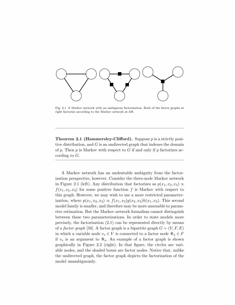
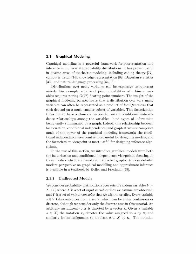
Fig. 2.1 A Markov network with an ambiguous factorization. Both of the factor graphs at

right factorize according to the Markov network at left.

Theorem 2.1 (Hammersley-Clifford). Suppose p is a strictly posi-

tive distribution, and G is an undirected graph that indexes the domain

of p. Then p is Markov with respect to G if and only if p factorizes ac-

cording to G.

A Markov network has an undesirable ambiguity from the factor-

ization perspective, however. Consider the three-node Markov network

in Figure 2.1 (left). Any distribution that factorizes as p(x1, x2, x3) ∝f(x1, x2, x3) for some positive function f is Markov with respect to

this graph. However, we may wish to use a more restricted parameter-

ization, where p(x1, x2, x3) ∝ f(x1, x2)g(x2, x3)h(x1, x3). This second

model family is smaller, and therefore may be more amenable to param-

eter estimation. But the Markov network formalism cannot distinguish

between these two parameterizations. In order to state models more

precisely, the factorization (2.1) can be represented directly by means

of a factor graph [50]. A factor graph is a bipartite graph G = (V, F,E)

in which a variable node vs ∈ V is connected to a factor node Ψa ∈ Fif vs is an argument to Ψa. An example of a factor graph is shown

graphically in Figure 2.2 (right). In that figure, the circles are vari-

able nodes, and the shaded boxes are factor nodes. Notice that, unlike

the undirected graph, the factor graph depicts the factorization of the

model unambiguously.

2.1.2 Directed Models

Whereas the local functions in an undirected model need not have a

direct probabilistic interpretation, a directed graphical model describes

how a distribution factorizes into local conditional probability distri-

butions. Let G = (V,E) be a directed acyclic graph, in which π(v)

are the parents of v in G. A directed graphical model is a family of

distributions that factorize as:

p(y,x) =∏v∈V

p(yv|yπ(v)). (2.4)

It can be shown by structural induction on G that p is properly normal-

ized. Directed models can be thought of as a kind of factor graph, in

which the individual factors are locally normalized in a special fashion

so that globally Z = 1. Directed models are often used as generative

models, as we explain in Section 2.2.3. An example of a directed model

is the naive Bayes model (2.5), which is depicted graphically in Fig-

ure 2.2 (left).

2.2 Generative versus Discriminative Models

In this section we discuss several examples applications of simple graph-

ical models to natural language processing. Although these examples

are well-known, they serve both to clarify the definitions in the pre-

vious section, and to illustrate some ideas that will arise again in our

discussion of conditional random fields. We devote special attention to

the hidden Markov model (HMM), because it is closely related to the

linear-chain CRF.

2.2.1 Classification

First we discuss the problem of classification, that is, predicting a single

discrete class variable y given a vector of features x = (x1, x2, . . . , xK).

One simple way to accomplish this is to assume that once the class

label is known, all the features are independent. The resulting classifier

is called the naive Bayes classifier. It is based on a joint probability

x

y

x

y

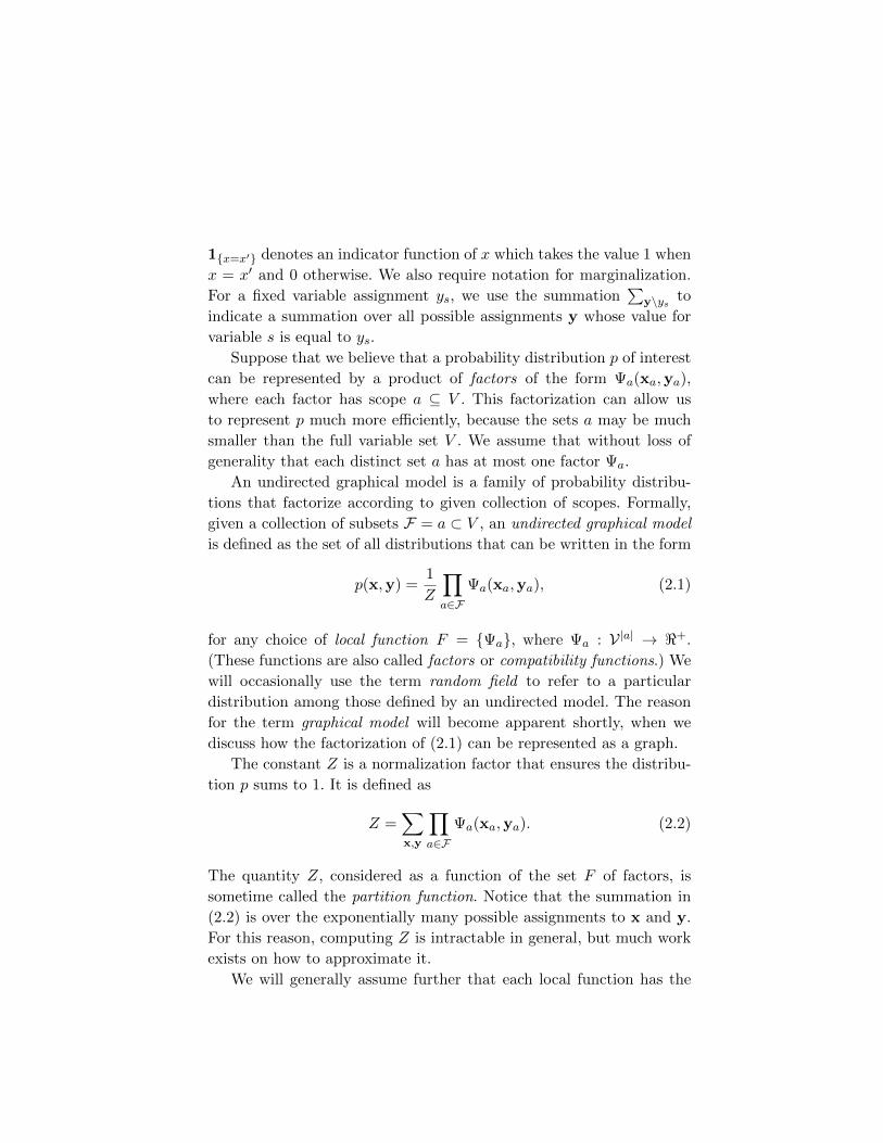
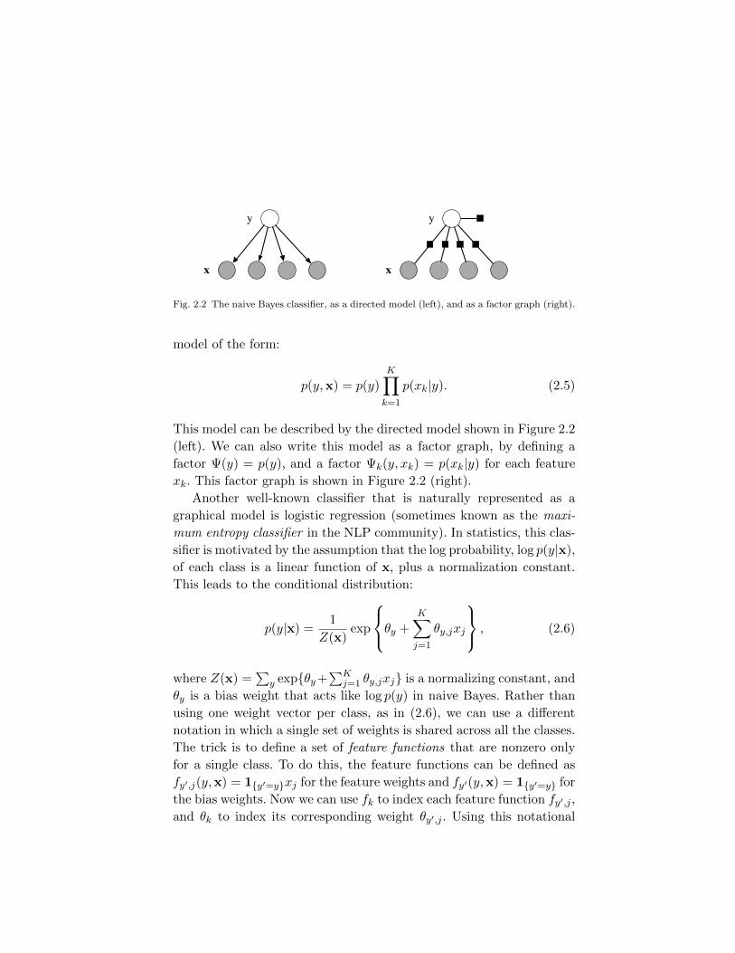
Fig. 2.2 The naive Bayes classifier, as a directed model (left), and as a factor graph (right).

model of the form:

p(y,x) = p(y)

K∏k=1

p(xk|y). (2.5)

This model can be described by the directed model shown in Figure 2.2

(left). We can also write this model as a factor graph, by defining a

factor Ψ(y) = p(y), and a factor Ψk(y, xk) = p(xk|y) for each feature

xk. This factor graph is shown in Figure 2.2 (right).

Another well-known classifier that is naturally represented as a

graphical model is logistic regression (sometimes known as the maxi-

mum entropy classifier in the NLP community). In statistics, this clas-

sifier is motivated by the assumption that the log probability, log p(y|x),

of each class is a linear function of x, plus a normalization constant.

This leads to the conditional distribution:

p(y|x) =1

Z(x)exp

θy +K∑j=1

θy,jxj

, (2.6)

where Z(x) =∑

y exp{θy+∑K

j=1 θy,jxj} is a normalizing constant, and

θy is a bias weight that acts like log p(y) in naive Bayes. Rather than

using one weight vector per class, as in (2.6), we can use a different

notation in which a single set of weights is shared across all the classes.

The trick is to define a set of feature functions that are nonzero only

for a single class. To do this, the feature functions can be defined as

fy′,j(y,x) = 1{y′=y}xj for the feature weights and fy′(y,x) = 1{y′=y} for

the bias weights. Now we can use fk to index each feature function fy′,j ,

and θk to index its corresponding weight θy′,j . Using this notational

trick, the logistic regression model becomes:

p(y|x) =1

Z(x)exp

{K∑k=1

θkfk(y,x)

}. (2.7)

We introduce this notation because it mirrors the notation for condi-

tional random fields that we will present later.

2.2.2 Sequence Models

Classifiers predict only a single class variable, but the true power of

graphical models lies in their ability to model many variables that

are interdependent. In this section, we discuss perhaps the simplest

form of dependency, in which the output variables are arranged in a

sequence. To motivate this kind of model, we discuss an application

from natural language processing, the task of named-entity recognition

(NER). NER is the problem of identifying and classifying proper names

in text, including locations, such as China; people, such as George

Bush; and organizations, such as the United Nations. The named-entity

recognition task is, given a sentence, to segment which words are part

of entities, and to classify each entity by type (person, organization,

location, and so on). The challenge of this problem is that many named

entities are too rare to appear even in a large training set, and therefore

the system must identify them based only on context.

One approach to NER is to classify each word independently as one

of either Person, Location, Organization, or Other (meaning

not an entity). The problem with this approach is that it assumes

that given the input, all of the named-entity labels are independent.

In fact, the named-entity labels of neighboring words are dependent;

for example, while New York is a location, New York Times is an

organization. One way to relax this independence assumption is to

arrange the output variables in a linear chain. This is the approach

taken by the hidden Markov model (HMM) [96]. An HMM models a

sequence of observations X = {xt}Tt=1 by assuming that there is an

underlying sequence of states Y = {yt}Tt=1 drawn from a finite state

set S. In the named-entity example, each observation xt is the identity

of the word at position t, and each state yt is the named-entity label,

that is, one of the entity types Person, Location, Organization,

and Other.

To model the joint distribution p(y,x) tractably, an HMM makes

two independence assumptions. First, it assumes that each state de-

pends only on its immediate predecessor, that is, each state yt is in-

dependent of all its ancestors y1, y2, . . . , yt−2 given the preceding state

yt−1. Second, it also assumes that each observation variable xt depends

only on the current state yt. With these assumptions, we can specify an

HMM using three probability distributions: first, the distribution p(y1)

over initial states; second, the transition distribution p(yt|yt−1); and

finally, the observation distribution p(xt|yt). That is, the joint proba-

bility of a state sequence y and an observation sequence x factorizes

as

p(y,x) =

T∏t=1

p(yt|yt−1)p(xt|yt), (2.8)

where, to simplify notation, we write the initial state distribution p(y1)

as p(y1|y0). In natural language processing, HMMs have been used for

sequence labeling tasks such as part-of-speech tagging, named-entity

recognition, and information extraction.

2.2.3 Comparison

Of the models described in this section, two are generative (the naive

Bayes and hidden Markov models) and one is discriminative (the lo-

gistic regression model). In a general, generative models are models

of the joint distribution p(y,x), and like naive Bayes have the form

p(y)p(x|y). In other words, they describe how the output is probabilis-

tically generated as a function of the input. Discriminative models, on

the other hand, focus solely on the conditional distribution p(y|x). In

this section, we discuss the differences between generative and discrim-

inative modeling, and the potential advantages of discriminative mod-

eling. For concreteness, we focus on the examples of naive Bayes and

logistic regression, but the discussion in this section applies equally as

well to the differences between arbitrarily structured generative models

and conditional random fields.

The main difference is that a conditional distribution p(y|x) does

not include a model of p(x), which is not needed for classification any-

way. The difficulty in modeling p(x) is that it often contains many

highly dependent features that are difficult to model. For example,

in named-entity recognition, an HMM relies on only one feature, the

word’s identity. But many words, especially proper names, will not have

occurred in the training set, so the word-identity feature is uninforma-

tive. To label unseen words, we would like to exploit other features of a

word, such as its capitalization, its neighboring words, its prefixes and

suffixes, its membership in predetermined lists of people and locations,

and so on.

The principal advantage of discriminative modeling is that it is bet-

ter suited to including rich, overlapping features. To understand this,

consider the family of naive Bayes distributions (2.5). This is a family

of joint distributions whose conditionals all take the “logistic regression

form” (2.7). But there are many other joint models, some with com-

plex dependencies among x, whose conditional distributions also have

the form (2.7). By modeling the conditional distribution directly, we

can remain agnostic about the form of p(x). CRFs make independence

assumptions among y, and assumptions about how the y can depend

on x, but not among x. This point can also be understood graphi-

cally: Suppose that we have a factor graph representation for the joint

distribution p(y,x). If we then construct a graph for the conditional

distribution p(y|x), any factors that depend only on x vanish from the

graphical structure for the conditional distribution. They are irrelevant

to the conditional because they are constant with respect to y.

To include interdependent features in a generative model, we have

two choices: enhance the model to represent dependencies among the in-

puts, or make simplifying independence assumptions, such as the naive

Bayes assumption. The first approach, enhancing the model, is often

difficult to do while retaining tractability. For example, it is hard to

imagine how to model the dependence between the capitalization of a

word and its suffixes, nor do we particularly wish to do so, since we

always observe the test sentences anyway. The second approach—to in-

clude a large number of dependent features in a generative model, but

to include independence assumptions among them—is possible, and in

some domains can work well. But it can also be problematic because

the independence assumptions can hurt performance. For example, al-

though the naive Bayes classifier performs well in document classifica-

tion, it performs worse on average across a range of applications than

logistic regression [16].

Furthermore, naive Bayes can produce poor probability esti-

mates. As an illustrative example, imagine training naive Bayes on

a data set in which all the features are repeated, that is, x =

(x1, x1, x2, x2, . . . , xK , xK). This will increase the confidence of the

naive Bayes probability estimates, even though no new information

has been added to the data. Assumptions like naive Bayes can be espe-

cially problematic when we generalize to sequence models, because in-

ference essentially combines evidence from different parts of the model.

If probability estimates of the label at each sequence position are over-

confident, it might be difficult to combine them sensibly.

The difference between naive Bayes and logistic regression is due

only to the fact that the first is generative and the second discrimi-

native; the two classifiers are, for discrete input, identical in all other

respects. Naive Bayes and logistic regression consider the same hy-

pothesis space, in the sense that any logistic regression classifier can be

converted into a naive Bayes classifier with the same decision boundary,

and vice versa. Another way of saying this is that the naive Bayes model

(2.5) defines the same family of distributions as the logistic regression

model (2.7), if we interpret it generatively as

p(y,x) =exp {

∑k θkfk(y,x)}∑

y,x exp {∑

k θkfk(y, x)}. (2.9)

This means that if the naive Bayes model (2.5) is trained to maximize

the conditional likelihood, we recover the same classifier as from logis-

tic regression. Conversely, if the logistic regression model is interpreted

generatively, as in (2.9), and is trained to maximize the joint likelihood

p(y,x), then we recover the same classifier as from naive Bayes. In the

terminology of Ng and Jordan [85], naive Bayes and logistic regression

form a generative-discriminative pair. For a recent theoretical perspec-

tive on generative and discriminative models, see Liang and Jordan

[61].

Logistic Regression

HMMs

Linear-chain CRFs

Naive BayesSEQUENCE

SEQUENCE

CONDITIONAL CONDITIONAL

Generative directed models

General CRFs

CONDITIONAL

GeneralGRAPHS

GeneralGRAPHS

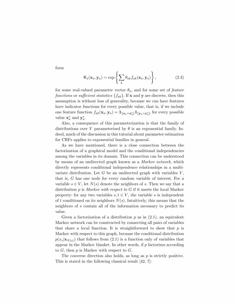
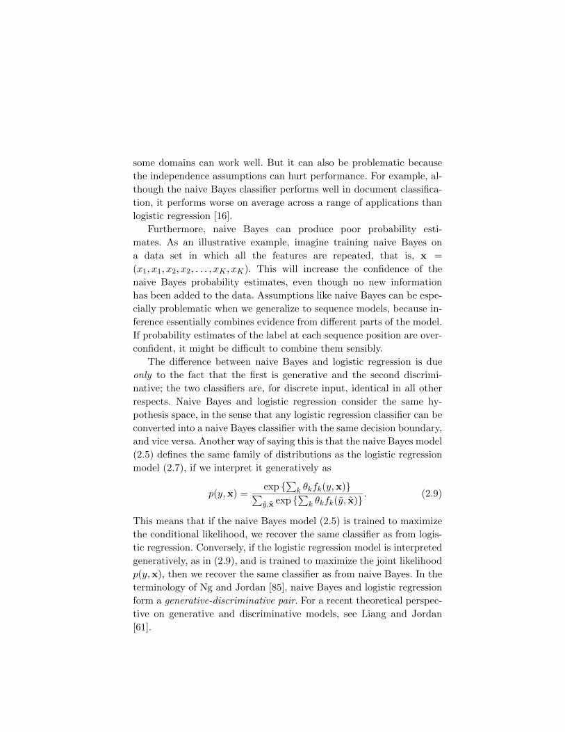
Fig. 2.3 Diagram of the relationship between naive Bayes, logistic regression, HMMs, linear-chain CRFs, generative models, and general CRFs.

One perspective for gaining insight into the difference between gen-

erative and discriminative modeling is due to Minka [80]. Suppose we

have a generative model pg with parameters θ. By definition, this takes

the form

pg(y,x; θ) = pg(y; θ)pg(x|y; θ). (2.10)

But we could also rewrite pg using Bayes rule as

pg(y,x; θ) = pg(x; θ)pg(y|x; θ), (2.11)

where pg(x; θ) and pg(y|x; θ) are computed by inference, i.e., pg(x; θ) =∑y pg(y,x; θ) and pg(y|x; θ) = pg(y,x; θ)/pg(x; θ).

Now, compare this generative model to a discriminative model over

the same family of joint distributions. To do this, we define a prior

p(x) over inputs, such that p(x) could have arisen from pg with some

parameter setting. That is, p(x) = pc(x; θ′) =∑

y pg(y,x|θ′). We com-

bine this with a conditional distribution pc(y|x; θ) that could also have

arisen from pg, that is, pc(y|x; θ) = pg(y,x; θ)/pg(x; θ). Then the re-

sulting distribution is

pc(y,x) = pc(x; θ′)pc(y|x; θ). (2.12)

By comparing (2.11) with (2.12), it can be seen that the conditional

approach has more freedom to fit the data, because it does not require

that θ = θ′. Intuitively, because the parameters θ in (2.11) are used

in both the input distribution and the conditional, a good set of pa-

rameters must represent both well, potentially at the cost of trading

off accuracy on p(y|x), the distribution we care about, for accuracy

on p(x), which we care less about. On the other hand, this added free-

dom brings about an increased risk of overfitting the training data, and

generalizing worse on unseen data.

To be fair, however, generative models have several advantages of

their own. First, generative models can be more natural for handling la-

tent variables, partially-labeled data, and unlabelled data. In the most

extreme case, when the data is entirely unlabeled, generative models

can be applied in an unsupervised fashion, whereas unsupervised learn-

ing in discriminative models is less natural and is still an active area

of research.

Second, on some data a generative model can perform better than

a discriminative model, intuitively because the input model p(x) may

have a smoothing effect on the conditional. Ng and Jordan [85] argue

that this effect is especially pronounced when the data set is small. For

any particular data set, it is impossible to predict in advance whether

a generative or a discriminative model will perform better. Finally,

sometimes either the problem suggests a natural generative model, or

the application requires the ability to predict both future inputs and

future outputs, making a generative model preferable.

Because a generative model takes the form p(y,x) = p(y)p(x|y),

it is often natural to represent a generative model by a directed graph

in which in outputs y topologically precede the inputs. Similarly, we

will see that it is often natural to represent a discriminative model by

a undirected graph, although this need not always be the case.

The relationship between naive Bayes and logistic regression mirrors

the relationship between HMMs and linear-chain CRFs. Just as naive

Bayes and logistic regression are a generative-discriminative pair, there

is a discriminative analogue to the hidden Markov model, and this

analogue is a particular special case of conditional random field, as we

explain in the next section. This analogy between naive Bayes, logistic

regression, generative models, and conditional random fields is depicted

. . .

. . .

y

x

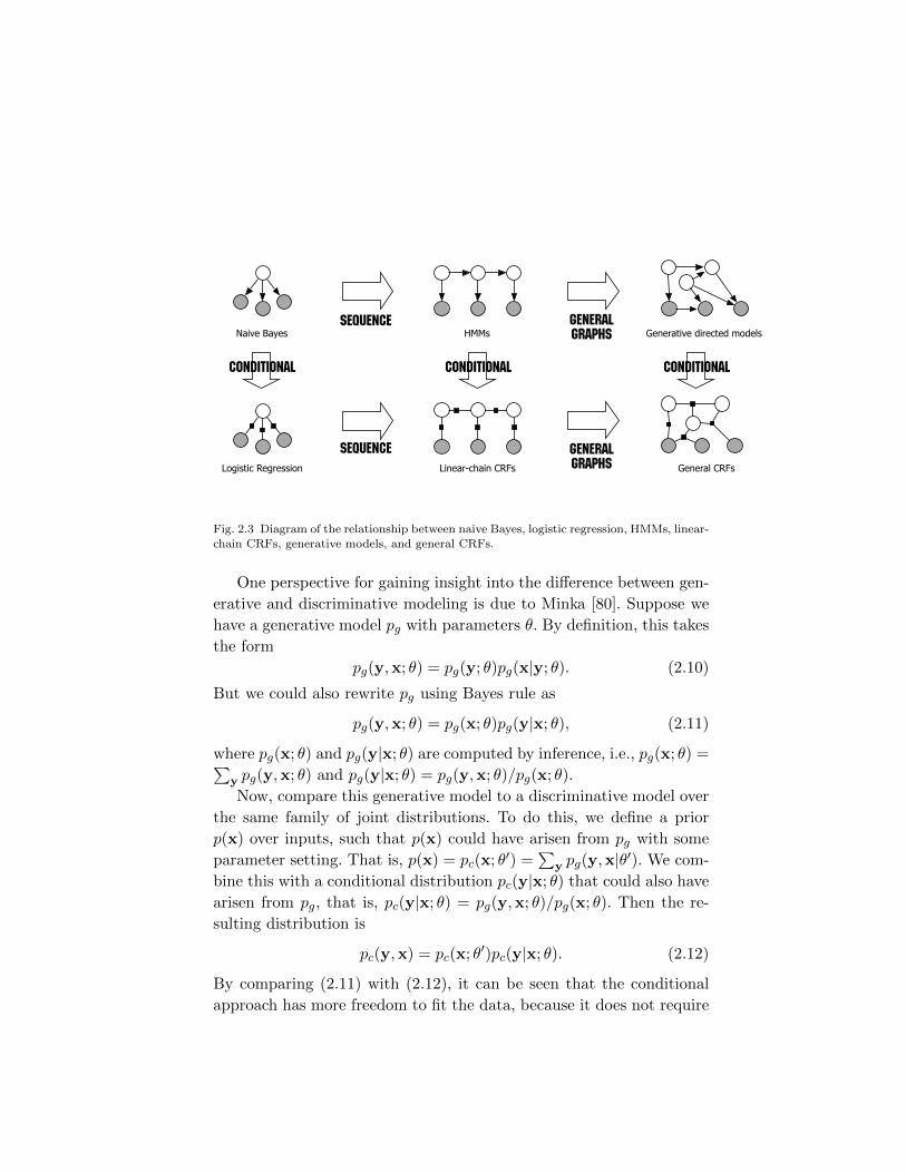
Fig. 2.4 Graphical model of an HMM-like linear-chain CRF.

. . .

. . .

y

x

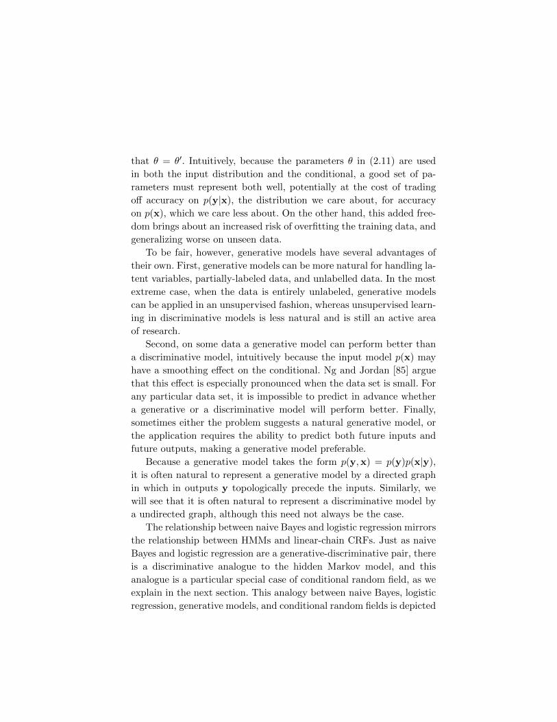
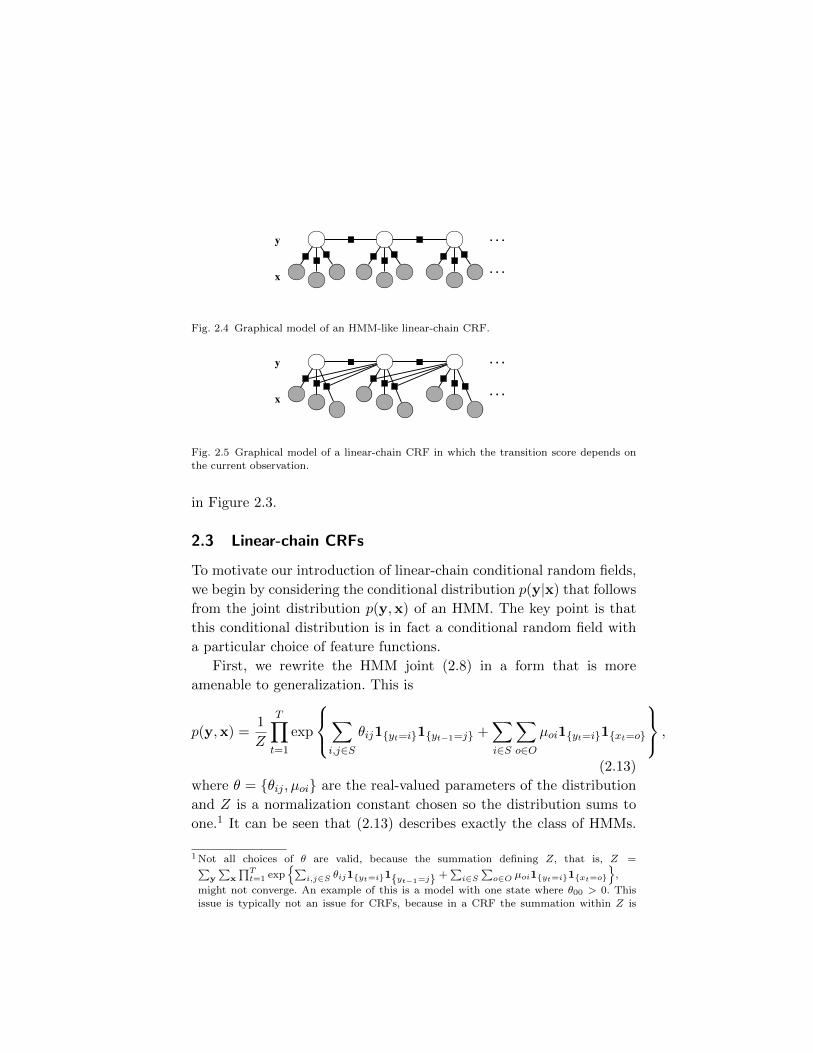
Fig. 2.5 Graphical model of a linear-chain CRF in which the transition score depends on

the current observation.

in Figure 2.3.

2.3 Linear-chain CRFs

To motivate our introduction of linear-chain conditional random fields,

we begin by considering the conditional distribution p(y|x) that follows

from the joint distribution p(y,x) of an HMM. The key point is that

this conditional distribution is in fact a conditional random field with

a particular choice of feature functions.

First, we rewrite the HMM joint (2.8) in a form that is more

amenable to generalization. This is

p(y,x) =1

Z

T∏t=1

exp

∑i,j∈S

θij1{yt=i}1{yt−1=j} +∑i∈S

∑o∈O

µoi1{yt=i}1{xt=o}

,

(2.13)

where θ = {θij , µoi} are the real-valued parameters of the distribution

and Z is a normalization constant chosen so the distribution sums to

one.1 It can be seen that (2.13) describes exactly the class of HMMs.

1Not all choices of θ are valid, because the summation defining Z, that is, Z =∑y

∑x

∏Tt=1 exp

{∑i,j∈S θij1{yt=i}1{yt−1=j} +

∑i∈S

∑o∈O µoi1{yt=i}1{xt=o}

},

might not converge. An example of this is a model with one state where θ00 > 0. Thisissue is typically not an issue for CRFs, because in a CRF the summation within Z is

Every HMM can be written in this form by setting θij = log p(y′ =

i|y = j) and µoi = log p(x = o|y = i). The converse direction is more

complicated, and not relevant for our purposes here. The main point

is that despite this added flexibility in the parameterization (2.13), we

have not added any distributions to the family.

We can write (2.13) more compactly by introducing the concept of

feature functions, just as we did for logistic regression in (2.7). Each fea-

ture function has the form fk(yt, yt−1, xt). In order to duplicate (2.13),

there needs to be one feature fij(y, y′, x) = 1{y=i}1{y′=j} for each tran-

sition (i, j) and one feature fio(y, y′, x) = 1{y=i}1{x=o} for each state-

observation pair (i, o). We refer to a feature function generically as fk,

where fk ranges over both all of the fij and all of the fio. Then we can

write an HMM as:

p(y,x) =1

Z

T∏t=1

exp

{K∑k=1

θkfk(yt, yt−1, xt)

}. (2.14)

Again, equation (2.14) defines exactly the same family of distributions

as (2.13), and therefore as the original HMM equation (2.8).

The last step is to write the conditional distribution p(y|x) that

results from the HMM (2.14). This is

p(y|x) =p(y,x)∑y′ p(y

′,x)=

∏Tt=1 exp

{∑Kk=1 θkfk(yt, yt−1, xt)

}∑

y′∏Tt=1 exp

{∑Kk=1 θkfk(y

′t, y′t−1, xt)

} .(2.15)

This conditional distribution (2.15) is a particular kind of linear-chain

CRF, namely, one that includes features only for the current word’s

identity. But many other linear-chain CRFs use richer features of the

input, such as prefixes and suffixes of the current word, the identity of

surrounding words, and so on. Fortunately, this extension requires little

change to our existing notation. We simply allow the feature functions

to be more general than indicator functions of the word’s identity. This

leads to the general definition of linear-chain CRFs:

usually over a finite set.

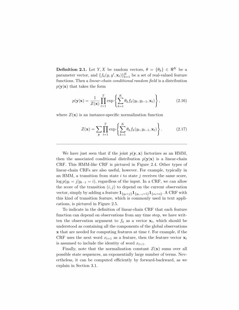
Definition 2.1. Let Y,X be random vectors, θ = {θk} ∈ <K be a

parameter vector, and {fk(y, y′,xt)}Kk=1 be a set of real-valued feature

functions. Then a linear-chain conditional random field is a distribution

p(y|x) that takes the form

p(y|x) =1

Z(x)

T∏t=1

exp

{K∑k=1

θkfk(yt, yt−1,xt)

}, (2.16)

where Z(x) is an instance-specific normalization function

Z(x) =∑y

T∏t=1

exp

{K∑k=1

θkfk(yt, yt−1,xt)

}. (2.17)

We have just seen that if the joint p(y,x) factorizes as an HMM,

then the associated conditional distribution p(y|x) is a linear-chain

CRF. This HMM-like CRF is pictured in Figure 2.4. Other types of

linear-chain CRFs are also useful, however. For example, typically in

an HMM, a transition from state i to state j receives the same score,

log p(yt = j|yt−1 = i), regardless of the input. In a CRF, we can allow

the score of the transition (i, j) to depend on the current observation

vector, simply by adding a feature 1{yt=j}1{yt−1=1}1{xt=o}. A CRF with

this kind of transition feature, which is commonly used in text appli-

cations, is pictured in Figure 2.5.

To indicate in the definition of linear-chain CRF that each feature

function can depend on observations from any time step, we have writ-

ten the observation argument to fk as a vector xt, which should be

understood as containing all the components of the global observations

x that are needed for computing features at time t. For example, if the

CRF uses the next word xt+1 as a feature, then the feature vector xtis assumed to include the identity of word xt+1.

Finally, note that the normalization constant Z(x) sums over all

possible state sequences, an exponentially large number of terms. Nev-

ertheless, it can be computed efficiently by forward-backward, as we

explain in Section 3.1.

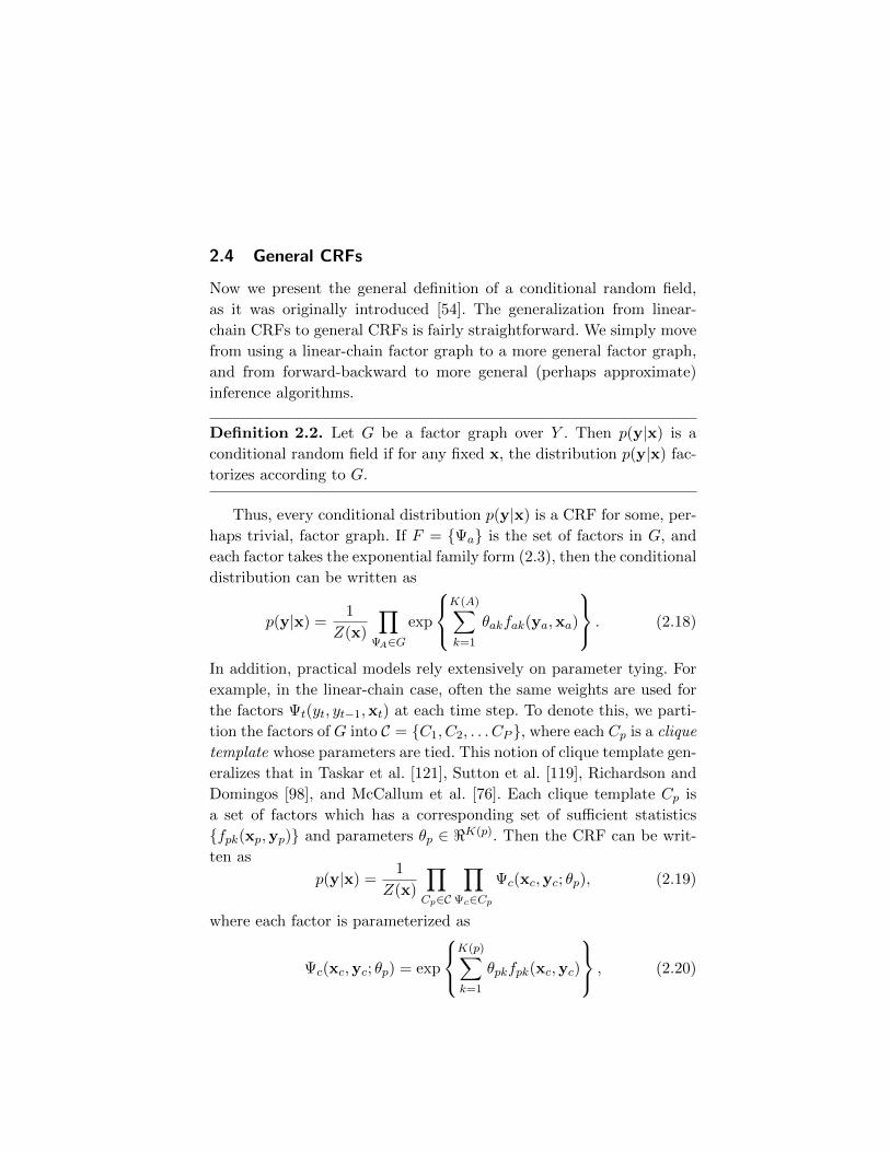
2.4 General CRFs

Now we present the general definition of a conditional random field,

as it was originally introduced [54]. The generalization from linear-

chain CRFs to general CRFs is fairly straightforward. We simply move

from using a linear-chain factor graph to a more general factor graph,

and from forward-backward to more general (perhaps approximate)

inference algorithms.

Definition 2.2. Let G be a factor graph over Y . Then p(y|x) is a

conditional random field if for any fixed x, the distribution p(y|x) fac-

torizes according to G.

Thus, every conditional distribution p(y|x) is a CRF for some, per-

haps trivial, factor graph. If F = {Ψa} is the set of factors in G, and

each factor takes the exponential family form (2.3), then the conditional

distribution can be written as

p(y|x) =1

Z(x)

∏ΨA∈G

exp

K(A)∑k=1

θakfak(ya,xa)

. (2.18)

In addition, practical models rely extensively on parameter tying. For

example, in the linear-chain case, often the same weights are used for

the factors Ψt(yt, yt−1,xt) at each time step. To denote this, we parti-

tion the factors of G into C = {C1, C2, . . . CP }, where each Cp is a clique

template whose parameters are tied. This notion of clique template gen-

eralizes that in Taskar et al. [121], Sutton et al. [119], Richardson and

Domingos [98], and McCallum et al. [76]. Each clique template Cp is

a set of factors which has a corresponding set of sufficient statistics

{fpk(xp,yp)} and parameters θp ∈ <K(p). Then the CRF can be writ-

ten as

p(y|x) =1

Z(x)

∏Cp∈C

∏Ψc∈Cp

Ψc(xc,yc; θp), (2.19)

where each factor is parameterized as

Ψc(xc,yc; θp) = exp

K(p)∑k=1

θpkfpk(xc,yc)

, (2.20)

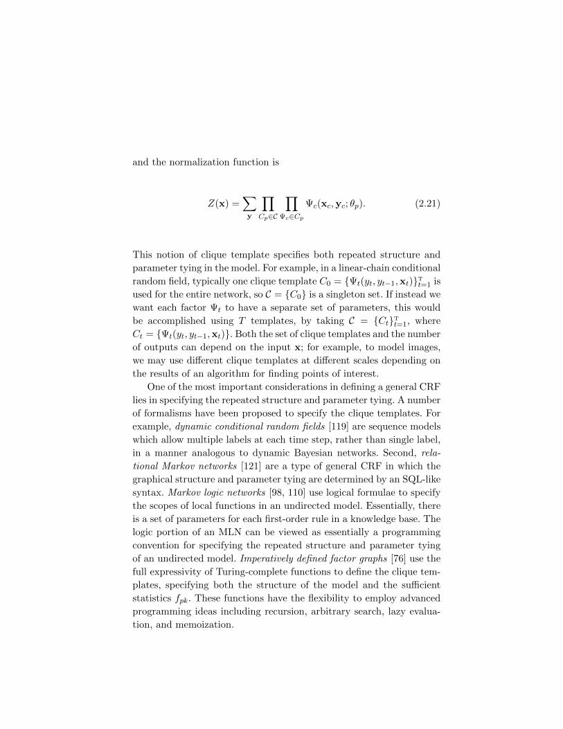
and the normalization function is

Z(x) =∑y

∏Cp∈C

∏Ψc∈Cp

Ψc(xc,yc; θp). (2.21)

This notion of clique template specifies both repeated structure and

parameter tying in the model. For example, in a linear-chain conditional

random field, typically one clique template C0 = {Ψt(yt, yt−1,xt)}Tt=1 is

used for the entire network, so C = {C0} is a singleton set. If instead we

want each factor Ψt to have a separate set of parameters, this would

be accomplished using T templates, by taking C = {Ct}Tt=1, where

Ct = {Ψt(yt, yt−1,xt)}. Both the set of clique templates and the number

of outputs can depend on the input x; for example, to model images,

we may use different clique templates at different scales depending on

the results of an algorithm for finding points of interest.

One of the most important considerations in defining a general CRF

lies in specifying the repeated structure and parameter tying. A number

of formalisms have been proposed to specify the clique templates. For

example, dynamic conditional random fields [119] are sequence models

which allow multiple labels at each time step, rather than single label,

in a manner analogous to dynamic Bayesian networks. Second, rela-

tional Markov networks [121] are a type of general CRF in which the

graphical structure and parameter tying are determined by an SQL-like

syntax. Markov logic networks [98, 110] use logical formulae to specify

the scopes of local functions in an undirected model. Essentially, there

is a set of parameters for each first-order rule in a knowledge base. The

logic portion of an MLN can be viewed as essentially a programming

convention for specifying the repeated structure and parameter tying

of an undirected model. Imperatively defined factor graphs [76] use the

full expressivity of Turing-complete functions to define the clique tem-

plates, specifying both the structure of the model and the sufficient

statistics fpk. These functions have the flexibility to employ advanced

programming ideas including recursion, arbitrary search, lazy evalua-

tion, and memoization.

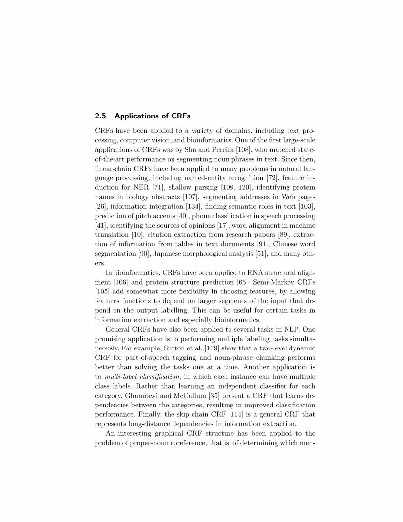
2.5 Applications of CRFs

CRFs have been applied to a variety of domains, including text pro-

cessing, computer vision, and bioinformatics. One of the first large-scale

applications of CRFs was by Sha and Pereira [108], who matched state-

of-the-art performance on segmenting noun phrases in text. Since then,

linear-chain CRFs have been applied to many problems in natural lan-

guage processing, including named-entity recognition [72], feature in-

duction for NER [71], shallow parsing [108, 120], identifying protein

names in biology abstracts [107], segmenting addresses in Web pages

[26], information integration [134], finding semantic roles in text [103],

prediction of pitch accents [40], phone classification in speech processing

[41], identifying the sources of opinions [17], word alignment in machine

translation [10], citation extraction from research papers [89], extrac-

tion of information from tables in text documents [91], Chinese word

segmentation [90], Japanese morphological analysis [51], and many oth-

ers.

In bioinformatics, CRFs have been applied to RNA structural align-

ment [106] and protein structure prediction [65]. Semi-Markov CRFs

[105] add somewhat more flexibility in choosing features, by allowing

features functions to depend on larger segments of the input that de-

pend on the output labelling. This can be useful for certain tasks in

information extraction and especially bioinformatics.

General CRFs have also been applied to several tasks in NLP. One

promising application is to performing multiple labeling tasks simulta-

neously. For example, Sutton et al. [119] show that a two-level dynamic

CRF for part-of-speech tagging and noun-phrase chunking performs

better than solving the tasks one at a time. Another application is

to multi-label classification, in which each instance can have multiple

class labels. Rather than learning an independent classifier for each

category, Ghamrawi and McCallum [35] present a CRF that learns de-

pendencies between the categories, resulting in improved classification

performance. Finally, the skip-chain CRF [114] is a general CRF that

represents long-distance dependencies in information extraction.

An interesting graphical CRF structure has been applied to the

problem of proper-noun coreference, that is, of determining which men-

tions in a document, such as Mr. President and he, refer to the same

underlying entity. McCallum and Wellner [73] learn a distance metric

between mentions using a fully-connected conditional random field in

which inference corresponds to graph partitioning. A similar model has

been used to segment handwritten characters and diagrams [22, 93].

In computer vision, several authors have used grid-shaped CRFs [43,

53] for labeling and segmenting images. Also, for recognizing objects,

Quattoni et al. [95] use a tree-shaped CRF in which latent variables

are designed to recognize characteristic parts of an object.

In some applications of CRFs, efficient dynamic programs exist even

though the graphical model is difficult to specify. For example, McCal-

lum et al. [75] learn the parameters of a string-edit model in order to

discriminate between matching and nonmatching pairs of strings. Also,

there is work on using CRFs to learn distributions over the derivations

of a grammar [99, 19, 127, 31].

2.6 Feature Engineering

In this section we describe some “tricks of the trade” that involve fea-

ture engineering. Although these apply especially to language applica-

tions, they are also useful more generally.

First, when the predicted variables are discrete, the features fpk of

a clique template Cp are ordinarily chosen to have a particular form:

fpk(yc,xc) = 1{yc=yc}qpk(xc). (2.22)

In other words, each feature is nonzero only for a single output config-

uration yc, but as long as that constraint is met, then the feature value

depends only on the input observation. Essentially, this means that we

can think of our features as depending only on the input xc, but that

we have a separate set of weights for each output configuration. This

feature representation is also computationally efficient, because com-

puting each qpk may involve nontrivial text or image processing, and

it need be evaluated only once for every feature that uses it. To avoid

confusion, we refer to the functions qpk(xc) as observation functions

rather than as features. Examples of observation functions are “word

xt is capitalized” and “word xt ends in ing”.

This representation can lead to a large number of features, which

can have significant memory and time requirements. For example, to

match state-of-the-art results on a standard natural language task, Sha

and Pereira [108] use 3.8 million features. Many of these features always

zero in the training data. In particular, some observation functions qpkare nonzero for certain output configurations and zero for others. This

point can be confusing: One might think that such features can have

no effect on the likelihood, but actually putting a negative weight on

them causes an assignment that does not appear in the training data

to become less likely, which improves the likelihood. For this reason,

including unsupported features typically results in better accuracy. In

order to save memory, however, sometimes these unsupported features,

that is, those which never occur in the training data, are removed from

the model.

As a simple heuristic for getting some of the benefits of unsupported

features with less memory, we have had success with an ad hoc tech-

nique for selecting a small set of unsupported features. The idea is to

add unsupported features only for likely paths, as follows: first train a

CRF without any unsupported features, stopping after a few iterations;

then add unsupported features fpk(yc,xc) for cases where xc occurs in

the training data for some instance x(i), and p(yc|x(i)) > ε.

McCallum [71] presents a more principled method of feature induc-

tion for CRFs, in which the model begins with a number of base fea-

tures, and the training procedure adds conjunctions of those features.

Alternatively, one can use feature selection. A modern method for fea-

ture selection is L1 regularization, which we discuss in Section 4.1.1.

Lavergne et al. [56] find that in the most favorable cases L1 finds models

in which only 1% of the full feature set is non-zero, but with compa-

rable performance to a dense feature setting. They also find it useful,

after optimizing the L1-regularized likelihood to find a set of nonzero

features, to fine-tune the weights of the nonzero features only using an

L2-regularized objective.

Second, if the observations are categorical rather than ordinal, that

is, if they are discrete but have no intrinsic order, it is important to

convert them to binary features. For example, it makes sense to learn

a linear weight on fk(y, xt) when fk is 1 if xt is the word dog and

0 otherwise, but not when fk is the integer index of word xt in the

text’s vocabulary. Thus, in text applications, CRF features are typically

binary; in other application areas, such as vision and speech, they are

more commonly real-valued. For real-valued features, it can help to

apply standard tricks such as normalizing the features to have mean

0 and standard deviation 1 or to bin the features to convert them to

categorical values.

Third, in language applications, it is sometimes helpful to include

redundant factors in the model. For example, in a linear-chain CRF,

one may choose to include both edge factors Ψt(yt, yt−1,xt) and vari-

able factors Ψt(yt,xt). Although one could define the same family of

distributions using only edge factors, the redundant node factors pro-

vide a kind of backoff, which is useful when the amount of data is

small compared to the number of features. (When there are hundreds

of thousands of features, many data sets are small!) It is important to

use regularization (Section 4.1.1) when using redundant features be-

cause it is the penalty on large weights that encourages the weight to

be spread across the overlapping features.

2.7 Notes on Terminology

Different parts of the theory of graphical models have been developed

independently in many different areas, so many of the concepts in this

chapter have different names in different areas. For example, undirected

models are commonly also referred to Markov random fields, Markov

networks, and Gibbs distributions. As mentioned, we reserve the term

“graphical model” for a family of distributions defined by a graph struc-

ture; “random field” or “distribution” for a single probability distribu-

tion; and “network” as a term for the graph structure itself. This choice

of terminology is not always consistent in the literature, partly because

it is not ordinarily necessary to be precise in separating these concepts.

Similarly, directed graphical models are commonly known as

Bayesian networks, but we have avoided this term because of its con-

fusion with the area of Bayesian statistics. The term generative model

is an important one that is commonly used in the literature, but is not

usually given a precise definition.

3

Inference

Efficient inference is critical for CRFs, both during training and for pre-

dicting the labels on new inputs. The are two inference problems that

arise. First, after we have trained the model, we often predict the labels

of a new input x using the most likely labeling y∗ = arg maxy p(y|x).

Second, as will be seen in Chapter 4, estimation of the parameters typ-

ically requires that we compute the marginal distribution for each edge

p(yt, yt−1|x), and also the normalizing function Z(x).

These two inference problems can be seen as fundamentally the

same operation on two different semirings [1], that is, to change the

marginalization problem to the maximization problem, we simply sub-

stitute max for plus. Although for discrete variables the marginals can

be computed by brute-force summation, the time required to do this

is exponential in the size of Y . Indeed, both inference problems are

intractable for general graphs, because any propositional satisfiability

problem can be easily represented as a factor graph.

In the case of linear-chain CRFs, both inference tasks can be per-

formed efficiently and exactly by variants of the standard dynamic-

programming algorithms for HMMs. We begin by presenting these

algorithms—the forward-backward algorithm for computing marginal

27

distributions and Viterbi algorithm for computing the most probable

assignment—in Section 3.1. These algorithms are a special case of the

more general belief propagation algorithm for tree-structured graphical

models (Section 3.2.2). For more complex models, approximate infer-

ence is necessary. In principle, we could run any approximate inference

algorithm we want, and substitute the resulting approximate marginals

for the exact marginals within the gradient (4.9). This can cause issues,

however, because for many optimization procedures, such as BFGS, we

require an approximation to the likelihood function as well. We discuss

this issue in Section 4.4.

In one sense, the inference problem for a CRF is no different than

that for any graphical model, so any inference algorithm for graphical

models can be used, as described in several textbooks [67, 49]. How-

ever, there are two additional issues that need to be kept in mind in

the context of CRFs. The first issue is that the inference subroutine is

called repeatedly during parameter estimation (Section 4.1.1 explains

why), which can be computationally expensive, so we may wish to trade

off inference accuracy for computational efficiency. The second issue is

that when approximate inference is used, there can be complex inter-

actions between the inference procedure and the parameter estimation

procedure. We postpone discussion of these issues to Chapter 4, when

we discuss parameter estimation, but it is worth mentioning them here

because they strongly influence the choice of inference algorithm.

3.1 Linear-Chain CRFs

In this section, we briefly review the inference algorithms for HMMs,

the forward-backward and Viterbi algorithms, and describe how they

can be applied to linear-chain CRFs. These standard inference algo-

rithms are described in more detail by Rabiner [96]. Both of these al-

gorithms are special cases of the belief propagation algorithm described

in Section 3.2.2, but we discuss the special case of linear chains in detail

both because it may help to make the earlier discussion more concrete,

and because it is useful in practice.

First, we introduce notation which will simplify the forward-

backward recursions. An HMM can be viewed as a factor graph

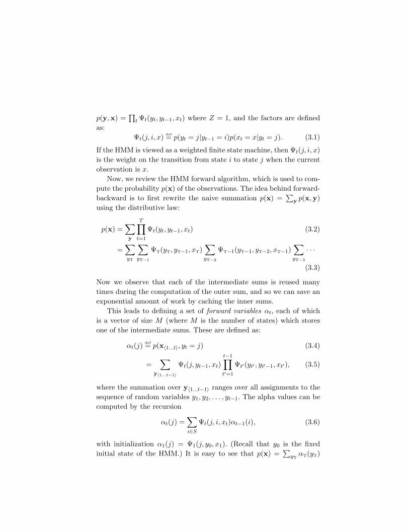
p(y,x) =∏t Ψt(yt, yt−1, xt) where Z = 1, and the factors are defined

as:

Ψt(j, i, x)def= p(yt = j|yt−1 = i)p(xt = x|yt = j). (3.1)

If the HMM is viewed as a weighted finite state machine, then Ψt(j, i, x)

is the weight on the transition from state i to state j when the current

observation is x.

Now, we review the HMM forward algorithm, which is used to com-

pute the probability p(x) of the observations. The idea behind forward-

backward is to first rewrite the naive summation p(x) =∑

y p(x,y)

using the distributive law:

p(x) =∑y

T∏t=1

Ψt(yt, yt−1, xt) (3.2)

=∑yT

∑yT−1

ΨT(yT, yT−1, xT)∑yT−2

ΨT−1(yT−1, yT−2, xT−1)∑yT−3

· · ·

(3.3)

Now we observe that each of the intermediate sums is reused many

times during the computation of the outer sum, and so we can save an

exponential amount of work by caching the inner sums.

This leads to defining a set of forward variables αt, each of which

is a vector of size M (where M is the number of states) which stores

one of the intermediate sums. These are defined as:

αt(j)def= p(x〈1...t〉, yt = j) (3.4)

=∑

y〈1...t−1〉

Ψt(j, yt−1, xt)t−1∏t′=1

Ψt′(yt′ , yt′−1, xt′), (3.5)

where the summation over y〈1...t−1〉 ranges over all assignments to the

sequence of random variables y1, y2, . . . , yt−1. The alpha values can be

computed by the recursion

αt(j) =∑i∈S

Ψt(j, i, xt)αt−1(i), (3.6)

with initialization α1(j) = Ψ1(j, y0, x1). (Recall that y0 is the fixed

initial state of the HMM.) It is easy to see that p(x) =∑

yTαT(yT)

by repeatedly substituting the recursion (3.6) to obtain (3.3). A formal

proof would use induction.

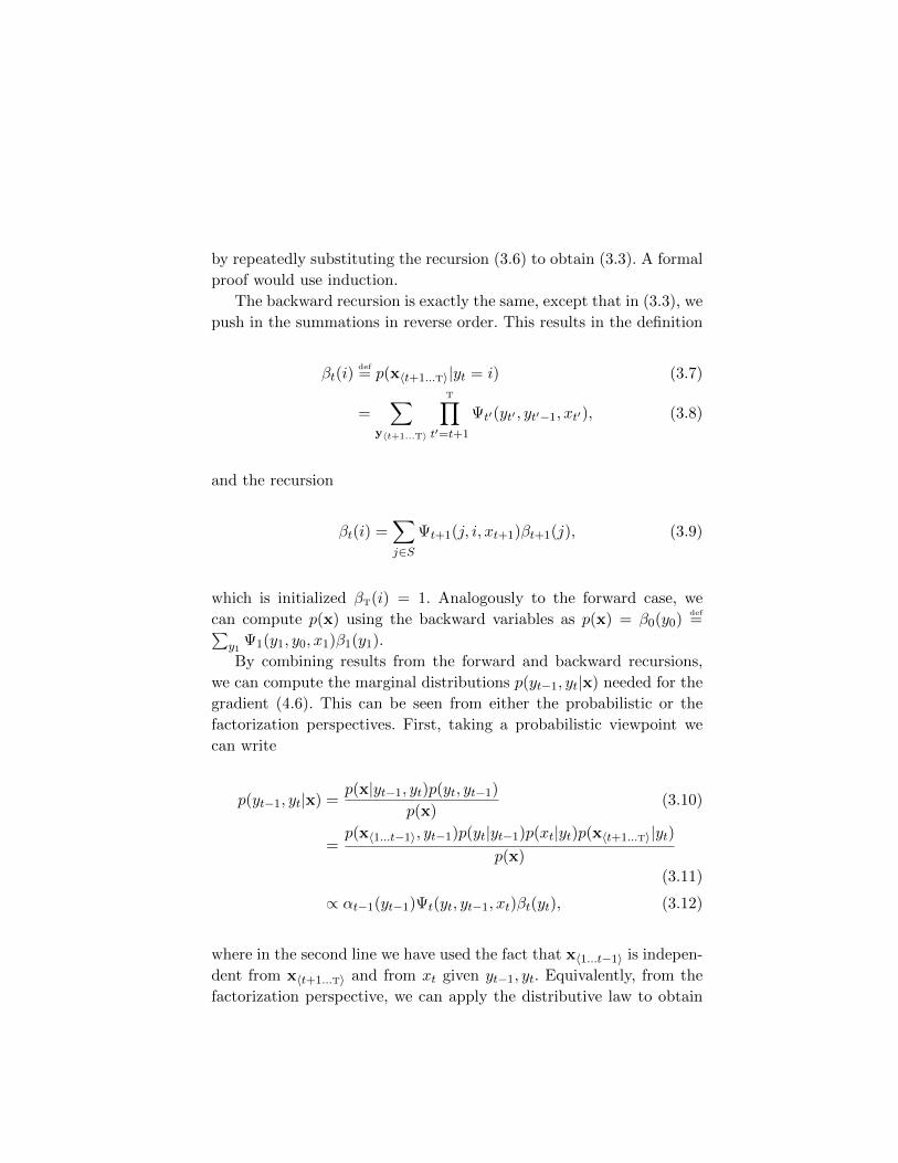
The backward recursion is exactly the same, except that in (3.3), we

push in the summations in reverse order. This results in the definition

βt(i)def= p(x〈t+1...T〉|yt = i) (3.7)

=∑

y〈t+1...T〉

T∏t′=t+1

Ψt′(yt′ , yt′−1, xt′), (3.8)

and the recursion

βt(i) =∑j∈S

Ψt+1(j, i, xt+1)βt+1(j), (3.9)

which is initialized βT(i) = 1. Analogously to the forward case, we

can compute p(x) using the backward variables as p(x) = β0(y0)def=∑

y1Ψ1(y1, y0, x1)β1(y1).

By combining results from the forward and backward recursions,

we can compute the marginal distributions p(yt−1, yt|x) needed for the

gradient (4.6). This can be seen from either the probabilistic or the

factorization perspectives. First, taking a probabilistic viewpoint we

can write

p(yt−1, yt|x) =p(x|yt−1, yt)p(yt, yt−1)

p(x)(3.10)

=p(x〈1...t−1〉, yt−1)p(yt|yt−1)p(xt|yt)p(x〈t+1...T〉|yt)

p(x)

(3.11)

∝ αt−1(yt−1)Ψt(yt, yt−1, xt)βt(yt), (3.12)

where in the second line we have used the fact that x〈1...t−1〉 is indepen-

dent from x〈t+1...T〉 and from xt given yt−1, yt. Equivalently, from the

factorization perspective, we can apply the distributive law to obtain

we see that

p(yt−1, yt,x) = Ψt(yt, yt−1, xt) ∑y〈1...t−2〉

t−1∏t′=1

Ψt′(yt′ , yt′−1, xt′)

∑

y〈t+1...T〉

T∏t′=t+1

Ψt′(yt′ , yt′−1, xt′)

, (3.13)

which can be computed from the forward and backward recursions as

p(yt−1, yt,x) = αt−1(yt−1)Ψt(yt, yt−1, xt)βt(yt). (3.14)

Once we have p(yt−1, yt,x), we can renormalize over yt, yt−1 to obtain

the desired marginal p(yt−1, yt|x).

Finally, to compute the globally most probable assignment y∗ =

arg maxy p(y|x), we observe that the trick in (3.3) still works if all

the summations are replaced by maximization. This yields the Viterbi

recursion:

δt(j) = maxi∈S

Ψt(j, i, xt)δt−1(i) (3.15)

Now that we have described the forward-backward and Viterbi

algorithms for HMMs, the generalization to linear-chain CRFs is

fairly straightforward. The forward-backward algorithm for linear-chain

CRFs is identical to the HMM version, except that the transition

weights Ψt(j, i, xt) are defined differently. We observe that the CRF

model (2.16) can be rewritten as:

p(y|x) =1

Z(x)

T∏t=1

Ψt(yt, yt−1,xt), (3.16)

where we define

Ψt(yt, yt−1,xt) = exp

{∑k

θkfk(yt, yt−1,xt)

}. (3.17)

With that definition, the forward recursion (3.6), the backward re-

cursion (3.9), and the Viterbi recursion (3.15) can be used unchanged

for linear-chain CRFs. Instead of computing p(x) as in an HMM, in a

CRF the forward and backward recursions compute Z(x).

We mention three more specialised inference tasks that can also be

solved using direct analogues of the HMM algorithms. First, assign-

ments to y can be sampled from the joint posterior p(y|x) using the

forward algorithm combined with a backward sampling place, in exactly

the same way as an HMM. Second, if instead of finding the single best

assignment arg maxy p(y|x), we wish to find the k assignments with

highest probability, we can do this also using the standard algorithms

from HMMs. Finally, sometimes it is useful to compute a marginal prob-

ability p(yt, yt+1, . . . yt+k|x) over a possibly non-contiguous range of

nodes. For example, this is useful for measuring the model’s confidence

in its predicted labeling over a segment of input. This marginal proba-

bility can be computed efficiently using constrained forward-backward,

as described by Culotta and McCallum [25].

3.2 Inference in Graphical Models

Exact inference algorithms for general graphs exist. Although these al-

gorithms require exponential time in the worst case, they can still be

efficient for graphs that occur in practice. The most popular exact algo-

rithm, the junction tree algorithm, successively clusters variables until

the graph becomes a tree. Once an equivalent tree has been constructed,

its marginals can be computed using exact inference algorithms that

are specific to trees. However, for certain complex graphs, the junction

tree algorithm is forced to make clusters which are very large, which

is why the procedure still requires exponential time in the worst case.

For more details on exact inference, see Koller and Friedman [49].

For this reason, an enormous amount of effort has been devoted to

approximate inference algorithms. Two classes of approximate inference

algorithms have received the most attention: Monte Carlo algorithms

and variational algorithms. Monte Carlo algorithms are stochastic al-

gorithms that attempt to approximately produce a sample from the

distribution of interest. Variational algorithms are algorithms that con-

vert the inference problem into an optimization problem, by attempting

to find a simple distribution that most closely matches the intractable

distribution of interest. Generally, Monte Carlo algorithms are unbiased

in the sense that they guaranteed to sample from the distribution of

interest given enough computation time, although it is usually impos-

sible in practice to know when that point has been reached. Variational

algorithms, on the other hand, can be much faster, but they tend to

be biased, by which we mean that they tend to have a source of error

that is inherent to the approximation, and cannot be easily lessened

by giving them more computation time. Despite this, variational algo-

rithms can be useful for CRFs, because parameter estimation requires

performing inference many times, and so a fast inference procedure is

vital to efficient training.

In the remainder of this section, we outline two examples of ap-

proximate inference algorithms, one from each of these two categories.

Too much work has been done on approximate inference for us to at-

tempt to summarize it here. Rather, our aim is to highlight the general

issues that arise when using approximate inference algorithms within

CRF training. In this chapter, we focus on describing the inference al-

gorithms themselves, whereas in Chapter 4 we discuss their application

to CRFs.

3.2.1 Markov Chain Monte Carlo

Currently the most popular type of Monte Carlo method for complex

models is Markov Chain Monte Carlo (MCMC) [101]. Rather than

attempting to approximate a marginal distribution p(ys|x) directly,

MCMC methods generate approximate samples from the joint distri-

bution p(y|x). MCMC methods work by constructing a Markov chain,

whose state space is the same as that of Y , in careful way so that when

the chain is simulated for a long time, the distribution over states of

the chain is approximately p(ys|x). Suppose that we want to approxi-

mate the expectation of some function f(x,y) that depends on. Given

a sample y1,y2, . . . ,yM from a Markov chain in an MCMC method,

we can approximate this expectation as:

∑y

p(y|x)f(x,y) ≈ 1

M

M∑j=1

f(x,yj) (3.18)

For example, in the context of CRFs, these approximate expectations

can then be used to approximate the quantities required for learning,

specifically the gradient (4.6).

A simple example of an MCMC method is Gibbs sampling. In each

iteration of the Gibbs sampling algorithm, each variable is resampled

individually, keeping all of the other variables fixed. Suppose that we

already have a sample yj from iteration j. Then to generate the next

sample yj+1,

(1) Set yj+1 ← yj .

(2) For each s ∈ V , resample component s. Sample yj+1s from

the distribution p(ys|y\s,x).

(3) Return the resulting value of yj+1.

This procedure defines a Markov chain that can be used to approx-

imation expectations as in (3.18). In the case of general CRFs, then

using the notation from Section 2.4, this conditional probability can be

computed as

p(ys|y\s,x) = κ∏Cp∈C

∏Ψc∈Cp

Ψc(xc,yc; θp), (3.19)

where κ is a normalizing constant. This is much easier to compute than

the joint probability p(y|x), because computing κ requires a summation

only over all possible values of ys rather than assignments to the full

vector y.

A major advantage of Gibbs sampling is that it is simple to imple-

ment. Indeed, software packages such as BUGS can take a graphical

model as input and automatically compile an appropriate Gibbs sam-

pler [66]. The main disadvantage of Gibbs sampling is that it can work

poorly if p(y|x) has strong dependencies, which is often the case in

sequential data. By “works poorly” we mean that it may take many

iterations before the distribution over samples from the Markov chain

is close to the desired distribution p(y|x).

There is an enormous literature on MCMC algorithms. The text-

book by Robert and Casella [101] provides an overview. However,

MCMC algorithms are not commonly applied in the context of con-

ditional random fields. Perhaps the main reason for this is that as we

have mentioned earlier, parameter estimation by maximum likelihood

requires calculating marginals many times. In the most straightforward

approach, one MCMC chain would be run for each training example

for each parameter setting that is visited in the course of a gradient de-

scent algorithm. Since MCMC chains can take thousands of iterations

to converge, this can be computationally prohibitive. One can imagine

ways of addressing this, such as not running the chain all the way to

convergence (see Section 4.4.3).

3.2.2 Belief Propagation

An important variational inference algorithm is belief propagation

(BP), which we explain in this section. In addition, it is a direct gen-

eralization of the exact inference algorithms for linear-chain CRFs.

Suppose that G is a tree, and we wish to compute the marginal

distribution of a variable s. The intuition behind BP is that each of

the neighboring factors of s makes a multiplicative contribution to the

marginal of s, called a message, and each of these messages can be

computed separately because the graph is a tree. More formally, for

every factor a ∈ N(s), call Va the set of variables that are “upstream”

of a, that is, the set of variables v for which a is between s and v.

In a similar fashion, call Fa the set of factors that are upstream of a,

including a itself. But now because G is a tree, the sets {Va} ∪ {s}form a partition of the variables in G. This means that we can split up

the summation required for the marginal into a product of independent

subproblems as:

p(ys) ∝∑y\ys

∏a

Ψa(ya) (3.20)

=∏

a∈N(s)

∑yVa

∏Ψb∈Fa

Ψb(yb) (3.21)

Denote each factor in the above equation by mas, that is,

mas(xs) =∑yVa

∏Ψb∈Fa

Ψb(yb), (3.22)

can be thought of as a message from the factor a to the variable s that

summarizes the impact of the network upstream of a on the belief in s.

In a similar fashion, we can define messages from variables to factors

as

msA(xs) =∑yVs

∏Ψb∈Fs

Ψb(yb). (3.23)

Then, from (3.21), we have that the marginal p(ys) is proportional to

the product of all the incoming messages to variable s. Similarly, factor

marginals can be computed as

p(ya) ∝ Ψa(ya)∏s∈a

msa(ya). (3.24)

Here we treat a as a set a variables denoting the scope of factor Ψa,

as we will throughout. In addition, we will sometimes use the reverse

notation c 3 s to mean the set of all factors c that contain the variable

s.

Naively computing the messages according to (3.22) is impractical,

because the messages as we have defined them require summation over

possibly many variables in the graph. Fortunately, the messages can

also be written using a recursion that requires only local summation.

The recursion is

mas(xs) =∑ya\ys

Ψa(ya)∏t∈a\s

mta(xt)

msa(xs) =∏

b∈N(s)\a

mbs(xs)(3.25)

That this recursion matches the explicit definition of m can be seen by

repeated substitution, and proven by induction. In a tree, it is possible

to schedule these recursions such that the antecedent messages are

always sent before their dependents, by first sending messages from

the root, and so on. This is the algorithm known as belief propagation

[88].

In addition to computing single-variable marginals, we will also wish

to compute factor marginals p(ya) and joint probabilites p(y) for a

given assignment y. (Recall that the latter problem is difficult because

it requires computing the partition function logZ.) First, to compute

marginals over factors—or over any connected set of variables, in fact—

we can use the same decomposition of the marginal as for the single-

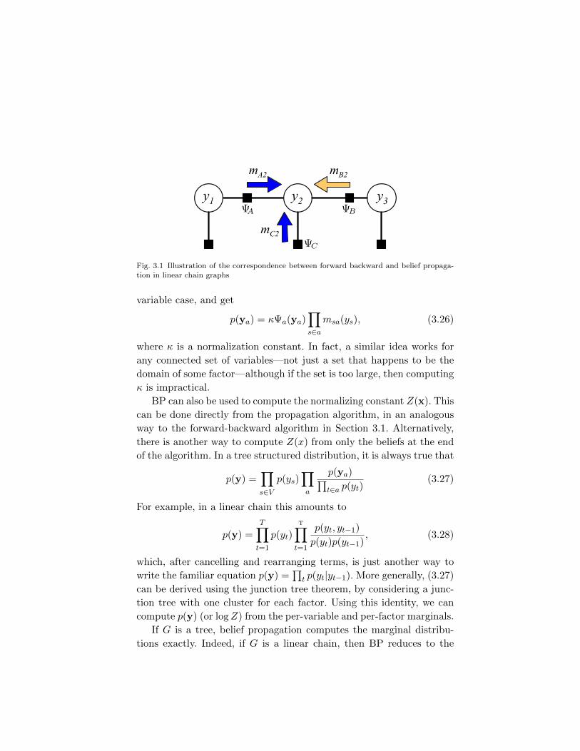
y1 y2 y3ΨA ΨB

mA2 mB2

mC2ΨC

Fig. 3.1 Illustration of the correspondence between forward backward and belief propaga-tion in linear chain graphs

variable case, and get

p(ya) = κΨa(ya)∏s∈a

msa(ys), (3.26)

where κ is a normalization constant. In fact, a similar idea works for

any connected set of variables—not just a set that happens to be the

domain of some factor—although if the set is too large, then computing

κ is impractical.

BP can also be used to compute the normalizing constant Z(x). This

can be done directly from the propagation algorithm, in an analogous

way to the forward-backward algorithm in Section 3.1. Alternatively,

there is another way to compute Z(x) from only the beliefs at the end

of the algorithm. In a tree structured distribution, it is always true that

p(y) =∏s∈V

p(ys)∏a

p(ya)∏t∈a p(yt)

(3.27)

For example, in a linear chain this amounts to

p(y) =T∏t=1

p(yt)T∏t=1

p(yt, yt−1)

p(yt)p(yt−1), (3.28)

which, after cancelling and rearranging terms, is just another way to

write the familiar equation p(y) =∏t p(yt|yt−1). More generally, (3.27)

can be derived using the junction tree theorem, by considering a junc-

tion tree with one cluster for each factor. Using this identity, we can

compute p(y) (or logZ) from the per-variable and per-factor marginals.

If G is a tree, belief propagation computes the marginal distribu-

tions exactly. Indeed, if G is a linear chain, then BP reduces to the

forward-backward algorithm (Section 3.1). To see this, refer to Fig-

ure 3.1. The figure shows a three node linear chain along with the BP

messages as we have described them in this section. To see the corre-

spondence to forward backward, the forward message that we denoted

α2 in Section 3.1 corresponds to the product of the two messages mA2

and mC2 (the thick, dark blue arrows in the figure). The backward

message β2 corresponds to the message mB2 (the thick, light orange

arrow in the figure).

If G is not a tree, the message updates (3.25) are no longer guar-

anteed to return the exact marginals, nor are they guaranteed even to

converge, but we can still iterate them in an attempt to find a fixed

point. This procedure is called loopy belief propagation. To emphasize

the approximate nature of this procedure, we refer to the approximate

marginals that result from loopy BP as beliefs rather than as marginals,

and denote them by q(ys).

Surprisingly, loopy BP can be seen as a variational method for in-

ference, meaning that there actually exists an objective function over

beliefs that is approximately minimized by the iterative BP procedure.

Several introductory papers [137, 131] describe this in more detail.

The general idea behind a variational algorithm is:

(1) Define a family of tractable distributions Q and an objective

functionO(q). The functionO should be designed to measure

how well a tractable distribution q ∈ Q approximates the

distribution p of interest.

(2) Find the “closest” tractable distribution q∗ = minq∈QO(q).

(3) Use the marginals of q∗ to approximate those of p.

For example, suppose that we take Q be the set of all possible distri-

butions over y, and we choose the objective function

O(q) = KL(q‖p)− logZ (3.29)

= −H(q)−∑a

q(ya) log Ψa(ya). (3.30)

Then the solution to this variational problem is q∗ = p with optimal

value O(q∗) = logZ. Solving this particular variational formulation is

thus equivalent to performing exact inference. Approximate inference

techniques can be devised by changing the set Q—for example, by

requiring q to be fully factorized—or by using a different objective O.

For example, the mean field method arises by requiring q to be fully

factorized, i.e., q(y) =∏s qs(ys) for some choice for qs, and finding the

factorized q that most closely matches p.

With that background on variational methods, let us see how belief

propagation can be understood in this framework. We make two ap-

proximations. First, we approximate the entropy term H(q) of (3.30),

which as it stands is difficult to compute. If q were a tree-structured

distribution, then its entropy could be written exactly as

HBethe(q) =∑a

q(ya) log q(ya) +∑i

(1− di)q(yi) log q(yi). (3.31)

This follows from substituting the junction-tree formulation (3.27) of

the joint into the definition of entropy. If q is not a tree, then we can still

take HBethe as an approximation to H to compute the exact variational

objective O. This yields the Bethe free energy :

OBethe(q) = HBethe(q)−∑a

q(ya) log Ψa(ya) (3.32)

The objective OBethe depends on q only through its marginals, so rather

than optimizing it over all probability distributions q, we can optimize

over the space of all marginal vectors. Specifically, every distribution q

has an associated belief vector q, with elements qa;ya for each factor a

and assignment ya, and elements qi;yi for each variable i and assignment

yi. The space of all possible belief vectors has been called the marginal

polytope [130]. However, for intractable models, the marginal polytope

can have extremely complex structure.

This leads us to the second variational approximation made by loopy

BP, namely that the objective OBethe is optimized instead over a relax-

ation of the marginal polytope. The relaxation is to require that the

beliefs be only locally consistent, that is, that∑ya\yi

qa(ya) = qi(yi) ∀a, i ∈ a (3.33)

Under these constraints, Yedidia et al. [136] show that constrained

stationary points of OBethe fixed points of loopy BP. So we can view

the Bethe energy OBethe as an objective function that the loopy BP

fixed-point operations attempt to optimize.

This variational perspective provides new insight into the method

that would not be available if we thought of it solely from the mes-

sage passing perspective. One of the most important insights is that

it shows how to use loopy BP to approximate logZ. Because we in-

troduced minqOBethe(q) as an approximation to minqO(q), and we

know that minqO(q) = logZ, then it seems reasonable to define

logZBethe = minqOBethe(q) as an approximation to logZ. This will be

important when we discuss CRF parameter estimation using BP in

Section 4.4.2.

3.3 Implementation Concerns

In this section, we mention a few implementation techniques that are

important to practical inference in CRFs: sparsity and preventing nu-

merical underflow.

First, it is often possible to exploit sparsity in the model to make

inference more efficient. Two different types of sparsity are relevant:

sparsity in the factor values, and sparsity in the features. First, about

the factor values, recall that in the linear-chain case, each of the for-

ward updates (3.6) and backward updates (3.9) requires O(M2) time,

that is, quadratic time in the number of labels. Analogously, in general

CRFs, an update of loopy BP in a model with pairwise factors requires

O(M2) time. In some models, however, it is possible to implement in-

ference more efficiently, because it is known a priori not all factor values

(yt, yt−1) are feasible, that is, the factor Ψt(yt, yt+1,xt) is 0 for many

values yt, yt+1. In such cases, the computational cost of sending a mes-

sage can be reduced by implementing the message-passing iterations

using sparse matrix operations.

The second kind of sparsity that is useful is sparsity in the feature

vectors. Recall from (2.20) that computing the factors Ψc(xc,yc) re-

quires computing a dot product between the parameter vector θp and

and the vector of features Fc = {fpk(yc,xc)}. Often, many elements

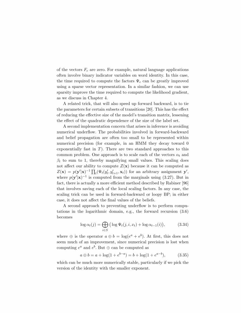
of the vectors Fc are zero. For example, natural language applications

often involve binary indicator variables on word identity. In this case,

the time required to compute the factors Ψc can be greatly improved

using a sparse vector representation. In a similar fashion, we can use

sparsity improve the time required to compute the likelihood gradient,

as we discuss in Chapter 4.

A related trick, that will also speed up forward backward, is to tie

the parameters for certain subsets of transitions [20]. This has the effect

of reducing the effective size of the model’s transition matrix, lessening

the effect of the quadratic dependence of the size of the label set.

A second implementation concern that arises in inference is avoiding

numerical underflow. The probabilities involved in forward-backward

and belief propagation are often too small to be represented within

numerical precision (for example, in an HMM they decay toward 0

exponentially fast in T ). There are two standard approaches to this

common problem. One approach is to scale each of the vectors αt and

βt to sum to 1, thereby magnifying small values. This scaling does

not affect our ability to compute Z(x) because it can be computed as

Z(x) = p(y′|x)−1∏t(Ψt(y

′t, y′t+1,xt)) for an arbitrary assignment y′,

where p(y′|x)−1 is computed from the marginals using (3.27). But in

fact, there is actually a more efficient method described by Rabiner [96]

that involves saving each of the local scaling factors. In any case, the

scaling trick can be used in forward-backward or loopy BP; in either

case, it does not affect the final values of the beliefs.

A second approach to preventing underflow is to perform compu-

tations in the logarithmic domain, e.g., the forward recursion (3.6)

becomes

logαt(j) =⊕i∈S

(log Ψt(j, i, xt) + logαt−1(i)

), (3.34)

where ⊕ is the operator a ⊕ b = log(ea + eb). At first, this does not

seem much of an improvement, since numerical precision is lost when

computing ea and eb. But ⊕ can be computed as

a⊕ b = a+ log(1 + eb−a) = b+ log(1 + ea−b), (3.35)

which can be much more numerically stable, particularly if we pick the

version of the identity with the smaller exponent.

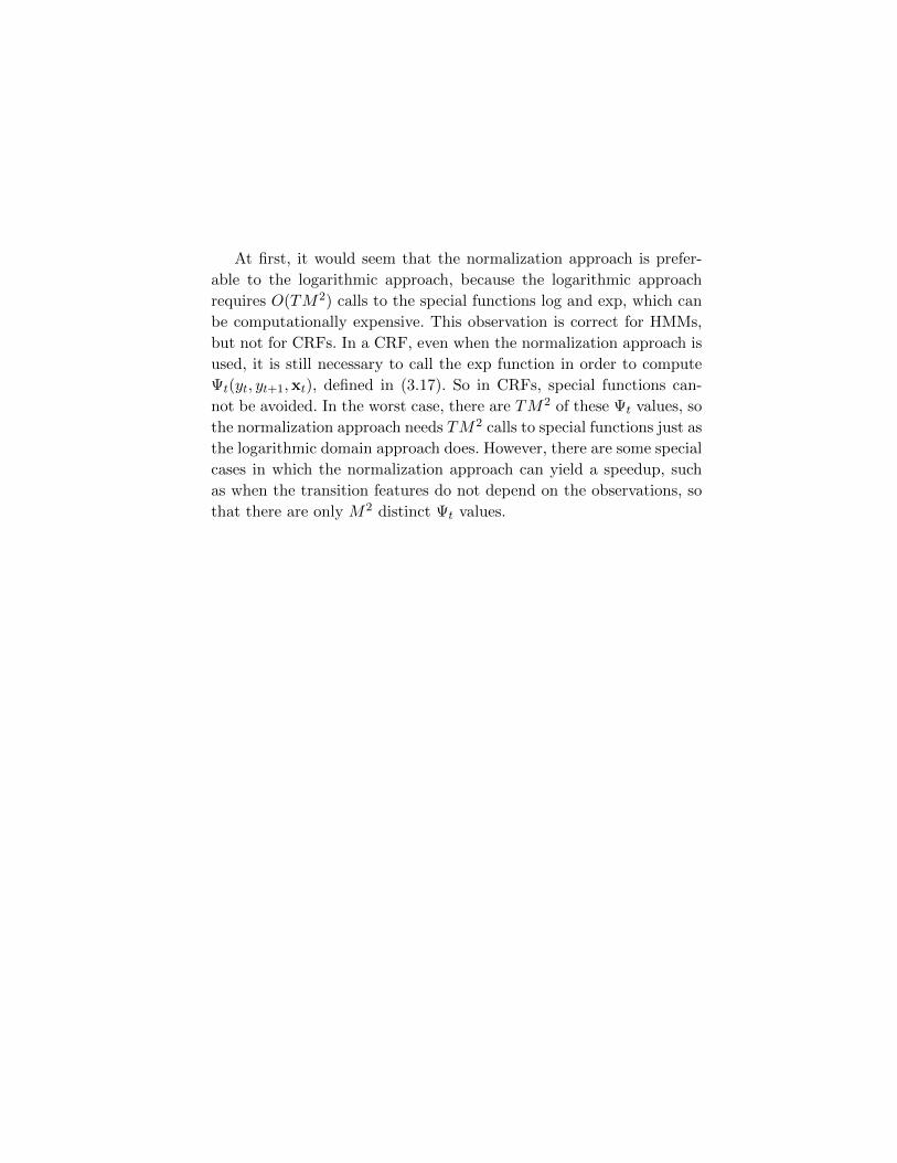
At first, it would seem that the normalization approach is prefer-

able to the logarithmic approach, because the logarithmic approach

requires O(TM2) calls to the special functions log and exp, which can

be computationally expensive. This observation is correct for HMMs,

but not for CRFs. In a CRF, even when the normalization approach is

used, it is still necessary to call the exp function in order to compute

Ψt(yt, yt+1,xt), defined in (3.17). So in CRFs, special functions can-

not be avoided. In the worst case, there are TM2 of these Ψt values, so

the normalization approach needs TM2 calls to special functions just as

the logarithmic domain approach does. However, there are some special

cases in which the normalization approach can yield a speedup, such

as when the transition features do not depend on the observations, so

that there are only M2 distinct Ψt values.

4

Parameter Estimation

In this chapter we discuss how to estimate the parameters θ = {θk}of a conditional random field. In the simplest and typical case, we are

provided with fully labeled independent data, but there has also been

work in CRFs with latent variables and CRFs for relational learning.

CRFs are trained by maximum likelihood, that is, the parameters

are chosen such that the training data has highest probability under

the model. In principle, this can be done in a manner exactly analogous

to logistic regression, which should not be surprising given the close re-

lationship between these models that was described in Chapter 2. The

main difference is computational: CRFs tend to have more parame-

ters and more complex structure than a simple classifier, so training is

correspondingly more expensive.

In tree structured CRFs, the maximum likelihood parameters can

be found by a numerical optimization procedure that calls the infer-

ence algorithms of Section 3.1 as a subroutine. Crucially, the likelihood

is a convex function of the parameters, which means that powerful

optimization procedures are available that provably converge to the

optimal solution. For general CRFs, on the other hand, maximum like-

lihood training is intractable. One way to deal with this problem is

43

to use approximate inference methods, as discussed in Chapter 3, but

another way is to choose a different training criterion than maximum

likelihood.

We begin by describing maximum likelihood training, both in the

linear chain case (Section 4.1.1) and in the case of general graphical

structures (Section 4.1.2), including the case of latent variables. Then

we discuss training in general graphical structures, in which approxima-

tions are necessary. We also describe two general methods for speed-

ing up parameter estimation that exploit iid structure in the data:

stochastic gradient descent (Section 4.2) and multithreaded training

(Section 4.3). In CRFs with general structure, typically approximate

inference procedures must be used. The approximate training proce-

dures build on the approximate algorithms for inference described in

Chapter 3, but there can be complications in the interaction between

approximate inference and learning. This is described in Section 4.4.

4.1 Maximum Likelihood

4.1.1 Linear-chain CRFs

In a linear-chain CRF, the maximum likelihood parameters can be

determined using numerical optimization methods. We are given iid

training data D = {x(i),y(i)}Ni=1, where each x(i) = {x(i)1 ,x

(i)2 , . . .x

(i)T }

is a sequence of inputs, and each y(i) = {y(i)1 , y

(i)2 , . . . y

(i)T } is a sequence

of the desired predictions.

Parameter estimation is typically performed by penalized maximum

likelihood. Because we are modeling the conditional distribution, the

following log likelihood, sometimes called the conditional log likelihood,

is appropriate:

`(θ) =N∑i=1

log p(y(i)|x(i)). (4.1)

One way to understand the conditional likelihood p(y|x; θ) is to imagine

combining it with some arbitrary prior p(x; θ′) to form a joint p(y,x).

Then when we optimize the joint log likelihood

log p(y,x) = log p(y|x; θ) + log p(x; θ′), (4.2)

the two terms on the right-hand side are decoupled, that is, the value of

θ′ does not affect the optimization over θ. If we do not need to estimate

p(x), then we can simply drop the second term, which leaves (4.1).

After substituting in the CRF model (2.16) into the likelihood (4.1),

we get the following expression:

`(θ) =

N∑i=1

T∑t=1

K∑k=1

θkfk(y(i)t , y

(i)t−1,x

(i)t )−

N∑i=1

logZ(x(i)), (4.3)

It is often the case that we have a large number of parameters, e.g.,

several hundred thousand. As a measure to avoid overfitting, we use

regularization, which is a penalty on weight vectors whose norm is too

large. A common choice of penalty is based on the Euclidean norm of θ

and on a regularization parameter 1/2σ2 that determines the strength

of the penalty. Then the regularized log likelihood is

`(θ) =

N∑i=1

T∑t=1

K∑k=1

θkfk(y(i)t , y

(i)t−1,x

(i)t )−

N∑i=1

logZ(x(i))−K∑k=1

θ2k

2σ2. (4.4)

The parameter σ2 is a free parameter which determines how much to

penalize large weights. Intuitively, the idea is to reduce the potential

for a small number of features to dominate the prediction. The nota-

tion for the regularizer is intended to suggest that regularization can

also be viewed as performing maximum a posteriori (MAP) estima-

tion of θ, if θ is assigned a Gaussian prior with mean 0 and covari-

ance σ2I. Determining the best regularization parameter can require a

computationally-intensive parameter sweep. Fortunately, often the ac-

curacy of the final model is not sensitive to small changes in σ2 (e.g.,

up to a factor of 10). The best value of σ2 depends on the size of the

training set; for medium-sized training sets, σ2 = 10 is typical.

An alternative choice of regularization is to use the L1 norm instead

of the Euclidean norm, which corresponds to an exponential prior on

parameters [37]. This results in the following penalized likelihood:

`′(θ) =

N∑i=1

T∑t=1

K∑k=1

θkfk(y(i)t , y

(i)t−1,x

(i)t )−

N∑i=1

logZ(x(i))− αK∑k=1

|θk|.

(4.5)

This regularizer tends to encourage sparsity in the learned parameters,

meaning that most of the θk are 0. This can be useful for performing

feature selection, and also has theoretical advantages [84]. In practice,

models trained with the L1 regularizer tend to be sparser but have

roughly the same accuracy as models training using the L2 regularizer

[56]. A disadvantage of the L1 regularizer is that it is not differentiable

at 0, which complicates numerical parameter estimation somewhat [37,

3, 138].

In general, the function `(θ) cannot be maximized in closed form,

so numerical optimization is used. The partial derivatives of (4.4) are

∂`

∂θk=

N∑i=1

T∑t=1

fk(y(i)t , y

(i)t−1,x

(i)t )−

N∑i=1

T∑t=1

∑y,y′

fk(y, y′,x

(i)t )p(y, y′|x(i))− θk

σ2.

(4.6)

The first term is the expected value of fk under the empirical distribu-

tion:

p(y,x) =1

N

N∑i=1

1{y=y(i)}1{x=x(i)}. (4.7)

The second term, which arises from the derivative of logZ(x), is the

expectation of fk under the model distribution p(y|x; θ)p(x). Therefore,

at the unregularized maximum likelihood solution, when the gradient

is zero, these two expectations are equal. This pleasing interpretation is

a standard result about maximum likelihood estimation in exponential

families.

To compute the likelihood `(θ) and its derivative requires techniques

from inference in graphical models. In the likelihood, inference is needed

to compute the partition function Z(x(i)), which is a sum over all pos-

sible labellings. In the derivatives, inference is required to compute the

marginal distributions p(y, y′|x(i)). Because both of these quantities

depend on x(i), we will need to run inference once for each training

instance every time the likelihood is computed. This is the key compu-

tational difference between CRFs and generative Markov random fields.

In linear-chain models, inference can be performed efficiently using the

algorithms described in Section 3.1.

Now we discuss how to optimize `(θ). The function `(θ) is con-

cave, which follows from the convexity of functions of the form g(x) =

log∑

i expxi. Convexity is extremely helpful for parameter estimation,

because it means that every local optimum is also a global optimum.

Adding regularization ensures that ` is strictly concave, which implies

that it has exactly one global optimum.

Perhaps the simplest approach to optimize ` is steepest ascent along

the gradient (4.6), but this requires too many iterations to be practical.

Newton’s method converges much faster because it takes into account

the curvature of the likelihood, but it requires computing the Hessian,

the matrix of all second derivatives. The size of the Hessian is quadratic

in the number of parameters. Since practical applications often use tens

of thousands or even millions of parameters, simply storing the full

Hessian is not practical.

Instead, current techniques for optimizing (4.4) make approximate

use of second-order information. Particularly successful have been

quasi-Newton methods such as BFGS [6], which compute an approx-

imation to the Hessian from only the first derivative of the objective

function. A full K × K approximation to the Hessian still requires

quadratic size, however, so a limited-memory version of BFGS is used,

due to Byrd et al. [14]. Conjugate gradient is another optimization tech-

nique that also makes approximate use of second-order information and

has been used successfully with CRFs. For a good introduction to both

limited-memory BFGS and conjugate gradient, see Nocedal and Wright

[87]. Either can be thought of as a black-box optimization routine that

is a drop-in replacement for vanilla gradient ascent. When such second-

order methods are used, gradient-based optimization is much faster

than the original approaches based on iterative scaling in Lafferty et al.

[54], as shown experimentally by several authors [108, 132, 68, 79]. Fi-

nally, trust region methods have recently been shown to perform well

on multinomial logistic regression [63], and may work well for CRFs as

well.

Finally, we discuss the computational cost of training linear chain

models. As we will see in Section 3.1, the likelihood and gradient for

a single training instance can be computed by forward-backward in

time O(TM2), where M is the number of labels and T the length of

the training instance. Because we need to run forward-backward for

each training instance, each computation of the likelihood and gra-

dient requires O(TM2N) time, so that the total cost of training is

O(TM2NG), where G the number of gradient computations required

by the optimization procedure. Unfortunately, G depends on the data

set and is difficult to predict in advance. For batch L-BFGS on linear-

chain CRFs, it is often but not always under 100. For many data sets,

this cost is reasonable, but if the number of states M is large, or the

number of training sequences N is very large, then this can become

expensive. Depending on the number of labels, training CRFs can take

anywhere from a few minutes to a few days; see Section 4.5 for exam-

ples.

4.1.2 General CRFs

Parameter estimation for general CRFs is essentially the same as for

linear-chains, except that computing the model expectations requires

more general inference algorithms. First, we discuss the fully-observed

case, in which the training and testing data are independent, and the

training data is fully observed. In this case the conditional log likeli-

hood, using the notation of Section 2.4, is

`(θ) =∑Cp∈C

∑Ψc∈Cp

K(p)∑k=1

θpkfpk(xc,yc)− logZ(x). (4.8)

The equations in this section do not explicitly sum over training in-

stances, because if a particular application happens to have iid training

instances, they can be represented by disconnected components in the

graph G.

The partial derivative of the log likelihood with respect to a param-

eter θpk associated with a clique template Cp is

∂`

∂θpk=∑

Ψc∈Cp

fpk(xc,yc)−∑

Ψc∈Cp

∑y′c

fpk(xc,y′c)p(y

′c|x). (4.9)

The function `(θ) has many of the same properties as in the linear-chain

case. First, the zero-gradient conditions can be interpreted as requiring

that the sufficient statistics Fpk(x,y) =∑

Ψcfpk(xc,yc) have the same

expectations under the empirical distribution and under the model dis-

tribution. Second, the function `(θ) is concave, and can be efficiently

maximized by second-order techniques such as conjugate gradient and

L-BFGS. Finally, regularization is used just as in the linear-chain case.

All of the discussion so far has assumed that the training data con-

tains the true values of all the label variables in the model. In the latent

variable case, on the other hand, the model contains variables that are

observed at neither training nor test time. This situation is called a

hidden-state CRF (HCRF) by Quattoni et al. [95] which was one of

the first examples of latent variable CRFs. Quattoni et al. [94] present

a more detailed description. For other early applications of HCRFs,

see [120, 75]. It is more difficult to train CRFs with latent variables

because the latent variables need to be marginalized out to compute

the likelihood. Because of this difficultly, the original work on CRFs

focused on fully-observed training data, but recently there has been

increasing interest in HCRFs.

Suppose we have a conditional random field with inputs x in which

the output variables y are observed in the training data, but we have

additional variables w that are latent, so that the CRF has the form

p(y,w|x) =1

Z(x)

∏Cp∈C

∏Ψc∈Cp

Ψc(xc,wc,yc; θp). (4.10)

A natural objective function to maximize during training is the

marginal likelihood

`(θ) = log p(y|x) = log∑w

p(y,w|x). (4.11)

The first question is how even to compute the marginal likelihood `(θ),

because if there are many variables w, the sum cannot be computed di-

rectly. The key is to realize that we need to compute log∑

w p(y,w|x)

not for any possible assignment y, but only for the particular assign-

ment that occurs in the training data. This motivates taking the origi-

nal CRF (4.10), and clamping the variables Y to their observed values

in the training data, yielding a distribution over w:

p(w|y,x) =1

Z(y,x)

∏Cp∈C

∏Ψc∈Cp

Ψc(xc,wc,yc; θp), (4.12)

where the normalization factor is

Z(y,x) =∑w

∏Cp∈C

∏Ψc∈Cp

Ψc(xc,wc,yc; θp). (4.13)

This new normalization constant Z(y,x) can be computed by the same

inference algorithm that we use to compute Z(x). In fact, Z(y,x) is

easier to compute, because it sums only over w, while Z(x) sums over

both w and y. Graphically, this amounts to saying that clamping the

variables y in the graph G can simplify the structure among w.

Once we have Z(y,x), the marginal likelihood can be computed as

p(y|x) =1

Z(x)

∑w

∏Cp∈C

∏Ψc∈Cp

Ψc(xc,wc,yc; θp) =Z(y,x)

Z(x). (4.14)

Now that we have a way to compute `, we discuss how to maximize it

with respect to θ. Maximizing `(θ) can be difficult because ` is no longer

convex in general (log-sum-exp is convex, but the difference of two

log-sum-exp functions might not be), so optimization procedures are

typically guaranteed to find only local maxima. Whatever optimization

technique is used, the model parameters must be carefully initialized

in order to reach a good local maximum.

We discuss two different ways to maximize `: directly using the

gradient, as in Quattoni et al. [95]; and using EM, as in McCallum et al.

[75]. (In addition, it is also natural to use stochastic gradient descent

here; see Section 4.2.) To maximize ` directly, we need to calculate its

gradient. The simplest way to do this is to use the following fact. For

any function f(θ), we have

df

dθ= f(θ)

d log f

dθ, (4.15)

which can be seen by applying the chain rule to log f and rearranging.

Applying this to the marginal likelihood `(θ) = log∑

w p(y,w|x) yields

∂`

∂θpk=

1∑w p(y,w|x)

∑w

∂

∂θpk

[p(y,w|x)

](4.16)

=∑w

p(w|y,x)∂

∂θpk

[log p(y,w|x)

]. (4.17)

This is the expectation of the fully-observed gradient, where the expec-

tation is taken over w. This expression simplifies to

∂`

∂θpk=∑

Ψc∈Cp

∑w′c

p(w′c|y,x)fk(yc,xc,w′c)

−∑

Ψc∈Cp

∑w′c,y

′c

p(w′c,y′c|xc)fk(y′c,xc,w′c). (4.18)

This gradient requires computing two different kinds of marginal proba-

bilities. The first term contains a marginal probability p(w′c|y,x), which

is exactly a marginal distribution of the clamped CRF (4.12). The sec-

ond term contains a different marginal p(w′c,y′c|xc), which is the same

marginal probability required in a fully-observed CRF. Once we have

computed the gradient, ` can be maximized by standard techniques

such as conjugate gradient. For BFGS, it has been our experience that

the memory-based approximation to the Hessian can become confused

by violations of convexity, such as occur in latent-variable CRFs. One

practical trick in this situation is to reset the Hessian approximation

when that happens.

Alternatively, ` can be optimized using expectation maximization

(EM). At each iteration j in the EM algorithm, the current parame-

ter vector θ(j) is updated as follows. First, in the E-step, an auxiliary

function q(w) is computed as q(w) = p(w|y,x; θ(j)). Second, in the

M-step, a new parameter vector θ(j+1) is chosen as

θ(j+1) = arg maxθ′

∑w′

q(w′) log p(y,w′|x; θ′). (4.19)

The direct maximization algorithm and the EM algorithm are strikingly

similar. This can be seen by substituting the definition of q into (4.19)

and taking derivatives. The gradient is almost identical to the direct

gradient (4.18). The only difference is that in EM, the distribution

p(w|y,x) is obtained from a previous, fixed parameter setting rather

than from the argument of the maximization. We are unaware of any

empirical comparison of EM to direct optimization for latent-variable

CRFs.

4.2 Stochastic Gradient Methods

So far, all of the methods that we have discussed for optimizing the

likelihood work in a batch setting, meaning that they do not make any

change to the model parameters until they have scanned the entire

training set. If the training data consist of a large number of iid sam-

ples, then this may seem wasteful. We may suspect that many different

items in the training data provide similar information about the model

parameters, so that it should be possible to update the parameters after

seeing only a few examples, rather than sweeping through all of them.

Stochastic gradient descent (SGD) is a simple optimization method

that is designed to exploit this insight. The basic idea is at every itera-

tion, to pick a training instance at random, and take a small step in the

direction given by the gradient for that instance only. In the batch set-

ting, gradient descent is generally a poor optimization method, because

the direction of steepest descent locally (that is, the negative gradient)

can point in a very different direction than the optimum. So stochastic

gradient methods involve an interesting tradeoff: the directions of the

individual steps may be much better in L-BFGS than in SGD, but the

SGD directions can be computed much faster.

In order to keep the notation simple, we present SGD only for the

case of linear-chain CRFs, but it can be easily used with any graphical

structure, as long as the training data are iid. The gradient of the

likelihood for a single training instance (x(i),y(i)) is

∂`i∂θk

=

T∑t=1

fk(y(i)t , y

(i)t−1,x

(i)t )−

T∑t=1

∑y,y′

fk(y, y′,x

(i)t )p(y, y′|x(i))− θk

Nσ2.

(4.20)

This is exactly the same as the full gradient (4.6), with two changes: the

sum over training instances has been removed, and the regularization

contains an additional factor of 1/N . These ensure that the batch gra-

dient equals the sum of the per-instance gradients, i.e., ∇` =∑N

i=1∇`i,where we use ∇`i to denote the gradient for instance i.

At each iteration m of SGD, we randomly select a training instance

(x(i),y(i)). Then compute the new parameter vector θ(m) from the old

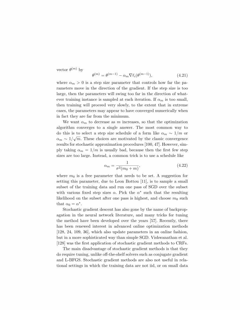
vector θ(m) by

θ(m) = θ(m−1) − αm∇`i(θ(m−1)), (4.21)

where αm > 0 is a step size parameter that controls how far the pa-

rameters move in the direction of the gradient. If the step size is too

large, then the parameters will swing too far in the direction of what-

ever training instance is sampled at each iteration. If αm is too small,

then training will proceed very slowly, to the extent that in extreme

cases, the parameters may appear to have converged numerically when

in fact they are far from the minimum.

We want αm to decrease as m increases, so that the optimization

algorithm converges to a single answer. The most common way to

do this is to select a step size schedule of a form like αm ∼ 1/m or

αm ∼ 1/√m. These choices are motivated by the classic convergence

results for stochastic approximation procedures [100, 47]. However, sim-

ply taking αm = 1/m is usually bad, because then the first few step

sizes are too large. Instead, a common trick is to use a schedule like

αm =1

σ2(m0 +m), (4.22)

where m0 is a free parameter that needs to be set. A suggestion for

setting this parameter, due to Leon Bottou [11], is to sample a small

subset of the training data and run one pass of SGD over the subset

with various fixed step sizes α. Pick the α∗ such that the resulting

likelihood on the subset after one pass is highest, and choose m0 such

that α0 = α∗.

Stochastic gradient descent has also gone by the name of backprop-

agation in the neural network literature, and many tricks for tuning

the method have been developed over the years [57]. Recently, there

has been renewed interest in advanced online optimization methods

[128, 24, 109, 36], which also update parameters in an online fashion,

but in a more sophisticated way than simple SGD. Vishwanathan et al.

[128] was the first application of stochastic gradient methods to CRFs.

The main disadvantage of stochastic gradient methods is that they

do require tuning, unlike off-the-shelf solvers such as conjugate gradient

and L-BFGS. Stochastic gradient methods are also not useful in rela-

tional settings in which the training data are not iid, or on small data

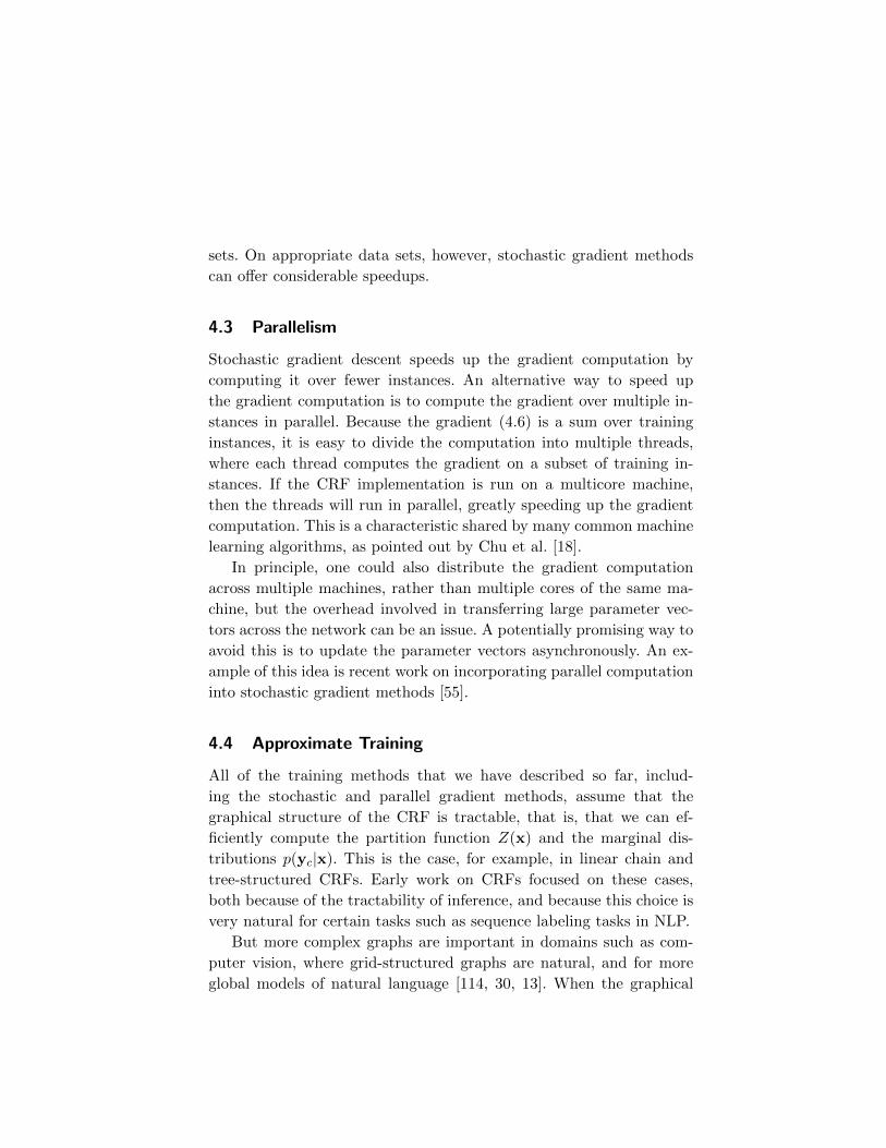
sets. On appropriate data sets, however, stochastic gradient methods

can offer considerable speedups.

4.3 Parallelism

Stochastic gradient descent speeds up the gradient computation by

computing it over fewer instances. An alternative way to speed up

the gradient computation is to compute the gradient over multiple in-

stances in parallel. Because the gradient (4.6) is a sum over training

instances, it is easy to divide the computation into multiple threads,

where each thread computes the gradient on a subset of training in-

stances. If the CRF implementation is run on a multicore machine,

then the threads will run in parallel, greatly speeding up the gradient

computation. This is a characteristic shared by many common machine

learning algorithms, as pointed out by Chu et al. [18].

In principle, one could also distribute the gradient computation

across multiple machines, rather than multiple cores of the same ma-

chine, but the overhead involved in transferring large parameter vec-

tors across the network can be an issue. A potentially promising way to

avoid this is to update the parameter vectors asynchronously. An ex-

ample of this idea is recent work on incorporating parallel computation

into stochastic gradient methods [55].

4.4 Approximate Training

All of the training methods that we have described so far, includ-

ing the stochastic and parallel gradient methods, assume that the

graphical structure of the CRF is tractable, that is, that we can ef-

ficiently compute the partition function Z(x) and the marginal dis-

tributions p(yc|x). This is the case, for example, in linear chain and

tree-structured CRFs. Early work on CRFs focused on these cases,

both because of the tractability of inference, and because this choice is

very natural for certain tasks such as sequence labeling tasks in NLP.

But more complex graphs are important in domains such as com-

puter vision, where grid-structured graphs are natural, and for more

global models of natural language [114, 30, 13]. When the graphical

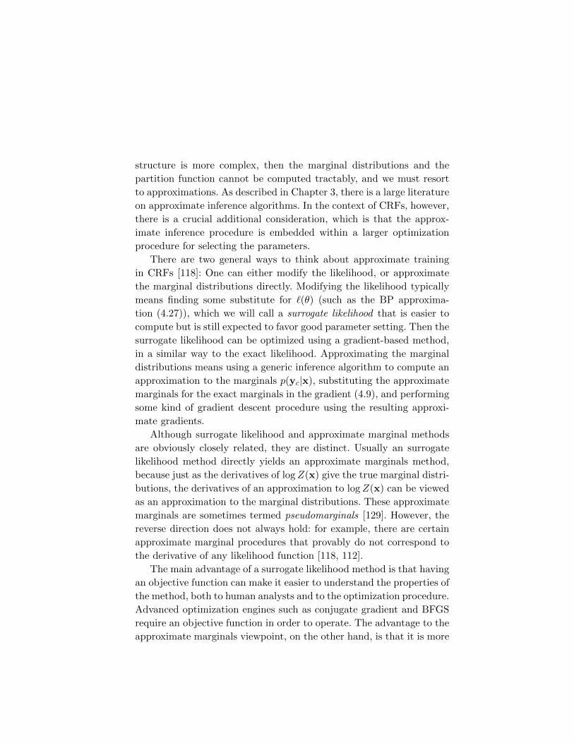
structure is more complex, then the marginal distributions and the

partition function cannot be computed tractably, and we must resort

to approximations. As described in Chapter 3, there is a large literature

on approximate inference algorithms. In the context of CRFs, however,

there is a crucial additional consideration, which is that the approx-

imate inference procedure is embedded within a larger optimization

procedure for selecting the parameters.

There are two general ways to think about approximate training

in CRFs [118]: One can either modify the likelihood, or approximate

the marginal distributions directly. Modifying the likelihood typically

means finding some substitute for `(θ) (such as the BP approxima-

tion (4.27)), which we will call a surrogate likelihood that is easier to

compute but is still expected to favor good parameter setting. Then the

surrogate likelihood can be optimized using a gradient-based method,

in a similar way to the exact likelihood. Approximating the marginal

distributions means using a generic inference algorithm to compute an

approximation to the marginals p(yc|x), substituting the approximate

marginals for the exact marginals in the gradient (4.9), and performing

some kind of gradient descent procedure using the resulting approxi-

mate gradients.

Although surrogate likelihood and approximate marginal methods

are obviously closely related, they are distinct. Usually an surrogate

likelihood method directly yields an approximate marginals method,

because just as the derivatives of logZ(x) give the true marginal distri-

butions, the derivatives of an approximation to logZ(x) can be viewed

as an approximation to the marginal distributions. These approximate

marginals are sometimes termed pseudomarginals [129]. However, the

reverse direction does not always hold: for example, there are certain

approximate marginal procedures that provably do not correspond to

the derivative of any likelihood function [118, 112].

The main advantage of a surrogate likelihood method is that having

an objective function can make it easier to understand the properties of

the method, both to human analysts and to the optimization procedure.

Advanced optimization engines such as conjugate gradient and BFGS

require an objective function in order to operate. The advantage to the

approximate marginals viewpoint, on the other hand, is that it is more

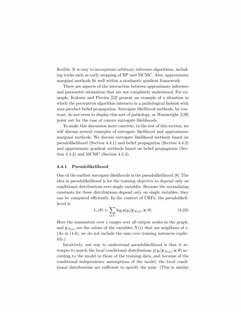
flexible. It is easy to incorporate arbitrary inference algorithms, includ-

ing tricks such as early stopping of BP and MCMC. Also, approximate

marginal methods fit well within a stochastic gradient framework.

There are aspects of the interaction between approximate inference

and parameter estimation that are not completely understood. For ex-

ample, Kulesza and Pereira [52] present an example of a situation in

which the perceptron algorithm interacts in a pathological fashion with

max-product belief propagation. Surrogate likelihood methods, by con-

trast, do not seem to display this sort of pathology, as Wainwright [129]

point out for the case of convex surrogate likelihoods.

To make this discussion more concrete, in the rest of this section, we

will discuss several examples of surrogate likelihood and approximate

marginal methods. We discuss surrogate likelihood methods based on

pseudolikelihood (Section 4.4.1) and belief propagation (Section 4.4.2)

and approximate gradient methods based on belief propagation (Sec-

tion 4.4.2) and MCMC (Section 4.4.3).

4.4.1 Pseudolikelihood

One of the earliest surrogate likelihoods is the pseudolikelihood [8]. The

idea in pseudolikelihood is for the training objective to depend only on

conditional distributions over single variables. Because the normalizing

constants for these distributions depend only on single variables, they

can be computed efficiently. In the context of CRFs, the pseudolikeli-

hood is

`pl(θ) =∑s∈V

log p(ys|yN(s),x; θ) (4.23)

Here the summation over s ranges over all output nodes in the graph,

and yN(s) are the values of the variables N(s) that are neighbors of s.

(As in (4.8), we do not include the sum over training instances explic-

itly.)

Intuitively, one way to understand pseudolikelihood is that it at-

tempts to match the local conditional distributions p(ys|yN(s),x; θ) ac-

cording to the model to those of the training data, and because of the

conditional independence assumptions of the model, the local condi-

tional distributions are sufficient to specify the joint. (This is similar

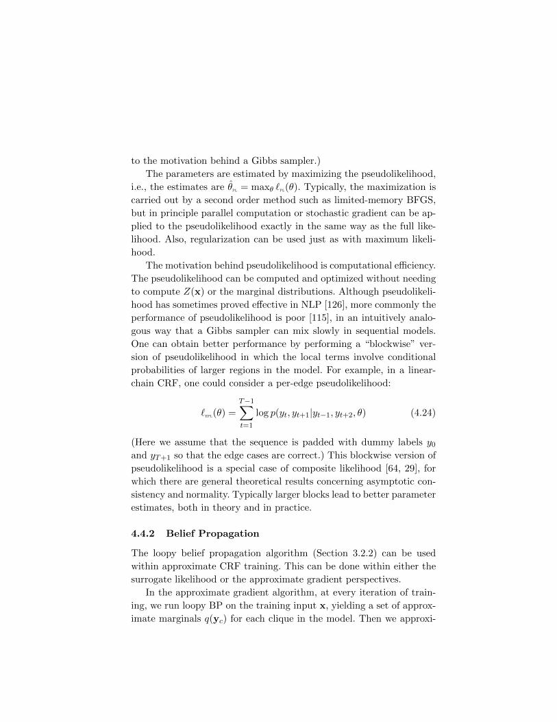
to the motivation behind a Gibbs sampler.)

The parameters are estimated by maximizing the pseudolikelihood,

i.e., the estimates are θpl = maxθ `pl(θ). Typically, the maximization is

carried out by a second order method such as limited-memory BFGS,

but in principle parallel computation or stochastic gradient can be ap-

plied to the pseudolikelihood exactly in the same way as the full like-

lihood. Also, regularization can be used just as with maximum likeli-

hood.

The motivation behind pseudolikelihood is computational efficiency.

The pseudolikelihood can be computed and optimized without needing

to compute Z(x) or the marginal distributions. Although pseudolikeli-

hood has sometimes proved effective in NLP [126], more commonly the

performance of pseudolikelihood is poor [115], in an intuitively analo-

gous way that a Gibbs sampler can mix slowly in sequential models.

One can obtain better performance by performing a “blockwise” ver-

sion of pseudolikelihood in which the local terms involve conditional

probabilities of larger regions in the model. For example, in a linear-

chain CRF, one could consider a per-edge pseudolikelihood:

`epl(θ) =

T−1∑t=1

log p(yt, yt+1|yt−1, yt+2, θ) (4.24)

(Here we assume that the sequence is padded with dummy labels y0

and yT+1 so that the edge cases are correct.) This blockwise version of

pseudolikelihood is a special case of composite likelihood [64, 29], for

which there are general theoretical results concerning asymptotic con-

sistency and normality. Typically larger blocks lead to better parameter

estimates, both in theory and in practice.

4.4.2 Belief Propagation

The loopy belief propagation algorithm (Section 3.2.2) can be used

within approximate CRF training. This can be done within either the

surrogate likelihood or the approximate gradient perspectives.

In the approximate gradient algorithm, at every iteration of train-

ing, we run loopy BP on the training input x, yielding a set of approx-

imate marginals q(yc) for each clique in the model. Then we approxi-

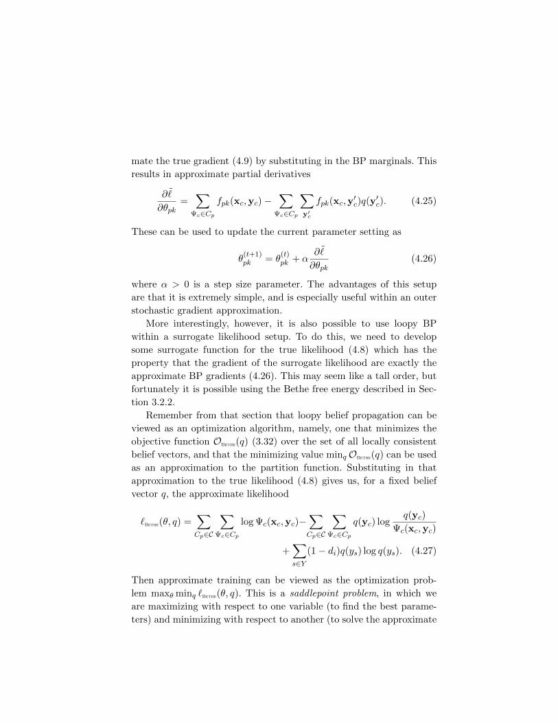
mate the true gradient (4.9) by substituting in the BP marginals. This

results in approximate partial derivatives

∂ ˜

∂θpk=∑

Ψc∈Cp

fpk(xc,yc)−∑

Ψc∈Cp

∑y′c

fpk(xc,y′c)q(y

′c). (4.25)

These can be used to update the current parameter setting as

θ(t+1)pk = θ

(t)pk + α

∂ ˜

∂θpk(4.26)

where α > 0 is a step size parameter. The advantages of this setup

are that it is extremely simple, and is especially useful within an outer

stochastic gradient approximation.

More interestingly, however, it is also possible to use loopy BP

within a surrogate likelihood setup. To do this, we need to develop

some surrogate function for the true likelihood (4.8) which has the

property that the gradient of the surrogate likelihood are exactly the

approximate BP gradients (4.26). This may seem like a tall order, but

fortunately it is possible using the Bethe free energy described in Sec-

tion 3.2.2.

Remember from that section that loopy belief propagation can be

viewed as an optimization algorithm, namely, one that minimizes the

objective function OBethe(q) (3.32) over the set of all locally consistent

belief vectors, and that the minimizing value minqOBethe(q) can be used

as an approximation to the partition function. Substituting in that

approximation to the true likelihood (4.8) gives us, for a fixed belief

vector q, the approximate likelihood

`Bethe(θ, q) =∑Cp∈C

∑Ψc∈Cp

log Ψc(xc,yc)−∑Cp∈C

∑Ψc∈Cp

q(yc) logq(yc)

Ψc(xc,yc)

+∑s∈Y

(1− di)q(ys) log q(ys). (4.27)

Then approximate training can be viewed as the optimization prob-

lem maxθ minq `Bethe(θ, q). This is a saddlepoint problem, in which we

are maximizing with respect to one variable (to find the best parame-

ters) and minimizing with respect to another (to solve the approximate

inference problem). One approach to solve saddlepoint problems is co-

ordinate ascent, that is, to alternately minimize `Bethe with respect to

q for fixed θ and take a gradient step to partially maximize `Bethe with

respect to θ for fixed b. The first step (minimizing with respect to q)

is just running the loopy BP algorithm. The key point is that for the

second step (maximizing with respect to θ), the partial derivatives of

(4.27) with respect to a weight θk is exactly (4.26), as desired.

Alternatively, there is a different surrogate likelihood that can also

be used. This is

ˆ(θ; q) = log

[∏Cp∈C

∏Ψc∈Cp

q(yc)∏s∈Y q(ys)

ds−1

], (4.28)

In other words, instead of the true joint likelihood, we use the product

over each clique’s approximate belief, dividing by the node beliefs to

avoid overcounting. The nice thing about this is that it is a direct

generalisation of the true likelihood for tree-structured models, as can

be seen by comparing (4.28) with (3.27). This surrogate likelihood can

be justified using a dual version of Bethe energy that we have presented

here [78, 81]. When BP has converged, for the resulting belief vector

q, it can be shown that `Bethe(θ, q) = ˆ(θ, q). This equivalence does not

hold in general for arbitrary values of q, e.g., if BP has not converged.

Another surrogate likelihood method that is related to BP is the

piecewise estimator [117], in which the factors of the model are par-

titioned into tractable subgraphs that are trained independently. This

idea can work surprisingly well (better than pseudolikelihood) if the lo-

cal features are sufficiently informative. Sutton and Minka [118] discuss

the close relationship between piecewise training and early stopping of

belief propagation.

4.4.3 Markov Chain Monte Carlo

Markov Chain Monte Carlo (MCMC) inference methods (Section 3.2.1)

can be used within CRF training by setting up a Markov chain whose

stationary distribution is p(y|x; θ), running the chain for a number of

iterations, and using the resulting approximate marginals p(y|x; θ) to

approximate the true marginals in the gradient (4.9).

In practice, however, MCMC methods are not commonly used in the

context of CRFs. There are two main reasons for this. First, MCMC

methods typically require many iterations to reach convergence, and

as we have emphasized, inference needs to be run for many different

parameter settings over the course of training. Second, many MCMC

methods, such as Metropolis-Hastings, require computing a ratio of

normalising constants Zθ1(x)/Zθ2(x) for two different parameters set-

tings θ1 and θ2. This presents a severe difficulty for models in which

computing Zθ(x) is intractable.

One possibility to overcome these difficulties is contrastive diver-

gence (CD) [44], in which the true marginals p(yc|x) in (4.9) are ap-

proximated by running an MCMC method for only a few iterations,

where the initial state of the Markov chain (which is just an assign-

ment to y) is set to be the value of y in the training data. CD has been

mostly applied to latent variable models such as restricted Boltzmann

machines, it can also be applied to CRFs. We are unaware of much

work in this direction.

Another possibility is a more recent method called SampleRank

[135], whose objective is that the learned parameters score pairs of

ys such that their sorted ranking obeys a given supervised ranking

(which is often specified in terms of a fixed scoring function on y that

compares to true target values of y). Approximate gradients may be

calculated from pairs of successive states of the MCMC sampler. Like

CD, SampleRank learns very quickly because it performs useful pa-

rameter updates on many individual MCMC steps. Experiments have

shown the structured classification accuracy from SampleRank to be

substantially higher than CD [135].

The discussion above concerns MCMC methods within an approx-

imate gradient framework. In contrast, it is very difficult to use an

MCMC inference method within an surrogate likelihood framework,

because it is notoriously difficult to obtain a good approximation to

logZ(x) given samples from an MCMC method.

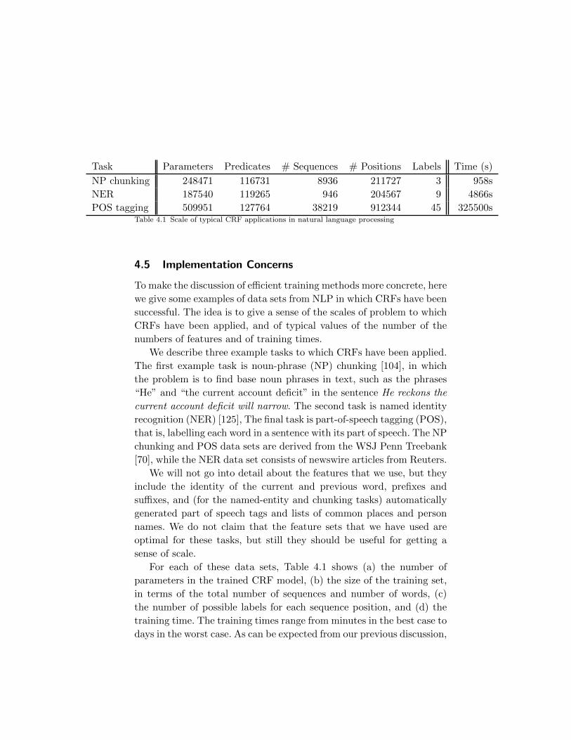
Task Parameters Predicates # Sequences # Positions Labels Time (s)

NP chunking 248471 116731 8936 211727 3 958s

NER 187540 119265 946 204567 9 4866s

POS tagging 509951 127764 38219 912344 45 325500sTable 4.1 Scale of typical CRF applications in natural language processing

4.5 Implementation Concerns

To make the discussion of efficient training methods more concrete, here

we give some examples of data sets from NLP in which CRFs have been

successful. The idea is to give a sense of the scales of problem to which

CRFs have been applied, and of typical values of the number of the

numbers of features and of training times.

We describe three example tasks to which CRFs have been applied.

The first example task is noun-phrase (NP) chunking [104], in which

the problem is to find base noun phrases in text, such as the phrases

“He” and “the current account deficit” in the sentence He reckons the

current account deficit will narrow. The second task is named identity

recognition (NER) [125], The final task is part-of-speech tagging (POS),

that is, labelling each word in a sentence with its part of speech. The NP

chunking and POS data sets are derived from the WSJ Penn Treebank

[70], while the NER data set consists of newswire articles from Reuters.

We will not go into detail about the features that we use, but they

include the identity of the current and previous word, prefixes and

suffixes, and (for the named-entity and chunking tasks) automatically

generated part of speech tags and lists of common places and person

names. We do not claim that the feature sets that we have used are

optimal for these tasks, but still they should be useful for getting a

sense of scale.

For each of these data sets, Table 4.1 shows (a) the number of

parameters in the trained CRF model, (b) the size of the training set,

in terms of the total number of sequences and number of words, (c)

the number of possible labels for each sequence position, and (d) the

training time. The training times range from minutes in the best case to

days in the worst case. As can be expected from our previous discussion,

the factor that seems to most influence training time is the number of

labels.

Obviously the exact training time will depend heavily on details

of the implementation and hardware. For the examples in Table 4.1,

we use the MALLET toolkit on machines with a 2.4 GHz Intel Xeon

CPU, optimizing the likelihood using batch L-BFGS without using mul-

tithreaded or stochastic gradient training.

5

Related Work and Future Directions

In this section, we briefly place CRFs in the context of related lines of

research, especially that of structured prediction, a general research area

which is concerned with extending classification methods to complex

objects. We also describe relationships both to neural networks and

to a simpler sequence model called maximum entropy Markov models

(MEMMs). Finally, we outline a few open areas for future work.

5.1 Related Work

5.1.1 Structured Prediction

Conditional random fields provide one method for extending the ideas

behind classification to the prediction of more complex objects such as

sequences and trees. This general area of research is called structured

prediction. Essentially, logistic regression is to a CRF as classification is

to structured prediction. Examples of the types of structured outputs

that are considered include parse trees of natural language sentences

[123, 31], alignments between sentences in different languages [124], and

route plans in mobile robotics [97]. Detailed information about struc-

tured prediction methods is available in a recent collection of research

63

papers [4].

Structured prediction methods are essentially a combination of clas-

sification and graphical modeling, combining the ability to compactly

model multivariate data with the ability to perform prediction using

large sets of input features. The idea is, for an input x, to define a

discriminant function Fx(y), and predict y∗ = arg maxy Fx(y). This

function factorizes according to a set of local factors, just as in graph-

ical models. But as in classification, each local factor is modeled a lin-

ear function of x, although perhaps in some induced high-dimensional

space. To understand the benefits of this approach, consider a hidden

Markov model (Section 2.2.2) and a set of per-position classifiers, both

with fixed parameters. In principle, the per-position classifiers predict

an output ys given all of x0 . . .xT .1 In the HMM, on the other hand,

to predict ys it is statistically sufficient to know only the local input

xs, the previous forward message p(ys−1,x0 . . .xs−1), and the backward

message p(xs+1 . . .xT |ys). So the forward and backward messages serve

as a summary of the rest of the input, a summary that is generally non-

linear in the observed features.

In principle, the same effect could be achieved using a per-position

classifier if it were possible to define an extremely flexible set of nonlin-

ear features that depend on the entire input sequence. But as we have

seen the size of the input vector is extremely large. For example, in

part-of-speech tagging, each vector xs may have tens of thousands of

components, so a classifier based on all of x would have many param-

eters. But using only xs to predict ys is also bad, because information

from neighboring feature vectors is also useful in making predictions.

Essentially the effect of a structured prediction method is that a confi-

dent prediction about one variable is able to influence nearby, possibly

less confident predictions.

Several types of structured prediction algorithms have been stud-

ied. All such algorithms assume that the discriminant function Fx(y)

over labels can be written as a sum of local functions Fx(y) =∑a fa(ya,x, θ). The task is to estimate the real-valued parameter vec-

1To be fair, in practice the classifier for ys would probably depend only on a sliding windowaround xs, rather than all of x.

tor θ given a training set D = {x(i),y(i)}Ni=1. The methods differ in how

the parameters are selected.

Alternative structured prediction methods are based on maximizing

over assignments rather than marginalizing. Perhaps the most popu-

lar of these methods has been maximum-margin methods that are so

successful for univariate classification. Maximum margin methods have

been generalized to the structured case [2, 122]. Both batch and online

algorithms have been developed to maximize this objective function.

The perceptron update can also be generalized to structured models

[21]. The resulting algorithm is particularly appealing because it is lit-

tle more difficult to implement than the algorithm for selecting y∗. The

online perceptron update can also be made margin-aware, yielding the

MIRA algorithm [23], which may perform better than the perceptron

update.

Another class of methods are search-based methods [27, 28] in which

a heuristic search procedure over outputs is assumed, and learns a clas-

sifier that predicts the next step in the search. This has the advantage

of fitting in nicely to many problems that are complex enough to re-

quire performing search. It is also able to incorporate arbitrary loss

functions over predictions.

A general advantage of all of these maximization-based methods

is that they do not require summation over all configurations for the

partition function or for marginal distributions. There are certain com-

binatorial problems, such as matching and network flow problems, in

which finding an optimal configuration is tractable, but summing over

configurations is not (for an example of applying max-margin methods

in such situations, see Taskar et al. [124]). For more complex problems,

neither summation nor maximization is tractable, so this advantage

is perhaps not as significant. Another advantage of these methods is

that kernels can be naturally incorporated, in an analogous way as in

support vector machines.

Finally, LeCun et al. [59] generalizes many prediction methods, in-

cluding the ones listed above, under the rubric of energy-based methods,

and presents interesting historical information about their use. They

advocate changing the loss function to avoid probabilities altogether.

Perhaps the main advantage of probabilistic methods is that they

can incorporate latent variables in a natural way, by marginalization.

This can be useful, for example, in collective classification methods

[121]. For examples of structured models with latent variables, see

Quattoni et al. [95] and McCallum et al. [75]. A particularly powerful

example of this is provided by Bayesian methods, in which the model

parameters themselves are integrated out (Section 5.2.1).

The differences between the various structured prediction methods

are not well understood. To date, there has been little careful compar-

ison of these, especially CRFs and max-margin approaches, across dif-

ferent structures and domains, although see Keerthi and Sundararajan

[46] for some experiments in this regard.2 We take the view that the

similarities between various structured prediction methods are more

important than the differences. Careful selection of features has more

effect on performance than the choice of structured prediction algo-

rithm.

5.1.2 Neural Networks

There are close relationships between neural networks and conditional

random fields, in that both can be viewed as discriminatively trained

probabilistic models. Neural networks are perhaps best known for their

use in classification, but they can also be used to predict multiple out-

puts, for example, by using a shared latent representation [15], or by

modelling dependencies between outputs directly [58]. Although neural

networks are typically trained using stochastic gradient descent (Sec-

tion 4.2), in principle they can be trained using any of the other meth-

ods used for CRFs. The main difference between them is that neural

networks represent the dependence between output variables using a

shared latent representation, while structured methods learn these de-

pendences as direct functions of the output variables.

Because of this, it is easy to make the mistake of thinking that CRFs

are convex and neural networks are not. This is incorrect. A neural

network without a hidden layer is a linear classifier that can be trained

2An earlier study [86] appears to have been flawed. See Keerthi and Sundararajan [46] fordiscussion.

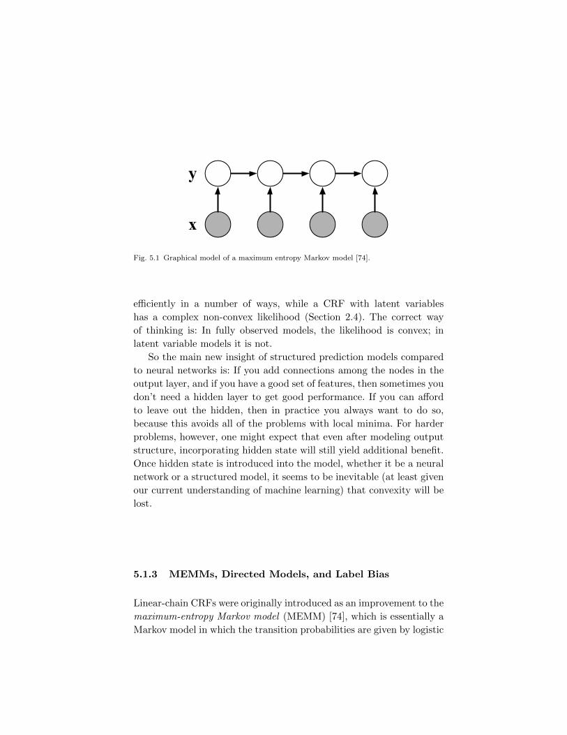
y

x

Fig. 5.1 Graphical model of a maximum entropy Markov model [74].

efficiently in a number of ways, while a CRF with latent variables

has a complex non-convex likelihood (Section 2.4). The correct way

of thinking is: In fully observed models, the likelihood is convex; in

latent variable models it is not.

So the main new insight of structured prediction models compared

to neural networks is: If you add connections among the nodes in the

output layer, and if you have a good set of features, then sometimes you

don’t need a hidden layer to get good performance. If you can afford

to leave out the hidden, then in practice you always want to do so,

because this avoids all of the problems with local minima. For harder

problems, however, one might expect that even after modeling output

structure, incorporating hidden state will still yield additional benefit.

Once hidden state is introduced into the model, whether it be a neural

network or a structured model, it seems to be inevitable (at least given

our current understanding of machine learning) that convexity will be

lost.

5.1.3 MEMMs, Directed Models, and Label Bias

Linear-chain CRFs were originally introduced as an improvement to the

maximum-entropy Markov model (MEMM) [74], which is essentially a

Markov model in which the transition probabilities are given by logistic

regression. Formally, an MEMM is

pMEMM(y|x) =T∏t=1

p(yt|yt−1,x) (5.1)

p(yt|yt−1,x) =1

Zt(yt−1,x)exp

{K∑k=1

θkfk(yt, yt−1,xt)

}(5.2)

Zt(yt−1,x) =∑y′

exp

{K∑k=1

θkfk(y′, yt−1,xt)

}(5.3)

A similar idea can be extended to general directed graphs, in which the

distribution p(y|x) is expressed by a Bayesian network in which each

CPT is a logistic regression models with input x [102].

In the linear-chain case, notice that the MEMM works out to have

the same form as the linear-chain CRF (4.3) with the exception that in a

CRF Z(x) is a sum over sequences, whereas in a MEMM the analogous

term is∏Tt=1 Zt(yt−1,x). This difference has important consequences.

Unlike in a CRFs, maximum likelihood training of MEMMs does not

require performing inference, because Zt is just a simple sum over the

labels at a single position, rather than a sum over labels of an entire

sequence. This is an example of the general phenomenon that training

of directed models is less computationally demanding than undirected

models.

There are theoretical difficulties with the MEMM model, however.

MEMMs can exhibit the problems of label bias [54] and observation

bias [48]. Originally, the label bias problem was described from an al-

gorithmic perspective. Consider the backward recursion (3.9). In the

case of an MEMM, this amounts to

βt(i) =∑j∈S

p(yt+1 = j|yt = i, xt+1)βt+1(j). (5.4)

Unfortunately, this sum is always 1, regardless of the value of the

current label i. To see this, assume for the sake of induction that

βt+1(j) = 1 for all j. Then it is clear that the sum over j in (5.4)

collapses, and βt(i) = 1. What this means is that the future observa-

tions provide no information about the current state, which seems to

lose a major advantage of sequence modelling.

Perhaps a more intuitive way to understand label bias is from the

perspective of graphical models. Consider the graphical model of an

MEMM, shown in Figure 5.1. By looking at the v-structures in the

graph, we can read off the following independence assumptions: at

all time steps t, the label yt is marginally independent of the future

observations xt+1,xt+2, etc. This independence assumption is usually

strongly violated in sequence modeling, which explains why CRFs can

have better performance than MEMMs. Also, this independence rela-

tion explains why βt(i) should always be 1. (In general, this correspon-

dence between graph structure and inference algorithms is one of main

conceptual advantages of graphical modelling.) To summarize this dis-

cussion, label bias is simply a consequence of explaining away.

There is a caveat here: We can always copy information from previ-

ous and future time steps into the feature vector xt, and this is common

in practice. (The only constraint is that if we have too many features,

then overfitting we become an issue.) This has the effect of adding

arcs between (for example) xt+1. This explains why the performance

gap between MEMMs and CRFs is not always as large as might be

expected.

Finally, one might try a different way to combine the advantages of

conditional training and directed models. One can imagine defining a

directed model p(y,x), perhaps a generative model, and then training

it by optimizing the resulting conditional likelihood p(y|x). In fact,

this procedure has long been done in the speech community, where it

is called maximum mutual information training. However, this does

not have strong computational benefits over CRFs. The reason is that

computing the conditional likelihood p(y|x) requires computing the

marginal probability p(x), which plays the same role as Z(x) in the

CRF likelihood. In fact, training is more complex in a directed model,

because the model parameters are constrained to be probabilities—

constraints which can actually make the optimization problem more

difficult.

5.2 Frontier Areas

Finally, we describe a few open research areas that related to CRFs.

In all of the cases below, the research question is a special case of

a larger question for general graphical models, but there are special

additional considerations in conditional models that make the problem

more difficult.

5.2.1 Bayesian CRFs

Because of the large number of parameters in typical applications of

CRFs, the models can be prone to overfitting. The standard way to

control this is using regularization, as described in Section 4.1.1. One

way that we motivated this procedure is as an approximation to a

fully Bayesian procedure. That is, instead of predicting the labels of a

testing instance x as y∗ = maxy p(y|x; θ), where θ is a single parameter

estimate, in a Bayesian method we would use the predictive distribution

y∗ = maxy

∫p(y|x; θ)p(θ)

∏Ni=1 p(y

(i)|x(i), θ)dθ. This integral over θ

needs to be approximated, for example, by MCMC.

In general, it is difficult to formulate efficient Bayesian methods for

undirected models; see [83, 82] for some of the few examples in this

regard. A few papers have specially considered approximate inference

algorithms for Bayesian CRFs [92, 133], but while these methods are

interesting, they do not seem to be useful at the scale of current CRF

applications (e.g., those in Table 4.1). Even for linear chain models,

Bayesian methods are not commonly in use for CRFs, primarily due

to the computational demands. If all we want is the benefits of model

averaging, one may question whether simpler ensemble learning tech-

niques, such as bagging, would give the same benefit. However, the

Bayesian perspective does have other potential benefits, particularly

when more complex, hierarchical priors are considered.

5.2.2 Semi-supervised CRFs

One practical difficulty in applying CRFs is that training requires ob-

taining true labels for potentially many sequences. This can be expen-

sive because it is more time consuming for a human labeller to provide

labels for sequence labelling than for simple classification. For this rea-

son, it would be very useful to have techniques that can obtain good

accuracy given only a small amount of labeled data.

One strategy for achieving this goal is semi-supervised learning,

in which in addition to some fully-labelled data {(x(i),y(i))}Ni=1, the

data set is assumed to contain a large number of unlabelled instances

{x(j)}Mj=1, for which we observe only the inputs. However, unlike in gen-

erative models, it is less obvious how to incorporate unlabelled data

into a conditional criterion, because the unlabelled data is a sample

from the distribution p(x), which in principle need have no relation-

ship to the CRF p(y|x). In order to deal with this, several different

types of regularization terms have been proposed that take the un-

labelled data into account, including entropy regularization [39, 45],

generalized expectation criteria [69], posterior regularization [32, 38],

and measurement-based learning [62].

5.2.3 Structure Learning in CRFs

All of the methods described in this tutorial assume that the structure

of the model has been decided in advance. It is natural to ask if we

can learn the structure of the model as well. As in graphical models

more generally, this is a difficult problem. In fact, Bradley and Guestrin

[12] point out an interesting complication that is specific to conditional

models. Typically, maximum likelihood structure learning can be per-

formed efficiently if the model is restricted to be tree-structured, using

the well-known Chow-Liu algorithm. The analogous algorithm in the

conditional case is more difficult, however, because it requires estimat-

ing marginal distributions of the form p(yu, yv|x1:N ), that is, we need

to estimate the effects of the entire input on every pair of variables. It

is difficult to estimate these distributions efficiently without knowing

the structure of the model to begin with.

Acknowledgments

We thank Francine Chen, Benson Limketkai, Gregory Druck, Kedar

Bellare, and Ray Mooney for useful comments on earlier versions of this

tutorial. A previous version of this tutorial has appeared in Sutton and

McCallum [116], and as part of Charles Sutton’s doctoral dissertation

[113].

References

[1] Srinivas M. Aji and Robert J. McEliece. The generalized dis-

tributive law. IEEE Transactions on Information Theory, 46(2):

325–343, 2000.

[2] Yasemin Altun, Ioannis Tsochantaridis, and Thomas Hofmann.

Hidden Markov support vector machines. In International Con-

ference on Machine Learning (ICML), 2003.

[3] Galen Andrew and Jianfeng Gao. Scalable training of l1-

regularized log-linear models. In International Conference on

Machine Learning (ICML), 2007.

[4] Gokhan H. Bakir, Thomas Hofmann, Bernhard Scholkopf,

Alexander J. Smola, Ben Taskar, and S. V. N. Vishwanathan,

editors. Predicting Structured Data. MIT Press, 2007.

[5] Axel Bernal, Koby Crammer, Artemis Hatzigeorgiou, and Fer-

nando Pereira. Global discriminative learning for higher-accuracy

computational gene prediction. PLoS Computational Biology, 3

(3), 2007.

[6] Dimitri P. Bertsekas. Nonlinear Programming. Athena Scientific,

2nd edition, 1999.

[7] Julian Besag. Spatial interaction and the statistical analysis of

73

lattice systems. Journal of the Royal Statistical Society. Series

B, 36(2):192–236, 1974.

[8] Julian Besag. Statistical analysis of non-lattice data. The Statis-

tician, 24(3):179–195, 1975.

[9] David M. Blei, Andrew Y. Ng, and Michael I. Jordan. Latent

dirichlet allocation. Journal of Machine Learning Research, 3:

993, 2003.

[10] Phil Blunsom and Trevor Cohn. Discriminative word alignment

with conditional random fields. In International Conference on

Computational Linguistics and 44th Annual Meeting of the As-

sociation for Computational Linguistics (COLING-ACL), pages

65–72, 2006.

[11] Leon Bottou. Stochastic gradient descent examples on toy prob-

lems. 2010. URL http://leon.bottou.org/projects/sgd.

[12] Joseph K. Bradley and Carlos Guestrin. Learning tree conditional

random fields. In International Conference on Machine Learning

(ICML 2010), 2010.

[13] Razvan Bunescu and Raymond J. Mooney. Collective information

extraction with relational Markov networks. In Proceedings of

the 42nd Annual Meeting of the Association for Computational

Linguistics, 2004.

[14] Richard H. Byrd, Jorge Nocedal, and Robert B. Schnabel. Rep-

resentations of quasi-Newton matrices and their use in limited

memory methods. Math. Program., 63(2):129–156, 1994. ISSN

0025-5610.

[15] Rich Caruana. Multitask learning. Machine Learning, 28(1):

41–75, 1997. ISSN 0885-6125. doi: http://dx.doi.org/10.1023/A:

1007379606734.

[16] Rich Caruana and Alexandru Niculescu-Mizil. An empirical com-

parison of supervised learning algorithms using different perfor-

mance metrics. Technical Report TR2005-1973, Cornell Uni-

versity, 2005. http://www.niculescu-mizil.org/paper.php?

p=comparison.tr.pdf.

[17] Yejin Choi, Claire Cardie, Ellen Riloff, and Siddharth Patward-

han. Identifying sources of opinions with conditional random

fields and extraction patterns. In Proceedings of the Human Lan-

guage Technology Conference/Conference on Empirical Methods

in Natural Language Processing (HLT-EMNLP), 2005.

[18] C.T. Chu, S.K. Kim, Y.A. Lin, Y.Y. Yu, G. Bradski, A.Y. Ng,

and K. Olukotun. Map-reduce for machine learning on multicore.

In Advances in Neural Information Processing Systems 19, pages

281–288. MIT Press, 2007.

[19] Stephen Clark and James R. Curran. Parsing the WSJ using

CCG and log-linear models. In Proceedings of the 42nd Meeting

of the Association for Computational Linguistics (ACL), pages

103–110, 2004.

[20] Trevor Cohn. Efficient inference in large conditional random

fields. In European Conference on Machine Learning (ECML),

pages 606–613, Berlin, Germany, September 2006.

[21] Michael Collins. Discriminative training methods for hidden

Markov models: Theory and experiments with perceptron algo-

rithms. In Conference on Empirical Methods in Natural Language

Processing (EMNLP), 2002.

[22] Philip J. Cowans and Martin Szummer. A graphical model for si-

multaneous partitioning and labeling. In Conference on Artificial

Intelligence and Statistics (AISTATS), 2005.

[23] Koby Crammer and Yoram Singer. Ultraconservative online al-

gorithms for multiclass problems. Journal of Machine Learning

Research, 3:951–991, Jan 2003.

[24] Koby Crammer, Ofer Dekel, Joseph Keshet, Shai Shalev-Shwartz,

and Yoram Singer. Online passive-aggressive algorithms. Journal

of Machine Learning Research, 2006.

[25] Aron Culotta and Andrew McCallum. Confidence estimation for

information extraction. In Human Language Technology Confer-

ence (HLT), 2004.

[26] Aron Culotta, Ron Bekkerman, and Andrew McCallum. Ex-

tracting social networks and contact information from email and

the web. In First Conference on Email and Anti-Spam (CEAS),

Mountain View, CA, 2004.

[27] Hal Daume III and Daniel Marcu. Learning as search op-

timization: Approximate large margin methods for structured

prediction. In International Conference on Machine Learning

(ICML), Bonn, Germany, 2005. URL http://pub.hal3.name/

#daume05laso.

[28] Hal Daume III, John Langford, and Daniel Marcu. Search-based

structured prediction. Machine Learning Journal, 2009.

[29] Joshua Dillon and Guy Lebanon. Statistical and computational

tradeoffs in stochastic composite likelihood. arXiv:1003.0691v1,

2010.

[30] Jenny Finkel, Trond Grenager, and Christopher D. Manning.

Incorporating non-local information into information extraction

systems by Gibbs sampling. In Proceedings of the 43rd Annual

Meeting of the Association for Computational Linguistics (ACL),

2005.

[31] Jenny Rose Finkel, Alex Kleeman, and Christopher D. Manning.

Efficient, feature-based, conditional random field parsing. In An-

nual Meeting of the Association for Computational Linguistics

(ACL/HLT), pages 959–967, 2008.

[32] Kuzman Ganchev, Joao Graca, Jennifer Gillenwater, and Ben

Taskar. Posterior regularization for structured latent variable

models. Technical Report MS-CIS-09-16, University of Pennsyl-

vania Department of Computer and Information Science, 2009.

[33] Alan E. Gelfand and Adrian F. M. Smith. Sampling-based ap-

proaches to calculating marginal densities. Journal of the Amer-

ican Statistical Association, 85:398–409, 1990.

[34] Stuart Geman and Donald Geman. Stochastic relaxation, Gibbs

distributions, and the Bayesian restoration of images. IEEE

Transactions on Pattern Analysis and Machine Intelligence, 6:

721–741, 1984.

[35] Nadia Ghamrawi and Andrew McCallum. Collective multi-label

classification. In Conference on Information and Knowledge

Management (CIKM), 2005.

[36] Amir Globerson, Terry Koo, Xavier Carreras, and Michael

Collins. Exponentiated gradient algorithms for log-linear struc-

tured prediction. In International Conference on Machine Learn-

ing (ICML), 2007.

[37] Joshua Goodman. Exponential priors for maximum entropy mod-

els. In Proceedings of the Human Language Technology Confer-

ence/North American Chapter of the Association for Computa-

tional Linguistics (HLT/NAACL), 2004.

[38] Joao Graca, Kuzman Ganchev, Ben Taskar, and Fernando

Pereira. Posterior vs parameter sparsity in latent variable models.

In Y. Bengio, D. Schuurmans, J. Lafferty, C. K. I. Williams, and

A. Culotta, editors, Advances in Neural Information Processing

Systems 22, pages 664–672. 2009.

[39] Yves Grandvalet and Yoshua Bengio. Semi-supervised learning

by entropy minimization. In Advances in Neural Information

Processing Systems, 2004.

[40] Michelle L. Gregory and Yasemin Altun. Using conditional ran-

dom fields to predict pitch accents in conversational speech. In

Annual Meeting of the Association for Computational Linguis-

tics (ACL), pages 677–683, 2004. doi: http://dx.doi.org/10.3115/

1218955.1219041.

[41] Asela Gunawardana, Milind Mahajan Alex Acero, and John C.

Platt. Hidden conditional random fields for phone classification.

In International Conference on Speech Communication and Tech-

nology, 2005.

[42] John M. Hammersley and Peter Clifford. Markov fields on finite

graphs and lattices. 1971.

[43] Xuming He, Richard S. Zemel, and Miguel A. Carreira-Perpinian.

Multiscale conditional random fields for image labelling. In IEEE

Computer Society Conference on Computer Vision and Pattern

Recognition, 2004.

[44] Geoffrey E. Hinton. Training products of experts by minimizing

contrastive divergence. Neural Computation, 14:1771–1800, 2002.

[45] F. Jiao, S. Wang, C. Lee, R. Greiner, and D Schuurmans. Semi-

supervised conditional random fields for improved sequence seg-

mentation and labeling. In Joint Conference of the International

Committee on Computational Linguistics and the Association for

Computational Linguistics (COLING/ACL), 2006.

[46] S. Sathiya Keerthi and S. Sundararajan. CRF versus

SVM-struct for sequence labeling. Technical report, Ya-

hoo! Research, 2007. URL http://www.keerthis.com/crf_

comparison_keerthi_07.pdf.

[47] J. Kiefer and J. Wolfowitz. Stochastic estimation of the maximum

of a regression function. Annals of Mathematical Statistics, 23:

462–466, 1952.

[48] Dan Klein and Christopher D. Manning. Conditional structure

versus conditional estimation in NLP models. In Conference on

Empirical Methods in Natural Language Processing (EMNLP),

2002.

[49] Daphne Koller and Nir Friedman. Probabilistic Graphical Models:

Principles and Techniques. MIT Press, 2009.

[50] Frank R. Kschischang, Brendan J. Frey, and Hans-Andrea

Loeliger. Factor graphs and the sum-product algorithm. IEEE

Transactions on Information Theory, 47(2):498–519, 2001.

[51] Taku Kudo, Kaoru Yamamoto, and Yuji Matsumoto. Applying

conditional random fields to Japanese morphological analysis. In

Proceedings of the Conference on Empirical Methods in Natural

Language Processing (EMNLP), 2004.

[52] Alex Kulesza and Fernando Pereira. Structured learning with

approximate inference. In Advances in Neural Information Pro-

cessing Systems, 2008.

[53] Sanjiv Kumar and Martial Hebert. Discriminative fields for mod-

eling spatial dependencies in natural images. In Sebastian Thrun,

Lawrence Saul, and Bernhard Scholkopf, editors, Advances in

Neural Information Processing Systems (NIPS)16. MIT Press,

Cambridge, MA, 2003.

[54] John Lafferty, Andrew McCallum, and Fernando Pereira. Con-

ditional random fields: Probabilistic models for segmenting and

labeling sequence data. International Conference on Machine

Learning (ICML), 2001.

[55] John Langford, Alex Smola, and Martin Zinkevich. Slow learn-

ers are fast. In Y. Bengio, D. Schuurmans, J. Lafferty, C. K. I.

Williams, and A. Culotta, editors, Advances in Neural Informa-

tion Processing Systems 22, pages 2331–2339, 2009.

[56] T. Lavergne, O. Cappe, and F. Yvon. Practical very large scale

crfs. In Proc. 48th Annual Meeting Association for Computa-

tional Linguistics (ACL), pages 504–513, 2010.

[57] Yann Le Cun, Leon Bottou, Genevieve B. Orr, and Klaus-

Robert Muller. Efficient backprop. In Neural Networks, Tricks

of the Trade, Lecture Notes in Computer Science LNCS 1524.

Springer Verlag, 1998. URL http://leon.bottou.org/papers/

lecun-98x.

[58] Yann LeCun, Leon Bottou, Yoshua Bengio, and Patrick Haffner.

Gradient-based learning applied to document recognition. Pro-

ceedings of the IEEE, 86(11):2278–2324, November 1998.

[59] Yann LeCun, Sumit Chopra, Raia Hadsell, Ranzato

Marc’Aurelio, and Fu-Jie Huang. A tutorial on energy-

based learning. In G. Bakir, T. Hofman, B. Scholkopf, A. Smola,

and B. Taskar, editors, Predicting Structured Data. MIT Press,

2007.

[60] Stan Z. Li. Markov Random Field Modeling in Image Analysis.

Springer-Verlag, 2001.

[61] P. Liang and M.I. Jordan. An asymptotic analysis of generative,

discriminative, and pseudolikelihood estimators. In International

Conference on Machine Learning (ICML), pages 584–591. ACM,

2008.

[62] P. Liang, M. I. Jordan, and D. Klein. Learning from measure-

ments in exponential families. In International Conference on

Machine Learning (ICML), 2009.

[63] Chih-Jen Lin, Ruby Chiu-Hsing Weng, and Sathiya Keerthi.

Trust region newton methods for large-scale logistic regression.

In Interational Conference on Machine Learning (ICML), 2007.

[64] Bruce G. Lindsay. Composite likelihood methods. Contemporary

Mathematics, pages 221–239, 1988.

[65] Yan Liu, Jaime Carbonell, Peter Weigele, and Vanathi Gopalakr-

ishnan. Protein fold recognition using segmentation conditional

random fields (SCRFs). Journal of Computational Biology, 13

(2):394–406, 2006.

[66] David J. Lunn, Andrew Thomas, Nicky Best, and David Spiegel-

halter. WinBUGS—a Bayesian modelling framework: Concepts,

structure, and extensibility. Statistics and Computing, 10(4):325–

337, 2000.

[67] David J. C. MacKay. Information Theory, Inference, and Learn-

ing Algorithms. Cambridge University Press, 2003.

[68] Robert Malouf. A comparison of algorithms for maximum

entropy parameter estimation. In Dan Roth and Antal

van den Bosch, editors, Conference on Natural Language Learn-

ing (CoNLL), pages 49–55, 2002.

[69] Gideon Mann and Andrew McCallum. Generalized expectation

criteria for semi-supervised learning of conditional random fields.

In Proceedings of Association of Computational Linguistics, 2008.

[70] Mitchell P. Marcus, Beatrice Santorini, and Mary Ann

Marcinkiewicz. Building a large annotated corpus of English:

The Penn Treebank. Computational Linguistics, 19(2):313–330,

1993.

[71] Andrew McCallum. Efficiently inducing features of conditional

random fields. In Conference on Uncertainty in AI (UAI), 2003.

[72] Andrew McCallum and Wei Li. Early results for named entity

recognition with conditional random fields, feature induction and

web-enhanced lexicons. In Seventh Conference on Natural Lan-

guage Learning (CoNLL), 2003.

[73] Andrew McCallum and Ben Wellner. Conditional models of

identity uncertainty with application to noun coreference. In

Lawrence K. Saul, Yair Weiss, and Leon Bottou, editors, Ad-

vances in Neural Information Processing Systems 17, pages 905–

912. MIT Press, Cambridge, MA, 2005.

[74] Andrew McCallum, Dayne Freitag, and Fernando Pereira. Maxi-

mum entropy Markov models for information extraction and seg-

mentation. In International Conference on Machine Learning

(ICML), pages 591–598. Morgan Kaufmann, San Francisco, CA,

2000.

[75] Andrew McCallum, Kedar Bellare, and Fernando Pereira. A

conditional random field for discriminatively-trained finite-state

string edit distance. In Conference on Uncertainty in AI (UAI),

2005.

[76] Andrew McCallum, Karl Schultz, and Sameer Singh. Facto-

rie: Probabilistic programming via imperatively defined factor

graphs. In Advances on Neural Information Processing Systems

(NIPS), 2009.

[77] Robert J. McEliece, David J. C. MacKay, and Jung-Fu Cheng.

Turbo decoding as an instance of Pearl’s “belief propagation”

algorithm. IEEE Journal on Selected Areas in Communications,

16(2):140–152, 1998.

[78] Thomas P. Minka. The EP energy function and minimization

schemes. Technical report, 2001. http://research.microsoft.

com/~minka/papers/ep/minka-ep-energy.pdf.

[79] Thomas P. Minka. A comparsion of numerical optimizers for

logistic regression. Technical report, 2003. http://research.

microsoft.com/~minka/papers/logreg/.

[80] Tom Minka. Discriminative models, not discriminative train-

ing. Technical Report MSR-TR-2005-144, Microsoft Research,

October 2005. ftp://ftp.research.microsoft.com/pub/tr/

TR-2005-144.pdf.

[81] Tom Minka. Divergence measures and message passing. Technical

Report MSR-TR-2005-173, Microsoft Research, 2005.

[82] Iain Murray. Advances in Markov chain Monte Carlo methods.

PhD thesis, Gatsby computational neuroscience unit, University

College London, 2007.

[83] Iain Murray, Zoubin Ghahramani, and David J. C. MacKay.

MCMC for doubly-intractable distributions. In Uncertainty in

Artificial Intelligence (UAI), pages 359–366. AUAI Press, 2006.

[84] Andrew Y. Ng. Feature selection, l1 vs. l2 regularization, and

rotational invariance. In International Conference on Machine

Learning (ICML), 2004.

[85] Andrew Y. Ng and Michael I. Jordan. On discriminative vs. gen-

erative classifiers: A comparison of logistic regression and naive

bayes. In Thomas G. Dietterich, Suzanna Becker, and Zoubin

Ghahramani, editors, Advances in Neural Information Processing

Systems 14, pages 841–848, Cambridge, MA, 2002. MIT Press.

[86] N. Nguyen and Y. Guo. Comparisons of sequence labeling algo-

rithms and extensions. In International Conference on Machine

Learning (ICML), 2007.

[87] Jorge Nocedal and Stephen J. Wright. Numerical Optimization.

Springer-Verlag, New York, 1999. ISBN 0-387-98793-2.

[88] Judea Pearl. Probabilistic Reasoning in Intelligent Systems: Net-

works of Plausible Inference. Morgan Kaufmann, 1988.

[89] Fuchun Peng and Andrew McCallum. Accurate information ex-

traction from research papers using conditional random fields.

In Proceedings of Human Language Technology Conference and

North American Chapter of the Association for Computational

Linguistics (HLT-NAACL’04), 2004.

[90] Fuchun Peng, Fangfang Feng, and Andrew McCallum. Chinese

segmentation and new word detection using conditional random

fields. In Proceedings of The 20th International Conference on

Computational Linguistics (COLING), pages 562–568, 2004.

[91] David Pinto, Andrew McCallum, Xing Wei, and W. Bruce Croft.

Table extraction using conditional random fields. In Proceedings

of the ACM SIGIR, 2003.

[92] Yuan Qi, Martin Szummer, and Thomas P. Minka. Bayesian

conditional random fields. In Conference on Artificial Intelligence

and Statistics (AISTATS), 2005.

[93] Yuan Qi, Martin Szummer, and Thomas P. Minka. Diagram

structure recognition by Bayesian conditional random fields.

In International Conference on Computer Vision and Pattern

Recognition, 2005.

[94] A. Quattoni, S. Wang, L.P. Morency, M. Collins, and T. Darrell.

Hidden-state conditional random fields. IEEE PAMI, 2007.

[95] Ariadna Quattoni, Michael Collins, and Trevor Darrell. Condi-

tional random fields for object recognition. In Lawrence K. Saul,

Yair Weiss, and Leon Bottou, editors, Advances in Neural In-

formation Processing Systems 17, pages 1097–1104. MIT Press,

Cambridge, MA, 2005.

[96] Lawrence R. Rabiner. A tutorial on hidden Markov models and

selected applications in speech recognition. Proceedings of the

IEEE, 77(2):257 – 286, 1989.

[97] Nathan Ratliff, J. Andrew Bagnell, and Martin Zinkevich. Max-

imum margin planning. In International Conference on Machine

Learning, July 2006.

[98] Matthew Richardson and Pedro Domingos. Markov logic net-

works. Machine Learning, 62(1–2):107–136, 2006.

[99] Stefan Riezler, Tracy King, Ronald Kaplan, Richard Crouch,

John T. Maxwell III, and Mark Johnson. Parsing the Wall Street

Journal using a lexical-functional grammar and discriminative es-

timation techniques. In Proceedings of the 40th Annual Meeting

of the Association for Computational Linguistics, 2002.

[100] H. Robbins and S. Monro. A stochastic approximation method.

Annals of Mathematical Statistics, 22:400–407, 1951.

[101] Christian Robert and George Casella. Monte Carlo Statistical

Methods. Springer, 2004.

[102] David Rosenberg, Dan Klein, and Ben Taskar. Mixture-of-parents

maximum entropy Markov models. In Conference on Uncertainty

in Artificial Intelligence (UAI), 2007.

[103] Dan Roth and Wen-tau Yih. Integer linear programming infer-

ence for conditional random fields. In International Conference

on Machine Learning (ICML), pages 737–744, 2005.

[104] Erik F. Tjong Kim Sang and Sabine Buchholz. Introduction

to the CoNLL-2000 shared task: Chunking. In Proceedings of

CoNLL-2000 and LLL-2000, 2000. See http://lcg-www.uia.

ac.be/~erikt/research/np-chunking.html.

[105] Sunita Sarawagi and William W. Cohen. Semi-Markov condi-

tional random fields for information extraction. In Lawrence K.

Saul, Yair Weiss, and Leon Bottou, editors, Advances in Neural

Information Processing Systems 17, pages 1185–1192. MIT Press,

Cambridge, MA, 2005.

[106] Kengo Sato and Yasubumi Sakakibara. RNA sec-

ondary structural alignment with conditional ran-

dom fields. Bioinformatics, 21:ii237–242, 2005. URL

http://bioinformatics.oxfordjournals.org/cgi/content/

abstract/21/suppl_2/ii237.

[107] Burr Settles. Abner: an open source tool for automatically tag-

ging genes, proteins, and other entity names in text. Bioinfor-

matics, 21(14):3191–3192, 2005.

[108] Fei Sha and Fernando Pereira. Shallow parsing with conditional

random fields. In Conference on Human Language Technology

and North American Association for Computational Linguistics

(HLT-NAACL), pages 213–220, 2003.

[109] Shai Shalev-Shwartz, Yoram Singer, and Nathan Srebro. Pegasos:

Primal estimated sub-gradient solver for SVM. In International

Conference on Machine Learning (ICML), 2007.

[110] P. Singla and P. Domingos. Discriminative training of Markov

logic networks. In Proceedings of the Twentieth National Con-

ference on Artificial Intelligence, pages 868–873, Pittsburgh, PA,

2005. AAAI Press.

[111] David H. Stern, Thore Graepel, and David J. C. MacKay. Mod-

elling uncertainty in the game of go. In Lawrence K. Saul, Yair

Weiss, and Leon Bottou, editors, Advances in Neural Information

Processing Systems 17, pages 1353–1360. MIT Press, Cambridge,

MA, 2005.

[112] Ilya Sutskever and Tijmen Tieleman. On the convergence prop-

erties of contrastive divergence. In Conference on Artificial In-

telligence and Statistics (AISTATS), 2010.

[113] Charles Sutton. Efficient Training Methods for Conditional Ran-

dom Fields. PhD thesis, University of Massachusetts, 2008.

[114] Charles Sutton and Andrew McCallum. Collective segmenta-

tion and labeling of distant entities in information extraction. In

ICML Workshop on Statistical Relational Learning and Its Con-

nections to Other Fields, 2004.

[115] Charles Sutton and Andrew McCallum. Piecewise training of

undirected models. In Conference on Uncertainty in Artificial

Intelligence (UAI), 2005.

[116] Charles Sutton and Andrew McCallum. An introduction to con-

ditional random fields for relational learning. In Lise Getoor and

Ben Taskar, editors, Introduction to Statistical Relational Learn-

ing. MIT Press, 2007.

[117] Charles Sutton and Andrew McCallum. Piecewise training for

structured prediction. Machine Learning, 77(2–3):165–194, 2009.

[118] Charles Sutton and Tom Minka. Local training and belief propa-

gation. Technical Report TR-2006-121, Microsoft Research, 2006.

[119] Charles Sutton, Khashayar Rohanimanesh, and Andrew McCal-

lum. Dynamic conditional random fields: Factorized probabilistic

models for labeling and segmenting sequence data. In Interna-

tional Conference on Machine Learning (ICML), 2004.

[120] Charles Sutton, Andrew McCallum, and Khashayar Rohani-

manesh. Dynamic conditional random fields: Factorized proba-

bilistic models for labeling and segmenting sequence data. Jour-

nal of Machine Learning Research, 8:693–723, March 2007. URL

publications/jmlr-sutton07a.pdf.

[121] Ben Taskar, Pieter Abbeel, and Daphne Koller. Discriminative

probabilistic models for relational data. In Conference on Uncer-

tainty in Artificial Intelligence (UAI), 2002.

[122] Ben Taskar, Carlos Guestrin, and Daphne Koller. Max-margin

Markov networks. In Sebastian Thrun, Lawrence Saul, and Bern-

hard Scholkopf, editors, Advances in Neural Information Process-

ing Systems 16. MIT Press, Cambridge, MA, 2004.

[123] Ben Taskar, Dan Klein, Michael Collins, Daphne Koller, and

Christopher Manning. Max-margin parsing. In Empirical Meth-

ods in Natural Language Processing (EMNLP04), 2004.

[124] Ben Taskar, Simon Lacoste-Julien, and Dan Klein. A discrimi-

native matching approach to word alignment. In Conference on

Human Language Technology and Empirical Methods in Natural

Language Processing (HLT-EMNLP), pages 73–80, 2005.

[125] Erik F. Tjong Kim Sang and Fien De Meulder. Introduction to

the conll-2003 shared task: Language-independent named entity

recognition. In Walter Daelemans and Miles Osborne, editors,

Proceedings of CoNLL-2003, pages 142–147. Edmonton, Canada,

2003.

[126] Kristina Toutanova, Dan Klein, Christopher D. Manning, and

Yoram Singer. Feature-rich part-of-speech tagging with a cyclic

dependency network. In HLT-NAACL, 2003.

[127] Paul Viola and Mukund Narasimhan. Learning to extract infor-

mation from semi-structured text using a discriminative context

free grammar. In Proceedings of the ACM SIGIR, 2005.

[128] S.V.N. Vishwanathan, Nicol N. Schraudolph, Mark W. Schmidt,

and Kevin Murphy. Accelerated training of conditional random

fields with stochastic meta-descent. In International Conference

on Machine Learning (ICML), pages 969–976, 2006.

[129] Martin J. Wainwright. Estimating the wrong Markov random

field: Benefits in the computation-limited setting. In Y. Weiss,

B. Scholkopf, and J. Platt, editors, Advances in Neural Informa-

tion Processing Systems 18. MIT Press, Cambridge, MA, 2006.

[130] Martin J. Wainwright and Michael I. Jordan. Graphical models,

exponential families, and variational inference. Technical Report

Technical Report 649, UC Berkeley, Dept. of Statistics, Septem-

ber 2003.

[131] M.J. Wainwright and M.I. Jordan. Graphical models, exponential

families, and variational inference. Foundations and Trends in

Machine Learning, 1(1-2):1–305, 2008.

[132] Hanna Wallach. Efficient training of conditional random fields.

M.Sc. thesis, University of Edinburgh, 2002.

[133] Max Welling and Sridevi Parise. Bayesian random fields: The

Bethe-Laplace approximation. In Uncertainty in Artificial Intel-

ligence (UAI), 2006.

[134] Michael Wick, Khashayar Rohanimanesh, Andrew McCallum,

and AnHai Doan. A discriminative approach to ontology align-

ment. In International Workshop on New Trends in Information

Integration (NTII), 2008.

[135] Michael Wick, Khashayar Rohanimanesh, Aron Culotta, and An-

drew McCallum. Samplerank: Learning preferences from atomic

gradients. In Neural Information Processing Systems (NIPS)

Workshop on Advances in Ranking, 2009.

[136] Jonathan S. Yedidia, William T. Freeman, and Yair Weiss. Con-

structing free energy approximations and generalized belief prop-

agation algorithms. Technical Report TR2004-040, Mitsubishi

Electric Research Laboratories, 2004.

[137] Jonathan S. Yedidia, William T. Freeman, and Yair Weiss. Con-

structing free-energy approximations and generalized belief prop-

agation algorithms. IEEE Transactions on Information Theory,

51(7):2282–2312, July 2005.

[138] Jin Yu, S.V.N. Vishwanathan, Simon Guunter, and Nicol N.

Schraudolph. A quasi-Newton approach to nonsmooth convex

optimization problems in machine learning. Journal of Machine

Learning Research, 11:1145–1200, Mar 2010.