An optimal online algorithm for single machine scheduling with bounded delivery times

European Journal of Operational Research 201 (2010) 693–700

Contents lists available at ScienceDirect

European Journal of Operational Research

journal homepage: www.elsevier .com/locate /e jor

Discrete Optimization

An optimal online algorithm for single machine schedulingwith bounded delivery times

Ming Liu a,b,*, Chengbin Chu a,b, Yinfeng Xu a, Feifeng Zheng a

a School of Management, Xi’an Jiaotong University, Xi’an, Shaanxi Province 710049, PR Chinab Laboratoire Génie Industriel, Ecole Centrale Paris, Grande Voie des Vignes, 92295 Châtenay-Malabry Cedex, France

a r t i c l e i n f o

Article history:Received 24 October 2008Accepted 20 March 2009Available online 29 March 2009

Keywords:Online schedulingDelivery timeCompetitive analysisSingle machine

0377-2217/$ - see front matter � 2009 Elsevier B.V. Adoi:10.1016/j.ejor.2009.03.028

* Corresponding author. Address: Laboratoire GénParis, Grande Voie des Vignes, 92295 Châtenay-Malab

E-mail addresses: [email protected] (M. Liu), [email protected] (Y. Xu), [email protected].

a b s t r a c t

We study an online scheduling problem on a single machine with delivery times. The problem is online inthe sense that all jobs arrive over time. Each job’s characteristics, such as processing time and deliverytime, become known at its arrival time. Preemption is not allowed and once the processing of a job iscompleted we delivery it to the destination by a vehicle. The objective is to minimize the time by whichall jobs have been delivered. In this paper, we assume that all jobs have bounded delivery times, whichmeans that given a certain positive number b P 1

2, for each job Jj , we have a release time rj P 0 andbqj 6 pj, where pj; qj denote the processing time and the delivery time of job Jj, respectively. We use1jonline; rj; bqj 6 pjjLmax to denote the problem for short, where Lmax denote the time by which all jobshave been delivered. We prove a lower bound of competitive ratios for all online algorithms and propose

an optimal online algorithm with a competitive ratio of 12

ffiffiffiffiffiffiffiffiffiffiffiffiffiffiffiffiffiffiffiffiffiffiffiffiffi5þ b2 þ 2b

qþ 1� b

� �.

� 2009 Elsevier B.V. All rights reserved.

1. Introduction

In recent years, one of the basic assumptions made in determin-istic scheduling was that all the useful information of the probleminstance was known in advance. However, this assumption is usu-ally not practical. This reason promotes the emergence of onlinescheduling. Three online models are commonly considered [2].The first one assumes that there are no release dates and thatthe jobs arrive in a list. An online algorithm has to schedule thefirst job in this list before it sees the next job in the list. The secondmodel assumes that the running time of a job is unknown until thejob finishes. The online algorithm online knows whether a job isstill running or not. The third model assumes that jobs arrive overtime. At each time when the machine is idle, the algorithm decideswhich one of the available jobs is scheduled, if any. If all informa-tion are available at the beginning (before scheduling), we callthese problems offline. In this paper, we consider the third modelwhere jobs arrive over time.

We use the competitive analysis [1] to measure the perfor-mance of an online algorithm. For any input job sequence I, letCONðIÞ denote the objective value of the schedule produced bythe online algorithm AON and COPTðIÞ denote the objective value

ll rights reserved.

ie Industriel, Ecole Centralery Cedex, France.

[email protected] (C. Chu),cn (F. Zheng).

of an (offline) optimal schedule. We say that AON is q-competitiveif

CONðIÞ 6 qCOPTðIÞ þ k;

where k is a constant number. We also say that q is the competitiveratio of AON . An algorithm is considered to be optimal if its compet-itive ratio matches the lower bound of competitive ratios for all on-line algorithms.

Makespan, the completion time of last job in the schedule, iscommonly researched in the literature. This is an objective in theaspect of manufacturers. In order to consider the problems in theaspect of the clients, we focus our attention on the time when eachclient receive his demanded job (or product), that is the sum ofcompletion time and delivery time of that job. In practice, a job’sdelivery time cannot be unlimited. These reasons motivate us toinvestigate online scheduling problem on a single machine withbounded delivery times.

The problem considered in this paper can be described as fol-lows. There are n jobs, a single machine and sufficiently many vehi-cles. Each job has an arrival time, a processing time, and a boundeddelivery time. These characteristics of a job are unknown until itarrives. Once the processing of a job is completed on a machine,we deliver it to the destination by a vehicle. No preemption is al-lowed. The objective is to minimize the time by which all jobs havebeen delivered. We use rj; pj and qj to denote the arrival time, theprocessing time and the delivery time of job Jj, respectively. Thebounded delivery time means that there is a certain positive num-ber b P 1

2, such that bqj 6 pj for any j such that 1 6 j 6 n. Suppose

mailto:[email protected]




http://www.sciencedirect.com/science/journal/03772217

http://www.elsevier.com/locate/ejor

694 M. Liu et al. / European Journal of Operational Research 201 (2010) 693–700

that r is a schedule of the jobs. We use SjðrÞ, CjðrÞ and LjðrÞ to de-note the starting time of Jj, the completion time of Jj and the timeby which Jj has been delivered in schedule r. The objective func-tion of the considered problem can be expressed as follows,

LmaxðrÞ ¼maxfLjðrÞ : LjðrÞ ¼ CjðrÞ þ qj;1 6 j 6 ng:

Under offline setting, there are many results about scheduling prob-lem with the objective to minimize the time by which all jobs havebeen delivered. A well known algorithm called the LDT rule (largestdelivery time first) is optimal for the problem 1jjLmax. For problem1jrjjLmax, Kise et al. [5] proved that the LDT rule is 2-approximateand Lawer et al. [6] proved that the problem is strongly NP-hard.While under online setting, Hoogeveen and Vestjens [3] providedan optimal online algorithm with a competitive ratio of

ffiffi5pþ1

2 forthe problem 1jonline; rjjLmax. Based on these results, Tian et al. [4]showed a better online algorithm with competitive ratio of

ffiffiffi2p

forthe problem 1jonline; rj; qj 6 pjjLmax.

In this paper, we consider the problem 1jonline; rj; bqj 6 pjjLmax,where b P 1

2. The rest of this paper is organized as follows. In Sec-tion 2, we show that no online algorithm has a competitive ratio

less than 12


qþ 1� b

� �. In Section 3, we propose an on-

line algorithm for this problem. In Section 4, we prove the algo-rithm proposed in Section 3 is optimal.

2. A lower bound of competitive ratio

In this section, we present a lower bound of competitive ratio

u ¼ 12


qþ 1� b

� �for the problem. Note that in the fol-

lowing proof, we consider the problem where b > 0. And the resultis a general lower bound containing the case where b P 1

2.

For simplicity of expression, let u ¼ 12


qþ 1� b

� �,

where b > 0. We derive a simple but important equality, whichwill be used in the following proofs.

Lemma 1. 1uþb ¼ u� 1 ¼ 1þu�u2

b > 0.

Proof

1uþ b

¼ 2ffiffiffiffiffiffiffiffiffiffiffiffiffiffiffiffiffiffiffiffiffiffiffiffiffi5þ b2 þ 2b

qþ 1þ b

¼2


q� ð1þ bÞ

� �5þ b2 þ 2b� ð1þ bÞ2

¼ 12


q� 1� b

� �¼ u� 1:

u2 ¼ 14

5þ b2 þ 2bþ 1þ b2 � 2bþ 2ð1� bÞffiffiffiffiffiffiffiffiffiffiffiffiffiffiffiffiffiffiffiffiffiffiffiffiffi5þ b2 þ 2b

q� �

¼ 12

3þ b2 þ ð1� bÞffiffiffiffiffiffiffiffiffiffiffiffiffiffiffiffiffiffiffiffiffiffiffiffiffi5þ b2 þ 2b

q� �:

1þu�u2

b¼

bffiffiffiffiffiffiffiffiffiffiffiffiffiffiffiffiffiffiffiffiffiffiffiffiffi5þ b2 þ 2b

q� b� b2

2b

¼ 12


q� 1� b

� �¼ u� 1:

u� 1 ¼ 12


q� 1� b

� �

¼ 12

ffiffiffiffiffiffiffiffiffiffiffiffiffiffiffiffiffiffiffiffiffiffiffiffiffiffi4þ ð1þ bÞ2

q� ð1þ bÞ

� �> 0:

According to the above equalities and inequality, we have the de-sired result. h

Theorem 1. For the problem 1jonline; rj; bqj 6 pjjLmax, no online algo-

rithm has a competitive ratio less than u¼ 12

ffiffiffiffiffiffiffiffiffiffiffiffiffiffiffiffiffiffiffiffiffiffiffiffi5þ b2 þ 2b

qþ

�1� b

�,

where b > 0.

Proof. For any online algorithm A, we consider the followinginstance. Let p and r denote an optimal offline schedule and theschedule produced by online algorithm A for the instance, respec-tively. We use Jj ¼ ðpj; qjÞ to denote a job Jj, where pj and qj are theprocessing time and the delivery time of Jj, respectively. The firstjob J1 ¼ ð1;0Þ arrives at time 0. We assume that algorithm A

schedules J1 ¼ ð1;0Þ at time TA P 0. From Lemma 1, we know thatu� 1 > 0. Depending on TA, we consider two cases as follows. (JobJ1 ¼ ð1;0Þ is constructed in order to avoid algorithm A schedules ittoo early, i.e., before time u� 1).

Case 1: TA P u� 1.In the worst-case, no jobs arrive any more.In an optimal situation, J1 ¼ ð1;0Þ is scheduled at time 0, whichgives LmaxðpÞ ¼ 1. Then

LmaxðrÞLmaxðpÞ

¼ TA þ 11

P u:

Case 2: 0 6 TA < u� 1.In the worst-case, the second jobJ2 ¼ ðb;1Þ arrives at time TA. The optimal solution consists ofscheduling J2 then J1. Thus

LmaxðrÞLmaxðpÞ

¼ TA þ 1þ bþ 1TA þ bþ 1

¼ 1þ 1TA þ bþ 1

> 1þ 1uþ b

:

From Lemma 1, it follows that 1þ 1uþb ¼ 1þu� 1 ¼ u. There-

fore, we have

LmaxðrÞLmaxðpÞ

> u ðe! 0Þ:

The theorem follows. h

Remark 1. For the problem 1jonline; rjjLmax, let b! 0, then weobtain the lower bound of

ffiffi5pþ1

2 proved in [3].

Remark 2. For the problem 1jonline; rj; qj 6 pjjLmax, which is a spe-cial case of our model with b ¼ 1, we obtain the lower bound of

ffiffiffi2p

proposed in [4].

The lower bound 12


qþ 1� b

� �, where b > 0, is a

generalized lower bound.

3. An online algorithm EX-D-LDT

The idea of the algorithm is originated from D-LDT algorithm(delayed LDT-rule) proposed in [3]. Considering the proof of thelower bound, we know that if an algorithm wants to guaranteea better performance bound, then it needs a waiting strategy.Therefore, we modify the LDT (Largest Delivery Time) rule andadd some waiting times. Since we use the same idea as forD-LDT algorithm, we must mention the idea first. The basic ideabehind D-LDT algorithm is that, if no jobs with a large processingrequirement are available, then we schedule the job with the larg-est delivery time; otherwise, we decide whether to schedule thelarge job, the job with the largest delivery time, or no job at all.The algorithm EX-D-LDT (Extended D-LDT) described in the fol-lowing has a few differences from that in [3]. For the case whereb P 1

2, we have

1 < u 632: ð1Þ

First, adopt some notations from [3,4].

– pðSÞ denotes the total processing time of all jobs in the set S, i.e.,pðSÞ ¼

PJj2Spj;

– JðtÞ is the set containing all jobs that arrived at or before time t;

M. Liu et al. / European Journal of Operational Research 201 (2010) 693–700 695

– UðtÞ is the set containing all jobs in JðtÞ that have not beenstarted at time t;

– t1 denotes the start time of the last idle time period before timet; if there is no idle time, then define t1 ¼ 0;

– A job Jj is said to be big if pj >1u pððJðtÞ n Jðt1ÞÞ

SUðt1ÞÞ;

– pmaxðtÞ denotes the index of the job with the largest processingtime in UðtÞ;

– qmaxðtÞ denotes the index of the job with the largest deliverytime in UðtÞ.

Note that ðJðtÞ n Jðt1ÞÞS

Uðt1Þ contains the jobs which arrive fromtime t1 to t and the jobs which were not started (or completed,since t1 is the start time of idle time) at time t1; if t1 ¼0; ðJðtÞ n Jðt1ÞÞ

SUðt1Þ ¼ JðtÞ for any t. And also, from equality (1),

we have 1u P 2

3 >12. Therefore, there is at most one big job at any

time t. The online algorithm runs as follows.

Algorithm EX-D-LDT

Step 1: Wait until a decision point, where the machine is idle anda job is available (if all jobs have been scheduled, outputthe schedule). Suppose this happens at time t. DeterminepmaxðtÞ and qmaxðtÞ.

Step 2: If there is no big job available, then schedule JqmaxðtÞ. Go toStep 1.

Step 3: If JpmaxðtÞ is the only available job, then wait (or keep idle)until a new job arrives or until time rpmaxðtÞþðu� 1ÞppmaxðtÞ, whichever happens first;
otherwise,If t þ pðUðtÞÞ > rpmaxðtÞ þuppmaxðtÞ,
(3.1) If qqmaxðtÞ > ðu� 1ÞppmaxðtÞ, schedule JqmaxðtÞ;(3.2) otherwise, schedule JpmaxðtÞ;

else,(3.3) If qmaxðtÞ–pmaxðtÞ, then schedule JqmaxðtÞ;(3.4) otherwise, schedule the job with the second larg-

est delivery time, if any.
Step 4: Go to Step 1.
The lower bound u is a key parameter in the algorithm. In Step1 the algorithm wait to a decision point and find the job with thelargest processing time JpmaxðtÞ and the job with the largest deliverytime JqmaxðtÞ. If all jobs in the job instance have been scheduled, thealgorithm stop and output the schedule. In Step 2, we divide intotwo cases. If there is no big job available, schedule the job withthe largest delivery time JqmaxðtÞ; otherwise, go to Step 3. In Step 3,we have a precondition that there is a big job JpmaxðtÞ. If this bigjob is the only available job, the algorithm wait until a new deci-sion point or time rpmaxðtÞ þ ðu� 1ÞppmaxðtÞ. Because the algorithmcannot wait infinite time. Note that the expression rpmaxðtÞþðu� 1ÞppmaxðtÞ contains a parameter u which is the lower boundwe have proved. This time is chosen in order that when this jobis the only one in job instance, the competitive ratio of thealgorithm is

q 6rpmaxðtÞ þ ðu� 1ÞppmaxðtÞ þ ppmaxðtÞ þ qpmaxðtÞ

rpmaxðtÞ þ ppmaxðtÞ þ qpmaxðtÞ

6 maxrpmaxðtÞ

rpmaxðtÞ;uppmaxðtÞ

ppmaxðtÞ;qpmaxðtÞ

qpmaxðtÞ

( )¼ u:

Otherwise, i.e., the big job JpmaxðtÞ is not the only available job. We di-vided into cases in order that the competitive ratio of the algorithmis not greater than u. In Step 3.2, JpmaxðtÞ is chosen in order that whenno job arrives in future, the competitive ratio of the algorithm is

q 6t þ ppmaxðtÞ þ pðUðtÞ n ppmaxðtÞÞ þ qqmaxðtÞ

t þ ppmaxðtÞ þ pðUðtÞ n ppmaxðtÞÞ6

ppmaxðtÞ þ qqmaxðtÞ

ppmaxðtÞ6 u:

This is an example. The purpose of Step 3 is to guarantee the com-petitive ratio of the algorithm not more than u. Readers can findmore details in Theorem 2.

In order to prove that algorithm EX-D-LDT has a competitive ra-tio of u by contradiction in the next section, we assume that thereexists a smallest counterexample consisting of a minimum numberof jobs. For this smallest counterexample (like for all other coun-terexample), the competitive ratio of EX-D-LDT algorithm is great-er than u.

In the following, we will show several properties of this small-est counterexample, denoted by I. Let r and p be the schedulesproduced by EX-D-LDT and offline optimal schedule, respectively.Let SjðrÞ denote the start time of job Jj in r. Let Jl denote the firstjob in r that assumes (or determines) the value LmaxðrÞ, i.e.,LlðrÞ ¼ LmaxðrÞ. Similar to the lemmas proved in [3,4], we obtainseveral structural properties that schedule r satisfies.

Lemma 2. The schedule r consists of a single block: it starts at anonnegative time and after that all jobs are processed contiguously.

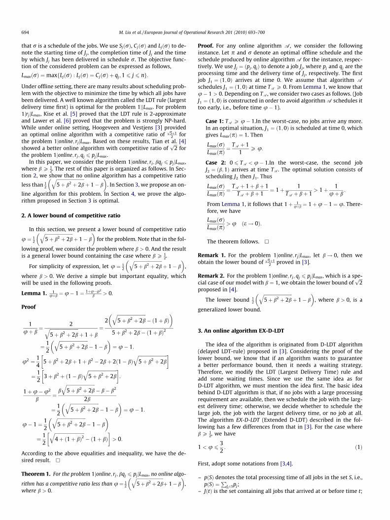
Proof. By contradiction. Suppose that r consists of more than oneblock (see Fig. 1). Let B be the block that contains job Jl,

LlðrÞ ¼ LmaxðrÞ: ð2Þ

(1) The first step is to reduce the jobs’ number of the small-est counterexample by its definition.Consider any block that precedes B. Since the algorithmbases its choices on the set ðJðtÞ n Jðt1ÞÞ

SUðt1Þ (consider-

ing the definition of the big job), the existence of the jobsthat are completed before the start of block B does notinfluence the start time of B and the order in which thejobs are executed. Therefore, we delete all jobs com-pleted before the start of block B without changing thevalue LmaxðrÞ and increasing LmaxðpÞ. Similarly, we canremove all jobs from I that are released after the starttime SlðrÞ of Jl in r.

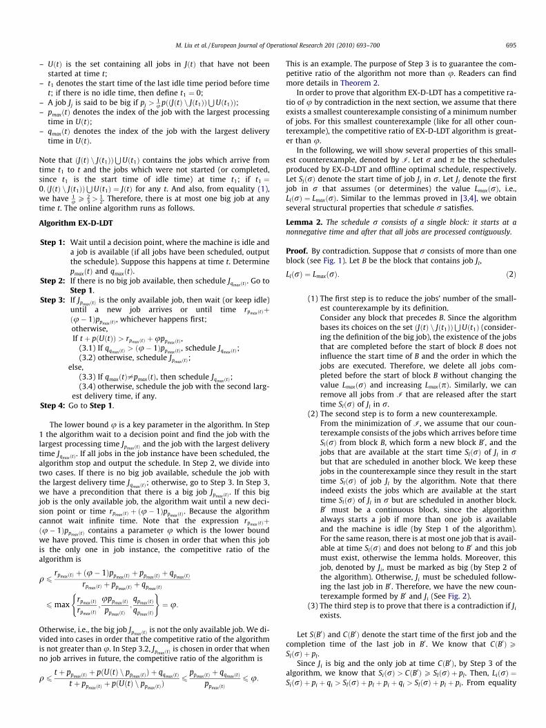
(2) The second step is to form a new counterexample.From the minimization of I, we assume that our coun-terexample consists of the jobs which arrives before timeSlðrÞ from block B, which form a new block B0, and thejobs that are available at the start time SlðrÞ of Jl in rbut that are scheduled in another block. We keep thesejobs in the counterexample since they result in the starttime SlðrÞ of job Jl by the algorithm. Note that thereindeed exists the jobs which are available at the starttime SlðrÞ of Jl in r but are scheduled in another block.B0 must be a continuous block, since the algorithmalways starts a job if more than one job is availableand the machine is idle (by Step 1 of the algorithm).For the same reason, there is at most one job that is avail-able at time SlðrÞ and does not belong to B0 and this jobmust exist, otherwise the lemma holds. Moreover, thisjob, denoted by Ji, must be marked as big (by Step 2 ofthe algorithm). Otherwise, Ji must be scheduled follow-ing the last job in B0. Therefore, we have the new coun-terexample formed by B0 and Ji (See Fig. 2).

(3) The third step is to prove that there is a contradiction if Ji

exists.

Let SðB0Þ and CðB0Þ denote the start time of the first job and thecompletion time of the last job in B0. We know that CðB0ÞPSlðrÞ þ pl.

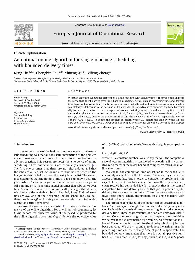
Since Ji is big and the only job at time CðB0Þ, by Step 3 of thealgorithm, we know that SiðrÞ > CðB0ÞP SlðrÞ þ pl. Then, LiðrÞ ¼SiðrÞ þ pi þ qi > SlðrÞ þ pl þ pi þ qi > SlðrÞ þ pl þ pi. From equality

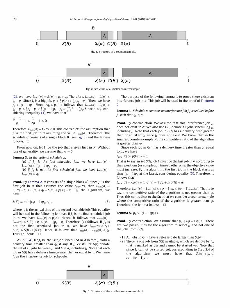
Fig. 1. Structure of a counterexample.

Fig. 2. Structure of a smaller counterexample.


(2), we have LmaxðrÞ ¼ SlðrÞ þ pl þ ql. Therefore, LmaxðrÞ � LiðrÞ <ql � pi. Since Ji is a big job, pi >

1u pðIÞ > 1

u ðpi þ plÞ. Then, we havepl < ðu� 1Þpi. Since bql 6 pl, it follows that LmaxðrÞ � LiðrÞ <ql � pi 6

1b pl � pi <

1b ðu� 1Þpi � pi ¼

u�1b � 1

� �pi. Since b P 1

2, con-sidering inequality (1), we have that

u� 1b� 1 6

12b� 1 6 0:

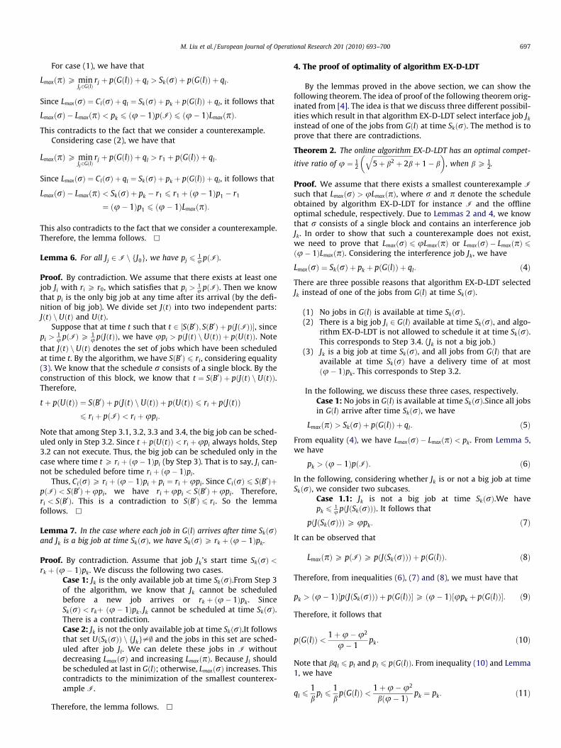
Therefore, LmaxðrÞ � LiðrÞ < 0. This contradicts the assumption thatJl is the first job in r assuming the value LmaxðrÞ. Therefore, Theschedule r consists of a single block B0 (see Fig. 3) and the lemmafollows. h

From now on, let J0 be the job that arrives first in I. Withoutloss of generality, we assume that r0 ¼ 0.

Lemma 3. In the optimal schedule p,
(a) if J0 is the first scheduled job, we have LmaxðrÞ�LmaxðpÞ 6 ðu� 1Þp0 þ ql;(b) if J0 is not the first scheduled job, we have LmaxðrÞ�LmaxðpÞ 6 ql.
Proof. By Lemma 2, r consists of a single block B0. Since Jl is thefirst job in r that assumes the value LmaxðrÞ, then LmaxðrÞ ¼ClðrÞ þ ql 6 CðB0Þ þ ql ¼ SðB0Þ þ pðIÞ þ ql. By the algorithm, wehave

SðB0Þ ¼minfðu� 1Þp0; r1g; ð3Þ

where r1 is the arrival time of the second available job. This equalitywill be used in the following lemmas. If J0 is the first scheduled jobin p, we have LmaxðpÞP pðIÞ. Hence, it follows that LmaxðrÞ�LmaxðpÞ 6 SðB0Þ þ ql 6 ðu� 1Þp0 þ ql. Therefore, (a) follows. If J0 isnot the first scheduled job in p, we have LmaxðpÞP r1þpðIÞP SðB0Þ þ pðIÞ. Hence, it follows that LmaxðrÞ � LmaxðpÞ 6 ql.Thus, (b) holds. h

As in [3,4], let Jk be the last job scheduled in r before Jl with adelivery time smaller than ql, if any. If Jk exists, let GðlÞ denotethe set of all jobs between Jk and Jl in r, including Jl. Note that eachjob in GðlÞ has a delivery time greater than or equal to ql. We nameJk as the interference job for schedule.

Fig. 3. Structure of the smal

The purpose of the following lemma is to prove there exists aninterference job in r. This job will be used in the proof of Theorem2.

Lemma 4. Schedule r contains an interference job Jk scheduled beforeJl such that qk 6 ql.

Proof. By contradiction. We assume that this interference job Jk

does not exist in r. We also use GðlÞ denote all jobs scheduling Jl,including Jl. Note that each job in GðlÞ has a delivery time greaterthan or equal to ql since Jk does not exist. We know that in thesmallest counterexample I, the competitive ratio of the algorithmis greater than u.

Since each job in GðlÞ has a delivery time greater than or equalto ql, we have

LmaxðpÞP pðGðlÞÞ þ ql:

That is to say, in set GðlÞ, job Jl must be the last job in r according totheir positions (or completion times); otherwise, the objective valuemust increase. By the algorithm, the first job in the block starts attime ðu� 1Þp0 at the latest, considering equality (3). Therefore, itfollows that

LmaxðrÞ ¼ ClðrÞ þ ql 6 ðu� 1Þp0 þ pðGðlÞÞ þ ql:

Therefore, LmaxðrÞ � LmaxðpÞ 6 ðu� 1Þp0 6 ðu� 1ÞLmaxðpÞ. That is tosay, the competitive ratio of the algorithm is not greater than u.Thus, this contradicts to the fact that we consider a counterexamplewhere the competitive ratio of the algorithm is greater than u.Therefore, the lemma follows. h

Lemma 5. pk > ðu� 1ÞpðIÞ.

Proof. By contradiction. We assume that pk 6 ðu� 1ÞpðIÞ. Thereare two possibilities for the algorithm to select Jk and not one ofthe jobs from GðlÞ.

(1) All jobs in GðlÞ have a release date larger than SkðrÞ.(2) There is one job from GðlÞ available, which we denote by J1,

that is marked as big and cannot be started yet. Note thatsince J1 cannot be started yet, corresponding to Step 3.4 ofthe algorithm, we must have that SkðrÞ þ pk 6

r1 þ ðu� 1Þp1.

lest counterexample I.


For case (1), we have that

LmaxðpÞP minJj2GðlÞ

rj þ pðGðlÞÞ þ ql > SkðrÞ þ pðGðlÞÞ þ ql:

Since LmaxðrÞ ¼ ClðrÞ þ ql ¼ SkðrÞ þ pk þ pðGðlÞÞ þ ql, it follows that

LmaxðrÞ � LmaxðpÞ < pk 6 ðu� 1ÞpðIÞ 6 ðu� 1ÞLmaxðpÞ:

This contradicts to the fact that we consider a counterexample.Considering case (2), we have that

LmaxðpÞP minJj2GðlÞ

rj þ pðGðlÞÞ þ ql > r1 þ pðGðlÞÞ þ ql:

Since LmaxðrÞ ¼ ClðrÞ þ ql ¼ SkðrÞ þ pk þ pðGðlÞÞ þ ql, it follows that

LmaxðrÞ � LmaxðpÞ < SkðrÞ þ pk � r1 6 r1 þ ðu� 1Þp1 � r1

¼ ðu� 1Þp1 6 ðu� 1ÞLmaxðpÞ:

This also contradicts to the fact that we consider a counterexample.Therefore, the lemma follows. h

Lemma 6. For all Jj 2 I n fJ0g, we have pj 61u pðIÞ.

Proof. By contradiction. We assume that there exists at least onejob Ji with ri P r0, which satisfies that pi >

1u pðIÞ. Then we know

that pi is the only big job at any time after its arrival (by the defi-nition of big job). We divide set JðtÞ into two independent parts:JðtÞ n UðtÞ and UðtÞ.

Suppose that at time t such that t 2 ½SðB0Þ; SðB0Þ þ pðJðIÞÞ�, sincepi >

1u pðIÞP 1

u pðJðtÞÞ, we have upi > pðJðtÞ n UðtÞÞ þ pðUðtÞÞ. Note

that JðtÞ n UðtÞ denotes the set of jobs which have been scheduledat time t. By the algorithm, we have SðB0Þ 6 ri, considering equality(3). We know that the schedule r consists of a single block. By theconstruction of this block, we know that t ¼ SðB0Þ þ pðJðtÞ n UðtÞÞ.Therefore,

t þ pðUðtÞÞ ¼ SðB0Þ þ pðJðtÞ n UðtÞÞ þ pðUðtÞÞ 6 ri þ pðJðtÞÞ6 ri þ pðIÞ < ri þupi:

Note that among Step 3.1, 3.2, 3.3 and 3.4, the big job can be sched-uled only in Step 3.2. Since t þ pðUðtÞÞ < ri þupi always holds, Step3.2 can not execute. Thus, the big job can be scheduled only in thecase where time t P ri þ ðu� 1Þpi (by Step 3). That is to say, Ji can-not be scheduled before time ri þ ðu� 1Þpi.

Thus, CiðrÞP ri þ ðu� 1Þpi þ pi ¼ ri þupi. Since CiðrÞ 6 SðB0ÞþpðIÞ < SðB0Þ þupi, we have ri þupi < SðB0Þ þupi. Therefore,ri < SðB0Þ. This is a contradiction to SðB0Þ 6 ri. So the lemmafollows. h

Lemma 7. In the case where each job in GðlÞ arrives after time SkðrÞand Jk is a big job at time SkðrÞ, we have SkðrÞP rk þ ðu� 1Þpk.

Proof. By contradiction. Assume that job Jk’s start time SkðrÞ <rk þ ðu� 1Þpk. We discuss the following two cases.

Case 1: Jk is the only available job at time SkðrÞ.From Step 3of the algorithm, we know that Jk cannot be scheduledbefore a new job arrives or rk þ ðu� 1Þpk. SinceSkðrÞ < rkþ ðu� 1Þpk; Jk cannot be scheduled at time SkðrÞ.There is a contradiction.Case 2: Jk is not the only available job at time SkðrÞ.It followsthat set UðSkðrÞÞ n fJkg–; and the jobs in this set are sched-uled after job Jl. We can delete these jobs in I withoutdecreasing LmaxðrÞ and increasing LmaxðpÞ. Because Jl shouldbe scheduled at last in GðlÞ; otherwise, LmaxðrÞ increases. Thiscontradicts to the minimization of the smallest counterex-ample I.

Therefore, the lemma follows. h

4. The proof of optimality of algorithm EX-D-LDT

By the lemmas proved in the above section, we can show thefollowing theorem. The idea of proof of the following theorem orig-inated from [4]. The idea is that we discuss three different possibil-ities which result in that algorithm EX-D-LDT select interface job Jk

instead of one of the jobs from GðlÞ at time SkðrÞ. The method is toprove that there are contradictions.

Theorem 2. The online algorithm EX-D-LDT has an optimal compet-

itive ratio of u ¼ 12


qþ 1� b

� �, when b P 1

2.

Proof. We assume that there exists a smallest counterexample I

such that LmaxðrÞ > uLmaxðpÞ, where r and p denote the scheduleobtained by algorithm EX-D-LDT for instance I and the offlineoptimal schedule, respectively. Due to Lemmas 2 and 4, we knowthat r consists of a single block and contains an interference jobJk. In order to show that such a counterexample does not exist,we need to prove that LmaxðrÞ 6 uLmaxðpÞ or LmaxðrÞ � LmaxðpÞ 6ðu� 1ÞLmaxðpÞ. Considering the interference job Jk, we have

LmaxðrÞ ¼ SkðrÞ þ pk þ pðGðlÞÞ þ ql: ð4Þ

There are three possible reasons that algorithm EX-D-LDT selectedJk instead of one of the jobs from GðlÞ at time SkðrÞ.

(1) No jobs in GðlÞ is available at time SkðrÞ.(2) There is a big job Ji 2 GðlÞ available at time SkðrÞ, and algo-

rithm EX-D-LDT is not allowed to schedule it at time SkðrÞ.This corresponds to Step 3.4. (Jk is not a big job.)

(3) Jk is a big job at time SkðrÞ, and all jobs from GðlÞ that areavailable at time SkðrÞ have a delivery time of at mostðu� 1Þpk. This corresponds to Step 3.2.

In the following, we discuss these three cases, respectively.
Case 1: No jobs in GðlÞ is available at time SkðrÞ.Since all jobsin GðlÞ arrive after time SkðrÞ, we have
LmaxðpÞ > SkðrÞ þ pðGðlÞÞ þ ql: ð5Þ

From equality (4), we have LmaxðrÞ � LmaxðpÞ < pk. From Lemma 5,we have

pk > ðu� 1ÞpðIÞ: ð6Þ

In the following, considering whether Jk is or not a big job at timeSkðrÞ, we consider two subcases.

Case 1.1: Jk is not a big job at time SkðrÞ.We havepk 6

1u pðJðSkðrÞÞÞ. It follows that

pðJðSkðrÞÞÞP upk: ð7Þ

It can be observed that

LmaxðpÞP pðIÞP pðJðSkðrÞÞÞ þ pðGðlÞÞ: ð8Þ

Therefore, from inequalities (6), (7) and (8), we must have that

pk > ðu� 1Þ½pðJðSkðrÞÞÞ þ pðGðlÞÞ�P ðu� 1Þ½upk þ pðGðlÞÞ�: ð9Þ

Therefore, it follows that

pðGðlÞÞ < 1þu�u2

u� 1pk: ð10Þ

Note that bql 6 pl and pl 6 pðGðlÞÞ. From inequality (10) and Lemma1, we have

ql 61b

pl 61b

pðGðlÞÞ < 1þu�u2

bðu� 1Þ pk ¼ pk: ð11Þ


We distinguish two possibilities according to where J0 is scheduledin p.

Case 1.1.1: J0 is not the first scheduled job in p.By Lemma 3,we have LmaxðrÞ � LmaxðpÞ 6 ql. From inequalities (7), (8) and(11) and Lemma 1, it follows that

LmaxðrÞ � LmaxðpÞLmaxðpÞ

6ql

pðJððSkðrÞÞÞÞ þ pðGðlÞÞ 6ql

upk þ bql<

1uþ b

¼ u� 1:

Case 1.1.2: J0 is the first scheduled job in p.We use BkðrÞ todenote the set of jobs which arrive at or before time SkðrÞand are scheduled before job Jk in r. Let AlðrÞ denote theset of jobs which arrive at or before time SkðrÞ and arescheduled after job Jl in r. Then we can divide JðSkðrÞÞ into3 parts, BkðrÞ; pk;AlðrÞ. Therefore, we know

SkðrÞ ¼ SðB0Þ þ pðBkðrÞÞ: ð12Þ

and JðSkðrÞÞ ¼ BkðrÞS

Jk

SAlðrÞ, which deduces that

pðJkðrÞÞ ¼ pðBkðrÞÞ þ pk þ pðAlðrÞÞ: ð13Þ

Note that BkðrÞ and AlðrÞ may be empty. Then pðBkðrÞÞP 0 andPðAlðrÞÞP 0. We will consider two subcases divided by whetherJk is scheduled after all jobs in GðlÞ in p or not.

Case 1.1.2.1: Jk is not scheduled after all jobs in GðlÞ in p.Con-sidering that SðB0Þ ¼ fðu� 1Þp0; r1g, where r1 is the arrivaltime of the second available job, we have

SðB0Þ 6 ðu� 1Þp0: ð14Þ

Since it is possible that Jk � J0, we further discuss the following twosubcases.

Subcase 1: Jk–J0.It follows that BkðrÞmust contain J0. There-fore, pðBkðrÞÞP p0. Then we have

LmaxðpÞP p0 þ pk þ pðGðlÞÞ þ ql P p0 þ pk þ pl þ ql: ð15Þ

Considering equality (4) and inequality (8), we have

LmaxðrÞ � LmaxðpÞ 6 SkðrÞ þ pk þ ql � pðJkðrÞÞ:

From equalities (12) and (13), it follows that

LmaxðrÞ � LmaxðpÞ 6 SðB0Þ þ ql � pðAlðrÞÞ 6 SðB0Þ þ ql: ð16Þ

Therefore, from inequalities (16) and (14), we have

LmaxðrÞ � LmaxðpÞ 6 ðu� 1Þp0 þ ql: ð17Þ

Considering inequalities (15), we have


6ðu� 1Þp0 þ ql

p0 þ pk þ pl þ ql6 max u� 1;

ql

pk þ pl þ ql

:

From inequalities (1) and (11) and Lemma 1, it follows that

ql

pk þ pl þ ql<

12þ b

<1

uþ b¼ u� 1:

Therefore, we have


6 u� 1:

Subcase 2: Jk ¼ J0.In this case Jk is the first job in r, we haveBkðrÞ ¼ ; and SkðrÞ ¼ SðB0Þ. Considering inequality (14), itfollows that SkðrÞ 6 ðu� 1Þp0. From equality (4) andLmaxðpÞP pk þ pðGðlÞÞ þ ql, we have

LmaxðrÞ � LmaxðpÞ 6 SkðrÞ 6 ðu� 1Þp0 < ðu� 1ÞLmaxðpÞ:

Case 1.1.2.2: Jk is scheduled after all jobs in GðlÞ in p.Wehave

LmaxðpÞ > SkðrÞ þ pðGðlÞÞ þ pk þ qk: ð18Þ

Since Jk is not a big job, we have

pðJðSkðrÞÞÞP upk: ð19Þ

Considering equality (4) and inequality (18), we haveLmaxðrÞ � LmaxðpÞ < ql � qk 6 ql: ð20ÞFrom inequalities (8), (11), (19) and (20) and Lemma 1, it followsthat


<ql

pðJðSkðrÞÞÞ þ pðGðlÞÞ <ql

upk þ bql<

1uþ b

¼ u� 1:

Case 1.2: Jk is a big job at time SkðrÞ.From Lemma 7, we have

SkðrÞP rk þ ðu� 1Þpk P ðu� 1Þpk: ð21Þ

We consider the following two subcases divided by whether Jk isscheduled after all jobs in GðlÞ in p or not.

Case 1.2.1: Jk is scheduled after all jobs in GðlÞ in p.If ql P pk,from inequality (5), we have

LmaxðpÞ > SkðrÞ þ pðGðlÞÞ þ ql P SkðrÞ þ pl þ ql

¼ SkðrÞ þ ðbþ 1Þql P SkðrÞ þ ðbþ 1Þpk: ð22Þ

From equality (4), inequalities (5), (21) and (22) and Lemma 1, wehave


<pk

SkðrÞ þ ðbþ 1Þpk6

pk

ðuþ bÞpk¼ u� 1:

Otherwise, i.e., ql < pk. Then we have

LmaxðpÞ > SkðrÞ þ pðGðlÞÞ þ pk þ qk: ð23Þ

From Eq. (4), inequalities (11), (21) and (23), and Lemma 1, it fol-lows that,


<ql � qk

SkðrÞ þ pðGðlÞÞ þ pk þ qk6

ql

SkðrÞ þ pl þ pk

<ql

upk þ pl<

1uþ b

¼ u� 1:

Case 1.2.2: Jk is not scheduled after all jobs in GðlÞ in p.Recallthe definition of BkðrÞ, we have BkðrÞ

SfJkg ¼ UðJðSkðrÞÞÞ.

We know that

LmaxðpÞP pk þ pðGðlÞÞ þ ql: ð24Þ

If BkðrÞ ¼ ;, we know

SkðrÞ ¼ rk þ ðu� 1Þpk: ð25Þ

Considering that Jk is not scheduled after all jobs in GðlÞ in p, weknow that Jl must be scheduled at last in the set GðlÞ

SJk in p.If Jk

is scheduled before all jobs in GðlÞ in p, we have LmaxðpÞPrk þ pk þ pðGðlÞÞ þ ql. Otherwise, i.e., if Jk is not scheduled beforeall jobs in GðlÞ in p, there must be LmaxðpÞ > rk þ pkþpðGðlÞÞ þ ql.Considering above two situations, we have

LmaxðpÞ > rk þ pk þ pðGðlÞÞ þ ql: ð26Þ

From equalities (4) and (25) and inequality (26), it follows that

LmaxðrÞ � LmaxðpÞ 6 SkðrÞ � rk ¼ ðu� 1Þpk < ðu� 1ÞLmaxðpÞ:

Then, we suppose that BkðrÞ–;. So we have that Jk–J0. Let Ji be thejob completed at time SkðrÞ in r. So we have

SkðrÞ ¼ SiðrÞ þ pi: ð27Þ

It follows that

LmaxðrÞ ¼ SiðrÞ þ pi þ pk þ pðGðlÞÞ þ ql: ð28Þ


Since Jk is big, from equality (13), we have upk > pðBkðrÞÞþpk þ pðAlðrÞÞ. It follows that

pðBkðrÞÞ < ðu� 1Þpk � pðAlðrÞÞ 6 ðu� 1Þpk: ð29Þ

We consider two possibilities distinguished by whether rk 6 SiðrÞor not.

Case 1.2.2.1: rk 6 SiðrÞ.From inequality (21) and equality(27), we have SiðrÞ þ pi P rk þ ðu� 1Þpk. Therefore,SiðrÞ þ piþ pk P rk þupk. If SkðrÞ ¼ rk þ ðu� 1Þpk, fromequality (4) and inequality (26), we have


6SkðrÞ � rk

rk þ pk þ pðGðlÞÞ þ ql<ðu� 1Þpk

pk¼ u� 1:

Then we consider the case where SkðrÞ > rk þ ðu� 1Þpk. By thealgorithm, Step 3.1 must occur at time SiðrÞ. Therefore, we have

qi > ðu� 1Þpk: ð30Þ

Then we consider the following two subcases divided by whether Ji

is scheduled after all jobs in GðlÞ in p or not.
Subcase 1: Ji is scheduled after all jobs in GðlÞ in p.SinceBkðrÞ–;, we know that J0–Jk. It follows that
rk P SðB0Þ ð31Þ

and that

SkðrÞ ¼ SðB0Þ þ pðBkðrÞÞ: ð32Þ

In this subcase, Ji is scheduled after all jobs in the set GðlÞS

Jk in p.Considering that Jk is not scheduled after all jobs in GðlÞ in p, weknow that Jl must be scheduled at last in the set GðlÞ

SJk in p. If

pi þ qi P ql, we have LmaxðpÞP rk þ pk þ pðGðlÞÞ þ pi þ qi. Otherwise,if pi þ qi < ql, we have LmaxðpÞP rk þ pk þ pðGðlÞÞ þ ql. Therefore, wehave

LmaxðpÞP rk þ pk þ pðGðlÞÞ þmaxfpi þ qi; qlg: ð33Þ

From equalities (4) and (32), we know

LmaxðrÞ ¼ SðB0Þ þ pðBkðrÞÞ þ pk þ pðGðlÞÞ þ ql: ð34Þ

From inequalities (31) and (33) and equality (34), it follows that

LmaxðrÞ � LmaxðpÞ 6 pðBkðrÞÞ þ ql � pi � qi þ ðSðB0Þ � rkÞ6 pðBkðrÞÞ þ ql � pi � qi: ð35Þ

Considering inequality (30) and pi P bqi, we have

pi > bðu� 1Þpk: ð36Þ

From inequalities (29), (30), (35) and (36), we have

LmaxðrÞ � LmaxðpÞ < ðu� 1Þpk þ ql � bðu� 1Þpk � ðu� 1Þpk

¼ ql � bðu� 1Þpk < ql: ð37Þ

From inequality (24), we know LmaxðpÞP pk þ pðGðlÞÞþql P pk þ pl þ ql P pk þ ðbþ 1Þql. Since I is a counterexample, wemust have

ql > ðu� 1ÞLmaxðpÞP ðu� 1Þpk þ ðu� 1Þðbþ 1Þql: ð38Þ

Therefore, Considering Lemma 1, we have

pk <1

u� 1� b� 1

� �ql ¼ ðuþ b� b� 1Þql ¼ ðu� 1Þql: ð39Þ

From equality (4) and inequalities (5) and (39), we have

LmaxðrÞ � LmaxðpÞ < pk < ðu� 1Þql < ðu� 1ÞLmaxðpÞ:

Subcase 2: Ji is not scheduled after all job in GðlÞ in p.Wehave

LmaxðpÞP pk þ pi þ pðGðlÞÞ þ ql: ð40Þ

Since BkðrÞ–;, we know that J0–Jk. It follows that

LmaxðrÞ ¼ SðB0Þ þ pðBkðrÞÞ þ pk þ pðGðlÞÞ þ ql ð41Þ

and that

LmaxðpÞ > p0 þ pk: ð42Þ

From inequalities (40) and (41), we have

LmaxðrÞ � LmaxðpÞ 6 SðB0Þ þ pðBkðrÞÞ � pi 6 SðB0Þ þ pðBkðrÞÞ: ð43Þ

Since SðB0Þ ¼ minfðu� 1Þp0; r1g, we have

SðB0Þ 6 ðu� 1Þp0: ð44Þ

From inequalities (29), (42), (43) and (44), it follows that

LmaxðrÞ � LmaxðpÞ < ðu� 1Þp0 þ ðu� 1Þpk < ðu� 1Þðp0 þ pkÞ< ðu� 1ÞLmaxðpÞ:

Case 1.2.2.2: rk > SiðrÞ.We know that

LmaxðpÞP rk þ pk þ pðGðlÞÞ þ ql: ð45Þ

From equality (28) and inequality (45), we have

LmaxðrÞ � LmaxðpÞ 6 SiðrÞ þ pi � rk < pi 6 pðBkðrÞÞ: ð46Þ

From inequalities (29) and (46), it follows that

LmaxðrÞ � LmaxðpÞ < pðBkðrÞÞ < ðu� 1Þpk < ðu� 1ÞLmaxðpÞ:

Case 2: There is a big job Ji 2 GðlÞ available at time SkðrÞ andalgorithm EX-D-LDT is not allowed to schedule it at timeSkðrÞ. This corresponds to Step 3.4. (Jk is not a big job.)Weclaim that Ji must be the only job from GðlÞ available at timeSkðrÞ. Suppose to the contrary that there is another job Jj

from GðlÞ except Ji available at time SkðrÞ. According to thedefinition of GðlÞ, we have qk < minfqi; qjg. By Step 3.3 and3.4 of the algorithm, Jk must not be selected to schedule attime SkðrÞ. There is a contradiction. Therefore, we have that

LmaxðpÞP ri þ pðGðlÞÞ þ ql: ð47Þ

By the above claim, we know that Ji is both the job with largestdelivery time and the job with largest processing time at timeSkðrÞ. So, we know the index pmaxðSkðrÞÞ ¼ qmaxðSkðrÞÞ. Therefore,Step 3.4 of the algorithm must occur at time SkðrÞ. This implies thatSkðrÞ þ pk þ pi 6 ri þupi. Therefore, we have

SkðrÞ þ pk 6 ri þ ðu� 1Þpi: ð48Þ

From equality (4) and inequalities (47) and (48) we have

LmaxðrÞ � LmaxðpÞ 6 SkðrÞ þ pk � ri 6 ri þ ðu� 1Þpi � ri

¼ ðu� 1Þpi 6 ðu� 1ÞLmaxðpÞ:

Case 3: Jk is a big job at time SkðrÞ, and all of the jobs fromGðlÞ that are available at time SkðrÞ have a delivery time ofat most ðu� 1Þpk. This corresponds to Step 3.2.Since Jl isthe job with minimum delivery time in GðlÞ, we have

ql 6 ðu� 1Þpk: ð49Þ

Consider the following two cases.
Case 3.1: J0 is not the first job in p.From Lemma 3 andinequality (49), we have that
LmaxðrÞ � LmaxðpÞ 6 ql 6 ðu� 1Þpk < ðu� 1ÞLmaxðpÞ:

Case 3.2: J0 is the first job in p.From Lemma 3 and inequality(49), we have

LmaxðrÞ � LmaxðpÞ 6 ðu� 1Þp0 þ ql 6 ðu� 1Þðp0 þ pkÞ: ð50Þ


If J0–Jk, we have LmaxðpÞ > p0 þ pk. Therefore, from inequality (50), itfollows that

LmaxðrÞ � LmaxðpÞ 6 ðu� 1Þðp0 þ pkÞ < ðu� 1ÞLmaxðpÞ:

If J0 ¼ Jk, then Jk is the first job in p. therefore, we have

LmaxðpÞP pk þ pðGðlÞÞ þ ql: ð51Þ

Therefore, from equality (4), we have

LmaxðrÞ � LmaxðpÞ 6 SkðrÞ: ð52Þ

Since I is a counterexample, we must have SkðrÞ > ðu� 1Þpk. (Notethat rk ¼ 0.) This implies that the algorithm must run Step 3.1 atleast once. Let T be the starting time of the first job completed aftertime ðu� 1Þpk. Let Q denote the set of jobs processed from time T totime SkðrÞ in r. So we know that

T 6 ðu� 1Þpk ð53Þ

and QT

GðlÞ ¼ ;. Since Jk is a big job and the jobs in Q are scheduledbefore Jk in r, from Step 3.1, we have that each job in Q has a deliv-ery time more than ðu� 1Þpk. From inequality (49), ql 6 ðu� 1Þpk,we know that each job in Q

SGðlÞ has a delivery time at least ql.

Therefore, we have

LmaxðpÞP pk þ pðQÞ þ pðGðlÞÞ þ minJj2QS

GðlÞqj

¼ pk þ pðQÞ þ pðGðlÞÞ þ ql: ð54Þ

We also know that

LmaxðrÞ ¼ T þ pðQÞ þ pk þ pðGðlÞÞ þ ql: ð55Þ

From equalities (53)–(55), it follows that

LmaxðrÞ � LmaxðpÞ 6 T 6 ðu� 1Þpk < ðu� 1ÞLmaxðpÞ:

The theorem follows. h

Acknowledgements

The authors would like to acknowledge the constructive com-ments by anonymous referees which have improved the presenta-tion of the paper. This work is partially supported by NSF of Chinaunder Grants 70525004, 60736027 and 70702030.

References

[1] A. Borodin, R. El-Yaniv, Online Computation and Competitive Analysis,Cambridge University Press, Cambridge, 1998.

[2] K. Pruhs, J. Sgall, E. Torng, Online scheduling, in: J.Y.-T. Leung (Ed.), Handbook ofScheduling: Algorithms, Models, and Performance Analysis, 2004.

[3] J.A. Hoogeveen, A.P.A. Vestjens, A best possible deterministic on-line algorithmfor minimizing maximum delivery time on a single machine, SIAM Journal onDiscrete Mathematics 13 (2000) 56–63.

[4] Ji Tian, Ruyan Fu, Jinjiang Yuan, A best on-line algorithm for single machinescheduling with small delivery times, Theoretical Computer Science 393 (2008)287–293.

[5] H. Kise, T. Iberaki, H. Mine, Performance analysis of six approximationalgorithms for the one-machine maximum lateness scheduling problem withready times, Journal of Operation Research Society Japan 22 (1979) 205–224.

[6] E.L. Lawler, J.K. Lenstra, A.H.G. Rinnooy Kan, D.B. Shmoys, Sequencing andscheduling: Algorithms and complexity, in: S.C. Graves, P.H. Zipkin, A.H.G.Rinnooy Kan (Eds.), Logistics of Production and Inventory, Handbooks ofOperation Research Management Science, vol. 4, North-Holland, Amsterdam,1993, pp. 445–522.

Documents

An optimal online algorithm for single machine scheduling with bounded delivery times