ANALYSIS OF APERTURE ANTENNAS

IN INHOMOGENEOUS ~ffiDIA

by

Dikran Damlamayan

Antenna Laboratory

Technical Report No. 52

This research was supported by the

U. S. Air Force through the Air Force.

CALIFORNIA INSTITUTE OF TECHNOLOGY

Pasadena, California

November 1969

-ii-

ACKNOWLEDGEMENT

I wish to express my sincere gratitude to my research advisor

Professor Charles Herach Papas, for his continued gUidance and support

during the course of this work, as well as for the unceasing encourage­

ment and deep inspiration I received from him throughout my studies at

the California Institute of Technology.

I acknowledge with thanks the assistance of Miss Kikuko Matsumoto

in computer programming, and the efforts of Mrs. Carol Teeter in typing

the final manuscript.

I also wish to thank Dr. Henri Hodara of Tetra Tech for his

enthusiasm and interest in this work.

-iii-

ABSTRACT

The object of this report is to calculate the admittance and

the radiation pattern of aperture antennas fed by waveguides of arbitrary

cross-section and radiating into dielectric slabs, whose constitutive

parameters may be functions of position along the direction normal to

the slab faces.

For a given aperture field distribution the antenna aperture

admittance and the radiation field are expressed here, for the first

time, in terms of two auxiliary quantities directly related to the plane

wave reflection and transmission coefficients of the dielectric slab.

These quantities are the input admittance of the dielectric slab and the

ratio of the total electric field amplitude transmitted at one end of

the slab to the transverse field at the other, both calculated for plane

waves as a function of incident propagation direction. This approach

introduces a great simplification in the solution of the problem,

particularly in the case of an antenna radiating into an inhomogeneous

dielectric slab.

A simple and powerful method has been devised for the computa­

tion of the input admittance of an inhomogeneous dielectric slab as well

as for the electric field ratio. In this case the impracticability of

obtaining analytical results has necessitated the use of numerical

techniques.

Examples of the application of the theory to typical dielec­

tric slabs are given and the results are discussed.

-iv-

TABLE OF CONTENTS

1. INTRODUCTION 1

2. VARIATIONAL TREATMENT OF WAVEGUIDE-FED APERTURE ADMITTANCE 7

3. APERTURE ANTENNA CHARACTERISTICS 16

A. Plane Wave Synthesis of Aperture Distributions 16

B. Aperture Admittance 24

C. Radiation Pattern 39

4. REFLECTION AND TRANSMISSION PROPERTIES OF INHOMOGENEOUS

DIELECTRIC SLABS 46

A. Perpendicular Polarization 48

B. Parallel Polarization 56

5. RESULTS AND CONCLUSIONS 68

REFERENCES 84

-1-

1. INTRODUCTION

The study of antennas covered by dielectrics has been of

particular interest to scientists and engineers in the last decade.

Interest in this problem is generated because of two situations of

practical importance that scientists have been confronted with. The

first arises in connection with maintaining radio communication with

space vehicles at reentry. High speed space vehicles reentering the

earth's atmosphere are surrounded by an ionized gas layer or a plasma

sheath which strongly affects the propagation of electromagnetic waves.

The presence of the plasma sheath causes a mismatch between transmitter

or receiver and the antenna, and a distortion of the antenna radiation

pattern, thus creating problems in the maintenance of radio communi­

cation between the vehicle and ground stations. As a result, the study

of the admittance and the radiation pattern of an antenna covered by

plasma sheaths of varying properties is of primary importance. The

second situation arises in connection with plasma diagnostics. Elec­

tromagnetic waves in plasma make it possible to extract information

about such plasma characteristics as electron densities or relaxation

times. Often the first step in the measurement of these properties is

the determination of the admittance of an antenna in the plasma.

This report presents a new and simple method for the calcula­

tion of the admittance and radiation pattern of antennas consisting of

waveguide-fed apertures in infinitely conducting ground planes, and

radiating into dielectric slabs of varying properties. The usefulness

-2-

and simplicity of the method stern from the fact that the usual boundary­

value problem approach, involving lengthy calculations for each special

situation, is bypassed.

As is well known, for each of the two independent polarization

directions of an incident plane wave and as a function of its propagation

direction, a dielectric slab has a reflection coefficient and a trans­

mission coefficient. Given the aperture field distribution, the ex­

pression for the aperture admittance of the antenna is shown to involve

these reflection coefficients or equivalently the input admittances of

the slab. Similarly the slab transmission coefficients enter into the

expression for the radiation field. The problem is formulated in such

a way that it can readily be applied for any aperture shape and corres­

ponding waveguide cross-section. In most instances we are interested

in infinite slots and circular, annular or rectangular apertures in

flat ground planes. Hence, we will be concerned particularly with these

configurations.

Furthermore the expressions derived are valid for any kind of

dielectric medium of practical interest making up the slab - homogeneous,

inhomogeneous or turbulent with constitutive parameters varying only

along the direction normal to the slab faces. The present method is

particularly useful for slabs which are not homogeneous isotropic media,

since the difficulty involved in these cases is reduced to the calcula­

tion of the appropriate reflection and transmission coefficients which

then are used in the evaluation of antenna admittance and radiation

field.

-3-

Antennas in lossy, dielectric media have been the subject of

many studies for almost half a century. However since this report deals

essentially with the admittance and radiation pattern of radiating

apertures, only those investigations which have some bearing on the

present problem will be mentioned here.

Levine and SChwlL!ger (1,2) starting with integral equation,

formulations, have arrived for the first time at variational expressions

for the far field from an aperture in an infinite plane screen on which

a plane scalar or electromagnetic wave is incident. Levine and Papas (3)

in a similar way have found variational expressions for the admittance

of an annular aperture in an infinite plane conducting screen fed by a

coaxial waveguide and radiating into free space. Using similar techniques

Lewin (4) has calculated the admittance of a rectangular waveguide-fed

aperture radiating into free space.

Variational techniques have consistently been used in the

calculation of the admittance of dielectric covered waveguide-fed slots

as well. In almost all cases the fields everywhere are expressed in

terms of their Fourier transforms and the boundary-value problem is

solved assuming the aperture field to consist of the dominant waveguide

mode. The admittance of a rectangular waveguide-fed slot covered by a

homogeneous plasma layer has been calculated by Galejs (5). However his

formulation is quite involved and does not apply to plasma layers whose

thickness is small compared to a wavelength. Galejs (6,7) has also

computed the admittance of plasma-covered annular and rectangular slot

antennas assuming they radiate into a wide waveguide instead of an un-

bounded half-space. This approximation has allowed him to represent the

-4-

fields by a discrete sum of modes. Furthermore he has shown (8) that

the same summation is obtained if a constant mesh size approximation is

used for the numerical computation of the integral representing the

admittance. Villeneuve (9) too has calculated the admittance of a

rectangular waveguide radiating into a homogeneous plasma layer, through

an application of the reaction concept of Rumsey. Both Galejs and

Villeneuve, however, have considered only homogeneous plasmas whose

electron densities are below the critical density, and hence the relative

permittivity varies between zero and unity. In precisely this range the

plasma does not support surface waves and hence they have not had to

consider surface wave contributions to the aperture admittance. Compton

(10) has presented the most straightforward method of calculating the

admittance of aperture antennas fed by parallel-plate and rectangular

waveguides and radiating into a lossy dielectric. His original formula­

tion has been modified by Croswell, Rudduck and Hatcher (11) to account

for the surface-wave pole contributions to the admittance for low-loss

dielectric slabs with permittivity greater than one. Fante (12) has

described a simple technique for the admittance and the radiation

pattern calculations of thin plasma slabs based on the impedance sheet

notion. Finally, Bailey and Swift (13) have calculated the admittance

of a circular waveguide aperture covered by a homogeneous dielectric

slab with permittivity greater than unity. Recently Croswell, Taylor,

Swift and Cockrell (14) suggested a method for the calculation of the

admittance of a rectangular waveguide-fed aperture covered by an in­

homogeneous plasma slab. However their method, based on the evaluation

of the fields in the plasma region, is too involved even for numerical

-5-

computations. It calls for the numerical solution of the Helmholtz

equation in inhomogeneous media, which is very complicated, but quite

unnecessary for the solution of the problem in question.

Two points need to be mentioned in connection with the above­

mentioned analyses of the plasma-covered flush-mounted antennas. First,

all investigations rely on boundary-value problem techniques. Second,

the important case of antennas covered by inhomogeneous plasma slabs has

not been studied at all in a useful way.

The radiation pattern of aperture antennas covered by homo­

geneous plasma slabs have been analyzed by various authors. Tamir and

Oliner (15) have calculated the radiation field of an infinite slot

covered by a plasma layer and have also considered the effect of surface

wave poles on the radiation field. Knop and Cohn (16) have found the

radiation field from apertures in ground planes covered by dielectrics.

The radiation from infinite slots and apertures covered by anisotropic

plasma sheaths have been studied by Hodara and Cohn (17) and Hodara (18).

Before the present report, the radiation pattern of aperture antennas

covered by inhomogeneous plasma slabs had not been analyzed.

In the second chapter of this report a stationary expression

for the aperture admittance is obtained, using as the aperture distribu­

tion, the dominant mode of the waveguide as well as a combination of the

dominant and higher-order modes.

The third chapter is the main body of the report. Here the

aperture distribution is thought as resulting from a superposition of

plane waves. Using this idea, the aperture admittance and the radiation

pattern are calculated in terms of the plane wave reflection and trans-

-6-

mission coefficients. Specific calculations are made for a number of

common geometries.

The treatment of aperture antennas radiating into inhomo­

geneous dielectric slabs requires a discussion of the properties of

such media. This is done in the fourth chapter. Besides the differential

equations for the reflection and transmission coefficients, other

equations are derived which yield directly the input admittance and the

ratio of the total electric field amplitude at one end of the slab to

the transverse field at the other.

The fifth and final chapter is devoted to a dicussion of the

results obtained from some specific examples.

-7-

2. VARIATIONAL TREATMENT OF WAVEGUIDE-FED APERTURE ADMITTANCE

A stationary expression is derived in this chapter for the

admittance of a waveguide-fed aperture in an infinite conducting ground

plane. The application of the variational principle to problems of this

nature is well known, however it will be wise to start our analysis from

this point for the sake of presenting a complete treatment of the subject.

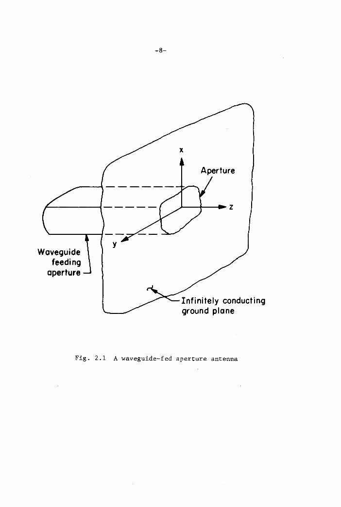
We consider an aperture in an infinitely conducting ground

plane at z = 0, fed by a cylindrical waveguide of arbitrary cross-

section located in the region z < 0, and radiating into a region

z > ° whose parameters may vary along the z-direction (Fig. 2.1).

Assuming the waveguide to be operating in its dominant mode,

only this mode will be incident on the aperture. However higher order

modes will be generated at the discontinuity and reflected back from

the aperture, along with the reflected dominant mode. The transverse

electric and magnetic fields at the aperture can be expressed as (19),

E (x,y) V e (x,y) +2: V e (x,y) (2.1)-0 0-0 n -n

n

H (x,y) = I h (x,y) +2:1 h (x,y) (2.2)-0 0 -0 n -n

n

Here V and I represent the total (incident plus reflected) amplitudeo 0

of the dominant mode, V and I represent the amplitudes of the re-n n

fleeted high order TE and TM modes. The transverse mode functions

-8-

Waveguidefeeding

aperture

Infinitely conductingground plane

Fig. 2.1 A waveguide-fed aperture antenna

e (x,y),"-1J

h (x,y)"-1J

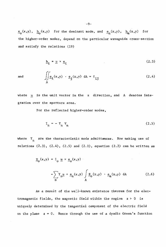
-9-

for the dominant mode, and e (x,y),-n

h (x,y)-n

for

the higher-order modes, depend on the particular waveguide cross-section

and satisfy the relations (19)

h. u x e. (2.3)-J. -J.

and JJ!:'i (x ,y) • e.(x,y) dA = o.. (2.4)-J J.J

A

where u is the unit vector in the z direction, and A denotes inte-

gration over the aperture area.

For the reflected higher-order modes,

In

y Vn n

(2.5)

where Yare the characteristic mode admittances. Now making use ofn

relations (2.3), (2.4), (2.5) and (2.1), equation (2.2) can be written as

1!o(x,y) = I u x e (x,y)o -0

- \'Y u x e (x,y) JE (x,y) • e (x,y) dAL n- -n "-1J -nn A

(2.6)

As a result of the we~l-known existence theorem for the e1ec-

tromagnetic fields, the magnetic field within the region z > 0 is

uniquely determined by the tangential component of the electric field

on the plane z = O. Hence through the use of a dyadic Green's function

-10-

g, the magnetic field in the region z > ° can be expressed as (2)

!!.(x,y,z) = f f. (x,x',y,y',z,o).~x ~(x',y') dA' (2.7)

A

The Green's function depends on the parameters of the region z > °and satisfies an appropriate differential equation with boundary condi-

tions. The integration in (2.7) is over the aperture area only, since

the tangential electric field vanishes over the conducting ground plane.

The continuity of the tangential magnetic field at the plane

z = ° results in the relation

u x H (x,y) = u x H (x,y,O)-0

(2.8)

Substituting (2.6) and (2.7) in (2.8) we obtain an integral equation for

the aperture electric field:

I e (x,y) = \' Y e (x,y) fE (x,y).e (x,y) dA0-0 L rrn -0 --n

n A(2.9)

- ~ u x g(x,x',y,y',O,O)

A'

xu· E (x' ,y') dA'-0

The admittance of the waveguide-fed aperture is defined as the

ratio of the total dominant mode magnetic to electric field amplitudes.

Y = I Ivo 0

(2.10)

-11-

A variational expression for Y can be obtained if equation

(2.9) is scalarly multiplied by E (x,y),-0

area A and then divided through by V2 =o

The result is

integrated over the aperture

2[f E (x,y) . e (x,y) dA] •A-o -0

[J~ (x,y) •

A

Y1

e (x,y)-0

(2.11)

-.if !o(x,y) • (~x G(x,x' ,y,y' ,0,0) x~)AA'

• E (x' y' ) dAdA}--0 '

If the exact aperture electric field were known, the admittance

Y could readily be found from (2.11). The exact field could only be

found by solving the integral equation (2.9), which, in general, is an

almost impossible task. Hence approximate methods must be devised, and

one such method consists in writing Y as a variational expression. The

expression (2.11) is stationary with respect to small variations oEo

of the aperture electric field Eo

about its exact value determined by

the integral equation (2.9). This means that substitution of an approx-

imate aperture electric field into (2.11) will still yield a good

estimate for Y. Furthermore, expression (2.11) is seen to be homo-

geneous in Eo

It is easy to verify that the variation of Y due to small

variations oE of E disappears. Making use of the symmetry propertyo 0

of the Green's function (2),

-12-

G.. (x,x' ,y,y' ,0,0) = G.. (x' ,x,y' ,y,O,O)1J J1

we obtain for the variation of Y,

(2.12)

e-0

e-0

(2.13)

The right-hand side of (2.13) may be rewritten as

. ~ dA - f (~ x .Q. x~) • ~A'

oE-0

dA

The expression in brackets under the integral sign vanishes because of

the integral equation (2.9). Hence

oY ° (2.14)

The variational expression (2.11) can be put in the more

convenient form

~E (x,y) x H (x,y) • u dA U~(x.y) . e (x,y) d~ 2-0 -0 -n

A LY AY U~(x,y)+ (2.15)

dAJ2

n n [J~(x.y) df. e (x,y) . e (x,y)-0 -0

A A

-13-

provided it is understood that the function to be varied is E (x,y),-0

and that H (x,y) = H(x,y,O) is related to E (x,y) through equation-0 -0

(2.7). This requires finding an appropriate Green's function, which, in

practice, may be quite difficult. Instead it is easier to find a

relation between the Fourier components of the electric and magnetic

fields, as will be shown in the next chapter.

The most simple and logical assumption is that the aperture

electric field has the form of the dominant mode. Then

E (x,y)-0

V e (x,y)o -0

(2.16)

and the second term in (2.15) involving the summation vanishes because

of (2.4). Thus for dominant mode aperture electric field approximation

the admittance becomes

y = -lz-j E (x,y) x H (x,y) • u dAV -0 -0

o A

(2.17)

where it is understood that

relation like (2.7).

H-0

is linearly related to E-0

through a

Comparisons of theoretical and experimental results have shown

that the dominant mode aperture electric field approximation is adequate

in most instances (11, 14, 20). However, for a more exact treatment,

the aperture electric field could be assumed as a superposition of the

dominant mode and some higher order modes. For simplicity let us

consider only one higher order mode, with mode function e., which would-~

be the next most highly excited mode, as indicated by the geometry of the

-14-

problem. The generalization to more than one, but a finite number of

higher order modes will be evident. Accordingly, the aperture electric

field could be written as

= E (x,y) + a. E .(x,y)c::.o 0 J. -0 J.

The resulting aperture magnetic field would be

H (x,y) = H (x,y) + a. H . (x,y)-0 -00 J. -OJ.

(2.18)

(2.19)

with .!!aO,i(x,y) =JSb (x,x',y,y') . u x ~o,i(x',y') dx'dy'

A

Making use of the symmetry of the Green's function, the

aperture admittance becomes in this case,

Y = _1{IE x HV 2 -00 -00

o A

udA+ 2a. fiJ. -00

A

x .!!ai • u dA

+ a.2JE .

J. -OJ.

A

x H .• U-OJ.

Y.J.

2= y + 2a. y . + a. (y .. + Y.)

00 J. OJ. J. J.J. J.(2.20)

-15-

where

x Hon udA (2.21)

y .. + Y.~~ ~

Since Y is stationary,

that dY/da. = O. Hence,~

Yoia. - - ----~

a. is determined from the condition~

(2.22)

Substituting (2.22) into (2.20) we finally obtain

Y = Yoo -y .. + Y.~~ ~

(2.23)

The first term in (2.23) is the result of assuming an aperture

electric field of the form of the dominant mode, and is the same as

(2.17). It is also evident from equation (2.23) that when higher order

modes are included a mutual coupling exists between the modes. Further-

more, the terms in equation (2.23), Yoo ' Yoi ' Yii , are of the form of

(2.17), which suggests that once a method is known for finding the

admittance assuming an aperture electri.c field of the form of the

dominant mode, extension to a more general case is straightforward.

Hence, in the future, only equation (2.17) will be considered.

-16-

3. APERTURE ANTENNA CHARACTERISTICS

This chapter will deal with the derivation of some important

relations for the calculation of the aperture admittance and the

radiation pattern of the radiating structures that are being considered.

The results will apply to any aperture shape and to most media of

physical interest where the antenna is radiating. The method used is

new, yet quite simple, in that it bypasses the usual boundary-value

approach.

A. Plane Wave Synthesis of Aperture Distributions

It is well known that an arbitrary time-harmonic field can

be constructed by a superposition of plane waves, all of the same

frequency, each with its appropriate amplitude, and traveling in all

possible directions, real as well as complex (21).

The region z < 0 of Fig. 2.1 in which the waveguide is

located will now be considered as a semi-infinite region of free space

where plane waves propagating in every possible direction are incident

on and reflected from the half-space z > 0, in such a way that on the

plane z = 0 a specified electric field configuration is obtained.

This field will be the assumed aperture electric field over the aperture

area, and will vanish everywhere else. Looking at the problem in this

way, the evaluation of the aperture admittance and the radiation pattern

will be greatly simplified, particularly if the structure is radiating

into an inhomogeneous medium. It will be shown that the double Fourier

transform E (u,v)-0

of the aperture electric field E (x,y) is simply-0

-17-

related to the amplitudes of the plane waves in the region z < O. The

calculation of the reflection and transmission coefficients for each

plane wave will enable the computation of the aperture admittance and

the radiation pattern.

A plane electromagnetic wave of frequency w, traveling in

free space can be represented by,

ikn·rE e

(3.1)

where k = ~,o 0

is a unit vector in

nW, E is the complex wave amplitude,o

the propagation direction, n' E = 0, and an

n

-iwte time dependence is understood.

We now suppose that such a plane wave traveling in the region

z < 0 is incident on the boundary at z = 0, and use the subscript i

to denote the incident fields and the unit vector in the propagation

direction of the incident wave.

The plane containing the vector in the direction of propagation

(n.) and the normal to the boundary is called the plane of incidence.-).

It is well known that any plane electromagnetic wave can be resolved into

two components, one with the electric vector polarized perpendicular to

the plane of incidence, and another for which the electric vector lies

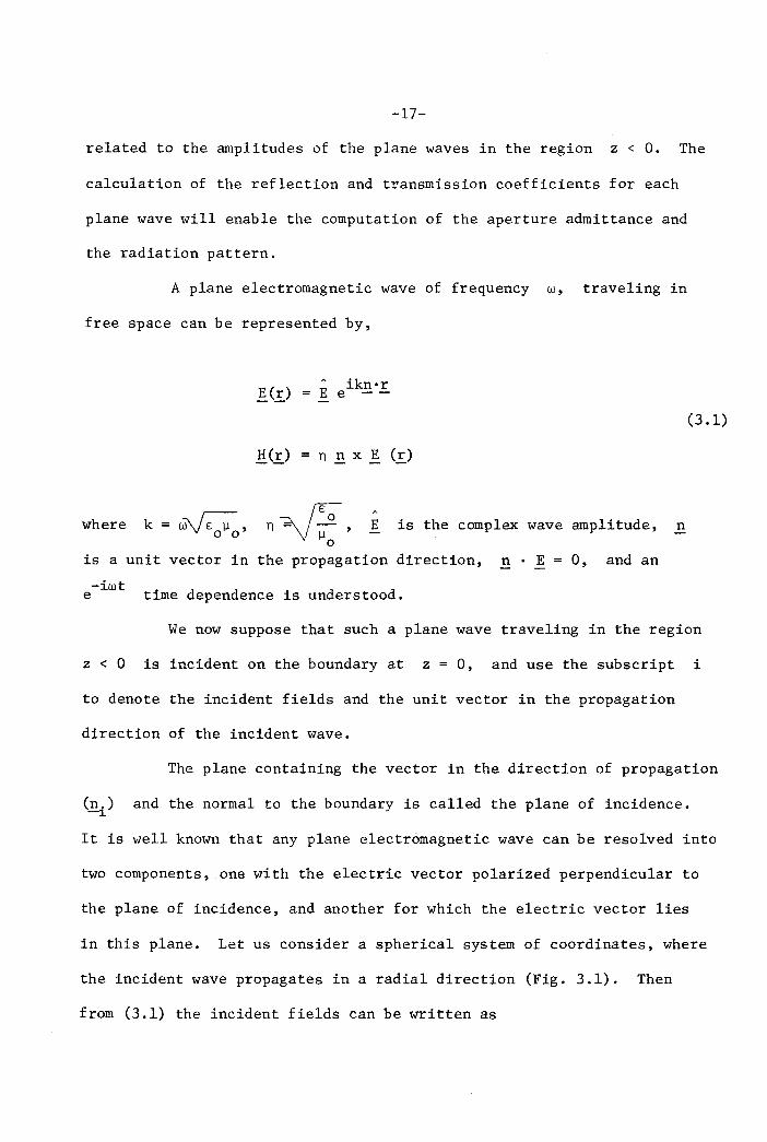
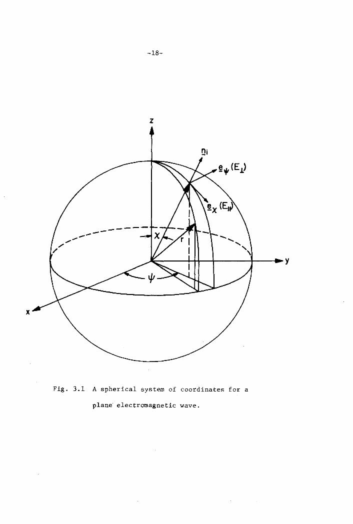
in this plane. Let us consider a spherical system of coordinates, where

the incident wave propagates in a radial direction (Fig. 3.1). Then

from (3.1) the incident fields can be written as

x

-18-

z

n·_I

~---4-+I---+-----t--~Y

Fig. 3.1 A spherical system of coordinates for a

plane electromagnetic wave.

-19-

E. (r) = (E ~\jJ + E e ) ikn. 're -1. --1. - 1. 11)(

(3.2)

!!i (.E.) neE E e) ikn. 're e -1. -111 1.)(

where ~i' ~ and ~ are unit vectors in the radial, polar and

azimuthal direction (Fig. 3.1). Clearly, the azimuthal component of

the incident electric field is perpendicular to the plane of incidence,

hence it is denoted as E1.' while the polar component lies in this

plane and is denoted as Ell' Often the perpendicular polarized component

is referred to as transverse electric (TE), while the parallel po1ar-

ized component is called transverse magnetic (TM).

The phase of the incident plane wave can be written as

n .• r = ux + vy + wz---J..

(3.3)

where the direction cosines u, v, w of the vector n.-1.

are expressed

in terms of the polar and azimuthal angles X and \jJ as

u = sin X cos \jJ

v sin X sin \jJ (3.4)

w cos X

The direction cosines obviously satisfy the relation222

u + v + w = 1.

Considering the geometry of the problem it will be more con-

venient to express the fields (3.2) in a circular cylindrical coordinate

-20-

system with z as the longitudinal axis. Accordingly we have

E. (r) (E.l.eljJ + Ell cos X e E sin X e )ik(ux+vy+wz)e

-1 - -p 1\ -z

0.5)

H. (r) n(EII~ E.l. cos X e + E.l. sin X e )ik(ux+vy+wz)e

-1 -p -z

where e is a unit vector in the radial direction on the plane trans­-p

verse to the z-axis, and we will let

The unit vector in the z direction is now denoted as e.-z

Part of this incident wave will be reflected back from the

boundary at z = 0, while part will be transmitted into the region

0.6)

z > O. The fields of the reflected wave have also the form of (3.1),

but now the subscript r will be used to denote them as well as the

unit vector in the propagation direction of the reflected wave. It

follows from the laws of reflection at a plane boundary that this unit

vector can be written as

n = sin X e - cos X e-r -p -z

0.7)

u e + v e-x --y

w e-z

and hence the phase of the reflected wave is

n . r = ux + vy - wz-r 0.8)

-21-

Remembering that the perpendicular and parallel polarized

components of the wave have different reflection coefficients, and de-

noting them by f.L and respectively, the reflected fields E (r)-r -

and H (r) can be written from (3.1) and (3.7) as-r -

E (r)-r -

H (r)-r -

(E f !:'ljJ + E\lf\l cos X e + E f sin ) ik(ux+vy-wz)X e e

.L .L -p II II -z

(3.9)

n(-E f eljJ + E f cos X e + E.Lf.L sin ) ik(ux+vy-wz)X e e

1111- .L .L -p -z

The sum of (3.5) and (3.9) represents the total fields in

the region z < 0, arising from a single plane wave, propagating in

a given direction, which is incident on and reflected from the boundary

at z = O. The propagation direction of the incident wave changes as

one varies the direction cosines u and v (or equivalently, the

angles X and ljJ). Associating with the waves propagating in the cone

u + du, v + dv two complex amplitudes, one for perpendicular polar-

" 2ization E.L(u,v)k dudv, and another for parallel polarization

" 2E11(u,v)k dudv, and integrating (3.5) and <3.9) over all possible

directions of propagation, we can represent the most general fields in

the semi-infinite region z < 0, bounded by the surface at z = 0 (21).

Thus,

00

(3.l0a)

", /1 2 (e ikwz f -ikwz) ) ik(ux + VY)k2d dE IV - w - lie !:'z e u v

-22-

00

(3.l0b)

+ E'JI 2(e ikwz + r e-ikwZ)e~eik(UX + VY)k2dudv- w

.L .L -z

where =-Vl2 2

(3.11)w - u - v

and e-p

are all functions of u and v.

The fact that the limits of integration are from _00 to +00 implies

that complex angles for the propagation direction are also included.

This is necessary in order to represent arbitrary fields in the region

z < O.

The amplitude functions E.L(u,v) and Ell (u,v) can now be

expressed in terms of the prescribed electric or magnetic field on the

plane z = O. If the electric field distribution is specified on the

plane z = 0, then, the continuity of the tangential electric field

requires that this must equal the transverse electric field at z = a

obtained from (3.lOa). Thus

00

.J;,(x,y) t {EL(u,v)(l + r L (u,v))-'4 + Ell (u,v)w(l + rll(u,v)~

(3.12)

The expression within the brackets under the integral sign in

Eq. (3.12) can be recognized as the two-dimensional Fourier transform of

-23-

the specified electric field distribution E (x,y).-0

Then

E (u,v)-0

00

[~'IT]2JJ ~(x,y) e-ik(ux + VY)dxdy

-00

(3.13)

EJ.(u,v) (1 + fJ.(U'V»~ljJ + Ell (u,v)w(l+ fll(u,v»~

It immediately follows from (3.13) that

Em/! (u, v)

1 + r (u,v)J.

(3.l4a)

andA

Ell (u, v)E (u,v).e E (u,v)

_-o-=- ::P.L-_ = _-=oJ;.p~ _

w(l + f ll (u,v» w(l + fll

(u,v)(3.l4b)

In terms of the specified electric field E (x,y) on the plane-0

z = 0, the fields in the region z < ° are now given by Eqs. (3.10),

(3.13) and (3.14). Of course, the reflection coefficients f (u,v)J. and

fll(U,V) for plane waves traveling in the (u,v) direction, and incident

on the boundary at z = 0, must be known. These plane wave reflection

coefficients depend also on the constitutive parameters of the medium

in the region z > 0, which does not have to be homogeneous in the z

direction.

Finally, the magnetic field on the plane z = 0, H (x,y),-0

and its Fourier transform,

00

H (u,v)-0

are given by,

n l{ ~I (u,v)(l - "II (u,v))~ - E" (u,v)w(l r (u,v»eJJ. -,

(3.15)

00

!ic(u,v) =[~;J2 jJ!ic(X,y)_00

-24-

-ik(ux + vy)e dxdy

(3.16)

n ( Ell (u, v) (1 - r ll (u, v) )~ljJ - El. (u, v)w(l

It can readily be seen that the magnetic field on the plane

z = 0 is a function of the specified electric field on that plane.

B. Aperture Admittance

The results of the preceding paragraphs will now be used to

obtain a general expression for the admittance of flush-mounted aperture

antennas. For dominant mode aperture electric field approximation the

admittance can be rewritten from (2.17) as

y ~ (( E* (x,y) x H (x,y) .V JJ -0 -0

o A

e-z dxdy (3.17)

The asterisk denotes complex conjugates. Obviously this expression is

the same as (2.17) since a real aperture field distribution is always

assumed. Applying Parseval's theorem to (3.17) the admittance becomes

y

00

[~:Jif i;<u,v) x_00

H (u,v)-0

2• e k dudv-z (3.18)

Using (3.13) and (3.16), and then (3.14)

-25-

~*

E x H-0 -0

1 - f.L

1 + f.L

(3.19)

The ratio of the tangential components of the magnetic and

electric fields of the plane waves at the boundary surface z = 0 may

be called the input admittance of the region z > 0, and is given, for

each direction of polarization, in terms of the reflection coefficients

by (22)

Y. (u,v)1. 0 .L

(3.20a)

1 + fll(u,v)and

1 - fll(u,v)Y. (u, v) = (n/w)

1.0 I!(3.20b)

Relations (3.18), (3.19) and (3.20) can now be used to obtain

a general expression for the admittance of a flush-mounted, waveguide-fed

aperture antenna with the dominant mode aperture electric field approxi-

mation. The result is

Y~ 2

Y. (u,v) + IE (u,v)1 Y. (u,v)l.n.L op 1.n il

dUdV) 0.210)

or equivalently,

y

-26-

A 2 }Y. (p) + IEOp(p,lj!) I Y. (p) pdpdlj!lnJ. lnll

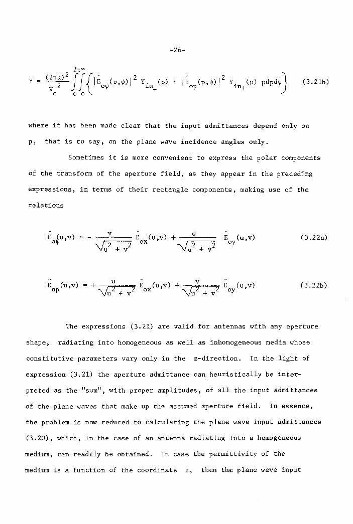
(3.2lb)

where it has been made clear that the input admittances depend only on

p, that is to say, on the plane wave incidence angles only.

Sometimes it is more convenient to express the polar components

of the transform of the aperture field, as they appear in the preceding

expressions, in terms of their rectangle components, making use of the

relations

v

-Vu2 + 2v

E (u,v) + __u _

ox '\fu2 + v2E (u,v)oy (3.22a)

E (u,v)op = + 'J u 2 E (u,v) + ¥ ~ 2 E (u,v)u 2 + v ox u + v oy

(3.22b)

The expressions (3.21) are valid for antennas with any aperture

shape, radiating into homogeneous as well as inhomogeneous media whose

constitutive parameters vary only in the z-direction. In the light of

expression (3.21) the aperture admittance can heuristically be inter-

preted as the "sum", with proper amplitudes, of all the input admittances

of the plane waves that make up the assumed aperture field. In essence,

the problem is now reduced to calculating the plane wave input admittances

(3.20), which, in the case of an antenna radiating into a homogeneous

medium, can readily be obtained. In case the permittivity of the

medium is a function of the coordinate z, then the plane wave input

-27-

admittances will be obtained, in the next chapter, by a special method.

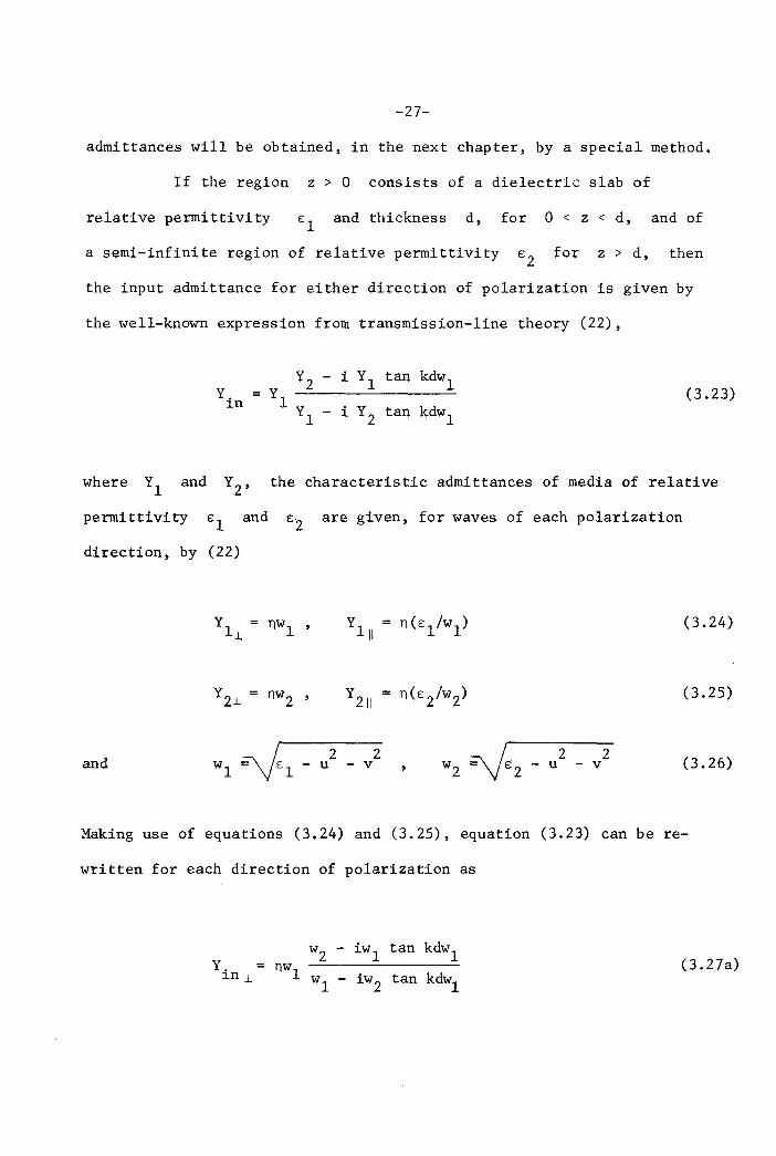
If the region z > a consists of a dielectric slab of

relative permittivity and thickness d, for a < z < d, and of

a semi-infinite region of relative permittivity £2 for z > d, then

the input admittance for either direction of polarization is given by

the well-known expression from transmission-line theory (22),

Y.l.n

(3.23)

where Yl

and Y2 , the characteristic admittances of media of relative

permi ttivi ty and £2 are given, for waves of each polarization

direction, by (22)

nWl ' (3.24)

(3.25)

and2

- u2

- v2

- u2

- v (3.26)

Making use of equations (3.24) and (3.25), equation (3.23) can be re-

written for each direction of polarization as

Y.l.n .L

tan kdwl

tan kdwl

(3.27a)

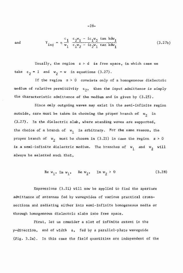
and Y.l.nll

-Z8-

EZwl - iElwZ tan kdw iEl w2 - iEZwl tan kdw

1(3.27b)

Usually, the region z > d is free space, in which case we

take E = IZ

and w in equations (3.27).

If the region z > 0 consists only of a homogeneous dielectric

medium of relative permittivity EZ' then the input admittance is simply

the characteristic admittance of the medium and is given by (3.25).

Since only outgoing waves may exist in the semi-infinite region

outside, care must be taken in choosing the proper branch of w2 in

(3.27). In the dielectric slab, where standing waves are supported,

the choice of a branch of is arbitrary. For the same reason, the

proper branch of w2 must be chosen in (3.25) in case the region z > 0

is a semi-infinite dielectric medium.

always be selected such that,

The branches of and will

Re WI' 1m wI' Re w2 ' (3.28)

Expressions (3.21) will now be applied to find the aperture

admittance of antennas fed by waveguides of various practical cross-

sections and radiating either into semi-infinite homogeneous media or

through homogeneous dielectric slabs into free space.

First, let us consider a slot of infinite extent in the

y-direction, and of width a, fed by a parallel-plate waveguide

(Fig. 3.2a). In this case the field quantities are independent of the

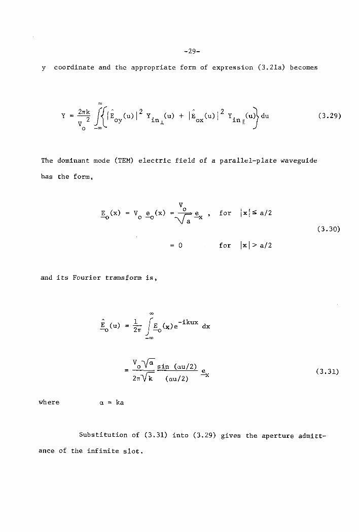
-29-

y coordinate and the appropriate form of expression (3.2la) becomes

00

y = 2nk f{IE (u)[2V 2 oy

o _00

A 2 Jy. (u) + IE (u)l y. (u) du1.n J. ox 1.n \I

(3.29)

The dominant mode (TEM) electric field of a parallel-plate waveguide

has the form,

VE (x) V e (x) 0 for Ixl:::;; a/2=~e

-0 o -0 -v;.-x

(3.30)

0 for lxl>a/2

and its Fourier transform is,

00

E (u) = 1- fE ( )e-ikux dx-0 2n -0 x

_00

where a = ka

V0 -va sin (au/2)

2n-{k (au/2)e-x (3.31)

Substitution of (3.31) into (3.29) gives the aperture admitt-

ance of the infinite slot.

-30-

00

y =%J sin2

(au/2)y. (u) du (3.32)

2(au/2) lnll0

Next, we consider a rectangular waveguide with smaller cross-

sectional dimension a and larger dimension b (Fig. 3.2b). The

dominant mode (TEla) electric field can then be written as

E (x,y)-0

V e (x,y)o -0

V~ cos p- ~x' for Ixl s;; a/2, Iyl s;; b/2

(3.33)

= a otherwise

The Fourier transform of this aperture field becomes

E (u,v)-0

~ff .J;,(x,y) e-ik(ux + vy) dx dy

_00

V~o as= 27Tk 8"

sin (au/2)(au/2)

cos (Sv/2)e

(7T/2)2 _ (Sv/2)2-x(3.34 )

where a = ka , S = kb (3.35)

Substitution of (3.34) into expressions (3.21) give the

admittance of rectangular waveguide-fed apertures

-31-

I I I I Z I I I I I I l~ I I t I I I 2 Z I Z~

-CD to CD I4- ~y --. a

II Z II Z lIlIllllllllllll Z~a b

1

14---- 2b--~

c

14---2a--~

d

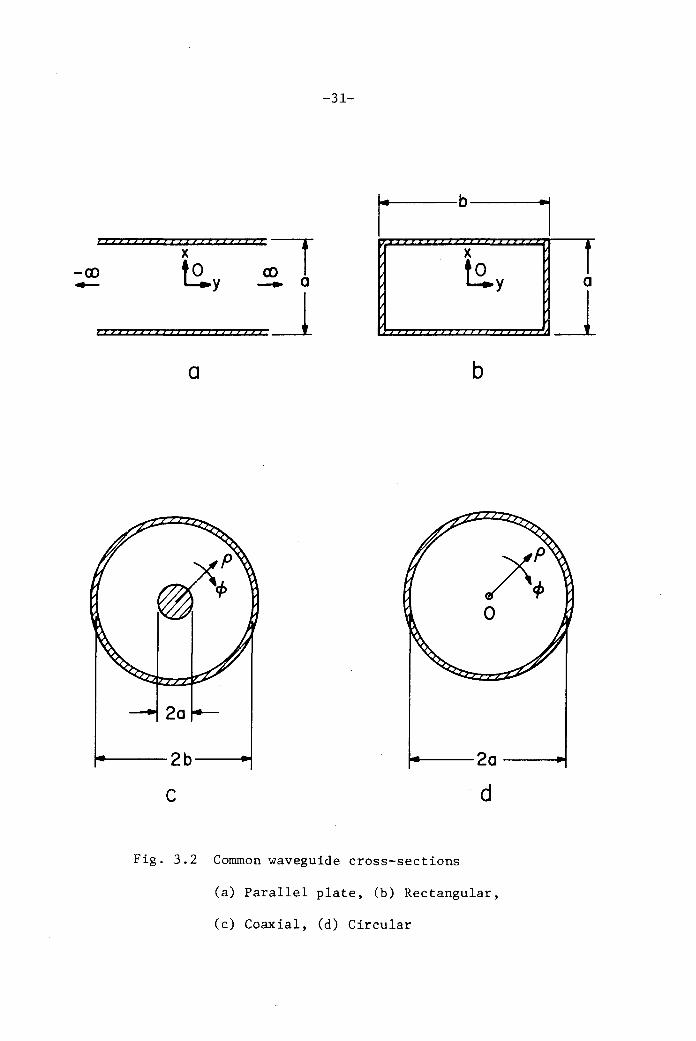
Fig. 3.2 Common waveguide cross-sections

(a) Parallel plate, (b) Rectangular,

(c) Coaxial, (d) Circular

-32-

y = "~~~[S~~~/~i2)_00_00

00 00

or equivalently,

CO~(SV/2) ZJZ{y (U,V);Z 2 + Y. (u,v) UZ

2Z~dUdV

(TI/Z) - (Sv/Z) in.l.. u +v l.nll u +v')

(3.36a)

2TI 00

Y = as l~Sin ( ¥cosl/J) cos (¥ sin llJ) ~t2 .8 Z l.n (p)

o (¥ cos l/J) (; )2 (¥ sin l/J) .1.

cos 2l/J+Y. (p)sin2~pdpdl/Jl.nll )

0.36b)

For a coaxial waveguide of inner conductor radius a, and outer

conductor radius b (Fig. 3.Zc), the dominant mode (TEM) electric field

at the aperture is given by

~(p,<j» V e (p) =o -1)

Vo 1

-V Z7r -fn(b/a) pe ,-p

for a < p < b

= 0

The transform of this field is readily found to be

otherwise (3.37)

27r 00

Jf ~(p,<j»o 0

e-ikpp cos (<j>-l/J) pdp d<j>

Vi 0

= 2TI IiZTI -fn(S/a)e-p

0.38)

-33-

Hence, the admittance of an annular aperture fed by a coaxial

waveguide becomes from (3.2Ib) and (3.38),

Y = in (3.39)

Finally we consider a circular waveguide of radius a (Fig. 3.2d)

whose dominant mode (TEI1)electric field is given by

V e (p, <1»o -0

< a

(3.40)

= 0 for p > a

where

and x' is the first root of11

J I (x) = 0I

The transform of this field must then be calculated and the

final result turns out to be

2'IT 00

i,(p,oP) = [~;T11 ~(p,.)e-ikPPCOS(.-oP)PdP doP

o 0

-34-

(3.41)

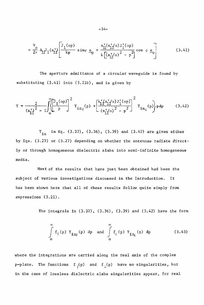
The aperture admittance of a circular waveguide is found by

substituting (3.41) into (3.2lb), and is given by

2 f""@l(ap)j 2 ~xJ.lxiia)Ji (ap)j 2 jy = ---=2-- Y. (p) + 2 2 Y. (p) pdp(xIi. - loP l.nll (xl{a) _ p l.nJ.

(3.42)

Y. in Eq. (3.32), (3.36), (3.39) and (3.42) are given eitherl.n

by Eqs. (3.25) or (3.27) depending on whether the antennas radiate direct-

ly or through homogeneous dielectric slabs into semi-infinite homogeneous

media.

Most of the results that have just been obtained had been the

subject of various investigations discussed in the Introduction. It

has been shown here that all of these results follow quite simply from

expressions (3.21).

The integrals in (3.32), (3.36), (3.39) and (3.42) have the form

""

f fll (p) Y. (p) dp1.nil

o

and""JfJ. (p)

o

(3.43)

where the integrations are carried along the real axis of the complex

p-plane. The functions f \I(p) and f J.(p) have no singularities, but

in the case of lossless dielectric slabs singularities appear, for real

Hence care must be taken in calculating

-35-

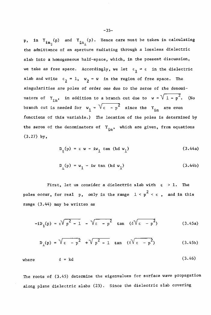
p, in Y. (p) and Y. (p).1n\l 1n.L

the admittance of an aperture radiating through a lossless dielectric

slab into a homogeneous half-space, which, in the present discussion,

we take as free space. Accordingly, we let ~l = ~ in the dielectric

slab and write ~2 = 1, w2 = w in the region of free space. The

singularities are poles of order one due to the zeros of the denomi­

nators of Y. , in addition to a branch cut due to w =-y 1- p2. (No1n

branch cut is needed for wl

= -y~ 2- p since the Y.

1nare even

functions of this variable.) The location of the poles is determined by

the zeros of the denominators of Y. , which are given, from equations1n

(3.27) by,

(3.44a)

(3.44b)

First, let us consider a dielectric slab with ~ > 1. The

poles occur, for real p, only in the range2

I < p < e: and in this

range (3.44) may be written as

e:-Y p2 - 1 - -V e:

2- p tan (3.45a)

2- p tan

2- p ) (3.45b)

where o = kd (3.46)

The roots of (3.45) determine the eigenvalues for surface wave propagation

along plane dielectric slabs (23). Since the dielectric slab covering

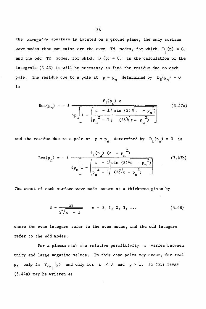
-36-

the waveguide aperture is located on a ground plane, the only surface

wave modes that can exist are the even TM modes, for which D (p) = 0,II

and the odd TE modes, for which D (p) = 0.J.. In the calculation of the

integrals (3.43) it will be necessary to find the residue due to each

pole. The residue due to a pole at p = Pn determined by DII(Pn) = °is

Res(p )n

(3.47a)

and the residue due to a pole at p = Pn determined by DJ..(Pn) = ° is

Res(p ) =n (3.47b)

The onset of each surface wave mode occurs at a thickness given by

nTl"o = -;::=====2\1 E - 1

n = 0, 1, 2, 3, ... (3.48)

where the even integers refer to the even modes, and the odd integers

refer to the odd modes.

For a plasma slab the relative permittivity E varies between

unity and large negative values. In this case poles may occur, for real

P, only in Yin (p) and only for E < ° and p > 1. In this rangeII

(3.44a) may be written as

iD 11 (p)

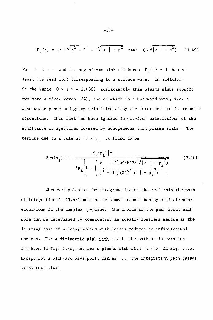
-37-

(3.49)

For E: < - 1 and for any plasma slab thickness D11 (p) = 0 has at

least one real root corresponding to a surface wave. In addition,

in the range 0 > E: > - 1.0363 sufficiently thin plasma slabs support

two more surface waves (24), one of which is a backward wave, i.e. a

wave whose phase and group velocities along the interface are in opposite

directions. This fact has been ignored in previous calculations of the

admittance of apertures covered by homogeneous thin plasma slabs. The

residue due to a pole at p = Pi is found to be

Res (p.)1

(3.50)

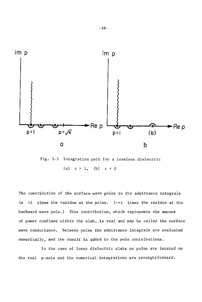
Whenever poles of the integrand lie on the real axis the path

of integration in (3.43) must be deformed around them by semi-circular

excursions in the complex p-plane. The choice of the path about each

pole can be determined by considering an ideally loss less medium as the

limiting case of a lossy medium with losses reduced to infinitesimal

amounts. For a dielectric slab with E: > 1 the path of integration

is shown in Fig. 3.3a, and for a plasma slab with E: < 0 in Fig. 3.3b.

Except for a backward wave pole, marked b, the integration path passes

below the poles.

1m p

-38-

1m p

Re p Re pp= I p=j€ p= I ( b)

a b

Fig. 3.3 Integration path for a loss less dielectric

(a) £ > 1. (b) E: < 0

The contribution of the surface wave poles to the admittance integrals

is ni times the residue at the poles. (-ni times the residue at the

backward wave pole.) This contributj.on. which represents the amount

of power confined within the slab. is real and may be called the surface

wave conductance. Between poles the admittance integrals are evaluated

numerically. and the result is added to the pole contributions.

In the case of lossy dielectric slabs no poles are located on

the real p-axis and the numerical integrations are straightforward.

-39-

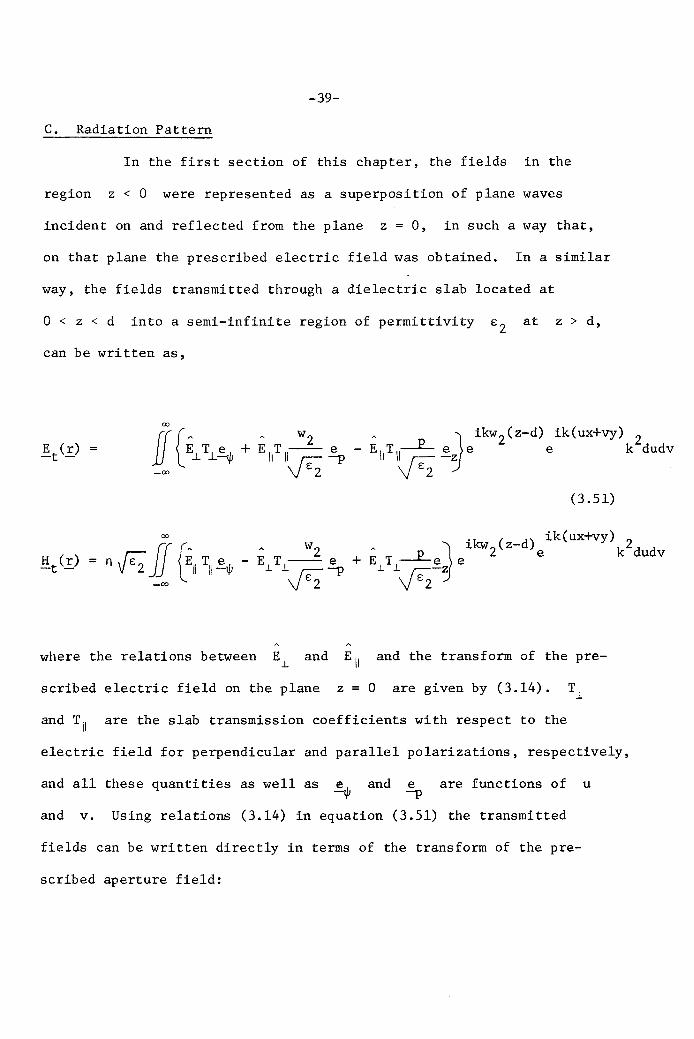
c. Radiation Pattern

In the first section of this chapter, the fields in the

region z < 0 were represented as a superposition of plane waves

incident on and reflected from the plane z = 0, in such a way that,

on that plane the prescribed electric field was obtained. In a similar

way, the fields transmitted through a dielectric slab located at

o < z < d into a semi-infinite region of permittivity £2 at z > d,

can be written as,

00

, ~ ikw2 (z-d) ik(.-vy) 2If (EJ-T.L~~A w2

E (r) + EIITII-- e EIITI~ ~z e e k dudv-t -

_00

vs;.-p £2

(3.51)

00 ikw (z-d) ik(ux+vy) 2

H (r) n v;:; ff (Ell Til ~~A W2

E"\ft~~~e2 e k dudv

= E.lT.l-- e +-t - \f£;-P_00

where the relations between E.l and E II and the transform of the pre-

scribed electric field on the plane z = 0 are given by (3.14). T.l

and Til are the slab transmission coefficients with respect to the

electric field for perpendicular and parallel polarizations, respectively,

and all these quantities as well as e and e are functions of u-~ -p

and v. Using relations (3.14) in equation (3.51) the transmitted

fields can be written directly in terms of the transform of the pre-

scribed aperture field:

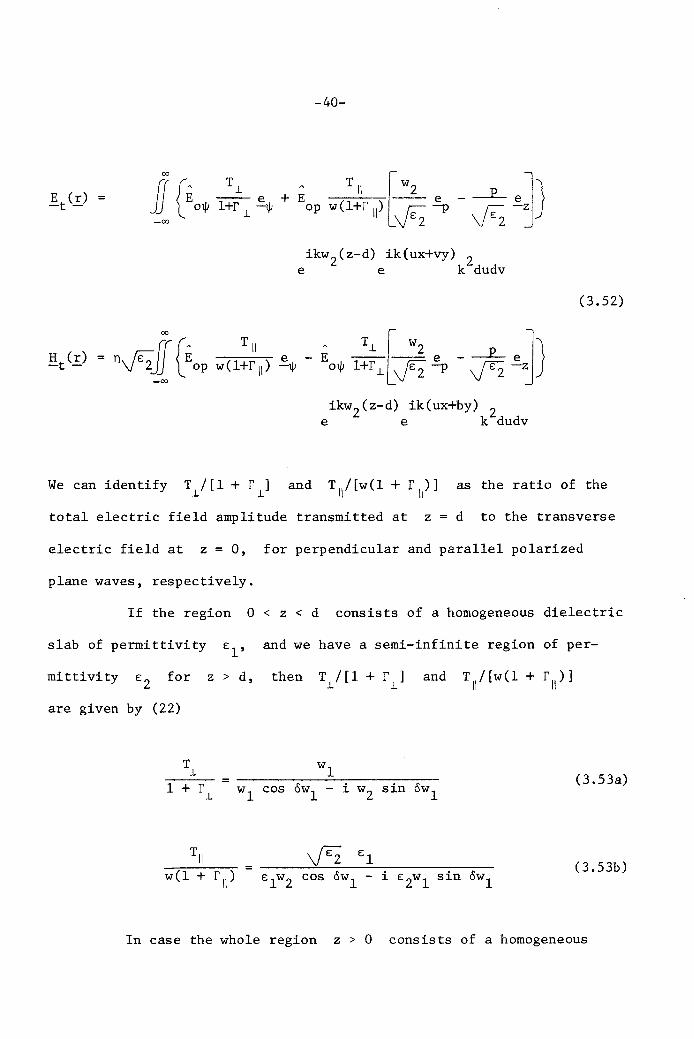
-40-

E (r)-t -

ikw2

(z-d) ik(ux+vy) 2e e k dudv

(3.52)

00

"J"zff lEop -w-'-(l-:-~II-:-I) ~ -_00

ikw2 (z-d) ik(ux+by) 2e e k dudv

We can identHy T /[1 + r ].1 .1

and T \I / [w(1 + r \I) ] as the ratio of the

total electric field amplitude transmitted at z = d to the transverse

electric field at z = 0, for perpendicular and parallel polarized

plane waves, respectively.

If the region 0 < z < d consists of a homogeneous dielectric

slab of permittivity £1' and we have a semi-infinite region of per-

mittivity £2 for z > d,

are given by (22)

then T /[1 + r ].1 .1

(3.53a)

(3.53b)

In case the whole region z > 0 consists of a homogeneous

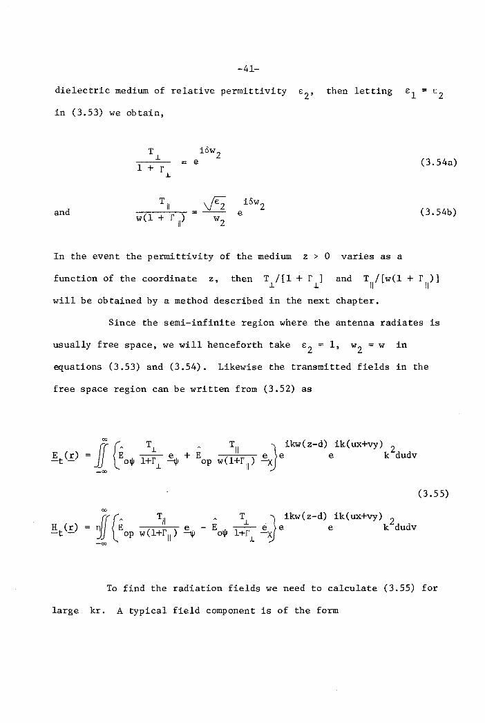
-41-

dielectric medium of relative permittivity E2

, then letting E l = E 2

in (3.53) we obtain,

T iow2.L= e

1 + r.1.

andTil VE2 iOw2

w(l + r II)=-- ewz

In the event the permittivity of the medium z > 0 varies as a

(3.54a)

(3.54b)

function of the coordinate z, then T /[1 + r ].L .L

will be obtained by a method described in the next chapter.

Since the semi-infinite region where the antenna radiates is

usually free space, we will henceforth take E 2 = 1, w2 = w in

equations (3.53) and (3.54). Likewise the transmitted fields in the

free space region can be written from (3.52) as

E (r)-t -

Til Jikw(z-d) ik(ux+vy) 2+ E e e e k dudv

op w(l+rll

) -X

H (r)-t -

(3.55)

00

~ ~EAOp _-,--T'_I-:-- T Jikw(z-d) ik(ux+vy) Z

~" - EO'"

l;-.Lr ~X e e k dudvw(l+r ll ) 'I' 'I' .L-00

To find the radiation fields we need to calculate (3.55) for

large kr. A typical field component is of the form

00

g (.E.) = ff g(u , v)

_00

-42-

ikrf(u,v) 2e k dudv (3.56)

where, using spherical coordinates for the space variables, f(u,v)

becomes

f(u,v) ,.. cos eJl -u2

- v2 + sin e (cos ep u + sin ep v) (3.57)

The double integral (3.56) can be readily evaluated for large kr by

applying twice the method of stationary phase. The point where

f (u,v) = f (u,v) = 0, so that the phase is "stationary", is given by,u v

u = sin e cos epo

v sin e sin epo

(3.58)

and the result of the integration of (3.55) to first order in l/kr

turns out to be (25,26)

(3.59)

The stationary phase integration of (3.56) is easy to inter-

pret. We see that out of all the plane waves propagating in directions

determined by u and v, and making up the fields at the observation

point in the region z > d, only the wave that travels in a radial

direction toward that point contributes significantly to the radiation

field.

In the case of the waveguide aperture radiating through a

-43-

loss less dielectric slab, singularities may appear on the path of

integration, in the integrand of (3.56). Then, an evaluation of the

integral by the method of steepest descent (15,27) reveals that these

singularities, which correspond to surface waves, contribute to the

radiation field only for 8 = n/2, and that for 8 # n/2 the result

of the stationary phase analysis is still valid.

The far-zone fields follow from (3.55) and (3.59). Hence-

forth ~(8,~) will be written for g(u = sin 8 cos ¢, v = sin 8 sin ¢)o 0

to clearly denote the angular dependence of the far-zone fields. Thus

we have

E¢ (!)

(3.60)

T I\(8) -iocos8 eikr- 2in E (8,¢) e k cos 8

op w(8)(1+r 11 (8» r

(3.61)

For easy reference, the expressions for T/[1 + r J.] and TII/[w(l + r ll )]

can be written down as a function of 8. From (3.53) we have, letting

=l+r J.(e) -YE-sin

28

IfE - . 28S1n

(3.62a)

-44-

and

£

w(8) (l+f 11(8»(3.62b)

The radiation pattern~ which is proportional to the angular

dependent part of the far-zone Poynting's vector~ can be written as

E (8 ~¢)op

2 T 11(8) }w(8) (l+f 11(8» (3.63)

The far-zone fields and the radiation pattern of waveguide-

fed apertures radiating through a dielectric slab into free space are

given by (3.60)~ (3.61) and (3.63) in connection with (3.62). If the

apertures were radiating directly into free space~ i.e. if no dielectric

slab were present~ then the far-zone fields and the radiation pattern

would still be given by (3.60)~ (3.61) and (3.63)~ but with T/(1+f)=ei6w

as is readily evident from (3.54). Thus we see that the dielectric slab

has the effect of multiplying the components of the far-zone fields with

no dielectric slab present by the factors T~/(l + f~)

(given by (3.62) in case of a homogeneous slab) and

or Til / (1 + f ll )

-iOwe which depend

on e and the parameters of the dielectric medium~ provided that the

same aperture field distribution is assumed with or without the dielectric

slab.

To find the far-zone fields and the radiation pattern asso-

ciated with particular configurations the appropriate aperture field

transfonns must be evaluated and substituted in (3.60) and (3.63).

By way of example~ we will find the radiation pattern of a circular

aperture fed by a circular waveguide. The transform of the aperture

-45-

field is given by (3.41), and hence, apart from ignorable constants,

we have

X' (x'/a) J' (asin8)11 11 1

cos </>

(3.64)

E (8,</»op

Jl

(asin8)

k sin 8 sin </>

The radiation patterns for each of the two principal planes, the

xz-plane (</> = 0, 8 variable) and the yz-plane (</> = n/2, 8 variable)

are given respectively by

k2 A 2 TJ.(8) /2 2F(8,0) IEO1/! (8 ,0) I 1 + fJ.(8)cos 8

and (3.65)

k2

1E (8,n/2) 12 I Til (8) 2

F(8,n/2) =1 + f ll (8)op

where

where

EO

1/! (8,0)

T/(l + r)

and E (8,n/2) can be obtained from (3.64), andop

i6wequals e if the aperture radiates directly into

free space, and is given by equations (3.62) if it radiates through a

homogeneous dielectric slab into free space. It can further be noted

that F(8,O) and F(8,n/2) are proportional to the angular dependent

parts of IE</>(r,8,O)12

and !E8 (r,8,n/2) 12

respectively.

-46-

4. REFLECTION AND TRANSMISSION PROPERTIES OF

INHOMOGENEOUS DIELECTRIC SLABS

When a waveguide-fed aperture antenna is covered by an in­

homogeneous dielectric slab whose permittivity varies in a direction

perpendicular to the slab faces (the z-direction), then the expressions

developed in the previous chapter are adequate to calculate the aperture

admittance of the antenna as well as the radiation pattern, provided the

reflection and transmission coefficients of the inhomogeneous dielectric

slab are known. Accordingly, the present chapter will be devoted to the

calculation of these coefficients, and related quantities, for inhomo­

geneous dielectric slabs.

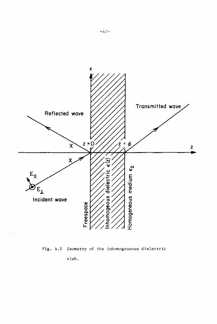
If the properties of the dielectric slab vary only in the

direction normal to its plane faces, then the reflection and transmission

coefficients will again depend only on the angle of incidence X and

will be independent of the azimuthal variation of the incidence direction.

Thus with no loss of generality the plane of incidence can be chosen

as the xz plane and the fields taken to be independent of the coordin-

ate y (Fig. 4.1). We then consider a dielectric slab for 0 < z < d,

whose relative permittivity is given by E(Z). We assume the region

z < 0 to be free space, and the region z > d to consist of a homoge­

neous dielectric with relative permittivity EZ

' The permeability is

taken to be equal to that of free space everywhere. We further suppose that

a plane wave traveling in the region z < 0 is incident on the inhomo-

-47-

x

Reflected wave

E.L

Incident wave

Fig. 4.1 Geometry of the inhomogeneous dielectric

slab.

z

-48-

geneous dielectric slab with an angle of incidence given by X, and is

reflected by it. There will be a right traveling (transmitted) and a

left traveling (reflected) wave in the inhomogeneous dielectric slab,

as well as a transmitted plane wave in the region z > d. Our aim is

to find two quantities related to the reflection and transmission

coefficients, which are of interest in this report, without solving

for the fields themselves.

The differential equations satisfied by the reflection and

transmission coefficients in an inhomogeneous medium can be derived by

the method of invariant imbedding (28,29,30). We will choose instead

a purely mathematical way (31) which gets at the desired equations in a

clear and straightforward manner, and has the added advantage of

obtaining directly equations for the two quantities of primary interest,

the input admittance and the ratio of the total electric field amplitude

at the right face of the slab to the transverse field at the left face.

The two cases of polarization must be treated separately. Accordingly,

first the case of the electric field polarized perpendicular to the

plane of incidence will be treated, and then the case of the electric

field polarized in the plane of incidence will be discussed.

A. Perpendicular Polarization

are respect-In this case, keeping in mind that rand T~ i

ively the reflection and transmission coefficients of the slab,

w = cos X, p = sin X,2- p , and letting A(x) = ikpx

e , the

fields in the homogeneous regions can be written down in the following

fashion:

-49-

For z < 0,

E (x, z) (e ikwz + r.1. e-ikwz) A(x) ,y

H (x,z) weeikwz r.1. e-ikwz) A(x),= -n -x

H (x, z) ( ikwz + r.1. e-ikwz) A(x).= n p ez

For z > d,

E (x, z) T.1.ikwZ(z-d)

A(x),ey ikwZ(z-d)

H (x,z) -T .1.n wZe A(x) ,x

ikwZ(z-d)H (x, z) = T.1.n p e A(x).

z

(4.1)

(4. Z)

The fields in the inhomogeneous dielectric slab can now be

defined in a form similar to (4.1). Interpreting P.1.(z) and R.1.(z) as

the amplitudes of the transmitted and reflected waves in this region,

and letting w(z) ~(Z) - pZ, we can write for 0 < z < d,

E (x, z) = (P.1.(z) +R.1.(z» A(x),y

H (x, z) = -n w(z)(P.1. (z) - R.1.(z» A(x), (4.3)x

H (x,z) n p (P.1.(z) + R.1.(z» A(x).z

Note that E and H are related through Maxwell's equationy z

ikH = n aE lax. Substituting equations (4.3) into Maxwell's equationsz y

and

aH aHx z 'k-- - -- =-1 n

Clz ax

aEn -.L = -ikH

Clz x

E:( z) EY

(4.4)

(4.5)

we find,

-50-

d [w(z) (P - R )] - ikw2(z) (P + R )dz ~ ~ ~ ~

o (4.6)

and ddz (P~ + R~) - ikw(z) (P~ - R) o (4.7)

Eliminating first dR /dz~

and then dP~/dz between equations (4.6) and

(4.7) it is found that

coupled equations:

P (z)~

and R (z)~

satisfy the following pair of

dP 1--:!: - i kw ( z) P + -,:,-...,.--:-dz ~ 2w(z)

dw(z) (p _ R )dz ~ ~

o (4.8)

12w(z)

dw(z) (p _ R )dz ~ ~

o (4.9)

Furthermore, it follows from the continuity of the tangential

fields at z = 0 and z = d, that

1 + r~ = P~(O) + R~(O)

w(l - r~) = w(O) (P~(O) - R~ (0»

and

(4.l0a)

(4.l0b)

(4.11a)

(4.11b)

Since the amplitude of the incident wave was taken as unity,

P~(z) is also the transmission coefficient at a point z, while

-51-

R (z)/p (z) = f (z) is the reflection coefficient at the point z.1. 1. 1.

The equation that the reflection coefficient f (z)1.

satisfies can be

obtained from (4.8) and (4.9), and turns out to be a Riccati equation

df1. 1 dw(z) 2~ = 2w(z) dz (1 - f L) - i2kw(z)f1.

As a boundary condition we have

(4.12)

f1.(d)w(d) - w2w(d) + w2

(4.13)

which directly follows from (4.11). Also the relation between f 1.(0),

and the reflection coefficient of the inhomogeneous dielectric slab fL

,

is from (4.10),

[w - w(o)] + [w + w(O)] f1.(O)

f L = [w + w(O)] + [w - w(O)] rL(O)

An equation for the input admittance normalized to the

admittance of free space,

is also easily found from (4.6) and (4.7) to be

(4.14)

(4.15)

ik

dy.l.nL

dz2- w (z) (4.16)

The boundary condition is

-52-

y. (d) =w2

,l.n 1.and the input admittance of

the slab is given by Yin1.(O) = w(l-f1./ l +f 1.),

As already mentioned the transmission coefficient satisfies

equation (4.8):

where h1. (z)

dP1.d;- = h1. (z) P1. (z)

1 dw(z)= ikw(z) - 2w(z) dz (1 - r (z»

1.

(4.17)

(4.18)

The solution of (4.17) is trivial once f1. (z) is known from equation

(4.12),

Z

~h1. (z) dzP1. (0) e

The boundary condition at z = 0 becomes from (4.l0a) or (4.l0b).

2w

[w + w(O)] + [w - w(O)]r (0)1.

(4.19)

(4.20)

Finally, the transmission coefficient of the entire slab is given from

(4.1la) or (4.llb) by

T1.

2w(d)w(d) + w2

P (d)1.

(4.21)

or combining (4.19) and (4.21) by

TJ..

2w(d)wed) + w2

-53-

P (0)J..

d

~ hJ..(z)dze (4.22)

p(z) is the amplitude of the right-traveling wave at the

point z when a wave of unit amplitude is incident on the left face

of the dielectric slab. It will be convenient to define yet another

function related to the transmission coefficient. Let T(z) be

the amplitude of the wave transmitted through the right face of the

dielectric slab when a wave of unit amplitude is incident at the point

z. Then, by definition,

P(z) T(z) = T (4.23)

The equation satisfied by T (z)J..

is from (4.17) and (4.23),

(4.24)

and the boundary condition at z = d becomes from (4.11) and (4.23)

Hence,

2w(d)wed) + w2

d

~ hJ.. (z) dze

(4.25)

(4.26)

The transmission coefficient of the entire slab is given from (4.10) and

(4.23) by

-54-

2w

which checks, as expected with (4.22).

(4.27)

The ratio of the total electric field amplitude at the right

face of the slab to that at the point z inside the slab is given

by T (z)/[1 + r (z)]. For radiation pattern calculations it is of.L .L

interest to find the equation that this quantity satisfies in the in-

homogeneous slab. First noting that

T.L

1 + 1.L (z)

we have from (4.28) and (4.7)

(4.28)

ddz (4.29)

and the appropriate boundary condition is from (4.11a) and (4.23)

1 (4.30)

The the solution for (4.29) becomes

dT.L(z) ik f y . .L(z)dzz l.n----- = e

1+1.L(z) (4.31)

-55-

Since, from (4.l0a) and (4.Z3)

T (0)1.

1 + r (0)1.

we finally obtain

T1.---= e1 + r 1.

T1.

1 + r1.

dikJ y. (z)dz

o ~n1.

(4.3Z)

(4.33)

As a partial check, we may apply equations (4.16) and (4.33),

with which we are most interested, to the case of a homogeneous slab

with relative permittivity El

for 0 < z < d, and a homogeneous serni-

infinite region of relative permittivity for z > d. In this

case w(z) = VEl - pZ = wI for 0 < z< d, and equation (4.16) can

be directly integrated, with the boundary condition y(d) = wZ

.

Writing y for y inl.' we have

y(z)

ify(d)

which, upon integration, becomes

-1 v(d) -1 v(z) ktan ~ - tan ~ = (d-z)wliW

liW

l

and solving this latter equation for y(z) we have

y(Z)

-56-

y(d) - iWI

tan k(d-z)wI

= wI wI - iy(d) tan k(d-z)wI

which, setting y(d) = wz, checks for y(O) with (3.Z7a).

To calculate (4.33) we rewrite y(z) as

Letting

y(Z)y(d) cos k(d-z)w

I~ lW

Isin k(d-z)w

I= wI wI cos k(d-z)wI - iy(d) sin k(d-z)wI

we have

then

u = wI cos k(d-z)wI - iy(d) sin k(d-z)wI

dudz - ikwl [y(d) cos k(d-z)wI - iWI sin k(d-z)wl ]

d

i1 y(z) dz

o

du-=

uIn

wI cos kdwi

- iy(d) sin kdwi

HenceT.L

I + r .L

which checks with (3.53a).

B. Parallel Polarization

In the case of the electric field polarized in the plane of

incidence, the fields in the homogeneous regions can be written down

as follows:

-57-

For z < 0,

E (x, z) (eikwz + r -ikwz) A(x)= w lie ,x

E (x, z) -p(eikwz r -ikwz) A(x)- liez

H (x,z) n(eikwz r -ikwz) A(x)- liey

For z > d t

E (x, z)w2 ikw2(z-d)

A(x)=--Til e ,x -F;

E (x, z) - -.E...... Tilikw2(z-d)

A(x)= e ,z F;

H (x,z) n~TIIikw2(z-d)

A(x) .ey

(4.34)

(4.35)

The meaning of the symbols used above and in the following

paragraph should be clear from our treatment of the previous case.

We then define the fields in the inhomogeneous dielectric

slab, 0 < z < d, as

E (x,z) =w(z)

(P lj (z) + RI1 (z)) A(x) ,x V;WE (x,z) P (P II (z) - R11 (z)) A(x) , (4.36)

z~

H (x, z) = n~ (P11 (z) - ~I (z)) A(x) .y

-58-

Note that Hand E are related through Maxwell's equationy z

-ikndz)Ez

equations

and

we find,

aH lax. Substituting equations (4.36) into Maxwell'sy

n (aEx _ aEz) _ ik Haz ax y

aH-..:L = ikn dz) Eaz x

(4.37)

(4.38)

and

(4.39)

(4.40)

from which it follows that PII (z) and 11/ (z) satisfy the following

pair of coupled equations

dPli 1 dw(z) 1 dE:(z)d;- + ikw(z)PII + 2w(z) dz (P II + RII ) - 2E:(z) dz RII = 0 (4.41)

dRII 1 dw(z) 1 ddz)d;- + ikw(z)RIJ + 2w(z) dz (PIJ + RII ) - 2E (z) dz PI/ o (4.42)

From the continuity of the tangential fields at z = 0 and

z = d we have the boundary conditions

w(l + r l\)w(O)v;<o) (P II (0) + R11 (0» (4.43a)

-59-

and

1 - r II (4.43b)

)0. (d) CPII Cd) - ~I (d» = JS;. Til

The reflection coefficient r II (z) = RII (z) /P II (z)

(4.44a)

(4.44b)

satisfies a

Riccati equation, which can easily be obtained from (4.41) and (4.42):

-=dz

(4.45)

subject to the boundary condition,

(4.46)

which directly follows from (4.44). The reflection coefficient of the

inhomogeneous dielectric slab r 11' follows from the relation between

r II (0) and r II in equation (4.43), and is

r.w(O) .1+LdO) + wJ r ll (0)

[w(O) J+[dO) - ":J r ll (0)

(4.47)

-60-

The equation for the normalized input admittance,

can easily be obtained from (4.39) and (4.40). It is

(4.48)

(4.49)

The boundary condition is YI\ (d) = E/W2, and the input admittance of

the slab is given by Yin (0) = l/w (l-fll /l+fll).

Since the incident electric field has unit amplitude the

transmission coefficient is given by the same equation as (4.41),

where

(4.50)

1= ikw(z) - 2w(z)

dw(z) 1 dE(z)dz (1 + f ll (z)) + 2dz) dz f II (z) (4.51)

With the knowledge of f ll (z) from equation (4.45) PII

(z) can

readily be found. The boundary condition at z = 0 is from (4.43a) or

(4.43b) ,

1 2w

v;M [:~~~ + wJ + [:~~~ - wJ f ll (0)

(4.52)

and

-61-

P lI(z) P 11(0)

z~h lI(z) dz

e (4.53)

The transmission coefficient of the entire slab is given from

(4.44a) or (4.44b) by

zw(d)E (d) (d)

w PII~ + w(d)E2 E(d)

(4.54)

As in the previous case, it is convenient to introduce the

function T(z) defined by equation (4.23). The equation satisfied by

TII(z) is from (4.50) and (4.23)

and the boundary condition at z = d is from (4.44b) and (4.23)

(4.55)

WeDZw(d)

Til (d)E:(d)

(4.56)w\ft2 ~ + w(d)

E2

E:(d)

Henced~hll(z) dz

Til (z) = Til (d) e (4.57)

The transmission coefficient of the entire slab is then given from

-62-

(4.43) and (4.23) by

2w1r~ (0) J Til (0)

+ L:(O) - w f ll (0)

(4.58)

The ratio of the total electric field amplitude at the right

face of the slab to the transverse field at the point z inside the

slab is given by -y;(;5/w(z) [Til (z)/l + fll

(z)]. The equation satisfied

by this quantity can be written directly from (4.39) if we first note

that

Til (z)

1 + f lI(z)

Then we have

(4.59)

d (y;w TII(z) Jdz w(z) 1 + f ll (z) ) +

2ik w (z)

dz) (EZi Til (z)\

yin/l (z) w(z) 1 + fll

(z); = 0

(4.60)

The appropriate boundary condition is from (4.44a)

-v;;wwed)

TII(d) fi-::-----,,....-,- = --l+fll(d) (4.61)

The solution of (4.60) then becomes

d 2... ,.....-;-: T lI(z) ""\ IE ik J w (z) ( ) dvdz) -::--_-..,_ = _v_~2? e z dz) Yinll z zw(z) 1 + f lI(z) w

2(4.62)

-63-

From (4.43a) and (4.23) we have

"'i€® _T_1_1(_0)..,......,-

w(O) 1 + r 11(0)

hence we finally obtain

w(l + r II) , (4.63)

(4.64)

Again, as in the previous case, we will apply equations (4.49)

and (4.64) to the case of a homogeneous dielectric slab of relative

permittivity and thickness d, adjacent to a semi-infinite region

of relative permittivity €2. We can directly integrate equation (4.49)

with w(z) = wI for 0 < z < d. and boundary condition y(d) = €2/w2.

Writing now y for y inll' we have

y(z). €l J]. --

2w

1 y(d)

dy

which, upon integration, becomes

-1tan

and, upon solving this latter equation for y(z), we obtain,

-64-

which, setting y(d) = €Z/w Z, checks for yeO) with (3.Z7b).

To calculate (4.64) we rewrite y(z) as

€l y(d) cos k(d-z)wl - i(€l!wl ) sin k(d-z)wly(z) = WI (€l/w

l) cos k(d-z)w

l- i y(d) sin k(d-z)w

l

Letting

we have

then

d Z

fW

lik - y(z)dz€l

o

u(d)

= fu(O)

du-=u

1u(d)

n u(O)

Hence

which checks with (3.53b).

Direct integration of equations (4.16) and (4.49) is possible

only for a few special €(z). In general, numerical methods must be used,

which, in the present case, are fortunately quite simple.

-65-

A few remarks should now be made concerning some of the results

obtained in this chapter. First, if the permittivity E(Z) is dis-

continuous at one or more points in the inhomogeneous medium care must

be exercised in the calculation of the reflection and transmission

coefficients. Separate expressions must be written for the fields in

each section of the medium where the permittivity is continuous, and the

expressions for the tangential fields must be matched at the points of

discontinuity of E(Z), in exactly the same way as was done at the

boundaries of the inhomogeneous medium.

However, Yin.L(Z), Yinll(Z), [Tl.(z)/l + r.L(z)] and also

CV~(;)/w(z)] [TII(z)/l + rll(z)] are all continuous functions of Z

even if E(Z) is not, since the former two are the ratio of the tangential

magnetic to the tangential electric field at the point z in the medium,

and the latter two are proportional to the reciprocal of the tangential

electric field at the point z. Thus the calculation of these quantities

presents an additional advantage over the calculation of the reflection

and transmission coefficients.

If the inhomogeneous dielectric medium is a plasma there may

be one or more points where E(Z) = O. (Then the plasma frequency equals

the frequency of the electromagnetic waves). In such a case the solution

of equation (4.49) may require some ingenuity. Suppose that dz ) == 0,o

and, assuming that the first derivative of E(Z) does not vanish at

can be written near Z aso

dz) =dEdz I (z - Z )

z=z 0o

a(z - z )o

(4.65)

In a small interval of z near

-66-

z - ~z < z < z + ~z, theo 0

differential equation (4.49) can be written as (writing y for y inn) ,

d ok 2 2E.Y.= 1pdz a(z-z) y

oor

~ _ ikp2 ...".......:d::,::z:.....,­2 - a (z-z)

y 0

(4.66)

which can be directly integrated on this interval to give

{~if Z < z < Z + ~z

0 0

1 I ok 2 Iz-z I.!.!SL ln 0 (4.67)

y(z)=

y(z + ~z) a ~z0

if z - ~z < z < z0 0

Thus, the solution around the point z can be found from (4.67),o

provided that the solution at

In particular,

z + ~zo

is previously calculated.

~_...;l~--:- = ~_...;l~--:- +~y(z - ~z) y(z + ~z) lal

o 0

(4.68)

The effect of the point z on the admittance is seen to be the addition,o

"in series", of a real admittance. Furthermore, it can easily be checked

that at the point z y vanishes, while dy/dz becomes infinite.o

Finally, it should be mentioned that if only the differential

equations for the input admittances were of interest, they could be

obtained in an even more direct and simple manner by making use of the

fact that

-67-

and dYinl1 _ ~ (~)dz dz nE

x

and making direct use of Maxwell's equations. The formulation presented

in this chapter is preferred simply because it enables us to derive the

equations for the other related quantities of interest as well.

-68-

5. RESULTS AND CONCLUSIONS

The main concern of the present report has been the presentation of

a method of analyzing waveguide-fed aperture antennas of arbitrary cross-

section and radiating into inhomogeneous media. However, it has been

deemed useful that the method should be illustrated with eXfuilples which

in themselves have some practical interest. Accordingly, the admittance

and the radiation pattern of a circular aperture antenna fed by a circular

waveguide and radiating into an inhomogeneous plasma slab has been cal-

culated for a few interesting inhomogeneity profiles. Besides being of

practical value, the circular aperture antenna presents a computational

advantage over the rectangular, since the admittance expression contains

a single rather than a double integral.

An inhomogeneous plasma slab of thickness d has been con-

sidered with the relative permittivity given by

dz) 1 -(w /w)2 fez) (v/w)(w /w)2 fez)

P + i ---"P _

1 + (v/w)2 1 + (v/w)2(5.1)

where2

w ,p

the square of the peak plasma frequency, is proportional

to the peak electron density in the plasma slab, and the electron density

normalized to its peak value is given by the function fez), while the

lo~ses in the plasma are taken care of by an empirical collision

frequency v.

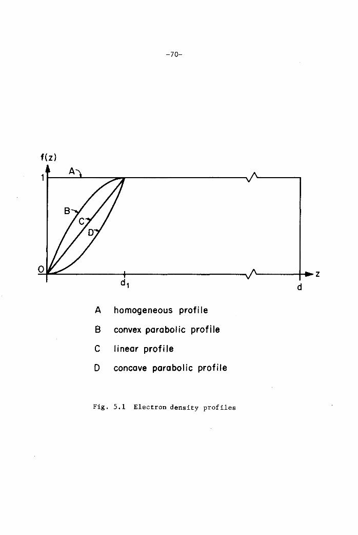
In the present report the plasma slab is chosen to have an

-69-

inhomogeneous boundary layer for 0 < z < dl and is homogeneous for

dl < z < d. Three different electron density profiles have been chosen

for the boundary layer region 0 < z < dl

. These are,

a) a convex parabolic profile,

fez)

b) a linear profile,

fez) z/d l ,

c) a concave parabolic profile,

fez)2 2

z /dl '

while fez) = 1 for dl < z < d for all three cases (Fig. 5.1). The

homogeneous plasma slab for which fez) = 1 for 0 < z < d, has also

been considered.

First, the calculations on the admittance of the circular

aperture antenna are presented. For the inhomogeneous slabs, the

input admittances YJ.'n (p) and Y. (p) have been calculated byL J.nU

numerically solving the differential equations (4.16) and (4.49) as a

function of p, while for the homogeneous case they are given by

expressions (3.27). These results have been used in the numerical

integration of expression (3.42). It is easy to see that, at least

and hence it is possible to soon terminatefor large p,

for the homogeneous plasma slab, the integrand of (3.42) is of the

-3porder of

the integration without appreciable error. The integrand has been

-70-

f(z)

1~--L.--~_r-----------~

o

A homogeneous profi Ie

B convex parabolic profile

C linear profile

o concave parabolic profile

Fig. 5.1 Electron density profiles

---~~z

d

-71-

checked for possible surface wave poles and such poles have been account-

ed for although their effect is negligible in the range of parameters

under consideration.

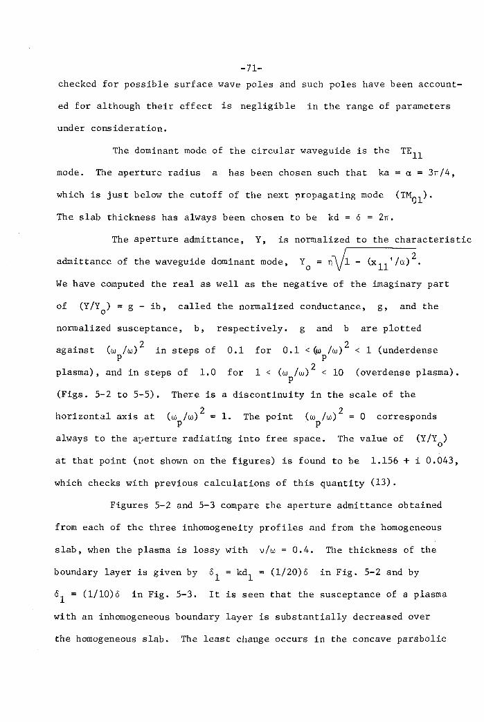
The dominant mode of the circular waveguide is the TEll

mode. The aperture radius a has been chosen such that ka = a = 3n/4,

which is just below the cutoff of the next propagating mode (TMOl)'

The slab thickness has always been chosen to be kd = °= 2n.

The aperture admittance, Y, is normalized to the characteristic

admittance of the waveguide dominant mode,Yo = n'\!l - (x ll '/a)2.

We have computed the real as well as the negative of the imaginary part

of (Y/Y) = g - ib, called the normalized conductance, g, and theo

normalized susceptance, b, respectively. g and b are plotted

2 2< I (underdenseagainst (w /w) in steps of 0.1 for 0.1 < (til /w)

p p

plasma), 1.0 2 (overdense plasma).and in steps of for 1 < (w /w) < 10p

(Figs. 5-2 to 5-5). There is a discontinuity in the scale of the

horizontal axis at 2(w /w) = 1.

pThe point 2(w /w)

po corresponds

always to the aperture radiating into free space. The value of (Y/Y )o

at that point (not shown on the figures) is found to be 1.156 + i 0.043,

which checks with previous calculations of this quantity (13).

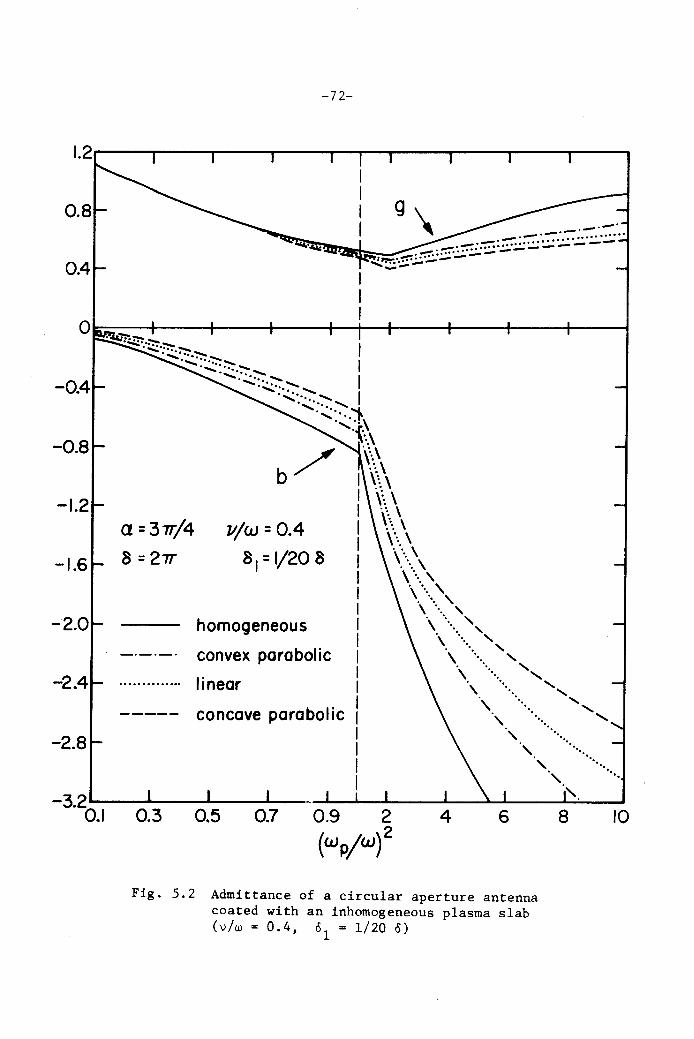
Figures 5-2 and 5-3 compare the aperture admittance obtained

from each of the three inhomogeneity profiles and from the homogeneous

slab, when the plasma is lossy with v/w = 0.4. The thickness of the

boundary layer is given by 01 = kdl

= (1/20)0 in Fig. 5-2 and by

01 = (1/10)0 in Fig. 5-3. It is seen that the susceptance of a plasma

with an inhomogeneous boundary layer is substantially decreased over

the homogeneous slab. The least change occurs in the concave parabolic

-72-

...........

........".

".

9 \ _._._.-:::-:::..~lI:I2t~-d~~ .~"o~:~ :E'::'::;.::.:.::':':".:.:."--

~~ ..~..:.:..::.:':- ----~--

v/w =0.4

81=1/20 8

homogeneous

convex parabolic

linear

(l =31T/4

8=21T

----- concave parabolic

1.2---~--r-----,.--r--r--""----,-----r--~-...,

-1.2

0.8

-1.6

-2.4

-0.8

-3.2L--..L...-.....L.----L---.L--'--~2--4.L.---..Jio......1,6--..a..-:...-~100.1 0.3 0.5 0.7 0.9

(wp/w) 2

-2.8

-2.0

Fig. 5.2 Admittance of a circular aperture antennacoated with an inhomogeneous plasma slab(v/w = 0.4, 01 = 1/20 0)

-73-

--- ..- ....".. 1""- -.--- .

.......L'.Z!::t~ •.--- ::-:: .~...~....-........ ,- -----I~ "....--- ....--

II

1.2 __-~-___r--_.__-~-:___r_-__r--~-__r_-~

0.4

0.8

lI/W =0.4

81=1/ 108

homogeneous

convex parabolic

linear

Q =37T/4

8=27T

----- concave parabolic

-1.6

-1.2

-2.0

-0.4

-2.4

-0.8

-2.8

- 3.2 ""'--_..........._---I.__~_ ___a.._L....______L. '"___~__

0.1 0.3 0.5 0.7 0.9 2 4 6 8 10

(Wp/w)2Fig. 5.3 Admittance of a circular aperture antenna

coated with an inhomogeneous plasma slab(vlw = 0.4, 01 = lila 6)

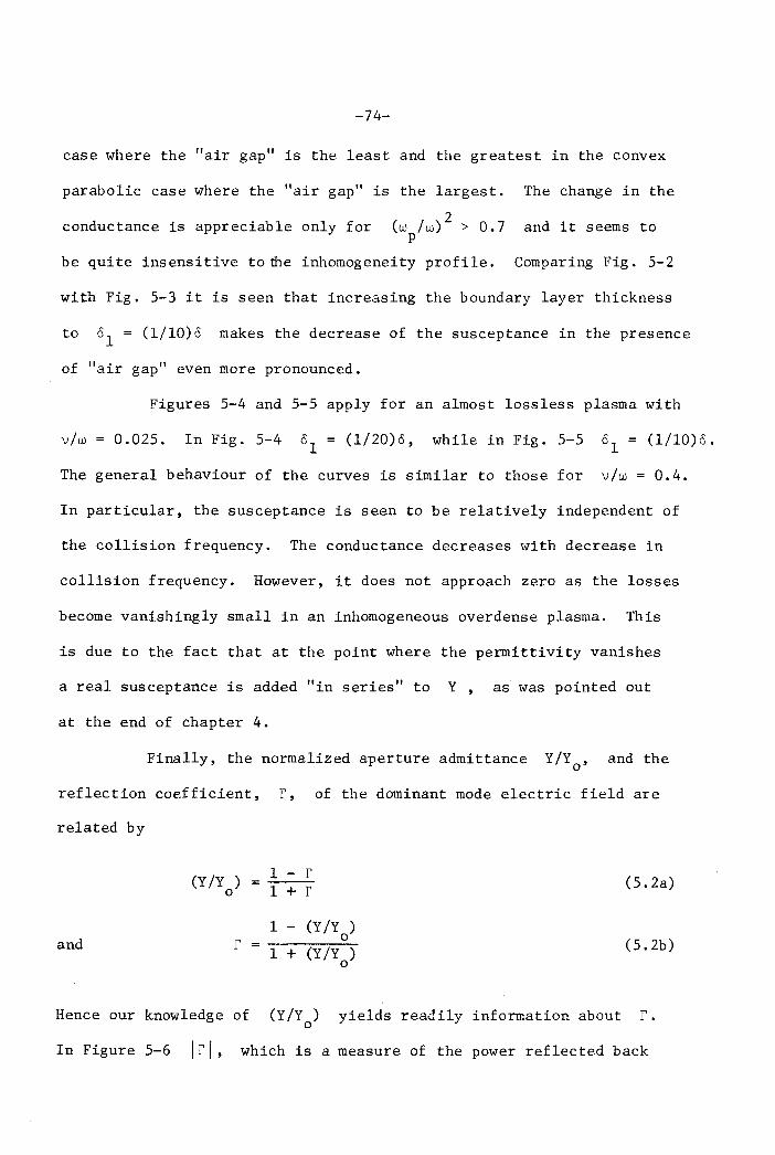
conductance is appreciable only for

-74-

case where the llair gap" is the least and the greatest in the convex

parabolic case where the "air gap" is the largest. The change in the

2(w /w) > 0.7 and it seems top

be quite insensitive tofue inhomogeneity profile. Comparing Fig. 5-2

with Fig. 5-3 it is seen that increasing the boundary layer thickness

to 01 = (1/10)0 makes the decrease of the susceptance in the presence

of "air gap" even more pronounced.

Figures 5-4 and 5-5 apply for an almost lossless plasma with

v/w 0.025. In Fig. 5-4 01 = (1/20)0, while in Fig. 5-5 01 = (1/10)0.

The general behaviour of the curves is similar to those for v/w = 0.4.

In particular, the susceptance is seen to be relatively independent of

the collision frequency. The conductance decreases with decrease in

collision frequency. However, it does not approach zero as the losses

become vanishingly small in an inhomogeneous overdense plasma. This

is due to the fact that at the point where the permittivity vanishes

a real susceptance is added "in series" to Y, as was pointed out

at the end of chapter 4.

Finally, the normalized aperture admittance Y/Yo ' and the

reflection coefficient, r, of the dominant mode electric field are

related by

(Y/Y )1 - r

=0 1 + r

1 - (Y/Y )and r 0

1 + (Y/Y )0

(5.2a)

(5.2b)

Hence our knowledge of (Y/Y) yields readily information about r.o

In Figure 5-6 Irl, which is a measure of the power reflected back

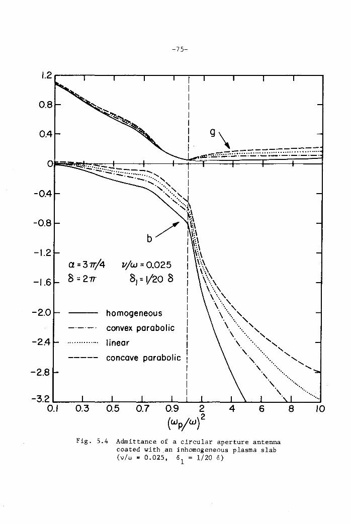
-75-

1.2 ~--r----.,.--,..---.----;----,.---..,.-----,---,---..,

g\ ----~~:E..!E:~·~-::~~0·7:.·~.:.::~·.:.:::·.

v/w =0.025

8, =V20 8

concave parabolic

homogeneous

convex parabolic

linear

a =37T/4

8=27T

o -

0.4

0.8

-0.4

-1.2

-1.6

-0.8

-2.4

-2.0

....::. -.:.:.,...::.:.'7::::- -- _.--:~ -,.-._........... I

" '.'. '.'':".' I

':~~~".J\

.\\~.~\\~\

I \~\I i\\I .\\I ~~.~I \ ..~I \'~I \.~\,....,.... ,

'. ". ,\. ..... ,\ .... ,\ ...... '," "

. '. ", ". ". '. "'. .... ,'\ ". "

" "," ".

" ." '

-3.2 '--_--L-_---L__~_---'-........L.___II.....__....Io.___~__a...__.~-- .

0.1 0.3 0.5 0.7 0.9 2 4 10

(wp/w) 2

-2.8

Fig. 5.4 Admittance of a circular aperture antennacoated with .an inhomogeneous plasma slab(vlw = 0.025, 01 = 1/20 0)

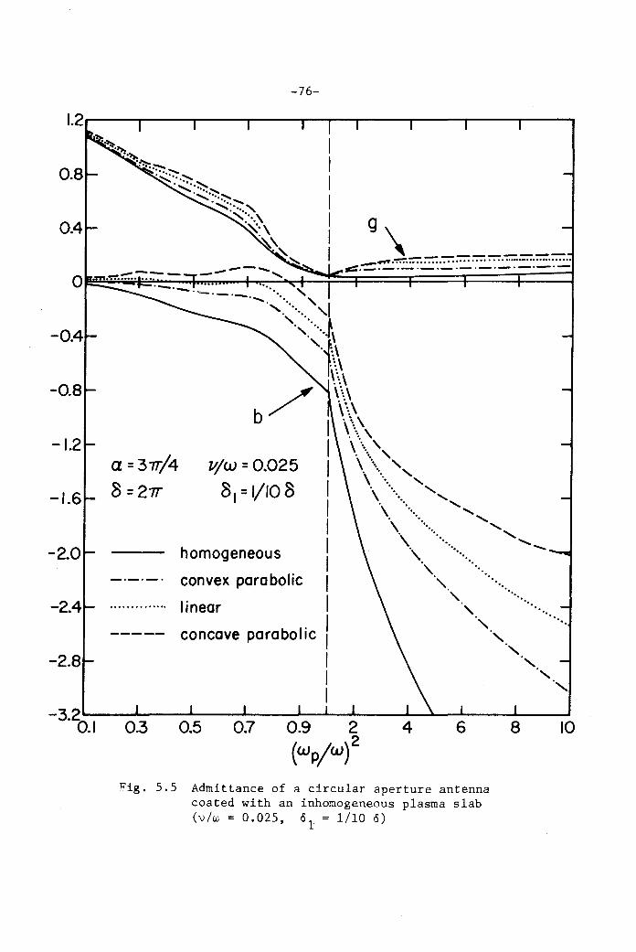
-76-

7//W =0.025

8,=1/108

homogeneous

convex parabolic

linear

a =37T/4

8=27T

9

\ --------,e::::::::::=-..::.:::::-::-:.;.- ::::.w· .::.:. : :.::.:.~=:::: ...:.::

O~~~;.=.:+==:.:..~ ~.. ~,~I~~====t======r====F=:::::::J_ ,I' 'I

'<>..},"~\'

r,~~.~\

./ '\\b / \ ....,

I \\>,I \ ..... '. ". ,I '\.'. '. ,I \. ...... "I

\. ..... ....... ......."" .......I \ .......

. ". "-I \. .... .......-\. .....I " .I ". . .I , .....

" . ".

I ". ".concave parabolic I '.

I '.,I ".I ........

-1.2

-0.4

-2.4

-O.S

-1.6

-2.S

-3.20L...I--0......3--0.....l......5--0......7--0.....L.9--.JL....-2"----......4----l1o.--'6'----.......S ----...10

(Wp/W) 2

-2.0

Fig. 5.5 Admittance of a circular aperture antennacoated with an inhomogeneous plasma slab(v/w = 0.025, 01 = 1/10 0)

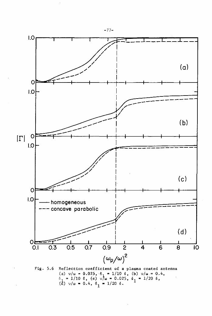
-77-

(0)

o~':::::::..::J---+--+---+--+----f--+---+--+-----11.0

(b)

(c)

----------------

I _-----I --------,/

I

_"""/",- I-'"

-- I----o - ­1.0

IfI

10

(d)

86

-----------

40.70.50.3O --a.__-"-__.....-_---I~'""""____L.___"___~_ __...& _

0.1

0~c:::2::+_-_+_-____+_-___f.~f__~-_+_-_+_-_+-____I

LO __ homogeneous--- concave parabolic

Fig. 5.6 Reflection coefficient of a plasma coated antenna(a) v/w • 0.025, -° 1 • 1/10 G, (h) v/w = 0.4,°1 = 1/10 0, (e) v/w • 0.025, 01 = 1/20 6,(0) v/w • 0.4, 01 • 1/20 o.

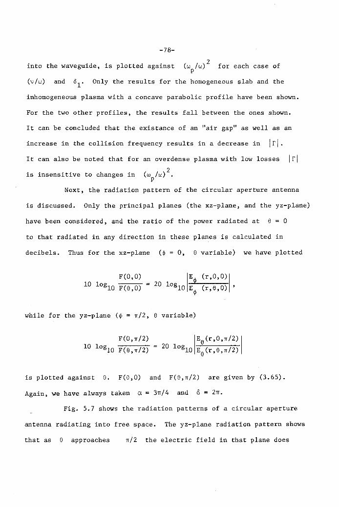
-78-

into the waveguide, is plotted against 2(w /w) for each case ofp

is insensitive to changes in

(v/w) and 01' Only the results for the homogeneous slab and the

inhomogeneous plasma with a concave parabolic profile have been shown.

For the two other profiles, the results fall between the ones shown.

It can be concluded that the existance of an "air gap" as well as an

increase in the collision frequency results in a decrease in Irl.It can also be noted that for an overdense plasma with low losses Irl

(w /w)2.p

Next, the radiation pattern of the circular aperture antenna

is discussed. Only the principal planes (the xz-plane, and the yz-plane)

have been considered, and the ratio of the power radiated at e = °to that radiated in any direction in these planes is calculated in

decibels. Thus for the xz-plane (¢ = 0, e variable) we have plotted

F(O,O)

10 loglO F(8,0) IEep (r,o,o)1

= 20 loglO E¢ (r,8,0) ,

while for the yz-plane (¢ 1T /2, e variable)

F(0,1T/2)

10 loglO F(8,1T/2)

is plotted against 8. F(8,0) and F(8,1T/2) are given by (3.65).

Again, we have always taken a = 3n/4 and 0 = 2n.

Fig. 5.7 shows the radiation patterns of a circular aperture

antenna radiating into free space. The yz-plane radiation pattern shows

that as 8 approaches 1T/2 the electric field in that plane does

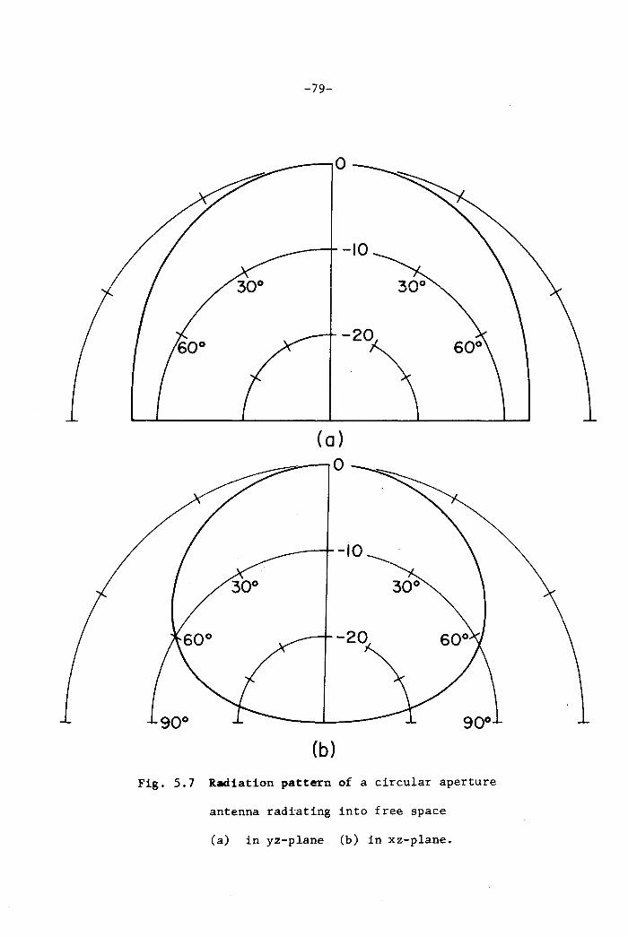
-79-

-20

-...,...-10

~;JV

----,0

(b)

Fig. 5.7 Radiation pattern of a circular aperture

antenna radiating into free space

(a) in yz-plane (b) in xz-plane.

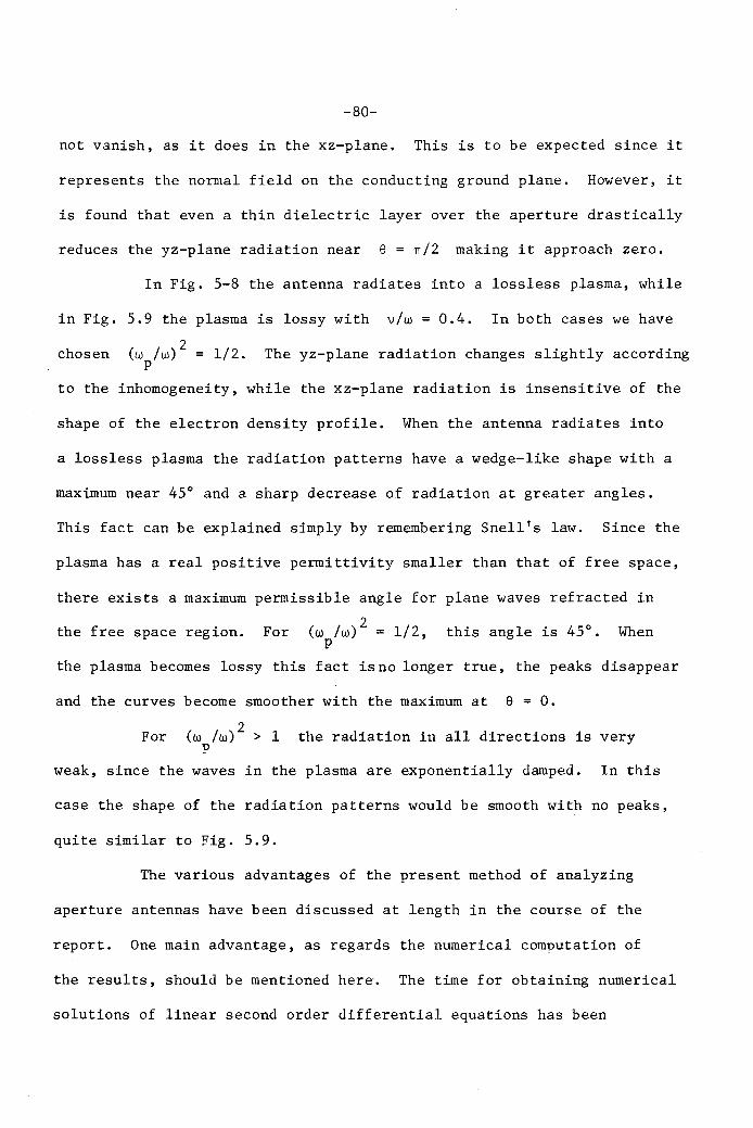
-80-

not vanish, as it does in the xz-plane. This is to be expected since it

represents the normal field on the conducting ground plane. However, it

is found that even a thin dielectric layer over the aperture drastically

reduces the yz-plane radiation near e = n/2 making it approach zero.

In Fig. 5-8 the antenna radiates into a lossless plasma, while

in Fig. 5.9 the plasma is lossy with v/w = 0.4. In both cases we haveo

chosen (w /W)L = 1/2. The yz-plane radiation changes slightly accordingp

to the inhomogeneity, while the xz-plane radiation is insensitive of the

shape of the electron density profile. When the antenna radiates into

a lossless plasma the radiation patterns have a wedge-like shape with a

maximum near 45° and a sharp decrease of radiation at greater angles.

This fact can be explained simply by remembering Snell's law. Since the

plasma has a real positive permittivity smaller than that of free space,

there exists a maximum permissible angle for plane waves refracted in

this angle is 45°. Whenthe free space region. For (w /w)2 = 1/2,P

the plasma becomes lossy this fact isno longer true, the peaks disappear

and the curves become smoother with the maximum at e = o.

For (w /w)2 > 1 the radiation in all directions is veryp

weak, since the waves in the plasma are exponentially damped. In this

case the shape of the radiation patterns would be smooth with no peaks,

quite similar to Fig. 5.9.

The various advantages of the present method of analyzing

aperture antennas have been discussed at length in the course of the

report. One main advantage, as regards the numerical computation of

the results, should be mentioned here. The time for obtaining numerical

solutions of linear second order differential equations has been

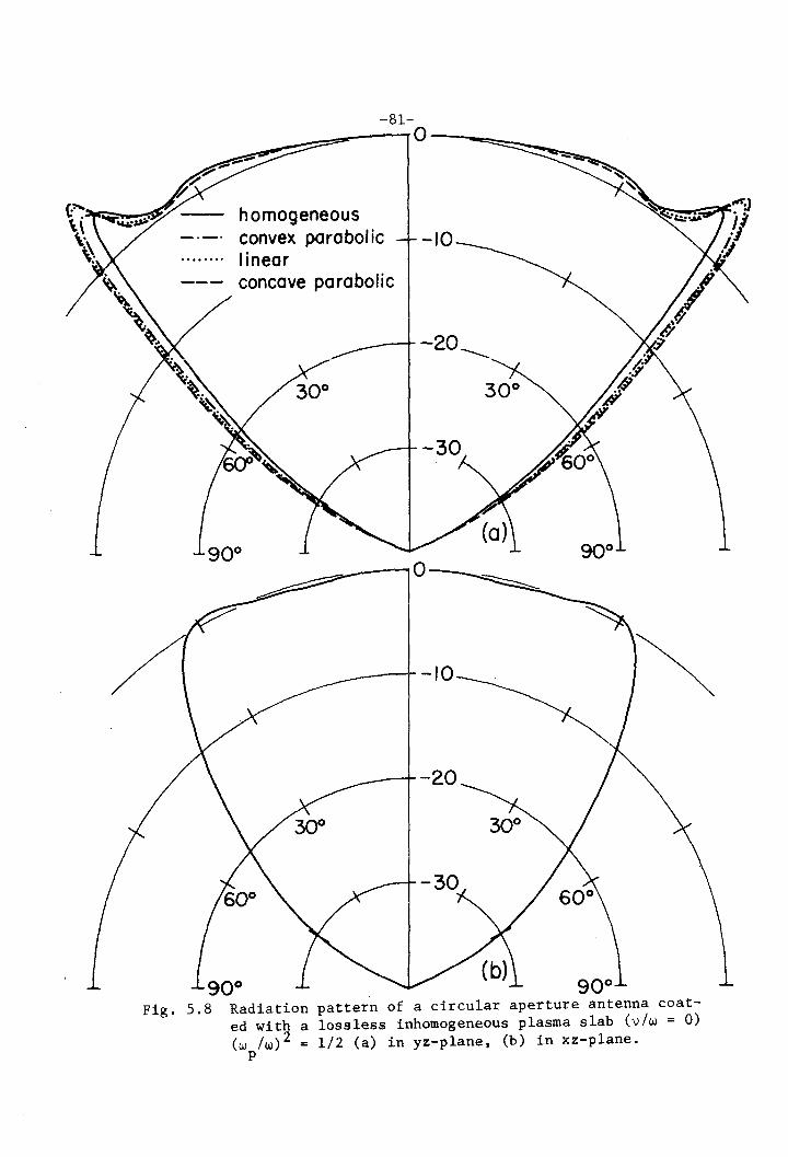
90°

---20

- ...... -20 -........

--+--10

--..... 0---~

30°

-81­~-::;:::::::::'~-IO-~~_

homogeneousconvex parabolic -10linearconcave parabolic

90°Fig. 5.8 Radiation pattern of a circular aperture antenna coat­

ed with a lossless inhomogeneous plasma slab (v/w = 0)(w /w)2 = 1/2 (a) in yz-plane, (b) in xz-plane.

p

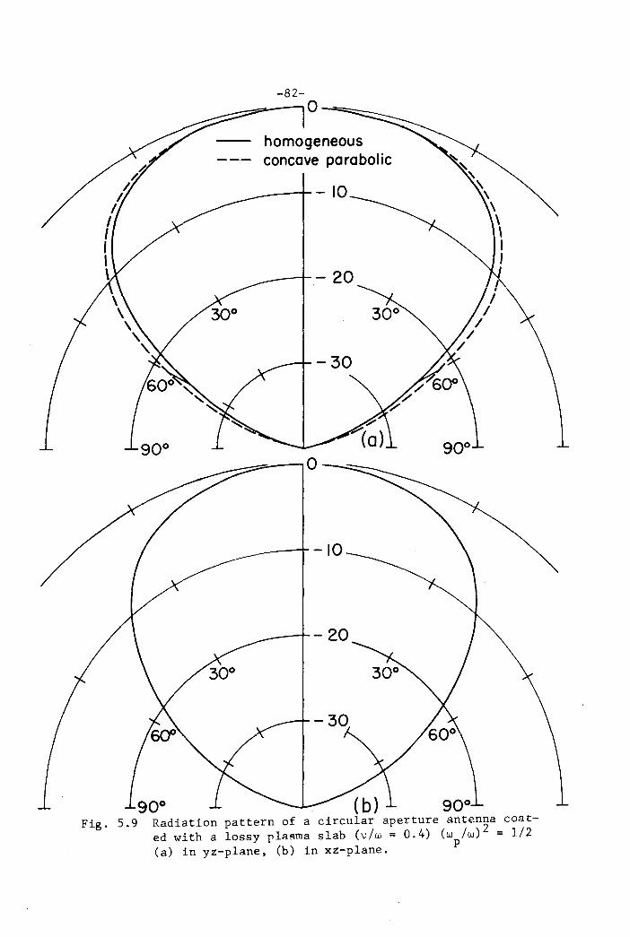
-30

--'-- 20

homogeneousconcave parabolic

~-+-- 10

-82----=-;;;;:::::::;~-,a---.:;;=:__

Fig.

__~=---, a -..;;;:;::.__

~--t--IO

(b) 90°Radiation pattern of a circular aperture antenna coat­ed with a lossy plasma slab (v/w = 0.4) (w /w)2 = 1/2(a) in yz-plane, (b) in xz-plane. P

-83-

eliminated in the present formulation. In this report we deal with non­

linear first order equations which require a far less time for solution

by a computer, than linear second order equations.

We will conclude with a discussion of the possible extensions

of the method presented. First, the method could be extended to other

than planar geometries. A treatment of cylindrical geometry, for example,

would be particularly useful for the disoussion of plasma covered

cylindrical antennas, and would be quite straightforward to carry out.

Second, the method could be used to apply to media other than the ones

discussed in this report, such as turbulent, moving and anisotropic media.

A medium whose contitutive parameters are functions of all three space

coordinates would be harder to treat, and an extension of this method

to such media mayor may not be possible.

-84­

REFERENCES

(1) Levine, H. and Schwinger, J., "On the Theory of Diffraction by an

Aperture in an Infinite Plane Screen", Part I, Phys. Rev. ~,

958-974 (1948). Part II, Phys. Rev. ]2, 1423-1432 (1949).

(2) Levine, H. and Schwinger, J., "On the Theory of Electromagnetic

Wave Diffraction by an Aperture in an Infinite Plane Conducting

Screen", Connn. Pure and Appl. Hath., 1, 355-391 (1950).

(3) Levine, H. and Papas, C. H., "Theory of the Circular Diffraction

Antenna", J. App. Phys. ~' 29-43 (1951).

(4) Lewin, L., Advanced Theory of Waveguides, Iliffe and Sons, Ltd.,

London 3 1951, pp 121-128.

(5) Galejs, J., "Slot Antenna Impedance for Plasma Layers," IEEE

Trans. Antennas and Propagation, 12, 738-745 (1964).

(6) Galejs, J., "Admittance of Annular Slot Antennas Radiating into a

Plasma Layer", Radio Science, J. Res. NBS, 68D, 317-324 (1964).

(7) Galejs, J., "Admittance of a Waveguide Radiating into Stratified

Plasma", IEEE Trans. Antennas and Propagation, 11, 64-70 (1965).

(8) Galejs, J., "Self and Mutual Admittances of Waveguides Radiating

Into Plasma Layers", Radio Science, J. Res. NBS, 69D, 179-189

(1965).

(9) Villeneuve, A. T., "Admittance of Waveguide Radiating into Plasma

Environment", IEEE Trans. Antennas and Propagation, 13, 115-121 (1965).

(10) Compton, Jr., R. T., "The Admittance of Aperture Antennas Radiating

into Lossy Media", Rept. 1691-5, Antenna Laboratory, Ohio State

University, Columbus, Ohio; 1964.

(11) Croswell, W. F., Rudduck, R. C., and Hatcher, D. M., "The

-85-

Admittance of a Rectangular Waveguide Radiating into a Dielectric

Slab", IEEE Trans. Antennas and Propagation, 15, 627-633 (1967).

(12) Fante, R. L., "Effect of Thin Plasmas on an Aperture Antenna in an

Infinite Conducting Plane", Radio Science, 1, 87-100 (1967).

(13) Bailey, M. C. and Swift, C. T., "Input Admittance of a Circular

Waveguide Aperture Covered by a Dielectric Slab", IEEE Trans.

Antennas and Propagation, 16, 386-391 (1968).

(14) Croswell, W. F., Taylor, W. C., Swift, C. T. and Cockrell, C. R.,

"The Input Admittance of a Rectangular Waveguide-Fed Aperture

Under an Inhomogeneous Plasma: Theory and Experiment", IEEE

Trans. Antennas and Propagation, 16, 475-487, (1968).

(15) Tamir, T. and Oliner, A. A., "The Influence of Complex Waves on

the Radiation Field of a Slot-Excited Plasma Layer", IRE Trans.

Antennas and Propagation 10, 55-65 (1962).

(16) Knop, C. M. and Cohn, G. 1., "Radiation From an Aperture in a

Coated Plane", Radio Science, J. Res. NBS, 68D, 363-378 (1964).

(17) Hodara, H. and Cohn, G. 1., "Radiation From a Gyro-Plasma Coated

Magnetic Line Source", IRE. Trans. Antennas and Propagation, 10,

581-593 (1962).

(18) Hodara, H., "Radiation From a Gyro-Plasma Sheathed Aperture",

IEEE Trans. Antennas and Propagation, 11, 2-12, (1963).

(19) Marcuvitz, N., Waveguide Handbook, McGraw-Hill, New York, 1951.

(20) Galejs, J. and Mentzoni, M. H., "Waveguide Admittance for

Radiation into Plasma Layers - Theory and Experiment", IEEE

Trans. Antennas and Propagation, 15, 465-470 (1967).

(21) Stratton, J. A., Electromagnetic Theory, McGraw-Hill, New York,

_86-

1941, pp 361-364.

(22) Brekhovskikh, L., Waves in Layered Media, Academic Press, New York

and London, 1960, pp 45-48.

(23) Collin, R. E., Field Theory of Guided Waves, McGraw-Hill, New York,

1960, pp 470-477.

(24) Tamir, T. and Oliner, A. A., "The Spectrum of Electromagnetic

Waves Guided by a Plasma Layer", Proc. IEEE, 21:., 317-332 (1963).

(25) Carrier, G. F., Krook, M., Pearson, C. E., Functions of a Complex

Variable, McGraw-Hill, New York, 1966, pp 272-275.

(26) Toraldo Di Francia, G., Electromagnetic Waves, Interscience

Publishers, New York, 1955, pp 36-38.

(27) Tamir, T. and Oliner, A. A., "Guided Complex \vaves, Proc. lEE

(London) ~10, 310-334 (1963).

(28) Papas, C. H., "Plane Inhomogeneous Dielectric Slab", Caltech

Antenna Laboratory Note, 1954.

(29) Bellman, R. and Kalaba, R., "On the Principle of Invariant Im­

bedding and Propagation through Inhomogeneous Media", Proc. Nat.

Acad. Sci. USA~, 629-632 (1956).

(30) Bellman, R. and Kalaba, R., "Invariant Imbedding and Wave Pro­

pagation in Stochastic Media", Electromagnetic Wave Propagation,

edited by Desirant and Michiels, Academic Press, 1960, pp 243-252.

(31) Brekhovskikh, L., Waves in Layered Media, Academic Press, New York

and London, 1960, pp 215-218.