Embed Size (px)
Citation preview
Institute of Police Technology and Management
Analysis of Four Staged Crashes of
Passenger Vehicles into a
Semi-Trailer
Jeremy Daily
Russell Strickland
Special Problems in Traffic Crash Reconstruction
25-29 April 2005
1 Introduction
1.1 Purpose
The purpose of this report is to show the details of traffic crash reconstruction tech-
niques as applied to crashes between commercial vehicles and passenger vehicles.
There were four test conducted: two offset under-ride collisions and two crashes
into the rear duals of a stationary semitrailer. These tests were instrumented which
enables verification of the reconstruction. However, the authors did not use the in-
strumented data until after the reconstruction was finished. This removed the temp-
tation to “fudge” numbers to make the reconstruction fit the data. Furthermore, the
1
1 Introduction
use of some assumptions can be verified because we have known speeds from radar
trace of the bullet vehicle going into the target.
1.2 Testing Procedure
There were four tests performed in two days. Engineers from MacInnis Engineering
used a tow cable system to pull the bullet vehicles into the trailer. The tow cable was
fed through the center of the rear duals for two crashes and along the right and left
side for the other two crashes.
The tractor trailer was common to all crashes. The trailer was a Pine 48 ft box
van with sliding tandems. The tractor was a 2004 Mack single axle day cab (VIN:
1M1AE02YX4N00138).
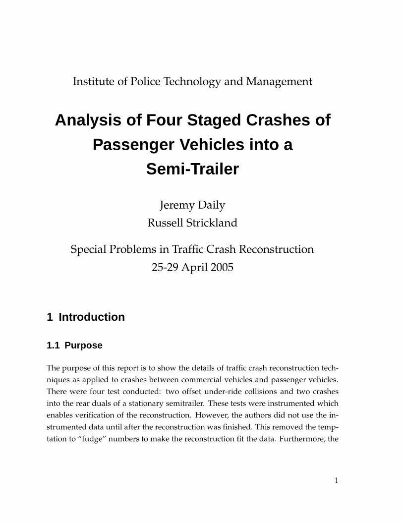
Rear Under-ride Crash #1 A 1989 Plymouth Voyager SE (VIN: 2P4FH4531KR174080)
was pulled into a stationary tractor trailer, Figure 1. It was pulled into the left rear
of the box van trailer and penetrated to the rear tires of the trailer. The tractor-trailer
combination had its spring brakes applied and was pushed forward a small amount
due to the impact.
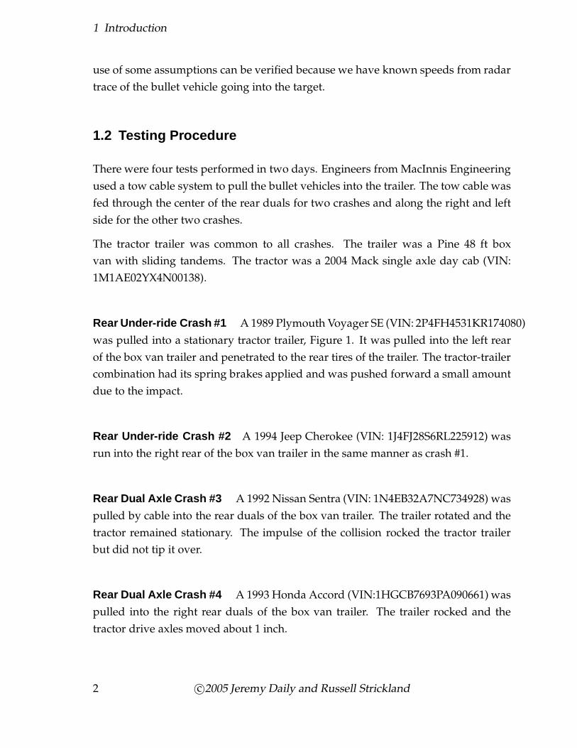
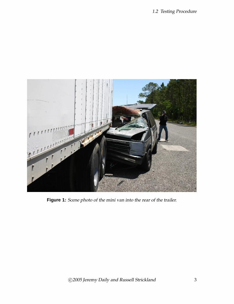
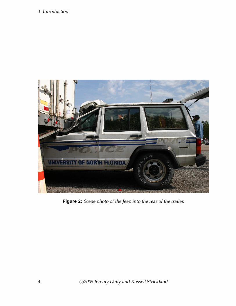
Rear Under-ride Crash #2 A 1994 Jeep Cherokee (VIN: 1J4FJ28S6RL225912) was
run into the right rear of the box van trailer in the same manner as crash #1.
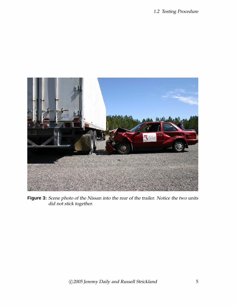
Rear Dual Axle Crash #3 A 1992 Nissan Sentra (VIN: 1N4EB32A7NC734928) was
pulled by cable into the rear duals of the box van trailer. The trailer rotated and the
tractor remained stationary. The impulse of the collision rocked the tractor trailer
but did not tip it over.
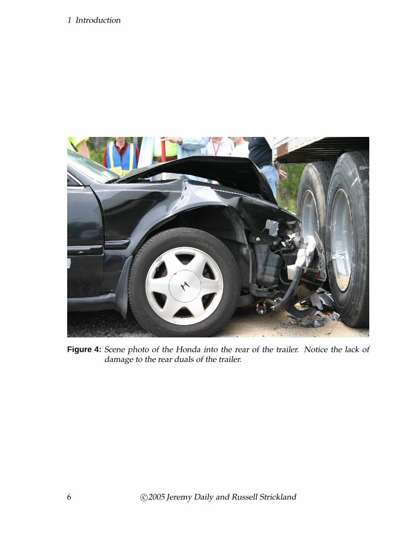
Rear Dual Axle Crash #4 A 1993 Honda Accord (VIN:1HGCB7693PA090661) was
pulled into the right rear duals of the box van trailer. The trailer rocked and the
tractor drive axles moved about 1 inch.
2 c©2005 Jeremy Daily and Russell Strickland
1.2 Testing Procedure
Figure 1: Scene photo of the mini van into the rear of the trailer.
c©2005 Jeremy Daily and Russell Strickland 3
1 Introduction
Figure 2: Scene photo of the Jeep into the rear of the trailer.
4 c©2005 Jeremy Daily and Russell Strickland
1.2 Testing Procedure
Figure 3: Scene photo of the Nissan into the rear of the trailer. Notice the two unitsdid not stick together.
c©2005 Jeremy Daily and Russell Strickland 5
1 Introduction
Figure 4: Scene photo of the Honda into the rear of the trailer. Notice the lack ofdamage to the rear duals of the trailer.
6 c©2005 Jeremy Daily and Russell Strickland

In all the tests, the a cable broke at the junction between the steel cable and the
polypropylene ski rope. The impulse required to snap the rope has no measurable
effect on the collision.
The next section presents a review of the physics used in the reconstruction of the
aforementioned collisions. A list of all the evidence should provide guidance for the
investigating accident reconstructionist. As with any collision analysis, the evidence
is the single most important factor in determining the success of the outcome of the
reconstruction. Following the reconstruction, the instrumented data is presented to
validate some of the assumptions we make during a crash reconstruction.
2 Reconstruction of Staged Crashes
2.1 Evidence Required
2.1.1 Drag Factor For Tractor Trailer
The surface of the test site was level. Skid tests with passenger vehicles give a drag
factor of 0.75 (±0.05). Since the tractor trailer has commercial vehicle tires, the drag
factor is reduced by a factor of 0.80 to compute a drag factor of
fCV = n fcar = 0.80(0.75) = 0.60
where n is the commercial vehicle tire factor.
This drag factor for the truck was verified by performing instrumented skid tests
from 30 mph with the same tractor trailer unit on the same surface of the crash tests.
The drag factor was computed using
f =S2
30d
Where d is the skid distance that includes the shadow marks. Speed was estimated
from the speedometer (undesirable) or integrated from an accelerometer trace when
available. The data are summarized in Table 1. A prudent range to use in the drag
factor for the rear tires would be from 0.55 to 0.65 based on these tests.
c©2005 Jeremy Daily and Russell Strickland 7
2 Reconstruction of Staged Crashes
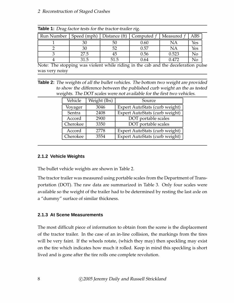
Table 1: Drag factor tests for the tractor-trailer rig.
Run Number Speed (mph) Distance (ft) Computed f Measured f ABS
1 30 50 0.60 NA Yes2 30 52 0.57 NA Yes3 27.5 45 0.56 0.523 No4 31.5 51.5 0.64 0.472 No
Note: The stopping was violent while riding in the cab and the deceleration pulsewas very noisy
Table 2: The weights of all the bullet vehicles. The bottom two weight are providedto show the difference between the published curb weight an the as testedweights. The DOT scales were not available for the first two vehicles.
Vehicle Weight (lbs) Source
Voyager 3046 Expert AutoStats (curb weight)Sentra 2408 Expert AutoStats (curb weight)Accord 2900 DOT portable scales
Cherokee 3350 DOT portable scales
Accord 2778 Expert AutoStats (curb weight)Cherokee 3554 Expert AutoStats (curb weight)
2.1.2 Vehicle Weights
The bullet vehicle weights are shown in Table 2.
The tractor trailer was measured using portable scales from the Department of Trans-
portation (DOT). The raw data are summarized in Table 3. Only four scales were
available so the weight of the trailer had to be determined by resting the last axle on
a “dummy” surface of similar thickness.
2.1.3 At Scene Measurements
The most difficult piece of information to obtain from the scene is the displacement
of the tractor trailer. In the case of an in-line collision, the markings from the tires
will be very faint. If the wheels rotate, (which they may) then speckling may exist
on the tire which indicates how much it rolled. Keep in mind this speckling is short
lived and is gone after the tire rolls one complete revolution.
8 c©2005 Jeremy Daily and Russell Strickland
2.1 Evidence Required
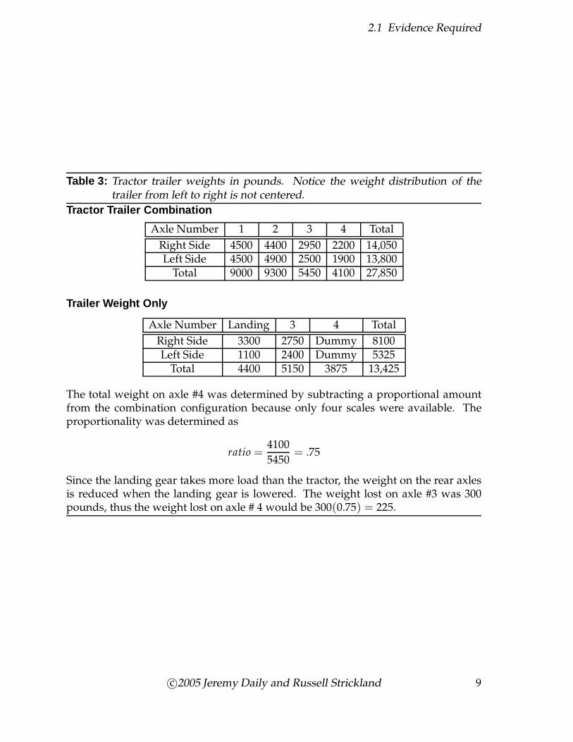
Table 3: Tractor trailer weights in pounds. Notice the weight distribution of thetrailer from left to right is not centered.
Tractor Trailer Combination
Axle Number 1 2 3 4 Total
Right Side 4500 4400 2950 2200 14,050Left Side 4500 4900 2500 1900 13,800
Total 9000 9300 5450 4100 27,850
Trailer Weight Only
Axle Number Landing 3 4 Total
Right Side 3300 2750 Dummy 8100Left Side 1100 2400 Dummy 5325
Total 4400 5150 3875 13,425
The total weight on axle #4 was determined by subtracting a proportional amountfrom the combination configuration because only four scales were available. Theproportionality was determined as
ratio =4100
5450= .75
Since the landing gear takes more load than the tractor, the weight on the rear axlesis reduced when the landing gear is lowered. The weight lost on axle #3 was 300pounds, thus the weight lost on axle # 4 would be 300(0.75) = 225.
c©2005 Jeremy Daily and Russell Strickland 9

2 Reconstruction of Staged Crashes
Figure 5: This photo illustrates the markings left by the rear duals on the pavement.The mark existed under the trailer and gives an amount the rear axles weredisplaced.
10 c©2005 Jeremy Daily and Russell Strickland
2.1 Evidence Required
For our crash test, the wheel positions were marked before and after the collision.
This enables us to accurately record the actual tire displacements of the tractor-trailer.
In the side collisions, the best evidence will be under the trailer as created by the
opposite duals as shown in Figure 5. The same types of evidence should exist for
smaller scale collisions, such as a motorcycle into a pickup. The initial and final
positions of the trailer are important for the reconstruction.
2.1.4 Physical Properties of the Trailer
We need to use the weights, along with the physical dimensions, to determine the
location of the center of mass. The height of the center of mass is not relevant to our
analysis. All calculations assume planar motion with no slope in relation to gravity.
Center of Mass of the Trailer The center of mass of any object is computed using
the formula
dCM =∑
ni=1 diwi
wTotal
where n is the number of weight forces
dCM is the distance the center of mass is from from a reference point
di is the perpendicular distance the ith force (wi) is acting from the refer-
ence point
wTotal is the total weight
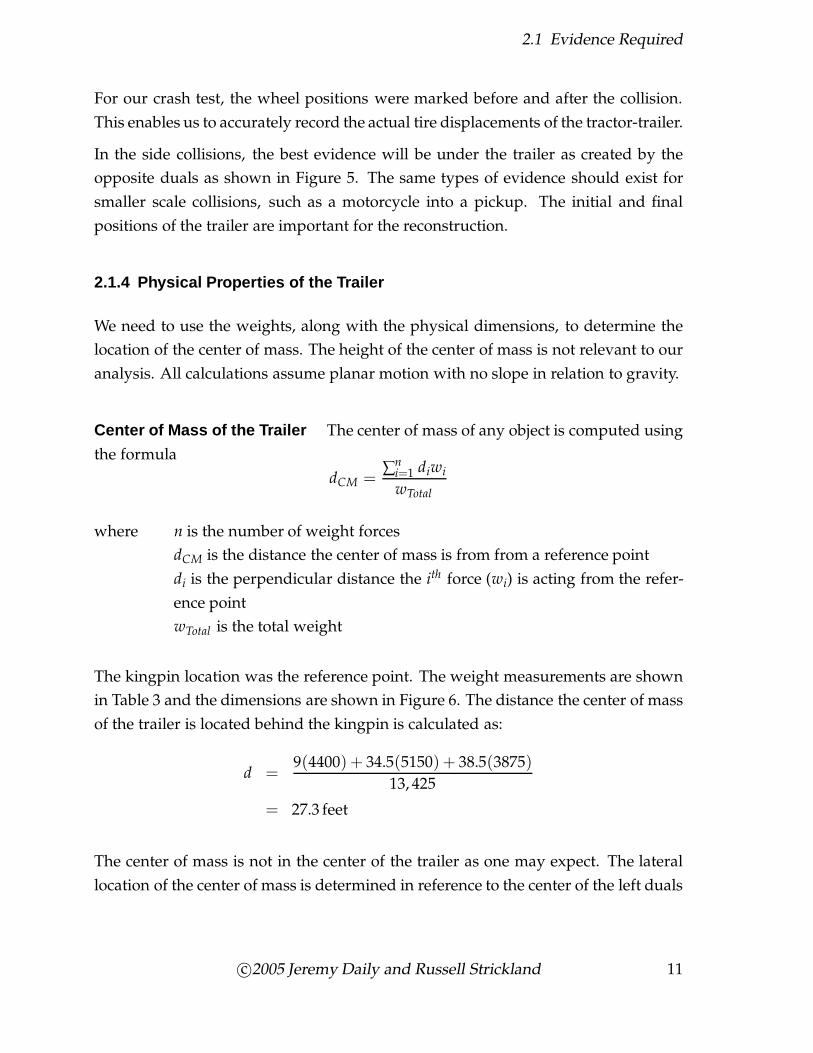
The kingpin location was the reference point. The weight measurements are shown
in Table 3 and the dimensions are shown in Figure 6. The distance the center of mass
of the trailer is located behind the kingpin is calculated as:
d =9(4400) + 34.5(5150) + 38.5(3875)
13, 425
= 27.3 feet
The center of mass is not in the center of the trailer as one may expect. The lateral
location of the center of mass is determined in reference to the center of the left duals
c©2005 Jeremy Daily and Russell Strickland 11
2 Reconstruction of Staged Crashes
Figure 6: A side view of the trailer used in the crash tests.
as shown in Figure 7. The formula to determine the distance the center of mass is
from the left duals is
dL = tw
(wR
wT
)
where tw = dL + dR is the track width. Substituting the data from Table 3 along with
a 68 inch track width for the trailer gives:
dL = 68
(5325
8100
)
= 44.7 inches
Yaw Moment of Inertia There are few ways of determining the mass moment of
inertia. The first, and easiest, is to look up the value in a database. The following
information is from Fancher, P.S., et al., DOT HS 807 125, “A Factbook of the Mechanical
Properties of the Components for Single Unit and Articulated Heavy Trucks”, December
1986:
IG = 110, 739 lb-ft-sec2
for an empty 48 ft box van trailer that weighs 13,800 lbs. The subscript G indicates
the moment of inertia assumes rotation about the center of gravity.
If the location of rotation is different from the center of mass, then, by the parallel axis
12 c©2005 Jeremy Daily and Russell Strickland

2.1 Evidence Required
Figure 7: A rear view of the trailer used to determine its center of mass.
c©2005 Jeremy Daily and Russell Strickland 13
2 Reconstruction of Staged Crashes
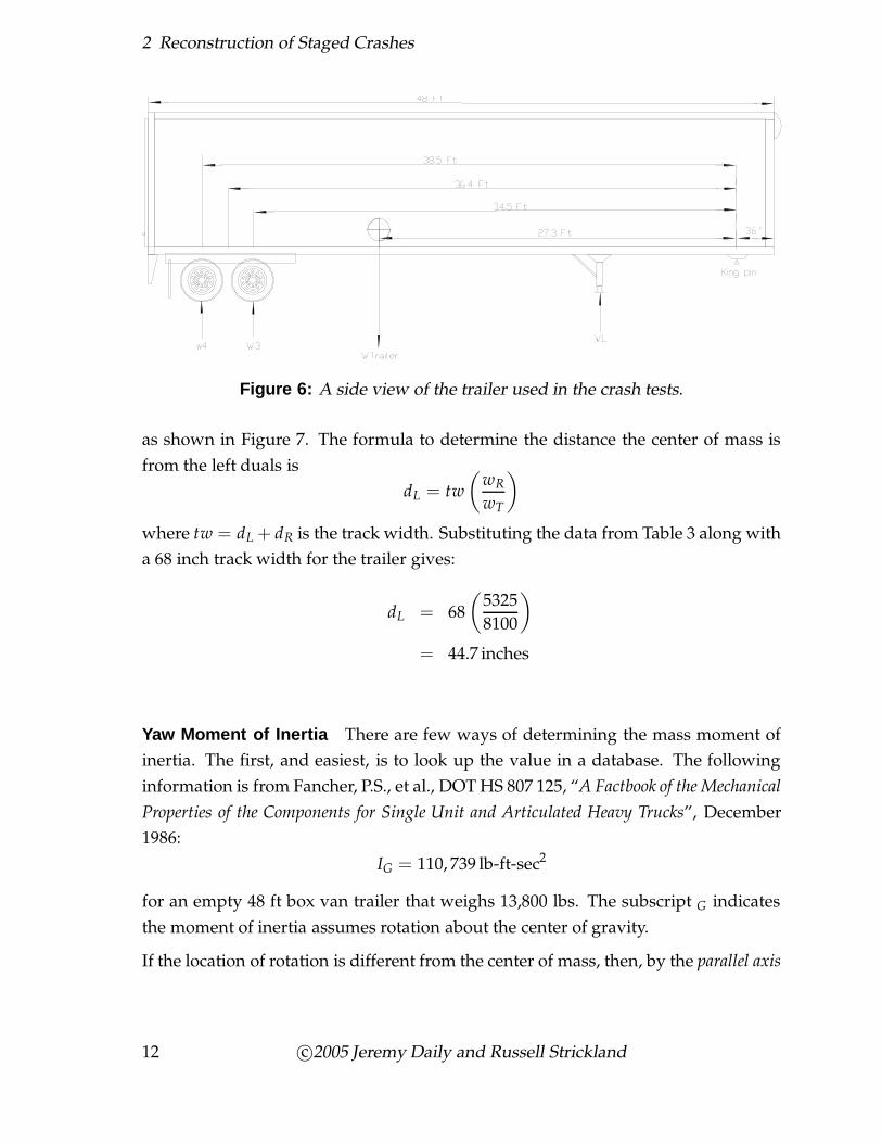
Figure 8: A top view of the trailer used to determine its center of mass.
theorem, the yaw moment of inertia changes to
I = IG + mh2
where I is the yaw moment of inertia about the point of rotation
IG is the mass moment of inertia about the center of mass
m is the mass of the object
h is the distance from the center of mass to the point of rotation
The center of mass of the trailer is slightly off center, but not enough to make a dif-
ference when computing the value of h using the Pythagorean Theorem. The value
of h, as seen in Figure 8, is 27.3 feet. So, by the parallel axis theorem,
I = IG +
(wT
g
)
h2
= 110, 739 +
(13, 425
32.2
)
27.32
= 421, 470 lb-ft-sec2
The next way to determine the mass moment of inertia is by assuming simple shapes
with uniform density. The individual objects each have a simple formula for the yaw
moment of inertia and the yaw moment of inertia for the composite structure can be
determined by using the parallel axis theorem. This technique requires practice and
time to become comfortable with the calculations.
The most reliable way (and expensive) it to measure the dynamic response of the
14 c©2005 Jeremy Daily and Russell Strickland
2.2 Under-ride Analysis Using Momentum
Fc1Fc2
Unit 2 Unit 1
m1a1m2a2
Fg Positive Direction
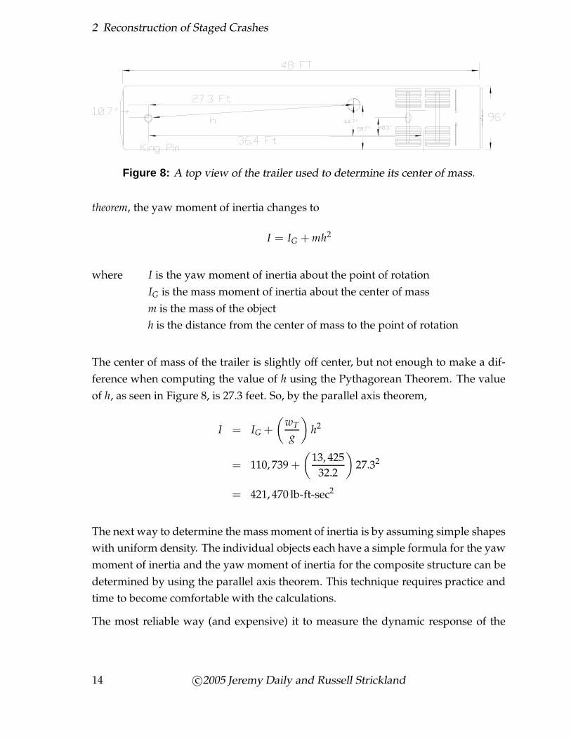
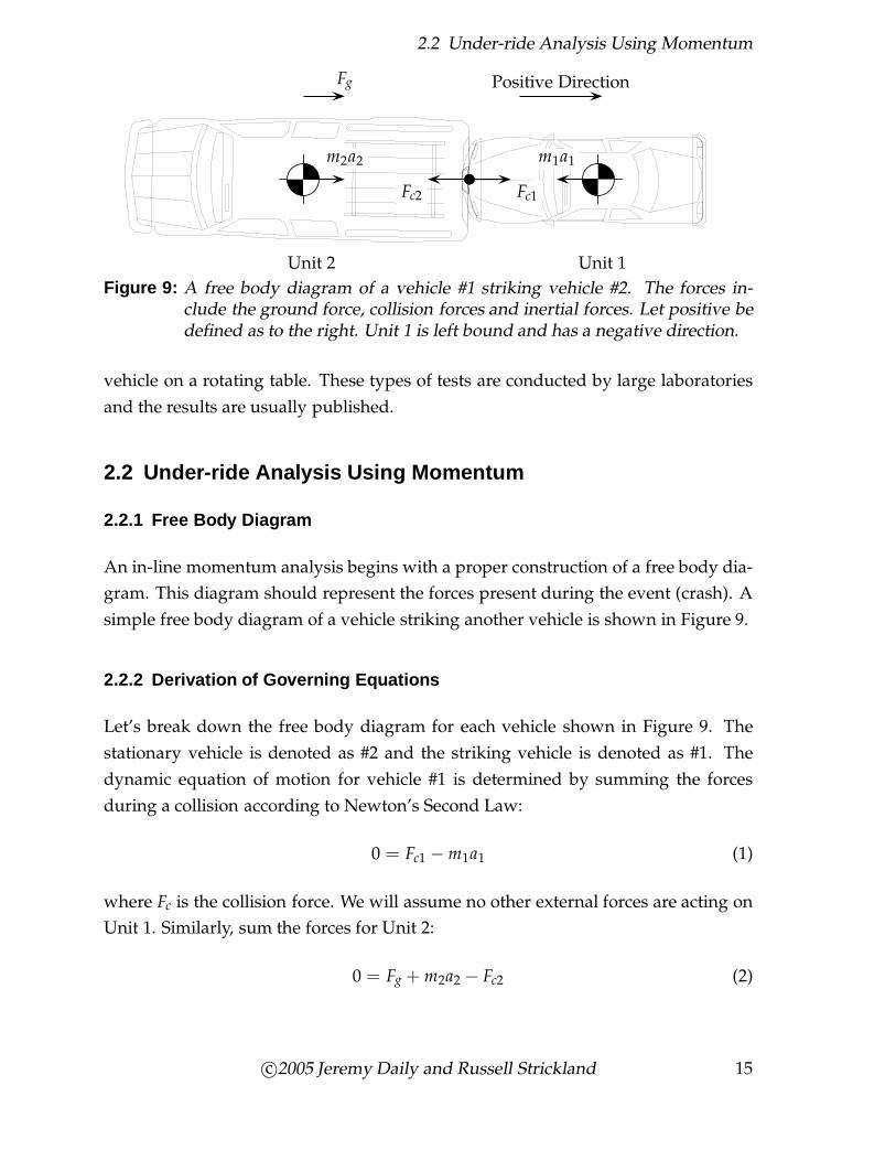
Figure 9: A free body diagram of a vehicle #1 striking vehicle #2. The forces in-clude the ground force, collision forces and inertial forces. Let positive bedefined as to the right. Unit 1 is left bound and has a negative direction.
vehicle on a rotating table. These types of tests are conducted by large laboratories
and the results are usually published.
2.2 Under-ride Analysis Using Momentum
2.2.1 Free Body Diagram
An in-line momentum analysis begins with a proper construction of a free body dia-
gram. This diagram should represent the forces present during the event (crash). A
simple free body diagram of a vehicle striking another vehicle is shown in Figure 9.
2.2.2 Derivation of Governing Equations
Let’s break down the free body diagram for each vehicle shown in Figure 9. The
stationary vehicle is denoted as #2 and the striking vehicle is denoted as #1. The
dynamic equation of motion for vehicle #1 is determined by summing the forces
during a collision according to Newton’s Second Law:
0 = Fc1 − m1a1 (1)
where Fc is the collision force. We will assume no other external forces are acting on
Unit 1. Similarly, sum the forces for Unit 2:
0 = Fg + m2a2 − Fc2 (2)
c©2005 Jeremy Daily and Russell Strickland 15
2 Reconstruction of Staged Crashes
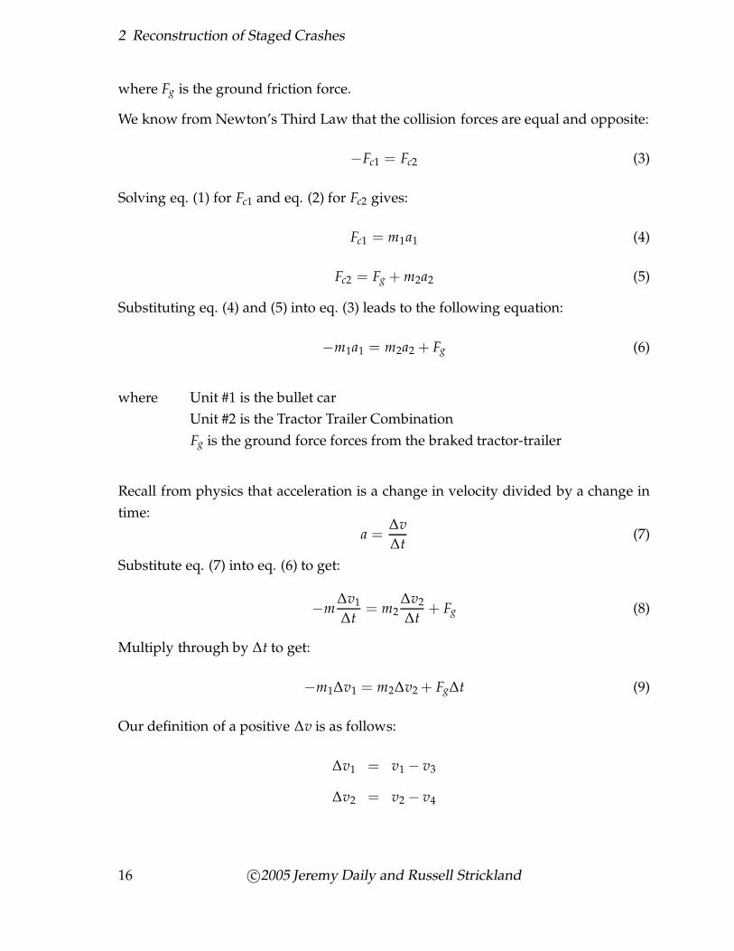
where Fg is the ground friction force.
We know from Newton’s Third Law that the collision forces are equal and opposite:
−Fc1 = Fc2 (3)
Solving eq. (1) for Fc1 and eq. (2) for Fc2 gives:
Fc1 = m1a1 (4)
Fc2 = Fg + m2a2 (5)
Substituting eq. (4) and (5) into eq. (3) leads to the following equation:
−m1a1 = m2a2 + Fg (6)
where Unit #1 is the bullet car
Unit #2 is the Tractor Trailer Combination
Fg is the ground force forces from the braked tractor-trailer
Recall from physics that acceleration is a change in velocity divided by a change in
time:
a =∆v
∆t(7)
Substitute eq. (7) into eq. (6) to get:
−m∆v1
∆t= m2
∆v2
∆t+ Fg (8)
Multiply through by ∆t to get:
−m1∆v1 = m2∆v2 + Fg∆t (9)
Our definition of a positive ∆v is as follows:
∆v1 = v1 − v3
∆v2 = v2 − v4
16 c©2005 Jeremy Daily and Russell Strickland
2.2 Under-ride Analysis Using Momentum
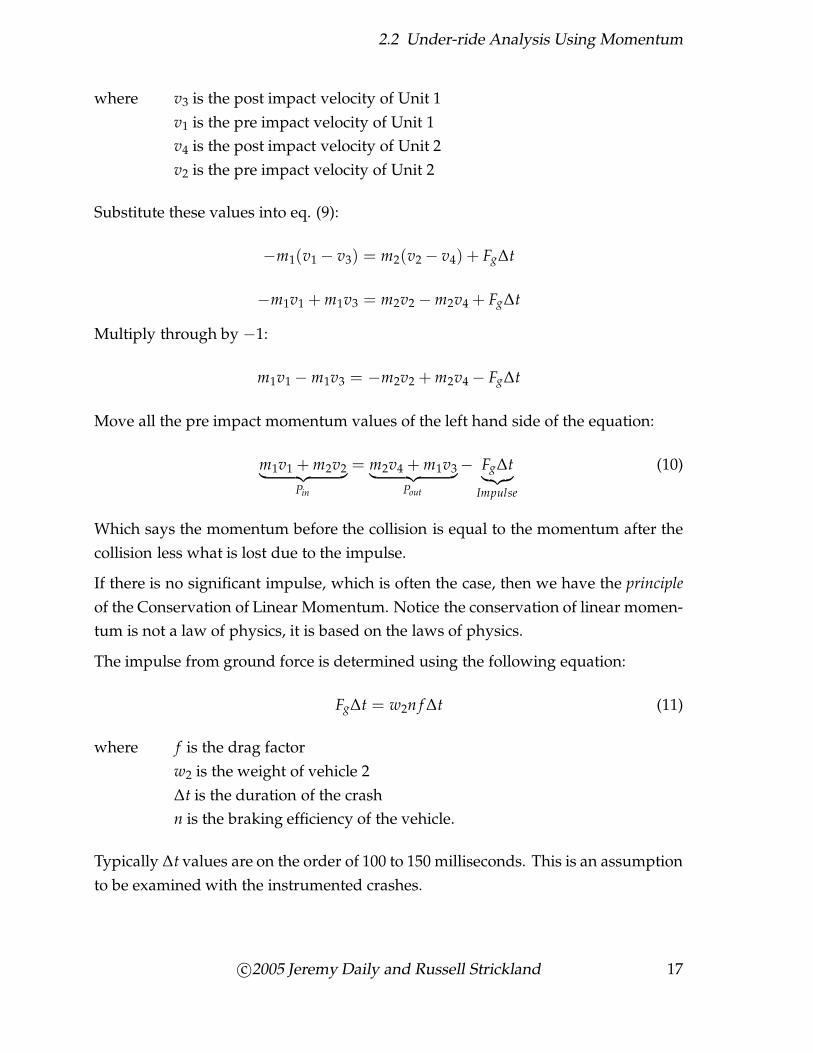
where v3 is the post impact velocity of Unit 1
v1 is the pre impact velocity of Unit 1
v4 is the post impact velocity of Unit 2
v2 is the pre impact velocity of Unit 2
Substitute these values into eq. (9):
−m1(v1 − v3) = m2(v2 − v4) + Fg∆t
−m1v1 + m1v3 = m2v2 − m2v4 + Fg∆t
Multiply through by −1:
m1v1 − m1v3 = −m2v2 + m2v4 − Fg∆t
Move all the pre impact momentum values of the left hand side of the equation:
m1v1 + m2v2︸ ︷︷ ︸
Pin
= m2v4 + m1v3︸ ︷︷ ︸
Pout
− Fg∆t︸︷︷︸
Impulse
(10)
Which says the momentum before the collision is equal to the momentum after the
collision less what is lost due to the impulse.
If there is no significant impulse, which is often the case, then we have the principle
of the Conservation of Linear Momentum. Notice the conservation of linear momen-
tum is not a law of physics, it is based on the laws of physics.
The impulse from ground force is determined using the following equation:
Fg∆t = w2n f ∆t (11)
where f is the drag factor
w2 is the weight of vehicle 2
∆t is the duration of the crash
n is the braking efficiency of the vehicle.
Typically ∆t values are on the order of 100 to 150 milliseconds. This is an assumption
to be examined with the instrumented crashes.
c©2005 Jeremy Daily and Russell Strickland 17
2 Reconstruction of Staged Crashes
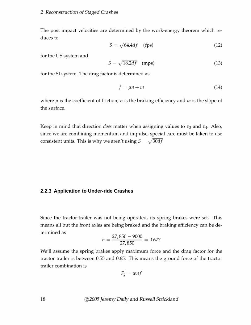
The post impact velocities are determined by the work-energy theorem which re-
duces to:
S =√
64.4d f (fps) (12)
for the US system and
S =√
18.2d f (mps) (13)
for the SI system. The drag factor is determined as
f = µn + m (14)
where µ is the coefficient of friction, n is the braking efficiency and m is the slope of
the surface.
Keep in mind that direction does matter when assigning values to v3 and v4. Also,
since we are combining momentum and impulse, special care must be taken to use
consistent units. This is why we aren’t using S =√
30d f
2.2.3 Application to Under-ride Crashes
Since the tractor-trailer was not being operated, its spring brakes were set. This
means all but the front axles are being braked and the braking efficiency can be de-
termined as
n =27, 850 − 9000
27, 850= 0.677
We’ll assume the spring brakes apply maximum force and the drag factor for the
tractor trailer is between 0.55 and 0.65. This means the ground force of the tractor
trailer combination is
Fg = wn f
18 c©2005 Jeremy Daily and Russell Strickland
2.2 Under-ride Analysis Using Momentum
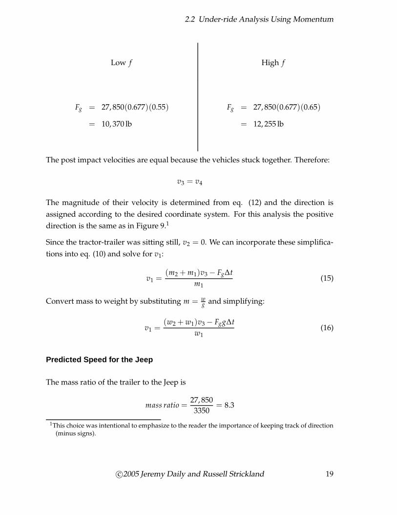
Low f High f
Fg = 27, 850(0.677)(0.55)
= 10, 370 lb
Fg = 27, 850(0.677)(0.65)
= 12, 255 lb
The post impact velocities are equal because the vehicles stuck together. Therefore:
v3 = v4
The magnitude of their velocity is determined from eq. (12) and the direction is
assigned according to the desired coordinate system. For this analysis the positive
direction is the same as in Figure 9.1
Since the tractor-trailer was sitting still, v2 = 0. We can incorporate these simplifica-
tions into eq. (10) and solve for v1:
v1 =(m2 + m1)v3 − Fg∆t
m1(15)
Convert mass to weight by substituting m = wg and simplifying:
v1 =(w2 + w1)v3 − Fgg∆t
w1(16)
Predicted Speed for the Jeep
The mass ratio of the trailer to the Jeep is
mass ratio =27, 850
3350= 8.3
1This choice was intentional to emphasize to the reader the importance of keeping track of direction(minus signs).
c©2005 Jeremy Daily and Russell Strickland 19

2 Reconstruction of Staged Crashes
The Jeep displaced the tractor-trailer 1.5 ft. Hence, the post impact velocity can be
computed using a low and high drag factor:
Low f High f
v3 = −
√
64.4(1.5)(0.677)(0.55)
= −6.00 fps
v3 = −
√
64.4(1.5)(0.677)(0.65)
= −6.52 fps
The post impact velocity is negative (left bound) according to our positive sign con-
vention.2
Substitute the appropriate values for the Jeep striking the tractor trailer:
Low f , No ∆t:
v1 =(27, 850 + 3350)(−6.00)− 10, 370(32.2)(0)
3350
v1 = −55.88 fps
S1 = 38.1 mph
High f , High ∆t:
v1 =(27, 850 + 3350)(−6.52)− 12, 255(32.2)(0.100)
3350
v1 = −72.5 fps
S1 = 49.4 mph
2Accelerometer data suggest v3 = 4.7 fps is a better number for the post impact speed of the tractor-trailer.
20 c©2005 Jeremy Daily and Russell Strickland
2.2 Under-ride Analysis Using Momentum
Both speeds are in the negative direction. Our predicted speeds based on ranging
the drag factor for the truck and the magnitude of the external impulse are between
38 and 49 mph.3
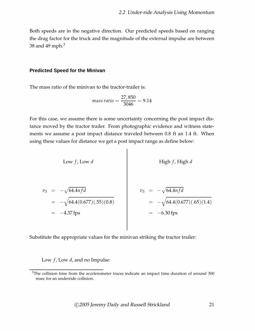
Predicted Speed for the Minivan
The mass ratio of the minivan to the tractor-trailer is:
mass ratio =27, 850
3046= 9.14
For this case, we assume there is some uncertainty concerning the post impact dis-
tance moved by the tractor trailer. From photographic evidence and witness state-
ments we assume a post impact distance traveled between 0.8 ft an 1.4 ft. When
using these values for distance we get a post impact range as define below:
Low f , Low d High f , High d
v3 = −√
64.4n f d
= −
√
64.4(0.677)(.55)(0.8)
= −4.37 fps
v3 = −√
64.4n f d
= −
√
64.4(0.677)(.65)(1.4)
= −6.30 fps
Substitute the appropriate values for the minivan striking the tractor trailer:
Low f , Low d, and no Impulse:
3The collision time from the accelerometer traces indicate an impact time duration of around 300msec for an underride collision.
c©2005 Jeremy Daily and Russell Strickland 21
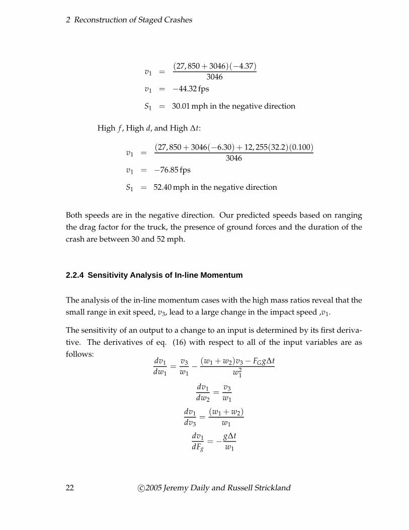
2 Reconstruction of Staged Crashes
v1 =(27, 850 + 3046)(−4.37)
3046
v1 = −44.32 fps
S1 = 30.01 mph in the negative direction
High f , High d, and High ∆t:
v1 =(27, 850 + 3046(−6.30) + 12, 255(32.2)(0.100)
3046
v1 = −76.85 fps
S1 = 52.40 mph in the negative direction
Both speeds are in the negative direction. Our predicted speeds based on ranging
the drag factor for the truck, the presence of ground forces and the duration of the
crash are between 30 and 52 mph.
2.2.4 Sensitivity Analysis of In-line Momentum
The analysis of the in-line momentum cases with the high mass ratios reveal that the
small range in exit speed, v3, lead to a large change in the impact speed ,v1.
The sensitivity of an output to a change to an input is determined by its first deriva-
tive. The derivatives of eq. (16) with respect to all of the input variables are as
follows:dv1
dw1=
v3
w1−
(w1 + w2)v3 − FGg∆t
w21
dv1
dw2=
v3
w1
dv1
dv3=
(w1 + w2)
w1
dv1
dFg= −
g∆t
w1
22 c©2005 Jeremy Daily and Russell Strickland
2.3 Eccentric Collision Analysis Using Rotational Mechanics
dv1
d∆t= −
gFg
w1
These formulas provide a tool to analytically determine how sensitive each input
variable is to the resulting output (v1). Substitution of the values used in the analysis
herein would reveal that the v1 determination is sensitive to ∆t, w1 and v3. Therefore,
any uncertainty in these values is amplified in the determination of the impact speed.
This is why there is a large range for v1 for a normal range of valid drag factors.
2.3 Eccentric Collision Analysis Using Rotational Mechani cs
When a bullet vehicle strikes a semi-trailer at near right angles and rotates the trailer,
we can determine the ∆v of the bullet vehicle by using the concepts of rotational
mechanics. Let us begin with Newton’s Second Law for rotation:
τ = Iα (17)
where τ (tau) is the torque applied to a body (equivalent to force)
I is the effective mass moment of inertia of the body (equivalent to mass)
α is the angular acceleration in radians per second per second (equivalent
to acceleration).
The radian is a unit of angular measure and there are 180/π = 57.29 degrees per
radian.
Newton’s Third Law for rotation says that every applied torque is matched by an
equal but opposite torque. Using these two laws, we can derive the principle of the
conservation of angular momentum.
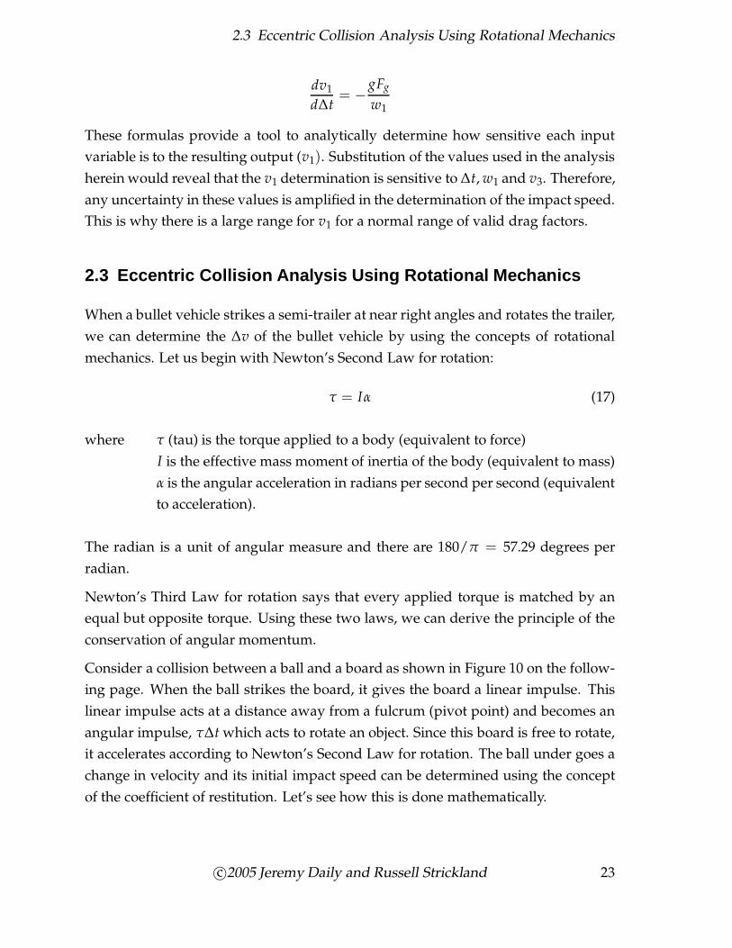
Consider a collision between a ball and a board as shown in Figure 10 on the follow-
ing page. When the ball strikes the board, it gives the board a linear impulse. This
linear impulse acts at a distance away from a fulcrum (pivot point) and becomes an
angular impulse, τ∆t which acts to rotate an object. Since this board is free to rotate,
it accelerates according to Newton’s Second Law for rotation. The ball under goes a
change in velocity and its initial impact speed can be determined using the concept
of the coefficient of restitution. Let’s see how this is done mathematically.
c©2005 Jeremy Daily and Russell Strickland 23
2 Reconstruction of Staged Crashes
bPivot Pointτ = Iα
Fc1
Fc2
h
F = ma
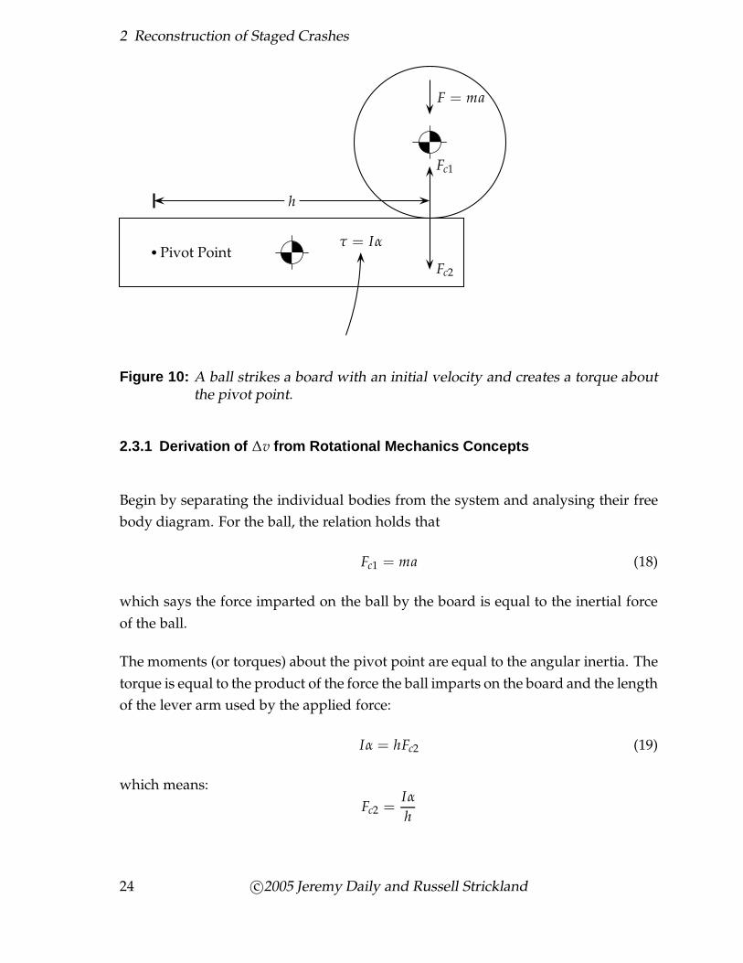
Figure 10: A ball strikes a board with an initial velocity and creates a torque aboutthe pivot point.
2.3.1 Derivation of ∆v from Rotational Mechanics Concepts
Begin by separating the individual bodies from the system and analysing their free
body diagram. For the ball, the relation holds that
Fc1 = ma (18)
which says the force imparted on the ball by the board is equal to the inertial force
of the ball.
The moments (or torques) about the pivot point are equal to the angular inertia. The
torque is equal to the product of the force the ball imparts on the board and the length
of the lever arm used by the applied force:
Iα = hFc2 (19)
which means:
Fc2 =Iα
h
24 c©2005 Jeremy Daily and Russell Strickland
2.3 Eccentric Collision Analysis Using Rotational Mechanics
By Newton’s Third Law:
−Fc1 = Fc2 (20)
Making the substitution of eqs. (18) and (19) into eq. (20) gives:
−ma =Iα
h(21)
Substitute a = ∆v∆t into eq. (21) to get:
−m∆v
∆t=
Iα
h(22)
An analogous substitution can be made for the angular acceleration:
α =∆ω
∆t(23)
where ω (omega) is the angular velocity in radians per second. Continue by substi-
tuting the value for α into eq. (22):
−m∆v
∆t=
I∆ω
h∆t(24)
Multiplying both sides of the equation by h∆t yields:
−mh∆v = I∆ω (25)
The definition of ∆ω is similar to ∆v:
∆ω = ωi − ω f (26)
where ω f is the post impact angular velocity of the board
ωi is the pre impact angular velocity of the board. In this case, wi = 0.
Since the initial angular velocity is zero, we will let ω f = ω so ∆ω = −ω. Continue
by substituting this simplification into eq. (25):
−mh∆v = −Iω
c©2005 Jeremy Daily and Russell Strickland 25
2 Reconstruction of Staged Crashes
Multiply though by −1 to get:
mh∆v = Iω
Now solve for ∆v:
∆v =Iω
mh(27)
This result says we can determine the speed change of the ball if we can determine
the angular velocity of the board after the impact. We will extend this same concept
to vehicle hitting the side of a trailer.
2.3.2 The Work–Energy Theorem for Rotation
The work–energy theorem says that the work done by a torque comes from kinetic
energy:
KE = Work (28)
The kinetic energy of a rotating object is:
KE =1
2Iω2 (29)
The work done by a torque is:
Work = τθ (30)
where τ is the torque and θ (theta) is the rotational displacement in radians. Also the
definition of torque is:
τ = Fh (31)
where F is a force and h is the lever arm for the force. If we substitute eq. (31) into
eq. (30) and invoke eq. (28), then we get:
1
2Iω2 = Fhθ (32)
Solving for ω gives:
ω =
√
2Fhθ
I(33)
26 c©2005 Jeremy Daily and Russell Strickland
2.3 Eccentric Collision Analysis Using Rotational Mechanics
2.3.3 Application to Side Impact Collisions
The evidence of the scene indicates the tractor did not move during the collision. This
means the kingpin can be considered rigid. As a result, the rotation of the trailer oc-
curs around the kingpin and all measurements are referenced to this point as shown
in Figure 6. Recall from Section 2.1.4 the mass moment of inertia of the trailer about
its kingpin is 421,470 ft-lb-sec2. The weight on the rear dual axles is 9550 lbs.
The force used in eq. (33) comes from the friction force of the rear duals (axles 3
and 4). The lever arm for this frictional force is h = 36.4 ft. The tires are sliding
perpendicular to their rolling direction so they are producing the maximum available
force. We can use a lower friction coefficient as an upper value of µL = 0.55 and
µH = 0.65 which give us two distinct values for Fh:
FLh = µLw3,4h
= 0.55(9550)(36.4)
= 191, 191 lb-ft
FHh = µHw3,4h
= 0.65(9550)(36.4)
= 225, 953 lb-ft
All values determined so far are specific to only the trailer.
Nissan Sentra Collision The mass of the Nissan Sentra is computed from the def-
inition of weight:
m =w
g=
2408
32.2= 74.78 slugs
The angle of rotation is determined using the definition of tangent:
θ = tan−1
(rise
run
)
c©2005 Jeremy Daily and Russell Strickland 27
2 Reconstruction of Staged Crashes
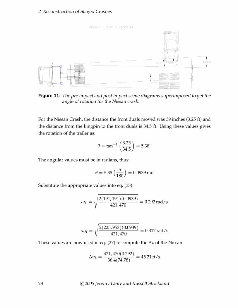
Figure 11: The pre impact and post impact scene diagrams superimposed to get theangle of rotation for the Nissan crash.
For the Nissan Crash, the distance the front duals moved was 39 inches (3.25 ft) and
the distance from the kingpin to the front duals is 34.5 ft. Using these values gives
the rotation of the trailer as:
θ = tan−1
(3.25
34.5
)
= 5.38◦
The angular values must be in radians, thus:
θ = 5.38( π
180
)
= 0.0939 rad
Substitute the appropriate values into eq. (33):
ωL =
√
2(191, 191)(0.0939)
421, 470= 0.292 rad/s
ωH =
√
2(225, 953)(0.0939)
421, 470= 0.317 rad/s
These values are now used in eq. (27) to compute the ∆v of the Nissan:
∆vL =421, 470(0.292)
36.4(74.78)= 45.21 ft/s
28 c©2005 Jeremy Daily and Russell Strickland
2.3 Eccentric Collision Analysis Using Rotational Mechanics
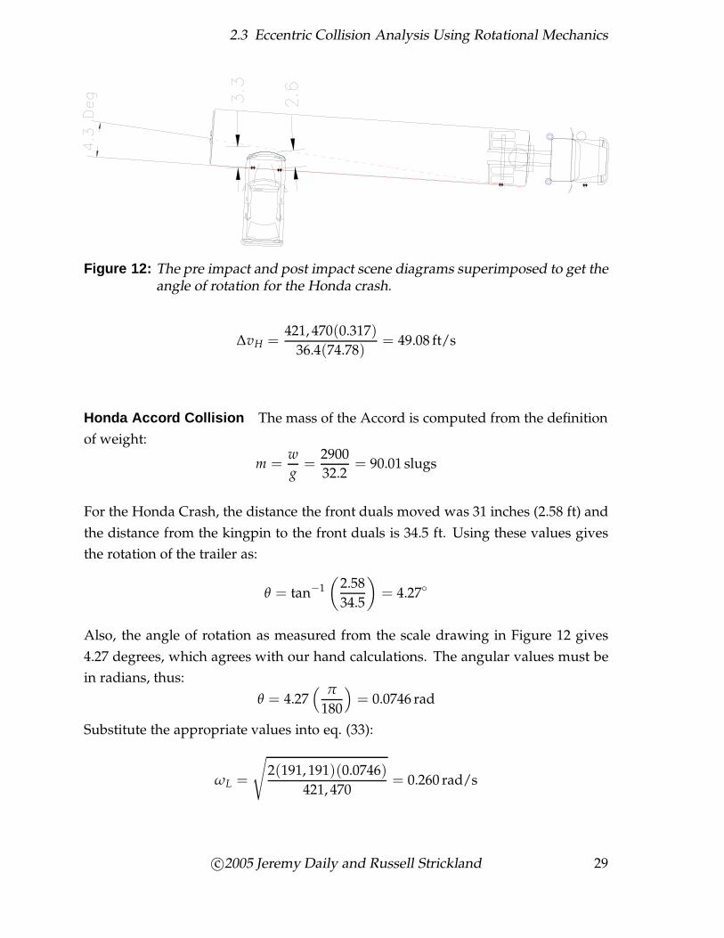
Figure 12: The pre impact and post impact scene diagrams superimposed to get theangle of rotation for the Honda crash.
∆vH =421, 470(0.317)
36.4(74.78)= 49.08 ft/s
Honda Accord Collision The mass of the Accord is computed from the definition
of weight:
m =w
g=
2900
32.2= 90.01 slugs
For the Honda Crash, the distance the front duals moved was 31 inches (2.58 ft) and
the distance from the kingpin to the front duals is 34.5 ft. Using these values gives
the rotation of the trailer as:
θ = tan−1
(2.58
34.5
)
= 4.27◦
Also, the angle of rotation as measured from the scale drawing in Figure 12 gives
4.27 degrees, which agrees with our hand calculations. The angular values must be
in radians, thus:
θ = 4.27( π
180
)
= 0.0746 rad
Substitute the appropriate values into eq. (33):
ωL =
√
2(191, 191)(0.0746)
421, 470= 0.260 rad/s
c©2005 Jeremy Daily and Russell Strickland 29
2 Reconstruction of Staged Crashes
ωH =
√
2(225, 953)(0.0746)
421, 470= 0.283 rad/s
These values are now used in eq. (27) to compute the ∆v of the Honda:
∆vL =421, 470(0.260)
36.4(90.01)= 33.48 ft/s
∆vH =421, 470(0.283)
36.4(90.01)= 36.40 ft/s
2.3.4 Computing Impact Speed from ∆v
In order to compute the impact speed from ∆v we must define the coefficient of
restitution as:
ǫ =v4 − v3
v1 − v2(34)
The coefficient of restitution is the ratio of the relative velocity after the collision to
the relative velocity before the collision. It has a value from 0 to 1. For some low
speed impacts, the coefficient of restitution can be as high as 0.3. As the speeds get
larger, the coefficient of restitution drops. We will assume a value (on the high side)
of 0.1. A higher value for the coefficient of restitution leads to a lower impact speed.
We also have a definition of ∆v that is:
∆v = v1 − v3
or
v3 = v1 − ∆v
Let v2 = 0 and substitute the expression for v3 into eq. (34):
ǫ =v4 − (v1 − ∆v)
v1 − 0
30 c©2005 Jeremy Daily and Russell Strickland
2.3 Eccentric Collision Analysis Using Rotational Mechanics
Solve for v1:
ǫv1 = v4 − v1 + ∆v
v1 + ǫv1 = v4 + ∆v
v1(1 + ǫ) = v4 + ∆v
v1 =v4 + ∆v
1 + ǫ(35)
The value of v4 is determined from the kinematics of rotating bodies:
v4 = rω (36)
where r is the distance between the centroid of the collision and the point of rotation.
The variable of ω describes the post impact angular velocity and is determined using
eq. (33). Substitute eq. (36) into eq. (35) to get:
v1 =rω + ∆v
1 + ǫ(37)
Impact Speed of the Nissan The value for r is the distance between the kingpin
and the center of the rear duals, 36.4 feet. We can see from eq. (37) that any restitution
decreases the impact velocity. Thus to get the high end of the range of impact speeds,
use no restitution and the high values of ω and ∆v:
v1H =36.4(0.317) + 49.08
1 + 0
= 60.61 ft/s
S1H = 41.33 mph
We know that some restitution exists, but not much. Let’s assume ǫ = 0.1. Also, we
will use the low values for ∆v and ω:
c©2005 Jeremy Daily and Russell Strickland 31
3 Crash Data Analysis and Conclusions
v1L =36.4(0.292) + 45.21
1 + 0.1
= 50.76 ft/s
S1L = 34.61 mph
Our reconstructed impact speed range for the Nissan is between 34 and 41 mph.
Impact Speed of the Honda The same impact area and trailer was hit by the
Honda. Again, to get the high end of the range of impact speeds, use no restitu-
tion and the high values of ω and ∆v:
v1H =36.4(0.283) + 36.40
1 + 0
= 46.70 ft/s
S1H = 31.81 mph
We know that some restitution exists, but not much. Let’s assume ǫ = 0.1. Also, we
will use the low values for ∆v and ω:
v1L =36.4(0.260) + 33.48
1 + 0.1
= 39.04 ft/s
S1L = 26.63 mph
Our reconstructed impact speed range for the Honda is between 27 and 32 mph.
3 Crash Data Analysis and Conclusions
Table 4 shows a comparison of the reconstructed speeds with the actual speeds mea-
sured by a RADAR system. The two under-ride collisions reveal problems when
32 c©2005 Jeremy Daily and Russell Strickland

Table 4: Comparison of speed estimates using reconstruction techniques to mea-sured speeds in miles per hour.
Bullet Test Vehicle Lower Bound Upper Bound Actual Impact Speed
Jeep 38 49 37Voyager 30 52 39Nissan 34 41 39Honda 27 32 31
trying to predict impact speeds using momentum concepts when the vehicle mass
ratios are high. Even though inclusion of external impulses is physically more cor-
rect, it tends to make the speed estimates less conservative (higher). Furthermore,
the impulse forces are difficult to determine, especially when little evidence exists.
It is not recommended to use a momentum analysis in court when high mass ratios
exist.
The impact analysis using rotational mechanics concepts proved to be accurate. More-
over, using the middle values of the ranges yielded answers within a couple miles
per hour. The analysis presented herein is valid and the evidence can be easily gath-
ered at the scene, provided the on-scene investigator is trained to look for evidence
under the trailer.
Another assumption we were able to analyze using instrumentation was the dura-
tion of the crash. Some approximate values are shown in Table 5. The time of the
impact in an under-ride collision is about three times larger than a “normal” crash.
This means the average acceleration would be lower for a given ∆v which would
tend to indicate that passengers in the back seat could possibly survive such crashes
(if they wear seat belts). Furthermore, the effect of external forces become more pro-
nounced since ∆t is larger.
Detailed analysis of the high speed video could reveal parameters such as the coeffi-
cient of restitution, the duration of the crash, and the mechanisms of force generation
during a crash. These values would be helpful in further understanding the physics
of crashes.
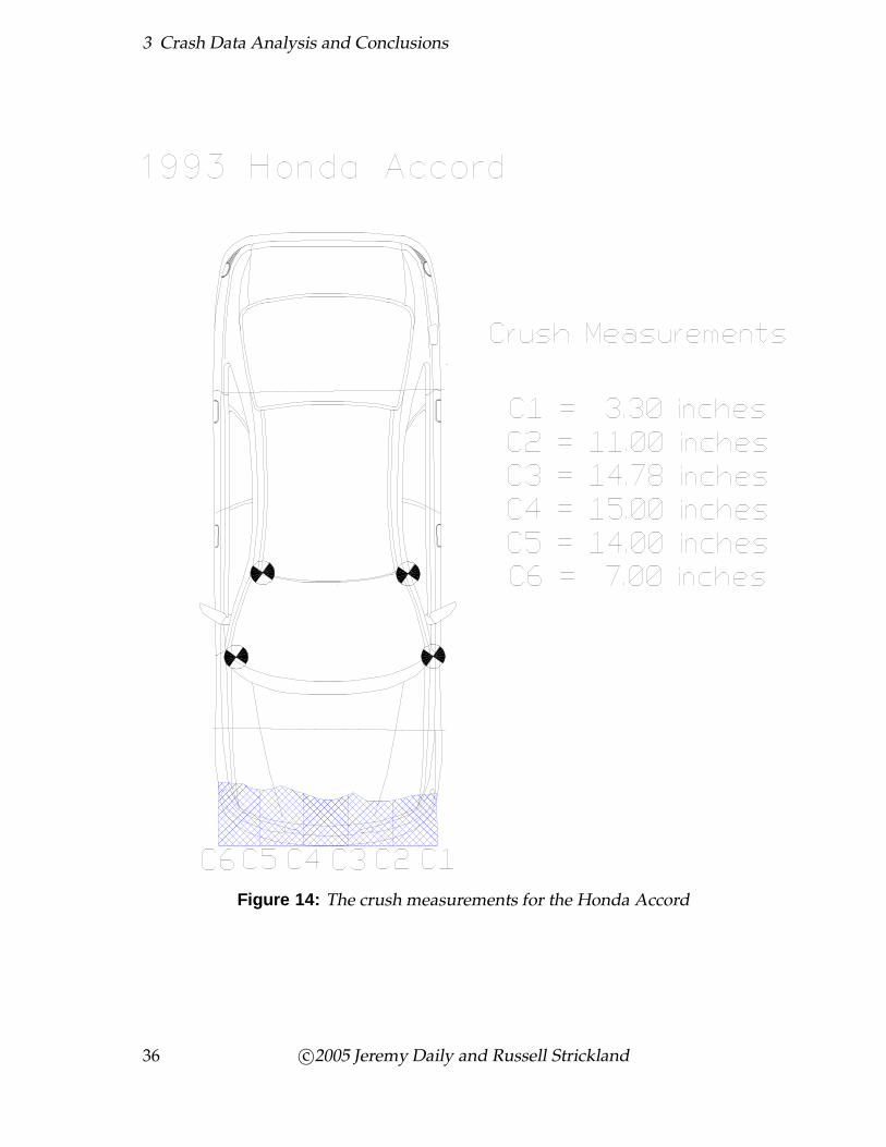
Crush measurements were taken of the cars involved in the side impact crashes.
The analysis of the ∆v using crush is left as an exercise for the reader. The crush
c©2005 Jeremy Daily and Russell Strickland 33
3 Crash Data Analysis and Conclusions
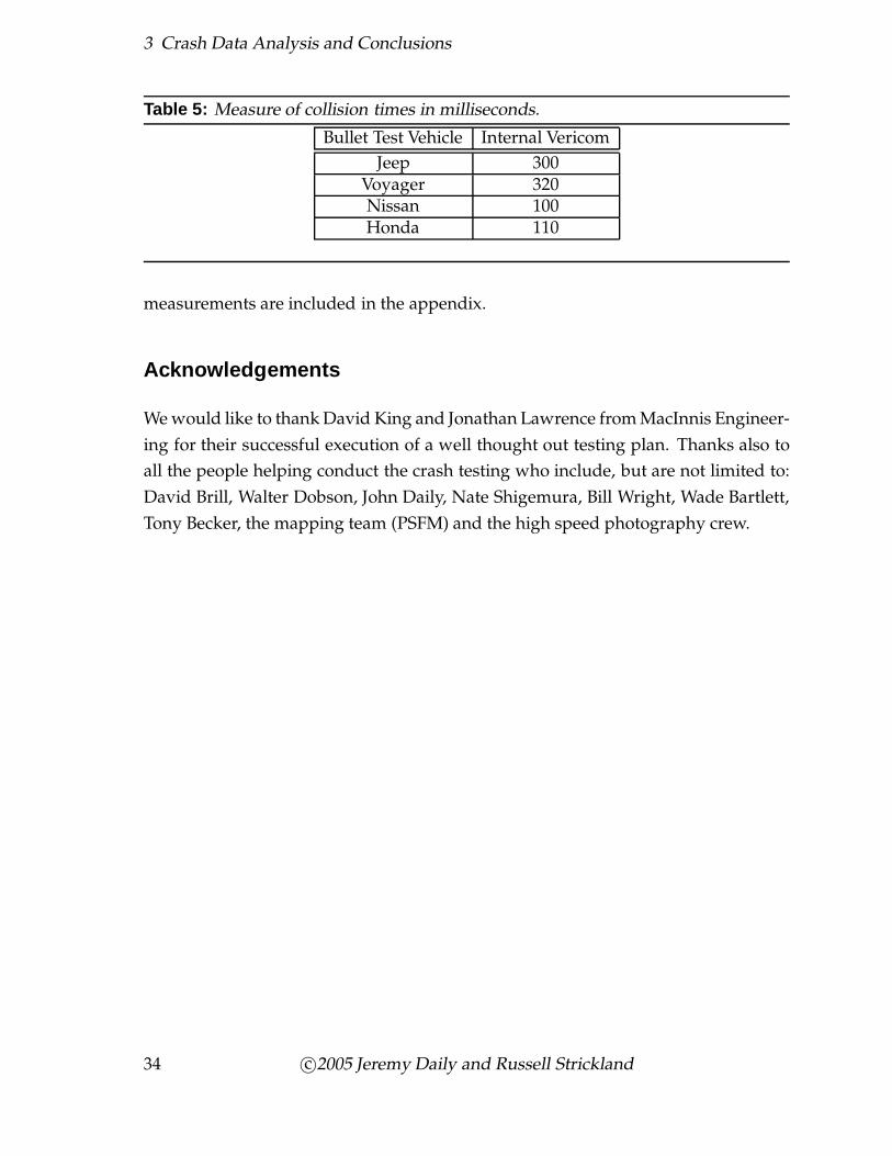
Table 5: Measure of collision times in milliseconds.
Bullet Test Vehicle Internal Vericom
Jeep 300Voyager 320Nissan 100Honda 110
measurements are included in the appendix.
Acknowledgements
We would like to thank David King and Jonathan Lawrence from MacInnis Engineer-
ing for their successful execution of a well thought out testing plan. Thanks also to
all the people helping conduct the crash testing who include, but are not limited to:
David Brill, Walter Dobson, John Daily, Nate Shigemura, Bill Wright, Wade Bartlett,
Tony Becker, the mapping team (PSFM) and the high speed photography crew.
34 c©2005 Jeremy Daily and Russell Strickland
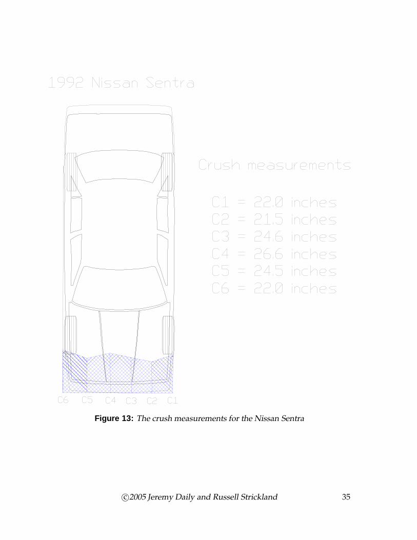
Figure 13: The crush measurements for the Nissan Sentra
c©2005 Jeremy Daily and Russell Strickland 35
3 Crash Data Analysis and Conclusions
Figure 14: The crush measurements for the Honda Accord
36 c©2005 Jeremy Daily and Russell Strickland