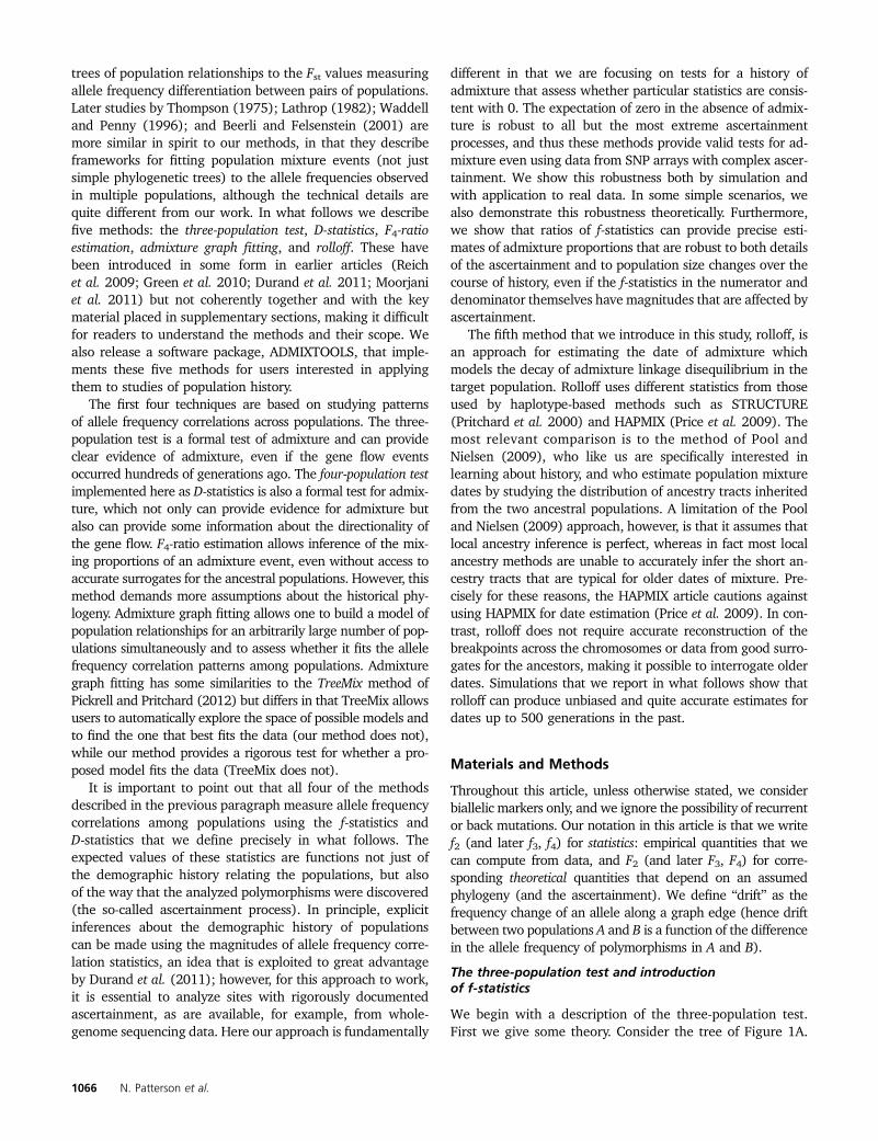
INVESTIGATION

Ancient Admixture in Human HistoryNick Patterson,*,1 Priya Moorjani,† Yontao Luo,‡ Swapan Mallick,† Nadin Rohland,† Yiping Zhan,‡

Teri Genschoreck,‡ Teresa Webster,‡ and David Reich*,†

*Broad Institute of Harvard and Massachusetts Institute of Technology, Cambridge, Massachusetts 02142, †Department ofGenetics, Harvard Medical School, Boston, Massachusetts 02115, and ‡Affymetrix, Inc., Santa Clara, California 95051

ABSTRACT Population mixture is an important process in biology. We present a suite of methods for learning about populationmixtures, implemented in a software package called ADMIXTOOLS, that support formal tests for whether mixture occurred and make itpossible to infer proportions and dates of mixture. We also describe the development of a new single nucleotide polymorphism (SNP)array consisting of 629,433 sites with clearly documented ascertainment that was specifically designed for population genetic analysesand that we genotyped in 934 individuals from 53 diverse populations. To illustrate the methods, we give a number of examples thatprovide new insights about the history of human admixture. The most striking finding is a clear signal of admixture into northernEurope, with one ancestral population related to present-day Basques and Sardinians and the other related to present-day populationsof northeast Asia and the Americas. This likely reflects a history of admixture between Neolithic migrants and the indigenous Mesolithicpopulation of Europe, consistent with recent analyses of ancient bones from Sweden and the sequencing of the genome of theTyrolean “Iceman.”

ADMIXTURE between populations is a fundamental pro-cess that shapes genetic variation and disease risk. For

example, African Americans and Latinos derive their ge-nomes from mixtures of individuals who trace their ancestryto divergent populations. Study of the ancestral origin of theadmixed individuals provides an opportunity to infer thehistory of the ancestral groups, some of whommay no longerbe extant. The two main classes of methods in this fieldare local ancestry-based methods and global ancestry-basedmethods. Local ancestry-based methods such as LAMP(Sankararaman et al. 2008), HAPMIX (Price et al. 2009),and PCADMIX (Brisbin 2010) deconvolve ancestry at eachlocus in the genome and provide individual-level informationabout ancestry. While these methods provide valuable insightsinto the recent history of populations, they have reducedpower to detect older events. The most commonly used meth-ods for studying global ancestry are principal component anal-ysis (PCA) (Patterson et al. 2006) and model-based clusteringmethods such as STRUCTURE (Pritchard et al. 2000) and

ADMIXTURE (Alexander et al. 2009). While these are power-ful tools for detecting population substructure, they do notprovide any formal tests for admixture (the patterns in datadetected using these methods can be generated by multiplepopulation histories). For instance, Novembre et al. (2008)showed that isolation-by-distance can generate PCA gradientsthat are similar to those that arise from long-distance histor-ical migrations, making PCA results difficult to interpret froma historical perspective. STRUCTURE/ADMIXTURE results arealso difficult to interpret historically, because these methodswork either without explicitly fitting a historical model or byfitting a model that assumes that all the populations haveradiated from a single ancestral group, which is unrealistic.

An alternative approach is to make explicit inferencesabout history by fitting phylogenetic tree-based models togenetic data. A limitation of this approach, however, is thatmany of these methods do not allow for the possibility ofmigrations between groups, whereas most human popula-tions derive ancestry from multiple ancestral groups. Indeedthere is only a handful of examples of human groups in whichthere is no evidence of genetic admixture today. In this article,we describe a suite of methods that formally test for a historyof population mixture and allow researchers to build modelsof population relationships (including admixture) that fitgenetic data. These methods are inspired by the ideas byCavalli-Sforza and Edwards (1967), who fit phylogenetic

Copyright © 2012 by the Genetics Society of Americadoi: 10.1534/genetics.112.145037Manuscript received March 24, 2012; accepted for publication August 28, 2012Supporting information is available online at http://www.genetics.org/lookup/suppl/doi:10.1534/genetics.112.145037/-/DC1.1Corresponding author: Broad Institute, 7 Cambridge Center, Cambridge, MA 02142.E-mail: nickp@broadinstitute.org

Genetics, Vol. 192, 1065–1093 November 2012 1065

trees of population relationships to the Fst values measuringallele frequency differentiation between pairs of populations.Later studies by Thompson (1975); Lathrop (1982); Waddelland Penny (1996); and Beerli and Felsenstein (2001) aremore similar in spirit to our methods, in that they describeframeworks for fitting population mixture events (not justsimple phylogenetic trees) to the allele frequencies observedin multiple populations, although the technical details arequite different from our work. In what follows we describefive methods: the three-population test, D-statistics, F4-ratioestimation, admixture graph fitting, and rolloff. These havebeen introduced in some form in earlier articles (Reichet al. 2009; Green et al. 2010; Durand et al. 2011; Moorjaniet al. 2011) but not coherently together and with the keymaterial placed in supplementary sections, making it difficultfor readers to understand the methods and their scope. Wealso release a software package, ADMIXTOOLS, that imple-ments these five methods for users interested in applyingthem to studies of population history.

The first four techniques are based on studying patternsof allele frequency correlations across populations. The three-population test is a formal test of admixture and can provideclear evidence of admixture, even if the gene flow eventsoccurred hundreds of generations ago. The four-population testimplemented here as D-statistics is also a formal test for admix-ture, which not only can provide evidence for admixture butalso can provide some information about the directionality ofthe gene flow. F4-ratio estimation allows inference of the mix-ing proportions of an admixture event, even without access toaccurate surrogates for the ancestral populations. However, thismethod demands more assumptions about the historical phy-logeny. Admixture graph fitting allows one to build a model ofpopulation relationships for an arbitrarily large number of pop-ulations simultaneously and to assess whether it fits the allelefrequency correlation patterns among populations. Admixturegraph fitting has some similarities to the TreeMix method ofPickrell and Pritchard (2012) but differs in that TreeMix allowsusers to automatically explore the space of possible models andto find the one that best fits the data (our method does not),while our method provides a rigorous test for whether a pro-posed model fits the data (TreeMix does not).

It is important to point out that all four of the methodsdescribed in the previous paragraph measure allele frequencycorrelations among populations using the f-statistics andD-statistics that we define precisely in what follows. Theexpected values of these statistics are functions not just ofthe demographic history relating the populations, but alsoof the way that the analyzed polymorphisms were discovered(the so-called ascertainment process). In principle, explicitinferences about the demographic history of populationscan be made using the magnitudes of allele frequency corre-lation statistics, an idea that is exploited to great advantageby Durand et al. (2011); however, for this approach to work,it is essential to analyze sites with rigorously documentedascertainment, as are available, for example, from whole-genome sequencing data. Here our approach is fundamentally

different in that we are focusing on tests for a history ofadmixture that assess whether particular statistics are consis-tent with 0. The expectation of zero in the absence of admix-ture is robust to all but the most extreme ascertainmentprocesses, and thus these methods provide valid tests for ad-mixture even using data from SNP arrays with complex ascer-tainment. We show this robustness both by simulation andwith application to real data. In some simple scenarios, wealso demonstrate this robustness theoretically. Furthermore,we show that ratios of f-statistics can provide precise esti-mates of admixture proportions that are robust to both detailsof the ascertainment and to population size changes over thecourse of history, even if the f-statistics in the numerator anddenominator themselves have magnitudes that are affected byascertainment.

The fifth method that we introduce in this study, rolloff, isan approach for estimating the date of admixture whichmodels the decay of admixture linkage disequilibrium in thetarget population. Rolloff uses different statistics from thoseused by haplotype-based methods such as STRUCTURE(Pritchard et al. 2000) and HAPMIX (Price et al. 2009). Themost relevant comparison is to the method of Pool andNielsen (2009), who like us are specifically interested inlearning about history, and who estimate population mixturedates by studying the distribution of ancestry tracts inheritedfrom the two ancestral populations. A limitation of the Pooland Nielsen (2009) approach, however, is that it assumes thatlocal ancestry inference is perfect, whereas in fact most localancestry methods are unable to accurately infer the short an-cestry tracts that are typical for older dates of mixture. Pre-cisely for these reasons, the HAPMIX article cautions againstusing HAPMIX for date estimation (Price et al. 2009). In con-trast, rolloff does not require accurate reconstruction of thebreakpoints across the chromosomes or data from good surro-gates for the ancestors, making it possible to interrogate olderdates. Simulations that we report in what follows show thatrolloff can produce unbiased and quite accurate estimates fordates up to 500 generations in the past.

Materials and Methods

Throughout this article, unless otherwise stated, we considerbiallelic markers only, and we ignore the possibility of recurrentor back mutations. Our notation in this article is that we writef2 (and later f3, f4) for statistics: empirical quantities that wecan compute from data, and F2 (and later F3, F4) for corre-sponding theoretical quantities that depend on an assumedphylogeny (and the ascertainment). We define “drift” as thefrequency change of an allele along a graph edge (hence driftbetween two populations A and B is a function of the differencein the allele frequency of polymorphisms in A and B).

The three-population test and introductionof f-statistics

We begin with a description of the three-population test.First we give some theory. Consider the tree of Figure 1A.

1066 N. Patterson et al.

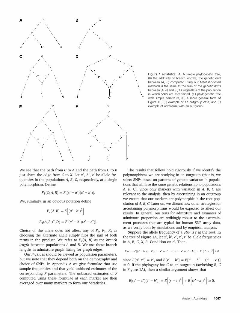
We see that the path from C to A and the path from C to Bjust share the edge from C to X. Let a9, b9, c9 be allele fre-quencies in the populations A, B, C, respectively, at a singlepolymorphism. Define

F3ðC;A;BÞ ¼ E½ðc92 a9Þðc92 b9Þ�:

We, similarly, in an obvious notation define

F2ðA;BÞ ¼ Ehða92b9Þ2

i

F4ðA;B;C;DÞ ¼ E½ða92 b9Þðc92 d9Þ�:

Choice of the allele does not affect any of F2, F3, F4 aschoosing the alternate allele simply flips the sign of bothterms in the product. We refer to F2(A, B) as the branchlength between populations A and B. We use these branchlengths in admixture graph fitting for graph edges.

Our F-values should be viewed as population parameters,but we note that they depend both on the demography andchoice of SNPs. In Appendix A we give formulae that usesample frequencies and that yield unbiased estimates of thecorresponding F parameters. The unbiased estimates of Fcomputed using these formulae at each marker are thenaveraged over many markers to form our f-statistics.

The results that follow hold rigorously if we identify thepolymorphisms we are studying in an outgroup (that is, weselect SNPs based on patterns of genetic variation in popula-tions that all have the same genetic relationship to populationsA, B, C). Since only markers with variation in A, B, C arerelevant to the analysis, then by ascertaining in an outgroupwe ensure that our markers are polymorphic in the root pop-ulation of A, B, C. Later on, we discuss how other strategies forascertaining polymorphisms would be expected to affect ourresults. In general, our tests for admixture and estimates ofadmixture proportion are strikingly robust to the ascertain-ment processes that are typical for human SNP array data,as we verify both by simulations and by empirical analysis.

Suppose the allele frequency of a SNP is r at the root. Inthe tree of Figure 1A, let a9, b9, c9, x9, r9 be allele frequenciesin A, B, C, X, R. Condition on r9. Then

E½ðc92 a9Þðc92 b9Þ� ¼ E½ðc92 x9þ x92 a9Þðc92 x9þ x92 b9Þ� ¼ Ehðc92x9Þ2

i$ 0

since E[a9|x9] = x9, and E[x9 2 b9] = E[r9 2 b9 2 (r9 2 x9)]= 0. If the phylogeny has C as an outgroup (switching B, Cin Figure 1A), then a similar argument shows that

E½ðc92 a9Þðc92 b9Þ� ¼ Ehðr92c9Þ2

iþ E

hðr92x9Þ2

i$ 0:

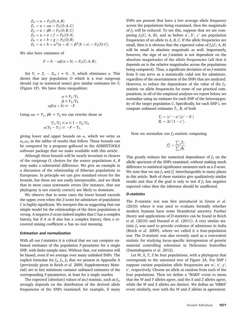
Figure 1 f-statistics: (A) A simple phylogenetic tree,(B) the additivity of branch lengths; the genetic driftbetween (A, B) computed using our f-statistic-basedmethods is the same as the sum of the genetic driftsbetween (A, B) and (B, C), regardless of the populationin which SNPs are ascertained, (C) phylogenetic treewith simple admixture, (D) a more general form ofFigure 1C, (E) example of an outgroup case, and (F)example of admixture with an outgroup.

Ancient Admixture 1067

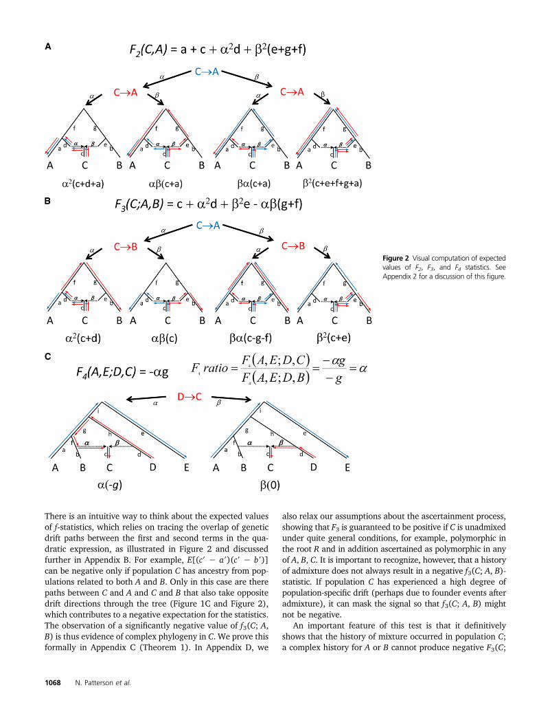
There is an intuitive way to think about the expected valuesof f-statistics, which relies on tracing the overlap of geneticdrift paths between the first and second terms in the qua-dratic expression, as illustrated in Figure 2 and discussedfurther in Appendix B. For example, E[(c9 2 a9)(c9 2 b9)]can be negative only if population C has ancestry from pop-ulations related to both A and B. Only in this case are therepaths between C and A and C and B that also take oppositedrift directions through the tree (Figure 1C and Figure 2),which contributes to a negative expectation for the statistics.The observation of a significantly negative value of f3(C; A,B) is thus evidence of complex phylogeny in C. We prove thisformally in Appendix C (Theorem 1). In Appendix D, we

also relax our assumptions about the ascertainment process,showing that F3 is guaranteed to be positive if C is unadmixedunder quite general conditions, for example, polymorphic inthe root R and in addition ascertained as polymorphic in anyof A, B, C. It is important to recognize, however, that a historyof admixture does not always result in a negative f3(C; A, B)-statistic. If population C has experienced a high degree ofpopulation-specific drift (perhaps due to founder events afteradmixture), it can mask the signal so that f3(C; A, B) mightnot be negative.

An important feature of this test is that it definitivelyshows that the history of mixture occurred in population C;a complex history for A or B cannot produce negative F3(C;

Figure 2 Visual computation of expectedvalues of F2, F3, and F4 statistics. SeeAppendix 2 for a discussion of this figure.

1068 N. Patterson et al.

A, B). To explain why this is so, we recapitulate materialfrom Reich et al. (2009). If population A is admixed then if wepick an allele of A, it must have originated in one of the admix-ing populations. Pick alleles a, b from populations A and B andg1, g2 independently from C, coding 1 for a reference allele,0 for a variant, etc. Thus, F3(C; A, B) = E[(g1 2 a)](g2 2 b)].Suppose population A is admixed; B and C are not admixed.The allele a sampled from population A can take more thanone path through the ancestral populations. F3(C; A, B) canthen be computed as a weighted average over the possiblephylogenies, in all of which the quantity has a positive expec-tation because A and B are now unadmixed (Appendix B andFigure 2). In conclusion, the diagram makes it visually evidentthat if F3(C; A, B) , 0 then population C itself must havea complex history.

Additivity of F2 along a tree branch

In this article we consider generalizations of phylogenetictrees where graph edges indicate that one population isa descendant of another. Consider the phylogenetic tree inFigure 1B, and a marker polymorphic at the root. Drift ona given edge is a random variable with mean 0. For if A / Bis a graph edge, with corresponding allele frequencies a9, b9,

E½b9ja9� ¼ a9:

This is the martingale property of allele frequency diffusion.Drifts on two distinct edges of a tree are orthogonal, whereorthogonality of random variables X, Y simply means thatE[XY] = 0. In our context this means that the drifts ondistinct edges have mean 0 and are uncorrelated.

A valuable feature of our F-statistics definition is thatbranch lengths on the tree (as defined by F2) are additive.We illustrate this with an example from human history (Fig-ure 1B). (We note that all examples in this article refer tohuman history, although the methods should apply equallywell to other species.) In this example, A, and C are present-day populations that split from an ancestral population X. Bis an ancestral population to C. For instance, A might bemodern Yoruba, C a European population, and B an ancientpopulation, perhaps a sample from archeological material ofa population that existed thousands of years ago. We as-sume here that we ascertain in an outgroup (implying poly-morphism at the root) and again assume neutrality and thatwe can ignore recurrent or backmutations. Then we meanby additivity that

F2ðA;CÞ ¼ F2ðA;BÞ þ F2ðB;CÞ

for

Ehða92c9Þ2

i¼ E

hða92b9þ b92c9Þ2

i

¼ Ehða92b9Þ2

iþ E

hðb92c9Þ2

iþ 2E½ða92 b9Þðb92 c9Þ�;

but the last term is 0 since the change in allele frequencies(drifts) X / A, X / B, B / C are all uncorrelated.

We remark that our F2-distance resembles the familiarFst, but is not the same. In particular, parts of a graph thatare far from the root (in genetic drift distance) have F2 re-duced. Some insight into this effect is given by consideringthe simple graph

R/t1 A/

t2 B;

where t1, t2 are drift times on the standard diffusion time-scale (two random alleles of B have probability e2t2 thatthey have not coalesced in the ancestral population A).

If r9, a9, b9 are allele frequencies in R, A, B, respectively,then F2(A, B) = E[(a9 2 b9)2]. Write Er9, Ea9 for expectationsconditional on population allele frequencies r9, a9. ThenEa9½ða92b9Þ2� ¼ a9ð12 a9Þð12 e2t2Þ (Nei 1987, Chap. 13).Moreover Er9½a9ð12 a9Þ� ¼ r9ð12 r9Þe2t1. Hence

F2ðA;BÞ ¼ E½r9ð12 r9Þe2t1ð12 e2t2Þ�:

Informally the drift from R / A shrinks F2(A, B) by a factore2t1 . Thus expected drift is additive,

F2ðR;BÞ ¼ F2ðR;AÞ þ F2ðA;BÞ;

but the drift does depend on ascertainment. For a given edge,the more distant the root, the smaller the drift. A looseanalogy is projecting a curved surface, such as part of theglobe, into a plane. Locally all is well, but any projection willcause distortion in the large. Additivity in F2 distances is all werequire in what follows. We note that there is no assumptionhere that population sizes are constant along a branch edge,and so we are not assuming linearity of branch lengths in time.

Expected values of our f-statistics

We can calculate expected values for our f-statistics, at leastfor simple demographic histories that involve populationsplits and admixture events. We assume that genetic driftevents on distinct edges are uncorrelated, which as men-tioned before will be true if we ascertain in an outgroup,and our alleles are neutral.

We give an illustration for f3-statistics. Consider the de-mography shown in Figure 1C. Populations E, F split froma root population R. G then was formed by admixture inproportions a: b (b = 1 2 a). Modern populations A, B, Care then formed by drift from E, F, G. We want to calculate theexpected value of f3(C; A, B). Assume that our ascertainmentis such that drifts on distinct edges are orthogonal, which willhold true if we ascertained the markers in an outgroup.

We recapitulate some material from (Reich et al. 2009,Supplementary S2, Sect. 2.2). As before let a9, b9, c9 bepopulation allele frequencies in A, B, C, and let g9 be theallele frequency in G and so on:

F3ðC;A;BÞ ¼ E½ðc92 a9Þðc92 b9Þ�:

We see by orthogonality of drifts that

F3ðC;A;BÞ ¼ E½ðg92 a9Þðg92 b9Þ� þ Ehðg92c9Þ2

i;

Ancient Admixture 1069

which we write as

F3ðC;A;BÞ ¼ F3ðG;A;BÞ þ F2ðC;GÞ: (1)

Now, label alleles at a marker 0, 1. Then picking chromo-somes from our populations independently we can write

F3ðG;A;BÞ ¼ E½ðg12 a1Þðg22 b1Þ�;

where a1, b1 are alleles chosen randomly in populations A, Band g1, g2 are alleles chosen randomly and independently inpopulation G. Similarly, we define e1, e2, f1, and f2. However,g1 originated from E with probability a and so on. Thus

F3ðG;A;BÞ ¼ E½ðg1 2 a1Þðg2 2 b1Þ�¼ a2E½ðe1 2 a1Þðe22 b1Þ�

þ b2E½ðf1 2 a1Þðf2 2 b1Þ�þ abE½ðe1 2 a1Þðf12 b1Þ�þ abE½ðf12 a1Þðe1 2 b1Þ�;

where a1, a2 are independently picked from E and b1, b2from F. The first three terms vanish. Further

E½ðf1 2 a1Þðe1 2 b1Þ� ¼ 2 Ehðe12f1Þ2

i:

This shows that under our assumptions of orthogonal drifton distinct edges,

F3ðC;A;BÞ ¼ F2ðC;GÞ2abF2ðE; FÞ: (2)

It might appear that Figure 1C is too restricted, as it assumesthat the admixing populations E, F are ancestral to A, B andthat we should consider the more general graph shown inFigure 1D. But it turns out that using our f-statistics alone(and not the more general allelic spectrum) that even if a, bare known, we can obtain information only about

a2uþ b2y þ w:

Thus in fitting admixture graphs to f-statistics, we can, with-out loss of generality, fit all the genetic drift specific to theadmixed population on the lineage directly ancestral to theadmixed population (the lineage leading from C to G inFigure 1C).

The outgroup case

Care though is needed in interpretation. Consider Figure 1E.Here a similar calculation to the one just given shows (againassuming orthogonality of drift on each edge) that

F3ðC;A; YÞ ¼ F2ðC;GÞ þ b2F2ðF; XÞ2abF2ðE; XÞ: (3)

Note that Y has little to do with the admixture into C and weobtain the same F3 value for any population Y that splits offfrom A more anciently than X.

We call this case, where we have apparent admixturebetween A and Y, the outgroup case, and it needs to be care-fully considered when recovering population relationships.

Estimates of mixing proportions

We want to estimate, or at least bound, the mixing pro-portions that have resulted in the ancestral population of C.With further strong assumptions on the phylogeny wecan get quite precise estimates even without accurate surro-gates for the ancestral populations (see Reich et al. 2009 andthe F4-ratio estimation that we describe below, for examples).Also if we have data from populations that are accurate sur-rogates for the ancestral admixing population (and we canignore the drift post admixture), the problem is much easier.For instance, in Patterson et al. (2010) we give an estimatorthat works well even when the sample sizes of the relevantpopulations are small, and we have multiple admixing pop-ulations whose deep phylogenetic relationships we may notunderstand. Here we show a method that obtains usefulbounds, without requiring full knowledge of the phylogeny,although the bounds are not very precise. Note that althoughour three-population test remains valid even if the popula-tions A, B are admixed, the mixing proportions we calculateare not meaningful unless the assumed phylogeny is at leastroughly correct. Indeed even discussing mixing from an an-cestral population of A hardly makes sense if A is admixeditself subsequent to the admixing event in C. This is discussedfurther when we present data from Human Genome DiversityPanel (HGDP) populations.

In much of the work in this article, we analyze somepopulations A, B, C and need an outgroup, which split offfrom the ancestral population of A, B, C before the popu-lation split of A, B. For example, in Figure 1E, Y is such anoutgroup. Usually, when studying a group of populationswithin a species, a plausible outgroup can be proposed.The outgroup assumption can then be checked using themethods of this article, by adding an individual froma more distantly related population, which can be treatedas a second outgroup. For instance, with human popu-lations from Eurasia, Yoruba or San Bushmen from sub-Saharan Africa will often be plausible outgroups.1 Oursecond outgroup here is simply being used to check a phy-logenetic assumption in our primary analysis, and we donot require polymorphism at the root for this narrow pur-pose. Chimpanzee is always a good second outgroup forstudies of humans.

Consider the phylogeny of Figure 1F. Here a, b aremixing parameters (a + b = 1) and we show drift dis-tances along the graph edges. Note that here we use a,b,. . ., as branch lengths (F2 distances), not sample or pop-ulation allele frequencies as we do elsewhere in this arti-cle. Thus, for example, F2(O, X) = u. Now we can obtainestimates of

1 There is no completely satisfactory term for the ‘Khoisan’ peoples of southern Africa;see Barnard (1992, introduction) for a sensitive discussion. We prefer ‘Bushmen’following Barnard. However, the standard name for the HGDP Bushmen sample is‘San’ in the genetic literature [for example Cann et al. (2002)], and we use thisspecifically to refer to these samples.

1070 N. Patterson et al.

Z0 ¼ u ¼ F3ðO;A;BÞZ1 ¼ uþ aa ¼ F3ðO;A;CÞZ2 ¼ uþ bb ¼ F3ðO;B;CÞZ3 ¼ uþ aþ f ¼ F2ðO;AÞZ4 ¼ uþ bþ g ¼ F2ðO;BÞZ5 ¼ uþ hþ a2ðaþ dÞ þ b2ðbþ eÞ ¼ F2ðO;CÞ:

We also have estimates of

F ¼ h2abðaþ bÞ ¼ F3ðC;A;BÞ:

Set Yi = Zi 2 Z0, i = 0. . .5, which eliminates u. Thisshows that any population O which is a true outgroupshould (up to statistical noise) give similar estimates for Yi(Figure 1F). We have three inequalities:

a$ Y1=Y3b$ Y2=Y4

abðaþ bÞ# 2F:

Using aa = Y1, bb = Y2 we can rewrite these as

Y1=Y3#a#12 Y2=Y4aðY2 2 Y1Þ$ 2F2 Y1;

giving lower and upper bounds on a, which we write asaL,aU in the tables of results that follow. These bounds canbe computed by a program qpBound in the ADMIXTOOLSsoftware package that we make available with this article.

Although these bounds will be nearly invariant to choicesof the outgroup O, choices for the source populations A, Bmay make a substantial difference. We give an example ina discussion of the relationship of Siberian populations toEuropeans. In principle we can give standard errors for thebounds, but these are not easily interpretable, and we thinkthat in most cases systematic errors (for instance, that ourphylogeny is not exactly correct) are likely to dominate.

We observe that in some cases the lower bound exceedsthe upper, even when the Z-score for admixture of populationC is highly significant. We interpret this as suggesting that oursimple model for the relationships of the three populations iswrong. A negative Z-score indeed implies that C has a complexhistory, but if A or B also has a complex history, then a re-covered mixing coefficient a has no real meaning.

Estimation and normalization

With all our f-statistics it is critical that we can compute un-biased estimates of the population F-parameter for a singleSNP, with finite sample sizes. Without that, our estimates willbe biased, even if we average over many unlinked SNPs. Theexplicit formulae for f2, f3, f4 that we present in Appendix A(previously given in Reich et al. 2009, Supplementary Mate-rial) are in fact minimum variance unbiased estimates of thecorresponding F-parameters, at least for a single marker.

The expected (absolute) values of an f-statistic, such as f3,strongly depends on the distribution of the derived allelefrequencies of the SNPs examined; for example, if many

SNPs are present that have a low average allele frequencyacross the populations being examined, then the magnitudeof f3 will be reduced. To see this, suppose that we are com-puting f3(C; A, B), and as before a9, b9, c9 are populationfrequencies of an allele in A, B, C. If the allele frequencies aresmall, then it is obvious that the expected value of f3(C; A, B)will be small in absolute magnitude as well. Importantly,however, the sign of an f-statistic is not dependent on theabsolute magnitudes of the allele frequencies (all that itdepends on is the relative magnitudes across the populationsbeing compared). Thus, a significant deviation of an f-statisticfrom 0 can serve as a statistically valid test for admixture,regardless of the ascertainment of the SNPs that are analyzed.However, to reduce the dependence of the value of the f3-statistic on allele frequencies for some of our practical com-putations, in all of the empirical analyses we report below, wenormalize using an estimate for each SNP of the heterozygos-ity of the target population C. Specifically, for each SNP i, wecompute unbiased estimates Ti, Bi of both

Ti ¼ ðc92 a9Þðc92 b9ÞBi ¼ 2c9ð12 c9Þ:

Now we normalize our f3-statistic computing

f⋆3 ¼P

iTiPiBi

:

This greatly reduces the numerical dependence of f3 on theallelic spectrum of the SNPs examined, without making muchdifference to statistical significance measures such as a Z-score.We note that we use f3 and f ⋆3 interchangeably in many placesin this article. Both of these statistics give qualitatively similarresults and thus if the goal is only to test if f3 has negativeexpected value then the inference should be unaffected.

D-statistics

The D-statistic test was first introduced in Green et al.(2010) where it was used to evaluate formally whethermodern humans have some Neandertal ancestry. Furthertheory and applications of D-statistics can be found in Reichet al. (2010) and Durand et al. (2011). A very similar sta-tistic f4 was used to provide evidence of admixture in India(Reich et al. 2009), where we called it a four-populationtest. The D-statistic was also recently used as a convenientstatistic for studying locus-specific introgression of geneticmaterial controlling coloration in Heliconius butterflies(Dasmahapatra et al. 2012).

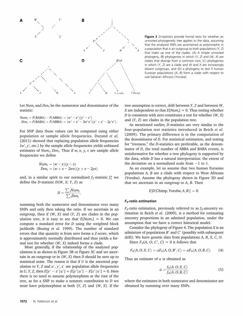
Let W, X, Y, Z be four populations, with a phylogeny thatcorresponds to the unrooted tree of Figure 3A. For SNP isuppose variant population allele frequencies are w9, x9, y9,z9, respectively. Choose an allele at random from each of thefour populations. Then we define a “BABA” event to meanthat the W and Y alleles agree, and the X and Z alleles agree,while the W and X alleles are distinct. We define an “ABBA”event similarly, now with the W and Z alleles in agreement.

Ancient Admixture 1071

Let Numi and Deni be the numerator and denominator of thestatistic:

Numi ¼ PðBABAÞ2 PðABBAÞ ¼ ðw92 x9Þðy92 z9ÞDeni ¼ PðBABAÞ þ PðABBAÞ ¼ ðw9þ x922w9x9Þðy9þ z92 2y9z9Þ:

For SNP data these values can be computed using eitherpopulation or sample allele frequencies. Durand et al.(2011) showed that replacing population allele frequencies(w9, y9, etc.) by the sample allele frequencies yields unbiasedestimates of Numi, Deni. Thus if w, x, y, z are sample allelefrequencies we define

Numi ¼ ðw2 xÞðy2 zÞDeni ¼ ðwþ x2 2wxÞðy þ z2 2yzÞ

and, in a similar spirit to our normalized f3-statistic f ⋆3 wedefine the D-statistic D(W, X; Y, Z) as

D ¼P

iNumiPiDeni

;

summing both the numerator and denominator over manySNPs and only then taking the ratio. If we ascertain in anoutgroup, then if (W, X) and (Y, Z) are clades in the pop-ulation tree, it is easy to see that E[Numi] = 0. We cancompute a standard error for D using the weighted blockjackknife (Busing et al. 1999). The number of standarderrors that this quantity is from zero forms a Z-score, whichis approximately normally distributed and thus yields a for-mal test for whether (W, X) indeed forms a clade.

More generally, if the relationship of the analyzed pop-ulations is as shown in Figure 3B or Figure 3C and we ascer-tain in an outgroup or in {W, X} then D should be zero up tostatistical noise. The reason is that if U is the ancestral pop-ulation to Y, Z and u9, y9, z9 are population allele frequenciesin U, Y, Z, then E[y9 2 z9|u9] = E[y9|u9]2 E[z9|u9] = 0. Herethere is no need to assume polymorphism at the root of thetree, as for a SNP to make a nonzero contribution to D wemust have polymorphism at both {Y, Z} and {W, X}. If the

tree assumption is correct, drift between Y, Z and betweenW,X are independent so that E[Numi] = 0. Thus testing whetherD is consistent with zero constitutes a test for whether (W, X)and (Y, Z) are clades in the population tree.

As mentioned earlier, D-statistics are very similar to thefour-population test statistics introduced in Reich et al.(2009). The primary difference is in the computation ofthe denominator of D. For statistical estimation, and testingfor “treeness,” the D-statistics are preferable, as the denom-inator of D, the total number of ABBA and BABA events, isuninformative for whether a tree phylogeny is supported bythe data, while D has a natural interpretation: the extent ofthe deviation on a normalized scale from 21 to 1.

As an example, let us assume that two human Eurasianpopulations A, B are a clade with respect to West Africans(Yoruba). Assume the phylogeny shown in Figure 3D andthat we ascertain in an outgroup to A, B. Then

E½DðChimp;Yoruba;A;BÞ� ¼ 0:

F4-ratio estimation

F4-ratio estimation, previously referred to as f4-ancestry es-timation in Reich et al. (2009), is a method for estimatingancestry proportions in an admixed population, under theassumption that we have a correct historical model.

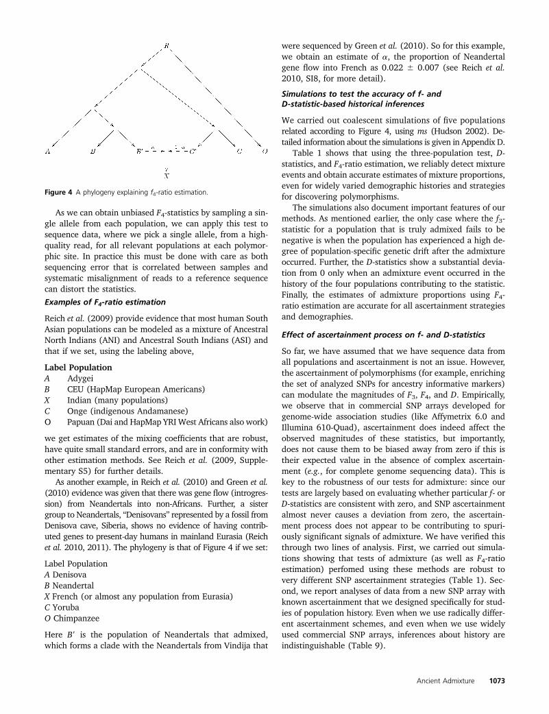
Consider the phylogeny of Figure 4. The population X is anadmixture of populations B9 and C9 (possibly with subsequentdrift). We have genetic data from populations A, B, X, C, O.

Since F4(A, O; C9, C) = 0 it follows that

F4ðA;O;X;CÞ ¼ aF4ðA;O;B9;CÞ ¼ aF4ðA;O;B;CÞ: (4)

Thus an estimate of a is obtained as

a ¼ f4ðA;O;X;CÞf4ðA;O;B;CÞ; (5)

where the estimates in both numerator and denominator areobtained by summing over many SNPs.

Figure 3 D-statistics provide formal tests for whether anunrooted phylogenetic tree applies to the data, assumingthat the analyzed SNPs are ascertained as polymorphic ina population that is an outgroup to both populations (Y, Z)that make up one of the clades. (A) A simple unrootedphylogeny, (B) phylogenies in which (Y, Z) and (W, X) areclades that diverge from a common root, (C) phylogeniesin which (Y, Z) are a clade and W and X are increasinglydistant outgroups, and (D) a phylogeny to test if humanEurasian populations (A, B) form a clade with respect tosub-Saharan Africans (Yoruba).

1072 N. Patterson et al.

As we can obtain unbiased F4-statistics by sampling a sin-gle allele from each population, we can apply this test tosequence data, where we pick a single allele, from a high-quality read, for all relevant populations at each polymor-phic site. In practice this must be done with care as bothsequencing error that is correlated between samples andsystematic misalignment of reads to a reference sequencecan distort the statistics.

Examples of F4-ratio estimation

Reich et al. (2009) provide evidence that most human SouthAsian populations can be modeled as a mixture of AncestralNorth Indians (ANI) and Ancestral South Indians (ASI) andthat if we set, using the labeling above,

Label PopulationA AdygeiB CEU (HapMap European Americans)X Indian (many populations)C Onge (indigenous Andamanese)O Papuan (Dai and HapMap YRI West Africans also work)

we get estimates of the mixing coefficients that are robust,have quite small standard errors, and are in conformity withother estimation methods. See Reich et al. (2009, Supple-mentary S5) for further details.

As another example, in Reich et al. (2010) and Green et al.(2010) evidence was given that there was gene flow (introgres-sion) from Neandertals into non-Africans. Further, a sistergroup to Neandertals, “Denisovans” represented by a fossil fromDenisova cave, Siberia, shows no evidence of having contrib-uted genes to present-day humans in mainland Eurasia (Reichet al. 2010, 2011). The phylogeny is that of Figure 4 if we set:

Label PopulationA DenisovaB NeandertalX French (or almost any population from Eurasia)C YorubaO Chimpanzee

Here B9 is the population of Neandertals that admixed,which forms a clade with the Neandertals from Vindija that

were sequenced by Green et al. (2010). So for this example,we obtain an estimate of a, the proportion of Neandertalgene flow into French as 0.022 6 0.007 (see Reich et al.2010, SI8, for more detail).

Simulations to test the accuracy of f- andD-statistic-based historical inferences

We carried out coalescent simulations of five populationsrelated according to Figure 4, using ms (Hudson 2002). De-tailed information about the simulations is given in Appendix D.

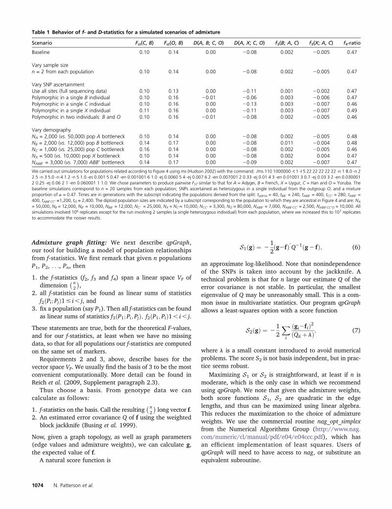
Table 1 shows that using the three-population test, D-statistics, and F4-ratio estimation, we reliably detect mixtureevents and obtain accurate estimates of mixture proportions,even for widely varied demographic histories and strategiesfor discovering polymorphisms.

The simulations also document important features of ourmethods. As mentioned earlier, the only case where the f3-statistic for a population that is truly admixed fails to benegative is when the population has experienced a high de-gree of population-specific genetic drift after the admixtureoccurred. Further, the D-statistics show a substantial devia-tion from 0 only when an admixture event occurred in thehistory of the four populations contributing to the statistic.Finally, the estimates of admixture proportions using F4-ratio estimation are accurate for all ascertainment strategiesand demographies.

Effect of ascertainment process on f- and D-statistics

So far, we have assumed that we have sequence data fromall populations and ascertainment is not an issue. However,the ascertainment of polymorphisms (for example, enrichingthe set of analyzed SNPs for ancestry informative markers)can modulate the magnitudes of F3, F4, and D. Empirically,we observe that in commercial SNP arrays developed forgenome-wide association studies (like Affymetrix 6.0 andIllumina 610-Quad), ascertainment does indeed affect theobserved magnitudes of these statistics, but importantly,does not cause them to be biased away from zero if this istheir expected value in the absence of complex ascertain-ment (e.g., for complete genome sequencing data). This iskey to the robustness of our tests for admixture: since ourtests are largely based on evaluating whether particular f- orD-statistics are consistent with zero, and SNP ascertainmentalmost never causes a deviation from zero, the ascertain-ment process does not appear to be contributing to spuri-ously significant signals of admixture. We have verified thisthrough two lines of analysis. First, we carried out simula-tions showing that tests of admixture (as well as F4-ratioestimation) perfomed using these methods are robust tovery different SNP ascertainment strategies (Table 1). Sec-ond, we report analyses of data from a new SNP array withknown ascertainment that we designed specifically for stud-ies of population history. Even when we use radically differ-ent ascertainment schemes, and even when we use widelyused commercial SNP arrays, inferences about history areindistinguishable (Table 9).

Figure 4 A phylogeny explaining f4-ratio estimation.

Ancient Admixture 1073

Admixture graph fitting: We next describe qpGraph,our tool for building a model of population relationshipsfrom f-statistics. We first remark that given n populationsP1, P2, . . ., Pn, then

1. the f-statistics (f2, f3 and f4) span a linear space VF ofdimension

� n2

�,

2. all f-statistics can be found as linear sums of statisticsf2ðPi; PjÞ1# i, j, and

3. fix a population (say P1). Then all f-statistics can be foundas linear sums of statistics f3ðP1; Pi; PjÞ; f2ðP1; PiÞ1, i, j.

These statements are true, both for the theoretical F-values,and for our f-statistics, at least when we have no missingdata, so that for all populations our f-statistics are computedon the same set of markers.

Requirements 2 and 3, above, describe bases for thevector space VF. We usually find the basis of 3 to be the mostconvenient computationally. More detail can be found inReich et al. (2009, Supplement paragraph 2.3).

Thus choose a basis. From genotype data we cancalculate as follows:

1. f-statistics on the basis. Call the resulting� n2

�long vector f.

2. An estimated error covariance Q of f using the weightedblock jackknife (Busing et al. 1999).

Now, given a graph topology, as well as graph parameters(edge values and admixture weights), we can calculate g,the expected value of f.

A natural score function is

S1ðgÞ ¼ 212ðg2fÞ9Q21ðg2 fÞ; (6)

an approximate log-likelihood. Note that nonindependenceof the SNPs is taken into account by the jackknife. Atechnical problem is that for n large our estimate Q of theerror covariance is not stable. In particular, the smallesteigenvalue of Q may be unreasonably small. This is a com-mon issue in multivariate statistics. Our program qpGraphallows a least-squares option with a score function

S2ðgÞ ¼ 212

Xi

ðgi2f iÞ2ðQii þ lÞ; (7)

where l is a small constant introduced to avoid numericalproblems. The score S2 is not basis independent, but in prac-tice seems robust.

Maximizing S1 or S2 is straightforward, at least if n ismoderate, which is the only case in which we recommendusing qpGraph. We note that given the admixture weights,both score functions S1, S2 are quadratic in the edgelengths, and thus can be maximized using linear algebra.This reduces the maximization to the choice of admixtureweights. We use the commercial routine nag_opt_simplexfrom the Numerical Algorithms Group (http://www.nag.com/numeric/cl/manual/pdf/e04/e04ccc.pdf), which hasan efficient implementation of least squares. Users ofqpGraph will need to have access to nag, or substitute anequivalent subroutine.

Table 1 Behavior of f- and D-statistics for a simulated scenarios of admixture

Scenario Fst(C, B) Fst(O, B) D(A, B; C, O) D(A, X; C, O) f3(B; A, C) f3(X; A, C) f4-ratio

Baseline 0.10 0.14 0.00 20.08 0.002 20.005 0.47

Vary sample sizen = 2 from each population 0.10 0.14 0.00 20.08 0.002 20.005 0.47

Vary SNP ascertainmentUse all sites (full sequencing data) 0.10 0.13 0.00 20.11 0.001 20.002 0.47Polymorphic in a single B individual 0.10 0.16 20.01 20.06 0.003 20.006 0.47Polymorphic in a single C individual 0.10 0.16 0.00 20.13 0.003 20.007 0.46Polymorphic in a single X individual 0.11 0.16 0.00 20.11 0.003 20.007 0.49Polymorphic in two individuals: B and O 0.10 0.16 20.01 20.08 0.002 20.005 0.46

Vary demographyNA = 2,000 (vs. 50,000) pop A bottleneck 0.10 0.14 0.00 20.08 0.002 20.005 0.48NB = 2,000 (vs. 12,000) pop B bottleneck 0.14 0.17 0.00 20.08 0.011 20.004 0.48NC = 1,000 (vs. 25,000) pop C bottleneck 0.16 0.14 0.00 20.08 0.002 20.005 0.46NX = 500 (vs. 10,000) pop X bottleneck 0.10 0.14 0.00 20.08 0.002 0.004 0.47NABB9 = 3,000 (vs. 7,000) ABB9 bottleneck 0.14 0.17 0.00 20.09 0.002 20.007 0.47

We carried out simulations for populations related according to Figure 4 using ms (Hudson 2002) with the command: ./ms 110 1000000 -t 1 -I 5 22 22 22 22 22 -n 1 8.0 -n 22.5 -n 3 5.0 -n 4 1.2 -n 5 1.0 -es 0.001 5 0.47 -en 0.001001 6 1.0 -ej 0.0060 5 4 -ej 0.007 6 2 -en 0.007001 2 0.33 -ej 0.01 4 3 -en 0.01001 3 0.7 -ej 0.03 3 2 -en 0.0300012 0.25 -ej 0.06 2 1 -en 0.060001 1 1.0. We chose parameters to produce pairwise FST similar to that for A = Adygei, B = French, X = Uygur, C = Han and O = Yoruba. Thebaseline simulations correspond to n = 20 samples from each population; SNPs ascertained as heterozygous in a single individual from the outgroup O; and a mixtureproportion of a = 0.47. Times are in generations with the subscript indicating the populations derived from the split: tadmix = 40, tBB9 = 240, tABB9 = 400, tCC9 = 280, tABB9 =400, tABB9CC9 =1,200, tO = 2,400. The diploid population sizes are indicated by a subscript corresponding to the population to which they are ancestral in Figure 4 and are: NA

= 50,000, NB = 12,000, NB9 = 10,000, NBB9 = 12,000, NC9 = 25,000, NX = NC9= 10,000, NCC9 = 3,300, NO = 80,000, NABB9 = 7,000, NABB9CC9 = 2,500, NABB9CC9O = 10,000. Allsimulations involved 106 replicates except for the run involving 2 samples (a single heterozygous individual) from each population, where we increased this to 107 replicatesto accommodate the noisier results.

1074 N. Patterson et al.

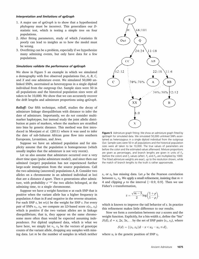
Interpretation and limitations of qpGraph

1. A major use of qpGraph is to show that a hypothesizedphylogeny must be incorrect. This generalizes our D-statistic test, which is testing a simple tree on fourpopulations.

2. After fitting parameters, study of which f-statistics fitpoorly can lead to insights as to how the model mustbe wrong.

3. Overfitting can be a problem, especially if we hypothesizemany admixing events, but only have data for a fewpopulations.

Simulations validate the performance of qpGraph

We show in Figure 5 an example in which we simulateda demography with five observed populations Out, A, B, C,and X and one admixture event. We simulated 50,000 un-linked SNPs, ascertained as heterozygous in a single diploidindividual from the outgroup Out. Sample sizes were 50 inall populations and the historical population sizes were alltaken to be 10,000. We show that we can accurately recoverthe drift lengths and admixture proportions using qpGraph.

Rolloff: Our fifth technique, rolloff, studies the decay ofadmixture linkage disequilibrium with distance to infer thedate of admixture. Importantly, we do not consider multi-marker haplotypes, but instead study the joint allelic distri-bution at pairs of markers, where the markers are stratifiedinto bins by genetic distance. This method was first intro-duced in Moorjani et al. (2011) where it was used to inferthe date of sub-Saharan African gene flow into southernEuropeans, Levantines, and Jews.

Suppose we have an admixed population and for sim-plicity assume that the population is homogeneous (whichusually implies that the admixture is not very recent).

Let us also assume that admixture occurred over a veryshort time span (pulse admixture model), and since then ouradmixed (target) population has not experienced furtherlarge-scale immigration from the source populations. Callthe two admixing (ancestral) populations A, B. Consider twoalleles on a chromosome in an admixed individual at locithat are a distance d apart. Then n generations after admix-ture, with probability e2nd the two alleles belonged, at theadmixing time, to a single chromosome.

Suppose we have a weight function w at each SNP that ispositive when the variant allele has a higher frequency inpopulation A than in B and negative in the reverse situation.For each SNP s, let w(s) be the weight for SNP s. For everypair of SNPs s1, s2, we compute an LD-based score z(s1, s2)which is positive if the two variant alleles are in linkagedisequilibrium; that is, they appear on the same chromo-some more often than would be expected assuming inde-pendence. For diploid unphased data, which is what wehave here, we simply let v1, v2 be the vectors of genotypecounts of the variant allele, dropping any samples with miss-ing data. Let m be the number of samples in which neither

s1 or s2 has missing data. Let r be the Pearson correlationbetween v1, v2. We apply a small refinement, insisting thatm$

4 and clipping r to the interval [20.9, 0.9]. Then we useFisher’s z-transformation,

z ¼ffiffiffiffiffiffiffiffiffiffiffiffiffim2 3

p

2log

�1þ r

12 r

�;

which is known to improve the tail behavior of z. In practicethis refinement makes little difference to our results.

Now we form a correlation between our z-scores and theweight function. Explicitly, for a bin-width x, define the “bin”S(d), d = x, 2x, 3x,. . . by the set of SNP pairs (s1, s2), where

SðdÞ ¼ fðs1; s2Þjd2 x, u2 2u1# dg;

where ui is the genetic position of SNP si.

Figure 5 Admixture graph fitting: We show an admixture graph fitted byqpGraph for simulated data. We simulated 50,000 unlinked SNPs ascer-tained as heterozygous in a single diploid individual from the outgroupOut. Sample sizes were 50 in all populations and the historical populationsizes were all taken to be 10,000. The true values of parameters arebefore the colon and the estimated values afterward. Mixture proportionsare given as percentages, and branch lengths are given in units of Fst(before the colon) and f2 values (after). F2 and Fst are multiplied by 1000.The fitted admixture weights are exact, up to the resolution shown, whilethe match of branch lengths to the truth is rather approximate.

Ancient Admixture 1075

Then we define A(d) to be the correlation coefficient

AðdÞ ¼P

s1;s22SðdÞwðs1Þwðs2Þzðs1; s2ÞhPs1;s22SðdÞðwðs1Þwðs2ÞÞ2

Ps1;s22SðdÞðzðs1; s2ÞÞ2

i1=2:

(8)

Here in both numerator and denominator we sum over pairsof SNPs approximately d units apart (counting SNP pairsinto discrete bins). In this study, we set a bin size of 0.1cM in all our examples. In practice, different choices of binsizes only qualitatively affect the results (Moorjani et al.2011).

Having computed A(d) over a suitable distance range, we fit

AðdÞ � A0e2nd (9)

by least squares and interpret n as an admixture date ingenerations. Equation 9 follows because a recombinationevent on a chromosome since admixture decorrelates thealleles at the two SNPs being considered, and e2nd is theprobability that no such event occurred. (Implicitly, we as-sume here that the number of recombinations over a geneticinterval of d in n generations is Poisson distributed withmean nd. Because of crossover interference, this is not exact,but it is an excellent approximation for the d and n relevanthere.)

By fitting a single exponential distribution to the output,we have assumed a single pulse model of admixture.However, in the case of continuous migration we can expectthe recovered date to lie within the time period spanned bythe start and end of the admixture events. We furtherdiscuss rolloff date estimates in the context of continuousmigration in applications to real data (below). We estimatestandard errors using a weighted block jackknife (Businget al. 1999) where we drop one chromosome in each run.

Choice of weight function

In many applications, we have access to two modernpopulations A, B, which we can regard as surrogates for thetrue admixing populations, and in this context we can simplyuse the difference of empirical frequencies of the variantallele as our weight. For example, to study the admixturein African Americans, very good surrogates for the ancestralpopulations are Yoruba and North Europeans. However,a strength of rolloff is that it provides unbiased dates evenwithout access to accurate surrogates for the ancestral pop-ulations. That is, rolloff is robust to use of highly divergentpopulations as surrogates. In cases when the ancestrals areno longer extant or data from the ancestrals are not available,but we have access to multiple admixed populations withdiffering admixture proportions (as for instance happens inIndia (Reich et al. 2009), we can use the “SNP loadings”generated from principal component analysis (PCA) as ap-propriate weights. This also gives unbiased dates for the ad-mixture events.

Simulations to test rolloff

We ran three sets of simulations. The goals of thesesimulations were

1. to access the accuracy of the estimated dates, in cases forwhich data from accurate ancestral populations are notavailable,

2. to investigate the bias seen in Moorjani et al. (2011),3. to test the effect of genetic drift that occurred after

admixture.

We describe the results of each of these investigations in turn.

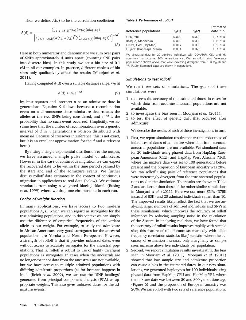
1. First, we report simulation results that test the robustness ofinferences of dates of admixture when data from accurateancestral populations are not available. We simulated datafor 20 individuals using phased data from HapMap Euro-pean Americans (CEU) and HapMap West Africans (YRI),where the mixture date was set to 100 generations beforepresent and the proportion of European ancestry was 20%.We ran rolloff using pairs of reference populations thatwere increasingly divergent from the true ancestral popula-tions used in the simulation. The results are shown in Table2 and are better than those of the rather similar simulationsin Moorjani et al. (2011). Here we use more SNPs (378Kinstead of 83K) and 20 admixed individuals rather than 10.The improved results likely reflect the fact that we are an-alyzing larger numbers of admixed individuals and SNPs inthese simulations, which improves the accuracy of rolloffinferences by reducing sampling noise in the calculationof the Z-score. In analyzing real data, we have found thatthe accuracy of rolloff results improves rapidly with samplesize; this feature of rolloff contrasts markedly with allelefrequency correlation statistics like f-statistics where the ac-curacy of estimation increases only marginally as samplesizes increase above five individuals per population.

2. Second, we report simulation results investigating the biasseen in Moorjani et al. (2011). Moorjani et al. (2011)showed that low sample size and admixture proportioncan cause a bias in the estimated dates. In our new simu-lations, we generated haplotypes for 100 individuals usingphased data from HapMap CEU and HapMap YRI, wherethe mixture date was between 50 and 800 generations ago(Figure 6) and the proportion of European ancestry was20%.We ran rolloff with two sets of reference populations:

Table 2 Performance of rolloff

Reference populations Fst(1) Fst(2)Estimateddate 6 SE

CEU, YRI 0.000 0.000 107 6 4Basque, Mandenka 0.009 0.009 106 6 4Druze, LWK(HapMap) 0.017 0.008 105 6 4Gujarati(HapMap), Maasai 0.034 0.026 107 6 4

We simulated data for 20 admixed individuals with 20%/80% CEU and YRIadmixture that occurred 100 generations ago. We ran rolloff using “referencepopulations” shown above that were increasing divergent from CEU (Fst(1)) andYRI (Fst(2)). Estimated dates are shown in generations.

1076 N. Patterson et al.

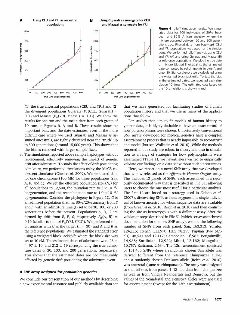
(1) the true ancestral populations (CEU and YRI) and (2)the divergent populations Gujarati (Fst(CEU, Gujarati) =0.03 and Maasai (Fst(YRI, Maasai) = 0.03). We show theresults for one run and the mean date from each group of10 runs in Figures 6, A and B. These results show noimportant bias, and the date estimates, even in the moredifficult case where we used Gujarati and Maasai as as-sumed ancestrals, are tightly clustered near the “truth” upto 500 generations (around 15,000 years). This shows thatthe bias is removed with larger sample sizes.

3. The simulations reported above sample haplotypes withoutreplacement, effectively removing the impact of geneticdrift after admixture. To study the effect of drift post-datingadmixture, we performed simulations using the MaCS co-alescent simulator (Chen et al. 2009). We simulated datafor one chromosome (100 Mb) for three populations (say,A, B, and C). We set the effective population size (Ne) forall populations to 12,500, the mutation rate to 2 · 1028/bp/generation, and the recombination rate to 1.0 · 1028/bp/generation. Consider the phylogeny in Figure 1C. G isan admixed population that has 80%/20% ancestry from Eand F, with an admixture time (t) set to be 30, 100, or 200generations before the present. Populations A, B, C areformed by drift from E, F, G, respectively. Fst(A, B) =0.16 (similar to that of Fst(YRI, CEU)). We performed roll-off analysis with C as the target (n = 30) and A and B asthe reference populations. We estimated the standard errorusing a weighted block jackknife where the block size wasset to 10 cM. The estimated dates of admixture were 28 64, 97 6 10, and 212 6 19 corresponding the true admix-ture dates of 30, 100, and 200 generations, respectively.This shows that the estimated dates are not measurablyaffected by genetic drift post-dating the admixture event.

A SNP array designed for population genetics

We conclude our presentation of our methods by describinga new experimental resource and publicly available data set

that we have generated for facilitating studies of humanpopulation history and that we use in many of the applica-tions that follow.

For studies that aim to fit models of human history togenetic data, it is highly desirable to have an exact record ofhow polymorphisms were chosen. Unfortunately, conventionalSNP arrays developed for medical genetics have a complexascertainment process that is nearly impossible to reconstructand model (but see Wollstein et al. 2010). While the methodsreported in our study are robust in theory and also in simula-tion to a range of strategies for how polymorphisms wereascertained (Table 1), we nevertheless wished to empiricallyvalidate our findings on a data set without such uncertainties.

Here, we report on a novel SNP array that we developedthat is now released as the Affymetrix Human Origins array.This includes 13 panels of SNPs, each ascertained in a rigor-ously documented way that is described in File S1, allowingusers to choose the one most useful for a particular analysis.The first 12 are based on a strategy used in Keinan et al.(2007), discovering SNPs as heterozygotes in a single individ-ual of known ancestry for whom sequence data are available(from Green et al. 2010; Reich et al. 2010) and then confirm-ing the site as heterozygous with a different assay. After thevalidation steps described in File S1 (which serves as technicaldocumentation for the new SNP array), we had the followingnumber of SNPs from each panel: San, 163,313; Yoruba,124,115; French, 111,970; Han, 78,253; Papuan (two pan-els), 48,531 and 12,117; Cambodian, 16,987; Bougainville,14,988; Sardinian, 12,922; Mbuti, 12,162; Mongolian,10,757; Karitiana, 2,634. The 13th ascertainment consistedof 151,435 SNPs where a randomly chosen San allele wasderived (different from the reference Chimpanzee allele)and a randomly chosen Denisova allele (Reich et al. 2010)was ancestral (same as chimpanzee). The array was designedso that all sites from panels 1–13 had data from chimpanzeeas well as from Vindija Neandertals and Denisova, but thevalues of the Neandertal and Denisova alleles were not usedfor ascertainment (except for the 13th ascertainment).

Figure 6 rolloff simulation results: We simu-lated data for 100 individuals of 20% Euro-pean and 80% African ancestry, where themixture occurred between 50 and 800 gener-ations ago. Phased data from HapMap3 CEUand YRI populations was used for the simula-tions. We performed rolloff analysis using CEUand YRI (A) and using Gujarati and Maasai (B)as reference populations. We plot the true dateof mixture (dotted line) against the estimateddate computed by rolloff (points in blue A andgreen B). Standard errors were calculated usingthe weighted block jackknife. To test the biasin the estimated dates, we repeated each sim-ulation 10 times. The estimated date based onthe 10 simulations is shown in red.

Ancient Admixture 1077

Throughout the design process, we avoided sources of biasthat could cause inferences to be affected by genetic datafrom human samples other than the discovery individual. Ouridentification of candidate SNPs was carried out entirelyusing sequencing reads mapped to the chimpanzee genome(PanTro2), so that we were not biased by the ancestry of thehuman reference sequence. In addition, we designed assaysblinded to prior information on the positions of polymor-phisms and did not take advantage of prior work that Affy-metrix had done to optimize assays for SNPs already reportedin databases. After initial testing of 1,353,671 SNPs on twoscreening arrays, we filtered to a final set of 542,399 SNPsthat passed all quality-control criteria. We also added a set of84,044 “compatibility SNPs” that were chosen to have a highoverlap with SNPs previously included on standard Affyme-trix and Illumina arrays, to facilitate coanalysis with datacollected on other SNP arrays. The final array contains629,443 unique and validated SNPs, and its technical detailsare described in File S1.

We successfully genotyped the array in 934 samples fromthe HGDP and made the data publicly available on August 12,2011, at ftp://ftp.cephb.fr/hgdp_supp10/. The present studyanalyzes a curated version of this data set in which we haveused principal component analysis (Patterson et al. 2006) toremove samples that are outliers relative to others from theirsame populations; 828 samples remained after this proce-dure. This curated data set is available for download fromthe Reich laboratory website (http://genetics.med.harvard.edu/reich/Reich_Lab/Datasets.html).

Results and Discussion

Initial application to data: South African Xhosa

The Xhosa are a South African population whose ancestorsare mostly Bantu speakers from the Nguni group, althoughthey also have some Bushman ancestors (Patterson et al.2010). We first ran our three-population test with San(HGDP) (Cann et al. 2002) and Yoruba (HapMap) (Interna-tional Hapmap 3 Consortium 2010) as source populationsand 20 samples of Xhosa as the target population, a sampleset already described in Patterson et al. (2010). We obtain anf3-statistic of 20.009 with a Z-score of 233.5, as computedwith the weighted block jackknife (Busing et al. 1999).

Note that the admixing Bantu-speaking population isknown to have been Nguni and certainly was not NigerianYoruba. However, as explained earlier, this is not crucial, ifthe actual admixing population is related genetically (Bantuspeakers have an ancient origin in West Africa). If a is theadmixing proportion of San here, we obtain using ourbounding technique with Han Chinese as an outgroup,

0:19#a# 0:55:

Although this interval is wide, it does show that the Bushmenhave made a major contribution to Xhosa genomes.

Xhosa: rolloff

We then applied our rolloff technique, using San and Yorubaas the reference populations, obtaining a very clear expo-nential admixture LD curve (Figure 7A). We estimate a dateof 25.36 1.1 generations, yielding a date of about 7406 30years before present (YBP) assuming 29 years per genera-tion (we also assume this generation time in the analysesthat follow) (Fenner 2005).

Archeological and linguistic evidence show that the Nguniare a population that migrated south from the Great Lakesarea of East Africa. For the dating of the migration we quote:

From an archaeological perspective, the first appearance ofNguni speakers can be recognized by a break in ceramicstyle; the Nguni style is quite different from the Early IronAge sequence in the area. This break is dated to about AD1200 (Huffman 2010).

More detail on Nguni migrations and archeology can befound in Huffman (2004).

Our date is slightly more recent than the dates obtained fromthe archeology, but very reasonable, since gene flow from theBushmen into the Nguni plausibly continued after initial contact.

Admixture of the Uygur

The Uygur are known to be historically admixed, but wewanted to try our methods on them. We analyzed a smallsample (nine individuals from HGDP) (Cann et al. 2002). Ourthree-population test using French and Japanese as sourcesand Uygur as target gives a Z-score of 276.1, a remarkablysignificant value. Exploring this a little further, we get theresults shown in Table 3.

Using Han instead of Japanese is historically moreplausible and statistically not significantly different. Ourbounding methods suggest that the West Eurasian admix-ture a is in the range

0:452#a# 0:525:

We used French and Han for the source populations here.Russian as a source is significantly weaker than French. Webelieve that the likely reason is that our Russian sampleshave more gene flow from East Asia than the Frenchsamples, and this weakens the signal. We confirm this byfinding that D(Yoruba, Han; French, Russian) = 0.192, Z =26.3. The fact that we obtain very similar statistics when wesubstitute a very different sub-Saharan African population(HGDP San) for Yoruba (D= 0.189, Z= 23.9) indicates thatthe gene flow does not involve an African population, andinstead the findings reflect gene flow between relatives ofthe Han and Russians.

Uygur: rolloff

Applying rolloff we again get a very clear decay curve(Figure 7B). We estimate a date of 790 6 60 YBP.

Uygur genetics has been analyzed in two articles by Xu,Jin, and colleagues (Xu et al. 2008; Xu and Jin 2008), using

1078 N. Patterson et al.

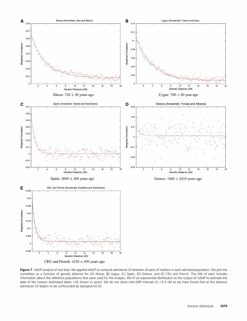
Figure 7 rolloff analysis of real data: We applied rolloff to compute admixture LD between all pairs of markers in each admixed population. We plot thecorrelation as a function of genetic distance for (A) Xhosa, (B) Uygur, (C) Spain, (D) Greece, and (E) CEU and French. The title of each includesinformation about the reference populations that were used for the analysis. We fit an exponential distribution to the output of rolloff to estimate thedate of the mixture (estimated dates 6SE shown in years). We do not show inter-SNP intervals of ,0.5 cM as we have found that at this distanceadmixture LD begins to be confounded by background LD.

Ancient Admixture 1079

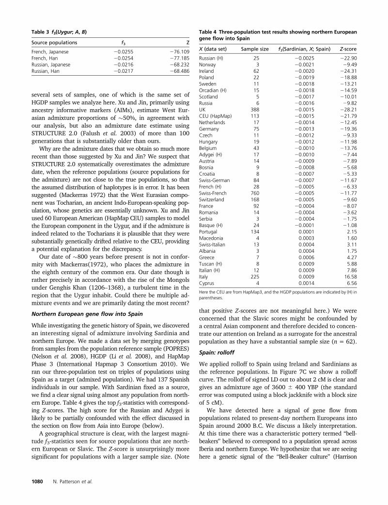
several sets of samples, one of which is the same set ofHGDP samples we analyze here. Xu and Jin, primarily usingancestry informative markers (AIMs), estimate West Eur-asian admixture proportions of �50%, in agreement withour analysis, but also an admixture date estimate usingSTRUCTURE 2.0 (Falush et al. 2003) of more than 100generations that is substantially older than ours.

Why are the admixture dates that we obtain so much morerecent than those suggested by Xu and Jin? We suspect thatSTRUCTURE 2.0 systematically overestimates the admixturedate, when the reference populations (source populations forthe admixture) are not close to the true populations, so thatthe assumed distribution of haplotypes is in error. It has beensuggested (Mackerras 1972) that the West Eurasian compo-nent was Tocharian, an ancient Indo-European-speaking pop-ulation, whose genetics are essentially unknown. Xu and Jinused 60 European American (HapMap CEU) samples to modelthe European component in the Uygur, and if the admixture isindeed related to the Tocharians it is plausible that they weresubstantially genetically drifted relative to the CEU, providinga potential explanation for the discrepancy.

Our date of �800 years before present is not in confor-mity with Mackerras(1972), who places the admixture inthe eighth century of the common era. Our date though israther precisely in accordance with the rise of the Mongolsunder Genghis Khan (1206–1368), a turbulent time in theregion that the Uygur inhabit. Could there be multiple ad-mixture events and we are primarily dating the most recent?

Northern European gene flow into Spain

While investigating the genetic history of Spain, we discoveredan interesting signal of admixture involving Sardinia andnorthern Europe. We made a data set by merging genotypesfrom samples from the population reference sample (POPRES)(Nelson et al. 2008), HGDP (Li et al. 2008), and HapMapPhase 3 (International Hapmap 3 Consortium 2010). Weran our three-population test on triples of populations usingSpain as a target (admixed population). We had 137 Spanishindividuals in our sample. With Sardinian fixed as a source,we find a clear signal using almost any population from north-ern Europe. Table 4 gives the top f3-statistics with correspond-ing Z-scores. The high score for the Russian and Adygei islikely to be partially confounded with the effect discussed inthe section on flow from Asia into Europe (below).

A geographical structure is clear, with the largest magni-tude f3-statistics seen for source populations that are north-ern European or Slavic. The Z-score is unsurprisingly moresignificant for populations with a larger sample size. (Note

that positive Z-scores are not meaningful here.) We wereconcerned that the Slavic scores might be confounded bya central Asian component and therefore decided to concen-trate our attention on Ireland as a surrogate for the ancestralpopulation as they have a substantial sample size (n = 62).

Spain: rolloff

We applied rolloff to Spain using Ireland and Sardinians asthe reference populations. In Figure 7C we show a rolloffcurve. The rolloff of signed LD out to about 2 cM is clear andgives an admixture age of 3600 6 400 YBP (the standarderror was computed using a block jackknife with a block sizeof 5 cM).

We have detected here a signal of gene flow frompopulations related to present-day northern Europeans intoSpain around 2000 B.C. We discuss a likely interpretation.At this time there was a characteristic pottery termed “bell-beakers” believed to correspond to a population spread acrossIberia and northern Europe. We hypothesize that we are seeinghere a genetic signal of the “Bell-Beaker culture” (Harrison

Table 3 f3(Uygur; A, B)

Source populations f3 Z

French, Japanese 20.0255 276.109French, Han 20.0254 277.185Russian, Japanese 20.0216 268.232Russian, Han 20.0217 268.486

Table 4 Three-population test results showing northern Europeangene flow into Spain

X (data set) Sample size f3(Sardinian, X; Spain) Z-score

Russian (H) 25 20.0025 222.90Norway 3 20.0021 29.49Ireland 62 20.0020 224.31Poland 22 20.0019 218.88Sweden 11 20.0018 213.21Orcadian (H) 15 20.0018 214.59Scotland 5 20.0017 210.01Russia 6 20.0016 29.82UK 388 20.0015 228.21CEU (HapMap) 113 20.0015 221.79Netherlands 17 20.0014 212.45Germany 75 20.0013 219.36Czech 11 20.0012 29.33Hungary 19 20.0012 211.98Belgium 43 20.0010 213.76Adygei (H) 17 20.0010 27.44Austria 14 20.0009 27.89Bosnia 9 20.0008 25.68Croatia 8 20.0007 25.33Swiss-German 84 20.0007 211.67French (H) 28 20.0005 26.33Swiss-French 760 20.0005 211.77Switzerland 168 20.0005 29.60France 92 20.0004 28.07Romania 14 20.0004 23.62Serbia 3 20.0004 21.75Basque (H) 24 20.0001 21.08Portugal 134 0.0001 2.15Macedonia 4 0.0003 1.60Swiss-Italian 13 0.0004 3.11Albania 3 0.0004 1.75Greece 7 0.0006 4.27Tuscan (H) 8 0.0009 5.88Italian (H) 12 0.0009 7.86Italy 225 0.0009 16.58Cyprus 4 0.0014 6.56

Here the CEU are from HapMap3, and the HGDP populations are indicated by (H) inparentheses.

1080 N. Patterson et al.

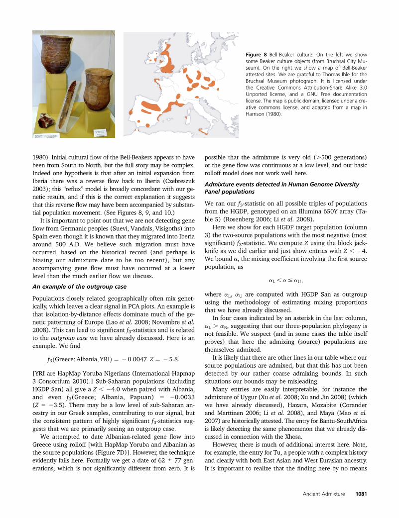
1980). Initial cultural flow of the Bell-Beakers appears to havebeen from South to North, but the full story may be complex.Indeed one hypothesis is that after an initial expansion fromIberia there was a reverse flow back to Iberia (Czebreszuk2003); this “reflux” model is broadly concordant with our ge-netic results, and if this is the correct explanation it suggeststhat this reverse flow may have been accompanied by substan-tial population movement. (See Figures 8, 9, and 10.)

It is important to point out that we are not detecting geneflow from Germanic peoples (Suevi, Vandals, Visigoths) intoSpain even though it is known that they migrated into Iberiaaround 500 A.D. We believe such migration must haveoccurred, based on the historical record (and perhaps isbiasing our admixture date to be too recent), but anyaccompanying gene flow must have occurred at a lowerlevel than the much earlier flow we discuss.

An example of the outgroup case

Populations closely related geographically often mix genet-ically, which leaves a clear signal in PCA plots. An example isthat isolation-by-distance effects dominate much of the ge-netic patterning of Europe (Lao et al. 2008; Novembre et al.2008). This can lead to significant f3-statistics and is relatedto the outgroup case we have already discussed. Here is anexample. We find

f3ðGreece; Albania;YRIÞ ¼ 2 0:0047 Z ¼ 25:8:

[YRI are HapMap Yoruba Nigerians (International Hapmap3 Consortium 2010).] Sub-Saharan populations (includingHGDP San) all give a Z , 24.0 when paired with Albania,and even f3(Greece; Albania, Papuan) = 20.0033(Z = 23.5). There may be a low level of sub-Saharan an-cestry in our Greek samples, contributing to our signal, butthe consistent pattern of highly significant f3-statistics sug-gests that we are primarily seeing an outgroup case.

We attempted to date Albanian-related gene flow intoGreece using rolloff [with HapMap Yoruba and Albanian asthe source populations (Figure 7D)]. However, the techniqueevidently fails here. Formally we get a date of 62 6 77 gen-erations, which is not significantly different from zero. It is

possible that the admixture is very old (.500 generations)or the gene flow was continuous at a low level, and our basicrolloff model does not work well here.

Admixture events detected in Human Genome DiversityPanel populations

We ran our f3-statistic on all possible triples of populationsfrom the HGDP, genotyped on an Illumina 650Y array (Ta-ble 5) (Rosenberg 2006; Li et al. 2008).

Here we show for each HGDP target population (column3) the two-source populations with the most negative (mostsignificant) f3-statistic. We compute Z using the block jack-knife as we did earlier and just show entries with Z , 24.We bound a, the mixing coefficient involving the first sourcepopulation, as

aL ,a#aU;

where aL, aU are computed with HGDP San as outgroupusing the methodology of estimating mixing proportionsthat we have already discussed.

In four cases indicated by an asterisk in the last column,aL . aR, suggesting that our three-population phylogeny isnot feasible. We suspect (and in some cases the table itselfproves) that here the admixing (source) populations arethemselves admixed.

It is likely that there are other lines in our table where oursource populations are admixed, but that this has not beendetected by our rather coarse admixing bounds. In suchsituations our bounds may be misleading.

Many entries are easily interpretable, for instance theadmixture of Uygur (Xu et al. 2008; Xu and Jin 2008) (whichwe have already discussed), Hazara, Mozabite (Coranderand Marttinen 2006; Li et al. 2008), and Maya (Mao et al.2007) are historically attested. The entry for Bantu-SouthAfricais likely detecting the same phenomenon that we already dis-cussed in connection with the Xhosa.

However, there is much of additional interest here. Note,for example, the entry for Tu, a people with a complex historyand clearly with both East Asian and West Eurasian ancestry.It is important to realize that the finding here by no means

Figure 8 Bell-Beaker culture. On the left we showsome Beaker culture objects (from Bruchsal City Mu-seum). On the right we show a map of Bell-Beakerattested sites. We are grateful to Thomas Ihle for theBruchsal Museum photograph. It is licensed underthe Creative Commons Attribution-Share Alike 3.0Unported license, and a GNU Free documentationlicense. The map is public domain, licensed under a cre-ative commons license, and adapted from a map inHarrison (1980).

Ancient Admixture 1081

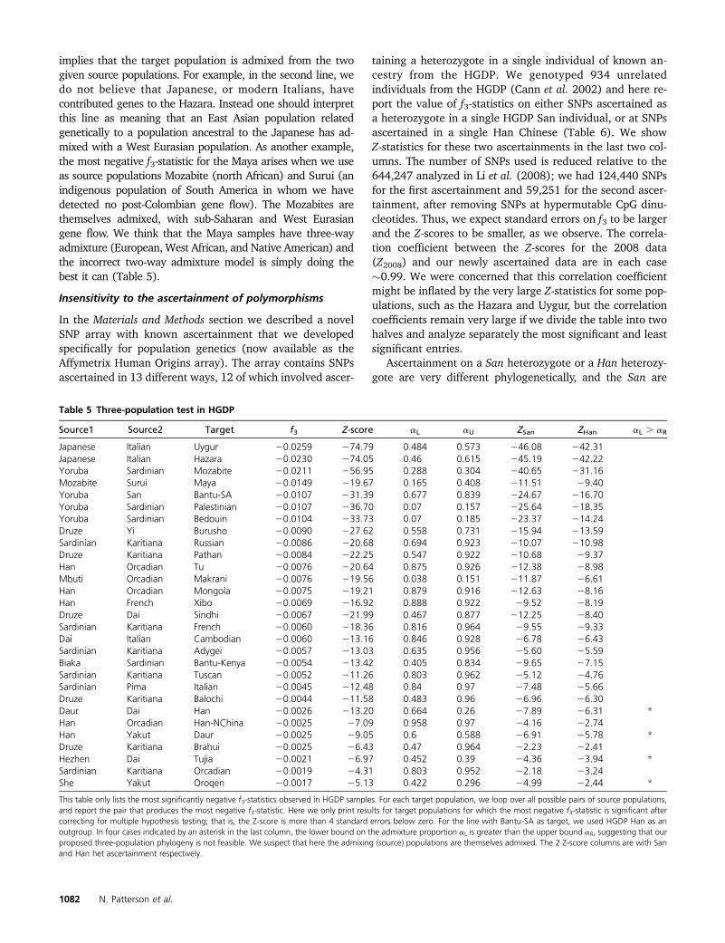
implies that the target population is admixed from the twogiven source populations. For example, in the second line, wedo not believe that Japanese, or modern Italians, havecontributed genes to the Hazara. Instead one should interpretthis line as meaning that an East Asian population relatedgenetically to a population ancestral to the Japanese has ad-mixed with a West Eurasian population. As another example,the most negative f3-statistic for the Maya arises when we useas source populations Mozabite (north African) and Surui (anindigenous population of South America in whom we havedetected no post-Colombian gene flow). The Mozabites arethemselves admixed, with sub-Saharan and West Eurasiangene flow. We think that the Maya samples have three-wayadmixture (European, West African, and Native American) andthe incorrect two-way admixture model is simply doing thebest it can (Table 5).

Insensitivity to the ascertainment of polymorphisms

In the Materials and Methods section we described a novelSNP array with known ascertainment that we developedspecifically for population genetics (now available as theAffymetrix Human Origins array). The array contains SNPsascertained in 13 different ways, 12 of which involved ascer-

taining a heterozygote in a single individual of known an-cestry from the HGDP. We genotyped 934 unrelatedindividuals from the HGDP (Cann et al. 2002) and here re-port the value of f3-statistics on either SNPs ascertained asa heterozygote in a single HGDP San individual, or at SNPsascertained in a single Han Chinese (Table 6). We showZ-statistics for these two ascertainments in the last two col-umns. The number of SNPs used is reduced relative to the644,247 analyzed in Li et al. (2008); we had 124,440 SNPsfor the first ascertainment and 59,251 for the second ascer-tainment, after removing SNPs at hypermutable CpG dinu-cleotides. Thus, we expect standard errors on f3 to be largerand the Z-scores to be smaller, as we observe. The correla-tion coefficient between the Z-scores for the 2008 data(Z2008) and our newly ascertained data are in each case�0.99. We were concerned that this correlation coefficientmight be inflated by the very large Z-statistics for some pop-ulations, such as the Hazara and Uygur, but the correlationcoefficients remain very large if we divide the table into twohalves and analyze separately the most significant and leastsignificant entries.

Ascertainment on a San heterozygote or a Han heterozy-gote are very different phylogenetically, and the San are

Table 5 Three-population test in HGDP

Source1 Source2 Target f3 Z-score aL aU ZSan ZHan aL . aR

Japanese Italian Uygur 20.0259 274.79 0.484 0.573 246.08 242.31Japanese Italian Hazara 20.0230 274.05 0.46 0.615 245.19 242.22Yoruba Sardinian Mozabite 20.0211 256.95 0.288 0.304 240.65 231.16Mozabite Surui Maya 20.0149 219.67 0.165 0.408 211.51 29.40Yoruba San Bantu-SA 20.0107 231.39 0.677 0.839 224.67 216.70Yoruba Sardinian Palestinian 20.0107 236.70 0.07 0.157 225.64 218.35Yoruba Sardinian Bedouin 20.0104 233.73 0.07 0.185 223.37 214.24Druze Yi Burusho 20.0090 227.62 0.558 0.731 215.94 213.59Sardinian Karitiana Russian 20.0086 220.68 0.694 0.923 210.07 210.98Druze Karitiana Pathan 20.0084 222.25 0.547 0.922 210.68 29.37Han Orcadian Tu 20.0076 220.64 0.875 0.926 212.38 28.98Mbuti Orcadian Makrani 20.0076 219.56 0.038 0.151 211.87 26.61Han Orcadian Mongola 20.0075 219.21 0.879 0.916 212.63 28.16Han French Xibo 20.0069 216.92 0.888 0.922 29.52 28.19Druze Dai Sindhi 20.0067 221.99 0.467 0.877 212.25 28.40Sardinian Karitiana French 20.0060 218.36 0.816 0.964 29.55 29.33Dai Italian Cambodian 20.0060 213.16 0.846 0.928 26.78 26.43Sardinian Karitiana Adygei 20.0057 213.03 0.635 0.956 25.60 25.59Biaka Sardinian Bantu-Kenya 20.0054 213.42 0.405 0.834 29.65 27.15Sardinian Karitiana Tuscan 20.0052 211.26 0.803 0.962 25.12 24.76Sardinian Pima Italian 20.0045 212.48 0.84 0.97 27.48 25.66Druze Karitiana Balochi 20.0044 211.58 0.483 0.96 26.96 26.30Daur Dai Han 20.0026 213.20 0.664 0.26 27.89 26.31 *Han Orcadian Han-NChina 20.0025 27.09 0.958 0.97 24.16 22.74Han Yakut Daur 20.0025 29.05 0.6 0.588 26.91 25.78 *Druze Karitiana Brahui 20.0025 26.43 0.47 0.964 22.23 22.41Hezhen Dai Tujia 20.0021 26.97 0.452 0.39 24.36 23.94 *Sardinian Karitiana Orcadian 20.0019 24.31 0.803 0.952 22.18 23.24She Yakut Oroqen 20.0017 25.13 0.422 0.296 24.99 22.44 *

This table only lists the most significantly negative f3-statistics observed in HGDP samples. For each target population, we loop over all possible pairs of source populations,and report the pair that produces the most negative f3-statistic. Here we only print results for target populations for which the most negative f3-statistic is significant aftercorrecting for multiple hypothesis testing; that is, the Z-score is more than 4 standard errors below zero. For the line with Bantu-SA as target, we used HGDP Han as anoutgroup. In four cases indicated by an asterisk in the last column, the lower bound on the admixture proportion aL is greater than the upper bound aR, suggesting that ourproposed three-population phylogeny is not feasible. We suspect that here the admixing (source) populations are themselves admixed. The 2 Z-score columns are with Sanand Han het ascertainment respectively.

1082 N. Patterson et al.

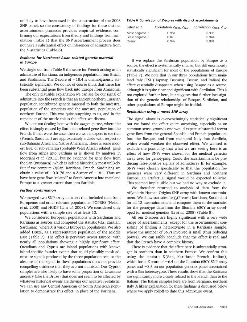
unlikely to have been used in the construction of the 2008SNP panel, so the consistency of findings for these distinctascertainment processes provides empirical evidence, con-firming our expectations from theory and findings from sim-ulation (Table 1) that the SNP ascertainment process doesnot have a substantial effect on inferences of admixture fromthe f3-statistics (Table 6).

Evidence for Northeast Asian-related genetic materialin Europe

We single out from Table 5 the score for French arising as anadmixture of Karitiana, an indigenous population from Brazil,and Sardinians. The Z-score of 218.4 is unambiguously sta-tistically significant. We do not of course think that there hasbeen substantial gene flow back into Europe from Amazonia.

The only plausible explanation we can see for our signal ofadmixture into the French is that an ancient northern Eurasianpopulation contributed genetic material to both the ancestralpopulation of the Americas and the ancestral population ofnorthern Europe. This was quite surprising to us, and in theremainder of the article this is the effect we discuss.

We are not dealing here with the outgroup case, where theeffect is simply caused by Sardinian-related gene flow into theFrench. If that were the case, then we would expect to see that(French, Sardinian) are approximately a clade with respect tosub-Saharan Africa and Native Americans. There is some mod-est level of sub-Saharan (probably West African related) geneflow from Africa into Sardinia as is shown by analyses inMoorjani et al. (2011), but no evidence for gene flow fromthe San (Bushmen), which is indeed historically most unlikely.But if we compute D(San, Karitiana, French, Sardinian) weobtain a value of 20.0178 and a Z-score of 218.1. Thus wehave here gene flow “related” to South America into mainlandEurope to a greater extent than into Sardinia.

Further confirmation

We merged two SNP array data sets that included data fromEuropeans and other relevant populations: POPRES (Nelsonet al. 2008) and HGDP (Li et al. 2008). We considered onlypopulations with a sample size of at least 10.

We considered European populations with Sardinian andKaritiana as sources and computed the statistic f3(X; Karitian,Sardinian), where X is various European populations. We alsoadded Druze, as a representative population of the MiddleEast (Table 7). The effect is pervasive across Europe, withnearly all populations showing a highly significant effect.Orcadians and Cyprus are island populations with knownisland-specific founder events that could plausibly mask ad-mixture signals produced by the three-population test, so theabsence of the signal in these populations does not providecompelling evidence that they are not admixed. Our Cypriotsamples are also likely to have some proportion of Levantineancestry (like the Druze) that does not seem to be affected bywhatever historical events are driving our negative f3-statistic.We can use any Central American or South American popu-lation to demonstrate this effect, in place of the Karitiana.

If we replace the Sardinian population by Basque as asource, the effect is systematically smaller, but still enormouslystatistically significant for most of the populations of Europe(Table 7). We note that in our three populations from main-land Italy [TSI (Hapmap Tuscans), Tuscan, and Italian] theeffect essentially disappears when using Basque as a source,although it is quite clear and significant with Sardinian. This isnot explored further here, but suggests that further investiga-tion of the genetic relationships of Basque, Sardinian, andother populations of Europe might be fruitful.

Replication using a novel SNP array

The signal above is overwhelmingly statistically significantbut we found the effect quite surprising, especially as oncommon-sense grounds one would expect substantial recentgene flow from the general Spanish and French populationsinto the Basque, and from mainland Italy into Sardinia,which would weaken the observed effect. We wanted toexclude the possibility that what we are seeing here is aneffect of how SNPs were chosen for the medical geneticsarray used for genotyping. Could the ascertainment be pro-ducing false-positive signals of admixture? If, for example,SNPs were chosen specifically so that the population fre-quencies were very different in Sardinia and northernEurope, an artifactual signal would be expected to arise.This seemed implausible but we had no way to exclude it.

We therefore returned to analysis of data from theAffymetrix Human Origins SNP array with known ascertain-ment. We show statistics for f3(French; Karitiana, Saridinian)for all 13 ascertainments and compare them to the statisticsfor the genotype data from the Illumina 650Y array devel-oped for medical genetics (Li et al. 2008) (Table 8).

All our Z-scores are highly significant with a very widerange of ascertainments, except for the ascertainment con-sisting of finding a heterozygote in a Karitiana sample,where the number of SNPs involved is small (thus reducingpower). We can safely conclude that the effect is real andthat the French have a complex history.

There is evidence that the effect here is substantially stron-ger in northern than in southern Europe. We confirm thisusing the statistic D(San, Karitiana; French, Italian),which has a Z-score of 26.4 on the Illumina 650Y SNP arraypanel and 23.5 on our population genetics panel ascertainedwith a San heterozygote. These results show that the Karitianaare significantly more closely related to the French than to theItalians. The Italian samples here are from Bergamo, northernItaly. A likely explanation for these findings is discussed belowwhere we apply rolloff to date this admixture event.

Table 6 Correlation of Z-scores with distinct ascertainments

Selected Z Correlation Z2008, ZSan Correlation Z2008, ZHan

Most negative Z 0.981 0.995Least negative Z 0.875 0.944Overall 0.987 0.991

Ancient Admixture 1083

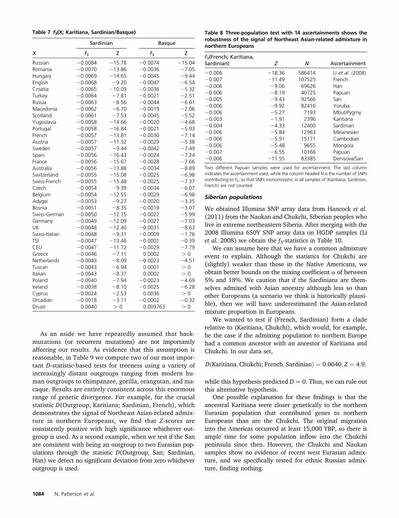
As an aside we have repeatedly assumed that back-mutations (or recurrent mutations) are not importantlyaffecting our results. As evidence that this assumption isreasonable, in Table 9 we compute two of our most impor-tant D-statistic-based tests for treeness using a variety ofincreasingly distant outgroups ranging from modern hu-man outgroups to chimpanzee, gorilla, orangutan, and ma-caque. Results are entirely consistent across this enormousrange of genetic divergence. For example, for the crucialstatistic D(Outgroup, Karitiana; Sardinian, French), whichdemonstrates the signal of Northeast Asian-related admix-ture in northern Europeans, we find that Z-scores areconsistently positive with high significance whichever out-group is used. As a second example, when we test if the Sanare consistent with being an outgroup to two Eurasian pop-ulations through the statistic D(Outgroup, San; Sardinian,Han) we detect no significant deviation from zero whicheveroutgroup is used.

Siberian populations

We obtained Illumina SNP array data from Hancock et al.(2011) from the Naukan and Chukchi, Siberian peoples wholive in extreme northeastern Siberia. After merging with the2008 Illumina 650Y SNP array data on HGDP samples (Liet al. 2008) we obtain the f3-statistics in Table 10.

We can assume here that we have a common admixtureevent to explain. Although the statistics for Chukchi are(slightly) weaker than those in the Native Americans, weobtain better bounds on the mixing coefficient a of between5% and 18%. We caution that if the Sardinians are them-selves admixed with Asian ancestry although less so thanother Europeans (a scenario we think is historically plausi-ble), then we will have underestimated the Asian-relatedmixture proportion in Europeans.

We wanted to test if (French, Sardinian) form a claderelative to (Karitiana, Chukchi), which would, for example,be the case if the admixing population to northern Europehad a common ancestor with an ancestor of Karitiana andChukchi. In our data set,

DðKaritiana;Chukchi; French; SardinianÞ ¼ 0:0040; Z ¼ 4:9;

while this hypothesis predicted D = 0. Thus, we can rule outthis alternative hypothesis.

One possible explanation for these findings is that theancestral Karitiana were closer genetically to the northernEurasian population that contributed genes to northernEuropeans than are the Chukchi. The original migrationinto the Americas occurred at least 15,000 YBP, so there isample time for some population inflow into the Chukchipeninsula since then. However, the Chukchi and Naukansamples show no evidence of recent west Eurasian admix-ture, and we specifically tested for ethnic Russian admix-ture, finding nothing.

Table 7 f3(X; Karitiana, Sardinian/Basque)

Sardinian Basque

X f3 Z f3 Z

Russian 20.0084 215.78 20.0074 215.04Romania 20.0070 213.86 20.0036 27.05Hungary 20.0069 214.65 20.0045 29.44English 20.0068 29.20 20.0047 26.54Croatia 20.0065 210.09 20.0036 25.32Turkey 20.0064 27.81 20.0021 22.51Russia 20.0063 28.56 20.0044 26.01Macedonia 20.0062 26.70 20.0019 22.06Scotland 20.0061 27.53 20.0045 25.52Yugoslavia 20.0058 214.66 20.0020 24.68Portugal 20.0058 216.84 20.0021 25.93French 20.0057 213.81 20.0030 27.14Austria 20.0057 211.32 20.0029 25.38Sweden 20.0057 29.44 20.0042 27.49Spain 20.0056 216.43 20.0024 27.24France 20.0056 215.67 20.0028 27.66Australia 20.0056 213.88 20.0034 28.89Switzerland 20.0055 215.08 20.0025 26.98Swiss-French 20.0055 215.48 20.0025 27.37Czech 20.0054 29.39 20.0034 26.07Belgium 20.0054 212.55 20.0029 26.98Adygei 20.0053 29.27 20.0020 23.35Bosnia 20.0051 28.35 20.0019 23.07Swiss-German 20.0050 212.75 20.0022 25.99Germany 20.0049 212.09 20.0027 27.03UK 20.0048 212.40 20.0031 28.63Swiss-Italian 20.0048 29.31 20.0009 21.76TSI 20.0047 213.46 20.0001 20.39CEU 20.0047 211.72 20.0029 27.79Greece 20.0046 27.11 0.0002 . 0Netherlands 20.0043 28.09 20.0023 24.51Tuscan 20.0043 26.94 0.0001 . 0Italian 20.0043 28.37 0.0002 . 0Poland 20.0040 27.94 20.0023 24.69Ireland 20.0038 28.10 20.0025 26.28Cyprus 20.0024 22.53 0.0036 . 0Orcadian 20.0018 23.11 20.0002 20.32Druze 0.0040 . 0 0.009763 . 0

Table 8 Three-population test with 14 ascertainments shows therobustness of the signal of Northeast Asian-related admixture innorthern Europeans

f3(French; Karitiana,Sardinian) Z N Ascertainment

20.006 218.36 586414 Li et al. (2008)20.007 211.49 107525 French20.006 29.06 69626 Han20.006 28.19 40725 Papuan20.005 29.43 92566 San20.006 29.92 82416 Yoruba20.006 25.27 7193 MbutiPygmy20.003 21.91 2396 Karitiana20.004 24.33 12400 Sardinian20.006 25.84 12963 Melanesian20.006 25.91 15171 Cambodian20.006 25.48 9655 Mongola20.007 26.55 10166 Papuan20.006 211.55 83385 Denisova/San

Two different Papuan samples were used for ascertainment. The last columnindicates the ascertainment used, while the column headed N is the number of SNPscontributing to f3, so that SNPs monomorphic in all samples of (Karitiana, Sardinian,French) are not counted.

1084 N. Patterson et al.

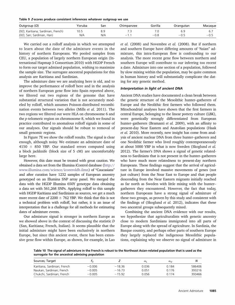
We carried out a rolloff analysis in which we attemptedto learn about the date of the admixture events in thehistory of northern Europeans. We pooled samples fromCEU, a population of largely northern European origin (In-ternational Hapmap 3 Consortium 2010) with HGDP Frenchto form our target admixed population, wishing to maximizethe sample size. The surrogate ancestral populations for thisanalysis are Karitiana and Sardinian.

The admixture date we are analyzing here is old, and toimprove the performance of rolloff here and in the analysisof northern European gene flow into Spain reported above,we filtered out two regions of the genome that havesubstantial structural variation that is not accurately mod-eled by rolloff, which assumes Poisson-distributed recombi-nation events between two alleles (Mills et al. 2011). Thetwo regions we filtered out were HLA on chromosome 6 andthe p-telomeric region on chromosome 8, which we found inpractice contributed to anomalous rolloff signals in some ofour analyses. Our signals should be robust to removal ofsmall genomic regions.

In Figure 7E we show the rolloff results. The signal is clearenough, although noisy. We estimate an admixture date of4150 6 850 YBP. Our standard errors computed usinga block jackknife (block size of 5 cM) are uncomfortablylarge here.

However, this date must be treated with great caution. Weobtained a data set from the Illumina iControl database (http://www.illumina.com/science/icontroldb.ilmn) of “Caucasians”and after curation have 1232 samples of European ancestrygenotyped on an Illumina SNP array panel. We merged thedata with the HGDP Illumina 650Y genotype data obtaininga data set with 561,268 SNPs. Applying rolloff to this samplewith HGDP Karitiana and Sardinians as sources, we get a muchmore recent date of 22006 762 YBP. We think that this is nota technical problem with rolloff, but rather, it is an issue ofinterpretation that is a challenge for all methods for estimatingdates of admixture events.

Our admixture signal is stronger in northern Europe aswe showed above in the context of discussing the statistic D(San, Karitiana; French, Italian). It seems plausible that theinitial admixture might have been exclusively in northernEurope, but since this ancient event, there has been exten-sive gene flow within Europe, as shown, for example, in Lao

et al. (2008) and Novembre et al. (2008). But if northernand southern Europe have differing amounts of “Asian” ad-mixture, this intra-European flow is confounding to ouranalysis. The more recent gene flow between northern andsouthern Europe will contribute to our inferring too recenta date. Admixture into one section of a population, followedby slow mixing within the population, may be quite commonin human history and will substantially complicate the dat-ing for any genetic method.

Interpretation in light of ancient DNA

Ancient DNA studies have documented a clean break betweenthe genetic structure of the Mesolithic hunter–gatherers ofEurope and the Neolithic first farmers who followed them.Mitochondrial analyses have shown that the first farmers incentral Europe, belonging to the linear pottery culture (LBK),were genetically strongly differentiated from Europeanhunter–gatherers (Bramanti et al. 2009), with an affinity topresent-day Near Eastern and Anatolian populations (Haaket al. 2010). More recently, new insight has come from anal-ysis of ancient nuclear DNA from three hunter–gatherers andone Neolithic farmer who lived roughly contemporaneouslyat about 5000 YBP in what is now Sweden (Skoglund et al.2012). The farmer’s DNA shows a signal of genetic related-ness to Sardinians that is not present in the hunter–gathererswho have much more relatedness to present-day northernEuropeans. These findings suggest that the arrival of agricul-ture in Europe involved massive movements of genes (notjust culture) from the Near East to Europe and that peopledescending from the Near Eastern migrants initially reachedas far north as Sweden with little mixing with the hunter–gatherers they encountered. However, the fact that today,northern Europeans have a strong signal of admixture ofthese two groups, as proven by this study and consistent withthe findings of (Skoglund et al. 2012), indicates that thesetwo ancestral groups subsequently mixed.

Combining the ancient DNA evidence with our results,we hypothesize that agriculturalists with genetic ancestryclose to modern Sardinians immigrated into all parts ofEurope along with the spread of agriculture. In Sardinia, theBasque country, and perhaps other parts of southern Europethey largely replaced the indigenous Mesolithic popula-tions, explaining why we observe no signal of admixture in

Table 9 Z-scores produce consistent inferences whatever outgroup we use

Outgroup (O) Yoruba San Chimpanzee Gorilla Orangutan Macaque

D(O, Karitiana; Sardinian, French) 10.5 8.9 7.3 7.0 6.9 6.7D(O, San; Sardinian, Han) N/A N/A 21.1 20.8 20.5 20.5

Table 10 The signal of admixture in the French is robust to the Northeast Asian-related population that is used as thesurrogate for the ancestral admixing population

Sources; Target f3 Z aL aU N

Karitiana, Sardinian; French 20.006 218.36 0.036 0.184 586406Naukan, Sardinian; French 20.005 216.73 0.051 0.176 393216Chukchi, Sardinian; French 20.005 215.92 0.056 0.174 393466

Ancient Admixture 1085

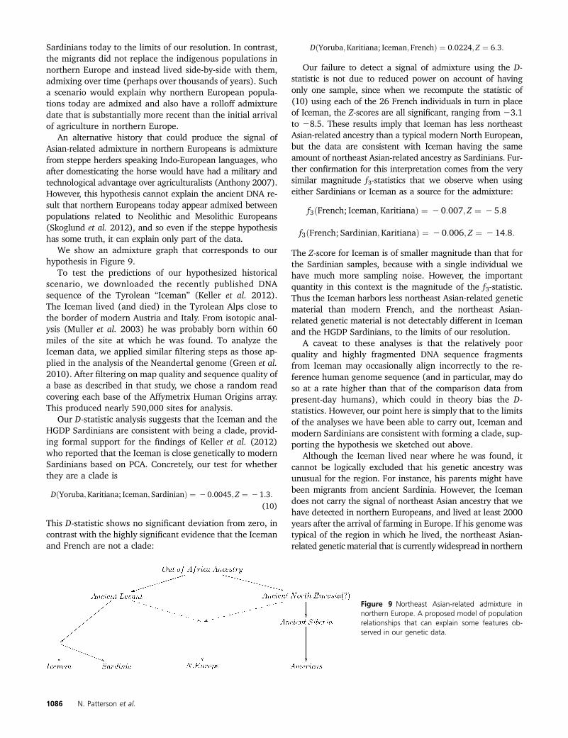
Sardinians today to the limits of our resolution. In contrast,the migrants did not replace the indigenous populations innorthern Europe and instead lived side-by-side with them,admixing over time (perhaps over thousands of years). Sucha scenario would explain why northern European popula-tions today are admixed and also have a rolloff admixturedate that is substantially more recent than the initial arrivalof agriculture in northern Europe.

An alternative history that could produce the signal ofAsian-related admixture in northern Europeans is admixturefrom steppe herders speaking Indo-European languages, whoafter domesticating the horse would have had a military andtechnological advantage over agriculturalists (Anthony 2007).However, this hypothesis cannot explain the ancient DNA re-sult that northern Europeans today appear admixed betweenpopulations related to Neolithic and Mesolithic Europeans(Skoglund et al. 2012), and so even if the steppe hypothesishas some truth, it can explain only part of the data.

We show an admixture graph that corresponds to ourhypothesis in Figure 9.

To test the predictions of our hypothesized historicalscenario, we downloaded the recently published DNAsequence of the Tyrolean “Iceman” (Keller et al. 2012).The Iceman lived (and died) in the Tyrolean Alps close tothe border of modern Austria and Italy. From isotopic anal-ysis (Muller et al. 2003) he was probably born within 60miles of the site at which he was found. To analyze theIceman data, we applied similar filtering steps as those ap-plied in the analysis of the Neandertal genome (Green et al.2010). After filtering on map quality and sequence quality ofa base as described in that study, we chose a random readcovering each base of the Affymetrix Human Origins array.This produced nearly 590,000 sites for analysis.

Our D-statistic analysis suggests that the Iceman and theHGDP Sardinians are consistent with being a clade, provid-ing formal support for the findings of Keller et al. (2012)who reported that the Iceman is close genetically to modernSardinians based on PCA. Concretely, our test for whetherthey are a clade is

DðYoruba;Karitiana; Iceman;SardinianÞ ¼ 2 0:0045;Z ¼ 21:3:(10)

This D-statistic shows no significant deviation from zero, incontrast with the highly significant evidence that the Icemanand French are not a clade:

DðYoruba;Karitiana; Iceman; FrenchÞ ¼ 0:0224;Z ¼ 6:3:

Our failure to detect a signal of admixture using the D-statistic is not due to reduced power on account of havingonly one sample, since when we recompute the statistic of(10) using each of the 26 French individuals in turn in placeof Iceman, the Z-scores are all significant, ranging from 23.1to 28.5. These results imply that Iceman has less northeastAsian-related ancestry than a typical modern North European,but the data are consistent with Iceman having the sameamount of northeast Asian-related ancestry as Sardinians. Fur-ther confirmation for this interpretation comes from the verysimilar magnitude f3-statistics that we observe when usingeither Sardinians or Iceman as a source for the admixture:

f3ðFrench; Iceman;KaritianaÞ ¼ 2 0:007; Z ¼ 2 5:8

f3ðFrench; Sardinian;KaritianaÞ ¼ 2 0:006; Z ¼ 214:8:

The Z-score for Iceman is of smaller magnitude than that forthe Sardinian samples, because with a single individual wehave much more sampling noise. However, the importantquantity in this context is the magnitude of the f3-statistic.Thus the Iceman harbors less northeast Asian-related geneticmaterial than modern French, and the northeast Asian-related genetic material is not detectably different in Icemanand the HGDP Sardinians, to the limits of our resolution.

A caveat to these analyses is that the relatively poorquality and highly fragmented DNA sequence fragmentsfrom Iceman may occasionally align incorrectly to the re-ference human genome sequence (and in particular, may doso at a rate higher than that of the comparison data frompresent-day humans), which could in theory bias the D-statistics. However, our point here is simply that to the limitsof the analyses we have been able to carry out, Iceman andmodern Sardinians are consistent with forming a clade, sup-porting the hypothesis we sketched out above.

Although the Iceman lived near where he was found, itcannot be logically excluded that his genetic ancestry wasunusual for the region. For instance, his parents might havebeen migrants from ancient Sardinia. However, the Icemandoes not carry the signal of northeast Asian ancestry that wehave detected in northern Europeans, and lived at least 2000years after the arrival of farming in Europe. If his genome wastypical of the region in which he lived, the northeast Asian-related genetic material that is currently widespread in northern

Figure 9 Northeast Asian-related admixture innorthern Europe. A proposed model of populationrelationships that can explain some features ob-served in our genetic data.

1086 N. Patterson et al.

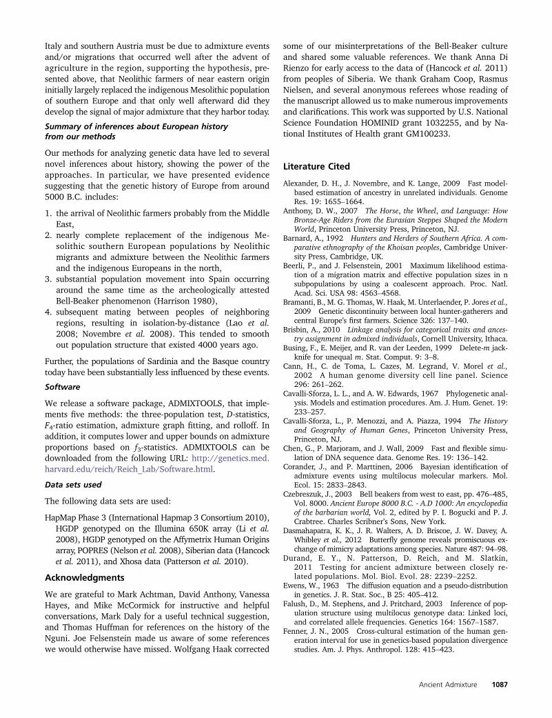
Italy and southern Austria must be due to admixture eventsand/or migrations that occurred well after the advent ofagriculture in the region, supporting the hypothesis, pre-sented above, that Neolithic farmers of near eastern origininitially largely replaced the indigenous Mesolithic populationof southern Europe and that only well afterward did theydevelop the signal of major admixture that they harbor today.

Summary of inferences about European historyfrom our methods

Our methods for analyzing genetic data have led to severalnovel inferences about history, showing the power of theapproaches. In particular, we have presented evidencesuggesting that the genetic history of Europe from around5000 B.C. includes:

1. the arrival of Neolithic farmers probably from the MiddleEast,

2. nearly complete replacement of the indigenous Me-solithic southern European populations by Neolithicmigrants and admixture between the Neolithic farmersand the indigenous Europeans in the north,

3. substantial population movement into Spain occurringaround the same time as the archeologically attestedBell-Beaker phenomenon (Harrison 1980),

4. subsequent mating between peoples of neighboringregions, resulting in isolation-by-distance (Lao et al.2008; Novembre et al. 2008). This tended to smoothout population structure that existed 4000 years ago.

Further, the populations of Sardinia and the Basque countrytoday have been substantially less influenced by these events.

Software

We release a software package, ADMIXTOOLS, that imple-ments five methods: the three-population test, D-statistics,F4-ratio estimation, admixture graph fitting, and rolloff. Inaddition, it computes lower and upper bounds on admixtureproportions based on f3-statistics. ADMIXTOOLS can bedownloaded from the following URL: http://genetics.med.harvard.edu/reich/Reich_Lab/Software.html.

Data sets used

The following data sets are used:

HapMap Phase 3 (International Hapmap 3 Consortium 2010),HGDP genotyped on the Illumina 650K array (Li et al.2008), HGDP genotyped on the Affymetrix Human Originsarray, POPRES (Nelson et al. 2008), Siberian data (Hancocket al. 2011), and Xhosa data (Patterson et al. 2010).

Acknowledgments

We are grateful to Mark Achtman, David Anthony, VanessaHayes, and Mike McCormick for instructive and helpfulconversations, Mark Daly for a useful technical suggestion,and Thomas Huffman for references on the history of theNguni. Joe Felsenstein made us aware of some referenceswe would otherwise have missed. Wolfgang Haak corrected

some of our misinterpretations of the Bell-Beaker cultureand shared some valuable references. We thank Anna DiRienzo for early access to the data of (Hancock et al. 2011)from peoples of Siberia. We thank Graham Coop, RasmusNielsen, and several anonymous referees whose reading ofthe manuscript allowed us to make numerous improvementsand clarifications. This work was supported by U.S. NationalScience Foundation HOMINID grant 1032255, and by Na-tional Institutes of Health grant GM100233.

Literature Cited

Alexander, D. H., J. Novembre, and K. Lange, 2009 Fast model-based estimation of ancestry in unrelated individuals. GenomeRes. 19: 1655–1664.

Anthony, D. W., 2007 The Horse, the Wheel, and Language: HowBronze-Age Riders from the Eurasian Steppes Shaped the ModernWorld, Princeton University Press, Princeton, NJ.

Barnard, A., 1992 Hunters and Herders of Southern Africa. A com-parative ethnography of the Khoisan peoples, Cambridge Univer-sity Press, Cambridge, UK.

Beerli, P., and J. Felsenstein, 2001 Maximum likelihood estima-tion of a migration matrix and effective population sizes in nsubpopulations by using a coalescent approach. Proc. Natl.Acad. Sci. USA 98: 4563–4568.

Bramanti, B., M. G. Thomas, W. Haak, M. Unterlaender, P. Jores et al.,2009 Genetic discontinuity between local hunter-gatherers andcentral Europe’s first farmers. Science 326: 137–140.

Brisbin, A., 2010 Linkage analysis for categorical traits and ances-try assignment in admixed individuals, Cornell University, Ithaca.

Busing, F., E. Meijer, and R. van der Leeden, 1999 Delete-m jack-knife for unequal m. Stat. Comput. 9: 3–8.

Cann, H., C. de Toma, L. Cazes, M. Legrand, V. Morel et al.,2002 A human genome diversity cell line panel. Science296: 261–262.

Cavalli-Sforza, L. L., and A. W. Edwards, 1967 Phylogenetic anal-ysis. Models and estimation procedures. Am. J. Hum. Genet. 19:233–257.

Cavalli-Sforza, L., P. Menozzi, and A. Piazza, 1994 The Historyand Geography of Human Genes, Princeton University Press,Princeton, NJ.

Chen, G., P. Marjoram, and J. Wall, 2009 Fast and flexible simu-lation of DNA sequence data. Genome Res. 19: 136–142.

Corander, J., and P. Marttinen, 2006 Bayesian identification ofadmixture events using multilocus molecular markers. Mol.Ecol. 15: 2833–2843.

Czebreszuk, J., 2003 Bell beakers from west to east, pp. 476–485,Vol. 8000. Ancient Europe 8000 B.C. - A.D 1000: An encyclopediaof the barbarian world, Vol. 2, edited by P. I. Bogucki and P. J.Crabtree. Charles Scribner’s Sons, New York.

Dasmahapatra, K. K., J. R. Walters, A. D. Briscoe, J. W. Davey, A.Whibley et al., 2012 Butterfly genome reveals promiscuous ex-change of mimicry adaptations among species. Nature 487: 94–98.

Durand, E. Y., N. Patterson, D. Reich, and M. Slatkin,2011 Testing for ancient admixture between closely re-lated populations. Mol. Biol. Evol. 28: 2239–2252.

Ewens, W., 1963 The diffusion equation and a pseudo-distributionin genetics. J. R. Stat. Soc., B 25: 405–412.

Falush, D., M. Stephens, and J. Pritchard, 2003 Inference of pop-ulation structure using multilocus genotype data: Linked loci,and correlated allele frequencies. Genetics 164: 1567–1587.

Fenner, J. N., 2005 Cross-cultural estimation of the human gen-eration interval for use in genetics-based population divergencestudies. Am. J. Phys. Anthropol. 128: 415–423.

Ancient Admixture 1087

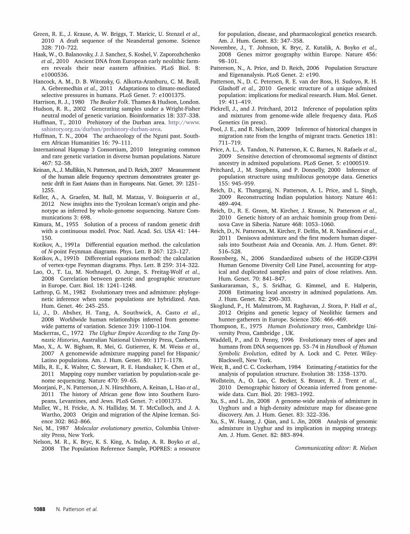
Green, R. E., J. Krause, A. W. Briggs, T. Maricic, U. Stenzel et al.,2010 A draft sequence of the Neandertal genome. Science328: 710–722.

Haak, W., O. Balanovsky, J. J. Sanchez, S. Koshel, V. Zaporozhchenkoet al., 2010 Ancient DNA from European early neolithic farm-ers reveals their near eastern affinities. PLoS Biol. 8:e1000536.

Hancock, A. M., D. B. Witonsky, G. Alkorta-Aranburu, C. M. Beall,A. Gebremedhin et al., 2011 Adaptations to climate-mediatedselective pressures in humans. PLoS Genet. 7: e1001375.

Harrison, R. J., 1980 The Beaker Folk. Thames & Hudson, London.Hudson, R. R., 2002 Generating samples under a Wright-Fisher

neutral model of genetic variation. Bioinformatics 18: 337–338.Huffman, T., 2010 Prehistory of the Durban area. http://www.

sahistory.org.za/durban/prehistory-durban-area.Huffman, T. N., 2004 The archaeology of the Nguni past. South-

ern African Humanities 16: 79–111.International Hapmap 3 Consortium, 2010 Integrating common

and rare genetic variation in diverse human populations. Nature467: 52–58.

Keinan, A., J. Mullikin, N. Patterson, and D. Reich, 2007 Measurementof the human allele frequency spectrum demonstrates greater ge-netic drift in East Asians than in Europeans. Nat. Genet. 39: 1251–1255.

Keller, A., A. Graefen, M. Ball, M. Matzas, V. Boisguerin et al.,2012 New insights into the Tyrolean Iceman’s origin and phe-notype as inferred by whole-genome sequencing. Nature Com-munications 3: 698.

Kimura, M., 1955 Solution of a process of random genetic driftwith a continuous model. Proc. Natl. Acad. Sci. USA 41: 144–150.

Kotikov, A., 1991a Differential equation method. the calculationof N-point Feynman diagrams. Phys. Lett. B 267: 123–127.

Kotikov, A., 1991b Differential equations method: the calculationof vertex-type Feynman diagrams. Phys. Lett. B 259: 314–322.

Lao, O., T. Lu, M. Nothnagel, O. Junge, S. Freitag-Wolf et al.,2008 Correlation between genetic and geographic structurein Europe. Curr. Biol. 18: 1241–1248.

Lathrop, G. M., 1982 Evolutionary trees and admixture: phyloge-netic inference when some populations are hybridized. Ann.Hum. Genet. 46: 245–255.

Li, J., D. Absher, H. Tang, A. Southwick, A. Casto et al.,2008 Worldwide human relationships inferred from genome-wide patterns of variation. Science 319: 1100–1104.

Mackerras, C., 1972 The Uighur Empire According to the Tang Dy-nastic Histories, Australian National University Press, Canberra.

Mao, X., A. W. Bigham, R. Mei, G. Gutierrez, K. M. Weiss et al.,2007 A genomewide admixture mapping panel for Hispanic/Latino populations. Am. J. Hum. Genet. 80: 1171–1178.

Mills, R. E., K. Walter, C. Stewart, R. E. Handsaker, K. Chen et al.,2011 Mapping copy number variation by population-scale ge-nome sequencing. Nature 470: 59–65.

Moorjani, P., N. Patterson, J. N. Hirschhorn, A. Keinan, L. Hao et al.,2011 The history of African gene flow into Southern Euro-peans, Levantines, and Jews. PLoS Genet. 7: e1001373.

Muller, W., H. Fricke, A. N. Halliday, M. T. McCulloch, and J. A.Wartho, 2003 Origin and migration of the Alpine Iceman. Sci-ence 302: 862–866.

Nei, M., 1987 Molecular evolutionary genetics, Columbia Univer-sity Press, New York.

Nelson, M. R., K. Bryc, K. S. King, A. Indap, A. R. Boyko et al.,2008 The Population Reference Sample, POPRES: a resource

for population, disease, and pharmacological genetics research.Am. J. Hum. Genet. 83: 347–358.

Novembre, J., T. Johnson, K. Bryc, Z. Kutalik, A. Boyko et al.,2008 Genes mirror geography within Europe. Nature 456:98–101.

Patterson, N., A. Price, and D. Reich, 2006 Population Structureand Eigenanalysis. PLoS Genet. 2: e190.

Patterson, N., D. C. Petersen, R. E. van der Ross, H. Sudoyo, R. H.Glashoff et al., 2010 Genetic structure of a unique admixedpopulation: implications for medical research. Hum. Mol. Genet.19: 411–419.

Pickrell, J., and J. Pritchard, 2012 Inference of population splitsand mixtures from genome-wide allele frequency data. PLoSGenetics (in press).

Pool, J. E., and R. Nielsen, 2009 Inference of historical changes inmigration rate from the lengths of migrant tracts. Genetics 181:711–719.

Price, A. L., A. Tandon, N. Patterson, K. C. Barnes, N. Rafaels et al.,2009 Sensitive detection of chromosomal segments of distinctancestry in admixed populations. PLoS Genet. 5: e1000519.

Pritchard, J., M. Stephens, and P. Donnelly, 2000 Inference ofpopulation structure using multilocus genotype data. Genetics155: 945–959.

Reich, D., K. Thangaraj, N. Patterson, A. L. Price, and L. Singh,2009 Reconstructing Indian population history. Nature 461:489–494.

Reich, D., R. E. Green, M. Kircher, J. Krause, N. Patterson et al.,2010 Genetic history of an archaic hominin group from Deni-sova Cave in Siberia. Nature 468: 1053–1060.

Reich, D., N. Patterson, M. Kircher, F. Delfin, M. R. Nandineni et al.,2011 Denisova admixture and the first modern human disper-sals into Southeast Asia and Oceania. Am. J. Hum. Genet. 89:516–528.

Rosenberg, N., 2006 Standardized subsets of the HGDP-CEPHHuman Genome Diversity Cell Line Panel, accounting for atyp-ical and duplicated samples and pairs of close relatives. Ann.Hum. Genet. 70: 841–847.

Sankararaman, S., S. Sridhar, G. Kimmel, and E. Halperin,2008 Estimating local ancestry in admixed populations. Am.J. Hum. Genet. 82: 290–303.

Skoglund, P., H. Malmstrom, M. Raghavan, J. Stora, P. Hall et al.,2012 Origins and genetic legacy of Neolithic farmers andhunter-gatherers in Europe. Science 336: 466–469.

Thompson, E., 1975 Human Evolutionary trees, Cambridge Uni-versity Press, Cambridge , UK.

Waddell, P., and D. Penny, 1996 Evolutionary trees of apes andhumans from DNA sequences pp. 53–74 in Handbook of HumanSymbolic Evolution, edited by A. Lock and C. Peter. Wiley-Blackwell, New York.

Weir, B., and C. C. Cockerham, 1984 Estimating f-statistics for theanalysis of population structure. Evolution 38: 1358–1370.

Wollstein, A., O. Lao, C. Becker, S. Brauer, R. J. Trent et al.,2010 Demographic history of Oceania inferred from genome-wide data. Curr. Biol. 20: 1983–1992.

Xu, S., and L. Jin, 2008 A genome-wide analysis of admixture inUyghurs and a high-density admixture map for disease-genediscovery. Am. J. Hum. Genet. 83: 322–336.

Xu, S., W. Huang, J. Qian, and L. Jin, 2008 Analysis of genomicadmixture in Uyghur and its implication in mapping strategy.Am. J. Hum. Genet. 82: 883–894.

Communicating editor: R. Nielsen

1088 N. Patterson et al.

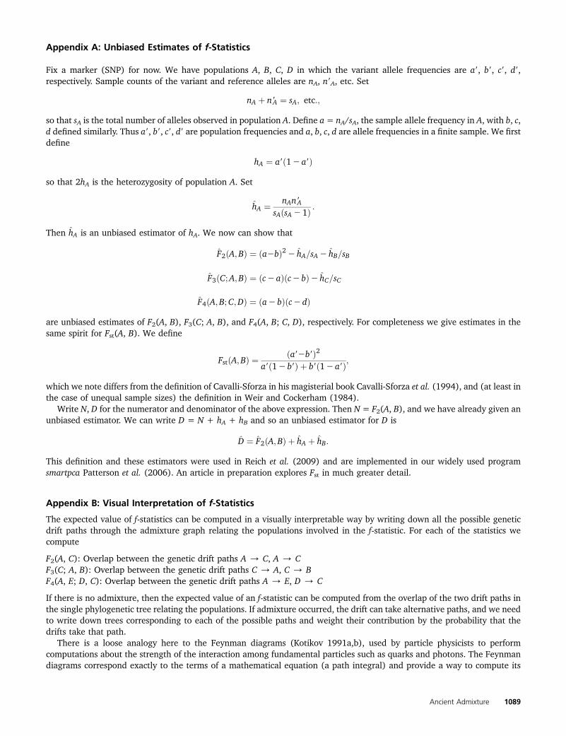
Appendix A: Unbiased Estimates of f-Statistics

Fix a marker (SNP) for now. We have populations A, B, C, D in which the variant allele frequencies are a9, b9, c9, d9,respectively. Sample counts of the variant and reference alleles are nA, n9A, etc. Set

nA þ n9  A ¼ sA; etc:;

so that sA is the total number of alleles observed in population A. Define a= nA/sA, the sample allele frequency in A, with b, c,d defined similarly. Thus a9, b9, c9, d9 are population frequencies and a, b, c, d are allele frequencies in a finite sample. We firstdefine

hA ¼ a9ð12 a9Þ

so that 2hA is the heterozygosity of population A. Set

hA ¼ nAn9  AsAðsA2 1Þ :

Then hA is an unbiased estimator of hA. We now can show that

F2ðA;BÞ ¼ ða2bÞ2 2 hA=sA2 hB=sB

F3ðC;A;BÞ ¼ ðc2 aÞðc2 bÞ2 hC=sC

F4ðA;B;C;DÞ ¼ ða2 bÞðc2 dÞ

are unbiased estimates of F2(A, B), F3(C; A, B), and F4(A, B; C, D), respectively. For completeness we give estimates in thesame spirit for Fst(A, B). We define

FstðA;BÞ ¼ ða92b9Þ2a9ð12 b9Þ þ b9ð12 a9Þ;

which we note differs from the definition of Cavalli-Sforza in his magisterial book Cavalli-Sforza et al. (1994), and (at least inthe case of unequal sample sizes) the definition in Weir and Cockerham (1984).

Write N, D for the numerator and denominator of the above expression. Then N = F2(A, B), and we have already given anunbiased estimator. We can write D = N + hA + hB and so an unbiased estimator for D is

D ¼ F2ðA;BÞ þ hA þ hB:

This definition and these estimators were used in Reich et al. (2009) and are implemented in our widely used programsmartpca Patterson et al. (2006). An article in preparation explores Fst in much greater detail.

Appendix B: Visual Interpretation of f-Statistics

The expected value of f-statistics can be computed in a visually interpretable way by writing down all the possible geneticdrift paths through the admixture graph relating the populations involved in the f-statistic. For each of the statistics wecompute

F2(A, C): Overlap between the genetic drift paths A / C, A / CF3(C; A, B): Overlap between the genetic drift paths C / A, C / BF4(A, E; D, C): Overlap between the genetic drift paths A / E, D / C

If there is no admixture, then the expected value of an f-statistic can be computed from the overlap of the two drift paths inthe single phylogenetic tree relating the populations. If admixture occurred, the drift can take alternative paths, and we needto write down trees corresponding to each of the possible paths and weight their contribution by the probability that thedrifts take that path.

There is a loose analogy here to the Feynman diagrams (Kotikov 1991a,b), used by particle physicists to performcomputations about the strength of the interaction among fundamental particles such as quarks and photons. The Feynmandiagrams correspond exactly to the terms of a mathematical equation (a path integral) and provide a way to compute its

Ancient Admixture 1089

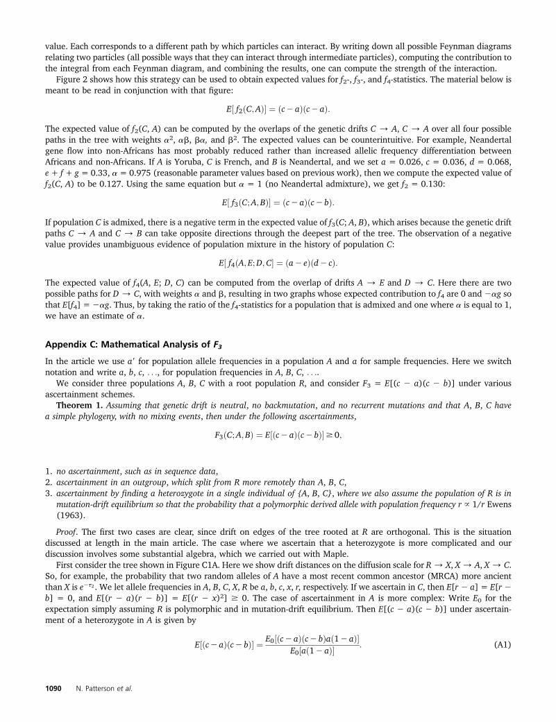
value. Each corresponds to a different path by which particles can interact. By writing down all possible Feynman diagramsrelating two particles (all possible ways that they can interact through intermediate particles), computing the contribution tothe integral from each Feynman diagram, and combining the results, one can compute the strength of the interaction.

Figure 2 shows how this strategy can be used to obtain expected values for f2-, f3-, and f4-statistics. The material below ismeant to be read in conjunction with that figure:

E½ f2ðC;AÞ� ¼ ðc2 aÞðc2 aÞ:

The expected value of f2(C, A) can be computed by the overlaps of the genetic drifts C / A, C / A over all four possiblepaths in the tree with weights a2, ab, ba, and b2. The expected values can be counterintuitive. For example, Neandertalgene flow into non-Africans has most probably reduced rather than increased allelic frequency differentiation betweenAfricans and non-Africans. If A is Yoruba, C is French, and B is Neandertal, and we set a = 0.026, c = 0.036, d = 0.068,e + f + g = 0.33, a = 0.975 (reasonable parameter values based on previous work), then we compute the expected value off2(C, A) to be 0.127. Using the same equation but a = 1 (no Neandertal admixture), we get f2 = 0.130:

E½ f3ðC;A;BÞ� ¼ ðc2 aÞðc2 bÞ:

If population C is admixed, there is a negative term in the expected value of f3(C; A, B), which arises because the genetic driftpaths C / A and C / B can take opposite directions through the deepest part of the tree. The observation of a negativevalue provides unambiguous evidence of population mixture in the history of population C:

E½ f4ðA; E;D;C� ¼ ða2 eÞðd2 cÞ:

The expected value of f4(A, E; D, C) can be computed from the overlap of drifts A / E and D / C. Here there are twopossible paths for D / C, with weights a and b, resulting in two graphs whose expected contribution to f4 are 0 and 2ag sothat E[f4] = 2ag. Thus, by taking the ratio of the f4-statistics for a population that is admixed and one where a is equal to 1,we have an estimate of a.

Appendix C: Mathematical Analysis of F3

In the article we use a9 for population allele frequencies in a population A and a for sample frequencies. Here we switchnotation and write a, b, c, . . ., for population frequencies in A, B, C, . . ..

We consider three populations A, B, C with a root population R, and consider F3 = E[(c 2 a)(c 2 b)] under variousascertainment schemes.

Theorem 1. Assuming that genetic drift is neutral, no backmutation, and no recurrent mutations and that A, B, C havea simple phylogeny, with no mixing events, then under the following ascertainments,

F3ðC;A;BÞ ¼ E½ðc2 aÞðc2 bÞ�$0;

1. no ascertainment, such as in sequence data,2. ascertainment in an outgroup, which split from R more remotely than A, B, C,3. ascertainment by finding a heterozygote in a single individual of {A, B, C}, where we also assume the population of R is in

mutation-drift equilibrium so that the probability that a polymorphic derived allele with population frequency r } 1/r Ewens(1963).

Proof. The first two cases are clear, since drift on edges of the tree rooted at R are orthogonal. This is the situationdiscussed at length in the main article. The case where we ascertain that a heterozygote is more complicated and ourdiscussion involves some substantial algebra, which we carried out with Maple.

First consider the tree shown in Figure C1A. Here we show drift distances on the diffusion scale for R/ X, X/ A, X/ C.So, for example, the probability that two random alleles of A have a most recent common ancestor (MRCA) more ancientthan X is e2t2 . We let allele frequencies in A, B, C, X, R be a, b, c, x, r, respectively. If we ascertain in C, then E[r 2 a] = E[r 2b] = 0, and E[(r 2 a)(r 2 b)] = E[(r 2 x)2] $ 0. The case of ascertainment in A is more complex: Write E0 for theexpectation simply assuming R is polymorphic and in mutation-drift equilibrium. Then E[(c 2 a)(c 2 b)] under ascertain-ment of a heterozygote in A is given by

E½ðc2 aÞðc2 bÞ� ¼ E0½ðc2 aÞðc2 bÞað12 aÞ�E0½að12 aÞ� : (A1)

1090 N. Patterson et al.

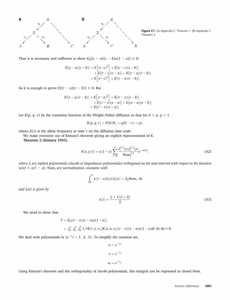
Thus it is necessary and sufficient to show E0[(c 2 a)(c 2 b)a(1 2 a)] $ 0:

E½ðc2 aÞðc2 bÞ� ¼ Ehðr2cÞ2

iþ E½ðr2 cÞðc2 bÞ�

   þ E½ðr2 cÞðc2 aÞ� þ E½ðr2 aÞðr2 bÞ�¼ E

hðr2cÞ2

iþ E½ðr2 aÞðr2 bÞ�:

So it is enough to prove E[(r 2 a)(r 2 b)] $ 0. But

E½ðr2 aÞðr2 bÞ� ¼ Ehðr2xÞ2

iþ E½ðr2 xÞðx2 bÞ�

  þ E½ðr2 xÞðx2 aÞ� þ E½ðx2 aÞðx2 bÞ�¼ E½ðr2 xÞðx2 aÞ�:

Let K(p, q; t) be the transition function of the Wright–Fisher diffusion so that for 0 , p, q , 1

Kðp; q; tÞ ¼ PðXð0Þ ¼ qjXð2tÞ ¼ pÞ;

where X(t) is the allele frequency at time t on the diffusion time scale.We make extensive use of Kimura’s theorem giving an explicit representation of K.Theorem 2 (Kimura 1955).

Kðx; y; tÞ ¼ xð12 xÞXNi¼0

J1;1i ðxÞJ1;1i ðyÞNum1;1

i

e2lðiÞt; (A2)

where Ji are explicit polynomials (Jacobi or Gegenbauer polynomials) orthogonal on the unit interval with respect to the functionw(x) = x(1 2 x). Numi are normalization constants with

Z 1

0xð12 xÞJiðxÞJjðxÞ ¼ dijNumi dx

and l(i) is given by

lðiÞ ¼ ðiþ 1Þðiþ 2Þ2

: (A3)

We need to show that

T ¼ E0½ðr2 xÞðx2 aÞað12 aÞ�

¼ R 10

R 10

R 10 1=rKðr; x; t1ÞKðx; a; t2Þðr2 xÞðx2 aÞað12 aÞdr  dx   da$ 0:

We deal with polynomials in fe2ti i ¼ 1;   2;   3g. To simplify the notation set,

u ¼ e2t1

v ¼ e2t2

w ¼ e2t3 :

Using Kimura’s theorem and the orthogonality of Jacobi polynomials, this integral can be expressed in closed form.

Figure C1 (A) Appendix C, Theorem 1. (B) Appendix C,Theorem 2.

Ancient Admixture 1091

We consider ascertainment of a heterozygote in A. Now calculation shows that

T ¼ vuð12 uÞQ120

;

where Q = 5 + 3v2 + u(5 + 3v2) 2 2v2(u2 + u3 + u4).Noting that 0 # v, u # 1,

Q$ 5þ 3v2 þ u�52 3v2

�$ 0:

Next consider the tree shown in Figure C1B. First suppose we ascertain a heterozygote in A,

E½ðc2 aÞðc2 bÞ� ¼ Ehðc2xÞ2

iþ E½ðx2 aÞðx2 rÞ�

and so we want to show

T ¼ E0½ðx2 aÞðx2 rÞað12 aÞ�$ 0:

A similar calculation to that above shows that

120T ¼ vuð12uÞð12 vÞðvþ 1Þ�2u3 þ 4u2 þ 6uþ 3�$0;

as required. Next suppose we ascertain a heterozygote in C. We now want to show

T ¼ E0½ðc2 xÞðc2 rÞcð12 cÞ�$ 0:

We find

120T ¼ wvð12 vÞQ;

where

Q ¼ 3ð1þ vÞ þ 5u2ð1þ vÞ2 2u5v2�1þ vþ v2

�:

We need to show Q$ 0. Expanding Q into monomials with coefficients61 there are six negative terms, each of which can bepaired with a positive term of lower degree.

This completes the proof.Summarizing, our three-population test is rigorous if there is ascertainment in an outgroup only (or no ascertainment as

in sequence data). It also is rigorous with a variety of other simple ascertainments. Further in practice, on commercial SNParrays, highly significant false positives do not seem to arise as we show in Table 5.

Appendix D: Simulations to Test f-Statistic Methodology

To test the robustness of our f-statistic methodology, we carried out coalescent simulations of five populations relatedaccording to Figure 4, using ms (Hudson 2002).

Our simulations involved specifying six dates:

1. tadmix: Date of admixture between populations B9 and C9.2. tBB9: Date of divergence of populations B and B9.3. tCC9: Date of divergence of populations C and C9.4. tABB9: Date of divergence of population A from the B, B9 clade.5. tABB9CC9: Date of divergence of the A, B, B9 and C, C9 clades.6. tO: Date of divergence of the A, B, B9, C, C9 clade and the outgroup O.

We assumed that all populations were constant in size in the periods between when they split, with the following diploidsizes:

1. Nx: Size in the ancestry of population X.2. NB9: Size in the ancestry of population B9’.3. NB: Size in the ancestry of population B.

1092 N. Patterson et al.

4. NC9: Size in the ancestry of population C9.5. NC: Size in the ancestry of population C.6. NO: Size in the recent ancestry of the outgroup O.7. NBB9: Size in the common ancestry of B and B9.8. NCC9: Size in the common ancestry of C and C9.9. NABB9: Size in the common ancestry of A, B, and B9.

10. NABB9CC9: Size in the common ancestry of A, B, B9, C, and C9.11. NABB9CC9O: Size in the common ancestry of all populations.

We picked population sizes, times, and Fst to approximately match empirical data for

A: Adygei, West EurasianB: French, West EurasianC: Han, East AsianX: Uygur, AdmixedY: Yoruba, Outgroup

Thus, our baseline simulations correspond to a roughly plausible scenario for some of the genetic history of Eurasia, withYoruba serving as an outgroup. We then varied parameters, as well as ascertainments of SNPs, and explored how thisaffected the observed values from simulation.

In Table 1 we show baseline demographic parameters, as well as several alternatives that each involved varying a singleparameter compared with the baseline. Each alternate parameter set was separately assessed by simulation (includingdifferent SNP ascertainments).

Table 1 shows the results. We find that:

• Fst-statistics change as expected depending on SNP ascertainment and demographic history.• The consistency of D-statistics with 0 in the absence of admixture is robust to SNP ascertainment. Substantially nonzero

values are observed only when the test population is admixed (X) and not when it is unadmixed (B).• f3-statistics are negative when the test population is admixed (X) except for high population-specific drift, which masks the

signal as expected. Statistics are always positive when the test population is unadmixed (B), regardless of ascertainment.

Thus, these simulations show that inferences about history based on the f-statistics are robust to ascertainment process as weargued in the main text on theoretical grounds.

Ancient Admixture 1093

GENETICSSupporting Information

http://www.genetics.org/lookup/suppl/doi:10.1534/genetics.112.145037/-/DC1

Ancient Admixture in Human HistoryNick Patterson, Priya Moorjani, Yontao Luo, Swapan Mallick, Nadin Rohland, Yiping Zhan,

Teri Genschoreck, Teresa Webster, and David Reich

Copyright © 2012 by the Genetics Society of AmericaDOI: 10.1534/genetics.112.145037

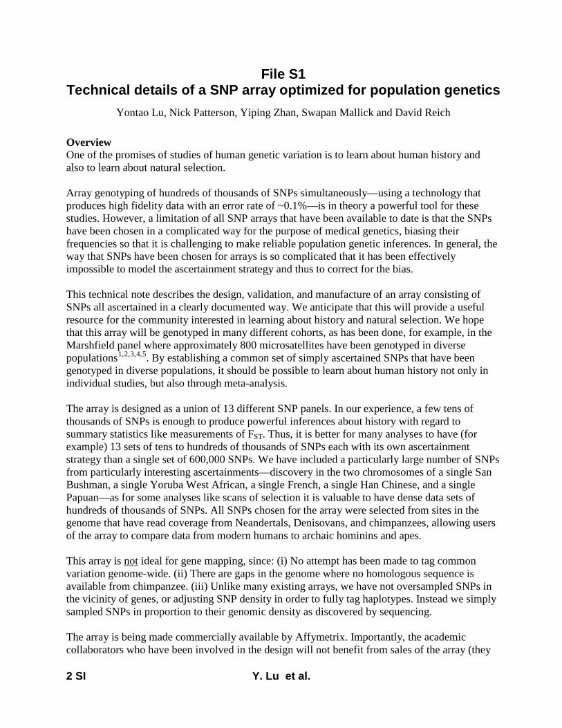
2 SI Y. Lu et al.

File S1 Technical details of a SNP array optimized for population genetics

Yontao Lu, Nick Patterson, Yiping Zhan, Swapan Mallick and David Reich

Overview One of the promises of studies of human genetic variation is to learn about human history and also to learn about natural selection. Array genotyping of hundreds of thousands of SNPs simultaneously—using a technology that produces high fidelity data with an error rate of ~0.1%—is in theory a powerful tool for these studies. However, a limitation of all SNP arrays that have been available to date is that the SNPs have been chosen in a complicated way for the purpose of medical genetics, biasing their frequencies so that it is challenging to make reliable population genetic inferences. In general, the way that SNPs have been chosen for arrays is so complicated that it has been effectively impossible to model the ascertainment strategy and thus to correct for the bias. This technical note describes the design, validation, and manufacture of an array consisting of SNPs all ascertained in a clearly documented way. We anticipate that this will provide a useful resource for the community interested in learning about history and natural selection. We hope that this array will be genotyped in many different cohorts, as has been done, for example, in the Marshfield panel where approximately 800 microsatellites have been genotyped in diverse populations1,2,3,4,5. By establishing a common set of simply ascertained SNPs that have been genotyped in diverse populations, it should be possible to learn about human history not only in individual studies, but also through meta-analysis. The array is designed as a union of 13 different SNP panels. In our experience, a few tens of thousands of SNPs is enough to produce powerful inferences about history with regard to summary statistics like measurements of FST. Thus, it is better for many analyses to have (for example) 13 sets of tens to hundreds of thousands of SNPs each with its own ascertainment strategy than a single set of 600,000 SNPs. We have included a particularly large number of SNPs from particularly interesting ascertainments—discovery in the two chromosomes of a single San Bushman, a single Yoruba West African, a single French, a single Han Chinese, and a single Papuan—as for some analyses like scans of selection it is valuable to have dense data sets of hundreds of thousands of SNPs. All SNPs chosen for the array were selected from sites in the genome that have read coverage from Neandertals, Denisovans, and chimpanzees, allowing users of the array to compare data from modern humans to archaic hominins and apes. This array is not ideal for gene mapping, since: (i) No attempt has been made to tag common variation genome-wide. (ii) There are gaps in the genome where no homologous sequence is available from chimpanzee. (iii) Unlike many existing arrays, we have not oversampled SNPs in the vicinity of genes, or adjusting SNP density in order to fully tag haplotypes. Instead we simply sampled SNPs in proportion to their genomic density as discovered by sequencing. The array is being made commercially available by Affymetrix. Importantly, the academic collaborators who have been involved in the design will not benefit from sales of the array (they

3 SI Y. Lu et al.

will not receive any financial compensation from Affymetrix). The CEPH-Human Genome Diversity Project (CEPH-HGDP) samples that were genotyped during the course of the project will not be used for any commercial purposes. Affymetrix deposited the genotypes of unrelated CEPH-HGDP samples, collected as part of the array development, into the CEPH-HGDP database on August 12, 2011, more than six months before commercial release of the array (in Spring 2012), and this genotyping data is freely available to the public. Design strategy for the 13 panels (Panels 1-12) Discovery of heterozygous sites within 12 individuals of known ancestry The first 12 SNP ascertainment strategies are based on the idea of the Keinan, Mullikin et al. Nature Genetics 2007 paper6. That paper takes advantage of the fact that by discovering SNPs in a comparison of two chromosomes from the same individual of known ancestry, and then genotyping in a larger panel of samples from the same population, one can learn about history in a way that is not affected by the frequency of the SNP in human populations. In particular, even though we may miss a substantial proportion of real SNPs in the individual (false-negatives), and even if a substantial proportion of discovered SNP are false-positives, we expect that the inferences about history using SNPs discovered in this way will be as accurate as what would be obtained using SNPs identified from deep sequencing with perfect readout of alleles. To understand why false-negative SNPs should not bias inferences, we note that if a SNP is truly heterozygous in the individual in whom we are trying to discover it, there is exactly one copy of the ancestral allele and exactly one copy of the derived allele. Thus, conditional on the SNP being heterozygous in the discovery individual, its probability of being discovered is not further affected by whether it has a high or low minor allele frequency in the population. This contrasts with ascertainment strategies that discover SNPs in more than one individual, where there is always a real (and extremely difficult to quantify) bias toward missing rarer variants. By genotyping SNPs discovered in this way, and making a simple p(1-p) correction for discovery in two chromosomes (where p is the minor allele frequency), one can obtain an unbiased reconstruction of the allele frequency distribution in the population. An important feature of this SNP discovery strategy is that false-positive SNPs (for example, due to sequencing error, mapping error, segmental duplications or copy number variation) are not expected to substantially bias inferences. The reason is that we have validated all candidate SNPs by genotyping them using a different technology, and we have required the genotypes to match the individuals in whom they were discovered. Thus, we expect to have a negligible proportion of false-positive SNPs on the final array. This procedure has produced 12 panels of uniformly discovered SNPs, which can be used for allele frequency spectrum analysis. There is some overlap of SNPs across panels. Importantly, we have separately determined validation status for the SNPs in each panel, and have only used SNPs that validate in the same sample in which they were discovered. Thus, we have not biased toward SNPs with a high minor allele frequency, or that are polymorphic across multiple populations, which might be expected to have a higher chance of validation if we did not perform the validation in each discovery sample independently.

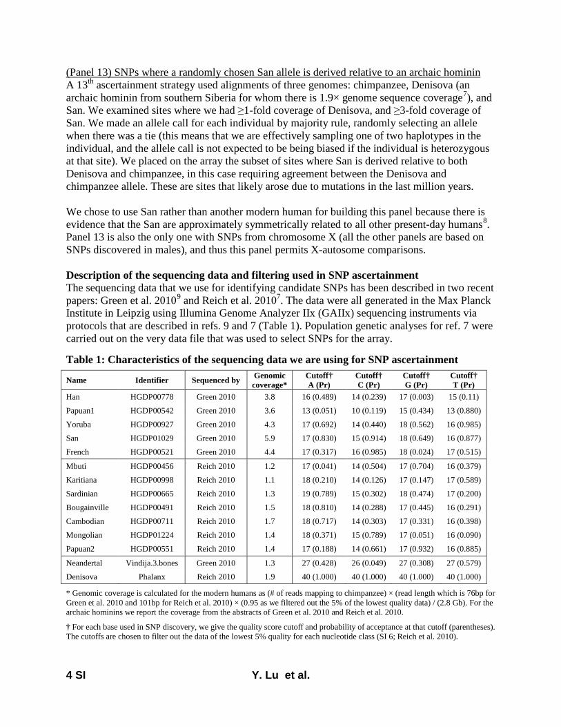
4 SI Y. Lu et al.

(Panel 13) SNPs where a randomly chosen San allele is derived relative to an archaic hominin A 13th ascertainment strategy used alignments of three genomes: chimpanzee, Denisova (an archaic hominin from southern Siberia for whom there is 1.9× genome sequence coverage7), and San. We examined sites where we had ≥1-fold coverage of Denisova, and ≥3-fold coverage of San. We made an allele call for each individual by majority rule, randomly selecting an allele when there was a tie (this means that we are effectively sampling one of two haplotypes in the individual, and the allele call is not expected to be being biased if the individual is heterozygous at that site). We placed on the array the subset of sites where San is derived relative to both Denisova and chimpanzee, in this case requiring agreement between the Denisova and chimpanzee allele. These are sites that likely arose due to mutations in the last million years. We chose to use San rather than another modern human for building this panel because there is evidence that the San are approximately symmetrically related to all other present-day humans8. Panel 13 is also the only one with SNPs from chromosome X (all the other panels are based on SNPs discovered in males), and thus this panel permits X-autosome comparisons. Description of the sequencing data and filtering used in SNP ascertainment The sequencing data that we use for identifying candidate SNPs has been described in two recent papers: Green et al. 20109 and Reich et al. 20107. The data were all generated in the Max Planck Institute in Leipzig using Illumina Genome Analyzer IIx (GAIIx) sequencing instruments via protocols that are described in refs. 9 and 7 (Table 1). Population genetic analyses for ref. 7 were carried out on the very data file that was used to select SNPs for the array. Table 1: Characteristics of the sequencing data we are using for SNP ascertainment

Name Identifier Sequenced by Genomic coverage*

Cutoff† A (Pr)

Cutoff† C (Pr)

Cutoff† G (Pr)

Cutoff† T (Pr)

Han HGDP00778 Green 2010 3.8 16 (0.489) 14 (0.239) 17 (0.003) 15 (0.11)

Papuan1 HGDP00542 Green 2010 3.6 13 (0.051) 10 (0.119) 15 (0.434) 13 (0.880)

Yoruba HGDP00927 Green 2010 4.3 17 (0.692) 14 (0.440) 18 (0.562) 16 (0.985)

San HGDP01029 Green 2010 5.9 17 (0.830) 15 (0.914) 18 (0.649) 16 (0.877)

French HGDP00521 Green 2010 4.4 17 (0.317) 16 (0.985) 18 (0.024) 17 (0.515)

Mbuti HGDP00456 Reich 2010 1.2 17 (0.041) 14 (0.504) 17 (0.704) 16 (0.379)

Karitiana HGDP00998 Reich 2010 1.1 18 (0.210) 14 (0.126) 17 (0.147) 17 (0.589)

Sardinian HGDP00665 Reich 2010 1.3 19 (0.789) 15 (0.302) 18 (0.474) 17 (0.200)

Bougainville HGDP00491 Reich 2010 1.5 18 (0.810) 14 (0.288) 17 (0.445) 16 (0.291)

Cambodian HGDP00711 Reich 2010 1.7 18 (0.717) 14 (0.303) 17 (0.331) 16 (0.398)

Mongolian HGDP01224 Reich 2010 1.4 18 (0.371) 15 (0.789) 17 (0.051) 16 (0.090)

Papuan2 HGDP00551 Reich 2010 1.4 17 (0.188) 14 (0.661) 17 (0.932) 16 (0.885)

Neandertal Vindija.3.bones Green 2010 1.3 27 (0.428) 26 (0.049) 27 (0.308) 27 (0.579)

Denisova Phalanx Reich 2010 1.9 40 (1.000) 40 (1.000) 40 (1.000) 40 (1.000)

* Genomic coverage is calculated for the modern humans as (# of reads mapping to chimpanzee) × (read length which is 76bp for Green et al. 2010 and 101bp for Reich et al. 2010) × (0.95 as we filtered out the 5% of the lowest quality data) / (2.8 Gb). For the archaic hominins we report the coverage from the abstracts of Green et al. 2010 and Reich et al. 2010.

† For each base used in SNP discovery, we give the quality score cutoff and probability of acceptance at that cutoff (parentheses). The cutoffs are chosen to filter out the data of the lowest 5% quality for each nucleotide class (SI 6; Reich et al. 2010).

5 SI Y. Lu et al.

The 12 modern human samples are all from the CEPH-HGDP panel. A valuable feature of this panel is that DNA for all samples is available on request on a cost-recovery basis for researchers who wish to carry out further sequencing and genotyping analysis on these samples for the purpose of research into human population history8,10. Five of the samples (San, Yoruba, Han, French and a Papuan) were sequenced by Green et al. 2010 using Illumina paired-end 76bp reads9, while the remaining 7 (Mbuti, Sardinian, Karitiana, Mongolian, Cambodian, Bougainville, and a second Papuan) were sequenced by Reich et al. 2010 using Illumina paired-end 101bp reads7. All reads from all 12 samples were mapped to chimpanzee (PanTro2). To filter the sequence data for analysis, we used a similar procedure as described in Reich et al. 20107, removing the lowest quality of 5% of nucleotides on a sample and nucleotide-specific basis to maximize the amount of sequencing data available for analysis. After this procedure, we had 3.6-5.9× coverage for the 5 samples and 1.1-1.7× for the 7 samples (Table 1). We also used data from 4 ancient DNA samples to aid our choice of SNPs. To represent Neandertals, we used a pool of sequences from 3 bones from Vindija Cave in Croatia (Vi33.16, Vi33.25 and Vi33.26) for which we had 1.3× genome coverage altogether9. To represent Denisovans, we used data from a finger bone (fifth distal manual phalanx) from the Altai mountains of southern Siberia, with 1.9× coverage7. All reads are mapped to chimpanzee and a chimpanzee allele is available We mapped sequencing reads from modern and ancient genomes to the chimpanzee reference sequence (PanTro2) to avoid biases toward one present-day human group more than another. We filtered out reads with a substantial probability of poor mapping Each read that we analyzed had a mapping quality score (MAPQ) that reflects the confidence of its mapping to PanTro2. Based on empirical exploration of the usefulness of the scores, which were generated by either the ANFO or BWA software, we only used reads that had MAPQ of at least 90 for Neandertal (ANFO mapping), 37 for Denisova (BWA), and 60 for present-day humans (BWA). We also rejected reads if the alignment to the chimpanzee resulted in any insertion/deletion difference. This filter was applied in addition to the filtering of Table 1. Filtering of sites with ≥2 alleles not matching chimp across the humans used for SNP discovery. At a small proportion of sites, we observe more than one non-ancestral allele in the individual sequencing data used for SNP discovery. Such sites cannot be due to a single historical mutation. Instead, the data must reflect at least two mutations or sequencing errors. We filter out such sites. For a very small fraction of sites, we found that the derived allele is different depending on which human is used in SNP discovery (these are potentially triallelic SNPs in the population, although they are not triallelic in the discovery individual). We keep such sites in our list of SNPs for designing, and use multiple probe sets to assay such SNPs.

The raw data file that emerges from this process is available on the “orchestra” Harvard Medical School filesystem at: /groups/reich/CLEAN_SNP_ARRAY/rawsnps and is freely available from David Reich on request (a README file is in the same directory at rawsnps_readme) (Table 2). For brevity, this file only lists the 2,173,116 SNPs where 2 copies of the derived and 1 copy of the ancestral allele are observed a hominin; these are the only SNPs that are candidates for inclusion. Thus, it is an abbreviated version of a larger file used in analyses for ref. 7.

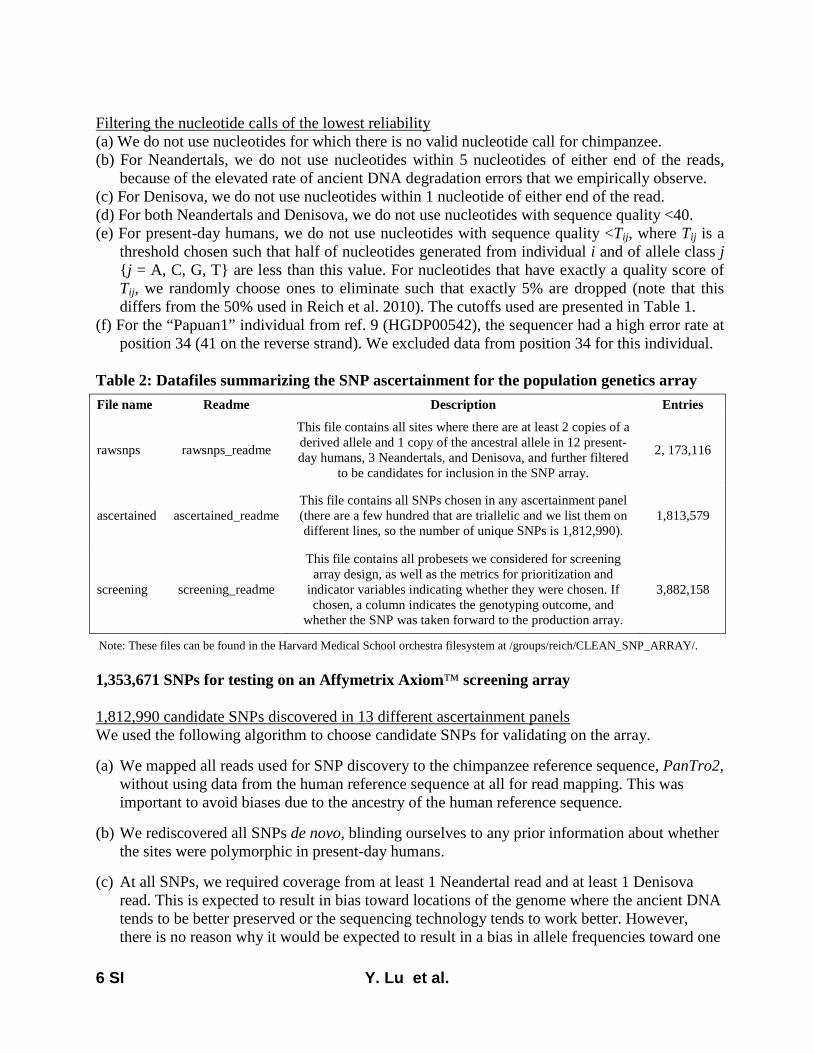
6 SI Y. Lu et al.

Filtering the nucleotide calls of the lowest reliability (a) We do not use nucleotides for which there is no valid nucleotide call for chimpanzee. (b) For Neandertals, we do not use nucleotides within 5 nucleotides of either end of the reads,

because of the elevated rate of ancient DNA degradation errors that we empirically observe. (c) For Denisova, we do not use nucleotides within 1 nucleotide of either end of the read. (d) For both Neandertals and Denisova, we do not use nucleotides with sequence quality <40. (e) For present-day humans, we do not use nucleotides with sequence quality <Tij, where Tij is a

threshold chosen such that half of nucleotides generated from individual i and of allele class j {j = A, C, G, T} are less than this value. For nucleotides that have exactly a quality score of Tij, we randomly choose ones to eliminate such that exactly 5% are dropped (note that this differs from the 50% used in Reich et al. 2010). The cutoffs used are presented in Table 1.

(f) For the “Papuan1” individual from ref. 9 (HGDP00542), the sequencer had a high error rate at position 34 (41 on the reverse strand). We excluded data from position 34 for this individual.

Table 2: Datafiles summarizing the SNP ascertainment for the population genetics array

File name Readme Description Entries

rawsnps rawsnps_readme

This file contains all sites where there are at least 2 copies of a derived allele and 1 copy of the ancestral allele in 12 present-day humans, 3 Neandertals, and Denisova, and further filtered

to be candidates for inclusion in the SNP array.

2, 173,116

ascertained ascertained_readme This file contains all SNPs chosen in any ascertainment panel (there are a few hundred that are triallelic and we list them on different lines, so the number of unique SNPs is 1,812,990).

1,813,579

screening screening_readme

This file contains all probesets we considered for screening array design, as well as the metrics for prioritization and

indicator variables indicating whether they were chosen. If chosen, a column indicates the genotyping outcome, and

whether the SNP was taken forward to the production array.

3,882,158

Note: These files can be found in the Harvard Medical School orchestra filesystem at /groups/reich/CLEAN_SNP_ARRAY/. 1,353,671 SNPs for testing on an Affymetrix Axiom™ screening array 1,812,990 candidate SNPs discovered in 13 different ascertainment panels We used the following algorithm to choose candidate SNPs for validating on the array. (a) We mapped all reads used for SNP discovery to the chimpanzee reference sequence, PanTro2,

without using data from the human reference sequence at all for read mapping. This was important to avoid biases due to the ancestry of the human reference sequence.

(b) We rediscovered all SNPs de novo, blinding ourselves to any prior information about whether

the sites were polymorphic in present-day humans.

(c) At all SNPs, we required coverage from at least 1 Neandertal read and at least 1 Denisova read. This is expected to result in bias toward locations of the genome where the ancient DNA tends to be better preserved or the sequencing technology tends to work better. However, there is no reason why it would be expected to result in a bias in allele frequencies toward one

7 SI Y. Lu et al.

modern human population more than another (as all Neandertal and Denisova reads are mapped to chimpanzee, and no modern human data influences the mapping). The availability of data from archaic hominins from each of the SNPs on our array should be of value for some types of population genetic analysis. (For a handful of sites, the Denisova and Neandertal alleles may not be the same as those seen in present-day humans, but we nevertheless considered these sites to be covered by Denisova and Neandertal as we were concerned that not doing so could introduce bias. Users can treat such sites how they wish.)

(d) All A/T and C/G polymorphisms were excluded, since genotyping these SNPs requires twice

the number of probes using the Axiom™ technology. Thus, removing them increases the number of SNPs we can include on a single array. Removing these SNPs has the additional benefit that it eliminates any strand ambiguity. (Illumina arrays do not genotype A/T or C/G SNPs, either.) However, it also had the disadvantage that A/T and C/G SNPS constitute the one class of SNPs that is believed to be immune to biased gene conversion. Thus, in population genetic analyses of the data generated from the array, it will be important to assess whether inferences are potentially explained by biased gene conversion.

(e) For the SNPs for panels 1-12 (candidate heterozygotes in an individual of known ancestry),

we required the observation of at least 2 copies of the derived (non-chimpanzee) and at least 1 copy of the ancestral allele in the studied person (Reich et al. 2010; SI 6). We did not include chromosome X SNPs from these panels as the 12 individuals were all male.

(f) For the SNPs in panel 13 (derived in San relative to Denisova), we restricted to sites where we

had ≥3-fold read coverage of San and ≥1-fold read coverage of Denisova. A complication in choosing SNPs discovered in two individuals is that both the San and

Denisova individuals are diploid. What we want is to have a panel of SNPs ascertained by comparing a single haploid Denisovan and a single haploid San chromosome, but if we are not careful, we are going to be biased toward the SNPs that are fixed differences. For example, if we accepted only SNPs where all Denisova reads matched chimpanzee and all San reads were derived, then we would bias against SNPs that were truly heterozygous.

To obtain data of the type that would be expected from sampling a single haploid Denisovan and a single haploid San chromosome, we picked the allele that was seen more often in each sample to represent that sample (if there was a tie in terms of the number of reads supporting each allele, we chose one allele at random). In this way, we are picking one of the two chromosomes from each individual (at random), and hence we are effectively sampling a haploid chromosome despite having diploid data. An additional benefit of using the majority rule is that we are also increasing the quality and reliability of the allele call, such that we expect a larger proportion of these SNPs to be real than in panels 1-12.

From the SNPs discovered in this way, we restrict our analysis to sites where Denisova matches the chimpanzee allele and where San is derived (we throw away sites where San is ancestral and Denisova is derived). The reason for this is that this is the only subset of SNPs that we can experimentally validate. To validate these SNPs, we can genotype the San individual and require the observation of an allele that differs from chimpanzee. In contrast, we cannot validate sites where San is ancestral and Denisova is derived, since the Denisova sample is extremely limited and does not provide enough for genotyping assays.

Some of the SNPs from panels 1-13 overlap. Thus, while the sum of the number of SNPs in each panel is 2,581,282, the number of unique SNPs is only 1,812,990. However, the fact that a SNP is

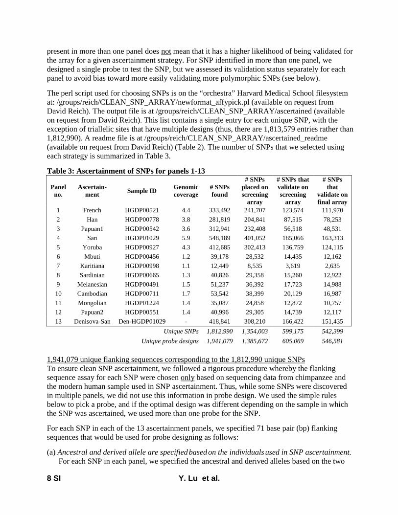
8 SI Y. Lu et al.

present in more than one panel does not mean that it has a higher likelihood of being validated for the array for a given ascertainment strategy. For SNP identified in more than one panel, we designed a single probe to test the SNP, but we assessed its validation status separately for each panel to avoid bias toward more easily validating more polymorphic SNPs (see below). The perl script used for choosing SNPs is on the “orchestra” Harvard Medical School filesystem at: /groups/reich/CLEAN_SNP_ARRAY/newformat_affypick.pl (available on request from David Reich). The output file is at /groups/reich/CLEAN_SNP_ARRAY/ascertained (available on request from David Reich). This list contains a single entry for each unique SNP, with the exception of triallelic sites that have multiple designs (thus, there are 1,813,579 entries rather than 1,812,990). A readme file is at /groups/reich/CLEAN_SNP_ARRAY/ascertained_readme (available on request from David Reich) (Table 2). The number of SNPs that we selected using each strategy is summarized in Table 3. Table 3: Ascertainment of SNPs for panels 1-13

Panel no.

Ascertain-ment Sample ID Genomic

coverage # SNPs found

# SNPs placed on screening

array

# SNPs that validate on screening

array

# SNPs that

validate on final array

1 French HGDP00521 4.4 333,492 241,707 123,574 111,970 2 Han HGDP00778 3.8 281,819 204,841 87,515 78,253 3 Papuan1 HGDP00542 3.6 312,941 232,408 56,518 48,531 4 San HGDP01029 5.9 548,189 401,052 185,066 163,313 5 Yoruba HGDP00927 4.3 412,685 302,413 136,759 124,115 6 Mbuti HGDP00456 1.2 39,178 28,532 14,435 12,162 7 Karitiana HGDP00998 1.1 12,449 8,535 3,619 2,635 8 Sardinian HGDP00665 1.3 40,826 29,358 15,260 12,922 9 Melanesian HGDP00491 1.5 51,237 36,392 17,723 14,988 10 Cambodian HGDP00711 1.7 53,542 38,399 20,129 16,987 11 Mongolian HGDP01224 1.4 35,087 24,858 12,872 10,757 12 Papuan2 HGDP00551 1.4 40,996 29,305 14,739 12,117 13 Denisova-San Den-HGDP01029 - 418,841 308,210 166,422 151,435

Unique SNPs 1,812,990 1,354,003 599,175 542,399

Unique probe designs 1,941,079 1,385,672 605,069 546,581 1,941,079 unique flanking sequences corresponding to the 1,812,990 unique SNPs To ensure clean SNP ascertainment, we followed a rigorous procedure whereby the flanking sequence assay for each SNP were chosen only based on sequencing data from chimpanzee and the modern human sample used in SNP ascertainment. Thus, while some SNPs were discovered in multiple panels, we did not use this information in probe design. We used the simple rules below to pick a probe, and if the optimal design was different depending on the sample in which the SNP was ascertained, we used more than one probe for the SNP. For each SNP in each of the 13 ascertainment panels, we specified 71 base pair (bp) flanking sequences that would be used for probe designing as follows: (a) Ancestral and derived allele are specified based on the individuals used in SNP ascertainment.

For each SNP in each panel, we specified the ancestral and derived alleles based on the two

9 SI Y. Lu et al.

alleles observed in SNP ascertainment, defining as “ancestral” the allele that matched chimpanzee. SNPs within any ascertainment panel almost always had two observed alleles, since we filtered out sites with three or more. However, for SNPs that were discovered in multiple panels, we performed the specification of the ancestral and derived allele independently, and thus for a small fraction of sites, there was a different derived allele depending on the ascertainment panel (even if flanking sequence were sometimes identical).

(b) Flanking sequence is specified entirely based on the modern sample used for SNP discovery.

For initial probe design, we provided 35 bp of flanking sequence on either side of the SNP. We started with 71 bp of sequence from the chimpanzee genome, PanTro2, centered on the SNP. To decrease the number of mismatches between the flanking sequence and any human that might be analyzed using the array, we “humanized” the flanking sequence based on the modern sample used for SNP discovery (importantly, only the discovery sample is used for the humanization of the sequence, and so the ancestry of other samples cannot bias results).

Specifically, for each of panels 1-13, we took all reads from the modern human used in SNP ascertainment that mapped to the flanking nucleotide. Where 100% of reads disagreed with PanTro2, we edited the flanking sequence to reflect that in the ascertainment sample. Otherwise, we kept the chimpanzee allele. An example is: “acctggctccagGgccagcagctccgtcaAggtcc[G/A]ctgcatgaaactgatgaaggggagggcaccaggcg”. Here, capital [G/A] indicates the [chimp/alternate allele] at the SNP and other capital letters indicate bases edited from the chimpanzee reference to match the ascertainment sample. For ascertainment panel 13 (Denisova ancestral and a randomly chosen San allele derived), we did not use the Denisova genome in primer editing. Instead, we edited the sequence to match San whenever San consistently had a non-chimpanzee allele at all reads overlapping the site.

Because the steps above sometimes result in different flanking sequences for the same nucleotide (depending on the particular sequencing reads from the sample used in SNP ascertainment), we were left with more unique flanking sequences (n=1,941,079) than unique SNPs (n=1,812,991).

Procedure used to choose 1,385,671 oligonucleotide probes for the screening array With the list of 1,951,079 flanking sequences, we needed to design oligonucleotide probes, or “probesets”, for a screening array. We blinded ourselves to prior knowledge about which probes worked in previous assays using the Axiom™ technology, since doing so would expected to lead to a higher validation success rate for probes that have been previously tried on SNP arrays (introducing complex biases). For the same reason, we did not modify probe design based on using information in databases about polymorphism in flanking sequence. The only two types of information that were used in probe design were the physical chemistry considerations of which probes are expected to work well, and mapping information to the PanTro2 chimp genome. All the metrics used are in a file on the “orchestra” Harvard Medical School filesystem /groups/reich/CLEAN_SNP_ARRAY/probesets, available on request from David Reich (Table 2). Details of the filtering procedure that we applied are as follows:

(a) We first identified 3,882,158 candidate probesets (two 30mers for each flanking sequence)

For each of the 1,941,079 flanking sequences, it is possible to design two probesets corresponding to the 30 bp 5’ or 3’ direction of the SNP. We use the shorthand “red” to designate the 5’ probe and “green” to designate the 3’ probe, always referenced relative to the positive strand of the chimpanzee genome sequence PanTro2 (Figure 1).

10 SI Y. Lu et al.

(b) We next restricted analysis to 2,294,760 probesets predicted to have greater success Of the 3,882,158 candidate probesets (2 for each of 1,941,079 flanking sequences), we computed metrics that based on past experience were useful for predicting the success of genotyping. The values of the metrics are in /groups/reich/CLEAN_SNP_ARRAY/probesets (see probesets_readme), available on request from David Reich. We applied the following filters to winnow the list to 2,294,760:

(i) Removing probesets that map to multiple positions in chimpanzee. (ii) Best BLAT hit to PanTro2 is much better than the second-best hit. We used BLAT to map

each 35 bp flanking sequence to PanTro2. We required a minimum of 33 bp of alignment, and required the difference between the first and second hits to be >5.

(iii) 16mers within the probeset are relatively unique. For each candidate 30 bp probeset, we examined each unique 16mer in a sliding window along the sequence (15 in all), and counted the number of exact matches in PanTro2. We defined “16mer-max” as the maximum number of exact matches seen for any of these 16-mers. In the experience of Affymetrix scientists who have worked on the Axiom™ technology, non-specific binding is unlikely when 16mer-max is small. We required “16mer-max” <110.

(iv) No runs of 4 G’s. When more than 4 consecutive Gs stack up into quartets, hybridization tends to be compromised. We filtered out probes that had runs of 4 G’s (or 4 C’s),

(v) Terminal 5mer is not complemented elsewhere in the probeset. We required the 5’ terminal 5mer to not have a reverse complement elsewhere in the probeset sequence, to minimize the tendency toward inter/intra probe annealing during hybridization, which in previous experience with the Axiom™ technology could cause a lower success rate.

(vi) Number of G and C nucleotides is >5. We required that >5 of the nucleotides were either G or C. Previous experience suggests that probesets with extremely low G or C usually do not work well for hybridization assays.

(c) A list of 1,477,155 probesets after eliminating redundancy For flanking sequences where both candidate probesets passed the filters above, we chose the probeset that was deemed more likely to succeed based on having a lower value of “16mer-max” metric. When both probesets had the same value of “16mer-max”, we used a random number generator to choose. This resulted in 1,525,604 candidate probesets.

Even after representing each flanking sequence by no more than one probeset, the resulting list contained 48,449 duplicative entries. This occurred when the same SNP (and probeset) had been independently selected in more than one of the 13 ascertainment panels. In such cases, the 71bp flanking sequence obtained as described above could be distinct for multiple SNP ascertainments, but sub-strings could be identical, so that it could happen that the 30mer that was selected to represent the SNP was identical. We therefore merged these probes to eliminate redundancy, leaving us with 1,477,155 unique probesets.

11 SI Y. Lu et al.

Our naming scheme for probesets contains a binary string of 13 characters providing the ascertainment information for that probe. Because we merged some probesets, we created a new ascertainment code called “asc.new”. This was generated by applying a bitwise-or operation to the binary strings of 13 characters corresponding to the ascertainment information for the redundant probes.

(d) A final list of 1,385,672 probes that were placed on the screening array

The 1,477,155 probes that passed our filters were more than could fit into the screening array. Thus, we ranked all the probes based on their “16mer-max” score, breaking ties using a random number generator (lower values have a higher rank). After this ranking, all probes had “16mer-max” of no more than 110, and we were left with 1,385,672 probes.

Design, genotyping, and analysis of screening array Design of the screening array We designed two arrays to screen these 1.39 million probesets (0.69 million probesets fit onto a single screening array). To minimize bias, we randomized the probes with respect to which one of the 2 screening arrays was used to test them. We also used standard chip design strategies that are applied at Affymetrix for determining probe location in each screen design. The number of SNPs from each panel placed on the screening arrays is presented in Table 3. The probesets used in the screening array are named like [chr]_[pos]_[alleles]_[asc.new]_[strand], with the 5 data fields indicating PanTro2 chromosome / PanTro2 physical position / ancestral-derived alleles, and the 13 bit binary string indicating the ascertainment panels in which the SNP was discovered, and the strand (f=forward or r=reverse compared to PanTro2). Genotyping the screening array Three 96-well plates of samples were genotyped on the 2 screening arrays in early 2011, with the goals of (a) deciding if each SNP passes quality control criteria and can be taken forward to the production array, and (b) generating useful data for preliminary population genetic analysis. Validation plate #1: The goal of validation plate #1 was to genotype the same 12 modern human samples that were used in SNP discovery and in which the derived allele was observed, and to validate that we observe an allele at these samples that is distinct from the ancestral allele seen in primates. There was a high level of redundancy on the plate:

• Each of the 12 modern human samples was genotyped 6 times (six different wells) • The chimpanzee and bonobo were each genotyped 6 times • The gorilla and orangutan were each genotyped 4 times

The position of each sample on the plate (except for the upper right 4 wells which were left empty for control samples) was assigned using a random number generator.

Validation plates #2 and #3: We also took advantage of the screening array to genotype 2 plates of samples from CEPH-HGDP populations. We genotyped 184 samples from the same populations that were used in SNP discovery, consisting of French (n=28), Han (n=27), Papuan (n=17), San (n=6), Yoruba (n=21), Mbuti (n=13), Karitiana (n=13), Sardinian (n=28), Melanesian (n=11), Cambodian (n=10) and Mongola (n=10). Analysis of the data allowed us to perform further validation of the SNPs on the array, and also to assess whether useful population genetic analyses can be generated from these genotyping data.

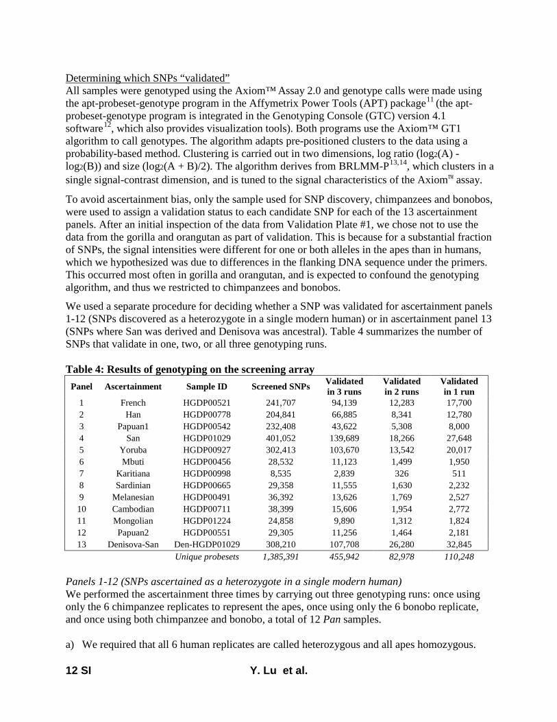
12 SI Y. Lu et al.

Determining which SNPs “validated” All samples were genotyped using the Axiom™ Assay 2.0 and genotype calls were made using the apt-probeset-genotype program in the Affymetrix Power Tools (APT) package11 (the apt-probeset-genotype program is integrated in the Genotyping Console (GTC) version 4.1 software12, which also provides visualization tools). Both programs use the Axiom™ GT1 algorithm to call genotypes. The algorithm adapts pre-positioned clusters to the data using a probability-based method. Clustering is carried out in two dimensions, log ratio (log2(A) - log2(B)) and size (log2(A + B)/2). The algorithm derives from BRLMM-P13,14, which clusters in a single signal-contrast dimension, and is tuned to the signal characteristics of the Axiom™ assay.

To avoid ascertainment bias, only the sample used for SNP discovery, chimpanzees and bonobos, were used to assign a validation status to each candidate SNP for each of the 13 ascertainment panels. After an initial inspection of the data from Validation Plate #1, we chose not to use the data from the gorilla and orangutan as part of validation. This is because for a substantial fraction of SNPs, the signal intensities were different for one or both alleles in the apes than in humans, which we hypothesized was due to differences in the flanking DNA sequence under the primers. This occurred most often in gorilla and orangutan, and is expected to confound the genotyping algorithm, and thus we restricted to chimpanzees and bonobos.

We used a separate procedure for deciding whether a SNP was validated for ascertainment panels 1-12 (SNPs discovered as a heterozygote in a single modern human) or in ascertainment panel 13 (SNPs where San was derived and Denisova was ancestral). Table 4 summarizes the number of SNPs that validate in one, two, or all three genotyping runs. Table 4: Results of genotyping on the screening array

Panel Ascertainment Sample ID Screened SNPs Validated in 3 runs

Validated in 2 runs

Validated in 1 run

1 French HGDP00521 241,707 94,139 12,283 17,700 2 Han HGDP00778 204,841 66,885 8,341 12,780 3 Papuan1 HGDP00542 232,408 43,622 5,308 8,000 4 San HGDP01029 401,052 139,689 18,266 27,648 5 Yoruba HGDP00927 302,413 103,670 13,542 20,017 6 Mbuti HGDP00456 28,532 11,123 1,499 1,950 7 Karitiana HGDP00998 8,535 2,839 326 511 8 Sardinian HGDP00665 29,358 11,555 1,630 2,232 9 Melanesian HGDP00491 36,392 13,626 1,769 2,527 10 Cambodian HGDP00711 38,399 15,606 1,954 2,772 11 Mongolian HGDP01224 24,858 9,890 1,312 1,824 12 Papuan2 HGDP00551 29,305 11,256 1,464 2,181 13 Denisova-San Den-HGDP01029 308,210 107,708 26,280 32,845

Unique probesets 1,385,391 455,942 82,978 110,248 Panels 1-12 (SNPs ascertained as a heterozygote in a single modern human) We performed the ascertainment three times by carrying out three genotyping runs: once using only the 6 chimpanzee replicates to represent the apes, once using only the 6 bonobo replicate, and once using both chimpanzee and bonobo, a total of 12 Pan samples. a) We required that all 6 human replicates are called heterozygous and all apes homozygous.

13 SI Y. Lu et al.

b) We required that the homozygous cluster and heterozygous cluster were well resolved in the clustering space, referred to as “A vs. M space”. M and A are defined as

𝑀 = �𝑙𝑜𝑔2 �𝐴𝑎𝑙𝑙𝑒𝑙𝑒𝑠𝑖𝑔𝑛𝑎𝑙𝑖𝑛𝑡𝑒𝑛𝑠𝑖𝑡𝑦� − 𝑙𝑜𝑔2 �𝐵𝑎𝑙𝑙𝑒𝑙𝑒𝑠𝑖𝑔𝑛𝑎𝑙𝑖𝑛𝑡𝑒𝑛𝑠𝑖𝑡𝑦��

𝐴 = �𝑙𝑜𝑔2 �𝐴𝑎𝑙𝑙𝑒𝑙𝑒𝑠𝑖𝑔𝑛𝑎𝑙𝑖𝑛𝑡𝑒𝑛𝑠𝑖𝑡𝑦� + 𝑙𝑜𝑔2 �𝐵𝑎𝑙𝑙𝑒𝑙𝑒𝑠𝑖𝑔𝑛𝑎𝑙𝑖𝑛𝑡𝑒𝑛𝑠𝑖𝑡𝑦�� /2

Based on the experience of Affymetrix scientists with the Axiom™ 2.0 Assay, five conditions were required to be satisfied to ensure that the clusters were well resolved in clustering space. Using the definitions “hetero”=samples called heterozygous, “homo”=samples called homozygous, “std”=standard error, and “abs”=absolute value, the 5 conditions that we required to be met to consider a SNP as validated were:

(i) 𝑚𝑒𝑎𝑛(𝑀ℎ𝑒𝑡𝑒𝑟𝑜) ∈ (−1,1) and 𝑚𝑒𝑎𝑛(𝑀ℎ𝑜𝑚𝑜) ∈ (−∞,−1] 𝑜𝑟 [1, +∞) (ii) 𝑚𝑒𝑎𝑛(𝐴ℎ𝑒𝑡𝑒𝑟𝑜) − 2 × 𝑠𝑡𝑑(𝐴ℎ𝑒𝑡𝑒𝑟𝑜) > 𝑚𝑒𝑎𝑛(𝐴ℎ𝑜𝑚𝑜) − 2 × 𝑠𝑡𝑑(𝐴ℎ𝑜𝑚𝑜) (iii) 𝑚𝑒𝑎𝑛(𝐴ℎ𝑒𝑡𝑒𝑟𝑜) ≥ 8.5 (iv) Δ sep≥5, where Δsep is computed using the following formula

∆𝑠𝑒𝑝= 𝑎𝑏𝑠 �𝑚𝑒𝑎𝑛(𝑀ℎ𝑜𝑚𝑜) −𝑚𝑒𝑎𝑛(𝑀ℎ𝑒𝑡𝑒𝑟𝑜)[𝑠𝑡𝑑(𝑀ℎ𝑜𝑚𝑜) + 𝑠𝑡𝑑(𝑀ℎ𝑒𝑡𝑒𝑟𝑜)]/2

�

(v) 𝑎𝑏𝑠�𝑚𝑒𝑎𝑛(𝑀ℎ𝑒𝑡𝑒𝑟𝑜)− 𝑚𝑒𝑎𝑛(𝑀ℎ𝑜𝑚𝑜)� > 1

c) We required that the chimpanzee and bonobo agree at least partially in their genotype calls, for SNPs where a call was made in at least one of the three genotyping runs. The goal was to exclude SNPs that completely disagreed between chimpanzees and bonobos, which would imply that the ancestral allele determination was unreliable at these sites.

Panel 13 (SNPs where San was derived and Denisova was ancestral) SNPs were considered as “validated” for panel 13 if they passed the following validation criteria: a) All six San replicates were called heterozygote or derived homozygotes, and all ape replicates

were called ancestral homozygotes. b) SNPs in chromosome X were not in pseudoautosomal regions (PARs) and were called as

homozygous derived in the San individual. (i) PARs were determined by converting coordinates of the human PARs (Build36) to

PanTro2 using the liftOver program from the UCSC genome browser. (ii) The San sample is a male, so SNPs in this chromosome are expected to be homozygotes.

c) The following three criteria were required to be met to make sure that the clusters were located around expected locations and well separated (that is, they were well resolved) (i) 𝑚𝑒𝑎𝑛�𝑀𝑎𝑝𝑒ℎ𝑜𝑚𝑜� ∈ (−∞,−1] 𝑜𝑟 [1, +∞) (ii) 𝑚𝑒𝑎𝑛�𝐴𝑎𝑝𝑒_ℎ𝑜𝑚𝑜� ≥ 9.5 (iii) 𝑠𝑡𝑑�𝑀𝑎𝑝𝑒_ℎ𝑜𝑚𝑜� < 0.45

d) For a SNP passing the above criteria in any one of three genotyping runs, we required that the chimpanzee and bonobo genotypes, compared across runs, did not completely disagree.

For autosomal SNPs in Panel 13, the true genotype for San replicates could be either heterozygote or derived homozygote. To avoid potential bias that might cause either heterozygous or derived

14 SI Y. Lu et al.

homozygous genotypes to be validated at a higher rate, we did not apply any metrics involving measuring the coherence of the heterozygous or derived homozygous clusters. Thus, the criteria used for Panel 13 are looser than the other 12 panels, which we expect will minimize the potential for ascertainment bias at the cost of lowering the validation rate of SNPs. Filtering of SNPs based on the genotyping of 184 samples on Validation Plates #2 and #3 Up to this point, all decisions about which SNPs were considered to be validated were based entirely on the results of genotyping Validation Plate #1 on the screening array. As these decisions were only based on data from apes and the human sample used in SNP discovery, this is a perfectly clean strategy from the point of view of SNP ascertainment. In practice on inspection of the genotyping results for Validation Plates #2 and #3, we found that a small fraction of SNPs that passed the validation filters described above were completely heterozygous in modern humans, or nearly so. This is unexpected based on population genetic considerations, and suggests that these SNPs overlap segmental duplications (which we did not screen out from our array in the interests of having a completely unbiased ascertainment procedure). An observation of more than half of individuals being heterozygous is unexpected at a true SNP. In an unstructured population for a SNP of frequency p, the expected proportion of heterozygous genotypes is 2p(1-p), which is at most 0.5, and the expected rate of heterozygous genotypes is less than this for a structured population. We therefore implemented a further filter where for each SNP, we computed its frequency across all of the N modern humans on Validation Plates #2 and #3 that successfully genotyped (N≥184). We then counted the observed number of heterozygous genotypes hetobs versus the conservative expectation of hetexp = Nphet, where phet = 2p(1-p) (here, p is the empirical frequency of the derived allele, (hetobs+2(number of homozygous genotypes)/2N)). By dividing the difference between the observed and the expected number of heterozygous genotypes by the binomially distributed standard error, we can compute an approximately normally distributed Z-score:

𝑍 =ℎ𝑒𝑡𝑜𝑏𝑠 − ℎ𝑒𝑡𝑒𝑥𝑝�𝑁𝑝ℎ𝑒𝑡(1 − 𝑝ℎ𝑒𝑡)

We filtered out SNPs for which Z > 5, which is expected to remove at most a fraction 3.0×10-7 of true SNPs by chance. This removed 1,932 additional SNPs. Summary of results of the validation genotyping A total of 605,069 unique probesets (599,175 unique SNPs) were validated by the screen. The numbers of validated SNPs in each panel is listed in Table 3. Taking forward SNPs to a final production array All of the 605,069 probesets that passed the validation criteria after genotyping on the screening array were tiled on the final production array. In addition to those 605,069 “Human Origins” SNPs, a set of 87,044 “Compatibility” SNPs were also tiled on the final production array, choosing from a set of 8.8 million SNPs that had previously been validated using the Axiom 2.0TM genotyping assay. Among those SNPs, there are 2,091 non-PAR chromosome Y SNPs, 259 mitochondrial SNPs, and 84,694 SNPs that overlap between the Affymetrix SNP Array 6.0 and Illumina 650Y array. No A/T or C/G SNPs were selected for the Compatibility SNPs, as they take up more space on the array (two probes for each SNP), so that excluding them thus allowed us to

15 SI Y. Lu et al.

maximize information from the array. For the 84,694 nuclear SNPs, we increased the value of the SNPs by maximizing the fraction that were also genotyped on the Affymetrix SNP Array 5.0 (78.5%), that were covered by sequencing from Neandertal (53.9%) and Denisova (64.7%), and for which a chimpanzee allele was available (nearly 100%).

Validation of the final SNP array through genotyping of 952 CEPH-HGDP samples We attempted to genotype 952 CEPH-HGDP samples that were previously determined to be unrelated up to second degree relatives15. This genotyping had three goals:

(a) Round 2 validation: Evaluating the performance of every SNP in the final product array Although all of the SNPs that were tiled on the final product array had previously been validated in screening arrays, there is variability in how an assay performs on a real product. Hence after manufacturing the final SNP array, we genotyped 952 unrelated CEPH-HGDP samples (including the 12 modern human samples used in SNP ascertainment) using the final product array. We used these data to create a list of SNPs that had gone through two rounds of validation and would be robust for genotyping.

(b) Building up prior distributions for SNP calling The Axiom™ GT1 algorithm makes more accurate genotype calling for a SNP if it has prior distributions for the 3 genotype clusters (AA, AB, and BB) based on data (by default, the Axiom™ GT1 algorithm uses the generic prior distributions of the 3 clusters, which is just a best guess). Because the CEPH-HGDP panel has such a large number of samples from diverse ancestries, we expect to observe clusters from all 3 genotypes for most SNPs. This allows us to construct prior distributions that could be used for SNP calling in other projects.

(c) Creating a dataset that will be useful for population genetics The genotyping of the unrelated CEPH-HGDP samples has the benefit that it creates a dataset that will be widely available to the population genetics community. Users who wish to genotype samples that they are interested in on this array, will be able to merge the data that they collect with data collected on the CEPH-HGDP samples, to enable a richer comparison of genetic variation in one region to worldwide variation.

Table 5. Eighteen HGDP samples that did not pass quality control Identifier Population Reason removed HGDP00009 Brahui Failed DQC HGDP00708 Colombian <97% genotype call rate HGDP01266 Mozabite <97% genotype call rate HGDP01267 Mozabite <97% genotype call rate HGDP01403 Adygei <97% genotype call rate HGDP00885 Russian <97% genotype call rate HGDP00886 Russian <97% genotype call rate HGDP00795 Orcadian <97% genotype call rate HGDP00804 Orcadian <97% genotype call rate HGDP00746 Palestinian <99% concordance with Illumina 650Y data HGDP00326 Kalash <99% concordance with Illumina 650Y data HGDP00274 Kalash <99% concordance with Illumina 650Y data HGDP00304 Kalash <99% concordance with Illumina 650Y data HGDP00309 Kalash <99% concordance with Illumina 650Y data HGDP01361 Basque <99% concordance with Illumina 650Y data HGDP00710 Colombian <99% concordance with Illumina 650Y data HGDP01376 Basque <99% concordance with Illumina 650Y data HGDP01009 Karitiana anomalous ancestry relative to others in group

16 SI Y. Lu et al.

Filtering out 18 samples that did not genotype reliably After assaying all 952 samples, we filtered to 934 samples as follows (Table 5): (a) We filtered out 9 samples that did not pass standard Axiom™ 2.0 Array QC metrics: a “DQC”

score (chip-level quality metric) and a call rate score. This suggests problems such as low input DNA amount, contamination of DNA samples, or technical issues with hybridization. These 9 samples were excluded from the genotyping calling.

(b) We excluded an additional 9 samples based on their genotype patterns. Of these, 8 were excluded because there was a greater than 1% genotype discrepancy between our current data and earlier data from the Illumina 650Y array genotyped on the same samplesError! Bookmark not defined.. We also excluded HGDP01009, an individual that our data (as well as analyses of previous datasets) suggests is a sample whose ancestry is an outlier relative to others from the Karitiana group, suggesting a history of recent gene flow with other Native American populations.

Special filters applied to chromosome X and Y data Chromosome X occurs in only a single copy in men but in two copies in women. Chromosome Y occurs only in men. This means that SNPs on these chromosomes need to be treated differently from autosomal SNPs; for chromosome X we genotyped males and females separately, and for chromosome Y we only genotyped males. For males, we required that genotypes on both chromosome X and Y were always homozygous. Filtering out additional probesets based on the genotyping of the final array Not all probesets tiled onto the final array performed well enough to produce reliable results. We filtered out a total of 58,488 additional probesets by sequentially applying the seven criteria listed in Table 6. Three of the criteria used in Table 6 require more detailed explanation. Table 6. Phase 2 validation (determining probesets for which we report genotypes) Order Filter Removed Definition 1 SNP call rate ≥ 95% 23,476 (no. of called samples) / (no. of genotyped samples = 943)

2 Concordance 31,415 For panels 1-12, the SNP must be heterozygous in the sample used in ascertainment (for panel 13, heterozygous or derived homozygous).

3 het_rate > 5 79 This is the same metric used in SNP validation 4 het_offset > -0.5 892 See below for explanation 5 resolution score ≥ 3.6 2,450 See below for explanation 6 chrX annotation 94 Panel 13 SNPs that are PanTro2 chrX but not hg18 chrX are removed.

7 chrX SNPs separate males and females 82 See below for explanation

Total removed by all filters 58,488 het_offset: Using the definition of “A vs. M space” described in the discussion of the screening array filters, we defined a quantity called het_offset that measures whether the heterozygous genotype is appropriately intermediate between the homozygous clusters. For a probeset with three observed genotype clusters (AA, AB, and BB), it is defined as

ℎ𝑒𝑡_𝑜𝑓𝑓𝑠𝑒𝑡: 𝑚𝑒𝑎𝑛(𝑀𝐴𝐵) − 𝑚𝑒𝑎𝑛(𝑀𝐴𝐴)+𝑚𝑒𝑎𝑛(𝑀𝐵𝐵)2

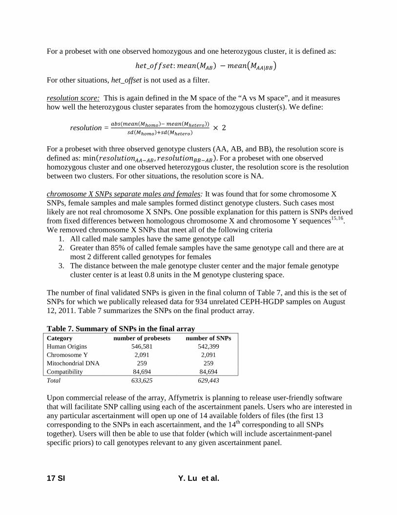
17 SI Y. Lu et al.

For a probeset with one observed homozygous and one heterozygous cluster, it is defined as:

ℎ𝑒𝑡_𝑜𝑓𝑓𝑠𝑒𝑡: 𝑚𝑒𝑎𝑛(𝑀𝐴𝐵) −𝑚𝑒𝑎𝑛�𝑀𝐴𝐴|𝐵𝐵�

For other situations, het_offset is not used as a filter. resolution score: This is again defined in the M space of the “A vs M space”, and it measures how well the heterozygous cluster separates from the homozygous cluster(s). We define: resolution = 𝑎𝑏𝑠(𝑚𝑒𝑎𝑛(𝑀ℎ𝑜𝑚𝑜)− 𝑚𝑒𝑎𝑛(𝑀ℎ𝑒𝑡𝑒𝑟𝑜))

𝑠𝑑(𝑀ℎ𝑜𝑚𝑜)+𝑠𝑑(𝑀ℎ𝑒𝑡𝑒𝑟𝑜) × 2

For a probeset with three observed genotype clusters (AA, AB, and BB), the resolution score is defined as: min(𝑟𝑒𝑠𝑜𝑙𝑢𝑡𝑖𝑜𝑛𝐴𝐴−𝐴𝐵, 𝑟𝑒𝑠𝑜𝑙𝑢𝑡𝑖𝑜𝑛𝐵𝐵−𝐴𝐵). For a probeset with one observed homozygous cluster and one observed heterozygous cluster, the resolution score is the resolution between two clusters. For other situations, the resolution score is NA. chromosome X SNPs separate males and females: It was found that for some chromosome X SNPs, female samples and male samples formed distinct genotype clusters. Such cases most likely are not real chromosome X SNPs. One possible explanation for this pattern is SNPs derived from fixed differences between homologous chromosome X and chromosome Y sequences15,16. We removed chromosome X SNPs that meet all of the following criteria

1. All called male samples have the same genotype call 2. Greater than 85% of called female samples have the same genotype call and there are at

most 2 different called genotypes for females 3. The distance between the male genotype cluster center and the major female genotype

cluster center is at least 0.8 units in the M genotype clustering space.

The number of final validated SNPs is given in the final column of Table 7, and this is the set of SNPs for which we publically released data for 934 unrelated CEPH-HGDP samples on August 12, 2011. Table 7 summarizes the SNPs on the final product array. Table 7. Summary of SNPs in the final array Category number of probesets number of SNPs Human Origins 546,581 542,399 Chromosome Y 2,091 2,091 Mitochondrial DNA 259 259 Compatibility 84,694 84,694 Total 633,625 629,443 Upon commercial release of the array, Affymetrix is planning to release user-friendly software that will facilitate SNP calling using each of the ascertainment panels. Users who are interested in any particular ascertainment will open up one of 14 available folders of files (the first 13 corresponding to the SNPs in each ascertainment, and the 14th corresponding to all SNPs together). Users will then be able to use that folder (which will include ascertainment-panel specific priors) to call genotypes relevant to any given ascertainment panel.

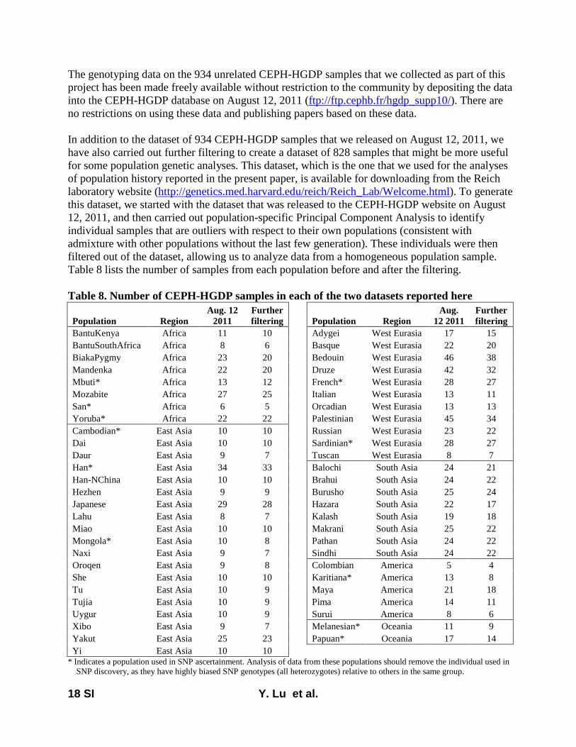
18 SI Y. Lu et al.

The genotyping data on the 934 unrelated CEPH-HGDP samples that we collected as part of this project has been made freely available without restriction to the community by depositing the data into the CEPH-HGDP database on August 12, 2011 (ftp://ftp.cephb.fr/hgdp_supp10/). There are no restrictions on using these data and publishing papers based on these data. In addition to the dataset of 934 CEPH-HGDP samples that we released on August 12, 2011, we have also carried out further filtering to create a dataset of 828 samples that might be more useful for some population genetic analyses. This dataset, which is the one that we used for the analyses of population history reported in the present paper, is available for downloading from the Reich laboratory website (http://genetics.med.harvard.edu/reich/Reich_Lab/Welcome.html). To generate this dataset, we started with the dataset that was released to the CEPH-HGDP website on August 12, 2011, and then carried out population-specific Principal Component Analysis to identify individual samples that are outliers with respect to their own populations (consistent with admixture with other populations without the last few generation). These individuals were then filtered out of the dataset, allowing us to analyze data from a homogeneous population sample. Table 8 lists the number of samples from each population before and after the filtering. Table 8. Number of CEPH-HGDP samples in each of the two datasets reported here

Population Region Aug. 12

2011 Further filtering Population Region

Aug. 12 2011

Further filtering

BantuKenya Africa 11 10 Adygei West Eurasia 17 15 BantuSouthAfrica Africa 8 6 Basque West Eurasia 22 20 BiakaPygmy Africa 23 20 Bedouin West Eurasia 46 38 Mandenka Africa 22 20 Druze West Eurasia 42 32 Mbuti* Africa 13 12 French* West Eurasia 28 27 Mozabite Africa 27 25 Italian West Eurasia 13 11 San* Africa 6 5 Orcadian West Eurasia 13 13 Yoruba* Africa 22 22 Palestinian West Eurasia 45 34 Cambodian* East Asia 10 10 Russian West Eurasia 23 22 Dai East Asia 10 10 Sardinian* West Eurasia 28 27 Daur East Asia 9 7 Tuscan West Eurasia 8 7 Han* East Asia 34 33 Balochi South Asia 24 21 Han-NChina East Asia 10 10 Brahui South Asia 24 22 Hezhen East Asia 9 9 Burusho South Asia 25 24 Japanese East Asia 29 28 Hazara South Asia 22 17 Lahu East Asia 8 7 Kalash South Asia 19 18 Miao East Asia 10 10 Makrani South Asia 25 22 Mongola* East Asia 10 8 Pathan South Asia 24 22 Naxi East Asia 9 7 Sindhi South Asia 24 22 Oroqen East Asia 9 8 Colombian America 5 4 She East Asia 10 10 Karitiana* America 13 8 Tu East Asia 10 9 Maya America 21 18 Tujia East Asia 10 9 Pima America 14 11 Uygur East Asia 10 9 Surui America 8 6 Xibo East Asia 9 7 Melanesian* Oceania 11 9 Yakut East Asia 25 23 Papuan* Oceania 17 14 Yi East Asia 10 10

* Indicates a population used in SNP ascertainment. Analysis of data from these populations should remove the individual used in SNP discovery, as they have highly biased SNP genotypes (all heterozygotes) relative to others in the same group.

19 SI Y. Lu et al.

References

1 Rosenberg NA, Mahajan S, Ramachandran S, Zhao C, Pritchard JK, Feldman MW (2005) Clines, clusters, and the

effect of study design on the inference of human population structure. PLoS Genet. 1,e70. 2 Wang S et al. (2007) Genetic variation and population structure in native American. PLoS Genet. 3, e185. 3 Tishkoff SA et al. (2009) The genetic structure and history of Africans and African Americans. Science. 324, 1035-

44. 4 Friedlaender JS et al. (2008) The genetic structure of Pacific Islanders. PLoS Genet. 4, e19. 5 Rosenberg NA et al. (2006) Low levels of genetic divergence across geographically and linguistically diverse

populations from India. PLoS Genet. 2, e215. 6 Keinan A, Mullikin JC, Patterson N, Reich D (2007) Measurement of the human allele frequency spectrum

demonstrates greater genetic drift in East Asians than Europeans. Nature Genetics 39, 1251-1255 7 Reich D, Green RE, Kircher M, Krause J, Patterson N, Durand EY, Viola B, Briggs AW, Stenzel U, Johnson PLF,

Maricic T, Good JM, Marques-Bonet T, Alkan C, Fu Q, Mallick S, Li H, Meyer M, Eichler EE, Stoneking M, Richards M, Talamo S, Shunkov MV, Derevianko AP, Hublin JJ, Kelso J, Slatkin M & Pääbo S (2010) Genetic history of an archaic hominin group from Denisova Cave in Siberia. Nature 468, 1053-1060.

8 Li JZ et al. (2008) Worldwide human relationships inferred from genome-wide patterns of variation. Science 319, 1100-4. 9 Green RE et al. (2010) A draft sequence of the Neandertal genome. Science 328, 710-722. 10 Cann HM et al. (2002) A human genome diversity cell line panel. Science 296, 261-2. 11 Affymetrix Power Tools: http://www.affymetrix.com/partners_programs/programs/developer/tools/powertools.affx 12 Genotyping Console:

http://www.affymetrix.com/browse/level_seven_software_products_only.jsp?productId=131535&categoryId=35625#1_1

13 Single-sample analysis methodology for the DMET™ Plus Premier Pack - this white paper also applies to the Axiom GT1 genotyping algorithm. http://www.affymetrix.com/support/technical/whitepapers/dmet_plus_algorithm_whitepaperv1.pdf (pdf, 292 KB)

14 BRLMM-P: a Genotype Calling Method for the SNP 5.0 Array http://www.affymetrix.com/support/technical/whitepapers/brlmmp_whitepaper.pdf (pdf, 163 KB)

15 Rosenberg NA (2006) Standardized subsets of the HGDP-CEPH Human Genome Diversity Cell Line Panel, accounting for atypical and duplicated samples and pairs of close relatives. Ann Hum Genet 70, 841-7.

16 Ross MT et al. (2005) The DNA sequence of the human X chromosome. Nature, 434,325-337

2 SI Y. Lu et al.

File S1 Technical details of a SNP array optimized for population genetics

Yontao Lu, Nick Patterson, Yiping Zhan, Swapan Mallick and David Reich

Overview One of the promises of studies of human genetic variation is to learn about human history and also to learn about natural selection. Array genotyping of hundreds of thousands of SNPs simultaneously—using a technology that produces high fidelity data with an error rate of ~0.1%—is in theory a powerful tool for these studies. However, a limitation of all SNP arrays that have been available to date is that the SNPs have been chosen in a complicated way for the purpose of medical genetics, biasing their frequencies so that it is challenging to make reliable population genetic inferences. In general, the way that SNPs have been chosen for arrays is so complicated that it has been effectively impossible to model the ascertainment strategy and thus to correct for the bias. This technical note describes the design, validation, and manufacture of an array consisting of SNPs all ascertained in a clearly documented way. We anticipate that this will provide a useful resource for the community interested in learning about history and natural selection. We hope that this array will be genotyped in many different cohorts, as has been done, for example, in the Marshfield panel where approximately 800 microsatellites have been genotyped in diverse populations1,2,3,4,5. By establishing a common set of simply ascertained SNPs that have been genotyped in diverse populations, it should be possible to learn about human history not only in individual studies, but also through meta-analysis. The array is designed as a union of 13 different SNP panels. In our experience, a few tens of thousands of SNPs is enough to produce powerful inferences about history with regard to summary statistics like measurements of FST. Thus, it is better for many analyses to have (for example) 13 sets of tens to hundreds of thousands of SNPs each with its own ascertainment strategy than a single set of 600,000 SNPs. We have included a particularly large number of SNPs from particularly interesting ascertainments—discovery in the two chromosomes of a single San Bushman, a single Yoruba West African, a single French, a single Han Chinese, and a single Papuan—as for some analyses like scans of selection it is valuable to have dense data sets of hundreds of thousands of SNPs. All SNPs chosen for the array were selected from sites in the genome that have read coverage from Neandertals, Denisovans, and chimpanzees, allowing users of the array to compare data from modern humans to archaic hominins and apes. This array is not ideal for gene mapping, since: (i) No attempt has been made to tag common variation genome-wide. (ii) There are gaps in the genome where no homologous sequence is available from chimpanzee. (iii) Unlike many existing arrays, we have not oversampled SNPs in the vicinity of genes, or adjusting SNP density in order to fully tag haplotypes. Instead we simply sampled SNPs in proportion to their genomic density as discovered by sequencing. The array is being made commercially available by Affymetrix. Importantly, the academic collaborators who have been involved in the design will not benefit from sales of the array (they

3 SI Y. Lu et al.

will not receive any financial compensation from Affymetrix). The CEPH-Human Genome Diversity Project (CEPH-HGDP) samples that were genotyped during the course of the project will not be used for any commercial purposes. Affymetrix deposited the genotypes of unrelated CEPH-HGDP samples, collected as part of the array development, into the CEPH-HGDP database on August 12, 2011, more than six months before commercial release of the array (in Spring 2012), and this genotyping data is freely available to the public. Design strategy for the 13 panels (Panels 1-12) Discovery of heterozygous sites within 12 individuals of known ancestry The first 12 SNP ascertainment strategies are based on the idea of the Keinan, Mullikin et al. Nature Genetics 2007 paper6. That paper takes advantage of the fact that by discovering SNPs in a comparison of two chromosomes from the same individual of known ancestry, and then genotyping in a larger panel of samples from the same population, one can learn about history in a way that is not affected by the frequency of the SNP in human populations. In particular, even though we may miss a substantial proportion of real SNPs in the individual (false-negatives), and even if a substantial proportion of discovered SNP are false-positives, we expect that the inferences about history using SNPs discovered in this way will be as accurate as what would be obtained using SNPs identified from deep sequencing with perfect readout of alleles. To understand why false-negative SNPs should not bias inferences, we note that if a SNP is truly heterozygous in the individual in whom we are trying to discover it, there is exactly one copy of the ancestral allele and exactly one copy of the derived allele. Thus, conditional on the SNP being heterozygous in the discovery individual, its probability of being discovered is not further affected by whether it has a high or low minor allele frequency in the population. This contrasts with ascertainment strategies that discover SNPs in more than one individual, where there is always a real (and extremely difficult to quantify) bias toward missing rarer variants. By genotyping SNPs discovered in this way, and making a simple p(1-p) correction for discovery in two chromosomes (where p is the minor allele frequency), one can obtain an unbiased reconstruction of the allele frequency distribution in the population. An important feature of this SNP discovery strategy is that false-positive SNPs (for example, due to sequencing error, mapping error, segmental duplications or copy number variation) are not expected to substantially bias inferences. The reason is that we have validated all candidate SNPs by genotyping them using a different technology, and we have required the genotypes to match the individuals in whom they were discovered. Thus, we expect to have a negligible proportion of false-positive SNPs on the final array. This procedure has produced 12 panels of uniformly discovered SNPs, which can be used for allele frequency spectrum analysis. There is some overlap of SNPs across panels. Importantly, we have separately determined validation status for the SNPs in each panel, and have only used SNPs that validate in the same sample in which they were discovered. Thus, we have not biased toward SNPs with a high minor allele frequency, or that are polymorphic across multiple populations, which might be expected to have a higher chance of validation if we did not perform the validation in each discovery sample independently.

4 SI Y. Lu et al.

(Panel 13) SNPs where a randomly chosen San allele is derived relative to an archaic hominin A 13th ascertainment strategy used alignments of three genomes: chimpanzee, Denisova (an archaic hominin from southern Siberia for whom there is 1.9× genome sequence coverage7), and San. We examined sites where we had ≥1-fold coverage of Denisova, and ≥3-fold coverage of San. We made an allele call for each individual by majority rule, randomly selecting an allele when there was a tie (this means that we are effectively sampling one of two haplotypes in the individual, and the allele call is not expected to be being biased if the individual is heterozygous at that site). We placed on the array the subset of sites where San is derived relative to both Denisova and chimpanzee, in this case requiring agreement between the Denisova and chimpanzee allele. These are sites that likely arose due to mutations in the last million years. We chose to use San rather than another modern human for building this panel because there is evidence that the San are approximately symmetrically related to all other present-day humans8. Panel 13 is also the only one with SNPs from chromosome X (all the other panels are based on SNPs discovered in males), and thus this panel permits X-autosome comparisons. Description of the sequencing data and filtering used in SNP ascertainment The sequencing data that we use for identifying candidate SNPs has been described in two recent papers: Green et al. 20109 and Reich et al. 20107. The data were all generated in the Max Planck Institute in Leipzig using Illumina Genome Analyzer IIx (GAIIx) sequencing instruments via protocols that are described in refs. 9 and 7 (Table 1). Population genetic analyses for ref. 7 were carried out on the very data file that was used to select SNPs for the array. Table 1: Characteristics of the sequencing data we are using for SNP ascertainment

Name Identifier Sequenced by Genomic coverage*

Cutoff† A (Pr)

Cutoff† C (Pr)

Cutoff† G (Pr)

Cutoff† T (Pr)

Han HGDP00778 Green 2010 3.8 16 (0.489) 14 (0.239) 17 (0.003) 15 (0.11)

Papuan1 HGDP00542 Green 2010 3.6 13 (0.051) 10 (0.119) 15 (0.434) 13 (0.880)

Yoruba HGDP00927 Green 2010 4.3 17 (0.692) 14 (0.440) 18 (0.562) 16 (0.985)

San HGDP01029 Green 2010 5.9 17 (0.830) 15 (0.914) 18 (0.649) 16 (0.877)

French HGDP00521 Green 2010 4.4 17 (0.317) 16 (0.985) 18 (0.024) 17 (0.515)

Mbuti HGDP00456 Reich 2010 1.2 17 (0.041) 14 (0.504) 17 (0.704) 16 (0.379)

Karitiana HGDP00998 Reich 2010 1.1 18 (0.210) 14 (0.126) 17 (0.147) 17 (0.589)

Sardinian HGDP00665 Reich 2010 1.3 19 (0.789) 15 (0.302) 18 (0.474) 17 (0.200)

Bougainville HGDP00491 Reich 2010 1.5 18 (0.810) 14 (0.288) 17 (0.445) 16 (0.291)

Cambodian HGDP00711 Reich 2010 1.7 18 (0.717) 14 (0.303) 17 (0.331) 16 (0.398)

Mongolian HGDP01224 Reich 2010 1.4 18 (0.371) 15 (0.789) 17 (0.051) 16 (0.090)

Papuan2 HGDP00551 Reich 2010 1.4 17 (0.188) 14 (0.661) 17 (0.932) 16 (0.885)

Neandertal Vindija.3.bones Green 2010 1.3 27 (0.428) 26 (0.049) 27 (0.308) 27 (0.579)

Denisova Phalanx Reich 2010 1.9 40 (1.000) 40 (1.000) 40 (1.000) 40 (1.000)

* Genomic coverage is calculated for the modern humans as (# of reads mapping to chimpanzee) × (read length which is 76bp for Green et al. 2010 and 101bp for Reich et al. 2010) × (0.95 as we filtered out the 5% of the lowest quality data) / (2.8 Gb). For the archaic hominins we report the coverage from the abstracts of Green et al. 2010 and Reich et al. 2010.

† For each base used in SNP discovery, we give the quality score cutoff and probability of acceptance at that cutoff (parentheses). The cutoffs are chosen to filter out the data of the lowest 5% quality for each nucleotide class (SI 6; Reich et al. 2010).

5 SI Y. Lu et al.

The 12 modern human samples are all from the CEPH-HGDP panel. A valuable feature of this panel is that DNA for all samples is available on request on a cost-recovery basis for researchers who wish to carry out further sequencing and genotyping analysis on these samples for the purpose of research into human population history8,10. Five of the samples (San, Yoruba, Han, French and a Papuan) were sequenced by Green et al. 2010 using Illumina paired-end 76bp reads9, while the remaining 7 (Mbuti, Sardinian, Karitiana, Mongolian, Cambodian, Bougainville, and a second Papuan) were sequenced by Reich et al. 2010 using Illumina paired-end 101bp reads7. All reads from all 12 samples were mapped to chimpanzee (PanTro2). To filter the sequence data for analysis, we used a similar procedure as described in Reich et al. 20107, removing the lowest quality of 5% of nucleotides on a sample and nucleotide-specific basis to maximize the amount of sequencing data available for analysis. After this procedure, we had 3.6-5.9× coverage for the 5 samples and 1.1-1.7× for the 7 samples (Table 1). We also used data from 4 ancient DNA samples to aid our choice of SNPs. To represent Neandertals, we used a pool of sequences from 3 bones from Vindija Cave in Croatia (Vi33.16, Vi33.25 and Vi33.26) for which we had 1.3× genome coverage altogether9. To represent Denisovans, we used data from a finger bone (fifth distal manual phalanx) from the Altai mountains of southern Siberia, with 1.9× coverage7. All reads are mapped to chimpanzee and a chimpanzee allele is available We mapped sequencing reads from modern and ancient genomes to the chimpanzee reference sequence (PanTro2) to avoid biases toward one present-day human group more than another. We filtered out reads with a substantial probability of poor mapping Each read that we analyzed had a mapping quality score (MAPQ) that reflects the confidence of its mapping to PanTro2. Based on empirical exploration of the usefulness of the scores, which were generated by either the ANFO or BWA software, we only used reads that had MAPQ of at least 90 for Neandertal (ANFO mapping), 37 for Denisova (BWA), and 60 for present-day humans (BWA). We also rejected reads if the alignment to the chimpanzee resulted in any insertion/deletion difference. This filter was applied in addition to the filtering of Table 1. Filtering of sites with ≥2 alleles not matching chimp across the humans used for SNP discovery. At a small proportion of sites, we observe more than one non-ancestral allele in the individual sequencing data used for SNP discovery. Such sites cannot be due to a single historical mutation. Instead, the data must reflect at least two mutations or sequencing errors. We filter out such sites. For a very small fraction of sites, we found that the derived allele is different depending on which human is used in SNP discovery (these are potentially triallelic SNPs in the population, although they are not triallelic in the discovery individual). We keep such sites in our list of SNPs for designing, and use multiple probe sets to assay such SNPs.

The raw data file that emerges from this process is available on the “orchestra” Harvard Medical School filesystem at: /groups/reich/CLEAN_SNP_ARRAY/rawsnps and is freely available from David Reich on request (a README file is in the same directory at rawsnps_readme) (Table 2). For brevity, this file only lists the 2,173,116 SNPs where 2 copies of the derived and 1 copy of the ancestral allele are observed a hominin; these are the only SNPs that are candidates for inclusion. Thus, it is an abbreviated version of a larger file used in analyses for ref. 7.

6 SI Y. Lu et al.

Filtering the nucleotide calls of the lowest reliability (a) We do not use nucleotides for which there is no valid nucleotide call for chimpanzee. (b) For Neandertals, we do not use nucleotides within 5 nucleotides of either end of the reads,

because of the elevated rate of ancient DNA degradation errors that we empirically observe. (c) For Denisova, we do not use nucleotides within 1 nucleotide of either end of the read. (d) For both Neandertals and Denisova, we do not use nucleotides with sequence quality <40. (e) For present-day humans, we do not use nucleotides with sequence quality <Tij, where Tij is a

threshold chosen such that half of nucleotides generated from individual i and of allele class j {j = A, C, G, T} are less than this value. For nucleotides that have exactly a quality score of Tij, we randomly choose ones to eliminate such that exactly 5% are dropped (note that this differs from the 50% used in Reich et al. 2010). The cutoffs used are presented in Table 1.

(f) For the “Papuan1” individual from ref. 9 (HGDP00542), the sequencer had a high error rate at position 34 (41 on the reverse strand). We excluded data from position 34 for this individual.

Table 2: Datafiles summarizing the SNP ascertainment for the population genetics array

File name Readme Description Entries

rawsnps rawsnps_readme

This file contains all sites where there are at least 2 copies of a derived allele and 1 copy of the ancestral allele in 12 present-day humans, 3 Neandertals, and Denisova, and further filtered

to be candidates for inclusion in the SNP array.

2, 173,116

ascertained ascertained_readme This file contains all SNPs chosen in any ascertainment panel (there are a few hundred that are triallelic and we list them on different lines, so the number of unique SNPs is 1,812,990).

1,813,579

screening screening_readme

This file contains all probesets we considered for screening array design, as well as the metrics for prioritization and

indicator variables indicating whether they were chosen. If chosen, a column indicates the genotyping outcome, and

whether the SNP was taken forward to the production array.

3,882,158

Note: These files can be found in the Harvard Medical School orchestra filesystem at /groups/reich/CLEAN_SNP_ARRAY/. 1,353,671 SNPs for testing on an Affymetrix Axiom™ screening array 1,812,990 candidate SNPs discovered in 13 different ascertainment panels We used the following algorithm to choose candidate SNPs for validating on the array. (a) We mapped all reads used for SNP discovery to the chimpanzee reference sequence, PanTro2,

without using data from the human reference sequence at all for read mapping. This was important to avoid biases due to the ancestry of the human reference sequence.

(b) We rediscovered all SNPs de novo, blinding ourselves to any prior information about whether

the sites were polymorphic in present-day humans.

(c) At all SNPs, we required coverage from at least 1 Neandertal read and at least 1 Denisova read. This is expected to result in bias toward locations of the genome where the ancient DNA tends to be better preserved or the sequencing technology tends to work better. However, there is no reason why it would be expected to result in a bias in allele frequencies toward one

7 SI Y. Lu et al.

modern human population more than another (as all Neandertal and Denisova reads are mapped to chimpanzee, and no modern human data influences the mapping). The availability of data from archaic hominins from each of the SNPs on our array should be of value for some types of population genetic analysis. (For a handful of sites, the Denisova and Neandertal alleles may not be the same as those seen in present-day humans, but we nevertheless considered these sites to be covered by Denisova and Neandertal as we were concerned that not doing so could introduce bias. Users can treat such sites how they wish.)

(d) All A/T and C/G polymorphisms were excluded, since genotyping these SNPs requires twice

the number of probes using the Axiom™ technology. Thus, removing them increases the number of SNPs we can include on a single array. Removing these SNPs has the additional benefit that it eliminates any strand ambiguity. (Illumina arrays do not genotype A/T or C/G SNPs, either.) However, it also had the disadvantage that A/T and C/G SNPS constitute the one class of SNPs that is believed to be immune to biased gene conversion. Thus, in population genetic analyses of the data generated from the array, it will be important to assess whether inferences are potentially explained by biased gene conversion.

(e) For the SNPs for panels 1-12 (candidate heterozygotes in an individual of known ancestry),

we required the observation of at least 2 copies of the derived (non-chimpanzee) and at least 1 copy of the ancestral allele in the studied person (Reich et al. 2010; SI 6). We did not include chromosome X SNPs from these panels as the 12 individuals were all male.

(f) For the SNPs in panel 13 (derived in San relative to Denisova), we restricted to sites where we

had ≥3-fold read coverage of San and ≥1-fold read coverage of Denisova. A complication in choosing SNPs discovered in two individuals is that both the San and

Denisova individuals are diploid. What we want is to have a panel of SNPs ascertained by comparing a single haploid Denisovan and a single haploid San chromosome, but if we are not careful, we are going to be biased toward the SNPs that are fixed differences. For example, if we accepted only SNPs where all Denisova reads matched chimpanzee and all San reads were derived, then we would bias against SNPs that were truly heterozygous.

To obtain data of the type that would be expected from sampling a single haploid Denisovan and a single haploid San chromosome, we picked the allele that was seen more often in each sample to represent that sample (if there was a tie in terms of the number of reads supporting each allele, we chose one allele at random). In this way, we are picking one of the two chromosomes from each individual (at random), and hence we are effectively sampling a haploid chromosome despite having diploid data. An additional benefit of using the majority rule is that we are also increasing the quality and reliability of the allele call, such that we expect a larger proportion of these SNPs to be real than in panels 1-12.

From the SNPs discovered in this way, we restrict our analysis to sites where Denisova matches the chimpanzee allele and where San is derived (we throw away sites where San is ancestral and Denisova is derived). The reason for this is that this is the only subset of SNPs that we can experimentally validate. To validate these SNPs, we can genotype the San individual and require the observation of an allele that differs from chimpanzee. In contrast, we cannot validate sites where San is ancestral and Denisova is derived, since the Denisova sample is extremely limited and does not provide enough for genotyping assays.

Some of the SNPs from panels 1-13 overlap. Thus, while the sum of the number of SNPs in each panel is 2,581,282, the number of unique SNPs is only 1,812,990. However, the fact that a SNP is

8 SI Y. Lu et al.

present in more than one panel does not mean that it has a higher likelihood of being validated for the array for a given ascertainment strategy. For SNP identified in more than one panel, we designed a single probe to test the SNP, but we assessed its validation status separately for each panel to avoid bias toward more easily validating more polymorphic SNPs (see below). The perl script used for choosing SNPs is on the “orchestra” Harvard Medical School filesystem at: /groups/reich/CLEAN_SNP_ARRAY/newformat_affypick.pl (available on request from David Reich). The output file is at /groups/reich/CLEAN_SNP_ARRAY/ascertained (available on request from David Reich). This list contains a single entry for each unique SNP, with the exception of triallelic sites that have multiple designs (thus, there are 1,813,579 entries rather than 1,812,990). A readme file is at /groups/reich/CLEAN_SNP_ARRAY/ascertained_readme (available on request from David Reich) (Table 2). The number of SNPs that we selected using each strategy is summarized in Table 3. Table 3: Ascertainment of SNPs for panels 1-13

Panel no.

Ascertain-ment Sample ID Genomic

coverage # SNPs found

# SNPs placed on screening

array

# SNPs that validate on screening

array

# SNPs that

validate on final array

1 French HGDP00521 4.4 333,492 241,707 123,574 111,970 2 Han HGDP00778 3.8 281,819 204,841 87,515 78,253 3 Papuan1 HGDP00542 3.6 312,941 232,408 56,518 48,531 4 San HGDP01029 5.9 548,189 401,052 185,066 163,313 5 Yoruba HGDP00927 4.3 412,685 302,413 136,759 124,115 6 Mbuti HGDP00456 1.2 39,178 28,532 14,435 12,162 7 Karitiana HGDP00998 1.1 12,449 8,535 3,619 2,635 8 Sardinian HGDP00665 1.3 40,826 29,358 15,260 12,922 9 Melanesian HGDP00491 1.5 51,237 36,392 17,723 14,988 10 Cambodian HGDP00711 1.7 53,542 38,399 20,129 16,987 11 Mongolian HGDP01224 1.4 35,087 24,858 12,872 10,757 12 Papuan2 HGDP00551 1.4 40,996 29,305 14,739 12,117 13 Denisova-San Den-HGDP01029 - 418,841 308,210 166,422 151,435

Unique SNPs 1,812,990 1,354,003 599,175 542,399

Unique probe designs 1,941,079 1,385,672 605,069 546,581 1,941,079 unique flanking sequences corresponding to the 1,812,990 unique SNPs To ensure clean SNP ascertainment, we followed a rigorous procedure whereby the flanking sequence assay for each SNP were chosen only based on sequencing data from chimpanzee and the modern human sample used in SNP ascertainment. Thus, while some SNPs were discovered in multiple panels, we did not use this information in probe design. We used the simple rules below to pick a probe, and if the optimal design was different depending on the sample in which the SNP was ascertained, we used more than one probe for the SNP. For each SNP in each of the 13 ascertainment panels, we specified 71 base pair (bp) flanking sequences that would be used for probe designing as follows: (a) Ancestral and derived allele are specified based on the individuals used in SNP ascertainment.

For each SNP in each panel, we specified the ancestral and derived alleles based on the two

9 SI Y. Lu et al.

alleles observed in SNP ascertainment, defining as “ancestral” the allele that matched chimpanzee. SNPs within any ascertainment panel almost always had two observed alleles, since we filtered out sites with three or more. However, for SNPs that were discovered in multiple panels, we performed the specification of the ancestral and derived allele independently, and thus for a small fraction of sites, there was a different derived allele depending on the ascertainment panel (even if flanking sequence were sometimes identical).

(b) Flanking sequence is specified entirely based on the modern sample used for SNP discovery.

For initial probe design, we provided 35 bp of flanking sequence on either side of the SNP. We started with 71 bp of sequence from the chimpanzee genome, PanTro2, centered on the SNP. To decrease the number of mismatches between the flanking sequence and any human that might be analyzed using the array, we “humanized” the flanking sequence based on the modern sample used for SNP discovery (importantly, only the discovery sample is used for the humanization of the sequence, and so the ancestry of other samples cannot bias results).

Specifically, for each of panels 1-13, we took all reads from the modern human used in SNP ascertainment that mapped to the flanking nucleotide. Where 100% of reads disagreed with PanTro2, we edited the flanking sequence to reflect that in the ascertainment sample. Otherwise, we kept the chimpanzee allele. An example is: “acctggctccagGgccagcagctccgtcaAggtcc[G/A]ctgcatgaaactgatgaaggggagggcaccaggcg”. Here, capital [G/A] indicates the [chimp/alternate allele] at the SNP and other capital letters indicate bases edited from the chimpanzee reference to match the ascertainment sample. For ascertainment panel 13 (Denisova ancestral and a randomly chosen San allele derived), we did not use the Denisova genome in primer editing. Instead, we edited the sequence to match San whenever San consistently had a non-chimpanzee allele at all reads overlapping the site.

Because the steps above sometimes result in different flanking sequences for the same nucleotide (depending on the particular sequencing reads from the sample used in SNP ascertainment), we were left with more unique flanking sequences (n=1,941,079) than unique SNPs (n=1,812,991).

Procedure used to choose 1,385,671 oligonucleotide probes for the screening array With the list of 1,951,079 flanking sequences, we needed to design oligonucleotide probes, or “probesets”, for a screening array. We blinded ourselves to prior knowledge about which probes worked in previous assays using the Axiom™ technology, since doing so would expected to lead to a higher validation success rate for probes that have been previously tried on SNP arrays (introducing complex biases). For the same reason, we did not modify probe design based on using information in databases about polymorphism in flanking sequence. The only two types of information that were used in probe design were the physical chemistry considerations of which probes are expected to work well, and mapping information to the PanTro2 chimp genome. All the metrics used are in a file on the “orchestra” Harvard Medical School filesystem /groups/reich/CLEAN_SNP_ARRAY/probesets, available on request from David Reich (Table 2). Details of the filtering procedure that we applied are as follows:

(a) We first identified 3,882,158 candidate probesets (two 30mers for each flanking sequence)

For each of the 1,941,079 flanking sequences, it is possible to design two probesets corresponding to the 30 bp 5’ or 3’ direction of the SNP. We use the shorthand “red” to designate the 5’ probe and “green” to designate the 3’ probe, always referenced relative to the positive strand of the chimpanzee genome sequence PanTro2 (Figure 1).

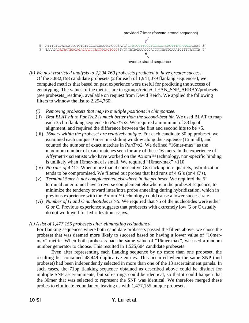
10 SI Y. Lu et al.

(b) We next restricted analysis to 2,294,760 probesets predicted to have greater success Of the 3,882,158 candidate probesets (2 for each of 1,941,079 flanking sequences), we computed metrics that based on past experience were useful for predicting the success of genotyping. The values of the metrics are in /groups/reich/CLEAN_SNP_ARRAY/probesets (see probesets_readme), available on request from David Reich. We applied the following filters to winnow the list to 2,294,760:

(i) Removing probesets that map to multiple positions in chimpanzee. (ii) Best BLAT hit to PanTro2 is much better than the second-best hit. We used BLAT to map

each 35 bp flanking sequence to PanTro2. We required a minimum of 33 bp of alignment, and required the difference between the first and second hits to be >5.

(iii) 16mers within the probeset are relatively unique. For each candidate 30 bp probeset, we examined each unique 16mer in a sliding window along the sequence (15 in all), and counted the number of exact matches in PanTro2. We defined “16mer-max” as the maximum number of exact matches seen for any of these 16-mers. In the experience of Affymetrix scientists who have worked on the Axiom™ technology, non-specific binding is unlikely when 16mer-max is small. We required “16mer-max” <110.

(iv) No runs of 4 G’s. When more than 4 consecutive Gs stack up into quartets, hybridization tends to be compromised. We filtered out probes that had runs of 4 G’s (or 4 C’s),

(v) Terminal 5mer is not complemented elsewhere in the probeset. We required the 5’ terminal 5mer to not have a reverse complement elsewhere in the probeset sequence, to minimize the tendency toward inter/intra probe annealing during hybridization, which in previous experience with the Axiom™ technology could cause a lower success rate.

(vi) Number of G and C nucleotides is >5. We required that >5 of the nucleotides were either G or C. Previous experience suggests that probesets with extremely low G or C usually do not work well for hybridization assays.

(c) A list of 1,477,155 probesets after eliminating redundancy For flanking sequences where both candidate probesets passed the filters above, we chose the probeset that was deemed more likely to succeed based on having a lower value of “16mer-max” metric. When both probesets had the same value of “16mer-max”, we used a random number generator to choose. This resulted in 1,525,604 candidate probesets.

Even after representing each flanking sequence by no more than one probeset, the resulting list contained 48,449 duplicative entries. This occurred when the same SNP (and probeset) had been independently selected in more than one of the 13 ascertainment panels. In such cases, the 71bp flanking sequence obtained as described above could be distinct for multiple SNP ascertainments, but sub-strings could be identical, so that it could happen that the 30mer that was selected to represent the SNP was identical. We therefore merged these probes to eliminate redundancy, leaving us with 1,477,155 unique probesets.

11 SI Y. Lu et al.

Our naming scheme for probesets contains a binary string of 13 characters providing the ascertainment information for that probe. Because we merged some probesets, we created a new ascertainment code called “asc.new”. This was generated by applying a bitwise-or operation to the binary strings of 13 characters corresponding to the ascertainment information for the redundant probes.

(d) A final list of 1,385,672 probes that were placed on the screening array

The 1,477,155 probes that passed our filters were more than could fit into the screening array. Thus, we ranked all the probes based on their “16mer-max” score, breaking ties using a random number generator (lower values have a higher rank). After this ranking, all probes had “16mer-max” of no more than 110, and we were left with 1,385,672 probes.

Design, genotyping, and analysis of screening array Design of the screening array We designed two arrays to screen these 1.39 million probesets (0.69 million probesets fit onto a single screening array). To minimize bias, we randomized the probes with respect to which one of the 2 screening arrays was used to test them. We also used standard chip design strategies that are applied at Affymetrix for determining probe location in each screen design. The number of SNPs from each panel placed on the screening arrays is presented in Table 3. The probesets used in the screening array are named like [chr]_[pos]_[alleles]_[asc.new]_[strand], with the 5 data fields indicating PanTro2 chromosome / PanTro2 physical position / ancestral-derived alleles, and the 13 bit binary string indicating the ascertainment panels in which the SNP was discovered, and the strand (f=forward or r=reverse compared to PanTro2). Genotyping the screening array Three 96-well plates of samples were genotyped on the 2 screening arrays in early 2011, with the goals of (a) deciding if each SNP passes quality control criteria and can be taken forward to the production array, and (b) generating useful data for preliminary population genetic analysis. Validation plate #1: The goal of validation plate #1 was to genotype the same 12 modern human samples that were used in SNP discovery and in which the derived allele was observed, and to validate that we observe an allele at these samples that is distinct from the ancestral allele seen in primates. There was a high level of redundancy on the plate:

• Each of the 12 modern human samples was genotyped 6 times (six different wells) • The chimpanzee and bonobo were each genotyped 6 times • The gorilla and orangutan were each genotyped 4 times

The position of each sample on the plate (except for the upper right 4 wells which were left empty for control samples) was assigned using a random number generator.

Validation plates #2 and #3: We also took advantage of the screening array to genotype 2 plates of samples from CEPH-HGDP populations. We genotyped 184 samples from the same populations that were used in SNP discovery, consisting of French (n=28), Han (n=27), Papuan (n=17), San (n=6), Yoruba (n=21), Mbuti (n=13), Karitiana (n=13), Sardinian (n=28), Melanesian (n=11), Cambodian (n=10) and Mongola (n=10). Analysis of the data allowed us to perform further validation of the SNPs on the array, and also to assess whether useful population genetic analyses can be generated from these genotyping data.

12 SI Y. Lu et al.

Determining which SNPs “validated” All samples were genotyped using the Axiom™ Assay 2.0 and genotype calls were made using the apt-probeset-genotype program in the Affymetrix Power Tools (APT) package11 (the apt-probeset-genotype program is integrated in the Genotyping Console (GTC) version 4.1 software12, which also provides visualization tools). Both programs use the Axiom™ GT1 algorithm to call genotypes. The algorithm adapts pre-positioned clusters to the data using a probability-based method. Clustering is carried out in two dimensions, log ratio (log2(A) - log2(B)) and size (log2(A + B)/2). The algorithm derives from BRLMM-P13,14, which clusters in a single signal-contrast dimension, and is tuned to the signal characteristics of the Axiom™ assay.

To avoid ascertainment bias, only the sample used for SNP discovery, chimpanzees and bonobos, were used to assign a validation status to each candidate SNP for each of the 13 ascertainment panels. After an initial inspection of the data from Validation Plate #1, we chose not to use the data from the gorilla and orangutan as part of validation. This is because for a substantial fraction of SNPs, the signal intensities were different for one or both alleles in the apes than in humans, which we hypothesized was due to differences in the flanking DNA sequence under the primers. This occurred most often in gorilla and orangutan, and is expected to confound the genotyping algorithm, and thus we restricted to chimpanzees and bonobos.

We used a separate procedure for deciding whether a SNP was validated for ascertainment panels 1-12 (SNPs discovered as a heterozygote in a single modern human) or in ascertainment panel 13 (SNPs where San was derived and Denisova was ancestral). Table 4 summarizes the number of SNPs that validate in one, two, or all three genotyping runs. Table 4: Results of genotyping on the screening array

Panel Ascertainment Sample ID Screened SNPs Validated in 3 runs

Validated in 2 runs

Validated in 1 run

1 French HGDP00521 241,707 94,139 12,283 17,700 2 Han HGDP00778 204,841 66,885 8,341 12,780 3 Papuan1 HGDP00542 232,408 43,622 5,308 8,000 4 San HGDP01029 401,052 139,689 18,266 27,648 5 Yoruba HGDP00927 302,413 103,670 13,542 20,017 6 Mbuti HGDP00456 28,532 11,123 1,499 1,950 7 Karitiana HGDP00998 8,535 2,839 326 511 8 Sardinian HGDP00665 29,358 11,555 1,630 2,232 9 Melanesian HGDP00491 36,392 13,626 1,769 2,527 10 Cambodian HGDP00711 38,399 15,606 1,954 2,772 11 Mongolian HGDP01224 24,858 9,890 1,312 1,824 12 Papuan2 HGDP00551 29,305 11,256 1,464 2,181 13 Denisova-San Den-HGDP01029 308,210 107,708 26,280 32,845

Unique probesets 1,385,391 455,942 82,978 110,248 Panels 1-12 (SNPs ascertained as a heterozygote in a single modern human) We performed the ascertainment three times by carrying out three genotyping runs: once using only the 6 chimpanzee replicates to represent the apes, once using only the 6 bonobo replicate, and once using both chimpanzee and bonobo, a total of 12 Pan samples. a) We required that all 6 human replicates are called heterozygous and all apes homozygous.

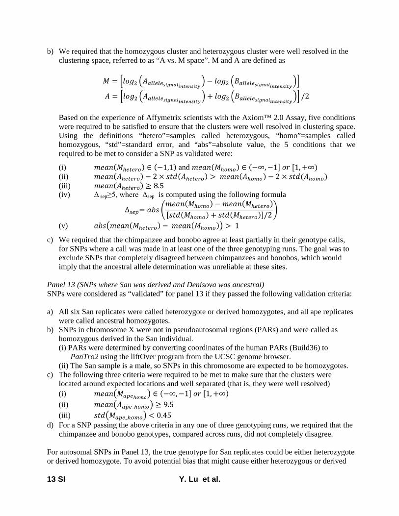
13 SI Y. Lu et al.

b) We required that the homozygous cluster and heterozygous cluster were well resolved in the clustering space, referred to as “A vs. M space”. M and A are defined as

𝑀 = �𝑙𝑜𝑔2 �𝐴𝑎𝑙𝑙𝑒𝑙𝑒𝑠𝑖𝑔𝑛𝑎𝑙𝑖𝑛𝑡𝑒𝑛𝑠𝑖𝑡𝑦� − 𝑙𝑜𝑔2 �𝐵𝑎𝑙𝑙𝑒𝑙𝑒𝑠𝑖𝑔𝑛𝑎𝑙𝑖𝑛𝑡𝑒𝑛𝑠𝑖𝑡𝑦��

𝐴 = �𝑙𝑜𝑔2 �𝐴𝑎𝑙𝑙𝑒𝑙𝑒𝑠𝑖𝑔𝑛𝑎𝑙𝑖𝑛𝑡𝑒𝑛𝑠𝑖𝑡𝑦� + 𝑙𝑜𝑔2 �𝐵𝑎𝑙𝑙𝑒𝑙𝑒𝑠𝑖𝑔𝑛𝑎𝑙𝑖𝑛𝑡𝑒𝑛𝑠𝑖𝑡𝑦�� /2

Based on the experience of Affymetrix scientists with the Axiom™ 2.0 Assay, five conditions were required to be satisfied to ensure that the clusters were well resolved in clustering space. Using the definitions “hetero”=samples called heterozygous, “homo”=samples called homozygous, “std”=standard error, and “abs”=absolute value, the 5 conditions that we required to be met to consider a SNP as validated were:

(i) 𝑚𝑒𝑎𝑛(𝑀ℎ𝑒𝑡𝑒𝑟𝑜) ∈ (−1,1) and 𝑚𝑒𝑎𝑛(𝑀ℎ𝑜𝑚𝑜) ∈ (−∞,−1] 𝑜𝑟 [1, +∞) (ii) 𝑚𝑒𝑎𝑛(𝐴ℎ𝑒𝑡𝑒𝑟𝑜) − 2 × 𝑠𝑡𝑑(𝐴ℎ𝑒𝑡𝑒𝑟𝑜) > 𝑚𝑒𝑎𝑛(𝐴ℎ𝑜𝑚𝑜) − 2 × 𝑠𝑡𝑑(𝐴ℎ𝑜𝑚𝑜) (iii) 𝑚𝑒𝑎𝑛(𝐴ℎ𝑒𝑡𝑒𝑟𝑜) ≥ 8.5 (iv) Δ sep≥5, where Δsep is computed using the following formula

∆𝑠𝑒𝑝= 𝑎𝑏𝑠 �𝑚𝑒𝑎𝑛(𝑀ℎ𝑜𝑚𝑜) −𝑚𝑒𝑎𝑛(𝑀ℎ𝑒𝑡𝑒𝑟𝑜)[𝑠𝑡𝑑(𝑀ℎ𝑜𝑚𝑜) + 𝑠𝑡𝑑(𝑀ℎ𝑒𝑡𝑒𝑟𝑜)]/2

�

(v) 𝑎𝑏𝑠�𝑚𝑒𝑎𝑛(𝑀ℎ𝑒𝑡𝑒𝑟𝑜)− 𝑚𝑒𝑎𝑛(𝑀ℎ𝑜𝑚𝑜)� > 1

c) We required that the chimpanzee and bonobo agree at least partially in their genotype calls, for SNPs where a call was made in at least one of the three genotyping runs. The goal was to exclude SNPs that completely disagreed between chimpanzees and bonobos, which would imply that the ancestral allele determination was unreliable at these sites.

Panel 13 (SNPs where San was derived and Denisova was ancestral) SNPs were considered as “validated” for panel 13 if they passed the following validation criteria: a) All six San replicates were called heterozygote or derived homozygotes, and all ape replicates

were called ancestral homozygotes. b) SNPs in chromosome X were not in pseudoautosomal regions (PARs) and were called as

homozygous derived in the San individual. (i) PARs were determined by converting coordinates of the human PARs (Build36) to

PanTro2 using the liftOver program from the UCSC genome browser. (ii) The San sample is a male, so SNPs in this chromosome are expected to be homozygotes.

c) The following three criteria were required to be met to make sure that the clusters were located around expected locations and well separated (that is, they were well resolved) (i) 𝑚𝑒𝑎𝑛�𝑀𝑎𝑝𝑒ℎ𝑜𝑚𝑜� ∈ (−∞,−1] 𝑜𝑟 [1, +∞) (ii) 𝑚𝑒𝑎𝑛�𝐴𝑎𝑝𝑒_ℎ𝑜𝑚𝑜� ≥ 9.5 (iii) 𝑠𝑡𝑑�𝑀𝑎𝑝𝑒_ℎ𝑜𝑚𝑜� < 0.45

d) For a SNP passing the above criteria in any one of three genotyping runs, we required that the chimpanzee and bonobo genotypes, compared across runs, did not completely disagree.

For autosomal SNPs in Panel 13, the true genotype for San replicates could be either heterozygote or derived homozygote. To avoid potential bias that might cause either heterozygous or derived

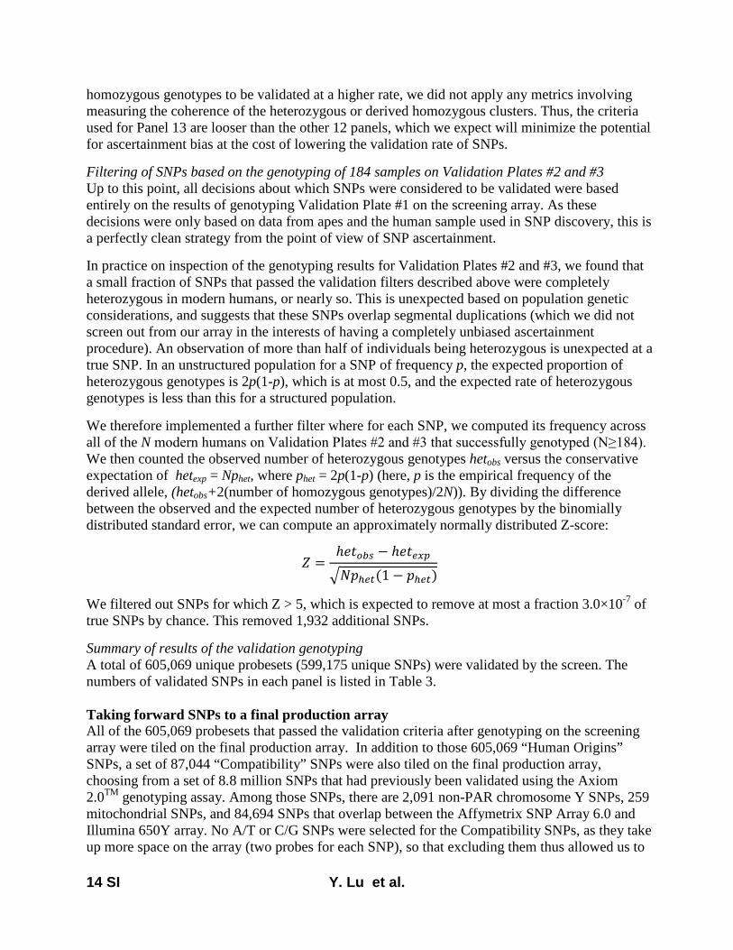
14 SI Y. Lu et al.

homozygous genotypes to be validated at a higher rate, we did not apply any metrics involving measuring the coherence of the heterozygous or derived homozygous clusters. Thus, the criteria used for Panel 13 are looser than the other 12 panels, which we expect will minimize the potential for ascertainment bias at the cost of lowering the validation rate of SNPs. Filtering of SNPs based on the genotyping of 184 samples on Validation Plates #2 and #3 Up to this point, all decisions about which SNPs were considered to be validated were based entirely on the results of genotyping Validation Plate #1 on the screening array. As these decisions were only based on data from apes and the human sample used in SNP discovery, this is a perfectly clean strategy from the point of view of SNP ascertainment. In practice on inspection of the genotyping results for Validation Plates #2 and #3, we found that a small fraction of SNPs that passed the validation filters described above were completely heterozygous in modern humans, or nearly so. This is unexpected based on population genetic considerations, and suggests that these SNPs overlap segmental duplications (which we did not screen out from our array in the interests of having a completely unbiased ascertainment procedure). An observation of more than half of individuals being heterozygous is unexpected at a true SNP. In an unstructured population for a SNP of frequency p, the expected proportion of heterozygous genotypes is 2p(1-p), which is at most 0.5, and the expected rate of heterozygous genotypes is less than this for a structured population. We therefore implemented a further filter where for each SNP, we computed its frequency across all of the N modern humans on Validation Plates #2 and #3 that successfully genotyped (N≥184). We then counted the observed number of heterozygous genotypes hetobs versus the conservative expectation of hetexp = Nphet, where phet = 2p(1-p) (here, p is the empirical frequency of the derived allele, (hetobs+2(number of homozygous genotypes)/2N)). By dividing the difference between the observed and the expected number of heterozygous genotypes by the binomially distributed standard error, we can compute an approximately normally distributed Z-score:

𝑍 =ℎ𝑒𝑡𝑜𝑏𝑠 − ℎ𝑒𝑡𝑒𝑥𝑝�𝑁𝑝ℎ𝑒𝑡(1 − 𝑝ℎ𝑒𝑡)

We filtered out SNPs for which Z > 5, which is expected to remove at most a fraction 3.0×10-7 of true SNPs by chance. This removed 1,932 additional SNPs. Summary of results of the validation genotyping A total of 605,069 unique probesets (599,175 unique SNPs) were validated by the screen. The numbers of validated SNPs in each panel is listed in Table 3. Taking forward SNPs to a final production array All of the 605,069 probesets that passed the validation criteria after genotyping on the screening array were tiled on the final production array. In addition to those 605,069 “Human Origins” SNPs, a set of 87,044 “Compatibility” SNPs were also tiled on the final production array, choosing from a set of 8.8 million SNPs that had previously been validated using the Axiom 2.0TM genotyping assay. Among those SNPs, there are 2,091 non-PAR chromosome Y SNPs, 259 mitochondrial SNPs, and 84,694 SNPs that overlap between the Affymetrix SNP Array 6.0 and Illumina 650Y array. No A/T or C/G SNPs were selected for the Compatibility SNPs, as they take up more space on the array (two probes for each SNP), so that excluding them thus allowed us to

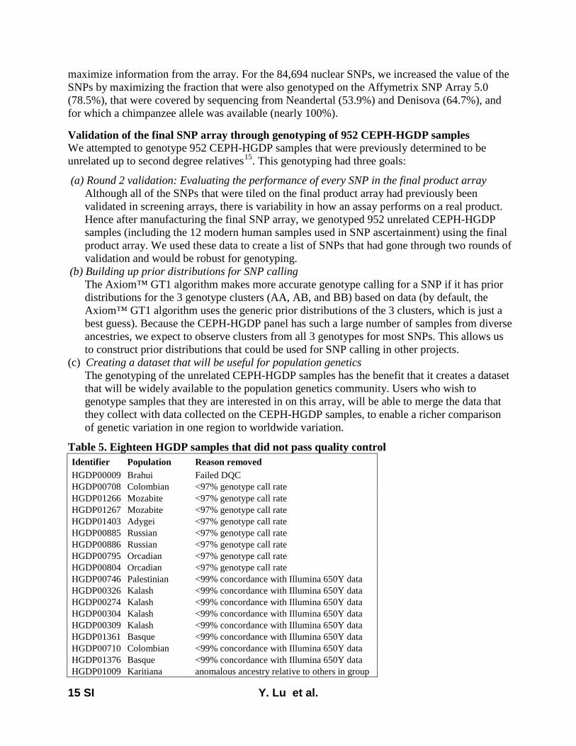
15 SI Y. Lu et al.

maximize information from the array. For the 84,694 nuclear SNPs, we increased the value of the SNPs by maximizing the fraction that were also genotyped on the Affymetrix SNP Array 5.0 (78.5%), that were covered by sequencing from Neandertal (53.9%) and Denisova (64.7%), and for which a chimpanzee allele was available (nearly 100%).

Validation of the final SNP array through genotyping of 952 CEPH-HGDP samples We attempted to genotype 952 CEPH-HGDP samples that were previously determined to be unrelated up to second degree relatives15. This genotyping had three goals:

(a) Round 2 validation: Evaluating the performance of every SNP in the final product array Although all of the SNPs that were tiled on the final product array had previously been validated in screening arrays, there is variability in how an assay performs on a real product. Hence after manufacturing the final SNP array, we genotyped 952 unrelated CEPH-HGDP samples (including the 12 modern human samples used in SNP ascertainment) using the final product array. We used these data to create a list of SNPs that had gone through two rounds of validation and would be robust for genotyping.

(b) Building up prior distributions for SNP calling The Axiom™ GT1 algorithm makes more accurate genotype calling for a SNP if it has prior distributions for the 3 genotype clusters (AA, AB, and BB) based on data (by default, the Axiom™ GT1 algorithm uses the generic prior distributions of the 3 clusters, which is just a best guess). Because the CEPH-HGDP panel has such a large number of samples from diverse ancestries, we expect to observe clusters from all 3 genotypes for most SNPs. This allows us to construct prior distributions that could be used for SNP calling in other projects.

(c) Creating a dataset that will be useful for population genetics The genotyping of the unrelated CEPH-HGDP samples has the benefit that it creates a dataset that will be widely available to the population genetics community. Users who wish to genotype samples that they are interested in on this array, will be able to merge the data that they collect with data collected on the CEPH-HGDP samples, to enable a richer comparison of genetic variation in one region to worldwide variation.

Table 5. Eighteen HGDP samples that did not pass quality control Identifier Population Reason removed HGDP00009 Brahui Failed DQC HGDP00708 Colombian <97% genotype call rate HGDP01266 Mozabite <97% genotype call rate HGDP01267 Mozabite <97% genotype call rate HGDP01403 Adygei <97% genotype call rate HGDP00885 Russian <97% genotype call rate HGDP00886 Russian <97% genotype call rate HGDP00795 Orcadian <97% genotype call rate HGDP00804 Orcadian <97% genotype call rate HGDP00746 Palestinian <99% concordance with Illumina 650Y data HGDP00326 Kalash <99% concordance with Illumina 650Y data HGDP00274 Kalash <99% concordance with Illumina 650Y data HGDP00304 Kalash <99% concordance with Illumina 650Y data HGDP00309 Kalash <99% concordance with Illumina 650Y data HGDP01361 Basque <99% concordance with Illumina 650Y data HGDP00710 Colombian <99% concordance with Illumina 650Y data HGDP01376 Basque <99% concordance with Illumina 650Y data HGDP01009 Karitiana anomalous ancestry relative to others in group

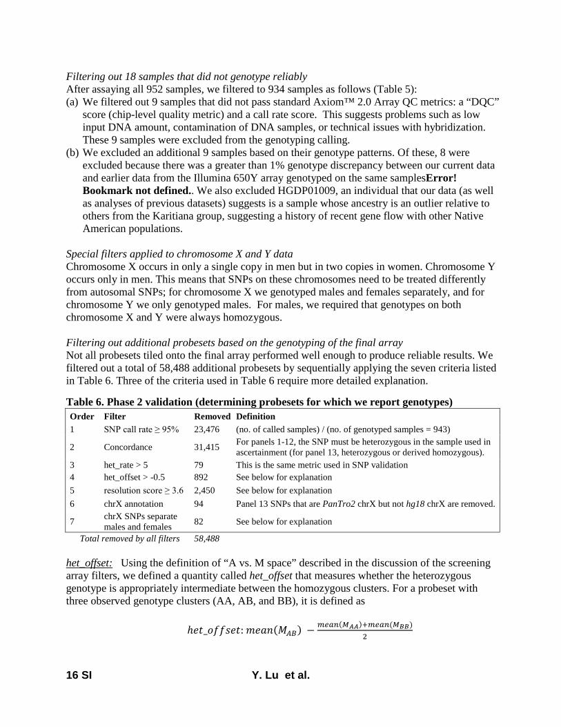
16 SI Y. Lu et al.

Filtering out 18 samples that did not genotype reliably After assaying all 952 samples, we filtered to 934 samples as follows (Table 5): (a) We filtered out 9 samples that did not pass standard Axiom™ 2.0 Array QC metrics: a “DQC”

score (chip-level quality metric) and a call rate score. This suggests problems such as low input DNA amount, contamination of DNA samples, or technical issues with hybridization. These 9 samples were excluded from the genotyping calling.

(b) We excluded an additional 9 samples based on their genotype patterns. Of these, 8 were excluded because there was a greater than 1% genotype discrepancy between our current data and earlier data from the Illumina 650Y array genotyped on the same samplesError! Bookmark not defined.. We also excluded HGDP01009, an individual that our data (as well as analyses of previous datasets) suggests is a sample whose ancestry is an outlier relative to others from the Karitiana group, suggesting a history of recent gene flow with other Native American populations.

Special filters applied to chromosome X and Y data Chromosome X occurs in only a single copy in men but in two copies in women. Chromosome Y occurs only in men. This means that SNPs on these chromosomes need to be treated differently from autosomal SNPs; for chromosome X we genotyped males and females separately, and for chromosome Y we only genotyped males. For males, we required that genotypes on both chromosome X and Y were always homozygous. Filtering out additional probesets based on the genotyping of the final array Not all probesets tiled onto the final array performed well enough to produce reliable results. We filtered out a total of 58,488 additional probesets by sequentially applying the seven criteria listed in Table 6. Three of the criteria used in Table 6 require more detailed explanation. Table 6. Phase 2 validation (determining probesets for which we report genotypes) Order Filter Removed Definition 1 SNP call rate ≥ 95% 23,476 (no. of called samples) / (no. of genotyped samples = 943)

2 Concordance 31,415 For panels 1-12, the SNP must be heterozygous in the sample used in ascertainment (for panel 13, heterozygous or derived homozygous).

3 het_rate > 5 79 This is the same metric used in SNP validation 4 het_offset > -0.5 892 See below for explanation 5 resolution score ≥ 3.6 2,450 See below for explanation 6 chrX annotation 94 Panel 13 SNPs that are PanTro2 chrX but not hg18 chrX are removed.

7 chrX SNPs separate males and females 82 See below for explanation

Total removed by all filters 58,488 het_offset: Using the definition of “A vs. M space” described in the discussion of the screening array filters, we defined a quantity called het_offset that measures whether the heterozygous genotype is appropriately intermediate between the homozygous clusters. For a probeset with three observed genotype clusters (AA, AB, and BB), it is defined as

ℎ𝑒𝑡_𝑜𝑓𝑓𝑠𝑒𝑡: 𝑚𝑒𝑎𝑛(𝑀𝐴𝐵) − 𝑚𝑒𝑎𝑛(𝑀𝐴𝐴)+𝑚𝑒𝑎𝑛(𝑀𝐵𝐵)2

17 SI Y. Lu et al.

For a probeset with one observed homozygous and one heterozygous cluster, it is defined as:

ℎ𝑒𝑡_𝑜𝑓𝑓𝑠𝑒𝑡: 𝑚𝑒𝑎𝑛(𝑀𝐴𝐵) −𝑚𝑒𝑎𝑛�𝑀𝐴𝐴|𝐵𝐵�

For other situations, het_offset is not used as a filter. resolution score: This is again defined in the M space of the “A vs M space”, and it measures how well the heterozygous cluster separates from the homozygous cluster(s). We define: resolution = 𝑎𝑏𝑠(𝑚𝑒𝑎𝑛(𝑀ℎ𝑜𝑚𝑜)− 𝑚𝑒𝑎𝑛(𝑀ℎ𝑒𝑡𝑒𝑟𝑜))

𝑠𝑑(𝑀ℎ𝑜𝑚𝑜)+𝑠𝑑(𝑀ℎ𝑒𝑡𝑒𝑟𝑜) × 2

For a probeset with three observed genotype clusters (AA, AB, and BB), the resolution score is defined as: min(𝑟𝑒𝑠𝑜𝑙𝑢𝑡𝑖𝑜𝑛𝐴𝐴−𝐴𝐵, 𝑟𝑒𝑠𝑜𝑙𝑢𝑡𝑖𝑜𝑛𝐵𝐵−𝐴𝐵). For a probeset with one observed homozygous cluster and one observed heterozygous cluster, the resolution score is the resolution between two clusters. For other situations, the resolution score is NA. chromosome X SNPs separate males and females: It was found that for some chromosome X SNPs, female samples and male samples formed distinct genotype clusters. Such cases most likely are not real chromosome X SNPs. One possible explanation for this pattern is SNPs derived from fixed differences between homologous chromosome X and chromosome Y sequences15,16. We removed chromosome X SNPs that meet all of the following criteria

1. All called male samples have the same genotype call 2. Greater than 85% of called female samples have the same genotype call and there are at

most 2 different called genotypes for females 3. The distance between the male genotype cluster center and the major female genotype

cluster center is at least 0.8 units in the M genotype clustering space.

The number of final validated SNPs is given in the final column of Table 7, and this is the set of SNPs for which we publically released data for 934 unrelated CEPH-HGDP samples on August 12, 2011. Table 7 summarizes the SNPs on the final product array. Table 7. Summary of SNPs in the final array Category number of probesets number of SNPs Human Origins 546,581 542,399 Chromosome Y 2,091 2,091 Mitochondrial DNA 259 259 Compatibility 84,694 84,694 Total 633,625 629,443 Upon commercial release of the array, Affymetrix is planning to release user-friendly software that will facilitate SNP calling using each of the ascertainment panels. Users who are interested in any particular ascertainment will open up one of 14 available folders of files (the first 13 corresponding to the SNPs in each ascertainment, and the 14th corresponding to all SNPs together). Users will then be able to use that folder (which will include ascertainment-panel specific priors) to call genotypes relevant to any given ascertainment panel.

18 SI Y. Lu et al.

The genotyping data on the 934 unrelated CEPH-HGDP samples that we collected as part of this project has been made freely available without restriction to the community by depositing the data into the CEPH-HGDP database on August 12, 2011 (ftp://ftp.cephb.fr/hgdp_supp10/). There are no restrictions on using these data and publishing papers based on these data. In addition to the dataset of 934 CEPH-HGDP samples that we released on August 12, 2011, we have also carried out further filtering to create a dataset of 828 samples that might be more useful for some population genetic analyses. This dataset, which is the one that we used for the analyses of population history reported in the present paper, is available for downloading from the Reich laboratory website (http://genetics.med.harvard.edu/reich/Reich_Lab/Welcome.html). To generate this dataset, we started with the dataset that was released to the CEPH-HGDP website on August 12, 2011, and then carried out population-specific Principal Component Analysis to identify individual samples that are outliers with respect to their own populations (consistent with admixture with other populations without the last few generation). These individuals were then filtered out of the dataset, allowing us to analyze data from a homogeneous population sample. Table 8 lists the number of samples from each population before and after the filtering. Table 8. Number of CEPH-HGDP samples in each of the two datasets reported here

Population Region Aug. 12

2011 Further filtering Population Region

Aug. 12 2011

Further filtering

BantuKenya Africa 11 10 Adygei West Eurasia 17 15 BantuSouthAfrica Africa 8 6 Basque West Eurasia 22 20 BiakaPygmy Africa 23 20 Bedouin West Eurasia 46 38 Mandenka Africa 22 20 Druze West Eurasia 42 32 Mbuti* Africa 13 12 French* West Eurasia 28 27 Mozabite Africa 27 25 Italian West Eurasia 13 11 San* Africa 6 5 Orcadian West Eurasia 13 13 Yoruba* Africa 22 22 Palestinian West Eurasia 45 34 Cambodian* East Asia 10 10 Russian West Eurasia 23 22 Dai East Asia 10 10 Sardinian* West Eurasia 28 27 Daur East Asia 9 7 Tuscan West Eurasia 8 7 Han* East Asia 34 33 Balochi South Asia 24 21 Han-NChina East Asia 10 10 Brahui South Asia 24 22 Hezhen East Asia 9 9 Burusho South Asia 25 24 Japanese East Asia 29 28 Hazara South Asia 22 17 Lahu East Asia 8 7 Kalash South Asia 19 18 Miao East Asia 10 10 Makrani South Asia 25 22 Mongola* East Asia 10 8 Pathan South Asia 24 22 Naxi East Asia 9 7 Sindhi South Asia 24 22 Oroqen East Asia 9 8 Colombian America 5 4 She East Asia 10 10 Karitiana* America 13 8 Tu East Asia 10 9 Maya America 21 18 Tujia East Asia 10 9 Pima America 14 11 Uygur East Asia 10 9 Surui America 8 6 Xibo East Asia 9 7 Melanesian* Oceania 11 9 Yakut East Asia 25 23 Papuan* Oceania 17 14 Yi East Asia 10 10

* Indicates a population used in SNP ascertainment. Analysis of data from these populations should remove the individual used in SNP discovery, as they have highly biased SNP genotypes (all heterozygotes) relative to others in the same group.

19 SI Y. Lu et al.

References

1 Rosenberg NA, Mahajan S, Ramachandran S, Zhao C, Pritchard JK, Feldman MW (2005) Clines, clusters, and the

effect of study design on the inference of human population structure. PLoS Genet. 1,e70. 2 Wang S et al. (2007) Genetic variation and population structure in native American. PLoS Genet. 3, e185. 3 Tishkoff SA et al. (2009) The genetic structure and history of Africans and African Americans. Science. 324, 1035-

44. 4 Friedlaender JS et al. (2008) The genetic structure of Pacific Islanders. PLoS Genet. 4, e19. 5 Rosenberg NA et al. (2006) Low levels of genetic divergence across geographically and linguistically diverse

populations from India. PLoS Genet. 2, e215. 6 Keinan A, Mullikin JC, Patterson N, Reich D (2007) Measurement of the human allele frequency spectrum

demonstrates greater genetic drift in East Asians than Europeans. Nature Genetics 39, 1251-1255 7 Reich D, Green RE, Kircher M, Krause J, Patterson N, Durand EY, Viola B, Briggs AW, Stenzel U, Johnson PLF,

Maricic T, Good JM, Marques-Bonet T, Alkan C, Fu Q, Mallick S, Li H, Meyer M, Eichler EE, Stoneking M, Richards M, Talamo S, Shunkov MV, Derevianko AP, Hublin JJ, Kelso J, Slatkin M & Pääbo S (2010) Genetic history of an archaic hominin group from Denisova Cave in Siberia. Nature 468, 1053-1060.

8 Li JZ et al. (2008) Worldwide human relationships inferred from genome-wide patterns of variation. Science 319, 1100-4. 9 Green RE et al. (2010) A draft sequence of the Neandertal genome. Science 328, 710-722. 10 Cann HM et al. (2002) A human genome diversity cell line panel. Science 296, 261-2. 11 Affymetrix Power Tools: http://www.affymetrix.com/partners_programs/programs/developer/tools/powertools.affx 12 Genotyping Console:

http://www.affymetrix.com/browse/level_seven_software_products_only.jsp?productId=131535&categoryId=35625#1_1

13 Single-sample analysis methodology for the DMET™ Plus Premier Pack - this white paper also applies to the Axiom GT1 genotyping algorithm. http://www.affymetrix.com/support/technical/whitepapers/dmet_plus_algorithm_whitepaperv1.pdf (pdf, 292 KB)

14 BRLMM-P: a Genotype Calling Method for the SNP 5.0 Array http://www.affymetrix.com/support/technical/whitepapers/brlmmp_whitepaper.pdf (pdf, 163 KB)

15 Rosenberg NA (2006) Standardized subsets of the HGDP-CEPH Human Genome Diversity Cell Line Panel, accounting for atypical and duplicated samples and pairs of close relatives. Ann Hum Genet 70, 841-7.

16 Ross MT et al. (2005) The DNA sequence of the human X chromosome. Nature, 434,325-337