Embed Size (px)
Citation preview
Ann. Henri Poincare Online Firstc© 2013 Springer BaselDOI 10.1007/s00023-013-0287-z Annales Henri Poincare
Anderson’s Orthogonality Catastrophefor One-Dimensional Systems
Heinrich Kuttler, Peter Otte and Wolfgang Spitzer
Abstract. The overlap, DN , between the ground state of N free fermi-ons and the ground state of N fermions in an external potential in onespatial dimension is given by a generalized Gram determinant. An upperbound is DN ≤ exp(−IN ) with the so-called Anderson integral IN . Weprove, provided the external potential satisfies some conditions, that inthe thermodynamic limit IN = γ ln N + O(1) as N → ∞. The coefficientγ > 0 is given in terms of the transmission coefficient of the one-particlescattering matrix. We obtain a similar lower bound on DN concludingthat CN−γ ≤ DN ≤ CN−γ with constants C, C, and γ. In particu-lar, DN → 0 as N → ∞ which is known as Anderson’s orthogonalitycatastrophe.
1. Introduction
In 1967, Anderson [4] studied the transition probability between the groundstate of N free fermions and the ground state of N fermions subject to anexterior (radially symmetric) potential in R3. Interestingly, he found that thisprobability decays like N−γ with some explicit γ > 0 (in terms of phase shiftsof the potential) as N → ∞. Here, we give a rigorous analysis of this so-calledorthogonality catastrophe for one-dimensional systems.
To begin with, let us briefly sketch the many-particle problem underlyingour considerations. The state space of N fermions is the N -fold anti-symmetrictensor product
HN := H ∧ · · · ∧ H︸ ︷︷ ︸
N−times
This work was supported by the research network SFB TR 12—‘Symmetries and Universalityin Mesoscopic Systems’ of the German Research Foundation (DFG).
H. Kuttler et al. Ann. Henri Poincare
of some one-particle space H (e.g., H = L2(Ω)⊗Cs, Ω ⊂ Rd, s, d ∈ N) where aone-particle Hamilton operator H : dom(H) → H is defined. Since we assumeour particles to not interact the corresponding operator HN on HN is simplya sum
HN := H ∧ 1 ∧ · · · ∧ 1 + · · · + 1 ∧ · · · ∧ 1 ∧H.If H has a discrete spectrum consisting of (simple) eigenvalues λ1 < λ2 < · · ·with corresponding eigenvectors ϕ1, ϕ2, . . . one can easily construct the anal-ogous N -particle quantities. In particular, the ground state ϕN is a Slaterdeterminant and the eigenvalue λN a sum, i.e.,
ϕN = ϕ1 ∧ · · · ∧ ϕN , λN = λ1 + · · · + λN .
Note that the definition of the wedge product contains the factor (N !)−1/2,whereby the product of normalized vectors automatically becomes normalized.Let HV := H + V be a second operator on H with (simple) eigenvalues μ1 <μ2 < · · · and eigenvectors ψ1, ψ2, . . .. The operator HN
V is defined analogouslyto HN and thus the new ground state and its energy are
ψN = ψ1 ∧ · · · ∧ ψN , μN = μ1 + · · · + μN .
The transition probability, DN , studied by Anderson is given through thescalar product
DN := |(ϕN , ψN )|2 = |det((ϕj , ψk))j,k=1,...,N |2. (1.1)
It can be estimated (see 5.21) as
DN ≤ e−IN , IN :=N∑
j=1
∞∑
k=N+1
|(ϕj , ψk)|2. (1.2)
Here, IN is the so-called ‘Anderson integral’ which is the object of our maininterest. The asymptotics we wish to analyze involves a second parameter Lreflecting the system length so that H = HL = L2([−L,L]d) is the Hilbertspace of (spin-less) fermions confined to the box [−L,L]d. Therefore, we workwith a sequence of Hilbert spaces HL and ground states ϕN = ϕN
L , ψN =ψN
L with L > 0. In the thermodynamic limit we let N,L → ∞ with theparticle density N/(2L)d being (asymptotically) kept fixed. Our main result(Theorem 5.3, Corollary 5.4) is an asymptotic formula for IN,L in d = 1:
Theorem. Let the potential V ∈ L1(R) satisfy in addition X2V ∈ L1(R) andV,X3V ∈ L∞(R) where for short XnV : x → xnV (x), n ∈ N. Choose N andL such that the Fermi energy
ν =[
π
2L
(
N +12
)]2
is constant and V is small compared to the particle density, that is, 4‖V ‖1 <√ν. Then, the Anderson integral has the leading asymptotics
IN,L = γ(ν) lnN +O(1), N, L → ∞,
Anderson’s Orthogonality Catastrophe
with
γ(ν) =1π2
(1 − Re t(√ν))
where t(√ν) is the transmission coefficient at energy ν (cf. [5]).
Scattering theory tells us (see [5,13]) that usually γ(ν) > 0 the asymptot-ics otherwise being useless. We derive also a lower bound on DN which is basedupon an estimate for the spectral projections of H and HV in Theorem 5.5which assumes that V satisfies an additional smallness assumption. Then, thetransition probability behaves precisely as (Corollary 5.6)
CN−γ(ν) ≤ DN,L ≤ CN−γ(ν), N, L → ∞.
Here, γ(ν) > 0 can be derived from γ(ν).The main ingredient of the theorem’s proof is an integral formula for IN,L
(Proposition 2.1), which holds true under rather general conditions. It restsessentially upon the Riesz integral formula for spectral projections and Krein’sresolvent formula. In order to adapt it to Schrodinger operators we derive aresolvent formula involving abstract differentiation and multiplication opera-tors (Proposition 2.2). Via this formula, a sequence of scalar functions comesinto play which tends at least informally to a Dirac delta function. This is madeprecise in Sects. 3.3 and 4, hence the name delta-term and delta-estimate. Thesingularity represented by the delta sequence reflects in a way the singulartransition from a discrete spectrum to a continuous spectrum as L → ∞.
Our method requires a rather detailed and precise knowledge of the freeDirichlet problem, in particular of the resolvent. Almost everything one needsto know about the perturbed problem, however, can be read off from theso-called T-operator. The perturbed eigenvalues do not enter in the actualasymptotic analysis. We only need to make sure that the number of perturbedeigenvalues below some fixed (Fermi) energy is asymptotically the same forlarge N as for the free problem (see Proposition 3.10). This is related to thespectral shift function (see [11] for potentials with compact support). Inter-estingly, a lot of work has been done to derive asymptotic formulae for theperturbed eigenvalues at large energies. Except for [2], we are not aware ofstudies that include also the dependence on L as well.
Gebert et al. [8] using different methods have recently established a rig-orous lower bound
IN,L ≥ γ′ lnN, N,L → ∞,
in any dimension (even with a periodic background potential but with posi-tive and compactly supported exterior potential V ). Remarkably, their value γ′
agrees with Anderson’s prediction. In our framework, the expression for γ thatat first came out from Theorem 5.3 is rather implicit. Only after some computa-tion could we confirm that γ = γ′, Corollary 5.4. Thus, one can reasonably con-jecture that γ′ lnN is indeed the exact leading asymptotics in any dimension.
Anderson’s orthogonality catastrophe has attracted a lot of interest insolid-state physics since its discovery. In [4], Anderson mentions applicationsof this orthogonality catastrophe to important physical phenomena such as
H. Kuttler et al. Ann. Henri Poincare
the Mossbauer effect, Kondo effect, and to anomalies in impurity resistance. Anewer account on these phenomena and its derivation was described by Lloyd[12] and Affleck [1].
Starting with Anderson [3], it has been attempted to determine theasymptotics of the determinant DN itself. Rivier and Simanek [20] used theadiabatic theorem to express DN through the solution of a Wiener–Hopf equa-tion. However, they could not deal satisfactorily with certain limit proceduresunderlying the method. This was improved upon by Hamann [9] who, likewise,could treat the thermodynamic limit only informally. A clarification of thatmethod can be found in [17]. Recent numerical investigations have been carriedout by Weichselbaum et al. [22], who also present some physical backgroundand refer to further reading. Though not being completely rigorous from amathematical point of view, those results indicate that DN decays faster withan exponent γdet different from both γ and γ.
Frank et al. [7, Eq. 11] considered the related problem of proving alower bound to the energy difference—in our notation below tr(HV Π−HP )—directly in the thermodynamic limit in terms of semi-classical quantities.
2. Representation of the Anderson Integral
Let H be a Hilbert space with scalar product (·, ·), which is anti-linear inthe first component and linear in the second component and let ‖ · ‖ be thecorresponding vector norm. The induced operator norm will be denoted withthe same symbol ‖ · ‖. We consider a self-adjoint operator H : dom(H) → H,dom(H) ⊂ H, and a bounded operator V : H → H. Then, HV = H + V isself-adjoint as well with dom(HV ) = dom(H). We denote by σ(H) and σ(HV )the spectrum of H and HV , respectively, and by
R(z) := (z1 −H)−1, z ∈ C\σ(H), RV (z) := (z1 −HV )−1, z ∈ C\σ(HV )(2.1)
their resolvents. From spectral theory we know
‖R(z)‖ =1
dist(z, σ(H)), ‖RV (z)‖ =
1dist(z, σ(HV ))
. (2.2)
We borrow some notation from scattering theory (see e.g., [21, 3.6]). Note, thatfor z /∈ σ(H) the operator (1 − V R(z))−1 exists and is bounded if and onlyif z /∈ σ(HV ). The same holds true for (1 − R(z)V )−1. Hence, the so-calledtransition operator or T-operator
T (z) := (1 − V R(z))−1V = V (1 −R(z)V )−1 (2.3)
exists for z ∈ C\(σ(H) ∪ σ(HV )) with
‖T (z)‖ ≤ dist(z, σ(H))dist(z, σ(HV ))
‖V ‖ (2.4)
and is analytic there as a function of z. Krein’s resolvent formula
RV (z) −R(z) = R(z)T (z)R(z) (2.5)
Anderson’s Orthogonality Catastrophe
relates the resolvents R(z) and RV (z) with each other whenever the T-operatorexists. The operator V plays an important role via its modified polar decom-position
V =√
|V |J√
|V |, J∗ = J, J2 = 1, ‖J‖ = 1, (2.6)
which is obvious for the multiplication operators used below. Like in scatteringtheory it is advantageous to look at operators relative to V . More precisely,we will use (cf. [21, 3.6.1, 1])
√
|V |R(z)√
|V |, Ω(z) :=(
1 −√
|V |R(z)√
|V |J)−1
(2.7)
with the sandwiched resolvent being called Birman–Schwinger operator. Notethe relation
T (z) =√
|V |JΩ(z)√
|V |. (2.8)
Obviously, the Birman–Schwinger operator exists and is bounded for z ∈C\σ(H). For Ω(z) to exist as a bounded operator it is required that z /∈C\(σ(H) ∪ σ(HV )). The converse is true, too. That is to say, if z /∈ σ(H) andΩ(z) exists and is bounded then z /∈ σ(HV ). In order to see this one first showsthat 1 − R(z)V is injective and has dense range and, in a second step, thatthe range is closed.
2.1. Operators with a Common Spectral Gap
Riesz’s integral formula yields a handy expression for the Anderson integralwhen the operators H and HV have a common spectral gap. That is to saytheir spectra can be written as
σ(H) = σ1(H) ∪ σ2(H), σ(HV ) = σ1(HV ) ∪ σ2(HV ) (2.9)
such that there is a closed contour Γ ⊂ C with each σ1 being inside and eachσ2 outside of Γ. Let P be the spectral projection of H belonging to σ1(H) andlet Π be defined likewise for HV . The Anderson integral in question is
I := tr [P (1 − Π)] . (2.10)
In our application P is trace class and hence 0 ≤ I < ∞. The Riesz formulareads
P =1
2πi
∫
Γ
R(z) dz, Π =1
2πi
∫
Γ
RV (z) dz. (2.11)
Note that both integrals have the same Γ from above. For our purposes, aninfinite contour is more appropriate. In particular, due to the special form ofthe free Green function (see 3.12) a parabola will do best. Given that ν willbe the Fermi energy (3.4) from Sect. 3 onward we assume ν > 0 for simplicity.
Proposition 2.1. Let P be trace class. We assume the sets σ1,2 in (2.9) tosatisfy
supσ1(H) < ν < inf σ2(H), supσ1(HV ) < ν < inf σ2(HV ) (2.12)
H. Kuttler et al. Ann. Henri Poincare
with some ν ∈ R, ν > 0, and define the parabola Γν :={z=(√ν+is)2 | s∈R}.
Then, the difference of the spectral projections has the representation
Π − P =1
2πi
∫
Γν
R(z)T (z)R(z) dz (2.13)
and the Anderson integral (2.10) can be written as
I =1
2πi
∫
Γν
tr[
PR(z)T (z)R(z)2T (z)]
dz. (2.14)
Proof. By Riesz’s and Krein’s formulae, (2.11) and (2.5),
Π − P =1
2πi
∫
Γ
(RV (z) −R(z)) dz =1
2πi
∫
Γ
R(z)T (z)R(z) dz (2.15)
with the closed contour Γ used in (2.9). For the Anderson integral noteP (Π − 1) = P (Π − P ) which allows us to use (2.15). Since P is trace classand the other operators are bounded, we may take the trace. Using the cycliccommutativity we obtain
I = − 12πi
∫
Γ
tr [PR(z)T (z)R(z)] dz = − 12πi
∫
Γ
tr[
PR(z)2T (z)]
dz,
since P commutes with R(z). Recall that R(z) is differentiable in z ∈ C\σ(H)with R′(z) = −R(z)2. Since all functions involved are analytic for z ∈C\(σ(H) ∪ σ(HV )), we may integrate by parts,
I = − 12πi
∫
Γ
tr [PR(z)T ′(z)] dz =1
2πi
∫
Γ
tr[
PR(z)T (z)R(z)2T (z)]
dz.
(2.16)
By the estimates (2.2) and (2.4) the integrands in (2.15) and (2.16) decay fastenough at infinity so that we may bend the closed contour Γ into the parabolaΓν to obtain (2.13) and (2.14), respectively. �
The integral formula (2.14) for the Anderson integral was intentionallymade more complicated via integration by parts. For, in the application of thedelta-estimate to (2.14) it will be important to have the smooth cut-off factorPR(z) instead of just P .
2.2. Schrodinger-Type Operators
A typical Schrodinger operator is built from differentiation and multiplicationoperators. Let us introduce two operators ∇ and X satisfying
[∇,X] = 1. (2.17)
We assume ∇ : dom(∇) → H, dom(∇) ⊂ H, to be densely defined on H andX : H → H to be bounded such that X(dom(∇)) ⊂ dom(∇). Thus, (2.17)is meant to hold true on dom(∇). Self-adjointness of Schrodinger operatorsoften results from boundary conditions which usually lessen the domain of
Anderson’s Orthogonality Catastrophe
definition. Let −∇2 have a self-adjoint restriction H : dom(H) → H, i.e.,dom(H) ⊂ dom(∇2) and
H = −∇2 on dom(H). (2.18)
The resolvent of H,
R(z) = (z1 −H)−1, z ∈ C\σ(H)
is a well-defined and bounded operator with R(z) : H → dom(H). The latterimplies
(z1 + ∇2)R(z) = (z1 −H)R(z) = 1. (2.19)
In general, this equality fails to hold true when the order of terms is switchedas can be seen in Proposition 3.6. This is the reason why the following resolventformula gives non-trivial results.
Proposition 2.2. For operators ∇ and X as in (2.17) let us assume in additionX(dom(H)) ⊂ dom(H). Then, the decomposition
R(z)2 =1zR(z) − 1
2z[X∇, R(z)] +
1zD(z) =
12z
(R(z) − C(z)) +1zD(z)
(2.20)
holds true on dom(∇2) and for z ∈ C\σ(H). Here,
D(z) :=(
12X −R(z)∇
)
[∇, R(z)], C(z) := X∇R(z) −R(z)∇X. (2.21)
The operator D(z) is the so-called ‘delta-term’ and satisfies
(z1 + ∇2)D(z) = 0 (2.22)
on dom(∇2) and for z ∈ C\σ(H).
Proof. We start off from the elementary formula
R(z)2 =1zR(z) +
1zR(z)HR(z) (2.23)
and rewrite the last term. By the product rule the commutator in (2.20)becomes
[X∇, R(z)] = X[∇, R(z)] + [X,R(z)]∇. (2.24)
Formula (2.17) implies [∇2,X] = 2∇. By noting X(dom(H)) ⊂ dom(H) andR(z)(z1 −H) = 1 on dom(H) we obtain
[X,R(z)] = R(z)[z1 −H,X]R(z) = R(z)[∇2,X]R(z) = 2R(z)∇R(z).
Thus,
12[X,R(z)]∇ = R(z)∇R(z)∇ = R(z)∇2R(z) +R(z)∇[R(z),∇]
Recalling (2.18) we solve for R(z)HR(z), insert this into (2.23), and use (2.24).Then,
H. Kuttler et al. Ann. Henri Poincare
R(z)2 =1zR(z) − 1
2z[X,R(z)]∇ − 1
zR(z)∇[∇, R(z)]
=1zR(z) − 1
2z[X∇, R(z)] +
12zX[∇, R(z)] − 1
zR(z)∇[∇, R(z)].
With the definition (2.21) of D(z) this is the first equality in (2.20). The secondone follows by means of the commutation relation X∇ = −1 + ∇X. Finally,by (2.17)
(z1 + ∇2)(
12X −R(z)∇
)
=12X(z1 + ∇2).
Then,
(z1 + ∇2)[∇, R(z)] = ∇(z1 + ∇2)R(z) − (z1 + ∇2)R(z)∇ = 0
shows (2.22). �
Our motivation behind the resolvent formula (2.20) in Proposition 2.2 isthat it splits the integrand tr[PR(z)T (z)R(z)2T (z)] in the integral represen-tation of the Anderson integral, Proposition 2.1, into a sum of two terms. Thefirst term, tr[PR(z)T (z)(R(z) − C(z))T (z)], will be subdominant, i.e., O(1),as shown in Sect. 5.1, whereas the second term tr[PR(z)T (z)D(z)T (z)] is ofthe leading order lnN , see Sect. 5.2. The operator D(z) quantifies the differ-ence between the resolvent of the Laplace operator with and without Dirichletboundary conditions.
3. One-Dimensional Schrodinger Operators
We look into the special case of Schrodinger operators with Dirichlet boundaryconditions on the finite interval [−L,L]. Our Hilbert space then becomes H =L2[−L,L]. Actually, it ought to bear an index L as well as all operators definedon it and related quantities. However, since this dependence is ubiquitous wetacitly suppress it. In our concrete case,
∇ =ddx, (Xϕ)(x) = xϕ(x). (3.1)
The domain dom(∇) as well as dom(∇2) can be described with the aid ofSobolev spaces which we do not need in detail herein. One can show thatX(dom(∇)) ⊂ dom(∇). The operator H becomes
H = −∇2 = − d2
dx2on dom(H),
where dom(H) is dom(∇2) restricted by Dirichlet boundary conditions.Because of that we have X(dom(H)) ⊂ dom(H). The corresponding eigen-value problem reads
− ϕ′′ = λϕ, ϕ(−L) = 0 = ϕ(L). (3.2)
Anderson’s Orthogonality Catastrophe
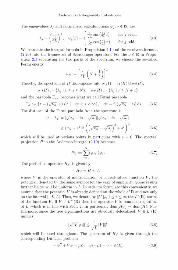
The eigenvalues λj and normalized eigenfunctions ϕj , j ∈ N, are
λj =(
πj
2L
)2
, ϕj(x) =
⎧
⎨
⎩
1√L
sin(
πj2Lx
)
for j even,1√L
cos(
πj2Lx
)
for j odd.(3.3)
We translate the integral formula in Proposition 2.1 and the resolvent formula(2.20) into the framework of Schrodinger operators. For the ν ∈ R in Propo-sition 2.1 separating the two parts of the spectrum, we choose the so-calledFermi energy
νN :=[
π
2L
(
N +12
)]2
. (3.4)
Thereby, the spectrum of H decomposes into σ(H) = σ1(H) ∪ σ2(H),
σ1(H) := {λj | 1 ≤ j ≤ N}, σ2(H) := {λj | j ≥ N + 1}and the parabola ΓνN
becomes what we call Fermi parabola
ΓN := {z = (√νN + is)2 | −∞ < s < ∞}, dz = 2i(
√νN + is) ds. (3.5)
The distance of the Fermi parabola from the spectrum is
|z − λj | = |√νN + is+√
λj ||√νN + is−√λj |
≥ (νN + s2)12
((√
νN −√λj
)2
+ s2) 1
2
, (3.6)
which will be used at various points in particular with s = 0. The spectralprojection P in the Anderson integral (2.10) becomes
PN :=N∑
j=1
(ϕj , ·)ϕj . (3.7)
The perturbed operator HV is given by
HV = H + V,
where V is the operator of multiplication by a real-valued function V , thepotential, denoted by the same symbol for the sake of simplicity. Some resultsfurther below will be uniform in L. In order to formulate this conveniently, weassume that the potential V is already defined on the whole of R and not onlyon the interval [−L,L]. Thus, we denote by ‖V ‖r, 1 ≤ r ≤ ∞ the Lr(R) normsof the function V . If V ∈ L∞(R) then the operator V is bounded regardlessof L, which is in line with Sect. 2. In particular, dom(HV ) = dom(H). Fur-thermore, since the free eigenfunctions are obviously delocalized, V ∈ L1(R)implies
‖√
|V |ϕj‖ ≤ 1√L
‖V ‖ 121 , (3.8)
which will be used throughout. The spectrum of HV is given through thecorresponding Dirichlet problem
− ψ′′ + V ψ = μψ, ψ(−L) = 0 = ψ(L). (3.9)
H. Kuttler et al. Ann. Henri Poincare
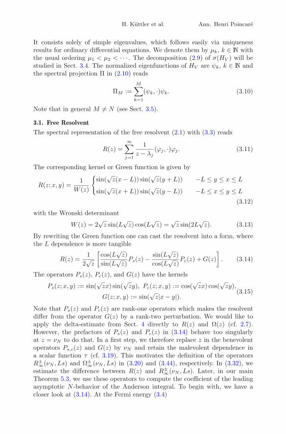
It consists solely of simple eigenvalues, which follows easily via uniquenessresults for ordinary differential equations. We denote them by μk, k ∈ N withthe usual ordering μ1 < μ2 < · · · . The decomposition (2.9) of σ(HV ) will bestudied in Sect. 3.4. The normalized eigenfunctions of HV are ψk, k ∈ N andthe spectral projection Π in (2.10) reads
ΠM :=M∑
k=1
(ψk, ·)ψk. (3.10)
Note that in general M �= N (see Sect. 3.5).
3.1. Free Resolvent
The spectral representation of the free resolvent (2.1) with (3.3) reads
R(z) =∞∑
j=1
1z − λj
(ϕj , ·)ϕj . (3.11)
The corresponding kernel or Green function is given by
R(z;x, y) =1
W (z)
{
sin(√z(x− L)) sin(
√z(y + L)) −L ≤ y ≤ x ≤ L
sin(√z(x+ L)) sin(
√z(y − L)) −L ≤ x ≤ y ≤ L
(3.12)
with the Wronski determinant
W (z) = 2√z sin(L
√z) cos(L
√z) =
√z sin(2L
√z). (3.13)
By rewriting the Green function one can cast the resolvent into a form, wherethe L dependence is more tangible
R(z) =1
2√z
[
cos(L√z)
sin(L√z)Ps(z) − sin(L
√z)
cos(L√z)Pc(z) +G(z)
]
. (3.14)
The operators Ps(z), Pc(z), and G(z) have the kernels
Ps(z;x, y) := sin(√zx) sin(
√zy), Pc(z;x, y) := cos(
√zx) cos(
√zy),
G(z;x, y) := sin(√z|x− y|). (3.15)
Note that Ps(z) and Pc(z) are rank-one operators which makes the resolventdiffer from the operator G(z) by a rank-two perturbation. We would like toapply the delta-estimate from Sect. 4 directly to R(z) and Ω(z) (cf. 2.7).However, the prefactors of Ps(z) and Pc(z) in (3.14) behave too singularlyat z = νN to do that. In a first step, we therefore replace z in the benevolentoperators Ps,c(z) and G(z) by νN and retain the malevolent dependence ina scalar function τ (cf. 3.19). This motivates the definition of the operatorsR±
∞(νN , Ls) and Ω±∞(νN , Ls) in (3.20) and (3.44), respectively. In (3.32), we
estimate the difference between R(z) and R±∞(νN , Ls). Later, in our main
Theorem 5.3, we use these operators to compute the coefficient of the leadingasymptotic N -behavior of the Anderson integral. To begin with, we have acloser look at (3.14). At the Fermi energy (3.4)
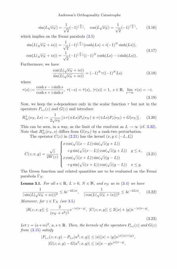
Anderson’s Orthogonality Catastrophe
sin(L√νN ) =
1√2(−1)� N
2 �, cos(L√νN ) =
1√2(−1)� N
2 , (3.16)
which implies on the Fermi parabola (3.5)
sin(L(√νN + is)) =
1√2(−1)� N
2 �(cosh(Ls) + i(−1)N sinh(Ls)),
cos(L(√νN + is)) =
1√2(−1)� N
2 �((−1)N cosh(Ls) − i sinh(Ls)).(3.17)
Furthermore, we havecos(L(
√νN + is))
sin(L(√νN + is))
= (−1)Nτ((−1)NLs) (3.18)
where
τ(s) :=cosh s− i sinh scosh s+ i sinh s
, τ(−s) = τ(s), |τ(s)| = 1, s ∈ R, lims→∞ τ(s) = −i.
(3.19)
Now, we keep the s-dependence only in the scalar function τ but not in theoperators Ps,c(z) and G(z) and introduce
R±∞(νN , Ls) :=
12√νN
[±τ(±Ls)Ps(νN ) ∓ τ(∓Ls)Pc(νN ) +G(νN )] . (3.20)
This can be seen, in a way, as the limit of the resolvent as L → ∞ (cf. 3.32).Note that R±
∞(νN , s) differs from G(νN ) by a rank-two perturbation.The operator C(z) in (2.21) has the kernel (x, y ∈ [−L,L])
C(z;x, y) =√z
2W (z)
⎧
⎪⎪⎪⎪⎪⎨
⎪⎪⎪⎪⎪⎩
x cos(√z(x− L)) sin(
√z(y + L))
+y sin(√z(x− L)) cos(
√z(y + L)) y ≤ x,
x cos(√z(x+ L)) sin(
√z(y − L))
+y sin(√z(x+ L)) cos(
√z(y − L)) x ≤ y.
(3.21)
The Green function and related quantities are to be evaluated on the Fermiparabola ΓN .
Lemma 3.1. For all s ∈ R, L > 0, N ∈ N, and νN as in (3.4) we have1
| sin(L(√νN + is))|2 ≤ 4e−2L|s|,
1| cos(L(
√νN + is))|2 ≤ 4e−2L|s|. (3.22)
Moreover, for z ∈ ΓN (see 3.5)
|R(z;x, y)| ≤ 2(νN + s2)
12e−|s||x−y|, |C(z;x, y)| ≤ 2(|x| + |y|)e−|s||x−y|.
(3.23)
Let z = (a+ is)2, a, s ∈ R. Then, the kernels of the operators Ps,c(z) and G(z)from (3.15) satisfy
|Ps,c(z;x, y) − Ps,c(a2;x, y)| ≤ |s|(|x| + |y|)e|s|(|x|+|y|),
|G(z;x, y) −G(a2;x, y)| ≤ |s||x− y|e|s||x−y|.
H. Kuttler et al. Ann. Henri Poincare
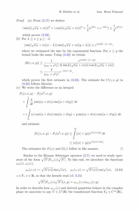
Proof. (a) From (3.17) we deduce
| sin(L(√νN + is))|2 = | cos(L(
√νN + is))|2 =
14(e2Ls + e−2Ls) ≥ 1
4e2L|s|
which proves (3.22).(b) For L ≥ x ≥ y ≥ −L
| sin((√νN + is)(x− L)) sin((
√νN + is)(y + L))| ≤ e|s|(2L−|x−y|),
where we estimated the sine by the exponential function. For x ≤ y thebound looks the same. Using (3.22) we obtain
|R(z;x, y)| ≤ 1(νN + s2)
12
e|s|(2L−|x−y|)
2| sin(L(√νN + is))|| cos(L(
√νN + is))|
≤ 2(νN + s2)
12e−|s||x−y|,
which proves the first estimate in (3.23). The estimate for C(z;x, y) in(3.23) follows likewise.
(c) We write the difference as an integral
Ps(z;x, y) − Ps(a2;x, y)
=
s∫
0
ddt
(sin((a+ it)x) sin((a+ it)y)) dt
= i
s∫
0
(x cos((a+ it)x) sin((a+ it)y) + y sin((a+ it)x) cos((a+ it)y)) dt,
and estimate
|Ps(z;x, y) − Ps(a2;x, y)| ≤|s|∫
0
(|x| + |y|)et(|x|+|y|) dt
≤ |s|(|x| + |y|)e|s|(|x|+|y|).
The estimates for Pc(z) and G(z) follow in like manner. �
Similar to the Birman–Schwinger operator (2.7), we need to study oper-ators of the form
√|V |Ps,c(z)√|V |. To this end, we introduce the functions
ωs(z), ωc(z),
ωs(z;x) :=√
|V (x)| sin(√zx), ωc(z, x) :=
√
|V (x)| cos(√zx), (3.24)
z ∈ C, x ∈ R, so that the kernels read (cf. 3.15)√
|V |Ps,c(z)√
|V |(x, y) = ωs,c(z;x)ωs,c(z; y).
In order to describe how ωs,c(z) and derived quantities behave in the complexplane we associate to any V ∈ L1(R) the transformed function VL ∈ C∞(R),
Anderson’s Orthogonality Catastrophe
VL(s) :=
L∫
−L
|V (x)|es|x| dx, s ∈ R. (3.25)
Its derivatives satisfy
0 ≤ V(p)L (0) ≤ V
(p)L (s), V
(p+q)L (0) ≤ Lp‖XqV ‖1,
V(p+q)L (s) ≤ Lp‖XqV ‖∞
L∫
−L
es|x| dx (3.26)
with p, q ∈ N0 provided that XqV ∈ L1(R) and XqV ∈ L∞(R), respectively.
Lemma 3.2. Let V ∈ L1(R) and z = (a+ is)2 with a, s ∈ R. Then,
‖ωs,c(z)‖ ≤ VL(2|s|) 12 , (3.27)
‖ωs,c(z) − ωs,c(a2)‖ ≤ |s|V (2)L (2|s|) 1
2 . (3.28)
Proof. In order to prove (3.27) we estimate
‖ωs(z)‖2 =
L∫
−L
|V (x)|| sin((a+ is)x)|2 dx ≤L∫
−L
|V (x)|e2|sx| dx.
For (3.28) we compute
‖ωs(z) − ωs(a2)‖2 =
L∫
−L
|V (x)| · | sin((a+ is)x) − sin(ax)|2 dx
and use the estimate
| sin((a+ is)x) − sin(ax)| = |ixs∫
0
cos((a+ it)x) dt| ≤ |x||s|e|sx|,
which yields (3.28). The estimates for ωc(z) follow in like manner. �
One could use Lemma 3.1 to study the norms of R(z) or G(z). However,the applications we have in mind require that to be done for the Birman–Schwinger (see 2.7) and suchlike operators (with
√|V | multiplied from leftand right).
Lemma 3.3. Let V ∈ L1(R) and z ∈ ΓN . Then, the Birman–Schwinger opera-tor satisfies
‖√
|V |R(z)√
|V |‖ ≤ 4√νN + s2
‖V ‖1. (3.29)
If X2V ∈ L1(R) with X as in (3.1) the operator C(z) from (3.21) satisfies
‖√
|V |C(z)√
|V |‖ ≤ 8‖X2V ‖ 121 ‖V ‖ 1
21 . (3.30)
Furthermore, for the operators G(νN ) from (3.15) and R±∞(νN , s) from (3.20)
we have
H. Kuttler et al. Ann. Henri Poincare
‖√
|V |G(νN )√
|V |‖ ≤ ‖V ‖1, ‖√
|V |R±∞(νN , s)
√
|V |‖ ≤ 32√νN
‖V ‖1. (3.31)
Finally,
‖√
|V |(R∞(νN , Ls) −R((√νN + is)2))
√
|V |‖≤ 3
2νNVL(0)|s| +
3√νN
|s|V (2)L (2|s|) 1
2VL(2|s|) 12 (3.32)
where R∞ stands for R+∞, R−
∞ depending on whether N in νN is even or odd.
Proof. Let the kernel W (x, y) of the integral operator W be bounded by
|W (x, y)| ≤ |W1(x)f(x, y)W2(x)|where W1,W2 ∈ L2(R) and f ∈ L∞(R2). By the Cauchy–Schwarz inequality
‖Wϕ‖2 ≤L∫
−L
|W1(x)|2L∫
−L
|f(x, y)W2(y)|2 dy dx ‖ϕ‖2
≤ ‖f‖2∞‖W1‖2
2 ‖W2‖22 ‖ϕ‖2
for ϕ ∈ L2[−L,L]. The norms of W1,2 and f pertain to R and R2, respectively.Hence
‖W‖ ≤ ‖f‖∞ ‖W1‖2 ‖W2‖2.
In order to prove (3.29), we can take W1,2 =√|V | and f ≡ 1 because of
(3.23). By the same estimate, we can prove (3.30) by using W1 = X√|V |,
W2 =√|V |, f ≡ 1 and W1 =
√|V |, W2 = X√|V |, f ≡ 1.
Because of the obvious bound |G(νN ;x, y)| ≤ 1 (cf. 3.15), we obtain
‖√
|V |G(νN )√
|V |‖ ≤ VL(0),
which proves (3.31) for G(νN ) via (3.26). Using this and (3.27) along with|τ(Ls)| = 1 we obtain for all s ∈ R
2√νN‖
√
|V |R±∞(νN , s)
√
|V |‖≤ ‖√
|V |Ps(νN )√
|V |‖ + ‖√
|V |Pc(νN )√
|V |‖ + ‖√
|V |G(νN )√
|V |‖≤ 3VL(0),
which gives (3.31) for R±∞(νN , s) via (3.26).
In order to prove (3.32) we use the kernel estimates in Lemma 3.1 andobtain
‖√
|V |(Ps,c(z) − Ps,c(νN ))√
|V |‖ ≤ 2|s|V (2)L (2s)
12VL(2|s|) 1
2 ,
‖√
|V |(G(z) −G(νN ))√
|V |‖ ≤ 2|s|V (2)L (2|s|) 1
2VL(2|s|) 12 ,
which would also be true for other real values than νN but that is not neededhere. Using (3.14) and |τ(Ls)| = 1 we obtain
Anderson’s Orthogonality Catastrophe
2‖(R∞(νN , Ls) −R(z))‖≤ 1√
νN + s2(‖Ps(νN ) − Ps(z)‖ + ‖Pc(νN ) − Pc(z)‖ + ‖G(νN ) −G(z)‖)
+∣
∣
1√νN
− 1√νN + is
∣
∣ (‖Ps(νN )‖ + ‖Pc(νN )‖ + ‖G(νN )‖) .
Here, R∞ means R+∞ for even N and R−
∞ for odd N . This proves (3.32). �
3.2. Truncated Free Resolvent
Let SN (z) := PNR(z) be the truncated resolvent with the spectral projectionfrom (3.7). We need to control SN (z) on the entire Fermi parabola ΓN (see3.5) and, with more care, at the Fermi energy (3.4).
Lemma 3.4. Let V ∈ L1(R) and z ∈ ΓN . Then, SN (z) = PNR(z) satisfies∥
∥
√
|V |SN (z)√
|V |∥∥ ≤ 8π
‖V ‖11√
νN + s2ln(N + 1), (3.33)
∥
∥
√
|V |(SN (z) − SN (νN ))√
|V |∥∥ ≤ 64πνN
‖V ‖1|s|(
N +12
)
. (3.34)
Proof. We start off from the spectral representation of SN ,
√
|V |SN (z)√
|V | =N∑
j=1
1z − λj
(√
|V |ϕj , ·)√
|V |ϕj .
Applying the estimate (3.8) and then using (3.6) we obtain
∥
∥
√
|V |SN (z)√
|V |∥∥ ≤ 1L
‖V ‖1
N∑
j=1
1|z − λj |
≤ 2π
‖V ‖11√
νN + s2
N∑
j=1
1N + 1
2 − j. (3.35)
Likewise, using∣
∣
∣
z − νN
z − λj
∣
∣
∣
2
=4νN + s2
(√νN +
√
λj)2 + s2s2
(√νN −√λj)2 + s2
≤ 4s2
(√νN −√λj)2
we find
‖√
|V |(SN (z) − SN (νN ))√
|V |‖
≤ 1L
‖V ‖1
N∑
j=1
|z − νN ||z − λj ||νN − λj | ≤ |s| 2
L‖V ‖1
N∑
j=1
1(√νN −√λj)(νN − λj)
≤ 4|s| ‖V ‖1
π3
(2L)2
N + 12
N∑
j=1
1(N + 1
2 − j)2. (3.36)
Applying (A.1) to the sums in (3.35) and (3.36) we obtain (3.33) and (3.34).�
H. Kuttler et al. Ann. Henri Poincare
The asymptotic analysis in Sect. 5.2 is based upon a formula for thekernel of the truncated resolvent.
Proposition 3.5. Let z > 0 such that√z > π
2LN . Then, the kernel SN (z;x, y)of the operator SN (z) = PNR(z) decomposes into
SN (z;x, y) = κNS0,N (z;x, y) − S1,N (z;x, y)
−(−1)N (κN S0,N (z;x, y) − S1,N (z;x, y))
with the constants
κN :=
∞∫
0
e− 2Lπ
√zv sinh((N + 1
2 )v)sinh v
2
dv,
κN :=
∞∫
0
e− 2Lπ
√zv cosh((N + 1
2 )v)cosh v
2
dv
and the kernel functions
S0,N (z;x, y) :=cos(
√z(x− y))
2π√z
, S0,N (z;x, y) :=cos(
√z(x+ y))
2π√z
,
S1,N (z;x, y) :=1
2π√z
π(x−y)2L∫
0
sin(
2Lπ
√z
(
u− π(x− y)2L
))
sin((
N+ 12
)
u)
sin u2
du,
S1,N (z;x, y) :=1
2π√z
π(x+y)2L∫
0
sin(
2Lπ
√z
(
u− π(x+y)2L
))
cos((
N+ 12
)
u)
cos u2
du.
Proof. With the eigenfunctions from (3.3) and using the product formulae forsine and cosine we can write
SN (z;x, y) =N∑
j=1
1z − λj
ϕj(x)ϕj(y)
=1
2L
⎡
⎣
N∑
j=1
1z−λj
cos(
πj(x−y)2L
)
−N∑
j=1
(−1)j
z−λjcos(
πj(x+y)2L
)
⎤
⎦ .
In order to sum the series, we write the fraction as a Laplace transform. It isconvenient to put z = π2
4L2 z2. Then,
1z − λj
=4L2
π2
12z
(
1z − j
+1
z + j
)
=4L2
π2
1z
∞∫
0
e−zv cosh(jv) dv
since z > j by assumption. Hence,
SN (z;x, y)
=2Lπ2
1z
∞∫
0
e−zvN∑
j=1
cosh(jv)[
cos(
πj(x−y)2L
)
− (−1)j cos(
πj(x+y)2L
)]
dv.
Anderson’s Orthogonality Catastrophe
Using cos(α) cosh(β) = Re(cos(α+ iβ)) for α, β ∈ R, we obtain
SN (z;x, y) =L
π2z(Re Is − (−1)N Re Ic)
with the integrals
Is :=
∞∫
0
e−zv sin(M(a+ iv))sin(
12 (a+ iv)
) dv, Ic :=
∞∫
0
e−zv cos(M(b+ iv))cos(
12 (b+ iv)
) dv.
Here, we abbreviated
M := N +12, a :=
π(x− y)2L
, b :=π(x+ y)
2L.
We evaluate the integral Is by changing the integration contour. To this end,put w = a+ iv and Γ = Γ1 ∪ Γ2 ∪ Γ3 ∪ Γ4,
Γ1 = {a+ iv | 0 ≤ v ≤ R}, Γ2 = {u+ iR | 0 ≤ u ≤ a},Γ3 = {iv | 0 ≤ v ≤ R}, Γ4 = {u | 0 ≤ u ≤ a},
orientated counterclockwise. By Cauchy’s integral theorem∫
Γ
eizw sin(Mw)sin w
2
dw = 0
since the integrand has only removable singularities. Because of
eizw sin(Mw)sin w
2
= eiz(u+iR) sin(M(u+ iR))sin(1
2 (u+ iR))∼ e−(z−M+ 1
2 )R, R → ∞
and z −M + 12 > 0 the integral over Γ2 vanishes as R → ∞. Hence,
eizaIs =
∞∫
0
e−zv sin(Miv)sin(
12 iv) dv + i
a∫
0
eizu sin(Mu)sin u
2
du
and furthermore
Re Is = cos(za)
∞∫
0
e−zv sinh(Mv)sinh v
2
dv −a∫
0
sin(z(u− a))sin(Mu)
sin u2
du.
This gives the terms S0,N and S1,N . The integral Ic can be treated in likemanner and the proof is finished. �
Via elementary calculations, one can obtain the bounds
|S0,N (z; , x, y)| ≤ 12π
√z, |S0,N (z; , x, y)| ≤ 1
2π√z
(3.37)
|S1,N (z;x, y)| ≤ 1√z
N + 12
2L|x− y|, |S1,N (z;x, y)| ≤ 1√
z
N + 12
2L|x+ y|.
(3.38)
for the above kernel functions. Thereby, Proposition 3.5 helps to separate thex, y and N dependence of SN (z;x, y) for special real values of z including theFermi energy (3.4) such that (see Lemma A.1)
H. Kuttler et al. Ann. Henri Poincare
SN (νN ;x, y) ∼ κN
2π√νN
cos(√νN (x− y)) with κN ∼ lnN, N → ∞.
By the addition theorem for the cosine this leading term can be written as
S0,N (νN ) =1
2π√νN
(Ps(νN ) + Pc(νN )) (3.39)
with the rank-one operators from (3.15).
3.3. One-Dimensional Delta-Term, D(z)The delta-term being non-trivial reflects on an abstract level the boundaryconditions used in the definition of H, which make up the difference betweenH and −∇2.
Proposition 3.6. For z ∈ C\σ(H), ϕ ∈ dom(∇2), and the resolvent R(z) of Hwe have
(R(z)(z1+∇2)ϕ)(x) = ϕ(x)− sin(√z(x+ L))ϕ(L)−sin(
√z(x− L))ϕ(−L)
sin(2√zL)
.
(3.40)
Furthermore, the delta-term D(z) from (2.21) reads
D(z) =L
4
(
1sin2(
√zL)
Ps(z) +1
cos2(√zL)
Pc(z))
(3.41)
with the rank-one operators Ps(z) and Pc(z) from (3.15).
Proof. (a) In order to derive (3.40) we integrate by parts two times using theDirichlet boundary conditions, i.e., R(z;x,±L) = 0, in the first step
(R(z)∇2ϕ)(x)
=
L∫
−L
R(z;x, y)ϕ′′(y) dy
= [R(z;x, y)ϕ′(y)]L−L −L∫
−L
∂R(z;x, y)∂y
ϕ′(y) dy
= −[
∂R(z;x, y)∂y
ϕ(y)]L
−L
+
L∫
−L
∂2R(z;x, y)∂y2
ϕ(y) dy
=∂R(z;x,−L)
∂yϕ(−L)−∂R(z;x,L)
∂yϕ(L)−z
L∫
−L
R(z;x, y)ϕ(y)dy+ϕ(x).
From the explicit form (3.12) of R(z;x, y) we deduce
∂
∂yR(z;x,±L) =
sin(√z(x± L))
sin(2√zL)
,
which implies (3.40).
Anderson’s Orthogonality Catastrophe
(b) For Formula (3.41) we use (2.22) along with (3.40),
0 = (R(z)(z1 + ∇2)D(z))(x, y)
= D(z;x, y) − sin(√z(x+ L))
2 sin(√zL) cos(
√zL)
D(z;L, y)
+sin(
√z(x− L))
2 sin(√zL) cos(
√zL)
D(z;−L, y).
By the Dirichlet boundary conditions
(R(z)∇[∇, R(z)])(±L, y) =
L∫
−L
R(z;±L, y′)(∇[∇, R(z)])(y′, y) dy′ = 0.
Hence, by definition (2.21) and the explicit form (3.12) of R(z) we get
D(z;±L, y) = ±L
2∇xR(z;±L, y) = ±L
2sin(
√z(y ± L))
2 sin(√zL) cos(
√zL)
.
Putting everything together we obtain
D(z;x, y)
=L
8sin(
√z(x+ L)) sin(
√z(y + L)) + sin(
√z(x− L)) sin(
√z(y − L))
sin2(√zL) cos2(
√zL)
,
which implies the statement via the usual trigonometric formulae. �
3.4. Perturbed Resolvent
Since the perturbed operator enters only through the T-operator and the oper-ator Ω(z) (cf. 2.3 and 2.7), we have a closer look at suchlike operators. Recallfrom Sect. 2 that we already know those operators to exist for z /∈ R. What isnew herein is that the bounds hold true uniformly on the entire Fermi parabolaΓN including the Fermi energy νN (cf. 3.4, 3.5).
Lemma 3.7. Let V ∈ L1(R) and assume in addition
qΩ :=4√νN
‖V ‖1 < 1. (3.42)
Then, the operators Ω(z) exist for all z ∈ ΓN and are uniformly bounded with
‖Ω(z)‖ ≤ 11 − qΩ
=: CΩ. (3.43)
In particular, νN /∈ σ(HV ). If in addition V ∈ L∞(R) then the T-operator,T (z) (see 2.3), exists and is bounded with ‖T (z)‖ ≤ CΩ‖V ‖∞.
Proof. Using ‖J‖ = 1 we obtain from (3.29) the bound
‖√
|V |R(z)√
|V |J‖ ≤ 4√νN
‖V ‖1 < 1.
H. Kuttler et al. Ann. Henri Poincare
Hence, a Neumann series argument shows that Ω(z) exists and is boundedwith (3.43). Since νN /∈ σ(H) by construction the remark after (2.8) showsνN /∈ σ(HV ). Furthermore,
‖T (z)‖ = ‖√
|V |JΩ(z)√
|V |‖ ≤ ‖√
|V |‖2∞‖J‖‖Ω(z)‖ = ‖V ‖∞‖Ω(z)‖
completes the proof. �
We had seen in Sect. 3.1 that it is advantageous to work with the oper-ators R±
∞(νN , s) (cf. 3.20) instead of the resolvent R(z). Likewise, we employthe operators Ω±
∞(νN , s),
Ω±∞(νN , s) :=
(
1 −√
|V |R±∞(νN , s)
√
|V |J)−1
(3.44)
instead of Ω(z). In view of the rank-two operator in (3.20) it is reasonable todefine (cf. 3.15)
Φ(νN ) :=(
1 −√
|V |K(νN )√
|V |J)−1
, K(νN ) :=1
2√νN
G(νN ). (3.45)
The operator K(νN ) is closely related to the resolvent of the free Schrodingeroperator defined on the whole of R. That is why it replaces G(νN ).
Lemma 3.8. Let V ∈ L1(R). If
q∞ :=3
2√νN
‖V ‖1 < 1, qΦ :=1
2√νN
‖V ‖1 < 1, (3.46)
then the operators Ω±∞(νN , s) and Φ(νN ) (defined in 3.44, 3.45) exist and are
bounded with
‖Ω±∞(νN , s)‖ ≤ 1
1 − q∞=: CΩ∞ , ‖Φ(νN )‖ ≤ 1
1 − qΦ=: CΦ. (3.47)
Furthermore, let z ∈ ΓN . Then, (see 2.7)
‖Ω(z) − Ω∞(νN , Ls)‖ ≤ C ′Ω∞ |s|
(
VL(0) + V(2)L (2|s|) 1
2VL(2|s|) 12
)
, (3.48)
where Ω∞ stands for Ω+∞, Ω−
∞ depending on whether N in νN is even or odd.The constant is (see 3.43)
C ′Ω∞ := CΩCΩ∞
3√νN
max{
12√νN
, 1}
.
Proof. We know from (3.31) and the assumption (3.46) that
‖√
|V |R±∞(νN , s)
√
|V |‖ ≤ 32√νN
‖V ‖1 < 1.
A Neumann series argument shows that Ω±∞(νN , s) exists and is bounded with
(3.47). The operator Φ(νN ) is treated in like manner. For (3.48) note
Ω(z) − Ω∞(νN , Ls) = Ω(z)√
|V |(R∞(νN , Ls) −R(z))√
|V |Ω∞(νN , s),
where Ω∞ is Ω+∞ for even N in νN and Ω−
∞ for odd N and R∞ likewise. Hence,(3.43), (3.32), and the first part (3.47) conclude the proof. �
Anderson’s Orthogonality Catastrophe
We only need the matrix elements with respect to the functions ωs,c(νN )from (3.24). To this end, we introduce the 2 × 2 matrices
Ω±∞(νN , s)
:=
(
(ωs(νN ), JΩ±∞(νN , s)ωs(νN )) (ωs(νN ), JΩ±
∞(νN , s)ωc(νN ))
(ωc(νN ), JΩ±∞(νN , s)ωs(νN )) (ωc(νN ), JΩ±
∞(νN , s)ωc(νN ))
)
(3.49)
and
Φ(νN ) :=
(
(ωs(νN ), JΦ(νN )ωs(νN )) (ωs(νN ), JΦ(νN )ωc(νN ))
(ωc(νN ), JΦ(νN )ωs(νN )) (ωc(νN ), JΦ(νN )ωc(νN ))
)
. (3.50)
Note that Φ(νN )∗ = Φ(νN ) since JΦ(νN ) is self-adjoint. In this one-dimensional case the above 2×2 matrices correspond to the eigenspace decom-position of angular momentum in higher dimensions.
Lemma 3.9. Let V ∈ L1(R) satisfy in addition (see 3.47)1√νN
‖V ‖1CΦ < 1. (3.51)
Then, the 2 × 2 matrices Z±(νN , s),
Z±(νN , s) :=(
1 ∓ 12√νN
Φ(νN )τ(±s))−1
, s ∈ R, (3.52)
exist. Here (for τ see 3.19) for s ∈ R,
τ(s) := diag(τ(s),−τ(−s)), lims→∞ τ(s) = −i1
τ(s)∗τ(s) = 1, τ(s)∗ = τ(−s). (3.53)
Furthermore, we have
Ω±∞(νN , s) = Z±(νN , s)Φ(νN ) = Φ(νN )Z±(νN ,−s)∗. (3.54)
Proof. The operators Ω±∞(νN , s) have the form (A−a1(f1, ·)g1 −a2(f2, ·)g2)−1
with an invertible operator A, vectors f1,2, g1,2, and a1,2 ∈ C. Computing theinverse on the vectors g1,2 amounts to solving the equations
(A− a1(f1, ·)g1 − a2(f2, ·)g2)hk = gk, k = 1, 2,
for h1,2. The matrix elements (fj , hk), in particular, satisfy
(fj , hk) − a1(f1, hk)(fj , A−1g1) − a2(f2, hk)(fj , A
−1g2) = (fj , A−1gk)
for j, k = 1, 2. Introducing the 2 × 2-matrices
B := ((fj , hk))j,k=1,2, A := (fj , A−1gk)j,k=1,2, a := diag(a1, a2)
we can write this as
B − AaB = A
which can easily be solved for B. Now, for Ω+(ν, s) put
a1 =τ(s)
2√νN
, a2 = −τ(−s)2√νN
, f1,2 = J∗ωs,c(νN ), g1,2 = ωs,c(νN ),
H. Kuttler et al. Ann. Henri Poincare
to obtain the first equality in (3.54). The second follows from
Φ(νN )Z+(νN ,−s)∗ = Φ(νN )(
1 − 12√νN
τ(−s)∗Φ(νN ))−1
=(
1 − 12√νN
Φ(νN )τ(s))−1
Φ(νN )
where we used the next to last relation in (3.53). The relations for τ(s) areobvious. In order to show that Z+(νN , s) is well-defined, we look at the entries
| (ωs,c(νN ), JΦ(νN )ωs,c(νN )) | ≤ ‖V ‖1‖Φ(νN )‖.With the maximum norm ‖ · ‖∞ for matrices we thus get
12√νN
‖Φ(νN )τ(s)‖∞ ≤ 1√νN
‖V ‖1‖Φ(νN )‖ ≤ 1√νN
‖V ‖1CΦ < 1.
Now a Neumann series argument proves the statement. The matrix Z−(νN , s)is treated likewise. �
The Neumann series was the only abstract tool we used in proving invert-ibility of operators. Therefore, the conditions put on the potential V might betoo restrictive. For example, the operator 1−V R(z) is known to be invertiblefor all z ∈ C\M with M being a discrete set (see [19], p. 114). Thus, moreadvanced tools could possibly help to allow for larger classes of potentials. Butthat is not our main concern here.
3.5. Perturbed Eigenvalues
One important consequence of Lemma 3.7 is that the spectrum σ(HV ) of theoperatorHV on L2[−L,L] can be decomposed with respect to the Fermi energyνN ,
σ(HV ) = σ1(HV ) ∪ σ2(HV ),
σ1(HV ) := {μj | μj < νN}, σ2(HV ) := {μj | μj > νN}. (3.55)
Equivalently, there is an M = M(N) with
μj < νN , j = 1, . . . ,M, μj > νN , j ≥ M + 1. (3.56)
ExactlyN free eigenvalues lie below νN . We need to know how many perturbedeigenvalues do so which amounts to estimating M . For the upper bound wemodify Bargmann’s inequality on negative eigenvalues (cf. [18, Thm. XIII.9]).
Proposition 3.10. Let V− := min{V, 0} satisfy
|V−(x)| ≤ Cα
(1 + |x|)α+1(3.57)
with α > 0 and Cα ≥ 0. Then, for all E > 0
M := #{μj | μj < E} ≤ 2Lπ
√E + CE ,
CE :=1
2E
(
2Cα
απ(‖V−‖∞ + E)
12 + ‖V−‖∞
)
.(3.58)
Anderson’s Orthogonality Catastrophe
In particular, with E = νN being the Fermi energy the bound becomes
M ≤ N +12
+ CνN. (3.59)
Proof. By the variational principle, the number of eigenvalues M = M(V )satisfies M(V ) ≤ M(V−). We may therefore assume that V ≤ 0 and henceV = −|V |. By a shift of the spectrum, M equals the number of negativeeigenvalues of
−ψ′′ − (|V | + E)ψ = μψ, ψ(−L) = 0 = ψ(L).
The eigenfunction ψM corresponding to μM has exactly M + 1 roots,
−L ≤ x0 < x1 < · · · < xM = L.
Let us abbreviate
Ik := [xk, xk+1], Vk := supx∈Ik
|V (x)|, k = 0, . . . ,M − 1.
Apparently, μM is a negative eigenvalue for the Dirichlet problem on each Ik.We want a lower bound for the distance of two consecutive roots. To this end,we estimate
∫
Ik
(|V (x)| + E)|ψM (x)|2 dx ≤ (Vk + E)∫
Ik
|ψM (x)|2 dx
≤ (Vk + E)(
xk+1 − xk
π
)2 ∫
Ik
|ψ′M (x)|2 dx,
where we used Wirtinger’s inequality (see [6]) or in other words, the variationalprinciple for the lowest Dirichlet eigenvalue. If we had
(Vk + E)(
xk+1 − xk
π
)2
≤ 1
the differential equation and the Dirichlet conditions would imply∫
Ik
(|V (x)| + E)|ψM (x)|2 dx
≤∫
Ik
|ψ′M (x)|2 dx =
∫
Ik
(|V (x)| + E)|ψ(x)|2 dx+ μM
∫
Ik
|ψM (x)|2 dx.
This is impossible for μM < 0 and thus
1 ≤ (xk+1 − xk)2
π2(Vk + E). (3.60)
Since Vk ≤ ‖V ‖∞ we obtain a first rough but uniform bound
xk+1 − xk ≥ π
(‖V ‖∞ + E)12
=: δ, 0 ≤ k ≤ M − 1.
H. Kuttler et al. Ann. Henri Poincare
Now we estimate in (3.60),
π ≤ (xk+1 − xk)(Vk + E)12 ≤ (xk+1 − xk)
√E
(
1 +Vk
2E
)
.
This can be cast into the form
1 ≤√E
π(xk+1 − xk) +
Vk
2E1
1 + Vk
2E
≤√E
π(xk+1 − xk) +
Vk
2E
Summing up from 0 to M − 1 we obtain
M ≤ 2Lπ
√E +
12E
M−1∑
k=0
Vk.
Using (3.57) we compare the sum with the integral of the majorant of VM−1∑
k=0
Vk ≤ 1δ
∑
0≤k≤M−2xk+2≤0
(xk+2 − xk+1)Vk +1δ
∑
1≤k≤M−1xk−1>0
(xk − xk−1)Vk + ‖V ‖∞
≤ 1δ
L∫
−L
Cα
(1 + |x|)α+1dx+ ‖V ‖∞,
where ‖V ‖∞ is due to the summand that was left out. This proves (3.58).Finally, (3.59) is an immediate consequence of the definition (3.4) of νN . �
An upper bound on the eigenvalues gives a lower bound on their number.
Proposition 3.11. Let V+ := max{V, 0} ∈ L1(R). Then, the perturbed eigen-values satisfy
√μk ≤ kπ
2L+
1kπ
‖V+‖1. (3.61)
Moreover, for E > 0 satisfying
E ≥ 2L
‖V+‖1 (3.62)
the number of eigenvalues below E has the lower bound
M := #{μk | μk ≤ E} ≥ 2Lπ
√E − 2‖V+‖1
π
1√E
− 1. (3.63)
In particular, with E = νN being the Fermi energy this becomes
M ≥ N − 12
− 2‖V+‖1
π
1√νN
. (3.64)
Proof. By the variational principle, the eigenvalues μj = μj(V ) and the num-ber of eigenvalues M = M(V ) satisfy μj(V ) ≤ μj(V+) and M(V ) ≥ M(V+).Thus, we may assume V ≥ 0. In (3.9) we use the modified Prufer variables
0 �=( 1√
μψ′
ψ
)
= r
(
cosϑsinϑ
)
.
Anderson’s Orthogonality Catastrophe
The phase function ϑ satisfies the initial value problem
ϑ′ =√μ− V√
μsin2 ϑ, ϑ(−L, μ) = 0. (3.65)
Integrating yields
ϑ(L, μ) = 2L√μ− 1√
μ
L∫
−L
V (y) sin2 ϑ(y, μ) dy. (3.66)
To give a solution of (3.9) is equivalent to ϑ(L, μk) = kπ, k ∈ N. We showthat ϑ(x, μ) is strictly increasing in μ or more precisely
Θ(x, μ) :=∂
∂μϑ(x, μ) > 0.
From (3.66) we deduce
Θ′ =1
2√μ
(
1 +V
μsin2 ϑ
)
− V√μ
sin(2ϑ)Θ, Θ(−L, μ) = 0.
With the abbreviation
a(x) := − 1√μ
x∫
−L
V (y) sin 2ϑ(y) dy
we obtain
Θ(x, μ) =1
2√μea(x)
x∫
−L
e−a(y)
[
1 +V (y)μ
sin2 ϑ(y)]
dy > 0.
Furthermore, from (3.66) it is obvious that
lim supμ→+0
ϑ(L, μ) ≤ 0, lim infμ→+∞ ϑ(L, μ) = ∞.
We conclude that μk is the unique solution of the eigenvalue equation
kπ = 2L√μ− 1√
μ
L∫
−L
V (y) sin2 ϑ(y) dy.
This implies the bound (3.61) since μk ≥ λk. A lower bound for M is thusgiven by the largest k such that
kπ
2L+
‖V ‖1
kπ≤
√E
which can be written equivalently(
k − L√E
π
)2
≤ L2E
π2− 2Lπ2
‖V ‖1 =: r2E,L.
H. Kuttler et al. Ann. Henri Poincare
The right-hand side is positive by (3.62). Solving for k yields two inequalities
2L‖V ‖1
π2
1L
√E
π + rE,L
≤ k ≤ 2L√E
π− 2L‖V ‖1
π2
1L
√E
π + rE,L
.
These are surely satisfied when2‖V ‖1
π
1√E
≤ k ≤ 2Lπ
√E − 2‖V ‖1
π
1√E
which makes sense because of (3.62). The right-hand side differs from the nextsmaller integer by at most one which proves (3.63). �
4. Delta-Estimate
An integral containing Dirac’s delta function reduces to a point evaluation ofthe integrand. A similar effect will be employed in Proposition 5.2. The nec-essary estimates are dubbed delta estimates for that reason. To any boundedfunction f : R+ → R+ we associate the transformed function
f∗(L) :=
∞∫
0
e−Ls
√a+ s2
f(s)
L∫
−L
es|x| dxds, a > 0. (4.1)
The inner integral is motivated by the estimate (3.26).
Lemma 4.1. Let W ∈ L1(R) satisfy XnW ∈ L∞(R) with some n ∈ N0 anddefine WL as in (3.25). Let g ≥ 0 be bounded and weakly differentiable withg′ ≤ 0. Then,
∞∫
0
e−Ls
√a+ s2
g(s)W (m)L (s) ds ≤ Lm−1g(0)n‖W‖1 + Lm−ng∗(L)‖XnW‖∞
(4.2)
for all m ∈ N0. Moreover, let h ≥ 0 be bounded and weakly differentiable withh(0) = 0 and h′ ≤ g. For all m ∈ N0,
∞∫
0
e−Ls
√a+ s2
h(s)WL(s) ds ≤ n2
L2g(0)‖W‖1+
1Ln
[n
Lg∗(L)+h∗(L)
]
‖XnW‖∞.
(4.3)
Proof. Let f ≥ 0 be weakly differentiable and bounded. Integration by partsand dropping the negative term that appears yields the following inequality
L
∞∫
0
e−Ls
√a+ s2
f(s)W (p)L (s) ds ≤ f(0)W (p)
L (0) +
∞∫
0
e−Ls
√a+ s2
f ′(s)W (p)L (s) ds
+
∞∫
0
e−Ls
√a+ s2
f(s)W (p+1)L (s) ds. (4.4)
Anderson’s Orthogonality Catastrophe
(a) When f = g in (4.4) the integral containing g′ becomes non-positive andcan be dropped. Iterating the resulting inequality n-times yields
L
∞∫
0
e−Ls
√a+ s2
g(s)W (m)L (s) ds
≤ g(0)n−1∑
k=0
1LkW
(m+k)L (0) +
∞∫
0
e−Ls
√a+ s2
g(s)W (m+n)L (s) ds.
Using the estimates (3.26) with p = m+ k, q = 0 in the sum and p = m,q = n in the integral we obtain (4.2).
(b) With f = h in (4.4) we get∞∫
0
e−Ls
√a+ s2
h(s)W (k)L (s) ds
≤ 1L
∞∫
0
e−Ls
√a+ s2
g(s)W (k)L (s) ds+
1L
∞∫
0
e−Ls
√a+ s2
h(s)W (k+1)L (s) ds.
After iterating we obtain∞∫
0
e−Ls
√a + s2
h(s)WL(s) ds
≤ 1
L
n−1∑
k=0
1
Lk
∞∫
0
e−Ls
√a + s2
g(s)W(k)L (s) ds +
1
Ln
∞∫
0
e−Ls
√a + s2
h(s)W(n)L (s) ds
≤ 1
L
n−1∑
k=0
1
Lk
[
nLk−1‖W‖1g(0)+Lk−ng∗(L)‖XnW‖∞]
+1
Lnh∗(L)‖XnW‖∞
where we estimated the integrals in the sum via (a) and the remainingintegral by (3.26) with p = n, q = 0. That concludes the proof. �We can now formulate the delta estimate.
Proposition 4.2. Let W ∈ L1(R) satisfy XnW ∈ L∞(R) for some n ∈ N0 anddefine WL as in (3.25). Assume that fL : R+ → R+ obey
fL(s) ≤ sΘ(L) and fL(s) ≤ ϑ(L), L > 0, s ∈ R+, (4.5)
with functions ϑ,Θ : R+ → R+. Then,∞∫
0
e−Ls
√a+ s2
fL(s)WL(s) ds ≤ n2Θ(L)L2
‖W‖1
+2Ln
[
nΘ(L)L
(1 +√
2 ln(L+ 1)) +12Lϑ(L)2
Θ(L)
+√
2 ln(
Θ(L)ϑ(L)
+ 1)]
‖XnW‖∞. (4.6)
H. Kuttler et al. Ann. Henri Poincare
Proof. We want to apply (4.3) in Lemma 4.1. To this end, we define gL(s) :=Θ(L) and
hL(s) :=
{
sΘ(L) for s ≤ η,
ϑ(L) for s ≥ η,h′
L(s) =
{
Θ(L) for s < η,
0 for s > η,
where η := ϑ(L)/Θ(L) for short. Obviously, fL ≤ hL and h′L ≤ gL. Thus, we
only need to estimate g∗L and h∗
L. For any admissible f (e.g., bounded)
12f∗(L) =
∞∫
0
e−Ls
√a+ s2
1sf(s)
sL∫
0
e−x dxds
≤ L
a∫
0
f(s)√a+ s2
ds+
∞∫
a
f(s)√a+ s2s
ds
with some a > 0. For f = gL we choose a := 1/L and substitute s → 1/s inthe second integral. Then,
12g∗
L(L) ≤ Θ(L)
⎡
⎢
⎣L
1L∫
0
ds+√
2
L∫
0
11 + s
ds
⎤
⎥
⎦ = Θ(L)(1 +√
2 ln(1 + L)).
When f = hL we put a = η which matches the definition of hL. Then,
12h∗
L(L) ≤ LΘ(L)
η∫
0
sds+√
2ϑ(L)
1η∫
0
11 + s
ds
=12Lϑ(L)2
Θ(L)+
√2ϑ(L) ln
(
1 +Θ(L)ϑ(L)
)
where we employed the same substitution as above. �
We will need the delta-estimate only for n = 2 and two choices of ϑ andΘ. The resulting estimates for the integral IL in (4.6) are
ϑ(L) = lnL, Θ(L) = L : IL ≤ C1(W )[
1L
+lnLL2
+ln2 L
L2
]
(4.7)
ϑ(L) = 1, Θ(L) = L12 : IL ≤ C2(W )
[
1L
32
+lnLL
52
+lnLL2
]
(4.8)
for L → ∞ with constants C1(W ), C2(W ) that depend only on W .
5. Asymptotics
In the thermodynamic limit the particle density, ρ, is kept constant. Usually,that would be N/(2L). However, taking
ρ :=N + 1
2
2L> 0, ν := π2ρ2 (5.1)
Anderson’s Orthogonality Catastrophe
will make our formulae handier since νN = ν is constant then. We start bycombining Propositions 2.1, 2.2, and 3.6 and write
tr [PN (1 − ΠM )] =1
2πi
∫
ΓN
[
12z
trAN (z) +1z
trBN (z)]
dz. (5.2)
Here M = M(N) according to the decomposition (3.56) of the spectrumσ(HV ). The Fermi parabola ΓN is defined in (3.5). The operators in (5.2)are
AN (z) := PNR(z)T (z)(R(z) − C(z))T (z), BN (z) := PNR(z)T (z)D(z)T (z),(5.3)
with the operators PN , R(z), C(z), D(z), and T (z) defined in (3.7), (3.11),(2.21), (2.3), respectively. The traces can be treated further. For AN (z) we usethe ϕj ’s and write
trAN (z) =N∑
j=1
1z − λj
(ϕj , T (z)(R(z) − C(z))T (z)ϕj). (5.4)
For BN (z) we recall the definition SN (z) = PNR(z), the rank-one operatorsPs,c(z) from (3.15), the operator Ω(z) from (2.7), and (3.41) for D(z). Then,
trBN (z) = ds,L(z)(JΩ(z)ωs(z),√
|V |SN (z)√
|V |JΩ(z)ωs(z))
+ dc,L(z)(JΩ(z)ωc(z),√
|V |SN (z)√
|V |JΩ(z)ωc(z)), (5.5)
with ωs,c(z) as in (3.24) and the abbreviation
ds,L(z) :=L
4 sin2(L√z), dc,L(z) :=
L
4 cos2(L√z). (5.6)
The complex conjugates in (5.5) are due to the sesquilinearity of the scalarproduct. We will see that both trAN (z) and trBN (z) decay sufficiently faston the Fermi parabola such that the integrals can be treated separately.
5.1. Subdominant Term
We discuss the subdominant term arising directly from the integral formula.Additional corrections will appear in Sect. 5.2.
Proposition 5.1. Let V ∈ L1(R)∩L∞(R) satisfy (3.42). Furthermore, assumeX2V ∈ L1(R) with the operator X from (3.1). Then,
∣
∣
∣
∫
ΓN
12z
trAN (z) dz∣
∣
∣ ≤ Csub
√N + 1√L
(
ν− 5
4N + ν
− 34
N
)
(5.7)
with a constant Csub ≥ 0. The integral converges absolutely. The operatorAN (z) is defined in (5.3) and the Fermi parabola ΓN in (3.5).
H. Kuttler et al. Ann. Henri Poincare
Proof. We estimate trAN (z) for z ∈ ΓN (see 3.5). From (5.4) we obtain
| trAN (z)| ≤N∑
j=1
1|z−λj | (|(ϕj , T (z)R(z)T (z)ϕj)|+|(ϕj , T (z)C(z)T (z)ϕj)|) .
(5.8)
The matrix elements can be estimated with the aid of Lemmas 3.3 and 3.7 asfollows
|(ϕj , T (z)R(z)T (z)ϕj)| = |(ϕj ,√
|V |JΩ(z)√
|V |R(z)√
|V |JΩ(z)√
|V |ϕj)|≤ ‖
√
|V |ϕj‖2‖Ω(z)‖2‖√
|V |R(z)√
|V |‖≤ C1
L
1√νN +s2
,
and
|(ϕj , T (z)C(z)T (z)ϕj)| ≤ ‖√
|V |ϕj‖2‖Ω(z)‖2‖√
|V |C(z)√
|V |‖ ≤ C2
Lwith constants
C1 := 4‖V ‖21C
2Ω, C2 := 8‖V ‖ 3
21 ‖X2V ‖ 1
21 C
2Ω.
In order to treat the remaining sum in (5.8) we bound (3.6) from below via
|z−λj |≥(νN +s2)12 ((
√νN −√λj)2+s2)
12 ≥
√2(νN +s2)
12 (
√νN −√λj)
12√
|s|.With the aid of (A.1) we obtain
N∑
j=1
1|z − λj | ≤ 1√
21
(νN + s2)12
1√|s|
√2L√π
N∑
j=1
1(N + 1
2 − j)12
≤ 4√π
√
L(N + 1)
(νN + s2)12√|s|
for s �= 0 and thus
| trAN (z)| ≤ 4√π
√N + 1√L
1(νN + s2)
12√|s|
(
C1
(νN + s2)12
+ C2
)
. (5.9)
Parametrizing the Fermi parabola as usual (see 3.5), we estimate in (5.7)∣
∣
∣
∫
R
1√νN + is
trAN (z(s)) ds∣
∣
∣
≤ 4√π
√N + 1√L
⎡
⎣
∫
R
C1
(νN + s2)32√|s| ds+
∫
R
C2
(νN + s2)√|s| ds
⎤
⎦ ,
where we used (5.9). For α ∈ {32 , 1} the integral
∫
R
1(νN + s2)α
√|s| ds = 4ν14 −α
N
∞∫
0
1(1 + s4)α
ds
exists. Thus, the integral in (5.7) converges absolutely and satisfies the boundgiven there with an appropriate constant. �
Anderson’s Orthogonality Catastrophe
5.2. Dominant Term
To begin with, we single out the dominant part of the integral over trBN (z).
Proposition 5.2. Let V ∈ L1(R) ∩ L∞(R) satisfy (3.42), (3.46), and XpV ∈L∞(R), p = 2, 3. The following integral over BN (see 5.5) converges absolutelyand behaves in the thermodynamic limit according to (5.1) asymptotically as
12πi
∫
ΓN
1z
trBN (z) dz = κNγL(ν) +O(1), N, L → ∞. (5.10)
Here, κN is from Proposition 3.5, and γL(ν) := γs,L(ν) + γc,L(ν),
γs,c,L(ν) :=1
π√ν
∫
R
ds,c,L(s)(Ω∞(ν,−Ls)ω(ν), F (ν)Ω∞(ν, Ls)ω(ν)) ds
(5.11)
with the bounded operator
F (ν) := J∗√|V |(Ps(ν) + Pc(ν))√
|V |J. (5.12)
Ω∞ stands for Ω+∞, Ω−
∞ depending on whether N is even or odd.
Proof. We proceed in three steps. First, we show that the integral convergesabsolutely. Then, we weed out the non-essential parts of the integral with theaid of the delta-estimate, Proposition 4.2. Finally, we keep only the dominantpart of the truncated resolvent SN (ν).
(a) We bound trBN (z) for z ∈ ΓN (see 3.5). With the aid of Lemmas 3.1, 3.2,and 3.4 we infer from (5.5)
| trBN (z)| ≤ ‖Ω(z)‖‖Ω(z)‖‖√
|V |SN (z)√
|V |‖×(|ds(z)|‖ωs(z)‖‖ωs(z)‖ + |dc(z)|‖ωc(z)‖‖ωc(z)‖)
≤ 32πC2
Ω‖V ‖1e−2L|s|√ν + s2
VL(2s) ln(N + 1). (5.13)
Parametrizing the Fermi parabola as in (3.5), we conclude that
12πi
∫
ΓN
1z
trBN (z) dz =1π
∫
R
1√ν + is
trBN (z(s)) ds (5.14)
converges absolutely because of (4.2) with g ≡ 1 and m = n = 0.(b) The following calculations look alike for δs,c,L(s) := ds,c(z(s)) and the
corresponding quantities. Therefore, we simply write δL(s), etc. to denoteeither case. We evaluate the integral in (5.14) by successively simplifying
(JΩ(z(s))ω(z(s)),√
|V |SN (z(s))√
|V |JΩ(z(s))ω(z(s))) (5.15)
in the integrand with the aid of the delta-estimate, Proposition 4.2.
H. Kuttler et al. Ann. Henri Poincare
(i) At first we replace SN (z) in (5.15) by SN (ν) which results in the error
e(1)L :=
∣
∣
∣
∫
R
δL(s)√ν + is
× (JΩ(z(s))ω(z(s)),√
|V |(SN (z(s))
−SN (ν))√
|V |JΩ(z(s))ω(z(s))) ds∣
∣
∣
≤ 4C2ΩL
∫
R
e−2L|s|√ν + s2
VL(2s)‖√
|V |(SN (z(s)) − SN (ν))√
|V |‖ds.
Note that N = N(L). Recalling Lemma 3.4 we use Proposition 4.2 with
fL(s) = ‖√
|V |(SN (z(s)) − SN (ν))√
|V |‖, ϑ(L) = lnL, Θ(L) = L
and obtain the error (cf. 4.7)
e(1)L ≤ C1
(
1 +lnLL
+ln2 L
L
)
.
(ii) Now we replace the right ω(z) in (5.15) by ω(ν) resulting in the error
e(2,r)L ≤ 4C2
ΩL
∫
R
e−2L|s|√ν + s2
‖ω(z(s))‖‖ω(z(s))
−ω(ν)‖ds ‖√
|V |SN (ν)√
|V |‖.By virtue of (3.27) we can estimate
‖ω(z(s))‖‖ω(z(s))−ω(ν)‖ ≤ (VL(2|s|) 12 +VL(0)
12 )VL(2|s|) 1
2 ≤2VL(2|s|).Alternatively, (3.28) along with (3.26) yields
‖ω(z(s))‖‖ω(z(s)) − ω(ν)‖ ≤ |s|VL(2|s|) 12V
(2)L (2|s|) 1
2
≤ |s|L 12VL(2|s|) 1
2V(1)L (2|s|) 1
2 .
Define W by W (x) := max{|V (x)|, |xV (x)|} and note X2W ∈ L∞(R).Then,
‖ω(z(s))‖‖ω(z(s)) − ω(ν)‖ ≤ fL(s)WL(2|s|).Thus, Proposition 4.8 applies with ϑ(L) = 1, Θ(L) = L
12 . The left
ω(z(s)) in (5.15) and the corresponding error e(2,l)L can be treated in like
manner when one uses, for the sake of convenience, the same bound forω(ν) as for ω(z(s)) (see 3.26). Thus, the total error e(2)L := e
(2,r)L + e
(2,l)L
made in this section can be bounded
e(2)L ≤ C2
(
1L
32
+lnLL
52
+lnLL2
)
lnL
where the rightmost logarithm is from the truncated resolvent(Lemma 3.4).
(iii) Finally, we replace Ω(z(s)) in (5.15) by Ω∞(ν, Ls). Here, Ω∞ stands forΩ+
∞, Ω−∞ when N is even or odd, respectively. The inequality
Anderson’s Orthogonality Catastrophe
‖Ω(z(s)) − Ω∞(ν, Ls)‖ ≤ fL(s)WL(2|s|)follows from (3.47) and (3.48) with the sameW and the same simplifica-tions as in (ii). The functions fL satisfy the assumptions of Proposition4.2 with ϑ(L) = 1 and Θ(L) = L
12 . Hence, e(3)L can be bounded as
in (ii).(iv) It is easy to replace
√ν + s2 in the integral (5.14) by
√ν which gives
the error
e(4)L ≤4C2
Ω∞‖ω(ν)‖2L
∫
R
e−2L|s||s|√
ν(ν+s2)ds×‖
√
|V |SN (ν)√
|V |‖≤C4lnLL.
(c) We decompose SN (ν) according to Proposition 3.5 and find
‖√
|V |Sj,N (ν)√
|V |‖ ≤ C, j = 0, 1, ‖√
|V |S1,N (ν)√
|V |‖ ≤ C
because of the estimates (3.37) and (3.38). Thus, we are left with∣
∣
∣
∫
R
δL(s) (JΩ∞(ν,−Ls)ω(ν), JΩ∞(ν, Ls)ω(ν)) ds∣
∣
∣ ≤ 4C2Ω∞‖V ‖1.
Hence, the dominant term is given through S0,N (ν). Writing it as in (3.39)gives the operator F (ν), which is obviously bounded, and thus γL(ν) =γs,L(ν) + γc,L(ν) with γs,c,L(ν) as in (5.11). Summing up the errors madein (i) through (iv) and in (c) gives the overall error
|eL| ≤ C
(
1 +lnLL
+ln2 L
L+
lnLL
32
+ln2 L
L52
+ln2 L
L2
)
which proves (5.10). �
The coefficient γL(ν) in (5.10) seems to depend still on L. We will seethat this is actually not so.
Theorem 5.3. Let V ∈ L1(R) ∩ L∞(R) satisfy the assumptions of Proposi-tions 5.1, 5.2 and in addition (3.51) as well as (3.57) with some α > 0. Inthe thermodynamic limit according to (5.1) with Fermi energy ν, the Andersonintegral (1.2) has the leading asymptotics
IN,L = γ(ν) lnN +O(1), N, L → ∞, (5.16)
with the constant
γ(ν) :=1
4π2νtr
[(
1 +14ν
Φ(ν)2)−1
Φ(ν)2]
≥ 0 (5.17)
and the 2 × 2 matrix Φ(ν) as in (3.50).
Proof. (a) We evaluate the integral in (5.11). First of all note the operatorsΩ±
∞. It will turn out that both Ω+∞ and Ω−
∞ eventually yield the sameγ(ν). Therefore, we restrict ourselves to Ω+
∞ and drop the superscript for
H. Kuttler et al. Ann. Henri Poincare
the sake of convenience. We recall the definition (5.6) of ds,c,L along with(3.17) and make a change of variables, s = t/L. Then,
γs,c(ν) =1
8π2ν
∫
R
2(cosh t± i sinh t)2
(Ω∞(ν,−t)ωs,c(ν),
F (ν)Ω∞(ν, t)ωs,c(ν)) dt
where we dropped the index L since there is no explicit L-dependenceany longer. With the definition (5.12) of F (ν) we obtain
(Ω∞(ν,−t)ωs,c(ν), F (ν)Ω∞(ν, t)ωs,c(ν))
= (JΩ∞(ν,−t)ωs,c(ν),√
|V |Ps(ν)√
|V |JΩ∞(ν, t)ωs,c(ν))
+(JΩ∞(ν,−t)ωs,c(ν),√
|V |Pc(ν)√
|V |JΩ∞(ν, t)ωs,c(ν))= (JΩ∞(ν,−t)ωs,c(ν), ωs(ν))(ωs(ν), JΩ∞(ν, t)ωs,c(ν))
+(JΩ∞(ν,−t)ωs,c(ν), ωc(ν))(ωc(ν), JΩ∞(ν, t)ωs,c(ν)).
With the aid of the matrices Ω∞(ν, t) and τ(t) (cf. 3.49 and 3.53), we canwrite the integrand of γs(ν) + γc(ν) as the trace of 2 × 2 matrices whichleads to the integral
I := i
∫
R
tr[
τ ′(t)Ω∞(ν,−t)∗Ω∞(ν, t)]
dt
= i
∫
R
tr[
τ ′(t)Z(ν, t)Φ(ν)Z(ν, t)Φ(ν)]
dt.
Here we used both equalities in (3.54) to express Ω∞(ν, t) through Φ(ν)and Z(ν, t). By the cyclicity of the trace,
I = i
∫
R
tr[
Z(ν, t)Φ(ν)τ ′(t)Z(ν, t)Φ(ν)]
dt
= 2√νi
∫
R
tr[
Z ′(ν, t)Φ(ν)]
dt
= 2√νi lim
t→∞ tr[
(Z(ν, t) − Z(ν,−t))Φ(ν)]
.
We compute the difference
Z(ν, t) − Z(ν,−t) =1
2√νZ(ν, t)Φ(ν)(τ(t) − τ(−t))Z(ν,−t)
=2i Im τ(t)
2√ν
Z(ν, t)Φ(ν)Z(ν,−t).
Thus, our integral becomes
I = −2 limt→∞ Im(τ(t)) tr
[
Z(ν, t)Φ(ν)Z(ν,−t)Φ(ν)]
= −2 limt→∞ Im(τ(t)) tr
[
Z(ν, t)Φ(ν)2Z(ν, t)∗]
,
Anderson’s Orthogonality Catastrophe
where we used (3.54). The limit can be computed via (3.19) and (3.53).Then,
I = 2 tr
[(
1 − i
2√ν
Φ(ν))−1(
1 +i
2√ν
Φ(ν))−1
Φ(ν)2]
= 2 tr
[(
1 +14ν
Φ(ν)2)−1
Φ(ν)2]
.
Apart from the prefactor this is the coefficient γ(ν) in (5.17). FromΦ(ν)∗ = Φ(ν) we infer that γ(ν) is the trace of the product of two non-negative matrices. Hence γ(ν) ≥ 0.
(b) The integral formula (5.2) involves ΠM instead of ΠN and therefore differsfrom the actual Anderson integral IN,L by
| trPN (1 − ΠN ) − trPN (1 − ΠM )| = | trPN (ΠN − ΠM )| ≤ |N −M |.From Propositions 3.10 and 3.11 we deduce
N − 12
− 1ν
2π
‖V+‖1 ≤ M ≤ N+12
+12ν
(
2Cα
απ(‖V−‖∞ + ν)
12 +‖V−‖∞
)
.
Therefore, replacing ΠN by ΠM causes an error that is bounded by aconstant. Now, Propositions 5.1 and 5.2 along with the asymptotics forκN in Lemma A.1 prove (5.16). �The coefficient γ(ν) can be given a scattering theoretical interpretation.
Recall that in this one-dimensional case the S-matrix is indeed a 2× 2-matrix,
S(ν) =(
t(√ν) r2(
√ν)
r1(√ν) t(
√ν)
)
(5.18)
with the transmission coefficient t(√ν) and the reflection coefficients r1,2(
√ν)
(e.g., [5], in particular pp. 143–146 for the formulae needed herein). In whatfollows we drop the ν in the argument of operators and vectors which makesthe formulae look a little less ornate. To begin with, we decompose K into aLippmann–Schwinger like operator and a rank two operator
√
|V |K√
|V | = −√
|V |K+
√
|V | +1
2√ν
(ωc, ·)ωs − 12√ν
(ωs, ·)ωc
by using the addition theorem for the sine. The operator K+ has the kernel
K+(x, y) :=1√νχ(y − x) sin(
√ν(x− y)), x, y ∈ R,
with the Heaviside function χ being zero for x < 0 and one elsewhere. Wedefine further
Φ+ := (1 +√
|V |K+
√
|V |J)−1, Φ+ :=
(
(ωs, JΦ+ωs) (ωs, JΦ+ωc)(ωc, JΦ+ωs) (ωc, JΦ+ωc)
)
.
We will see below that the entries of Φ+ can be computed explicitly withthe aid of the transmission and reflection coefficients. We want to express Φthrough Φ+, which amounts to solving the equation
H. Kuttler et al. Ann. Henri Poincare
(1 +√
|V |K+
√
|V |J)ψ − 12√ν
(ωc, Jψ)ωs +1
2√ν
(ωs, Jψ)ωc = ω
for ψ. Here, ω equals ωs or ωc. Since we are only interested in Φ we take scalarproducts and obtain after some elementary calculations
(
1 +1
2√ν
Φ+W
)
Φ = Φ+ with W :=(
0 −11 0
)
, W 2 = −1.
We assume the first matrix to be invertible,
Φ =(
1 +1
2√ν
Φ+W
)−1
Φ+ = Φ+
(
1 +1
2√νW Φ+
)−1
,
and obtain
4π2νγ = tr
[(
1 +14ν
Φ2
)−1
Φ2
]
= tr
[
Φ+
(
1 +1
2√ν
Φ+W +1
2√νW Φ+
)−1
Φ+
]
.
Scattering theory in general uses exponential functions,
e±(x) :=√
|V (x)| e±i√
νx,
rather than the trigonometric functions as in ωs,c. Thus, we introduce
Φ+ :=
(
(e+, JΦ+e+) (e+, JΦ+e−)
(e−, JΦ+e+) (e−, JΦ+e−)
)
= 2i√ν
(
1 − 1t − r2
tr2t
1t − 1
)
with r1,2 and t from (5.18) (see [5], pp. 145, 146). We transform our matrices
Φ+ =12U∗Φ+U, W = iU∗IU with U :=
1√2
(−i 1i 1
)
, I :=(
1 00 −1
)
and the trace becomes
4π2νγ =14
tr
[(
1 +i
4√νIΦ+ +
i
4√ν
Φ+I
)−1
Φ2+
]
.
The inverse simplifies considerably since IΦ+ + Φ+I is diagonal. Thereby,(
1 +i
4√νIΦ+ +
i
4√ν
Φ+I
)−1
=(
t 00 t
)
.
Furthermore,
Φ2+ = −4ν
((
1 − 1t
)2 − ∣∣ r2t
∣
∣2 ∗
∗ (1t − 1
)2 − ∣∣ r2t
∣
∣2
)
where the off-diagonal elements are not needed. Finally,
4π2νγ = −2ν Re
{
t
[(
1 − 1t
)2
− ∣∣r2t
∣
∣2
]}
= 4ν Re(1 − t)
Anderson’s Orthogonality Catastrophe
where we used |t|2 + |r2|2 = 1 which is due to the unitarity of the S-matrix.We summarize what we have found.
Corollary 5.4. The coefficient γ(ν) in Theorem 5.3 can be written
γ(ν) =1π2
(1 − Re t(√ν))
where t(√ν) is the transmission coefficient with wave number
√ν.
In [8], Theorem 2.4, the lower bound
IN,L ≥ γ′(ν) lnN, γ′(ν) =1
(2π)2tr [(S(ν) − 1)∗(S(ν) − 1)]
has been derived where S(ν) is the S-matrix at energy ν. By Corollary 5.4,γ′(ν) = γ(ν) in dimension one.
5.3. Determinant
The asymptotics in Theorem 5.3 can be used to derive lower and upper boundsfor the transition probability DN from (1.1). Standard reasoning yields
DN = detPNΠNPN = exp(tr ln(PNΠNPN )) (5.19)
where the determinant is to be taken with respect to ranPN otherwise it wouldbe zero. Using Wouk’s integral formula [23] for the operator logarithm (see also[16]) we obtain
DN = exp
⎡
⎣−1∫
0
tr[
PN (1 − PNΠNPN )(1 − t(1 − PNΠNPN ))−1]
dt
⎤
⎦ ,
(5.20)
which immediately yields the inequalities
exp[−(1 − ‖PN (PN − ΠN )PN‖)−1 trPN (1 − ΠN )
]
≤ DN ≤ exp [− trPN (1 − ΠN )] . (5.21)
The upper bound was already derived by Anderson [4] using Hadamard’s andBessel’s inequality as well as an inequality for the logarithm. The lower bound,of course, holds only true when ‖PN (PN − ΠN )PN‖ < 1. Such operator-normestimates are studied in the realm of so-called subspace perturbation problems.However, those results either depend on the size of the spectral gap (see [14])or require perturbations that are off-diagonal with respect to PN (see [15]).Both conditions are not met here wherefore we present a new approach.
Theorem 5.5. Let V ∈ L1(R) ∩ L∞(R) satisfy (3.42). Moreover, assume thatthe assumptions of Propositions 3.10 and 3.11 are satisfied such that
12νN
(
2Cα
απ(‖V−‖∞+
√νN )
12 +‖V−‖∞
)
<12
and1√νN
2‖V+‖1
π<
12
(5.22)
with some α > 0. Then,
‖PN (PN − ΠN )PN‖ ≤ 16CΩ√νN
‖V ‖1. (5.23)
H. Kuttler et al. Ann. Henri Poincare
Proof. Because of (5.22) and Propositions 3.10 and 3.11 we may compute thematrix elements ajk := (ϕj , (PN − ΠN )ϕk) via the integral formula (2.13)
ajk =1π
∫
R
√νN + is
(z(s) − λj)(z(s) − λk)(ϕj ,
√
|V |JΩ(z(s))√
|V |ϕk) ds
where z(s) ∈ ΓN (see 3.5). By (3.8) and (3.43) these can be estimated
|ajk| ≤ CL
∞∫
0
1√1 + s2
1((
1 − jN+ 1
2
)2
+ s2) 1
2
1((
1 − kN+ 1
2
)2
+ s2) 1
2ds
=: CLbjk, CL :=2‖V ‖1CΩ
πνN
1L.
By the variational principle
‖A‖ ≤ CL‖B‖, A := (ajk)j,k=1,...,N , B := (bjk)j,k=1,...,N .
We introduce the integral operator kN : L2(R+) → L2(R+) with kernel
kN (s, t) :=1
(1+s2)14 (1+t2)
14
N∑
j=1
1((
1− jN+1
2
)2
+ s2) 1
2
1((
1 − jN+1
2
)2
+ t2) 1
2.
Simple algebra shows that each eigenvalue of B is an eigenvalue of kN as well.It is therefore enough to bound the operator norm ‖kN‖. To this end, we dropthe prefactor and estimate the sum by an integral
kN (s, t) ≤ 2
N+ 12∫
0
1((
1 − uN+ 1
2
)2
+ s2) 1
2
1((
1 − uN+ 1
2
)2
+ t2) 1
2du
= 2(
N +12
) 1∫
0
1(u2 + s2)
12 (u2 + t2)
12
du
=: 2(
N +12
)
k(s, t).
Once again, it is enough to bound ‖k‖. To this end, we estimate the quadraticform of k by using Cauchy’s inequality along with Hilbert’s trick
|(f, kf)| =
∞∫
0
∞∫
0
(s
t
) 14f(s)
√
k(s, t)(
t
s
) 14
f(t)√
k(s, t) dtds
≤∞∫
0
f(s)2∞∫
0
(s
t
) 12k(s, t) dtds.
Anderson’s Orthogonality Catastrophe
Note that k(s, t) = k(t, s). We evaluate the t-integral∞∫
0
(s
t
) 12k(s, t) dt = s
12
1∫
0
1(u2 + s2)
12
∞∫
0
1(u2 + t2)
12
1t
12
dtdu
=
1s∫
0
1(1 + u2)
12
1u
12
du
∞∫
0
1(1 + t2)
12
1t
12
dt
≤ 4
⎡
⎣
∞∫
0
1(1 + t4)
12
dt
⎤
⎦
2
.
The last integral could be expressed with the aid of the gamma function.However, since a bound is enough we estimate the integrand by means of1 + t2 to obtain ‖k‖ ≤ 2π2. This concludes the proof. �
Corollary 5.6. Let the conditions of Theorems 5.3 and 5.5 be satisfied. Assumefurther that ‖V ‖1 and ν are such that ‖PN (PN −ΠN )PN‖ < 1 in (5.23). Then,the transition probability DN,L (cf. 1.1) satisfies in the thermodynamic limit(cf. 5.1)
CN−γ(ν) ≤ DN,L ≤ CN−γ(ν)
with appropriate constants C, C > 0, γ(ν) from Theorem 5.3, and γ(ν) > 0.
Proof. The upper bound follows from (5.21) and Theorem 5.3. For the lowerbound one needs in addition Theorem 5.5 which also gives γ > 0. �
Acknowledgements
We would like to thank Peter Muller for numerous stimulating discussions. Wealso thank the referee for a careful reading and useful remarks.
Appendix A. Estimates
At various points we need estimates which are not directly related to our mainsubject. To begin with, we mention the following sums
N∑
j=1
1(N + 1
2 − j)α=
N−1∑
j=0
2α
(2j + 1)α≤ 4α
N∑
j=1
1(j + 1)α
≤ 4α
N∫
0
1(t+ 1)α
dt.
Evaluating the integral yields
N∑
j=1
1(
N + 12 − j
)α ≤ 4α
⎧
⎪⎪⎨
⎪⎪⎩
1α−1 for α > 1,
11−α (N + 1)1−α for 0 ≤ α < 1,
ln(N + 1) for α = 1.
(A.1)
The constant κN in Proposition 3.5 requires more reasoning.
H. Kuttler et al. Ann. Henri Poincare
Lemma A.1. Let M ∈ R, w ∈ C such that Rew + 12 −M > 0. Then,
∞∫
0
e−wt cosh(Mt)cosh t
2
dt ≤ 2w + 1
2 − |M | .
In particular, |κN | ≤ 4 in Proposition 3.5. Furthermore,∞∫
0
e−wt sinh(Mt)sinh t
2
dt
=M
(
w + 12
)2 −M2+ ln
w + 12 +M
w + 12 −M
+ 8M(w +12)
∞∫
0
y[(
w+ 12 +M
)2+y2] [(
w + 12 −M
)2 + y2]
1e2πy − 1
dy.
In particular, this yields the asymptotics for all N ∈ N
κN =
∞∫
0
e−(N+ 12 )t sinh
((
N + 12
)
t)
sinh t2
dt = ln(4N + 3) + cN , 0 ≤ cN ≤ 2.
Proof. For the first inequality one estimates cosh(t/2) by the exponential func-tion. For the second inequality, we write for t > 0
1sinh t
2
= 2e− t2
11 − e−t
= 2e− t2
∞∑
j=0
e−jt,
and integrate termwise which yields∞∫
0
e−wt sinh(Mt)sinh t
2
dt = 2M∞∑
j=0
1(
w + 12 + j
)2 −M2.
We apply the Abel–Plana summation formula [10, Th. 4.9c]
12M
∞∫
0
e−wt sinh(Mt)sinh t
2
dt
=12
1(
w + 12
)2 −M2+
∞∫
0
1(
w + 12 + x
)2 −M2dx
+ i
∞∫
0
[
1(
w + 12 + iy
)2 −M2− 1
(w + 12 − iy)2 −M2
]
1e2πy − 1
dy
which implies the formula. Finally,
0 ≤ y
e2πy − 1≤ 1
2πyields the estimate. �
Anderson’s Orthogonality Catastrophe
References
[1] Affleck, I.: Boundary condition changing operators in conformal field theoryand condensed matter physics. Nuclear Phys. B Proc. Suppl. 58, 35–41 (1997).(Advanced quantum field theory (La Londe les Maures, 1996))
[2] Akulenko, L.D., Nesterov, S.V.: The phenomenon of anomalous dependence ofthe eigenvalues of the Sturm-Liouville problem on the interval length. Dokl.Akad. Nauk 407(1), 7–11 (2006)
[3] Anderson, P.W.: Ground state of a magnetic impurity in a metal. Phys. Rev.164(2), 352–359 (1967)
[4] Anderson, P.W.: Infrared catastrophe in Fermi gases with local scattering Poten-tials. Phys. Rev. Lett. 18(24), 1049–1051 (1967)
[5] Deift, P., Trubowitz, E.: Inverse scattering on the line. Comm. Pure Appl.Math. 32(2), 121–251 (1979)
[6] Dym, H., McKean, H.: Fourier Series and Integrals. Probability and Mathemat-ical Statistics Series. Academic Press, London (1985)
[7] Frank, R.L., Lewin, M., Lieb, E.H., Seiringer, R.: Energy cost to make a hole inthe Fermi sea. Phys. Rev. Lett. 106, 150402 (2011)
[8] Gebert, M., Kuttler, H., Muller, P.: Anderson’s orthogonality catastrophe.Comm. Math. Phys. arXiv:1302.6124 (math-ph) (to appear)
[9] Hamann, D.R.: Orthogonality catastrophe in metals. Phys. Rev. Lett. 26(17),1030–1032 (1971)
[10] Henrici, P.: Applied and Computational Complex Analysis. Volume 1: PowerSeries—Integration—Conformal Mapping—Location of Zeros, Pure and AppliedMathematics. Wiley-Interscience (Wiley), New York (1974)
[11] Hislop, P.D., Muller, P.: The spectral shift function for compactly supportedperturbations of Schrodinger operators on large bounded domains. Proc. Am.Math. Soc. 138(6), 2141–2150 (2010)
[12] Lloyd, P.: The x ray spectra and the response of conduction electrons toa potential change: the phase-shift operator approach. J. Phys. F MetalPhys. 1(5), 728 (1971)
[13] Lubenets, E.R.: Estimates for scattering data in the Schrodinger spectral prob-lem on a straight line. Teoret. Mat. Fiz. 79(1), 79–92 (1989)
[14] McEachin, R.: Closing the gap in a subspace perturbation bound. Linear AlgebraAppl. 180, 7–15 (1993)
[15] Motovilov, A.K., Selin, A.V.: Some sharp norm estimates in the subspace per-turbation problem. Integral Equ. Oper. Theory 56(4), 511–542 (2006)
[16] Nollau, V.: Uber den Logarithmus abgeschlossener Operatoren in BanachschenRaumen. Acta Sci. Math. (Szeged) 30, 161–174 (1969)
[17] Otte, P.: An adiabatic theorem for section determinants of spectral projec-tions. Math. Nachr. 278(4), 470–484 (2005)
[18] Reed, M., Simon, B.: Methods of Modern Mathematical Physics. IV. Analysisof Operators. Academic Press (Harcourt Brace Jovanovich Publishers), NewYork (1978)
[19] Reed, M., Simon, B.: Methods of Modern Mathematical Physics. III. AcademicPress (Harcourt Brace Jovanovich Publishers), New York (1979) (Scatteringtheory)
H. Kuttler et al. Ann. Henri Poincare
[20] Rivier, N., Simanek, E.: Exact calculation of the orthogonality catastrophe inmetals. Phys. Rev. Lett. 26(8), 435–438 (1971)
[21] Thirring, W.: Quantum mathematical physics, 2nd edn (Atoms, molecules andlarge systems, Translated from the 1979 and 1980 German originals by EvansM. Harrell II). Springer, Berlin (2002)
[22] Weichselbaum, A., Munder, W., von Delft, J.: Anderson orthogonality and thenumerical renormalization group. Phys. Rev. B 84, 075137 (2011)
[23] Wouk, A.: Integral representation of the logarithm of matrices and operators.J. Math. Anal. Appl. 11, 131–138 (1965)
Heinrich KuttlerMathematisches InstitutLMU Munchen, Munich, Germanye-mail: [email protected]
Peter OtteFakultat fur MathematikRuhr-Universitat Bochum, Bochum, Germanye-mail: [email protected]
Wolfgang SpitzerFakultat fur Mathematik und InformatikFernuniversitat in Hagen, Hagen, Germanye-mail: [email protected]
Communicated by Jean Bellissard.
Received: June 18, 2013.
Accepted: September 5, 2013.