PharmaSUG 2016 - Paper DG07

Annotating Graphs from Analytical ProceduresWarren F. Kuhfeld, SAS Institute Inc., Cary NC

ABSTRACT

You can use annotation, modify templates, and change dynamic variables to customize graphs in SAS® software.Standard graph customization methods include template modification (which most people use to modify graphs thatanalytical procedures produce) and SG annotation (which most people use to modify graphs that procedures such asPROC SGPLOT produce). However, you can also use SG annotation to modify graphs that analytical proceduresproduce. You begin by using an analytical procedure, ODS Graphics, and the ODS OUTPUT statement to capturethe data that go into the graph. You use the ODS document to capture the values that the procedure sets for thedynamic variables, which control many of the details of how the graph is created. You can modify the values of thedynamic variables, and you can modify graph and style templates. Then you can use PROC SGRENDER along withthe ODS output data set, the captured or modified dynamic variables, the modified templates, and SG annotation tocreate highly customized graphs. This paper shows you how and provides examples that use the LIFETEST andGLMSELECT procedures.

INTRODUCTION

Many ODS users know that you can modify table, graph, and style templates to modify the output that analyticalprocedures create. Fewer ODS users know that you can capture, use, and modify the dynamic variables that providecritical components of graphs and tables. Because you can capture and use dynamic variables, you can also add SGannotation. The examples in this paper show you how to customize every component of the graphs that analyticalprocedures produce. For more information about some of the examples in this paper, for an introduction to SGannotation, and for many other examples of ODS Graphics, see the free web book Advanced ODS Graphics Examplesat http://support.sas.com/documentation/prod-p/grstat/9.4/en/PDF/odsadvg.pdf.

Template and graph modification has been documented extensively in other sources. For example, see Chapter 20,“Using the Output Delivery System” (SAS/STAT User’s Guide); Chapter 21, “Statistical Graphics Using ODS” (SAS/STATUser’s Guide); Chapter 22, “ODS Graphics Template Modification” (SAS/STAT User’s Guide); Kuhfeld (2010); Matangeand Heath (2011); SAS 9.4 ODS Graphics Editor: User’s Guide; SAS Graph Template Language: Reference; SASODS Graphics: Procedures Guide; SAS Graph Template Language: User’s Guide; and SAS Output Delivery System:User’s Guide.

You can use a set of macros to modify the survival plot from PROC LIFETEST; for more information, see Chapter 23,“Customizing the Kaplan-Meier Survival Plot” (SAS/STAT User’s Guide). This topic appears in this paper, but it is notthe focus. The focus here is on capturing dynamic variables, modifying dynamic variables, and using SG annotation.These techniques enable you to perform more detailed customizations than you can by using template modificationalone or by using the ODS Graphics Editor.

DYNAMIC VARIABLES

This section shows you how to capture output in an ODS document, replay that output (reconstruct the graph from thecontents of the ODS document), and modify the output by modifying dynamic variables and templates. Along with thesections “ANNOTATING SINGLE-PANEL GRAPHS” on page 7 and “ANNOTATING MULTIPLE-PANEL GRAPHS” onpage 12, it shows you how to modify every component of the graphs that are produced by analytical procedures.

Modifying Survival Plots in PROC LIFETEST

You can open an ODS document, run one or more procedures, store all the output (tables, graphs, notes, titles,footnotes, and so on) in the document, and then replay some or all of the output in any order that you choose. Forexample, SAS/STAT® software documentation uses the ODS document to capture output from the code that isdisplayed in the documentation and then replay subsets of the output. This process enables the documentation todisplay output, then add explanatory text, display more output and more text, and so on. This paper uses the samemethod.

1

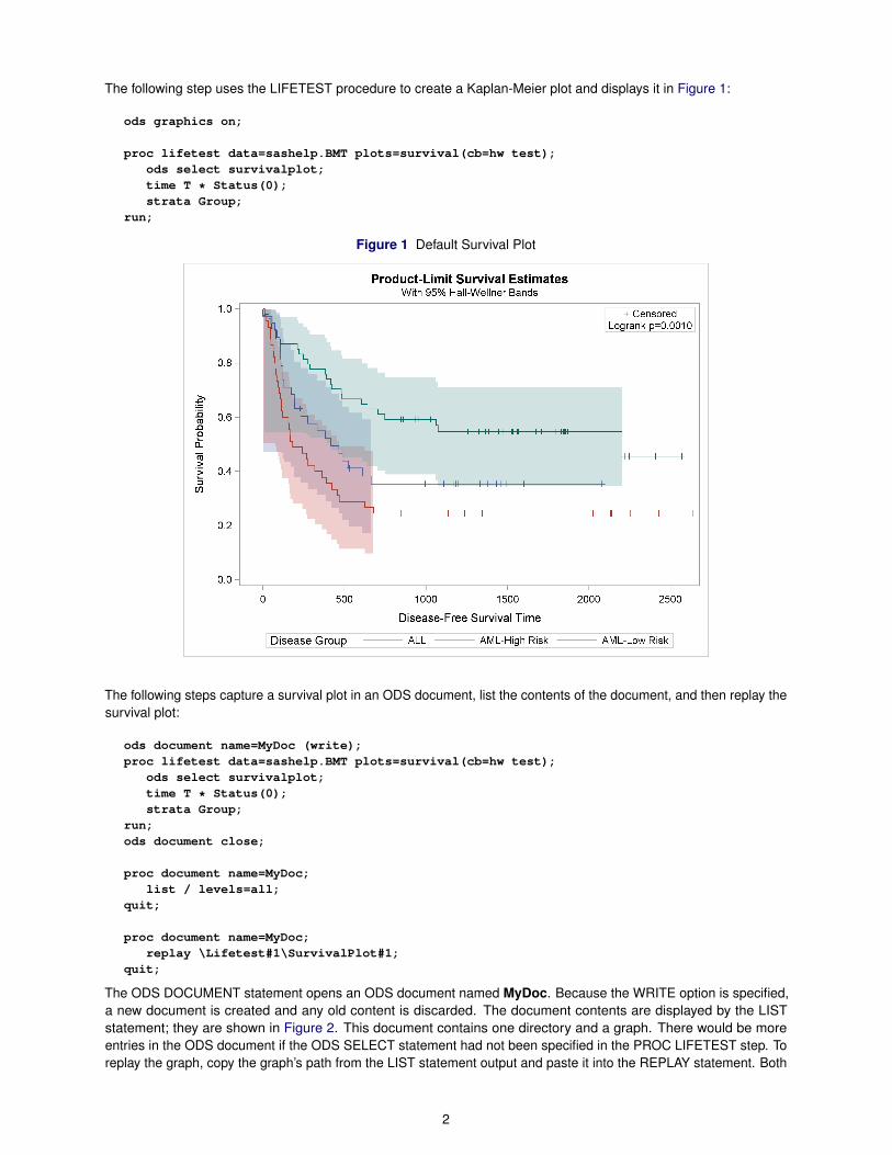
The following step uses the LIFETEST procedure to create a Kaplan-Meier plot and displays it in Figure 1:

ods graphics on;

proc lifetest data=sashelp.BMT plots=survival(cb=hw test);ods select survivalplot;time T * Status(0);strata Group;

run;

Figure 1 Default Survival Plot

The following steps capture a survival plot in an ODS document, list the contents of the document, and then replay thesurvival plot:

ods document name=MyDoc (write);proc lifetest data=sashelp.BMT plots=survival(cb=hw test);

ods select survivalplot;time T * Status(0);strata Group;

run;ods document close;

proc document name=MyDoc;list / levels=all;

quit;

proc document name=MyDoc;replay \Lifetest#1\SurvivalPlot#1;

quit;

The ODS DOCUMENT statement opens an ODS document named MyDoc. Because the WRITE option is specified,a new document is created and any old content is discarded. The document contents are displayed by the LISTstatement; they are shown in Figure 2. This document contains one directory and a graph. There would be moreentries in the ODS document if the ODS SELECT statement had not been specified in the PROC LIFETEST step. Toreplay the graph, copy the graph’s path from the LIST statement output and paste it into the REPLAY statement. Both

2

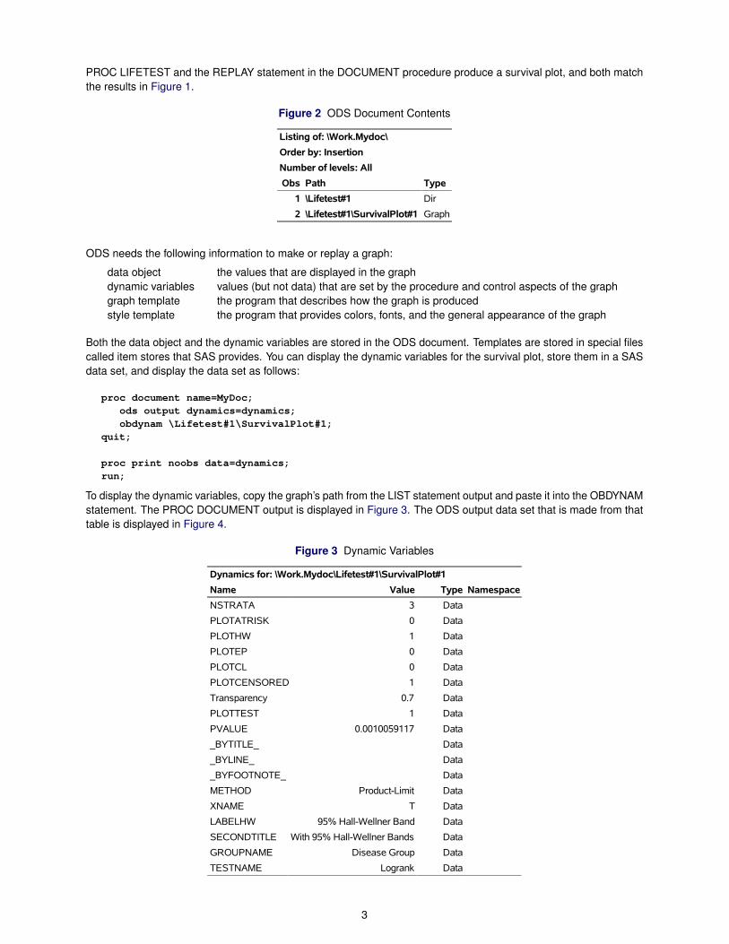
PROC LIFETEST and the REPLAY statement in the DOCUMENT procedure produce a survival plot, and both matchthe results in Figure 1.

Figure 2 ODS Document Contents

Listing of: \Work.Mydoc\

Order by: Insertion

Number of levels: All

Obs Path Type

1 \Lifetest#1 Dir

2 \Lifetest#1\SurvivalPlot#1 Graph

ODS needs the following information to make or replay a graph:

data object the values that are displayed in the graphdynamic variables values (but not data) that are set by the procedure and control aspects of the graphgraph template the program that describes how the graph is producedstyle template the program that provides colors, fonts, and the general appearance of the graph

Both the data object and the dynamic variables are stored in the ODS document. Templates are stored in special filescalled item stores that SAS provides. You can display the dynamic variables for the survival plot, store them in a SASdata set, and display the data set as follows:

proc document name=MyDoc;ods output dynamics=dynamics;obdynam \Lifetest#1\SurvivalPlot#1;

quit;

proc print noobs data=dynamics;run;

To display the dynamic variables, copy the graph’s path from the LIST statement output and paste it into the OBDYNAMstatement. The PROC DOCUMENT output is displayed in Figure 3. The ODS output data set that is made from thattable is displayed in Figure 4.

Figure 3 Dynamic Variables

Dynamics for: \Work.Mydoc\Lifetest#1\SurvivalPlot#1

Name Value Type Namespace

NSTRATA 3 Data

PLOTATRISK 0 Data

PLOTHW 1 Data

PLOTEP 0 Data

PLOTCL 0 Data

PLOTCENSORED 1 Data

Transparency 0.7 Data

PLOTTEST 1 Data

PVALUE 0.0010059117 Data

_BYTITLE_ Data

_BYLINE_ Data

_BYFOOTNOTE_ Data

METHOD Product-Limit Data

XNAME T Data

LABELHW 95% Hall-Wellner Band Data

SECONDTITLE With 95% Hall-Wellner Bands Data

GROUPNAME Disease Group Data

TESTNAME Logrank Data

3

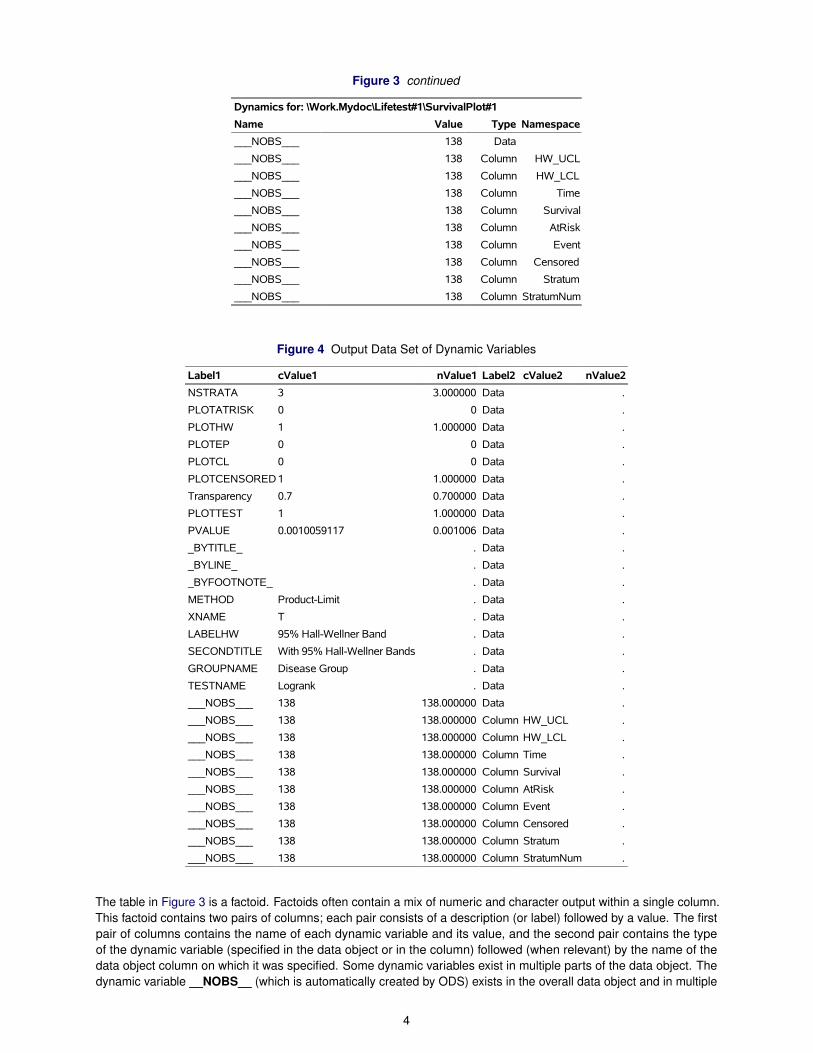
Figure 3 continued

Dynamics for: \Work.Mydoc\Lifetest#1\SurvivalPlot#1

Name Value Type Namespace

___NOBS___ 138 Data

___NOBS___ 138 Column HW_UCL

___NOBS___ 138 Column HW_LCL

___NOBS___ 138 Column Time

___NOBS___ 138 Column Survival

___NOBS___ 138 Column AtRisk

___NOBS___ 138 Column Event

___NOBS___ 138 Column Censored

___NOBS___ 138 Column Stratum

___NOBS___ 138 Column StratumNum

Figure 4 Output Data Set of Dynamic Variables

Label1 cValue1 nValue1 Label2 cValue2 nValue2

NSTRATA 3 3.000000 Data .

PLOTATRISK 0 0 Data .

PLOTHW 1 1.000000 Data .

PLOTEP 0 0 Data .

PLOTCL 0 0 Data .

PLOTCENSORED 1 1.000000 Data .

Transparency 0.7 0.700000 Data .

PLOTTEST 1 1.000000 Data .

PVALUE 0.0010059117 0.001006 Data .

_BYTITLE_ . Data .

_BYLINE_ . Data .

_BYFOOTNOTE_ . Data .

METHOD Product-Limit . Data .

XNAME T . Data .

LABELHW 95% Hall-Wellner Band . Data .

SECONDTITLE With 95% Hall-Wellner Bands . Data .

GROUPNAME Disease Group . Data .

TESTNAME Logrank . Data .

___NOBS___ 138 138.000000 Data .

___NOBS___ 138 138.000000 Column HW_UCL .

___NOBS___ 138 138.000000 Column HW_LCL .

___NOBS___ 138 138.000000 Column Time .

___NOBS___ 138 138.000000 Column Survival .

___NOBS___ 138 138.000000 Column AtRisk .

___NOBS___ 138 138.000000 Column Event .

___NOBS___ 138 138.000000 Column Censored .

___NOBS___ 138 138.000000 Column Stratum .

___NOBS___ 138 138.000000 Column StratumNum .

The table in Figure 3 is a factoid. Factoids often contain a mix of numeric and character output within a single column.This factoid contains two pairs of columns; each pair consists of a description (or label) followed by a value. The firstpair of columns contains the name of each dynamic variable and its value, and the second pair contains the typeof the dynamic variable (specified in the data object or in the column) followed (when relevant) by the name of thedata object column on which it was specified. Some dynamic variables exist in multiple parts of the data object. Thedynamic variable __NOBS__ (which is automatically created by ODS) exists in the overall data object and in multiple

4

columns. Figure 3 shows that not all dynamic variables have been set to values. This is both common and reasonable.

The Name column in Figure 3 becomes the Label1 variable in the output data set displayed in Figure 4. The Valuecolumn in Figure 3 becomes two output data set variables, cValue1 and nValue1. Similarly, the Type column becomesLabel2, and the Namespace column becomes cValue2 and nValue2. The variables nValue1 and nValue2 arenumeric, and the variables cValue1 and cValue2 are character. Numeric values are captured in two forms: the actualnumeric values are captured in the nValuen numeric variables, and formatted numeric values are captured in thecValuen character variables. Character values are captured in the cValuen variables; the nValuen variables havemissing values for character variables.

You can replay the graph and explicitly specify that the values of the dynamic variables come from a data set (ratherthan from the dynamic variables that are stored in the ODS document):

proc document name=MyDoc;replay \Lifetest#1\SurvivalPlot#1 / dynamdata=dynamics;

quit;

The REPLAY statement replays the graph. The DYNAMDATA= option names the data set that contains the dynamicvariables. The results again match those in Figure 1.

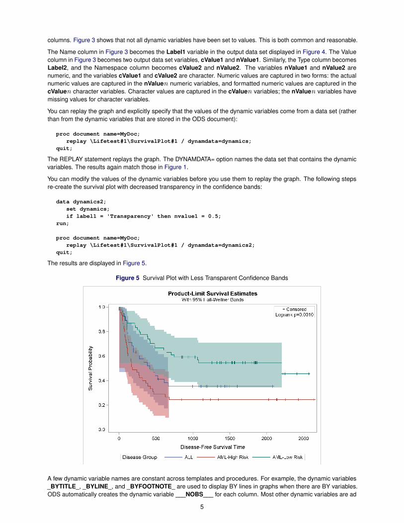
You can modify the values of the dynamic variables before you use them to replay the graph. The following stepsre-create the survival plot with decreased transparency in the confidence bands:

data dynamics2;set dynamics;if label1 = 'Transparency' then nvalue1 = 0.5;

run;

proc document name=MyDoc;replay \Lifetest#1\SurvivalPlot#1 / dynamdata=dynamics2;

quit;

The results are displayed in Figure 5.

Figure 5 Survival Plot with Less Transparent Confidence Bands

A few dynamic variable names are constant across templates and procedures. For example, the dynamic variables_BYTITLE_, _BYLINE_, and _BYFOOTNOTE_ are used to display BY lines in graphs when there are BY variables.ODS automatically creates the dynamic variable ___NOBS___ for each column. Most other dynamic variables are ad

5

hoc, although you might see patterns within procedures or graph types. You might need to look at the graph templateand the GTL documentation to better understand the purpose of some dynamic variables.

You can modify both the graph template and the dynamic variables. Several parts of this paper use the method oftemplate modification for the survival plot that is discussed in detail in Chapter 23, “Customizing the Kaplan-MeierSurvival Plot” (SAS/STAT User’s Guide). That method is used but not explained in this paper. The rest of the paperassumes that you have run the following steps to include the macros and macro variables:

data _null_;%let url = //support.sas.com/documentation/onlinedoc/stat/ex_code/141;infile "http:&url/templft.html" device=url;

file 'macros.tmp';retain pre 0;input;if index(_infile_, '</pre>') then pre = 0;if pre then put _infile_;if index(_infile_, '<pre>') then pre = 1;

run;

%inc 'macros.tmp' / nosource;

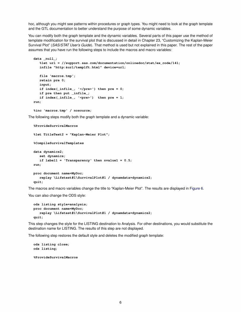
The following steps modify both the graph template and a dynamic variable:

%ProvideSurvivalMacros

%let TitleText2 = "Kaplan-Meier Plot";

%CompileSurvivalTemplates

data dynamics2;set dynamics;if label1 = 'Transparency' then nvalue1 = 0.5;

run;

proc document name=MyDoc;replay \Lifetest#1\SurvivalPlot#1 / dynamdata=dynamics2;

quit;

The macros and macro variables change the title to “Kaplan-Meier Plot”. The results are displayed in Figure 6.

You can also change the ODS style:

ods listing style=analysis;proc document name=MyDoc;

replay \Lifetest#1\SurvivalPlot#1 / dynamdata=dynamics2;quit;

This step changes the style for the LISTING destination to Analysis. For other destinations, you would substitute thedestination name for LISTING. The results of this step are not displayed.

The following step restores the default style and deletes the modified graph template:

ods listing close;ods listing;

%ProvideSurvivalMacros

6

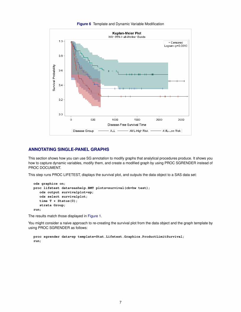
Figure 6 Template and Dynamic Variable Modification

ANNOTATING SINGLE-PANEL GRAPHS

This section shows how you can use SG annotation to modify graphs that analytical procedures produce. It shows youhow to capture dynamic variables, modify them, and create a modified graph by using PROC SGRENDER instead ofPROC DOCUMENT.

This step runs PROC LIFETEST, displays the survival plot, and outputs the data object to a SAS data set:

ods graphics on;proc lifetest data=sashelp.BMT plots=survival(cb=hw test);

ods output survivalplot=sp;ods select survivalplot;time T * Status(0);strata Group;

run;

The results match those displayed in Figure 1.

You might consider a naive approach to re-creating the survival plot from the data object and the graph template byusing PROC SGRENDER as follows:

proc sgrender data=sp template=Stat.Lifetest.Graphics.ProductLimitSurvival;run;

7

Figure 7 Dynamic Information Missing

For some graphs, this might completely work (if there are no dynamic variables) or it might completely fail (for example,if there is one graph statement and a critical part depends on dynamic variables). The preceding step partially works.The results are displayed in Figure 7. In this example, the inset box in the top right portion of the graph, part of thetitle, and the confidence bands are all missing because all of them depend on dynamic variables.

You can run the following step to create the graph, output the data object to a SAS data set, and capture the dynamicvariables in an ODS document:

ods document name=MyDoc (write);proc lifetest data=sashelp.BMT plots=survival(cb=hw test);

ods output survivalplot=sp;ods select survivalplot;time T * Status(0);strata Group;

run;ods document close;

You can list the contents of the ODS document as follows:

proc document name=MyDoc;list / levels=all;

quit;

You can store the names of the dynamic variables and their values in a SAS data set as follows:

proc document name=MyDoc;ods output dynamics=outdynam;obdynam \Lifetest#1\SurvivalPlot#1;

quit;

To display the dynamic variables, copy the graph’s path from the LIST statement output and paste it into the OBDYNAMstatement.

The SG annotation data set Anno (displayed in Figure 8) is used to add a date to the top right corner of the graph anda watermark diagonally across the graph (as shown in Figure 9):

8

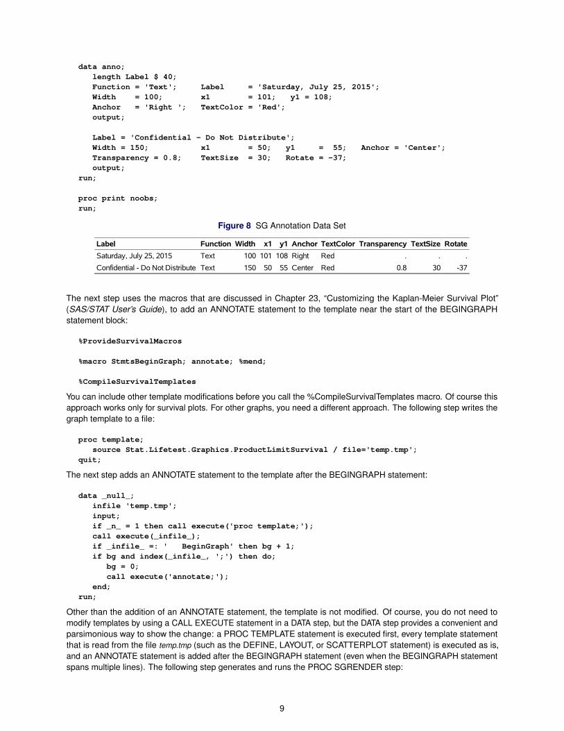
data anno;length Label $ 40;Function = 'Text'; Label = 'Saturday, July 25, 2015';Width = 100; x1 = 101; y1 = 108;Anchor = 'Right '; TextColor = 'Red';output;

Label = 'Confidential - Do Not Distribute';Width = 150; x1 = 50; y1 = 55; Anchor = 'Center';Transparency = 0.8; TextSize = 30; Rotate = -37;output;

run;

proc print noobs;run;

Figure 8 SG Annotation Data Set

Label Function Width x1 y1 Anchor TextColor Transparency TextSize Rotate

Saturday, July 25, 2015 Text 100 101 108 Right Red . . .

Confidential - Do Not Distribute Text 150 50 55 Center Red 0.8 30 -37

The next step uses the macros that are discussed in Chapter 23, “Customizing the Kaplan-Meier Survival Plot”(SAS/STAT User’s Guide), to add an ANNOTATE statement to the template near the start of the BEGINGRAPHstatement block:

%ProvideSurvivalMacros

%macro StmtsBeginGraph; annotate; %mend;

%CompileSurvivalTemplates

You can include other template modifications before you call the %CompileSurvivalTemplates macro. Of course thisapproach works only for survival plots. For other graphs, you need a different approach. The following step writes thegraph template to a file:

proc template;source Stat.Lifetest.Graphics.ProductLimitSurvival / file='temp.tmp';

quit;

The next step adds an ANNOTATE statement to the template after the BEGINGRAPH statement:

data _null_;infile 'temp.tmp';input;if _n_ = 1 then call execute('proc template;');call execute(_infile_);if _infile_ =: ' BeginGraph' then bg + 1;if bg and index(_infile_, ';') then do;

bg = 0;call execute('annotate;');

end;run;

Other than the addition of an ANNOTATE statement, the template is not modified. Of course, you do not need tomodify templates by using a CALL EXECUTE statement in a DATA step, but the DATA step provides a convenient andparsimonious way to show the change: a PROC TEMPLATE statement is executed first, every template statementthat is read from the file temp.tmp (such as the DEFINE, LAYOUT, or SCATTERPLOT statement) is executed as is,and an ANNOTATE statement is added after the BEGINGRAPH statement (even when the BEGINGRAPH statementspans multiple lines). The following step generates and runs the PROC SGRENDER step:

9

data _null_;set outdynam(where=(label1 ne '___NOBS___')) end=eof;if nmiss(nvalue1) and cvalue1 = '.' then cvalue1 = ' ';if _n_ = 1 then do;

call execute('proc sgrender data=sp sganno=anno');call execute('template=Stat.Lifetest.Graphics.ProductLimitSurvival;');call execute('dynamic');

end;if label1 = 'Transparency' then cvalue1 = '0.9';if cvalue1 ne ' ' then

call execute(catx(' ', label1, '=',ifc(n(nvalue1), cvalue1, quote(trim(cvalue1)))));

if eof then call execute('; run;');run;

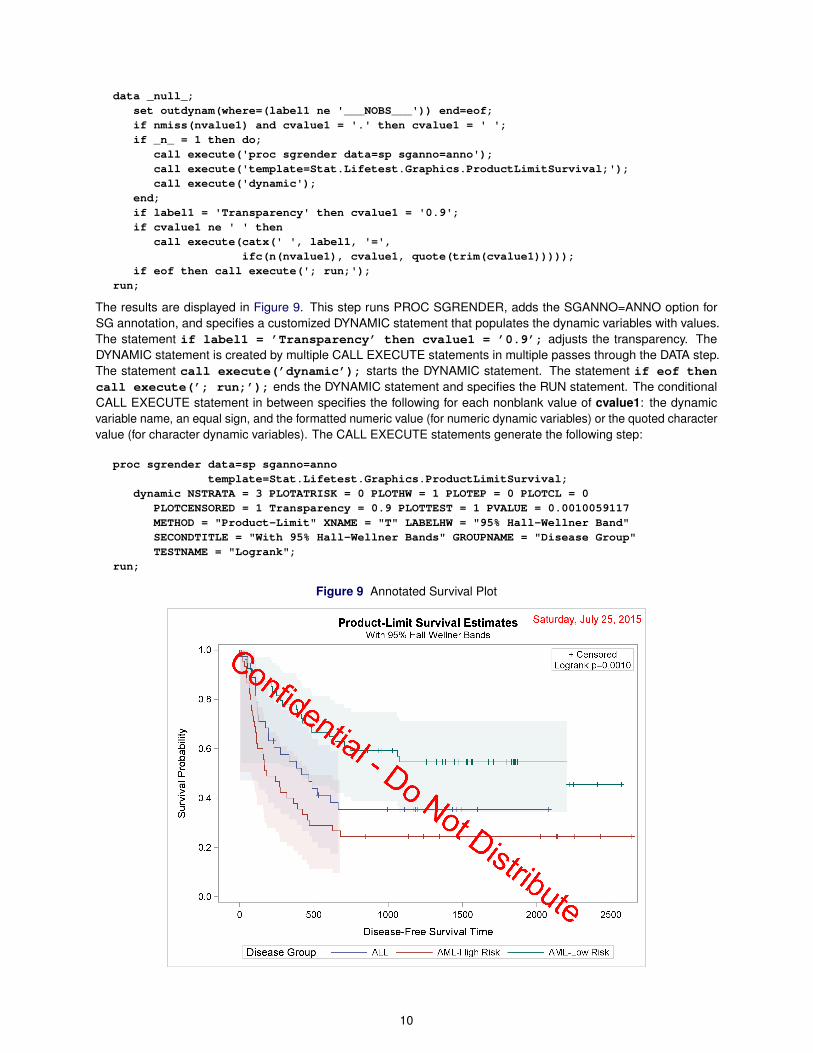
The results are displayed in Figure 9. This step runs PROC SGRENDER, adds the SGANNO=ANNO option forSG annotation, and specifies a customized DYNAMIC statement that populates the dynamic variables with values.The statement if label1 = ’Transparency’ then cvalue1 = ’0.9’; adjusts the transparency. TheDYNAMIC statement is created by multiple CALL EXECUTE statements in multiple passes through the DATA step.The statement call execute(’dynamic’); starts the DYNAMIC statement. The statement if eof thencall execute(’; run;’); ends the DYNAMIC statement and specifies the RUN statement. The conditionalCALL EXECUTE statement in between specifies the following for each nonblank value of cvalue1: the dynamicvariable name, an equal sign, and the formatted numeric value (for numeric dynamic variables) or the quoted charactervalue (for character dynamic variables). The CALL EXECUTE statements generate the following step:

proc sgrender data=sp sganno=annotemplate=Stat.Lifetest.Graphics.ProductLimitSurvival;

dynamic NSTRATA = 3 PLOTATRISK = 0 PLOTHW = 1 PLOTEP = 0 PLOTCL = 0PLOTCENSORED = 1 Transparency = 0.9 PLOTTEST = 1 PVALUE = 0.0010059117METHOD = "Product-Limit" XNAME = "T" LABELHW = "95% Hall-Wellner Band"SECONDTITLE = "With 95% Hall-Wellner Bands" GROUPNAME = "Disease Group"TESTNAME = "Logrank";

run;

Figure 9 Annotated Survival Plot

10

The following step deletes the modified template:

proc template;delete Stat.Lifetest.Graphics.ProductLimitSurvival;

quit;

Assuming that you are creating exactly one graph and then annotating it, you can use the %ProcAnno macro in thefollowing steps to process the template and the dynamic variables:

%macro procanno(data=, template=, anno=anno, document=mydoc);proc document name=&document;

ods exclude properties;ods output properties=__p(where=(type='Graph'));list / levels=all;

quit;

data _null_;set __p;call execute("proc document name=&document;");call execute("ods exclude dynamics;");call execute("ods output dynamics=__outdynam;");call execute(catx(' ', "obdynam", path, ';'));

run;

proc template;source &template / file='temp.tmp';

quit;

data _null_;infile 'temp.tmp';input;if _n_ = 1 then call execute('proc template;');call execute(_infile_);if _infile_ =: ' BeginGraph' then bg + 1;if bg and index(_infile_, ';') then do;

bg = 0;call execute('annotate;');

end;run;

data _null_;set __outdynam(where=(label1 ne '___NOBS___')) end=eof;if nmiss(nvalue1) and cvalue1 = '.' then cvalue1 = ' ';if _n_ = 1 then do;

call execute("proc sgrender data=&data sganno=&anno");call execute("template=&template;");call execute('dynamic');

end;if cvalue1 ne ' ' then

call execute(catx(' ', label1, '=',ifc(n(nvalue1), cvalue1, quote(trim(cvalue1)))));

if eof then call execute('; run;');run;

proc template;delete &template;

quit;%mend;

%procanno(data=sp, template=Stat.Lifetest.Graphics.ProductLimitSurvival)

The preceding step illustrates the general way to modify graph templates and does not require the techniquesdescribed in Chapter 23, “Customizing the Kaplan-Meier Survival Plot” (SAS/STAT User’s Guide). You create thegraph, capture the dynamic variables in an ODS document, and create the SG annotation data set; the macro does

11

the rest. The results are not displayed here. If you want to modify the graph template, you can do that before youcall the macro. You could instead enhance the %ProcAnno macro to accept template modification statements. Themodifications would be inserted in the DATA step that processes the file temp.tmp. The next section illustrates.

ANNOTATING MULTIPLE-PANEL GRAPHS

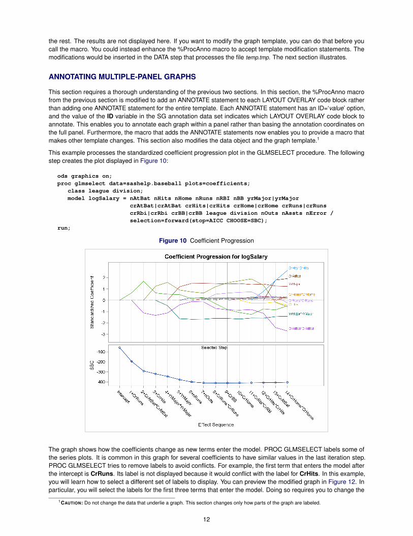
This section requires a thorough understanding of the previous two sections. In this section, the %ProcAnno macrofrom the previous section is modified to add an ANNOTATE statement to each LAYOUT OVERLAY code block ratherthan adding one ANNOTATE statement for the entire template. Each ANNOTATE statement has an ID=‘value’ option,and the value of the ID variable in the SG annotation data set indicates which LAYOUT OVERLAY code block toannotate. This enables you to annotate each graph within a panel rather than basing the annotation coordinates onthe full panel. Furthermore, the macro that adds the ANNOTATE statements now enables you to provide a macro thatmakes other template changes. This section also modifies the data object and the graph template.1

This example processes the standardized coefficient progression plot in the GLMSELECT procedure. The followingstep creates the plot displayed in Figure 10:

ods graphics on;proc glmselect data=sashelp.baseball plots=coefficients;

class league division;model logSalary = nAtBat nHits nHome nRuns nRBI nBB yrMajor|yrMajor

crAtBat|crAtBat crHits|crHits crHome|crHome crRuns|crRunscrRbi|crRbi crBB|crBB league division nOuts nAssts nError /selection=forward(stop=AICC CHOOSE=SBC);

run;

Figure 10 Coefficient Progression

The graph shows how the coefficients change as new terms enter the model. PROC GLMSELECT labels some ofthe series plots. It is common in this graph for several coefficients to have similar values in the last iteration step.PROC GLMSELECT tries to remove labels to avoid conflicts. For example, the first term that enters the model afterthe intercept is CrRuns. Its label is not displayed because it would conflict with the label for CrHits. In this example,you will learn how to select a different set of labels to display. You can preview the modified graph in Figure 12. Inparticular, you will select the labels for the first three terms that enter the model. Doing so requires you to change the

1CAUTION: Do not change the data that underlie a graph. This section changes only how parts of the graph are labeled.

12

data object. Then you can add annotation to highlight the selected model. In PROC GLMSELECT, the final modeldoes not usually correspond to the end of the progression of the coefficients. In this case, the final model correspondsto the vertical reference line at step 9 in the graph, which is labeled as “9+CrBB” on the X axis and indicates that thevariable CrBB entered the model at step 9.

You begin by creating a data object and storing the graph along with the dynamic variables in an ODS document:

ods document name=MyDoc (write);proc glmselect data=sashelp.baseball plots=coefficients;

ods select CoefficientPanel;ods output CoefficientPanel=cp;class league division;model logSalary = nAtBat nHits nHome nRuns nRBI nBB yrMajor|yrMajor

crAtBat|crAtBat crHits|crHits crHome|crHome crRuns|crRunscrRbi|crRbi crBB|crBB league division nOuts nAssts nError /selection=forward(stop=AICC CHOOSE=SBC);

run;ods document close;

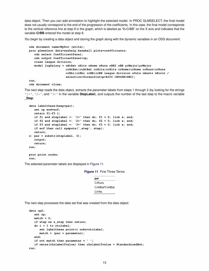
The next step reads the data object, extracts the parameter labels from steps 1 through 3 (by looking for the strings'1+', '2+', and '3+' in the variable StepLabel), and outputs the number of the last step to the macro variable_Step:

data labelthese(keep=par);set cp end=eof;retain f1-f3 1;if f1 and steplabel =: '1+' then do; f1 = 0; link s; end;if f2 and steplabel =: '2+' then do; f2 = 0; link s; end;if f3 and steplabel =: '3+' then do; f3 = 0; link s; end;if eof then call symputx('_step', step);return;

s: par = substr(steplabel, 3);output;return;

run;

proc print noobs;run;

The selected parameter labels are displayed in Figure 11.

Figure 11 First Three Terms

par

CrRuns

CrAtBat*CrAtBat

CrHits

The next step processes the data set that was created from the data object:

data cp2;set cp;match = 0;if step ne &_step then return;do i = 1 to ntolabel;

set labelthese point=i nobs=ntolabel;match + (par = parameter);

end;if not match then parameter = ' ';if nmiss(rhslabelYvalue) then rhslabelYvalue = StandardizedEst;

run;

13

The last part of the data set contains the coordinates and strings that are needed to label each profile. The DATAstep sets the parameter value to blank in the last step that PROC GLMSELECT considers (when the Step variablematches the _Step macro variable, which corresponds to the end of the profiles in the graph) for all but the first threeterms (that is, for all but those that match the labels stored in the data set Label). When the Y coordinate for a label ismissing (because PROC GLMSELECT suppressed it as a result of collisions), the Y coordinate value is restored.

The next step creates the %Tweak macro, which contains the code that modifies the graph template:

%macro tweak;if index(_infile_, 'datalabel=PARAMETER') then

_infile_ = tranwrd(_infile_, 'datalabel','markercharacterposition=right markercharacter');

if index(_infile_, 'curvelabel="Selected Step"') then_infile_ = tranwrd(_infile_, 'curvelabel="Selected Step"', ' ');

%mend;

The macro uses two IF statements, each of which makes a change:

� The first IF statement removes the DATALABEL= option in a SCATTERPLOT statement and instead specifies theMARKERCHARACTER= option. You can use the MARKERCHARACTER= option to position labels precisely ata point. In contrast, the DATALABEL= option moves labels that conflict. The first IF statement also adds theMARKERCHARACTERPOSITION=RIGHT option so that labels are positioned to the right of the coordinates.The TRANWRD (translate word) function makes the change, substituting a longer string for a shorter string.

� The second IF statement removes the “Selected Step” label for the reference line in the bottom panel. You willadd it back in through SG annotation.

The next step creates the SG annotation data set:

data anno;length ID $ 3 Function $ 9 Label $ 40;retain x1Space y1Space x2Space y2Space 'DataPercent' Direction 'In';length Anchor $ 10 xC1 xC2 $ 20;retain Scale 1e-12 Width 100 WidthUnit 'Data' CornerRadius 0.8

TextSize 7 TextWeight 'Bold'LineThickness 1.2 DiscreteOffset -0.3 LineColor 'Green';

ID = 'LO1'; Function = 'Text';Anchor = 'Right'; TextColor = 'Green';x1 = 55; y1 = 94;Label = 'Coefficients for the Selected Model'; output;

Function = 'Line'; x1 = .;x1Space = 'DataValue'; x2Space = x1Space;xc1 = '9+CrBB'; xc2 = '8+CrRuns*CrRuns';y1 = 94; y2 = 94; output;

Function = 'Rectangle'; y1Space = 'WallPercent';Anchor = 'BottomLeft'; y1 = 10;Height = 80; Width = 0.6; output;

ID = 'LO3'; Width = 100;Function = 'Text '; Label = 'Selected Value';x1Space = 'DataPercent'; y1Space = x1Space;Anchor = 'Left'; TextColor = 'Blue';x1 = 86; y1 = 84; output;

Function = 'Arrow'; LineColor = 'Blue';x1Space = 'DataValue'; x2Space = x1Space;xc1 = '9+CrBB'; xc2 = '12+CrHits*CrHits';y1 = 4; y2 = 83;DiscreteOffset = .1; x1 = .; output;

run;

14

The SG annotation data set has five observations (the effects of which are shown in Figure 12):1. the text string ‘Coefficients for the Selected Model’ (ID = 'LO1')2. a line from the text string to the rectangle (ID = 'LO1')3. a rectangle that has rounded corners and surrounds the coefficients for the selected model (ID = 'LO1')4. the text string ‘Selected Value’ (ID = 'LO3')5. an arrow that points from the text string to the selected value (ID = 'LO3')

The new, advanced template processing macro, %ProcAnnoAdv (enhanced from %ProcAnno), is next:

%macro procannoadv(data=, template=, anno=anno, document=mydoc, adjust=,overallanno=1);

proc document name=&document;ods exclude properties;ods output properties=__p(where=(type='Graph'));list / levels=all;

quit;

data _null_;set __p;call execute("proc document name=&document;");call execute("ods exclude dynamics;");call execute("ods output dynamics=__outdynam;");call execute(catx(' ', "obdynam", path, ';'));

run;

proc template;source &template / file='temp.tmp';

quit;

data _null_;infile 'temp.tmp';input;if _n_ = 1 then call execute('proc template;');%if &adjust ne %then %do; %&adjust %end;call execute(_infile_);if &overallanno and _infile_ =: ' BeginGraph' then bg + 1;else if not &overallanno and index(_infile_, ' layout overlay')

then lo + 1;if bg and index(_infile_, ';') then do;

bg = 0;call execute('annotate;');

end;if lo and index(_infile_, ';') then do;

lo = 0;lonum + 1;call execute(catt('annotate / id="LO', lonum, '";'));

end;run;

data _null_;set __outdynam(where=(label1 ne '___NOBS___')) end=eof;if nmiss(nvalue1) and cvalue1 = '.' then cvalue1 = ' ';if _n_ = 1 then do;

call execute("proc sgrender data=&data");if symget('anno') ne ' ' then call execute("sganno=&anno");call execute("template=&template;");call execute('dynamic');

end;if cvalue1 ne ' ' then

call execute(catx(' ', label1, '=',ifc(n(nvalue1), cvalue1, quote(trim(cvalue1)))));

if eof then call execute('; run;');run;

15

proc template;delete &template;

quit;%mend;

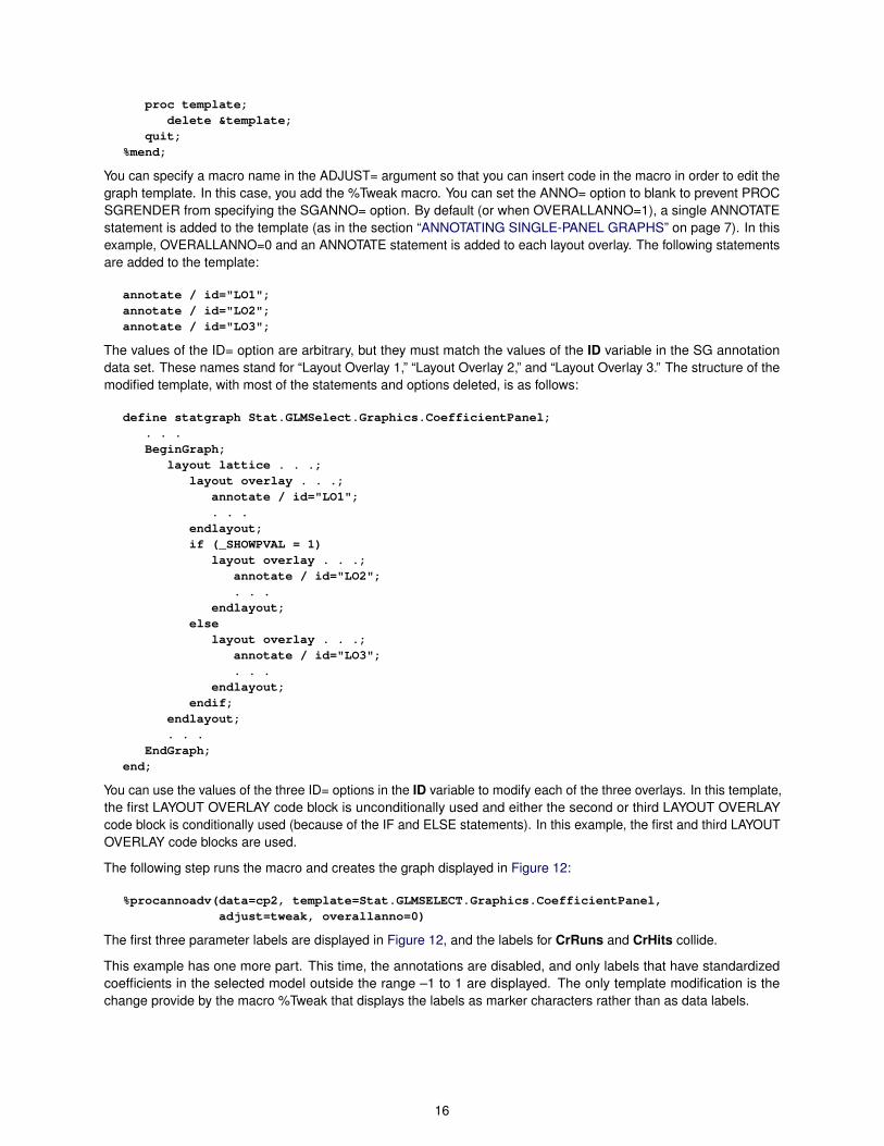
You can specify a macro name in the ADJUST= argument so that you can insert code in the macro in order to edit thegraph template. In this case, you add the %Tweak macro. You can set the ANNO= option to blank to prevent PROCSGRENDER from specifying the SGANNO= option. By default (or when OVERALLANNO=1), a single ANNOTATEstatement is added to the template (as in the section “ANNOTATING SINGLE-PANEL GRAPHS” on page 7). In thisexample, OVERALLANNO=0 and an ANNOTATE statement is added to each layout overlay. The following statementsare added to the template:

annotate / id="LO1";annotate / id="LO2";annotate / id="LO3";

The values of the ID= option are arbitrary, but they must match the values of the ID variable in the SG annotationdata set. These names stand for “Layout Overlay 1,” “Layout Overlay 2,” and “Layout Overlay 3.” The structure of themodified template, with most of the statements and options deleted, is as follows:

define statgraph Stat.GLMSelect.Graphics.CoefficientPanel;. . .BeginGraph;

layout lattice . . .;layout overlay . . .;

annotate / id="LO1";. . .

endlayout;if (_SHOWPVAL = 1)

layout overlay . . .;annotate / id="LO2";. . .

endlayout;else

layout overlay . . .;annotate / id="LO3";. . .

endlayout;endif;

endlayout;. . .

EndGraph;end;

You can use the values of the three ID= options in the ID variable to modify each of the three overlays. In this template,the first LAYOUT OVERLAY code block is unconditionally used and either the second or third LAYOUT OVERLAYcode block is conditionally used (because of the IF and ELSE statements). In this example, the first and third LAYOUTOVERLAY code blocks are used.

The following step runs the macro and creates the graph displayed in Figure 12:

%procannoadv(data=cp2, template=Stat.GLMSELECT.Graphics.CoefficientPanel,adjust=tweak, overallanno=0)

The first three parameter labels are displayed in Figure 12, and the labels for CrRuns and CrHits collide.

This example has one more part. This time, the annotations are disabled, and only labels that have standardizedcoefficients in the selected model outside the range –1 to 1 are displayed. The only template modification is thechange provide by the macro %Tweak that displays the labels as marker characters rather than as data labels.

16

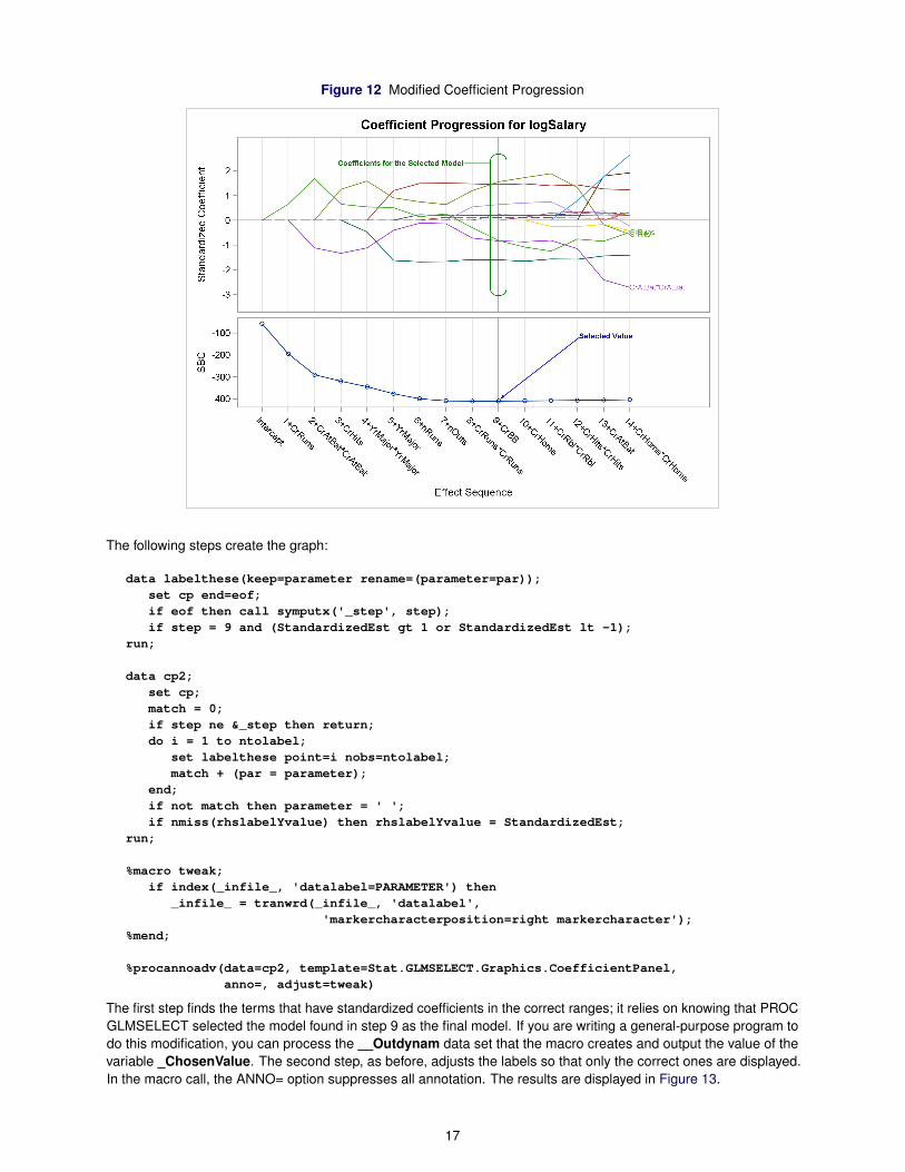
Figure 12 Modified Coefficient Progression

The following steps create the graph:

data labelthese(keep=parameter rename=(parameter=par));set cp end=eof;if eof then call symputx('_step', step);if step = 9 and (StandardizedEst gt 1 or StandardizedEst lt -1);

run;

data cp2;set cp;match = 0;if step ne &_step then return;do i = 1 to ntolabel;

set labelthese point=i nobs=ntolabel;match + (par = parameter);

end;if not match then parameter = ' ';if nmiss(rhslabelYvalue) then rhslabelYvalue = StandardizedEst;

run;

%macro tweak;if index(_infile_, 'datalabel=PARAMETER') then

_infile_ = tranwrd(_infile_, 'datalabel','markercharacterposition=right markercharacter');

%mend;

%procannoadv(data=cp2, template=Stat.GLMSELECT.Graphics.CoefficientPanel,anno=, adjust=tweak)

The first step finds the terms that have standardized coefficients in the correct ranges; it relies on knowing that PROCGLMSELECT selected the model found in step 9 as the final model. If you are writing a general-purpose program todo this modification, you can process the __Outdynam data set that the macro creates and output the value of thevariable _ChosenValue. The second step, as before, adjusts the labels so that only the correct ones are displayed.In the macro call, the ANNO= option suppresses all annotation. The results are displayed in Figure 13.

17

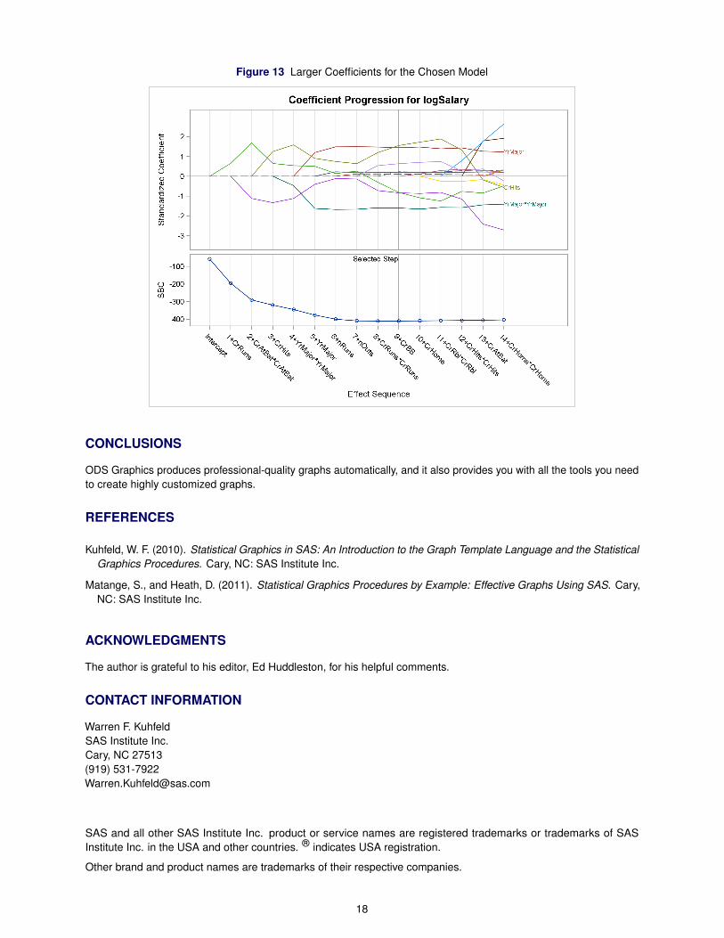
Figure 13 Larger Coefficients for the Chosen Model

CONCLUSIONS

ODS Graphics produces professional-quality graphs automatically, and it also provides you with all the tools you needto create highly customized graphs.

REFERENCES

Kuhfeld, W. F. (2010). Statistical Graphics in SAS: An Introduction to the Graph Template Language and the StatisticalGraphics Procedures. Cary, NC: SAS Institute Inc.

Matange, S., and Heath, D. (2011). Statistical Graphics Procedures by Example: Effective Graphs Using SAS. Cary,NC: SAS Institute Inc.

ACKNOWLEDGMENTS

The author is grateful to his editor, Ed Huddleston, for his helpful comments.

CONTACT INFORMATION

Warren F. KuhfeldSAS Institute Inc.Cary, NC 27513(919) 531-7922Warren.Kuhfeld@sas.com

SAS and all other SAS Institute Inc. product or service names are registered trademarks or trademarks of SASInstitute Inc. in the USA and other countries. ® indicates USA registration.

Other brand and product names are trademarks of their respective companies.

18