Antennas 2

Overview of Antennas

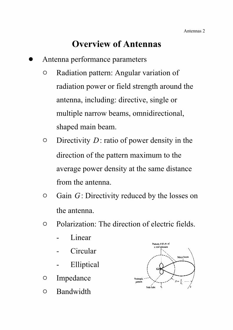
! Antenna performance parameters

" Radiation pattern: Angular variation of

radiation power or field strength around the

antenna, including: directive, single or

multiple narrow beams, omnidirectional,

shaped main beam.

" Directivity : ratio of power density in the

direction of the pattern maximum to the

average power density at the same distance

from the antenna.

" Gain : Directivity reduced by the losses on

the antenna.

" Polarization: The direction of electric fields.

- Linear

- Circular

- Elliptical

" Impedance

" Bandwidth

Antennas 3

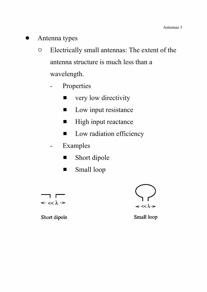
! Antenna types

" Electrically small antennas: The extent of the

antenna structure is much less than a

wavelength.

- Properties

# very low directivity

# Low input resistance

# High input reactance

# Low radiation efficiency

- Examples

# Short dipole

# Small loop

Antennas 4

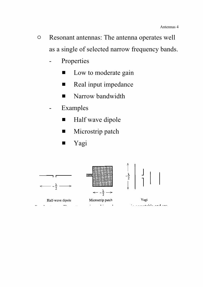
" Resonant antennas: The antenna operates well

as a single of selected narrow frequency bands.

- Properties

# Low to moderate gain

# Real input impedance

# Narrow bandwidth

- Examples

# Half wave dipole

# Microstrip patch

# Yagi

Antennas 5

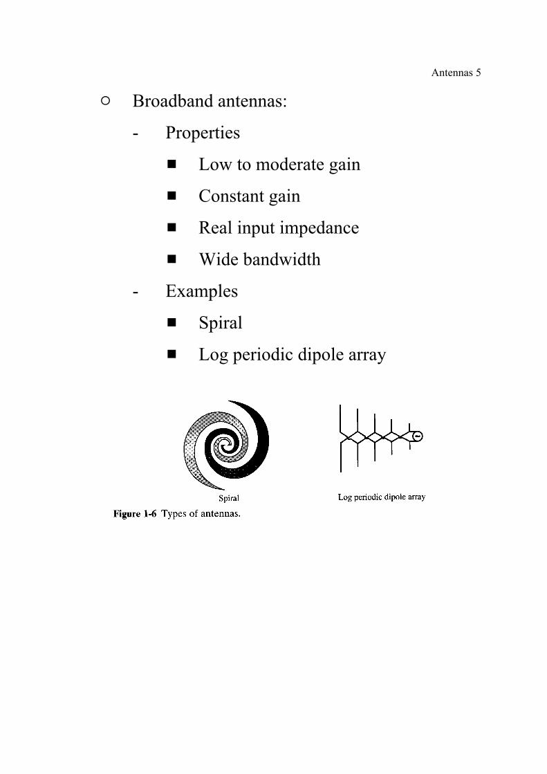
" Broadband antennas:

- Properties

# Low to moderate gain

# Constant gain

# Real input impedance

# Wide bandwidth

- Examples

# Spiral

# Log periodic dipole array

Antennas 6

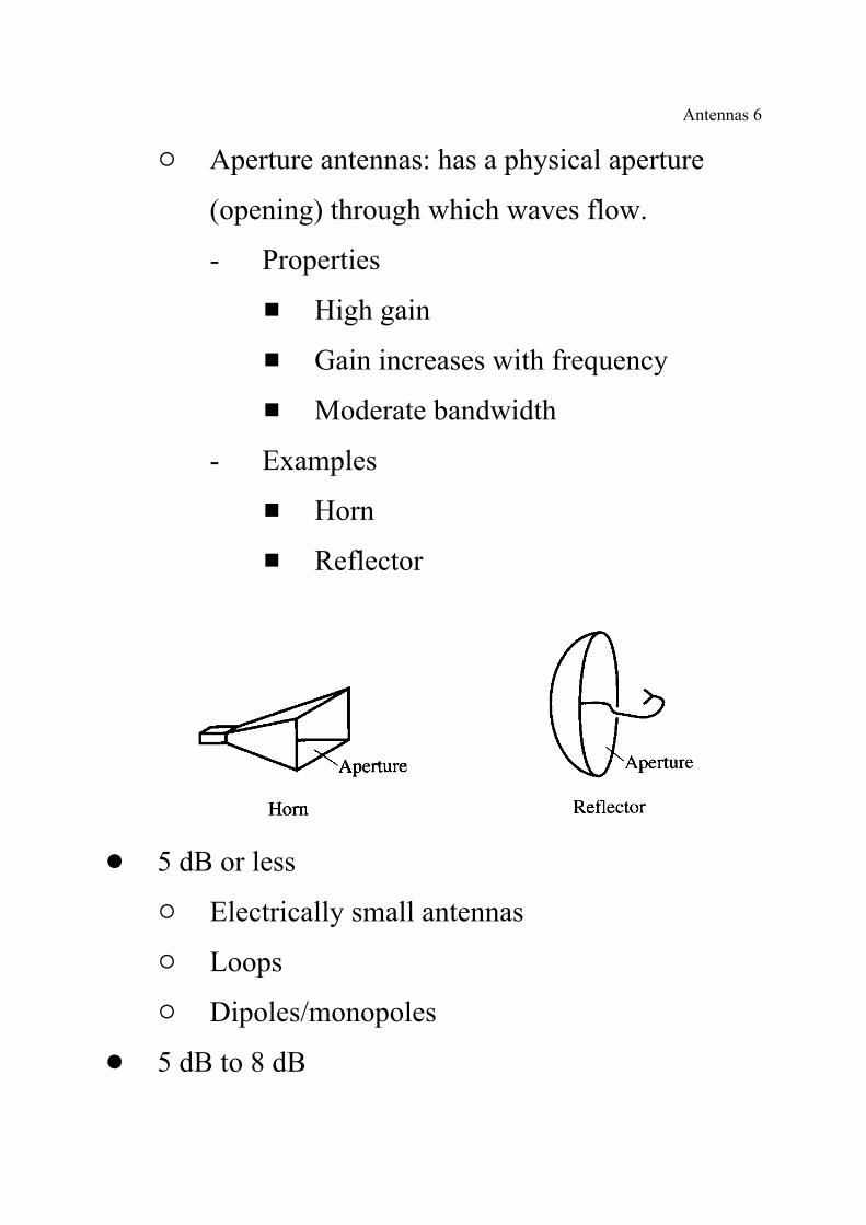
" Aperture antennas: has a physical aperture

(opening) through which waves flow.

- Properties

# High gain

# Gain increases with frequency

# Moderate bandwidth

- Examples

# Horn

# Reflector

! 5 dB or less

" Electrically small antennas

" Loops

" Dipoles/monopoles

! 5 dB to 8 dB

Antennas 7

" Microstrip Patches

" Planar frequency-independent antennas (e. g.

Spirals)

! 8 dB to 15 dB

" Yagi-Uda

" Helix (axial mode)

" Log periodic dipole array

! 15 dB and more

" Aperture antennas (Horns, Reflectors)

Antennas 8

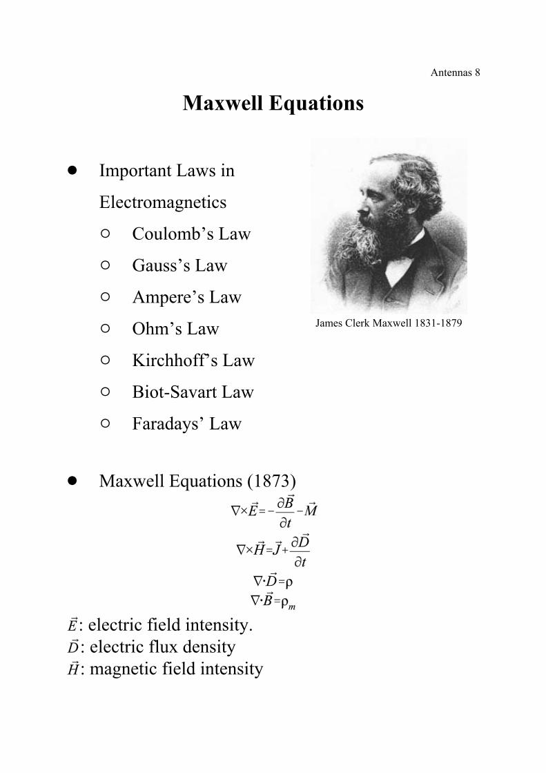
James Clerk Maxwell 1831-1879

Maxwell Equations

! Important Laws in

Electromagnetics

" Coulomb’s Law

" Gauss’s Law

" Ampere’s Law

" Ohm’s Law

" Kirchhoff’s Law

" Biot-Savart Law

" Faradays’ Law

! Maxwell Equations (1873)

: electric field intensity.: electric flux density: magnetic field intensity

Antennas 9

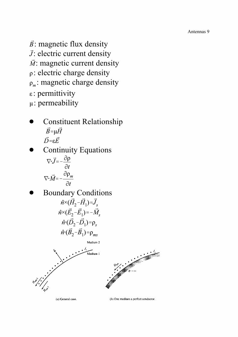
: magnetic flux density: electric current density: magnetic current density

: electric charge density: magnetic charge density

: permittivity: permeability

! Constituent Relationship

! Continuity Equations

! Boundary Conditions

Antennas 10

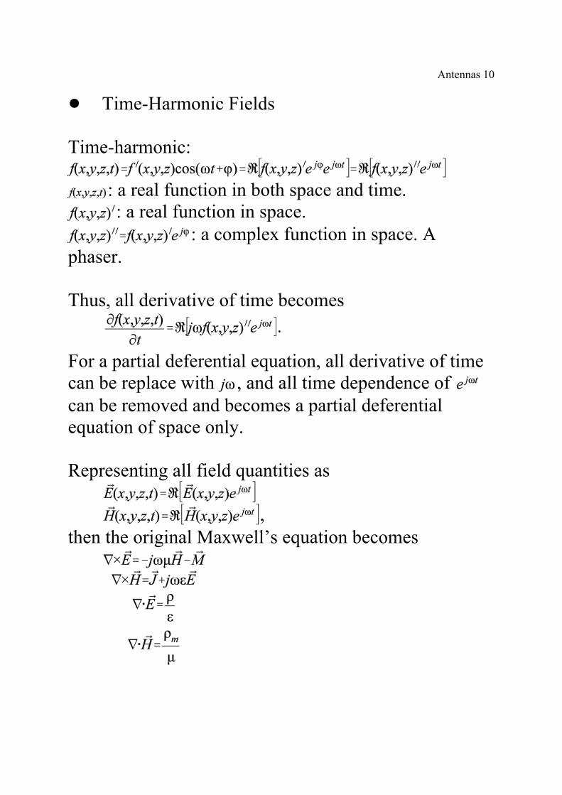
! Time-Harmonic Fields

Time-harmonic:

: a real function in both space and time.: a real function in space.

: a complex function in space. Aphaser.

Thus, all derivative of time becomes.

For a partial deferential equation, all derivative of timecan be replace with , and all time dependence of can be removed and becomes a partial deferentialequation of space only.

Representing all field quantities as

,then the original Maxwell’s equation becomes

Antennas 11

! Power Relationship

! Poynting vector:

! Solution of Maxwell’s EquationsNote all the field and source quantities are functions ofspace only. The wave equations of potentials becomes

,

where is called the wave number. The aboveequations are called nonhomogeneous Helmholtz’sequations. The Lorentz condition becomes

Also

Antennas 12

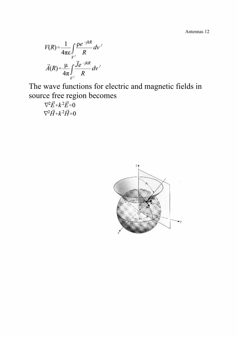
The wave functions for electric and magnetic fields insource free region becomes

Antennas 13

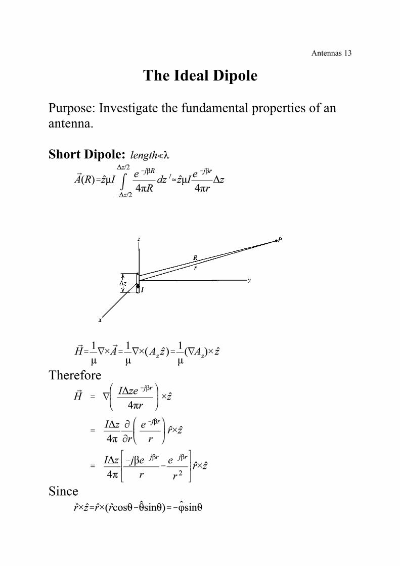
The Ideal Dipole

Purpose: Investigate the fundamental properties of anantenna.

Short Dipole:

Therefore

Since

Antennas 14

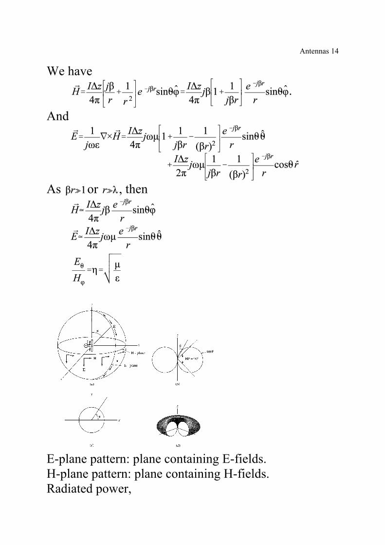
We have

.

And

As or , then

E-plane pattern: plane containing E-fields.H-plane pattern: plane containing H-fields.Radiated power,

Antennas 15

To sum up, at far field1. Spherical TEM waves.2. Wave impedance equal the intrinsic impedance

.

3. Real power flow.

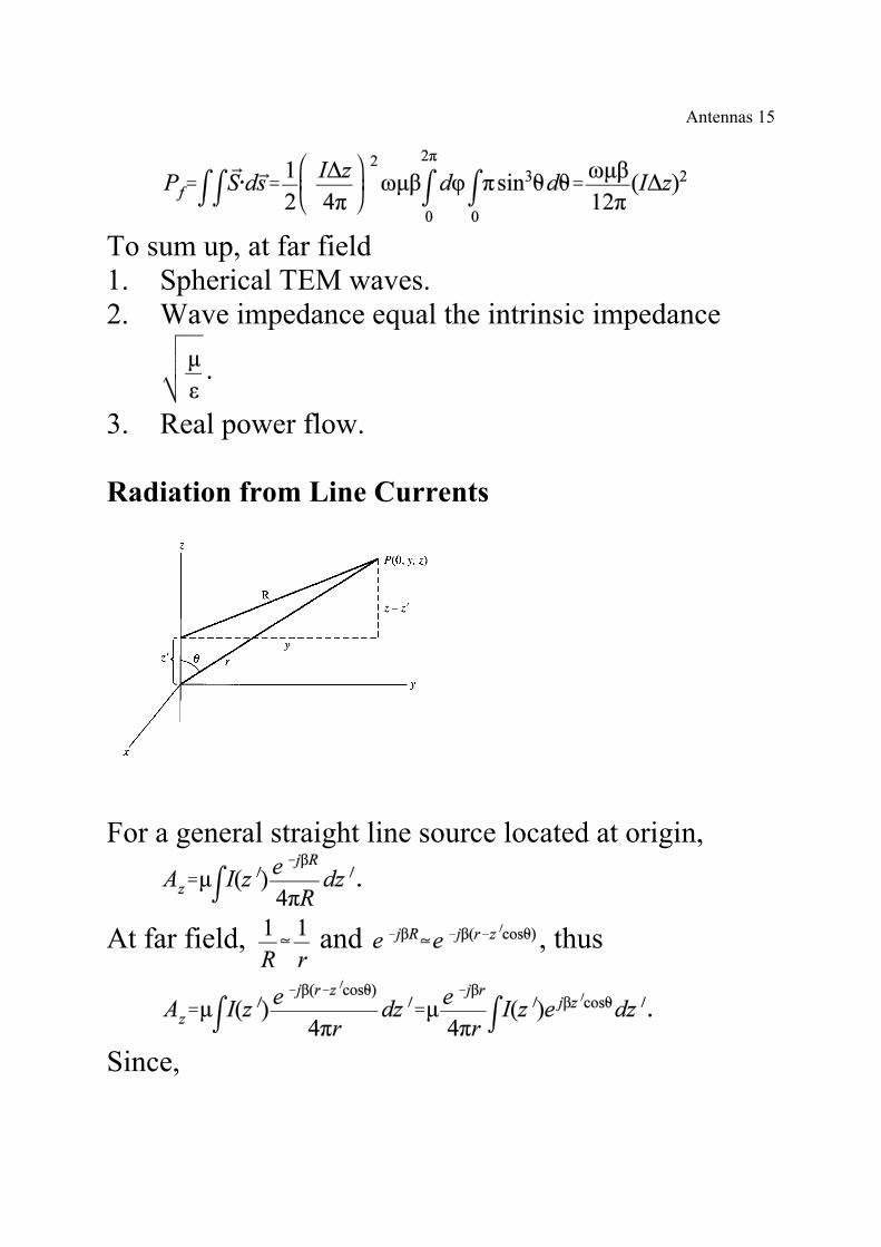
Radiation from Line Currents

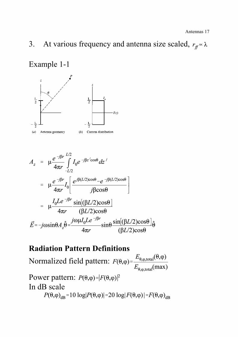
For a general straight line source located at origin,

.

At far field, and , thus

.

Since,

Antennas 16

At neglecting high order terms of ,

Similarly,

and

.

Far Field Conditions

To sum up:1. At fixed frequency, .

2. At fixed antenna size,

Antennas 17

3. At various frequency and antenna size scaled,

Example 1-1

Radiation Pattern Definitions

Normalized field pattern:

Power pattern: In dB scale

Antennas 18

ExamplesIdeal dipole:

Line current:

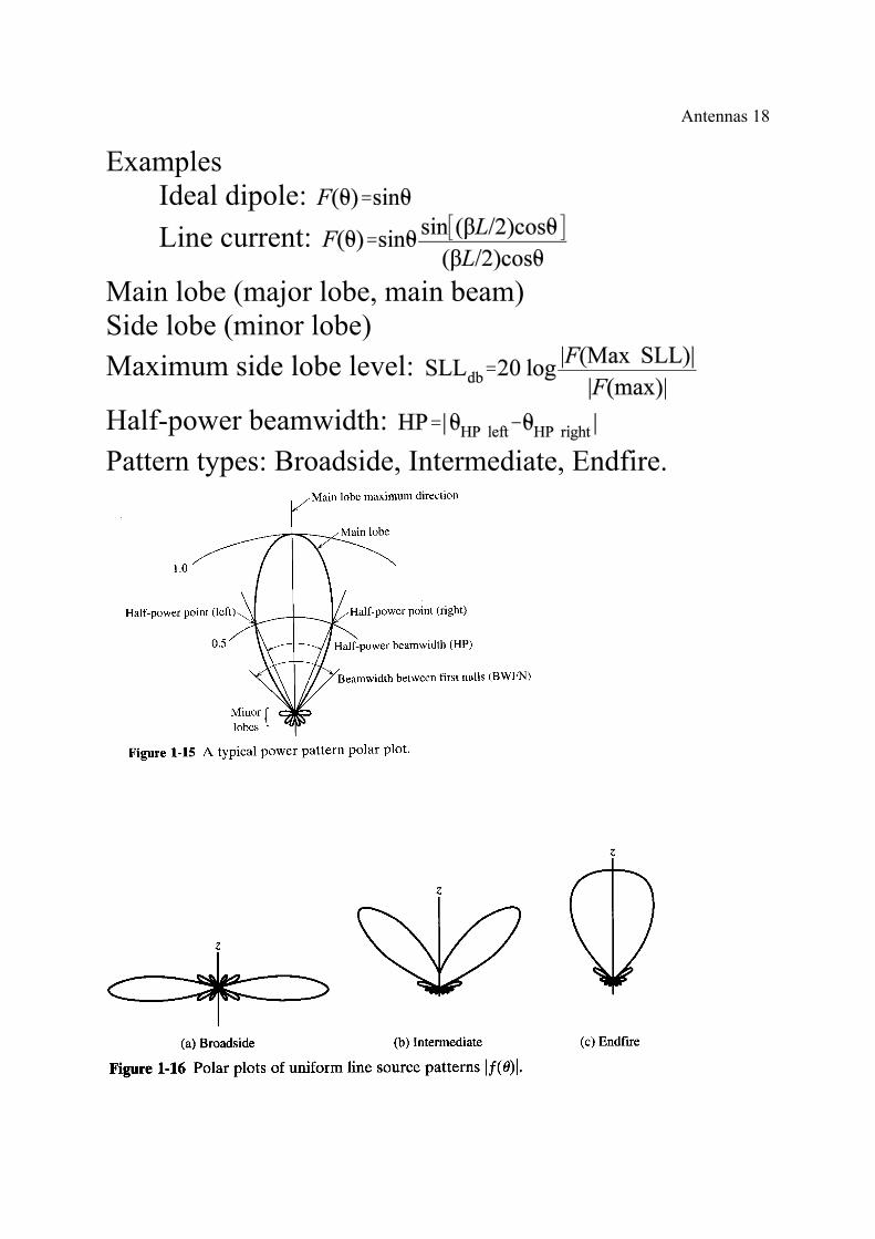
Main lobe (major lobe, main beam)Side lobe (minor lobe)Maximum side lobe level:

Half-power beamwidth:

Pattern types: Broadside, Intermediate, Endfire.

Antennas 19

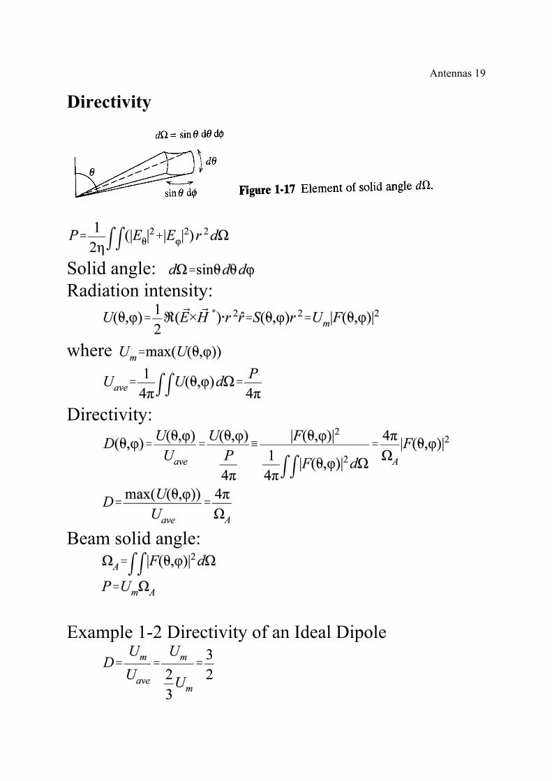
Directivity

Solid angle: Radiation intensity:

where

Directivity:

Beam solid angle:

Example 1-2 Directivity of an Ideal Dipole

Antennas 20

or

Example 1-3 Directivity of a Sector OmnidirectionalPattern

Power Gain (Gain)

or

Radiation efficiency:

Referenced Gain:

dBi: referenced to isotropic antenna.

Antennas 21

dBd: referenced to dipole antenna.

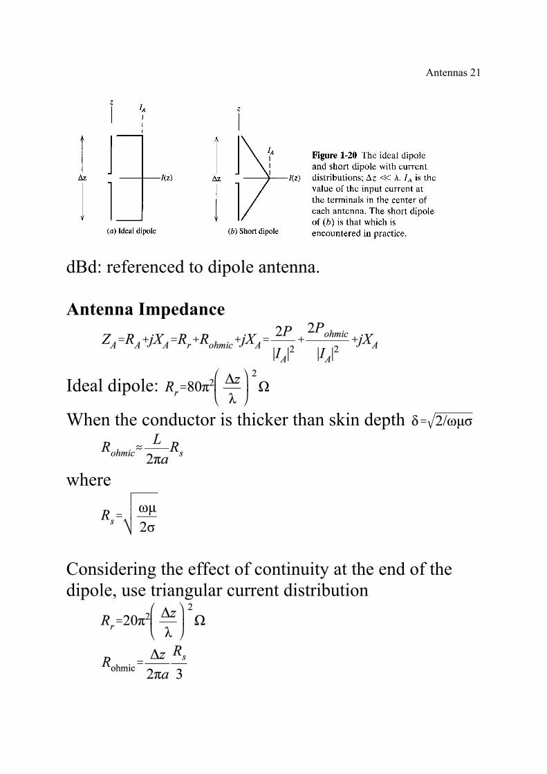
Antenna Impedance

Ideal dipole:

When the conductor is thicker than skin depth

where

Considering the effect of continuity at the end of thedipole, use triangular current distribution

Antennas 22

Example 1-4: Radiation Efficiency of an AM Car RadioAntenna.

Radius Dipole Length Frequency 1 MHz.

For short dipole,

Example 1-5: Input Reactance of an AM Car RadioAntenna of Example 1-4.

Antennas 23

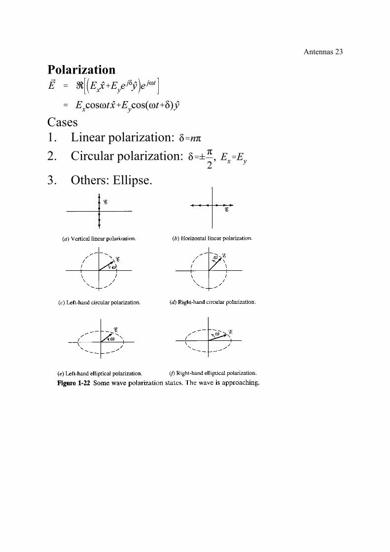
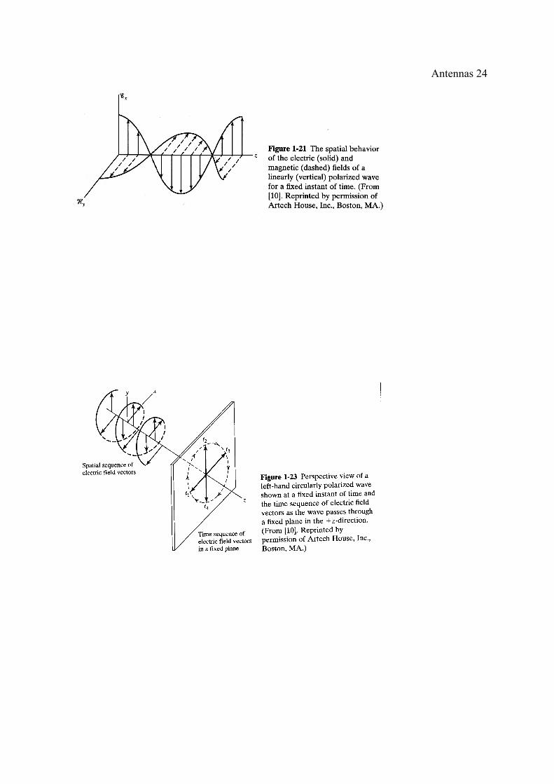
Polarization

Cases1. Linear polarization:

2. Circular polarization:

3. Others: Ellipse.

Antennas 24

Antennas 25

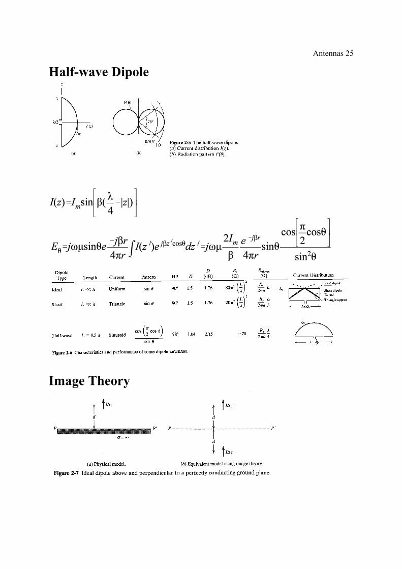
Half-wave Dipole

Image Theory

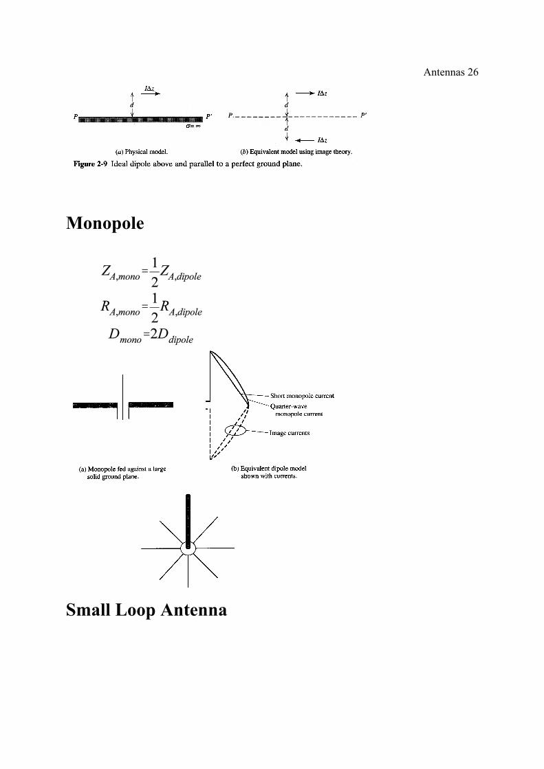
Antennas 26

Monopole

Small Loop Antenna

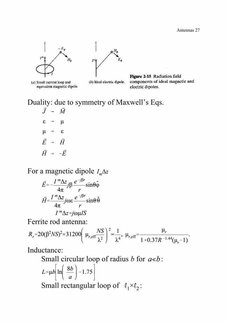
Antennas 27

Duality: due to symmetry of Maxwell’s Eqs.

For a magnetic dipole

Ferrite rod antenna:

Inductance:Small circular loop of radius b for :

Small rectangular loop of :

Antennas 28

Example 2-1: A Small Circular Loop AntennaLoop circumference Wire radius Frequency

Antennas 29

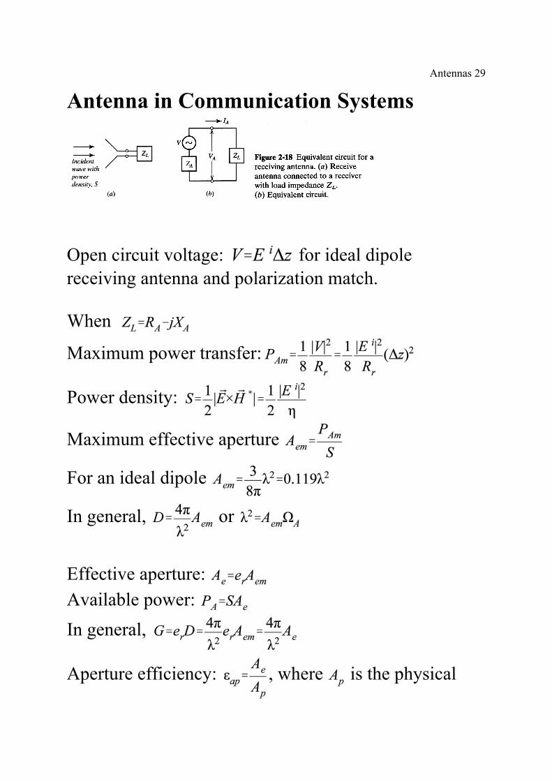
Antenna in Communication Systems

Open circuit voltage: for ideal dipolereceiving antenna and polarization match.

When

Maximum power transfer:

Power density:

Maximum effective aperture

For an ideal dipole

In general, or

Effective aperture:

Available power:

In general,

Aperture efficiency: , where is the physical

Antennas 30

aperture size.

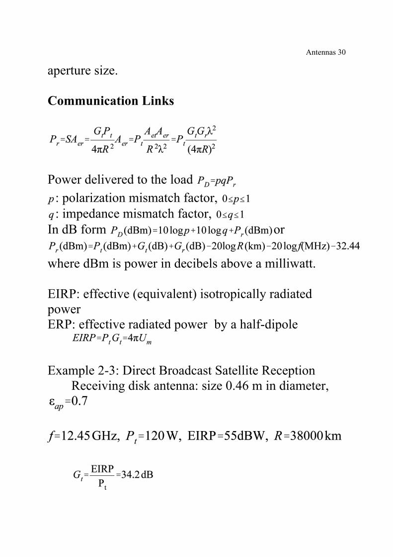
Communication Links

Power delivered to the load

: polarization mismatch factor, : impedance mismatch factor,

In dB form or

where dBm is power in decibels above a milliwatt.

EIRP: effective (equivalent) isotropically radiatedpowerERP: effective radiated power by a half-dipole

Example 2-3: Direct Broadcast Satellite ReceptionReceiving disk antenna: size 0.46 m in diameter,

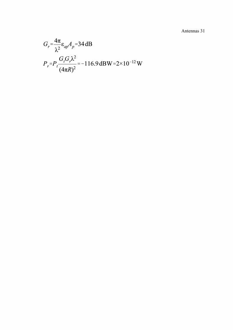
Antennas 31

Antennas 32

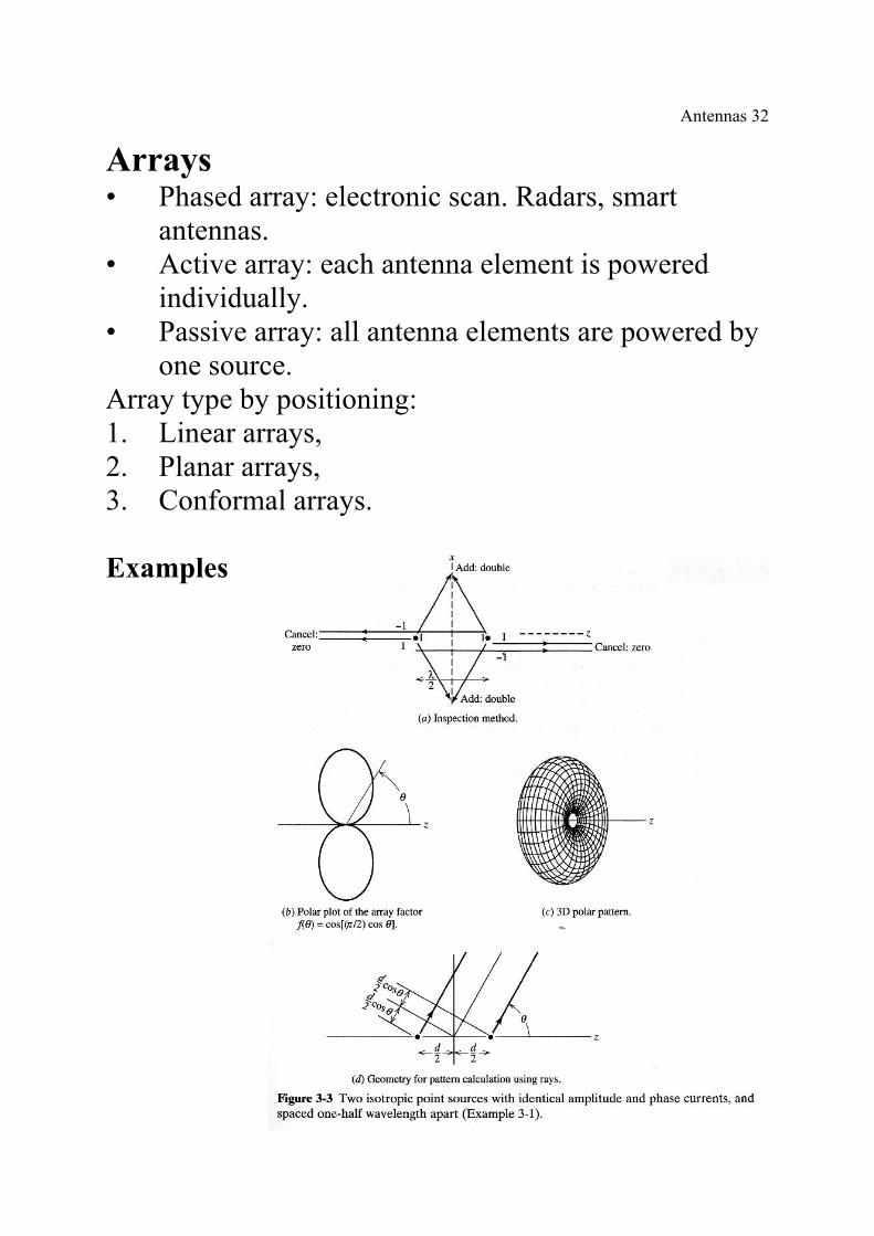
Arrays• Phased array: electronic scan. Radars, smart

antennas.• Active array: each antenna element is powered

individually.• Passive array: all antenna elements are powered by

one source.Array type by positioning:1. Linear arrays,2. Planar arrays,3. Conformal arrays.

Examples

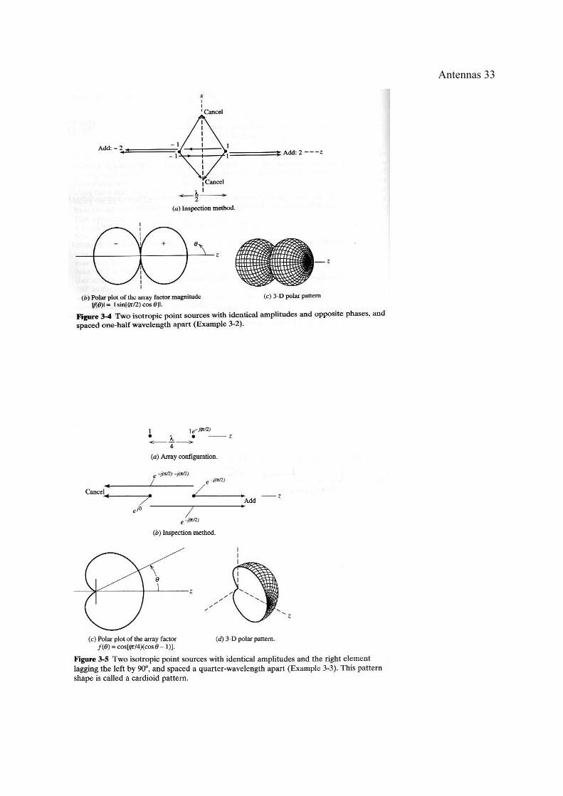
Antennas 33

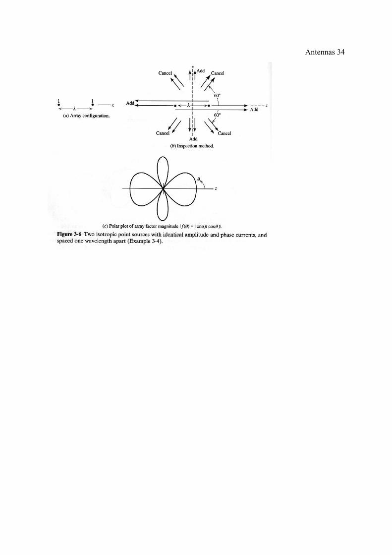
Antennas 34

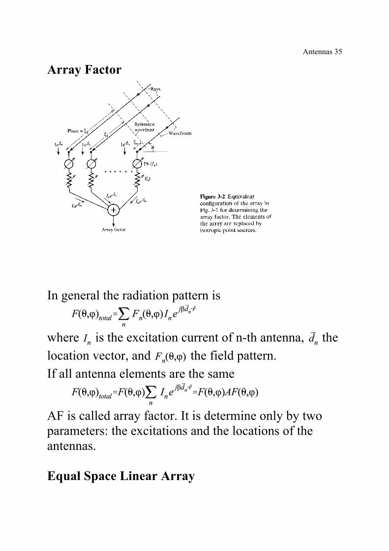
Antennas 35

Array Factor

In general the radiation pattern is

where is the excitation current of n-th antenna, the

location vector, and the field pattern.

If all antenna elements are the same

AF is called array factor. It is determine only by twoparameters: the excitations and the locations of theantennas.

Equal Space Linear Array

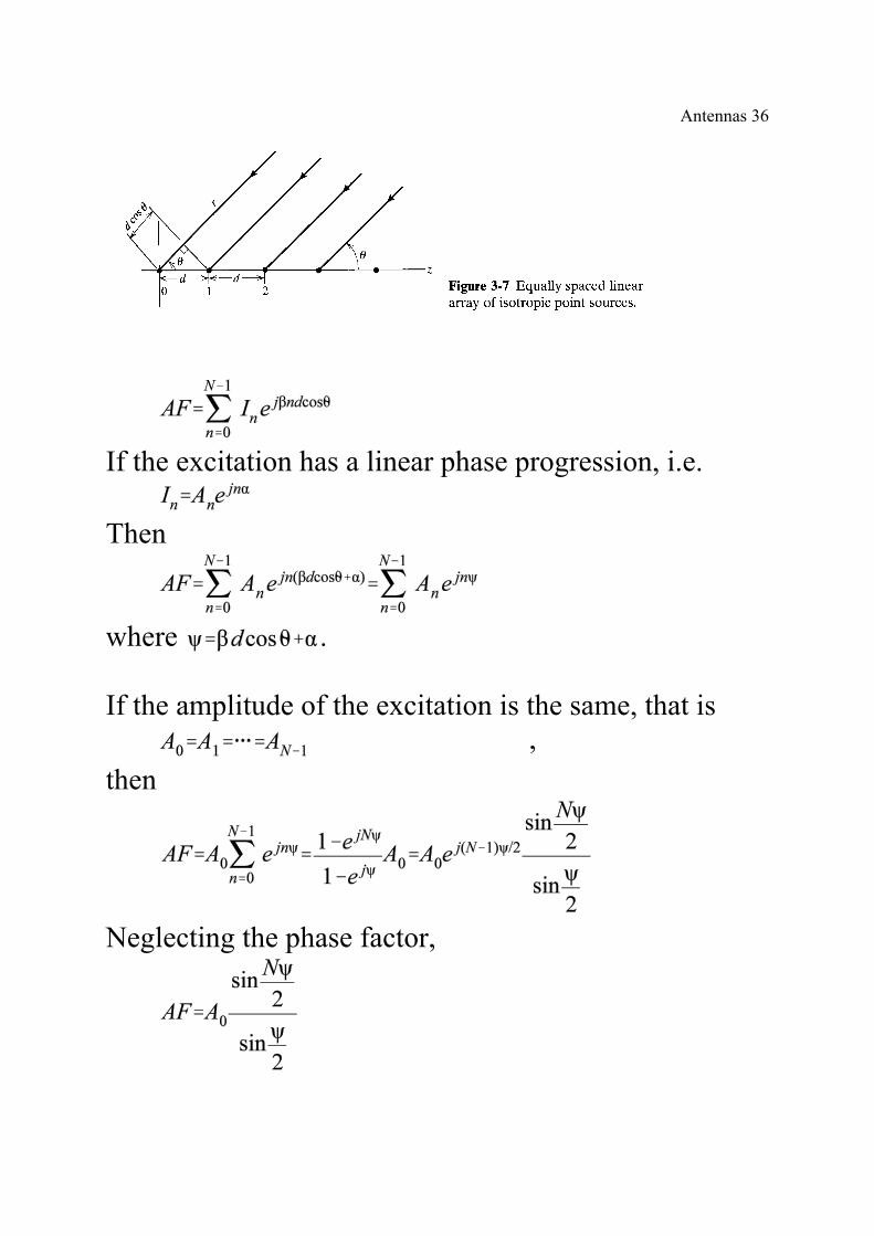
Antennas 36

If the excitation has a linear phase progression, i.e.

Then

where .

If the amplitude of the excitation is the same, that is,

then

Neglecting the phase factor,

Antennas 37

Normalized AF: .

Maximum at

Main beam at . This is the scanning effect.

Broadside: Endfire:

Summary:• N increases as the main lobe beamwidth decreases.• Number of side lobes: N-2.• Number of nulls: N-1.• Side lobe width: . Main lobe width: .• Side lobe peaks decrease with increasing N.• is symmetric about .

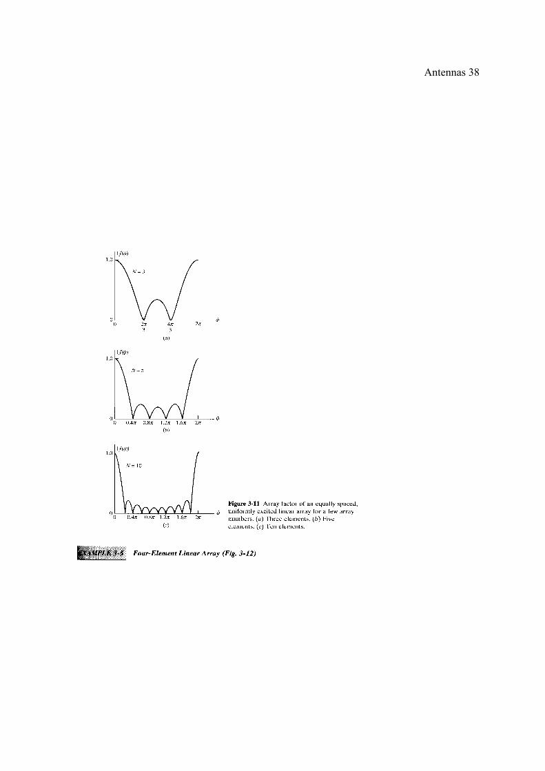
Antennas 38

Antennas 39

BWFN of Broadside Array ( )

First null occurs when , or

Then, for long array

Similarly, half power beamwidth near

broadside.

BWFN of Endfire ArrayFirst null occurs when , or

Similarly, half power beamwidth

Antennas 40

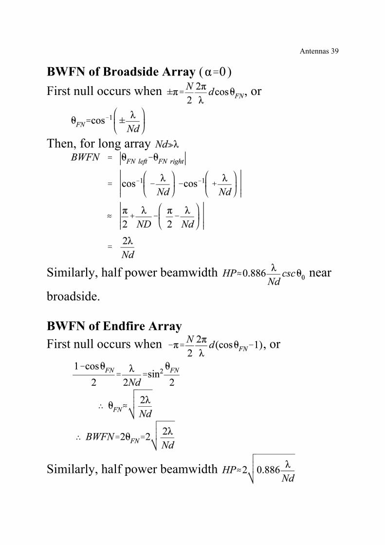
Example 3-5 Four-Element Linear ArrayParameters: , ,

Main beam

Antennas 41

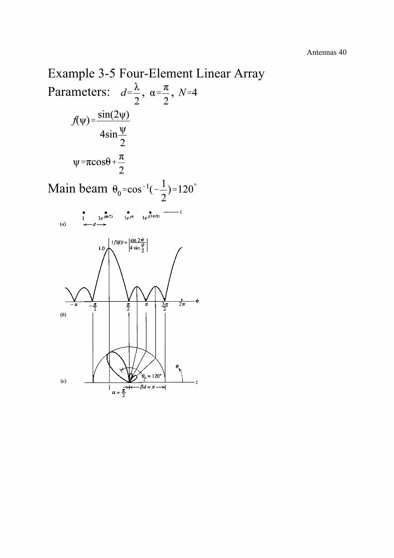
Single Mainbeam Oridinary Endfire ArrayOridinary Endfire: main beam at exactly or .Range of :

Half-width of a grating lobe:

Choose to eliminate most of the grating

lobe, or

Example 3-6 Five-Element Ordinary Endfire LinearArrayParameters:

Antennas 42

Hansen-Woodyard Endfire Array

Purpose: increase directivity by increasing to reducethe visible region of the main beam.Choose to reduce main beam width.Choose to prevent back lobe to becomelarger than main lobe.Maximum directivity for large array: .

Simpler Formula for :

Example 3-7 Five-Element Hansen-Woodyard EndfireLinear Array

Parameters: ,

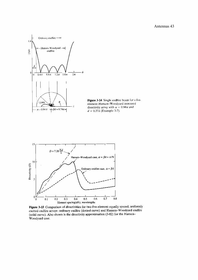
Antennas 43

Antennas 44

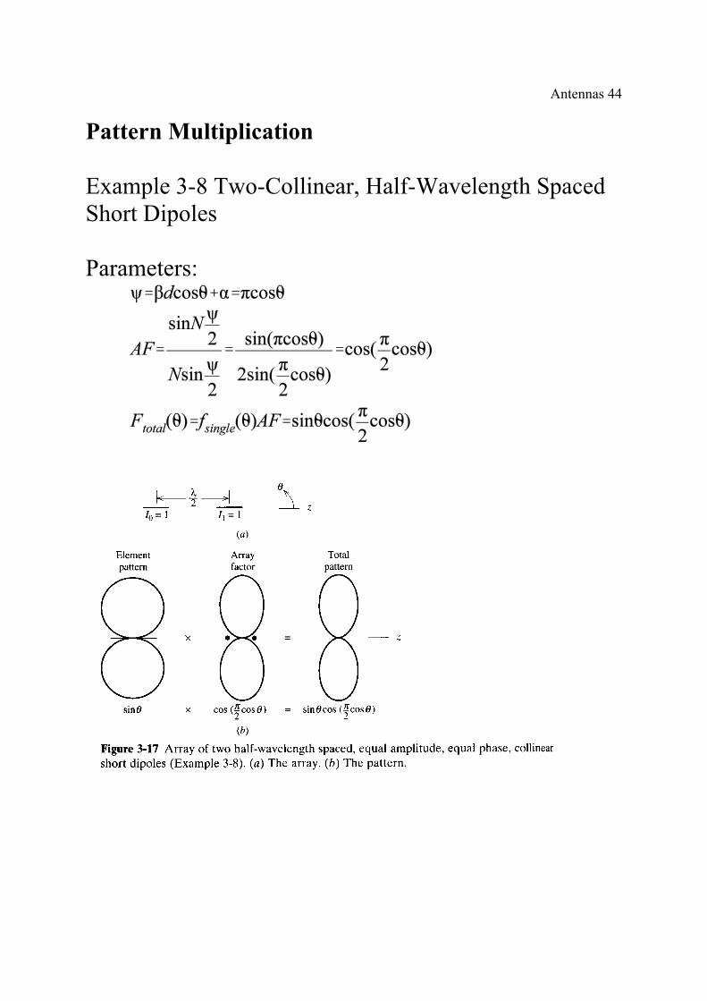
Pattern Multiplication

Example 3-8 Two-Collinear, Half-Wavelength SpacedShort Dipoles

Parameters:

Antennas 45

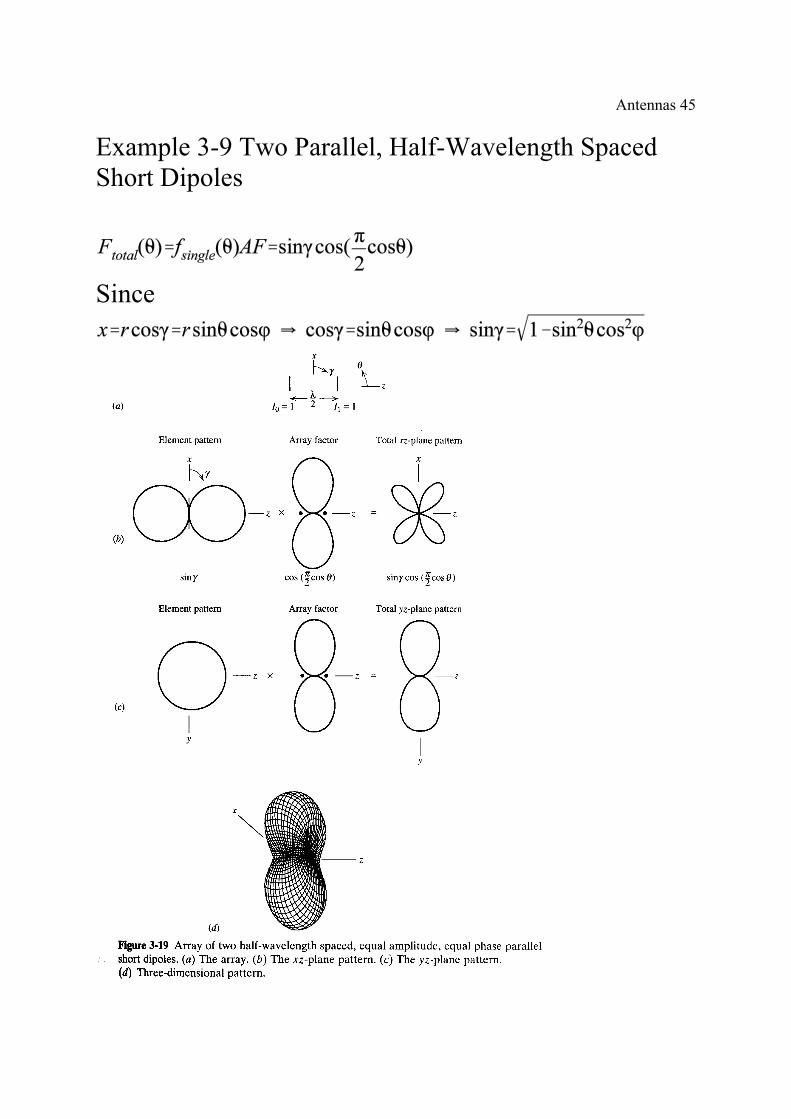
Example 3-9 Two Parallel, Half-Wavelength SpacedShort Dipoles

Since

Antennas 46

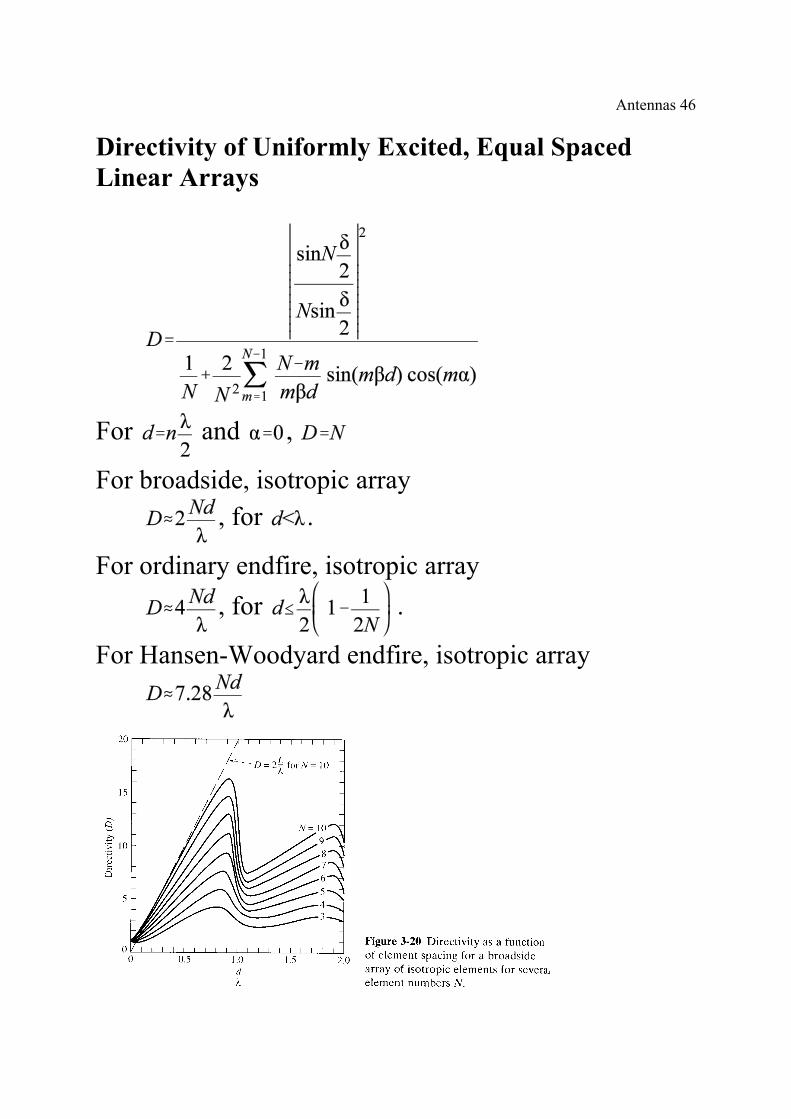
Directivity of Uniformly Excited, Equal SpacedLinear Arrays

For and ,

For broadside, isotropic array, for .

For ordinary endfire, isotropic array

, for .

For Hansen-Woodyard endfire, isotropic array

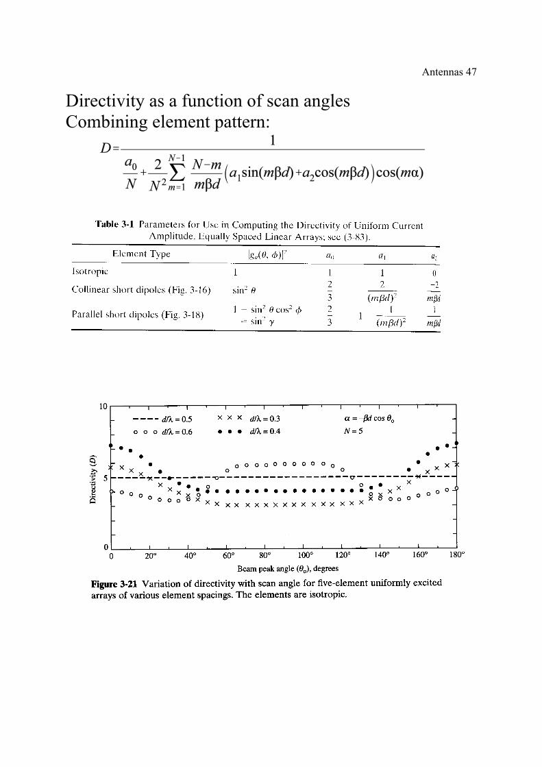
Antennas 47

Directivity as a function of scan anglesCombining element pattern:

Antennas 48

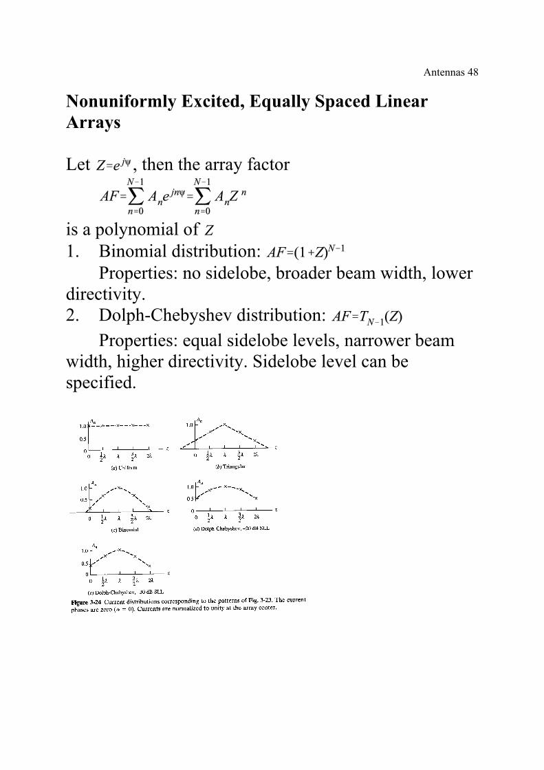
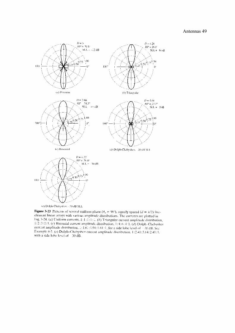
Nonuniformly Excited, Equally Spaced LinearArrays

Let , then the array factor

is a polynomial of 1. Binomial distribution:

Properties: no sidelobe, broader beam width, lowerdirectivity.2. Dolph-Chebyshev distribution:

Properties: equal sidelobe levels, narrower beamwidth, higher directivity. Sidelobe level can bespecified.

Antennas 49

Antennas 50

General expression of directivity of non-equal spacedand non-uniform excitation:

where is the current amplitude of k-th element, the

position, and .

For equal space, broadside array, , , we have

Furthermore, if , we have

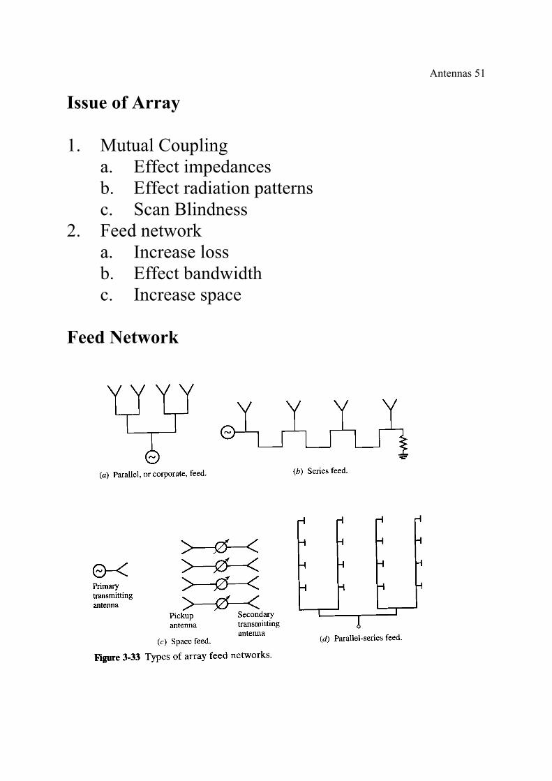
Antennas 51

Issue of Array

1. Mutual Couplinga. Effect impedancesb. Effect radiation patternsc. Scan Blindness

2. Feed networka. Increase lossb. Effect bandwidthc. Increase space

Feed Network

Antennas 52

Antennas 53

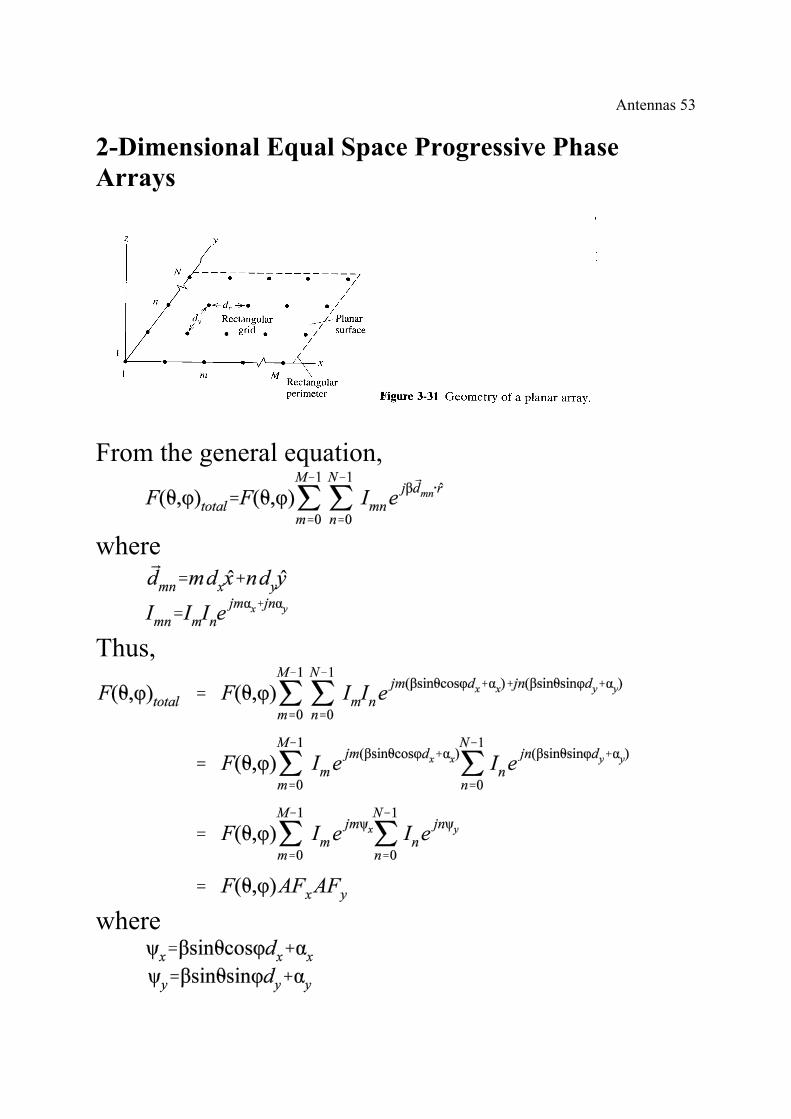
2-Dimensional Equal Space Progressive PhaseArrays

From the general equation,

where

Thus,

where

Antennas 54