Journal Identification = COMM Article Identification = 3055 Date: April 21, 2011 Time: 9:2 am

c o m p u t e r m e t h o d s a n d p r o g r a m s i n b i o m e d i c i n e 1 0 2 ( 2 0 1 1 ) 138–148

journa l homepage: www. int l .e lsev ierhea l th .com/ journa ls /cmpb

Anticipating the next meal using meal behavioral profiles:A hybrid model-based stochastic predictive controlalgorithm for T1DM�

C.S. Hughesa, S.D. Pateka,∗, M. Bretonb, B.P. Kovatcheva,b

a Department of Systems and Information Engineering, University of Virginia, United Statesb Department of Psychiatry and Neurobehavioral Sciences, University of Virginia, United States

a r t i c l e i n f o

Article history:

Received 14 December 2009

Received in revised form

26 March 2010

Accepted 27 April 2010

Keywords:

Diabetes

Artificial pancreas

Behavioral profiles

a b s t r a c t

Automatic control of Type 1 Diabetes Mellitus (T1DM) with subcutaneous (SC) measure-

ment of glucose concentration and subcutaneous (SC) insulin infusion is of great interest

within the diabetes technology research community. The main challenge with the so-called

“SC–SC” route to control is sensing and actuation delay, which tends to either destabilize the

system or inhibit the aggressiveness of the controller in responding to meals and exercise.

Model predictive control (MPC) is one strategy for mitigating delay, where optimal insulin

infusions can be given in anticipation of future meal disturbances. Unfortunately, exact

prior knowledge of meals can only be assured in a clinical environment and uncertainty

about when and if meals will arrive could lead to catastrophic outcomes. As a follow-on to

our recent paper in the IFAC symposium on Biological and Medical Systems (MCBMS 2009)

Linear quadratic Gaussian control

Model predictive control

[1], we develop a control law that can anticipate meals given a probabilistic description of

the patient’s eating behavior in the form of a random meal (behavioral) profile. Preclinical

in silico trials using the oral glucose meal model of Dalla Man et al. show that the control

strategy provides a convenient means of accounting for uncertain prior knowledge of meals

without compromising patient safety, even in the event that anticipated meals are skipped.

1. Introduction

Recent national data show that nearly 21 million Americans

have diabetes—a lifelong condition that affects people of everyage, race, and nationality, and is the leading cause of kid-ney failure, blindness, and amputations not related to injury.Approximately 1.5 million of these people have Type 1 Dia-

� This work was sponsored in part by (1) the Juvenile Diabetes ResearcLibrary of Medicine (Award Number T15LM009462). This content is srepresent the official views of the JDRF, the National Library of MedFoundation (NSF) grant CNS-0931633 and the National Institutes of Hea

∗ Corresponding author at: Department of Systems and Information EngiCharlottesville, VA 22904, United States. Tel.: +1 4349822052.

E-mail address: patek@virginia.edu (S.D. Patek).0169-2607/$ – see front matter © 2010 Elsevier Ireland Ltd. All rights resdoi:10.1016/j.cmpb.2010.04.011

© 2010 Elsevier Ireland Ltd. All rights reserved.

betes Mellitus (T1DM), in which the immune system destroysthe pancreatic beta cells, permanently suppressing insulinsecretion. A typical T1DM patient will need 50,000 insulinshots over his/her lifetime, accompanied by testing of blood

h Foundation (JDRF) Artificial Pancreas Project and (2) the Nationalolely the responsibility of the authors and does not necessarilyicine, or the National Institutes of Health the National Sciencelth (NIH) grant NIH/NIDDK-RO1-DK085623.neering, University of Virginia, 151 Engineers Way, P.O. Box 400747,

glucose levels several times a day. Automatic control of bloodglucose has been studied for more than three decades andwidely different solutions have been proposed. We refer to[2,3] for a review of the early literature, most of which focuses

erved.

Journal Identification = COMM Article Identification = 3055 Date: April 21, 2011 Time: 9:2 am

i n b i

oac

lbiGtimbssotlcat

meapaemopimtl

poiilaraTcpwr

ctdweitnuec

follows:

x(k + 1) = Ax(k) + Bu(k) + Gω(k) (1)

c o m p u t e r m e t h o d s a n d p r o g r a m s

n the case of intravenous (IV) glucose measurement and IVctuation, with both positive (glucose) and negative (insulin)ontrol variables.

As an extension to [1], this paper addresses the chal-enge to develop effective closed loop systems for regulatinglood glucose concentration, via the “SC–SC” route to control,.e. using commercially available subcutaneous Continuouslucose Monitoring (CGM) sensors and conventional subcu-

aneous insulin pump devices. The SC–SC control problems more challenging than control with intravenous measure-

ent of glucose and insulin infusion, for several reasons. First,ecause measurement and actuation are achieved via inter-titial fluids (and not directly in the bloodstream) there areignificant delays associated with this mode of control. Statef the art CGM technology relies on sensing glucose in intersti-ial fluids, which reflects blood glucose with an unknown timeag (between 0 and 45 min [4–6]). Also, the delay introduced byonventional (interstitial) insulin infusion pumps can lead tolimit on control performance, hindering the system’s ability

o reject major disturbances, specifically meals and exercise.Model Predictive Control (MPC) has been proposed as a

eans of overcoming measurement and actuation delay inither IV- or SC-based systems, cf. [2,7,8], where controlctions are computed at update intervals based on modelredicted optimal future evolution of the system taking intoccount knowledge about future disturbances. While clinicalvaluation of these algorithms is underway, there are clearlyany obstacles to automated control of blood glucose outside

f the clinic, including the need for on-going adaptation to theatient’s time-varying physiological parameters and behav-

or. In this work we address this issue by developing a controlethodology that plans insulin delivery given a probabilis-

ic model of meal timing and meal amounts, which can beearned from historical data.

Run-to-run control methods adopted from the chemicalrocess control literature have also been proposed as a meansf responding to time-varying aspects of the patient’s behav-

or and physiology. Recent studies have shown that, even withnfrequent sampling of blood glucose, run-to-run control canearn bolus and basal rate profiles that are optimal (on aver-ge) in the face of time-varying aspects of the patient’s dailyoutine (e.g. timing of meals), cf. [9–11], and circadian fluctu-tion in insulin resistance (e.g. dawn phenomenon), cf. [12].he approach developed in this paper differs from run-to-runontrol in that it employs an explicit probabilistic model ofatient meal behavior (including the possibility that the mealill be skipped) and accordingly plans a model-based dynamic

esponse to both measured glucose and anticipated meals.To outline the sequel, in Section 2, we derive a general

ontrol law that optimizes an expected quadratic cost cri-erion for a linear system subject to a random single shockisturbance, which for this paper represents a potential mealith unknown timing. We set up our Shock-Anticipating Lin-

ar Quadratic Regulator (SA-LQR) methodology in Section 3,ntroducing the notion of a random meal profile characterizinghe likelihood, timing, and carbohydrate (CHO) content of the

ext meal and reviewing the glucose–insulin kinetics modelsed to derive our control law, where state observation ismployed. Section 3 also describes a hybrid open-closed loopontrol strategy, where a closed loop control is used in antic-

o m e d i c i n e 1 0 2 ( 2 0 1 1 ) 138–148 139

ipation of meal arrival, while a meal bolus which is informedby insulin-on-board is delivered at the time of meal arrival.In Section 4, we illustrate the benefits of our control strat-egy for a breakfast meal scenario. We focus in Section 4 oncontroller performance in cases where the anticipated mealfails to arrive. Throughout, we focus exclusively on the useof insulin for managing blood glucose concentration, ignor-ing the opportunity to infuse other metabolic hormones suchas glucagon, which can provide a so-called “positive” controleffect; however, our control methodology can be extended tothis setting provided a suitable model of glucagon effect. InSection 5, we compare the SA-LQR strategy to an open loopconventional therapy approach, in which we deliver basal ratecontinuously and a meal bolus at mealtime. In Section 6, wewrap up the paper with brief conclusions and directions forfuture work. Finally, we prove the main technical result intro-duced in Section 2 in the Appendix.

2. Anticipating “shock” disturbances;shock-anticipating LQR (SA-LQR)

In the context of control of T1DM, meals are the primary dis-turbance. These meal disturbances occur at random timeswith random magnitudes and can be treated as “shock” dis-turbances.

Here, we derive a generic optimal linear quadratic con-trol law that anticipates a single random “shock” disturbancethat, if it arrives at all, will arrive in stages k = 0 through k̄.The setup here is general: we assume that the plant is lin-ear, time-invariant, with x(k) ∈ �nx , u(k) ∈ �nu , and ω(k) ∈ �nd .Let d̃ + w ∈ �nd denote the “shock disturbance,” which arrives(or not) according to the conditional probability of arrival pk

given that the shock has not arrived prior to stage k ∈ {0, . . . , k̄},where d̃ is deterministic and w is a zero-mean perturbation.1

Models of this type have been studied before. Perhaps theclosest related work can be found in [13], which addressesfinite-horizon, stochastic hybrid systems, subject to Marko-vian jump parameters. (We pose an infinite horizon problem,where the “shock” disturbance is distinctly non-Markovian.)The control law is designed to minimize expected quadraticcost associated with state and control deviations away fromtarget levels, where the conditional probabilities of mealarrival pk factor into an anticipatory effect prior to thenext meal.

We assume that the controller is aware of the “shock” dis-turbance when it arrives, and consequently we augment thestate vector x(k) of the dynamical system (18) with an addi-tional “disturbance state” m(k) that provides an indicationof whether the disturbance is still possible (m(k) = 0 if “yes,”m(k) = 1 if “no”). The augmented dynamical equations are as

1 In the context of control of T1DM, pk becomes the probabilitythat the meal will “arrive” in stage k, given that the meal has notyet occurred (this is discussed in more detail in Section 3).

Journal Identification = COMM Article Identification = 3055 Date: April 21, 2011 Time: 9:2 am

s i n

140 c o m p u t e r m e t h o d s a n d p r o g r a m

m(k + 1) = max{m(k), Ik} (2)

where Ik is the indictor variable for the event that the shockarrives in stage k and the initial state of the process is(x(0), m(0)) = (x, 0) for any initial state space vector x. In prac-tice, the transition from m(k) = 0 to m(k + 1) = 1 (i.e. ω(k) /= 0or k = k̄) would be observed. (In the context of blood glucosecontrol, the patient would either press a “meal now” button ora meal detection algorithm would provide such an indication.)We set as a control objective the expected value of a quadraticfunctional involving both state errors and control utilization:

J(x(0), m(0)) = E

{ ∞∑t=0

[x(t)′Qx(t) + u(t)′Ru(t)]

}(3)

where Q and R are both symmetric and positive semidefiniteand positive definite, respectively. Let C denote the “squareroot” of Q, such that Q = C′C. Also, for notational conveniencein the sequel, let

J∗k(x, m) ≡ min E

{ ∞∑t=k

[x(t)′Qx(t) + u(t)′Ru(t)]

}(4)

where the expectation above is conditional on x(k) = x andm(k) = m. For states where m(k) = 1 the shock disturbance isno longer possible, and the problem of minimizing the infi-nite horizon quadratic cost-to-go amounts to a standard LQRproblem. However, for states where m(k) = 0 the shock mayarrive at some future time, and the minimization of expectedquadratic costs involves an optimal response in anticipation ofthe disturbance. The basic idea is:

J∗k(x, 1) = optimal LQR cost-to-go from x,

with no more future disturbances = x′Px

and

J∗k(x, 0) = optimal cost-to-go from x, with anticipation of a

possible future disturbance= min

u[E[pkJk+1(Ax + Bu + Gd̃, 1)]]

+ [[(1 − pk)Jk+1(Ax + Bu, 0)]]

The following proposition establishes the form of both J∗k(x, m)

and the optimal control law in detail.

Proposition 1. Given that the pair (A, B) is controllable and the pair(A, C) is observable, the optimal control law is uniquely characterizedas follows:

(1) At states where m(k) = 1,

J∗k(x, 1) = x′Px (5)

and the minimizing control action at state (x, 1) in stage k is

u∗k(x, 1) = −Kx (6)

b i o m e d i c i n e 1 0 2 ( 2 0 1 1 ) 138–148

where P is the unique positive semidefinite solution to the Riccatiequation

P = A′(P − PB�−1B′P)A + Q (7)

with � = R + B′PB, and K = �−1B′PA.(2) At states where m(k) = 0, the optimal expected cost-to-go func-

tion takes the form

J∗k(x, 0) = x′Px + d̃′Hkx + d̃′Lkd̃ + �k (8)

and the minimizing control action at state (x, 0) in stage k is

u∗k(x, 0) = −Kx − K̃kd̃ (9)

where Hk, Lk, �k, and K̃k, is derived from the following(3) Backwards recursion:

(a) Stage k = k̄:

K̃k̄

= pk̄�−1B′PG (10)

Hk̄

= G′[2pk̄P − 2p

k̄PB�−1B′P]A (11)

Lk̄

= G′[pk̄P − p2

k̄PB�−1B′P]G (12)

�k̄

= pk̄Ew((Gw̃)′P(Dw̃)) (13)

(b) Stage k < k̄:

K̃k = �−1B′Qk (14)

Hk = 2Q ′k(I − B�−1B′P)A (15)

Lk = pkG′PG + qkLk+1 − Q ′kB�−1B′Qk (16)

�k = pkEw[w′G′PGw] + qk�k+1 (17)

where Qk = (1 − pk)(Hk+1)′/2 + pkPG.

The proof of the proposition employs familiar techniquesused in the analysis of linear-quadratic control models. Werefer to the Appendix B for the formal arguments.

3. SA-LQR with behavioral profiles

Our control strategy is motivated from the realization that his-torical data about a patient’s eating behavior can be used tocharacterize the timing and likelihood of a meal disturbancewithin pre-specified meal regimes (e.g. breakfast), along withthe magnitude of the disturbance. We refer for example to [14],which outlines a method for establishing a probabilistic meal-pattern profile for individuals based on CGM data. “Profile”information can be used in planning insulin injections prior

to the arrival of meals, as long as the uncertainties involvedare appropriately considered. In Section 3.4 we also formulatean insulin-informed control action to be taken at the time ofthe disturbance arrival.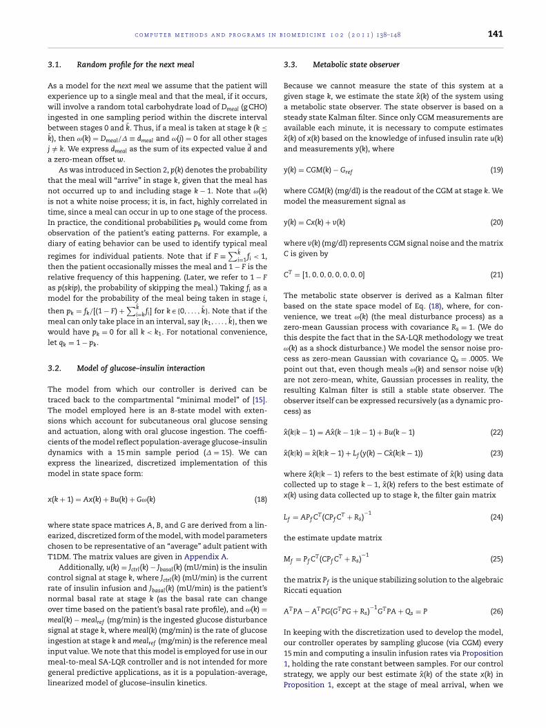

Journal Identification = COMM Article Identification = 3055 Date: April 21, 2011 Time: 9:2 am

i n b i

3

Aewibk

j

a

tnitIod

rtram

tmwl

3

TtTsacdem

x

wecT

crnom

siimgl

c o m p u t e r m e t h o d s a n d p r o g r a m s

.1. Random profile for the next meal

s a model for the next meal we assume that the patient willxperience up to a single meal and that the meal, if it occurs,ill involve a random total carbohydrate load of Dmeal (g CHO)

ngested in one sampling period within the discrete intervaletween stages 0 and k̄. Thus, if a meal is taken at stage k (k ≤

¯ ), then ω(k) = Dmeal/� ≡ dmeal and ω(j) = 0 for all other stages/= k. We express dmeal as the sum of its expected value d̃ andzero-mean offset w.

As was introduced in Section 2, p(k) denotes the probabilityhat the meal will “arrive” in stage k, given that the meal hasot occurred up to and including stage k − 1. Note that ω(k)

s not a white noise process; it is, in fact, highly correlated inime, since a meal can occur in up to one stage of the process.n practice, the conditional probabilities pk would come frombservation of the patient’s eating patterns. For example, aiary of eating behavior can be used to identify typical meal

egimes for individual patients. Note that if F ≡ ∑k̄

i=1fi < 1,hen the patient occasionally misses the meal and 1 − F is theelative frequency of this happening. (Later, we refer to 1 − F

s p(skip), the probability of skipping the meal.) Taking fi as aodel for the probability of the meal being taken in stage i,

hen pk = fk/[(1 − F) +∑k̄

i=kfi] for k ∈ {0, . . . , k̄}. Note that if the

eal can only take place in an interval, say {k1, . . . , k̄}, then weould have pk = 0 for all k < k1. For notational convenience,

et qk = 1 − pk.

.2. Model of glucose–insulin interaction

he model from which our controller is derived can beraced back to the compartmental “minimal model” of [15].he model employed here is an 8-state model with exten-ions which account for subcutaneous oral glucose sensingnd actuation, along with oral glucose ingestion. The coeffi-ients of the model reflect population-average glucose–insulinynamics with a 15 min sample period (� = 15). We canxpress the linearized, discretized implementation of thisodel in state space form:

(k + 1) = Ax(k) + Bu(k) + Gω(k) (18)

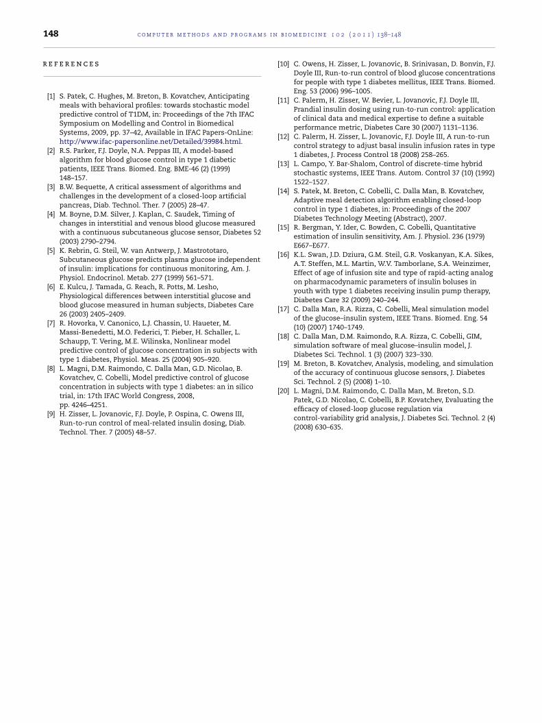
here state space matrices A, B, and G are derived from a lin-arized, discretized form of the model, with model parametershosen to be representative of an “average” adult patient with1DM. The matrix values are given in Appendix A.

Additionally, u(k) = Jctrl(k) − Jbasal(k) (mU/min) is the insulinontrol signal at stage k, where Jctrl(k) (mU/min) is the currentate of insulin infusion and Jbasal(k) (mU/min) is the patient’sormal basal rate at stage k (as the basal rate can changever time based on the patient’s basal rate profile), and ω(k) =eal(k) − mealref (mg/min) is the ingested glucose disturbance

ignal at stage k, where meal(k) (mg/min) is the rate of glucosengestion at stage k and mealref (mg/min) is the reference meal

nput value. We note that this model is employed for use in our

eal-to-meal SA-LQR controller and is not intended for moreeneral predictive applications, as it is a population-average,inearized model of glucose–insulin kinetics.

o m e d i c i n e 1 0 2 ( 2 0 1 1 ) 138–148 141

3.3. Metabolic state observer

Because we cannot measure the state of this system at agiven stage k, we estimate the state x̂(k) of the system usinga metabolic state observer. The state observer is based on asteady state Kalman filter. Since only CGM measurements areavailable each minute, it is necessary to compute estimatesx̂(k) of x(k) based on the knowledge of infused insulin rate u(k)and measurements y(k), where

y(k) = CGM(k) − Gref (19)

where CGM(k) (mg/dl) is the readout of the CGM at stage k. Wemodel the measurement signal as

y(k) = Cx(k) + v(k) (20)

where v(k) (mg/dl) represents CGM signal noise and the matrixC is given by

CT = [1, 0, 0, 0, 0, 0, 0, 0] (21)

The metabolic state observer is derived as a Kalman filterbased on the state space model of Eq. (18), where, for con-venience, we treat ω(k) (the meal disturbance process) as azero-mean Gaussian process with covariance Rs = 1. (We dothis despite the fact that in the SA-LQR methodology we treatω(k) as a shock disturbance.) We model the sensor noise pro-cess as zero-mean Gaussian with covariance Qs = .0005. Wepoint out that, even though meals ω(k) and sensor noise v(k)are not zero-mean, white, Gaussian processes in reality, theresulting Kalman filter is still a stable state observer. Theobserver itself can be expressed recursively (as a dynamic pro-cess) as

x̂(k|k − 1) = Ax̂(k − 1|k − 1) + Bu(k − 1) (22)

x̂(k|k) = x̂(k|k − 1) + Lf (y(k) − Cx̂(k|k − 1)) (23)

where x̂(k|k − 1) refers to the best estimate of x̂(k) using datacollected up to stage k − 1, x̂(k) refers to the best estimate ofx(k) using data collected up to stage k, the filter gain matrix

Lf = APf CT(CPf CT + Rs)−1

(24)

the estimate update matrix

Mf = Pf CT(CPf CT + Rs)−1

(25)

the matrix Pf is the unique stabilizing solution to the algebraicRiccati equation

ATPA − ATPG(GTPG + Rs)−1

GTPA + Qs = P (26)

In keeping with the discretization used to develop the model,our controller operates by sampling glucose (via CGM) every

15 min and computing a insulin infusion rates via Proposition1, holding the rate constant between samples. For our controlstrategy, we apply our best estimate x̂(k) of the state x(k) inProposition 1, except at the stage of meal arrival, when we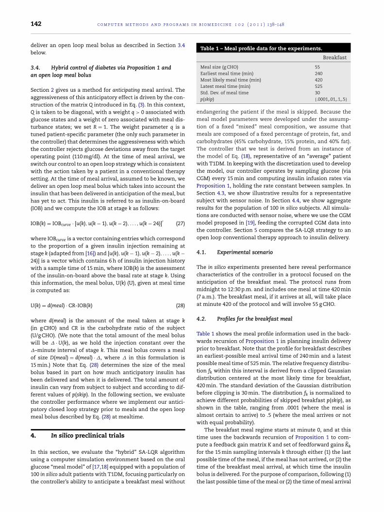

Journal Identification = COMM Article Identification = 3055 Date: April 21, 2011 Time: 9:2 am

s i n b i o m e d i c i n e 1 0 2 ( 2 0 1 1 ) 138–148

Table 1 – Meal profile data for the experiments.

Breakfast

Meal size (g CHO) 55Earliest meal time (min) 240

142 c o m p u t e r m e t h o d s a n d p r o g r a m

deliver an open loop meal bolus as described in Section 3.4below.

3.4. Hybrid control of diabetes via Proposition 1 andan open loop meal bolus

Section 2 gives us a method for anticipating meal arrival. Theaggressiveness of this anticipatory effect is driven by the con-struction of the matrix Q introduced in Eq. (3). In this context,Q is taken to be diagonal, with a weight q > 0 associated withglucose states and a weight of zero associated with meal dis-turbance states; we set R = 1. The weight parameter q is atuned patient-specific parameter (the only such parameter inthe controller) that determines the aggressiveness with whichthe controller rejects glucose deviations away from the targetoperating point (110 mg/dl). At the time of meal arrival, weswitch our control to an open loop strategy which is consistentwith the action taken by a patient in a conventional therapysetting. At the time of meal arrival, assumed to be known, wedeliver an open loop meal bolus which takes into account theinsulin that has been delivered in anticipation of the meal, buthas yet to act. This insulin is referred to as insulin-on-board(IOB) and we compute the IOB at stage k as follows:

IOB(k) = IOBcurve · [u(k), u(k − 1), u(k − 2), . . . , u(k − 24)]′ (27)

where IOBcurve is a vector containing entries which correspondto the proportion of a given insulin injection remaining atstage k (adapted from [16]) and [u(k), u(k − 1), u(k − 2), . . . , u(k −24)] is a vector which contains 6 h of insulin injection historywith a sample time of 15 min, where IOB(k) is the assessmentof the insulin-on-board above the basal rate at stage k. Usingthis information, the meal bolus, U(k) (U), given at meal timeis computed as:

U(k) = d(meal) · CR-IOB(k) (28)

where d(meal) is the amount of the meal taken at stage k(in g CHO) and CR is the carbohydrate ratio of the subject(U/g CHO). (We note that the total amount of the meal boluswill be � · U(k), as we hold the injection constant over the�–minute interval of stage k. This meal bolus covers a mealof size D(meal) = d(meal) · �, where � in this formulation is15 min.) Note that Eq. (28) determines the size of the mealbolus based in part on how much anticipatory insulin hasbeen delivered and when it is delivered. The total amount ofinsulin can vary from subject to subject and according to dif-ferent values of p(skip). In the following section, we evaluatethe controller performance where we implement our antici-patory closed loop strategy prior to meals and the open loopmeal bolus described by Eq. (28) at mealtime.

4. In silico preclinical trials

In this section, we evaluate the “hybrid” SA-LQR algorithm

using a computer simulation environment based on the oralglucose “meal model” of [17,18] equipped with a population of100 in silico adult patients with T1DM, focusing particularly onthe controller’s ability to anticipate a breakfast meal without

Most likely meal time (min) 420Latest meal time (min) 525Std. Dev. of meal time 30p(skip) {.0001,.01,.1,.5}

endangering the patient if the meal is skipped. Because themeal model parameters were developed under the assump-tion of a fixed “mixed” meal composition, we assume thatmeals are composed of a fixed percentage of protein, fat, andcarbohydrates (45% carbohydrate, 15% protein, and 40% fat).The controller that we test is derived from an instance ofthe model of Eq. (18), representative of an “average” patientwith T1DM. In keeping with the discretization used to developthe model, our controller operates by sampling glucose (viaCGM) every 15 min and computing insulin infusion rates viaProposition 1, holding the rate constant between samples. InSection 4.3, we show illustrative results for a representativesubject with sensor noise. In Section 4.4, we show aggregateresults for the population of 100 in silico subjects. All simula-tions are conducted with sensor noise, where we use the CGMmodel proposed in [19], feeding the corrupted CGM data intothe controller. Section 5 compares the SA-LQR strategy to anopen loop conventional therapy approach to insulin delivery.

4.1. Experimental scenario

The in silico experiments presented here reveal performancecharacteristics of the controller in a protocol focused on theanticipation of the breakfast meal. The protocol runs frommidnight to 12:30 p.m. and includes one meal at time 420 min(7 a.m.). The breakfast meal, if it arrives at all, will take placeat minute 420 of the protocol and will involve 55 g CHO.

4.2. Profiles for the breakfast meal

Table 1 shows the meal profile information used in the back-wards recursion of Proposition 1 in planning insulin deliveryprior to breakfast. Note that the profile for breakfast describesan earliest-possible meal arrival time of 240 min and a latestpossible meal time of 525 min. The relative frequency distribu-tion fk within this interval is derived from a clipped Gaussiandistribution centered at the most likely time for breakfast,420 min. The standard deviation of the Gaussian distributionbefore clipping is 30 min. The distribution fk is normalized toachieve different probabilities of skipped breakfast p(skip), asshown in the table, ranging from .0001 (where the meal isalmost certain to arrive) to .5 (where the meal arrives or notwith equal probability).

The breakfast meal regime starts at minute 0, and at thistime uses the backwards recursion of Proposition 1 to com-pute a feedback gain matrix K and set of feedforward gains K̃k

for the 15 min sampling intervals k through either (1) the last

possible time of the meal, if the meal has not arrived, or (2) thetime of the breakfast meal arrival, at which time the insulinbolus is delivered. For the purpose of comparison, following (1)the last possible time of the meal or (2) the time of meal arrival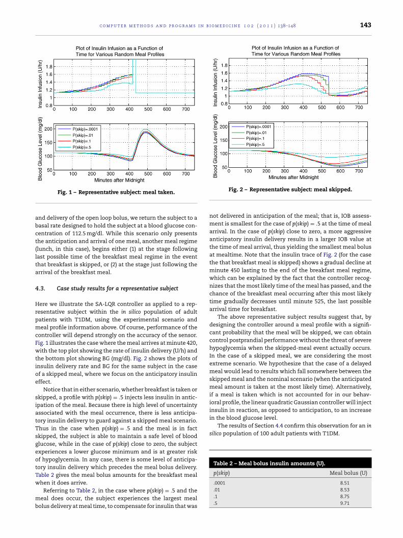

Journal Identification = COMM Article Identification = 3055 Date: April 21, 2011 Time: 9:2 am

c o m p u t e r m e t h o d s a n d p r o g r a m s i n b i o m e d i c i n e 1 0 2 ( 2 0 1 1 ) 138–148 143

abct(lta

4

HrpmcFwtioe

siatTsgeotTw

mb

in the blood glucose level.The results of Section 4.4 confirm this observation for an in

silico population of 100 adult patients with T1DM.

Table 2 – Meal bolus insulin amounts (U).

p(skip) Meal bolus (U)

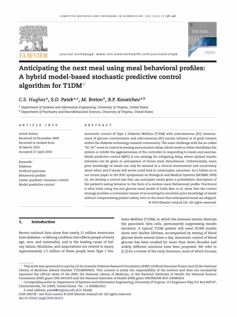
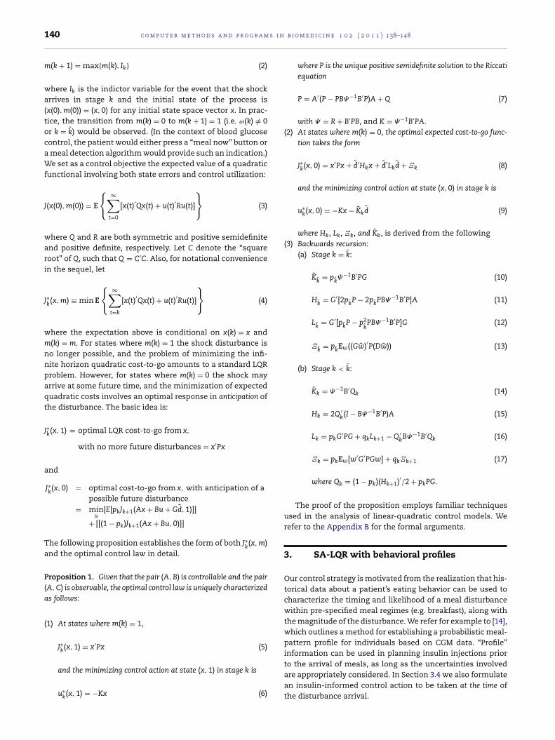
Fig. 1 – Representative subject: meal taken.

nd delivery of the open loop bolus, we return the subject to aasal rate designed to hold the subject at a blood glucose con-entration of 112.5 mg/dl. While this scenario only presentshe anticipation and arrival of one meal, another meal regimelunch, in this case), begins either (1) at the stage followingast possible time of the breakfast meal regime in the eventhat breakfast is skipped, or (2) at the stage just following therrival of the breakfast meal.

.3. Case study results for a representative subject

ere we illustrate the SA-LQR controller as applied to a rep-esentative subject within the in silico population of adultatients with T1DM, using the experimental scenario andeal profile information above. Of course, performance of the

ontroller will depend strongly on the accuracy of the sensor.ig. 1 illustrates the case where the meal arrives at minute 420,ith the top plot showing the rate of insulin delivery (U/h) and

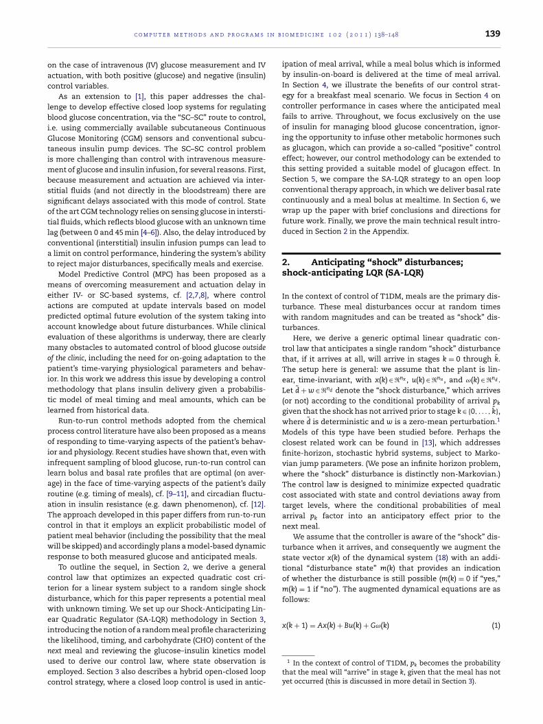
he bottom plot showing BG (mg/dl). Fig. 2 shows the plots ofnsulin delivery rate and BG for the same subject in the casef a skipped meal, where we focus on the anticipatory insulinffect.

Notice that in either scenario, whether breakfast is taken orkipped, a profile with p(skip) = .5 injects less insulin in antic-pation of the meal. Because there is high level of uncertaintyssociated with the meal occurrence, there is less anticipa-ory insulin delivery to guard against a skipped meal scenario.hus in the case when p(skip) = .5 and the meal is in factkipped, the subject is able to maintain a safe level of bloodlucose, while in the case of p(skip) close to zero, the subjectxperiences a lower glucose minimum and is at greater riskf hypoglycemia. In any case, there is some level of anticipa-ory insulin delivery which precedes the meal bolus delivery.able 2 gives the meal bolus amounts for the breakfast meal

hen it does arrive.

Referring to Table 2, in the case where p(skip) = .5 and theeal does occur, the subject experiences the largest meal

olus delivery at meal time, to compensate for insulin that was

Fig. 2 – Representative subject: meal skipped.

not delivered in anticipation of the meal; that is, IOB assess-ment is smallest for the case of p(skip) = .5 at the time of mealarrival. In the case of p(skip) close to zero, a more aggressiveanticipatory insulin delivery results in a larger IOB value atthe time of meal arrival, thus yielding the smallest meal bolusat mealtime. Note that the insulin trace of Fig. 2 (for the casethe that breakfast meal is skipped) shows a gradual decline atminute 450 lasting to the end of the breakfast meal regime,which can be explained by the fact that the controller recog-nizes that the most likely time of the meal has passed, and thechance of the breakfast meal occurring after this most likelytime gradually decreases until minute 525, the last possiblearrival time for breakfast.

The above representative subject results suggest that, bydesigning the controller around a meal profile with a signifi-cant probability that the meal will be skipped, we can obtaincontrol postprandial performance without the threat of severehypoglycemia when the skipped-meal event actually occurs.In the case of a skipped meal, we are considering the mostextreme scenario. We hypothesize that the case of a delayedmeal would lead to results which fall somewhere between theskipped meal and the nominal scenario (when the anticipatedmeal amount is taken at the most likely time). Alternatively,if a meal is taken which is not accounted for in our behav-ioral profile, the linear quadratic Gaussian controller will injectinsulin in reaction, as opposed to anticipation, to an increase

.0001 8.51

.01 8.53

.1 8.75

.5 9.71

Journal Identification = COMM Article Identification = 3055 Date: April 21, 2011 Time: 9:2 am

144 c o m p u t e r m e t h o d s a n d p r o g r a m s i n b i o m e d i c i n e 1 0 2 ( 2 0 1 1 ) 138–148

Table 3 – Results of the population study

Meal skipped meanpre-breakfast min

(std deviation)

Meal taken meanpost-breakfast max

(std deviation)

Noisy CGMp(skip) = .0001 62.22 (10.38) 143.90 (26.75)

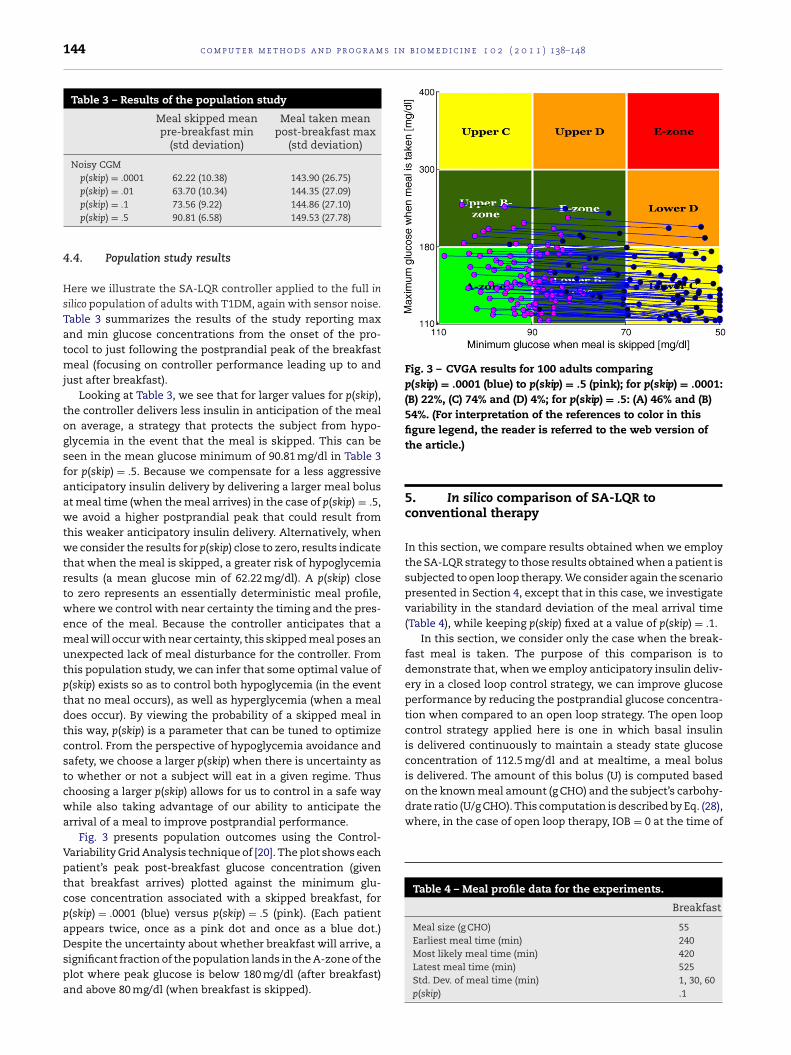
Fig. 3 – CVGA results for 100 adults comparingp(skip) = .0001 (blue) to p(skip) = .5 (pink); for p(skip) = .0001:(B) 22%, (C) 74% and (D) 4%; for p(skip) = .5: (A) 46% and (B)54%. (For interpretation of the references to color in this

is delivered. The amount of this bolus (U) is computed basedon the known meal amount (g CHO) and the subject’s carbohy-drate ratio (U/g CHO). This computation is described by Eq. (28),where, in the case of open loop therapy, IOB = 0 at the time of

Table 4 – Meal profile data for the experiments.

Breakfast

Meal size (g CHO) 55Earliest meal time (min) 240

p(skip) = .01 63.70 (10.34) 144.35 (27.09)p(skip) = .1 73.56 (9.22) 144.86 (27.10)p(skip) = .5 90.81 (6.58) 149.53 (27.78)

4.4. Population study results

Here we illustrate the SA-LQR controller applied to the full insilico population of adults with T1DM, again with sensor noise.Table 3 summarizes the results of the study reporting maxand min glucose concentrations from the onset of the pro-tocol to just following the postprandial peak of the breakfastmeal (focusing on controller performance leading up to andjust after breakfast).

Looking at Table 3, we see that for larger values for p(skip),the controller delivers less insulin in anticipation of the mealon average, a strategy that protects the subject from hypo-glycemia in the event that the meal is skipped. This can beseen in the mean glucose minimum of 90.81 mg/dl in Table 3for p(skip) = .5. Because we compensate for a less aggressiveanticipatory insulin delivery by delivering a larger meal bolusat meal time (when the meal arrives) in the case of p(skip) = .5,we avoid a higher postprandial peak that could result fromthis weaker anticipatory insulin delivery. Alternatively, whenwe consider the results for p(skip) close to zero, results indicatethat when the meal is skipped, a greater risk of hypoglycemiaresults (a mean glucose min of 62.22 mg/dl). A p(skip) closeto zero represents an essentially deterministic meal profile,where we control with near certainty the timing and the pres-ence of the meal. Because the controller anticipates that ameal will occur with near certainty, this skipped meal poses anunexpected lack of meal disturbance for the controller. Fromthis population study, we can infer that some optimal value ofp(skip) exists so as to control both hypoglycemia (in the eventthat no meal occurs), as well as hyperglycemia (when a mealdoes occur). By viewing the probability of a skipped meal inthis way, p(skip) is a parameter that can be tuned to optimizecontrol. From the perspective of hypoglycemia avoidance andsafety, we choose a larger p(skip) when there is uncertainty asto whether or not a subject will eat in a given regime. Thuschoosing a larger p(skip) allows for us to control in a safe waywhile also taking advantage of our ability to anticipate thearrival of a meal to improve postprandial performance.

Fig. 3 presents population outcomes using the Control-Variability Grid Analysis technique of [20]. The plot shows eachpatient’s peak post-breakfast glucose concentration (giventhat breakfast arrives) plotted against the minimum glu-cose concentration associated with a skipped breakfast, forp(skip) = .0001 (blue) versus p(skip) = .5 (pink). (Each patientappears twice, once as a pink dot and once as a blue dot.)Despite the uncertainty about whether breakfast will arrive, a

significant fraction of the population lands in the A-zone of theplot where peak glucose is below 180 mg/dl (after breakfast)and above 80 mg/dl (when breakfast is skipped).

figure legend, the reader is referred to the web version ofthe article.)

5. In silico comparison of SA-LQR toconventional therapy

In this section, we compare results obtained when we employthe SA-LQR strategy to those results obtained when a patient issubjected to open loop therapy. We consider again the scenariopresented in Section 4, except that in this case, we investigatevariability in the standard deviation of the meal arrival time(Table 4), while keeping p(skip) fixed at a value of p(skip) = .1.

In this section, we consider only the case when the break-fast meal is taken. The purpose of this comparison is todemonstrate that, when we employ anticipatory insulin deliv-ery in a closed loop control strategy, we can improve glucoseperformance by reducing the postprandial glucose concentra-tion when compared to an open loop strategy. The open loopcontrol strategy applied here is one in which basal insulinis delivered continuously to maintain a steady state glucoseconcentration of 112.5 mg/dl and at mealtime, a meal bolus

Most likely meal time (min) 420Latest meal time (min) 525Std. Dev. of meal time (min) 1, 30, 60p(skip) .1

Journal Identification = COMM Article Identification = 3055 Date: April 21, 2011 Time: 9:2 am

c o m p u t e r m e t h o d s a n d p r o g r a m s i n b i o m e d i c i n e 1 0 2 ( 2 0 1 1 ) 138–148 145

F�

tb

5

Fl

tamatc8mpc

5

Fmfpma

mfs

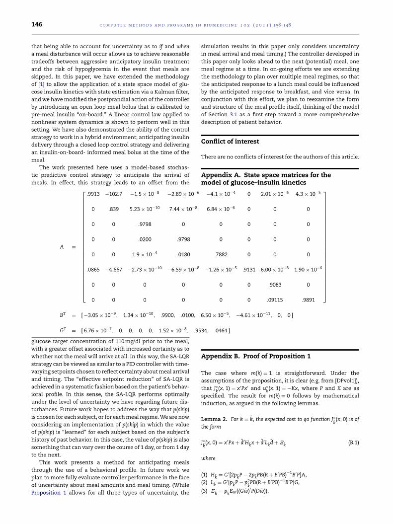
Fig. 5 – CVGA comparing SA-LQR, Std. Dev. 30 min (blue) toopen loop (pink); for SA-LQR: (A) 75% and (B) 25%; for openloop: (A) 88% and (B) 12%. (For interpretation of the

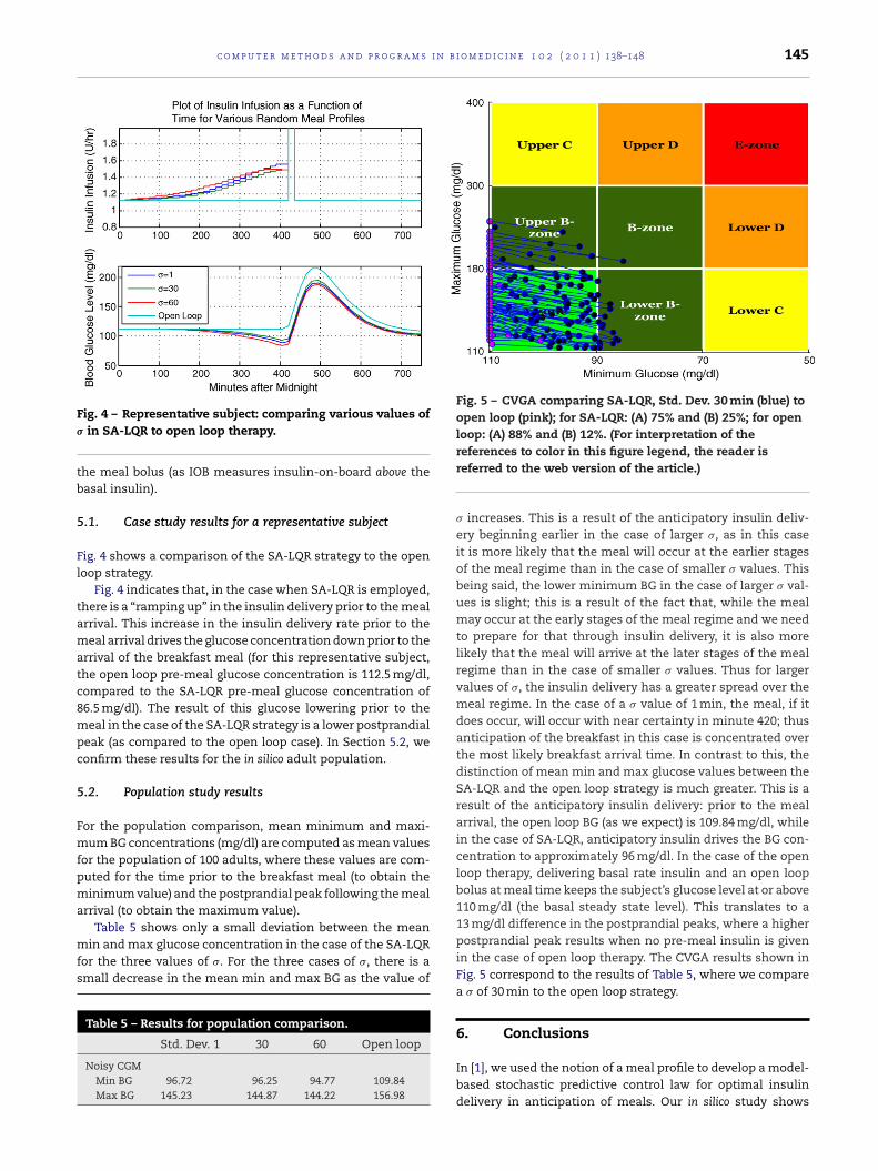
ig. 4 – Representative subject: comparing various values ofin SA-LQR to open loop therapy.

he meal bolus (as IOB measures insulin-on-board above theasal insulin).

.1. Case study results for a representative subject

ig. 4 shows a comparison of the SA-LQR strategy to the openoop strategy.

Fig. 4 indicates that, in the case when SA-LQR is employed,here is a “ramping up” in the insulin delivery prior to the mealrrival. This increase in the insulin delivery rate prior to theeal arrival drives the glucose concentration down prior to the

rrival of the breakfast meal (for this representative subject,he open loop pre-meal glucose concentration is 112.5 mg/dl,ompared to the SA-LQR pre-meal glucose concentration of6.5 mg/dl). The result of this glucose lowering prior to theeal in the case of the SA-LQR strategy is a lower postprandial

eak (as compared to the open loop case). In Section 5.2, weonfirm these results for the in silico adult population.

.2. Population study results

or the population comparison, mean minimum and maxi-um BG concentrations (mg/dl) are computed as mean values

or the population of 100 adults, where these values are com-uted for the time prior to the breakfast meal (to obtain theinimum value) and the postprandial peak following the meal

rrival (to obtain the maximum value).

Table 5 shows only a small deviation between the mean

in and max glucose concentration in the case of the SA-LQRor the three values of �. For the three cases of �, there is amall decrease in the mean min and max BG as the value of

Table 5 – Results for population comparison.

Std. Dev. 1 30 60 Open loop

Noisy CGMMin BG 96.72 96.25 94.77 109.84Max BG 145.23 144.87 144.22 156.98

references to color in this figure legend, the reader isreferred to the web version of the article.)

� increases. This is a result of the anticipatory insulin deliv-ery beginning earlier in the case of larger �, as in this caseit is more likely that the meal will occur at the earlier stagesof the meal regime than in the case of smaller � values. Thisbeing said, the lower minimum BG in the case of larger � val-ues is slight; this is a result of the fact that, while the mealmay occur at the early stages of the meal regime and we needto prepare for that through insulin delivery, it is also morelikely that the meal will arrive at the later stages of the mealregime than in the case of smaller � values. Thus for largervalues of �, the insulin delivery has a greater spread over themeal regime. In the case of a � value of 1 min, the meal, if itdoes occur, will occur with near certainty in minute 420; thusanticipation of the breakfast in this case is concentrated overthe most likely breakfast arrival time. In contrast to this, thedistinction of mean min and max glucose values between theSA-LQR and the open loop strategy is much greater. This is aresult of the anticipatory insulin delivery: prior to the mealarrival, the open loop BG (as we expect) is 109.84 mg/dl, whilein the case of SA-LQR, anticipatory insulin drives the BG con-centration to approximately 96 mg/dl. In the case of the openloop therapy, delivering basal rate insulin and an open loopbolus at meal time keeps the subject’s glucose level at or above110 mg/dl (the basal steady state level). This translates to a13 mg/dl difference in the postprandial peaks, where a higherpostprandial peak results when no pre-meal insulin is givenin the case of open loop therapy. The CVGA results shown inFig. 5 correspond to the results of Table 5, where we comparea � of 30 min to the open loop strategy.

6. Conclusions

In [1], we used the notion of a meal profile to develop a model-based stochastic predictive control law for optimal insulindelivery in anticipation of meals. Our in silico study shows

Journal Identification = COMM Article Identification = 3055 Date: April 21, 2011 Time: 9:2 am

s i n

0−6

0−8

0−8

0,

.95

146 c o m p u t e r m e t h o d s a n d p r o g r a m

that being able to account for uncertainty as to if and whena meal disturbance will occur allows us to achieve reasonabletradeoffs between aggressive anticipatory insulin treatmentand the risk of hypoglycemia in the event that meals areskipped. In this paper, we have extended the methodologyof [1] to allow the application of a state space model of glu-cose insulin kinetics with state estimation via a Kalman filter,and we have modified the postprandial action of the controllerby introducing an open loop meal bolus that is calibrated topre-meal insulin “on-board.” A linear control law applied tononlinear system dynamics is shown to perform well in thissetting. We have also demonstrated the ability of the controlstrategy to work in a hybrid environment; anticipating insulindelivery through a closed loop control strategy and deliveringan insulin-on-board- informed meal bolus at the time of themeal.

The work presented here uses a model-based stochas-tic predictive control strategy to anticipate the arrival ofmeals. In effect, this strategy leads to an offset from the

glucose target concentration of 110 mg/dl prior to the meal,with a greater offset associated with increased certainty as towhether not the meal will arrive at all. In this way, the SA-LQRstrategy can be viewed as similar to a PID controller with time-varying setpoints chosen to reflect certainty about meal arrivaland timing. The “effective setpoint reduction” of SA-LQR isachieved in a systematic fashion based on the patient’s behav-ioral profile. In this sense, the SA-LQR performs optimallyunder the level of uncertainty we have regarding future dis-turbances. Future work hopes to address the way that p(skip)is chosen for each subject, or for each meal regime. We are nowconsidering an implementation of p(skip) in which the valueof p(skip) is “learned” for each subject based on the subject’shistory of past behavior. In this case, the value of p(skip) is alsosomething that can vary over the course of 1 day, or from 1 dayto the next.

This work presents a method for anticipating meals

A =

⎡⎢⎢⎢⎢⎢⎢⎢⎢⎢⎢⎢⎢⎢⎢⎢⎢⎢⎢⎢⎢⎢⎢⎣

.9913 −102.7 −1.5 × 10−8 −2.89 × 1

0 .839 5.23 × 10−10 7.44 × 1

0 0 .9798 0

0 0 .0200 .9798

0 0 1.9 × 10−4 .0180

.0865 −4.667 −2.73 × 10−10 −6.59 × 1

0 0 0 0

0 0 0 0

BT = [ −3.05 × 10−9, 1.34 × 10−10, .9900, .010

GT = [ 6.76 × 10−7, 0, 0, 0, 0, 1.52 × 10−8,

through the use of a behavioral profile. In future work weplan to more fully evaluate controller performance in the faceof uncertainty about meal amounts and meal timing. (WhileProposition 1 allows for all three types of uncertainty, the

b i o m e d i c i n e 1 0 2 ( 2 0 1 1 ) 138–148

simulation results in this paper only considers uncertaintyin meal arrival and meal timing.) The controller developed inthis paper only looks ahead to the next (potential) meal, onemeal regime at a time. In on-going efforts we are extendingthe methodology to plan over multiple meal regimes, so thatthe anticipated response to a lunch meal could be influencedby the anticipated response to breakfast, and vice versa. Inconjunction with this effort, we plan to reexamine the formand structure of the meal profile itself, thinking of the modelof Section 3.1 as a first step toward a more comprehensivedescription of patient behavior.

Conflict of interest

There are no conflicts of interest for the authors of this article.

Appendix A. State space matrices for themodel of glucose–insulin kinetics

−4.1 × 10−4 0 2.01 × 10−6 4.3 × 10−5

6.84 × 10−6 0 0 0

0 0 0 0

0 0 0 0

.7882 0 0 0

−1.26 × 10−5 .9131 6.00 × 10−8 1.90 × 10−6

0 0 .9083 0

0 0 .09115 .9891

⎤⎥⎥⎥⎥⎥⎥⎥⎥⎥⎥⎥⎥⎥⎥⎥⎥⎥⎥⎥⎥⎥⎥⎦

6.50 × 10−5, −4.61 × 10−11, 0, 0 ]

34, .0464 ]

Appendix B. Proof of Proposition 1

The case where m(k) = 1 is straightforward. Under theassumptions of the proposition, it is clear (e.g. from [DPvol1]),that J∗

k(x, 1) = x′Px′ and u∗

k(x, 1) = −Kx, where P and K are as

specified. The result for m(k) = 0 follows by mathematicalinduction, as argued in the following lemmas.

Lemma 2. For k = k̄, the expected cost to go function J∗k̄(x, 0) is of

the form

J∗k̄(x, 0) = x′Px + d̃′H

k̄x + d̃′L

k̄d̃ + �

k̄(B.1)

where

(1) Hk̄

= G′[2pk̄P − 2p

k̄PB(R + B′PB)−1B′P]A,

(2) Lk̄

= G′[pk̄P − p2

k̄PB(R + B′PB)−1B′P]G,

(3) �k̄

= pk̄Ew((Gw̃)′P(Dw̃)),

Journal Identification = COMM Article Identification = 3055 Date: April 21, 2011 Time: 9:2 am

i n b i

a

u

w

P

Tz

u

P

wP

Lo

J

w

kd̃)

x

c o m p u t e r m e t h o d s a n d p r o g r a m s

nd the optimal control action at this state is

∗k̄(x, 0) = −�−1(B′PAx + p

k̄B′PGd̃) (B.2)

here � = R + B′PB.

roof. By straightforward dynamic programming:

J∗k̄(x, 0) = min

u[x′Qx + u′Ru + p

k̄Ew(J∗

k̄+1(Ax + Bu + G(d̃ + w), 1))

+ (1 − pk̄)J∗

k̄+1(Ax + Bu, 1)]

= minu

[x′Qx + u′Ru + pk̄Ew((Ax + Bu + G(d̃ + w))

′

× P(Ax + Bu + G(d̃ + w))) + (1 − pk̄)(Ax + Bu)′

× P(Ax + Bu)]= min

u[x′Qx + u′Ru + (Ax + Bu)′P(Ax + Bu)

+ 2pk̄Ew((G(d̃+w))

′P(Ax+Bu))+p

k̄Ew((G(d̃ + w))

′

× PG(d̃ + w))]= min

u[x′Qx + u′Ru + (Ax + Bu)′P(Ax + Bu)

+ 2pk̄(Gd̃)

′P(Ax + Bu) + p

k̄(Gd̃)

′P(Dd̃)

+ 2pk̄Ew((Gw̃)′P(Dd̃)) + p

k̄Ew((Gw̃)′P(Dw̃))]

= minu

[x′Qx + u′Ru + (Ax)′P(Ax) + 2(Ax)′P(Bu)

+ (Bu)′P(Bu) + 2pk̄(Gd̃)

′P(Ax) + 2p

k̄(Gd̃)

′P(Bu)

+ pk̄(Gd̃)

′P(Dd̃) + �

k̄].

(B.3)

aking the derivative with respect to u and setting equal toero, we get the optimal control

∗k̄(x, 0) = Argmin

u[x′Qx+u′Ru+p

k̄Ew(J∗

k̄+1(Ax + Bu + G(d̃ + w), 1))

+ (1 − pk̄)J∗

k̄+1(Ax + Bu, 1)]

= −(R + B′PB)−1(B′PAx + pk̄B′PGd̃) (B.4)

lugging back into the expression above, we get

J∗k̄(x, 0) = [x′Qx + x′A′PAx + 2p

k̄d̃′G′PAx + p

k̄d̃′G′PGd̃

+ u∗k̄(x, 0)′(R + B′PB)u∗

k̄(x, 0)

+ 2(x′A′PB + pk̄d̃′G′PB)u∗

k̄(x, 0) + �

k̄]

= [x′Qx + x′A′PAx + 2pk̄d̃′G′PAx + p

k̄d̃′G′PGd̃

− (x′A′PB + pk̄d̃′G′PB)(R + B′PB)−1

× (B′PAx + pk̄B′PGd̃) + �

k̄]

= [x′Qx + x′A′PAx − x′A′PB(R + B′PB)−1B′PAx

+ 2pk̄d̃′G′PAx − 2p

k̄d̃′G′PB(R + B′PB)−1B′PAx

+ pk̄d̃′G′PGd̃ − p2

k̄d̃′G′PB(R + B′PB)−1B′PGd̃ + �

k̄]

= [x′[Q + A′[P − PB(R + B′PB)−1B′P]A]x+ d̃′G′[2p

k̄P − 2p

k̄PB(R + B′PB)−1B′P]Ax

+ d̃′G′[pk̄P − p2

k̄PB(R + B′PB)−1B′P]Gd̃ + �

k̄]

= x′Px + d̃′Hk̄x + d̃′L

k̄d̃ + �

k̄,

(B.5)

here we have used the fact that P = Q + A′[P −B(R + B′PB)−1B′P]A. �

emma 3. For k < k̄, the expected cost to go function J∗k(x, 0) is also

f the form:

∗k(x, 0) = x′Px + d̃′Hkx + d̃′Lkd̃ + �k (B.6)

here

o m e d i c i n e 1 0 2 ( 2 0 1 1 ) 138–148 147

(1) Hk = 2Q ′k(I − B�−1B′P)A

(2) Lk = pkG′PG + (1 − pk)Lk+1 − Q ′kB�−1B′Qk (symmetric)

(3) �k = pkEw[w′G′PGw] + (1 − pk)�k+1.

and

(4) Qk = (1 − pk)(Hk+1)′/2 + pkPG.

The optimal policy is

u∗k(x, 0) = −�−1B′[PAx + Qkd̃] (B.7)

Proof. Using the induction hypothesis:

J∗k(x, 0) = min

u[x′Qx + u′Ru + p

k̄Ew(J∗k+1(Ax + Bu + G(d̃ + w), 1))

+ (1 − pk̄)J∗

k+1(Ax + Bu, 0)](B.8)

J∗k(x, 0) = min

u[x′Qx + u′Ru + p

k̄Ew[(Ax + Bu + G(d̃ + w))

′

× P(Ax + Bu + G(d̃ + w))] + (1 − pk̄)

× [(Ax + Bu)′P(Ax + Bu) + d̃′Hk+1(Ax + Bu) + d̃′Lk+1d̃

+ �k+1]]= min

u[x′Qx + u′Ru + p

k̄[(Ax + Bu)′P(Ax + Bu)

+ 2Ew((G(d̃ + w))′P(Ax + Bu))

+ Ew((G(d̃ + w))′PG(d̃ + w))]

+ (1 − pk̄)[(Ax + Bu)′P(Ax + Bu) + d̃′Hk+1(Ax + Bu)

+ d̃′Lk+1d̃ + �k+1]]= min

u[x′Qx + u′Ru + (Ax + Bu)′P(Ax + Bu)

+ pk̄[2(Gd̃)

′P(Ax + Bu) + (Gd̃)

′PGd̃ + Ew((Gw)′PGw)]

+ (1 − pk̄)[d̃′Hk+1(Ax + Bu) + d̃′Lk+1d̃ + �k+1]]

= minu

[x′Qx + u′Ru + (Ax + Bu)′P(Ax + Bu)

+ pk̄[2(Gd̃)

′P(Ax + Bu) + (Gd̃)

′PGd̃]

+ (1 − pk̄)[d̃′Hk+1(Ax + Bu) + d̃′Lk+1d̃] + �k]

= minu

[x′(Q + A′PA)x + u′�u + [2x′A′P + 2d̃′Q ′k]Bu

+ 2d̃′Q ′kAx + d̃′[pkG′PG + (1 − pk)Lk+1]d̃′ + �k]

(B.9)

Taking the derivative with respect to u and setting equal tozero, we get

2�u + 2B′[PAx + Qkd̃] = 0

so that u∗k(x, 0) = −�−1B′[PAx + Qkd̃]. Plugging into the expres-

sion above, we get

J∗k(x, 0) = [x′(Q + A′PA)x + (x′A′P + d̃′Q ′

k)B�−1��−1B′(PAx + Q

− (2x′A′P + 2d̃′Q ′k)B�−1B′(PAx + Qkd̃) + 2d̃′Q ′

kAx

+ d̃′(pkG′PG + (1 − pk)Lk+1)d̃ + �k]= [x′(Q + A′PA)x − (x′A′P + d̃′Q ′

k)B�−1B′(PAx + Qkd̃)

+ 2d̃′Q ′kAx + d̃′(pkG′PG + (1 − pk)Lk+1)d̃ + �k]

= [x′(Q + A′PA)x − x′A′PB�−1B′PAx + 2d̃′Q ′kAx

− 2x′A′PB�−1B′Qkd̃ + d̃′(pkG′PG + (1 − pk)Lk+1)d̃− d̃′Q ′

kB�−1B′Qkd̃ + �k]

= [x′[Q + A′(P − PB�−1B′P)A]x + d̃′[2Q ′k(I − B�−1B′P)A]

+ d̃′[pkG′PG + (1 − pk)Lk+1 − Q ′ B�−1B′Qk]d̃ + �k]

(B.10)

k

= x′Px + d̃′Hkx + d̃′Lkd̃ + �k

where again we have used the fact that P = Q + A′[P −PB(R + B′PB)−1B′P]A. �

Journal Identification = COMM Article Identification = 3055 Date: April 21, 2011 Time: 9:2 am

s i n

r

[20] L. Magni, D.M. Raimondo, C. Dalla Man, M. Breton, S.D.

148 c o m p u t e r m e t h o d s a n d p r o g r a m

e f e r e n c e s

[1] S. Patek, C. Hughes, M. Breton, B. Kovatchev, Anticipatingmeals with behavioral profiles: towards stochastic modelpredictive control of T1DM, in: Proceedings of the 7th IFACSymposium on Modelling and Control in BiomedicalSystems, 2009, pp. 37–42, Available in IFAC Papers-OnLine:http://www.ifac-papersonline.net/Detailed/39984.html.

[2] R.S. Parker, F.J. Doyle, N.A. Peppas III, A model-basedalgorithm for blood glucose control in type 1 diabeticpatients, IEEE Trans. Biomed. Eng. BME-46 (2) (1999)148–157.

[3] B.W. Bequette, A critical assessment of algorithms andchallenges in the development of a closed-loop artificialpancreas, Diab. Technol. Ther. 7 (2005) 28–47.

[4] M. Boyne, D.M. Silver, J. Kaplan, C. Saudek, Timing ofchanges in interstitial and venous blood glucose measuredwith a continuous subcutaneous glucose sensor, Diabetes 52(2003) 2790–2794.

[5] K. Rebrin, G. Steil, W. van Antwerp, J. Mastrototaro,Subcutaneous glucose predicts plasma glucose independentof insulin: implications for continuous monitoring, Am. J.Physiol. Endocrinol. Metab. 277 (1999) 561–571.

[6] E. Kulcu, J. Tamada, G. Reach, R. Potts, M. Lesho,Physiological differences between interstitial glucose andblood glucose measured in human subjects, Diabetes Care26 (2003) 2405–2409.

[7] R. Hovorka, V. Canonico, L.J. Chassin, U. Haueter, M.Massi-Benedetti, M.O. Federici, T. Pieber, H. Schaller, L.Schaupp, T. Vering, M.E. Wilinska, Nonlinear modelpredictive control of glucose concentration in subjects withtype 1 diabetes, Physiol. Meas. 25 (2004) 905–920.

[8] L. Magni, D.M. Raimondo, C. Dalla Man, G.D. Nicolao, B.Kovatchev, C. Cobelli, Model predictive control of glucoseconcentration in subjects with type 1 diabetes: an in silico

trial, in: 17th IFAC World Congress, 2008,pp. 4246–4251.

[9] H. Zisser, L. Jovanovic, F.J. Doyle, P. Ospina, C. Owens III,Run-to-run control of meal-related insulin dosing, Diab.Technol. Ther. 7 (2005) 48–57.

b i o m e d i c i n e 1 0 2 ( 2 0 1 1 ) 138–148

[10] C. Owens, H. Zisser, L. Jovanovic, B. Srinivasan, D. Bonvin, F.J.Doyle III, Run-to-run control of blood glucose concentrationsfor people with type 1 diabetes mellitus, IEEE Trans. Biomed.Eng. 53 (2006) 996–1005.

[11] C. Palerm, H. Zisser, W. Bevier, L. Jovanovic, F.J. Doyle III,Prandial insulin dosing using run-to-run control: applicationof clinical data and medical expertise to define a suitableperformance metric, Diabetes Care 30 (2007) 1131–1136.

[12] C. Palerm, H. Zisser, L. Jovanovic, F.J. Doyle III, A run-to-runcontrol strategy to adjust basal insulin infusion rates in type1 diabetes, J. Process Control 18 (2008) 258–265.

[13] L. Campo, Y. Bar-Shalom, Control of discrete-time hybridstochastic systems, IEEE Trans. Autom. Control 37 (10) (1992)1522–1527.

[14] S. Patek, M. Breton, C. Cobelli, C. Dalla Man, B. Kovatchev,Adaptive meal detection algorithm enabling closed-loopcontrol in type 1 diabetes, in: Proceedings of the 2007Diabetes Technology Meeting (Abstract), 2007.

[15] R. Bergman, Y. Ider, C. Bowden, C. Cobelli, Quantitativeestimation of insulin sensitivity, Am. J. Physiol. 236 (1979)E667–E677.

[16] K.L. Swan, J.D. Dziura, G.M. Steil, G.R. Voskanyan, K.A. Sikes,A.T. Steffen, M.L. Martin, W.V. Tamborlane, S.A. Weinzimer,Effect of age of infusion site and type of rapid-acting analogon pharmacodynamic parameters of insulin boluses inyouth with type 1 diabetes receiving insulin pump therapy,Diabetes Care 32 (2009) 240–244.

[17] C. Dalla Man, R.A. Rizza, C. Cobelli, Meal simulation modelof the glucose–insulin system, IEEE Trans. Biomed. Eng. 54(10) (2007) 1740–1749.

[18] C. Dalla Man, D.M. Raimondo, R.A. Rizza, C. Cobelli, GIM,simulation software of meal glucose–insulin model, J.Diabetes Sci. Technol. 1 (3) (2007) 323–330.

[19] M. Breton, B. Kovatchev, Analysis, modeling, and simulationof the accuracy of continuous glucose sensors, J. DiabetesSci. Technol. 2 (5) (2008) 1–10.

Patek, G.D. Nicolao, C. Cobelli, B.P. Kovatchev, Evaluating theefficacy of closed-loop glucose regulation viacontrol-variability grid analysis, J. Diabetes Sci. Technol. 2 (4)(2008) 630–635.