Embed Size (px)
Citation preview
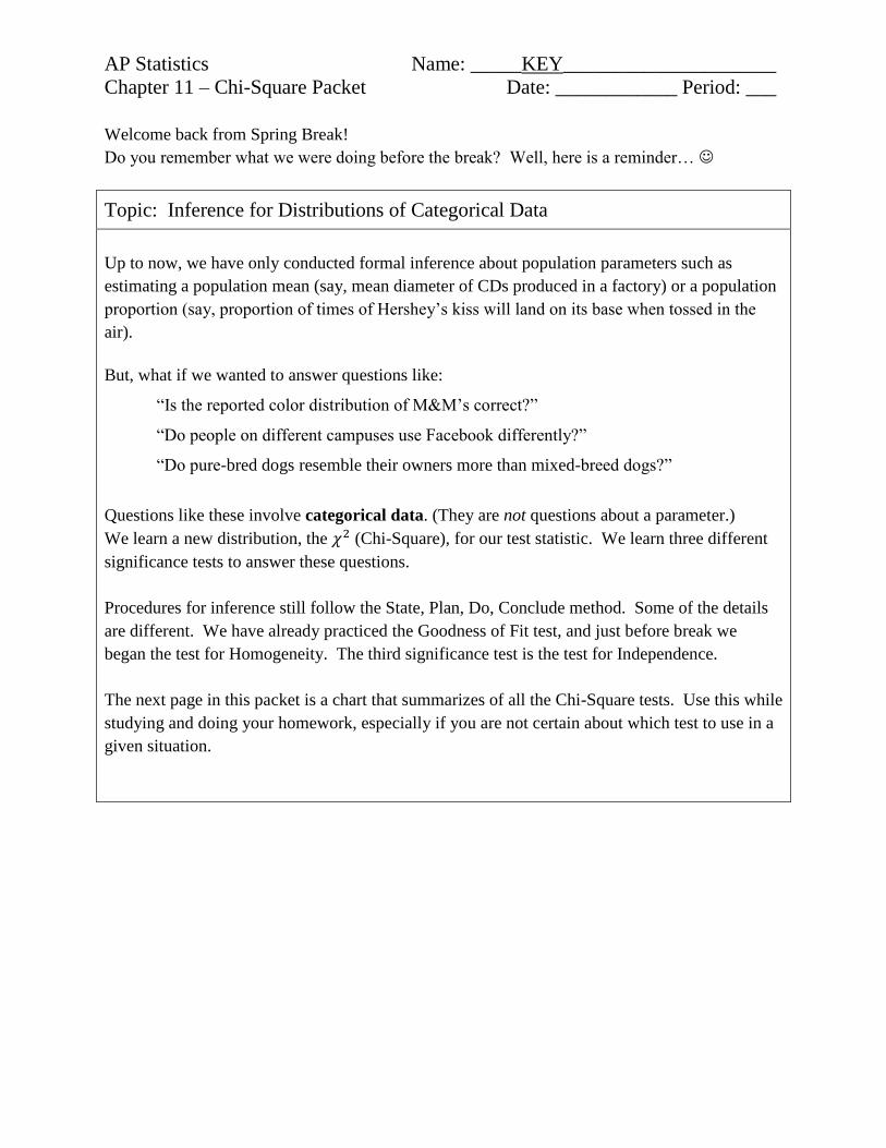
AP Statistics Name: _____KEY_____________________
Chapter 11 – Chi-Square Packet Date: ____________ Period: ___
Welcome back from Spring Break!
Do you remember what we were doing before the break? Well, here is a reminder…
Topic: Inference for Distributions of Categorical Data
Up to now, we have only conducted formal inference about population parameters such as
estimating a population mean (say, mean diameter of CDs produced in a factory) or a population
proportion (say, proportion of times of Hershey’s kiss will land on its base when tossed in the
air).
But, what if we wanted to answer questions like:
“Is the reported color distribution of M&M’s correct?”
“Do people on different campuses use Facebook differently?”
“Do pure-bred dogs resemble their owners more than mixed-breed dogs?”
Questions like these involve categorical data. (They are not questions about a parameter.)
We learn a new distribution, the (Chi-Square), for our test statistic. We learn three different
significance tests to answer these questions.
Procedures for inference still follow the State, Plan, Do, Conclude method. Some of the details
are different. We have already practiced the Goodness of Fit test, and just before break we
began the test for Homogeneity. The third significance test is the test for Independence.
The next page in this packet is a chart that summarizes of all the Chi-Square tests. Use this while
studying and doing your homework, especially if you are not certain about which test to use in a
given situation.
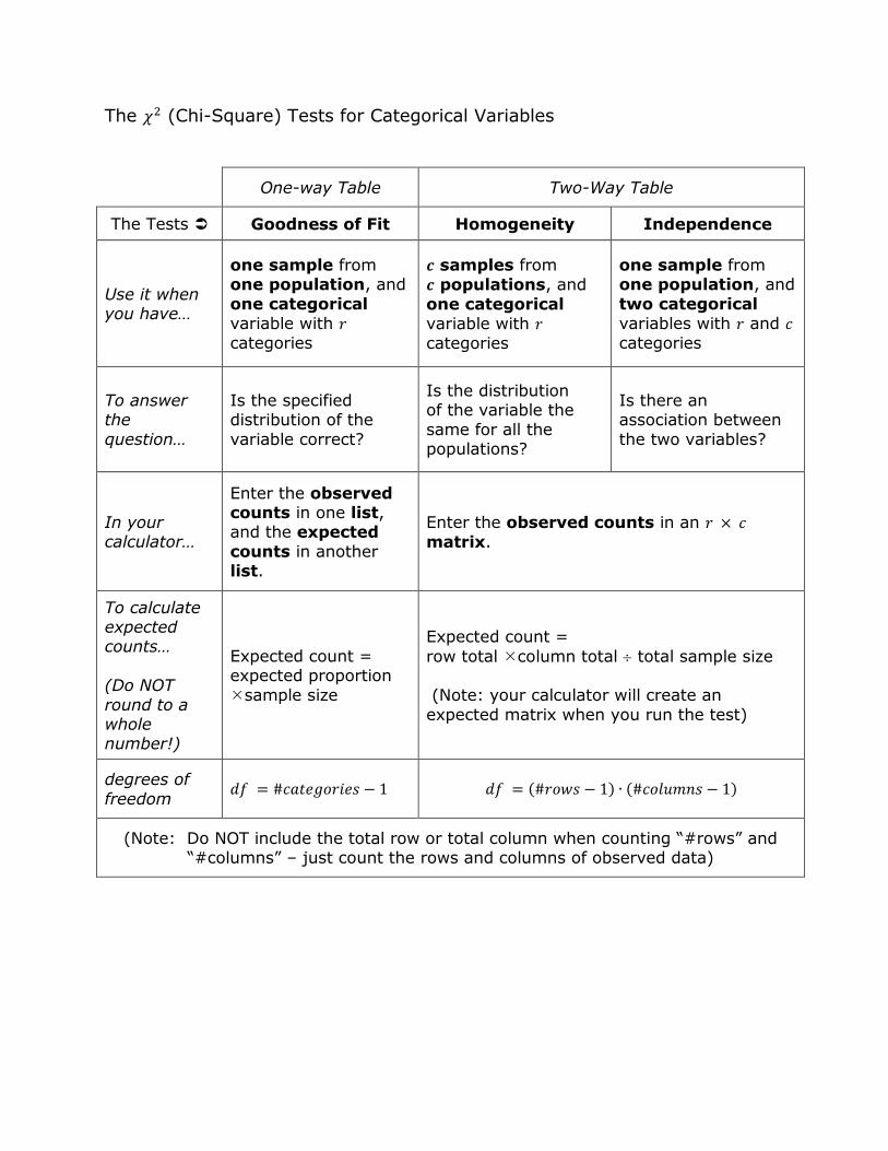
The (Chi-Square) Tests for Categorical Variables
One-way Table Two-Way Table
The Tests Goodness of Fit Homogeneity Independence
Use it when you have…
one sample from one population, and
one categorical
variable with categories
samples from
populations, and
one categorical
variable with categories
one sample from one population, and
two categorical
variables with and categories
To answer the
question…
Is the specified distribution of the
variable correct?
Is the distribution of the variable the
same for all the populations?
Is there an association between
the two variables?
In your calculator…
Enter the observed counts in one list, and the expected
counts in another list.
Enter the observed counts in an matrix.
To calculate expected counts…
(Do NOT
round to a whole number!)
Expected count = expected proportion
sample size
Expected count =
row total column total total sample size (Note: your calculator will create an
expected matrix when you run the test)
degrees of
freedom ( ) ( )
(Note: Do NOT include the total row or total column when counting “#rows” and “#columns” – just count the rows and columns of observed data)
The (Chi-Square) Distributions and the Test Statistic
Shape
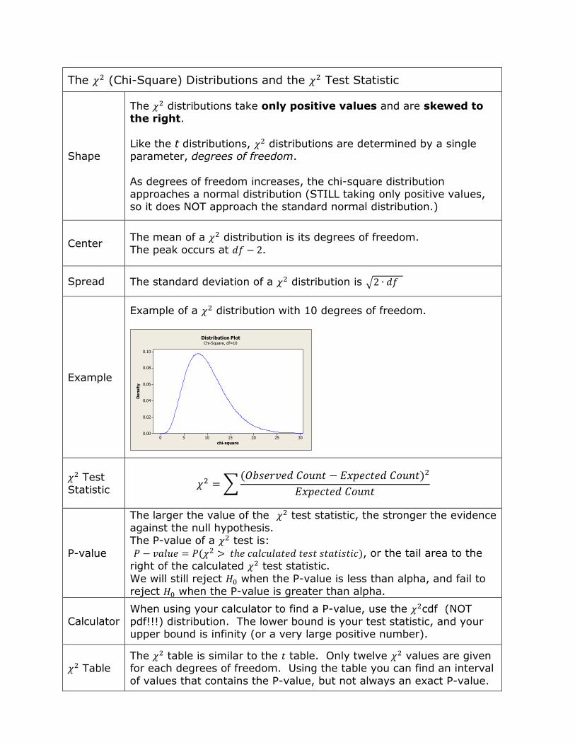
The distributions take only positive values and are skewed to the right.
Like the t distributions, distributions are determined by a single parameter, degrees of freedom.
As degrees of freedom increases, the chi-square distribution
approaches a normal distribution (STILL taking only positive values, so it does NOT approach the standard normal distribution.)
Center The mean of a distribution is its degrees of freedom.
The peak occurs at .
Spread The standard deviation of a distribution is √
Example
Example of a distribution with 10 degrees of freedom.
302520151050
0.10
0.08
0.06
0.04
0.02
0.00
chi-square
De
nsit
y
Distribution PlotChi-Square, df=10
Test
Statistic ∑
( )
P-value
The larger the value of the test statistic, the stronger the evidence
against the null hypothesis.
The P-value of a test is:
( ), or the tail area to the
right of the calculated test statistic.
We will still reject when the P-value is less than alpha, and fail to
reject when the P-value is greater than alpha.
Calculator When using your calculator to find a P-value, use the cdf (NOT
pdf!!!) distribution. The lower bound is your test statistic, and your upper bound is infinity (or a very large positive number).
Table The table is similar to the table. Only twelve values are given for each degrees of freedom. Using the table you can find an interval
of values that contains the P-value, but not always an exact P-value.
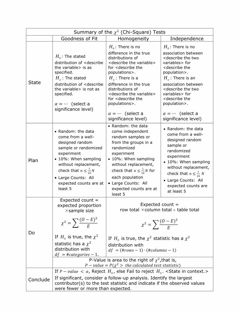
Summary of the (Chi-Square) Tests
Goodness of Fit Homogeneity Independence
State
0H : The stated
distribution of <describe
the variable> is as
specified.
aH : The stated
distribution of <describe
the variable> is not as
specified.
(select a
significance level)
0H : There is no
difference in the true
distributions of
<describe the variable>
for <describe the
populations>.
aH : There is a
difference in the true
distributions of
<describe the variable>
for <describe the
populations>.
(select a
significance level)
0H : There is no
association between
<describe the two
variables> for
<describe the
population>.
aH : There is an
association between
<describe the two
variables> for
<describe the
population>.
(select a
significance level)
Plan
Random: the data
come from a well-
designed random
sample or randomized
experiment
10%: When sampling
without replacement,
check that
Large Counts: All
expected counts are at
least 5
Random: the data
come independent
random samples or
from the groups in a
randomized
experiment
10%: When sampling
without replacement,
check that
for
each population
Large Counts: All
expected counts are at
least 5
Random: the data
come from a well-
designed random
sample or
randomized
experiment
10%: When sampling
without replacement,
check that
Large Counts: All
expected counts are
at least 5
Do
Expected count =
expected proportion sample size
∑( )
If 0H is true, the
statistic has a distribution with .
Expected count =
row total column total table total
∑( )
If 0H is true, the statistic has a
distribution with ( ) ( )
P-Value is area to the right of ,that is, ( )
Conclude
If , Reject 0H , else Fail to reject 0H . <State in context.>
If significant, consider a follow-up analysis. Identify the largest
contributor(s) to the test statistic and indicate if the observed values were fewer or more than expected.
Check Your Understanding: Goodness of Fit
1. What is a one-way table?
A: A table that presents data for one categorical variable.
2. Should you round expected counts to the nearest integer? Explain.
A: No! While observed counts are integer values only, the expected counts can be decimal
because they represent the average number in repeated sampling, for the assumed
distribution.
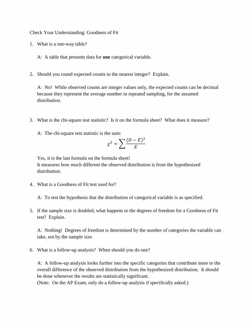
3. What is the chi-square test statistic? Is it on the formula sheet? What does it measure?
A: The chi-square test statistic is the sum:
∑( )
Yes, it is the last formula on the formula sheet!
It measures how much different the observed distribution is from the hypothesized
distribution.
4. What is a Goodness of Fit test used for?
A: To test the hypothesis that the distribution of categorical variable is as specified.
5. If the sample size is doubled, what happens to the degrees of freedom for a Goodness of Fit
test? Explain.
A: Nothing! Degrees of freedom is determined by the number of categories the variable can
take, not by the sample size.
6. What is a follow-up analysis? When should you do one?
A: A follow-up analysis looks further into the specific categories that contribute more to the
overall difference of the observed distribution from the hypothesized distribution. It should
be done whenever the results are statistically significant.
(Note: On the AP Exam, only do a follow-up analysis if specifically asked.)
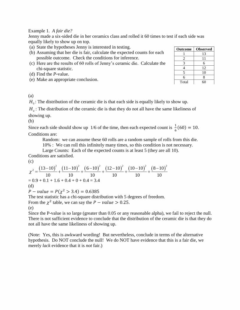
Example 1. A fair die?
Jenny made a six-sided die in her ceramics class and rolled it 60 times to test if each side was
equally likely to show up on top.
(a) State the hypotheses Jenny is interested in testing.
(b) Assuming that her die is fair, calculate the expected counts for each
possible outcome. Check the conditions for inference.
(c) Here are the results of 60 rolls of Jenny’s ceramic die. Calculate the
chi-square statistic.
(d) Find the P-value.
(e) Make an appropriate conclusion.
(a)
0H : The distribution of the ceramic die is that each side is equally likely to show up.
aH : The distribution of the ceramic die is that they do not all have the same likeliness of
showing up.
(b)
Since each side should show up 1/6 of the time, then each expected count is
( ) .
Conditions are:
Random: we can assume these 60 rolls are a random sample of rolls from this die.
10% : We can roll this infinitely many times, so this condition is not necessary.
Large Counts: Each of the expected counts is at least 5 (they are all 10).
Conditions are satisfied.
(c)
2 2 2 2 2 2
2 13 10 11 10 6 10 12 10 10 10 8 10
10 10 10 10 10 10
= 0.9 + 0.1 + 1.6 + 0.4 + 0 + 0.4 = 3.4
(d)
( ) The test statistic has a chi-square distribution with 5 degrees of freedom.
From the table, we can say the .
(e)
Since the P-value is so large (greater than 0.05 or any reasonable alpha), we fail to reject the null.
There is not sufficient evidence to conclude that the distribution of the ceramic die is that they do
not all have the same likeliness of showing up.
(Note: Yes, this is awkward wording! But nevertheless, conclude in terms of the alternative
hypothesis. Do NOT conclude the null! We do NOT have evidence that this is a fair die, we
merely lack evidence that it is not fair.)
Outcome Observed
1 13
2 11
3 6
4 12
5 10
6 8
Total 60
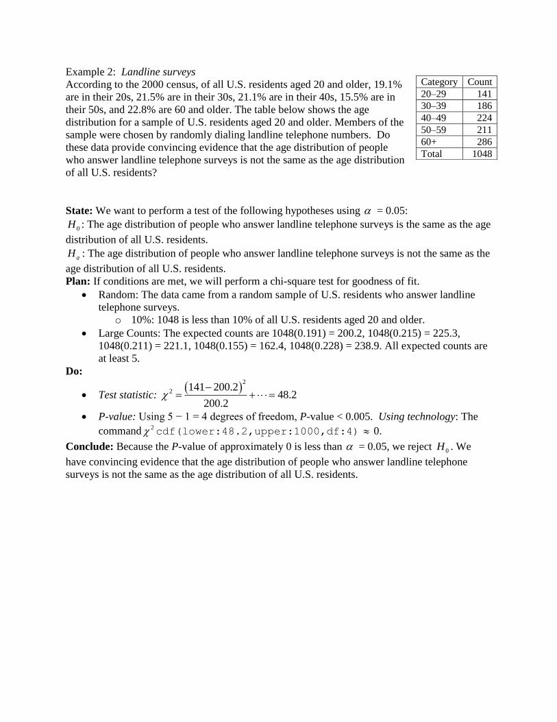
Example 2: Landline surveys
According to the 2000 census, of all U.S. residents aged 20 and older, 19.1%
are in their 20s, 21.5% are in their 30s, 21.1% are in their 40s, 15.5% are in
their 50s, and 22.8% are 60 and older. The table below shows the age
distribution for a sample of U.S. residents aged 20 and older. Members of the
sample were chosen by randomly dialing landline telephone numbers. Do
these data provide convincing evidence that the age distribution of people
who answer landline telephone surveys is not the same as the age distribution
of all U.S. residents?
State: We want to perform a test of the following hypotheses using = 0.05:
0H : The age distribution of people who answer landline telephone surveys is the same as the age
distribution of all U.S. residents.
aH : The age distribution of people who answer landline telephone surveys is not the same as the
age distribution of all U.S. residents.
Plan: If conditions are met, we will perform a chi-square test for goodness of fit.
Random: The data came from a random sample of U.S. residents who answer landline
telephone surveys.
o 10%: 1048 is less than 10% of all U.S. residents aged 20 and older.
Large Counts: The expected counts are 1048(0.191) = 200.2, 1048(0.215) = 225.3,
1048(0.211) = 221.1, 1048(0.155) = 162.4, 1048(0.228) = 238.9. All expected counts are
at least 5.
Do:
Test statistic:
2
2 141 200.248.2
200.2
P-value: Using 5 − 1 = 4 degrees of freedom, P-value < 0.005. Using technology: The
command 2 cdf(lower:48.2,upper:1000,df:4) 0.
Conclude: Because the P-value of approximately 0 is less than = 0.05, we reject 0H . We
have convincing evidence that the age distribution of people who answer landline telephone
surveys is not the same as the age distribution of all U.S. residents.
Category Count
20–29 141
30–39 186
40–49 224
50–59 211
60+ 286
Total 1048
Check Your Understanding: Test for Homogeneity
1. What is a two-way table?
A: A table that presents data for two categorical variables.
2. How do you state hypotheses for a test of homogeneity?
0H : There is no difference in the true distributions of <describe the variable> for <describe the
populations>.
aH : There is a difference in the true distributions of <describe the variable> for <describe the
populations>.
3. What is the problem of multiple comparisons? What strategy should we use to deal with it?
A: When we do many individual tests or construct many confidence intervals, the individual
P-values and confidence levels don’t tell us how confident we can be in all the inferences
taken together. Because of this, it’s cheating to pick out one large difference from the two-
way table and then perform a significance test as if it were the only comparison we had in
mind.
We do one overall test and then a follow-up analysis if the results are significant.
4. What are the conditions for a test for homogeneity?
A:
Random: the data come independent random samples or from the groups in a randomized
experiment
10%: When sampling without replacement, check that n≤1/10 N
Large Counts: All expected counts are at least 5
5. How do you input the data into your calculator for a test for homogeneity?
A: As a matrix! Input the rows and columns of observed counts only. No totals.
6. How do you calculate the expected counts for a test that compares the distribution of a
categorical variable in multiple groups or populations?
A: Row total column total table total
7. How do you calculate the degrees of freedom for a chi-square test for homogeneity?
A: ( ) ( )
0.0000
0.0500
0.1000
0.1500
0.2000
0.2500
Sunday Tuesday Thursday Saturday
Pro
po
rtio
n o
f eac
h a
ge
gro
up
Day of week
Before 1980
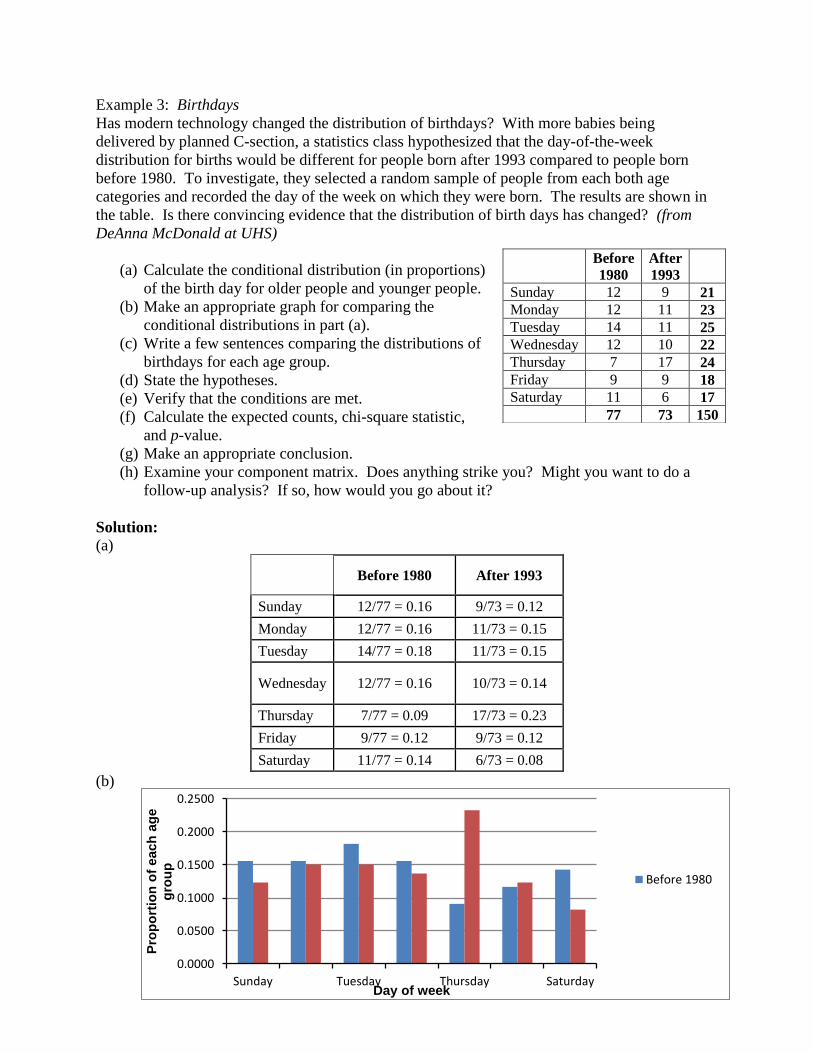
Example 3: Birthdays
Has modern technology changed the distribution of birthdays? With more babies being
delivered by planned C-section, a statistics class hypothesized that the day-of-the-week
distribution for births would be different for people born after 1993 compared to people born
before 1980. To investigate, they selected a random sample of people from each both age
categories and recorded the day of the week on which they were born. The results are shown in
the table. Is there convincing evidence that the distribution of birth days has changed? (from
DeAnna McDonald at UHS)
(a) Calculate the conditional distribution (in proportions)
of the birth day for older people and younger people.
(b) Make an appropriate graph for comparing the
conditional distributions in part (a).
(c) Write a few sentences comparing the distributions of
birthdays for each age group.
(d) State the hypotheses.
(e) Verify that the conditions are met.
(f) Calculate the expected counts, chi-square statistic,
and p-value.
(g) Make an appropriate conclusion.
(h) Examine your component matrix. Does anything strike you? Might you want to do a
follow-up analysis? If so, how would you go about it?
Solution: (a)
Before 1980 After 1993
Sunday 12/77 = 0.16 9/73 = 0.12
Monday 12/77 = 0.16 11/73 = 0.15
Tuesday 14/77 = 0.18 11/73 = 0.15
Wednesday 12/77 = 0.16 10/73 = 0.14
Thursday 7/77 = 0.09 17/73 = 0.23
Friday 9/77 = 0.12 9/73 = 0.12
Saturday 11/77 = 0.14 6/73 = 0.08
(b)
Before
1980
After
1993
Sunday 12 9 21
Monday 12 11 23
Tuesday 14 11 25
Wednesday 12 10 22
Thursday 7 17 24
Friday 9 9 18
Saturday 11 6 17
77 73 150
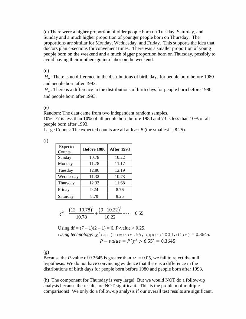
(c) There were a higher proportion of older people born on Tuesday, Saturday, and
Sunday and a much higher proportion of younger people born on Thursday. The
proportions are similar for Monday, Wednesday, and Friday. This supports the idea that
doctors plan c-sections for convenient times. There was a smaller proportion of young
people born on the weekend and a much bigger proportion born on Thursday, possibly to
avoid having their mothers go into labor on the weekend.
(d)
0H : There is no difference in the distributions of birth days for people born before 1980
and people born after 1993.
aH : There is a difference in the distributions of birth days for people born before 1980
and people born after 1993.
(e)
Random: The data came from two independent random samples.
10%: 77 is less than 10% of all people born before 1980 and 73 is less than 10% of all
people born after 1993.
Large Counts: The expected counts are all at least 5 (the smallest is 8.25).
(f)
Expected
Counts Before 1980 After 1993
Sunday 10.78 10.22
Monday 11.78 11.17
Tuesday 12.86 12.19
Wednesday 11.32 10.73
Thursday 12.32 11.68
Friday 9.24 8.76
Saturday 8.70 8.25
2 2
2 12 10.78 9 10.22
10.78 10.22
6.55
Using df = (7 – 1)(2 – 1) = 6, P-value > 0.25.
Using technology: 2 cdf(lower:6.55,upper:1000,df:6) = 0.3645.
( )
(g)
Because the P-value of 0.3645 is greater than = 0.05, we fail to reject the null
hypothesis. We do not have convincing evidence that there is a difference in the
distributions of birth days for people born before 1980 and people born after 1993.
(h) The component for Thursday is very large! But we would NOT do a follow-up
analysis because the results are NOT significant. This is the problem of multiple
comparisons! We only do a follow-up analysis if our overall test results are significant.
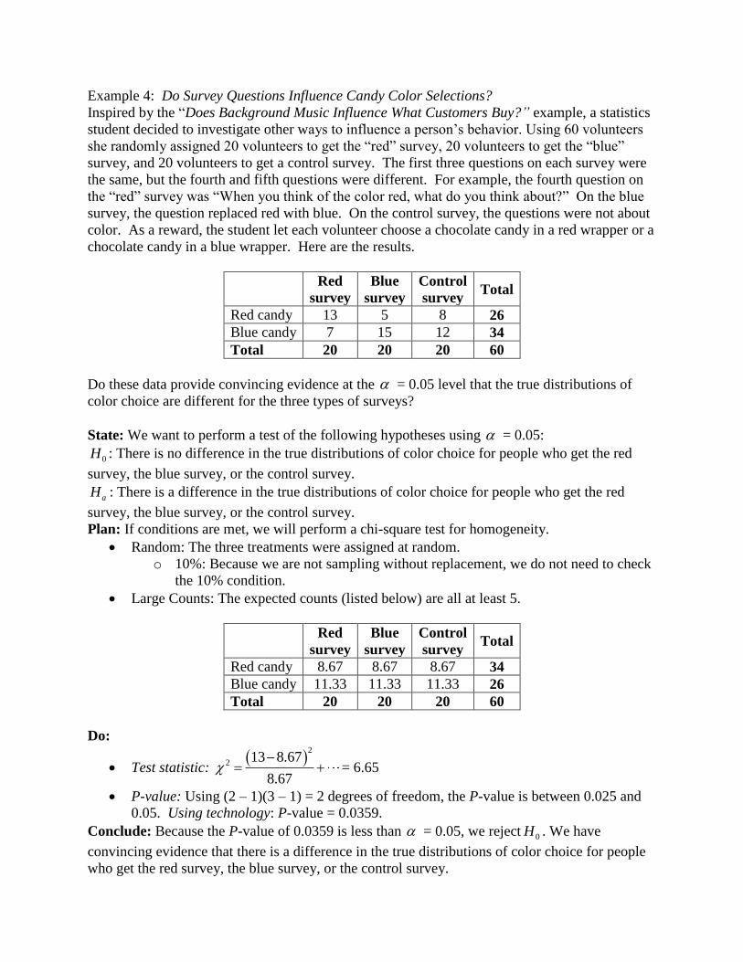
Example 4: Do Survey Questions Influence Candy Color Selections?
Inspired by the “Does Background Music Influence What Customers Buy?” example, a statistics
student decided to investigate other ways to influence a person’s behavior. Using 60 volunteers
she randomly assigned 20 volunteers to get the “red” survey, 20 volunteers to get the “blue”
survey, and 20 volunteers to get a control survey. The first three questions on each survey were
the same, but the fourth and fifth questions were different. For example, the fourth question on
the “red” survey was “When you think of the color red, what do you think about?” On the blue
survey, the question replaced red with blue. On the control survey, the questions were not about
color. As a reward, the student let each volunteer choose a chocolate candy in a red wrapper or a
chocolate candy in a blue wrapper. Here are the results.
Red
survey
Blue
survey
Control
survey Total
Red candy 13 5 8 26
Blue candy 7 15 12 34
Total 20 20 20 60
Do these data provide convincing evidence at the = 0.05 level that the true distributions of
color choice are different for the three types of surveys?
State: We want to perform a test of the following hypotheses using = 0.05:
0H : There is no difference in the true distributions of color choice for people who get the red
survey, the blue survey, or the control survey.
aH : There is a difference in the true distributions of color choice for people who get the red
survey, the blue survey, or the control survey.
Plan: If conditions are met, we will perform a chi-square test for homogeneity.
Random: The three treatments were assigned at random.
o 10%: Because we are not sampling without replacement, we do not need to check
the 10% condition.
Large Counts: The expected counts (listed below) are all at least 5.
Red
survey
Blue
survey
Control
survey Total
Red candy 8.67 8.67 8.67 34
Blue candy 11.33 11.33 11.33 26
Total 20 20 20 60
Do:
Test statistic:
2
2 13 8.67
8.67
= 6.65
P-value: Using (2 – 1)(3 – 1) = 2 degrees of freedom, the P-value is between 0.025 and
0.05. Using technology: P-value = 0.0359.
Conclude: Because the P-value of 0.0359 is less than = 0.05, we reject 0H . We have
convincing evidence that there is a difference in the true distributions of color choice for people
who get the red survey, the blue survey, or the control survey.
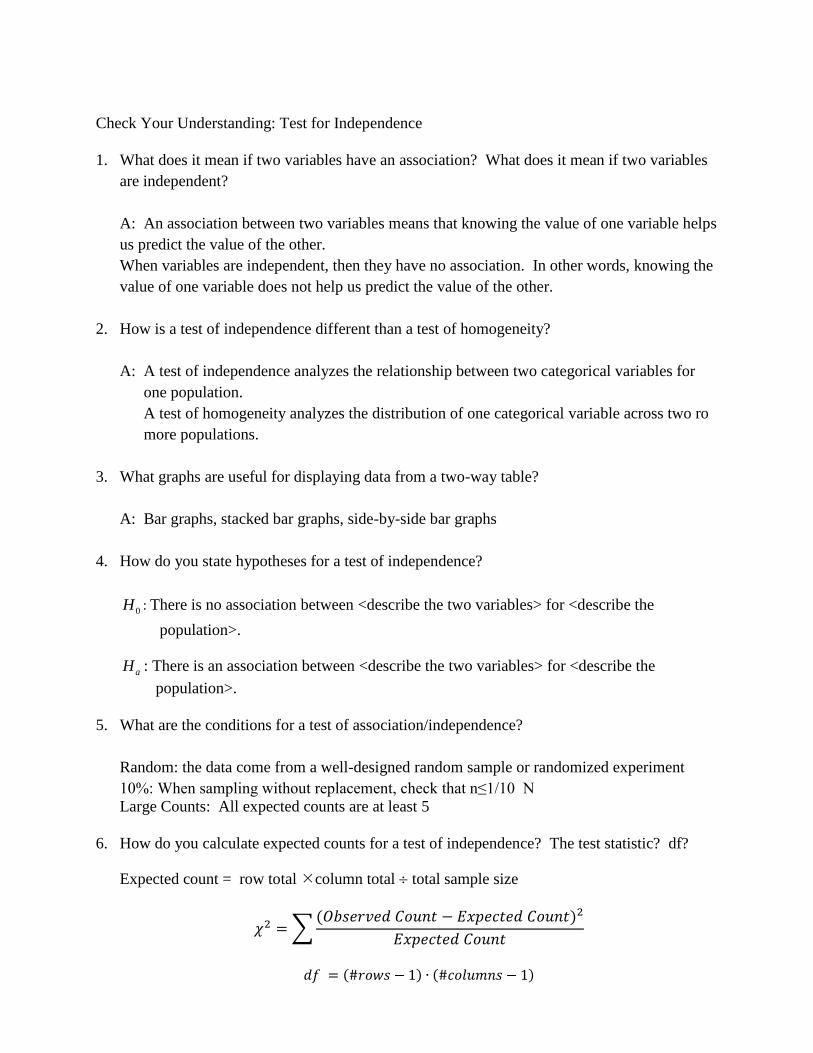
Check Your Understanding: Test for Independence
1. What does it mean if two variables have an association? What does it mean if two variables
are independent?
A: An association between two variables means that knowing the value of one variable helps
us predict the value of the other.
When variables are independent, then they have no association. In other words, knowing the
value of one variable does not help us predict the value of the other.
2. How is a test of independence different than a test of homogeneity?
A: A test of independence analyzes the relationship between two categorical variables for
one population.
A test of homogeneity analyzes the distribution of one categorical variable across two ro
more populations.
3. What graphs are useful for displaying data from a two-way table?
A: Bar graphs, stacked bar graphs, side-by-side bar graphs
4. How do you state hypotheses for a test of independence?
0H : There is no association between <describe the two variables> for <describe the
population>.
aH : There is an association between <describe the two variables> for <describe the
population>.
5. What are the conditions for a test of association/independence?
Random: the data come from a well-designed random sample or randomized experiment
10%: When sampling without replacement, check that n≤1/10 N
Large Counts: All expected counts are at least 5
6. How do you calculate expected counts for a test of independence? The test statistic? df?
Expected count = row total column total total sample size
∑( )
( ) ( )
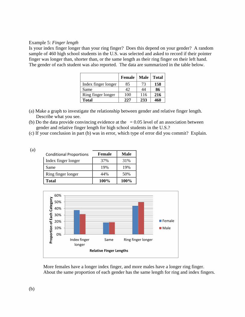
Example 5: Finger length
Is your index finger longer than your ring finger? Does this depend on your gender? A random
sample of 460 high school students in the U.S. was selected and asked to record if their pointer
finger was longer than, shorter than, or the same length as their ring finger on their left hand.
The gender of each student was also reported. The data are summarized in the table below.
Female Male Total
Index finger longer 85 73 158
Same 42 44 86
Ring finger longer 100 116 216
Total 227 233 460
(a) Make a graph to investigate the relationship between gender and relative finger length.
Describe what you see.
(b) Do the data provide convincing evidence at the = 0.05 level of an association between
gender and relative finger length for high school students in the U.S.?
(c) If your conclusion in part (b) was in error, which type of error did you commit? Explain.
(a)
More females have a longer index finger, and more males have a longer ring finger.
About the same proportion of each gender has the same length for ring and index fingers.
(b)
0%
10%
20%
30%
40%
50%
60%
Index fingerlonger
Same Ring finger longer
Pro
po
rtio
n o
f Ea
ch C
ate
gory
Relative Finger Lengths
Female
Male
Conditional Proportions Female Male
Index finger longer 37% 31%
Same 19% 19%
Ring finger longer 44% 50%
Total 100% 100%
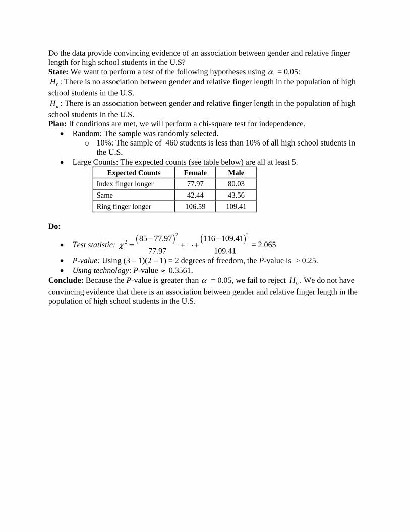
Do the data provide convincing evidence of an association between gender and relative finger
length for high school students in the U.S?
State: We want to perform a test of the following hypotheses using = 0.05:
0H : There is no association between gender and relative finger length in the population of high
school students in the U.S.
aH : There is an association between gender and relative finger length in the population of high
school students in the U.S.
Plan: If conditions are met, we will perform a chi-square test for independence.
Random: The sample was randomly selected.
o 10%: The sample of 460 students is less than 10% of all high school students in
the U.S.
Large Counts: The expected counts (see table below) are all at least 5.
Expected Counts Female Male
Index finger longer 77.97 80.03
Same 42.44 43.56
Ring finger longer 106.59 109.41
Do:
Test statistic:
2 2
285 77.97 116 109.41
77.97 109.41
= 2.065
P-value: Using (3 – 1)(2 – 1) = 2 degrees of freedom, the P-value is > 0.25.
Using technology: P-value 0.3561.
Conclude: Because the P-value is greater than = 0.05, we fail to reject 0H . We do not have
convincing evidence that there is an association between gender and relative finger length in the
population of high school students in the U.S.

Example 6: Glasses and Reading
Are avid readers more likely to wear glasses than those who read less frequently? Three hundred
men in the Korean army were selected at random and classified according to whether or not they
wore glasses and whether the amount of reading they did was above average, average, or below
average. The results are presented in the following table.
Wear Glasses?
Amount of Reading Yes No
Above average 47 26
Average 48 78
Below average 31 70
(a) Make a graph to investigate the relationship between amount of reading and wearing glasses
or not wearing glasses. Describe what you see.
(b) Do the data provide convincing evidence at the = 0.05 level of an association between
amount of reading and whether or not glasses are worn, for these Korean army men?
(c) If your conclusion in part (b) was in error, which type of error did you commit? Explain.
(a)
Conditional distribution in proportions:
Wear Glasses?
Amount of Reading Yes, Wears
Glasses
No, Does Not
Wear Glasses
Above average 0.37 0.15
Average 0.38 0.45
Below average 0.25 0.40
1 1
For above average readers, those who wear glasses have a much higher proportion than those
who do not wear glasses. For average readers, they have a more similar proportion although
non-glasses wearers is larger. For below-average reading, the non-glasses wearers have a much
higher proportion than those who wear glasses.
0.000.050.100.150.200.250.300.350.400.450.50
Aboveaverage
Average BelowaverageP
rop
ort
ion
Of
sam
ple
Ko
ren
Arm
y M
en
Amount of Reading
Yes, Wears Glasses
No, Does Not WearGlasses
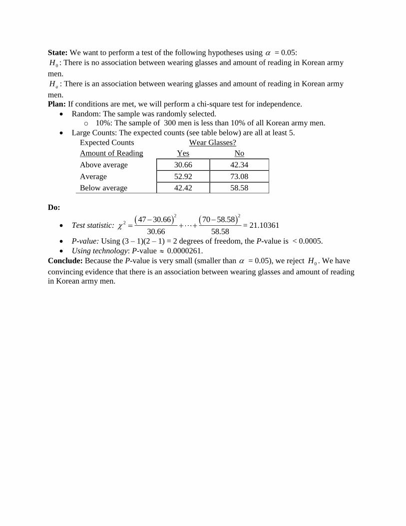
State: We want to perform a test of the following hypotheses using = 0.05:
0H : There is no association between wearing glasses and amount of reading in Korean army
men.
aH : There is an association between wearing glasses and amount of reading in Korean army
men.
Plan: If conditions are met, we will perform a chi-square test for independence.
Random: The sample was randomly selected.
o 10%: The sample of 300 men is less than 10% of all Korean army men.
Large Counts: The expected counts (see table below) are all at least 5.
Expected Counts Wear Glasses?
Amount of Reading Yes No
Above average 30.66 42.34
Average 52.92 73.08
Below average 42.42 58.58
Do:
Test statistic:
2 2
247 30.66 70 58.58
30.66 58.58
= 21.10361
P-value: Using (3 – 1)(2 – 1) = 2 degrees of freedom, the P-value is < 0.0005.
Using technology: P-value 0.0000261.
Conclude: Because the P-value is very small (smaller than = 0.05), we reject 0H . We have
convincing evidence that there is an association between wearing glasses and amount of reading
in Korean army men.
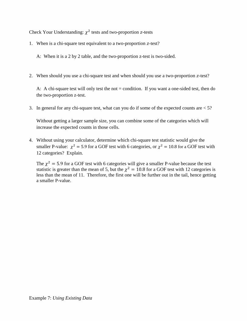
Check Your Understanding: tests and two-proportion -tests
1. When is a chi-square test equivalent to a two-proportion -test?
A: When it is a 2 by 2 table, and the two-proportion z-test is two-sided.
2. When should you use a chi-square test and when should you use a two-proportion -test?
A: A chi-square test will only test the not = condition. If you want a one-sided test, then do
the two-proportion z-test.
3. In general for any chi-square test, what can you do if some of the expected counts are < 5?
Without getting a larger sample size, you can combine some of the categories which will
increase the expected counts in those cells.
4. Without using your calculator, determine which chi-square test statistic would give the
smaller P-value: for a GOF test with 6 categories, or for a GOF test with
12 categories? Explain.
The for a GOF test with 6 categories will give a smaller P-value because the test
statistic is greater than the mean of 5, but the for a GOF test with 12 categories is
less than the mean of 11. Therefore, the first one will be further out in the tail, hence getting
a smaller P-value.
Example 7: Using Existing Data

An article in the Arizona Daily Star (April 9, 2009) included the following table. Suppose that
you decide to analyze these data using a chi-square test. However, without any additional
information about how the data were collected, it isn’t possible to know which chi-square test is
appropriate.
Age (years): 18–24 25–34 35–44 45–54 55–64 65+ Total
Use online social networks: 137 126 61 38 15 9 386
Do not use online social networks: 46 95 143 160 130 124 698
Total: 183 221 204 198 145 133 1084
(a) Explain why it is OK to use age as a categorical variable rather than a quantitative variable.
(b) Explain how you know that a goodness-of-fit test is not appropriate for analyzing these data.
(c) Describe how these data could have been collected so that a test for homogeneity is
appropriate.
(d) Describe how these data could have been collected so that a test for independence is
appropriate.
(a) Quantitative variables can be put into categories—but some info is lost.
(b) Since there are either two variables or two or more populations, a goodness-of-fit test
is not appropriate. Goodness-of-fit tests are appropriate only when analyzing the
distribution of one variable in one population.
(c) To make a test for homogeneity appropriate, we would need to take six independent
random samples, one from each age category, and then ask every person whether or not
they use online social networks. Or we could take two independent random samples, one
of online social network users and one of people who do not use online social networks,
and ask every member of each sample how old they are.
(d) To make a test for association/independence appropriate, we would take one random
sample from the population and ask every member about their age and whether or not
they use online social networks. This seems like the most reasonable method for
collecting the data, so a test of association/independence is probably the best choice. But
we can’t know for sure unless we know how the data were collected.
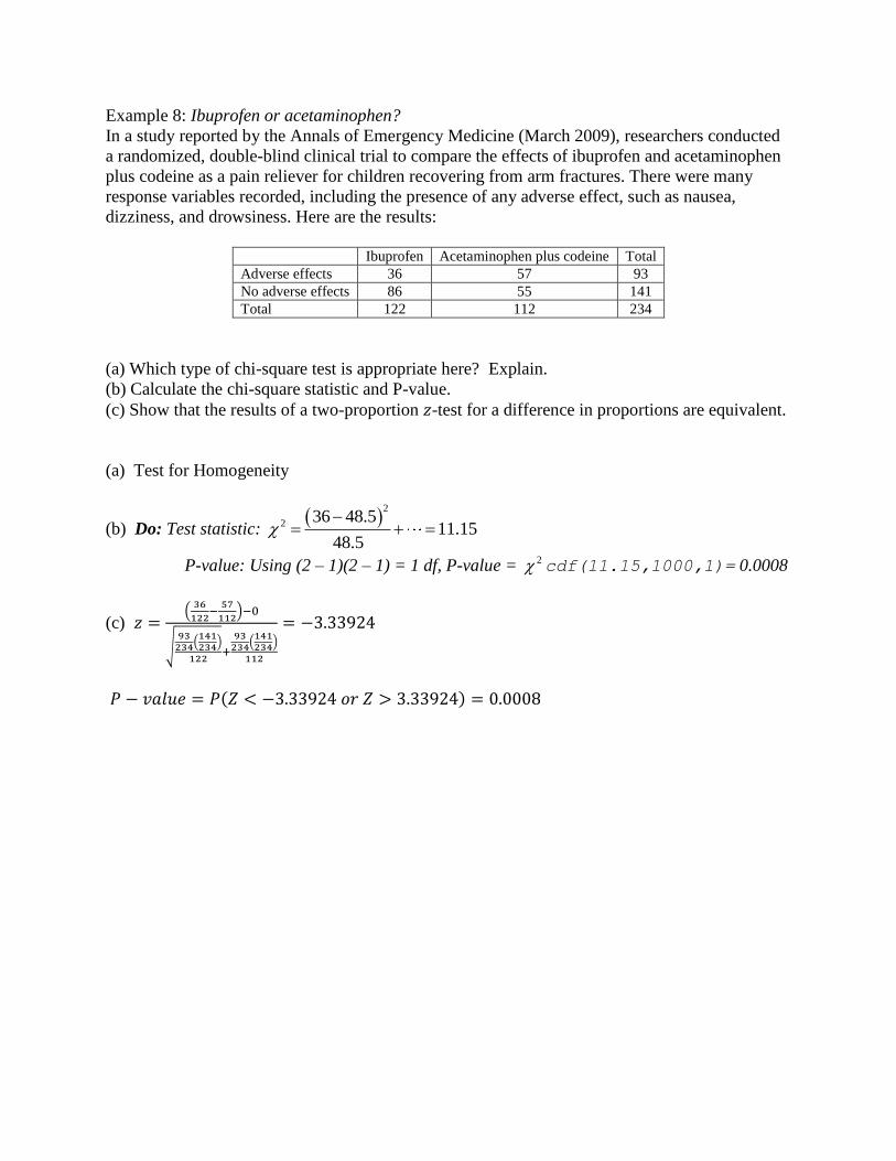
Example 8: Ibuprofen or acetaminophen?
In a study reported by the Annals of Emergency Medicine (March 2009), researchers conducted
a randomized, double-blind clinical trial to compare the effects of ibuprofen and acetaminophen
plus codeine as a pain reliever for children recovering from arm fractures. There were many
response variables recorded, including the presence of any adverse effect, such as nausea,
dizziness, and drowsiness. Here are the results:
Ibuprofen Acetaminophen plus codeine Total
Adverse effects 36 57 93
No adverse effects 86 55 141
Total 122 112 234
(a) Which type of chi-square test is appropriate here? Explain.
(b) Calculate the chi-square statistic and P-value.
(c) Show that the results of a two-proportion -test for a difference in proportions are equivalent.
(a) Test for Homogeneity
(b) Do: Test statistic:
2
2 36 48.511.15
48.5
P-value: Using (2 – 1)(2 – 1) = 1 df, P-value = 2 cdf(11.15,1000,1)= 0.0008
(c) (
)
√
(
)
(
)
( )