Embed Size (px)
Citation preview

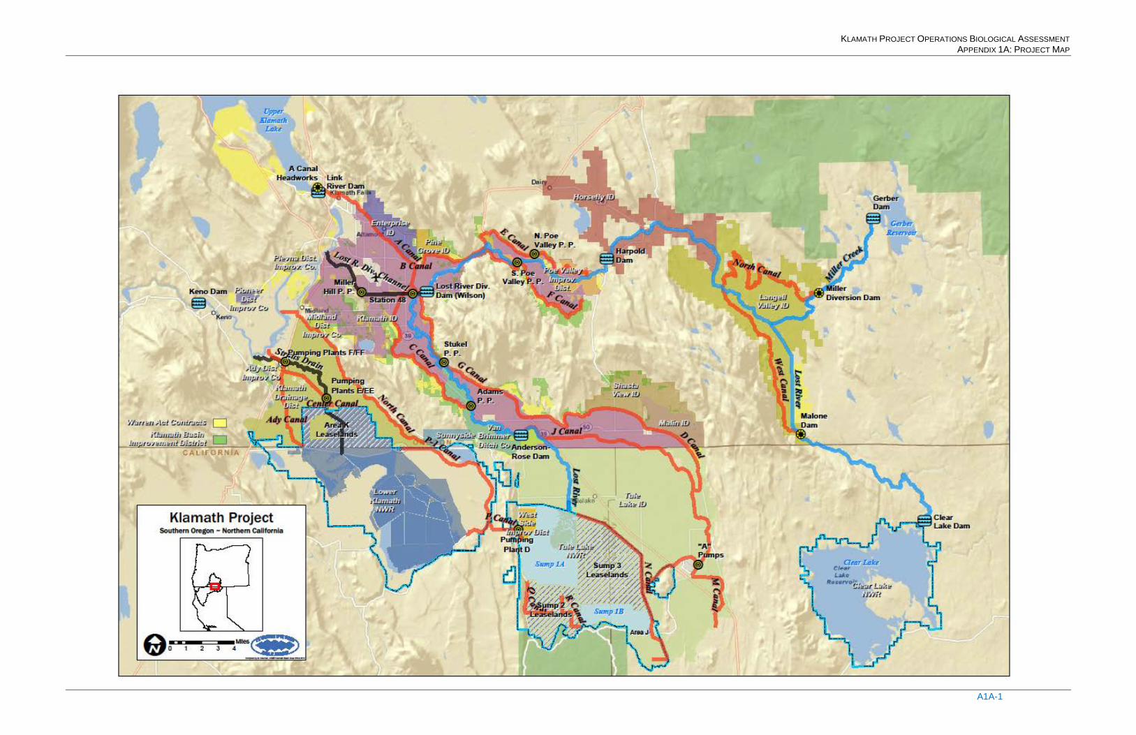
KLAMATH PROJECT OPERATIONS BIOLOGICAL ASSESSMENT APPENDIX 1A: PROJECT MAP
Appendix 1A: Project Map

KLAMATH PROJECT OPERATIONS BIOLOGICAL ASSESSMENT APPENDIX 1A: PROJECT MAP
KLAMATH PROJECT OPERATIONS BIOLOGICAL ASSESSMENT APPENDIX 1A: PROJECT MAP
A1A-1

KLAMATH PROJECT OPERATIONS BIOLOGICAL ASSESSMENT APPENDIX 1B: SPECIES LIST CORRESPONDENCE
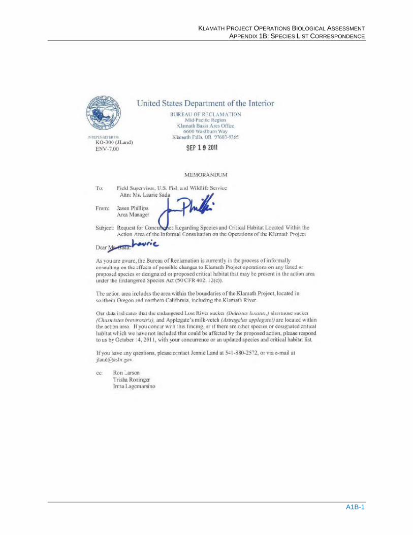
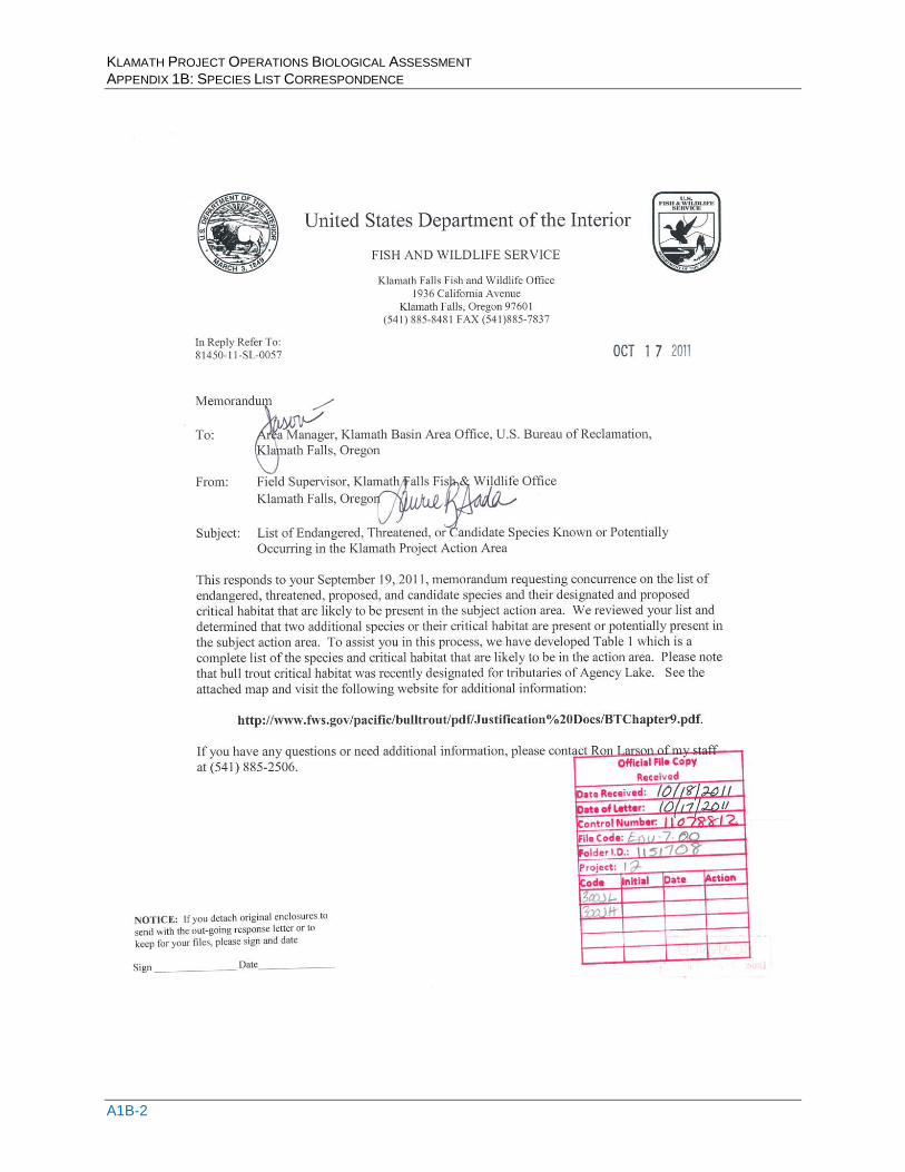
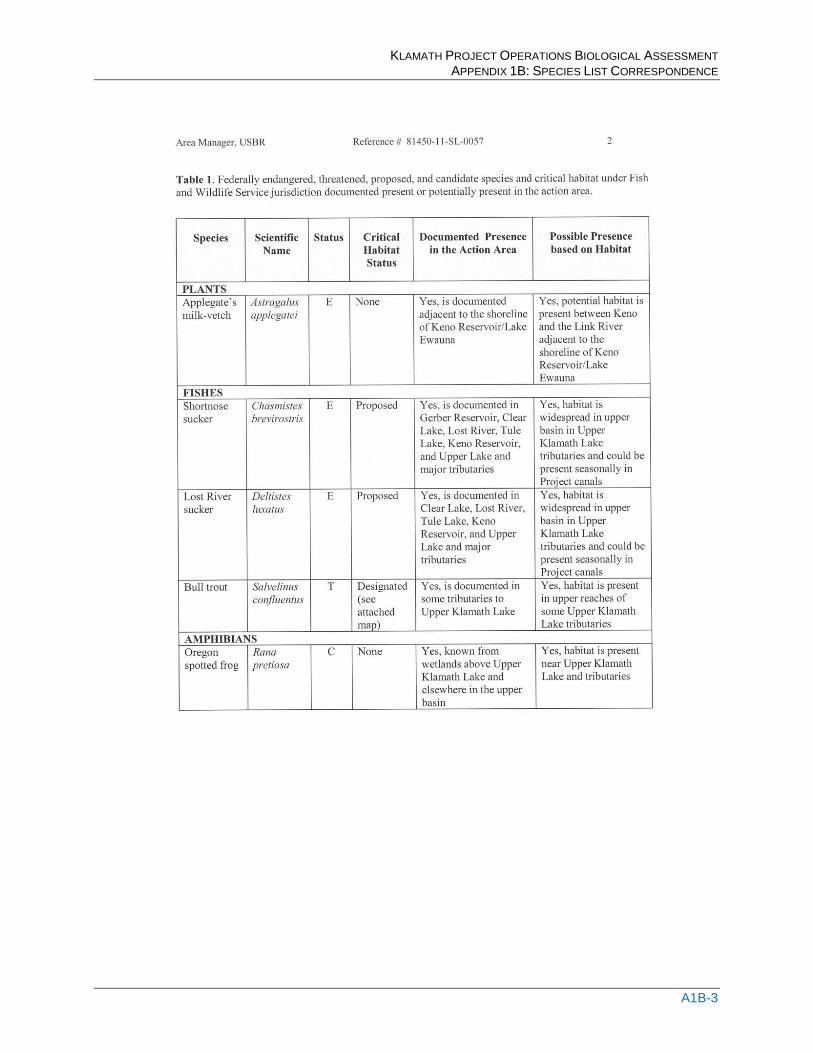
Appendix 1B: Species List Correspondence

KLAMATH PROJECT OPERATIONS BIOLOGICAL ASSESSMENT APPENDIX 1B: SPECIES LIST CORRESPONDENCE
KLAMATH PROJECT OPERATIONS BIOLOGICAL ASSESSMENT APPENDIX 1B: SPECIES LIST CORRESPONDENCE
A1B-1
KLAMATH PROJECT OPERATIONS BIOLOGICAL ASSESSMENT APPENDIX 1B: SPECIES LIST CORRESPONDENCE
A1B-2
KLAMATH PROJECT OPERATIONS BIOLOGICAL ASSESSMENT APPENDIX 1B: SPECIES LIST CORRESPONDENCE
A1B-3
KLAMATH PROJECT OPERATIONS BIOLOGICAL ASSESSMENT APPENDIX 1B: SPECIES LIST CORRESPONDENCE
A1B-4
KLAMATH PROJECT OPERATIONS BIOLOGICAL ASSESSMENT APPENDIX 1B: SPECIES LIST CORRESPONDENCE
A1B-5
KLAMATH PROJECT OPERATIONS BIOLOGICAL ASSESSMENT APPENDIX 1B: SPECIES LIST CORRESPONDENCE
A1B-6
KLAMATH PROJECT OPERATIONS BIOLOGICAL ASSESSMENT APPENDIX 1B: SPECIES LIST CORRESPONDENCE
A1B-7
KLAMATH PROJECT OPERATIONS BIOLOGICAL ASSESSMENT APPENDIX 1B: SPECIES LIST CORRESPONDENCE
A1B-8
KLAMATH PROJECT OPERATIONS BIOLOGICAL ASSESSMENT APPENDIX 1B: SPECIES LIST CORRESPONDENCE
A1B-9
KLAMATH PROJECT OPERATIONS BIOLOGICAL ASSESSMENT APPENDIX 1B: SPECIES LIST CORRESPONDENCE
A1B-10

KLAMATH PROJECT OPERATIONS BIOLOGICAL ASSESSMENT APPENDIX 4A: PROPOSED ACTION DEVELOPMENT
Appendix 4A Proposed Action Development
Appendix 4A-1: Model Documentation

KLAMATH PROJECT OPERATIONS BIOLOGICAL ASSESSMENT APPENDIX 4A: PROPOSED ACTION DEVELOPMENT
KLAMATH PROJECT OPERATIONS BIOLOGICAL ASSESSMENT APPENDIX 4A: PROPOSED ACTION DEVELOPMENT
A4A-1
Appendix 4A-1
Contents A.4.1 Model Overview A.4.2 WRIMS and WRESL Code A.4.3 Model Representation
A.4.3.1 Modeled Rivers, Lakes, Conveyance Facilities and Model Schematic A.4.3.2 Period of Record A.4.3.3 Hydrology Inputs
A.4.3.3.1 Definitions A.4.3.3.2 Datasets A.4.3.3.3 Project Daily Data and Project Historic Use Data A.4.3.3.4 Upper Klamath Lake Net Inflows A.4.3.3.5 Lake Ewauna Accretions A.4.3.3.6 Keno Dam to Iron Gate Dam Accretions A.4.3.3.7 Lost River Diversion Channel Inflow from Lost River A.4.3.3.8 Area 2 Winter Runoff A.4.3.3.9 Natural Resources Conservation Service Forecasts
A.4.3.4 Key Model Variables A.4.4 Simulated Operations
A.4.4.1 Fall-Winter Operations A.4.4.2 Spring-Summer Operations A.4.4.3 Project Supply Use in Model A.4.4.4 Project Return Flows A.4.4.5 EWA Use in Model A.4.4.6 EWA and Flood Control Releases A.4.4.7 Refuge Operation A.4.4.8 Flood Control Operations A.4.4.9 Flow Ramping
KLAMATH PROJECT OPERATIONS BIOLOGICAL ASSESSMENT APPENDIX 4A: PROPOSED ACTION DEVELOPMENT
A4A-2
FIGURES Figure A.4.1.1 Location of Upper Klamath Basin, Oregon and California, and Locations of Major Rivers Figure A.4.3.1 Klamath Projects, Oregon and California Figure A.4.3.2 Model Schematic Figure A.4.4.7.1 Percentage of Remaining Project Supply to Refuge TABLES Table A.4.3.4.1 Key Model Variables Table A.4.4.1.1 Link River Dam Minimum Flow Release Table A.4.4.1.2 Iron Gate Minimum Flow Release Table A.4.4.1.3 Fill Rate Adjustment Factor Table A.4.4.1.4 Williamson River Release Target Proportion Table A.4.4.1.5 Net Accretion Adjustment Factor Table A.4.4.1.6 Calculation of Fall/Winter Link River Dam Release Target Table A.4.4.2.1 Elevation Storage-Area Table A.4.4.2.2 End of September UKL Storage Target Table A.4.4.2.3 EWA Percentages Table A.4.4.3.1 Historical Project Demand from 1980 - 2011 Table A.4.4.3.2 Distribution Type Table A.4.4.3.3 Distribution Patterns for A Canal Portion of the Supply Table A.4.4.3.4 Distribution Patterns for Station 48 and Miller Hill Portion of the Supply Table A.4.4.3.5 Distribution Patterns for North Canal Portion of the Supply Table A.4.4.3.6 Distribution Patterns for Ady Canal (Ag Only) Portion of the Supply Table A.4.4.5.1 EWA Reserves Table A.4.4.5.2 Monthly Iron Gate Minimum In-stream Flow Table A.4.4.5.3 Absolute Maximum Flow for the Klamath River by Month Table A.4.4.7.1 Monthly Refuge Demand and UKL Elevation Thresholds Which Condition Refuge Delivery Table A.4.4.7.2 Upper Klamath Lake and Refuge Adjustment Threshold Table A.4.4.1 UKL Flood Release Threshold Elevations for the Last Day of Each Month Under Relatively Dry or Wet Conditions Table A.4.4.8.1 UKL Flood Release Threshold Elevations for the Last Day of Each Month Under Relatively Dry or Wet Conditions
KLAMATH PROJECT OPERATIONS BIOLOGICAL ASSESSMENT APPENDIX 4A: PROPOSED ACTION DEVELOPMENT
A4A-3
Section A - Key Model Variables Table A.4.3.4.1 Key Model Variables Section B - Proposed Action Model Output Graphs Figure B1. Modeled versus Historic Iron Gate Flows and Upper Klamath Lake Elevations (1981-1983) Figure B2. Modeled versus Historic Iron Gate Flows and Upper Klamath Lake Elevations (1984-1986) Figure B3. Modeled versus Historic Iron Gate Flows and Upper Klamath Lake Elevations (1987-1989) Figure B4. Modeled versus Historic Iron Gate Flows and Upper Klamath Lake Elevations (1990-1992) Figure B5. Modeled versus Historic Iron Gate Flows and Upper Klamath Lake Elevations (1993-1995) Figure B6. Modeled versus Historic Iron Gate Flows and Upper Klamath Lake Elevations (1996-1998) Figure B7. Modeled versus Historic Iron Gate Flows and Upper Klamath Lake Elevations (1999-2001) Figure B8. Modeled versus Historic Iron Gate Flows and Upper Klamath Lake Elevations (2002-2004) Figure B9. Modeled versus Historic Iron Gate Flows and Upper Klamath Lake Elevations (2005-2007) Figure B10. Modeled versus Historic Iron Gate Flows and Upper Klamath Lake Elevations (2008-2010) Figure B11. Modeled versus Historic Iron Gate Flows and Upper Klamath Lake Elevations (2011) Figure B12. Modeled Annual Diversions versus Historic Diversions from All Sources Figure B13. Modeled Spring/Summer (Mar-Nov) Deliveries versus Historic Deliveries from All Sources Figure B14. Modeled Fall/Winter Deliveries versus Historic Deliveries from All Sources Figure B15. Modeled Annual Deliveries versus Historic Deliveries to Refuge Figure B16. Modeled Summer Deliveries versus Historic Deliveries to Refuge Figure B17. Modeled Winter Deliveries versus Historic Deliveries to Refuge Section C - Lower Klamath NWR Historic Deliveries Table C1. Historic Lower Klamath NWR Water Deliveries Figure C1. Historic Lower Klamath NWR Water Deliveries Section D - Clear Lake and Gerber Water Supply Forecast Models Table D1. Clear Lake Operational Forecast Model (April 1 – 50% Exceedance) Table D2. Clear Lake Operational Forecast Model (April 1 – 70% Exceedance) Table D3. Clear Lake Operational Forecast Model (April 1 – 90% Exceedance) Table D4. Gerber Reservoir Operational Forecast Model (April 1 – 50% Exceedance) Table D5. Gerber Reservoir Operational Forecast Model (April 1 – 70% Exceedance) Table D6. Gerber Reservoir Operational Forecast Model (April 1 – 90% Exceedance)
KLAMATH PROJECT OPERATIONS BIOLOGICAL ASSESSMENT APPENDIX 4A: PROPOSED ACTION DEVELOPMENT
A4A-4
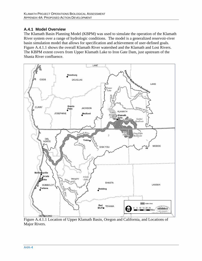
A.4.1 Model Overview The Klamath Basin Planning Model (KBPM) was used to simulate the operation of the Klamath River system over a range of hydrologic conditions. The model is a generalized reservoir-river basin simulation model that allows for specification and achievement of user-defined goals. Figure A.4.1.1 shows the overall Klamath River watershed and the Klamath and Lost Rivers. The KBPM extent covers from Upper Klamath Lake to Iron Gate Dam, just upstream of the Shasta River confluence.
Figure A.4.1.1 Location of Upper Klamath Basin, Oregon and California, and Locations of Major Rivers.
KLAMATH PROJECT OPERATIONS BIOLOGICAL ASSESSMENT APPENDIX 4A: PROPOSED ACTION DEVELOPMENT
A4A-5
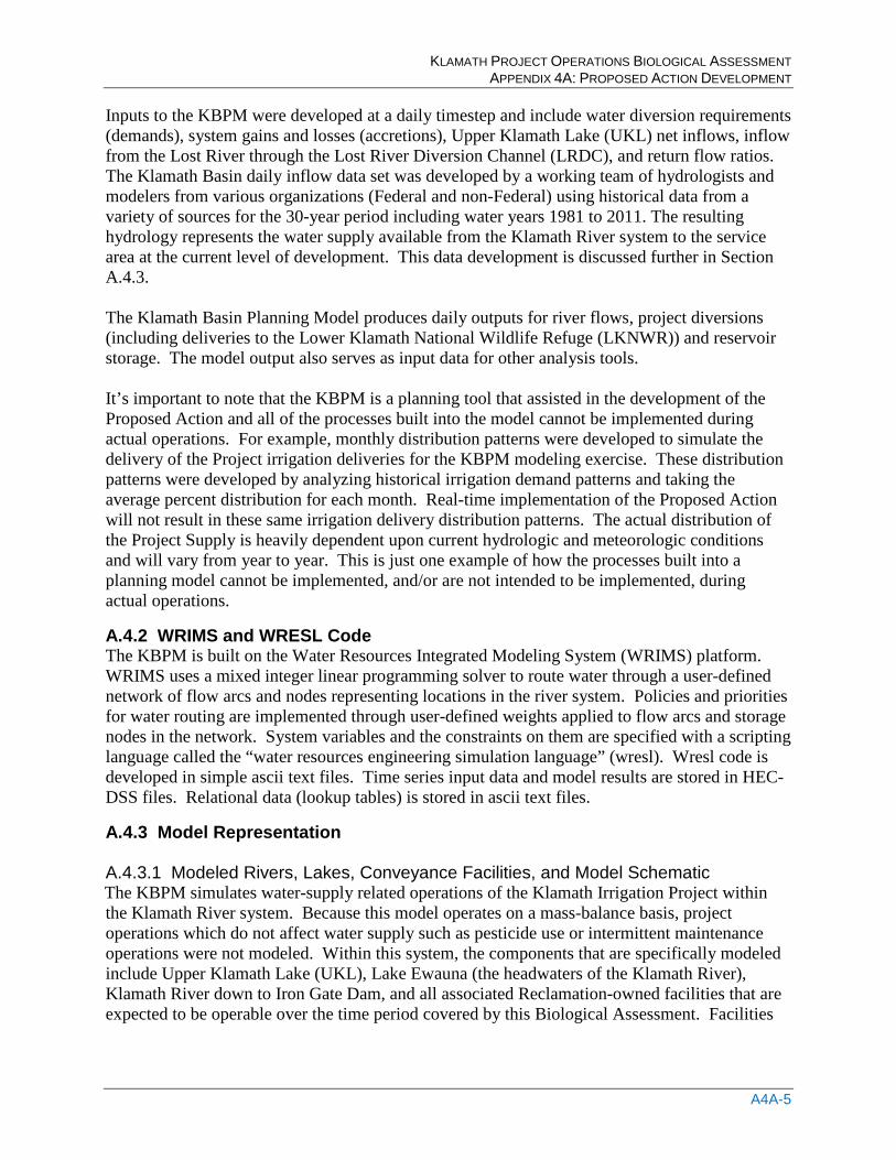
Inputs to the KBPM were developed at a daily timestep and include water diversion requirements (demands), system gains and losses (accretions), Upper Klamath Lake (UKL) net inflows, inflow from the Lost River through the Lost River Diversion Channel (LRDC), and return flow ratios. The Klamath Basin daily inflow data set was developed by a working team of hydrologists and modelers from various organizations (Federal and non-Federal) using historical data from a variety of sources for the 30-year period including water years 1981 to 2011. The resulting hydrology represents the water supply available from the Klamath River system to the service area at the current level of development. This data development is discussed further in Section A.4.3. The Klamath Basin Planning Model produces daily outputs for river flows, project diversions (including deliveries to the Lower Klamath National Wildlife Refuge (LKNWR)) and reservoir storage. The model output also serves as input data for other analysis tools. It’s important to note that the KBPM is a planning tool that assisted in the development of the Proposed Action and all of the processes built into the model cannot be implemented during actual operations. For example, monthly distribution patterns were developed to simulate the delivery of the Project irrigation deliveries for the KBPM modeling exercise. These distribution patterns were developed by analyzing historical irrigation demand patterns and taking the average percent distribution for each month. Real-time implementation of the Proposed Action will not result in these same irrigation delivery distribution patterns. The actual distribution of the Project Supply is heavily dependent upon current hydrologic and meteorologic conditions and will vary from year to year. This is just one example of how the processes built into a planning model cannot be implemented, and/or are not intended to be implemented, during actual operations.
A.4.2 WRIMS and WRESL Code The KBPM is built on the Water Resources Integrated Modeling System (WRIMS) platform. WRIMS uses a mixed integer linear programming solver to route water through a user-defined network of flow arcs and nodes representing locations in the river system. Policies and priorities for water routing are implemented through user-defined weights applied to flow arcs and storage nodes in the network. System variables and the constraints on them are specified with a scripting language called the “water resources engineering simulation language” (wresl). Wresl code is developed in simple ascii text files. Time series input data and model results are stored in HEC-DSS files. Relational data (lookup tables) is stored in ascii text files.
A.4.3 Model Representation A.4.3.1 Modeled Rivers, Lakes, Conveyance Facilities, and Model Schematic The KBPM simulates water-supply related operations of the Klamath Irrigation Project within the Klamath River system. Because this model operates on a mass-balance basis, project operations which do not affect water supply such as pesticide use or intermittent maintenance operations were not modeled. Within this system, the components that are specifically modeled include Upper Klamath Lake (UKL), Lake Ewauna (the headwaters of the Klamath River), Klamath River down to Iron Gate Dam, and all associated Reclamation-owned facilities that are expected to be operable over the time period covered by this Biological Assessment. Facilities
KLAMATH PROJECT OPERATIONS BIOLOGICAL ASSESSMENT APPENDIX 4A: PROPOSED ACTION DEVELOPMENT
A4A-6
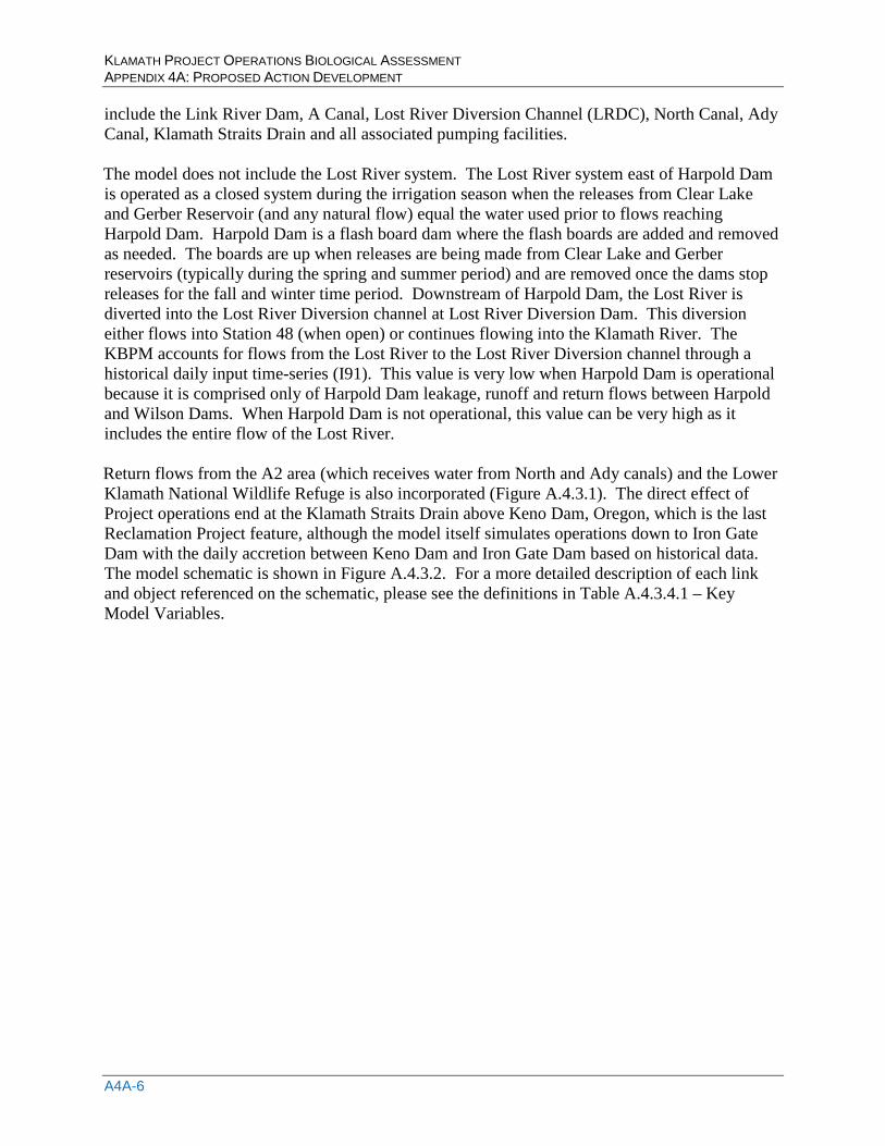
include the Link River Dam, A Canal, Lost River Diversion Channel (LRDC), North Canal, Ady Canal, Klamath Straits Drain and all associated pumping facilities. The model does not include the Lost River system. The Lost River system east of Harpold Dam is operated as a closed system during the irrigation season when the releases from Clear Lake and Gerber Reservoir (and any natural flow) equal the water used prior to flows reaching Harpold Dam. Harpold Dam is a flash board dam where the flash boards are added and removed as needed. The boards are up when releases are being made from Clear Lake and Gerber reservoirs (typically during the spring and summer period) and are removed once the dams stop releases for the fall and winter time period. Downstream of Harpold Dam, the Lost River is diverted into the Lost River Diversion channel at Lost River Diversion Dam. This diversion either flows into Station 48 (when open) or continues flowing into the Klamath River. The KBPM accounts for flows from the Lost River to the Lost River Diversion channel through a historical daily input time-series (I91). This value is very low when Harpold Dam is operational because it is comprised only of Harpold Dam leakage, runoff and return flows between Harpold and Wilson Dams. When Harpold Dam is not operational, this value can be very high as it includes the entire flow of the Lost River. Return flows from the A2 area (which receives water from North and Ady canals) and the Lower Klamath National Wildlife Refuge is also incorporated (Figure A.4.3.1). The direct effect of Project operations end at the Klamath Straits Drain above Keno Dam, Oregon, which is the last Reclamation Project feature, although the model itself simulates operations down to Iron Gate Dam with the daily accretion between Keno Dam and Iron Gate Dam based on historical data. The model schematic is shown in Figure A.4.3.2. For a more detailed description of each link and object referenced on the schematic, please see the definitions in Table A.4.3.4.1 – Key Model Variables.
KLAMATH PROJECT OPERATIONS BIOLOGICAL ASSESSMENT APPENDIX 4A: PROPOSED ACTION DEVELOPMENT
A4A-7
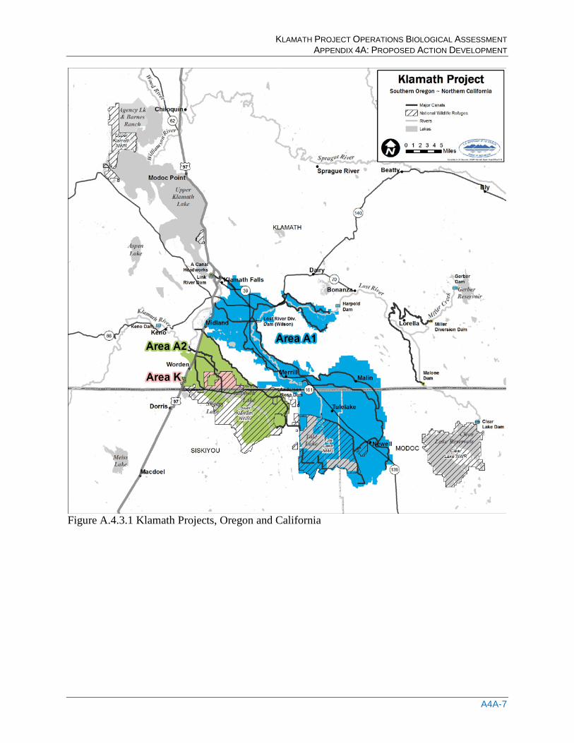
Figure A.4.3.1 Klamath Projects, Oregon and California
KLAMATH PROJECT OPERATIONS BIOLOGICAL ASSESSMENT APPENDIX 4A: PROPOSED ACTION DEVELOPMENT
A4A-8
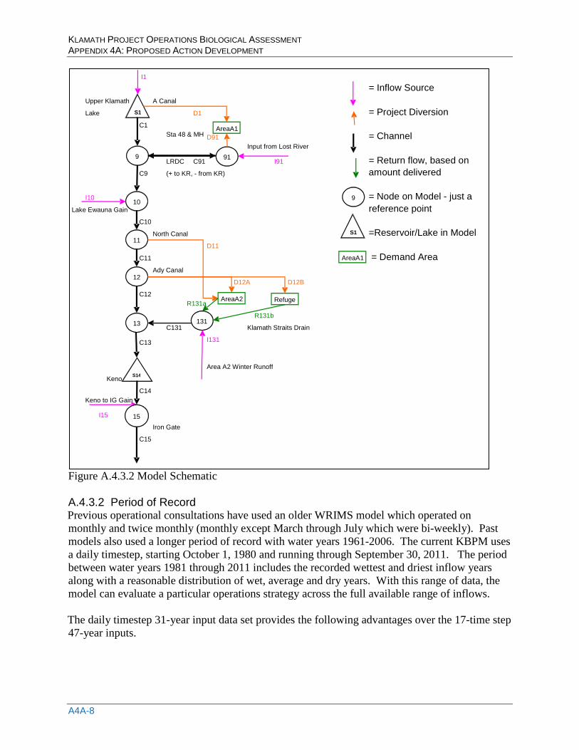
Figure A.4.3.2 Model Schematic A.4.3.2 Period of Record Previous operational consultations have used an older WRIMS model which operated on monthly and twice monthly (monthly except March through July which were bi-weekly). Past models also used a longer period of record with water years 1961-2006. The current KBPM uses a daily timestep, starting October 1, 1980 and running through September 30, 2011. The period between water years 1981 through 2011 includes the recorded wettest and driest inflow years along with a reasonable distribution of wet, average and dry years. With this range of data, the model can evaluate a particular operations strategy across the full available range of inflows. The daily timestep 31-year input data set provides the following advantages over the 17-time step 47-year inputs.
I1 = Inflow Source
Upper Klamath A Canal Lake D1 = Project Diversion
C1 Sta 48 & MH D91 = Channel
Input from Lost River LRDC C91 I91 = Return flow, based on
C9 (+ to KR, - from KR) amount delivered
I10 = Node on Model - just a Lake Ewauna Gain reference point
C10 North Canal =Reservoir/Lake in Model
D11 C11 = Demand Area
Ady Canal D12A D12B
C12 R131a
R131b C131 Klamath Straits Drain
C13 I131
Area A2 Winter Runoff Keno
C14 Keno to IG Gain
I15 Iron Gate
C15
S1 AreaA1
10
S14
9
11
12
13
AreaA2 Refuge
131
91
15
9
S1
AreaA1
KLAMATH PROJECT OPERATIONS BIOLOGICAL ASSESSMENT APPENDIX 4A: PROPOSED ACTION DEVELOPMENT
A4A-9
• Essential daily data inputs are available electronically for water years 1981-2011. Daily data for 1961-1980 is not in a usable format and would require extensive reprocessing and review before it could be used for modeling.
• Updated forecasts from the Natural Resources Conservation Service (NRCS) for March, April, May and June are only available from 1981-2011. These forecasts were updated based on the new, current forecasting methods and therefore better reflect how the proposed operation (which is based heavily on forecasts) would affect overall water conditions.
• 1981-2011 still includes the widest range of hydrologic conditions (lowest (1992) and highest (1983) inflow years), and includes various multi-year hydrologic cycles:
o Oscillating extreme years such as 2005/2006/2007 where UKL net inflows for April-September measured 360/758/358 thousand acre-feet (TAF), respectively.
o Repetitive wetter years such as 1982/1983/1984 where UKL net inflows for April-September measured 721/895/839 TAF, respectively.
o Repetitive drier years such as 2001/2002/2003 where UKL net inflows for April-September measured 242/341/373 TAF, respectively.
A.4.3.3 Hydrology Inputs A.4.3.3.1 Definitions Quality Assurance is process oriented: to make sure the correct things are done in the correct manner. Planned and systematic activities implemented in a quality system so that quality requirements for a product or service will be fulfilled. In the context of data sets for the WRIMS model, quality assurance will relate to the configuration of the physical infrastructure of water diversions structures, gauging systems, and how data are collected. Quality Control is product oriented: to make sure the results meet the expectations of the Project. It includes the techniques and activities used to fulfill requirements for quality. QC emphasizes testing of products to uncover defects. In the context of data sets for the WRIMS model, quality control will relate to proofing of the data and correcting/adjusting data so that a final reliable dataset is created. A.4.3.3.2 Data Sets 1. Project Daily Data and Project Historic Use Data 2. Upper Klamath Lake net inflow 3. Lake Ewauna accretions 4. Keno Dam to Iron Gate accretions 5. Lost River Diversion Channel inflow from the Lost River 6. Area 2 winter runoff 7. Natural Resource Conservation Service forecasts 8. Crater Lake precipitation
A.4.3.3.3 Project Daily Data and Project Historic Use Data Electronic data from sources listed below were combined into one file and compared to a 2010 version of Reclamation’s MODSUM file. The electronic data were then compared with hard
KLAMATH PROJECT OPERATIONS BIOLOGICAL ASSESSMENT APPENDIX 4A: PROPOSED ACTION DEVELOPMENT
A4A-10
copies of Klamath Irrigation Project Daily Operations Reports. Comparison was completed on a day by day basis for A Canal, Lost River Diversion Channel (LRDC) total flow, Station 48, Miller Hill Pump, Miller Hill Spill, ungauged Klamath Irrigation District pumping plants, North Canal, Ady Canal, Ady Canal to Lower Klamath Lake Refuge, Klamath Straits Drain, F pump, FF pump, and ungauged Area 2 diversions. Quality control of the project data began with the following electronic Excel files provided by Reclamation: KHYDRODBA_1994-2010_Crop_Averages KHYDRODBA_ADYCANAL KHYDRODBA_ADYREFUGE KHYDRODBA_KIDPUMPS KHYDRODBA_KSCHAN KHYDRODBA_LRDCHAN KHYDRODBA_NORTHCAN KHYDRODBA_PUMPF_FF KHYDRODBA_TIDSTUFF KHYDRODBA_UKLDATA KHYDRODBA_WESTCAN Klamath_Project_Drainage_Through_TID Pacificorps_KLA_0506_Flows_REV The quality controlled daily project dataset was finalized for October 1, 1974 through September 30, 2011 for Area 1, and January 1, 1980 through September 30, 2011 for Area 2. For Water Year 2011, data after December 25, 2010 are from electronic records and were not checked against hard copy Daily Operations Reports because the reports had not been prepared. Where differences existed between the hard copy and electronic data, hard copy Operations Reports were assumed to be correct and the electronic records were modified to match the Operations Reports. Short (1 to 3 days) data gaps were filled with synthesized data generated using linear interpolation. Longer data gaps were filled using other Reclamation or water district records. Within the KBPM, the Historic Project Use table has been updated several times as new and revised data have been included. Updates include adding ungauged Area 1 data, ungauged Area 2 data, revisions to the Station 48 data, and minor corrections to calculation of historic project use. The most recent update was in August 2012 to incorporate revised water bank values between 2001 and 2010. The WRIMS model uses project data as yearly sums for the period of record in a lookup table. However, the raw daily project data, or subsets, are used in calculating UKL net inflow, Lake Ewauna accretions, and LRDC inflow from the Lost River. Project daily data are contained in the spreadsheet: Daily_Project_diversions_1975-2011(A1)_1980-2011(A2)_DRAFT_June_25_2012.xlsx. Project historic use data are contained in the spreadsheet: HisAgUseCalcs_rev_June_25_2012.xlsx. In WRIMS, historic use data are contained in the file: histprjuse.table.
KLAMATH PROJECT OPERATIONS BIOLOGICAL ASSESSMENT APPENDIX 4A: PROPOSED ACTION DEVELOPMENT
A4A-11
A.4.3.3.4 Upper Klamath Lake Net Inflow The Upper Klamath Lake (UKL) daily net inflow dataset is calculated from quality-controlled data for (1) A Canal diversions (Reclamation), (2) average daily flows for the Link River at Link River Dam (USGS), (3) Westside Power Canal (often referred to as the Keno Canal) flows (PacifiCorp), (4) Agency Lake Ranch and Caledonia operations (Reclamation), and (5) active storage data for UKL (Reclamation). Additional minor revisions will be required because in July and August 2012 Reclamation recalculated Agency Lake Ranch data, based on revised pump efficiency curves. Storage volume in UKL is dependent on the elevation of the lake surface and the capacity of the lake, and the capacity has varied over time. The UKL net inflow dataset elevation-capacity relationships are as follows:
• October 1, 1980 through July 7, 2006: UKL without Caledonia, Tulana, or Goose Bay • July 7, 2006 through December 31, 2006: UKL with Caledonia • January 1, 2007 through October 30, 2007: UKL without Caledonia, Tulana, or Goose Bay • October 31, 2007 through November 17, 2008: UKL with Tulana • November 18, 2008 through September 30, 2011: UKL with Tulana and Goose Bay The UKL daily net inflow is calculated using the following equation: Net Inflow = {(UKL storage volume today – UKL storage volume yesterday) + (Link River + Westside Canal) + (A Canal) + (Volume pumped to Agency Lake Ranch [positive] Or {(Volume pumped from Agency Lake Ranch [negative]) – (Volume from Caledonia Marsh)}. The KBPM uses both raw daily data and a 3-day moving average of the daily data for UKL inflow. The raw daily data input variable is I1_raw and is used in a calculation of cumulative inflow into UKL. The moving average of the previous 3 days of inflow input variable is I1 and defines the Available Inflow above Link River Dam (AIL) term used in the Fall-Winter River Operations, as well as providing the inflow element of the mass balance equation for UKL. Upper Klamath Lake net inflow data are contained in the spreadsheet: UKL_DailyNetInflow_FINAL_21May2012.xlsx. In KBPM, the time series’ I1_raw and I1, for UKL daily net inflow and 3-day moving average data are contained in the file: DailyPA_SV.dss. Upper Klamath Lake head-area-capacity data for the current configuration of UKL are contained in the spreadsheet: ReservoirInfoLookupTables_FINAL_updated-02May2012.xlsx. In KBPM, this data is contained in the files: res_info.table and res_info2.table. A.4.3.3.5 Lake Ewauna Accretions The Lake Ewauna daily accretion dataset is calculated from quality controlled data for (1) LRDC spill to the Klamath River, (2) LRDC delivery to Area 1 from the Klamath River, (3) pumps F and FF, (4) North Canal, (5) Ady Canal, (6) Unguaged Area 2 diversions, (7) PacifiCorp data for the Westside Power Canal, and (8) USGS average daily flow data for Link River at Link River Dam and Klamath River at Keno Dam. The Lake Ewauna accretions are calculated using the following equations: Accretions = (Measured Keno Flow) – (Computed Keno Flow), and
KLAMATH PROJECT OPERATIONS BIOLOGICAL ASSESSMENT APPENDIX 4A: PROPOSED ACTION DEVELOPMENT
A4A-12
Computed Keno Flow = [(Link River + Westside Canal) + (LRDC spill to the Klamath River) + (Pumps F and FF) – (LRDC delivery to Area 1 from the Klamath River) – (North Canal) – (Ady Canal) – Ungauged Area 2 diversions)] The WRIMS model uses a 3-day moving average of the daily Lake Ewauna accretion data. The input variable is I10. Lake Ewauna accretions data are contained in the spreadsheet: Lake Ewauna accretions FINAL May 21 2012.xlsx. In KBPM, Lake Ewauna accretion data are contained in the file: DailyPA_SV.dss. A.4.3.3.6 Keno Dam to Iron Gate Dam Accretions The Keno Dam to Iron Gate Dam daily accretion dataset is calculated from USGS average daily flow gage data for the Klamath River at Keno Dam and Iron Gate Dam, and the Scott and Shasta Rivers. The accretion value was proportioned on Scott and Shasta River flows to impose a reasonably normative yearly hydrograph on the Klamath River reach between Keno and Iron Gate dams, which is highly regulated and includes several reservoirs. Average daily flow (cubic feet per second [cfs]) data for the Scott and Shasta rivers were converted to average daily volume (thousands of acre-feet [TAF]) using the following equation: Thousands of acre-feet = (flow in cfs) * [(86,400 seconds per day) / (43,560 cubic feet per acre-foot) / (1,000)]. The daily volume data for each river were then divided by the total monthly volume for that respective river to develop a proportional volume for each day of the month for each river. The daily proportional volume for each river was then multiplied by the monthly volume of accretions between Keno Dam and Iron Gate Dam to develop two sets of accretions between Keno and Iron Gate: one proportioned to the Scott River and one proportioned to the Shasta River. The two sets of proportioned accretion data were then averaged to create one dataset of daily accretions between Keno Dam and Iron Gate Dam. The KBPM model uses a 5-day moving average of the daily proportioned Keno Dam to Iron Gate Dam accretion data. The input variable is I15. Keno Dam to Iron Gate Dam accretions data are contained in the spreadsheet: KenoIGDAccretionsDaily_30Sep2011_FINAL.xlsx. In KBPM, Keno Dam to Iron Gate Dam accretion data are contained in the file: DailyPA_SV.dss. A.4.3.3.7 Lost River Diversion Channel Inflow From Lost River Lost River return flows are diverted into the Lost River Diversion Channel at the Lost River Diversion Dam. Data for these return flows are included in the QA/QC’ed Daily_Project_diversions_1975-2011(A1)_1980-2011(A2)_DRAFT_June_25_2012.xls dataset.. A.4.3.3.8 Area 2 Winter Runoff The Area A2 Winter Runoff data input was added as a water balancing term to ensure all water remained within the system. The name of this data value originated in previous models and was retained for continuity; however this value represents more than only winter runoff. This data value is simply the difference of actual, historical pumped return flow at pumping plants F and
KLAMATH PROJECT OPERATIONS BIOLOGICAL ASSESSMENT APPENDIX 4A: PROPOSED ACTION DEVELOPMENT
A4A-13
FF and known values that discharged into the Straits Drain. Pumping plants F and FF pump water from the Straits Drain into the Klamath River and receive direct discharge from the LKNWR as well as return flows from project area A2. In the winter and spring, precipitation events may create runoff that also drains into the Straits Drain from any point along the drain. In addition, gage errors, changes in pumping efficiency, changes in canal dimensions and increased or decreased efficiency in area A2 water use could all contribute to this balancing term. This formula is as follows: A2 Winter Runoff = F/FF – LKNWR@Stateline - (%Return*A2 Deliveries) The % return value is discussed later in the documentation in Section 4.4.5, but is equal to 30% or 40% depending on the month. This value was updated from previous models in late 2011 and was not updated with the corrected daily historical deliveries that were developed during 2012, as explained in other sections. Therefore, this value was calculated on a monthly basis as the monthly volume pumped at pumping plants F and FF less the expected return flow from A2 less the LKNWR monthly return flows at Stateline Road. These values were divided by the number of days in each month in order to incorporate into the daily time step WRIMS model. A.4.3.3.9 Natural Resources Conservation Service Forecasts The Natural Resources Conservation Service (NRCS) provided reconstructed UKL net inflow forecasts for water years 1981 through 2011 using the most recent version of the UKL calculated net inflow data (see above). The most recent reconstructed forecasts were completed by NRCS in April 2012. NRCS forecast reconstructions are contained in the spreadsheet: NRCS_Klamath_forecast_reconstructions_FINAL_11Apr2012.xlsx. In KBPM, NRCS forecast data are contained in the file: forecasts50pct.table. A.4.3.4 Key Model Variables In many cases, the actual variables used in the model code have names which are not clearly descriptive of their definition. This is a function of multiple model developers, changing intentions and strategies and general model adaptation. In order to connect the actual model code to the operations described below, please use the table of key model variables listed in Table A.4.3.4.1. This table provides an overview definition of each key variable with a common name (as referenced in the operations sections below) and location within the model files. Due to size, this table is located in Section A found at the end of this document.
A.4.4 Simulated Operations A.4.4.1 Fall-Winter Operations The Fall-Winter Klamath Project Rules of Operation are intended to divide the available Fall-Winter water supply between the following competing goals: 1. Fill UKL for the upcoming irrigation season and critical fish habitat needs. 2. Release sufficient flow from Link Dam to meet downstream fish needs.
KLAMATH PROJECT OPERATIONS BIOLOGICAL ASSESSMENT APPENDIX 4A: PROPOSED ACTION DEVELOPMENT
A4A-14
3. Meet Fall-Winter project demands: a. Klamath Drainage District (Area A2 – serviced by North Canal and Ady Canal) b. Lease Lands in Area K (within area A2 – serviced by Ady Canal, Figure A.4.3.1) c. Lower Klamath National Wildlife Refuge (serviced by Ady Canal)
Additionally, sufficient flood pool capacity must be maintained in UKL to protect the surrounding lake levees. In October and November, there is overlap between the Spring-Summer and Fall-Winter operation because Area 1 and the LKNWR will likely divert a portion of the Spring-Summer Agriculture and Refuge supplies during these months. Spring-Summer and Fall-Winter diversion accounts must be kept separate during the overlap period. During the Fall-Winter season, the Klamath Drainage District (KDD) is provided a reserve supply of 19.234 TAF via a state water right. The remaining water supply that becomes available during the Fall-Winter season is divided between downstream flow, KDD, LKNWR, Area K, and UKL. The division is determined using the Williamson River flow forecast and the current cumulative Williamson River flow as compared to historical data, but is also affected by how fast UKL is filling and the current flows along the Klamath River below Iron Gate Dam. Flows below Iron Gate Dam are heavily affected by the accretions downstream of Keno Reservoir. In wetter hydrologic patterns, or during periods immediately following lower-basin storms, the downstream accretions can account for a substantial portion of the flows downstream of Iron Gate Dam. Following are instructions for implementing Fall-Winter Klamath Project operations. All Fall/Winter releases from UKL for Iron Gate flows are computed as a multiplier times the previous day’s Williamson River inflow, further adjusted by additional factors. The exact determination varies by month and hydrologic condition, as detailed in this section. Key model variables referenced throughout this document can be defined in Table A.4.3.4.1 found in Section A at the end of this document.
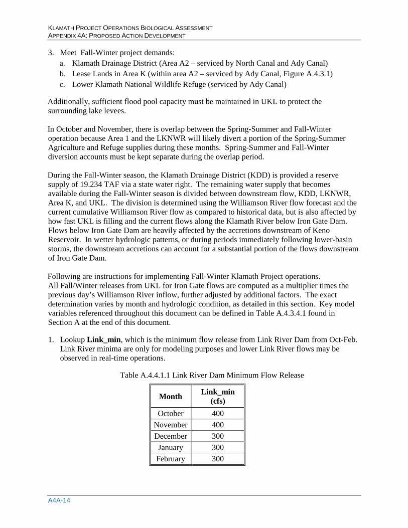
1. Lookup Link_min, which is the minimum flow release from Link River Dam from Oct-Feb. Link River minima are only for modeling purposes and lower Link River flows may be observed in real-time operations.
Table A.4.4.1.1 Link River Dam Minimum Flow Release
Month Link_min (cfs)
October 400 November 400 December 300 January 300 February 300
KLAMATH PROJECT OPERATIONS BIOLOGICAL ASSESSMENT APPENDIX 4A: PROPOSED ACTION DEVELOPMENT
A4A-15
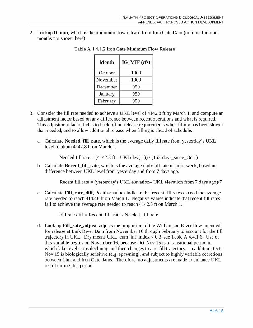
2. Lookup IGmin, which is the minimum flow release from Iron Gate Dam (minima for other months not shown here):
Table A.4.4.1.2 Iron Gate Minimum Flow Release
Month IG_MIF (cfs)
October 1000 November 1000 December 950 January 950 February 950
3. Consider the fill rate needed to achieve a UKL level of 4142.8 ft by March 1, and compute an adjustment factor based on any difference between recent operations and what is required. This adjustment factor helps to back off on release requirements when filling has been slower than needed, and to allow additional release when filling is ahead of schedule.
a. Calculate Needed_fill_rate, which is the average daily fill rate from yesterday’s UKL level to attain 4142.8 ft on March 1.
Needed fill rate = (4142.8 ft – UKLelev(-1)) / (152-days_since_Oct1)
b. Calculate Recent_fill_rate, which is the average daily fill rate of prior week, based on difference between UKL level from yesterday and from 7 days ago.
Recent fill rate = (yesterday’s UKL elevation– UKL elevation from 7 days ago)/7
c. Calculate Fill_rate_diff, Positive values indicate that recent fill rates exceed the average rate needed to reach 4142.8 ft on March 1. Negative values indicate that recent fill rates fail to achieve the average rate needed to reach 4142.8 ft on March 1.
Fill rate diff = Recent_fill_rate - Needed_fill_rate
d. Look up Fill_rate_adjust, adjusts the proportion of the Williamson River flow intended for release at Link River Dam from November 16 through February to account for the fill trajectory in UKL. Dry means UKL_cum_inf_index < 0.3, see Table A.4.4.1.6. Use of this variable begins on November 16, because Oct-Nov 15 is a transitional period in which lake level stops declining and then changes to a re-fill trajectory. In addition, Oct-Nov 15 is biologically sensitive (e.g. spawning), and subject to highly variable accretions between Link and Iron Gate dams. Therefore, no adjustments are made to enhance UKL re-fill during this period.
KLAMATH PROJECT OPERATIONS BIOLOGICAL ASSESSMENT APPENDIX 4A: PROPOSED ACTION DEVELOPMENT
A4A-16
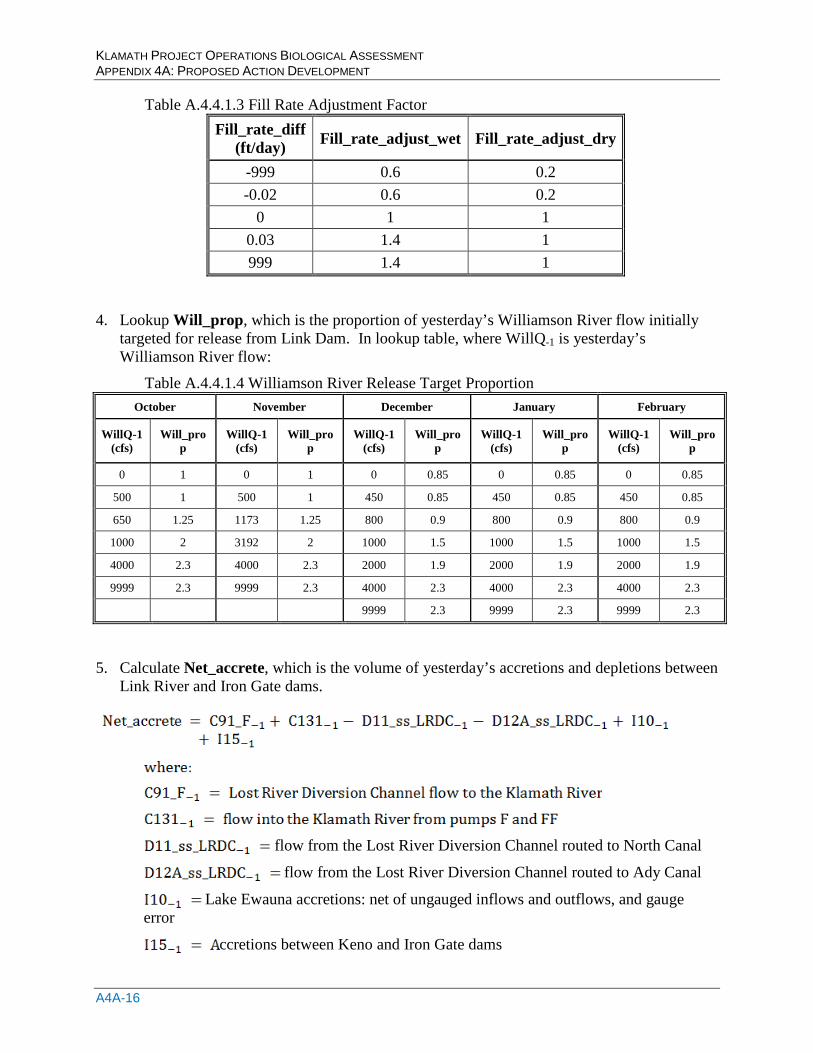
Table A.4.4.1.3 Fill Rate Adjustment Factor Fill_rate_diff
(ft/day) Fill_rate_adjust_wet Fill_rate_adjust_dry
-999 0.6 0.2 -0.02 0.6 0.2
0 1 1 0.03 1.4 1 999 1.4 1
4. Lookup Will_prop, which is the proportion of yesterday’s Williamson River flow initially targeted for release from Link Dam. In lookup table, where WillQ-1 is yesterday’s Williamson River flow:
Table A.4.4.1.4 Williamson River Release Target Proportion October November December January February
WillQ-1 (cfs)
Will_prop
WillQ-1 (cfs)
Will_prop
WillQ-1 (cfs)
Will_prop
WillQ-1 (cfs)
Will_prop
WillQ-1 (cfs)
Will_prop
0 1 0 1 0 0.85 0 0.85 0 0.85
500 1 500 1 450 0.85 450 0.85 450 0.85
650 1.25 1173 1.25 800 0.9 800 0.9 800 0.9
1000 2 3192 2 1000 1.5 1000 1.5 1000 1.5
4000 2.3 4000 2.3 2000 1.9 2000 1.9 2000 1.9
9999 2.3 9999 2.3 4000 2.3 4000 2.3 4000 2.3
9999 2.3 9999 2.3 9999 2.3
5. Calculate Net_accrete, which is the volume of yesterday’s accretions and depletions between Link River and Iron Gate dams.
flow from the Lost River Diversion Channel routed to North Canal
flow from the Lost River Diversion Channel routed to Ady Canal
Lake Ewauna accretions: net of ungauged inflows and outflows, and gauge error
ccretions between Keno and Iron Gate dams
KLAMATH PROJECT OPERATIONS BIOLOGICAL ASSESSMENT APPENDIX 4A: PROPOSED ACTION DEVELOPMENT
A4A-17
the previous day
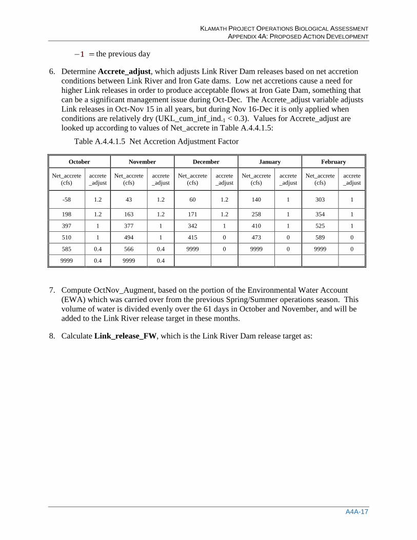
6. Determine Accrete_adjust, which adjusts Link River Dam releases based on net accretion conditions between Link River and Iron Gate dams. Low net accretions cause a need for higher Link releases in order to produce acceptable flows at Iron Gate Dam, something that can be a significant management issue during Oct-Dec. The Accrete_adjust variable adjusts Link releases in Oct-Nov 15 in all years, but during Nov 16-Dec it is only applied when conditions are relatively dry (UKL_cum_inf_ind-1 < 0.3). Values for Accrete_adjust are looked up according to values of Net_accrete in Table A.4.4.1.5:
Table A.4.4.1.5 Net Accretion Adjustment Factor
October November December January February
Net_accrete (cfs)
accrete _adjust
Net_accrete (cfs)
accrete _adjust
Net_accrete (cfs)
accrete _adjust
Net_accrete (cfs)
accrete _adjust
Net_accrete (cfs)
accrete _adjust
-58 1.2 43 1.2 60 1.2 140 1 303 1
198 1.2 163 1.2 171 1.2 258 1 354 1
397 1 377 1 342 1 410 1 525 1
510 1 494 1 415 0 473 0 589 0
585 0.4 566 0.4 9999 0 9999 0 9999 0
9999 0.4 9999 0.4
7. Compute OctNov_Augment, based on the portion of the Environmental Water Account (EWA) which was carried over from the previous Spring/Summer operations season. This volume of water is divided evenly over the 61 days in October and November, and will be added to the Link River release target in these months.
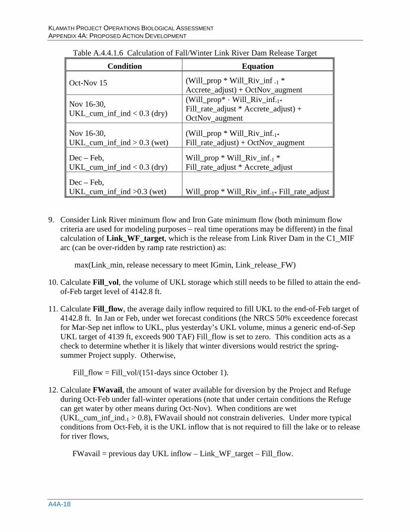
8. Calculate Link_release_FW, which is the Link River Dam release target as:
KLAMATH PROJECT OPERATIONS BIOLOGICAL ASSESSMENT APPENDIX 4A: PROPOSED ACTION DEVELOPMENT
A4A-18
Table A.4.4.1.6 Calculation of Fall/Winter Link River Dam Release Target
Condition Equation
Oct-Nov 15 (Will_prop * Will_Riv_inf -1 * Accrete_adjust) + OctNov_augment
Nov 16-30, UKL_cum_inf_ind < 0.3 (dry)
(Will_prop* · Will_Riv_inf-1* Fill_rate_adjust * Accrete_adjust) + OctNov_augment
Nov 16-30, UKL_cum_inf_ind > 0.3 (wet)
(Will_prop * Will_Riv_inf-1* Fill_rate_adjust) + OctNov_augment
Dec – Feb, UKL_cum_inf_ind < 0.3 (dry)
Will_prop * Will_Riv_inf-1 * Fill_rate_adjust * Accrete_adjust
Dec – Feb, UKL_cum_inf_ind >0.3 (wet) Will_prop * Will_Riv_inf-1* Fill_rate_adjust
9. Consider Link River minimum flow and Iron Gate minimum flow (both minimum flow criteria are used for modeling purposes – real time operations may be different) in the final calculation of Link_WF_target, which is the release from Link River Dam in the C1_MIF arc (can be over-ridden by ramp rate restriction) as:
max(Link_min, release necessary to meet IGmin, Link_release_FW)
10. Calculate Fill_vol, the volume of UKL storage which still needs to be filled to attain the end-of-Feb target level of 4142.8 ft.
11. Calculate Fill_flow, the average daily inflow required to fill UKL to the end-of-Feb target of 4142.8 ft. In Jan or Feb, under wet forecast conditions (the NRCS 50% exceedence forecast for Mar-Sep net inflow to UKL, plus yesterday’s UKL volume, minus a generic end-of-Sep UKL target of 4139 ft, exceeds 900 TAF) Fill_flow is set to zero. This condition acts as a check to determine whether it is likely that winter diversions would restrict the spring-summer Project supply. Otherwise,
Fill_flow = Fill_vol/(151-days since October 1).
12. Calculate FWavail, the amount of water available for diversion by the Project and Refuge during Oct-Feb under fall-winter operations (note that under certain conditions the Refuge can get water by other means during Oct-Nov). When conditions are wet (UKL_cum_inf_ind-1 > 0.8), FWavail should not constrain deliveries. Under more typical conditions from Oct-Feb, it is the UKL inflow that is not required to fill the lake or to release for river flows,
FWavail = previous day UKL inflow – Link_WF_target – Fill_flow.
KLAMATH PROJECT OPERATIONS BIOLOGICAL ASSESSMENT APPENDIX 4A: PROPOSED ACTION DEVELOPMENT
A4A-19
A.4.4.2 Spring-Summer Operations The Klamath Project irrigation season runs from March 1st through September 30th, however irrigation often continues into October and November depending on the year type, crops planted and the hydrologic conditions at the end of each water year. The previous section described the Fall/Winter operations which are the first half of each water year. This section describes the second half of each water year, which covers the irrigation season. The irrigation season operations are controlled by defining the available project supply, which is computed from storage in Upper Klamath Lake, forecasted March-September inflow, and target carryover storage. Based on this supply, a portion is made available to the River and Project supply is computed based on multiple parameters. Any UKL inflow that is not delivered or released for flow will remain in UKL as storage. All water which leaves UKL through either Link River Dam or the A Canal is accounted for against one of these two identified volumes; this includes flood control releases. The Lower Klamath National Wildlife Refuge can receive a portion of the project supply or other delivery from UKL. Details for these operations are included in the sections below.
Project Water Supply and Environmental Water Account for Klamath River Flows Both volumes are calculated on March 1st and April 1st with updates on May 1st and June 1st. The March and April processes divide up the UKL supply to help the irrigators and River managers plan out the spring and summer seasons. The May and June processes manage the change in supply by adjusting the volumes. The steps for determining the Project water supply and the Environmental Water Account (EWA) are below. Key model variables referenced throughout this section can be found in Table A.4.3.4.1 at the end of this Appendix 4A-1.
1. Calculate UKLsupply - The UKL supply is updated on the 1st of each month for March
through June using the most current forecasted net inflow, the end of February storage and the end of September target. This formula is as follows (all values in TAF):
UKLsupply = [End of February UKL Storage] + [50% exceedance forecast UKL inflow for March through September] – [End of September UKL Storage Target] a. The end of February UKL storage is simply the storage in UKL as determined on the last
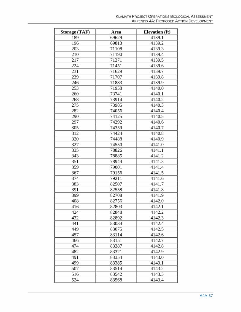
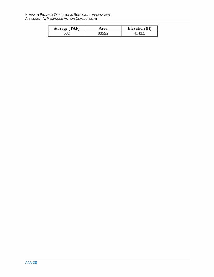
day of February. This is determined using the UKL weighted mean average elevation as determined by the United States Geological Survey (USGS) for that date along with the elevation-storage table included as Table A.4.4.2.1 found at the end of this Appendix.
b. The forecasted UKL inflow for March through September changes each month from March through June. The formulas used for this variable (called Mar50vol in the model code) are as follows: i. March = [March 1st 50% exceedance probability forecast for UKL net inflows for
March through September] ii. April = [April 1st 50% exceedance probability forecast for UKL net inflows for April
through September] + [Actual Inflows that Occurred in March] iii. May = [May 1st 50% exceedance probability forecast for UKL net inflows for May
through September] + [Actual Inflows that Occurred in March] + [Actual Inflows that Occurred in April]
KLAMATH PROJECT OPERATIONS BIOLOGICAL ASSESSMENT APPENDIX 4A: PROPOSED ACTION DEVELOPMENT
A4A-20
iv. June = [June 1st 50% exceedance probability forecast for UKL net inflows for June through September] + [Actual Inflows that Occurred in March] + [Actual Inflows that Occurred in April] + [Actual Inflows that Occurred in May]
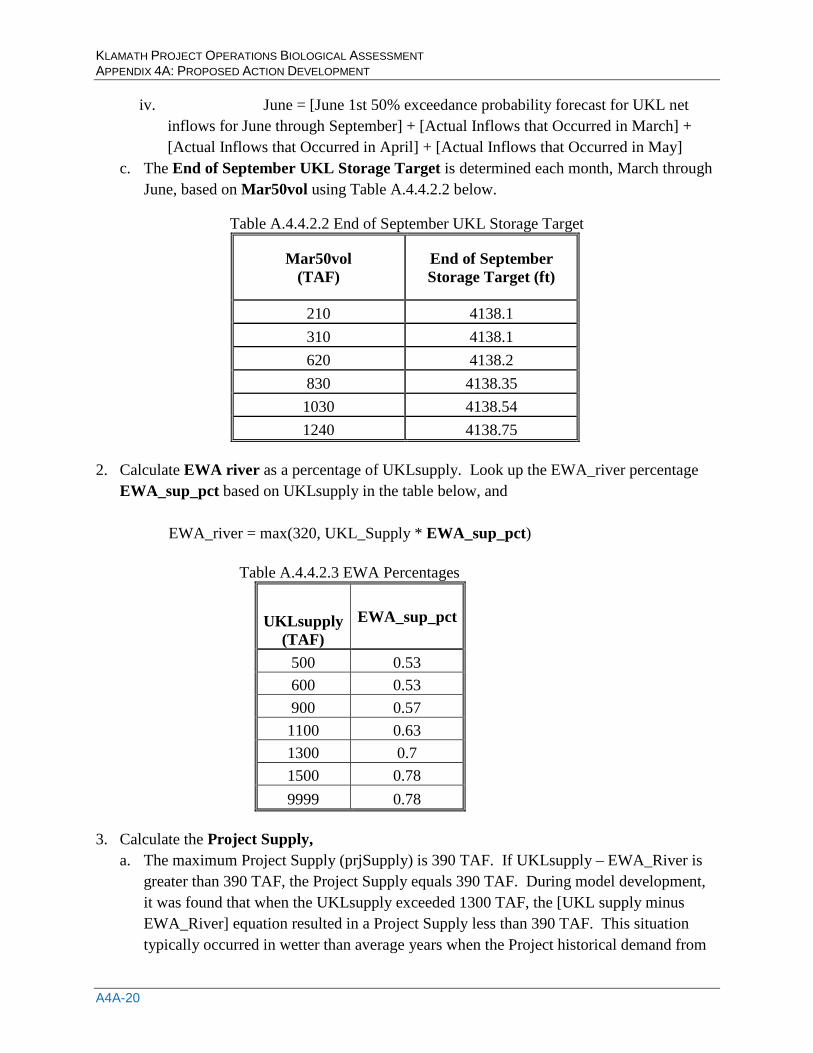
c. The End of September UKL Storage Target is determined each month, March through June, based on Mar50vol using Table A.4.4.2.2 below.
Table A.4.4.2.2 End of September UKL Storage Target
Mar50vol (TAF)
End of September Storage Target (ft)
210 4138.1 310 4138.1 620 4138.2 830 4138.35 1030 4138.54 1240 4138.75
2. Calculate EWA river as a percentage of UKLsupply. Look up the EWA_river percentage
EWA_sup_pct based on UKLsupply in the table below, and EWA_river = max(320, UKL_Supply * EWA_sup_pct)
Table A.4.4.2.3 EWA Percentages
UKLsupply (TAF)
EWA_sup_pct
500 0.53 600 0.53 900 0.57 1100 0.63 1300 0.7 1500 0.78 9999 0.78
3. Calculate the Project Supply,
a. The maximum Project Supply (prjSupply) is 390 TAF. If UKLsupply – EWA_River is greater than 390 TAF, the Project Supply equals 390 TAF. During model development, it was found that when the UKLsupply exceeded 1300 TAF, the [UKL supply minus EWA_River] equation resulted in a Project Supply less than 390 TAF. This situation typically occurred in wetter than average years when the Project historical demand from
KLAMATH PROJECT OPERATIONS BIOLOGICAL ASSESSMENT APPENDIX 4A: PROPOSED ACTION DEVELOPMENT
A4A-21
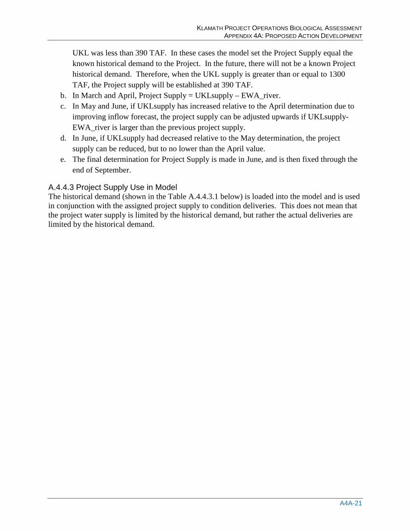
UKL was less than 390 TAF. In these cases the model set the Project Supply equal the known historical demand to the Project. In the future, there will not be a known Project historical demand. Therefore, when the UKL supply is greater than or equal to 1300 TAF, the Project supply will be established at 390 TAF.
b. In March and April, Project Supply = UKLsupply – EWA_river. c. In May and June, if UKLsupply has increased relative to the April determination due to
improving inflow forecast, the project supply can be adjusted upwards if UKLsupply-EWA_river is larger than the previous project supply.
d. In June, if UKLsupply had decreased relative to the May determination, the project supply can be reduced, but to no lower than the April value.
e. The final determination for Project Supply is made in June, and is then fixed through the end of September.
A.4.4.3 Project Supply Use in Model The historical demand (shown in the Table A.4.4.3.1 below) is loaded into the model and is used in conjunction with the assigned project supply to condition deliveries. This does not mean that the project water supply is limited by the historical demand, but rather the actual deliveries are limited by the historical demand.
KLAMATH PROJECT OPERATIONS BIOLOGICAL ASSESSMENT APPENDIX 4A: PROPOSED ACTION DEVELOPMENT
A4A-22
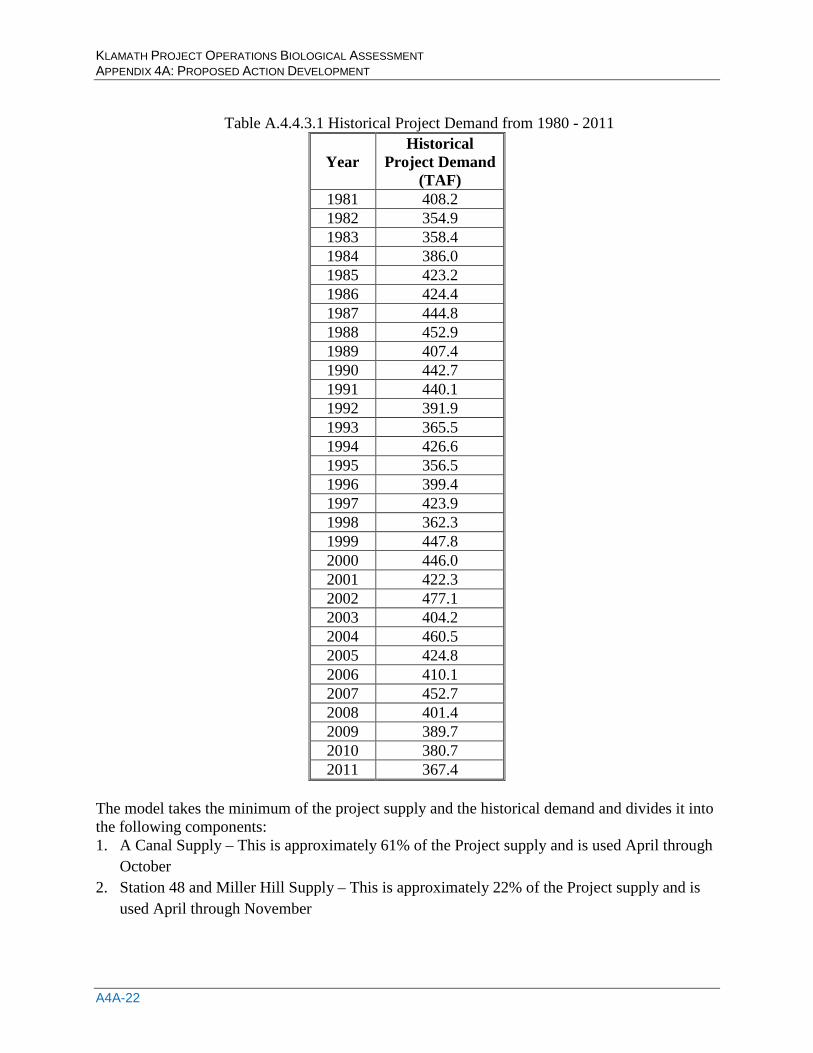
Table A.4.4.3.1 Historical Project Demand from 1980 - 2011
Year
Historical Project Demand
(TAF) 1981 408.2 1982 354.9 1983 358.4 1984 386.0 1985 423.2 1986 424.4 1987 444.8 1988 452.9 1989 407.4 1990 442.7 1991 440.1 1992 391.9 1993 365.5 1994 426.6 1995 356.5 1996 399.4 1997 423.9 1998 362.3 1999 447.8 2000 446.0 2001 422.3 2002 477.1 2003 404.2 2004 460.5 2005 424.8 2006 410.1 2007 452.7 2008 401.4 2009 389.7 2010 380.7 2011 367.4
The model takes the minimum of the project supply and the historical demand and divides it into the following components: 1. A Canal Supply – This is approximately 61% of the Project supply and is used April through
October 2. Station 48 and Miller Hill Supply – This is approximately 22% of the Project supply and is
used April through November
KLAMATH PROJECT OPERATIONS BIOLOGICAL ASSESSMENT APPENDIX 4A: PROPOSED ACTION DEVELOPMENT
A4A-23
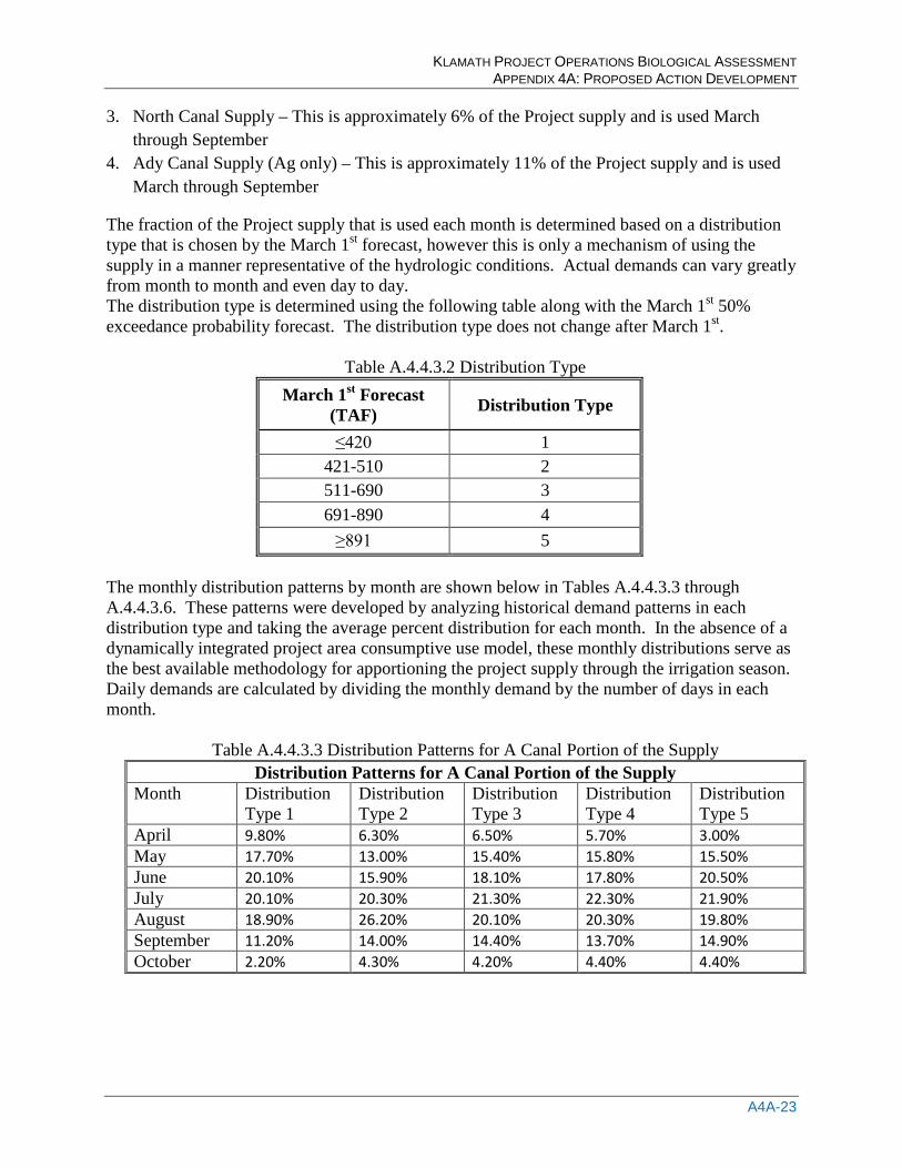
3. North Canal Supply – This is approximately 6% of the Project supply and is used March through September
4. Ady Canal Supply (Ag only) – This is approximately 11% of the Project supply and is used March through September
The fraction of the Project supply that is used each month is determined based on a distribution type that is chosen by the March 1st forecast, however this is only a mechanism of using the supply in a manner representative of the hydrologic conditions. Actual demands can vary greatly from month to month and even day to day. The distribution type is determined using the following table along with the March 1st 50% exceedance probability forecast. The distribution type does not change after March 1st.
Table A.4.4.3.2 Distribution Type
March 1st Forecast (TAF) Distribution Type
≤420 1 421-510 2 511-690 3 691-890 4 ≥891 5
The monthly distribution patterns by month are shown below in Tables A.4.4.3.3 through A.4.4.3.6. These patterns were developed by analyzing historical demand patterns in each distribution type and taking the average percent distribution for each month. In the absence of a dynamically integrated project area consumptive use model, these monthly distributions serve as the best available methodology for apportioning the project supply through the irrigation season. Daily demands are calculated by dividing the monthly demand by the number of days in each month.
Table A.4.4.3.3 Distribution Patterns for A Canal Portion of the Supply
Distribution Patterns for A Canal Portion of the Supply Month
Distribution Type 1
Distribution Type 2
Distribution Type 3
Distribution Type 4
Distribution Type 5
April 9.80% 6.30% 6.50% 5.70% 3.00% May 17.70% 13.00% 15.40% 15.80% 15.50% June 20.10% 15.90% 18.10% 17.80% 20.50% July 20.10% 20.30% 21.30% 22.30% 21.90% August 18.90% 26.20% 20.10% 20.30% 19.80% September 11.20% 14.00% 14.40% 13.70% 14.90% October 2.20% 4.30% 4.20% 4.40% 4.40%
KLAMATH PROJECT OPERATIONS BIOLOGICAL ASSESSMENT APPENDIX 4A: PROPOSED ACTION DEVELOPMENT
A4A-24
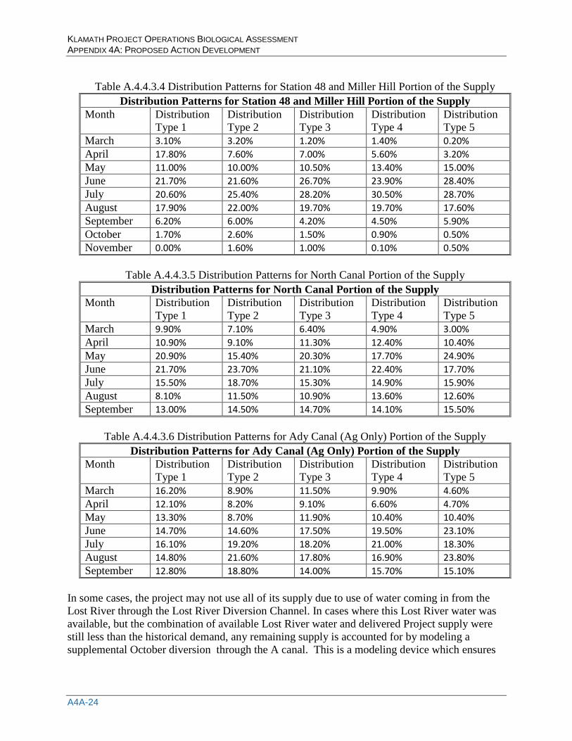
Table A.4.4.3.4 Distribution Patterns for Station 48 and Miller Hill Portion of the Supply
Distribution Patterns for Station 48 and Miller Hill Portion of the Supply Month
Distribution Type 1
Distribution Type 2
Distribution Type 3
Distribution Type 4
Distribution Type 5
March 3.10% 3.20% 1.20% 1.40% 0.20% April 17.80% 7.60% 7.00% 5.60% 3.20% May 11.00% 10.00% 10.50% 13.40% 15.00% June 21.70% 21.60% 26.70% 23.90% 28.40% July 20.60% 25.40% 28.20% 30.50% 28.70% August 17.90% 22.00% 19.70% 19.70% 17.60% September 6.20% 6.00% 4.20% 4.50% 5.90% October 1.70% 2.60% 1.50% 0.90% 0.50% November 0.00% 1.60% 1.00% 0.10% 0.50%
Table A.4.4.3.5 Distribution Patterns for North Canal Portion of the Supply Distribution Patterns for North Canal Portion of the Supply
Month
Distribution Type 1
Distribution Type 2
Distribution Type 3
Distribution Type 4
Distribution Type 5
March 9.90% 7.10% 6.40% 4.90% 3.00% April 10.90% 9.10% 11.30% 12.40% 10.40% May 20.90% 15.40% 20.30% 17.70% 24.90% June 21.70% 23.70% 21.10% 22.40% 17.70% July 15.50% 18.70% 15.30% 14.90% 15.90% August 8.10% 11.50% 10.90% 13.60% 12.60% September 13.00% 14.50% 14.70% 14.10% 15.50%
Table A.4.4.3.6 Distribution Patterns for Ady Canal (Ag Only) Portion of the Supply Distribution Patterns for Ady Canal (Ag Only) Portion of the Supply
Month
Distribution Type 1
Distribution Type 2
Distribution Type 3
Distribution Type 4
Distribution Type 5
March 16.20% 8.90% 11.50% 9.90% 4.60% April 12.10% 8.20% 9.10% 6.60% 4.70% May 13.30% 8.70% 11.90% 10.40% 10.40% June 14.70% 14.60% 17.50% 19.50% 23.10% July 16.10% 19.20% 18.20% 21.00% 18.30% August 14.80% 21.60% 17.80% 16.90% 23.80% September 12.80% 18.80% 14.00% 15.70% 15.10%
In some cases, the project may not use all of its supply due to use of water coming in from the Lost River through the Lost River Diversion Channel. In cases where this Lost River water was available, but the combination of available Lost River water and delivered Project supply were still less than the historical demand, any remaining supply is accounted for by modeling a supplemental October diversion through the A canal. This is a modeling device which ensures
KLAMATH PROJECT OPERATIONS BIOLOGICAL ASSESSMENT APPENDIX 4A: PROPOSED ACTION DEVELOPMENT
A4A-25
that the model does not cause simulated shortages to the project when the supply would not otherwise be fully used.
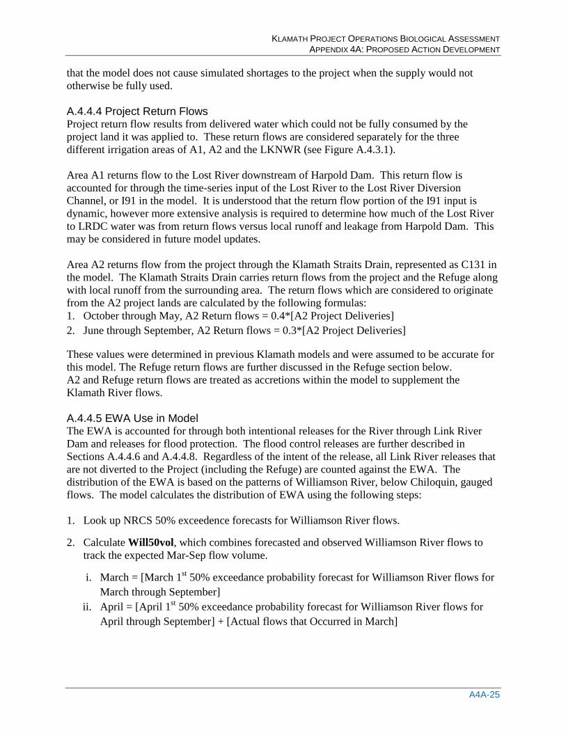
A.4.4.4 Project Return Flows Project return flow results from delivered water which could not be fully consumed by the project land it was applied to. These return flows are considered separately for the three different irrigation areas of A1, A2 and the LKNWR (see Figure A.4.3.1). Area A1 returns flow to the Lost River downstream of Harpold Dam. This return flow is accounted for through the time-series input of the Lost River to the Lost River Diversion Channel, or I91 in the model. It is understood that the return flow portion of the I91 input is dynamic, however more extensive analysis is required to determine how much of the Lost River to LRDC water was from return flows versus local runoff and leakage from Harpold Dam. This may be considered in future model updates. Area A2 returns flow from the project through the Klamath Straits Drain, represented as C131 in the model. The Klamath Straits Drain carries return flows from the project and the Refuge along with local runoff from the surrounding area. The return flows which are considered to originate from the A2 project lands are calculated by the following formulas: 1. October through May, A2 Return flows = 0.4*[A2 Project Deliveries] 2. June through September, A2 Return flows = 0.3*[A2 Project Deliveries]
These values were determined in previous Klamath models and were assumed to be accurate for this model. The Refuge return flows are further discussed in the Refuge section below. A2 and Refuge return flows are treated as accretions within the model to supplement the Klamath River flows. A.4.4.5 EWA Use in Model The EWA is accounted for through both intentional releases for the River through Link River Dam and releases for flood protection. The flood control releases are further described in Sections A.4.4.6 and A.4.4.8. Regardless of the intent of the release, all Link River releases that are not diverted to the Project (including the Refuge) are counted against the EWA. The distribution of the EWA is based on the patterns of Williamson River, below Chiloquin, gauged flows. The model calculates the distribution of EWA using the following steps: 1. Look up NRCS 50% exceedence forecasts for Williamson River flows.
2. Calculate Will50vol, which combines forecasted and observed Williamson River flows to track the expected Mar-Sep flow volume.
i. March = [March 1st 50% exceedance probability forecast for Williamson River flows for March through September]
ii. April = [April 1st 50% exceedance probability forecast for Williamson River flows for April through September] + [Actual flows that Occurred in March]
KLAMATH PROJECT OPERATIONS BIOLOGICAL ASSESSMENT APPENDIX 4A: PROPOSED ACTION DEVELOPMENT
A4A-26
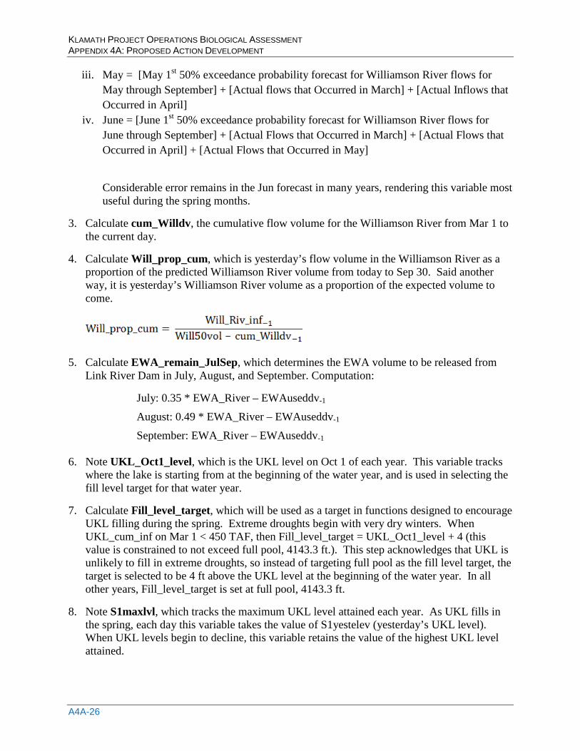
iii. May = [May 1st 50% exceedance probability forecast for Williamson River flows for May through September] + [Actual flows that Occurred in March] + [Actual Inflows that Occurred in April]
iv. June = [June 1st 50% exceedance probability forecast for Williamson River flows for June through September] + [Actual Flows that Occurred in March] + [Actual Flows that Occurred in April] + [Actual Flows that Occurred in May]
Considerable error remains in the Jun forecast in many years, rendering this variable most useful during the spring months.
3. Calculate cum_Willdv, the cumulative flow volume for the Williamson River from Mar 1 to the current day.
4. Calculate Will_prop_cum, which is yesterday’s flow volume in the Williamson River as a proportion of the predicted Williamson River volume from today to Sep 30. Said another way, it is yesterday’s Williamson River volume as a proportion of the expected volume to come.
5. Calculate EWA_remain_JulSep, which determines the EWA volume to be released from Link River Dam in July, August, and September. Computation:
July: 0.35 * EWA_River – EWAuseddv-1
August: 0.49 * EWA_River – EWAuseddv-1
September: EWA_River – EWAuseddv-1
6. Note UKL_Oct1_level, which is the UKL level on Oct 1 of each year. This variable tracks where the lake is starting from at the beginning of the water year, and is used in selecting the fill level target for that water year.
7. Calculate Fill_level_target, which will be used as a target in functions designed to encourage UKL filling during the spring. Extreme droughts begin with very dry winters. When UKL_cum_inf on Mar 1 < 450 TAF, then Fill_level_target = UKL_Oct1_level + 4 (this value is constrained to not exceed full pool, 4143.3 ft.). This step acknowledges that UKL is unlikely to fill in extreme droughts, so instead of targeting full pool as the fill level target, the target is selected to be 4 ft above the UKL level at the beginning of the water year. In all other years, Fill_level_target is set at full pool, 4143.3 ft.
8. Note S1maxlvl, which tracks the maximum UKL level attained each year. As UKL fills in the spring, each day this variable takes the value of S1yestelev (yesterday’s UKL level). When UKL levels begin to decline, this variable retains the value of the highest UKL level attained.
KLAMATH PROJECT OPERATIONS BIOLOGICAL ASSESSMENT APPENDIX 4A: PROPOSED ACTION DEVELOPMENT
A4A-27
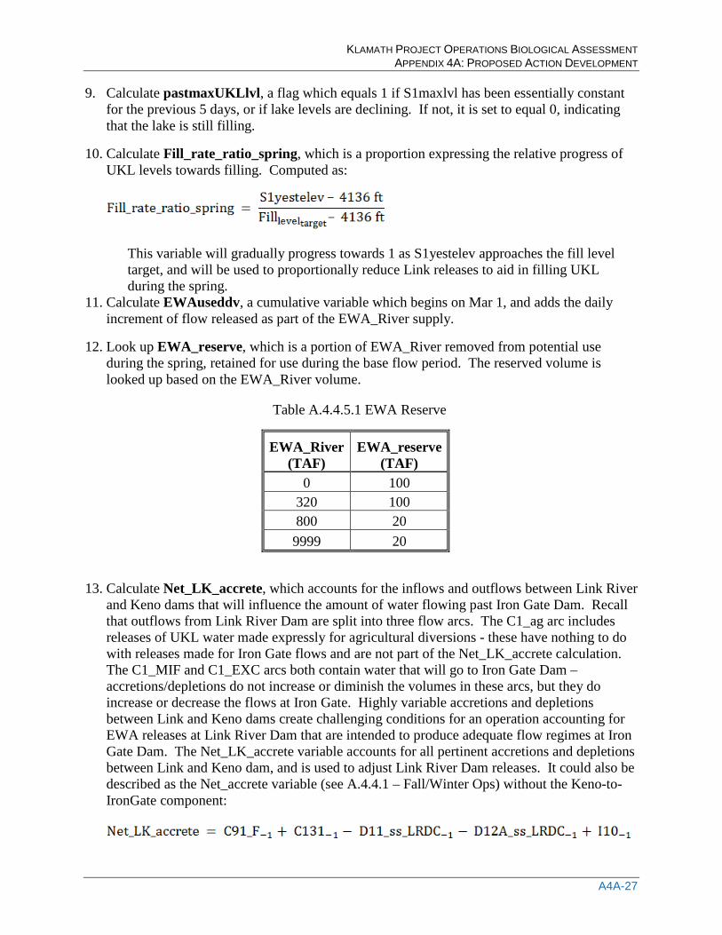
9. Calculate pastmaxUKLlvl, a flag which equals 1 if S1maxlvl has been essentially constant for the previous 5 days, or if lake levels are declining. If not, it is set to equal 0, indicating that the lake is still filling.
10. Calculate Fill_rate_ratio_spring, which is a proportion expressing the relative progress of UKL levels towards filling. Computed as:
This variable will gradually progress towards 1 as S1yestelev approaches the fill level target, and will be used to proportionally reduce Link releases to aid in filling UKL during the spring.
11. Calculate EWAuseddv, a cumulative variable which begins on Mar 1, and adds the daily increment of flow released as part of the EWA_River supply.
12. Look up EWA_reserve, which is a portion of EWA_River removed from potential use during the spring, retained for use during the base flow period. The reserved volume is looked up based on the EWA_River volume.
Table A.4.4.5.1 EWA Reserve
EWA_River (TAF)
EWA_reserve (TAF)
0 100 320 100 800 20 9999 20
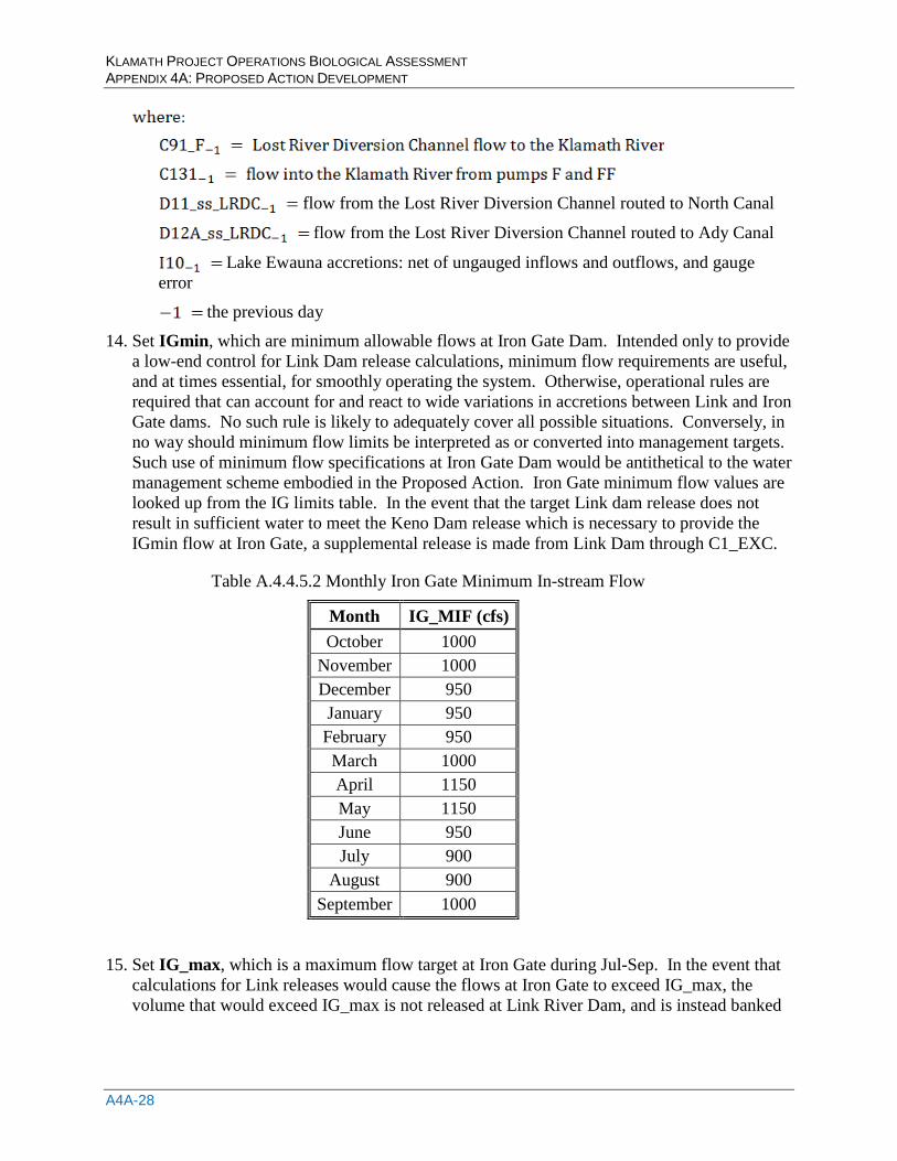
13. Calculate Net_LK_accrete, which accounts for the inflows and outflows between Link River and Keno dams that will influence the amount of water flowing past Iron Gate Dam. Recall that outflows from Link River Dam are split into three flow arcs. The C1_ag arc includes releases of UKL water made expressly for agricultural diversions - these have nothing to do with releases made for Iron Gate flows and are not part of the Net_LK_accrete calculation. The C1_MIF and C1_EXC arcs both contain water that will go to Iron Gate Dam – accretions/depletions do not increase or diminish the volumes in these arcs, but they do increase or decrease the flows at Iron Gate. Highly variable accretions and depletions between Link and Keno dams create challenging conditions for an operation accounting for EWA releases at Link River Dam that are intended to produce adequate flow regimes at Iron Gate Dam. The Net_LK_accrete variable accounts for all pertinent accretions and depletions between Link and Keno dam, and is used to adjust Link River Dam releases. It could also be described as the Net_accrete variable (see A.4.4.1 – Fall/Winter Ops) without the Keno-to-IronGate component:
KLAMATH PROJECT OPERATIONS BIOLOGICAL ASSESSMENT APPENDIX 4A: PROPOSED ACTION DEVELOPMENT
A4A-28
flow from the Lost River Diversion Channel routed to North Canal
flow from the Lost River Diversion Channel routed to Ady Canal
Lake Ewauna accretions: net of ungauged inflows and outflows, and gauge error
the previous day
14. Set IGmin, which are minimum allowable flows at Iron Gate Dam. Intended only to provide a low-end control for Link Dam release calculations, minimum flow requirements are useful, and at times essential, for smoothly operating the system. Otherwise, operational rules are required that can account for and react to wide variations in accretions between Link and Iron Gate dams. No such rule is likely to adequately cover all possible situations. Conversely, in no way should minimum flow limits be interpreted as or converted into management targets. Such use of minimum flow specifications at Iron Gate Dam would be antithetical to the water management scheme embodied in the Proposed Action. Iron Gate minimum flow values are looked up from the IG limits table. In the event that the target Link dam release does not result in sufficient water to meet the Keno Dam release which is necessary to provide the IGmin flow at Iron Gate, a supplemental release is made from Link Dam through C1_EXC.
Table A.4.4.5.2 Monthly Iron Gate Minimum In-stream Flow
Month IG_MIF (cfs) October 1000
November 1000 December 950 January 950 February 950 March 1000 April 1150 May 1150 June 950 July 900
August 900 September 1000
15. Set IG_max, which is a maximum flow target at Iron Gate during Jul-Sep. In the event that calculations for Link releases would cause the flows at Iron Gate to exceed IG_max, the volume that would exceed IG_max is not released at Link River Dam, and is instead banked
KLAMATH PROJECT OPERATIONS BIOLOGICAL ASSESSMENT APPENDIX 4A: PROPOSED ACTION DEVELOPMENT
A4A-29
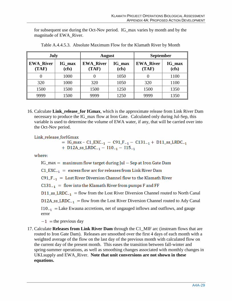
for subsequent use during the Oct-Nov period. IG_max varies by month and by the magnitude of EWA_River.
Table A.4.4.5.3. Absolute Maximum Flow for the Klamath River by Month
July August September
EWA_River (TAF)
IG_max (cfs)
EWA_River (TAF)
IG_max (cfs)
EWA_River (TAF)
IG_max (cfs)
0 1000 0 1050 0 1100 320 1000 320 1050 320 1100 1500 1500 1500 1250 1500 1350 9999 1500 9999 1250 9999 1350
16. Calculate Link_release_for IGmax, which is the approximate release from Link River Dam necessary to produce the IG_max flow at Iron Gate. Calculated only during Jul-Sep, this variable is used to determine the volume of EWA water, if any, that will be carried over into the Oct-Nov period.
IG_max
flow from the Lost River Diversion Channel routed to North Canal
flow from the Lost River Diversion Channel routed to Ady Canal
Lake Ewauna accretions, net of ungauged inflows and outflows, and gauge error
the previous day
17. Calculate Releases from Link River Dam through the C1_MIF arc (instream flows that are routed to Iron Gate Dam). Releases are smoothed over the first 4 days of each month with a weighted average of the flow on the last day of the previous month with calculated flow on the current day of the present month. This eases the transition between fall-winter and spring-summer operations, as well as smoothing changes associated with monthly changes in UKLsupply and EWA_River. Note that unit conversions are not shown in these equations.
KLAMATH PROJECT OPERATIONS BIOLOGICAL ASSESSMENT APPENDIX 4A: PROPOSED ACTION DEVELOPMENT
A4A-30
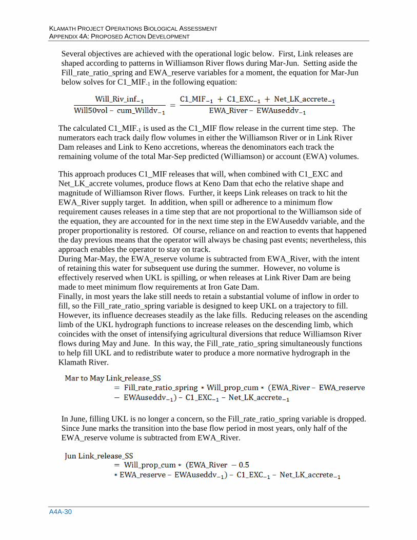
Several objectives are achieved with the operational logic below. First, Link releases are shaped according to patterns in Williamson River flows during Mar-Jun. Setting aside the Fill_rate_ratio_spring and EWA_reserve variables for a moment, the equation for Mar-Jun below solves for C1_MIF-1 in the following equation:
The calculated C1_MIF-1 is used as the C1_MIF flow release in the current time step. The numerators each track daily flow volumes in either the Williamson River or in Link River Dam releases and Link to Keno accretions, whereas the denominators each track the remaining volume of the total Mar-Sep predicted (Williamson) or account (EWA) volumes.
This approach produces C1_MIF releases that will, when combined with C1_EXC and Net_LK_accrete volumes, produce flows at Keno Dam that echo the relative shape and magnitude of Williamson River flows. Further, it keeps Link releases on track to hit the EWA_River supply target. In addition, when spill or adherence to a minimum flow requirement causes releases in a time step that are not proportional to the Williamson side of the equation, they are accounted for in the next time step in the EWAuseddv variable, and the proper proportionality is restored. Of course, reliance on and reaction to events that happened the day previous means that the operator will always be chasing past events; nevertheless, this approach enables the operator to stay on track. During Mar-May, the EWA_reserve volume is subtracted from EWA_River, with the intent of retaining this water for subsequent use during the summer. However, no volume is effectively reserved when UKL is spilling, or when releases at Link River Dam are being made to meet minimum flow requirements at Iron Gate Dam. Finally, in most years the lake still needs to retain a substantial volume of inflow in order to fill, so the Fill_rate_ratio_spring variable is designed to keep UKL on a trajectory to fill. However, its influence decreases steadily as the lake fills. Reducing releases on the ascending limb of the UKL hydrograph functions to increase releases on the descending limb, which coincides with the onset of intensifying agricultural diversions that reduce Williamson River flows during May and June. In this way, the Fill_rate_ratio_spring simultaneously functions to help fill UKL and to redistribute water to produce a more normative hydrograph in the Klamath River.
In June, filling UKL is no longer a concern, so the Fill_rate_ratio_spring variable is dropped. Since June marks the transition into the base flow period in most years, only half of the EWA_reserve volume is subtracted from EWA_River.
KLAMATH PROJECT OPERATIONS BIOLOGICAL ASSESSMENT APPENDIX 4A: PROPOSED ACTION DEVELOPMENT
A4A-31
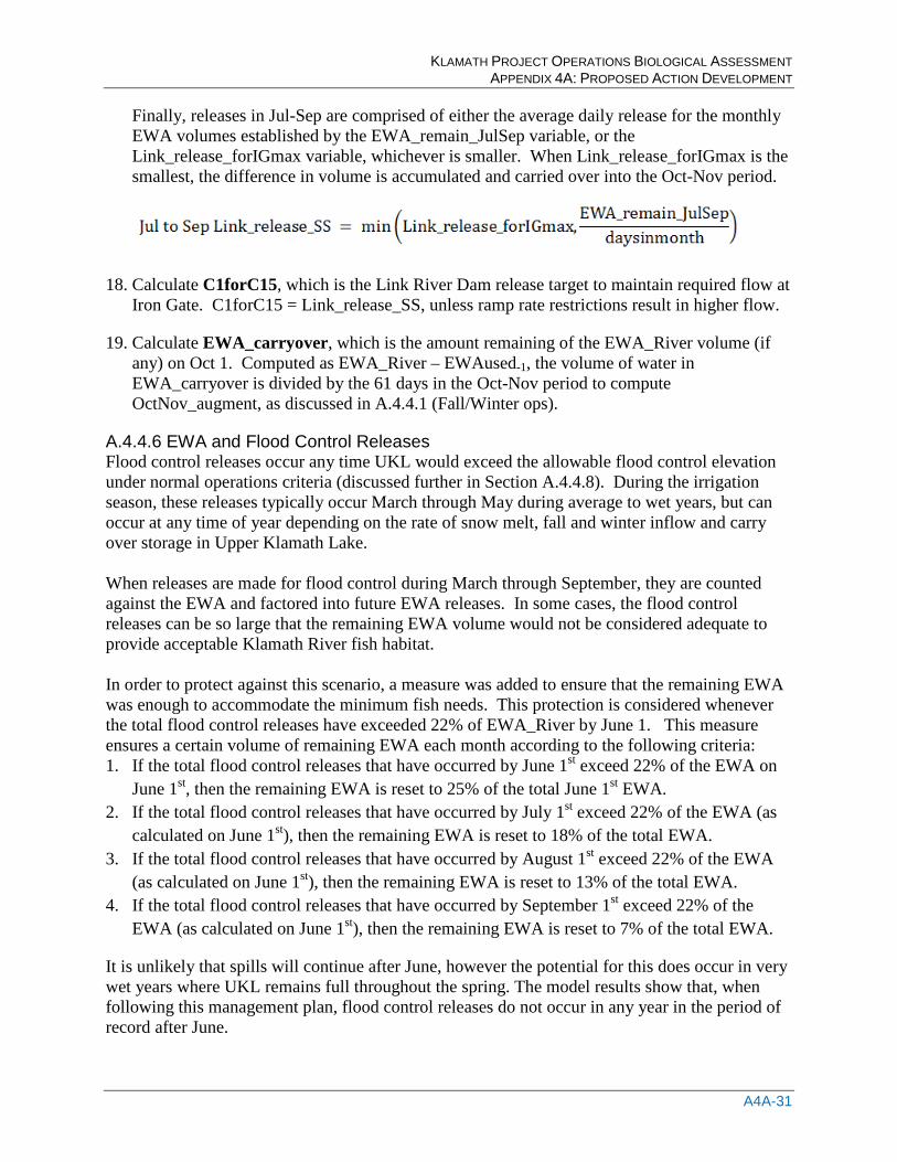
Finally, releases in Jul-Sep are comprised of either the average daily release for the monthly EWA volumes established by the EWA_remain_JulSep variable, or the Link_release_forIGmax variable, whichever is smaller. When Link_release_forIGmax is the smallest, the difference in volume is accumulated and carried over into the Oct-Nov period.
18. Calculate C1forC15, which is the Link River Dam release target to maintain required flow at Iron Gate. C1forC15 = Link_release_SS, unless ramp rate restrictions result in higher flow.
19. Calculate EWA_carryover, which is the amount remaining of the EWA_River volume (if any) on Oct 1. Computed as EWA_River – EWAused-1, the volume of water in EWA_carryover is divided by the 61 days in the Oct-Nov period to compute OctNov_augment, as discussed in A.4.4.1 (Fall/Winter ops).
A.4.4.6 EWA and Flood Control Releases Flood control releases occur any time UKL would exceed the allowable flood control elevation under normal operations criteria (discussed further in Section A.4.4.8). During the irrigation season, these releases typically occur March through May during average to wet years, but can occur at any time of year depending on the rate of snow melt, fall and winter inflow and carry over storage in Upper Klamath Lake. When releases are made for flood control during March through September, they are counted against the EWA and factored into future EWA releases. In some cases, the flood control releases can be so large that the remaining EWA volume would not be considered adequate to provide acceptable Klamath River fish habitat. In order to protect against this scenario, a measure was added to ensure that the remaining EWA was enough to accommodate the minimum fish needs. This protection is considered whenever the total flood control releases have exceeded 22% of EWA_River by June 1. This measure ensures a certain volume of remaining EWA each month according to the following criteria: 1. If the total flood control releases that have occurred by June 1st exceed 22% of the EWA on
June 1st, then the remaining EWA is reset to 25% of the total June 1st EWA. 2. If the total flood control releases that have occurred by July 1st exceed 22% of the EWA (as
calculated on June 1st), then the remaining EWA is reset to 18% of the total EWA. 3. If the total flood control releases that have occurred by August 1st exceed 22% of the EWA
(as calculated on June 1st), then the remaining EWA is reset to 13% of the total EWA. 4. If the total flood control releases that have occurred by September 1st exceed 22% of the
EWA (as calculated on June 1st), then the remaining EWA is reset to 7% of the total EWA.
It is unlikely that spills will continue after June, however the potential for this does occur in very wet years where UKL remains full throughout the spring. The model results show that, when following this management plan, flood control releases do not occur in any year in the period of record after June.
KLAMATH PROJECT OPERATIONS BIOLOGICAL ASSESSMENT APPENDIX 4A: PROPOSED ACTION DEVELOPMENT
A4A-32
A.4.4.7 Refuge Operation There is no automatic project supply assigned to the refuge. Refuge delivery targets are determined by a combination of project supply and UKL storage conditions. The refuge can receive non-project water or a portion of the project supply, but not both. 1. The refuge has no target delivery March-May. 2. The refuge has no target delivery in June-July if the project supply is below 390 TAF. 3. In June through November, if the project has full supply (390 TAF) and if the UKL elevation
is above the Threshold level denoted in Table A.4.4.7.1, the delivery target is set according to the monthly demand (also Table A.4.4.7.1). These deliveries are not counted against project supply, and they can be served from local accretions or UKL storage releases.
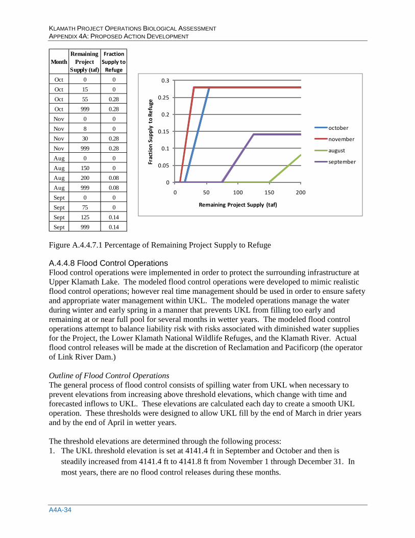
4. In August through November, if either the project supply is lower than 390 TAF or the UKL elevation is below the Table A.4.4.7.1 Threshold level, a portion of the remaining project supply can be reserved for refuge delivery, calculated by the following process. a. Calculate the remaining project supply on the first day of each month August-November. b. Define the fraction of the remaining project supply that is to be made available to the
Refuge, AugNovRfgFactor, according to the table and plot shown in Figure A.4.4.7.1 c. Determine the lake level adjustment threshold
i. Aug-Sep – interpolate the UKL adjustment threshold using the Spring/Summer day counter (counts from March 1) and the associated thresholds in Table A.4.4.7.2
ii. Oct-Nov – interpolate the UKL adjustment threshold using the water year day counter (counts from October 1) and the associated thresholds in Table A.4.4.7.2
d. Calculate the lake level adjustment UKL_rfg_adjust, which reduces the project refuge supply when the UKL level gets too far below the threshold. If the UKL level is at or above the adjustment threshold, there is no adjustment, so UKL_rfg_adjust is 1.0. If the UKL level is .3 feet below the adjustment threshold, the project refuge supply gets turned off by setting UKL_rfg_adjust to 0.0. For UKL levels between the threshold and .3 feet below the threshold, the factor is interpolated between 1 and 0. UKL_rfg_adjust = 1.0 – min(0.3, max(0.0, UKL_rfg_adjust_thresh – UKL_level(-1)))/0.3
e. Calculate the RfgTgt_vol (water volume available to be delivered to the refuge in the current month) as: RfrTgt_vol = Remaining Project Supply * AugNovRfgFactor * UKL_rfg_adjust

KLAMATH PROJECT OPERATIONS BIOLOGICAL ASSESSMENT APPENDIX 4A: PROPOSED ACTION DEVELOPMENT
A4A-33
Table A.4.4.7.1 Monthly Refuge Demand and UKL Elevation Thresholds Which Condition Refuge Delivery
Table A.4.4.7.2 Upper Klamath Lake and Refuge Adjustment Threshold
Month Refuge
Demand (TAF)
UKL Threshold
(ft) January 15.18 4139.0 February 11.53 4139.5 March 7.93 4140.0 April 7.93 4140.5 May 7.93 4141.5 June 0 4142.5 July 3.63 4143.0
August 5.28 4143.0 September 5.94 4142.5
October 6.93 4141.5 November 5.94 4140.5 December 17.16 4139.5
SSdaynum UKL_level (ft) (Aug-Sep)
154 4140.0 184 4139.1 214 4138.6
daynum UKL_level (ft) (Oct-Nov)
1 4138.6 31 4138.6 61 4138.9
KLAMATH PROJECT OPERATIONS BIOLOGICAL ASSESSMENT APPENDIX 4A: PROPOSED ACTION DEVELOPMENT
A4A-34
MonthRemaining
Project Supply (taf)
Fraction Supply to
Refuge
Oct 0 0Oct 15 0Oct 55 0.28Oct 999 0.28Nov 0 0Nov 8 0Nov 30 0.28Nov 999 0.28Aug 0 0Aug 150 0Aug 200 0.08Aug 999 0.08Sept 0 0Sept 75 0Sept 125 0.14Sept 999 0.14
0
0.05
0.1
0.15
0.2
0.25
0.3
0 50 100 150 200
Frac
tion
Supp
ly t
o Re
fuge
Remaining Project Supply (taf)
october
november
august
september
Figure A.4.4.7.1 Percentage of Remaining Project Supply to Refuge A.4.4.8 Flood Control Operations Flood control operations were implemented in order to protect the surrounding infrastructure at Upper Klamath Lake. The modeled flood control operations were developed to mimic realistic flood control operations; however real time management should be used in order to ensure safety and appropriate water management within UKL. The modeled operations manage the water during winter and early spring in a manner that prevents UKL from filling too early and remaining at or near full pool for several months in wetter years. The modeled flood control operations attempt to balance liability risk with risks associated with diminished water supplies for the Project, the Lower Klamath National Wildlife Refuges, and the Klamath River. Actual flood control releases will be made at the discretion of Reclamation and Pacificorp (the operator of Link River Dam.) Outline of Flood Control Operations The general process of flood control consists of spilling water from UKL when necessary to prevent elevations from increasing above threshold elevations, which change with time and forecasted inflows to UKL. These elevations are calculated each day to create a smooth UKL operation. These thresholds were designed to allow UKL fill by the end of March in drier years and by the end of April in wetter years. The threshold elevations are determined through the following process: 1. The UKL threshold elevation is set at 4141.4 ft in September and October and then is
steadily increased from 4141.4 ft to 4141.8 ft from November 1 through December 31. In most years, there are no flood control releases during these months.
KLAMATH PROJECT OPERATIONS BIOLOGICAL ASSESSMENT APPENDIX 4A: PROPOSED ACTION DEVELOPMENT
A4A-35
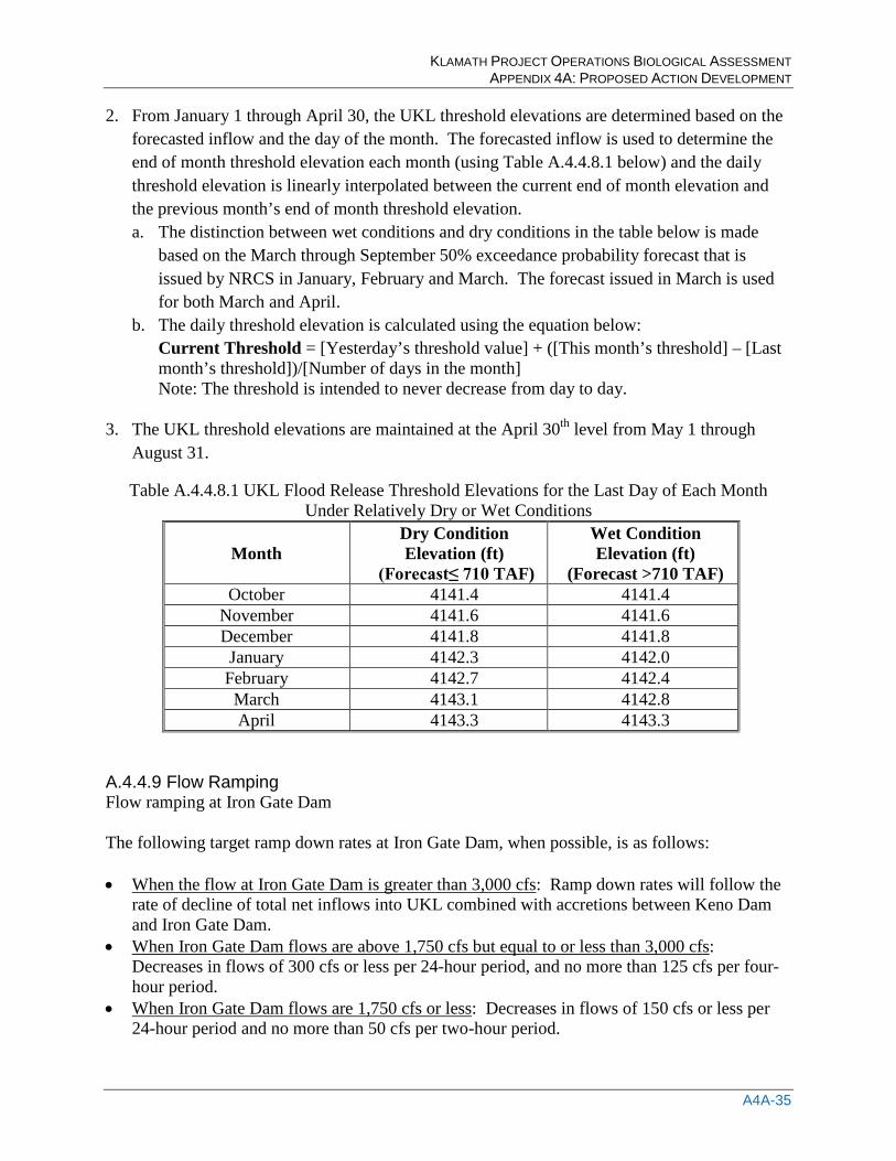
2. From January 1 through April 30, the UKL threshold elevations are determined based on the forecasted inflow and the day of the month. The forecasted inflow is used to determine the end of month threshold elevation each month (using Table A.4.4.8.1 below) and the daily threshold elevation is linearly interpolated between the current end of month elevation and the previous month’s end of month threshold elevation. a. The distinction between wet conditions and dry conditions in the table below is made
based on the March through September 50% exceedance probability forecast that is issued by NRCS in January, February and March. The forecast issued in March is used for both March and April.
b. The daily threshold elevation is calculated using the equation below: Current Threshold = [Yesterday’s threshold value] + ([This month’s threshold] – [Last month’s threshold])/[Number of days in the month] Note: The threshold is intended to never decrease from day to day.
3. The UKL threshold elevations are maintained at the April 30th level from May 1 through
August 31.
Table A.4.4.8.1 UKL Flood Release Threshold Elevations for the Last Day of Each Month Under Relatively Dry or Wet Conditions
Month
Dry Condition Elevation (ft)
(Forecast≤ 710 TAF)
Wet Condition Elevation (ft)
(Forecast >710 TAF) October 4141.4 4141.4
November 4141.6 4141.6 December 4141.8 4141.8 January 4142.3 4142.0 February 4142.7 4142.4 March 4143.1 4142.8 April 4143.3 4143.3
A.4.4.9 Flow Ramping Flow ramping at Iron Gate Dam The following target ramp down rates at Iron Gate Dam, when possible, is as follows: • When the flow at Iron Gate Dam is greater than 3,000 cfs: Ramp down rates will follow the
rate of decline of total net inflows into UKL combined with accretions between Keno Dam and Iron Gate Dam.
• When Iron Gate Dam flows are above 1,750 cfs but equal to or less than 3,000 cfs: Decreases in flows of 300 cfs or less per 24-hour period, and no more than 125 cfs per four-hour period.
• When Iron Gate Dam flows are 1,750 cfs or less: Decreases in flows of 150 cfs or less per 24-hour period and no more than 50 cfs per two-hour period.

KLAMATH PROJECT OPERATIONS BIOLOGICAL ASSESSMENT APPENDIX 4A: PROPOSED ACTION DEVELOPMENT
A4A-36
Upward ramping was not restricted. The WRIMS model does not include operations of storage capacity within the PacifiCorp facilities. Therefore the model is only able to adjust Link River Dam releases to attempt to comply with the ramping rate restrictions assumed. Link River Dam releases cannot necessarily be adjusted to comply with the ramping rate restrictions if unregulated flows are present at Link River Dam or Iron Gate Dam. The WRIMS model recognizes when these unregulated flow conditions exist and, under those conditions, does not attempt to comply with the ramping rate restrictions.
Table A.4.4.2.1 Elevation Storage-Area Storage (TAF) Area Elevation (ft)
0 46229 4136.0 5 47243 4136.1 9 48458 4136.2 14 49674 4136.3 19 50991 4136.4 25 52309 4136.5 30 53628 4136.6 35 54947 4136.7 41 56068 4136.8 47 56990 4136.9 52 58012 4137.0 58 58935 4137.1 64 59860 4137.2 70 60585 4137.3 76 61310 4137.4 82 61937 4137.5 89 62600 4137.6 95 63263 4137.7 101 63927 4137.8 108 64592 4137.9 114 65157 4138.0 121 65842 4138.1 127 66407 4138.2 134 66973 4138.3 141 67339 4138.4 148 67610 4138.5 154 67800 4138.6 161 68089 4138.7 168 68377 4138.8 175 68664 4138.9 182 68950 4139.0
KLAMATH PROJECT OPERATIONS BIOLOGICAL ASSESSMENT APPENDIX 4A: PROPOSED ACTION DEVELOPMENT
A4A-37
Storage (TAF) Area Elevation (ft) 189 69629 4139.1 196 69813 4139.2 203 71108 4139.3 210 71190 4139.4 217 71371 4139.5 224 71451 4139.6 231 71629 4139.7 239 71707 4139.8 246 71883 4139.9 253 71958 4140.0 260 73741 4140.1 268 73914 4140.2 275 73985 4140.3 282 74056 4140.4 290 74125 4140.5 297 74292 4140.6 305 74359 4140.7 312 74424 4140.8 320 74488 4140.9 327 74550 4141.0 335 78826 4141.1 343 78885 4141.2 351 78944 4141.3 359 79001 4141.4 367 79156 4141.5 374 79211 4141.6 383 82507 4141.7 391 82558 4141.8 399 82708 4141.9 408 82756 4142.0 416 82803 4142.1 424 82848 4142.2 432 82892 4142.3 441 83034 4142.4 449 83075 4142.5 457 83114 4142.6 466 83151 4142.7 474 83287 4142.8 482 83321 4142.9 491 83354 4143.0 499 83385 4143.1 507 83514 4143.2 516 83542 4143.3 524 83568 4143.4
KLAMATH PROJECT OPERATIONS BIOLOGICAL ASSESSMENT APPENDIX 4A: PROPOSED ACTION DEVELOPMENT
A4A-38
Storage (TAF) Area Elevation (ft) 532 83592 4143.5

KLAMATH PROJECT OPERATIONS BIOLOGICAL ASSESSMENT APPENDIX 4A: PROPOSED ACTION DEVELOPMENT
A4A-39
Section A: Key Model Variables

KLAMATH PROJECT OPERATIONS BIOLOGICAL ASSESSMENT APPENDIX 4A: PROPOSED ACTION DEVELOPMENT
A4A-40
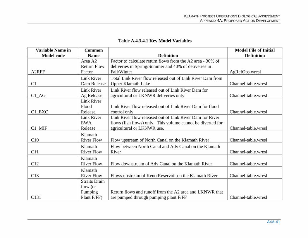
KLAMATH PROJECT OPERATIONS BIOLOGICAL ASSESSMENT APPENDIX 4A: PROPOSED ACTION DEVELOPMENT
A4A-41
Table A.4.3.4.1 Key Model Variables
Variable Name in Model code
Common Name Definition
Model File of Initial Definition
A2RFF
Area A2 Return Flow Factor
Factor to calculate return flows from the A2 area - 30% of deliveries in Spring/Summer and 40% of deliveries in Fall/Winter AgRefOps.wresl
C1 Link River Dam Release
Total Link River flow released out of Link River Dam from Upper Klamath Lake Channel-table.wresl
C1_AG Link River Ag Release
Link River flow released out of Link River Dam for agricultural or LKNWR deliveries only Channel-table.wresl
C1_EXC
Link River Flood Release
Link River flow released out of Link River Dam for flood control only Channel-table.wresl
C1_MIF
Link River EWA Release
Link River flow released out of Link River Dam for River flows (fish flows) only. This volume cannot be diverted for agricultural or LKNWR use. Channel-table.wresl
C10 Klamath River Flow Flow upstream of North Canal on the Klamath River Channel-table.wresl
C11 Klamath River Flow
Flow between North Canal and Ady Canal on the Klamath River Channel-table.wresl
C12 Klamath River Flow Flow downstream of Ady Canal on the Klamath River Channel-table.wresl
C13 Klamath River Flow Flows upstream of Keno Reservoir on the Klamath River Channel-table.wresl
C131
Straits Drain flow (or Pumping Plant F/FF)
Return flows and runoff from the A2 area and LKNWR that are pumped through pumping plant F/FF Channel-table.wresl
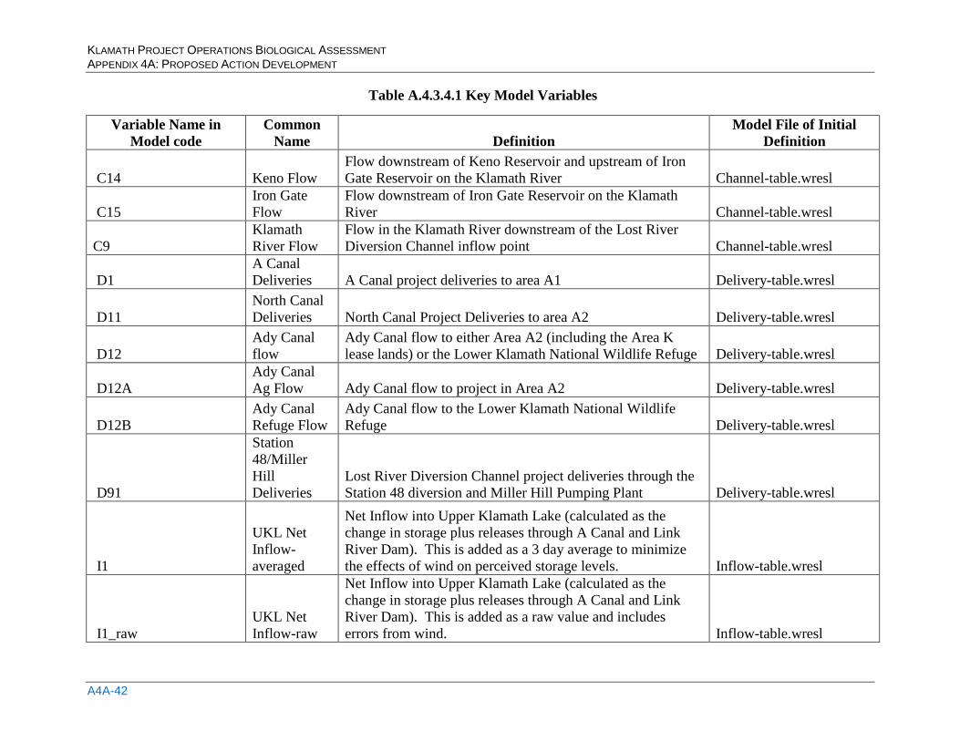
KLAMATH PROJECT OPERATIONS BIOLOGICAL ASSESSMENT APPENDIX 4A: PROPOSED ACTION DEVELOPMENT
A4A-42
Table A.4.3.4.1 Key Model Variables
Variable Name in Model code
Common Name Definition
Model File of Initial Definition
C14 Keno Flow Flow downstream of Keno Reservoir and upstream of Iron Gate Reservoir on the Klamath River Channel-table.wresl
C15 Iron Gate Flow
Flow downstream of Iron Gate Reservoir on the Klamath River Channel-table.wresl
C9 Klamath River Flow
Flow in the Klamath River downstream of the Lost River Diversion Channel inflow point Channel-table.wresl
D1 A Canal Deliveries A Canal project deliveries to area A1 Delivery-table.wresl
D11 North Canal Deliveries North Canal Project Deliveries to area A2 Delivery-table.wresl
D12 Ady Canal flow
Ady Canal flow to either Area A2 (including the Area K lease lands) or the Lower Klamath National Wildlife Refuge Delivery-table.wresl
D12A Ady Canal Ag Flow Ady Canal flow to project in Area A2 Delivery-table.wresl
D12B Ady Canal Refuge Flow
Ady Canal flow to the Lower Klamath National Wildlife Refuge Delivery-table.wresl
D91
Station 48/Miller Hill Deliveries
Lost River Diversion Channel project deliveries through the Station 48 diversion and Miller Hill Pumping Plant Delivery-table.wresl
I1
UKL Net Inflow-averaged
Net Inflow into Upper Klamath Lake (calculated as the change in storage plus releases through A Canal and Link River Dam). This is added as a 3 day average to minimize the effects of wind on perceived storage levels. Inflow-table.wresl
I1_raw UKL Net Inflow-raw
Net Inflow into Upper Klamath Lake (calculated as the change in storage plus releases through A Canal and Link River Dam). This is added as a raw value and includes errors from wind. Inflow-table.wresl
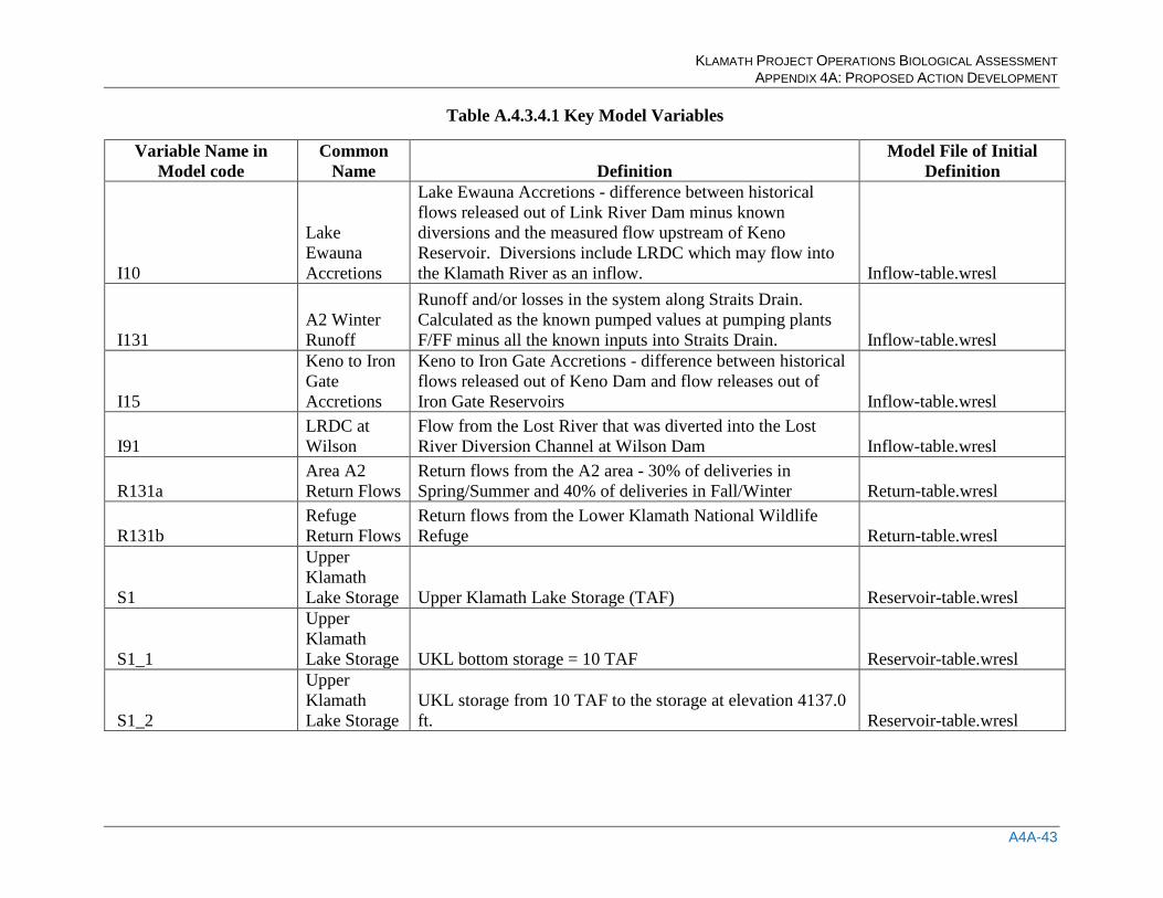
KLAMATH PROJECT OPERATIONS BIOLOGICAL ASSESSMENT APPENDIX 4A: PROPOSED ACTION DEVELOPMENT
A4A-43
Table A.4.3.4.1 Key Model Variables
Variable Name in Model code
Common Name Definition
Model File of Initial Definition
I10
Lake Ewauna Accretions
Lake Ewauna Accretions - difference between historical flows released out of Link River Dam minus known diversions and the measured flow upstream of Keno Reservoir. Diversions include LRDC which may flow into the Klamath River as an inflow. Inflow-table.wresl
I131 A2 Winter Runoff
Runoff and/or losses in the system along Straits Drain. Calculated as the known pumped values at pumping plants F/FF minus all the known inputs into Straits Drain. Inflow-table.wresl
I15
Keno to Iron Gate Accretions
Keno to Iron Gate Accretions - difference between historical flows released out of Keno Dam and flow releases out of Iron Gate Reservoirs Inflow-table.wresl
I91 LRDC at Wilson
Flow from the Lost River that was diverted into the Lost River Diversion Channel at Wilson Dam Inflow-table.wresl
R131a Area A2 Return Flows
Return flows from the A2 area - 30% of deliveries in Spring/Summer and 40% of deliveries in Fall/Winter Return-table.wresl
R131b Refuge Return Flows
Return flows from the Lower Klamath National Wildlife Refuge Return-table.wresl
S1
Upper Klamath Lake Storage Upper Klamath Lake Storage (TAF) Reservoir-table.wresl
S1_1
Upper Klamath Lake Storage UKL bottom storage = 10 TAF Reservoir-table.wresl
S1_2
Upper Klamath Lake Storage
UKL storage from 10 TAF to the storage at elevation 4137.0 ft. Reservoir-table.wresl
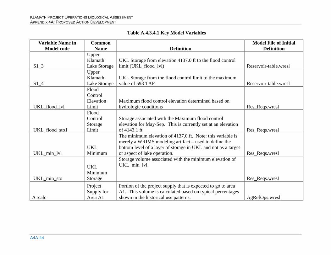
KLAMATH PROJECT OPERATIONS BIOLOGICAL ASSESSMENT APPENDIX 4A: PROPOSED ACTION DEVELOPMENT
A4A-44
Table A.4.3.4.1 Key Model Variables
Variable Name in Model code
Common Name Definition
Model File of Initial Definition
S1_3
Upper Klamath Lake Storage
UKL Storage from elevation 4137.0 ft to the flood control limit (UKL_flood_lvl) Reservoir-table.wresl
S1_4
Upper Klamath Lake Storage
UKL Storage from the flood control limit to the maximum value of 593 TAF Reservoir-table.wresl
UKL_flood_lvl
Flood Control Elevation Limit
Maximum flood control elevation determined based on hydrologic conditions Res_Reqs.wresl
UKL_flood_sto1
Flood Control Storage Limit
Storage associated with the Maximum flood control elevation for May-Sep. This is currently set at an elevation of 4143.1 ft. Res_Reqs.wresl
UKL_min_lvl UKL Minimum
The minimum elevation of 4137.0 ft. Note: this variable is merely a WRIMS modeling artifact – used to define the bottom level of a layer of storage in UKL and not as a target or aspect of lake operation. Res_Reqs.wresl
UKL_min_sto
UKL Minimum Storage
Storage volume associated with the minimum elevation of UKL_min_lvl.
Res_Reqs.wresl
A1calc
Project Supply for Area A1
Portion of the project supply that is expected to go to area A1. This volume is calculated based on typical percentages shown in the historical use patterns. AgRefOps.wresl
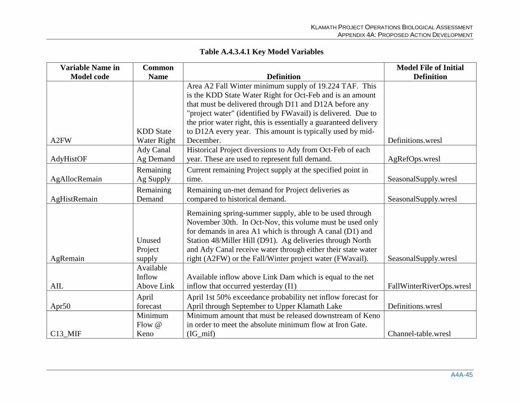
KLAMATH PROJECT OPERATIONS BIOLOGICAL ASSESSMENT APPENDIX 4A: PROPOSED ACTION DEVELOPMENT
A4A-45
Table A.4.3.4.1 Key Model Variables
Variable Name in Model code
Common Name Definition
Model File of Initial Definition
A2FW KDD State Water Right
Area A2 Fall Winter minimum supply of 19.224 TAF. This is the KDD State Water Right for Oct-Feb and is an amount that must be delivered through D11 and D12A before any "project water" (identified by FWavail) is delivered. Due to the prior water right, this is essentially a guaranteed delivery to D12A every year. This amount is typically used by mid-December. Definitions.wresl
AdyHistOF Ady Canal Ag Demand
Historical Project diversions to Ady from Oct-Feb of each year. These are used to represent full demand. AgRefOps.wresl
AgAllocRemain Remaining Ag Supply
Current remaining Project supply at the specified point in time. SeasonalSupply.wresl
AgHistRemain Remaining Demand
Remaining un-met demand for Project deliveries as compared to historical demand. SeasonalSupply.wresl
AgRemain
Unused Project supply
Remaining spring-summer supply, able to be used through November 30th. In Oct-Nov, this volume must be used only for demands in area A1 which is through A canal (D1) and Station 48/Miller Hill (D91). Ag deliveries through North and Ady Canal receive water through either their state water right (A2FW) or the Fall/Winter project water (FWavail). SeasonalSupply.wresl
AIL
Available Inflow Above Link
Available inflow above Link Dam which is equal to the net inflow that occurred yesterday (I1) FallWinterRiverOps.wresl
Apr50 April forecast
April 1st 50% exceedance probability net inflow forecast for April through September to Upper Klamath Lake Definitions.wresl
C13_MIF
Minimum Flow @ Keno
Minimum amount that must be released downstream of Keno in order to meet the absolute minimum flow at Iron Gate. (IG_mif) Channel-table.wresl
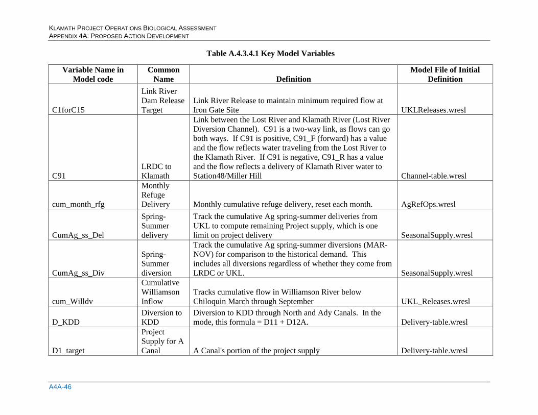
KLAMATH PROJECT OPERATIONS BIOLOGICAL ASSESSMENT APPENDIX 4A: PROPOSED ACTION DEVELOPMENT
A4A-46
Table A.4.3.4.1 Key Model Variables
Variable Name in Model code
Common Name Definition
Model File of Initial Definition
C1forC15
Link River Dam Release Target
Link River Release to maintain minimum required flow at Iron Gate Site UKLReleases.wresl
C91 LRDC to Klamath
Link between the Lost River and Klamath River (Lost River Diversion Channel). C91 is a two-way link, as flows can go both ways. If C91 is positive, C91_F (forward) has a value and the flow reflects water traveling from the Lost River to the Klamath River. If C91 is negative, C91_R has a value and the flow reflects a delivery of Klamath River water to Station48/Miller Hill Channel-table.wresl
cum_month_rfg
Monthly Refuge Delivery Monthly cumulative refuge delivery, reset each month. AgRefOps.wresl
CumAg_ss_Del
Spring-Summer delivery
Track the cumulative Ag spring-summer deliveries from UKL to compute remaining Project supply, which is one limit on project delivery SeasonalSupply.wresl
CumAg_ss_Div
Spring-Summer diversion
Track the cumulative Ag spring-summer diversions (MAR-NOV) for comparison to the historical demand. This includes all diversions regardless of whether they come from LRDC or UKL. SeasonalSupply.wresl
cum_Willdv
Cumulative Williamson Inflow
Tracks cumulative flow in Williamson River below Chiloquin March through September UKL_Releases.wresl
D_KDD Diversion to KDD
Diversion to KDD through North and Ady Canals. In the mode, this formula = D11 + D12A. Delivery-table.wresl
D1_target
Project Supply for A Canal A Canal's portion of the project supply Delivery-table.wresl
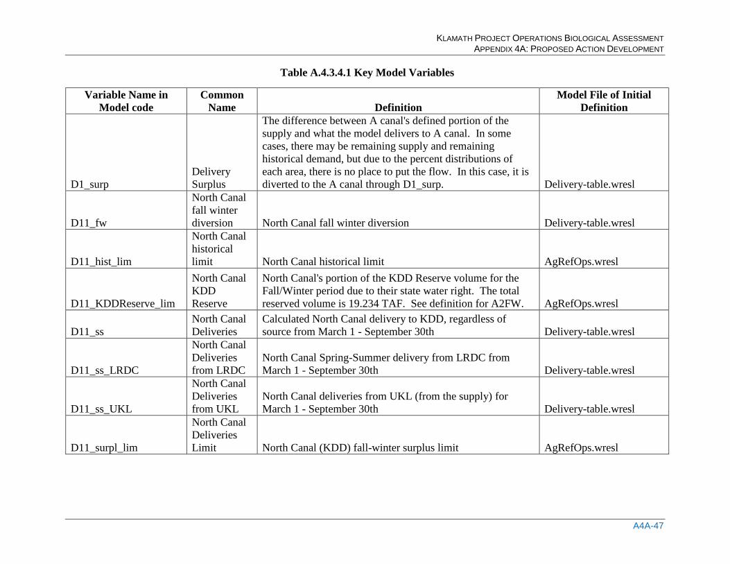
KLAMATH PROJECT OPERATIONS BIOLOGICAL ASSESSMENT APPENDIX 4A: PROPOSED ACTION DEVELOPMENT
A4A-47
Table A.4.3.4.1 Key Model Variables
Variable Name in Model code
Common Name Definition
Model File of Initial Definition
D1_surp Delivery Surplus
The difference between A canal's defined portion of the supply and what the model delivers to A canal. In some cases, there may be remaining supply and remaining historical demand, but due to the percent distributions of each area, there is no place to put the flow. In this case, it is diverted to the A canal through D1_surp. Delivery-table.wresl
D11_fw
North Canal fall winter diversion North Canal fall winter diversion Delivery-table.wresl
D11_hist_lim
North Canal historical limit North Canal historical limit AgRefOps.wresl
D11_KDDReserve_lim
North Canal KDD Reserve
North Canal's portion of the KDD Reserve volume for the Fall/Winter period due to their state water right. The total reserved volume is 19.234 TAF. See definition for A2FW. AgRefOps.wresl
D11_ss North Canal Deliveries
Calculated North Canal delivery to KDD, regardless of source from March 1 - September 30th Delivery-table.wresl
D11_ss_LRDC
North Canal Deliveries from LRDC
North Canal Spring-Summer delivery from LRDC from March 1 - September 30th Delivery-table.wresl
D11_ss_UKL
North Canal Deliveries from UKL
North Canal deliveries from UKL (from the supply) for March 1 - September 30th Delivery-table.wresl
D11_surpl_lim
North Canal Deliveries Limit North Canal (KDD) fall-winter surplus limit AgRefOps.wresl
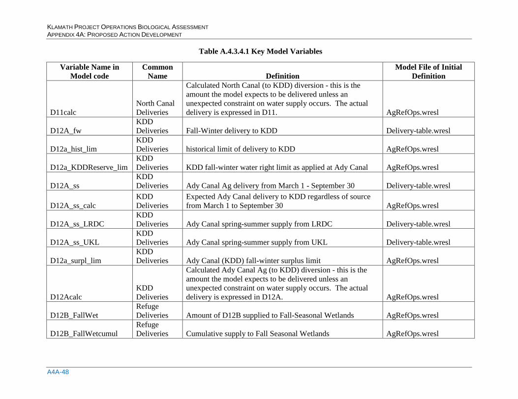
KLAMATH PROJECT OPERATIONS BIOLOGICAL ASSESSMENT APPENDIX 4A: PROPOSED ACTION DEVELOPMENT
A4A-48
Table A.4.3.4.1 Key Model Variables
Variable Name in Model code
Common Name Definition
Model File of Initial Definition
D11calc North Canal Deliveries
Calculated North Canal (to KDD) diversion - this is the amount the model expects to be delivered unless an unexpected constraint on water supply occurs. The actual delivery is expressed in D11. AgRefOps.wresl
D12A_fw KDD Deliveries Fall-Winter delivery to KDD Delivery-table.wresl
D12a_hist_lim KDD Deliveries historical limit of delivery to KDD AgRefOps.wresl
D12a_KDDReserve_lim KDD Deliveries KDD fall-winter water right limit as applied at Ady Canal AgRefOps.wresl
D12A_ss KDD Deliveries Ady Canal Ag delivery from March 1 - September 30 Delivery-table.wresl
D12A_ss_calc KDD Deliveries
Expected Ady Canal delivery to KDD regardless of source from March 1 to September 30 AgRefOps.wresl
D12A_ss_LRDC KDD Deliveries Ady Canal spring-summer supply from LRDC Delivery-table.wresl
D12A_ss_UKL KDD Deliveries Ady Canal spring-summer supply from UKL Delivery-table.wresl
D12a_surpl_lim KDD Deliveries Ady Canal (KDD) fall-winter surplus limit AgRefOps.wresl
D12Acalc KDD Deliveries
Calculated Ady Canal Ag (to KDD) diversion - this is the amount the model expects to be delivered unless an unexpected constraint on water supply occurs. The actual delivery is expressed in D12A. AgRefOps.wresl
D12B_FallWet Refuge Deliveries Amount of D12B supplied to Fall-Seasonal Wetlands AgRefOps.wresl
D12B_FallWetcumul Refuge Deliveries Cumulative supply to Fall Seasonal Wetlands AgRefOps.wresl
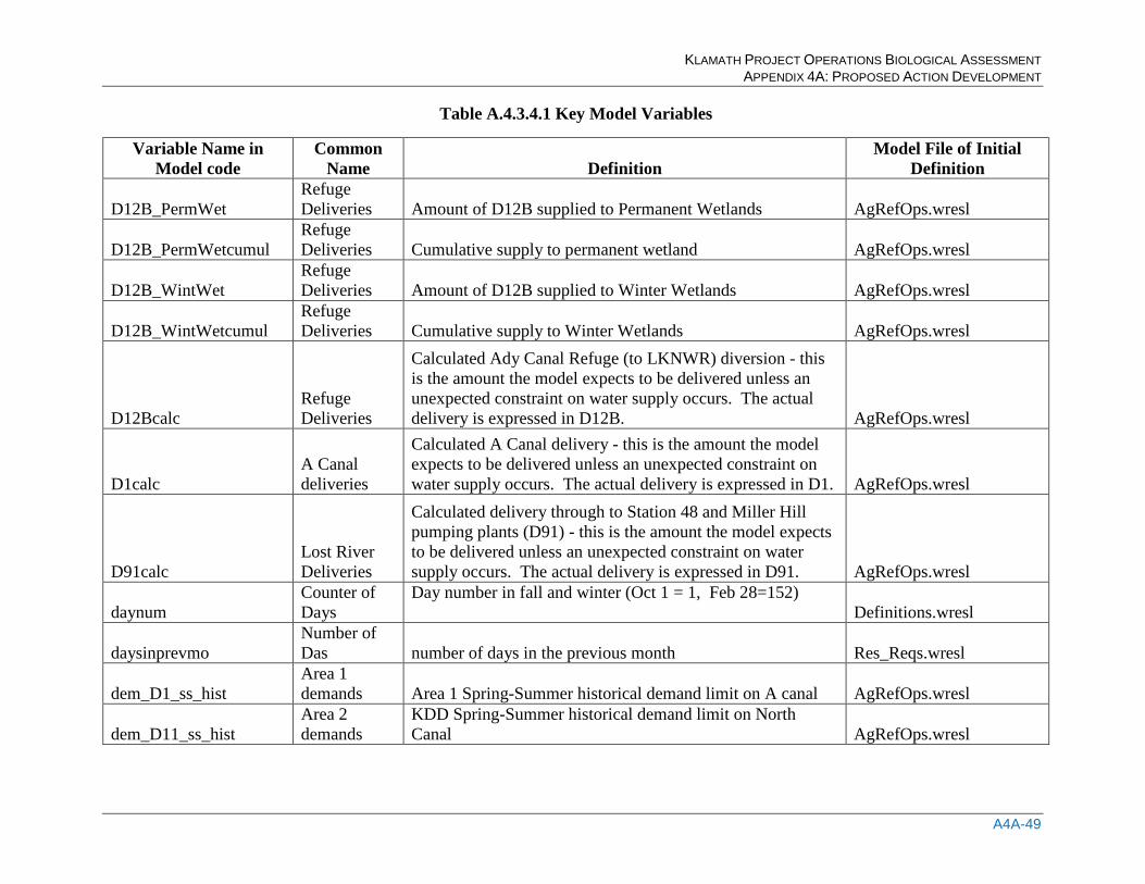
KLAMATH PROJECT OPERATIONS BIOLOGICAL ASSESSMENT APPENDIX 4A: PROPOSED ACTION DEVELOPMENT
A4A-49
Table A.4.3.4.1 Key Model Variables
Variable Name in Model code
Common Name Definition
Model File of Initial Definition
D12B_PermWet Refuge Deliveries Amount of D12B supplied to Permanent Wetlands AgRefOps.wresl
D12B_PermWetcumul Refuge Deliveries Cumulative supply to permanent wetland AgRefOps.wresl
D12B_WintWet Refuge Deliveries Amount of D12B supplied to Winter Wetlands AgRefOps.wresl
D12B_WintWetcumul Refuge Deliveries Cumulative supply to Winter Wetlands AgRefOps.wresl
D12Bcalc Refuge Deliveries
Calculated Ady Canal Refuge (to LKNWR) diversion - this is the amount the model expects to be delivered unless an unexpected constraint on water supply occurs. The actual delivery is expressed in D12B. AgRefOps.wresl
D1calc A Canal deliveries
Calculated A Canal delivery - this is the amount the model expects to be delivered unless an unexpected constraint on water supply occurs. The actual delivery is expressed in D1. AgRefOps.wresl
D91calc Lost River Deliveries
Calculated delivery through to Station 48 and Miller Hill pumping plants (D91) - this is the amount the model expects to be delivered unless an unexpected constraint on water supply occurs. The actual delivery is expressed in D91. AgRefOps.wresl
daynum Counter of Days
Day number in fall and winter (Oct 1 = 1, Feb 28=152) Definitions.wresl
daysinprevmo Number of Das number of days in the previous month Res_Reqs.wresl
dem_D1_ss_hist Area 1 demands Area 1 Spring-Summer historical demand limit on A canal AgRefOps.wresl
dem_D11_ss_hist Area 2 demands
KDD Spring-Summer historical demand limit on North Canal AgRefOps.wresl
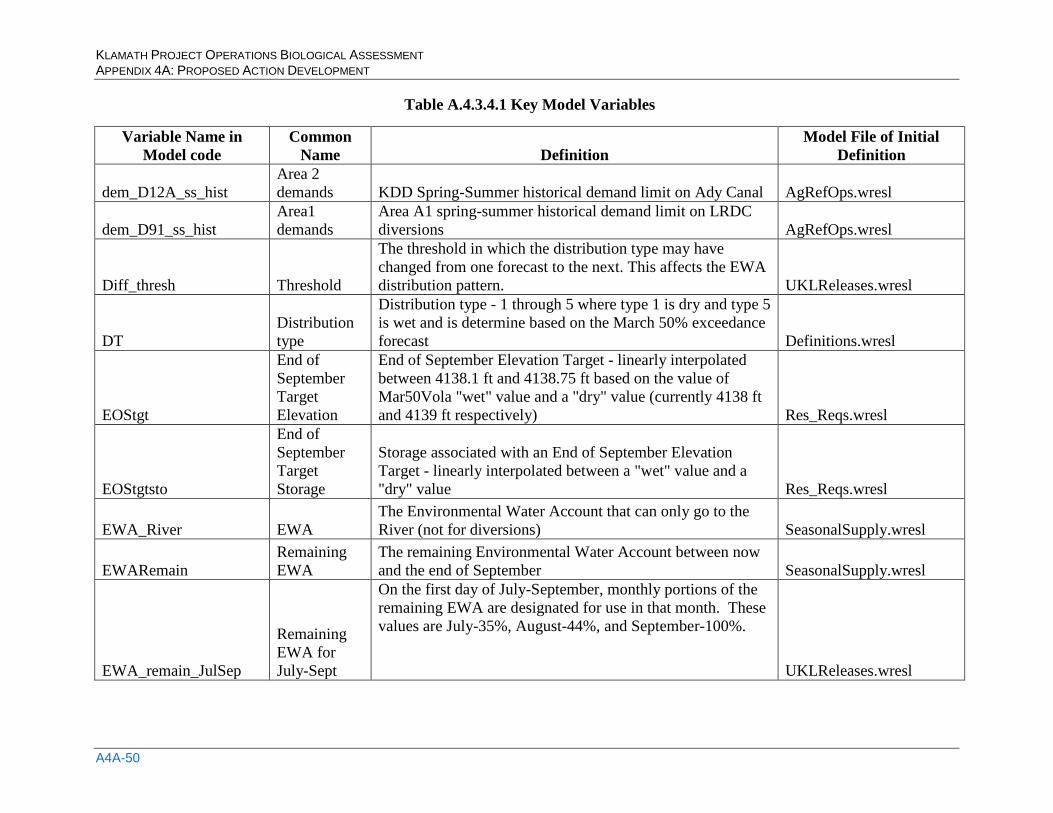
KLAMATH PROJECT OPERATIONS BIOLOGICAL ASSESSMENT APPENDIX 4A: PROPOSED ACTION DEVELOPMENT
A4A-50
Table A.4.3.4.1 Key Model Variables
Variable Name in Model code
Common Name Definition
Model File of Initial Definition
dem_D12A_ss_hist Area 2 demands KDD Spring-Summer historical demand limit on Ady Canal AgRefOps.wresl
dem_D91_ss_hist Area1 demands
Area A1 spring-summer historical demand limit on LRDC diversions AgRefOps.wresl
Diff_thresh Threshold
The threshold in which the distribution type may have changed from one forecast to the next. This affects the EWA distribution pattern. UKLReleases.wresl
DT Distribution type
Distribution type - 1 through 5 where type 1 is dry and type 5 is wet and is determine based on the March 50% exceedance forecast Definitions.wresl
EOStgt
End of September Target Elevation
End of September Elevation Target - linearly interpolated between 4138.1 ft and 4138.75 ft based on the value of Mar50Vola "wet" value and a "dry" value (currently 4138 ft and 4139 ft respectively) Res_Reqs.wresl
EOStgtsto
End of September Target Storage
Storage associated with an End of September Elevation Target - linearly interpolated between a "wet" value and a "dry" value Res_Reqs.wresl
EWA_River EWA The Environmental Water Account that can only go to the River (not for diversions) SeasonalSupply.wresl
EWARemain Remaining EWA
The remaining Environmental Water Account between now and the end of September SeasonalSupply.wresl
EWA_remain_JulSep
Remaining EWA for July-Sept
On the first day of July-September, monthly portions of the remaining EWA are designated for use in that month. These values are July-35%, August-44%, and September-100%.
UKLReleases.wresl
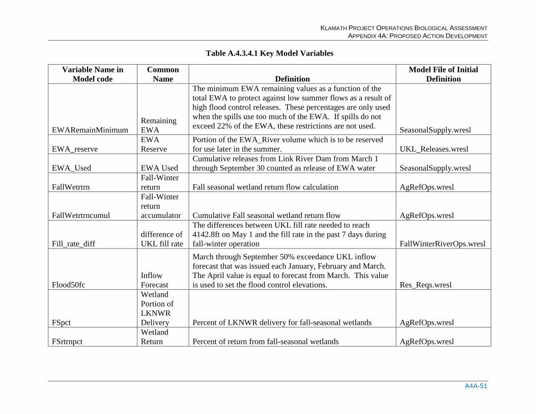
KLAMATH PROJECT OPERATIONS BIOLOGICAL ASSESSMENT APPENDIX 4A: PROPOSED ACTION DEVELOPMENT
A4A-51
Table A.4.3.4.1 Key Model Variables
Variable Name in Model code
Common Name Definition
Model File of Initial Definition
EWARemainMinimum Remaining EWA
The minimum EWA remaining values as a function of the total EWA to protect against low summer flows as a result of high flood control releases. These percentages are only used when the spills use too much of the EWA. If spills do not exceed 22% of the EWA, these restrictions are not used. SeasonalSupply.wresl
EWA_reserve EWA Reserve
Portion of the EWA_River volume which is to be reserved for use later in the summer. UKL_Releases.wresl
EWA_Used EWA Used Cumulative releases from Link River Dam from March 1 through September 30 counted as release of EWA water SeasonalSupply.wresl
FallWetrtrn Fall-Winter return Fall seasonal wetland return flow calculation AgRefOps.wresl
FallWetrtrncumul
Fall-Winter return accumulator Cumulative Fall seasonal wetland return flow AgRefOps.wresl
Fill_rate_diff difference of UKL fill rate
The differences between UKL fill rate needed to reach 4142.8ft on May 1 and the fill rate in the past 7 days during fall-winter operation FallWinterRiverOps.wresl
Flood50fc Inflow Forecast
March through September 50% exceedance UKL inflow forecast that was issued each January, February and March. The April value is equal to forecast from March. This value is used to set the flood control elevations. Res_Reqs.wresl
FSpct
Wetland Portion of LKNWR Delivery Percent of LKNWR delivery for fall-seasonal wetlands AgRefOps.wresl
FSrtrnpct Wetland Return Percent of return from fall-seasonal wetlands AgRefOps.wresl
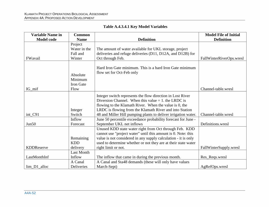
KLAMATH PROJECT OPERATIONS BIOLOGICAL ASSESSMENT APPENDIX 4A: PROPOSED ACTION DEVELOPMENT
A4A-52
Table A.4.3.4.1 Key Model Variables
Variable Name in Model code
Common Name Definition
Model File of Initial Definition
FWavail
Project Water in the Fall and Winter
The amount of water available for UKL storage, project deliveries and refuge deliveries (D11, D12A, and D12B) for Oct through Feb. FallWinterRiverOps.wresl
IG_mif
Absolute Minimum Iron Gate Flow
Hard Iron Gate minimum. This is a hard Iron Gate minimum flow set for Oct-Feb only
Channel-table.wresl
int_C91 Integer Switch
Integer switch represents the flow direction in Lost River Diversion Channel. When this value = 1. the LRDC is flowing to the Klamath River. When the value is 0, the LRDC is flowing from the Klamath River and into Station 48 and Miller Hill pumping plants to deliver irrigation water. Channel-table.wresl
Jun50 Inflow Forecast
June 50 percentile exceedance probability forecast for June -September UKL net inflows Definitions.wresl
KDDReserve
Remaining KDD delivery
Unused KDD state water right from Oct through Feb. KDD cannot use "project water" until this amount is 0. Note: this value is not considered in any supply calculation - it is only used to determine whether or not they are at their state water right limit or not. FallWinterSupply.wresl
LastMonthInf Last Month Inflow The inflow that came in during the previous month. Res_Reqs.wresl
lim_D1_alloc A Canal Deliveries
A Canal and Sta48 demands (these will only have values March-Sept) AgRefOps.wresl
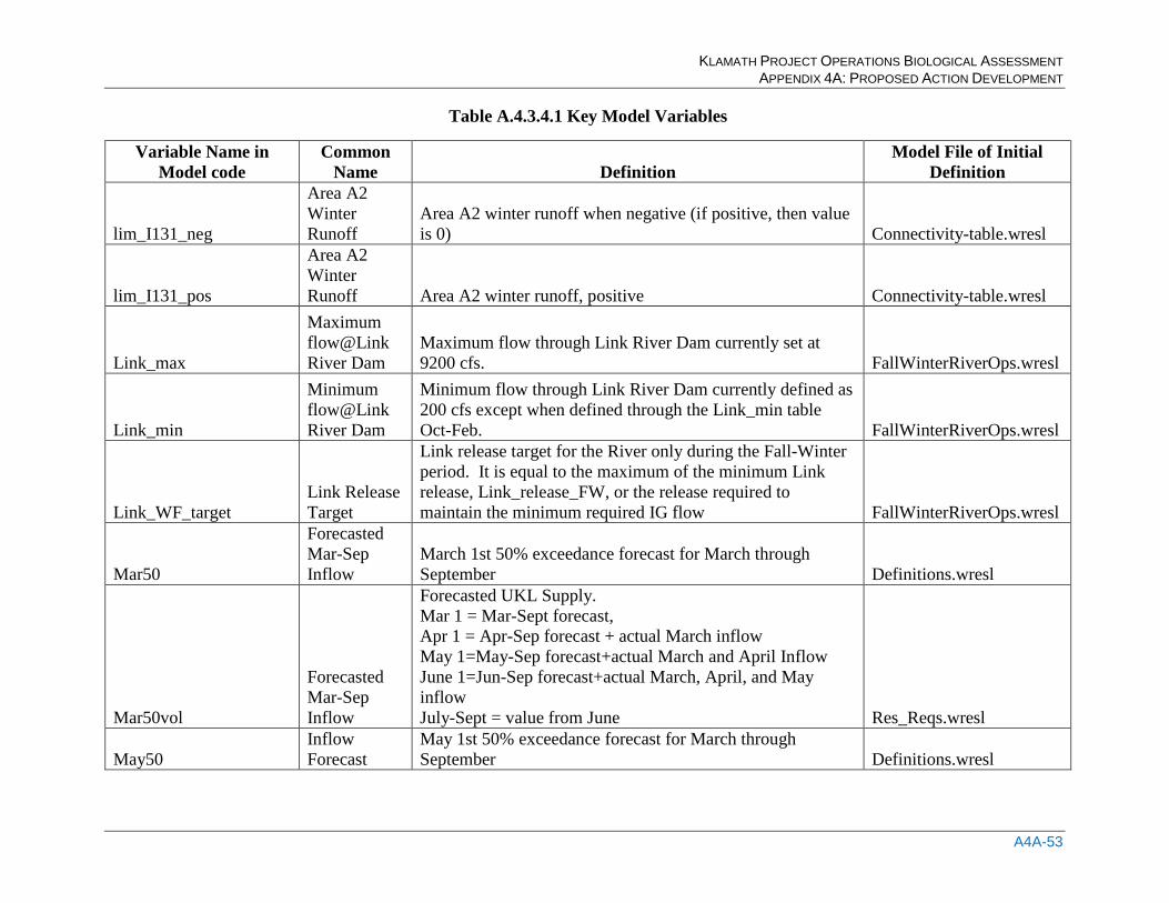
KLAMATH PROJECT OPERATIONS BIOLOGICAL ASSESSMENT APPENDIX 4A: PROPOSED ACTION DEVELOPMENT
A4A-53
Table A.4.3.4.1 Key Model Variables
Variable Name in Model code
Common Name Definition
Model File of Initial Definition
lim_I131_neg
Area A2 Winter Runoff
Area A2 winter runoff when negative (if positive, then value is 0) Connectivity-table.wresl
lim_I131_pos
Area A2 Winter Runoff Area A2 winter runoff, positive Connectivity-table.wresl
Link_max
Maximum flow@Link River Dam
Maximum flow through Link River Dam currently set at 9200 cfs. FallWinterRiverOps.wresl
Link_min
Minimum flow@Link River Dam
Minimum flow through Link River Dam currently defined as 200 cfs except when defined through the Link_min table Oct-Feb. FallWinterRiverOps.wresl
Link_WF_target Link Release Target
Link release target for the River only during the Fall-Winter period. It is equal to the maximum of the minimum Link release, Link_release_FW, or the release required to maintain the minimum required IG flow FallWinterRiverOps.wresl
Mar50
Forecasted Mar-Sep Inflow
March 1st 50% exceedance forecast for March through September Definitions.wresl
Mar50vol
Forecasted Mar-Sep Inflow
Forecasted UKL Supply. Mar 1 = Mar-Sept forecast, Apr 1 = Apr-Sep forecast + actual March inflow May 1=May-Sep forecast+actual March and April Inflow June 1=Jun-Sep forecast+actual March, April, and May inflow July-Sept = value from June Res_Reqs.wresl
May50 Inflow Forecast
May 1st 50% exceedance forecast for March through September Definitions.wresl
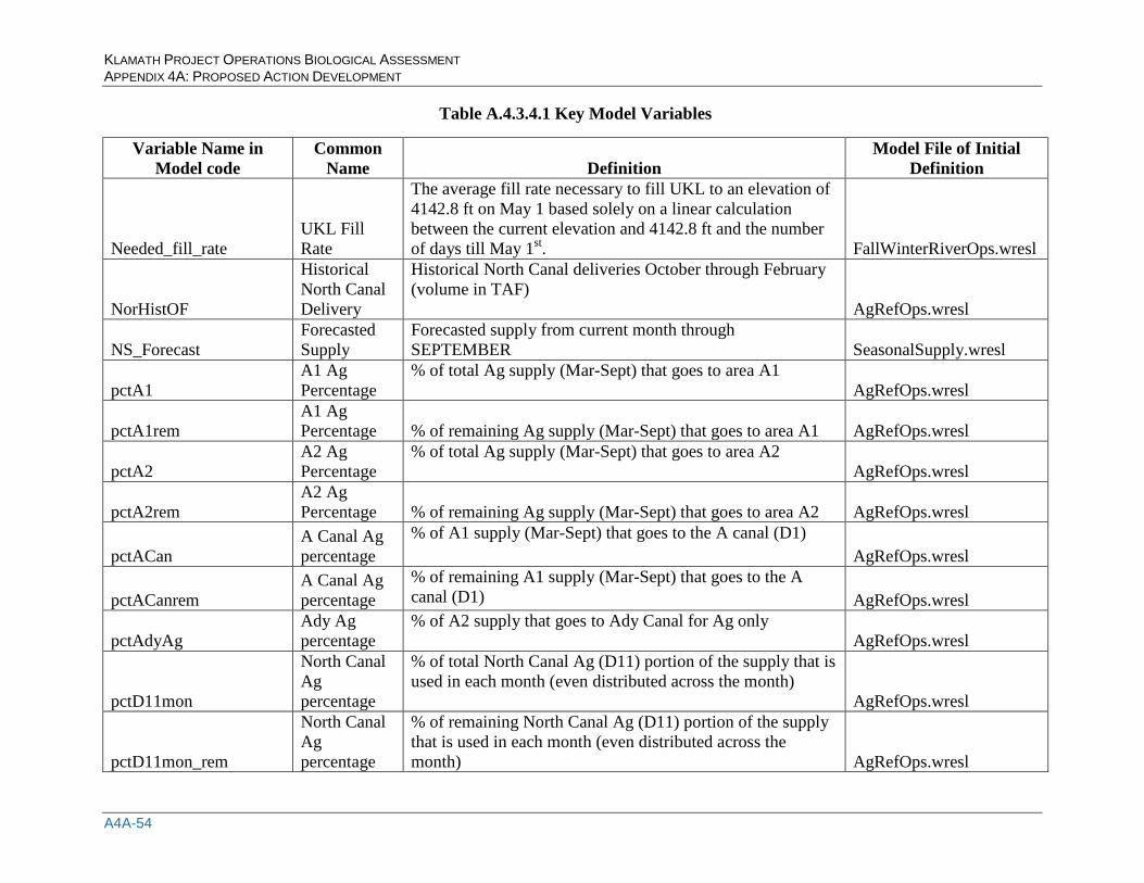
KLAMATH PROJECT OPERATIONS BIOLOGICAL ASSESSMENT APPENDIX 4A: PROPOSED ACTION DEVELOPMENT
A4A-54
Table A.4.3.4.1 Key Model Variables
Variable Name in Model code
Common Name Definition
Model File of Initial Definition
Needed_fill_rate UKL Fill Rate
The average fill rate necessary to fill UKL to an elevation of 4142.8 ft on May 1 based solely on a linear calculation between the current elevation and 4142.8 ft and the number of days till May 1st. FallWinterRiverOps.wresl
NorHistOF
Historical North Canal Delivery
Historical North Canal deliveries October through February (volume in TAF)
AgRefOps.wresl
NS_Forecast Forecasted Supply
Forecasted supply from current month through SEPTEMBER SeasonalSupply.wresl
pctA1 A1 Ag Percentage
% of total Ag supply (Mar-Sept) that goes to area A1 AgRefOps.wresl
pctA1rem A1 Ag Percentage % of remaining Ag supply (Mar-Sept) that goes to area A1 AgRefOps.wresl
pctA2 A2 Ag Percentage
% of total Ag supply (Mar-Sept) that goes to area A2 AgRefOps.wresl
pctA2rem A2 Ag Percentage % of remaining Ag supply (Mar-Sept) that goes to area A2 AgRefOps.wresl
pctACan A Canal Ag percentage
% of A1 supply (Mar-Sept) that goes to the A canal (D1) AgRefOps.wresl
pctACanrem A Canal Ag percentage
% of remaining A1 supply (Mar-Sept) that goes to the A canal (D1) AgRefOps.wresl
pctAdyAg Ady Ag percentage
% of A2 supply that goes to Ady Canal for Ag only AgRefOps.wresl
pctD11mon
North Canal Ag percentage
% of total North Canal Ag (D11) portion of the supply that is used in each month (even distributed across the month)
AgRefOps.wresl
pctD11mon_rem
North Canal Ag percentage
% of remaining North Canal Ag (D11) portion of the supply that is used in each month (even distributed across the month) AgRefOps.wresl
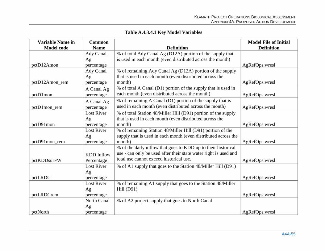
KLAMATH PROJECT OPERATIONS BIOLOGICAL ASSESSMENT APPENDIX 4A: PROPOSED ACTION DEVELOPMENT
A4A-55
Table A.4.3.4.1 Key Model Variables
Variable Name in Model code
Common Name Definition
Model File of Initial Definition
pctD12Amon
Ady Canal Ag percentage
% of total Ady Canal Ag (D12A) portion of the supply that is used in each month (even distributed across the month)
AgRefOps.wresl
pctD12Amon_rem
Ady Canal Ag percentage
% of remaining Ady Canal Ag (D12A) portion of the supply that is used in each month (even distributed across the month) AgRefOps.wresl
pctD1mon A Canal Ag percentage
% of total A Canal (D1) portion of the supply that is used in each month (even distributed across the month) AgRefOps.wresl
pctD1mon_rem A Canal Ag percentage
% of remaining A Canal (D1) portion of the supply that is used in each month (even distributed across the month) AgRefOps.wresl
pctD91mon
Lost River Ag percentage
% of total Station 48/Miller Hill (D91) portion of the supply that is used in each month (even distributed across the month) AgRefOps.wresl
pctD91mon_rem
Lost River Ag percentage
% of remaining Station 48/Miller Hill (D91) portion of the supply that is used in each month (even distributed across the month) AgRefOps.wresl
pctKDDsurFW KDD Inflow Percentage
% of the daily inflow that goes to KDD up to their historical use - can only be used after their state water right is used and total use cannot exceed historical use. AgRefOps.wresl
pctLRDC
Lost River Ag percentage
% of A1 supply that goes to the Station 48/Miller Hill (D91)
AgRefOps.wresl
pctLRDCrem
Lost River Ag percentage
% of remaining A1 supply that goes to the Station 48/Miller Hill (D91)
AgRefOps.wresl
pctNorth
North Canal Ag percentage
% of A2 project supply that goes to North Canal
AgRefOps.wresl
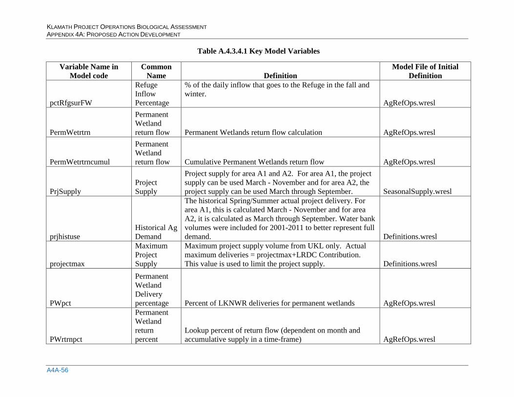
KLAMATH PROJECT OPERATIONS BIOLOGICAL ASSESSMENT APPENDIX 4A: PROPOSED ACTION DEVELOPMENT
A4A-56
Table A.4.3.4.1 Key Model Variables
Variable Name in Model code
Common Name Definition
Model File of Initial Definition
pctRfgsurFW
Refuge Inflow Percentage
% of the daily inflow that goes to the Refuge in the fall and winter.
AgRefOps.wresl
PermWetrtrn
Permanent Wetland return flow Permanent Wetlands return flow calculation AgRefOps.wresl
PermWetrtrncumul
Permanent Wetland return flow Cumulative Permanent Wetlands return flow AgRefOps.wresl
PrjSupply Project Supply
Project supply for area A1 and A2. For area A1, the project supply can be used March - November and for area A2, the project supply can be used March through September. SeasonalSupply.wresl
prjhistuse Historical Ag Demand
The historical Spring/Summer actual project delivery. For area A1, this is calculated March - November and for area A2, it is calculated as March through September. Water bank volumes were included for 2001-2011 to better represent full demand. Definitions.wresl
projectmax
Maximum Project Supply
Maximum project supply volume from UKL only. Actual maximum deliveries = projectmax+LRDC Contribution. This value is used to limit the project supply. Definitions.wresl
PWpct
Permanent Wetland Delivery percentage Percent of LKNWR deliveries for permanent wetlands AgRefOps.wresl
PWrtrnpct
Permanent Wetland return percent
Lookup percent of return flow (dependent on month and accumulative supply in a time-frame) AgRefOps.wresl
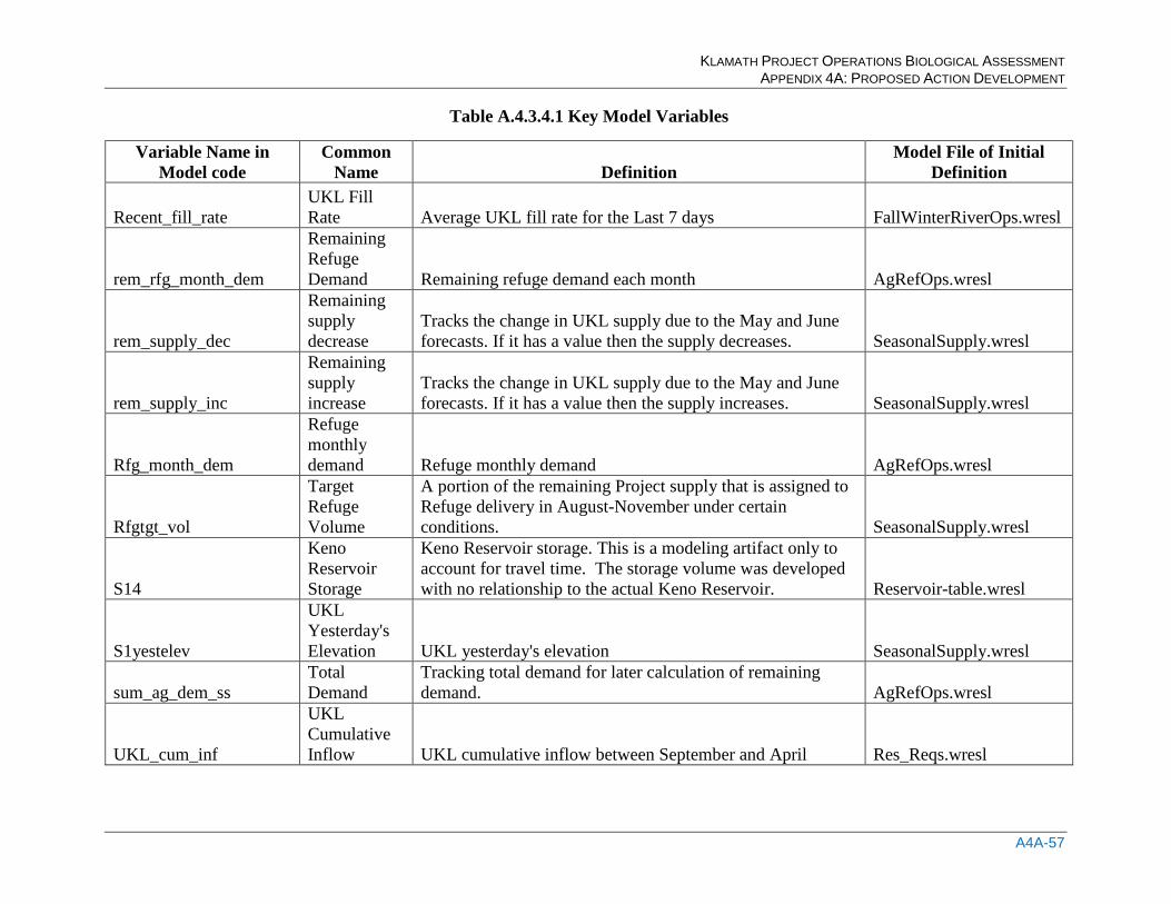
KLAMATH PROJECT OPERATIONS BIOLOGICAL ASSESSMENT APPENDIX 4A: PROPOSED ACTION DEVELOPMENT
A4A-57
Table A.4.3.4.1 Key Model Variables
Variable Name in Model code
Common Name Definition
Model File of Initial Definition
Recent_fill_rate UKL Fill Rate Average UKL fill rate for the Last 7 days FallWinterRiverOps.wresl
rem_rfg_month_dem
Remaining Refuge Demand Remaining refuge demand each month AgRefOps.wresl
rem_supply_dec
Remaining supply decrease
Tracks the change in UKL supply due to the May and June forecasts. If it has a value then the supply decreases. SeasonalSupply.wresl
rem_supply_inc
Remaining supply increase
Tracks the change in UKL supply due to the May and June forecasts. If it has a value then the supply increases. SeasonalSupply.wresl
Rfg_month_dem
Refuge monthly demand Refuge monthly demand AgRefOps.wresl
Rfgtgt_vol
Target Refuge Volume
A portion of the remaining Project supply that is assigned to Refuge delivery in August-November under certain conditions. SeasonalSupply.wresl
S14
Keno Reservoir Storage
Keno Reservoir storage. This is a modeling artifact only to account for travel time. The storage volume was developed with no relationship to the actual Keno Reservoir. Reservoir-table.wresl
S1yestelev
UKL Yesterday's Elevation UKL yesterday's elevation SeasonalSupply.wresl
sum_ag_dem_ss Total Demand
Tracking total demand for later calculation of remaining demand. AgRefOps.wresl
UKL_cum_inf
UKL Cumulative Inflow UKL cumulative inflow between September and April Res_Reqs.wresl
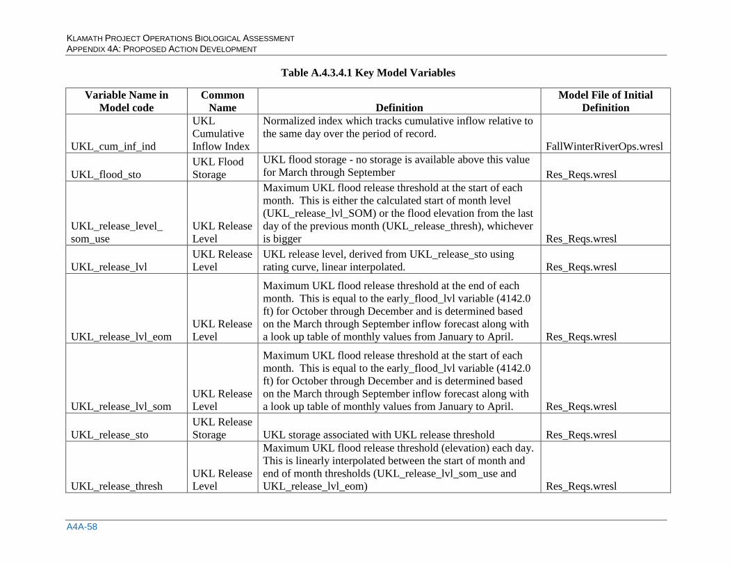
KLAMATH PROJECT OPERATIONS BIOLOGICAL ASSESSMENT APPENDIX 4A: PROPOSED ACTION DEVELOPMENT
A4A-58
Table A.4.3.4.1 Key Model Variables
Variable Name in Model code
Common Name Definition
Model File of Initial Definition
UKL_cum_inf_ind
UKL Cumulative Inflow Index
Normalized index which tracks cumulative inflow relative to the same day over the period of record.
FallWinterRiverOps.wresl
UKL_flood_sto UKL Flood Storage
UKL flood storage - no storage is available above this value for March through September Res_Reqs.wresl
UKL_release_level_ som_use
UKL Release Level
Maximum UKL flood release threshold at the start of each month. This is either the calculated start of month level (UKL_release_lvl_SOM) or the flood elevation from the last day of the previous month (UKL_release_thresh), whichever is bigger Res_Reqs.wresl
UKL_release_lvl UKL Release Level
UKL release level, derived from UKL_release_sto using rating curve, linear interpolated. Res_Reqs.wresl
UKL_release_lvl_eom UKL Release Level
Maximum UKL flood release threshold at the end of each month. This is equal to the early_flood_lvl variable (4142.0 ft) for October through December and is determined based on the March through September inflow forecast along with a look up table of monthly values from January to April. Res_Reqs.wresl
UKL_release_lvl_som UKL Release Level
Maximum UKL flood release threshold at the start of each month. This is equal to the early_flood_lvl variable (4142.0 ft) for October through December and is determined based on the March through September inflow forecast along with a look up table of monthly values from January to April. Res_Reqs.wresl
UKL_release_sto UKL Release Storage UKL storage associated with UKL release threshold Res_Reqs.wresl
UKL_release_thresh UKL Release Level
Maximum UKL flood release threshold (elevation) each day. This is linearly interpolated between the start of month and end of month thresholds (UKL_release_lvl_som_use and UKL_release_lvl_eom) Res_Reqs.wresl
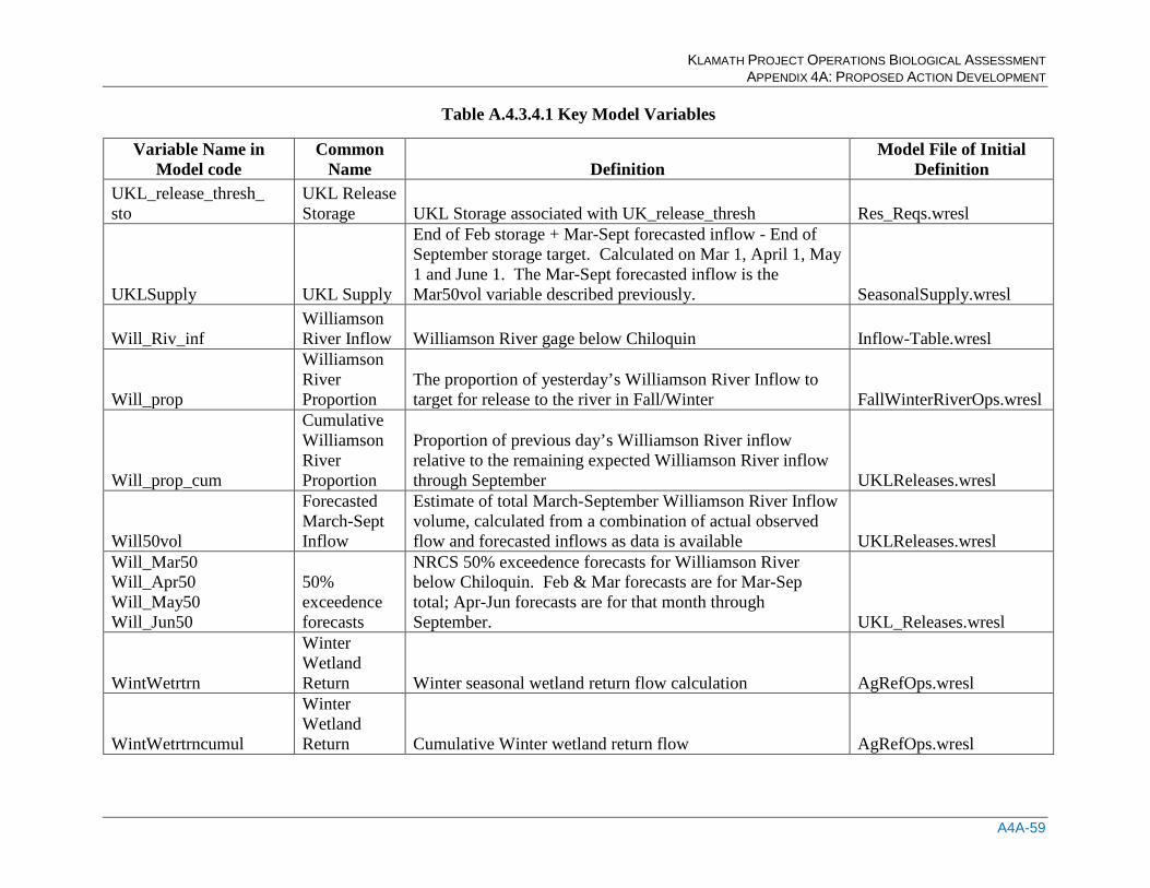
KLAMATH PROJECT OPERATIONS BIOLOGICAL ASSESSMENT APPENDIX 4A: PROPOSED ACTION DEVELOPMENT
A4A-59
Table A.4.3.4.1 Key Model Variables
Variable Name in Model code
Common Name Definition
Model File of Initial Definition
UKL_release_thresh_ sto
UKL Release Storage UKL Storage associated with UK_release_thresh Res_Reqs.wresl
UKLSupply UKL Supply
End of Feb storage + Mar-Sept forecasted inflow - End of September storage target. Calculated on Mar 1, April 1, May 1 and June 1. The Mar-Sept forecasted inflow is the Mar50vol variable described previously. SeasonalSupply.wresl
Will_Riv_inf Williamson River Inflow Williamson River gage below Chiloquin Inflow-Table.wresl
Will_prop
Williamson River Proportion
The proportion of yesterday’s Williamson River Inflow to target for release to the river in Fall/Winter FallWinterRiverOps.wresl
Will_prop_cum
Cumulative Williamson River Proportion
Proportion of previous day’s Williamson River inflow relative to the remaining expected Williamson River inflow through September UKLReleases.wresl
Will50vol
Forecasted March-Sept Inflow
Estimate of total March-September Williamson River Inflow volume, calculated from a combination of actual observed flow and forecasted inflows as data is available UKLReleases.wresl
Will_Mar50 Will_Apr50 Will_May50 Will_Jun50
50% exceedence forecasts
NRCS 50% exceedence forecasts for Williamson River below Chiloquin. Feb & Mar forecasts are for Mar-Sep total; Apr-Jun forecasts are for that month through September. UKL_Releases.wresl
WintWetrtrn
Winter Wetland Return Winter seasonal wetland return flow calculation AgRefOps.wresl
WintWetrtrncumul
Winter Wetland Return Cumulative Winter wetland return flow AgRefOps.wresl
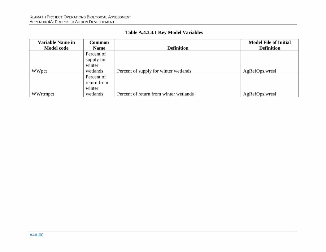
KLAMATH PROJECT OPERATIONS BIOLOGICAL ASSESSMENT APPENDIX 4A: PROPOSED ACTION DEVELOPMENT
A4A-60
Table A.4.3.4.1 Key Model Variables
Variable Name in Model code
Common Name Definition
Model File of Initial Definition
WWpct
Percent of supply for winter wetlands Percent of supply for winter wetlands AgRefOps.wresl
WWrtrnpct
Percent of return from winter wetlands Percent of return from winter wetlands AgRefOps.wresl
KLAMATH PROJECT OPERATIONS BIOLOGICAL ASSESSMENT APPENDIX 4A: PROPOSED ACTION DEVELOPMENT
A4A-61
Section B: Proposed Action Model Output Graphs

KLAMATH PROJECT OPERATIONS BIOLOGICAL ASSESSMENT APPENDIX 4A: PROPOSED ACTION DEVELOPMENT
A4A-62
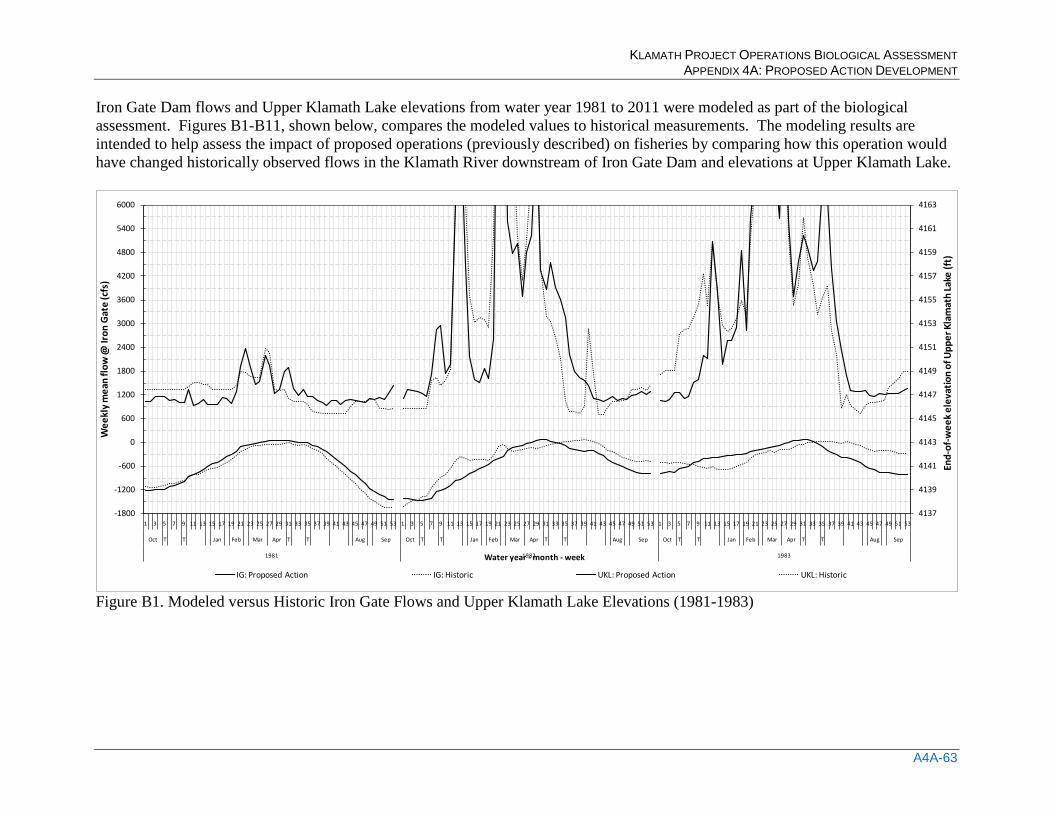
KLAMATH PROJECT OPERATIONS BIOLOGICAL ASSESSMENT APPENDIX 4A: PROPOSED ACTION DEVELOPMENT
A4A-63
Iron Gate Dam flows and Upper Klamath Lake elevations from water year 1981 to 2011 were modeled as part of the biological assessment. Figures B1-B11, shown below, compares the modeled values to historical measurements. The modeling results are intended to help assess the impact of proposed operations (previously described) on fisheries by comparing how this operation would have changed historically observed flows in the Klamath River downstream of Iron Gate Dam and elevations at Upper Klamath Lake.
4137
4139
4141
4143
4145
4147
4149
4151
4153
4155
4157
4159
4161
4163
-1800
-1200
-600
0
600
1200
1800
2400
3000
3600
4200
4800
5400
6000
1 3 5 7 9 11 13 15 17 19 21 23 25 27 29 31 33 35 37 39 41 43 45 47 49 51 53 1 3 5 7 9 11 13 15 17 19 21 23 25 27 29 31 33 35 37 39 41 43 45 47 49 51 53 1 3 5 7 9 11 13 15 17 19 21 23 25 27 29 31 33 35 37 39 41 43 45 47 49 51 53
Oct T T Jan Feb Mar Apr T T Aug Sep Oct T T Jan Feb Mar Apr T T Aug Sep Oct T T Jan Feb Mar Apr T T Aug Sep
1981 1982 1983
End-
of-w
eek e
leva
tion
of U
pper
Kla
mat
h La
ke (f
t)
Wee
kly m
ean
flow
@ Ir
on G
ate
(cfs
)
Water year - month - week
IG: Proposed Action IG: Historic UKL: Proposed Action UKL: Historic
Figure B1. Modeled versus Historic Iron Gate Flows and Upper Klamath Lake Elevations (1981-1983)
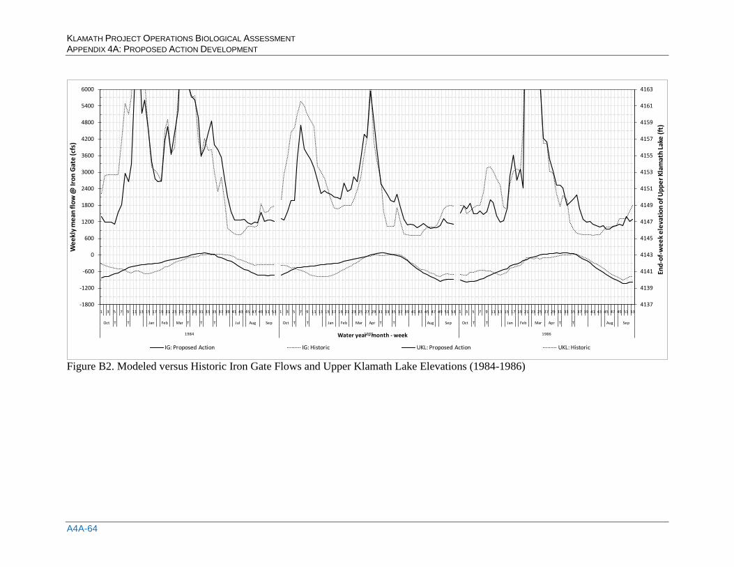
KLAMATH PROJECT OPERATIONS BIOLOGICAL ASSESSMENT APPENDIX 4A: PROPOSED ACTION DEVELOPMENT
A4A-64
4137
4139
4141
4143
4145
4147
4149
4151
4153
4155
4157
4159
4161
4163
-1800
-1200
-600
0
600
1200
1800
2400
3000
3600
4200
4800
5400
6000
1 3 5 7 9 11 13 15 17 19 21 23 25 27 29 31 33 35 37 39 41 43 45 47 49 51 53 1 3 5 7 9 11 13 15 17 19 21 23 25 27 29 31 33 35 37 39 41 43 45 47 49 51 53 1 3 5 7 9 11 13 15 17 19 21 23 25 27 29 31 33 35 37 39 41 43 45 47 49 51 53
Oct T T Jan Feb Mar T T T Jul Aug Sep Oct T T Jan Feb Mar Apr T T Aug Sep Oct T T Jan Feb Mar Apr T T Aug Sep
1984 1985 1986
End -
of-w
eek e
leva
tion
of U
pper
Kla
mat
h La
ke (f
t)
Wee
kly m
ean
flow
@ Ir
on G
ate
(cfs
)
Water year - month - week
IG: Proposed Action IG: Historic UKL: Proposed Action UKL: Historic
Figure B2. Modeled versus Historic Iron Gate Flows and Upper Klamath Lake Elevations (1984-1986)
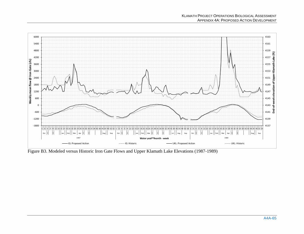
KLAMATH PROJECT OPERATIONS BIOLOGICAL ASSESSMENT APPENDIX 4A: PROPOSED ACTION DEVELOPMENT
A4A-65
4137
4139
4141
4143
4145
4147
4149
4151
4153
4155
4157
4159
4161
4163
-1800
-1200
-600
0
600
1200
1800
2400
3000
3600
4200
4800
5400
6000
1 3 5 7 9 11 13 15 17 19 21 23 25 27 29 31 33 35 37 39 41 43 45 47 49 51 53 1 3 5 7 9 11 13 15 17 19 21 23 25 27 29 31 33 35 37 39 41 43 45 47 49 51 53 1 3 5 7 9 11 13 15 17 19 21 23 25 27 29 31 33 35 37 39 41 43 45 47 49 51 53
Oct T T Jan Feb Mar Apr T T Aug Sep Oct T T Jan Feb Mar T T T Jul Aug Sep Oct T T Jan Feb Mar Apr T T Aug Sep
1987 1988 1989
End -
of-w
eek e
leva
tion
of U
pper
Kla
mat
h La
ke (f
t)
Wee
kly m
ean
flow
@ Ir
on G
ate
(cfs
)
Water year - month - week
IG: Proposed Action IG: Historic UKL: Proposed Action UKL: Historic
Figure B3. Modeled versus Historic Iron Gate Flows and Upper Klamath Lake Elevations (1987-1989)
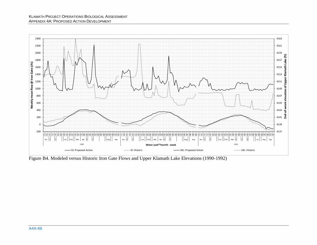
KLAMATH PROJECT OPERATIONS BIOLOGICAL ASSESSMENT APPENDIX 4A: PROPOSED ACTION DEVELOPMENT
A4A-66
4137
4139
4141
4143
4145
4147
4149
4151
4153
4155
4157
4159
4161
4163
-200
0
200
400
600
800
1000
1200
1400
1600
1800
2000
2200
2400
1 3 5 7 9 11 13 15 17 19 21 23 25 27 29 31 33 35 37 39 41 43 45 47 49 51 53 1 3 5 7 9 11 13 15 17 19 21 23 25 27 29 31 33 35 37 39 41 43 45 47 49 51 53 1 3 5 7 9 11 13 15 17 19 21 23 25 27 29 31 33 35 37 39 41 43 45 47 49 51 53
Oct T T Jan Feb Mar Apr T T Aug Sep Oct T T Jan Feb Mar Apr T T Aug Sep Oct T T Jan Feb Mar T T T Jul Aug Sep
1990 1991 1992
End -
of-w
eek e
leva
tion
of U
pper
Kla
mat
h La
ke (f
t)
Wee
kly m
ean
flow
@ Ir
on G
ate
(cfs
)
Water year - month - week
IG: Proposed Action IG: Historic UKL: Proposed Action UKL: Historic
Figure B4. Modeled versus Historic Iron Gate Flows and Upper Klamath Lake Elevations (1990-1992)
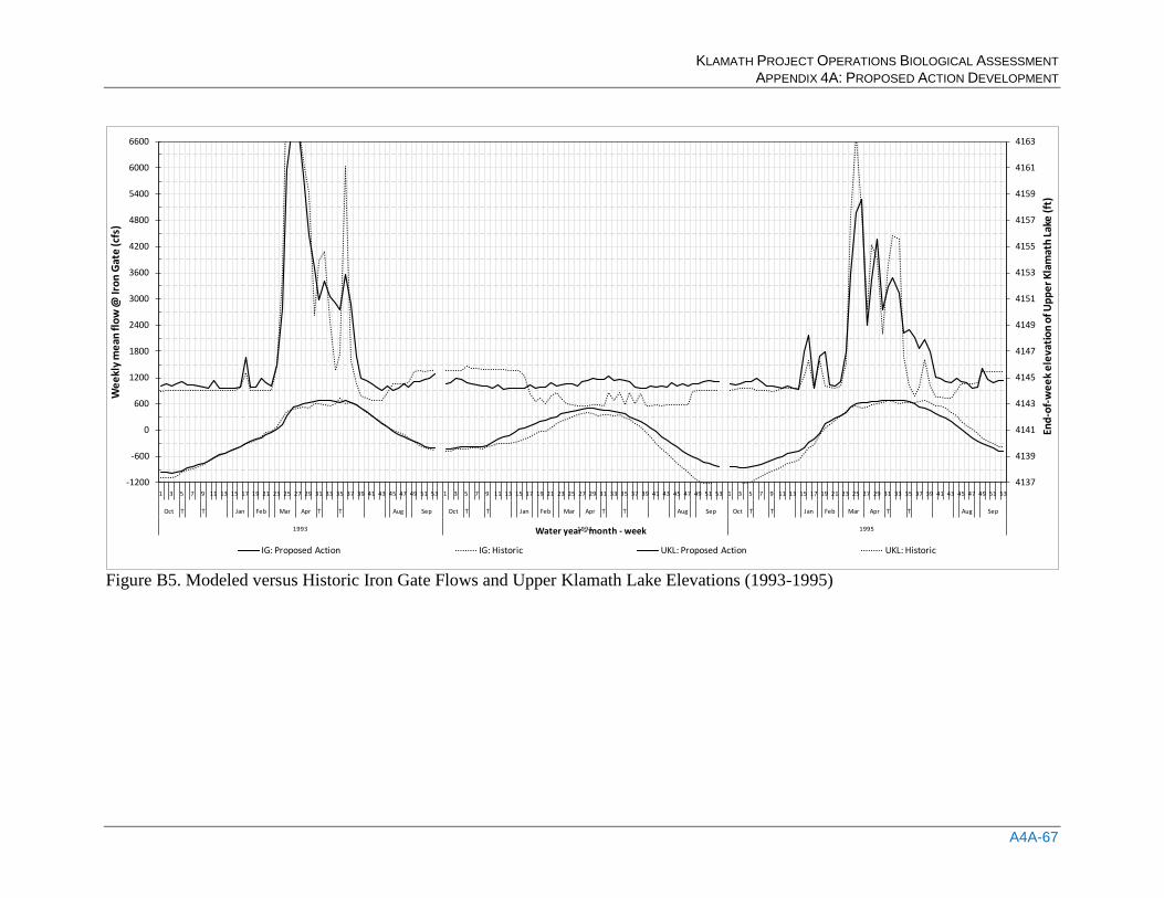
KLAMATH PROJECT OPERATIONS BIOLOGICAL ASSESSMENT APPENDIX 4A: PROPOSED ACTION DEVELOPMENT
A4A-67
4137
4139
4141
4143
4145
4147
4149
4151
4153
4155
4157
4159
4161
4163
-1200
-600
0
600
1200
1800
2400
3000
3600
4200
4800
5400
6000
6600
1 3 5 7 9 11 13 15 17 19 21 23 25 27 29 31 33 35 37 39 41 43 45 47 49 51 53 1 3 5 7 9 11 13 15 17 19 21 23 25 27 29 31 33 35 37 39 41 43 45 47 49 51 53 1 3 5 7 9 11 13 15 17 19 21 23 25 27 29 31 33 35 37 39 41 43 45 47 49 51 53
Oct T T Jan Feb Mar Apr T T Aug Sep Oct T T Jan Feb Mar Apr T T Aug Sep Oct T T Jan Feb Mar Apr T T Aug Sep
1993 1994 1995
End -
of-w
eek e
leva
tion
of U
pper
Kla
mat
h La
ke (f
t)
Wee
kly m
ean
flow
@ Ir
on G
ate
(cfs
)
Water year - month - week
IG: Proposed Action IG: Historic UKL: Proposed Action UKL: Historic
Figure B5. Modeled versus Historic Iron Gate Flows and Upper Klamath Lake Elevations (1993-1995)
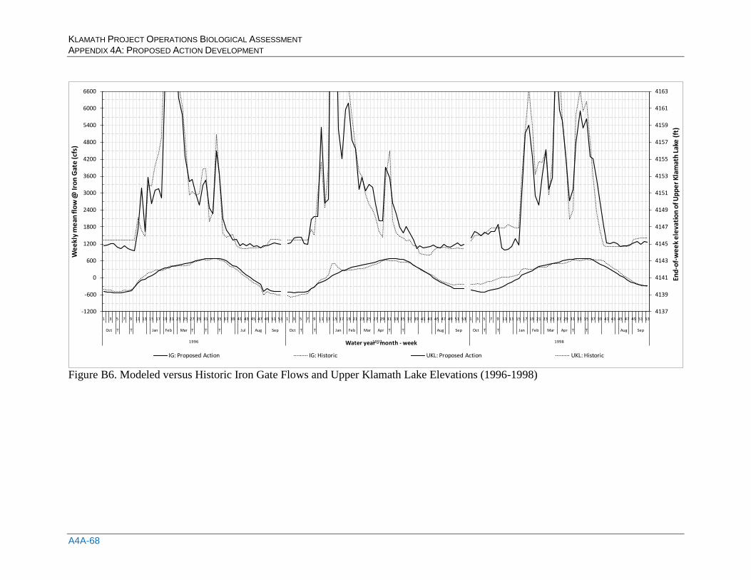
KLAMATH PROJECT OPERATIONS BIOLOGICAL ASSESSMENT APPENDIX 4A: PROPOSED ACTION DEVELOPMENT
A4A-68
4137
4139
4141
4143
4145
4147
4149
4151
4153
4155
4157
4159
4161
4163
-1200
-600
0
600
1200
1800
2400
3000
3600
4200
4800
5400
6000
6600
1 3 5 7 9 11 13 15 17 19 21 23 25 27 29 31 33 35 37 39 41 43 45 47 49 51 53 1 3 5 7 9 11 13 15 17 19 21 23 25 27 29 31 33 35 37 39 41 43 45 47 49 51 53 1 3 5 7 9 11 13 15 17 19 21 23 25 27 29 31 33 35 37 39 41 43 45 47 49 51 53
Oct T T Jan Feb Mar T T T Jul Aug Sep Oct T T Jan Feb Mar Apr T T Aug Sep Oct T T Jan Feb Mar Apr T T Aug Sep
1996 1997 1998
End -
of-w
eek e
leva
tion
of U
pper
Kla
mat
h La
ke (f
t)
Wee
kly m
ean
flow
@ Ir
on G
ate
(cfs
)
Water year - month - week
IG: Proposed Action IG: Historic UKL: Proposed Action UKL: Historic
Figure B6. Modeled versus Historic Iron Gate Flows and Upper Klamath Lake Elevations (1996-1998)
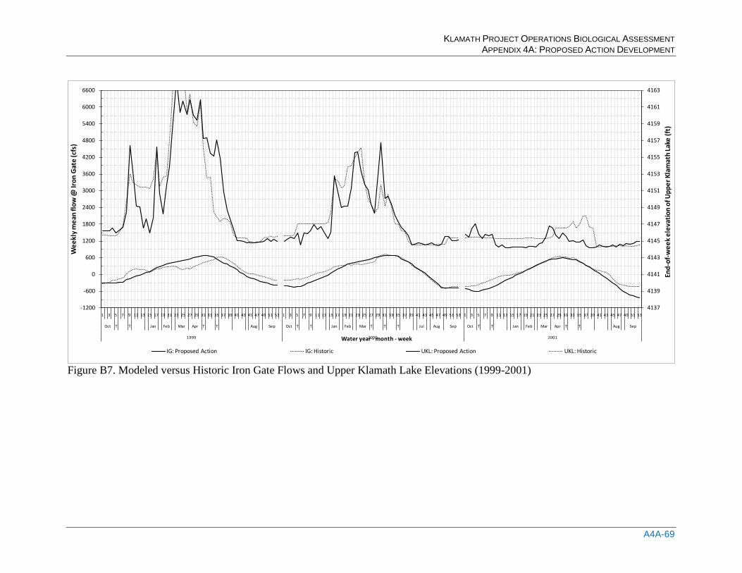
KLAMATH PROJECT OPERATIONS BIOLOGICAL ASSESSMENT APPENDIX 4A: PROPOSED ACTION DEVELOPMENT
A4A-69
4137
4139
4141
4143
4145
4147
4149
4151
4153
4155
4157
4159
4161
4163
-1200
-600
0
600
1200
1800
2400
3000
3600
4200
4800
5400
6000
6600
1 3 5 7 9 11 13 15 17 19 21 23 25 27 29 31 33 35 37 39 41 43 45 47 49 51 53 1 3 5 7 9 11 13 15 17 19 21 23 25 27 29 31 33 35 37 39 41 43 45 47 49 51 53 1 3 5 7 9 11 13 15 17 19 21 23 25 27 29 31 33 35 37 39 41 43 45 47 49 51 53
Oct T T Jan Feb Mar Apr T T Aug Sep Oct T T Jan Feb Mar T T T Jul Aug Sep Oct T T Jan Feb Mar Apr T T Aug Sep
1999 2000 2001
End -
of-w
eek e
leva
tion
of U
pper
Kla
mat
h La
ke (f
t)
Wee
kly m
ean
flow
@ Ir
on G
ate
(cfs
)
Water year - month - week
IG: Proposed Action IG: Historic UKL: Proposed Action UKL: Historic
Figure B7. Modeled versus Historic Iron Gate Flows and Upper Klamath Lake Elevations (1999-2001)
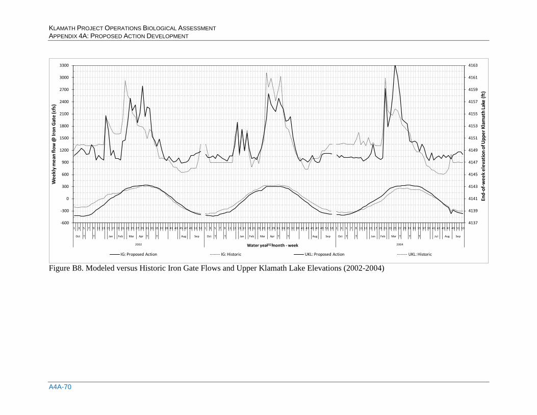
KLAMATH PROJECT OPERATIONS BIOLOGICAL ASSESSMENT APPENDIX 4A: PROPOSED ACTION DEVELOPMENT
A4A-70
4137
4139
4141
4143
4145
4147
4149
4151
4153
4155
4157
4159
4161
4163
-600
-300
0
300
600
900
1200
1500
1800
2100
2400
2700
3000
3300
1 3 5 7 9 11 13 15 17 19 21 23 25 27 29 31 33 35 37 39 41 43 45 47 49 51 53 1 3 5 7 9 11 13 15 17 19 21 23 25 27 29 31 33 35 37 39 41 43 45 47 49 51 53 1 3 5 7 9 11 13 15 17 19 21 23 25 27 29 31 33 35 37 39 41 43 45 47 49 51 53
Oct T T Jan Feb Mar Apr T T Aug Sep Oct T T Jan Feb Mar Apr T T Aug Sep Oct T T Jan Feb Mar T T T Jul Aug Sep
2002 2003 2004
End -
of-w
eek e
leva
tion
of U
pper
Kla
mat
h La
ke (f
t)
Wee
kly m
ean
flow
@ Ir
on G
ate
(cfs
)
Water year - month - week
IG: Proposed Action IG: Historic UKL: Proposed Action UKL: Historic
Figure B8. Modeled versus Historic Iron Gate Flows and Upper Klamath Lake Elevations (2002-2004)
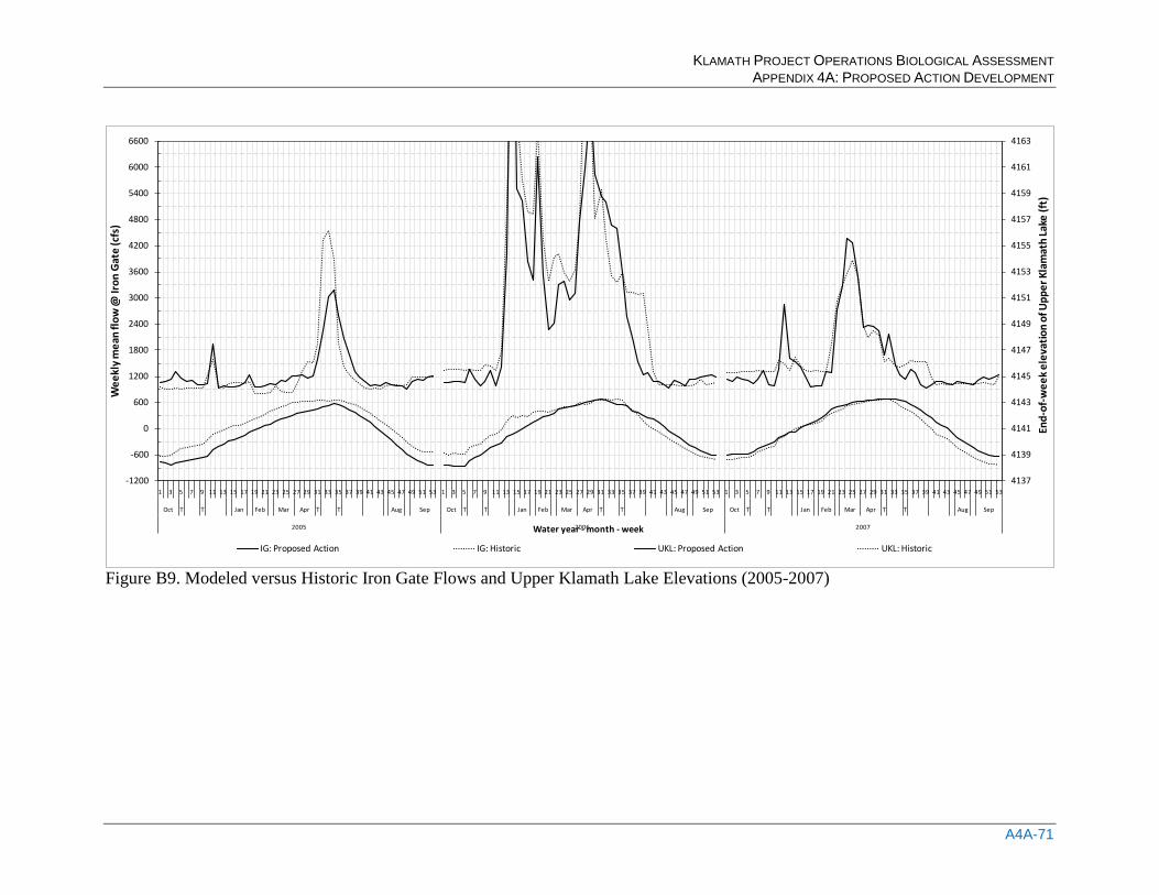
KLAMATH PROJECT OPERATIONS BIOLOGICAL ASSESSMENT APPENDIX 4A: PROPOSED ACTION DEVELOPMENT
A4A-71
4137
4139
4141
4143
4145
4147
4149
4151
4153
4155
4157
4159
4161
4163
-1200
-600
0
600
1200
1800
2400
3000
3600
4200
4800
5400
6000
6600
1 3 5 7 9 11 13 15 17 19 21 23 25 27 29 31 33 35 37 39 41 43 45 47 49 51 53 1 3 5 7 9 11 13 15 17 19 21 23 25 27 29 31 33 35 37 39 41 43 45 47 49 51 53 1 3 5 7 9 11 13 15 17 19 21 23 25 27 29 31 33 35 37 39 41 43 45 47 49 51 53
Oct T T Jan Feb Mar Apr T T Aug Sep Oct T T Jan Feb Mar Apr T T Aug Sep Oct T T Jan Feb Mar Apr T T Aug Sep
2005 2006 2007
End -
of-w
eek e
leva
tion
of U
pper
Kla
mat
h La
ke (f
t)
Wee
kly m
ean
flow
@ Ir
on G
ate
(cfs
)
Water year - month - week
IG: Proposed Action IG: Historic UKL: Proposed Action UKL: Historic
Figure B9. Modeled versus Historic Iron Gate Flows and Upper Klamath Lake Elevations (2005-2007)
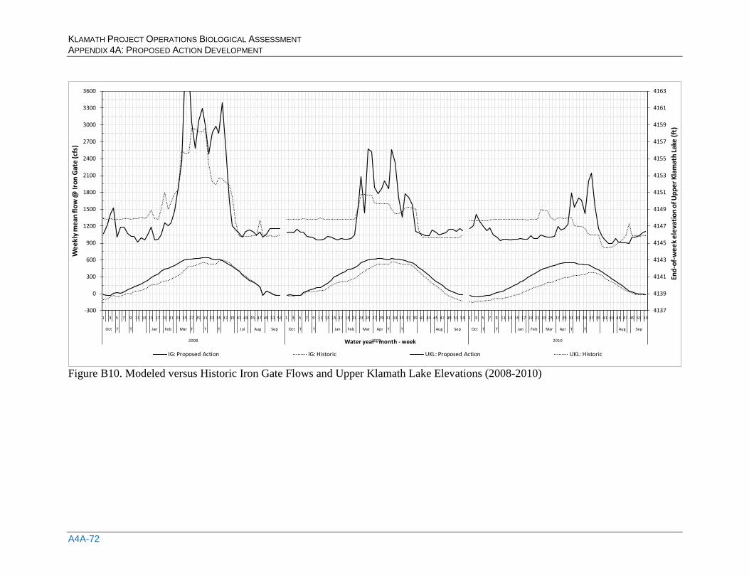
KLAMATH PROJECT OPERATIONS BIOLOGICAL ASSESSMENT APPENDIX 4A: PROPOSED ACTION DEVELOPMENT
A4A-72
4137
4139
4141
4143
4145
4147
4149
4151
4153
4155
4157
4159
4161
4163
-300
0
300
600
900
1200
1500
1800
2100
2400
2700
3000
3300
3600
1 3 5 7 9 11 13 15 17 19 21 23 25 27 29 31 33 35 37 39 41 43 45 47 49 51 53 1 3 5 7 9 11 13 15 17 19 21 23 25 27 29 31 33 35 37 39 41 43 45 47 49 51 53 1 3 5 7 9 11 13 15 17 19 21 23 25 27 29 31 33 35 37 39 41 43 45 47 49 51 53
Oct T T Jan Feb Mar T T T Jul Aug Sep Oct T T Jan Feb Mar Apr T T Aug Sep Oct T T Jan Feb Mar Apr T T Aug Sep
2008 2009 2010
End -
of-w
eek e
leva
tion
of U
pper
Kla
mat
h La
ke (f
t)
Wee
kly m
ean
flow
@ Ir
on G
ate
(cfs
)
Water year - month - week
IG: Proposed Action IG: Historic UKL: Proposed Action UKL: Historic
Figure B10. Modeled versus Historic Iron Gate Flows and Upper Klamath Lake Elevations (2008-2010)
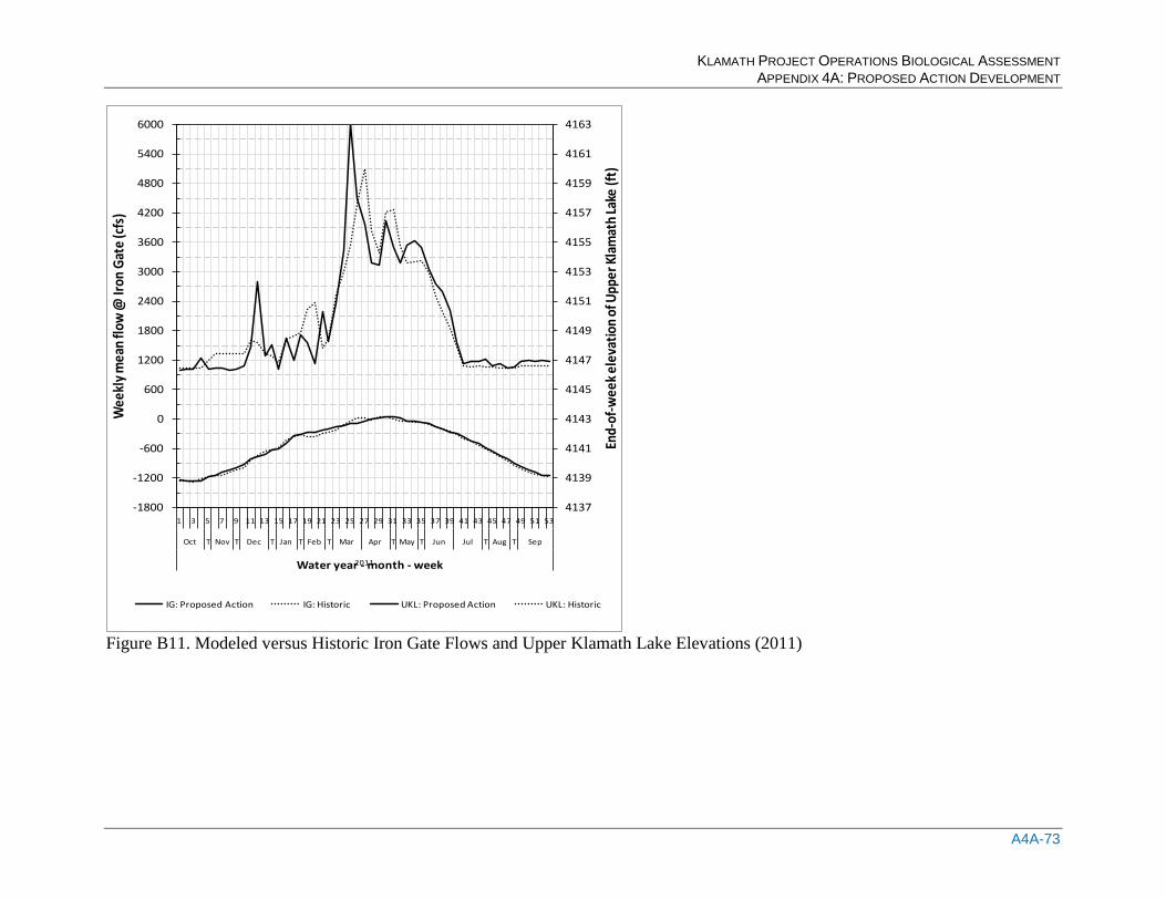
KLAMATH PROJECT OPERATIONS BIOLOGICAL ASSESSMENT APPENDIX 4A: PROPOSED ACTION DEVELOPMENT
A4A-73
4137
4139
4141
4143
4145
4147
4149
4151
4153
4155
4157
4159
4161
4163
-1800
-1200
-600
0
600
1200
1800
2400
3000
3600
4200
4800
5400
6000
1 3 5 7 9 11 13 15 17 19 21 23 25 27 29 31 33 35 37 39 41 43 45 47 49 51 53
Oct T Nov T Dec T Jan T Feb T Mar Apr T May T Jun Jul T Aug T Sep
2011
End-
of-w
eek e
leva
tion o
f Upp
er Kl
amat
h Lak
e (ft
)
Wee
kly m
ean f
low
@ Ir
on G
ate (
cfs)
Water year - month - week
IG: Proposed Action IG: Historic UKL: Proposed Action UKL: Historic
Figure B11. Modeled versus Historic Iron Gate Flows and Upper Klamath Lake Elevations (2011)
KLAMATH PROJECT OPERATIONS BIOLOGICAL ASSESSMENT APPENDIX 4A: PROPOSED ACTION DEVELOPMENT
A4A-74
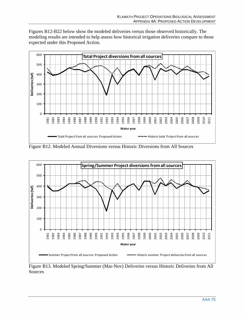
KLAMATH PROJECT OPERATIONS BIOLOGICAL ASSESSMENT APPENDIX 4A: PROPOSED ACTION DEVELOPMENT
A4A-75
Figures B12-B22 below show the modeled deliveries versus those observed historically. The modeling results are intended to help assess how historical irrigation deliveries compare to those expected under this Proposed Action.
0
100
200
300
400
500
600
1981
1982
1983
1984
1985
1986
1987
1988
1989
1990
1991
1992
1993
1994
1995
1996
1997
1998
1999
2000
2001
2002
2003
2004
2005
2006
2007
2008
2009
2010
2011
Deliv
erie
s (ta
f)
Water year
Total Project diversions from all sources
Total Project from all sources: Proposed Action Historic total Project from all sources
Figure B12. Modeled Annual Diversions versus Historic Diversions from All Sources
0
100
200
300
400
500
600
1981
1982
1983
1984
1985
1986
1987
1988
1989
1990
1991
1992
1993
1994
1995
1996
1997
1998
1999
2000
2001
2002
2003
2004
2005
2006
2007
2008
2009
2010
2011
Deliv
erie
s (ta
f)
Water year
Spring/Summer Project diversions from all sources
Summer Project from all sources: Proposed Action Historic summer Project deliveries from all sources
Figure B13. Modeled Spring/Summer (Mar-Nov) Deliveries versus Historic Deliveries from All Sources
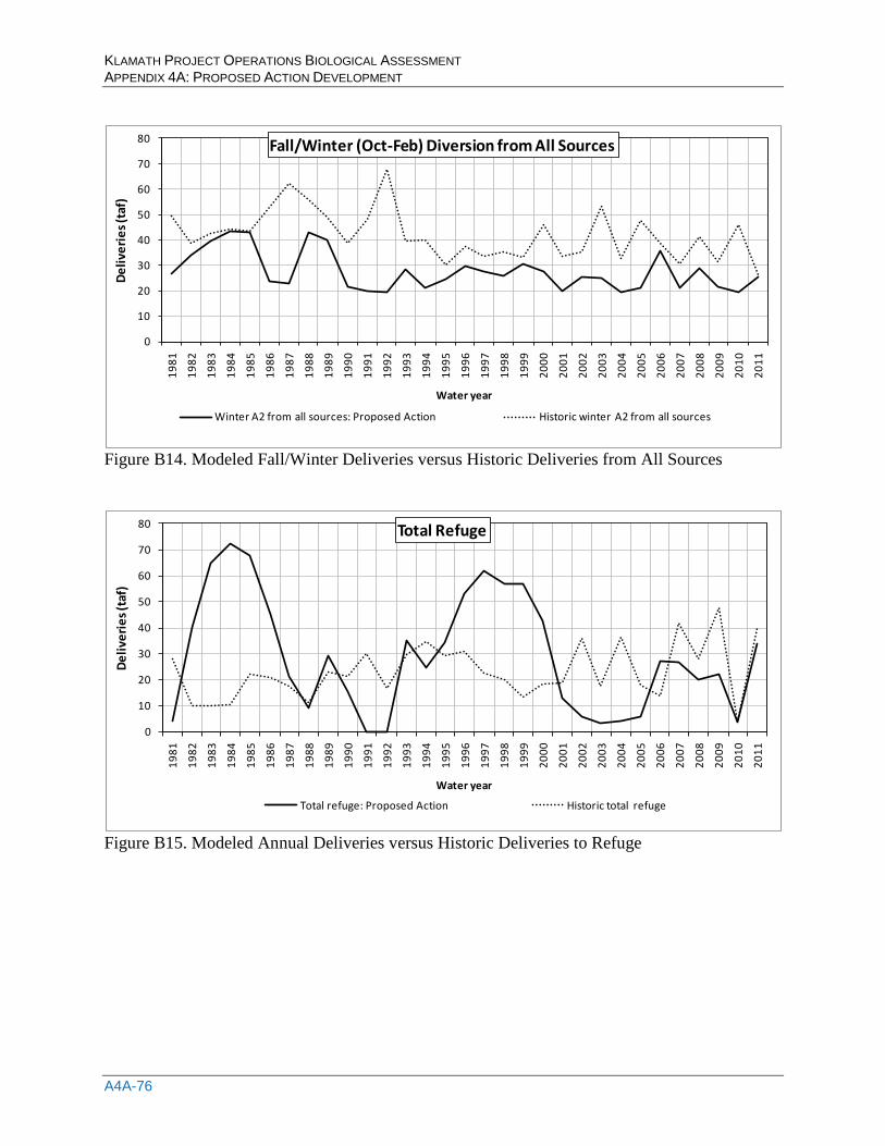
KLAMATH PROJECT OPERATIONS BIOLOGICAL ASSESSMENT APPENDIX 4A: PROPOSED ACTION DEVELOPMENT
A4A-76
0
10
20
30
40
50
60
70
80
1981
1982
1983
1984
1985
1986
1987
1988
1989
1990
1991
1992
1993
1994
1995
1996
1997
1998
1999
2000
2001
2002
2003
2004
2005
2006
2007
2008
2009
2010
2011
Deliv
erie
s (ta
f)
Water year
Fall/Winter (Oct-Feb) Diversion from All Sources
Winter A2 from all sources: Proposed Action Historic winter A2 from all sources
Figure B14. Modeled Fall/Winter Deliveries versus Historic Deliveries from All Sources
0
10
20
30
40
50
60
70
80
1981
1982
1983
1984
1985
1986
1987
1988
1989
1990
1991
1992
1993
1994
1995
1996
1997
1998
1999
2000
2001
2002
2003
2004
2005
2006
2007
2008
2009
2010
2011
Deliv
erie
s (ta
f)
Water year
Total Refuge
Total refuge: Proposed Action Historic total refuge
Figure B15. Modeled Annual Deliveries versus Historic Deliveries to Refuge
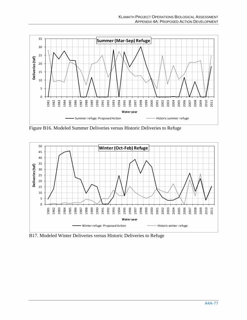
KLAMATH PROJECT OPERATIONS BIOLOGICAL ASSESSMENT APPENDIX 4A: PROPOSED ACTION DEVELOPMENT
A4A-77
0
5
10
15
20
25
30
35
1981
1982
1983
1984
1985
1986
1987
1988
1989
1990
1991
1992
1993
1994
1995
1996
1997
1998
1999
2000
2001
2002
2003
2004
2005
2006
2007
2008
2009
2010
2011
Deliv
erie
s (ta
f)
Water year
Summer (Mar-Sep) Refuge
Summer refuge: Proposed Action Historic summer refuge
Figure B16. Modeled Summer Deliveries versus Historic Deliveries to Refuge
0
5
10
15
20
25
30
35
40
45
50
1981
1982
1983
1984
1985
1986
1987
1988
1989
1990
1991
1992
1993
1994
1995
1996
1997
1998
1999
2000
2001
2002
2003
2004
2005
2006
2007
2008
2009
2010
2011
Deliv
erie
s (ta
f)
Water year
Winter (Oct-Feb) Refuge
Winter refuge: Proposed Action Historic winter refuge
B17. Modeled Winter Deliveries versus Historic Deliveries to Refuge

KLAMATH PROJECT OPERATIONS BIOLOGICAL ASSESSMENT APPENDIX 4A: PROPOSED ACTION DEVELOPMENT
A4A-78
KLAMATH PROJECT OPERATIONS BIOLOGICAL ASSESSMENT APPENDIX 4A: PROPOSED ACTION DEVELOPMENT
A4A-79
Section C: Lower Klamath NWR Historic Deliveries

KLAMATH PROJECT OPERATIONS BIOLOGICAL ASSESSMENT APPENDIX 4A: PROPOSED ACTION DEVELOPMENT
A4A-80
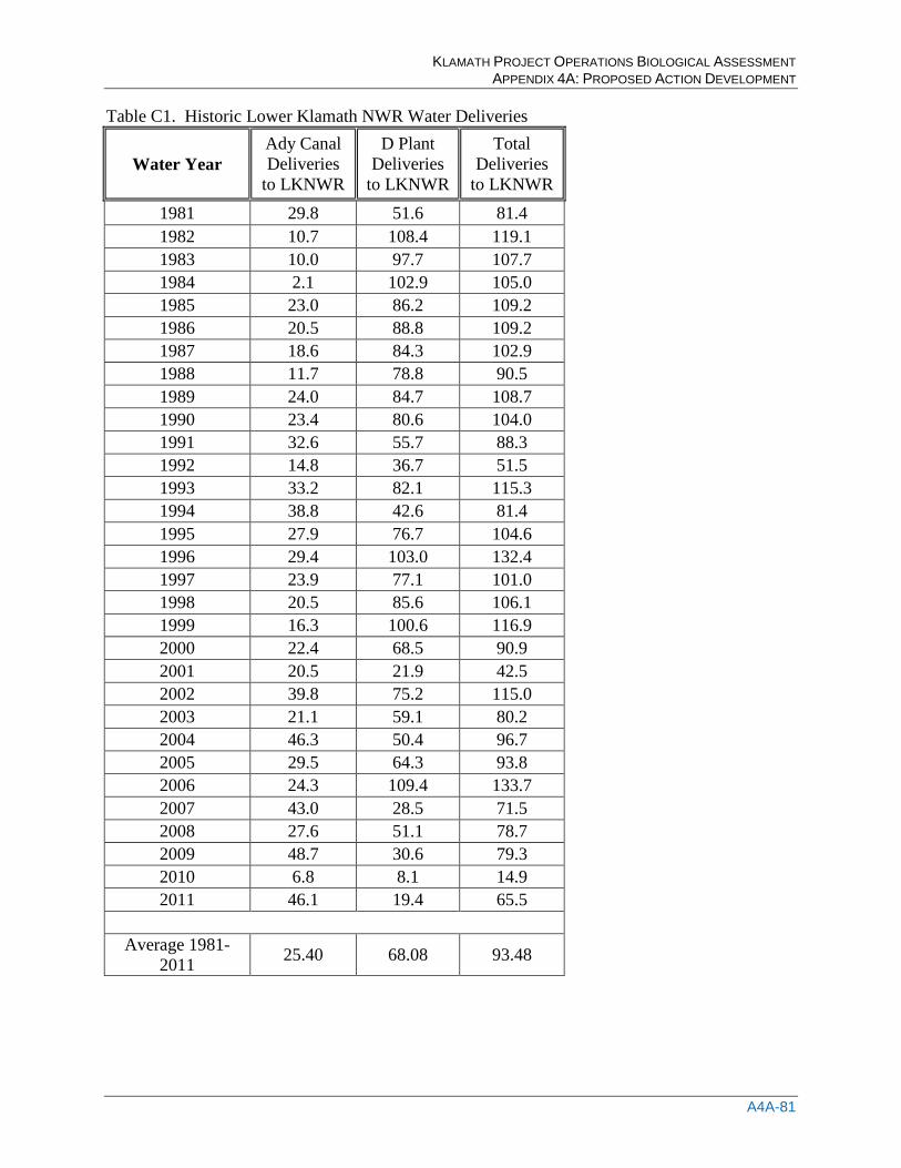
KLAMATH PROJECT OPERATIONS BIOLOGICAL ASSESSMENT APPENDIX 4A: PROPOSED ACTION DEVELOPMENT
A4A-81
Table C1. Historic Lower Klamath NWR Water Deliveries
Water Year Ady Canal Deliveries
to LKNWR
D Plant Deliveries
to LKNWR
Total Deliveries
to LKNWR 1981 29.8 51.6 81.4 1982 10.7 108.4 119.1 1983 10.0 97.7 107.7 1984 2.1 102.9 105.0 1985 23.0 86.2 109.2 1986 20.5 88.8 109.2 1987 18.6 84.3 102.9 1988 11.7 78.8 90.5 1989 24.0 84.7 108.7 1990 23.4 80.6 104.0 1991 32.6 55.7 88.3 1992 14.8 36.7 51.5 1993 33.2 82.1 115.3 1994 38.8 42.6 81.4 1995 27.9 76.7 104.6 1996 29.4 103.0 132.4 1997 23.9 77.1 101.0 1998 20.5 85.6 106.1 1999 16.3 100.6 116.9 2000 22.4 68.5 90.9 2001 20.5 21.9 42.5 2002 39.8 75.2 115.0 2003 21.1 59.1 80.2 2004 46.3 50.4 96.7 2005 29.5 64.3 93.8 2006 24.3 109.4 133.7 2007 43.0 28.5 71.5 2008 27.6 51.1 78.7 2009 48.7 30.6 79.3 2010 6.8 8.1 14.9 2011 46.1 19.4 65.5
Average 1981-
2011 25.40 68.08 93.48
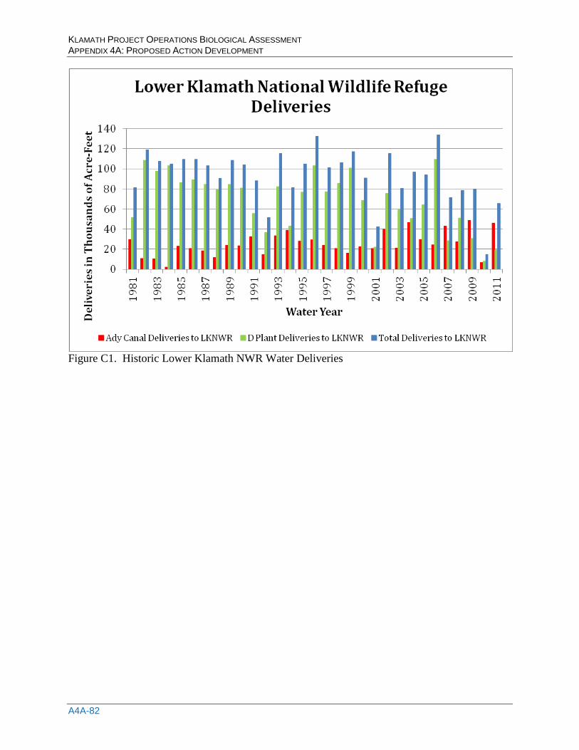
KLAMATH PROJECT OPERATIONS BIOLOGICAL ASSESSMENT APPENDIX 4A: PROPOSED ACTION DEVELOPMENT
A4A-82
Figure C1. Historic Lower Klamath NWR Water Deliveries
KLAMATH PROJECT OPERATIONS BIOLOGICAL ASSESSMENT APPENDIX 4A: PROPOSED ACTION DEVELOPMENT
A4A-83
Section D: Clear Lake and Gerber Water Supply Forecast Models

KLAMATH PROJECT OPERATIONS BIOLOGICAL ASSESSMENT APPENDIX 4A: PROPOSED ACTION DEVELOPMENT
A4A-84
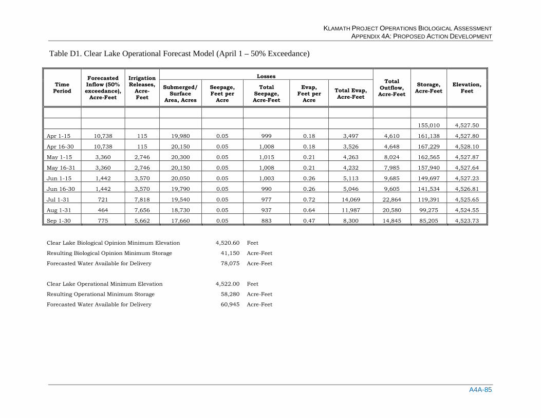
KLAMATH PROJECT OPERATIONS BIOLOGICAL ASSESSMENT APPENDIX 4A: PROPOSED ACTION DEVELOPMENT
A4A-85
Table D1. Clear Lake Operational Forecast Model (April 1 – 50% Exceedance)
Time Period
Forecasted Inflow (50% exceedance),
Acre-Feet
Irrigation Releases,
Acre-Feet
Losses Total
Outflow, Acre-Feet
Storage, Acre-Feet
Elevation, Feet
Submerged/ Surface
Area, Acres
Seepage, Feet per
Acre
Total Seepage, Acre-Feet
Evap, Feet per
Acre
Total Evap, Acre-Feet
155,010 4,527.50
Apr 1-15 10,738 115 19,980 0.05 999 0.18 3,497 4,610 161,138 4,527.80
Apr 16-30 10,738 115 20,150 0.05 1,008 0.18 3,526 4,648 167,229 4,528.10
May 1-15 3,360 2,746 20,300 0.05 1,015 0.21 4,263 8,024 162,565 4,527.87
May 16-31 3,360 2,746 20,150 0.05 1,008 0.21 4,232 7,985 157,940 4,527.64
Jun 1-15 1,442 3,570 20,050 0.05 1,003 0.26 5,113 9,685 149,697 4,527.23
Jun 16-30 1,442 3,570 19,790 0.05 990 0.26 5,046 9,605 141,534 4,526.81
Jul 1-31 721 7,818 19,540 0.05 977 0.72 14,069 22,864 119,391 4,525.65
Aug 1-31 464 7,656 18,730 0.05 937 0.64 11,987 20,580 99,275 4,524.55
Sep 1-30 775 5,662 17,660 0.05 883 0.47 8,300 14,845 85,205 4,523.73
Clear Lake Biological Opinion Minimum Elevation 4,520.60 Feet
Resulting Biological Opinion Minimum Storage 41,150 Acre-Feet
Forecasted Water Available for Delivery 78,075 Acre-Feet
Clear Lake Operational Minimum Elevation 4,522.00 Feet
Resulting Operational Minimum Storage 58,280 Acre-Feet
Forecasted Water Available for Delivery 60,945 Acre-Feet
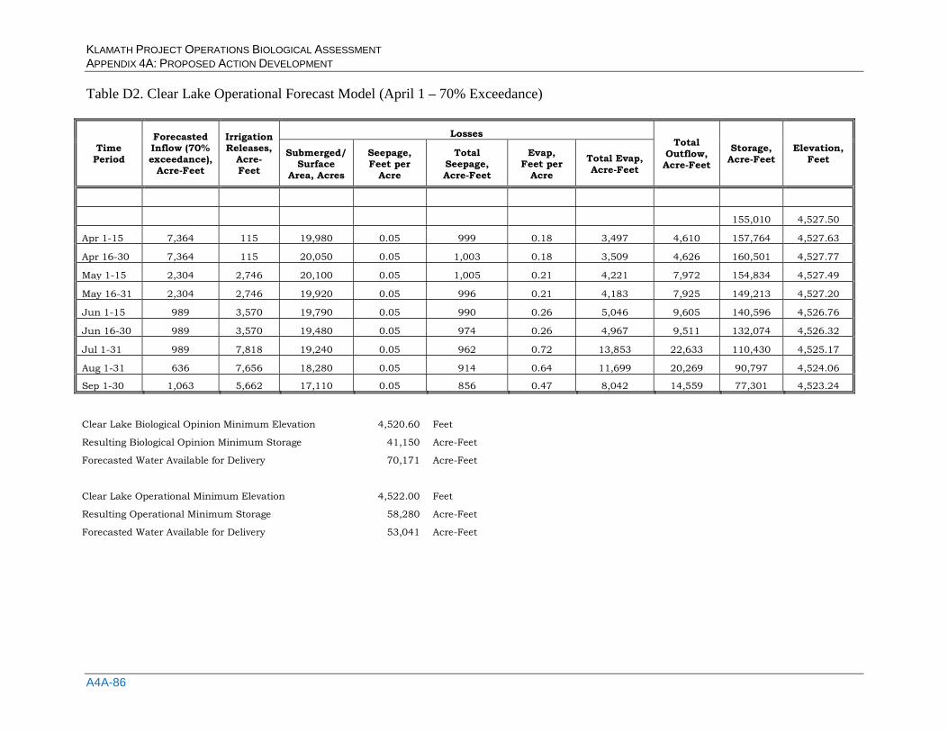
KLAMATH PROJECT OPERATIONS BIOLOGICAL ASSESSMENT APPENDIX 4A: PROPOSED ACTION DEVELOPMENT
A4A-86
Table D2. Clear Lake Operational Forecast Model (April 1 – 70% Exceedance)
Time Period
Forecasted Inflow (70% exceedance),
Acre-Feet
Irrigation Releases,
Acre-Feet
Losses Total
Outflow, Acre-Feet
Storage, Acre-Feet
Elevation, Feet
Submerged/ Surface
Area, Acres
Seepage, Feet per
Acre
Total Seepage, Acre-Feet
Evap, Feet per
Acre
Total Evap, Acre-Feet
155,010 4,527.50
Apr 1-15 7,364 115 19,980 0.05 999 0.18 3,497 4,610 157,764 4,527.63
Apr 16-30 7,364 115 20,050 0.05 1,003 0.18 3,509 4,626 160,501 4,527.77
May 1-15 2,304 2,746 20,100 0.05 1,005 0.21 4,221 7,972 154,834 4,527.49
May 16-31 2,304 2,746 19,920 0.05 996 0.21 4,183 7,925 149,213 4,527.20
Jun 1-15 989 3,570 19,790 0.05 990 0.26 5,046 9,605 140,596 4,526.76
Jun 16-30 989 3,570 19,480 0.05 974 0.26 4,967 9,511 132,074 4,526.32
Jul 1-31 989 7,818 19,240 0.05 962 0.72 13,853 22,633 110,430 4,525.17
Aug 1-31 636 7,656 18,280 0.05 914 0.64 11,699 20,269 90,797 4,524.06
Sep 1-30 1,063 5,662 17,110 0.05 856 0.47 8,042 14,559 77,301 4,523.24
Clear Lake Biological Opinion Minimum Elevation 4,520.60 Feet
Resulting Biological Opinion Minimum Storage 41,150 Acre-Feet
Forecasted Water Available for Delivery 70,171 Acre-Feet
Clear Lake Operational Minimum Elevation 4,522.00 Feet
Resulting Operational Minimum Storage 58,280 Acre-Feet
Forecasted Water Available for Delivery 53,041 Acre-Feet
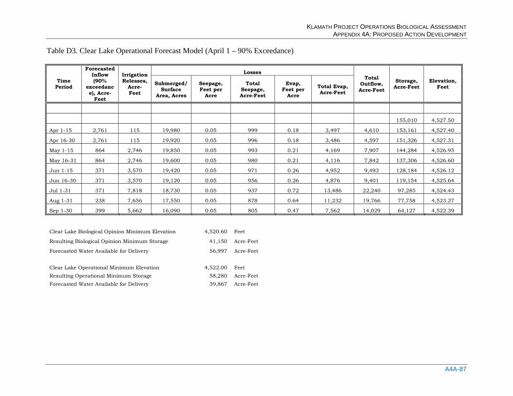
KLAMATH PROJECT OPERATIONS BIOLOGICAL ASSESSMENT APPENDIX 4A: PROPOSED ACTION DEVELOPMENT
A4A-87
Table D3. Clear Lake Operational Forecast Model (April 1 – 90% Exceedance)
Time Period
Forecasted Inflow (90%
exceedance), Acre-
Feet
Irrigation Releases,
Acre-Feet
Losses Total
Outflow, Acre-Feet
Storage, Acre-Feet
Elevation, Feet Submerged/
Surface Area, Acres
Seepage, Feet per
Acre
Total Seepage, Acre-Feet
Evap, Feet per
Acre
Total Evap, Acre-Feet
155,010 4,527.50
Apr 1-15 2,761 115 19,980 0.05 999 0.18 3,497 4,610 153,161 4,527.40
Apr 16-30 2,761 115 19,920 0.05 996 0.18 3,486 4,597 151,326 4,527.31
May 1-15 864 2,746 19,850 0.05 993 0.21 4,169 7,907 144,284 4,526.95
May 16-31 864 2,746 19,600 0.05 980 0.21 4,116 7,842 137,306 4,526.60
Jun 1-15 371 3,570 19,420 0.05 971 0.26 4,952 9,493 128,184 4,526.12
Jun 16-30 371 3,570 19,120 0.05 956 0.26 4,876 9,401 119,154 4,525.64
Jul 1-31 371 7,818 18,730 0.05 937 0.72 13,486 22,240 97,285 4,524.43
Aug 1-31 238 7,656 17,550 0.05 878 0.64 11,232 19,766 77,758 4,523.27
Sep 1-30 399 5,662 16,090 0.05 805 0.47 7,562 14,029 64,127 4,522.39
Clear Lake Biological Opinion Minimum Elevation 4,520.60 Feet
Resulting Biological Opinion Minimum Storage 41,150 Acre-Feet
Forecasted Water Available for Delivery 56,997 Acre-Feet
Clear Lake Operational Minimum Elevation 4,522.00 Feet
Resulting Operational Minimum Storage 58,280 Acre-Feet Forecasted Water Available for Delivery 39,867 Acre-Feet
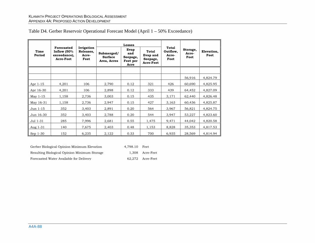
KLAMATH PROJECT OPERATIONS BIOLOGICAL ASSESSMENT APPENDIX 4A: PROPOSED ACTION DEVELOPMENT
A4A-88
Table D4. Gerber Reservoir Operational Forecast Model (April 1 – 50% Exceedance)
Time Period
Forecasted Inflow (50% exceedance),
Acre-Feet
Irrigation Releases,
Acre-Feet
Losses Total
Outflow, Acre-Feet
Storage, Acre-Feet
Elevation, Feet Submerged/
Surface Area, Acres
Evap and
Seepage, Feet per
Acre
Total Evap and Seepage, Acre-Feet
56,916 4,824.79
Apr 1-15 4,201 106 2,790 0.12 321 426 60,690 4,825.95
Apr 16-30 4,201 106 2,898 0.12 333 439 64,452 4,827.09
May 1-15 1,158 2,736 3,003 0.15 435 3,171 62,440 4,826.48
May 16-31 1,158 2,736 2,947 0.15 427 3,163 60,436 4,825.87
Jun 1-15 352 3,403 2,891 0.20 564 3,967 56,821 4,824.75
Jun 16-30 352 3,403 2,788 0.20 544 3,947 53,227 4,823.60
Jul 1-31 285 7,996 2,681 0.55 1,475 9,471 44,042 4,820.58
Aug 1-31 140 7,675 2,403 0.48 1,153 8,828 35,353 4,817.53
Sep 1-30 152 6,235 2,122 0.33 700 6,935 28,569 4,814.94
Gerber Biological Opinion Minimum Elevation 4,798.10 Feet
Resulting Biological Opinion Minimum Storage 1,308 Acre-Feet
Forecasted Water Available for Delivery 62,272 Acre-Feet
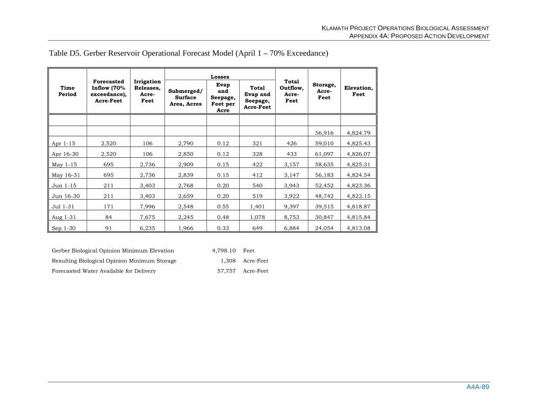
KLAMATH PROJECT OPERATIONS BIOLOGICAL ASSESSMENT APPENDIX 4A: PROPOSED ACTION DEVELOPMENT
A4A-89
Table D5. Gerber Reservoir Operational Forecast Model (April 1 – 70% Exceedance)
Time Period
Forecasted Inflow (70% exceedance),
Acre-Feet
Irrigation Releases,
Acre-Feet
Losses Total
Outflow, Acre-Feet
Storage, Acre-Feet
Elevation, Feet Submerged/
Surface Area, Acres
Evap and
Seepage, Feet per
Acre
Total Evap and Seepage, Acre-Feet
56,916 4,824.79
Apr 1-15 2,520 106 2,790 0.12 321 426 59,010 4,825.43
Apr 16-30 2,520 106 2,850 0.12 328 433 61,097 4,826.07
May 1-15 695 2,736 2,909 0.15 422 3,157 58,635 4,825.31
May 16-31 695 2,736 2,839 0.15 412 3,147 56,183 4,824.54
Jun 1-15 211 3,403 2,768 0.20 540 3,943 52,452 4,823.36
Jun 16-30 211 3,403 2,659 0.20 519 3,922 48,742 4,822.15
Jul 1-31 171 7,996 2,548 0.55 1,401 9,397 39,515 4,818.87
Aug 1-31 84 7,675 2,245 0.48 1,078 8,753 30,847 4,815.84
Sep 1-30 91 6,235 1,966 0.33 649 6,884 24,054 4,813.08
Gerber Biological Opinion Minimum Elevation 4,798.10 Feet Resulting Biological Opinion Minimum Storage 1,308 Acre-Feet Forecasted Water Available for Delivery 57,757 Acre-Feet
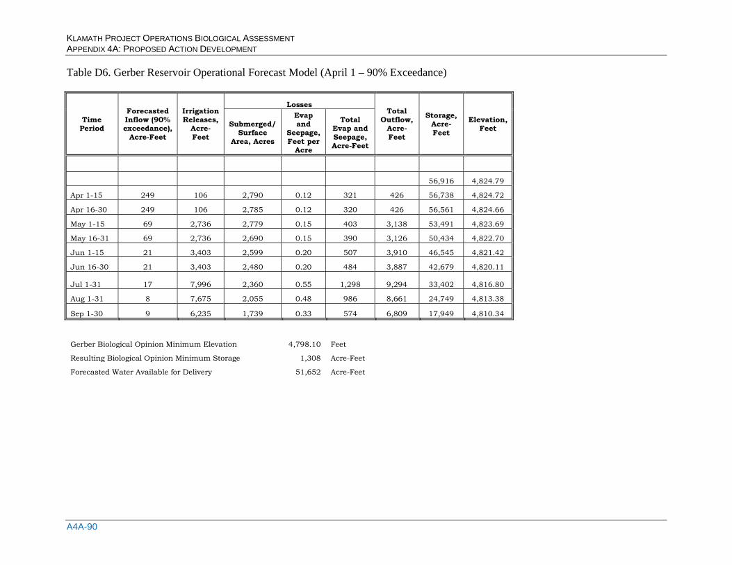
KLAMATH PROJECT OPERATIONS BIOLOGICAL ASSESSMENT APPENDIX 4A: PROPOSED ACTION DEVELOPMENT
A4A-90
Table D6. Gerber Reservoir Operational Forecast Model (April 1 – 90% Exceedance)
Time Period
Forecasted Inflow (90% exceedance),
Acre-Feet
Irrigation Releases,
Acre-Feet
Losses Total
Outflow, Acre-Feet
Storage, Acre-Feet
Elevation, Feet Submerged/
Surface Area, Acres
Evap and
Seepage, Feet per
Acre
Total Evap and Seepage, Acre-Feet
56,916 4,824.79
Apr 1-15 249 106 2,790 0.12 321 426 56,738 4,824.72
Apr 16-30 249 106 2,785 0.12 320 426 56,561 4,824.66
May 1-15 69 2,736 2,779 0.15 403 3,138 53,491 4,823.69
May 16-31 69 2,736 2,690 0.15 390 3,126 50,434 4,822.70
Jun 1-15 21 3,403 2,599 0.20 507 3,910 46,545 4,821.42
Jun 16-30 21 3,403 2,480 0.20 484 3,887 42,679 4,820.11
Jul 1-31 17 7,996 2,360 0.55 1,298 9,294 33,402 4,816.80
Aug 1-31 8 7,675 2,055 0.48 986 8,661 24,749 4,813.38
Sep 1-30 9 6,235 1,739 0.33 574 6,809 17,949 4,810.34
Gerber Biological Opinion Minimum Elevation 4,798.10 Feet Resulting Biological Opinion Minimum Storage 1,308 Acre-Feet Forecasted Water Available for Delivery 51,652 Acre-Feet

KLAMATH PROJECT OPERATIONS BIOLOGICAL ASSESSMENT APPENDIX 4B: EXAMPLE: PLAN TO RELOCATE TULE LAKE SUCKERS
Appendix 4B: Example: Plan to Relocate Tule
Lake Suckers

KLAMATH PROJECT OPERATIONS BIOLOGICAL ASSESSMENT APPENDIX 4B: EXAMPLE: PLAN TO RELOCATE TULE LAKE SUCKERS
KLAMATH PROJECT OPERATIONS BIOLOGICAL ASSESSMENT APPENDIX 4B: EXAMPLE: PLAN TO RELOCATE TULE LAKE SUCKERS
A4B-1
Example: Tule Lake (Siskiyou County) California Adult Sucker Relocation
Background
Currently, Tule Lake in northern Siskiyou County, California, is the remnant of a larger lake by
the same name. Tule Lake (both Sumps 1A and 1B), Tule Lake National Wildlife Refuge and
surrounding private agricultural lands occupy the historic lake bed of the original Tule Lake
(approximately 95,000 acres) in both California and Oregon. Presently Tule Lake consists of
approximately 10,500 acres of shallow open water (Sump 1A, 6,500 acres, 0.25-4.0 ft depth;
Sump 1B, 3,500 acres, 2.0-4.0 ft depth). Studies indicate that adult suckers primarily reside in
Sump 1A of Tule Lake during spring, summer and fall months (Hicks et al. 1999, Beckstrand et
al. 2000). Both Klamath Basin ESA-listed sucker species (Lost River suckers, Deltistes luxatus;
shortnose suckers, Chasmistes brevirostris) currently inhabit Tule Lake and may number in the
several hundreds to thousands (Scoppettone et al. 1995, Hodge 2007, 2008, Hodge and Buettner
2009).
Historically Tule Lake was fed by flow from the Lost River and overflow from the upper
Klamath River; however, Clear Lake was dammed early in the 20th
Century to reduce flows in
the Lost River, and any substantial accretions in the Lost River are now diverted to the Klamath
River, and the only water flowing to Tule Lake from the Klamath River now is for agriculture.
As a result, inflows to Tule Lake are primarily the result of agricultural returns from groundwater
and surface water from Upper Klamath Lake. Because of low reservoir levels and substantially-
reduced deliveries to agriculture as a result of drought, Reclamation is likely unable to maintain a
minimum elevation of 4034.6 ft. Because evaporative losses from Tule Lake are likely to exceed
3 feet through the summer, maximum water depths are anticipated to be no more than 1-2 feet by
the end of summer. Concerns are that with these shallow depths, suckers will be highly
vulnerable to white pelican predation, poor water quality, and masses of filamentous algae.
Given the likelihood of Tule Lake surface elevation dropping to a level that may compromise
sucker health and survival, an effort to salvage adult suckers from Tule Lake is planned in the
spring of 2010 prior to water temperature becoming too high (greater than 15º C) or the lake
elevation becoming too low. Salvaged adult suckers will be handled and transported consistent
with Sucker Handling Guidelines for Klamath Basin Suckers (Reclamation, October 2008;
Appendix 1).
Potential relocation sites for the salvaged suckers include Upper Klamath Lake, Clear Lake, and
Gerber Reservoir. Clear Lake has several advantages because it is in the same watershed as Tule
Lake and is in California, which makes permitting easier. The primary disadvantages to Clear
Lake Reservoir are its distance over remote, poorly maintained roads and it is a shallow lake that
may also be influenced by drought conditions. Gerber Reservoir is within the same watershed as
Tule Lake on the Oregon side which makes permitting a potential problem (i.e., transport of fish
across state lines). A possible advantage of moving some Lost River suckers to Gerber is that if a
new self-sustaining population could be established it may benefit recovery. However, Gerber is
relatively small and lake levels there are also influenced by drought conditions. Upper Klamath
Lake is perhaps the best relocation option for the fish. Although Upper Klamath Lake is
relatively low this year, it has the most habitat of any of the upper basin lakes with sucker
populations. Disadvantages of Upper Klamath Lake are that it is both in a different state, making
permitting more complex, and it is in a different subbasin. Although Tule Lake and Upper
KLAMATH PROJECT OPERATIONS BIOLOGICAL ASSESSMENT APPENDIX 4B: EXAMPLE: PLAN TO RELOCATE TULE LAKE SUCKERS
A4B-2
Klamath Lake are in different subbasins, most of the water reaching Tule Lake is from Upper
Klamath Lake that passes through the Klamath Project canals. Previous discussions with the
Oregon Department of Fish and Wildlife indicate that under extreme circumstances they will
consider out of basin and across state line transfers of endangered suckers.
Anticipated Tule Lake depths are 1 to 1.5 m during relocation efforts in March through June.
The shallowest area of water likely to be encountered is within 100 m of the Tule Lake boat
launch off Hill Road. Shallow draft boats (e.g., jon or utility boats, etc) with propeller motors
are sufficient at lake elevations expected during these months.
Objective
To relocate adult suckers from Tule Lake to a more stable environment within the historic range
of Klamath Basin sucker species (i.e., Upper Klamath Lake, Oregon, or Clear Lake, California)
prior to a surface elevation drop in Tule Lake that may compromise sucker survival. By-catch
species will be released into Tule Lake upon capture.
Methods
To be consistent with Reclamation’s permits or Biological Opinion for ESA-listed suckers. The
following method is recommended, but other methods in conjunction with the primary method
below will be equally considered.
Many standard fish sampling gear can be employed to effectively capture adult suckers. The
preferred method is using 300 ft length trammel nets with 1.5 inch bar mesh on the inside
(primary) panel and 12 inch mesh on both of the outside panels. This method has proven safe
and effective for capture of adult suckers during other fish studies in the Upper Klamath Basin.
Trammel nets will be inspected for entangled fish approximately once an hour. Non-target fish
species will be released at the point of capture. Captured adult suckers will be removed from
nets and held in aerated live-wells aboard the capture boat while net inspections are conducted
and before transfer to land-based transport. Ferrying captured suckers to land-based transport
should occur between inspections of nets to ensure that fish are held no longer than necessary.
Other methods, such as long-handled dipnets, seines or electro-fishing, may be considered and
employed if there is indication the method may be effective to capture adult suckers (e.g.,
concentrated fish in a small area).
Ideally adult sucker capture, handling and transport will occur before water temperatures in Tule
Lake reach 15 ºC. While water temperatures are below 15º C, each captured fish should be
identified to species and sex, measured for fork length (mm), and implanted near the pelvic
girdle with a passive integrated transponder (PIT) tag via a large gauge needle and plunger.
Species, sex, length and PIT tag serial will be recorded for adult suckers. When water
temperatures are between 15 and 20º C, fish salvage will continue but handling times will be
reduced through the elimination of identifying sex, measuring length, and PIT tagging. Thus,
water temperature in Tule Lake is an important aspect of this plan and will be monitored closely.
Captured adult suckers will be held in aerated live-wells while aboard the capture boat. Fish will
be routinely transported from the netting locations on Tule Lake to land-based transport
approximately every hour. Fish will be transferred from boat live-wells to larger aerated live-
wells (approximately 200 gallon) for land-based transport. Large live-wells are constructed to fit
KLAMATH PROJECT OPERATIONS BIOLOGICAL ASSESSMENT APPENDIX 4B: EXAMPLE: PLAN TO RELOCATE TULE LAKE SUCKERS
A4B-3
in the open bed of a standard pickup truck or on a trailer and will be filled to 80% capacity
(about 160 gallons) of well water or domestic water that has been treated to remove chlorination.
Fish will be transported in these large live-wells to approved release sites on Upper Klamath
Lake (or Clear Lake) in a manner consistent with Sucker Handling Guidelines for Klamath Basin
Suckers (Reclamation October 2008; Appendix 1). Temperature and dissolved oxygen should be
monitored during transport. Water temperature in live-wells may need tempering with ice when
temperatures exceed 15-16º C.
Transport crews may consist of one or two crewmembers to transfer fish between live-wells,
maintain aeration equipment, monitor water temperature, stocking densities and dissolved
oxygen in live-wells, and driving vehicles to release sites. Release of captured fish, dependent
upon the live-well used, can either occur as release of water and fish from the live-well down a
rigid slide into release waters or as a transfer of fish from the live-well to release waters using a
dipnet. If water and fish are simultaneously released, then drivers will replenish the transport
live-wells with water (well or treated domestic supply) before returning to the Tule Lake boat
launch area. Two or three transport crews will work in unison with two or three capture crews
during the primary adult sucker salvage effort so that transportation of fish is a continuous
process.
All fish will be released at sites with more permanent water. Upper Klamath Lake is likely the
primary release site. Final release sites will be decided upon through conferencing with Oregon
Department of Fish and Wildlife, California Department of Fish and Game, the Klamath Tribes,
and U.S. Fish and Wildlife Service. Boat ramp release sites on Upper Klamath Lake and Clear
Lake should be considered within the proposal. Potential (but not all) release sites include:
A. Moore Park in Klamath Falls – 32 miles, 50 minutes
B. Howard Bay off Highway 140 – 38 miles, 50 minutes
C. Hagelstein County Park off Highway 97 – 40 miles, 60 minutes
D. Shoalwater Bay (Eagle Ridge County Park) –50 miles, 75 minutes
E. Modoc Point unimproved boat launch – 44 miles, 60 minutes
F. Williamson River Delta Nature Conservancy boat launch – 53 miles, 75 minutes
G. Pelican Bay, 60 miles, 80 minutes
H. Odessa Creek unimproved boat launch, 51 miles, 75 minutes
I. Harriman Springs (near Pelican Bay), 60 miles, 80 minutes
J. The only stable-environment, release site in California within the historic range of both
Lost River and shortnose suckers are unimproved boat launches on the west lobe and east
lobe of Clear Lake Reservoir via forest service roads off Highway 39/139 about 35 miles
and 120 minutes from Tule Lake Sump 1A.
KLAMATH PROJECT OPERATIONS BIOLOGICAL ASSESSMENT APPENDIX 4B: EXAMPLE: PLAN TO RELOCATE TULE LAKE SUCKERS
A4B-4
Equipment Needs -Minimum of two capture crews (two-person crew working from shallow draft boats), and two
land-based transportation crews (one- or two-person crew transporting suckers from Tule Lake to
a release site).
-Two land-based transportation vehicles suitable for water tanks.
-Two watercraft suitable for shallow water operation.
-Fish handling equipment to include fish measuring boards, temporary floating net pens, dip nets,
electrofishers, trammel nets, seines, PIT tagging equipment and tags.
Deliverables
A summary report will include a measure of effort and captured fish. The summary report
should include water temperatures (i.e., natural bodies of water and transport live-wells) during
transport and the additional data gathered from adult suckers while water temperatures permit the
data collection (i.e., fork lengths, species, sex, and PIT tag serials on individual adult suckers).
A draft summary report is anticipated within 60 days of concluding fish relocation effort.
Literature Cited
Beckstrand, J., D.M. Mauser, D. Thomson, and L.A. Hicks. 2000. Ecology of shortnose and Lost
River suckers in Tule Lake National Wildlife Refuge, California, Progress report #2, February –
December, 2000. 55p.
Hicks, L.A., D.M. Mauser, J. Beckstrand, and D. Thomson. 1999. Ecology of shortnose and Lost
River suckers in Tule Lake National Wildlife Refuge, California, Progress Report, April –
November 1999. 39p.
Hodge, J. 2007. 2006 sucker spawning in the lower Lost River, Oregon. Unpublished report.
U.S. Fish and Wildlife Service, Klamath Falls Fish and Wildlife Office, Oregon. March 23,
2007. 18 p.
Hodge, J. 2008. Sucker population monitoring in Tule Lake and Lower Lost River, Oregon and
California. Unpublished report. U.S. Fish and Wildlife Service, Klamath Falls Fish and Wildlife
Office, Oregon.
Hodge, J. and M. Buettner. 2009. Sucker population monitoring in Tule Lake and Lower Lost
River, 2006-2008. Unpublished report. U.S. Fish and Wildlife Service, Klamath Falls Fish and
Wildlife Office, Oregon.
KLAMATH PROJECT OPERATIONS BIOLOGICAL ASSESSMENT APPENDIX 4B: EXAMPLE: PLAN TO RELOCATE TULE LAKE SUCKERS
A4B-5
Appendix I. Sucker Handling Guidelines for Klamath Basin Suckers
Handling Guidelines for Klamath Basin Suckers Reclamation, Klamath Basin Area Office
October 2008
Background
Reclamation has annually salvaged fish from throughout the Klamath Project canals since 1991.
A reduced canal salvage effort was implemented following approval by USFWS with the
construction and operation of the fish screens at A Canal and Clear Lake Dam in 2003. Much of
Reclamation’s past fish salvage efforts in Project canals has been conducted using electrofishing
techniques.
Reclamation staff will continue to salvage suckers from Project canals following the dewatering
of canals each autumn. Reclamation has prepared a salvage plan for the period 2008-2010.
Reclamation proposes in that salvage plan to handle both salvage and trap and haul fish in
manner that may improve survivorship of these fish. While Reclamation staff is committed to
understanding the impact of electrofishing on juvenile suckers, this document is intended as
guidance on how fish are handled after capture. If there is reason to suspect electrofishing results
in significant injuries to juvenile suckers, then Reclamation will explore other techniques to
capture fish to be salvaged.
The high pathogen/parasite loads of juvenile suckers in 2006 and 2007 from the Link River and J
Canal of the Lost River system suggest that sucker survival may be impaired even when captured
from and returned to natural environments of the Klamath Basin (Banner 2006, Banner and
Stocking 2006, Banner 2007). Although there is evidence that juvenile sucker health may be
impaired, surviving larval (early juvenile) suckers held at the A Canal in late summer 2007 only
experienced episodic parasite infections that were characterized as ‘mild’ (Foott et al. 2007). The
authors did not observe signs of disease due to either bacteria or external parasites, but did note
internal bacterial flora was consistent while external parasites did change in species composition
throughout the study. In contrast, bacteria (e.g., Flavobacteria columnare and Aeromonas
hydrophila) have been associated with adult sucker losses in Upper Klamath Lake (Perkins et al.
2000, Cipriano et al. 2007).
The principal objective of both salvage effort and trap and haul activity is to return fish to
environments in a manner that may improve individual survival. To improve health of salvaged
suckers, Reclamation proposes to hold and transport them in saline solution at the concentrations
listed below. The purpose of the saline solution is to improve osmoregulation and respiration of
transported fish while in-transit. Furthermore, the use of saline solution during transport may
also combat some of the external parasites common on fishes from Upper Klamath Lake (Foott
2004, Foott et al. 2007). The saline solution will only be mixed with un-chlorinated well water.
Aeration will be provided through pressurized atmospheric air. A commercially available slime
coat will be added to each tank. These measures should improve fish respiration during transport.
Reclamation proposes the following guidelines for safe fish handling after capture during both
salvage and trap and haul activities for the period of 2008 through 2010. Reclamation will work
KLAMATH PROJECT OPERATIONS BIOLOGICAL ASSESSMENT APPENDIX 4B: EXAMPLE: PLAN TO RELOCATE TULE LAKE SUCKERS
A4B-6
with Dr. Scott Foott of USFWS, California-Nevada Fish Health Center, to evaluate the short-
term sucker survivorship following both salvage and trap and haul. Reclamation and Dr. Foott
will also collaborate to explore other options intended to increase survivorship of relocated
suckers. This work is separate from the fish handling guidelines presented here. Reclamation
proposes that biologists from USFWS and Reclamation discuss and consider revisions to these
guidelines annually although this document is intended to be in use from 2008 through 2010
without revision. Reclamation will use a disinfectant, such as Virkon Aquatic (Western
Chemical, Inc.; www.wchemical.com), to prevent spread of aquatic species or disease.
Holding of Klamath Basin Suckers
Immediate upon capture, suckers will be held in easily transported totes that contain a 0.5%
saline solution of well water. When possible, aeration will be provided to these totes via an
airstone and pressurized atmospheric air. These fish will be transferred to larger transport tanks
following measurement and the above procedures will able for large or small transport tanks.
As of October 2008, Reclamation does not propose to hold adult or juvenile suckers beyond a
period that is considered necessary before transporting and releasing. The holding of suckers for
a 5 day period is only to maximize the efficiency of transport and release of suckers. During the
trap and haul efforts, Reclamation will collect juvenile suckers from the A Canal fish bypass
and/or the Link River for transport and release in the northern portion of Upper Klamath Lake.
We propose to transport juvenile suckers once at the end of each week during trap and haul
efforts. More frequent trips may be necessary if the number of juvenile suckers captured
surpasses our capabilities to hold fish at the Fish Evaluation Station (FES). Reclamation
approximates our fish-holding facilities at 200 to 1,000 juvenile suckers, dependent upon size of
the juveniles. As a general rule, juvenile suckers will be transported for release when we have
100 individuals in holding and every Friday regardless of the number of fish. Fish will be held by
Reclamation at the FES in a flow-through system with water from Upper Klamath Lake. If poor
water quality conditions at the FES pose an immediate risk to sucker survival, then suckers will
be transported and released without holding at this facility.
Held fish may be given a therapeutic saline bath once during captivity before release. The bath
will consist of exposure to 3% solution of NaCl for 10-15 minutes (no greater than 20 minute
exposure; pers. comm., S. Foott). Water used for the therapeutic bath will be well water at a
temperature similar to receiving water temperature.
Release Sites Suckers to be released in Upper Klamath Lake will be released in the lower Williamson River at
The Nature Conservancy boat launch. This release site permits an opportunity for recapture of
released fish by other researchers investigating fish use of the Williamson River delta area to
verify survival of released (and marked) suckers that is not available through the use of other
release sites. It will be necessary to hold fish insitu to evaluate short term survivorship. A portion
of both salvage and trap and haul fish will be held for 24-48 hours in floating cages at the boat
launch site when conducting the short-term survival studies. The initial portion will be 10% of
the group transported for release. Fish will be assigned for immediate release or holding in an
unbiased manner such as every tenth fish will be held. Both the portion of individuals to be held
KLAMATH PROJECT OPERATIONS BIOLOGICAL ASSESSMENT APPENDIX 4B: EXAMPLE: PLAN TO RELOCATE TULE LAKE SUCKERS
A4B-7
and the manner used to assign fish to a release or holding group will be evaluated and revised
when necessary. Densities at which juvenile fish will be placed and held in floating cages at the
release site will be determined through cooperation with Dr. Scott Foott, USFWS, California-
Nevada Fish Health Center.
Suckers salvaged from J Canal in autumn 2008 will be transported using the methods described
above before release into the Lost River below Anderson-Rose Dam or into Tule Lake from the
boat ramp on the western shore of Sump 1A. Reclamation proposes salvaged suckers from J
Canal only be held for a short duration to evaluate recovery from a marking technique.
Marking Released Klamath Basin Suckers
The primary indication that these relocated fish benefit the sucker populations should be a
noticeable increase in recruitment to spawning age. A more indicative metric that relocating fish
has a population benefit than a change in recruitment is the recruitment of relocated fish. To
determine the effect of relocating fish at a population level requires relocated fish to be marked
in a manner that is readily detectable when they recruit to spawning age. Presently, the only
fashion to possibly validate the success of both salvage and trap and haul is to detect an increase
in recruitment that may or may not be attributable to relocating fish.
Reclamation proposes to investigate marking procedures for small juvenile suckers so that both
salvage and trap and haul efforts can be evaluated at a population level. Presently, passive
integrated transponder (PIT) tagging techniques are not available for early season young of the
year (age 0+) juvenile suckers. The PIT tag is too large to safely insert it into the body of small
fish (standard length (SL) < 65 mm) while satisfying the assumption that no harm or effect to the
fish as a result of marking. Water quality conditions may also influence survival of PIT tagged
juvenile suckers regardless of size (pers. comm., S. VanderKooi). Reclamation proposes to
investigate latex or elastomer injection or coded wire injection to ‘batch tag’ groups of early
season age 0+ suckers before release. Late season age 0+ suckers may be large enough (SL > 65
mm) and water quality conditions may have improved to permit implantation of PIT tags.
Other fishery biologists in the basin will be made aware of our tagging procedure in order that
they may detect and report to Reclamation the recovery of a released juvenile sucker.
Reclamation hopes that batch marks are retained for several years so that individual suckers can
be PIT tagged when they recruit into the adult population.
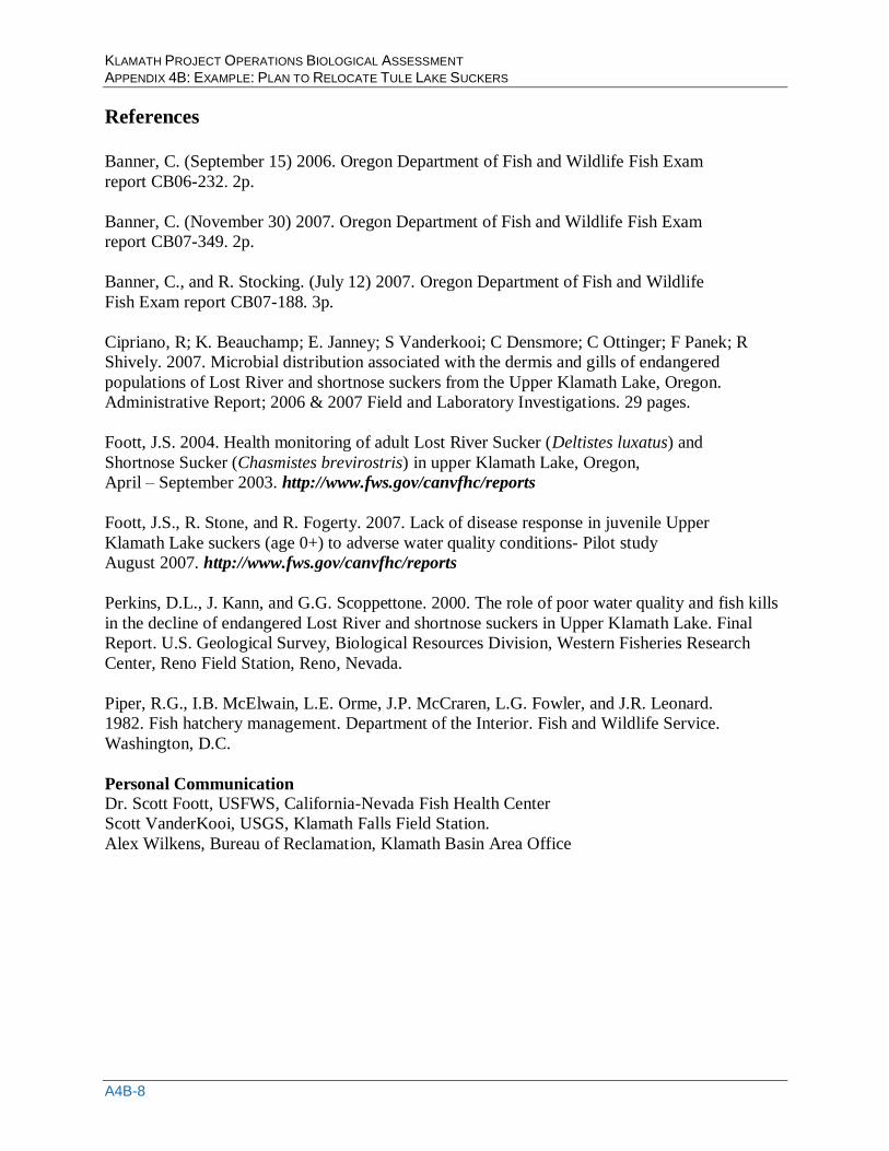
KLAMATH PROJECT OPERATIONS BIOLOGICAL ASSESSMENT APPENDIX 4B: EXAMPLE: PLAN TO RELOCATE TULE LAKE SUCKERS
A4B-8
References
Banner, C. (September 15) 2006. Oregon Department of Fish and Wildlife Fish Exam
report CB06-232. 2p.
Banner, C. (November 30) 2007. Oregon Department of Fish and Wildlife Fish Exam
report CB07-349. 2p.
Banner, C., and R. Stocking. (July 12) 2007. Oregon Department of Fish and Wildlife
Fish Exam report CB07-188. 3p.
Cipriano, R; K. Beauchamp; E. Janney; S Vanderkooi; C Densmore; C Ottinger; F Panek; R
Shively. 2007. Microbial distribution associated with the dermis and gills of endangered
populations of Lost River and shortnose suckers from the Upper Klamath Lake, Oregon.
Administrative Report; 2006 & 2007 Field and Laboratory Investigations. 29 pages.
Foott, J.S. 2004. Health monitoring of adult Lost River Sucker (Deltistes luxatus) and
Shortnose Sucker (Chasmistes brevirostris) in upper Klamath Lake, Oregon,
April – September 2003. http://www.fws.gov/canvfhc/reports
Foott, J.S., R. Stone, and R. Fogerty. 2007. Lack of disease response in juvenile Upper
Klamath Lake suckers (age 0+) to adverse water quality conditions- Pilot study
August 2007. http://www.fws.gov/canvfhc/reports
Perkins, D.L., J. Kann, and G.G. Scoppettone. 2000. The role of poor water quality and fish kills
in the decline of endangered Lost River and shortnose suckers in Upper Klamath Lake. Final
Report. U.S. Geological Survey, Biological Resources Division, Western Fisheries Research
Center, Reno Field Station, Reno, Nevada.
Piper, R.G., I.B. McElwain, L.E. Orme, J.P. McCraren, L.G. Fowler, and J.R. Leonard.
1982. Fish hatchery management. Department of the Interior. Fish and Wildlife Service.
Washington, D.C.
Personal Communication
Dr. Scott Foott, USFWS, California-Nevada Fish Health Center
Scott VanderKooi, USGS, Klamath Falls Field Station.
Alex Wilkens, Bureau of Reclamation, Klamath Basin Area Office
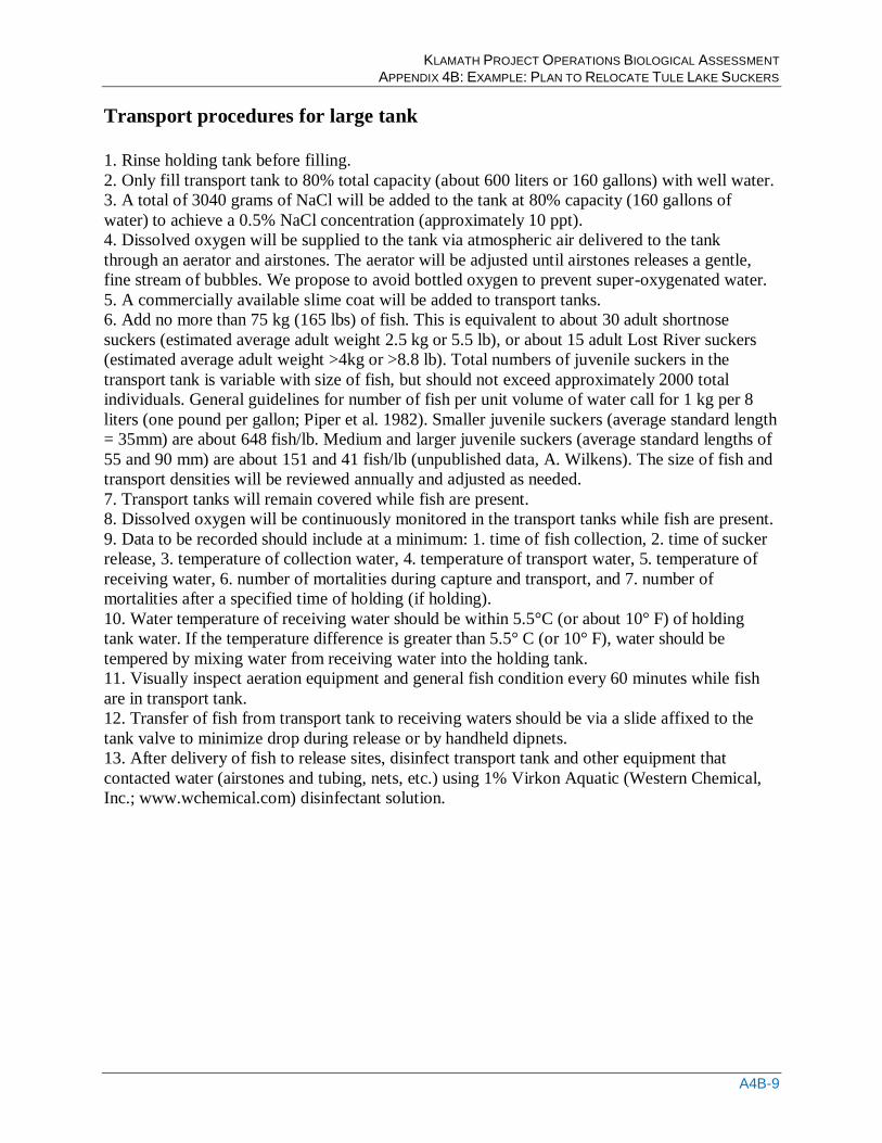
KLAMATH PROJECT OPERATIONS BIOLOGICAL ASSESSMENT APPENDIX 4B: EXAMPLE: PLAN TO RELOCATE TULE LAKE SUCKERS
A4B-9
Transport procedures for large tank
1. Rinse holding tank before filling.
2. Only fill transport tank to 80% total capacity (about 600 liters or 160 gallons) with well water.
3. A total of 3040 grams of NaCl will be added to the tank at 80% capacity (160 gallons of
water) to achieve a 0.5% NaCl concentration (approximately 10 ppt).
4. Dissolved oxygen will be supplied to the tank via atmospheric air delivered to the tank
through an aerator and airstones. The aerator will be adjusted until airstones releases a gentle,
fine stream of bubbles. We propose to avoid bottled oxygen to prevent super-oxygenated water.
5. A commercially available slime coat will be added to transport tanks.
6. Add no more than 75 kg (165 lbs) of fish. This is equivalent to about 30 adult shortnose
suckers (estimated average adult weight 2.5 kg or 5.5 lb), or about 15 adult Lost River suckers
(estimated average adult weight >4kg or >8.8 lb). Total numbers of juvenile suckers in the
transport tank is variable with size of fish, but should not exceed approximately 2000 total
individuals. General guidelines for number of fish per unit volume of water call for 1 kg per 8
liters (one pound per gallon; Piper et al. 1982). Smaller juvenile suckers (average standard length
= 35mm) are about 648 fish/lb. Medium and larger juvenile suckers (average standard lengths of
55 and 90 mm) are about 151 and 41 fish/lb (unpublished data, A. Wilkens). The size of fish and
transport densities will be reviewed annually and adjusted as needed.
7. Transport tanks will remain covered while fish are present.
8. Dissolved oxygen will be continuously monitored in the transport tanks while fish are present.
9. Data to be recorded should include at a minimum: 1. time of fish collection, 2. time of sucker
release, 3. temperature of collection water, 4. temperature of transport water, 5. temperature of
receiving water, 6. number of mortalities during capture and transport, and 7. number of
mortalities after a specified time of holding (if holding).
10. Water temperature of receiving water should be within 5.5°C (or about 10° F) of holding
tank water. If the temperature difference is greater than 5.5° C (or 10° F), water should be
tempered by mixing water from receiving water into the holding tank.
11. Visually inspect aeration equipment and general fish condition every 60 minutes while fish
are in transport tank.
12. Transfer of fish from transport tank to receiving waters should be via a slide affixed to the
tank valve to minimize drop during release or by handheld dipnets.
13. After delivery of fish to release sites, disinfect transport tank and other equipment that
contacted water (airstones and tubing, nets, etc.) using 1% Virkon Aquatic (Western Chemical,
Inc.; www.wchemical.com) disinfectant solution.
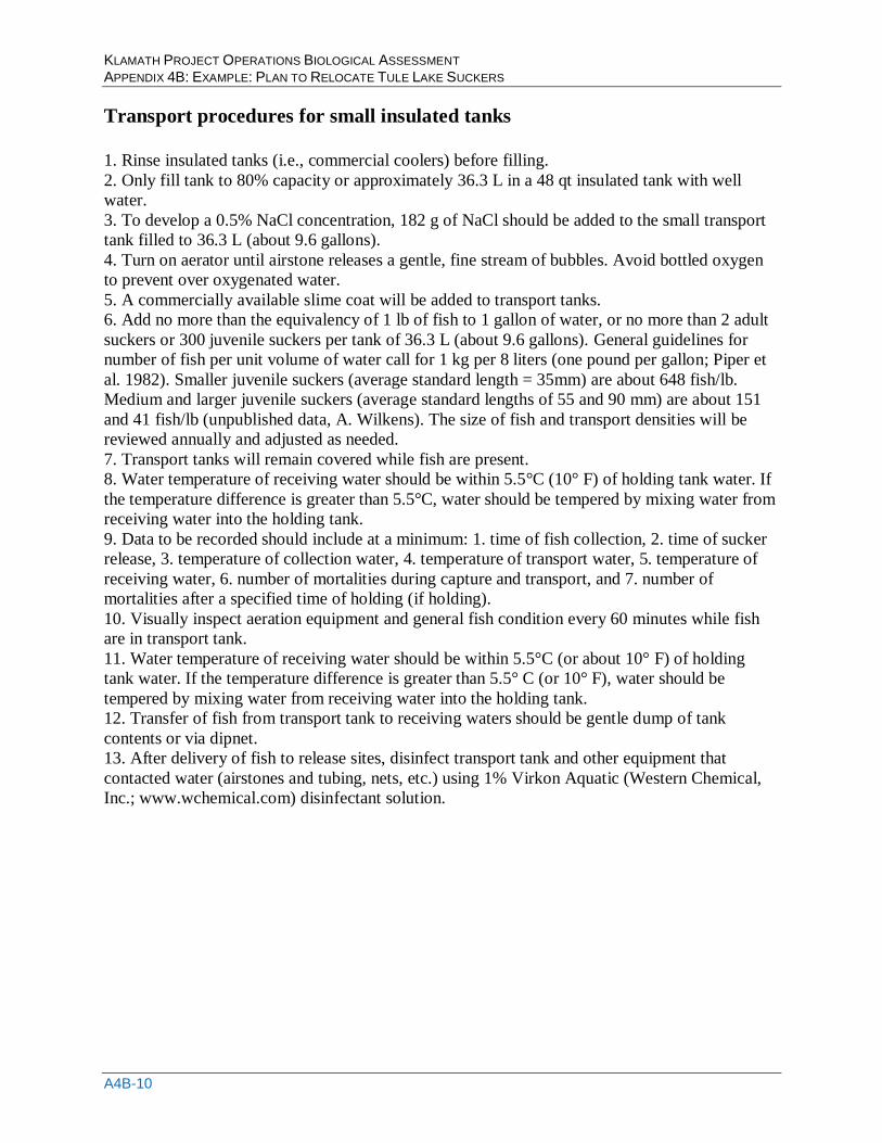
KLAMATH PROJECT OPERATIONS BIOLOGICAL ASSESSMENT APPENDIX 4B: EXAMPLE: PLAN TO RELOCATE TULE LAKE SUCKERS
A4B-10
Transport procedures for small insulated tanks
1. Rinse insulated tanks (i.e., commercial coolers) before filling.
2. Only fill tank to 80% capacity or approximately 36.3 L in a 48 qt insulated tank with well
water.
3. To develop a 0.5% NaCl concentration, 182 g of NaCl should be added to the small transport
tank filled to 36.3 L (about 9.6 gallons).
4. Turn on aerator until airstone releases a gentle, fine stream of bubbles. Avoid bottled oxygen
to prevent over oxygenated water.
5. A commercially available slime coat will be added to transport tanks.
6. Add no more than the equivalency of 1 lb of fish to 1 gallon of water, or no more than 2 adult
suckers or 300 juvenile suckers per tank of 36.3 L (about 9.6 gallons). General guidelines for
number of fish per unit volume of water call for 1 kg per 8 liters (one pound per gallon; Piper et
al. 1982). Smaller juvenile suckers (average standard length = 35mm) are about 648 fish/lb.
Medium and larger juvenile suckers (average standard lengths of 55 and 90 mm) are about 151
and 41 fish/lb (unpublished data, A. Wilkens). The size of fish and transport densities will be
reviewed annually and adjusted as needed.
7. Transport tanks will remain covered while fish are present.
8. Water temperature of receiving water should be within 5.5°C (10° F) of holding tank water. If
the temperature difference is greater than 5.5°C, water should be tempered by mixing water from
receiving water into the holding tank.
9. Data to be recorded should include at a minimum: 1. time of fish collection, 2. time of sucker
release, 3. temperature of collection water, 4. temperature of transport water, 5. temperature of
receiving water, 6. number of mortalities during capture and transport, and 7. number of
mortalities after a specified time of holding (if holding).
10. Visually inspect aeration equipment and general fish condition every 60 minutes while fish
are in transport tank.
11. Water temperature of receiving water should be within 5.5°C (or about 10° F) of holding
tank water. If the temperature difference is greater than 5.5° C (or 10° F), water should be
tempered by mixing water from receiving water into the holding tank.
12. Transfer of fish from transport tank to receiving waters should be gentle dump of tank
contents or via dipnet.
13. After delivery of fish to release sites, disinfect transport tank and other equipment that
contacted water (airstones and tubing, nets, etc.) using 1% Virkon Aquatic (Western Chemical,
Inc.; www.wchemical.com) disinfectant solution.

KLAMATH PROJECT OPERATIONS BIOLOGICAL ASSESSMENT APPENDIX 6A: CLEAR LAKE RESERVOIR END OF MONTH SURFACE ELEVATIONS
Appendix 6A: Clear Lake Reservoir End of Month Surface Elevations

KLAMATH PROJECT OPERATIONS BIOLOGICAL ASSESSMENT APPENDIX 6A: CLEAR LAKE RESERVOIR END OF MONTH SURFACE ELEVATIONS
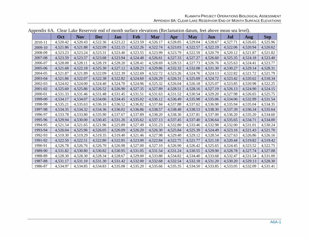
KLAMATH PROJECT OPERATIONS BIOLOGICAL ASSESSMENT APPENDIX 6A: CLEAR LAKE RESERVOIR END OF MONTH SURFACE ELEVATIONS
A6A-1
Appendix 6A. Clear Lake Reservoir end of month surface elevations (Reclamation datum, feet above mean sea level).
Oct Nov Dec Jan Feb Mar Apr May Jun Jul Aug Sep 2010-11 4,520.42 4,520.43 4,522.36 4,523.22 4,523.59 4,526.17 4,528.85 4,529.04 4,528.67 4,527.71 4,526.65 4,525.96
2009-10 4,521.86 4,521.88 4,522.09 4,522.15 4,522.26 4,522.74 4,523.03 4,522.57 4,522.19 4,522.06 4,520.94 4,520.62
2008-09 4,523.23 4,523.24 4,523.31 4,523.40 4,523.55 4,523.99 4,523.79 4,522.59 4,520.79 4,520.12 4,521.87 4,521.82
2007-08 4,523.59 4,523.57 4,523.68 4,523.94 4,524.48 4,526.61 4,527.33 4,527.27 4,526.60 4,525.35 4,524.18 4,523.40
2006-07 4,528.08 4,528.11 4,528.19 4,528.20 4,528.41 4,528.69 4,528.53 4,527.73 4,526.76 4,525.63 4,524.41 4,523.77
2005-06 4,521.68 4,522.18 4,525.30 4,527.12 4,528.23 4,529.86 4,532.32 4,532.08 4,531.30 4,530.27 4,529.14 4,528.31
2004-05 4,521.87 4,521.89 4,522.09 4,522.39 4,522.69 4,522.72 4,523.26 4,524.76 4,524.13 4,522.82 4,521.72 4,521.79
2003-04 4,521.86 4,522.07 4,522.38 4,522.82 4,524.60 4,526.29 4,526.31 4,525.69 4,524.72 4,523.42 4,520.62 4,518.34
2002-03 4,524.02 4,524.00 4,524.40 4,524.70 4,524.96 4,525.32 4,526.04 4,526.18 4,525.07 4,523.85 4,520.98 4,522.25
2001-02 4,525.60 4,525.86 4,526.52 4,526.90 4,527.35 4,527.89 4,528.51 4,528.16 4,527.19 4,526.13 4,524.90 4,524.15
2000-01 4,531.33 4,531.46 4,531.48 4,531.45 4,531.51 4,531.63 4,531.52 4,530.54 4,529.20 4,527.98 4,526.65 4,525.75
1999-00 4,534.17 4,534.07 4,534.06 4,534.45 4,535.02 4,536.12 4,536.49 4,535.98 4,535.06 4,534.06 4,532.99 4,531.54
1998-99 4,535.21 4,535.63 4,536.16 4,536.52 4,536.82 4,537.84 4,537.88 4,537.62 4,536.90 4,535.94 4,535.04 4,534.35
1997-98 4,534.35 4,534.32 4,534.36 4,536.02 4,536.86 4,538.57 4,538.48 4,538.53 4,538.30 4,537.39 4,536.34 4,535.64
1996-97 4,533.78 4,533.80 4,535.90 4,537.67 4,537.89 4,538.20 4,538.30 4,537.81 4,537.00 4,536.20 4,535.20 4,534.60
1995-96 4,529.94 4,530.00 4,530.45 4,531.26 4,535.62 4,537.13 4,537.45 4,537.40 4,536.64 4,535.65 4,534.71 4,534.00
1994-95 4,521.54 4,521.65 4,521.96 4,525.89 4,527.49 4,531.23 4,532.80 4,533.46 4,532.98 4,532.00 4,531.01 4,530.24
1993-94 4,526.04 4,525.96 4,526.05 4,526.09 4,526.20 4,526.30 4,525.84 4,525.39 4,524.49 4,523.16 4,521.43 4,521.70
1992-93 4,519.30 4,519.29 4,519.35 4,519.40 4,521.46 4,527.98 4,529.40 4,529.12 4,528.54 4,527.63 4,526.86 4,526.16
1991-92 4,522.50 4,522.51 4,522.80 4,522.85 4,523.00 4,522.84 4,522.75 4,521.77 4,521.18 4,520.44 4,519.82 4,519.42
1990-91 4,526.78 4,526.76 4,526.70 4,526.98 4,527.00 4,527.10 4,526.90 4,526.42 4,525.65 4,524.45 4,523.52 4,522.75
1989-90 4,531.82 4,530.80 4,530.82 4,530.95 4,531.05 4,531.54 4,531.24 4,530.55 4,529.90 4,528.78 4,527.74 4,527.08
1988-89 4,528.30 4,528.30 4,528.34 4,528.67 4,529.00 4,533.88 4,534.82 4,534.40 4,533.68 4,532.47 4,531.54 4,531.00
1987-88 4,531.17 4,531.10 4,531.30 4,531.42 4,532.00 4,532.68 4,532.54 4,532.18 4,531.20 4,530.20 4,529.13 4,528.30
1986-87 4,534.97 4,534.85 4,534.83 4,535.08 4,535.20 4,535.66 4,535.35 4,534.50 4,533.85 4,533.05 4,532.09 4,531.41
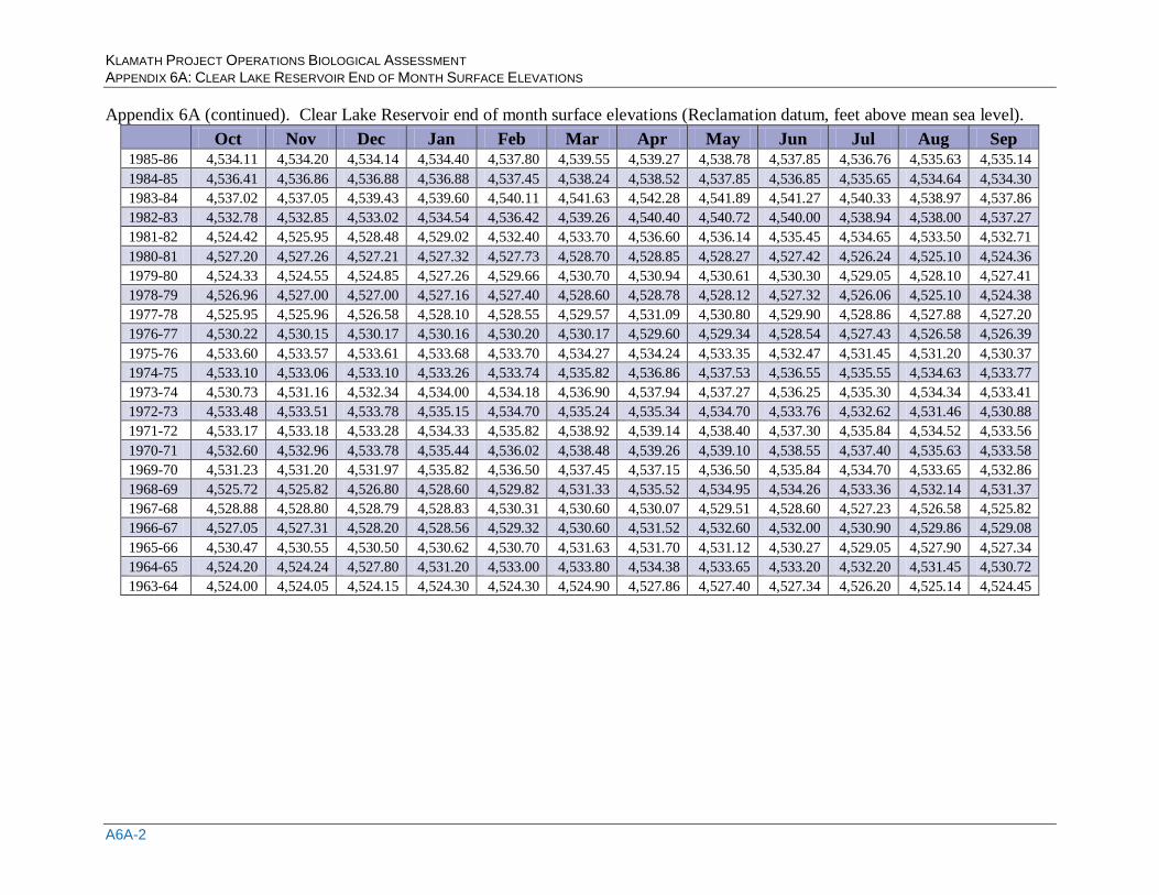
KLAMATH PROJECT OPERATIONS BIOLOGICAL ASSESSMENT APPENDIX 6A: CLEAR LAKE RESERVOIR END OF MONTH SURFACE ELEVATIONS
A6A-2
Appendix 6A (continued). Clear Lake Reservoir end of month surface elevations (Reclamation datum, feet above mean sea level).
Oct Nov Dec Jan Feb Mar Apr May Jun Jul Aug Sep 1985-86 4,534.11 4,534.20 4,534.14 4,534.40 4,537.80 4,539.55 4,539.27 4,538.78 4,537.85 4,536.76 4,535.63 4,535.14
1984-85 4,536.41 4,536.86 4,536.88 4,536.88 4,537.45 4,538.24 4,538.52 4,537.85 4,536.85 4,535.65 4,534.64 4,534.30
1983-84 4,537.02 4,537.05 4,539.43 4,539.60 4,540.11 4,541.63 4,542.28 4,541.89 4,541.27 4,540.33 4,538.97 4,537.86
1982-83 4,532.78 4,532.85 4,533.02 4,534.54 4,536.42 4,539.26 4,540.40 4,540.72 4,540.00 4,538.94 4,538.00 4,537.27
1981-82 4,524.42 4,525.95 4,528.48 4,529.02 4,532.40 4,533.70 4,536.60 4,536.14 4,535.45 4,534.65 4,533.50 4,532.71
1980-81 4,527.20 4,527.26 4,527.21 4,527.32 4,527.73 4,528.70 4,528.85 4,528.27 4,527.42 4,526.24 4,525.10 4,524.36
1979-80 4,524.33 4,524.55 4,524.85 4,527.26 4,529.66 4,530.70 4,530.94 4,530.61 4,530.30 4,529.05 4,528.10 4,527.41
1978-79 4,526.96 4,527.00 4,527.00 4,527.16 4,527.40 4,528.60 4,528.78 4,528.12 4,527.32 4,526.06 4,525.10 4,524.38
1977-78 4,525.95 4,525.96 4,526.58 4,528.10 4,528.55 4,529.57 4,531.09 4,530.80 4,529.90 4,528.86 4,527.88 4,527.20
1976-77 4,530.22 4,530.15 4,530.17 4,530.16 4,530.20 4,530.17 4,529.60 4,529.34 4,528.54 4,527.43 4,526.58 4,526.39
1975-76 4,533.60 4,533.57 4,533.61 4,533.68 4,533.70 4,534.27 4,534.24 4,533.35 4,532.47 4,531.45 4,531.20 4,530.37
1974-75 4,533.10 4,533.06 4,533.10 4,533.26 4,533.74 4,535.82 4,536.86 4,537.53 4,536.55 4,535.55 4,534.63 4,533.77
1973-74 4,530.73 4,531.16 4,532.34 4,534.00 4,534.18 4,536.90 4,537.94 4,537.27 4,536.25 4,535.30 4,534.34 4,533.41
1972-73 4,533.48 4,533.51 4,533.78 4,535.15 4,534.70 4,535.24 4,535.34 4,534.70 4,533.76 4,532.62 4,531.46 4,530.88
1971-72 4,533.17 4,533.18 4,533.28 4,534.33 4,535.82 4,538.92 4,539.14 4,538.40 4,537.30 4,535.84 4,534.52 4,533.56
1970-71 4,532.60 4,532.96 4,533.78 4,535.44 4,536.02 4,538.48 4,539.26 4,539.10 4,538.55 4,537.40 4,535.63 4,533.58
1969-70 4,531.23 4,531.20 4,531.97 4,535.82 4,536.50 4,537.45 4,537.15 4,536.50 4,535.84 4,534.70 4,533.65 4,532.86
1968-69 4,525.72 4,525.82 4,526.80 4,528.60 4,529.82 4,531.33 4,535.52 4,534.95 4,534.26 4,533.36 4,532.14 4,531.37
1967-68 4,528.88 4,528.80 4,528.79 4,528.83 4,530.31 4,530.60 4,530.07 4,529.51 4,528.60 4,527.23 4,526.58 4,525.82
1966-67 4,527.05 4,527.31 4,528.20 4,528.56 4,529.32 4,530.60 4,531.52 4,532.60 4,532.00 4,530.90 4,529.86 4,529.08
1965-66 4,530.47 4,530.55 4,530.50 4,530.62 4,530.70 4,531.63 4,531.70 4,531.12 4,530.27 4,529.05 4,527.90 4,527.34
1964-65 4,524.20 4,524.24 4,527.80 4,531.20 4,533.00 4,533.80 4,534.38 4,533.65 4,533.20 4,532.20 4,531.45 4,530.72
1963-64 4,524.00 4,524.05 4,524.15 4,524.30 4,524.30 4,524.90 4,527.86 4,527.40 4,527.34 4,526.20 4,525.14 4,524.45
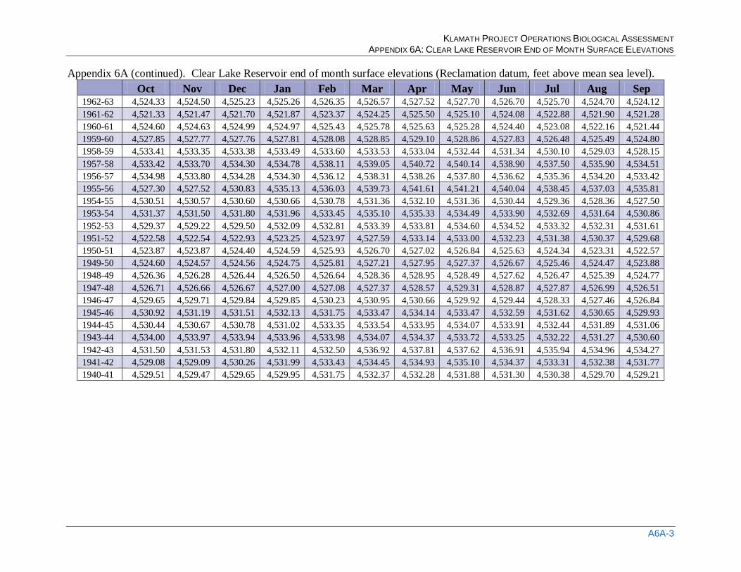
KLAMATH PROJECT OPERATIONS BIOLOGICAL ASSESSMENT APPENDIX 6A: CLEAR LAKE RESERVOIR END OF MONTH SURFACE ELEVATIONS
A6A-3
Appendix 6A (continued). Clear Lake Reservoir end of month surface elevations (Reclamation datum, feet above mean sea level).
Oct Nov Dec Jan Feb Mar Apr May Jun Jul Aug Sep 1962-63 4,524.33 4,524.50 4,525.23 4,525.26 4,526.35 4,526.57 4,527.52 4,527.70 4,526.70 4,525.70 4,524.70 4,524.12
1961-62 4,521.33 4,521.47 4,521.70 4,521.87 4,523.37 4,524.25 4,525.50 4,525.10 4,524.08 4,522.88 4,521.90 4,521.28
1960-61 4,524.60 4,524.63 4,524.99 4,524.97 4,525.43 4,525.78 4,525.63 4,525.28 4,524.40 4,523.08 4,522.16 4,521.44
1959-60 4,527.85 4,527.77 4,527.76 4,527.81 4,528.08 4,528.85 4,529.10 4,528.86 4,527.83 4,526.48 4,525.49 4,524.80
1958-59 4,533.41 4,533.35 4,533.38 4,533.49 4,533.60 4,533.53 4,533.04 4,532.44 4,531.34 4,530.10 4,529.03 4,528.15
1957-58 4,533.42 4,533.70 4,534.30 4,534.78 4,538.11 4,539.05 4,540.72 4,540.14 4,538.90 4,537.50 4,535.90 4,534.51
1956-57 4,534.98 4,533.80 4,534.28 4,534.30 4,536.12 4,538.31 4,538.26 4,537.80 4,536.62 4,535.36 4,534.20 4,533.42
1955-56 4,527.30 4,527.52 4,530.83 4,535.13 4,536.03 4,539.73 4,541.61 4,541.21 4,540.04 4,538.45 4,537.03 4,535.81
1954-55 4,530.51 4,530.57 4,530.60 4,530.66 4,530.78 4,531.36 4,532.10 4,531.36 4,530.44 4,529.36 4,528.36 4,527.50
1953-54 4,531.37 4,531.50 4,531.80 4,531.96 4,533.45 4,535.10 4,535.33 4,534.49 4,533.90 4,532.69 4,531.64 4,530.86
1952-53 4,529.37 4,529.22 4,529.50 4,532.09 4,532.81 4,533.39 4,533.81 4,534.60 4,534.52 4,533.32 4,532.31 4,531.61
1951-52 4,522.58 4,522.54 4,522.93 4,523.25 4,523.97 4,527.59 4,533.14 4,533.00 4,532.23 4,531.38 4,530.37 4,529.68
1950-51 4,523.87 4,523.87 4,524.40 4,524.59 4,525.93 4,526.70 4,527.02 4,526.84 4,525.63 4,524.34 4,523.31 4,522.57
1949-50 4,524.60 4,524.57 4,524.56 4,524.75 4,525.81 4,527.21 4,527.95 4,527.37 4,526.67 4,525.46 4,524.47 4,523.88
1948-49 4,526.36 4,526.28 4,526.44 4,526.50 4,526.64 4,528.36 4,528.95 4,528.49 4,527.62 4,526.47 4,525.39 4,524.77
1947-48 4,526.71 4,526.66 4,526.67 4,527.00 4,527.08 4,527.37 4,528.57 4,529.31 4,528.87 4,527.87 4,526.99 4,526.51
1946-47 4,529.65 4,529.71 4,529.84 4,529.85 4,530.23 4,530.95 4,530.66 4,529.92 4,529.44 4,528.33 4,527.46 4,526.84
1945-46 4,530.92 4,531.19 4,531.51 4,532.13 4,531.75 4,533.47 4,534.14 4,533.47 4,532.59 4,531.62 4,530.65 4,529.93
1944-45 4,530.44 4,530.67 4,530.78 4,531.02 4,533.35 4,533.54 4,533.95 4,534.07 4,533.91 4,532.44 4,531.89 4,531.06
1943-44 4,534.00 4,533.97 4,533.94 4,533.96 4,533.98 4,534.07 4,534.37 4,533.72 4,533.25 4,532.22 4,531.27 4,530.60
1942-43 4,531.50 4,531.53 4,531.80 4,532.11 4,532.50 4,536.92 4,537.81 4,537.62 4,536.91 4,535.94 4,534.96 4,534.27
1941-42 4,529.08 4,529.09 4,530.26 4,531.99 4,533.43 4,534.45 4,534.93 4,535.10 4,534.37 4,533.31 4,532.38 4,531.77
1940-41 4,529.51 4,529.47 4,529.65 4,529.95 4,531.75 4,532.37 4,532.28 4,531.88 4,531.30 4,530.38 4,529.70 4,529.21
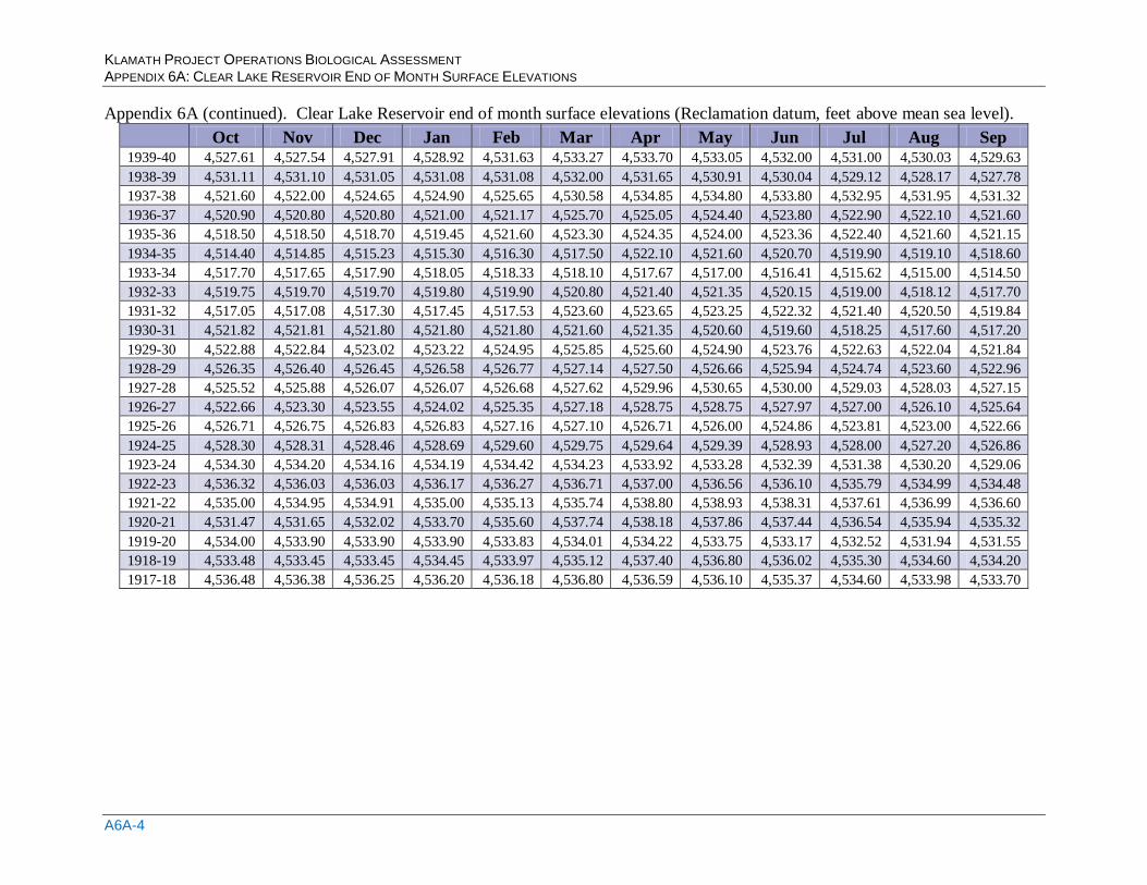
KLAMATH PROJECT OPERATIONS BIOLOGICAL ASSESSMENT APPENDIX 6A: CLEAR LAKE RESERVOIR END OF MONTH SURFACE ELEVATIONS
A6A-4
Appendix 6A (continued). Clear Lake Reservoir end of month surface elevations (Reclamation datum, feet above mean sea level).
Oct Nov Dec Jan Feb Mar Apr May Jun Jul Aug Sep 1939-40 4,527.61 4,527.54 4,527.91 4,528.92 4,531.63 4,533.27 4,533.70 4,533.05 4,532.00 4,531.00 4,530.03 4,529.63
1938-39 4,531.11 4,531.10 4,531.05 4,531.08 4,531.08 4,532.00 4,531.65 4,530.91 4,530.04 4,529.12 4,528.17 4,527.78
1937-38 4,521.60 4,522.00 4,524.65 4,524.90 4,525.65 4,530.58 4,534.85 4,534.80 4,533.80 4,532.95 4,531.95 4,531.32
1936-37 4,520.90 4,520.80 4,520.80 4,521.00 4,521.17 4,525.70 4,525.05 4,524.40 4,523.80 4,522.90 4,522.10 4,521.60
1935-36 4,518.50 4,518.50 4,518.70 4,519.45 4,521.60 4,523.30 4,524.35 4,524.00 4,523.36 4,522.40 4,521.60 4,521.15
1934-35 4,514.40 4,514.85 4,515.23 4,515.30 4,516.30 4,517.50 4,522.10 4,521.60 4,520.70 4,519.90 4,519.10 4,518.60
1933-34 4,517.70 4,517.65 4,517.90 4,518.05 4,518.33 4,518.10 4,517.67 4,517.00 4,516.41 4,515.62 4,515.00 4,514.50
1932-33 4,519.75 4,519.70 4,519.70 4,519.80 4,519.90 4,520.80 4,521.40 4,521.35 4,520.15 4,519.00 4,518.12 4,517.70
1931-32 4,517.05 4,517.08 4,517.30 4,517.45 4,517.53 4,523.60 4,523.65 4,523.25 4,522.32 4,521.40 4,520.50 4,519.84
1930-31 4,521.82 4,521.81 4,521.80 4,521.80 4,521.80 4,521.60 4,521.35 4,520.60 4,519.60 4,518.25 4,517.60 4,517.20
1929-30 4,522.88 4,522.84 4,523.02 4,523.22 4,524.95 4,525.85 4,525.60 4,524.90 4,523.76 4,522.63 4,522.04 4,521.84
1928-29 4,526.35 4,526.40 4,526.45 4,526.58 4,526.77 4,527.14 4,527.50 4,526.66 4,525.94 4,524.74 4,523.60 4,522.96
1927-28 4,525.52 4,525.88 4,526.07 4,526.07 4,526.68 4,527.62 4,529.96 4,530.65 4,530.00 4,529.03 4,528.03 4,527.15
1926-27 4,522.66 4,523.30 4,523.55 4,524.02 4,525.35 4,527.18 4,528.75 4,528.75 4,527.97 4,527.00 4,526.10 4,525.64
1925-26 4,526.71 4,526.75 4,526.83 4,526.83 4,527.16 4,527.10 4,526.71 4,526.00 4,524.86 4,523.81 4,523.00 4,522.66
1924-25 4,528.30 4,528.31 4,528.46 4,528.69 4,529.60 4,529.75 4,529.64 4,529.39 4,528.93 4,528.00 4,527.20 4,526.86
1923-24 4,534.30 4,534.20 4,534.16 4,534.19 4,534.42 4,534.23 4,533.92 4,533.28 4,532.39 4,531.38 4,530.20 4,529.06
1922-23 4,536.32 4,536.03 4,536.03 4,536.17 4,536.27 4,536.71 4,537.00 4,536.56 4,536.10 4,535.79 4,534.99 4,534.48
1921-22 4,535.00 4,534.95 4,534.91 4,535.00 4,535.13 4,535.74 4,538.80 4,538.93 4,538.31 4,537.61 4,536.99 4,536.60
1920-21 4,531.47 4,531.65 4,532.02 4,533.70 4,535.60 4,537.74 4,538.18 4,537.86 4,537.44 4,536.54 4,535.94 4,535.32
1919-20 4,534.00 4,533.90 4,533.90 4,533.90 4,533.83 4,534.01 4,534.22 4,533.75 4,533.17 4,532.52 4,531.94 4,531.55
1918-19 4,533.48 4,533.45 4,533.45 4,534.45 4,533.97 4,535.12 4,537.40 4,536.80 4,536.02 4,535.30 4,534.60 4,534.20
1917-18 4,536.48 4,536.38 4,536.25 4,536.20 4,536.18 4,536.80 4,536.59 4,536.10 4,535.37 4,534.60 4,533.98 4,533.70
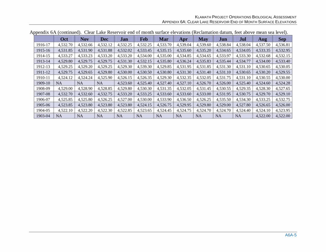
KLAMATH PROJECT OPERATIONS BIOLOGICAL ASSESSMENT APPENDIX 6A: CLEAR LAKE RESERVOIR END OF MONTH SURFACE ELEVATIONS
A6A-5
Appendix 6A (continued). Clear Lake Reservoir end of month surface elevations (Reclamation datum, feet above mean sea level).
Oct Nov Dec Jan Feb Mar Apr May Jun Jul Aug Sep 1916-17 4,532.70 4,532.66 4,532.12 4,532.25 4,532.25 4,533.70 4,539.04 4,539.60 4,538.84 4,538.04 4,537.50 4,536.81
1915-16 4,531.85 4,531.90 4,531.88 4,532.02 4,533.45 4,535.15 4,535.60 4,535.20 4,534.65 4,534.05 4,533.35 4,532.95
1914-15 4,533.27 4,533.23 4,533.20 4,533.20 4,534.00 4,535.00 4,534.85 4,534.65 4,533.97 4,533.30 4,532.68 4,532.15
1913-14 4,529.80 4,529.75 4,529.75 4,531.30 4,532.15 4,535.80 4,536.24 4,535.83 4,535.44 4,534.77 4,534.00 4,533.40
1912-13 4,529.25 4,529.20 4,529.25 4,529.30 4,539.30 4,529.85 4,531.95 4,531.85 4,531.30 4,531.10 4,530.65 4,530.05
1911-12 4,529.75 4,529.65 4,529.80 4,530.00 4,530.50 4,530.80 4,531.30 4,531.40 4,531.10 4,530.65 4,530.20 4,529.55
1910-11 4,524.12 4,524.24 4,525.90 4,526.15 4,526.35 4,529.30 4,532.35 4,532.05 4,531.75 4,531.10 4,530.55 4,530.00
1909-10 NA NA NA 4,523.60 4,525.40 4,527.40 4,527.10 4,526.70 4,526.00 4,525.40 4,524.60 4,524.28
1908-09 4,529.00 4,528.90 4,528.85 4,529.80 4,530.30 4,531.35 4,532.05 4,531.45 4,530.55 4,529.35 4,528.30 4,527.65
1907-08 4,532.70 4,532.60 4,532.75 4,533.20 4,533.25 4,533.60 4,533.60 4,533.00 4,531.95 4,530.75 4,529.70 4,529.10
1906-07 4,525.85 4,525.80 4,526.25 4,527.00 4,530.00 4,533.90 4,536.50 4,526.25 4,535.50 4,534.30 4,533.25 4,532.75
1905-06 4,523.85 4,523.80 4,523.80 4,523.80 4,524.15 4,526.75 4,529.95 4,529.80 4,529.00 4,527.80 4,526.65 4,526.00
1904-05 4,522.10 4,522.20 4,522.30 4,522.85 4,523.65 4,524.45 4,524.75 4,524.70 4,524.70 4,524.40 4,524.10 4,523.95
1903-04 NA NA NA NA NA NA NA NA NA NA 4,522.00 4,522.00

KLAMATH PROJECT OPERATIONS BIOLOGICAL ASSESSMENT APPENDIX 6A: CLEAR LAKE RESERVOIR END OF MONTH SURFACE ELEVATIONS
A6A-6
End of Appendix 6A

KLAMATH PROJECT OPERATIONS BIOLOGICAL ASSESSMENT APPENDIX 6B: GERBER RESERVOIR OBSERVED END OF MONTH SURFACE ELEVATIONS
Appendix 6B: Gerber Reservoir Observed End of Month Surface Elevations

KLAMATH PROJECT OPERATIONS BIOLOGICAL ASSESSMENT APPENDIX 6B: GERBER RESERVOIR OBSERVED END OF MONTH SURFACE ELEVATIONS
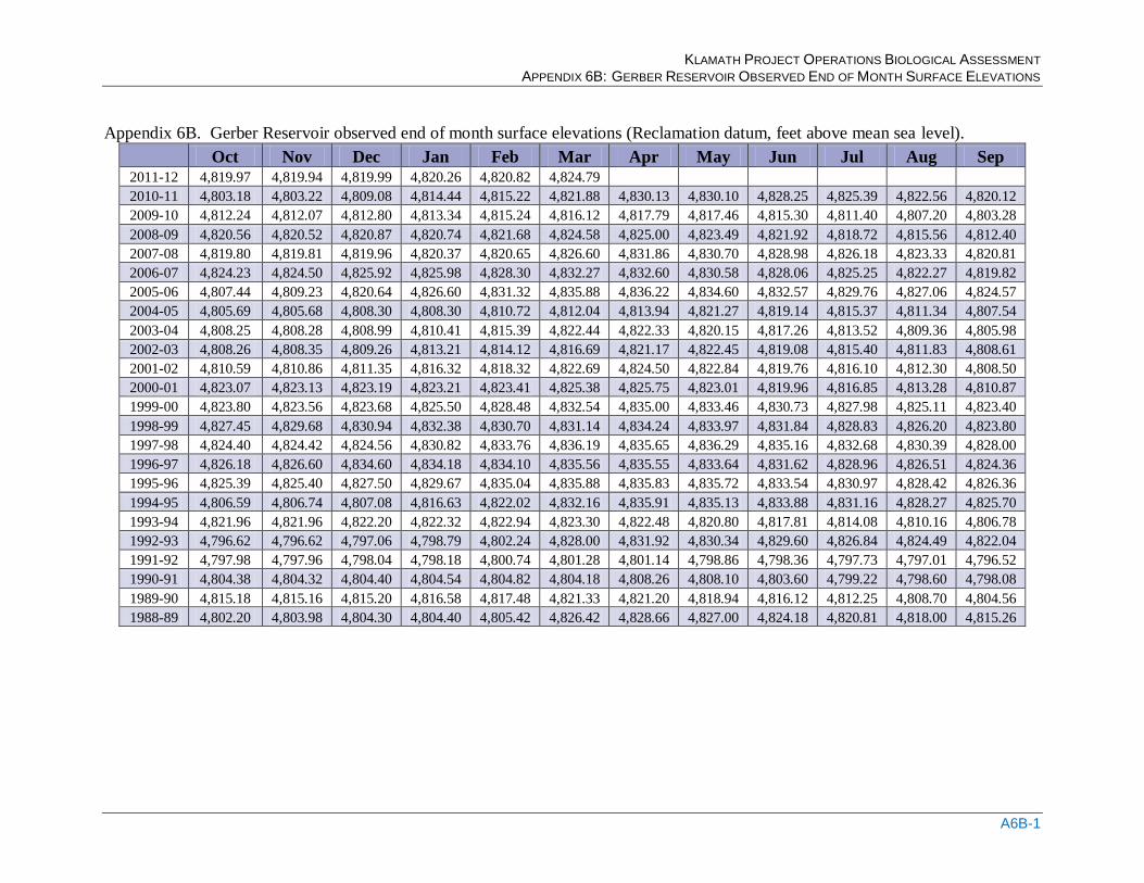
KLAMATH PROJECT OPERATIONS BIOLOGICAL ASSESSMENT APPENDIX 6B: GERBER RESERVOIR OBSERVED END OF MONTH SURFACE ELEVATIONS
A6B-1
Appendix 6B. Gerber Reservoir observed end of month surface elevations (Reclamation datum, feet above mean sea level).
Oct Nov Dec Jan Feb Mar Apr May Jun Jul Aug Sep
2011-12 4,819.97 4,819.94 4,819.99 4,820.26 4,820.82 4,824.79
2010-11 4,803.18 4,803.22 4,809.08 4,814.44 4,815.22 4,821.88 4,830.13 4,830.10 4,828.25 4,825.39 4,822.56 4,820.12
2009-10 4,812.24 4,812.07 4,812.80 4,813.34 4,815.24 4,816.12 4,817.79 4,817.46 4,815.30 4,811.40 4,807.20 4,803.28
2008-09 4,820.56 4,820.52 4,820.87 4,820.74 4,821.68 4,824.58 4,825.00 4,823.49 4,821.92 4,818.72 4,815.56 4,812.40
2007-08 4,819.80 4,819.81 4,819.96 4,820.37 4,820.65 4,826.60 4,831.86 4,830.70 4,828.98 4,826.18 4,823.33 4,820.81
2006-07 4,824.23 4,824.50 4,825.92 4,825.98 4,828.30 4,832.27 4,832.60 4,830.58 4,828.06 4,825.25 4,822.27 4,819.82
2005-06 4,807.44 4,809.23 4,820.64 4,826.60 4,831.32 4,835.88 4,836.22 4,834.60 4,832.57 4,829.76 4,827.06 4,824.57
2004-05 4,805.69 4,805.68 4,808.30 4,808.30 4,810.72 4,812.04 4,813.94 4,821.27 4,819.14 4,815.37 4,811.34 4,807.54
2003-04 4,808.25 4,808.28 4,808.99 4,810.41 4,815.39 4,822.44 4,822.33 4,820.15 4,817.26 4,813.52 4,809.36 4,805.98
2002-03 4,808.26 4,808.35 4,809.26 4,813.21 4,814.12 4,816.69 4,821.17 4,822.45 4,819.08 4,815.40 4,811.83 4,808.61
2001-02 4,810.59 4,810.86 4,811.35 4,816.32 4,818.32 4,822.69 4,824.50 4,822.84 4,819.76 4,816.10 4,812.30 4,808.50
2000-01 4,823.07 4,823.13 4,823.19 4,823.21 4,823.41 4,825.38 4,825.75 4,823.01 4,819.96 4,816.85 4,813.28 4,810.87
1999-00 4,823.80 4,823.56 4,823.68 4,825.50 4,828.48 4,832.54 4,835.00 4,833.46 4,830.73 4,827.98 4,825.11 4,823.40
1998-99 4,827.45 4,829.68 4,830.94 4,832.38 4,830.70 4,831.14 4,834.24 4,833.97 4,831.84 4,828.83 4,826.20 4,823.80
1997-98 4,824.40 4,824.42 4,824.56 4,830.82 4,833.76 4,836.19 4,835.65 4,836.29 4,835.16 4,832.68 4,830.39 4,828.00
1996-97 4,826.18 4,826.60 4,834.60 4,834.18 4,834.10 4,835.56 4,835.55 4,833.64 4,831.62 4,828.96 4,826.51 4,824.36
1995-96 4,825.39 4,825.40 4,827.50 4,829.67 4,835.04 4,835.88 4,835.83 4,835.72 4,833.54 4,830.97 4,828.42 4,826.36
1994-95 4,806.59 4,806.74 4,807.08 4,816.63 4,822.02 4,832.16 4,835.91 4,835.13 4,833.88 4,831.16 4,828.27 4,825.70
1993-94 4,821.96 4,821.96 4,822.20 4,822.32 4,822.94 4,823.30 4,822.48 4,820.80 4,817.81 4,814.08 4,810.16 4,806.78
1992-93 4,796.62 4,796.62 4,797.06 4,798.79 4,802.24 4,828.00 4,831.92 4,830.34 4,829.60 4,826.84 4,824.49 4,822.04
1991-92 4,797.98 4,797.96 4,798.04 4,798.18 4,800.74 4,801.28 4,801.14 4,798.86 4,798.36 4,797.73 4,797.01 4,796.52
1990-91 4,804.38 4,804.32 4,804.40 4,804.54 4,804.82 4,804.18 4,808.26 4,808.10 4,803.60 4,799.22 4,798.60 4,798.08
1989-90 4,815.18 4,815.16 4,815.20 4,816.58 4,817.48 4,821.33 4,821.20 4,818.94 4,816.12 4,812.25 4,808.70 4,804.56
1988-89 4,802.20 4,803.98 4,804.30 4,804.40 4,805.42 4,826.42 4,828.66 4,827.00 4,824.18 4,820.81 4,818.00 4,815.26
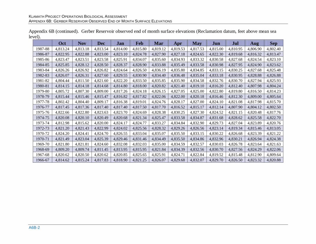
KLAMATH PROJECT OPERATIONS BIOLOGICAL ASSESSMENT APPENDIX 6B: GERBER RESERVOIR OBSERVED END OF MONTH SURFACE ELEVATIONS
A6B-2
Appendix 6B (continued). Gerber Reservoir observed end of month surface elevations (Reclamation datum, feet above mean sea
level).
Oct Nov Dec Jan Feb Mar Apr May Jun Jul Aug Sep
1987-88 4,813.24 4,813.18 4,813.54 4,814.00 4,815.80 4,819.12 4,819.53 4,817.53 4,815.00 4,810.95 4,806.90 4,802.40
1986-87 4,822.95 4,822.88 4,823.00 4,823.10 4,824.78 4,827.90 4,827.18 4,824.65 4,822.30 4,819.68 4,816.32 4,813.47
1985-86 4,823.47 4,823.51 4,823.58 4,825.91 4,834.07 4,835.60 4,834.93 4,833.32 4,830.58 4,827.68 4,824.54 4,823.10
1984-85 4,825.85 4,828.12 4,828.50 4,828.37 4,828.90 4,833.88 4,835.49 4,833.58 4,830.98 4,827.95 4,824.90 4,823.62
1983-84 4,826.26 4,826.92 4,826.82 4,824.64 4,826.50 4,836.19 4,835.80 4,834.85 4,833.15 4,830.25 4,827.68 4,825.48
1982-83 4,826.07 4,826.31 4,827.60 4,829.55 4,830.90 4,834.40 4,836.48 4,835.04 4,833.18 4,830.95 4,828.88 4,826.88
1981-82 4,804.44 4,811.50 4,821.60 4,822.20 4,833.50 4,835.85 4,835.90 4,834.58 4,832.76 4,830.70 4,827.94 4,825.93
1980-81 4,814.15 4,814.18 4,814.68 4,814.80 4,818.00 4,820.82 4,821.40 4,819.10 4,816.20 4,812.40 4,807.98 4,804.24
1979-80 4,805.72 4,807.30 4,809.00 4,817.26 4,824.18 4,826.15 4,827.05 4,825.00 4,822.80 4,819.80 4,816.50 4,814.23
1978-79 4,815.44 4,815.46 4,815.47 4,816.82 4,817.82 4,822.06 4,822.00 4,820.18 4,816.46 4,812.30 4,809.00 4,805.64
1977-78 4,802.42 4,804.40 4,809.17 4,816.38 4,819.01 4,824.76 4,828.17 4,827.00 4,824.10 4,821.08 4,817.98 4,815.70
1976-77 4,817.45 4,817.36 4,817.40 4,817.40 4,817.50 4,817.70 4,816.52 4,815.17 4,812.14 4,807.90 4,804.12 4,802.50
1975-76 4,822.66 4,822.80 4,823.63 4,823.70 4,824.69 4,828.38 4,830.25 4,827.30 4,824.52 4,821.15 4,820.48 4,817.76
1974-75 4,820.08 4,820.10 4,820.49 4,820.68 4,821.34 4,825.47 4,833.58 4,834.87 4,831.68 4,828.62 4,825.58 4,822.70
1973-74 4,812.98 4,815.62 4,820.00 4,824.17 4,824.77 4,833.27 4,834.84 4,832.90 4,829.73 4,827.04 4,823.89 4,820.76
1972-73 4,821.20 4,821.43 4,822.99 4,824.02 4,825.56 4,828.32 4,829.26 4,826.56 4,823.14 4,819.34 4,815.46 4,813.05
1970-72 4,824.20 4,824.41 4,824.70 4,826.55 4,833.04 4,835.07 4,835.50 4,833.15 4,830.22 4,826.68 4,823.39 4,821.22
1970-71 4,821.49 4,823.04 4,825.39 4,829.46 4,831.46 4,834.49 4,835.50 4,834.86 4,832.96 4,830.21 4,826.94 4,824.38
1969-70 4,821.80 4,821.81 4,824.60 4,832.08 4,832.03 4,835.00 4,834.59 4,832.57 4,830.03 4,826.78 4,823.64 4,821.63
1968-69 4,809.20 4,809.74 4,811.45 4,813.95 4,815.95 4,821.84 4,834.39 4,832.56 4,830.70 4,827.56 4,824.29 4,822.06
1967-68 4,820.62 4,820.50 4,820.62 4,820.85 4,825.65 4,825.91 4,824.71 4,822.84 4,819.52 4,815.48 4,812.90 4,809.64
1966-67 4,814.62 4,815.24 4,817.83 4,818.90 4,821.25 4,826.07 4,829.68 4,832.07 4,829.70 4,826.50 4,823.32 4,820.88
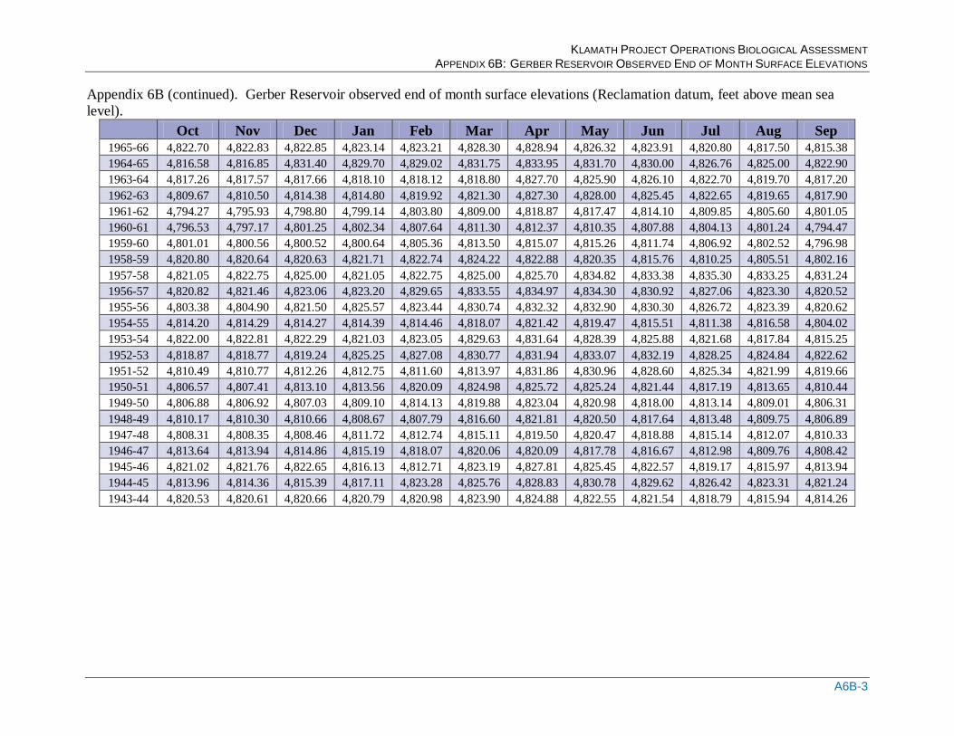
KLAMATH PROJECT OPERATIONS BIOLOGICAL ASSESSMENT APPENDIX 6B: GERBER RESERVOIR OBSERVED END OF MONTH SURFACE ELEVATIONS
A6B-3
Appendix 6B (continued). Gerber Reservoir observed end of month surface elevations (Reclamation datum, feet above mean sea
level).
Oct Nov Dec Jan Feb Mar Apr May Jun Jul Aug Sep
1965-66 4,822.70 4,822.83 4,822.85 4,823.14 4,823.21 4,828.30 4,828.94 4,826.32 4,823.91 4,820.80 4,817.50 4,815.38
1964-65 4,816.58 4,816.85 4,831.40 4,829.70 4,829.02 4,831.75 4,833.95 4,831.70 4,830.00 4,826.76 4,825.00 4,822.90
1963-64 4,817.26 4,817.57 4,817.66 4,818.10 4,818.12 4,818.80 4,827.70 4,825.90 4,826.10 4,822.70 4,819.70 4,817.20
1962-63 4,809.67 4,810.50 4,814.38 4,814.80 4,819.92 4,821.30 4,827.30 4,828.00 4,825.45 4,822.65 4,819.65 4,817.90
1961-62 4,794.27 4,795.93 4,798.80 4,799.14 4,803.80 4,809.00 4,818.87 4,817.47 4,814.10 4,809.85 4,805.60 4,801.05
1960-61 4,796.53 4,797.17 4,801.25 4,802.34 4,807.64 4,811.30 4,812.37 4,810.35 4,807.88 4,804.13 4,801.24 4,794.47
1959-60 4,801.01 4,800.56 4,800.52 4,800.64 4,805.36 4,813.50 4,815.07 4,815.26 4,811.74 4,806.92 4,802.52 4,796.98
1958-59 4,820.80 4,820.64 4,820.63 4,821.71 4,822.74 4,824.22 4,822.88 4,820.35 4,815.76 4,810.25 4,805.51 4,802.16
1957-58 4,821.05 4,822.75 4,825.00 4,821.05 4,822.75 4,825.00 4,825.70 4,834.82 4,833.38 4,835.30 4,833.25 4,831.24
1956-57 4,820.82 4,821.46 4,823.06 4,823.20 4,829.65 4,833.55 4,834.97 4,834.30 4,830.92 4,827.06 4,823.30 4,820.52
1955-56 4,803.38 4,804.90 4,821.50 4,825.57 4,823.44 4,830.74 4,832.32 4,832.90 4,830.30 4,826.72 4,823.39 4,820.62
1954-55 4,814.20 4,814.29 4,814.27 4,814.39 4,814.46 4,818.07 4,821.42 4,819.47 4,815.51 4,811.38 4,816.58 4,804.02
1953-54 4,822.00 4,822.81 4,822.29 4,821.03 4,823.05 4,829.63 4,831.64 4,828.39 4,825.88 4,821.68 4,817.84 4,815.25
1952-53 4,818.87 4,818.77 4,819.24 4,825.25 4,827.08 4,830.77 4,831.94 4,833.07 4,832.19 4,828.25 4,824.84 4,822.62
1951-52 4,810.49 4,810.77 4,812.26 4,812.75 4,811.60 4,813.97 4,831.86 4,830.96 4,828.60 4,825.34 4,821.99 4,819.66
1950-51 4,806.57 4,807.41 4,813.10 4,813.56 4,820.09 4,824.98 4,825.72 4,825.24 4,821.44 4,817.19 4,813.65 4,810.44
1949-50 4,806.88 4,806.92 4,807.03 4,809.10 4,814.13 4,819.88 4,823.04 4,820.98 4,818.00 4,813.14 4,809.01 4,806.31
1948-49 4,810.17 4,810.30 4,810.66 4,808.67 4,807.79 4,816.60 4,821.81 4,820.50 4,817.64 4,813.48 4,809.75 4,806.89
1947-48 4,808.31 4,808.35 4,808.46 4,811.72 4,812.74 4,815.11 4,819.50 4,820.47 4,818.88 4,815.14 4,812.07 4,810.33
1946-47 4,813.64 4,813.94 4,814.86 4,815.19 4,818.07 4,820.06 4,820.09 4,817.78 4,816.67 4,812.98 4,809.76 4,808.42
1945-46 4,821.02 4,821.76 4,822.65 4,816.13 4,812.71 4,823.19 4,827.81 4,825.45 4,822.57 4,819.17 4,815.97 4,813.94
1944-45 4,813.96 4,814.36 4,815.39 4,817.11 4,823.28 4,825.76 4,828.83 4,830.78 4,829.62 4,826.42 4,823.31 4,821.24
1943-44 4,820.53 4,820.61 4,820.66 4,820.79 4,820.98 4,823.90 4,824.88 4,822.55 4,821.54 4,818.79 4,815.94 4,814.26
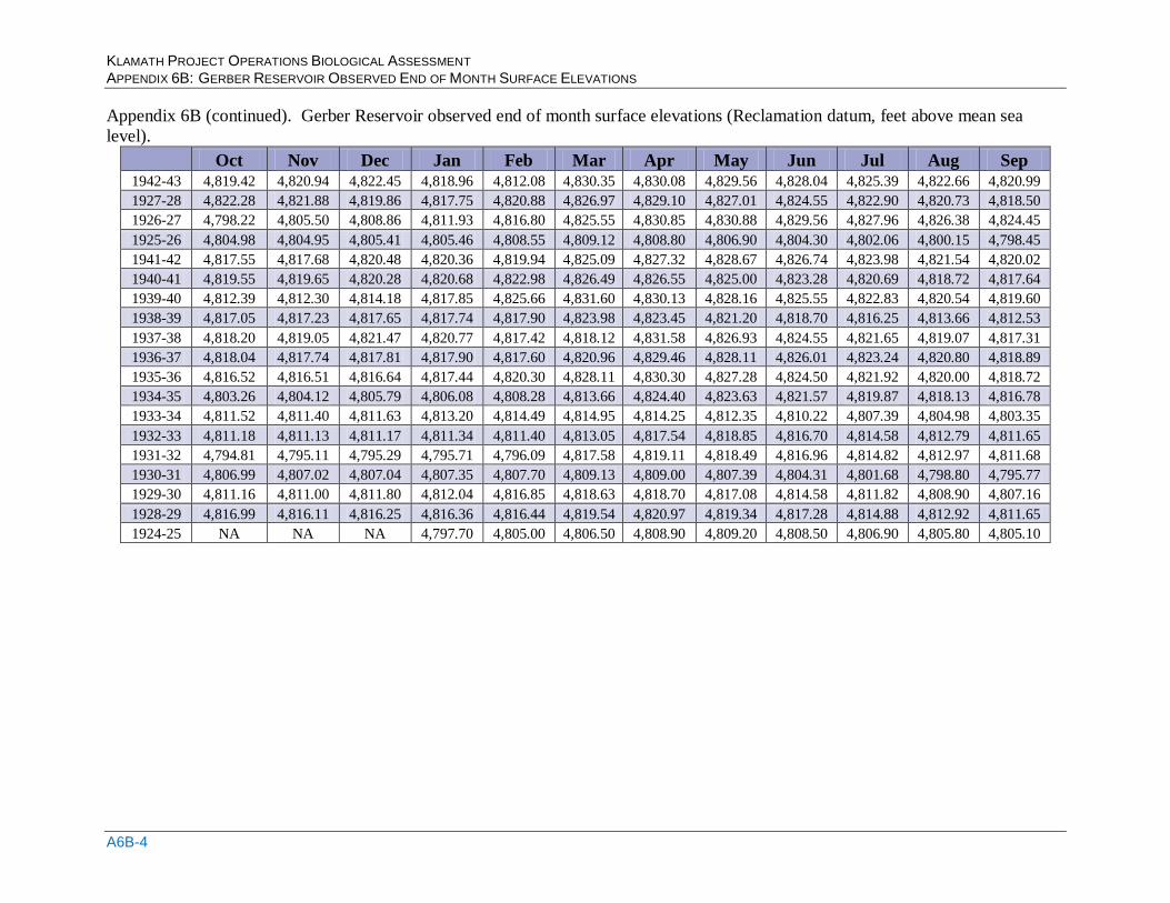
KLAMATH PROJECT OPERATIONS BIOLOGICAL ASSESSMENT APPENDIX 6B: GERBER RESERVOIR OBSERVED END OF MONTH SURFACE ELEVATIONS
A6B-4
Appendix 6B (continued). Gerber Reservoir observed end of month surface elevations (Reclamation datum, feet above mean sea
level).
Oct Nov Dec Jan Feb Mar Apr May Jun Jul Aug Sep
1942-43 4,819.42 4,820.94 4,822.45 4,818.96 4,812.08 4,830.35 4,830.08 4,829.56 4,828.04 4,825.39 4,822.66 4,820.99
1927-28 4,822.28 4,821.88 4,819.86 4,817.75 4,820.88 4,826.97 4,829.10 4,827.01 4,824.55 4,822.90 4,820.73 4,818.50
1926-27 4,798.22 4,805.50 4,808.86 4,811.93 4,816.80 4,825.55 4,830.85 4,830.88 4,829.56 4,827.96 4,826.38 4,824.45
1925-26 4,804.98 4,804.95 4,805.41 4,805.46 4,808.55 4,809.12 4,808.80 4,806.90 4,804.30 4,802.06 4,800.15 4,798.45
1941-42 4,817.55 4,817.68 4,820.48 4,820.36 4,819.94 4,825.09 4,827.32 4,828.67 4,826.74 4,823.98 4,821.54 4,820.02
1940-41 4,819.55 4,819.65 4,820.28 4,820.68 4,822.98 4,826.49 4,826.55 4,825.00 4,823.28 4,820.69 4,818.72 4,817.64
1939-40 4,812.39 4,812.30 4,814.18 4,817.85 4,825.66 4,831.60 4,830.13 4,828.16 4,825.55 4,822.83 4,820.54 4,819.60
1938-39 4,817.05 4,817.23 4,817.65 4,817.74 4,817.90 4,823.98 4,823.45 4,821.20 4,818.70 4,816.25 4,813.66 4,812.53
1937-38 4,818.20 4,819.05 4,821.47 4,820.77 4,817.42 4,818.12 4,831.58 4,826.93 4,824.55 4,821.65 4,819.07 4,817.31
1936-37 4,818.04 4,817.74 4,817.81 4,817.90 4,817.60 4,820.96 4,829.46 4,828.11 4,826.01 4,823.24 4,820.80 4,818.89
1935-36 4,816.52 4,816.51 4,816.64 4,817.44 4,820.30 4,828.11 4,830.30 4,827.28 4,824.50 4,821.92 4,820.00 4,818.72
1934-35 4,803.26 4,804.12 4,805.79 4,806.08 4,808.28 4,813.66 4,824.40 4,823.63 4,821.57 4,819.87 4,818.13 4,816.78
1933-34 4,811.52 4,811.40 4,811.63 4,813.20 4,814.49 4,814.95 4,814.25 4,812.35 4,810.22 4,807.39 4,804.98 4,803.35
1932-33 4,811.18 4,811.13 4,811.17 4,811.34 4,811.40 4,813.05 4,817.54 4,818.85 4,816.70 4,814.58 4,812.79 4,811.65
1931-32 4,794.81 4,795.11 4,795.29 4,795.71 4,796.09 4,817.58 4,819.11 4,818.49 4,816.96 4,814.82 4,812.97 4,811.68
1930-31 4,806.99 4,807.02 4,807.04 4,807.35 4,807.70 4,809.13 4,809.00 4,807.39 4,804.31 4,801.68 4,798.80 4,795.77
1929-30 4,811.16 4,811.00 4,811.80 4,812.04 4,816.85 4,818.63 4,818.70 4,817.08 4,814.58 4,811.82 4,808.90 4,807.16
1928-29 4,816.99 4,816.11 4,816.25 4,816.36 4,816.44 4,819.54 4,820.97 4,819.34 4,817.28 4,814.88 4,812.92 4,811.65
1924-25 NA NA NA 4,797.70 4,805.00 4,806.50 4,808.90 4,809.20 4,808.50 4,806.90 4,805.80 4,805.10

KLAMATH PROJECT OPERATIONS BIOLOGICAL ASSESSMENT APPENDIX 8A: KLAMATH COHO SALMON
Appendix 8A: Coho Salmon

KLAMATH PROJECT OPERATIONS BIOLOGICAL ASSESSMENT APPENDIX 8A: KLAMATH COHO SALMON
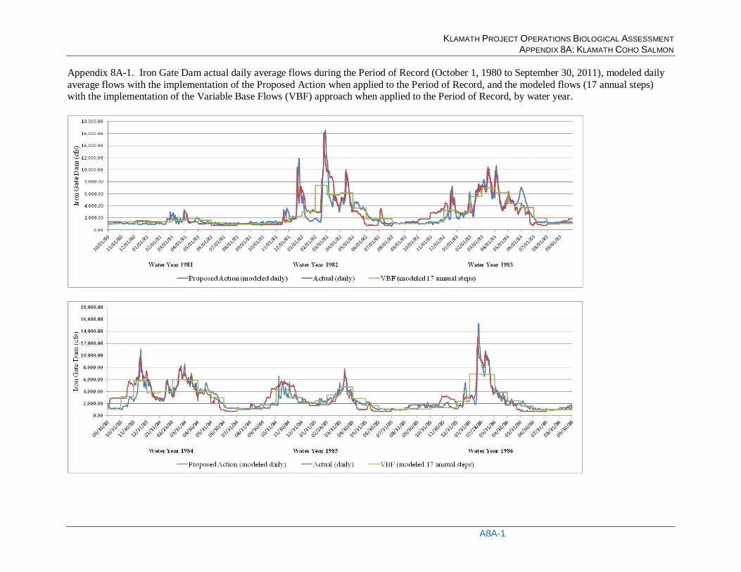
KLAMATH PROJECT OPERATIONS BIOLOGICAL ASSESSMENT APPENDIX 8A: KLAMATH COHO SALMON
A8A-1
Appendix 8A-1. Iron Gate Dam actual daily average flows during the Period of Record (October 1, 1980 to September 30, 2011), modeled daily
average flows with the implementation of the Proposed Action when applied to the Period of Record, and the modeled flows (17 annual steps) with the implementation of the Variable Base Flows (VBF) approach when applied to the Period of Record, by water year.
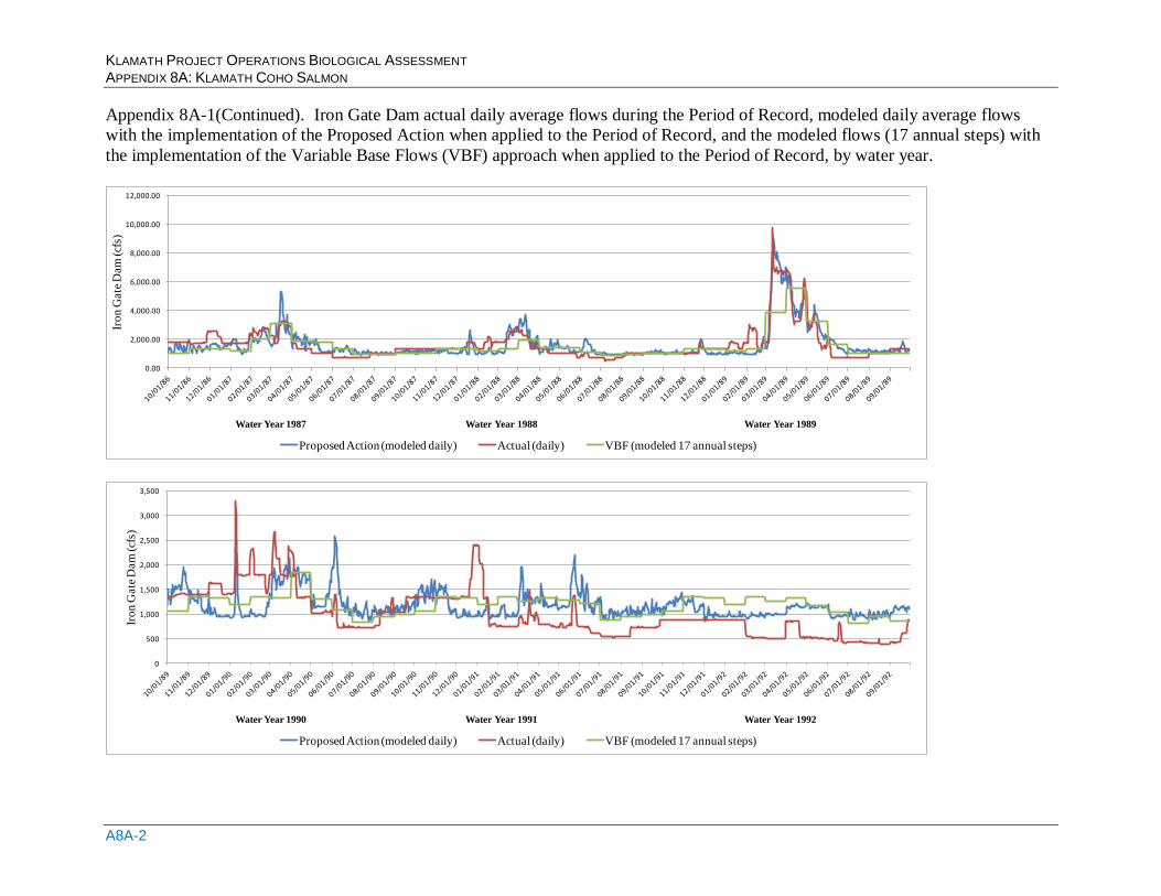
KLAMATH PROJECT OPERATIONS BIOLOGICAL ASSESSMENT APPENDIX 8A: KLAMATH COHO SALMON
A8A-2
Appendix 8A-1(Continued). Iron Gate Dam actual daily average flows during the Period of Record, modeled daily average flows
with the implementation of the Proposed Action when applied to the Period of Record, and the modeled flows (17 annual steps) with
the implementation of the Variable Base Flows (VBF) approach when applied to the Period of Record, by water year.
0.00
2,000.00
4,000.00
6,000.00
8,000.00
10,000.00
12,000.00
Iro
n G
ate
Dam
(cf
s)
Water Year 1987 Water Year 1988 Water Year 1989
Proposed Action (modeled daily) Actual (daily) VBF (modeled 17 annual steps)
0
500
1,000
1,500
2,000
2,500
3,000
3,500
Iro
n G
ate
Dam
(cf
s)
Water Year 1990 Water Year 1991 Water Year 1992
Proposed Action (modeled daily) Actual (daily) VBF (modeled 17 annual steps)
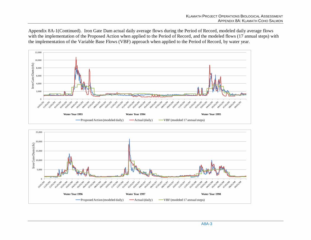
KLAMATH PROJECT OPERATIONS BIOLOGICAL ASSESSMENT APPENDIX 8A: KLAMATH COHO SALMON
A8A-3
Appendix 8A-1(Continued). Iron Gate Dam actual daily average flows during the Period of Record, modeled daily average flows
with the implementation of the Proposed Action when applied to the Period of Record, and the modeled flows (17 annual steps) with
the implementation of the Variable Base Flows (VBF) approach when applied to the Period of Record, by water year.
0
2,000
4,000
6,000
8,000
10,000
12,000
Iro
n G
ate
Dam
(cf
s)
Water Year 1993 Water Year 1994 Water Year 1995
Proposed Action (modeled daily) Actual (daily) VBF (modeled 17 annual steps)
0
5,000
10,000
15,000
20,000
25,000
Iro
n G
ate
Dam
(cf
s)
Water Year 1996 Water Year 1997 Water Year 1998
Proposed Action (modeled daily) Actual (daily) VBF (modeled 17 annual steps)
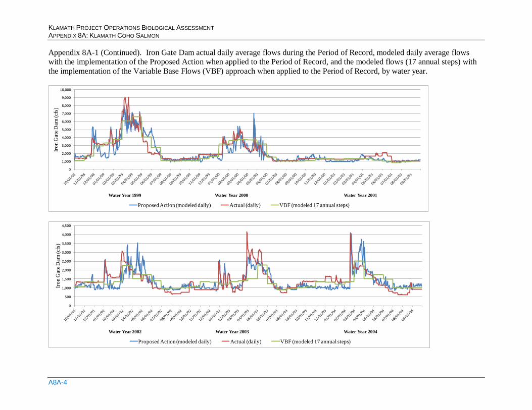
KLAMATH PROJECT OPERATIONS BIOLOGICAL ASSESSMENT APPENDIX 8A: KLAMATH COHO SALMON
A8A-4
Appendix 8A-1 (Continued). Iron Gate Dam actual daily average flows during the Period of Record, modeled daily average flows
with the implementation of the Proposed Action when applied to the Period of Record, and the modeled flows (17 annual steps) with
the implementation of the Variable Base Flows (VBF) approach when applied to the Period of Record, by water year.
0
1,000
2,000
3,000
4,000
5,000
6,000
7,000
8,000
9,000
10,000
Iro
n G
ate
Dam
(cf
s)
Water Year 1999 Water Year 2000 Water Year 2001
Proposed Action (modeled daily) Actual (daily) VBF (modeled 17 annual steps)
0
500
1,000
1,500
2,000
2,500
3,000
3,500
4,000
4,500
Iro
n G
ate
Dam
(cf
s)
Water Year 2002 Water Year 2003 Water Year 2004
Proposed Action (modeled daily) Actual (daily) VBF (modeled 17 annual steps)
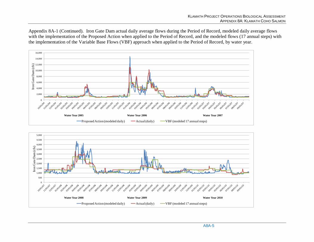
KLAMATH PROJECT OPERATIONS BIOLOGICAL ASSESSMENT APPENDIX 8A: KLAMATH COHO SALMON
A8A-5
Appendix 8A-1 (Continued). Iron Gate Dam actual daily average flows during the Period of Record, modeled daily average flows
with the implementation of the Proposed Action when applied to the Period of Record, and the modeled flows (17 annual steps) with
the implementation of the Variable Base Flows (VBF) approach when applied to the Period of Record, by water year.
0
2,000
4,000
6,000
8,000
10,000
12,000
14,000
16,000
Iro
n G
ate
Dam
(cf
s)
Water Year 2005 Water Year 2006 Water Year 2007
Proposed Action (modeled daily) Actual (daily) VBF (modeled 17 annual steps)
0
500
1,000
1,500
2,000
2,500
3,000
3,500
4,000
4,500
5,000
Iro
n G
ate
Dam
(cf
s)
Water Year 2008 Water Year 2009 Water Year 2010
Proposed Action (modeled daily) Actual (daily) VBF (modeled 17 annual steps)
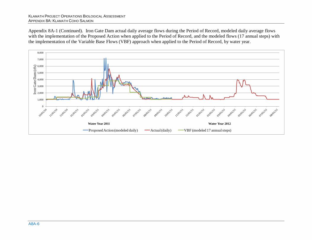
KLAMATH PROJECT OPERATIONS BIOLOGICAL ASSESSMENT APPENDIX 8A: KLAMATH COHO SALMON
A8A-6
Appendix 8A-1 (Continued). Iron Gate Dam actual daily average flows during the Period of Record, modeled daily average flows
with the implementation of the Proposed Action when applied to the Period of Record, and the modeled flows (17 annual steps) with
the implementation of the Variable Base Flows (VBF) approach when applied to the Period of Record, by water year.
0
1,000
2,000
3,000
4,000
5,000
6,000
7,000
8,000
Iro
n G
ate
Dam
(cf
s)
Water Year 2011 Water Year 2012
Proposed Action (modeled daily) Actual (daily) VBF (modeled 17 annual steps)
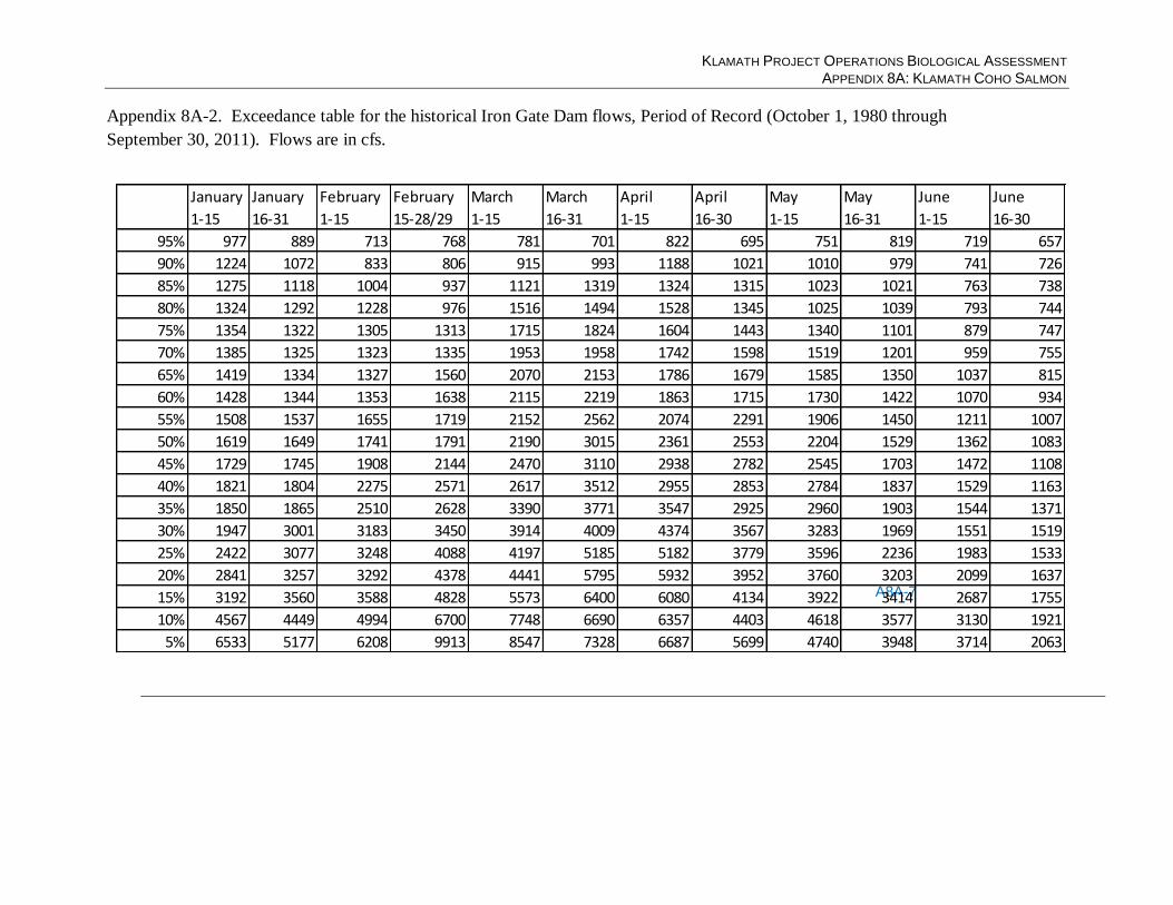
KLAMATH PROJECT OPERATIONS BIOLOGICAL ASSESSMENT APPENDIX 8A: KLAMATH COHO SALMON
A8A-7
Appendix 8A-2. Exceedance table for the historical Iron Gate Dam flows, Period of Record (October 1, 1980 through
September 30, 2011). Flows are in cfs.
January
1-15
January
16-31
February
1-15
February
15-28/29
March
1-15
March
16-31
April
1-15
April
16-30
May
1-15
May
16-31
June
1-15
June
16-30
95% 977 889 713 768 781 701 822 695 751 819 719 657
90% 1224 1072 833 806 915 993 1188 1021 1010 979 741 726
85% 1275 1118 1004 937 1121 1319 1324 1315 1023 1021 763 738
80% 1324 1292 1228 976 1516 1494 1528 1345 1025 1039 793 744
75% 1354 1322 1305 1313 1715 1824 1604 1443 1340 1101 879 747
70% 1385 1325 1323 1335 1953 1958 1742 1598 1519 1201 959 755
65% 1419 1334 1327 1560 2070 2153 1786 1679 1585 1350 1037 815
60% 1428 1344 1353 1638 2115 2219 1863 1715 1730 1422 1070 934
55% 1508 1537 1655 1719 2152 2562 2074 2291 1906 1450 1211 1007
50% 1619 1649 1741 1791 2190 3015 2361 2553 2204 1529 1362 1083
45% 1729 1745 1908 2144 2470 3110 2938 2782 2545 1703 1472 1108
40% 1821 1804 2275 2571 2617 3512 2955 2853 2784 1837 1529 1163
35% 1850 1865 2510 2628 3390 3771 3547 2925 2960 1903 1544 1371
30% 1947 3001 3183 3450 3914 4009 4374 3567 3283 1969 1551 1519
25% 2422 3077 3248 4088 4197 5185 5182 3779 3596 2236 1983 1533
20% 2841 3257 3292 4378 4441 5795 5932 3952 3760 3203 2099 1637
15% 3192 3560 3588 4828 5573 6400 6080 4134 3922 3414 2687 1755
10% 4567 4449 4994 6700 7748 6690 6357 4403 4618 3577 3130 1921
5% 6533 5177 6208 9913 8547 7328 6687 5699 4740 3948 3714 2063
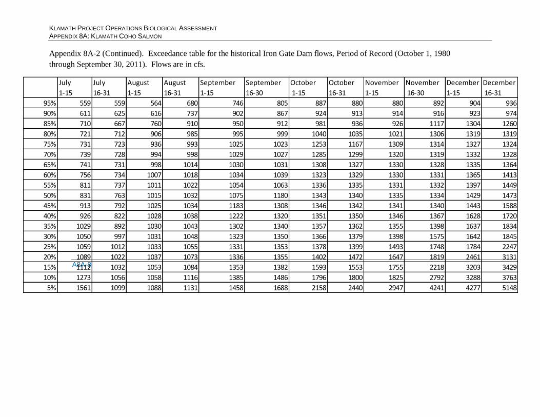
KLAMATH PROJECT OPERATIONS BIOLOGICAL ASSESSMENT APPENDIX 8A: KLAMATH COHO SALMON
A8A-8
Appendix 8A-2 (Continued). Exceedance table for the historical Iron Gate Dam flows, Period of Record (October 1, 1980
through September 30, 2011). Flows are in cfs.
July
1-15
July
16-31
August
1-15
August
16-31
September
1-15
September
16-30
October
1-15
October
16-31
November
1-15
November
16-30
December
1-15
December
16-31
95% 559 559 564 680 746 805 887 880 880 892 904 936
90% 611 625 616 737 902 867 924 913 914 916 923 974
85% 710 667 760 910 950 912 981 936 926 1117 1304 1260
80% 721 712 906 985 995 999 1040 1035 1021 1306 1319 1319
75% 731 723 936 993 1025 1023 1253 1167 1309 1314 1327 1324
70% 739 728 994 998 1029 1027 1285 1299 1320 1319 1332 1328
65% 741 731 998 1014 1030 1031 1308 1327 1330 1328 1335 1364
60% 756 734 1007 1018 1034 1039 1323 1329 1330 1331 1365 1413
55% 811 737 1011 1022 1054 1063 1336 1335 1331 1332 1397 1449
50% 831 763 1015 1032 1075 1180 1343 1340 1335 1334 1429 1473
45% 913 792 1025 1034 1183 1308 1346 1342 1341 1340 1443 1588
40% 926 822 1028 1038 1222 1320 1351 1350 1346 1367 1628 1720
35% 1029 892 1030 1043 1302 1340 1357 1362 1355 1398 1637 1834
30% 1050 997 1031 1048 1323 1350 1366 1379 1398 1575 1642 1845
25% 1059 1012 1033 1055 1331 1353 1378 1399 1493 1748 1784 2247
20% 1089 1022 1037 1073 1336 1355 1402 1472 1647 1819 2461 3131
15% 1112 1032 1053 1084 1353 1382 1593 1553 1755 2218 3203 3429
10% 1273 1056 1058 1116 1385 1486 1796 1800 1825 2792 3288 3763
5% 1561 1099 1088 1131 1458 1688 2158 2440 2947 4241 4277 5148
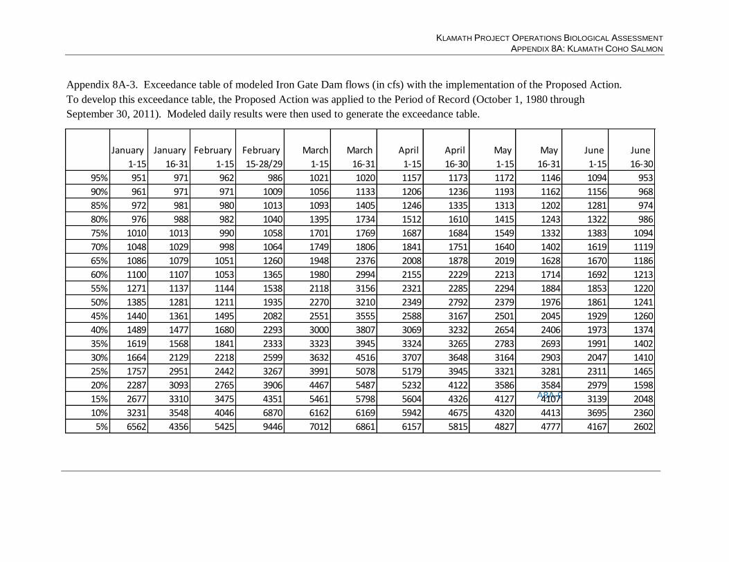
KLAMATH PROJECT OPERATIONS BIOLOGICAL ASSESSMENT APPENDIX 8A: KLAMATH COHO SALMON
A8A-9
Appendix 8A-3. Exceedance table of modeled Iron Gate Dam flows (in cfs) with the implementation of the Proposed Action.
To develop this exceedance table, the Proposed Action was applied to the Period of Record (October 1, 1980 through
September 30, 2011). Modeled daily results were then used to generate the exceedance table.
January January February February March March April April May May June June
1-15 16-31 1-15 15-28/29 1-15 16-31 1-15 16-30 1-15 16-31 1-15 16-30
95% 951 971 962 986 1021 1020 1157 1173 1172 1146 1094 953
90% 961 971 971 1009 1056 1133 1206 1236 1193 1162 1156 968
85% 972 981 980 1013 1093 1405 1246 1335 1313 1202 1281 974
80% 976 988 982 1040 1395 1734 1512 1610 1415 1243 1322 986
75% 1010 1013 990 1058 1701 1769 1687 1684 1549 1332 1383 1094
70% 1048 1029 998 1064 1749 1806 1841 1751 1640 1402 1619 1119
65% 1086 1079 1051 1260 1948 2376 2008 1878 2019 1628 1670 1186
60% 1100 1107 1053 1365 1980 2994 2155 2229 2213 1714 1692 1213
55% 1271 1137 1144 1538 2118 3156 2321 2285 2294 1884 1853 1220
50% 1385 1281 1211 1935 2270 3210 2349 2792 2379 1976 1861 1241
45% 1440 1361 1495 2082 2551 3555 2588 3167 2501 2045 1929 1260 40% 1489 1477 1680 2293 3000 3807 3069 3232 2654 2406 1973 1374
35% 1619 1568 1841 2333 3323 3945 3324 3265 2783 2693 1991 1402
30% 1664 2129 2218 2599 3632 4516 3707 3648 3164 2903 2047 1410
25% 1757 2951 2442 3267 3991 5078 5179 3945 3321 3281 2311 1465
20% 2287 3093 2765 3906 4467 5487 5232 4122 3586 3584 2979 1598
15% 2677 3310 3475 4351 5461 5798 5604 4326 4127 4107 3139 2048
10% 3231 3548 4046 6870 6162 6169 5942 4675 4320 4413 3695 2360
5% 6562 4356 5425 9446 7012 6861 6157 5815 4827 4777 4167 2602
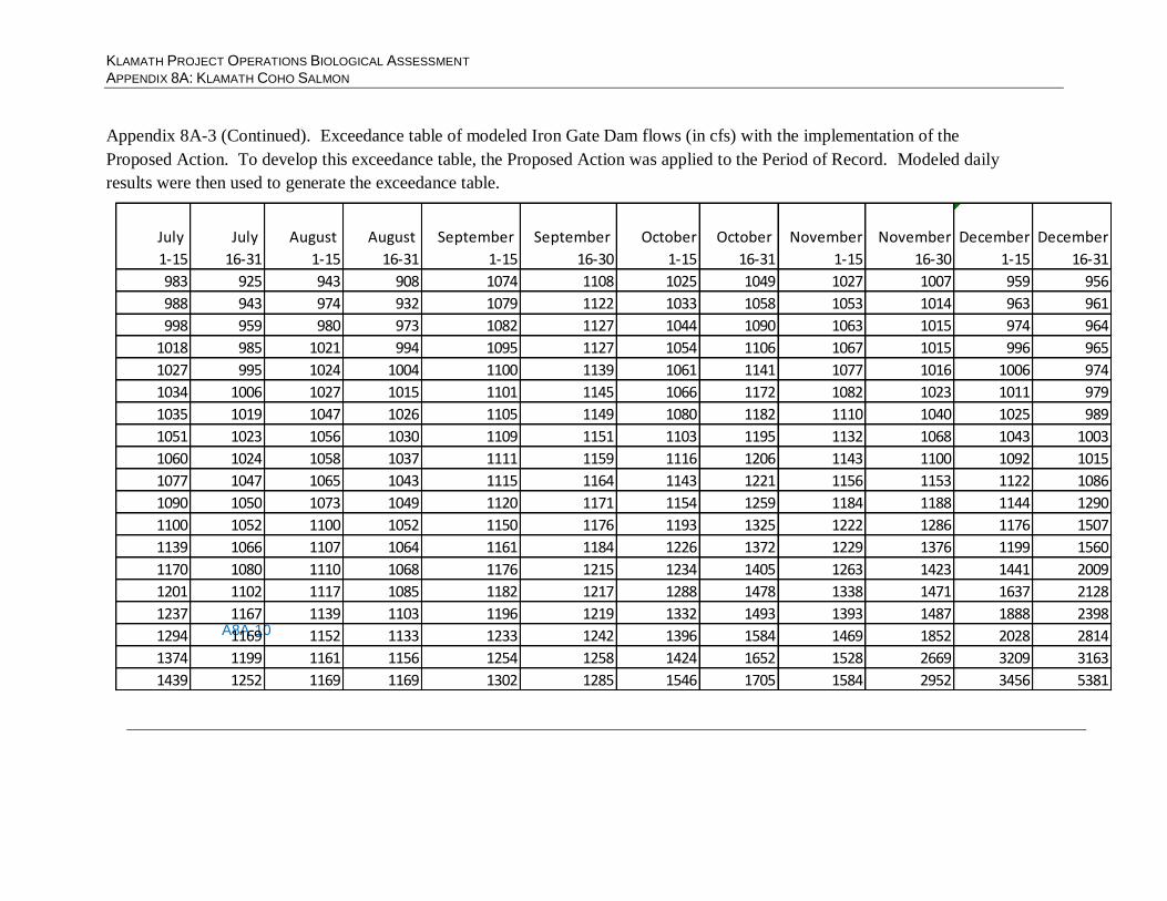
KLAMATH PROJECT OPERATIONS BIOLOGICAL ASSESSMENT APPENDIX 8A: KLAMATH COHO SALMON
A8A-10
Appendix 8A-3 (Continued). Exceedance table of modeled Iron Gate Dam flows (in cfs) with the implementation of the
Proposed Action. To develop this exceedance table, the Proposed Action was applied to the Period of Record. Modeled daily
results were then used to generate the exceedance table.
July July August August September September October October November November December December
1-15 16-31 1-15 16-31 1-15 16-30 1-15 16-31 1-15 16-30 1-15 16-31
983 925 943 908 1074 1108 1025 1049 1027 1007 959 956
988 943 974 932 1079 1122 1033 1058 1053 1014 963 961
998 959 980 973 1082 1127 1044 1090 1063 1015 974 964
1018 985 1021 994 1095 1127 1054 1106 1067 1015 996 965
1027 995 1024 1004 1100 1139 1061 1141 1077 1016 1006 974
1034 1006 1027 1015 1101 1145 1066 1172 1082 1023 1011 979
1035 1019 1047 1026 1105 1149 1080 1182 1110 1040 1025 989
1051 1023 1056 1030 1109 1151 1103 1195 1132 1068 1043 1003
1060 1024 1058 1037 1111 1159 1116 1206 1143 1100 1092 1015
1077 1047 1065 1043 1115 1164 1143 1221 1156 1153 1122 1086
1090 1050 1073 1049 1120 1171 1154 1259 1184 1188 1144 1290
1100 1052 1100 1052 1150 1176 1193 1325 1222 1286 1176 1507
1139 1066 1107 1064 1161 1184 1226 1372 1229 1376 1199 1560
1170 1080 1110 1068 1176 1215 1234 1405 1263 1423 1441 2009
1201 1102 1117 1085 1182 1217 1288 1478 1338 1471 1637 2128
1237 1167 1139 1103 1196 1219 1332 1493 1393 1487 1888 2398
1294 1169 1152 1133 1233 1242 1396 1584 1469 1852 2028 2814
1374 1199 1161 1156 1254 1258 1424 1652 1528 2669 3209 3163
1439 1252 1169 1169 1302 1285 1546 1705 1584 2952 3456 5381
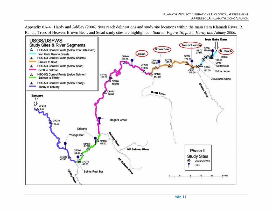
KLAMATH PROJECT OPERATIONS BIOLOGICAL ASSESSMENT APPENDIX 8A: KLAMATH COHO SALMON
A8A-11
Appendix 8A-4. Hardy and Addley (2006) river reach delineations and study site locations within the main stem Klamath River. R.
Ranch, Trees of Heaven, Brown Bear, and Seiad study sites are highlighted. Source: Figure 16, p. 54, Hardy and Addley 2006.
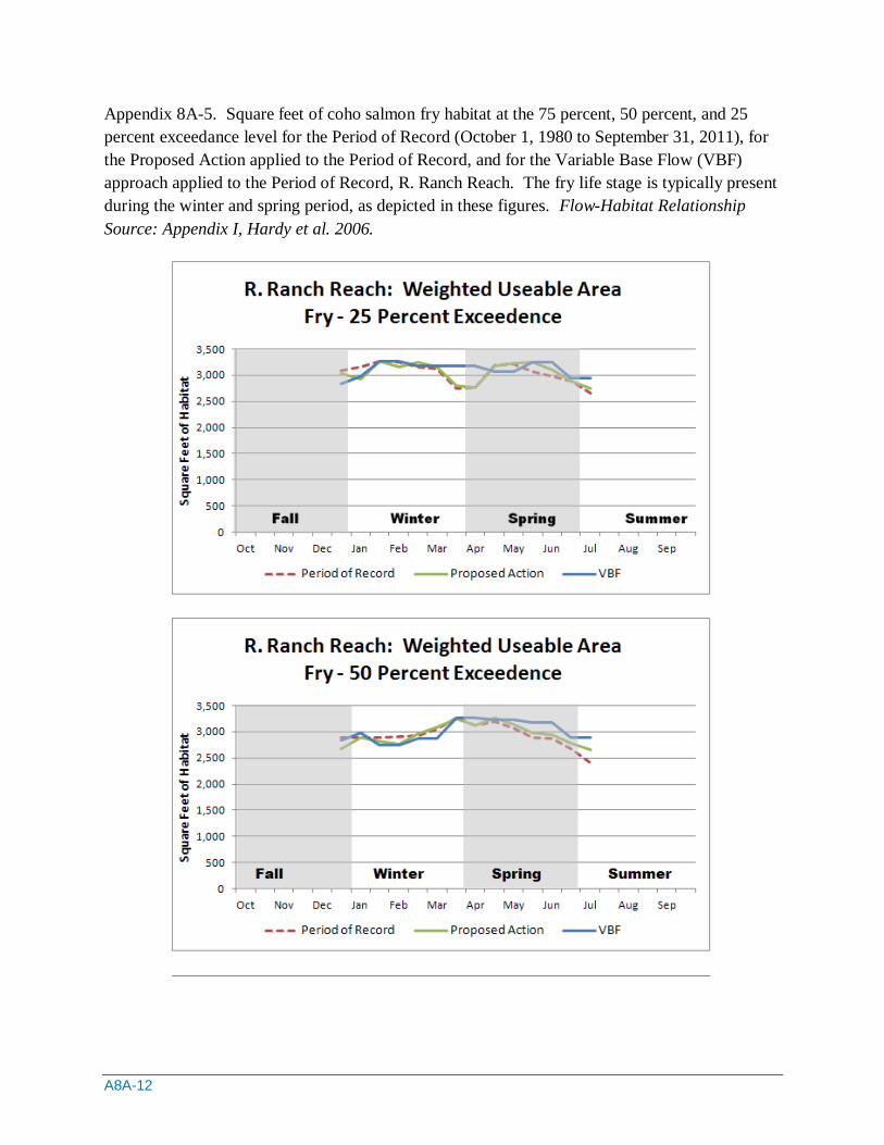
A8A-12
Appendix 8A-5. Square feet of coho salmon fry habitat at the 75 percent, 50 percent, and 25
percent exceedance level for the Period of Record (October 1, 1980 to September 31, 2011), for
the Proposed Action applied to the Period of Record, and for the Variable Base Flow (VBF)
approach applied to the Period of Record, R. Ranch Reach. The fry life stage is typically present
during the winter and spring period, as depicted in these figures. Flow-Habitat Relationship
Source: Appendix I, Hardy et al. 2006.
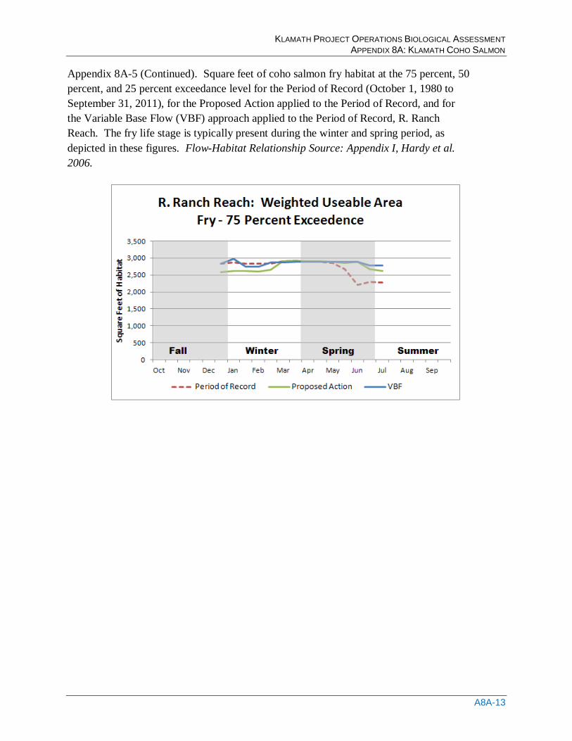
KLAMATH PROJECT OPERATIONS BIOLOGICAL ASSESSMENT APPENDIX 8A: KLAMATH COHO SALMON
A8A-13
Appendix 8A-5 (Continued). Square feet of coho salmon fry habitat at the 75 percent, 50
percent, and 25 percent exceedance level for the Period of Record (October 1, 1980 to
September 31, 2011), for the Proposed Action applied to the Period of Record, and for
the Variable Base Flow (VBF) approach applied to the Period of Record, R. Ranch
Reach. The fry life stage is typically present during the winter and spring period, as
depicted in these figures. Flow-Habitat Relationship Source: Appendix I, Hardy et al.
2006.
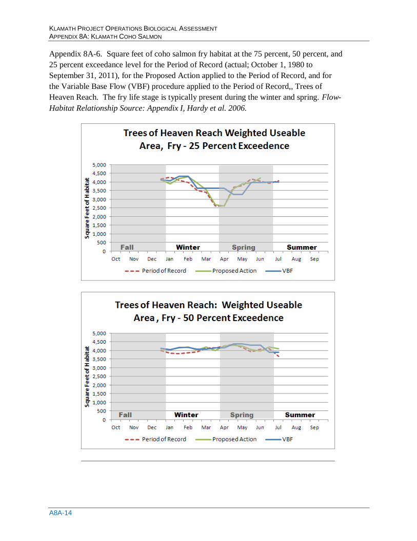
KLAMATH PROJECT OPERATIONS BIOLOGICAL ASSESSMENT APPENDIX 8A: KLAMATH COHO SALMON
A8A-14
Appendix 8A-6. Square feet of coho salmon fry habitat at the 75 percent, 50 percent, and
25 percent exceedance level for the Period of Record (actual; October 1, 1980 to
September 31, 2011), for the Proposed Action applied to the Period of Record, and for
the Variable Base Flow (VBF) procedure applied to the Period of Record,, Trees of
Heaven Reach. The fry life stage is typically present during the winter and spring. Flow-
Habitat Relationship Source: Appendix I, Hardy et al. 2006.
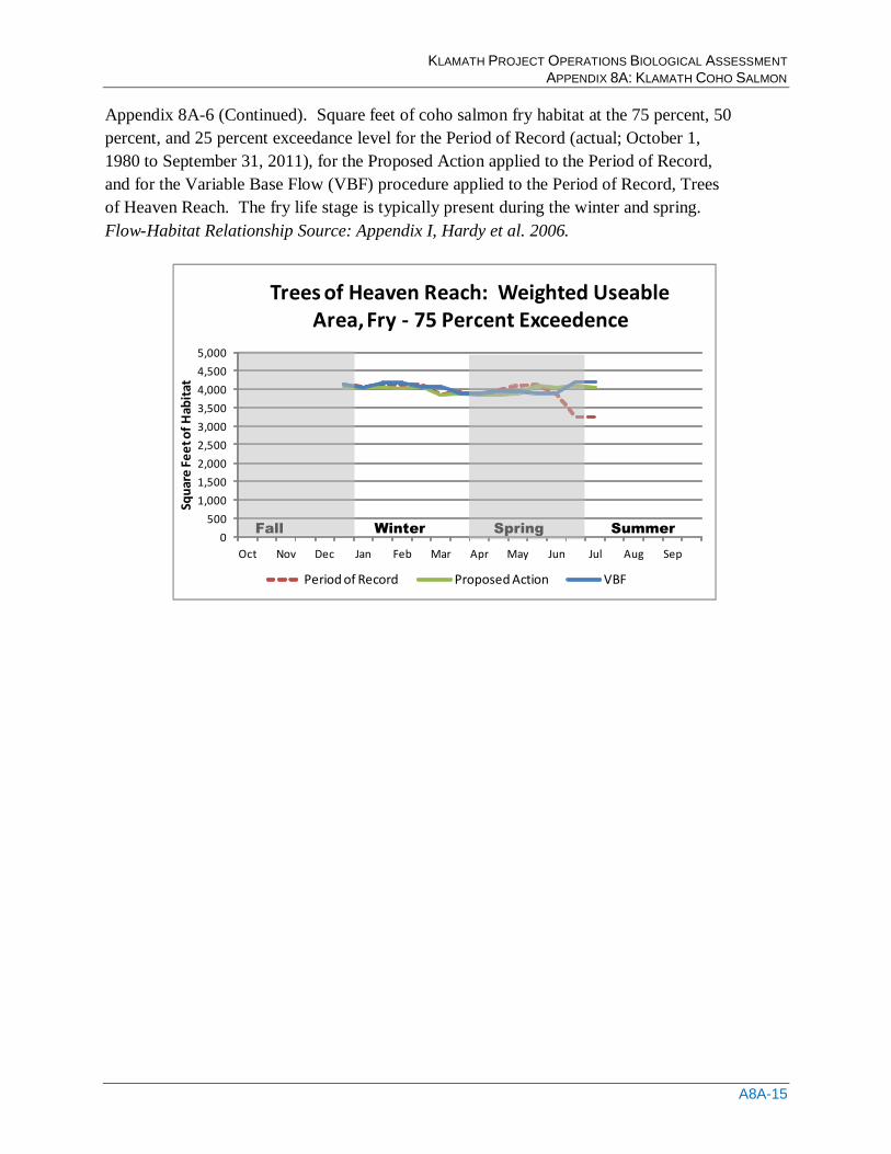
KLAMATH PROJECT OPERATIONS BIOLOGICAL ASSESSMENT APPENDIX 8A: KLAMATH COHO SALMON
A8A-15
Appendix 8A-6 (Continued). Square feet of coho salmon fry habitat at the 75 percent, 50
percent, and 25 percent exceedance level for the Period of Record (actual; October 1,
1980 to September 31, 2011), for the Proposed Action applied to the Period of Record,
and for the Variable Base Flow (VBF) procedure applied to the Period of Record, Trees
of Heaven Reach. The fry life stage is typically present during the winter and spring.
Flow-Habitat Relationship Source: Appendix I, Hardy et al. 2006.
0
500
1,000
1,500
2,000
2,500
3,000
3,500
4,000
4,500
5,000
Oct Nov Dec Jan Feb Mar Apr May Jun Jul Aug Sep
Squ
are
Fe
et o
f H
abit
at
Trees of Heaven Reach: Weighted Useable Area, Fry - 75 Percent Exceedence
Period of Record Proposed Action VBF
Fall Winter Spring Summer
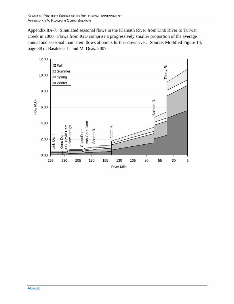
KLAMATH PROJECT OPERATIONS BIOLOGICAL ASSESSMENT APPENDIX 8A: KLAMATH COHO SALMON
A8A-16
Appendix 8A-7. Simulated seasonal flows in the Klamath River from Link River to Turwar
Creek in 2000. Flows from IGD comprise a progressively smaller proportion of the average
annual and seasonal main stem flows at points further downriver. Source: Modified Figure 14,
page 88 of Basdekas L. and M. Deas. 2007.
0.00
2.00
4.00
6.00
8.00
10.00
12.00
5305580105130155180205230255
River Mile
Flo
w M
AF
Fall
Summer
Spring
Winter
Trinity R
.
Salm
on R
.
Scott
R.
Shasta
R.
Iron G
ate
Dam
J.C
. B
oyle
Dam
Keno D
am
Lin
k D
am
CopcoD
am
belo
w s
prings
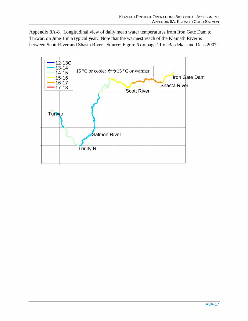
KLAMATH PROJECT OPERATIONS BIOLOGICAL ASSESSMENT APPENDIX 8A: KLAMATH COHO SALMON
A8A-17
Appendix 8A-8. Longitudinal view of daily mean water temperatures from Iron Gate Dam to
Turwar, on June 1 in a typical year. Note that the warmest reach of the Klamath River is
between Scott River and Shasta River. Source: Figure 6 on page 11 of Basdekas and Deas 2007.
12-13C 13-14 14-15 15-16 16-17 17-18
Iron Gate Dam
Shasta River .
Scott River .
Salmon River .
Trinity R .
Turwar
15 C or cooler 15 C or warmer
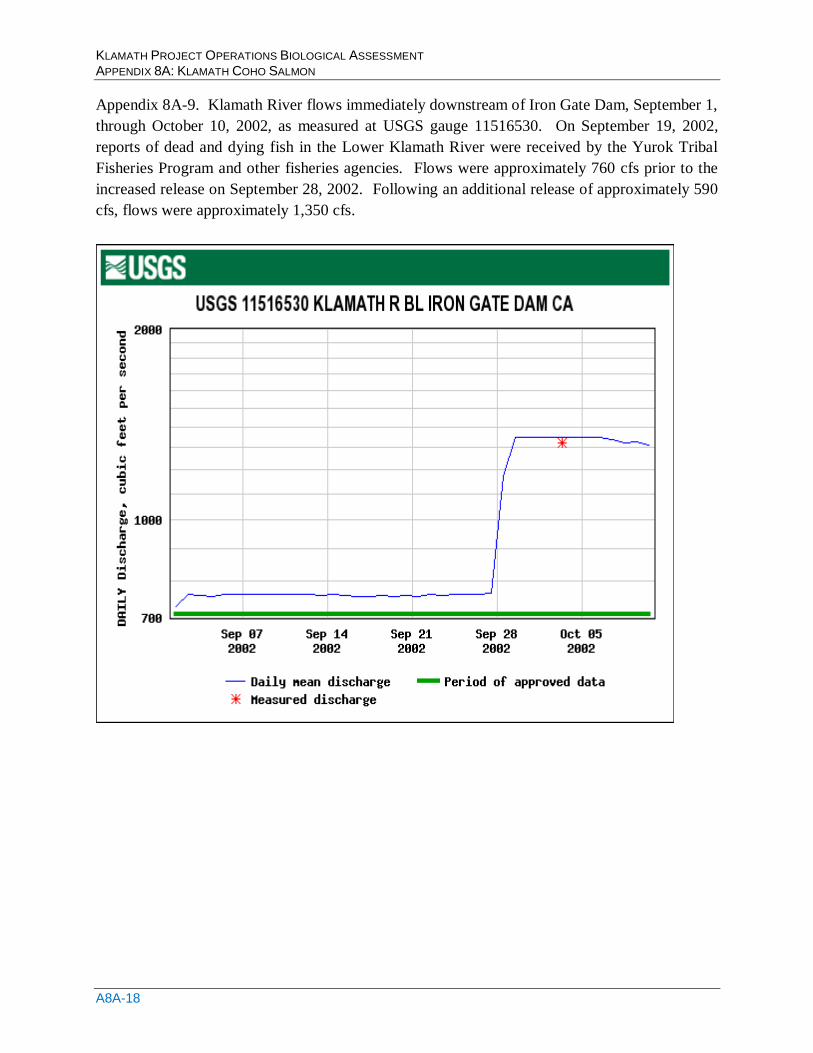
KLAMATH PROJECT OPERATIONS BIOLOGICAL ASSESSMENT APPENDIX 8A: KLAMATH COHO SALMON
A8A-18
Appendix 8A-9. Klamath River flows immediately downstream of Iron Gate Dam, September 1,
through October 10, 2002, as measured at USGS gauge 11516530. On September 19, 2002,
reports of dead and dying fish in the Lower Klamath River were received by the Yurok Tribal
Fisheries Program and other fisheries agencies. Flows were approximately 760 cfs prior to the
increased release on September 28, 2002. Following an additional release of approximately 590
cfs, flows were approximately 1,350 cfs.
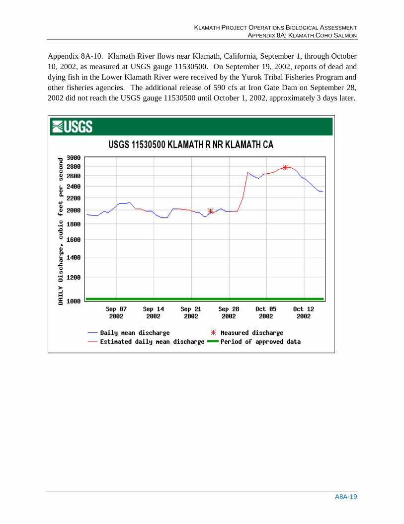
KLAMATH PROJECT OPERATIONS BIOLOGICAL ASSESSMENT APPENDIX 8A: KLAMATH COHO SALMON
A8A-19
Appendix 8A-10. Klamath River flows near Klamath, California, September 1, through October
10, 2002, as measured at USGS gauge 11530500. On September 19, 2002, reports of dead and
dying fish in the Lower Klamath River were received by the Yurok Tribal Fisheries Program and
other fisheries agencies. The additional release of 590 cfs at Iron Gate Dam on September 28,
2002 did not reach the USGS gauge 11530500 until October 1, 2002, approximately 3 days later.
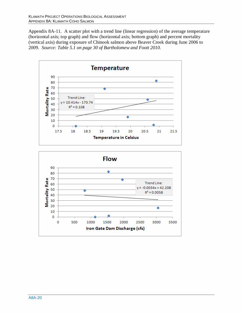
KLAMATH PROJECT OPERATIONS BIOLOGICAL ASSESSMENT APPENDIX 8A: KLAMATH COHO SALMON
A8A-20
Appendix 8A-11. A scatter plot with a trend line (linear regression) of the average temperature
(horizontal axis; top graph) and flow (horizontal axis; bottom graph) and percent mortality
(vertical axis) during exposure of Chinook salmon above Beaver Creek during June 2006 to
2009. Source: Table 5.1 on page 30 of Bartholomew and Foott 2010.
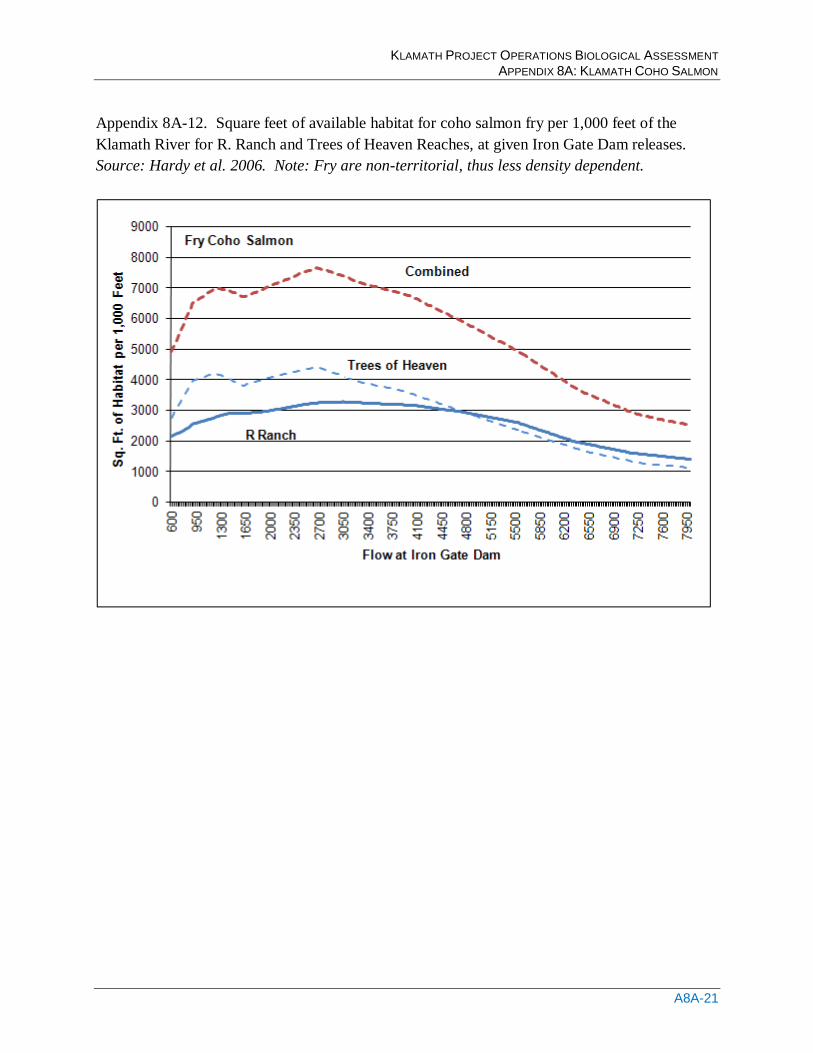
KLAMATH PROJECT OPERATIONS BIOLOGICAL ASSESSMENT APPENDIX 8A: KLAMATH COHO SALMON
A8A-21
Appendix 8A-12. Square feet of available habitat for coho salmon fry per 1,000 feet of the
Klamath River for R. Ranch and Trees of Heaven Reaches, at given Iron Gate Dam releases.
Source: Hardy et al. 2006. Note: Fry are non-territorial, thus less density dependent.
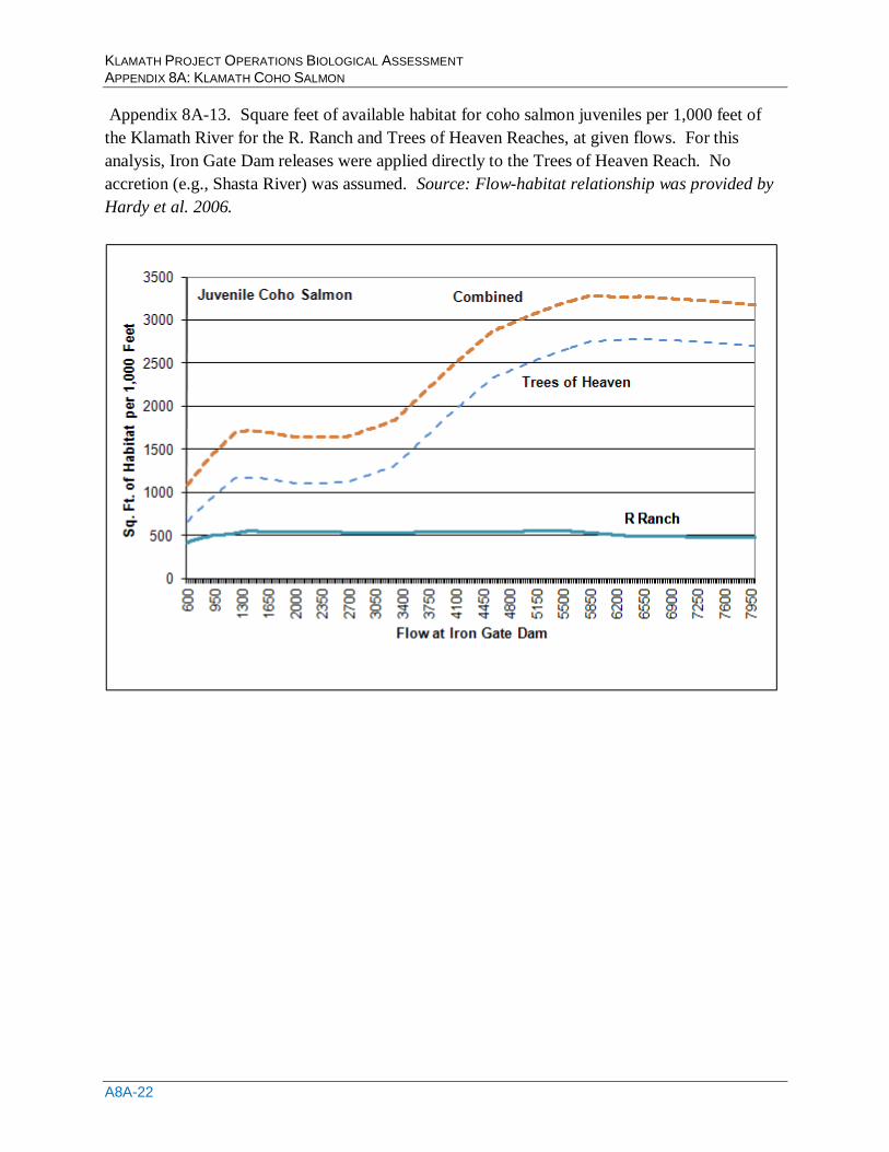
KLAMATH PROJECT OPERATIONS BIOLOGICAL ASSESSMENT APPENDIX 8A: KLAMATH COHO SALMON
A8A-22
Appendix 8A-13. Square feet of available habitat for coho salmon juveniles per 1,000 feet of
the Klamath River for the R. Ranch and Trees of Heaven Reaches, at given flows. For this
analysis, Iron Gate Dam releases were applied directly to the Trees of Heaven Reach. No
accretion (e.g., Shasta River) was assumed. Source: Flow-habitat relationship was provided by
Hardy et al. 2006.
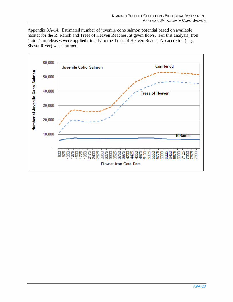
KLAMATH PROJECT OPERATIONS BIOLOGICAL ASSESSMENT APPENDIX 8A: KLAMATH COHO SALMON
A8A-23
Appendix 8A-14. Estimated number of juvenile coho salmon potential based on available
habitat for the R. Ranch and Trees of Heaven Reaches, at given flows. For this analysis, Iron
Gate Dam releases were applied directly to the Trees of Heaven Reach. No accretion (e.g.,
Shasta River) was assumed.

KLAMATH PROJECT OPERATIONS BIOLOGICAL ASSESSMENT APPENDIX 8A: KLAMATH COHO SALMON
A8A-24
Appendix 8A-15. Picture of a “dry” Link River on July 18, 1918 (Klamath County Museum).
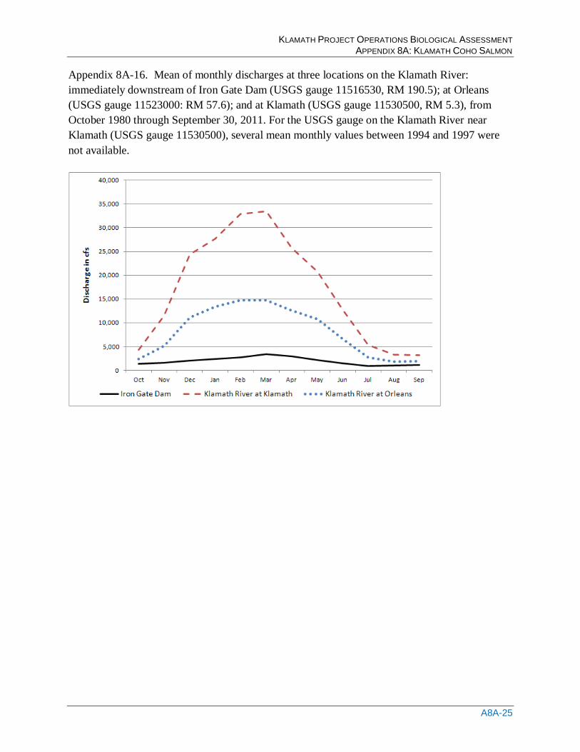
KLAMATH PROJECT OPERATIONS BIOLOGICAL ASSESSMENT APPENDIX 8A: KLAMATH COHO SALMON
A8A-25
Appendix 8A-16. Mean of monthly discharges at three locations on the Klamath River:
immediately downstream of Iron Gate Dam (USGS gauge 11516530, RM 190.5); at Orleans
(USGS gauge 11523000: RM 57.6); and at Klamath (USGS gauge 11530500, RM 5.3), from
October 1980 through September 30, 2011. For the USGS gauge on the Klamath River near
Klamath (USGS gauge 11530500), several mean monthly values between 1994 and 1997 were
not available.

KLAMATH PROJECT OPERATIONS BIOLOGICAL ASSESSMENT APPENDIX 8A: KLAMATH COHO SALMON
A8A-26
End of Appendix 8A

KLAMATH PROJECT OPERATIONS BIOLOGICAL ASSESSMENT APPENDIX 9A: OTHER SPECIES
Appendix 9A: Other Species

KLAMATH PROJECT OPERATIONS BIOLOGICAL ASSESSMENT APPENDIX 9A: OTHER SPECIES
KLAMATH PROJECT OPERATIONS BIOLOGICAL ASSESSMENT APPENDIX 9A: OTHER SPECIES
A9A-1
9A.1. Southern DPS North American Green Sturgeon 9A.1.1. Description Green sturgeon (Acipenser medirostris) are long-lived, slow-growing fish and the most marine-oriented of the sturgeon species. Males at maturity range from 4.5 to 6.5 feet (1.4 to 2 m) in fork length and are at least 15 years old (VanEenennaam 2002), while mature females range from 5 to 7 feet (1.6 to 2.2 m) fork length and are at least 17 years old. Adult green sturgeon maximum ages likely range from 60 to 70 years (Moyle 2002). This species is found along the west coast of Mexico, the United States, and Canada. Green sturgeon are members of the class of bony fishes, and the skeleton is composed mostly of cartilage. Sturgeon lack scales; however, they have five rows of characteristic bony plates on their body called scutes. The green sturgeon backbone curves upward into the caudal fin, forming their shark-like tail. On the ventral, or underside, of their flattened snouts are sensory barbels and a siphon-shaped, protrusible, toothless mouth. Recent genetic information suggests that green sturgeon in North America are taxonomically distinct from morphologically similar forms in Asia. 9A.1.2. Life History Green sturgeon are believed to spend the majority of their lives in nearshore oceanic waters, bays, and estuaries. Early life-history stages reside in fresh water, with adults returning to freshwater to spawn when they are more than 15 years of age and more than 4 feet (1.3 m) in size. Spawning is believed to occur every 2-5 years (Moyle, 2002). Adults typically migrate into fresh water beginning in late February; spawning occurs from March-July, with peak activity from April-June (Moyle et al., 1995). Females produce 60,000-140,000 eggs (Moyle et al., 1992). Juvenile green sturgeon spend 1-4 years in fresh and estuarine waters before dispersal to saltwater (Beamsesderfer and Webb, 2002). They disperse widely in the ocean after their out-migration from freshwater (Moyle et al., 1992). Spawning: Green sturgeon spawn every three to five years (Tracy 1990). Their spawning period is March to July, with a peak in mid-April to mid-June (Moyle et al. 1992). Green sturgeon’s preferred spawning areas are associated with deep pools or “holes” in large, turbulent river mainstems (Moyle et al. 1992). Spawning habitat preferences are likely large cobble substrates, but may range from clean sand to bedrock substrates. Green sturgeon broadcast their eggs over the large cobble substrates where they settle into the interstitial spaces between cobbles. Green sturgeon females produce 60,000 to 140,000 eggs (Moyle et al. 1992) and they are the largest eggs (diameter 4.34 mm) of any sturgeon species (Cech et al. 2000). Temperatures above 20° C are lethal to green sturgeon embryos (Cech et al. 2000). Green sturgeon spawning has only been documented in the Klamath, Sacramento (Moyle et al. 1992, CDFG 2002) and Rogue (Erickson et al. 2001, Rien et al. 2001) rivers in recent times. The Klamath Basin is thought to support the largest green sturgeon spawning population (Moyle et al. 1992). In the Klamath River, sturgeon courtship behaviors such as breaching have been observed in “The Sturgeon Hole” upstream of Orleans, CA (rkm 96). Larvae and juveniles have been caught in the Karuk Tribe’s Big Bar trap (rkm 80) on the Klamath and in the Willow Creek trap (rkm 40) on the Trinity River. In the Sacramento River, green sturgeon spawn in late spring

KLAMATH PROJECT OPERATIONS BIOLOGICAL ASSESSMENT APPENDIX 9A: OTHER SPECIES
A9A-2
and early summer above Hamilton City and perhaps as far upstream as Keswick Dam (CDFG 2002). Green sturgeon spawning has also been documented in the Rogue River (Erickson et al. 2001, Rien et al. 2001, NMFS 2005). Early Life History: Green sturgeon larvae first feed at 10 days post hatch, and metamorphosis to the juvenile stage is complete at 45 days. Larvae grow fast, reaching a length of 66 mm and a weight of 1.8 g in 3 weeks of exogenous feeding. Juveniles averaged 29 mm at the peak of occurrence in June/July at the Red Bluff Diversion Dam (California) fish trap and 36 mm at their peak abundance in July at the GCID trap (NMFS 2005a). These growth rates are consistent with rapid juvenile growth to 300 mm in 1 year and to over 600 mm within 2 to 3 years in the Klamath River (Nakamoto et al. 1995). Juveniles appear to spend 1 to 3 years in freshwater before they enter the ocean (Nakamoto et al. 1995). Ocean Residence: Green sturgeon disperses widely in the ocean after their out-migration from freshwater (Moyle et al. 1992). Tagged green sturgeon from the Sacramento and Columbia Rivers are primarily captured to the north in coastal and estuarine waters, with some fish tagged in the Columbia River being recaptured as far north as British Columbia (WDFW 2002a). The pattern of a northern migration is supported by the large concentration of green sturgeon in the Columbia River estuary, Willapa Bay, and Grays Harbor which peaks in August. These fish tend to be immature; however, mature fish and at least one ripe fish have been found in the lower Columbia River (WDFW 2002a). Genetic evidence suggests that Columbia River green sturgeon stocks are a mixture of fish from at least the Sacramento, Klamath, and Rogue Rivers (Israel et al. 2002). Age and Growth: Green sturgeon is a long-lived, slow-growing species as are all sturgeon species (Nakamoto et al. 1995, Farr et al. 2002). Size-at-age is consistently smaller for fish from the Klamath River (Nakamoto et al. 1995) in comparison to fish from Oregon until around age 25, but thereafter the pattern is reversed. This could be the result of actual differences in growth or in ageing techniques. The asymptotic length for Klamath fish of 218 cm is close to the maximum observed size of 230 cm reported by Moyle et al. (1992), but substantially larger than for fish in Oregon (females 182 cm, males 168 cm). Feeding: Little is known about green sturgeon feeding other than general information. Adults in the Sacramento-San Joaquin delta feed on benthic invertebrates including shrimp, mollusks, amphipods, and even small fish (Houston 1988; Moyle et al. 1992). Juveniles in the Sacramento River delta feed on opossum shrimp, Neomysis mercedis, and Corophium amphipods (Radtke 1966). Adams (2002) reported opisthobranch mollusks (Philline sp.) were the most common prey for one 100 cm green sturgeon from the Sacramento-San Joaquin estuary. 9A.1.3. Distribution Green sturgeon is a widely distributed and marine-oriented species found in nearshore waters from Baja California to Canada (NMFS 2008a), but its estuarine/marine distribution and the seasonality of estuarine use range-wide are largely unknown. Southern DPS green sturgeon populations are known to congregate in coastal waters and estuaries, including non-natal estuaries, such as the Rogue River. Beamis and Kynard (1997) suggested that green sturgeon move into estuaries of non-natal rivers to feed. Information from fisheries-dependent sampling
KLAMATH PROJECT OPERATIONS BIOLOGICAL ASSESSMENT APPENDIX 9A: OTHER SPECIES
A9A-3
suggests that green sturgeon only occupy large estuaries during the summer and early fall in the northwestern U.S. Green sturgeon are known to enter Washington estuaries during summer (Moser and Lindley 2007). Commercial catches peak in October in the Columbia River estuary, and records from other estuarine fisheries (Willapa Bay and Grays Harbor, Washington) support the idea that sturgeon are only present in these estuaries from June until October (Moser and Lindley 2007). This information suggests that southern DPS green sturgeon are likely to use the Klamath River estuary only during the summer and fall months. As southern DPS sturgeon spend the majority of their life in the ocean, and individuals spend some time in a number of estuaries along the West Coast in the summer and fall, only a small proportion of the southern DPS green sturgeon would be expected to be present in the Klamath River estuary in any given year. San Francisco Bay and its associated river systems contain the southern-most spawning population of green sturgeon. White sturgeon supports a large fishery in this area, particularly in San Pablo Bay, which has been extensively studied by California Department of Fish and Game (CDFG) since the 1940s. While green sturgeon are not common, they are collected incidentally in a white sturgeon trammel net monitoring program during most years in numbers ranging from 5 to 110 fish. Green sturgeon juveniles are found throughout the Delta and San Francisco Bay. The Columbia River has supported a large white sturgeon fishery for many years in which green sturgeon are taken as bycatch. In the mid-1930’s before Bonneville dam, green sturgeon were found up to the Cascade Rapids. Green sturgeon are presently found up river to the Bonneville Dam (rkm 235), but are predominately found in the lower 60 rkm. Tagging studies indicate a substantial exchange of fish between the Columbia River and Willapa Bay (WDFW 2002). Willapa Bay, along with the Columbia River and Grays Harbor, is one of the estuaries where green sturgeon populations concentrate in summer. Generally, green sturgeon are more abundant than white sturgeon in Willapa Bay (Emmett et al. 1991). Grays Harbor in Washington is the northernmost estuary where green sturgeon populations concentrate in the summer. Tribal and commercial fisheries for green sturgeon occur in Grays Harbor. Green sturgeon occur sporadically in small numbers throughout coastal Washington (WDFW 2002a) and are routinely encountered in the coastal Washington trawl fishery as minor incidental catch (WDFW 2002b). Green sturgeon are occasionally caught in small coastal bays and estuaries during tribal salmon fisheries. Green sturgeon occur in small numbers along the western coast of Vancouver Island (Houston 1988) and the Skeena River. Historically, green sturgeon were not uncommon in the Fraser River (EPIC et al. 2001). Since the Fraser River white sturgeon fishery has collapsed; however, green sturgeon are only taken there occasionally. 9A.1.4. Legal Description NMFS (2006a) published a final rule listing the southern DPS of green sturgeon as threatened in 2006. NMFS (2008) defined two DPSs for green sturgeon – a southern DPS that spawns in the Sacramento River and a northern DPS with spawning populations in the Klamath and Rogue rivers. The southern DPS includes all green surgeon spawning populations south of the Eel
KLAMATH PROJECT OPERATIONS BIOLOGICAL ASSESSMENT APPENDIX 9A: OTHER SPECIES
A9A-4
River in California, of which only the Sacramento River currently contains a spawning population. NMFS (2008a) has declared the northern DPS a Species of Concern. NMFS designated critical habitat for the southern green sturgeon DPS in 2009 (NMFS 2009). NMFS is its critical habitat listing designated the following specific primary constituent elements (PCEs) which are essential for the conservation of the southern green sturgeon DPS in freshwater river systems: Food resources: abundant prey items for larval, juvenile, sub-adult, and adult life stages. Substrate: substrates suitable for egg deposition and development, larval development, and sub-adults and adults. Spawning is believed to occur over substrates ranging from clean sand to bedrock, with preferences for cobble (Moyle et al.1995). Water: a flow regime (i.e., the magnitude, frequency, duration, seasonality, and rate-of change of fresh water discharge over time) necessary for normal behavior, growth, and survival of all life stages. Water quality: suitable water quality for normal behavior, growth, and viability of life stages, including temperature, salinity, oxygen content, and other chemical characteristics. 9A.1.5. Species Current Condition Population size and trends for green sturgeon in the Southern DPS have been estimated by comparing the relative size of the Sacramento-San Joaquin green sturgeon population (Southern DPS) with the Klamath River population (Northern DPS) (Beamesderfer et al. (2005). Using Klamath River tribal fishery harvest rate data and assuming that adults represent 10 percent of the population at equilibrium, the Klamath green sturgeon population (Northern DPS) size is roughly estimated to be approximately 19,000 fish with an annual recruitment of 1,800 age-1 fish (Reclamation, 2008b). Based on tagging data and visual observations of adults in pools further downstream, Woodbury (2010, as cited in NMFS 2010a estimates a total of 1,500 spawners. Assuming that spawners represent 10 percent of the population, the number of individuals in the Southern DPS would be about 15,000 individuals, or somewhat smaller than the estimate for the Klamath population. NMFS (2002) has determined that North American green sturgeon is comprised of two populations that are both discrete and significant as defined in the DPS policy. The northern DPS consists of coastal populations ranging from the Eel River northward while the southern DPS includes any coastal or central valley populations south of the Eel River, with the only known population being in the Sacramento River. NMFS (2005a) in its updated status review provided new and updated green sturgeon information on genetic analyses, oceanic distribution and behavior, freshwater distribution, and catch data. This more complete genetic analyses indicates there is a clear split between the southern green sturgeon DPS and the northern green sturgeon DPS.
KLAMATH PROJECT OPERATIONS BIOLOGICAL ASSESSMENT APPENDIX 9A: OTHER SPECIES
A9A-5
9A.2. Southern Resident DPS Killer Whale 9A.2.1. Description Killer whales (Orcinus orca) are members of the family Delphinidae, which includes 17-19 genera of marine dolphins (Rice 1998, LeDuc et al. 1999). Systematic classifications based on morphological comparisons have variously placed the genus Orcinus in the subfamilies Globicephalinae or Orcininae with other genera such as Feresa, Globicephala, Orcaella, Peponocephala, and Pseudorca (Wiles 2004). However, recent molecular work suggests that Orcinus is most closely related to the Irawaddy dolphin (Orcaella brevirostris), with both forming the subfamily Orcininae (LeDuc et al. 1999). Killer whales are considered the world’s largest dolphin. The sexes show considerable size dimorphism, with males attaining maximum lengths and weights of 9.0 m and 5,568 kg, respectively, compared to 7.7 m and 3,810 kg for females (Wiles 2004). Adult males develop larger pectoral flippers, dorsal fins, tail flukes, and girths than females (Clark and Odell 1999 in Wiles 2004). The dorsal fin reaches heights of 1.8 m and is pointed in males, but grows to only 0.7 m and is more curved in females. Killer whales have large paddle-shaped pectoral fins and broad rounded heads with only the hint of a facial beak. The flukes have pointed tips and form a notch at their midpoint on the trailing edge. Killer whales are easily identifiable by their distinctive black-and-white color pattern, which is among the most striking of all cetaceans. Animals are black dorsally and have a white ventral region extending from the chin and lower face to the belly and anal region (Figure 6-4). The underside of the tail fluke is white or pale gray, and may be thinly edged in black. Several additional white or gray markings occur on the flanks and back. These include a small white oval patch behind and above the eye, a larger area of white connected to the main belly marking and sweeping upward onto the lower rear flank, and a gray or white “saddle” patch usually present behind the dorsal fin (Figure 9A-1). 9A.2.2. Classification in the Northeastern Pacific Three distinct forms of killer whales- residents, transients, and offshores- are recognized in the northeastern Pacific Ocean. Although there is considerable overlap in their ranges, these forms display significant genetic differences due to a lack of interchange between member animals (Stevens et al. 1989, Hoelzel and Dover 1991, Hoelzel et al. 1998, Barrett- Lennard 2000, Barrett-Lennard and Ellis 2001, Krahn et al. 2004). Important differences in ecology, behavior, morphology, and acoustics also exist (Baird 2000, Ford et al. 2000). These forms are currently applied only to killer whales occurring in this north Pacific Ocean region, but may also be appropriate for some populations off eastern Asia (Krahn et al. 2002).
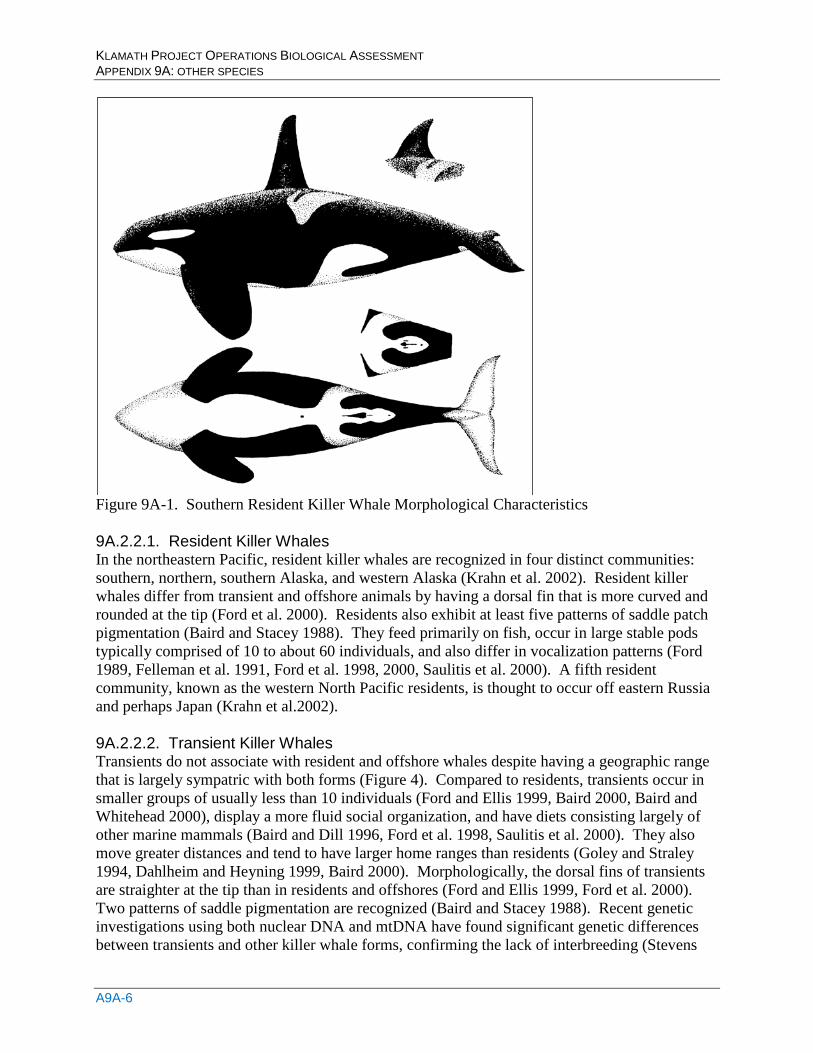
KLAMATH PROJECT OPERATIONS BIOLOGICAL ASSESSMENT APPENDIX 9A: OTHER SPECIES
A9A-6
Figure 9A-1. Southern Resident Killer Whale Morphological Characteristics 9A.2.2.1. Resident Killer Whales In the northeastern Pacific, resident killer whales are recognized in four distinct communities: southern, northern, southern Alaska, and western Alaska (Krahn et al. 2002). Resident killer whales differ from transient and offshore animals by having a dorsal fin that is more curved and rounded at the tip (Ford et al. 2000). Residents also exhibit at least five patterns of saddle patch pigmentation (Baird and Stacey 1988). They feed primarily on fish, occur in large stable pods typically comprised of 10 to about 60 individuals, and also differ in vocalization patterns (Ford 1989, Felleman et al. 1991, Ford et al. 1998, 2000, Saulitis et al. 2000). A fifth resident community, known as the western North Pacific residents, is thought to occur off eastern Russia and perhaps Japan (Krahn et al.2002). 9A.2.2.2. Transient Killer Whales Transients do not associate with resident and offshore whales despite having a geographic range that is largely sympatric with both forms (Figure 4). Compared to residents, transients occur in smaller groups of usually less than 10 individuals (Ford and Ellis 1999, Baird 2000, Baird and Whitehead 2000), display a more fluid social organization, and have diets consisting largely of other marine mammals (Baird and Dill 1996, Ford et al. 1998, Saulitis et al. 2000). They also move greater distances and tend to have larger home ranges than residents (Goley and Straley 1994, Dahlheim and Heyning 1999, Baird 2000). Morphologically, the dorsal fins of transients are straighter at the tip than in residents and offshores (Ford and Ellis 1999, Ford et al. 2000). Two patterns of saddle pigmentation are recognized (Baird and Stacey 1988). Recent genetic investigations using both nuclear DNA and mtDNA have found significant genetic differences between transients and other killer whale forms, confirming the lack of interbreeding (Stevens
KLAMATH PROJECT OPERATIONS BIOLOGICAL ASSESSMENT APPENDIX 9A: OTHER SPECIES
A9A-7
1989, Hoelzel and Dover 1991, Hoelzel et al. 1998, Barrett-Lennard 2000, Barrett-Lennard and Ellis 2001). These studies also indicate that up to three genetically distinct assemblages of transient killer whales exist in the northeastern Pacific. These are identified as 1) west coast transients, which occur from southern California to southeastern Alaska (Figure 4), 2) Gulf of Alaska transients, and 3) AT1 pod, which inhabits Prince William Sound and the Kenai Fjords in the northern Gulf of Alaska and is highly threatened with just nine whales remaining (Ford and Ellis 1999, Barrett-Lennard 2000, Barrett-Lennard and Ellis 2001). Genetic evidence suggests there is little or no interchange of members among these populations (Barrett-Lennard and Ellis 2001) 9A.2.2.3. Offshore Killer Whales Due to a scarcity of sightings, much less information is available for the offshore killer whale population, which was first identified in the late 1980’s (Ford et al. 1992, 1994, Walters et al 1992. Records are distributed from southern California to Alaska (Figure 4), including many from western Vancouver Island and the Queen Charlotte Islands (Ford and Ellis 1999, Krahn et al. 2002). Recent data from Alaska has extended the population’s range to the western Gulf of Alaska and eastern Aleutians (Wiley 2004.). Offshore killer whales usually occur 15 km or more offshore, but also visit coastal waters and occasionally enter protected inshore waters. Sightings have been made up to 500 km off the Washington coast (Krahn et al. 2002). Animals typically congregate in groups of 20-75 animals and are presumed to feed primarily on fish. Intermixing with residents and transients has not been observed. Genetic analyses indicate that offshore killer whales are reproductively isolated from other forms, but are more closely related to the southern residents (Hoelzel et al 1998, Barrett-Lennard and Ellis 2001). Offshores are thought to be slightly smaller in body size than residents and transients, and have dorsal fins and saddle patches resembling those of residents (Walters et al. 1992, Ford et al. 2000). 9A.2.3. Legal Status The southern resident killer whale DPS was listed as endangered under the ESA on November 18, 2005 (NMFS 2005b). NMFS (2008b) subsequently published a recovery plan for southern resident killer whales in 2008. The killer whale was also listed as an endangered state of Washington species in June 2004. NMFS determined that the southern resident stock was below its optimum sustainable population and designated it as depleted under the Marine Mammal Protection Act (MMPA) in May 2003 (68 FR 31980) and a Proposed Conservation Plan was announced in 2005 (70 FR 57565). The National Marine Fisheries Service (NMFS 2006b) designated critical habitat for the southern resident DPS on November 29, 2006. The following physical or biological critical habitat features are identified as essential to this species conservation: (1) water quality to support growth and development; (2) prey species of sufficient quantity, quality, and availability to support individual growth, reproduction, and development, as well as overall population growth; and (3) passage conditions to allow for migration, resting, and foraging. NMFS (2006b) identified three “specific areas” within the geographical area occupied by the species, which contain these important physical or biological features: (1) the Summer Core Area in Haro Strait
KLAMATH PROJECT OPERATIONS BIOLOGICAL ASSESSMENT APPENDIX 9A: OTHER SPECIES
A9A-8
and waters around the San Juan Islands; (2) Puget Sound; and (3) the Strait of Juan de Fuca. These critical habitat areas comprise approximately 2,560 square miles of marine habitat within the area occupied by southern Resident DPS killer whales in Washington. 9A.2.4 . Life History Social Organization: Killer whales are highly social animals that occur primarily in groups or pods of up to 40-50 animals (Dahlheim and Heyning 1999, Baird 2000). Mean pod size varies among populations, but often ranges from 2 to 15 animals (Kasuya 1971, Condy et al. 1978, Mikhalev et al. 1981, Braham and Dahlheim 1982, Dahlheim et al. 1982, Baird and Dill 1996). Larger aggregations of up to several hundred individuals occasionally form, but are usually considered temporary groupings of smaller social units that probably congregate near seasonal concentrations of prey, for social interaction, or breeding (Dahlheim and Heyning 1999, Baird 2000, Ford et al. 2000). Single whales, usually adult males, also occur in many populations (Norris and Prescott 1961, Hoelzel 1993, Baird 1994). Differences in spatial distribution, abundance, and behavior of food resources probably account for much of the variation in group size among killer whale populations. For example, sympatric populations of resident and transient whales in Washington and British Columbia vary substantially in average pod size. Transients forage in small groups on wary and patchily distributed marine mammals and are presumably able to maximize their per capita energy intake through reduced competition over food (Baird and Dill 1996, Ford and Ellis 1999, Baird and Whitehead 2000). In contrast, the larger groups of resident whales may be better able to detect schools of fish, enabling individual members to increase food consumption (Ford et al. 2000). The age and sex structure of killer whale social groups has been reported for populations at several locations. Olesiuk et al. (1990a) reported that pods in Washington and British Columbia were comprised of 19 percent adult males, 31 percent adult females, and 50 percent immature whales of either sex. In Alaska, 24 percent of the animals in pods were adult males, 47 percent were either adult females or subadult males, and 29 percent were younger animals (Dahlheim 1997, Dahlheim et al. 1997). For southern oceans, Miyazaki (1989) found that 16 percent of populations were adult males, 8 percent were adult females with calves, and 76 percent were immatures and adult females without calves. At Marion Island in the southern Indian Ocean, 29 percent of the population were adult males, 21 percent were adult females, 8 percent were calves, 25 percent were subadults, and 17 percent unidentified (Condy et al. 1978). Some of the most detailed studies of social structure in killer whales have been made in British Columbia, Washington, and Alaska during the past few decades, with much information available on group size, structure, and stability, and vocal traits (Ford 1989, 1991, Bigg et al. 1990, Matkin et al. 1999b, Ford et al. 2000, Yurk et al. 2002). Social organization in this region is based on maternal kinship and may be characteristic of killer whale populations throughout the world (Ford 2002). Vocalizations: Vocal communication is particularly advanced in killer whales and is an essential element of the species’ complex social structure. Like all dolphins, killer whales produce numerous types of vocalizations that are useful in navigation, communication, and foraging
KLAMATH PROJECT OPERATIONS BIOLOGICAL ASSESSMENT APPENDIX 9A: OTHER SPECIES
A9A-9
(Dahlheim and Awbrey 1982, Ford 1989, Barrett-Lennard et al.1996, Ford et al. 2000). Sounds are made by air forced through structures in the nasal passage and are enhanced and directed forward by a fatty enlargement near the top of the head, known as the melon. Most calls consist of both low- and high frequency components (Bain and Dahlheim 1994). The low-frequency component is relatively omnidirectional, with most energy directed forward and to the sides (Schevill and Watkins 1966). Diving and Swimming Behavior: Respiration rates of killer whales vary with activity level (Ford 1989). Dive cycles in transient whales average 5-8 minutes in total length and usually consist of three to five short dives lasting 10-35 seconds each followed by a longer dive averaging 4-7 minutes (range = 1-17 minutes) (Erickson 1978, Morton 1990, Ford and Ellis 1999). Surface blows following each of the short dives in a cycle last 3-4 seconds. Dive cycles in resident whales follow a similar pattern, but have long dives that are usually much briefer than in transients, averaging about 3 minutes and rarely exceeding 5 minutes (Morton 1990, Ford and Ellis 1999). Southern residents spend 95 percent of their time underwater, nearly all of which is between the surface and a depth of 30 m (Baird et al. 1998, 2003, Baird 2000). Preliminary information March 2004 14 Washington Department of Fish and Wildlife indicates that up to two dives per hour are made below 30 m. However, these represent fewer than 1 percent of all dives and occupy less than 2.5 percent of an animal’s total dive time. In the vicinity of the San Juan Islands, maximum dive depths averaged 141 m per animal among seven individuals tagged with time-depth recorders in July 2002 (Baird et al. 2003). One juvenile whale twice exceeded 228 m, causing Baird et al. (2003) to speculate that members of this population are probably capable of diving to 350 m, which is the approximate maximum bottom depth of the core inland waters of their summer range. The deepest dive reported for a killer whale is 260 m by a trained animal (Bowers and Henderson 1972). Killer whales normally swim at speeds of 5-10 km per hour, but can attain maximum speeds of 40 km per hour (Lang 1966, Erickson 1978, Kruse 1991, Williams et al. 2002a). Diving animals reach a velocity of 22 km per hour, or 6 m per second, during descents and ascents. Bursts in speed during dives commonly occur when prey are chased (Baird et al. 2003) Dispersal/Movements: Killer whale movements are generally thought to be far ranging, but detailed information on year round travel patterns is lacking for virtually all populations (Wiley 2004). Many killer whale populations appear to inhabit relatively well-defined seasonal home ranges linked to locations of favored prey, especially during periods of high prey abundance or vulnerability, such as fish spawning and seal pupping seasons (Jefferson et al. 1991, Reeves et al. 2002). Killer whale occurrence has been tied to migrating rorqual whales off eastern Canada (Sergeant and Fisher 1957), minke whale presence in southern oceans (Mikhalev et al. 1981, Pitman and Ensor 2003), sea lion and elephant seal pupping sites in the southwest Indian Ocean, Argentina, and North Pacific (Tomilin 1957, Norris and Prescott 1961, Condy et al. 1978, Lopez and Lopez 1985, Hoelzel 1991, Baird and Dill 1995), migrating herring (Clupea harengus) and other fish in the northeastern Atlantic (Jonsgård and Lyshoel 1970, Bloch and Lockyer 1988, Christensen 1988, Evans 1988, Similä et al. 1996), and returning salmon in the northeastern Pacific (Balcomb et al. 1980, Heimlich-Boran 1986a, 1988, Felleman et al. 1991, Nichol and
KLAMATH PROJECT OPERATIONS BIOLOGICAL ASSESSMENT APPENDIX 9A: OTHER SPECIES
A9A-10
Shackleton 1996). Defended territories have not been observed around these or other food sources (Dahlheim and Heyning 1999, Baird 2000). Annual north-south migrations has not been clearly documented for any killer whale population (Baird 2001), although such movements are suspected among some animals visiting the Antarctic (Mikhalev et al. 1981, Visser 1999a, Pitman and Ensor 2003). Regional movement patterns are probably best known for populations in the northeastern Pacific and may be illustrative of movements occurring in other parts of the world. Both resident and transient killer whales have been recorded year-round in Washington, British Columbia, and Alaska (Heimlich-Boran 1988, Baird and Dill 1995, Olson 1998, Baird 2001). Many pods inhabit relatively small core areas for periods of a few weeks or months, but travel extensively at other times. Known ranges of some individual whales or pods extend from central California to the Queen Charlotte Islands off northern British Columbia (a distance of about 2,200 km) for southern residents, from southern Vancouver Island to southeastern Alaska (about 1,200 km) for northern residents, from southeastern Alaska to Kodiak Island (about 1,450 km) for southern Alaska residents, and from central California to southeastern Alaska (about 2,660 km) for transients (Goley and Straley 1994; Dahlheim and Heyning 1999; Krahn et al. 2002; J. K. B. Ford and G. M. Ellis, unpubl. data). Both types of whales can swim up to 160 km per day (Erickson 1978, Baird 2000), allowing rapid movements between areas. For example, members of K and L pods once traveled a straight-line distance of about 940 km from the northern Queen Charlotte Islands to Victoria, Vancouver Island, in seven days (J. K. B. Ford and G. M. Ellis, unpubl. data). Other resident pods in Alaska have journeyed 740 km in six days and made a 1,900- km round trip during a 53-day period (Matkin et al. 1997). Transients are believed to travel greater distances and have larger ranges than residents (Goley and Straley 1994, Dahlheim and Heyning 1999, Baird 2000), as reflected by maximum home range estimates of 140,000 km2 for transients and 90,000 km2 for residents suggested by Baird (2000). A linear distance of 2,660 km covered by three transients from Glacier Bay, Alaska, to Monterey Bay, California (Goley and Straley 1994), is the longest recorded movement by the species. Reproduction: Killer whales are believed to mate in the North Pacific from May to October (Nishiwaki 1972, Olesiuk et al. 1990, Matkin et al. 1997). However, small numbers of conceptions apparently happen year-round, as evidenced by births of calves in all months. Gestation periods in captive killer whales average about 17 months (Asper et al. 1988, Duffield et al. 1995). Mean interval between viable calves is four years (Bain 1990). Newborns measure 2.2 to 2.7 m long and weigh about 200 kg (Nishiwaki and Handa 1958, Olesiuk et al. 1990, Clark et al. 2000, Ford 2002). Calves remain close to their mothers during their first year of life, often swimming slightly behind and to the side of the mother’s dorsal fin. Weaning age remains unknown, but nursing probably ends at 1 to 2 years of age (Kastelein et al. 2003). Mothers and offspring maintain highly stable social bonds throughout their lives and this natal relationship is the basis for the matrilineal social structure (Bigg et al. 1990, Baird 2000, Ford et al. 2000). 9A.2.5. Life Cycle Needs Killer whales frequent a variety of marine habitats with adequate prey resources and do not appear to be constrained by water depth, temperature, or salinity (Baird 2000). Although the
KLAMATH PROJECT OPERATIONS BIOLOGICAL ASSESSMENT APPENDIX 9A: OTHER SPECIES
A9A-11
species occurs widely as a pelagic inhabitant of open ocean, many populations spend large amounts of time in shallower coastal and inland marine waters, foraging even in inter-tidal areas in just a few meters of water. Killer whales tolerate a range of water temperatures, occurring from warm tropical seas to polar regions with ice floes and near freezing waters. Brackish waters and rivers are also occasionally entered (Scheffer and Slipp 1948, Tomilin 1957). Individual knowledge of productive feeding areas and other special habitats (e.g., beach rubbing sites in the Johnstone Strait) is probably an important determinant in the selection of locations visited and is likely a learned tradition passed from one generation to the next (Ford et al. 1998). Resident and transient killer whales exhibit somewhat different patterns of habitat use while in protected inland waters, where most observations are made (Heimlich-Boran 1988, Morton 1990, Felleman et al. 1991, Baird and Dill 1995). Residents generally spend more time in deeper water and only occasionally enter water less than 5 m deep (Heimlich-Boran 1988, Baird 2000, 2001). Distribution is strongly associated with areas of greater salmon abundance (Heimlich-Boran 1986a, 1988, Felleman et al. 1991, Nichol and Shackleton 1996), but research to date has yielded conflicting information on preferred foraging habitats. Several studies have reported that southern residents feed heavily in areas characterized by high-relief underwater topography, such as subsurface canyons, seamounts, ridges, and steep slopes (Heimlich-Boran 1988, Felleman et al. 1991). Such features may limit fish movements, thereby resulting in greater prey availability, and be used by the whales as underwater barriers to assist in herding fish (Heimlich-Boran 1988). As top-level predators, killer whales feed on a variety of marine organisms ranging from fish to squid to other marine mammal species. Chinook salmon reportedly comprise over 71 percent of the identified salmonids taken by killer whales (Ford and Ellis 2006). In particular, Ford and Ellis (2006) and Hanson et al. (2010) found that Chinook salmon comprise at least 84 percent of the diet of southern Resident killer whales (southern Residents) while the whales are in the Puget Sound/Juan de Fuca area. Southern resident killer whale survival and fecundity are correlated with Chinook salmon abundance, further indicating a Chinook salmon dietary preference (Ward et al. 2009, Ford et al. 2009). Ford and Ellis (2006) indicated that coastal killer whale populations also consume other salmonids in smaller proportions, including chum (O. keta, 22 percent of the diet) pink (O. gorbuscha, 3 percent), coho (O. kisutch, 2 percent), and sockeye (O. nerka, less than 1 percent) salmon, and steelhead (O. mykiss, less than 1 percent). Chemical analyses of killer whale fatty acids and contaminant ratios are also consistent with a salmon diet in killer whales (OCAP BA, 2008). The primary prey at greater depths may be Chinook salmon, which swim at depths averaging 25-80 m and extending down to 300-400 m (Candy and Quinn 1999). Other salmonids mostly inhabit the upper 30 m of the water column (Quinn and terHart 1987, Quinn et al. 1989, Ruggerone et al. 1990). As discussed in the coho salmon effects analysis, the Proposed Action's effects on the hydrology of the Klamath River are concentrated in the reaches immediately downstream of Iron Gate Dam (IGD), with those effects decreasing as the distance from IGD increases. Unlike coho salmon, Chinook salmon primarily spawn within the main stem of the Klamath River and in the channels of the larger tributaries of the Klamath River. That portion of the Chinook salmon population that spawns and rear in the main stem of the Klamath River immediately downstream of IGD is the population segment that has the greatest potential effect from implementing the Proposed
KLAMATH PROJECT OPERATIONS BIOLOGICAL ASSESSMENT APPENDIX 9A: OTHER SPECIES
A9A-12
Action. No estimates are available for the numbers of Chinook salmon spawning immediately downstream of IGD. However, natural spawning is known to occur throughout the basin and spawning is not concentrated in the reaches immediately downstream of IGD. The potential effect of implementing the Proposed Action to that fraction of the Chinook salmon population in the reaches closest to IGD are most likely small and not measureable. Thus, with the implementation of the Proposed Action, the potential reduction in the available prey for Orca in the marine environment are insignificant, or discountable. Hoelzel (1993) has reported no correlation between the feeding behavior of southern Resident killer whales and bottom topography, and found that most foraging took place over deep open water (41 percent of sightings), shallow slopes (32 percent), and deep slopes (19 percent). Ford et al. (1998) described residents as frequently foraging within 50-100 m of shore and using steep nearshore topography to corral fish. Both of these studies, plus those of Baird et al. (1998, 2003), have reported that most feeding and diving activity occurs in the upper 30 m of the water column, where most salmon are distributed (Stasko et al. 1976, Quinn and terHart 1987, Quinn et al. 1989, Ruggerone et al. 1990, Olson and Quinn 1993, Nichol and Shackleton 1996, Candy and Quinn 1999, Baird 2000). Additionally, Chinook salmon occupy nearshore habitats more so than other salmonids (Stasko et al. 1976, Quinn et al. 1989). Reasons for the discrepancies between studies are unclear, but may result from interpod variation and differences in study methodology (Nichol and Shackleton 1996, Baird 2001). Other behaviors, such as resting and socializing are performed in open water with varied bathymetry (Heimlich-Boran 1988, Felleman et al.1991). Habitat use patterns are poorly understood for southern resident pods visiting the outer coast. 9A.2.6. Distribution The southern Resident DPS killer whales consist of three pods, identified as J, K, and L pods. All three pods reside for part of the year in the inland waterways of Washington State and British Columbia (Strait of Georgia, Strait of Juan de Fuca, and Puget Sound), principally during the late spring, summer, and fall (Heimlich-Boran 1988, Felleman et al. 1991, Olson 1998, Osborne 1999, Ford et al. 2000, Krahn et al. 2002). Pods visit coastal sites off Washington and Vancouver Island (Ford et al. 2000), but travel as far south as central California and as far north as the Queen Charlotte Islands. Offshore movements and distribution are largely unknown for the southern Resident DPS killer whale. 9A.2.7. Species Current Condition The southern Resident killer whale population and its current status are shown from 1974 – 2007 in Table 6-1. The population has reportedly declined to essentially the same size that was estimated during the early 1960s, when it was considered likely depleted (Olesiuk et al. 1990). Since 1974, J and K pods have increased in sizes by 60 percent (mean of 1.9 percent per year) and 38 percent (mean of 1.2 percent per year), respectively. The largest pod, L pod, has grown 28.6 percent (mean of 0.9 percent per year) during this same period, but most recently experienced a 10-year decline from 1994 to 2003 that threatened to reduce the pod’s size below any previously recorded level. Data from 2002 to 2006 indicates that L pod’s decline may have finally ended; however, this slight upward population trend in recent years is not conclusive (NMFS 2008b).
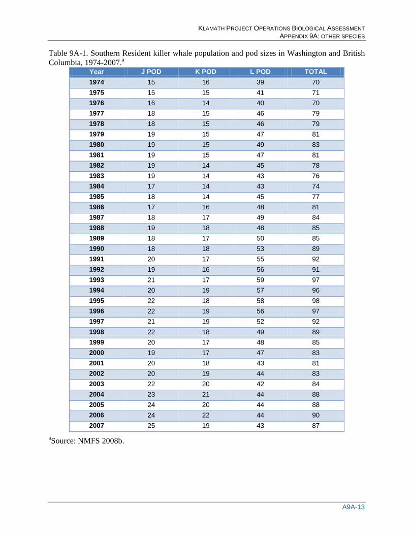
KLAMATH PROJECT OPERATIONS BIOLOGICAL ASSESSMENT APPENDIX 9A: OTHER SPECIES
A9A-13
Table 9A-1. Southern Resident killer whale population and pod sizes in Washington and British Columbia, 1974-2007.a
Year J POD K POD L POD TOTAL 1974 15 16 39 70 1975 15 15 41 71 1976 16 14 40 70 1977 18 15 46 79 1978 18 15 46 79 1979 19 15 47 81 1980 19 15 49 83 1981 19 15 47 81 1982 19 14 45 78 1983 19 14 43 76 1984 17 14 43 74 1985 18 14 45 77 1986 17 16 48 81 1987 18 17 49 84 1988 19 18 48 85 1989 18 17 50 85 1990 18 18 53 89 1991 20 17 55 92 1992 19 16 56 91 1993 21 17 59 97 1994 20 19 57 96 1995 22 18 58 98 1996 22 19 56 97 1997 21 19 52 92 1998 22 18 49 89 1999 20 17 48 85 2000 19 17 47 83 2001 20 18 43 81 2002 20 19 44 83 2003 22 20 42 84 2004 23 21 44 88 2005 24 20 44 88 2006 24 22 44 90 2007 25 19 43 87
aSource: NMFS 2008b.
KLAMATH PROJECT OPERATIONS BIOLOGICAL ASSESSMENT APPENDIX 9A: OTHER SPECIES
A9A-14
9A.3. Other Species 9A.3.1. Southern DPS Pacific Eulachon 9A.3.1.1. Species Description Eulachon Thaleichthys Pacificus (commonly called smelt, candlefish, or hooligan) are a small, anadromous fish from the eastern Pacific eulachon are a short-lived, high-fecundity, high-mortality forage fish, and tend to have extremely large population sizes. NMFS (2012c) describes the following distinguishing physical features: large canine teeth on the vomer (bone in the roof of the mouth) and 18 to 23 rays in the anal fin; sickle-shaped adipose fin; fins have well-developed breeding tubercles (raised tissue "bumps") in ripe males, but these are poorly developed or absent in females; adult coloration is brown to blue on the back and top of the head, lighter to silvery white on the sides, and white on the ventral surface; speckling is fine, sparse, and restricted to the back. Eulachon feed on plankton only while at sea. 9A.3.1.2. Legal Status NMFS listed the southern DPS Pacfic eulachon as threatened under the ESA on March 18, 2010 (75 FR 13012). This DPS encompasses all populations within the states of Washington, Oregon, and California and extends from the Skeena River in British Columbia (inclusive) south to the Mad River in Northern California (inclusive). The DPS is divided into four sub-areas: Klamath River, Columbia River, Fraser River, and British Columbia coastal rivers south of the Nass River. NMFS proposed to designate approximately 470.2 km (291.1 mi) of riverine and estuary habitat in California, Oregon, and Washington within the geographical area occupied by the southern DPS Pacific eulachon as critical habitat (NMFS 2010d). NMFS in 2011 designated final critical habitat for eulachon based upon areas which contain one or more physical or biological features essential to the conservation of the species that may require special management considerations or protection (NMFS 2011b).. NMFS (2011b) has designated final critical habitat for 10.7 miles of the Klamath River from the mouth upstream to the confluence with Omogar Creek.. 9A.3.1.3. Life History Eulachon typically spend three to five years in saltwater before returning to fresh water to spawn. Eulachon generally spawn in rivers that are either glacier or snow packed fed and that experience spring freshets. Spawning grounds are typically in the lower reaches of larger rivers (Hay and McCarter 2000). Spawning typically occurs at night. Spawning occurs at between 0 to 10°C throughout the range of the species, and is largely limited to the part of the river that is tidally influenced (Lewis et al. 2002). Spawning cues and entry into rivers appear to be related to water temperature and the occurrence of high tides (Ricker et al. 1954, Smith and Saalfeld 1955, Spangler 2002) in January, February, and March in the northern part of the DPS, and later in the spring in the southern parts of the DPS. Most eulachon adults die after spawning. Eulachon broadcast their eggs which are fertilized in the water column, sink, and adhere to the river bottom typically in areas of gravel and coarse sand. It has been argued that because freshets rapidly move eulachon eggs and larvae to estuaries, it is likely that eulachon imprint and home to an estuary into which several rivers
KLAMATH PROJECT OPERATIONS BIOLOGICAL ASSESSMENT APPENDIX 9A: OTHER SPECIES
A9A-15
drain rather than to individual spawning rivers (Hay and McCarter 2000). Eulachon eggs hatch in 20 to 40 days. Newly hatched young, transparent and 4 to 7 mm in length, are carried to the sea with the current (Hay and McCarter 2000). Juvenile eulachon enter the ocean once they move from shallow nearshore areas to deeper areas over the continental shelf. Larvae and young juveniles become widely distributed in coastal waters, where they are typically found near the ocean bottom in waters 20 to150 m deep (66 to 292 ft) (Hay and McCarter 2000) and sometimes as deep as 182 m (597 ft) (Barraclough 1964). There is currently little information available about eulachon movements in nearshore marine areas and the open ocean. However, eulachon occur as bycatch in the pink shrimp fishery (Hay et al. 1999, Olsen et al. 2000, NWFSC 2008, Hannah and Jones 2009), which indicates that the distribution of these organisms overlaps in the ocean. Adult Pacific eulachon have been recorded from several locations on the Washington and Oregon coasts, and were previously common in Oregon’s Umpqua River, and the Klamath River in northern California (Hay and McCarter 2000, Willson et al. 2006, NMFS 2010b). 9A.3.1.4. Species Current Condition There are few direct estimates of abundance available for eulachon, and there is an absence of monitoring programs in the United States. Most population data comes from fishery catch and landing records, which when combined with anecdotal information, indicate eulachon historically were present in large annual runs and that significant declines in abundance have occurred (Reclamation 2011). The Columbia River, estimated to have historically represented fully half of the taxon’s abundance, experienced a sudden decline in its commercial eulachon fishery landings in 1993–1994 (Washington Department of Fish and Wildlife [WDFW] and ODFW 2001, JCRMS 2007). Similar declines in abundance have occurred in the Fraser River and other coastal British Columbia rivers (Hay and McCarter 2000, Moody 2008). In the Klamath River and the Umpqua River, eulachon were once abundant, but have declined to the point where detecting them has become difficult (NMFS 2010b). There has been no long-term monitoring program targeting eulachon in California, making estimates of historical abundance and abundance trends difficult to generate (Gustafson et al. 2008).