Embed Size (px)
Citation preview
APPLICATION OF POWER TO GAS
(P2G) SYSTEMS IN DANISH
ELECTRIC DISTRIBUTION NETWORKS
MSc Thesis – Department of Energy Technology
Spring semester 2015
Aina Romaní Dalmau and David Martínez Pérez

Title: Application of Power to Gas (P2G) Systems in Danish Electric DistributionNetworks
Semester: 3rd and 4th
Project period: Master’s ThesisECTS: 01/09/14 - 27/05/15Supervisors: Jayakrishnan Radhakrishna Pillai and Iker Diaz de Zerio MendazaProject group: EPSH4-933
David Martínez Pérez
Aina Romaní Dalmau
Copies: 3Pages, total: 152Appendices: A, B, C & DSupplements: CD
SYNOPSIS:
According to the latest energy policy, wind power shareis expected to increase in order to allow Denmark tobecome fossil fuel free by 2050. This high wind powerpenetration is expected to introduce several challengesinto the power system, such as large power imbalancesor voltage rise. In order to tackle these issues, energystorage systems represent a possible solution for ab-sorbing the wind power excess. Concerning the Danishcase, the state-of-the art district heating and gas net-works comprise perfect energy storage solutions. In thiscontext, Power to Gas turns out to be an interestingoption in order to inject the electricity excess into thegas network. This system is based on transformationof electricity to hydrogen by use of electrolyzers. Theproduced hydrogen can be directly injected into the gasgrid or transformed into natural gas in an intermediatestep. The present MSc Thesis focuses on testing thecapability of an alkaline electrolyzer to deliver voltageregulation and energy management services to a typicalDanish distribution grid with a high wind power pene-tration. The electrolyzer is integrated with the typicalvoltage regulation assets present in a distribution grid.One of the main targets of this project is to find a con-trol strategy where the mentioned voltage regulationand energy management services coexist in a marketenvironment.
By signing this document, each member of the group confirms that all participated in theproject work and thereby all members are collectively liable for the content of the report.Furthermore, all group members confirm that the report does not include plagiarism.


Application of Power to Gas (P2G) Systems in Danish Electric Distribution Networks iii
PrefaceThis report has been written by group EPSH4-933 on the 3rd and 4th semester at the Departmentof Energy Technology at Aalborg University in the period from the 2nd of September 2014 untilthe 27th of May 2015. The purpose of this project is to analyze the technical impact of integratinga P2G system in a typical Danish medium voltage grid.
We as a group would like to thank our supervisors Iker Diaz de Zerio Mendaza and JayakrishnanRadhakrishna Pillai for their guidance, patience and support throughout the development of thisproject. Additionally, we would like to express our gratitude to Carolina Carmo (INSERO Energy)and Jesper Bruun (Energinet.dk) for providing us with valuable information and data.
In this project the software DIgSILENT PowerFactory has been used to simulate an electricaldistribution grid and its elements. Additionally, the software Matlab has been used to analyzedata and execute calculations. The present report has been written using LATEX.
Reader’s Guide The used information in the present work has been found in literature, webpages and reports. The sources are cited through the report and can be found in the Bibliography.The method for referring to these sources is the IEEE citation style, which refers to the sourceswith a [number] by order of appearance. All references can be found on the CD, except the usedbooks and websites. Additionally, tables, figures and equations are labeled with the number ofthe chapter.
The CD attached in the report contains the PDF of the project document, the relevant Power-Factory and Matlab files and the references that were available in PDF format.

Application of Power to Gas (P2G) Systems in Danish Electric Distribution Networks v
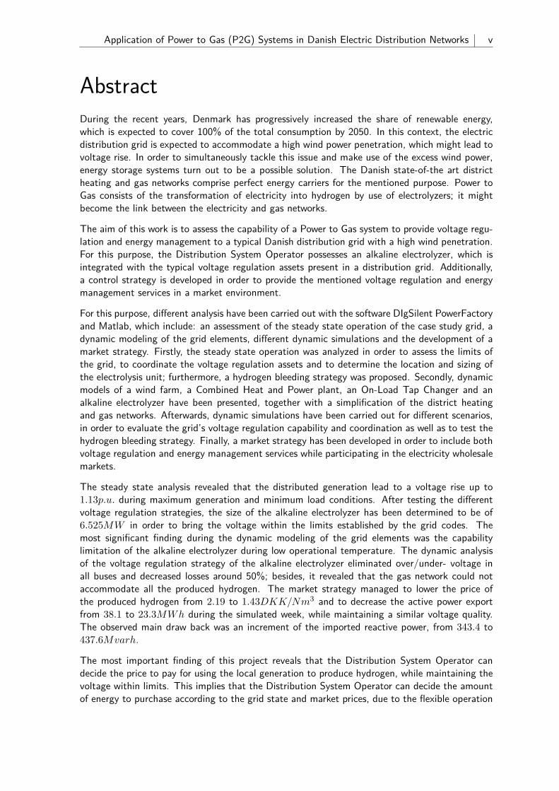
AbstractDuring the recent years, Denmark has progressively increased the share of renewable energy,which is expected to cover 100% of the total consumption by 2050. In this context, the electricdistribution grid is expected to accommodate a high wind power penetration, which might lead tovoltage rise. In order to simultaneously tackle this issue and make use of the excess wind power,energy storage systems turn out to be a possible solution. The Danish state-of-the art districtheating and gas networks comprise perfect energy carriers for the mentioned purpose. Power toGas consists of the transformation of electricity into hydrogen by use of electrolyzers; it mightbecome the link between the electricity and gas networks.
The aim of this work is to assess the capability of a Power to Gas system to provide voltage regu-lation and energy management to a typical Danish distribution grid with a high wind penetration.For this purpose, the Distribution System Operator possesses an alkaline electrolyzer, which isintegrated with the typical voltage regulation assets present in a distribution grid. Additionally,a control strategy is developed in order to provide the mentioned voltage regulation and energymanagement services in a market environment.
For this purpose, different analysis have been carried out with the software DIgSilent PowerFactoryand Matlab, which include: an assessment of the steady state operation of the case study grid, adynamic modeling of the grid elements, different dynamic simulations and the development of amarket strategy. Firstly, the steady state operation was analyzed in order to assess the limits ofthe grid, to coordinate the voltage regulation assets and to determine the location and sizing ofthe electrolysis unit; furthermore, a hydrogen bleeding strategy was proposed. Secondly, dynamicmodels of a wind farm, a Combined Heat and Power plant, an On-Load Tap Changer and analkaline electrolyzer have been presented, together with a simplification of the district heatingand gas networks. Afterwards, dynamic simulations have been carried out for different scenarios,in order to evaluate the grid’s voltage regulation capability and coordination as well as to test thehydrogen bleeding strategy. Finally, a market strategy has been developed in order to include bothvoltage regulation and energy management services while participating in the electricity wholesalemarkets.
The steady state analysis revealed that the distributed generation lead to a voltage rise up to1.13p.u. during maximum generation and minimum load conditions. After testing the differentvoltage regulation strategies, the size of the alkaline electrolyzer has been determined to be of6.525MW in order to bring the voltage within the limits established by the grid codes. Themost significant finding during the dynamic modeling of the grid elements was the capabilitylimitation of the alkaline electrolyzer during low operational temperature. The dynamic analysisof the voltage regulation strategy of the alkaline electrolyzer eliminated over/under- voltage inall buses and decreased losses around 50%; besides, it revealed that the gas network could notaccommodate all the produced hydrogen. The market strategy managed to lower the price ofthe produced hydrogen from 2.19 to 1.43DKK/Nm3 and to decrease the active power exportfrom 38.1 to 23.3MWh during the simulated week, while maintaining a similar voltage quality.The observed main draw back was an increment of the imported reactive power, from 343.4 to437.6Mvarh.
The most important finding of this project reveals that the Distribution System Operator candecide the price to pay for using the local generation to produce hydrogen, while maintaining thevoltage within limits. This implies that the Distribution System Operator can decide the amountof energy to purchase according to the grid state and market prices, due to the flexible operation

vi Application of Power to Gas (P2G) Systems in Danish Electric Distribution Networks
of the different voltage regulation assets. However, a cost/benefit analysis must be done in orderto implement Power to Gas technology in a profitable way. With a reduction of the currentlyexpensive costs of the technology, its application could become economically feasible and couldopen the possibility to new business opportunities.
List of Figures
1.1 Wind power and load profile for the present and for 2050 in Denmark [2] . . . . . . 11.2 Possible solutions for the integration of Renewable Energy Systems (RES) [4] . . . . 21.3 Technical comparison for both power and capacity of the different ESS [4] . . . . . . 31.4 Economical comparison of the capacity of the different ESS [4] . . . . . . . . . . . . 3
2.1 Existing Danish Transmission System in 2014 [13] . . . . . . . . . . . . . . . . . . . 92.2 Single-line diagram of the different grid topologies . . . . . . . . . . . . . . . . . . . 102.3 Markets for flexibility in the upcoming power system [20] . . . . . . . . . . . . . . . 112.4 Diagram representing the integration of electricity, gas and district heating sectors [2] 122.5 Basic Brayton cycle diagram [23] . . . . . . . . . . . . . . . . . . . . . . . . . . . . 142.6 The Danish transmission gas network in 2014 [30] . . . . . . . . . . . . . . . . . . . 15
3.1 Single-line diagram of the benchmark MV grid [48] . . . . . . . . . . . . . . . . . . 203.2 Industrial and residential load profiles during a winter week . . . . . . . . . . . . . . 203.3 Industrial and residential load profiles during a summer week . . . . . . . . . . . . . 203.4 Sketch of the proposed hydrogen injection in the study case grid . . . . . . . . . . . 223.5 Load flow of the grid in DIgSILENT at maximum generation & without OLTC . . . 243.6 Load flow of the grid in DIgSILENT at minimum generation & without OLTC . . . . 253.7 Load flow of the grid in DIgSILENT at maximum generation & OLTC . . . . . . . . 273.8 Load flow of the grid in DIgSILENT at no generation & OLTC . . . . . . . . . . . . 283.9 Reactive power requirements for wind power plants with a power output range between
1.5 and 25 MW [63] . . . . . . . . . . . . . . . . . . . . . . . . . . . . . . . . . . . 293.10 PQ capability curve of the CHP units’ synchronous generator and requested operation
points . . . . . . . . . . . . . . . . . . . . . . . . . . . . . . . . . . . . . . . . . . 303.11 Vector diagram of the DG voltage and its injected current, according to the intelligent
power factor control [67] . . . . . . . . . . . . . . . . . . . . . . . . . . . . . . . . 313.12 Single-line diagram of the grid including alkaline electrolyzer load . . . . . . . . . . 333.13 Voltage - power droop control of the AE . . . . . . . . . . . . . . . . . . . . . . . . 343.14 Coordination of the OLTC, power factor controller and the AE . . . . . . . . . . . . 343.15 Load flow of the grid in DIgSILENT at maximum generation, OLTC and 6.525 MW
of electrolyzers . . . . . . . . . . . . . . . . . . . . . . . . . . . . . . . . . . . . . . 353.16 Load flow of the grid in DIgSILENT at no generation, OLTC and 6.525 MW of
electrolyzers . . . . . . . . . . . . . . . . . . . . . . . . . . . . . . . . . . . . . . . 363.17 Voltage results of the performed load flows during Case 1 . . . . . . . . . . . . . . . 383.18 Voltage results of the performed load flows during Case 2 . . . . . . . . . . . . . . . 383.19 Line and transformer loading results of the performed load flows during (a) Case 1
and (b) Case 2 . . . . . . . . . . . . . . . . . . . . . . . . . . . . . . . . . . . . . 383.20 Active and reactive power import of Feeder 1 during (a) Case 1 and (b) Case 2 . . . 393.21 Total line loss results of the performed load flows during (a) Case 1 and (b) Case 2 . 39
4.1 Wind farm active power calculation from wind speed measurement . . . . . . . . . . 42
vii
viii Application of Power to Gas (P2G) Systems in Danish Electric Distribution Networks
4.2 Comparison between the estimated wind power curve (left) and the provided by themanufacturer (right) . . . . . . . . . . . . . . . . . . . . . . . . . . . . . . . . . . 43
4.3 Composite model for the wind farm power output . . . . . . . . . . . . . . . . . . . 444.4 Wind active power output during the winter week [72] . . . . . . . . . . . . . . . . 444.5 Wind active power output during the summer week [72] . . . . . . . . . . . . . . . 444.6 Composite model for the wind farm reactive power control of the wind farm . . . . . 454.7 Block diagram of the reactive power control of the wind farm . . . . . . . . . . . . 454.8 DIgSILENT PowerFactory composite model of the CHP plant . . . . . . . . . . . . 464.9 Modified composite model for the CHP units . . . . . . . . . . . . . . . . . . . . . 474.10 Active and reactive power output from a CHP unit . . . . . . . . . . . . . . . . . . 474.11 Composite model of the CHP plant reactive power control . . . . . . . . . . . . . . 474.12 Block diagram of the Q control block of the CHP . . . . . . . . . . . . . . . . . . . 474.13 Model of the heat storage block of the CHP . . . . . . . . . . . . . . . . . . . . . . 484.14 Skagen’s CHP units output during the winter week . . . . . . . . . . . . . . . . . . 494.15 Skagen’s tank’s state of energy during the winter week . . . . . . . . . . . . . . . . 494.16 Heat demand, generated heat from boilers and generated heat from one CHP unit in
the winter week . . . . . . . . . . . . . . . . . . . . . . . . . . . . . . . . . . . . . 494.17 State of energy of the CHP’s heat storage . . . . . . . . . . . . . . . . . . . . . . . 494.18 Skagen’s CHP units output during the summer week . . . . . . . . . . . . . . . . . 504.19 Skagen’s tank’s state of energy during the summer week . . . . . . . . . . . . . . . 504.20 Heat demand, generated heat from boilers and generated heat from one CHP unit . 504.21 State of energy of the CHP’s heat storage . . . . . . . . . . . . . . . . . . . . . . . 504.22 Gas consumption of the CHP in [Nm3/h], during the winter week . . . . . . . . . . 514.23 Gas consumption of the CHP in [Nm3/h], during the summer week . . . . . . . . . 514.24 Composite frame of the OLTC controller . . . . . . . . . . . . . . . . . . . . . . . . 514.25 Composite frame of the Load Drop Compensation . . . . . . . . . . . . . . . . . . . 524.26 Voltage in bus 9 . . . . . . . . . . . . . . . . . . . . . . . . . . . . . . . . . . . . . 534.27 Current tap position of TRF1 . . . . . . . . . . . . . . . . . . . . . . . . . . . . . . 534.28 Composite frame of the control, modeling and grid implementation of the 15 elec-
trolyzer modules . . . . . . . . . . . . . . . . . . . . . . . . . . . . . . . . . . . . . 544.29 Block diagram of the active and reactive power control of the 15 electrolyzer modules 544.30 Composite frame of the alkaline electrolyzer module . . . . . . . . . . . . . . . . . . 554.31 Block diagram of the load control slot of the alkaline electrolyzer . . . . . . . . . . . 564.32 Block diagram of the alkaline electrolyzer . . . . . . . . . . . . . . . . . . . . . . . 564.33 U-I characteristic curves for different temperatures of the alkaline electrolyzer . . . . 574.34 Operating temperature [°C] of the 355kW alkaline electrolyzer . . . . . . . . . . . . 584.35 Active power set-points (red) and actual consumption (blue) [MW] of the 355kW
alkaline electrolyzer . . . . . . . . . . . . . . . . . . . . . . . . . . . . . . . . . . . 584.36 Reactive power set-points (red) and actual output (red) of the alkaline electrolyzer . 594.37 Active (blue) and reactive power (red) from the compressor . . . . . . . . . . . . . . 594.38 Composite frame of the hydrogen storage . . . . . . . . . . . . . . . . . . . . . . . 594.39 Wind farm active power output . . . . . . . . . . . . . . . . . . . . . . . . . . . . . 604.40 CHP unit 1 active power output . . . . . . . . . . . . . . . . . . . . . . . . . . . . 604.41 Electrolyzer’s active power consumption . . . . . . . . . . . . . . . . . . . . . . . . 60
5.1 Results of the grid in base case, during a winter week . . . . . . . . . . . . . . . . . 625.2 Results of the grid in base case, during day 1 of the winter week . . . . . . . . . . . 625.3 Results of the grid in base case, during a summer week . . . . . . . . . . . . . . . . 635.4 Results of the grid in base case, during day 1 of the summer week . . . . . . . . . . 635.5 Results of the grid with OLTC implementation, during a winter week . . . . . . . . . 655.6 Results of the grid with OLTC implementation, during day 1 of the winter week . . . 65
List of Figures ix
5.7 Results of the grid with OLTC implementation, during a summer week . . . . . . . . 665.8 Results of the grid with OLTC implementation, during day 1 of the summer week . . 675.9 Results of the grid with reactive power dispatch, during a winter week . . . . . . . . 685.10 Results of the grid with reactive power dispatch, during day 1 of the winter week . . 695.11 Results of the grid with reactive power dispatch, during a summer week . . . . . . . 705.12 Results of the grid with reactive power dispatch, during day 1 of the summer week . 715.13 Results of the grid with P2G implementation, during a winter week . . . . . . . . . 735.14 Results of the grid with P2G implementation, during day 1 of the winter week . . . . 745.15 Alkaline Electrolyzers parameters, during a winter week . . . . . . . . . . . . . . . . 755.16 Alkaline Electrolyzers parameters, during day 5 of the winter week . . . . . . . . . . 755.17 Hydrogen storage relevant variables, during a winter week . . . . . . . . . . . . . . 765.18 Results of the grid with P2G implementation, during a summer week . . . . . . . . . 775.19 Results of the grid with P2G implementation, during day 1 of the summer week . . . 785.20 Alkaline Electrolyzers parameters, during a summer week . . . . . . . . . . . . . . . 795.21 Alkaline Electrolyzers parameters, during day 5 of the summer week . . . . . . . . . 795.22 Hydrogen storage relevant variables, during a summer week . . . . . . . . . . . . . . 80
6.1 Basic scheme of the scheduling process . . . . . . . . . . . . . . . . . . . . . . . . 856.2 Basic scheme of the bidding process . . . . . . . . . . . . . . . . . . . . . . . . . . 856.3 Detailed scheme of the market strategy . . . . . . . . . . . . . . . . . . . . . . . . 866.4 Overall flowchart of the market strategy . . . . . . . . . . . . . . . . . . . . . . . . 876.5 Actual hourly wind power vs. hour and day ahead estimations . . . . . . . . . . . . 886.6 Flowchart of the voltage regulation algorithm . . . . . . . . . . . . . . . . . . . . . 906.7 Flowchart of the energy management algorithm . . . . . . . . . . . . . . . . . . . . 916.8 Flowchart of the maximum power algorithm . . . . . . . . . . . . . . . . . . . . . . 936.9 Typical structure of a fuzzy logic system [79] . . . . . . . . . . . . . . . . . . . . . 946.10 Membership functions for the market prices . . . . . . . . . . . . . . . . . . . . . . 956.11 Correlation between spot price and wind power generation in DK1 area during 2014 . 956.12 Bid in the spot market for hour 27, winter week . . . . . . . . . . . . . . . . . . . . 976.13 Voltage in bus 9 in the market case, winter week . . . . . . . . . . . . . . . . . . . 976.14 Active power export through TR1 in the market case, winter week . . . . . . . . . . 986.15 Alkaline electrolyzer’s active power consumption in the market case, winter week . . 986.16 Modified AE’s control composite frame for the market case . . . . . . . . . . . . . . 996.17 Modified AE’s set-point calculation block for the market case . . . . . . . . . . . . . 1006.18 Modified coordination of the voltage regulation assets for the market case . . . . . . 1016.19 Results of the grid implementing the market strategy, during the winter week . . . . 1026.20 Alkaline Electrolizer parameters, during the winter week . . . . . . . . . . . . . . . . 1036.21 Hydrogen storage relevant variables, during the winter week . . . . . . . . . . . . . 104
A.1 Forwarded bid from a Norwegian player [17] . . . . . . . . . . . . . . . . . . . . . . 114A.2 Aggregated curves and formation of spot price [16] . . . . . . . . . . . . . . . . . . 114A.3 Activated power and time of activation for primary, secondary and tertiary regulation
[80] . . . . . . . . . . . . . . . . . . . . . . . . . . . . . . . . . . . . . . . . . . . . 115
B.1 Wind speed measurement extrapolation to hub height [73] . . . . . . . . . . . . . . 119B.2 Block diagram of the GAST governor of the CHP [82] . . . . . . . . . . . . . . . . 120B.3 Block diagram of the excitation system of the CHP [82] . . . . . . . . . . . . . . . 121B.4 Block diagram of the power factor controller . . . . . . . . . . . . . . . . . . . . . . 122
C.1 Time sweep representation of the bus voltages using winter profile at Case 1 . . . . 123C.2 Time sweep representation of the bus voltages using winter profile at Case 2 . . . . 123C.3 Time sweep representation of the bus voltages using summer profile at Case 1 . . . . 123

x Application of Power to Gas (P2G) Systems in Danish Electric Distribution Networks
C.4 Time sweep representation of the bus voltages using summer profile at Case 2 . . . . 124

List of Tables
2.1 Amount of different CHP types and installed capacity in Denmark in 2013 [24] . . . 132.2 Characteristics of gas turbine generators [23] . . . . . . . . . . . . . . . . . . . . . 142.3 Comparation between the different electrolysis technologies [32] . . . . . . . . . . . 16
3.1 Summary of the rated generation and loads in the grid . . . . . . . . . . . . . . . . 193.2 Load type modeling approximations [50] . . . . . . . . . . . . . . . . . . . . . . . . 213.3 Data of the CHP plant of Skagen and calculated data of the case study CHP [54] [55] 223.4 Estimation of relevant parameters for calculating the natural gas consumption of the
CHP plant [23] [57] . . . . . . . . . . . . . . . . . . . . . . . . . . . . . . . . . . . 223.5 Comparison of critical voltages in Cases 1 and 2 with and without tap control . . . . 293.6 Comparison of critical voltages in Cases 1 and 2 with only tap control and with both
tap control and reactive power dispatch . . . . . . . . . . . . . . . . . . . . . . . . 323.7 Comparison of critical voltages in Cases 1 and 2 with reactive power dispatch and
with 6.525 MW of electrolyzers, both with tap control . . . . . . . . . . . . . . . . 37
4.1 Owners and available control for the DSO of different elements of the grid . . . . . 414.2 Relevant characteristics of the Vestas V80 2MW turbine [71] . . . . . . . . . . . . . 42
5.1 Total generation, load, external grid import and losses, during the winter week . . . 625.2 Total generation, load, external grid import and losses, during the summer week . . 645.3 Total generation, load, external grid import and losses, during the winter week . . . 665.4 Total generation, load, external grid import and losses, during the summer week . . 675.5 Total generation, load, external grid import and losses, during the winter week . . . 705.6 Total generation, load, external grid import and losses, during the summer week . . 725.7 Total generation, load, external grid import and losses, during the winter week . . . 765.8 Total generation, load, external grid import and losses, during the summer week . . 795.9 Voltage quality, grid losses, reactive power import and number of tap changes during
the analyzed cases . . . . . . . . . . . . . . . . . . . . . . . . . . . . . . . . . . . . 80
6.1 Fuzzy rules for the decision making . . . . . . . . . . . . . . . . . . . . . . . . . . . 956.2 Economical comparison between the market and the voltage regulation cases . . . . 986.3 Total generation, load, external grid import and losses comparison between the market
and voltage regulation cases, winter week . . . . . . . . . . . . . . . . . . . . . . . 1046.4 Economical comparison between the market and the voltage regulation cases . . . . 1056.5 Dynamic simulation results’ summary for both market and voltage regulation cases,
winter week . . . . . . . . . . . . . . . . . . . . . . . . . . . . . . . . . . . . . . . 105
B.1 Positive sequence parameters of the two different types of lines . . . . . . . . . . . . 117B.2 Line data . . . . . . . . . . . . . . . . . . . . . . . . . . . . . . . . . . . . . . . . . 117B.3 Transformer data [48], [82] . . . . . . . . . . . . . . . . . . . . . . . . . . . . . . . 118B.4 Rated power, power factor and profile type of the residential loads of the system . . 118
xi

xii Application of Power to Gas (P2G) Systems in Danish Electric Distribution Networks
B.5 Rated power and power factor of the industrial loads of the system . . . . . . . . . . 118B.6 Constant power and impedance coefficients of the loads of the grid . . . . . . . . . 119B.7 Gas turbine generator data . . . . . . . . . . . . . . . . . . . . . . . . . . . . . . . 120B.8 Gas turbine governor data . . . . . . . . . . . . . . . . . . . . . . . . . . . . . . . . 121B.9 Excitation system data . . . . . . . . . . . . . . . . . . . . . . . . . . . . . . . . . 121B.10 Estimated number of households in each bus . . . . . . . . . . . . . . . . . . . . . 122B.11 General parameters of the alkaline electrolyzer . . . . . . . . . . . . . . . . . . . . . 122
Nomenclature xiii
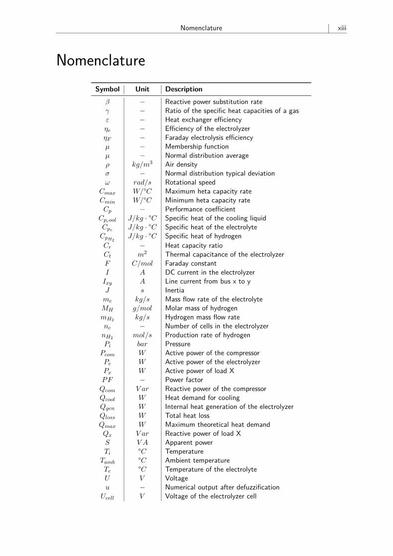
NomenclatureSymbol Unit Description
β − Reactive power substitution rateγ − Ratio of the specific heat capacities of a gasε − Heat exchanger efficiencyηe − Efficiency of the electrolyzerηF − Faraday electrolysis efficiencyµ − Membership functionµ − Normal distribution averageρ kg/m3 Air densityσ − Normal distribution typical deviationω rad/s Rotational speed
Cmax W/°C Maximum heta capacity rateCmin W/°C Minimum heta capacity rateCp − Performance coefficient
Cpcool J/kg · °C Specific heat of the cooling liquidCpe J/kg · °C Specific heat of the electrolyteCpH2
J/kg · °C Specific heat of hydrogenCr − Heat capacity ratioCt m2 Thermal capacitance of the electrolyzerF C/mol Faraday constantI A DC current in the electrolyzerIxy A Line current from bus x to yJ s Inertiame kg/s Mass flow rate of the electrolyteMH g/mol Molar mass of hydrogenmH2 kg/s Hydrogen mass flow ratenc − Number of cells in the electrolyzernH2 mol/s Production rate of hydrogenPi bar PressurePcom W Active power of the compressorPe W Active power of the electrolyzerPx W Active power of load XPF − Power factorQcom V ar Reactive power of the compressorQcool W Heat demand for coolingQgen W Internal heat generation of the electrolyzerQloss W Total heat lossQmax W Maximum theoretical heat demandQx V ar Reactive power of load XS V A Apparent powerTi °C TemperatureTamb °C Ambient temperatureTe °C Temperature of the electrolyteU V Voltageu − Numerical output after defuzzification
Ucell V Voltage of the electrolyzer cell

xiv Application of Power to Gas (P2G) Systems in Danish Electric Distribution Networks
Ue V Voltage of the electrolyzerUrev V Reversible voltageUth V Voltage threshold for the heat release processv m/s Wind speed
VDG V Voltage at the PCC of the DGV Nm3/h Volume flowVn V Nominal voltageVx V Voltage of bus XWi J/kg Energy rate of the heat exchangez − Number of electrons transferred in the reactionZxy Ω Impedance of the line from bus x to y
Nomenclature xv
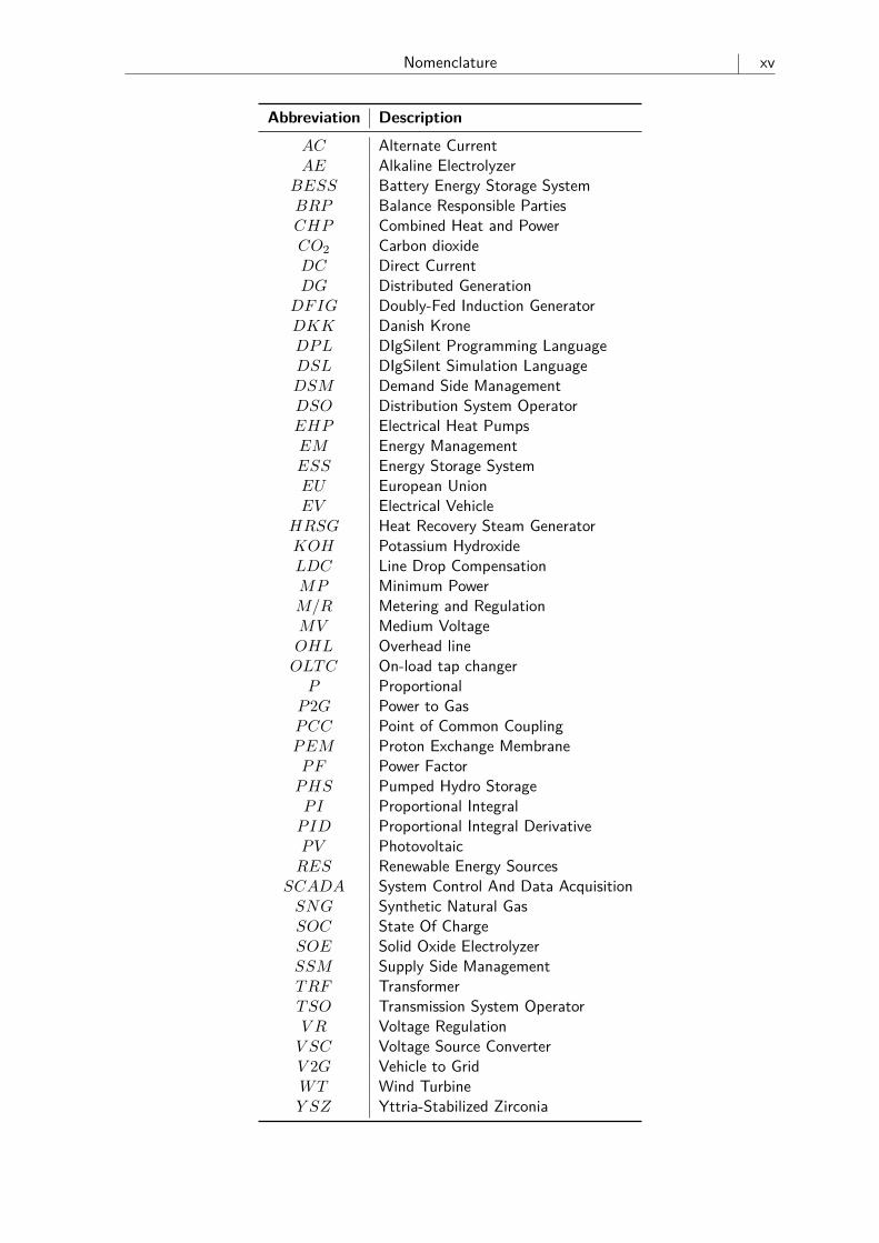
Abbreviation DescriptionAC Alternate CurrentAE Alkaline Electrolyzer
BESS Battery Energy Storage SystemBRP Balance Responsible PartiesCHP Combined Heat and PowerCO2 Carbon dioxideDC Direct CurrentDG Distributed GenerationDFIG Doubly-Fed Induction GeneratorDKK Danish KroneDPL DIgSilent Programming LanguageDSL DIgSilent Simulation LanguageDSM Demand Side ManagementDSO Distribution System OperatorEHP Electrical Heat PumpsEM Energy ManagementESS Energy Storage SystemEU European UnionEV Electrical Vehicle
HRSG Heat Recovery Steam GeneratorKOH Potassium HydroxideLDC Line Drop CompensationMP Minimum PowerM/R Metering and RegulationMV Medium VoltageOHL Overhead lineOLTC On-load tap changerP ProportionalP2G Power to GasPCC Point of Common CouplingPEM Proton Exchange MembranePF Power FactorPHS Pumped Hydro StoragePI Proportional IntegralPID Proportional Integral DerivativePV PhotovoltaicRES Renewable Energy Sources
SCADA System Control And Data AcquisitionSNG Synthetic Natural GasSOC State Of ChargeSOE Solid Oxide ElectrolyzerSSM Supply Side ManagementTRF TransformerTSO Transmission System OperatorV R Voltage RegulationV SC Voltage Source ConverterV 2G Vehicle to GridWT Wind TurbineY SZ Yttria-Stabilized Zirconia

Contents xvii
ContentsPreface iii
Abstract v
vii
xi
Nomenclature xiii
Contents xvii
1 Introduction 11.1 Background . . . . . . . . . . . . . . . . . . . . . . . . . . . . . . . . . . . . . 11.2 Problem Formulation . . . . . . . . . . . . . . . . . . . . . . . . . . . . . . . . 41.3 Objectives . . . . . . . . . . . . . . . . . . . . . . . . . . . . . . . . . . . . . . 51.4 Methodology . . . . . . . . . . . . . . . . . . . . . . . . . . . . . . . . . . . . . 51.5 Limitations . . . . . . . . . . . . . . . . . . . . . . . . . . . . . . . . . . . . . . 61.6 Outline of the Thesis . . . . . . . . . . . . . . . . . . . . . . . . . . . . . . . . 6
2 State of Art 92.1 Danish Power System . . . . . . . . . . . . . . . . . . . . . . . . . . . . . . . . 92.2 Danish Electricity Market . . . . . . . . . . . . . . . . . . . . . . . . . . . . . . 112.3 Smart Energy System . . . . . . . . . . . . . . . . . . . . . . . . . . . . . . . . 122.4 District Heating in Denmark . . . . . . . . . . . . . . . . . . . . . . . . . . . . 132.5 Danish Gas Network . . . . . . . . . . . . . . . . . . . . . . . . . . . . . . . . . 152.6 Power to Gas Technology . . . . . . . . . . . . . . . . . . . . . . . . . . . . . . 16
3 Integration of P2G in a Distribution Grid - Steady State Analysis 193.1 Grid Architecture . . . . . . . . . . . . . . . . . . . . . . . . . . . . . . . . . . 193.2 Steady State Analysis . . . . . . . . . . . . . . . . . . . . . . . . . . . . . . . . 233.3 Conclusions . . . . . . . . . . . . . . . . . . . . . . . . . . . . . . . . . . . . . 37
4 Dynamic Model Implementation in DIgSILENT PowerFactory 414.1 Modeling of the Loads . . . . . . . . . . . . . . . . . . . . . . . . . . . . . . . . 414.2 Modeling of the Wind Turbines . . . . . . . . . . . . . . . . . . . . . . . . . . . 424.3 Modeling of the CHP Plant . . . . . . . . . . . . . . . . . . . . . . . . . . . . . 454.4 Modeling of the Line Drop Compensation and Tap Changer Controller . . . . . . 514.5 Modeling of the Alkaline Electrolyzer . . . . . . . . . . . . . . . . . . . . . . . . 534.6 Modeling of the Hydrogen Storage . . . . . . . . . . . . . . . . . . . . . . . . . 594.7 Conclusions . . . . . . . . . . . . . . . . . . . . . . . . . . . . . . . . . . . . . 60
5 Voltage Support from P2G Systems - Dynamic Analysis 615.1 Base Case . . . . . . . . . . . . . . . . . . . . . . . . . . . . . . . . . . . . . . 615.2 Voltage Support from OLTC . . . . . . . . . . . . . . . . . . . . . . . . . . . . 645.3 Voltage Support from Reactive Power Dispatch . . . . . . . . . . . . . . . . . . 685.4 Voltage Support from Alkaline Electrolyzers . . . . . . . . . . . . . . . . . . . . 72
List of Figures
List of Tables
xviii Application of Power to Gas (P2G) Systems in Danish Electric Distribution Networks
5.5 Conclusions . . . . . . . . . . . . . . . . . . . . . . . . . . . . . . . . . . . . . 80
6 Energy Management from P2G Systems - Market and Dynamic Analysis 836.1 Market Strategy - Steady State Analysis . . . . . . . . . . . . . . . . . . . . . . 836.2 Dynamic Analysis . . . . . . . . . . . . . . . . . . . . . . . . . . . . . . . . . . 996.3 Conclusions . . . . . . . . . . . . . . . . . . . . . . . . . . . . . . . . . . . . . 104
7 Conclusions and Future Work 1077.1 Conclusion . . . . . . . . . . . . . . . . . . . . . . . . . . . . . . . . . . . . . . 1077.2 Future Work . . . . . . . . . . . . . . . . . . . . . . . . . . . . . . . . . . . . . 109
Appendices 111
A Electricity and Gas Market 113A.1 Electricity Market . . . . . . . . . . . . . . . . . . . . . . . . . . . . . . . . . . 113A.2 Gas Market . . . . . . . . . . . . . . . . . . . . . . . . . . . . . . . . . . . . . 116
B Data of the Elements of the Grid 117B.1 Network Elements Data . . . . . . . . . . . . . . . . . . . . . . . . . . . . . . . 117B.2 Wind Turbine Data and Modeling . . . . . . . . . . . . . . . . . . . . . . . . . 119B.3 CHP Models and Data . . . . . . . . . . . . . . . . . . . . . . . . . . . . . . . 120B.4 Alkaline Electrolyzer Model . . . . . . . . . . . . . . . . . . . . . . . . . . . . . 122
C Additional Simulations 123
D Fuzzy Logic Controller 125
Bibliography 127
Chapter 1 - Introduction 1
1 IntroductionIn this chapter the investigation done is contextualized, and the most relevant topics are presented.A short review introduces the current situation of renewable energy and discusses the possiblesolutions for their extensive implementation. The scope is further focused on the Power-to-Gastechnology, as a promising storage in the Danish energy system. Besides, a literature reviewconcerning the technical applications of this technology is presented. Subsequently, the scopeand objectives of the project are stated, followed by the used methodology to solve the presentedissues and finally the outline of the thesis.
1.1 BackgroundDuring the 20th century, energy demand has been covered by the relatively cheap and availablefossil fuels. Nevertheless, the growing energy demand together with the increasing fuel pricesare expected to bring along price uncertainty and dependence in countries without fuel resources.In this context, the Danish government has developed an energy strategy with the main targetto become fossil fuel free by 2050, which also responds according to the growing internationalconcern about CO2 emissions and climate change [1].
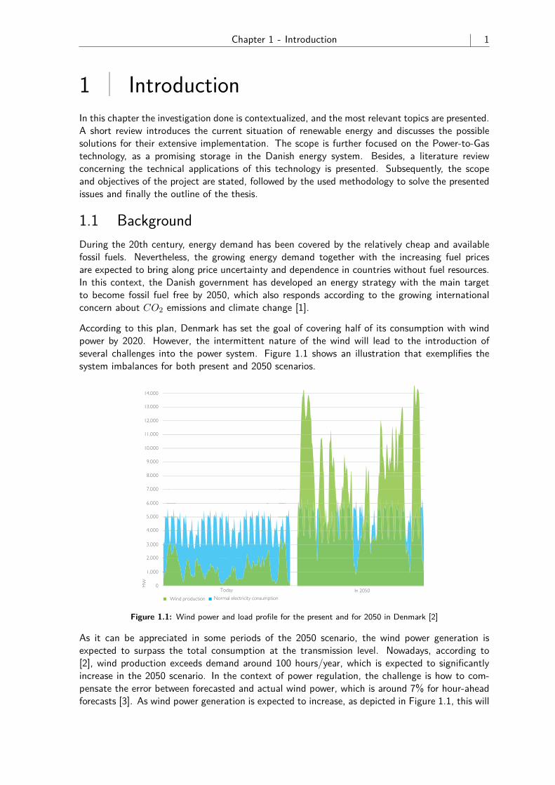
According to this plan, Denmark has set the goal of covering half of its consumption with windpower by 2020. However, the intermittent nature of the wind will lead to the introduction ofseveral challenges into the power system. Figure 1.1 shows an illustration that exemplifies thesystem imbalances for both present and 2050 scenarios.
2. Energy markets must be prepared for smart grid solutionsSmart Grid Strategy 15
0
1.000
2.000
3.000
4.000
5.000
6.000
MW
0
1.000
2.000
3.000
4.000
5.000
6.000
7.000
MW
8.000
9.000
10.000
11.000
12.000
13.000
14.000
Today In 2020 In 2050
Wind production Normal electricity consumption Wind production
2.
Energy markets must be prepared for smart grid solutions
2.1 The transmission system – balancing wind power production and electricity consumption
The primary challenge of the transmission system is that wind energy will meet 50% of traditional annual electricity consumption in 2020. Figure 4 shows fluctuations in tradi-tional electricity consumption and wind power production today and in the future. As is evident from the figure, there are no major changes in traditional electricity consumption
Flexible consumption can help resolve future challenges in the electricity grid. Here it is important to distin-guish between challenges in the transmission system and challenges in the distribution systems. The system operator responsible for the transmission system must balance an electricity system with considerably grea-ter amounts of wind power, while the grid companies responsible for distribution will have increasing pro-blems with congestion in local grids, and they will have to incorporate local electricity production from e.g. photovoltaic solar modules. If flexible consumption is to become a reality and help meet these challenges, the electricity market must be able to manage the new flexibility services as alternatives to e.g. regulating power in connection with thermal power plants in the transmission system and grid reinforcement in the distribution system.
up to 2050, because the increased electricity consumption following from a greater number of household appliances is balanced out by these appliances being more energy effi-cient. The new electricity consumption from heat pumps and electric cars, in particular, has not been included in the figure, because the consumption pattern of these techno-logies depends on whether the potential for flexible con-sumption is utilised.
On the other hand, wind power production increases considerably in 2020 and beyond. It will exceed traditional electricity consumption to a far higher extent than today. However, there will remain periods when wind power cannot meet the full demand. Energinet.dk is responsible for maintaining a balance between supply and demand in the transmission system. Large-scale and small-scale CHP plants and international connections help ensure this.
In future, flexible electricity consumption can help spur the development of new, cheap services for balancing the elec-tricity system, including regulating power. Today, regulating power is primarily delivered via international connections. Adjusting electricity consumption relative to wind power production can also enhance the market value of wind power at times when demand would otherwise be low.
Figure 4
Today
Normal electricity consumption
Figure 1.1: Wind power and load profile for the present and for 2050 in Denmark [2]
As it can be appreciated in some periods of the 2050 scenario, the wind power generation isexpected to surpass the total consumption at the transmission level. Nowadays, according to[2], wind production exceeds demand around 100 hours/year, which is expected to significantlyincrease in the 2050 scenario. In the context of power regulation, the challenge is how to com-pensate the error between forecasted and actual wind power, which is around 7% for hour-aheadforecasts [3]. As wind power generation is expected to increase, as depicted in Figure 1.1, this will
2 Application of Power to Gas (P2G) Systems in Danish Electric Distribution Networks
lead to a bigger requirement of regulation power and reserve capacity by the Danish Transmis-sion System Operator (TSO), Energinet.dk. Traditionally, in Denmark, regulation power has beensupplied by dispatchable large-scale and small-scale Combined Heat and Power (CHP) plants and,mainly, international connections [2]. However, the decommissioning of the large-scale units willlead to a further decrease in the capacity of the reserves.
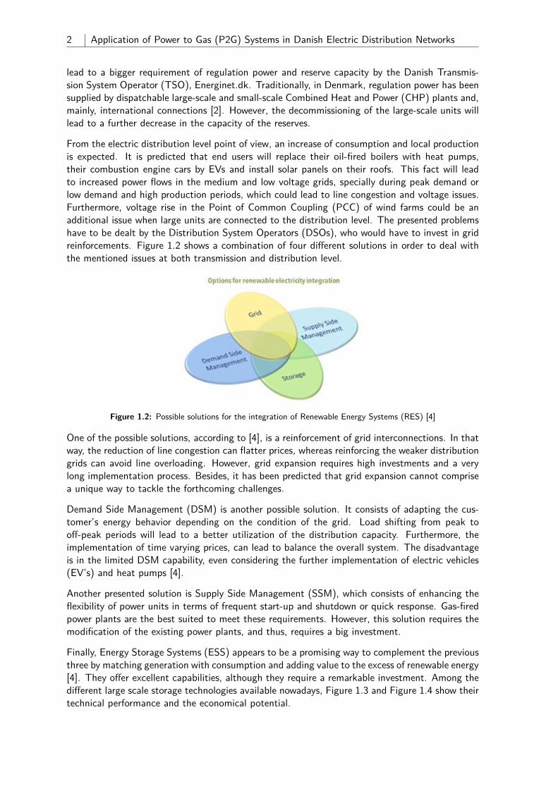
From the electric distribution level point of view, an increase of consumption and local productionis expected. It is predicted that end users will replace their oil-fired boilers with heat pumps,their combustion engine cars by EVs and install solar panels on their roofs. This fact will leadto increased power flows in the medium and low voltage grids, specially during peak demand orlow demand and high production periods, which could lead to line congestion and voltage issues.Furthermore, voltage rise in the Point of Common Coupling (PCC) of wind farms could be anadditional issue when large units are connected to the distribution level. The presented problemshave to be dealt by the Distribution System Operators (DSOs), who would have to invest in gridreinforcements. Figure 1.2 shows a combination of four different solutions in order to deal withthe mentioned issues at both transmission and distribution level.
Figure 1.2: Possible solutions for the integration of Renewable Energy Systems (RES) [4]
One of the possible solutions, according to [4], is a reinforcement of grid interconnections. In thatway, the reduction of line congestion can flatter prices, whereas reinforcing the weaker distributiongrids can avoid line overloading. However, grid expansion requires high investments and a verylong implementation process. Besides, it has been predicted that grid expansion cannot comprisea unique way to tackle the forthcoming challenges.
Demand Side Management (DSM) is another possible solution. It consists of adapting the cus-tomer’s energy behavior depending on the condition of the grid. Load shifting from peak tooff-peak periods will lead to a better utilization of the distribution capacity. Furthermore, theimplementation of time varying prices, can lead to balance the overall system. The disadvantageis in the limited DSM capability, even considering the further implementation of electric vehicles(EV’s) and heat pumps [4].
Another presented solution is Supply Side Management (SSM), which consists of enhancing theflexibility of power units in terms of frequent start-up and shutdown or quick response. Gas-firedpower plants are the best suited to meet these requirements. However, this solution requires themodification of the existing power plants, and thus, requires a big investment.
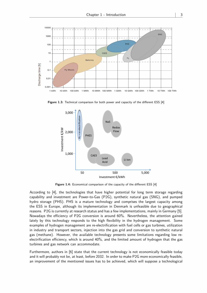
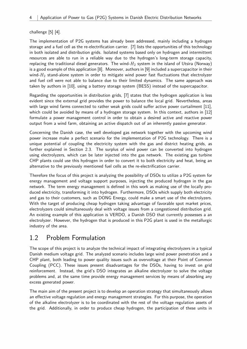
Finally, Energy Storage Systems (ESS) appears to be a promising way to complement the previousthree by matching generation with consumption and adding value to the excess of renewable energy[4]. They offer excellent capabilities, although they require a remarkable investment. Among thedifferent large scale storage technologies available nowadays, Figure 1.3 and Figure 1.4 show theirtechnical performance and the economical potential.
Chapter 1 - Introduction 3
Figure 1.3: Technical comparison for both power and capacity of the different ESS [4]
D 2.1 / Final / PU – Public
Grant agreement no. 41/65 8 AUGUST 2013
303417
Figure 13: Relative investment for various electricity storage systems (based on [Hotellier 2012])
The broad range of potential usages of hydrogen does not only mean that hydrogen
can serve several markets in parallel enabling the exploitation of synergy effects, but
also that a diversification of intrinsic business models in line with the reduction of
existing market risks can be achieved.
Figure 14 summarizes the achievable prices for hydrogen in different applications.
Based on the assumption that hydrogen in the transport sector can be sold in a
bandwidth between 6 €/kgH2 (hydrogen delivered to refuelling station) and 8 €/ kgH2
(accepted hydrogen sales price at the refuelling station for end users), it is revealed
that hydrogen as a fuel provides the most valuable sales pathway. The other
utilisation pathways may, in fact, offer a larger potential in light of volume, but their
potential with regard to economic opportunities is clearly below that of the
transportation sector.
PHES
NaS
RedoxFlow
CAESLeadAcid
Li Ion
3,000
2,000
1,000
Inve
stm
ent
€/k
W
Investment €/kWh
50 500 5,000
H2
+ re
-ele
ctri
fica
tio
n
Figure 1.4: Economical comparison of the capacity of the different ESS [4]
According to [4], the technologies that have higher potential for long term storage regardingcapability and investment are Power-to-Gas (P2G), synthetic natural gas (SNG), and pumpedhydro storage (PHS). PHS is a mature technology and comprises the largest capacity amongthe ESS in Europe, although its implementation in Denmark is unfeasible due to geographicalreasons. P2G is currently at research status and has a few implementations, mainly in Germany [5].Nowadays the efficiency of P2G conversion is around 60%. Nevertheless, the attention gainedlately by this technology responds to the high flexibility in the hydrogen management. Someexamples of hydrogen management are re-electrification with fuel cells or gas turbines, utilizationin industry and transport sectors, injection into the gas grid and conversion to synthetic naturalgas (methane). However, the available technology presents some limitations regarding low re-electrification efficiency, which is around 40%, and the limited amount of hydrogen that the gasturbines and gas network can accommodate.
Furthermore, authors in [6] state that the current technology is not economically feasible todayand it will probably not be, at least, before 2032. In order to make P2G more economically feasible,an improvement of the mentioned issues has to be achieved, which will suppose a technological
4 Application of Power to Gas (P2G) Systems in Danish Electric Distribution Networks
challenge [5] [4].
The implementation of P2G systems has already been addressed, mainly including a hydrogenstorage and a fuel cell as the re-electrification carrier. [7] lists the opportunities of this technologyin both isolated and distribution grids. Isolated systems based only on hydrogen and intermittentresources are able to run in a reliable way due to the hydrogen’s long-term storage capacity,replacing the traditional diesel generators. The wind-H2 system in the island of Utsira (Norway)is a good example of this application [8]. Moreover, authors in [9] included a supercapacitor in theirwind-H2 stand-alone system in order to mitigate wind power fast fluctuations that electrolyzerand fuel cell were not able to balance due to their limited dynamics. The same approach wastaken by authors in [10], using a battery storage system (BESS) instead of the supercapacitor.
Regarding the opportunities in distribution grids, [7] states that the hydrogen application is lessevident since the external grid provides the power to balance the local grid. Nevertheless, areaswith large wind farms connected to rather weak grids could suffer active power curtailment [11],which could be avoided by means of a hydrogen storage system. In this context, authors in [12]formulate a power management control in order to obtain a desired active and reactive poweroutput from a wind farm, obtaining an active dispatch out of an inherently passive generator.
Concerning the Danish case, the well developed gas network together with the upcoming windpower increase make a perfect scenario for the implementation of P2G technology. There is aunique potential of coupling the electricity system with the gas and district heating grids, asfurther explained in Section 2.3. The surplus of wind power can be converted into hydrogenusing electrolyzers, which can be later injected into the gas network. The existing gas turbineCHP plants could use this hydrogen in order to convert it to both electricity and heat, being analternative to the previously mentioned fuel cells as the re-electrification carrier.
Therefore the focus of this project is analyzing the possibility of DSOs to utilize a P2G system forenergy management and voltage support purposes, injecting the produced hydrogen in the gasnetwork. The term energy management is defined in this work as making use of the locally pro-duced electricity, transforming it into hydrogen. Furthermore, DSOs which supply both electricityand gas to their customers, such as DONG Energy, could make a smart use of the electrolyzers.With the target of producing cheap hydrogen taking advantage of favorable spot market prices,electrolyzers could simultaneously deal with voltage issues from a congestioned distribution grid.An existing example of this application is VERDO, a Danish DSO that currently possesses a anelectrolyzer. However, the hydrogen that is produced in this P2G plant is used in the metallurgicindustry of the area.
1.2 Problem FormulationThe scope of this project is to analyze the technical impact of integrating electrolyzers in a typicalDanish medium voltage grid. The analyzed scenario includes large wind power penetration and aCHP plant, both leading to power quality issues such as overvoltage at their Point of CommonCoupling (PCC). These issues present disadvantages for the DSOs, having to invest on gridreinforcement. Instead, the grid’s DSO integrates an alkaline electrolyzer to solve the voltageproblems and, at the same time provide energy management services by means of absorbing anyexcess generated power.
The main aim of the present project is to develop an operation strategy that simultaneously allowsan effective voltage regulation and energy management strategies. For this purpose, the operationof the alkaline electrolyzer is to be coordinated with the rest of the voltage regulation assets ofthe grid. Additionally, in order to produce cheap hydrogen, the participation of these units in
Chapter 1 - Introduction 5
the electricity wholesale markets is analyzed as part of the energy management strategy. Theproduced hydrogen is assumed to be injected into the natural gas network of the DSO company,limited by the volume percentage restriction in the Danish gas network. Further re-electrificationor heat generation from the produced hydrogen is not in the scope of this project.
1.3 ObjectivesThe main aim of the project is to analyze the feasibility of implementing P2G in a distributiongrid and developing a market strategy that provides both voltage regulation and energy manage-ment services. This strategy intends to use the electrolyzers in combination with typical voltageregulation assets in order to support a high penetration of wind power from a Danish wind farm.The realization of this involves the following:
• Steady state analysis of the impact of integrating one or more electrolyzers in a typicalDanish medium voltage grid as a mean of energy storage.
• Development of a dynamic model of the electrolyzer to provide voltage regulation, includingits operational constraints and reactive power control.
• Development of simplifications of the district heating and gas networks, in order to assesstheir impact in the electrical distribution grid and the feasibility of the hydrogen bleedingstrategy.
• Assess the capabilities and weaknesses of the electrolyzer in providing voltage regulation.
• Integrate the alkaline electrolyzer together with the typical voltage regulation assests of adistribution grid
• Technical analysis of the electrolyzer’s participation in the Elspot, Elbas and regulationmarkets in order to develop a sub-optimal market strategy for the electrolyzer.
• Development of an operation strategy of the P2G system that integrates the market strategytogether with an effective voltage regulation and energy management.
1.4 MethodologyThe main tool for the development of this project has been DIgSILENT PowerFactory. Firstly,the steady state analysis of the case study grid has been realized in this program, performing loadflow simulations which use Newton Raphson as a calculation method. The development of thedynamic models of several grid elements has also been implemented using this tool, employingDSL modules. Finally, RMS simulations have been utilized to assess their time-varying behavior.On the other hand, Matlab/Simulink has been used to analyze and create input data for theimplemented grid in PowerFactory.
Regarding the applied methodology, it is summarized as following:
• A load flow analysis is performed in the case study grid to assess the capability of theimplemented systems to provide voltage regulation under different situations. In this way abetter understanding of the regulation capacity of this units is gained, as well as the gridbehavior. Additionally, this analysis is utilized to determine the dimension and location ofthe implemented P2G system.
6 Application of Power to Gas (P2G) Systems in Danish Electric Distribution Networks
• The dynamic models of the elements of the case study grid are developed or enhanced. Theregulating control of the units has been implemented by following voltage - power factordroops. Additionally, their coordination is set depending on voltage regulation priorities.
• Time-varying simulations have been used to represent the dynamic behavior of the system,comparing the different voltage regulating elements.
• An energy management strategy is developed, determining the operation of the P2G systemdepending on the grid situation and the market’s price. This strategy is implemented usinga fuzzy logic controller.
1.5 LimitationsThe considered limitations of this project are the following:
• The operation of the switches of the case study grid is disregarded; thus, the analysis iscarried out considering the topology of the grid to be radial.
• The model of the wind turbines is simplified to a passive generator, not taking into consid-eration the dynamics of the wind power curve, shaft and blade angle control.
• The model of the line drop compensation assumes as known both the loads and the CHPplant behavior.
• The modeling of district heating, gas network and hydrogen storage are very simplified. Theassociated delays related to their dynamics are not taken into account.
• It is assumed that the alkaline electrolyzer plant is situated in a remote place and thus, notable to be connected to the transmission gas network.
• The DSO is assumed to possess the necessary forecasting and decision making tools in orderto implement the proposed market strategy.
• Load flow estimations are used in order to represent the error of real forecasts. They onlyinclude the wind power error.
• A complete cost/benefit analysis of the market strategy is not carried out.
1.6 Outline of the ThesisThe structure of the project consists of several chapters, they are summarized as it follows:
Chapter 1 - Introduction: In this chapter the background information of the chosen topic isintroduced and contextualized according to the Danish case. The scope of the project and theconsidered limitations are presented. Moreover, the methodology used is explained.
Chapter 2 - State of Art: This consists of a literature review to investigate the most relevanttopics for the project. These are presented in the form of a state of the art analysis. Being themain focus of the project, the electrolyzers as well as the Power to Gas (P2G) technology arepresented. Additionally, the Danish electricity market is investigated. Finally, the characteristicsof both the electrical distribution grid and gas network in Denmark are presented.
Chapter 1 - Introduction 7
Chapter 3 - Integration of P2G in a Distribution Grid - Steady State Analysis: In thischapter the chosen distribution grid is modeled and analyzed in the software PowerFactory, per-forming load flow simulations. The integration of the new elements of the grid such as the OLTC,reactive power control of DGs and electrolyzers is presented in this chapter.
Chapter 4 - Dynamic Model Implementation in DIgSILENT PowerFactory: In this chapterthe dynamic behavior of the wind turbines, CHP plant, OLTC and alkaline electrolyzer is modeled.The operation of each model is explained and verified.
Chapter 5 - Voltage Support from P2G Systems - Dynamic Analysis: The grid operation isanalyzed with the implementation of the dynamic models presented in Chapter 4. The contributionof the several elements to provide voltage regulation is assessed and compared.
Chapter 6 - Energy Management from P2G - Dynamic Analysis: The market strategyfor the energy management of the alkaline electrolyzers is presented in this chapter. Severalsimulations are included to show the new behavior of the system, comparing the results with theones obtained in Chapter 5.
Chapter 7 - Conclusions and Future Work: The summary and conclusions of the project arepresented in this chapter. Additionally, the possible future work based on this project is discussed.

Chapter 2 - State of Art 9
2 State of ArtIn this chapter a literature review of the most relevant topics of the project is presented. TheDanish electricity grid and its market are analyzed; the smart energy system is introduced, fol-lowed by the district heating network and the structure of the gas network; and finally, the P2Gtechnology is explained.
2.1 Danish Power SystemThe Danish power grid is divided in two areas: West Denmark and East Denmark. The firstcomprises the peninsula of Jutland and the island of Funen and is connected to Germany throughan AC overhead line (OHL) and to Norway through several DC cables. The East Denmark regionis connected to West Denmark and Germany through a DC cable and to Sweden through an ACcable. Consequently, West Denmark is part of the European grid and East Denmark is part ofthe Nordic grid. These two Danish systems are inter-connected through a DC cable since 2010,meaning they are asynchronous.
Furthermore, the Danish electricity grid is divided in two levels according to the voltage. Theseare Transmission, consisting of the networks from 400 kV to 60 kV, and Distribution, includingnetworks from 60 kV to 0.4 kV [13].
2.1.1 Transmission GridThe Danish transmission grid is owned and operated by Energinet.dk, a governmental companythat has the role of Danish Transmission System Operator (TSO). Its main responsibilities aremaintaining security of supply, planning and developing the transmission grid according to futurescenarios, supporting green energy production technologies and balancing the production andconsumption. Additionally, Energinet.dk is co-owner of the interconnections with Sweden, Norwayand Germany.
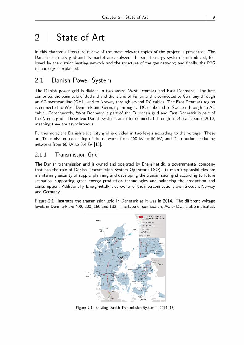
Figure 2.1 illustrates the transmission grid in Denmark as it was in 2014. The different voltagelevels in Denmark are 400, 220, 150 and 132. The type of connection, AC or DC, is also indicated.
Figure 2.1: Existing Danish Transmission System in 2014 [13]
10 Application of Power to Gas (P2G) Systems in Danish Electric Distribution Networks
2.1.2 Distribution GridThe distribution grid is the responsible to supply electricity to the end user, being their principalaim to provide reliable quality of supply to the customers. Its voltage levels range from 60 kVto 400 V. The different distribution systems in Denmark are operated by Distribution SystemOperators (DSO). Denmark has 92 different DSO, where the largest is DONG Energy, with morethan 1.000.000 customers [14].
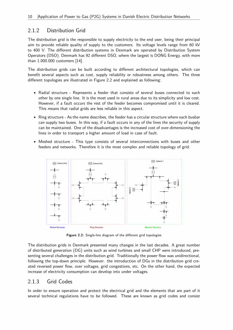
The distribution grids can be built according to different architectural topologies, which canbenefit several aspects such as cost, supply reliability or robustness among others. The threedifferent topologies are illustrated in Figure 2.2 and explained as following:
• Radial structure - Represents a feeder that consists of several buses connected to eachother by one single line. It is the most used in rural areas due to its simplicity and low cost.However, if a fault occurs the rest of the feeder becomes compromised until it is cleared.This means that radial grids are less reliable in this aspect.
• Ring structure - As the name describes, the feeder has a circular structure where each busbarcan supply two buses. In this way, if a fault occurs in any of the lines the security of supplycan be maintained. One of the disadvantages is the increased cost of over-dimensioning thelines in order to transport a higher amount of load in case of fault.
• Meshed structure - This type consists of several interconnections with buses and otherfeeders and networks. Therefore it is the most complex and reliable topology of grid.
Radial Structure Ring Structure Meshed Structure
Term inal(23)
Ter
min
al(2
2)
Term inal(19)
Term inal(18)
Term inal(17)
Ter
min
al(1
6)
Term inal(21)
Term inal(15)
Term inal(14)
Term inal(13)
Ter
min
al(1
2)T
erm
inal
(11)
Term inal(10) T erm ina l(9)
Ter
min
al(8
)
Ter
min
al(7
)
T erm ina l(6)T erm inal(5)
Term inal(4)
Term inal(3)
Term inal(2)
Term inal(1)
Term inal
General L..
Lin
e(1
8)
Netw
ork
3
Lin
e(1
7)
Ge
ne
ral
L..
Lin
e(1
6)
Lin
e(1
2)
General L..
Lin
e_
a
Line(15)
General L..
General L..
Lin
e(1
4)
Line(13)
Netw
ork
2
Ge
ne
ral
L..
Network 1
2-W
ind
ing
..
Line(11)
External Grid
Ge
ne
ralL
..
2-W
ind
ing
..
Ge
ne
ralL
..
Line(10)
Lin
e(9
)
Line(8)
Line(7)
Line(6)
General L.. General L..
Ge
ne
ralL
..G
en
era
lL..General L..
Lin
e(5
)
Line(4)
LineGeneral L..
General L..
General L..
General Load
Lin
e(3
)L
ine
(2)
Lin
e(1
)
2-W
ind
ing
..
External Grid
DIgSILENT
Figure 2.2: Single-line diagram of the different grid topologies
The distribution grids in Denmark presented many changes in the last decades. A great numberof distributed generation (DG) units such as wind turbines and small CHP were introduced, pre-senting several challenges in the distribution grid. Traditionally the power flow was unidirectional,following the top-down principle. However. the introduction of DGs in the distribution grid cre-ated reversed power flow, over voltages, grid congestions, etc. On the other hand, the expectedincrease of electricity consumption can develop into under voltages.
2.1.3 Grid CodesIn order to ensure operation and protect the electrical grid and the elements that are part of itseveral technical regulations have to be followed. These are known as grid codes and consist
Chapter 2 - State of Art 11
of guidelines that plant owners, grid owners and grid operators have to comply. As Denmark isthe country taken into account in this project, the regulations to follow are mainly imposed byEnergitilsynet, which is the Danish Energy Regulatory Authority, and Energinet.dk, as the TSO.These grid codes follow the European Standard EN 50160 for what concerns voltage quality.
The aim of this project is to analyze the implementation of an alkaline electrolyzer to providevoltage support to a medium voltage grid. Therefore, one of the main specifications is theallowed voltage deviation. As the previous sources mention, the voltage deviation in medium andlow voltage is ±10%. However, as low voltage analysis is not considered in this study, a deviationof ±5% will be taken into account for the studied medium voltage grid. Therefore the consideredvoltage limit ranges from 0.95 p.u. to 1.05 p.u..
Additionally, the generating facilities should also follow the TSO requirements regarding gridconnection. These consist of specifications regarding the properties that the plants should havesuch as power factor variation for providing voltage regulation. The exact regulations depend onthe type of generating units of the studied grid, therefore the ones taken into account in thisproject are presented in detail in Chapter 3.
2.2 Danish Electricity MarketThe deregulation of the wholesale electricity market occurred in 1999. Since then, Danish marketplayers are free to offer and purchase electricity among them, which has led to an increased freecompetition. The agreements are mainly made via Nord Pool, the common market for the Nordiccountries and, less frequently, by bilateral trading. Regulating power is purchased by the TSOsin the Nordic Regulation Power Market. In Appendix A, the role of the different market players,the present Nord Pool markets (namely Elspot and Elbas) and the regulation and balancingpower markets are further explained. References [15] [16] [17] [18] [19] are used to support thisbackground information.
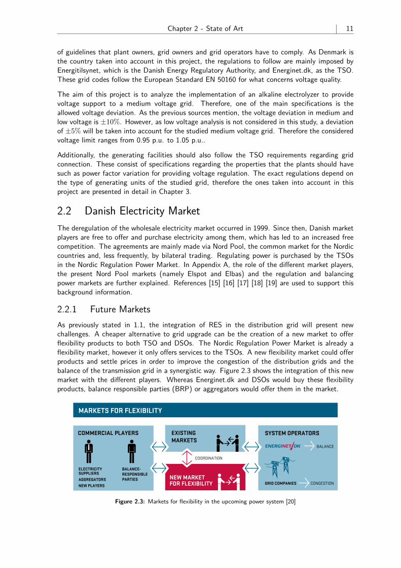
2.2.1 Future MarketsAs previously stated in 1.1, the integration of RES in the distribution grid will present newchallenges. A cheaper alternative to grid upgrade can be the creation of a new market to offerflexibility products to both TSO and DSOs. The Nordic Regulation Power Market is already aflexibility market, however it only offers services to the TSOs. A new flexibility market could offerproducts and settle prices in order to improve the congestion of the distribution grids and thebalance of the transmission grid in a synergistic way. Figure 2.3 shows the integration of this newmarket with the different players. Whereas Energinet.dk and DSOs would buy these flexibilityproducts, balance responsible parties (BRP) or aggregators would offer them in the market.
SMART GRID IN DENMARK 2.0 | 15
4 // FOCUS ON MARKET ACCESSIt is central to the concept that mobilising and activating flexibility must be market-based. This means that the private players must be free to decide to whom and to what extent they offer their flexibility, and it must be ensured that the flexibility is priced and sold transparently
The use of price signals is central to releasing the value of flexible electricity consumption and production. However, price signals are not sufficient on their own as the response to the price signals cannot be guaranteed in advance. Trading in flexibility products is the supplementary measure which ensures that specific needs for flexibility can be met at all times. The aim of the concept is therefore, in the long term, to establish an efficient market for trading in standardised flexibility products.
Today, markets have already been established where Energinet.dk procures flexibility products, for example the common Nordic regulating power market (NOIS). However, there is no similar trading platform which allows the grid companies to utilise flexibility products as an alternative to grid reinforcements.
tWo DiFFErEnt mEchanisms – PricE signaLs anD FLEXiBiLity ProDUcts
The concept basically distinguishes between two different mechanisms for activating flexibility:
¼ PRICE SIGNALS (variable grid tariffs and electricity prices), providing a general incentive for customers to shift their electricity consumption and production to times which are less inconvenient for the power system.
¼ FLEXIBILITY PRODUCTS, where a service which has been clearly agreed and defined in advance – for example reducing the load in a specified grid area – can be activated as and when needed by grid companies and/or Energinet.dk at an agreed price.
BALANCE
CONGESTIONGRID COMPANIES
SYSTEM OPERATORS
BALANCE
CONGESTIONGRID COMPANIES
SYSTEM OPERATORS
BALANCE
CONGESTIONGRID COMPANIES
SYSTEM OPERATORS
COMMERCIAL PLAYERS
ELECTRICITY SUPPLIERS
AGGREGATORS
NEW PLAYERS
BALANCE-RESPONSIBLE PARTIES
PRIVATE PLAYERS
HEAT PUMPSELECTRIC VEHICLES
CUSTOMERS
MMM
OFFER REQUESTHANDLE
COMMERCIAL PLAYERS
ELECTRICITY SUPPLIERS
AGGREGATORS
NEW PLAYERS
Fig. kap3_Roller
COMMERCIAL PLAYERS
ELECTRICITY SUPPLIERS
AGGREGATORS
NEW PLAYERS
Fig. kap5_informationsmodel
BALANCE-RESPONSIBLE PARTIES
BALANCE-RESPONSIBLE PARTIES
COORDINATION
Fig. kap3_Marked
EXISTING MARKETS
NEW MARKET FOR FLEXIBILITY
COMPONENT-ORIENTED IEC 61850 ETC. (LOGICAL NODES)
SYSTEM-ORIENTEDIEC 61970 ETC. (CIM)
PRIVATE PLAYERS
HEAT PUMPSELECTRIC VEHICLES
CUSTOMERS
MMM
markEts For FLEXiBiLity
a nEW markEt for flexibility makes it possible for the grid companies to purchase flexibility products as an alternative to grid reinforcements. The new
market will be coordinated with the existing markets for flexibility, for example the regulating power market.
Figure 2.3: Markets for flexibility in the upcoming power system [20]
12 Application of Power to Gas (P2G) Systems in Danish Electric Distribution Networks
BRPs placed in congested distribution grids could gain extra benefit by taking part in the newmarket. For instance, a producer could decrease its output for avoiding lines overloading, if themarket prices are attractive enough to change its schedule. In the context of this project, anelectrolyzer placed in a distribution grid with high wind power penetration can provide voltageregulation and help avoiding local bottlenecks. When operated by the DSO, the target would beto correct the possible voltage deviation, minimizing the impact in the schedule.
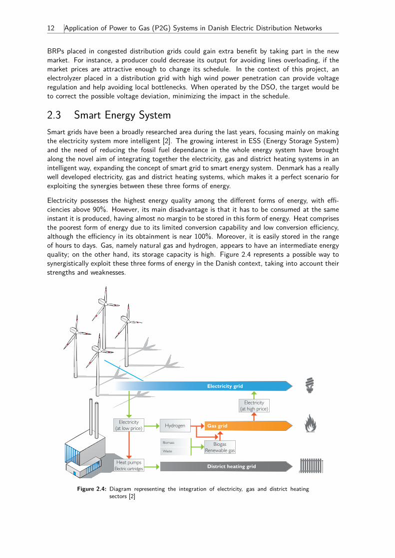
2.3 Smart Energy SystemSmart grids have been a broadly researched area during the last years, focusing mainly on makingthe electricity system more intelligent [2]. The growing interest in ESS (Energy Storage System)and the need of reducing the fossil fuel dependance in the whole energy system have broughtalong the novel aim of integrating together the electricity, gas and district heating systems in anintelligent way, expanding the concept of smart grid to smart energy system. Denmark has a reallywell developed electricity, gas and district heating systems, which makes it a perfect scenario forexploiting the synergies between these three forms of energy.
Electricity possesses the highest energy quality among the different forms of energy, with effi-ciencies above 90%. However, its main disadvantage is that it has to be consumed at the sameinstant it is produced, having almost no margin to be stored in this form of energy. Heat comprisesthe poorest form of energy due to its limited conversion capability and low conversion efficiency,although the efficiency in its obtainment is near 100%. Moreover, it is easily stored in the rangeof hours to days. Gas, namely natural gas and hydrogen, appears to have an intermediate energyquality; on the other hand, its storage capacity is high. Figure 2.4 represents a possible way tosynergistically exploit these three forms of energy in the Danish context, taking into account theirstrengths and weaknesses.
4. Smart Energy – wind power in the district heating and gas sectorsSmart Grid Strategy 27
As part of the government’s innovation strategy, in Decem-ber 2012 the Ministry of Climate, Energy and Building launched a pilot partnership on smart energy with broad involvement from the energy sector. There is already consi-derable activity within the smart grid and there is a fledgling interest from the energy sector, RDD institutes and the business community in developing towards smart energy. However, a fundamental challenge for development of smart energy is that the solutions involve many players and sectors which do not usually work closely together. The
4.
Smart Energy – wind power in the district heating and gas sectors
The smart grid agenda has so far primarily focussed on intelligent electricity systems, but in future the smart grid should also be incorporated into the gas and district heating grids as part of an integrated smart energy system. Denmark has extremely well developed district heating and gas grids and therefore there is a good basis to exploit the synergies between the different types of energy and grid. For example, the district heating and gas systems can be used to store electricity from wind power in other types of energy for later use when the price of electricity is low. The alternative to storing electricity is to export electricity abroad. However, this is not necessarily always appropriate as better integration of the electricity, heating and gas sectors can help reduce the use of fossil fuels and make up a supplement to biomass in the district heating sector.
Figure 8. When there is a lot of wind turbine electricity in the grid and the price of electricity is low, hydrogen and district heating can be produced.
BiogasRenewable gas
Electricity grid
District heating grid
Gas grid
Biomass
Waste
Electricity (at low price)
Electricity (at high price)
Heat pumpsElectric cartridges
Hydrogen
overall objective of the partnership will be to help open up narrow thinking within the electricity, heating/cooling and gas sectors. In addition the partnership is to promote and disseminate the results of demonstration activities in smart energy.
Figure 8 illustrates how the interplay between the electri-city, district heating and gas systems can be utilised becau-se of the different processes and technologies which are explained in the following section. Figure 2.4: Diagram representing the integration of electricity, gas and district heating
sectors [2]
Chapter 2 - State of Art 13
The expansion of RES involves an increase of renewable electricity production. The high vari-ability of wind or PV generation implies periods of lack or surplus of electricity. The excess ofelectricity could be transformed into hydrogen or heat, taking advantage of low spot prices. Theresponsible units for transforming electricity to heat are heat pumps and electrical cartridges,whereas electrolyzers are used to produce hydrogen. Taking into consideration the production ofhydrogen, when renewable electricity cannot cover the demand, the deficit could be supplied bythe re-electrification carriers, namely fuel cells and gas turbines.
In the context of the present work, the integration of the three energy sectors can be doneby taking into consideration the implementation of a gas turbine CHP and an electrolyzer in adistribution grid. Nevertheless, the main focus will be assessing the impact of this integrationinto the electrical system. In the following sections, both Danish district heating and gas sectorswill be further explained, as the electrical side has already been described in Section 2.1.
2.4 District Heating in DenmarkDenmark has been, for decades, the worldwide leader in district heating technologies. Heat isproduced in a centralized and local scale, being transported to the end consumers through waterpipes. Nowadays, around 63% of the Danish heat demand is supplied by its efficient district heating[21]. This heat is mostly produced in CHP plants, which consist of simultaneous production ofboth heat and electricity.
During 2012, 74.6% of the electricity production in Denmark was from CHP plants, whereas73% of the produced heat was generated together with electricity [22]. The rest of the districtheating demand was mainly produced with boilers and, in smaller amount, via electricity heatingelements, namely electrical cartridges and heat pumps. These statistics show the high levelof implementation this technology has in Denmark, both in the electricity and district heatingsystems. The scope of the present project regarding district heating will only fall within CHPplants, therefore, this will be the only technology further explained.
2.4.1 Combined Heat and Power (CHP)As mentioned previously, CHP technology consists on producing heat and electricity simultane-ously. The excess heat from conventional turbines is used in order to heat water, used in theindustry and district heating. The use of waste heat leads to achieve higher efficiency and loweremissions, compared to separate production of electricity in a conventional thermal power plantand heat in a boiler. As an example, a 5MW combined cycle CHP has an overall efficiency of75%, whereas the separate production for the same amount of heat and power has an efficiencyof only 50% [23]. As previously explained, this technology has a high degree of implementationin Denmark. Table 2.1 shows the amount of CHPs and their installed capacity in 2013, wherethe higher amount of decentralized plants can be noticed.
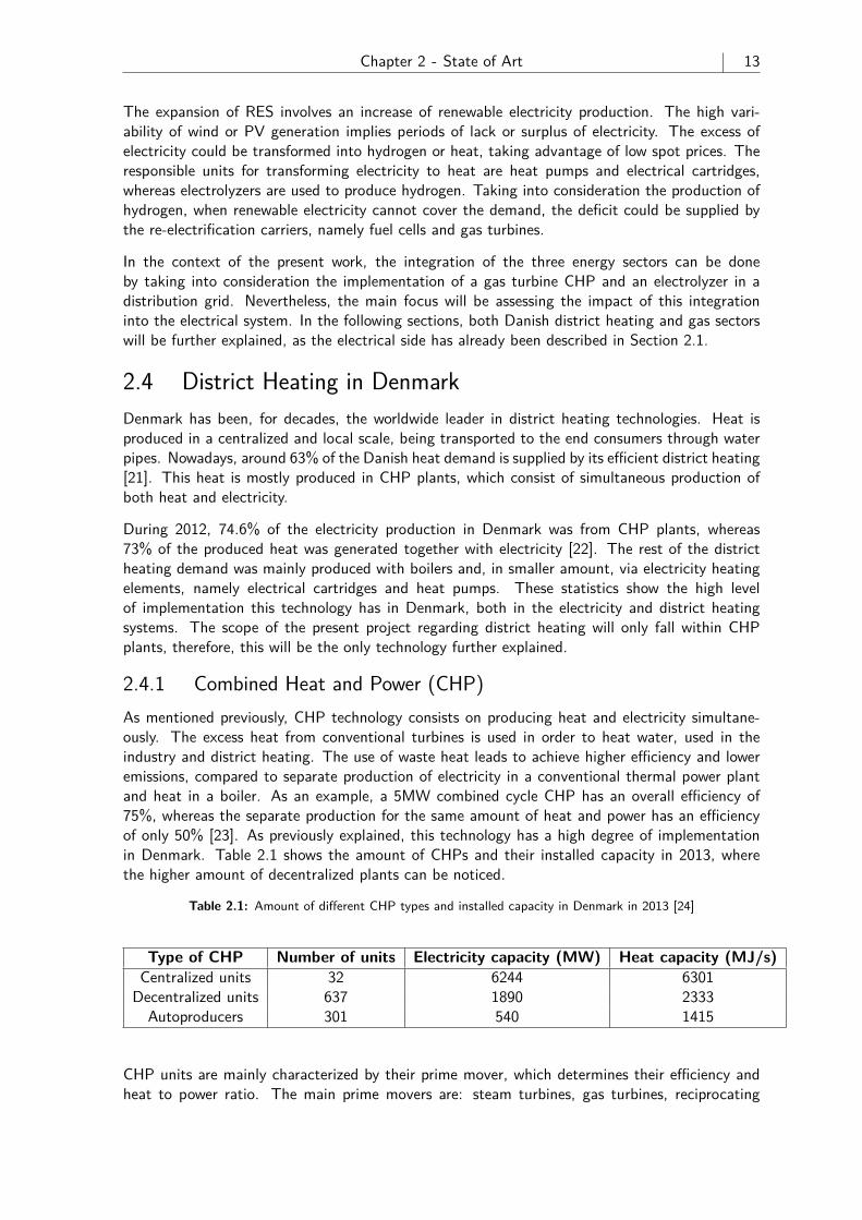
Table 2.1: Amount of different CHP types and installed capacity in Denmark in 2013 [24]
Type of CHP Number of units Electricity capacity (MW) Heat capacity (MJ/s)Centralized units 32 6244 6301Decentralized units 637 1890 2333Autoproducers 301 540 1415
CHP units are mainly characterized by their prime mover, which determines their efficiency andheat to power ratio. The main prime movers are: steam turbines, gas turbines, reciprocating
14 Application of Power to Gas (P2G) Systems in Danish Electric Distribution Networks
engines, microturbines and fuel cells [23]. However, gas turbines is the only type considered inthe present project.
In order to provide flexibility, heat and electricity are decoupled with other heating elements.These elements are heat storage and boilers (fuel-fired and electric). Excess heat is stored whenelectricity spot prices are high and operating the CHP plants is highly profitable. On the contrary,when electricity spot prices are low and producing electricity is not economically feasible, heatdemand is covered by using the boilers or heat storage, if available [25].
Gas Turbines
The main characteristics of gas turbine generators are summarized in Table 2.2, giving the valuesof efficiency, nominal power and heat to power ratio:
Table 2.2: Characteristics of gas turbine generators [23]
Typical capacity (MWe) Heat to power ratio CHP efficiency (%)0.5-300 0.6-1.1 66-71
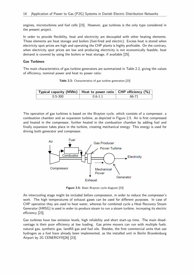
The operation of gas turbines is based on the Brayton cycle, which consists of a compressor, acombustion chamber and an expansion turbine, as depicted in Figure 2.5. Air is first compressedand heated in the compressor, further heated in the combustion chamber by adding fuel andfinally expansion takes place in the turbine, creating mechanical energy. This energy is used fordriving both generator and compressor.
Figure 2.5: Basic Brayton cycle diagram [23]
An intercooling stage might be included before compression, in order to reduce the compressor’swork. The high temperatures of exhaust gases can be used for different purposes. In case ofCHP operation they are used to heat water, whereas for combined cycle a Heat Recovery SteamGenerator (HRSG) is used in order to produce steam to run a steam turbine, increasing its electricefficiency [23].
Gas turbines have low emission levels, high reliability and short start-up time. The main disad-vantage is their poor efficiency at low loading. Gas prime movers can run with multiple fuels:natural gas, synthetic gas, landfill gas and fuel oils. Besides, the first commercial units that usehydrogen as a fuel have already been implemented, as the installed unit in Berlin BrandenburgAirport by 2G CENERGY®[26] [23].
Chapter 2 - State of Art 15
2.5 Danish Gas NetworkDenmark is one of the few countries that is not dependent on natural gas, it has its own productionof gas from the North Sea which is expected to continue until at least 2025 [27]. Furthermore,it exports gas to Sweden, Germany and The Netherlands. In 2013 the net production of naturalgas was 4 · 109Nm3, of which 47% was exported [27].
The natural gas is transported to the mainland through offshore pipelines from the productionplacements in the Danish continental shelf. Two pipelines transport the gas to Denmark andanother transports gas to The Netherlands. When the gas is onshore a treatment plant evaluatesthe quality of the gas. From there the gas is distributed to the customers, to storage facilitiesand to the neighboring countries [28].
The gas network is divided in two parts: transmission and distribution. First, the gas is transportedat more than 50bar pressure. The distribution network brings the gas to the end-user, beingtransported at lower pressures [29].
The onshore gas transmission network is owned and operated by Energinet.dk. As shown in Figure2.6, the pipelines transport the gas from north to south and west to east. Along the lines thereare meter and regulation stations (M/R) which ensure that the pressure level is the adequate.Two subterranean storage facilities are available to ensure quality of supply: Lille Torup in NorthJutland and Stenlille in Zealand, both owned by Energinet.dk [29].
Figure 2.6: The Danish transmission gas network in 2014 [30]
Gas Storage in Denmark
The limited natural gas supply coming from the North Sea results in a need of storage. In colddays the demand of natural gas can reach approximately 30−33·106Nm3/day, while the pipelinesfrom the North sea can only transport about 22− 24 · 106Nm3/day.
The storage facility of Lille Torup is placed in an underground salt dome. It consists of 7 storagecavities which range from 200-300 m high and 50-65 m wide. The total storage is 440 · 106Nm3,which corresponds to 2 months of gas consumption. Stenlille is an acquifer storage facility whichconsists of porous sandstone layers at 1500m depth. Its storage capacity is about 558 · 106Nm3.[31]
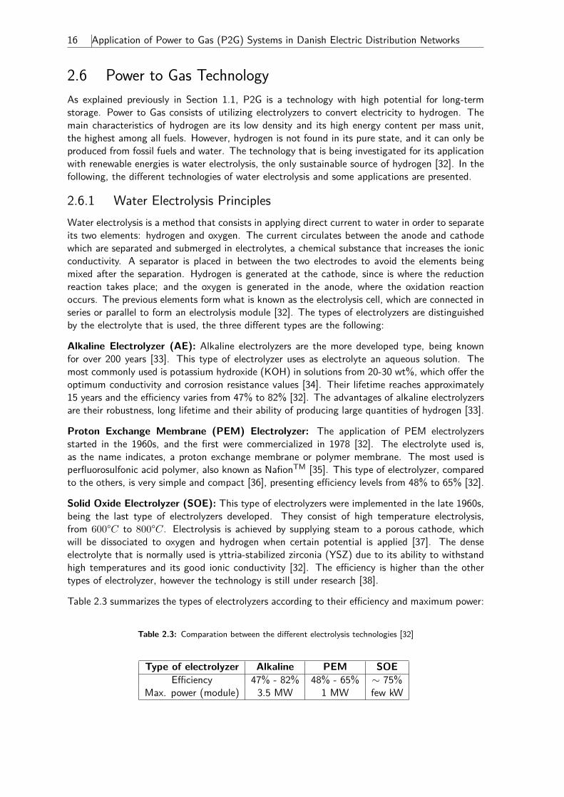
16 Application of Power to Gas (P2G) Systems in Danish Electric Distribution Networks
2.6 Power to Gas TechnologyAs explained previously in Section 1.1, P2G is a technology with high potential for long-termstorage. Power to Gas consists of utilizing electrolyzers to convert electricity to hydrogen. Themain characteristics of hydrogen are its low density and its high energy content per mass unit,the highest among all fuels. However, hydrogen is not found in its pure state, and it can only beproduced from fossil fuels and water. The technology that is being investigated for its applicationwith renewable energies is water electrolysis, the only sustainable source of hydrogen [32]. In thefollowing, the different technologies of water electrolysis and some applications are presented.
2.6.1 Water Electrolysis PrinciplesWater electrolysis is a method that consists in applying direct current to water in order to separateits two elements: hydrogen and oxygen. The current circulates between the anode and cathodewhich are separated and submerged in electrolytes, a chemical substance that increases the ionicconductivity. A separator is placed in between the two electrodes to avoid the elements beingmixed after the separation. Hydrogen is generated at the cathode, since is where the reductionreaction takes place; and the oxygen is generated in the anode, where the oxidation reactionoccurs. The previous elements form what is known as the electrolysis cell, which are connected inseries or parallel to form an electrolysis module [32]. The types of electrolyzers are distinguishedby the electrolyte that is used, the three different types are the following:
Alkaline Electrolyzer (AE): Alkaline electrolyzers are the more developed type, being knownfor over 200 years [33]. This type of electrolyzer uses as electrolyte an aqueous solution. Themost commonly used is potassium hydroxide (KOH) in solutions from 20-30 wt%, which offer theoptimum conductivity and corrosion resistance values [34]. Their lifetime reaches approximately15 years and the efficiency varies from 47% to 82% [32]. The advantages of alkaline electrolyzersare their robustness, long lifetime and their ability of producing large quantities of hydrogen [33].
Proton Exchange Membrane (PEM) Electrolyzer: The application of PEM electrolyzersstarted in the 1960s, and the first were commercialized in 1978 [32]. The electrolyte used is,as the name indicates, a proton exchange membrane or polymer membrane. The most used isperfluorosulfonic acid polymer, also known as NafionTM [35]. This type of electrolyzer, comparedto the others, is very simple and compact [36], presenting efficiency levels from 48% to 65% [32].
Solid Oxide Electrolyzer (SOE): This type of electrolyzers were implemented in the late 1960s,being the last type of electrolyzers developed. They consist of high temperature electrolysis,from 600°C to 800°C. Electrolysis is achieved by supplying steam to a porous cathode, whichwill be dissociated to oxygen and hydrogen when certain potential is applied [37]. The denseelectrolyte that is normally used is yttria-stabilized zirconia (YSZ) due to its ability to withstandhigh temperatures and its good ionic conductivity [32]. The efficiency is higher than the othertypes of electrolyzer, however the technology is still under research [38].
Table 2.3 summarizes the types of electrolyzers according to their efficiency and maximum power:
Table 2.3: Comparation between the different electrolysis technologies [32]
Type of electrolyzer Alkaline PEM SOEEfficiency 47% - 82% 48% - 65% ∼ 75%
Max. power (module) 3.5 MW 1 MW few kW
Chapter 2 - State of Art 17
2.6.2 Integration of Hydrogen in the Gas NetworkThe main issue of hydrogen production is its final use. The utilization of hydrogen for thetransportation sector implies the construction of an infrastructure to distribute it [39]. Given this,a feasible solution is injecting it to the existing gas network [40]. However, there are restrictionsregarding the materials of the pipelines and the energetic limitations of combining both gases[39]. In order to provide the same energy, the volume of hydrogen needed is three times ofthe natural gas [40], which limits the concentration of hydrogen in natural gas. However, thegreatest limitation is due to the materials of the pipelines, storage units and equipment. Theadmissible concentration of hydrogen in present natural gas systems was studied in [41]. Thisstudy concluded that most elements of the gas network admit a concentration of 10% by volumeof hydrogen. However, some elements could be deteriorated or cause adverse effects with such ahigh concentration of hydrogen. The most sensitive components are underground porous storage,steel tanks, gas engines and old gas turbines.
2.6.3 Power to Gas ApplicationsHistorically, the two largest water electrolysis plants were installed in Norway, with approximately135 MW each. The plants were supplied by hydro power, and the produced hydrogen was usedfor fertilizer production. However, these plants were closed down as hydrogen could be producedthrough other sources at a lower cost [42].
Nowadays, the focus on P2G plants is on re-utilizing the excess renewable production. Recently,these plants are being developed and installed in several countries for this purpose. Three projectsare presented in the following:
BioCat Project: A new project called P2G-BioCat is being developed in Denmark, its objectiveis to design a commercial P2G facility to provide energy storage to the Danish energy system[43]. The project is coordinated by several companies, being the most important Electrochaeaand Energinet.dk. In this case the surplus electricity from wind power is used to obtain hydrogen,which will be used to convert biogas into methane. A 1 MW water electrolysis plant, using analkaline electrolyzer from Hydrogenics, will be installed in Spildevandscenter Avedøre, one of thelargest waste-water treatment facilities. The final gas will be injected to the local distributionnetwork and the co-products, oxygen and heat, will be recycled in the waste-water plant [44].
Falkenhagen (Germany): In 2013 the energy company E-ON installed a P2G plant in Falken-hagen, Germany. It consists of a 2MW alkaline electrolyzer that converts excess electricity from awind farm to produce hydrogen. This hydrogen is injected at a rate of 360Nm3/h to the naturalgas network, at a volume rate of 2% [45].
Energie Park Mainz (Germany): A new P2G plant is planned to start operating in spring 2015in the German city of Mainz. It consists of a 6 MW PEM electrolyzer, and therefore will be thelargest plant operating on surplus electricity from wind power [46].
2.6.4 ConclusionAccording to the presented literature review, it is known that the only types of electrolyzers thatare commercialized nowadays are alkaline and PEM. However, the latter is still under development,while the alkaline electrolyzer can be considered as mature technology. As discussed in Sections2.6.3 and 2.6.1, alkaline electrolyzer plants are available up to 135 MW, offering efficiencies from47% to 82% and lifetime of 15 years. For this reason, the alkaline electrolyzer is the type that willbe taken into consideration in this project. Moreover, a PowerFactory model of alkaline electrolyzerhas been presented in [47], which can be used in this project with appropriate modifications.

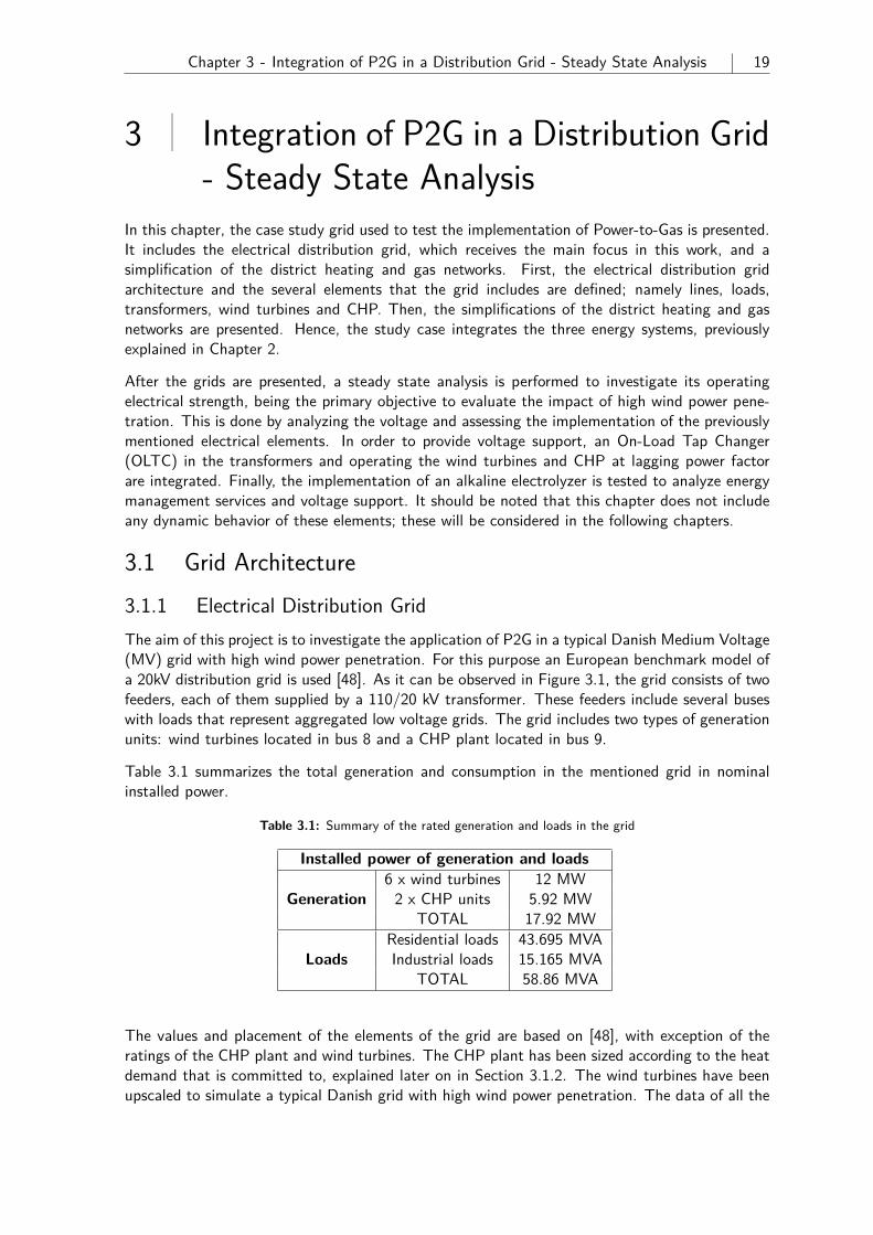
Chapter 3 - Integration of P2G in a Distribution Grid - Steady State Analysis 19
3 Integration of P2G in a Distribution Grid- Steady State Analysis
In this chapter, the case study grid used to test the implementation of Power-to-Gas is presented.It includes the electrical distribution grid, which receives the main focus in this work, and asimplification of the district heating and gas networks. First, the electrical distribution gridarchitecture and the several elements that the grid includes are defined; namely lines, loads,transformers, wind turbines and CHP. Then, the simplifications of the district heating and gasnetworks are presented. Hence, the study case integrates the three energy systems, previouslyexplained in Chapter 2.
After the grids are presented, a steady state analysis is performed to investigate its operatingelectrical strength, being the primary objective to evaluate the impact of high wind power pene-tration. This is done by analyzing the voltage and assessing the implementation of the previouslymentioned electrical elements. In order to provide voltage support, an On-Load Tap Changer(OLTC) in the transformers and operating the wind turbines and CHP at lagging power factorare integrated. Finally, the implementation of an alkaline electrolyzer is tested to analyze energymanagement services and voltage support. It should be noted that this chapter does not includeany dynamic behavior of these elements; these will be considered in the following chapters.
3.1 Grid Architecture3.1.1 Electrical Distribution GridThe aim of this project is to investigate the application of P2G in a typical Danish Medium Voltage(MV) grid with high wind power penetration. For this purpose an European benchmark model ofa 20kV distribution grid is used [48]. As it can be observed in Figure 3.1, the grid consists of twofeeders, each of them supplied by a 110/20 kV transformer. These feeders include several buseswith loads that represent aggregated low voltage grids. The grid includes two types of generationunits: wind turbines located in bus 8 and a CHP plant located in bus 9.
Table 3.1 summarizes the total generation and consumption in the mentioned grid in nominalinstalled power.
Table 3.1: Summary of the rated generation and loads in the grid
Installed power of generation and loads
Generation6 x wind turbines 12 MW2 x CHP units 5.92 MW
TOTAL 17.92 MW
LoadsResidential loads 43.695 MVAIndustrial loads 15.165 MVA
TOTAL 58.86 MVA
The values and placement of the elements of the grid are based on [48], with exception of theratings of the CHP plant and wind turbines. The CHP plant has been sized according to the heatdemand that is committed to, explained later on in Section 3.1.2. The wind turbines have beenupscaled to simulate a typical Danish grid with high wind power penetration. The data of all the
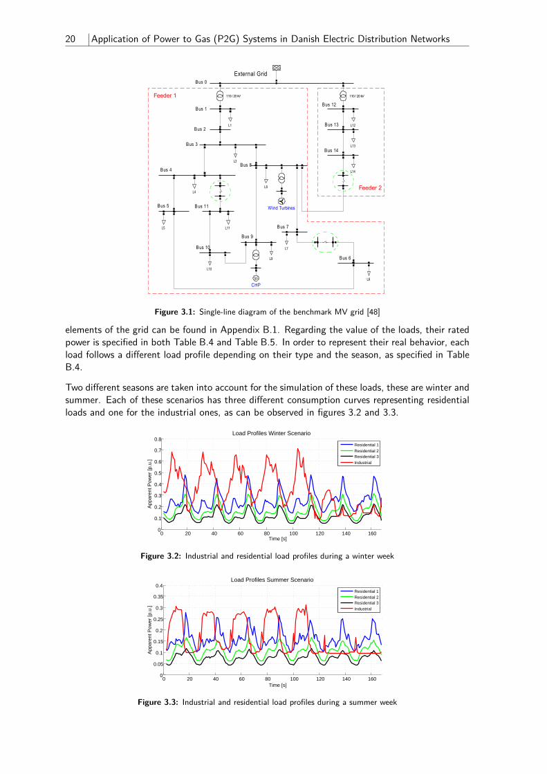
20 Application of Power to Gas (P2G) Systems in Danish Electric Distribution Networks
Feeder 1
Feeder 2
Term
inal
(8)
Terminal(7)
Terminal(6)
110 / 20 kV110 / 20 kV
Terminal(4)
Terminal(5)
Terminal(1)
Terminal
Bus 12
Bus 7
Term
inal
(3)
Bus 6
Bus 8
Bus 9
Bus 10
Bus 11
Bus 4
Bus 5
Bus 0
Bus 14
Bus 13Bus 2
Bus 3
Bus 1
Bre
ake
r/S
..
Bre
ake
r/S
..
Line(6)Line(5)
Breaker/S..
SG~
CHP
W ind Turbines
2-W
ind
ing
..
2-W
ind
ing
..
Lin
e1
4-c
OH
L
Lin
ea
-11
Ca
ble
Lin
e4
-aC
ab
le
TR
2T
RF
Line(4)
Lin
e1
3-1
4O
HL
Lin
e1
2-1
3O
HL
L12
L7
Line(3)
L6
Lin
e7
-8C
ab
le
Lin
e(2
)
L9
Line
Lin
e1
0-1
1C
ab
le
L10
L11L5
L4
Lin
e4
-5C
ab
le
Lin
e3
-4C
ab
le
External Grid
L14
L13
L8
Lin
e1
-2O
HL
Lin
e2
-3C
ab
le
Lin
e(1
)
L3
L1
TR
1T
RF
DIgSILENT
Figure 3.1: Single-line diagram of the benchmark MV grid [48]
elements of the grid can be found in Appendix B.1. Regarding the value of the loads, their ratedpower is specified in both Table B.4 and Table B.5. In order to represent their real behavior, eachload follows a different load profile depending on their type and the season, as specified in TableB.4.
Two different seasons are taken into account for the simulation of these loads, these are winter andsummer. Each of these scenarios has three different consumption curves representing residentialloads and one for the industrial ones, as can be observed in figures 3.2 and 3.3.
0 20 40 60 80 100 120 140 160
0.1
0.2
0.3
0.4
0.5
0.6
0.7
0.8Load Profiles Winter Scenario
Time [s]
App
aren
t Pow
er [p
.u.]
0
Residential 1Residential 2Residential 3Industrial
Figure 3.2: Industrial and residential load profiles during a winter week
0 20 40 60 80 100 120 140 160
0.05
0.1
0.15
0.2
0.25
0.3
0.35
0.4Load Profiles Summer Scenario
Time [s]
App
aren
t Pow
er [p
.u.]
0
Residential 1Residential 2Residential 3Industrial
Figure 3.3: Industrial and residential load profiles during a summer week
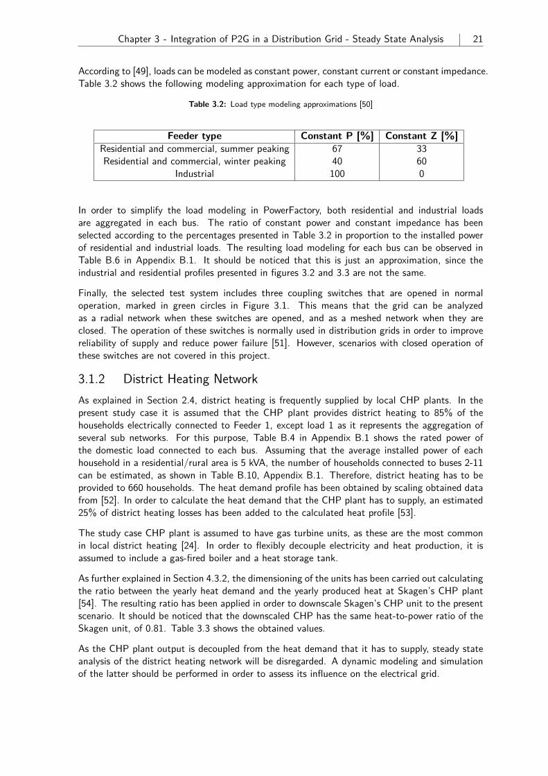
Chapter 3 - Integration of P2G in a Distribution Grid - Steady State Analysis 21
According to [49], loads can be modeled as constant power, constant current or constant impedance.Table 3.2 shows the following modeling approximation for each type of load.
Table 3.2: Load type modeling approximations [50]
Feeder type Constant P [%] Constant Z [%]Residential and commercial, summer peaking 67 33Residential and commercial, winter peaking 40 60
Industrial 100 0
In order to simplify the load modeling in PowerFactory, both residential and industrial loadsare aggregated in each bus. The ratio of constant power and constant impedance has beenselected according to the percentages presented in Table 3.2 in proportion to the installed powerof residential and industrial loads. The resulting load modeling for each bus can be observed inTable B.6 in Appendix B.1. It should be noticed that this is just an approximation, since theindustrial and residential profiles presented in figures 3.2 and 3.3 are not the same.
Finally, the selected test system includes three coupling switches that are opened in normaloperation, marked in green circles in Figure 3.1. This means that the grid can be analyzedas a radial network when these switches are opened, and as a meshed network when they areclosed. The operation of these switches is normally used in distribution grids in order to improvereliability of supply and reduce power failure [51]. However, scenarios with closed operation ofthese switches are not covered in this project.
3.1.2 District Heating NetworkAs explained in Section 2.4, district heating is frequently supplied by local CHP plants. In thepresent study case it is assumed that the CHP plant provides district heating to 85% of thehouseholds electrically connected to Feeder 1, except load 1 as it represents the aggregation ofseveral sub networks. For this purpose, Table B.4 in Appendix B.1 shows the rated power ofthe domestic load connected to each bus. Assuming that the average installed power of eachhousehold in a residential/rural area is 5 kVA, the number of households connected to buses 2-11can be estimated, as shown in Table B.10, Appendix B.1. Therefore, district heating has to beprovided to 660 households. The heat demand profile has been obtained by scaling obtained datafrom [52]. In order to calculate the heat demand that the CHP plant has to supply, an estimated25% of district heating losses has been added to the calculated heat profile [53].
The study case CHP plant is assumed to have gas turbine units, as these are the most commonin local district heating [24]. In order to flexibly decouple electricity and heat production, it isassumed to include a gas-fired boiler and a heat storage tank.
As further explained in Section 4.3.2, the dimensioning of the units has been carried out calculatingthe ratio between the yearly heat demand and the yearly produced heat at Skagen’s CHP plant[54]. The resulting ratio has been applied in order to downscale Skagen’s CHP unit to the presentscenario. It should be noticed that the downscaled CHP has the same heat-to-power ratio of theSkagen unit, of 0.81. Table 3.3 shows the obtained values.
As the CHP plant output is decoupled from the heat demand that it has to supply, steady stateanalysis of the district heating network will be disregarded. A dynamic modeling and simulationof the latter should be performed in order to assess its influence on the electrical grid.
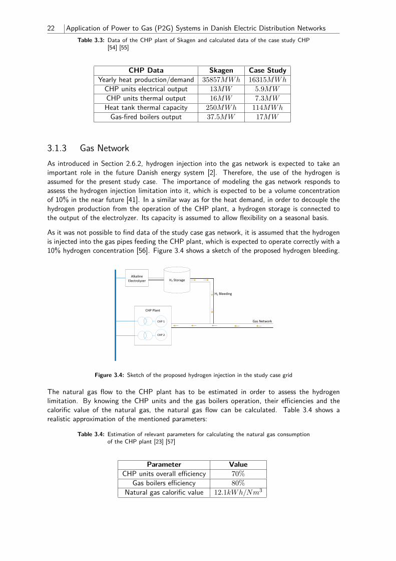
22 Application of Power to Gas (P2G) Systems in Danish Electric Distribution NetworksTable 3.3: Data of the CHP plant of Skagen and calculated data of the case study CHP
[54] [55]
CHP Data Skagen Case StudyYearly heat production/demand 35857MWh 16315MWh
CHP units electrical output 13MW 5.9MW
CHP units thermal output 16MW 7.3MW
Heat tank thermal capacity 250MWh 114MWh
Gas-fired boilers output 37.5MW 17MW
3.1.3 Gas NetworkAs introduced in Section 2.6.2, hydrogen injection into the gas network is expected to take animportant role in the future Danish energy system [2]. Therefore, the use of the hydrogen isassumed for the present study case. The importance of modeling the gas network responds toassess the hydrogen injection limitation into it, which is expected to be a volume concentrationof 10% in the near future [41]. In a similar way as for the heat demand, in order to decouple thehydrogen production from the operation of the CHP plant, a hydrogen storage is connected tothe output of the electrolyzer. Its capacity is assumed to allow flexibility on a seasonal basis.
As it was not possible to find data of the study case gas network, it is assumed that the hydrogenis injected into the gas pipes feeding the CHP plant, which is expected to operate correctly with a10% hydrogen concentration [56]. Figure 3.4 shows a sketch of the proposed hydrogen bleeding.
H2 StorageAlkaline
Electrolyzer
H2 Bleeding
Gas Network
CHP Plant
CHP 1
CHP 2
Figure 3.4: Sketch of the proposed hydrogen injection in the study case grid
The natural gas flow to the CHP plant has to be estimated in order to assess the hydrogenlimitation. By knowing the CHP units and the gas boilers operation, their efficiencies and thecalorific value of the natural gas, the natural gas flow can be calculated. Table 3.4 shows arealistic approximation of the mentioned parameters:
Table 3.4: Estimation of relevant parameters for calculating the natural gas consumptionof the CHP plant [23] [57]
Parameter ValueCHP units overall efficiency 70%
Gas boilers efficiency 80%Natural gas calorific value 12.1kWh/Nm3
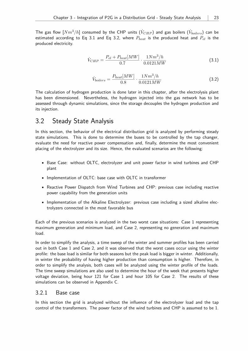
Chapter 3 - Integration of P2G in a Distribution Grid - Steady State Analysis 23
The gas flow [Nm3/h] consumed by the CHP units (VCHP ) and gas boilers (Vboilers) can beestimated according to Eq 3.1 and Eq 3.2, where Pheat is the produced heat and Pel is theproduced electricity.
VCHP = Pel + Pheat[MW ]0.7 · 1Nm3/h
0.0121MW(3.1)
Vboilers = Pheat[MW ]0.8 · 1Nm3/h
0.0121MW(3.2)
The calculation of hydrogen production is done later in this chapter, after the electrolysis planthas been dimensioned. Nevertheless, the hydrogen injected into the gas network has to beassessed through dynamic simulations, since the storage decouples the hydrogen production andits injection.
3.2 Steady State AnalysisIn this section, the behavior of the electrical distribution grid is analyzed by performing steadystate simulations. This is done to determine the buses to be controlled by the tap changer,evaluate the need for reactive power compensation and, finally, determine the most convenientplacing of the electrolyzer and its size. Hence, the evaluated scenarios are the following:
• Base Case: without OLTC, electrolyzer and unit power factor in wind turbines and CHPplant
• Implementation of OLTC: base case with OLTC in transformer
• Reactive Power Dispatch from Wind Turbines and CHP: previous case including reactivepower capability from the generation units
• Implementation of the Alkaline Electrolyzer: previous case including a sized alkaline elec-trolyzers connected in the most favorable bus
Each of the previous scenarios is analyzed in the two worst case situations: Case 1 representingmaximum generation and minimum load, and Case 2, representing no generation and maximumload.
In order to simplify the analysis, a time sweep of the winter and summer profiles has been carriedout in both Case 1 and Case 2, and it was observed that the worst cases occur using the winterprofile: the base load is similar for both seasons but the peak load is bigger in winter. Additionally,in winter the probability of having higher production than consumption is higher. Therefore, inorder to simplify the analysis, both cases will be analyzed using the winter profile of the loads.The time sweep simulations are also used to determine the hour of the week that presents highervoltage deviation, being hour 121 for Case 1 and hour 105 for Case 2. The results of thesesimulations can be observed in Appendix C.
3.2.1 Base caseIn this section the grid is analyzed without the influence of the electrolyzer load and the tapcontrol of the transformers. The power factor of the wind turbines and CHP is assumed to be 1.
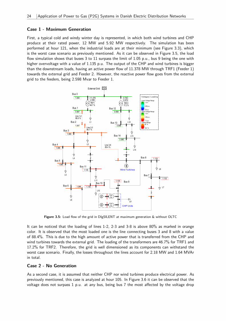
24 Application of Power to Gas (P2G) Systems in Danish Electric Distribution Networks
Case 1 - Maximum Generation
First, a typical cold and windy winter day is represented, in which both wind turbines and CHPproduce at their rated power, 12 MW and 5.92 MW respectively. The simulation has beenperformed at hour 121, when the industrial loads are at their minimum (see Figure 3.3), whichis the worst case scenario as previously mentioned. As it can be observed in Figure 3.5, the loadflow simulation shows that buses 3 to 11 surpass the limit of 1.05 p.u., bus 9 being the one withhigher overvoltage with a value of 1.135 p.u. The output of the CHP and wind turbines is biggerthan the downstream loads, having an active power flow of 11.378 MW through TRF1 (Feeder 1)towards the external grid and Feeder 2. However, the reactive power flow goes from the externalgrid to the feeders, being 2.598 Mvar to Feeder 1.
Voltages / Loading
Lower Voltage Range1. p.u....0.95 p.u....0.9 p.u.
Upper Voltage Range1. p.u....1.05 p.u....1.1 p.u.
Loading Range80. %...100. %
Wind Turbines
CHP Units
Te
rmin
al(
7)
Te
rmin
al(
6)
Terminal(5)
Terminal(4)
Terminal(3)
Terminal(2)
Terminal(1)
Terminal
Bus 91.135
Bus 14
0.995
Bus 130.998
Bus 6 1.089
Bus 71.133
Bus 8 1.133
Bus 101.135
Bus 111.135
Bus 5
1.089
Bus 2
1.047
Bus 41.089
Bus 31.089
Bus 120.999
Bus 1
0.997
Bus 0
1.000
Sta
tic
Ge
..0
.0%
SG~
Syn
chro
no
..2
9.5
%
SG~
Syn
chro
no
..2
9.5
%2-Winding..
65.0 %
2-Winding..65.0 %
Line 9-100.8 %
Lin
ec-
80
.0%
Static Ge..60.0 %
L9
L4
Bre
ake
r/S
..0
.0%
Lin
e1
4-c
0.0
%
Bre
ake
r/S
..0
.0%
Line 6-b0.0 %
Lin
eb
-70
.0%
Lin
ea
-11
0.0
%
Lin
e4
-a0
.0%
Bre
ake
r/S
wit
ch0
.0%
Line 3-888.4 %
L8
Line 8-928.2 %
L10
L14
Lin
e1
3-1
44
.0%
L13
Line 12-134.1 %
L12
Lin
e5
-60
.5%
L6
L7
Lin
e7
-80
.7%
Lin
e1
0-1
10
.2%
L11
L5L
ine
4-5
1.3
%
Line 1-286.6 %
L1
Line 2-386.7 %
Lin
e3
-41
.5%
L3
TRF217.2 %
4.1820.979
TRF146.7 %
-11.3782.598
External Grid
DIgSILENT
Figure 3.5: Load flow of the grid in DIgSILENT at maximum generation & without OLTC
It can be noticed that the loading of lines 1-2, 2-3 and 3-8 is above 80% as marked in orangecolor. It is observed that the most loaded one is the line connecting buses 3 and 8 with a valueof 88.4%. This is due to the high amount of active power that is transferred from the CHP andwind turbines towards the external grid. The loading of the transformers are 46.7% for TRF1 and17.2% for TRF2. Therefore, the grid is well dimensioned as its components can withstand theworst case scenario. Finally, the losses throughout the lines account for 2.18 MW and 1.64 MVArin total.
Case 2 - No Generation
As a second case, it is assumed that neither CHP nor wind turbines produce electrical power. Aspreviously mentioned, this case is analyzed at hour 105. In Figure 3.6 it can be observed that thevoltage does not surpass 1 p.u. at any bus, being bus 7 the most affected by the voltage drop
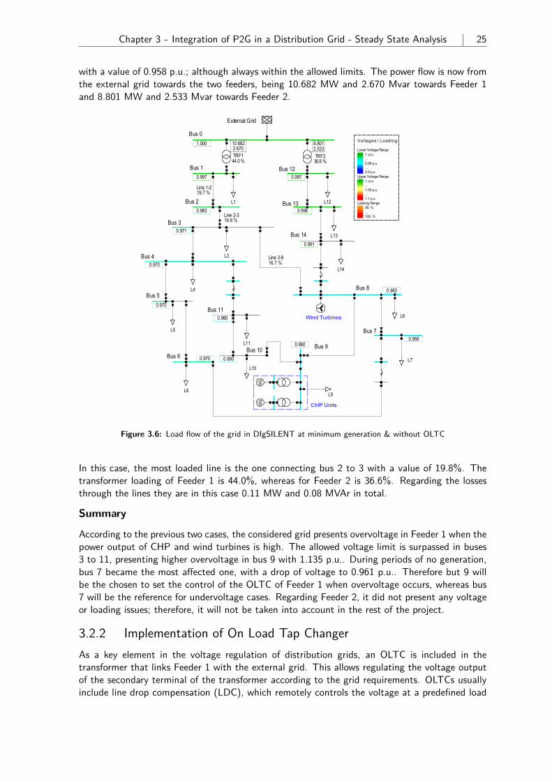
Chapter 3 - Integration of P2G in a Distribution Grid - Steady State Analysis 25
with a value of 0.958 p.u.; although always within the allowed limits. The power flow is now fromthe external grid towards the two feeders, being 10.682 MW and 2.670 Mvar towards Feeder 1and 8.801 MW and 2.533 Mvar towards Feeder 2.
Voltages / Loading
Lower Voltage Range1. p.u....0.95 p.u....0.9 p.u.
Upper Voltage Range1. p.u....1.05 p.u....1.1 p.u.
Loading Range80. %...100. %
Wind Turbines
CHP Units
Te
rmin
al(
7)
Te
rmin
al(
6)
Terminal(5)
Terminal(4)
Terminal(3)
Terminal(2)
Terminal(1)
Terminal
Bus 90.960
Bus 14
0.991
Bus 130.996
Bus 6 0.970
Bus 70.958
Bus 8 0.960
Bus 100.960
Bus 110.960
Bus 5
0.970
Bus 2
0.983
Bus 40.970
Bus 30.971
Bus 120.997
Bus 1
0.997
Bus 0
1.000
Sta
tic
Ge
..0
.0%
SG~
Syn
chro
no
..0
.0%
SG~
Syn
chro
no
..0
.0%
2-Winding..0.0 %
2-Winding..0.0 %
Line 9-101.3 %
Lin
ec-
80
.0%
Static Ge..0.0 %
L9
L4
Bre
ake
r/S
..0
.0%
Lin
e1
4-c
0.0
%
Bre
ake
r/S
..0
.0%
Line 6-b0.0 %
Lin
eb
-70
.0%
Lin
ea
-11
0.0
%
Lin
e4
-a0
.0%
Bre
ake
r/S
wit
ch0
.0%
Line 3-816.7 %
L8
Line 8-910.3 %
L10
L14
Lin
e1
3-1
47
.0%
L13
Line 12-138.3 %
L12
Lin
e5
-60
.6%
L6
L7
Lin
e7
-86
.1%
Lin
e1
0-1
10
.3%
L11
L5
Lin
e4
-51
.8%
Line 1-219.7 %
L1
Line 2-319.8 %
Lin
e3
-42
.0%
L3
TRF236.6 %
8.8012.533
TRF144.0 %
10.6822.670
External Grid
DIgSILENT
Figure 3.6: Load flow of the grid in DIgSILENT at minimum generation & without OLTC
In this case, the most loaded line is the one connecting bus 2 to 3 with a value of 19.8%. Thetransformer loading of Feeder 1 is 44.0%, whereas for Feeder 2 is 36.6%. Regarding the lossesthrough the lines they are in this case 0.11 MW and 0.08 MVAr in total.
Summary
According to the previous two cases, the considered grid presents overvoltage in Feeder 1 when thepower output of CHP and wind turbines is high. The allowed voltage limit is surpassed in buses3 to 11, presenting higher overvoltage in bus 9 with 1.135 p.u.. During periods of no generation,bus 7 became the most affected one, with a drop of voltage to 0.961 p.u.. Therefore but 9 willbe the chosen to set the control of the OLTC of Feeder 1 when overvoltage occurs, whereas bus7 will be the reference for undervoltage cases. Regarding Feeder 2, it did not present any voltageor loading issues; therefore, it will not be taken into account in the rest of the project.
3.2.2 Implementation of On Load Tap ChangerAs a key element in the voltage regulation of distribution grids, an OLTC is included in thetransformer that links Feeder 1 with the external grid. This allows regulating the voltage outputof the secondary terminal of the transformer according to the grid requirements. OLTCs usuallyinclude line drop compensation (LDC), which remotely controls the voltage at a predefined load
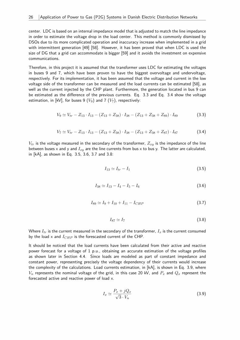
26 Application of Power to Gas (P2G) Systems in Danish Electric Distribution Networks
center. LDC is based on an internal impedance model that is adjusted to match the line impedancein order to estimate the voltage drop in the load center. This method is commonly dismissed byDSOs due to its more complicated operation and inaccuracy increase when implemented in a gridwith intermittent generation [49] [58]. However, it has been proved that when LDC is used thesize of DG that a grid can accommodate is bigger [59] and it avoids the investment on expensivecommunications.
Therefore, in this project it is assumed that the transformer uses LDC for estimating the voltagesin buses 9 and 7, which have been proven to have the biggest overvoltage and undervoltage,respectively. For its implementation, it has been assumed that the voltage and current in the lowvoltage side of the transformer can be measured and the load currents can be estimated [58], aswell as the current injected by the CHP plant. Furthermore, the generation located in bus 9 canbe estimated as the difference of the previous currents. Eq. 3.3 and Eq. 3.4 show the voltageestimation, in [kV], for buses 9 (V9) and 7 (V7), respectively:
V9 ' Vtr − Z13 · I13 − (Z13 + Z38) · I38 − (Z13 + Z38 + Z89) · I89 (3.3)
V7 ' Vtr − Z13 · I13 − (Z13 + Z38) · I38 − (Z13 + Z38 + Z87) · I87 (3.4)
Vtr is the voltage measured in the secondary of the transformer, Zxy is the impedance of the linebetween buses x and y and Ixy are the line currents from bus x to bus y. The latter are calculated,in [kA], as shown in Eq. 3.5, 3.6, 3.7 and 3.8:
I13 ' Itr − I1 (3.5)
I38 ' I13 − I4 − I5 − I6 (3.6)
I89 ' I9 + I10 + I11 − ICHP (3.7)
I87 ' I7 (3.8)
Where Itr is the current measured in the secondary of the transformer, Ix is the current consumedby the load x and ICHP is the forescasted current of the CHP.
It should be noticed that the load currents have been calculated from their active and reactivepower forecast for a voltage of 1 p.u., obtaining an accurate estimation of the voltage profilesas shown later in Section 4.4. Since loads are modeled as part of constant impedance andconstant power, representing precisely the voltage dependency of their currents would increasethe complexity of the calculations. Load currents estimation, in [kA], is shown in Eq. 3.9, whereVn represents the nominal voltage of the grid, in this case 20 kV, and Px and Qx represent theforecasted active and reactive power of load x.
Ix 'Px + jQx√
3 · Vn(3.9)
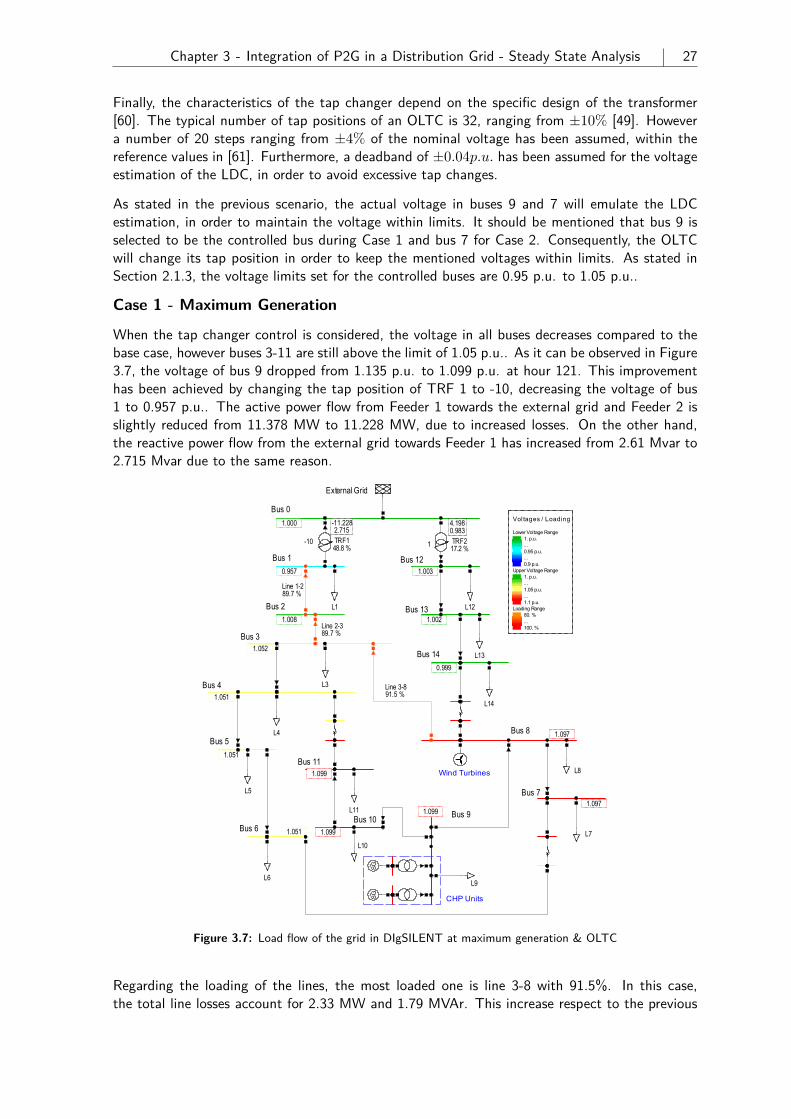
Chapter 3 - Integration of P2G in a Distribution Grid - Steady State Analysis 27
Finally, the characteristics of the tap changer depend on the specific design of the transformer[60]. The typical number of tap positions of an OLTC is 32, ranging from ±10% [49]. Howevera number of 20 steps ranging from ±4% of the nominal voltage has been assumed, within thereference values in [61]. Furthermore, a deadband of ±0.04p.u. has been assumed for the voltageestimation of the LDC, in order to avoid excessive tap changes.
As stated in the previous scenario, the actual voltage in buses 9 and 7 will emulate the LDCestimation, in order to maintain the voltage within limits. It should be mentioned that bus 9 isselected to be the controlled bus during Case 1 and bus 7 for Case 2. Consequently, the OLTCwill change its tap position in order to keep the mentioned voltages within limits. As stated inSection 2.1.3, the voltage limits set for the controlled buses are 0.95 p.u. to 1.05 p.u..
Case 1 - Maximum Generation
When the tap changer control is considered, the voltage in all buses decreases compared to thebase case, however buses 3-11 are still above the limit of 1.05 p.u.. As it can be observed in Figure3.7, the voltage of bus 9 dropped from 1.135 p.u. to 1.099 p.u. at hour 121. This improvementhas been achieved by changing the tap position of TRF 1 to -10, decreasing the voltage of bus1 to 0.957 p.u.. The active power flow from Feeder 1 towards the external grid and Feeder 2 isslightly reduced from 11.378 MW to 11.228 MW, due to increased losses. On the other hand,the reactive power flow from the external grid towards Feeder 1 has increased from 2.61 Mvar to2.715 Mvar due to the same reason.
Voltages / Loading
Lower Voltage Range1. p.u....0.95 p.u....0.9 p.u.
Upper Voltage Range1. p.u....1.05 p.u....1.1 p.u.
Loading Range80. %...100. %
Wind Turbines
CHP Units
Te
rmin
al(
7)
Te
rmin
al(
6)
Terminal(5)
Terminal(4)
Terminal(3)
Terminal(2)
Terminal(1)
Terminal
Bus 91.099
Bus 14
0.999
Bus 131.002
Bus 6 1.051
Bus 71.097
Bus 8 1.097
Bus 101.099
Bus 111.099
Bus 5
1.051
Bus 2
1.008
Bus 41.051
Bus 31.052
Bus 121.003
Bus 1
0.957
Bus 0
1.000
Sta
tic
Ge
..0
.0%
SG~
Syn
chro
no
..2
9.6
%
SG~
Syn
chro
no
..2
9.6
%
2-Winding..67.4 %
2-Winding..67.4 %
Line 9-100.8 %
Lin
ec-
80
.0%
Static Ge..60.0 %
L9
L4
Bre
ake
r/S
..0
.0%
Lin
e1
4-c
0.0
%
Bre
ake
r/S
..0
.0%
Line 6-b0.0 %
Lin
eb
-70
.0%
Lin
ea
-11
0.0
%
Lin
e4
-a0
.0%
Bre
ake
r/S
wit
ch0
.0%
Line 3-891.5 %
L8
Line 8-929.3 %
L10
L14
Lin
e1
3-1
44
.0%
L13
Line 12-134.1 %
L12
Lin
e5
-60
.4%
L6
L7
Lin
e7
-80
.7%
Lin
e1
0-1
10
.2%
L11
L5
Lin
e4
-51
.3%
Line 1-289.7 %
L1
Line 2-389.7 %
Lin
e3
-41
.5%
L3
TRF217.2 %
4.1980.983
1TRF148.8 %
-11.2282.715
-10
External Grid
DIgSILENT
Figure 3.7: Load flow of the grid in DIgSILENT at maximum generation & OLTC
Regarding the loading of the lines, the most loaded one is line 3-8 with 91.5%. In this case,the total line losses account for 2.33 MW and 1.79 MVAr. This increase respect to the previous
28 Application of Power to Gas (P2G) Systems in Danish Electric Distribution Networks
scenario is due to higher current through the lines, as the generation and an important part ofthe loads are modeled as constant power.
Case 2 - No Generation
When the wind turbines and CHP do not produce any power, the tap position of TRF 1 changesto 3, increasing the voltage of the secondary by 1.2%. As in the previous section, the load flowhas been performed at hour 105, as it is the most critical. The voltage at bus 7, the mostsusceptible to voltage drops as explained in the previous scenario, increased from 0.958 p.u. to0.971 p.u.. Furthermore, the power flow from the external grid towards Feeder 1 increased from10.682 MW to 10.771 MW and 2.67 Mvar to 2.685 Mvar due to the higher consumption of thevoltage dependence loads. This can be observed in Figure 3.8.
Voltages / Loading
Lower Voltage Range1. p.u....0.95 p.u....0.9 p.u.
Upper Voltage Range1. p.u....1.05 p.u....1.1 p.u.
Loading Range80. %...100. %
Wind Turbines
CHP Units
Te
rmin
al(
7)
Te
rmin
al(
6)
Terminal(5)
Terminal(4)
Terminal(3)
Terminal(2)
Terminal(1)
Terminal
Bus 90.972
Bus 14
0.995
Bus 131.000
Bus 6 0.982
Bus 70.971
Bus 8 0.973
Bus 100.972
Bus 110.972
Bus 5
0.982
Bus 2
0.995
Bus 40.983
Bus 30.983
Bus 121.001
Bus 1
1.009
Bus 0
1.000
Sta
tic
Ge
..0
.0%
SG~
Syn
chro
no
..0
.0%
SG~
Syn
chro
no
..0
.0%
2-Winding..0.0 %
2-Winding..0.0 %
Line 9-101.3 %
Lin
ec-
80
.0%
Static Ge..0.0 %
L9
L4
Bre
ake
r/S
..0
.0%
Lin
e1
4-c
0.0
%
Bre
ake
r/S
..0
.0%
Line 6-b0.0 %
Lin
eb
-70
.0%
Lin
ea
-11
0.0
%
Lin
e4
-a0
.0%
Bre
ake
r/S
wit
ch0
.0%
Line 3-816.5 %
L8
Line 8-910.2 %
L10
L14
Lin
e1
3-1
47
.0%
L13
Line 12-138.3 %
L12
Lin
e5
-60
.6%
L6
L7
Lin
e7
-86
.1%
Lin
e1
0-1
10
.3%
L11
L5
Lin
e4
-51
.8%
Line 1-219.5 %
L1
Line 2-319.6 %
Lin
e3
-42
.0%
L3
TRF236.8 %
8.8332.543
1TRF144.4 %
10.7712.685
3
External Grid
DIgSILENT
Figure 3.8: Load flow of the grid in DIgSILENT at no generation & OLTC
As in the previous scenario, the most loaded line is the one connecting bus 2 to 3 with a value of19.6%. Regarding the line losses, the total value is 0.11 MW and 0.08 MVAr.
Summary
It can be concluded that the tap changer control presents a significant improvement in the busesof Feeder 1, although the overvoltage issues persist. Regarding the loading of the lines in Case 1,it has been observed that it was higher than in the previous scenario, although remaining below100%. This increase was due to the voltage reduction while transporting the same apparentpower. The improvement in voltage is summarized in Table 3.5.
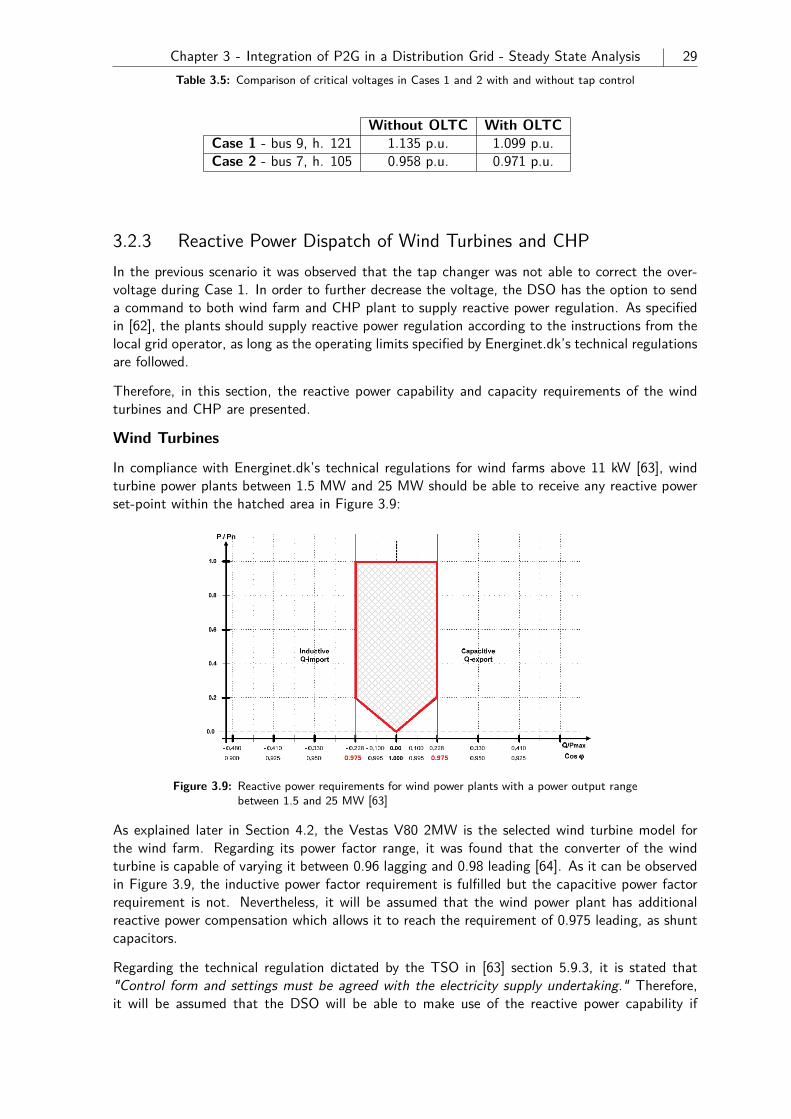
Chapter 3 - Integration of P2G in a Distribution Grid - Steady State Analysis 29Table 3.5: Comparison of critical voltages in Cases 1 and 2 with and without tap control
Without OLTC With OLTCCase 1 - bus 9, h. 121 1.135 p.u. 1.099 p.u.Case 2 - bus 7, h. 105 0.958 p.u. 0.971 p.u.
3.2.3 Reactive Power Dispatch of Wind Turbines and CHPIn the previous scenario it was observed that the tap changer was not able to correct the over-voltage during Case 1. In order to further decrease the voltage, the DSO has the option to senda command to both wind farm and CHP plant to supply reactive power regulation. As specifiedin [62], the plants should supply reactive power regulation according to the instructions from thelocal grid operator, as long as the operating limits specified by Energinet.dk’s technical regulationsare followed.
Therefore, in this section, the reactive power capability and capacity requirements of the windturbines and CHP are presented.
Wind Turbines
In compliance with Energinet.dk’s technical regulations for wind farms above 11 kW [63], windturbine power plants between 1.5 MW and 25 MW should be able to receive any reactive powerset-point within the hatched area in Figure 3.9:
Figure 3.9: Reactive power requirements for wind power plants with a power output rangebetween 1.5 and 25 MW [63]
As explained later in Section 4.2, the Vestas V80 2MW is the selected wind turbine model forthe wind farm. Regarding its power factor range, it was found that the converter of the windturbine is capable of varying it between 0.96 lagging and 0.98 leading [64]. As it can be observedin Figure 3.9, the inductive power factor requirement is fulfilled but the capacitive power factorrequirement is not. Nevertheless, it will be assumed that the wind power plant has additionalreactive power compensation which allows it to reach the requirement of 0.975 leading, as shuntcapacitors.
Regarding the technical regulation dictated by the TSO in [63] section 5.9.3, it is stated that"Control form and settings must be agreed with the electricity supply undertaking." Therefore,it will be assumed that the DSO will be able to make use of the reactive power capability if
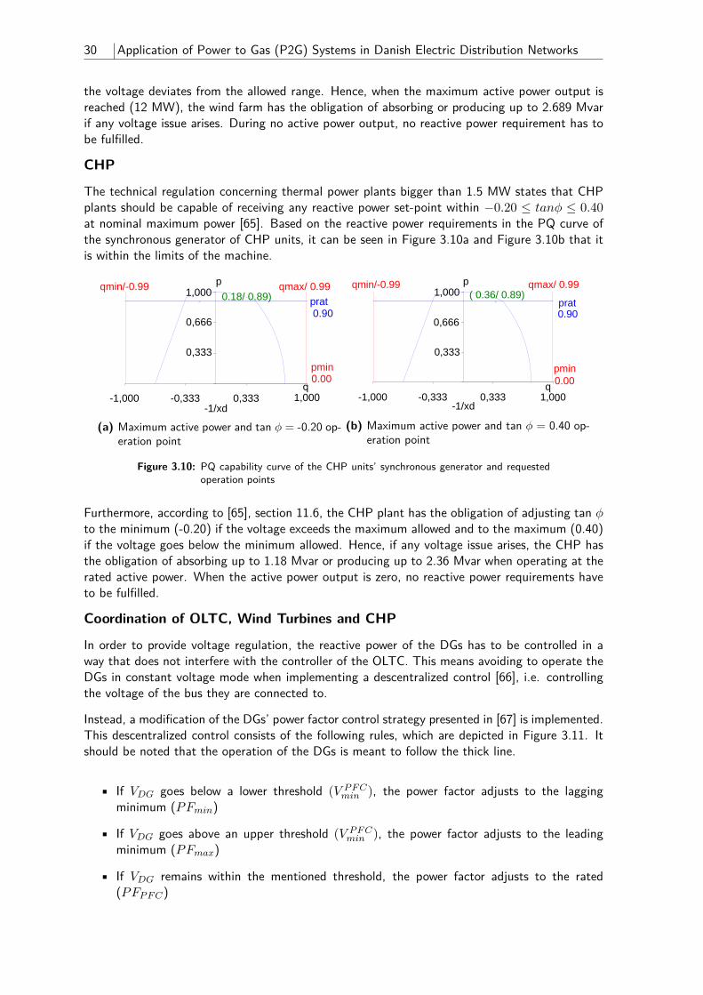
30 Application of Power to Gas (P2G) Systems in Danish Electric Distribution Networks
the voltage deviates from the allowed range. Hence, when the maximum active power output isreached (12 MW), the wind farm has the obligation of absorbing or producing up to 2.689 Mvarif any voltage issue arises. During no active power output, no reactive power requirement has tobe fulfilled.
CHP
The technical regulation concerning thermal power plants bigger than 1.5 MW states that CHPplants should be capable of receiving any reactive power set-point within −0.20 ≤ tanφ ≤ 0.40at nominal maximum power [65]. Based on the reactive power requirements in the PQ curve ofthe synchronous generator of CHP units, it can be seen in Figure 3.10a and Figure 3.10b that itis within the limits of the machine.
q0,333-0,333-1,000
1,000
0,666
0,333 pmin
pqmin/-0.99 qmax/ 0.990.18/ 0.89) prat
0.90
0.00
-1/xd
DIg
SIL
EN
T
1,0 00
(a) Maximum active power and tan φ = -0.20 op-eration point
1,0 000,333-0,333-1,000
1,000
0,666
0,333
pmin
pqmin/-0.99 qmax/ 0.99
prat 0.90
0.00
-1/xd
DIg
SIL
EN
T
q
( 0.36/ 0.89)
(b) Maximum active power and tan φ = 0.40 op-eration point
Figure 3.10: PQ capability curve of the CHP units’ synchronous generator and requestedoperation points
Furthermore, according to [65], section 11.6, the CHP plant has the obligation of adjusting tan φto the minimum (-0.20) if the voltage exceeds the maximum allowed and to the maximum (0.40)if the voltage goes below the minimum allowed. Hence, if any voltage issue arises, the CHP hasthe obligation of absorbing up to 1.18 Mvar or producing up to 2.36 Mvar when operating at therated active power. When the active power output is zero, no reactive power requirements haveto be fulfilled.
Coordination of OLTC, Wind Turbines and CHP
In order to provide voltage regulation, the reactive power of the DGs has to be controlled in away that does not interfere with the controller of the OLTC. This means avoiding to operate theDGs in constant voltage mode when implementing a descentralized control [66], i.e. controllingthe voltage of the bus they are connected to.
Instead, a modification of the DGs’ power factor control strategy presented in [67] is implemented.This descentralized control consists of the following rules, which are depicted in Figure 3.11. Itshould be noted that the operation of the DGs is meant to follow the thick line.
• If VDG goes below a lower threshold (V PFCmin ), the power factor adjusts to the lagging
minimum (PFmin)
• If VDG goes above an upper threshold (V PFCmin ), the power factor adjusts to the leading
minimum (PFmax)
• If VDG remains within the mentioned threshold, the power factor adjusts to the rated(PFPFC)
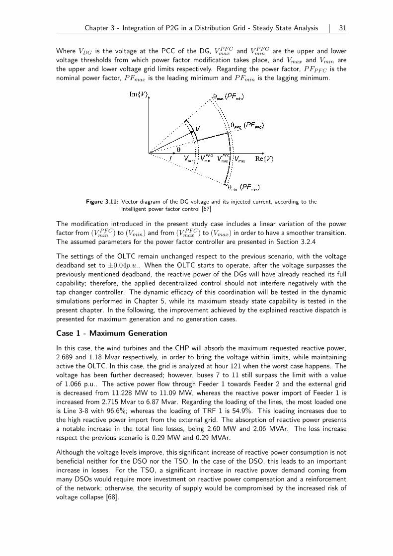
Chapter 3 - Integration of P2G in a Distribution Grid - Steady State Analysis 31
Where VDG is the voltage at the PCC of the DG, V PFCmax and V PFC
min are the upper and lowervoltage thresholds from which power factor modification takes place, and Vmax and Vmin arethe upper and lower voltage grid limits respectively. Regarding the power factor, PFPFC is thenominal power factor, PFmax is the leading minimum and PFmin is the lagging minimum.
VOVOS et al.: CENTRALIZED AND DISTRIBUTED VOLTAGE CONTROL 477
Fig. 1. Simple two-bus system.
the DG bus toward the bulk supply point (BSP). Any fluctuationin real power brings about a proportional fluctuation of voltage.This is particularly evident in cases of weak networks where theline resistance is high relative to its reactance. In power factorcontrol mode, the ratio is maintained constant, so fol-lows any variation of , tending to augment the voltage varia-tion. It is for these reasons that voltage rise is regarded as one ofthe major impacts of, and constraints on, the connection of newDGs on the network, particularly in rural areas [1].
In (1), if was allowed to compensate for the feeder voltagerise or drop created by by adjusting in the opposite direction(with ), then voltage could be maintained within limits al-lowing greater active power export. For voltage rise, this wouldbe achieved by defining a more leading power factor at whichthe generator is to be controlled. Power factor settings couldbe specified so that DG operates at lagging power factor toexport reactive power during high demand periods while im-porting during low demand. While this appears to be a rela-tively simple approach, it would require analysis to ensure thatvoltage is maintained appropriately under all normal operationcases and may require a degree of central coordination.
B. Voltage Regulation or Power Factor Control
DNOs have hitherto been reluctant to allow any operation byindependent generators, which could potentially disrupt the pas-sive role of the distribution network to supply demand. Specif-ically, distributed generators are not permitted to perform au-tomatic voltage regulation (AVR), an inherent feature of syn-chronous generators to regulate the terminal bus voltage by ad-justing their reactive power output, as it may destabilize theautomatic OLTCs of some distribution transformers. A furtherreason for the avoidance of AVR in most distributed generationapplications is that should a small generator with AVR con-trol attempt to correct for voltage drops, it has to inject greatamounts of reactive power in order to raise the bus voltage. Thismay result in high field currents and overheating for the gen-erator, triggering the excitation limit or over-current protectionand disconnecting the generator from the network.
For the above reasons, most distributed generators have beenrequired by the DNOs to operate in power factor control mode.PFC is less disruptive for network voltage control devices suchas OLTCs and results in much lower field currents brought aboutby voltage drops under AVR control, thereby reducing thermalstresses on the generator [9].
C. Alternative Voltage Control
1) “Intelligent” Distributed Voltage/Power Factor Control:Kiprakis and Wallace [5] proposed a voltage control method
Fig. 2. Vector diagram of the generator voltage and current showing the re-sponse of the “intelligent” distributed controller.
for DGs, which assumes a more flexible attitude from DNOsconcerning the voltage control by DGs. The authors’ targetwas to develop a voltage control method capable of keepingthe DGs online during light or heavy demand conditions bycombining the advantages of AVR and PFC. The method wastermed automatic voltage/power factor control (AVPFC), andits steady-state response has the effect of relaxing power factorwhen voltage approaches the statutory limits. Its operation isdepicted in the vector diagram of Fig. 2.
The operating point of the generator (tip of vector ) alwaysmoves along the thick, dashed line. When voltage approachesthe statutory limits, or , the PFC is deactivated and theDG adjusts the production of reactive power to support voltage.The generator decreases the ratio when voltage drops tothe lower threshold, , while it increases the ratiowhen voltage reaches the upper threshold . Obviously, inaltering the ratio, the power factor is also being changed:it must be restricted between the minimum and max-imum operating power factors.
The major advantage of this approach is that it does not re-quire knowledge of the distribution network as a whole, relyingpurely on the voltage signals at its own terminals. As such, theapproach would not require extensive deployment of sensorsand communications equipment and the “intelligence” can beembedded within the DG control system. However, the con-trollers would need to be set up such that they did not conflictwith others, e.g., by causing hunting.
2) Centralized Voltage Control: Theoretically, voltage con-trol of the distribution network can be achieved centrally, in asimilar manner to the transmission system through dispatch ofactive and reactive power from distributed generators and othernetwork elements.
Such an active management scheme would consist of a distri-bution management system controller accepting voltage, powerflow, and equipment status measurements at selected locationsin the distribution network. The controller would then use stateestimation to estimate network power flow and voltage profilesbefore dispatching plant according to economic dispatch fromOPF [4] or a rule-based method.
The downsides to the approach include the necessary invest-ment in sensors, communications, and dedicated controllers aswell as the balance required to ensure adequate accuracy of thestate estimator.
Figure 3.11: Vector diagram of the DG voltage and its injected current, according to theintelligent power factor control [67]
The modification introduced in the present study case includes a linear variation of the powerfactor from (V PFC
min ) to (Vmin) and from (V PFCmax ) to (Vmax) in order to have a smoother transition.
The assumed parameters for the power factor controller are presented in Section 3.2.4
The settings of the OLTC remain unchanged respect to the previous scenario, with the voltagedeadband set to ±0.04p.u.. When the OLTC starts to operate, after the voltage surpasses thepreviously mentioned deadband, the reactive power of the DGs will have already reached its fullcapability; therefore, the applied decentralized control should not interfere negatively with thetap changer controller. The dynamic efficacy of this coordination will be tested in the dynamicsimulations performed in Chapter 5, while its maximum steady state capability is tested in thepresent chapter. In the following, the improvement achieved by the explained reactive dispatch ispresented for maximum generation and no generation cases.
Case 1 - Maximum Generation
In this case, the wind turbines and the CHP will absorb the maximum requested reactive power,2.689 and 1.18 Mvar respectively, in order to bring the voltage within limits, while maintainingactive the OLTC. In this case, the grid is analyzed at hour 121 when the worst case happens. Thevoltage has been further decreased; however, buses 7 to 11 still surpass the limit with a valueof 1.066 p.u.. The active power flow through Feeder 1 towards Feeder 2 and the external gridis decreased from 11.228 MW to 11.09 MW, whereas the reactive power import of Feeder 1 isincreased from 2.715 Mvar to 6.87 Mvar. Regarding the loading of the lines, the most loaded oneis Line 3-8 with 96.6%; whereas the loading of TRF 1 is 54.9%. This loading increases due tothe high reactive power import from the external grid. The absorption of reactive power presentsa notable increase in the total line losses, being 2.60 MW and 2.06 MVAr. The loss increaserespect the previous scenario is 0.29 MW and 0.29 MVAr.
Although the voltage levels improve, this significant increase of reactive power consumption is notbeneficial neither for the DSO nor the TSO. In the case of the DSO, this leads to an importantincrease in losses. For the TSO, a significant increase in reactive power demand coming frommany DSOs would require more investment on reactive power compensation and a reinforcementof the network; otherwise, the security of supply would be compromised by the increased risk ofvoltage collapse [68].
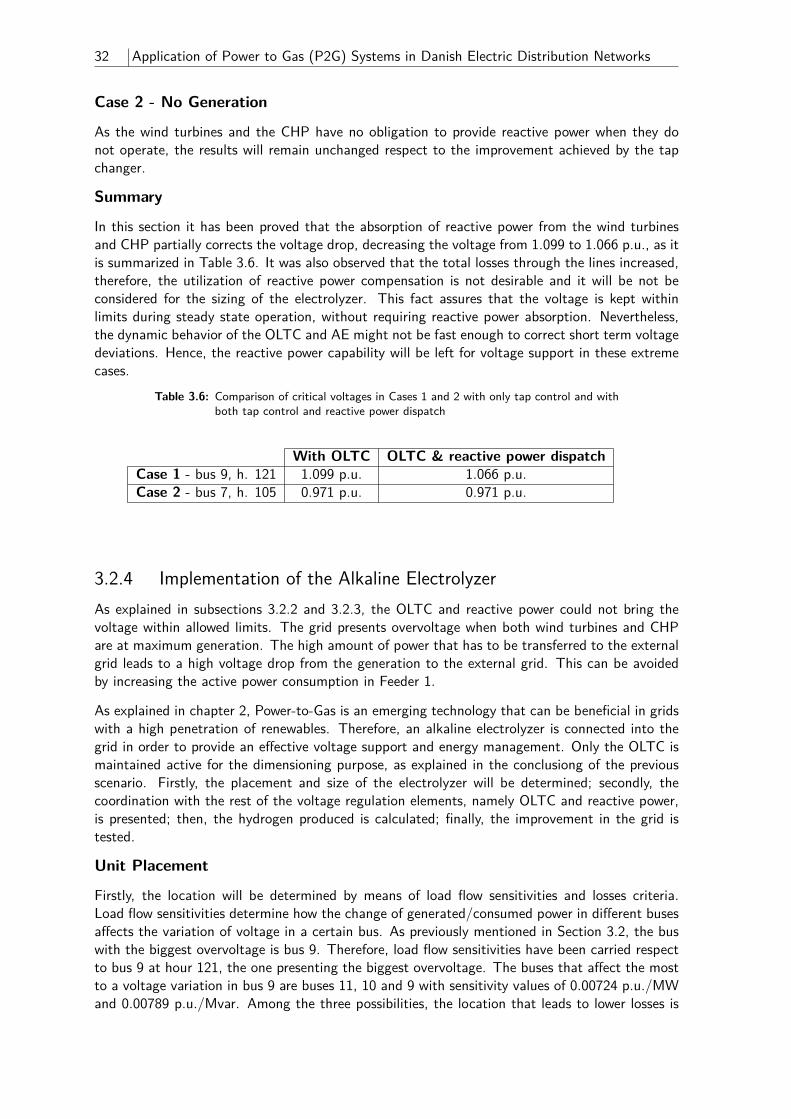
32 Application of Power to Gas (P2G) Systems in Danish Electric Distribution Networks
Case 2 - No Generation
As the wind turbines and the CHP have no obligation to provide reactive power when they donot operate, the results will remain unchanged respect to the improvement achieved by the tapchanger.
Summary
In this section it has been proved that the absorption of reactive power from the wind turbinesand CHP partially corrects the voltage drop, decreasing the voltage from 1.099 to 1.066 p.u., as itis summarized in Table 3.6. It was also observed that the total losses through the lines increased,therefore, the utilization of reactive power compensation is not desirable and it will be not beconsidered for the sizing of the electrolyzer. This fact assures that the voltage is kept withinlimits during steady state operation, without requiring reactive power absorption. Nevertheless,the dynamic behavior of the OLTC and AE might not be fast enough to correct short term voltagedeviations. Hence, the reactive power capability will be left for voltage support in these extremecases.
Table 3.6: Comparison of critical voltages in Cases 1 and 2 with only tap control and withboth tap control and reactive power dispatch
With OLTC OLTC & reactive power dispatchCase 1 - bus 9, h. 121 1.099 p.u. 1.066 p.u.Case 2 - bus 7, h. 105 0.971 p.u. 0.971 p.u.
3.2.4 Implementation of the Alkaline ElectrolyzerAs explained in subsections 3.2.2 and 3.2.3, the OLTC and reactive power could not bring thevoltage within allowed limits. The grid presents overvoltage when both wind turbines and CHPare at maximum generation. The high amount of power that has to be transferred to the externalgrid leads to a high voltage drop from the generation to the external grid. This can be avoidedby increasing the active power consumption in Feeder 1.
As explained in chapter 2, Power-to-Gas is an emerging technology that can be beneficial in gridswith a high penetration of renewables. Therefore, an alkaline electrolyzer is connected into thegrid in order to provide an effective voltage support and energy management. Only the OLTC ismaintained active for the dimensioning purpose, as explained in the conclusiong of the previousscenario. Firstly, the placement and size of the electrolyzer will be determined; secondly, thecoordination with the rest of the voltage regulation elements, namely OLTC and reactive power,is presented; then, the hydrogen produced is calculated; finally, the improvement in the grid istested.
Unit Placement
Firstly, the location will be determined by means of load flow sensitivities and losses criteria.Load flow sensitivities determine how the change of generated/consumed power in different busesaffects the variation of voltage in a certain bus. As previously mentioned in Section 3.2, the buswith the biggest overvoltage is bus 9. Therefore, load flow sensitivities have been carried respectto bus 9 at hour 121, the one presenting the biggest overvoltage. The buses that affect the mostto a voltage variation in bus 9 are buses 11, 10 and 9 with sensitivity values of 0.00724 p.u./MWand 0.00789 p.u./Mvar. Among the three possibilities, the location that leads to lower losses is
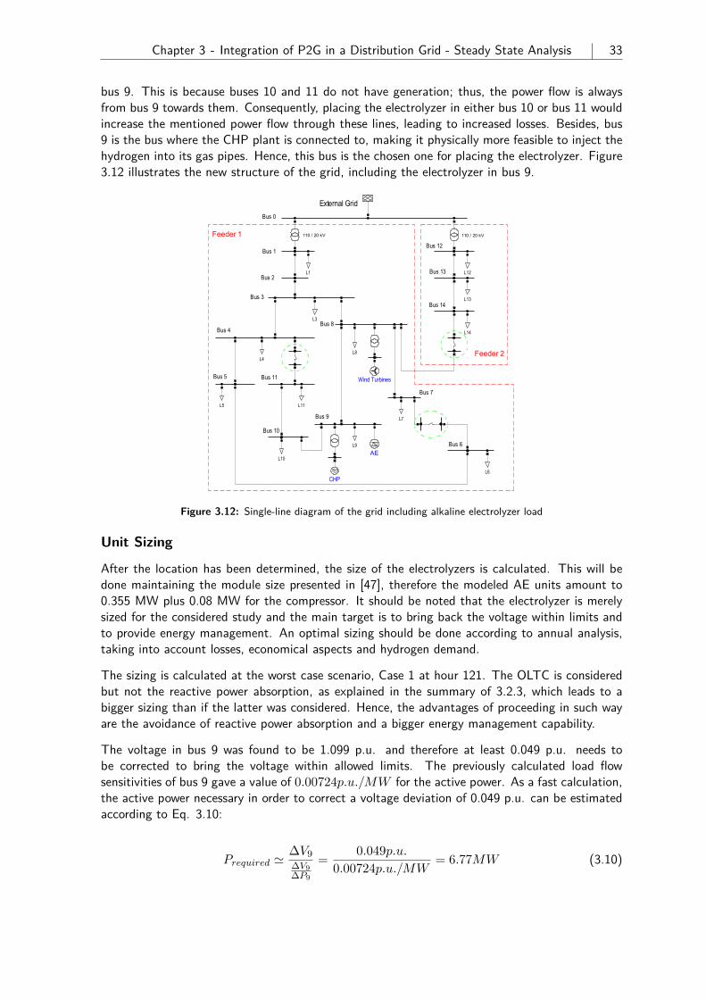
Chapter 3 - Integration of P2G in a Distribution Grid - Steady State Analysis 33
bus 9. This is because buses 10 and 11 do not have generation; thus, the power flow is alwaysfrom bus 9 towards them. Consequently, placing the electrolyzer in either bus 10 or bus 11 wouldincrease the mentioned power flow through these lines, leading to increased losses. Besides, bus9 is the bus where the CHP plant is connected to, making it physically more feasible to inject thehydrogen into its gas pipes. Hence, this bus is the chosen one for placing the electrolyzer. Figure3.12 illustrates the new structure of the grid, including the electrolyzer in bus 9.
AE
Feeder 1 110 / 20 kV110 / 20 kV
Feeder 2
Bus 12
Bus 0
Bus 1
Bus 3
Terminal(4)
Terminal(5)
Bus 14
Bus 13Bus 2
Bus 7
Te
rmin
al(
8)
Te
rmin
al(
3)
Bus 6
Terminal(7)
Terminal(6)
Bus 9
Bus 10
Bus 11Bus 5
Terminal(1)
Terminal
Bus 8Bus 4
Static Ge..
External Grid
L12
TR
2T
RF
Lin
e1
2-1
3O
HL
TR
1T
RF
L1
Lin
e1
-2O
HL
L3
Lin
e3
-4C
ab
le
Lin
e2
-3C
ab
le
Lin
e(1
)
Bre
ake
r/S
..
Lin
e1
4-c
OH
LL
ine
13
-14
OH
L
L14
L13
Line(4)
Bre
ake
r/S
wit
ch
L7
Line(6)Line(5)
Breaker/S..
Line(3)
L6
Lin
e7
-8C
ab
le
SG~
CHP
Wind Turbines
L8
2-W
ind
ing
..
2-W
ind
ing
..
L9
Lin
e(2
)
Line
L11
L10
Lin
e1
0-1
1C
ab
le
L5
Lin
ea
-11
Ca
ble
Lin
e4
-aC
ab
le
L4
Lin
e4
-5C
ab
le
DIgSILENT
Figure 3.12: Single-line diagram of the grid including alkaline electrolyzer load
Unit Sizing
After the location has been determined, the size of the electrolyzers is calculated. This will bedone maintaining the module size presented in [47], therefore the modeled AE units amount to0.355 MW plus 0.08 MW for the compressor. It should be noted that the electrolyzer is merelysized for the considered study and the main target is to bring back the voltage within limits andto provide energy management. An optimal sizing should be done according to annual analysis,taking into account losses, economical aspects and hydrogen demand.
The sizing is calculated at the worst case scenario, Case 1 at hour 121. The OLTC is consideredbut not the reactive power absorption, as explained in the summary of 3.2.3, which leads to abigger sizing than if the latter was considered. Hence, the advantages of proceeding in such wayare the avoidance of reactive power absorption and a bigger energy management capability.
The voltage in bus 9 was found to be 1.099 p.u. and therefore at least 0.049 p.u. needs tobe corrected to bring the voltage within allowed limits. The previously calculated load flowsensitivities of bus 9 gave a value of 0.00724p.u./MW for the active power. As a fast calculation,the active power necessary in order to correct a voltage deviation of 0.049 p.u. can be estimatedaccording to Eq. 3.10:
Prequired '∆V9∆V9∆P9
= 0.049p.u.0.00724p.u./MW
= 6.77MW (3.10)
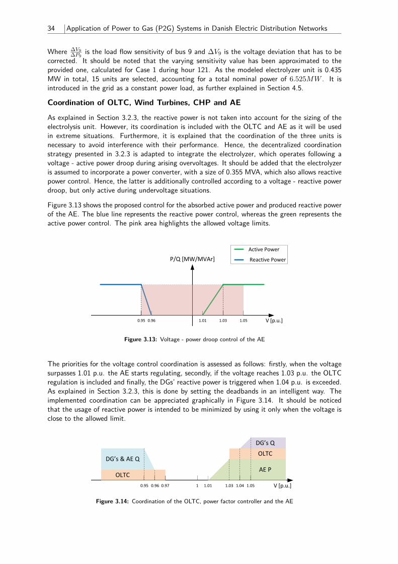
34 Application of Power to Gas (P2G) Systems in Danish Electric Distribution Networks
Where ∆V9∆P9
is the load flow sensitivity of bus 9 and ∆V9 is the voltage deviation that has to becorrected. It should be noted that the varying sensitivity value has been approximated to theprovided one, calculated for Case 1 during hour 121. As the modeled electrolyzer unit is 0.435MW in total, 15 units are selected, accounting for a total nominal power of 6.525MW . It isintroduced in the grid as a constant power load, as further explained in Section 4.5.
Coordination of OLTC, Wind Turbines, CHP and AE
As explained in Section 3.2.3, the reactive power is not taken into account for the sizing of theelectrolysis unit. However, its coordination is included with the OLTC and AE as it will be usedin extreme situations. Furthermore, it is explained that the coordination of the three units isnecessary to avoid interference with their performance. Hence, the decentralized coordinationstrategy presented in 3.2.3 is adapted to integrate the electrolyzer, which operates following avoltage - active power droop during arising overvoltages. It should be added that the electrolyzeris assumed to incorporate a power converter, with a size of 0.355 MVA, which also allows reactivepower control. Hence, the latter is additionally controlled according to a voltage - reactive powerdroop, but only active during undervoltage situations.
Figure 3.13 shows the proposed control for the absorbed active power and produced reactive powerof the AE. The blue line represents the reactive power control, whereas the green represents theactive power control. The pink area highlights the allowed voltage limits.
1.01 V [p.u.]1.030.95 0.96
P/Q [MW/MVAr]
Active Power
Reactive Power
V [p.u.]1.01 1.03 1.04 1.050.95 0.96 0.97
OLTC
OLTC
DG’s Q
AE P
DG’s & AE Q
1.05
1
Figure 3.13: Voltage - power droop control of the AE
The priorities for the voltage control coordination is assessed as follows: firstly, when the voltagesurpasses 1.01 p.u. the AE starts regulating, secondly, if the voltage reaches 1.03 p.u. the OLTCregulation is included and finally, the DGs’ reactive power is triggered when 1.04 p.u. is exceeded.As explained in Section 3.2.3, this is done by setting the deadbands in an intelligent way. Theimplemented coordination can be appreciated graphically in Figure 3.14. It should be noticedthat the usage of reactive power is intended to be minimized by using it only when the voltage isclose to the allowed limit.
1.01 V [p.u.]1.030.95 0.96
P/Q [MW/MVAr]
Active Power
Reactive Power
V [p.u.]1.01 1.03 1.04 1.050.95 0.96 0.97
OLTC
OLTC
DG’s Q
AE P
DG’s & AE Q
1.05
1
Figure 3.14: Coordination of the OLTC, power factor controller and the AE
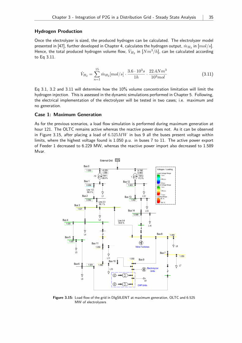
Chapter 3 - Integration of P2G in a Distribution Grid - Steady State Analysis 35
Hydrogen Production
Once the electrolyzer is sized, the produced hydrogen can be calculated. The electrolyzer modelpresented in [47], further developed in Chapter 4, calculates the hydrogen output, mH2 in [mol/s].Hence, the total produced hydrogen volume flow, VH2 in [Nm3/h], can be calculated accordingto Eq 3.11.
VH2 =15∑n=1
mH2 [mol/s] · 3.6 · 103s
1h · 22.4Nm3
103mol(3.11)
Eq 3.1, 3.2 and 3.11 will determine how the 10% volume concentration limitation will limit thehydrogen injection. This is assessed in the dynamic simulations performed in Chapter 5. Following,the electrical implementation of the electrolyzer will be tested in two cases; i.e. maximum andno generation.
Case 1: Maximum Generation
As for the previous scenarios, a load flow simulation is performed during maximum generation athour 121. The OLTC remains active whereas the reactive power does not. As it can be observedin Figure 3.15, after placing a load of 6.525MW in bus 9 all the buses present voltage withinlimits, where the highest voltage found is 1.050 p.u. in buses 7 to 11. The active power exportof Feeder 1 decreased to 6.229 MW, whereas the reactive power import also decreased to 1.589Mvar.
Voltages / Loading
Lower Voltage Range1. p.u....0.95 p.u....0.9 p.u.
Upper Voltage Range1. p.u....1.05 p.u....1.1 p.u.
Loading Range80. %...100. %
ElectrolyzerUnits
Wind Turbines
CHP UnitsT
erm
ina
l(7
)
Te
rmin
al(
6)
Terminal(5)
Terminal(4)
Terminal(3)
Terminal(2)
Terminal(1)
Terminal
Bus 91.050
Bus 14
0.999
Bus 131.002
Bus 6 1.020
Bus 71.050
Bus 8 1.050
Bus 101.050
Bus 111.050
Bus 5
1.020
Bus 2
0.992
Bus 41.020
Bus 31.021
Bus 121.003
Bus 1
0.958
Bus 0
1.000
Sta
tic
Ge
..6
5.3
%
SG~
Syn
chro
no
..2
9.6
%
SG~
Syn
chro
no
..2
9.6
%
2-Winding..70.5 %
2-Winding..70.5 %
Line 9-100.8 %
Lin
ec-
80
.0%
Static Ge..60.0 %
L9
L4
Bre
ake
r/S
..0
.0%
Lin
e1
4-c
0.0
%
Bre
ake
r/S
..0
.0%
Line 6-b0.0 %
Lin
eb-7
0.0
%
Lin
ea
-11
0.0
%
Lin
e4-a
0.0
%
Bre
ake
r/S
witch
0.0
%
Line 3-859.8 %
L8
Line 8-95.3 %
L10
L14
Lin
e1
3-1
44
.0%
L13
Line 12-134.1 %
L12
Lin
e5-6
0.4
%
L6
L7
Lin
e7-8
0.8
%
Lin
e1
0-1
10
.2%
L11
L5
Lin
e4
-51
.3%
Line 1-258.0 %
L1
Line 2-358.1 %
Lin
e3
-41
.5%
L3
TRF217.2 %
4.1980.983
1TRF126.8 %
-6.2291.589
-10
External Grid
DIgSILENT
Figure 3.15: Load flow of the grid in DIgSILENT at maximum generation, OLTC and 6.525MW of electrolyzers
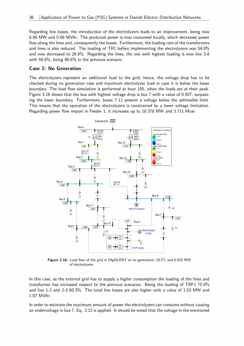
36 Application of Power to Gas (P2G) Systems in Danish Electric Distribution Networks
Regarding line losses, the introduction of the electrolyzers leads to an improvement, being now0.98 MW and 0.66 MVAr. The produced power is now consumed locally, which decreases powerflow along the lines and, consequently the losses. Furthermore, the loading rate of the transformersand lines is also reduced. The loading of TR1 before implementing the electrolyzers was 54.9%and now decreased to 26.8%. Regarding the lines, the one with highest loading is now line 3-8with 59.8%, being 96.6% in the previous scenario.
Case 2: No Generation
The electrolyzers represent an additional load to the grid; hence, the voltage drop has to bechecked during no generation case and maximum electrolyzer load in case it is below the lowerboundary. The load flow simulation is performed at hour 105, when the loads are at their peak.Figure 3.16 shows that the bus with highest voltage drop is bus 7 with a value of 0.927, surpass-ing the lower boundary. Furthermore, buses 7-11 present a voltage below the admissible limit.This means that the operation of the electrolyzers is constrained by a lower voltage limitation.Regarding power flow import in Feeder 1, it increases up to 18.378 MW and 3.711 Mvar.
Voltages / Loading
Lower Voltage Range1. p.u....0.95 p.u....0.9 p.u.
Upper Voltage Range1. p.u....1.05 p.u....1.1 p.u.
Loading Range80. %...100. %
ElectrolyzerUnits
Wind Turbines
CHP Units
Te
rmin
al(
7)
Te
rmin
al(
6)
Terminal(5)
Terminal(4)
Terminal(3)
Terminal(2)
Terminal(1)
Terminal
Bus 90.927
Bus 14
0.995
Bus 131.000
Bus 6 0.960
Bus 70.927
Bus 8 0.929
Bus 100.927
Bus 110.927
Bus 5
0.961
Bus 2
0.994
Bus 40.961
Bus 30.961
Bus 121.001
Bus 1
1.036
Bus 0
1.000
Sta
tic
Ge
..6
5.3
%
SG~
Syn
chro
no
..0
.0%
SG~
Syn
chro
no
..0
.0%
2-Winding..0.0 %
2-Winding..0.0 %
Line 9-101.3 %
Lin
ec-
80
.0%
Static Ge..0.0 %
L9
L4
Bre
ake
r/S
..0
.0%
Lin
e1
4-c
0.0
%
Bre
ake
r/S
..0
.0%
Line 6-b0.0 %
Lin
eb
-70
.0%
Lin
ea
-11
0.0
%
Lin
e4
-a0
.0%
Bre
ake
r/S
wit
ch0
.0%
Line 3-857.1 %
L8
Line 8-951.0 %
L10
L14
Lin
e1
3-1
47
.0%
L13
Line 12-138.3 %
L12
Lin
e5
-60
.6%
L6
L7
Lin
e7
-86
.3%
Lin
e1
0-1
10
.3%
L11
L5
Lin
e4
-51
.8%
Line 1-260.3 %
L1
Line 2-360.3 %
Lin
e3
-42
.0%
L3
TRF236.8 %
8.8332.543
1TRF175.0 %
18.3783.711
10
External Grid
DIgSILENT
Figure 3.16: Load flow of the grid in DIgSILENT at no generation, OLTC and 6.525 MWof electrolyzers
In this case, as the external grid has to supply a higher consumption the loading of the lines andtransformer has increased respect to the previous scenarios. Being the loading of TRF1 75.0%and line 1-2 and 2-3 60.3%. The total line losses are also higher with a value of 1.03 MW and1.07 MVAr.
In order to estimate the maximum amount of power the electrolyzers can consume without causingan undervoltage in bus 7, Eq. 3.12 is applied. It should be noted that the voltage in the mentioned
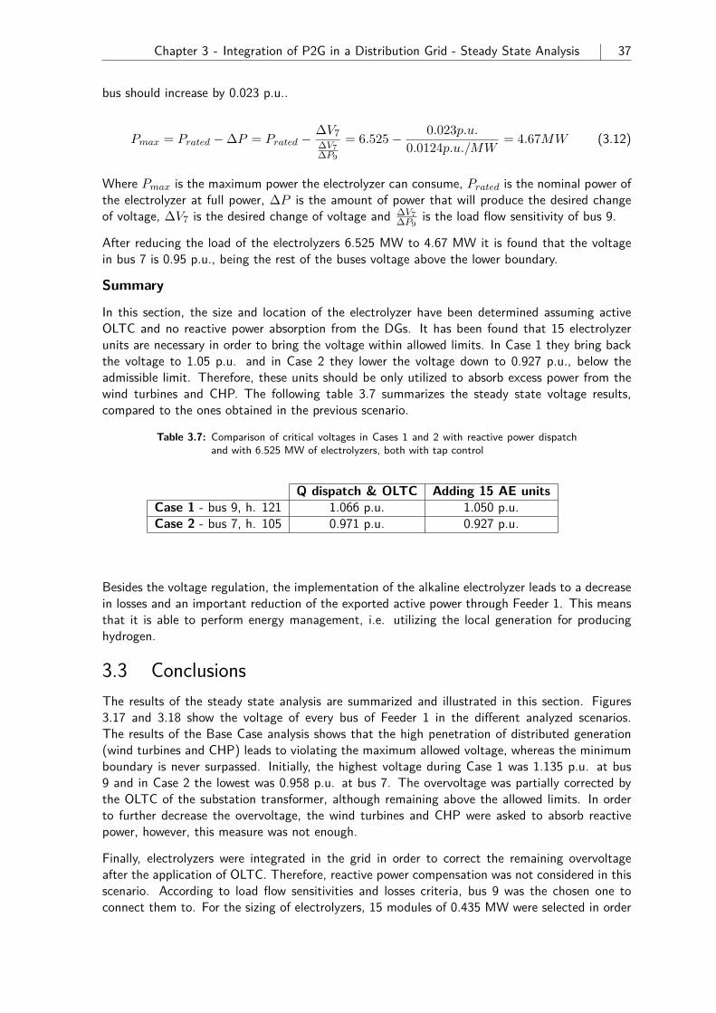
Chapter 3 - Integration of P2G in a Distribution Grid - Steady State Analysis 37
bus should increase by 0.023 p.u..
Pmax = Prated −∆P = Prated −∆V7∆V7∆P9
= 6.525− 0.023p.u.0.0124p.u./MW
= 4.67MW (3.12)
Where Pmax is the maximum power the electrolyzer can consume, Prated is the nominal power ofthe electrolyzer at full power, ∆P is the amount of power that will produce the desired changeof voltage, ∆V7 is the desired change of voltage and ∆V7
∆P9is the load flow sensitivity of bus 9.
After reducing the load of the electrolyzers 6.525 MW to 4.67 MW it is found that the voltagein bus 7 is 0.95 p.u., being the rest of the buses voltage above the lower boundary.
Summary
In this section, the size and location of the electrolyzer have been determined assuming activeOLTC and no reactive power absorption from the DGs. It has been found that 15 electrolyzerunits are necessary in order to bring the voltage within allowed limits. In Case 1 they bring backthe voltage to 1.05 p.u. and in Case 2 they lower the voltage down to 0.927 p.u., below theadmissible limit. Therefore, these units should be only utilized to absorb excess power from thewind turbines and CHP. The following table 3.7 summarizes the steady state voltage results,compared to the ones obtained in the previous scenario.
Table 3.7: Comparison of critical voltages in Cases 1 and 2 with reactive power dispatchand with 6.525 MW of electrolyzers, both with tap control
Q dispatch & OLTC Adding 15 AE unitsCase 1 - bus 9, h. 121 1.066 p.u. 1.050 p.u.Case 2 - bus 7, h. 105 0.971 p.u. 0.927 p.u.
Besides the voltage regulation, the implementation of the alkaline electrolyzer leads to a decreasein losses and an important reduction of the exported active power through Feeder 1. This meansthat it is able to perform energy management, i.e. utilizing the local generation for producinghydrogen.
3.3 ConclusionsThe results of the steady state analysis are summarized and illustrated in this section. Figures3.17 and 3.18 show the voltage of every bus of Feeder 1 in the different analyzed scenarios.The results of the Base Case analysis shows that the high penetration of distributed generation(wind turbines and CHP) leads to violating the maximum allowed voltage, whereas the minimumboundary is never surpassed. Initially, the highest voltage during Case 1 was 1.135 p.u. at bus9 and in Case 2 the lowest was 0.958 p.u. at bus 7. The overvoltage was partially corrected bythe OLTC of the substation transformer, although remaining above the allowed limits. In orderto further decrease the overvoltage, the wind turbines and CHP were asked to absorb reactivepower, however, this measure was not enough.
Finally, electrolyzers were integrated in the grid in order to correct the remaining overvoltageafter the application of OLTC. Therefore, reactive power compensation was not considered in thisscenario. According to load flow sensitivities and losses criteria, bus 9 was the chosen one toconnect them to. For the sizing of electrolyzers, 15 modules of 0.435 MW were selected in order
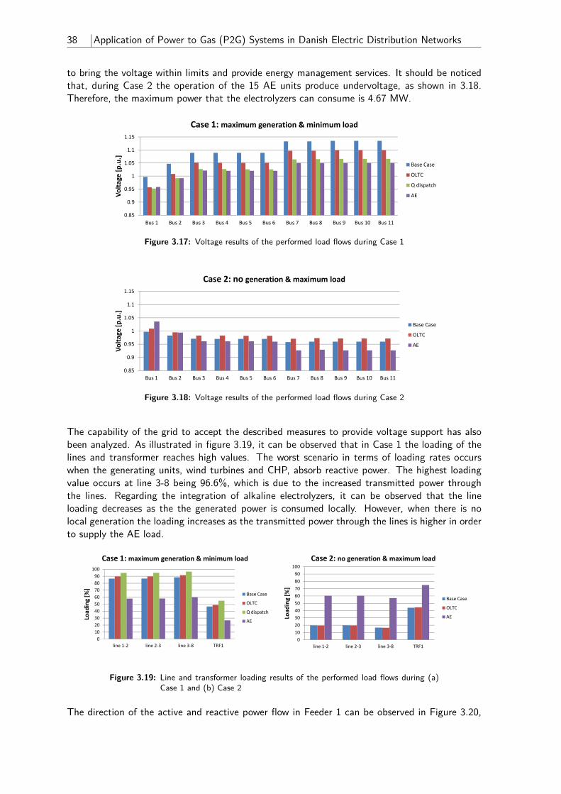
38 Application of Power to Gas (P2G) Systems in Danish Electric Distribution Networks
to bring the voltage within limits and provide energy management services. It should be noticedthat, during Case 2 the operation of the 15 AE units produce undervoltage, as shown in 3.18.Therefore, the maximum power that the electrolyzers can consume is 4.67 MW.
C 1 i ti & i i l d
1.1
1.15
Case 1: maximum generation & minimum load
1
1.05
age [p.u.]
Base Case
OLTC
Q di h
0 85
0.9
0.95
Volta Q dispatch
AE
0.85
Bus 1 Bus 2 Bus 3 Bus 4 Bus 5 Bus 6 Bus 7 Bus 8 Bus 9 Bus 10 Bus 11
Figure 3.17: Voltage results of the performed load flows during Case 1
1
1.05
1.1
1.15
ge [p
.u.]
Case 2: no generation & maximum load
Base Case
OLTC
0.85
0.9
0.95
Bus 1 Bus 2 Bus 3 Bus 4 Bus 5 Bus 6 Bus 7 Bus 8 Bus 9 Bus 10 Bus 11
Volta
OLTC
AE
Figure 3.18: Voltage results of the performed load flows during Case 2
The capability of the grid to accept the described measures to provide voltage support has alsobeen analyzed. As illustrated in figure 3.19, it can be observed that in Case 1 the loading of thelines and transformer reaches high values. The worst scenario in terms of loading rates occurswhen the generating units, wind turbines and CHP, absorb reactive power. The highest loadingvalue occurs at line 3-8 being 96.6%, which is due to the increased transmitted power throughthe lines. Regarding the integration of alkaline electrolyzers, it can be observed that the lineloading decreases as the the generated power is consumed locally. However, when there is nolocal generation the loading increases as the transmitted power through the lines is higher in orderto supply the AE load.
50
60
70
80
90
100
ing [%
]
Case 1: maximum generation & minimum load
Base Case
OLTC
0
10
20
30
40
line 1‐2 line 2‐3 line 3‐8 TRF1
Load
i
Q dispatch
AE
50
60
70
80
90
100
ing [%
]
Case 2: no generation & maximum load
Base Case
OL C
0
10
20
30
40
line 1‐2 line 2‐3 line 3‐8 TRF1
Load OLTC
AE
Figure 3.19: Line and transformer loading results of the performed load flows during (a)Case 1 and (b) Case 2
The direction of the active and reactive power flow in Feeder 1 can be observed in Figure 3.20,
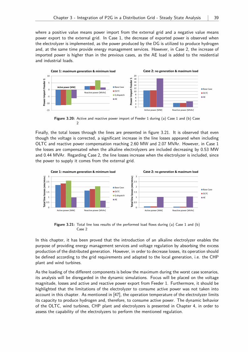
Chapter 3 - Integration of P2G in a Distribution Grid - Steady State Analysis 39
where a positive value means power import from the external grid and a negative value meanspower export to the external grid. In Case 1, the decrease of exported power is observed whenthe electrolyzer is implemented, as the power produced by the DG is utilized to produce hydrogenand, at the same time provide energy management services. However, in Case 2, the increase ofimported power is higher than in the previous cases, as the AE load is added to the residentialand industrial loads.
0
5
10
Active power [MW]
Reactive power [MVAr]ort Feede
r 1
Case 1: maximum generation & minimum load
Base Case
OLTC
‐15
‐10
‐5
Active power [MW]
Reactive power [MVAr]
Power Im
po Q dispatch
AE
10
12
14
16
18
20
ort Feede
r 1
Case 2: no generation & maximum load
Base Case
OL C
0
2
4
6
8
Active power [MW] Reactive power [MVAr]
Power Im
p OLTC
AE
Figure 3.20: Active and reactive power import of Feeder 1 during (a) Case 1 and (b) Case2
Finally, the total losses through the lines are presented in figure 3.21. It is observed that eventhough the voltage is corrected, a significant increase in the line losses appeared when includingOLTC and reactive power compensation reaching 2.60 MW and 2.07 MVAr. However, in Case 1the losses are compensated when the alkaline electrolyzers are included decreasing by 0.53 MWand 0.44 MVAr. Regarding Case 2, the line losses increase when the electrolyzer is included, sincethe power to supply it comes from the external grid.
1.5
2
2.5
3
sses [M
W/M
VAr]
Case 1: maximum generation & minimum load
Base Case
OLTC
0
0.5
1
Active power [MW] Reactive power [MVAr]
Total line los
Q dispatch
AE
1.5
2
2.5
3
sses [M
W/M
VAr]
Case 2: no generation & maximum load
Base Case
OL C
0
0.5
1
Active power [MW] Reactive power [MVAr]
Total line los OLTC
AE
Figure 3.21: Total line loss results of the performed load flows during (a) Case 1 and (b)Case 2
In this chapter, it has been proved that the introduction of an alkaline electrolyzer enables thepurpose of providing energy management services and voltage regulation by absorbing the excessproduction of the distributed generation. However, in order to decrease losses, its operation shouldbe defined according to the grid requirements and adapted to the local generation, i.e. the CHPplant and wind turbines.
As the loading of the different components is below the maximum during the worst case scenarios,its analysis will be disregarded in the dynamic simulations. Focus will be placed on the voltagemagnitude, losses and active and reactive power export from Feeder 1. Furthermore, it should behighlighted that the limitations of the electrolyzer to consume active power was not taken intoaccount in this chapter. As mentioned in [47], the operation temperature of the electrolyzer limitsits capacity to produce hydrogen and, therefore, to consume active power. The dynamic behaviorof the OLTC, wind turbines, CHP plant and electrolyzers is presented in Chapter 4, in order toassess the capability of the electrolyzers to perform the mentioned regulation.

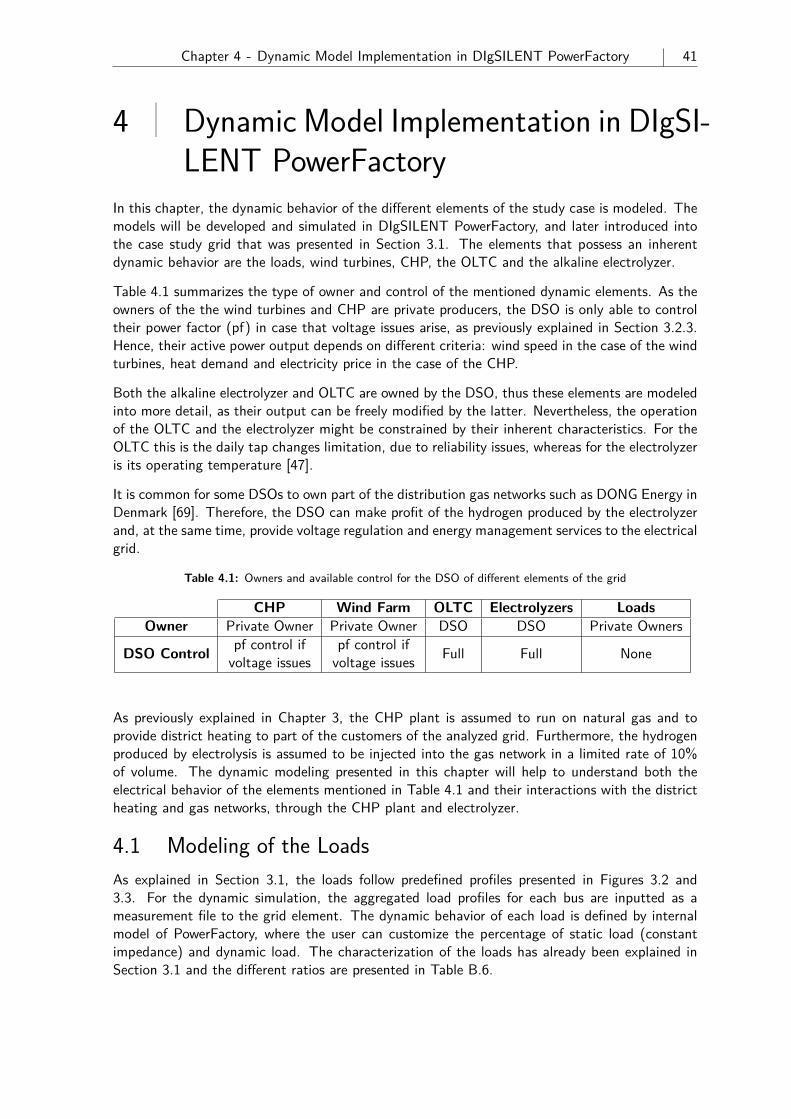
Chapter 4 - Dynamic Model Implementation in DIgSILENT PowerFactory 41
4 Dynamic Model Implementation in DIgSI-LENT PowerFactory
In this chapter, the dynamic behavior of the different elements of the study case is modeled. Themodels will be developed and simulated in DIgSILENT PowerFactory, and later introduced intothe case study grid that was presented in Section 3.1. The elements that possess an inherentdynamic behavior are the loads, wind turbines, CHP, the OLTC and the alkaline electrolyzer.
Table 4.1 summarizes the type of owner and control of the mentioned dynamic elements. As theowners of the the wind turbines and CHP are private producers, the DSO is only able to controltheir power factor (pf) in case that voltage issues arise, as previously explained in Section 3.2.3.Hence, their active power output depends on different criteria: wind speed in the case of the windturbines, heat demand and electricity price in the case of the CHP.
Both the alkaline electrolyzer and OLTC are owned by the DSO, thus these elements are modeledinto more detail, as their output can be freely modified by the latter. Nevertheless, the operationof the OLTC and the electrolyzer might be constrained by their inherent characteristics. For theOLTC this is the daily tap changes limitation, due to reliability issues, whereas for the electrolyzeris its operating temperature [47].
It is common for some DSOs to own part of the distribution gas networks such as DONG Energy inDenmark [69]. Therefore, the DSO can make profit of the hydrogen produced by the electrolyzerand, at the same time, provide voltage regulation and energy management services to the electricalgrid.
Table 4.1: Owners and available control for the DSO of different elements of the grid
CHP Wind Farm OLTC Electrolyzers LoadsOwner Private Owner Private Owner DSO DSO Private Owners
DSO Control pf control ifvoltage issues
pf control ifvoltage issues Full Full None
As previously explained in Chapter 3, the CHP plant is assumed to run on natural gas and toprovide district heating to part of the customers of the analyzed grid. Furthermore, the hydrogenproduced by electrolysis is assumed to be injected into the gas network in a limited rate of 10%of volume. The dynamic modeling presented in this chapter will help to understand both theelectrical behavior of the elements mentioned in Table 4.1 and their interactions with the districtheating and gas networks, through the CHP plant and electrolyzer.
4.1 Modeling of the LoadsAs explained in Section 3.1, the loads follow predefined profiles presented in Figures 3.2 and3.3. For the dynamic simulation, the aggregated load profiles for each bus are inputted as ameasurement file to the grid element. The dynamic behavior of each load is defined by internalmodel of PowerFactory, where the user can customize the percentage of static load (constantimpedance) and dynamic load. The characterization of the loads has already been explained inSection 3.1 and the different ratios are presented in Table B.6.
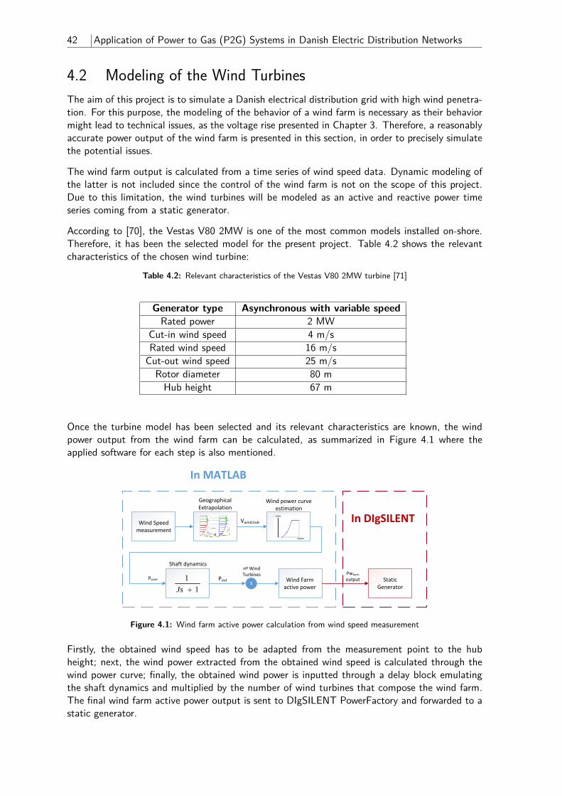
42 Application of Power to Gas (P2G) Systems in Danish Electric Distribution Networks
4.2 Modeling of the Wind TurbinesThe aim of this project is to simulate a Danish electrical distribution grid with high wind penetra-tion. For this purpose, the modeling of the behavior of a wind farm is necessary as their behaviormight lead to technical issues, as the voltage rise presented in Chapter 3. Therefore, a reasonablyaccurate power output of the wind farm is presented in this section, in order to precisely simulatethe potential issues.
The wind farm output is calculated from a time series of wind speed data. Dynamic modeling ofthe latter is not included since the control of the wind farm is not on the scope of this project.Due to this limitation, the wind turbines will be modeled as an active and reactive power timeseries coming from a static generator.
According to [70], the Vestas V80 2MW is one of the most common models installed on-shore.Therefore, it has been the selected model for the present project. Table 4.2 shows the relevantcharacteristics of the chosen wind turbine:
Table 4.2: Relevant characteristics of the Vestas V80 2MW turbine [71]
Generator type Asynchronous with variable speedRated power 2 MW
Cut-in wind speed 4 m/sRated wind speed 16 m/sCut-out wind speed 25 m/sRotor diameter 80 mHub height 67 m
Once the turbine model has been selected and its relevant characteristics are known, the windpower output from the wind farm can be calculated, as summarized in Figure 4.1 where theapplied software for each step is also mentioned.
Geographical Extrapolation
Wind Speed measurement
Wind power curve estimation
Vwind,hub
Pwind
11Js
Shaft dynamicsnº Wind Turbines
PoutX
Wind Farm active power
Static Generator
Pwfarm output
In MATLAB
In DIgSILENT
Figure 4.1: Wind farm active power calculation from wind speed measurement
Firstly, the obtained wind speed has to be adapted from the measurement point to the hubheight; next, the wind power extracted from the obtained wind speed is calculated through thewind power curve; finally, the obtained wind power is inputted through a delay block emulatingthe shaft dynamics and multiplied by the number of wind turbines that compose the wind farm.The final wind farm active power output is sent to DIgSILENT PowerFactory and forwarded to astatic generator.
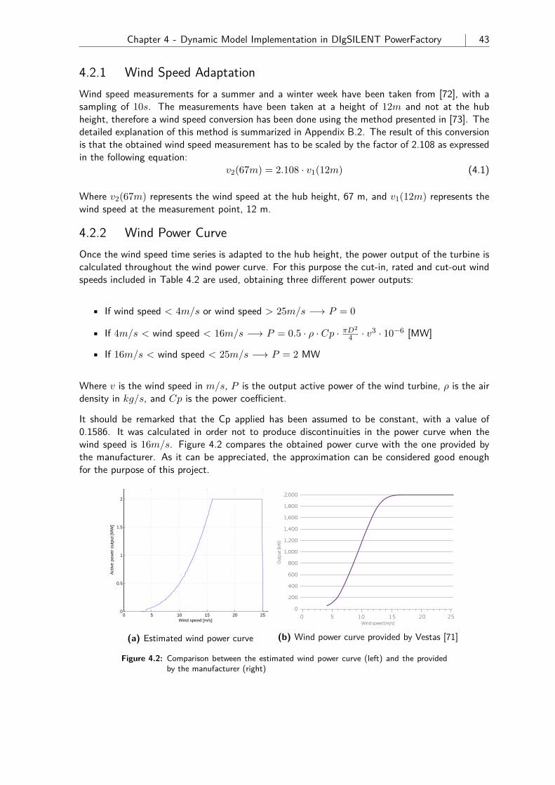
Chapter 4 - Dynamic Model Implementation in DIgSILENT PowerFactory 43
4.2.1 Wind Speed AdaptationWind speed measurements for a summer and a winter week have been taken from [72], with asampling of 10s. The measurements have been taken at a height of 12m and not at the hubheight, therefore a wind speed conversion has been done using the method presented in [73]. Thedetailed explanation of this method is summarized in Appendix B.2. The result of this conversionis that the obtained wind speed measurement has to be scaled by the factor of 2.108 as expressedin the following equation:
v2(67m) = 2.108 · v1(12m) (4.1)
Where v2(67m) represents the wind speed at the hub height, 67 m, and v1(12m) represents thewind speed at the measurement point, 12 m.
4.2.2 Wind Power CurveOnce the wind speed time series is adapted to the hub height, the power output of the turbine iscalculated throughout the wind power curve. For this purpose the cut-in, rated and cut-out windspeeds included in Table 4.2 are used, obtaining three different power outputs:
• If wind speed < 4m/s or wind speed > 25m/s −→ P = 0
• If 4m/s < wind speed < 16m/s −→ P = 0.5 · ρ · Cp · πD2
4 · v3 · 10−6 [MW]
• If 16m/s < wind speed < 25m/s −→ P = 2 MW
Where v is the wind speed in m/s, P is the output active power of the wind turbine, ρ is the airdensity in kg/s, and Cp is the power coefficient.
It should be remarked that the Cp applied has been assumed to be constant, with a value of0.1586. It was calculated in order not to produce discontinuities in the power curve when thewind speed is 16m/s. Figure 4.2 compares the obtained power curve with the one provided bythe manufacturer. As it can be appreciated, the approximation can be considered good enoughfor the purpose of this project.
0 5 10 15 20 250
0.5
1
1.5
2
Wind speed [m/s]
Act
ive
pow
er o
utpu
t [M
W]
(a) Estimated wind power curve
teChniCAl dAtA for V80-2.0 MW
Copyright NoticeThis document is created by Vestas Wind Systems A/S and contains copyrightedmaterial, trademarks, and other proprietary information. All rights reserved. Nopart of the documents may be reproduced or copied in any form or by any meanssuch as graphic, electronic, or mechanical, including photocopying, taping, orinformation storage and retrieval systems without the prior written permission ofVestas Wind Systems A/S.
All specifications are for informational purposes and are subject to changewithout notice. Vestas does not make any representations or extend anywarranties, expressed or implied, as to the adequacy or accuracy of thisinformation.VCS turbines are not available in the USA or Canada.
Power regulation pitch regulated with variable speed
Operating dataRated power 2,000 kWCut-in wind speed 4 m/sRated wind speed 16 m/sCut-out wind speed 25 m/sWind Class IEC IAOperating temperature standard range -20°C to 40°C low temperature option -30°C to 40°C
RotorRotor diameter 80 mSwept area 5,027 m2
Nominal revolutions 16.7 rpmOperational interval 10.8-19.1 rpmAir brake full blade feathering with 3 pitch cylinders
TowerType tubular steel towerHub heights 60 m, 67 m, 78 m, 80 m and 100 m
GeneratorType 4-pole asynchronous with variable speedNominal output 2,000 kWOperational data 50 Hz/60 Hz 690 V
GearboxType 3-stage planetary/helical
Power curve V80-2.0 MWNoise reduced sound power modes are available.
Main dimensions
BladeLength 39 mMax. chord 3.5 mBlade 6,500 kg
NacelleHeight for transport 4 mHeight installed(including CoolerTop™) 5.4 mLength 10.4 mWidth 3.4 mWeight 69 metric tonnes
HubMax. diameter 3.3 mMax. width 4 mLength 4.2 mWeight 18 metric tonnes
Tower
60 m (IEC IA)Weight 137 metric tonnes
67 m (IEC IIA)Weight 116 metric tonnes
78 m (IEC IA)Weight 153 metric tonnes
80 m (IEC IIA)Weight 148 metric tonnes
100 m (DiBt II)Weight 198 metric tonnes
Ou
tpu
t (k
W)
2,000
1,800
1,600
1,400
1,200
1,000
800
600
400
200
0
Wind speed (m/s)
0 5 10 15 20 25
(b) Wind power curve provided by Vestas [71]
Figure 4.2: Comparison between the estimated wind power curve (left) and the providedby the manufacturer (right)
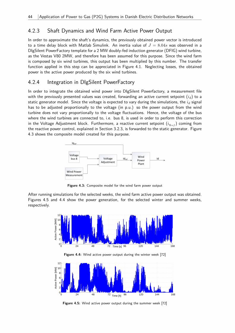
44 Application of Power to Gas (P2G) Systems in Danish Electric Distribution Networks
4.2.3 Shaft Dynamics and Wind Farm Active Power OutputIn order to approximate the shaft’s dynamics, the previously obtained power vector is introducedto a time delay block with Matlab Simulink. An inertia value of J = 8.04s was observed in aDIgSilent PowerFactory template for a 2 MW doubly-fed induction generator (DFIG) wind turbine,as the Vestas V80 2MW, and therefore has been assumed for this purpose. Since the wind farmis composed by six wind turbines, this output has been multiplied by this number. The transferfunction applied in this step can be appreciated in Figure 4.1. Neglecting losses, the obtainedpower is the active power produced by the six wind turbines.
4.2.4 Integration in DIgSilent PowerFactoryIn order to integrate the obtained wind power into DIgSilent Powerfactory, a measurement filewith the previously presented values was created, forwarding an active current setpoint (id) to astatic generator model. Since the voltage is expected to vary during the simulations, the id signalhas to be adjusted proportionally to the voltage (in p.u.) so the power output from the windturbine does not vary proportionally to the voltage fluctuations. Hence, the voltage of the buswhere the wind turbines are connected to, i.e. bus 8, is used in order to perform this correctionin the Voltage Adjustment block. Furthermore, a reactive current setpoint (iqref
) coming fromthe reactive power control, explained in Section 3.2.3, is forwarded to the static generator. Figure4.3 shows the composite model created for this purpose.
Wind Power Plant
Idref
Voltage bus 8 Voltage
Adjustment
Wind Power Measurement
Iqref
Id
Figure 4.3: Composite model for the wind farm power output
After running simulations for the selected weeks, the wind farm active power output was obtained.Figures 4.5 and 4.4 show the power generation, for the selected winter and summer weeks,respectively.
0 24 48 72 96 120 144 1680
2
4
6
8
10
12
Time [s]
Act
ive
Pow
er [M
W]
Figure 4.4: Wind active power output during the winter week [72]
0 24 48 72 96 120 144 1680
2
4
6
8
10
12
Time [h]
Act
ive
Pow
er [M
W]
Figure 4.5: Wind active power output during the summer week [72]
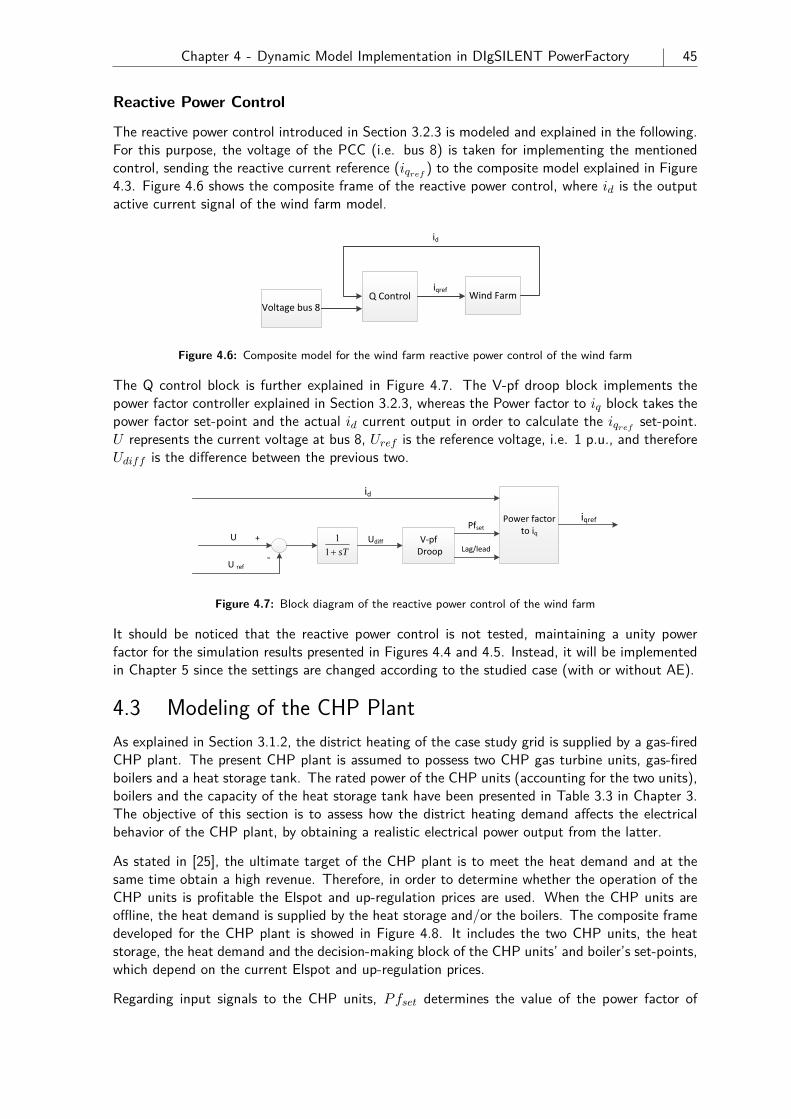
Chapter 4 - Dynamic Model Implementation in DIgSILENT PowerFactory 45
Reactive Power Control
The reactive power control introduced in Section 3.2.3 is modeled and explained in the following.For this purpose, the voltage of the PCC (i.e. bus 8) is taken for implementing the mentionedcontrol, sending the reactive current reference (iqref
) to the composite model explained in Figure4.3. Figure 4.6 shows the composite frame of the reactive power control, where id is the outputactive current signal of the wind farm model.
iqrefQ Control Wind Farm
Voltage bus 8
id
Figure 4.6: Composite model for the wind farm reactive power control of the wind farm
The Q control block is further explained in Figure 4.7. The V-pf droop block implements thepower factor controller explained in Section 3.2.3, whereas the Power factor to iq block takes thepower factor set-point and the actual id current output in order to calculate the iqref
set-point.U represents the current voltage at bus 8, Uref is the reference voltage, i.e. 1 p.u., and thereforeUdiff is the difference between the previous two.
U ref‐
+UPfset
Lag/lead1
1 sTV‐pf
Droop
id
Udiff
Power factor to iq
iqref
Figure 4.7: Block diagram of the reactive power control of the wind farm
It should be noticed that the reactive power control is not tested, maintaining a unity powerfactor for the simulation results presented in Figures 4.4 and 4.5. Instead, it will be implementedin Chapter 5 since the settings are changed according to the studied case (with or without AE).
4.3 Modeling of the CHP PlantAs explained in Section 3.1.2, the district heating of the case study grid is supplied by a gas-firedCHP plant. The present CHP plant is assumed to possess two CHP gas turbine units, gas-firedboilers and a heat storage tank. The rated power of the CHP units (accounting for the two units),boilers and the capacity of the heat storage tank have been presented in Table 3.3 in Chapter 3.The objective of this section is to assess how the district heating demand affects the electricalbehavior of the CHP plant, by obtaining a realistic electrical power output from the latter.
As stated in [25], the ultimate target of the CHP plant is to meet the heat demand and at thesame time obtain a high revenue. Therefore, in order to determine whether the operation of theCHP units is profitable the Elspot and up-regulation prices are used. When the CHP units areoffline, the heat demand is supplied by the heat storage and/or the boilers. The composite framedeveloped for the CHP plant is showed in Figure 4.8. It includes the two CHP units, the heatstorage, the heat demand and the decision-making block of the CHP units’ and boiler’s set-points,which depend on the current Elspot and up-regulation prices.
Regarding input signals to the CHP units, Pfset determines the value of the power factor of
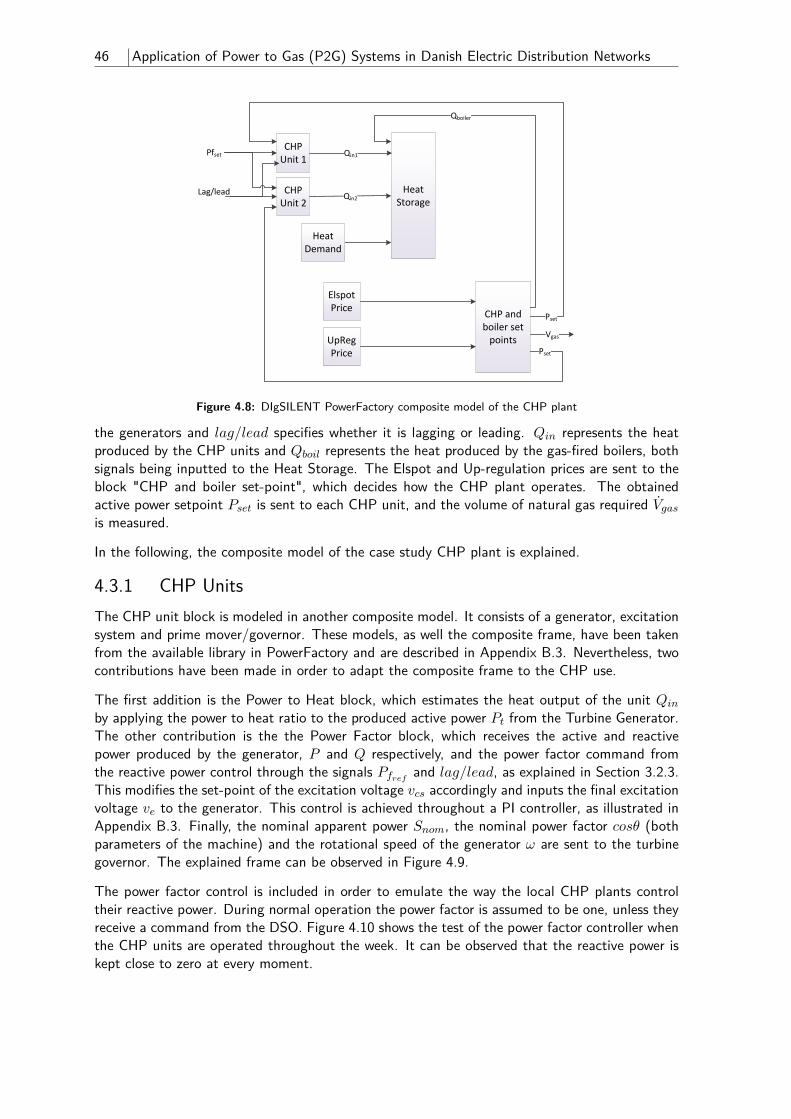
46 Application of Power to Gas (P2G) Systems in Danish Electric Distribution Networks
Elspot Price
UpReg Price
Heat Storage
Heat Demand
CHP Unit 2
Qin1CHP Unit 1
Pset
Pset
Qboiler
Qin2
CHP and boiler set points
Pfset
Lag/lead
Vgas
Figure 4.8: DIgSILENT PowerFactory composite model of the CHP plant
the generators and lag/lead specifies whether it is lagging or leading. Qin represents the heatproduced by the CHP units and Qboil represents the heat produced by the gas-fired boilers, bothsignals being inputted to the Heat Storage. The Elspot and Up-regulation prices are sent to theblock "CHP and boiler set-point", which decides how the CHP plant operates. The obtainedactive power setpoint Pset is sent to each CHP unit, and the volume of natural gas required Vgasis measured.
In the following, the composite model of the case study CHP plant is explained.
4.3.1 CHP UnitsThe CHP unit block is modeled in another composite model. It consists of a generator, excitationsystem and prime mover/governor. These models, as well the composite frame, have been takenfrom the available library in PowerFactory and are described in Appendix B.3. Nevertheless, twocontributions have been made in order to adapt the composite frame to the CHP use.
The first addition is the Power to Heat block, which estimates the heat output of the unit Qinby applying the power to heat ratio to the produced active power Pt from the Turbine Generator.The other contribution is the the Power Factor block, which receives the active and reactivepower produced by the generator, P and Q respectively, and the power factor command fromthe reactive power control through the signals Pfref
and lag/lead, as explained in Section 3.2.3.This modifies the set-point of the excitation voltage vcs accordingly and inputs the final excitationvoltage ve to the generator. This control is achieved throughout a PI controller, as illustrated inAppendix B.3. Finally, the nominal apparent power Snom, the nominal power factor cosθ (bothparameters of the machine) and the rotational speed of the generator ω are sent to the turbinegovernor. The explained frame can be observed in Figure 4.9.
The power factor control is included in order to emulate the way the local CHP plants controltheir reactive power. During normal operation the power factor is assumed to be one, unless theyreceive a command from the DSO. Figure 4.10 shows the test of the power factor controller whenthe CHP units are operated throughout the week. It can be observed that the reactive power iskept close to zero at every moment.
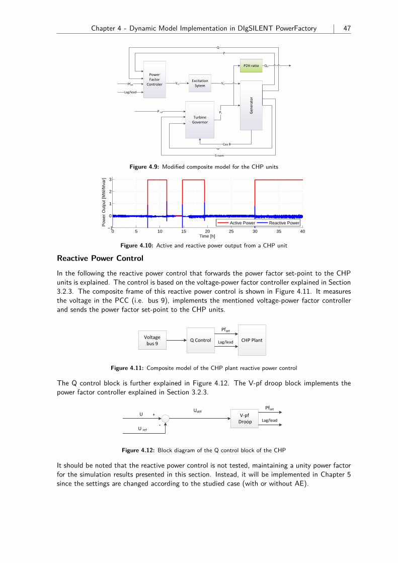
Chapter 4 - Dynamic Model Implementation in DIgSILENT PowerFactory 47
Ve
ω
Excitation Sytem
TurbineGovernor
Cos θ
S nom
P ref Pt
P2H ratio
Power Factor
Controler
P
Q
Qin
Gen
erator
VcsPfset
Lag/lead
Figure 4.9: Modified composite model for the CHP units
0 5 10 15 20 25 30 35 40−1
0
1
2
3
Time [h]
Pow
er O
utpu
t [M
W/M
var]
Active Power Reactive Power
Figure 4.10: Active and reactive power output from a CHP unit
Reactive Power Control
In the following the reactive power control that forwards the power factor set-point to the CHPunits is explained. The control is based on the voltage-power factor controller explained in Section3.2.3. The composite frame of this reactive power control is shown in Figure 4.11. It measuresthe voltage in the PCC (i.e. bus 9), implements the mentioned voltage-power factor controllerand sends the power factor set-point to the CHP units.
Pfset
Lag/leadQ Control CHP PlantVoltage
bus 9
Figure 4.11: Composite model of the CHP plant reactive power control
The Q control block is further explained in Figure 4.12. The V-pf droop block implements thepower factor controller explained in Section 3.2.3.
U ref‐
+UPfset
Lag/leadV‐pf
Droop
Udiff
Figure 4.12: Block diagram of the Q control block of the CHP
It should be noted that the reactive power control is not tested, maintaining a unity power factorfor the simulation results presented in this section. Instead, it will be implemented in Chapter 5since the settings are changed according to the studied case (with or without AE).
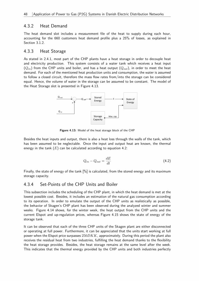
48 Application of Power to Gas (P2G) Systems in Danish Electric Distribution Networks
4.3.2 Heat DemandThe heat demand slot includes a measurement file of the heat to supply during each hour,accounting for the 660 customers heat demand profile plus a 25% of losses, as explained inSection 3.1.2.
4.3.3 Heat StorageAs stated in 2.4.1, most part of the CHP plants have a heat storage in order to decouple heatand electricity production. This system consists of a water tank which receives a heat input(Qin) from the CHP units and boiler, and has a heat output (Qout), in order to meet the heatdemand. For each of the mentioned heat production units and consumption, the water is assumedto follow a closed circuit, therefore the mass flow rates from/into the storage can be consideredequal. Hence, the volume of water in the storage can be assumed to be constant. The model ofthe Heat Storage slot is presented in Figure 4.13.
State of Energy
Q diff
Q in
‐
+
Q out
Storage Capacity
Stored Energy
E
Max. cap
Figure 4.13: Model of the heat storage block of the CHP
Besides the heat inputs and output, there is also a heat loss through the walls of the tank, whichhas been assumed to be neglectable. Once the input and output heat are known, the thermalenergy in the tank (E) can be calculated according to equation 4.2:
Qin −Qout = dE
dt(4.2)
Finally, the state of energy of the tank [%] is calculated, from the stored energy and its maximumstorage capacity.
4.3.4 Set-Points of the CHP Units and BoilerThis subsection includes the scheduling of the CHP plant, in which the heat demand is met at thelowest possible cost. Besides, it includes an estimation of the natural gas consumption accordingto its operation. In order to emulate the output of the CHP units as realistically as possible,the behavior of Skagen’s CHP plant has been observed during the analyzed winter and summerweeks. Figure 4.14 shows, for the winter week, the heat output from the CHP units and thecurrent Elspot and up-regulation prices, whereas Figure 4.15 shows the state of energy of thestorage tank.
It can be observed that each of the three CHP units of the Skagen plant are either disconnectedor operating at full power. Furthermore, it can be appreciated that the units start working at fullpower when the Elspot price surpasses 250DKK, approximately. During this period the plant alsoreceives the residual heat from two industries, fulfilling the heat demand thanks to the flexibilitythe heat storage provides. Besides, the heat storage remains at the same level after the week.This indicates that the thermal energy provided by the CHP units and both industries perfectly
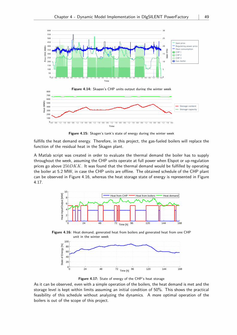
Chapter 4 - Dynamic Model Implementation in DIgSILENT PowerFactory 49
31/3/2015 Skagen Varmeværk
http://www.emd.dk/desire/skagen/ 1/1
This page is hosted and maintained by EMD International A/S
Time
Time
Pric
e (D
KK/M
Wh)
Heat (M
W)
Spot priceRegulating power price Heat consumptionCHP 1CHP 2CHP 3Gas-boiler
00 06 12 18 00 06 12 18 00 06 12 18 00 06 12 18 00 06 12 18 00 06 12 18 00 06 12 18 00
00 06 12 18 00 06 12 18 00 06 12 18 00 06 12 18 00 06 12 18 00 06 12 18 00 06 12 18 00
0
50
100
150
200
250
300
350
400
450
500
550
600
0
10
20
30
5
15
25
0
100
200
300
Figure 4.14: Skagen’s CHP units output during the winter week
31/3/2015 Skagen Varmeværk
http://www.emd.dk/desire/skagen/ 1/1
Current7 days CO2emission
International A/S
Time
Heat (M
W)
Hea
t (M
Wh)
Skagen District Heating, Monday, 2014-01-20 to Sunday, 2014-01-26
Spot priceRegulating power price Heat consumptionCHP 1CHP 2CHP 3
00 06 12 18 00 06 12 18 00 06 12 18 00 06 12 18 00 06 12 18 00 06 12 18 00 06 12 18 00
250
300
350
400
450
500
550
600
20
30
15
25
0
100
200
300
400
500
600
700
800
Storage contentStorage capacity
Figure 4.15: Skagen’s tank’s state of energy during the winter week
fulfills the heat demand energy. Therefore, in this project, the gas-fueled boilers will replace thefunction of the residual heat in the Skagen plant.
A Matlab script was created in order to evaluate the thermal demand the boiler has to supplythroughout the week, assuming the CHP units operate at full power when Elspot or up-regulationprices go above 250DKK. It was found that the thermal demand would be fulfilled by operatingthe boiler at 5.2 MW, in case the CHP units are offline. The obtained schedule of the CHP plantcan be observed in Figure 4.16, whereas the heat storage state of energy is represented in Figure4.17.
0 24 48 72 96 120 144 1680
2
4
6
8
10
Time [h]
Hea
t Inp
ut/O
utpu
t [M
W]
Heat from CHP Heat from boilers Heat demand
Figure 4.16: Heat demand, generated heat from boilers and generated heat from one CHPunit in the winter week
0 24 48 72 96 120 144 1680
20
40
60
80
100
Time [h]
Sta
te o
f Ene
rgy
[%]
Figure 4.17: State of energy of the CHP’s heat storageAs it can be observed, even with a simple operation of the boilers, the heat demand is met and thestorage level is kept within limits assuming an initial condition of 50%. This shows the practicalfeasibility of this schedule without analyzing the dynamics. A more optimal operation of theboilers is out of the scope of this project.
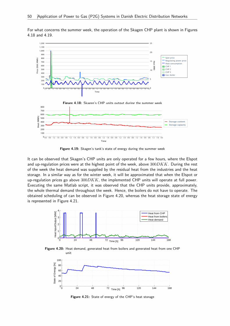
50 Application of Power to Gas (P2G) Systems in Danish Electric Distribution Networks
For what concerns the summer week, the operation of the Skagen CHP plant is shown in Figures4.18 and 4.19.
31/3/2015 Skagen Varmeværk
http://www.emd.dk/desire/skagen/ 1/1
This page is hosted and maintained by EMD International A/S
Time
Time
Pric
e (D
KK/M
Wh)
Heat (M
W)
H
00 06 12 18 00 06 12 18 00 06 12 18 00 06 12 18 00 06 12 18 00 06 12 18 00 06 12 18 00
00 06 12 18 00 06 12 18 00 06 12 18 00 06 12 18 00 06 12 18 00 06 12 18 00 06 12 18 00
0
100
200
300
400
500
600
700
800
900
1,000
1,100
1,200
0
5
10
15
20
25
0
100
200
300
Spot priceRegulating power price Heat consumptionCHP 1CHP 2CHP 3Gas-boiler
Figure 4.18: Skagen’s CHP units output during the summer week
31/3/2015 Skagen Varmeværk
http://www.emd.dk/desire/skagen/ 1/1
Current7 days CO2emission
EMD International A/S
Time
rice
(DKK
/MW
h)
Heat(M
W)
Hea
t (M
Wh)
Skagen District Heating, Monday, 2014-07-28 to Sunday, 2014-08-03
Spot priceRegulating power price, UpRegulating power price, DownPositive Primary ReserveNegative Primary Reserve
ption
aste IncinerationSkagen
00 06 12 18 00 06 12 18 00 06 12 18 00 06 12 18 00 06 12 18 00 06 12 18 00 06 12 18 00
500
600
700
800
900
1,000
1,100
1,200
10
15
20
25
0
100
200
300
400
500
600
700
800
Storage contentStorage capacity
Figure 4.19: Skagen’s tank’s state of energy during the summer week
It can be observed that Skagen’s CHP units are only operated for a few hours, where the Elspotand up-regulation prices were at the highest point of the week, above 300DKK. During the restof the week the heat demand was supplied by the residual heat from the industries and the heatstorage. In a similar way as for the winter week, it will be approximated that when the Elspot orup-regulation prices go above 300DKK, the implemented CHP units will operate at full power.Executing the same Matlab script, it was observed that the CHP units provide, approximately,the whole thermal demand throughout the week. Hence, the boilers do not have to operate. Theobtained scheduling of can be observed in Figure 4.20, whereas the heat storage state of energyis represented in Figure 4.21.
0 24 48 72 96 120 144 1680
1
2
3
4
Time [h]
Hea
t Inp
ut/O
utpu
t [M
W]
Heat from CHPHeat from boilersHeat demand
Figure 4.20: Heat demand, generated heat from boilers and generated heat from one CHPunit
0 24 48 72 96 120 144 1680
20
40
60
80
100
Time [h]
Sta
te o
f Ene
rgy
[%]
Figure 4.21: State of energy of the CHP’s heat storage
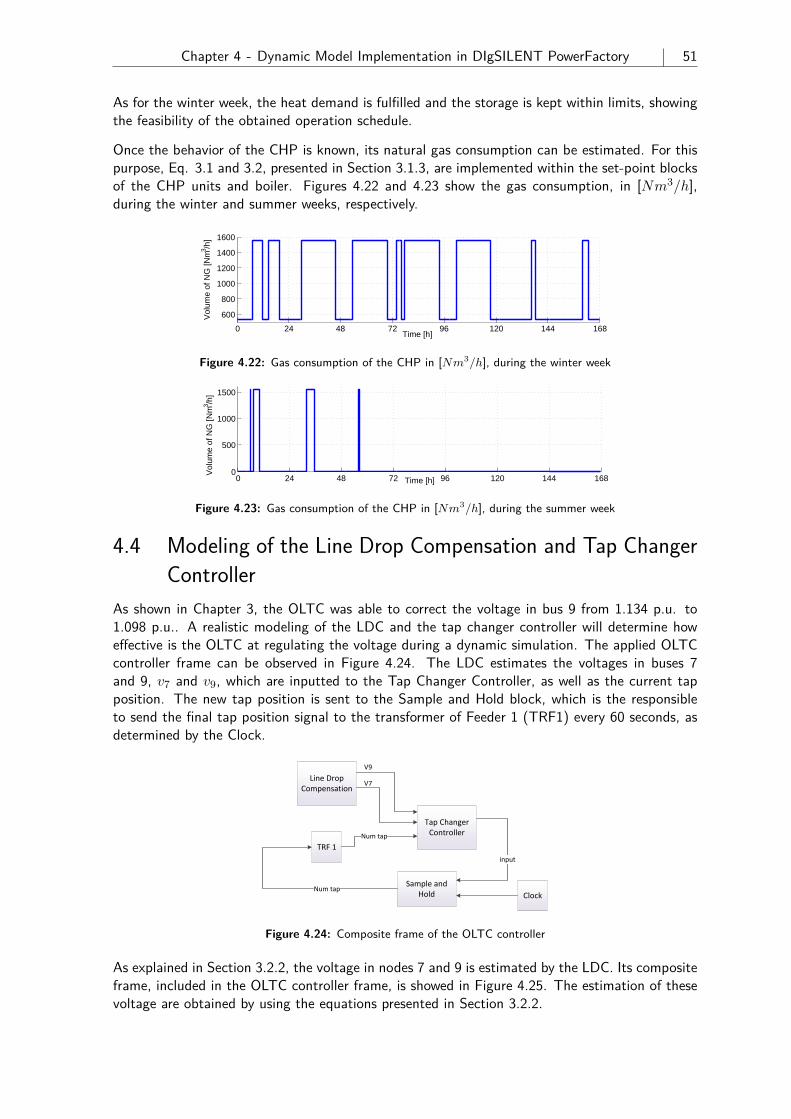
Chapter 4 - Dynamic Model Implementation in DIgSILENT PowerFactory 51
As for the winter week, the heat demand is fulfilled and the storage is kept within limits, showingthe feasibility of the obtained operation schedule.
Once the behavior of the CHP is known, its natural gas consumption can be estimated. For thispurpose, Eq. 3.1 and 3.2, presented in Section 3.1.3, are implemented within the set-point blocksof the CHP units and boiler. Figures 4.22 and 4.23 show the gas consumption, in [Nm3/h],during the winter and summer weeks, respectively.
0 24 48 72 96 120 144 168
600
800
1000
1200
1400
1600
Time [h]
Vol
ume
of N
G [N
m3 /h
]
Figure 4.22: Gas consumption of the CHP in [Nm3/h], during the winter week
0 24 48 72 96 120 144 1680
500
1000
1500
Time [h]
Vol
ume
of N
G [N
m3 /h
]
Figure 4.23: Gas consumption of the CHP in [Nm3/h], during the summer week
4.4 Modeling of the Line Drop Compensation and Tap ChangerController
As shown in Chapter 3, the OLTC was able to correct the voltage in bus 9 from 1.134 p.u. to1.098 p.u.. A realistic modeling of the LDC and the tap changer controller will determine howeffective is the OLTC at regulating the voltage during a dynamic simulation. The applied OLTCcontroller frame can be observed in Figure 4.24. The LDC estimates the voltages in buses 7and 9, v7 and v9, which are inputted to the Tap Changer Controller, as well as the current tapposition. The new tap position is sent to the Sample and Hold block, which is the responsibleto send the final tap position signal to the transformer of Feeder 1 (TRF1) every 60 seconds, asdetermined by the Clock.
Clock
Sample and Hold
Tap Changer Controller
TRF 1
Line Drop Compensation
input
Num tap
Num tap
V9
V7
Figure 4.24: Composite frame of the OLTC controller
As explained in Section 3.2.2, the voltage in nodes 7 and 9 is estimated by the LDC. Its compositeframe, included in the OLTC controller frame, is showed in Figure 4.25. The estimation of thesevoltage are obtained by using the equations presented in Section 3.2.2.
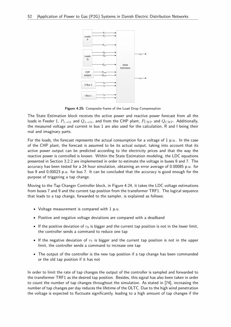
52 Application of Power to Gas (P2G) Systems in Danish Electric Distribution Networks
State Estimator
Loads P
P1P3...
P11
Loads Q
Q1
Q3...
Q11
PCHPQCHP
CHP output
vRviV Bus 1
iRii
I Bus 1
v9
v7
Figure 4.25: Composite frame of the Load Drop Compensation
The State Estimation block receives the active power and reactive power forecast from all theloads in Feeder 1, P1→11 and Q1→11, and from the CHP plant, PCHP and QCHP . Additionally,the measured voltage and current in bus 1 are also used for the calculation, R and I being theirreal and imaginary parts.
For the loads, the forecast represents the actual consumption for a voltage of 1 p.u.. In the caseof the CHP plant, the forecast is assumed to be its actual output, taking into account that itsactive power output can be predicted according to the electricity prices and that the way thereactive power is controlled is known. Within the State Estimation modeling, the LDC equationspresented in Section 3.2.2 are implemented in order to estimate the voltage in buses 9 and 7. Theaccuracy has been tested for a 24 hour simulation, obtaining an error average of 0.00085 p.u. forbus 9 and 0.00023 p.u. for bus 7. It can be concluded that the accuracy is good enough for thepurpose of triggering a tap change.
Moving to the Tap Changer Controller block, in Figure 4.24, it takes the LDC voltage estimationsfrom buses 7 and 9 and the current tap position from the transformer TRF1. The logical sequencethat leads to a tap change, forwarded to the sampler, is explained as follows:
• Voltage measurement is compared with 1 p.u.
• Positive and negative voltage deviations are compared with a deadband
• If the positive deviation of v9 is bigger and the current tap position is not in the lower limit,the controller sends a command to reduce one tap
• If the negative deviation of v7 is bigger and the current tap position is not in the upperlimit, the controller sends a command to increase one tap
• The output of the controller is the new tap position if a tap change has been commandedor the old tap position if it has not
In order to limit the rate of tap changes the output of the controller is sampled and forwarded tothe transformer TRF1 as the desired tap position. Besides, this signal has also been taken in orderto count the number of tap changes throughout the simulation. As stated in [74], increasing thenumber of tap changes per day reduces the lifetime of the OLTC. Due to the high wind penetrationthe voltage is expected to fluctuate significantly, leading to a high amount of tap changes if the
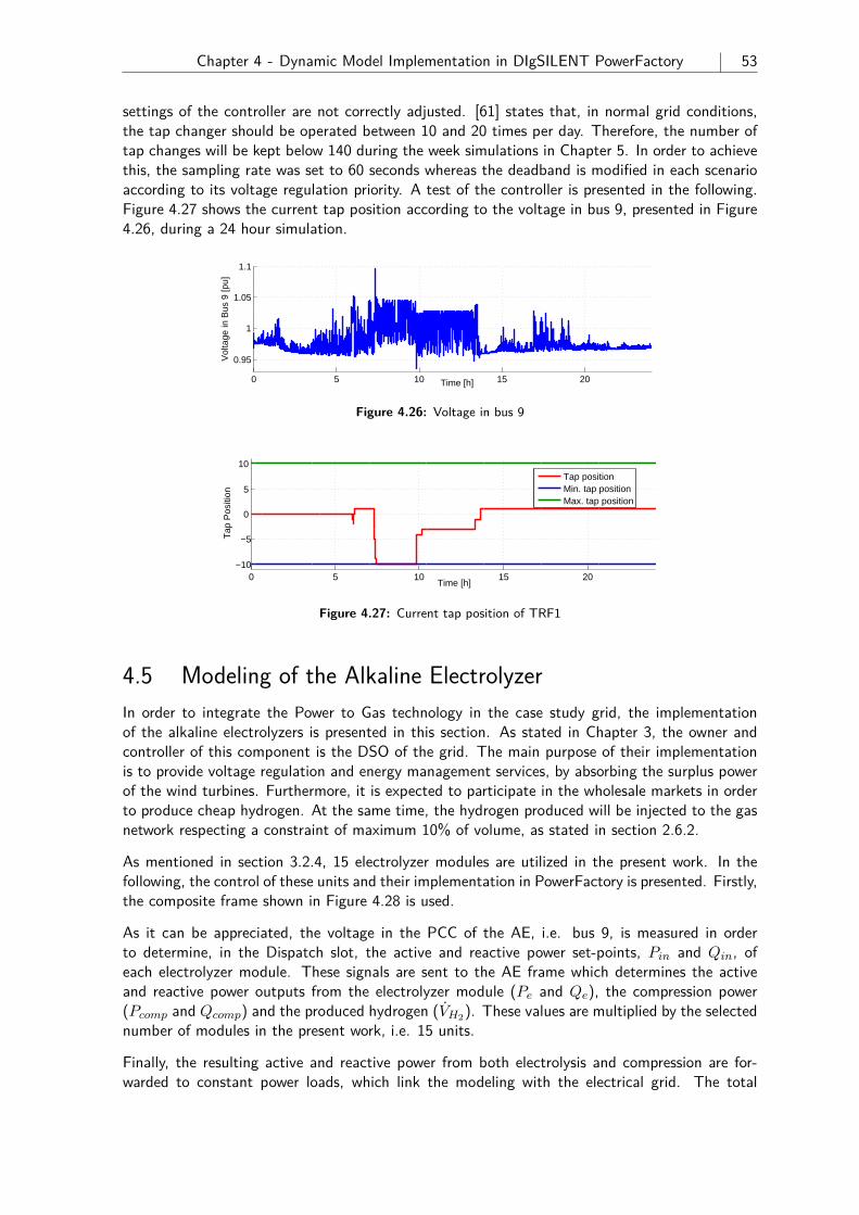
Chapter 4 - Dynamic Model Implementation in DIgSILENT PowerFactory 53
settings of the controller are not correctly adjusted. [61] states that, in normal grid conditions,the tap changer should be operated between 10 and 20 times per day. Therefore, the number oftap changes will be kept below 140 during the week simulations in Chapter 5. In order to achievethis, the sampling rate was set to 60 seconds whereas the deadband is modified in each scenarioaccording to its voltage regulation priority. A test of the controller is presented in the following.Figure 4.27 shows the current tap position according to the voltage in bus 9, presented in Figure4.26, during a 24 hour simulation.
0 5 10 15 20
0.95
1
1.05
1.1
Time [h]
Vol
tage
in B
us 9
[pu]
0 5 10 15 20−10
−5
Time [h]
Figure 4.26: Voltage in bus 9
1.05
1.1
0 5 10 15 20−10
−5
0
5
10
Time [h]
Tap
Pos
ition
Tap positionMin. tap positionMax. tap position
Figure 4.27: Current tap position of TRF1
4.5 Modeling of the Alkaline ElectrolyzerIn order to integrate the Power to Gas technology in the case study grid, the implementationof the alkaline electrolyzers is presented in this section. As stated in Chapter 3, the owner andcontroller of this component is the DSO of the grid. The main purpose of their implementationis to provide voltage regulation and energy management services, by absorbing the surplus powerof the wind turbines. Furthermore, it is expected to participate in the wholesale markets in orderto produce cheap hydrogen. At the same time, the hydrogen produced will be injected to the gasnetwork respecting a constraint of maximum 10% of volume, as stated in section 2.6.2.
As mentioned in section 3.2.4, 15 electrolyzer modules are utilized in the present work. In thefollowing, the control of these units and their implementation in PowerFactory is presented. Firstly,the composite frame shown in Figure 4.28 is used.
As it can be appreciated, the voltage in the PCC of the AE, i.e. bus 9, is measured in orderto determine, in the Dispatch slot, the active and reactive power set-points, Pin and Qin, ofeach electrolyzer module. These signals are sent to the AE frame which determines the activeand reactive power outputs from the electrolyzer module (Pe and Qe), the compression power(Pcomp and Qcomp) and the produced hydrogen (VH2). These values are multiplied by the selectednumber of modules in the present work, i.e. 15 units.
Finally, the resulting active and reactive power from both electrolysis and compression are for-warded to constant power loads, which link the modeling with the electrical grid. The total
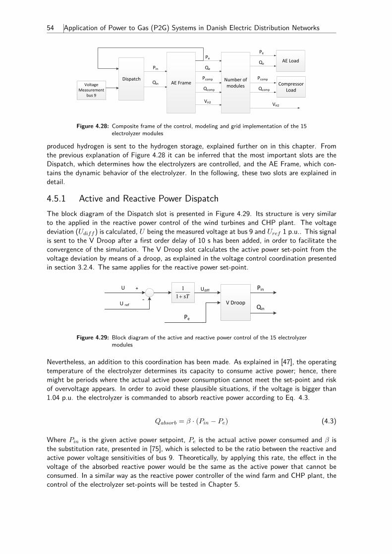
54 Application of Power to Gas (P2G) Systems in Danish Electric Distribution Networks
Pcomp
Qcomp
Dispatch
AE Load
Pin
QinVoltage Measurement
bus 9
Pe
AE Frame
Qe
Number of modules
Qe
VH2 VH2
Pe
Pcomp
Qcomp
CompressorLoad
Figure 4.28: Composite frame of the control, modeling and grid implementation of the 15electrolyzer modules
produced hydrogen is sent to the hydrogen storage, explained further on in this chapter. Fromthe previous explanation of Figure 4.28 it can be inferred that the most important slots are theDispatch, which determines how the electrolyzers are controlled, and the AE Frame, which con-tains the dynamic behavior of the electrolyzer. In the following, these two slots are explained indetail.
4.5.1 Active and Reactive Power DispatchThe block diagram of the Dispatch slot is presented in Figure 4.29. Its structure is very similarto the applied in the reactive power control of the wind turbines and CHP plant. The voltagedeviation (Udiff ) is calculated, U being the measured voltage at bus 9 and Uref 1 p.u.. This signalis sent to the V Droop after a first order delay of 10 s has been added, in order to facilitate theconvergence of the simulation. The V Droop slot calculates the active power set-point from thevoltage deviation by means of a droop, as explained in the voltage control coordination presentedin section 3.2.4. The same applies for the reactive power set-point.
U ref‐
+U Pin
Qin
11 sT
V Droop
Pe
Udiff
Figure 4.29: Block diagram of the active and reactive power control of the 15 electrolyzermodules
Nevertheless, an addition to this coordination has been made. As explained in [47], the operatingtemperature of the electrolyzer determines its capacity to consume active power; hence, theremight be periods where the actual active power consumption cannot meet the set-point and riskof overvoltage appears. In order to avoid these plausible situations, if the voltage is bigger than1.04 p.u. the electrolyzer is commanded to absorb reactive power according to Eq. 4.3.
Qabsorb = β · (Pin − Pe) (4.3)
Where Pin is the given active power setpoint, Pe is the actual active power consumed and β isthe substitution rate, presented in [75], which is selected to be the ratio between the reactive andactive power voltage sensitivities of bus 9. Theoretically, by applying this rate, the effect in thevoltage of the absorbed reactive power would be the same as the active power that cannot beconsumed. In a similar way as the reactive power controller of the wind farm and CHP plant, thecontrol of the electrolyzer set-points will be tested in Chapter 5.
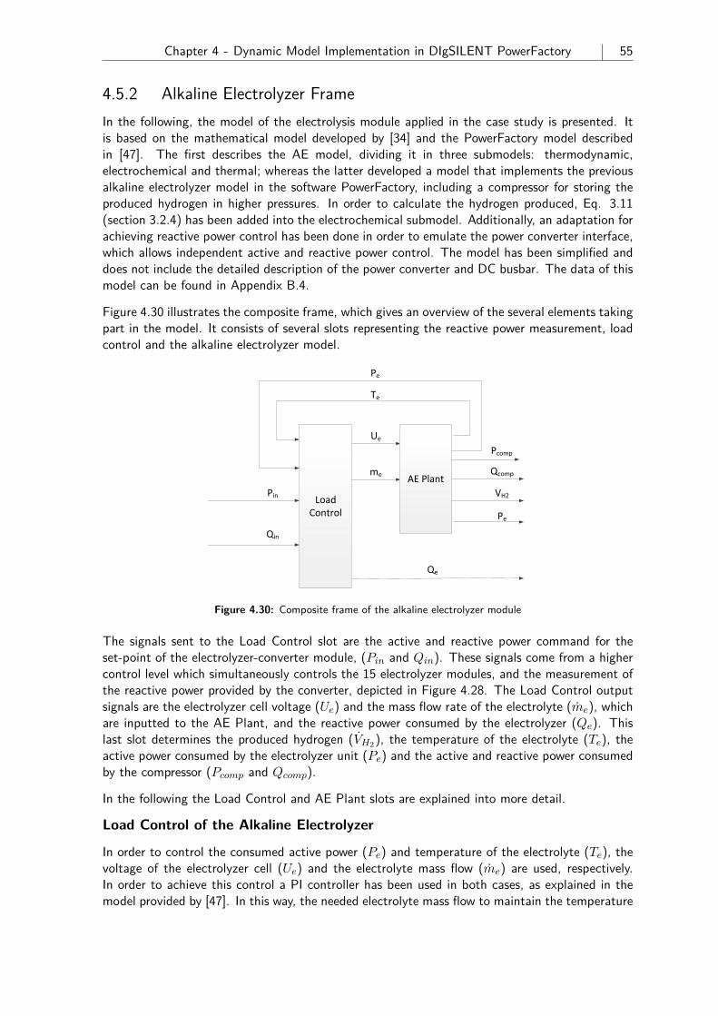
Chapter 4 - Dynamic Model Implementation in DIgSILENT PowerFactory 55
4.5.2 Alkaline Electrolyzer FrameIn the following, the model of the electrolysis module applied in the case study is presented. Itis based on the mathematical model developed by [34] and the PowerFactory model describedin [47]. The first describes the AE model, dividing it in three submodels: thermodynamic,electrochemical and thermal; whereas the latter developed a model that implements the previousalkaline electrolyzer model in the software PowerFactory, including a compressor for storing theproduced hydrogen in higher pressures. In order to calculate the hydrogen produced, Eq. 3.11(section 3.2.4) has been added into the electrochemical submodel. Additionally, an adaptation forachieving reactive power control has been done in order to emulate the power converter interface,which allows independent active and reactive power control. The model has been simplified anddoes not include the detailed description of the power converter and DC busbar. The data of thismodel can be found in Appendix B.4.
Figure 4.30 illustrates the composite frame, which gives an overview of the several elements takingpart in the model. It consists of several slots representing the reactive power measurement, loadcontrol and the alkaline electrolyzer model.
Ue
me
Te
Pe
Pcomp
Qcomp
Load Control
AE Plant
Pin
Qin
Qe
Pe
VH2
Figure 4.30: Composite frame of the alkaline electrolyzer module
The signals sent to the Load Control slot are the active and reactive power command for theset-point of the electrolyzer-converter module, (Pin and Qin). These signals come from a highercontrol level which simultaneously controls the 15 electrolyzer modules, and the measurement ofthe reactive power provided by the converter, depicted in Figure 4.28. The Load Control outputsignals are the electrolyzer cell voltage (Ue) and the mass flow rate of the electrolyte (me), whichare inputted to the AE Plant, and the reactive power consumed by the electrolyzer (Qe). Thislast slot determines the produced hydrogen (VH2), the temperature of the electrolyte (Te), theactive power consumed by the electrolyzer unit (Pe) and the active and reactive power consumedby the compressor (Pcomp and Qcomp).
In the following the Load Control and AE Plant slots are explained into more detail.
Load Control of the Alkaline Electrolyzer
In order to control the consumed active power (Pe) and temperature of the electrolyte (Te), thevoltage of the electrolyzer cell (Ue) and the electrolyte mass flow (me) are used, respectively.In order to achieve this control a PI controller has been used in both cases, as explained in themodel provided by [47]. In this way, the needed electrolyte mass flow to maintain the temperature
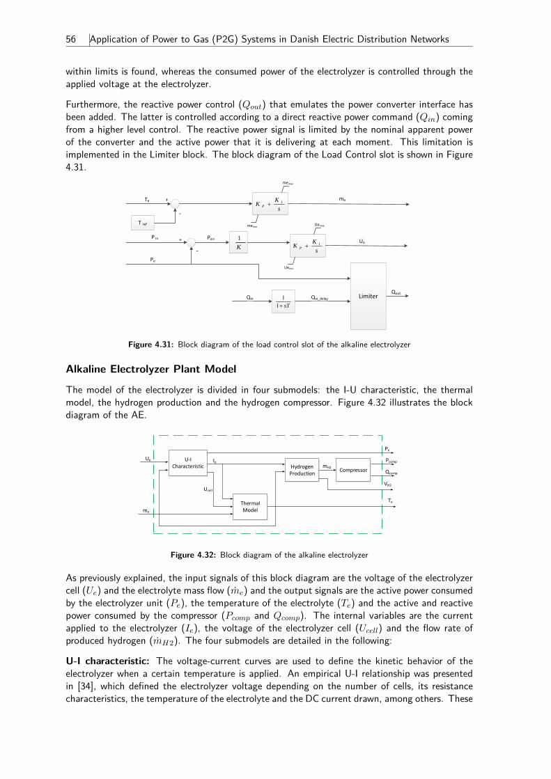
56 Application of Power to Gas (P2G) Systems in Danish Electric Distribution Networks
within limits is found, whereas the consumed power of the electrolyzer is controlled through theapplied voltage at the electrolyzer.
Furthermore, the reactive power control (Qout) that emulates the power converter interface hasbeen added. The latter is controlled according to a direct reactive power command (Qin) comingfrom a higher level control. The reactive power signal is limited by the nominal apparent powerof the converter and the active power that it is delivering at each moment. This limitation isimplemented in the Limiter block. The block diagram of the Load Control slot is shown in Figure4.31.
Perr
Pe
‐
+P in
Uemax
Uemin
sK
K IP K
1
‐
+Te
T ref
memax
memin
sK
K IP
me
Qin
Ue
LimiterQin_delay
Qout
11 sT
Figure 4.31: Block diagram of the load control slot of the alkaline electrolyzer
Alkaline Electrolyzer Plant Model
The model of the electrolyzer is divided in four submodels: the I-U characteristic, the thermalmodel, the hydrogen production and the hydrogen compressor. Figure 4.32 illustrates the blockdiagram of the AE.
Ie
me
Ue
Ucell
Pe
mH2
Te
Pcomp
Qcomp
Ue
me
Te
Pe
Pcomp
Qcomp
Pext
Qext
U-I Characteristic
Thermal Model
Hydrogen Production
CompressorLoad Control
Power Signal
AE PlantPQ
LoadAE
Load
VH2
Figure 4.32: Block diagram of the alkaline electrolyzer
As previously explained, the input signals of this block diagram are the voltage of the electrolyzercell (Ue) and the electrolyte mass flow (me) and the output signals are the active power consumedby the electrolyzer unit (Pe), the temperature of the electrolyte (Te) and the active and reactivepower consumed by the compressor (Pcomp and Qcomp). The internal variables are the currentapplied to the electrolyzer (Ie), the voltage of the electrolyzer cell (Ucell) and the flow rate ofproduced hydrogen (mH2). The four submodels are detailed in the following:
U-I characteristic: The voltage-current curves are used to define the kinetic behavior of theelectrolyzer when a certain temperature is applied. An empirical U-I relationship was presentedin [34], which defined the electrolyzer voltage depending on the number of cells, its resistancecharacteristics, the temperature of the electrolyte and the DC current drawn, among others. These
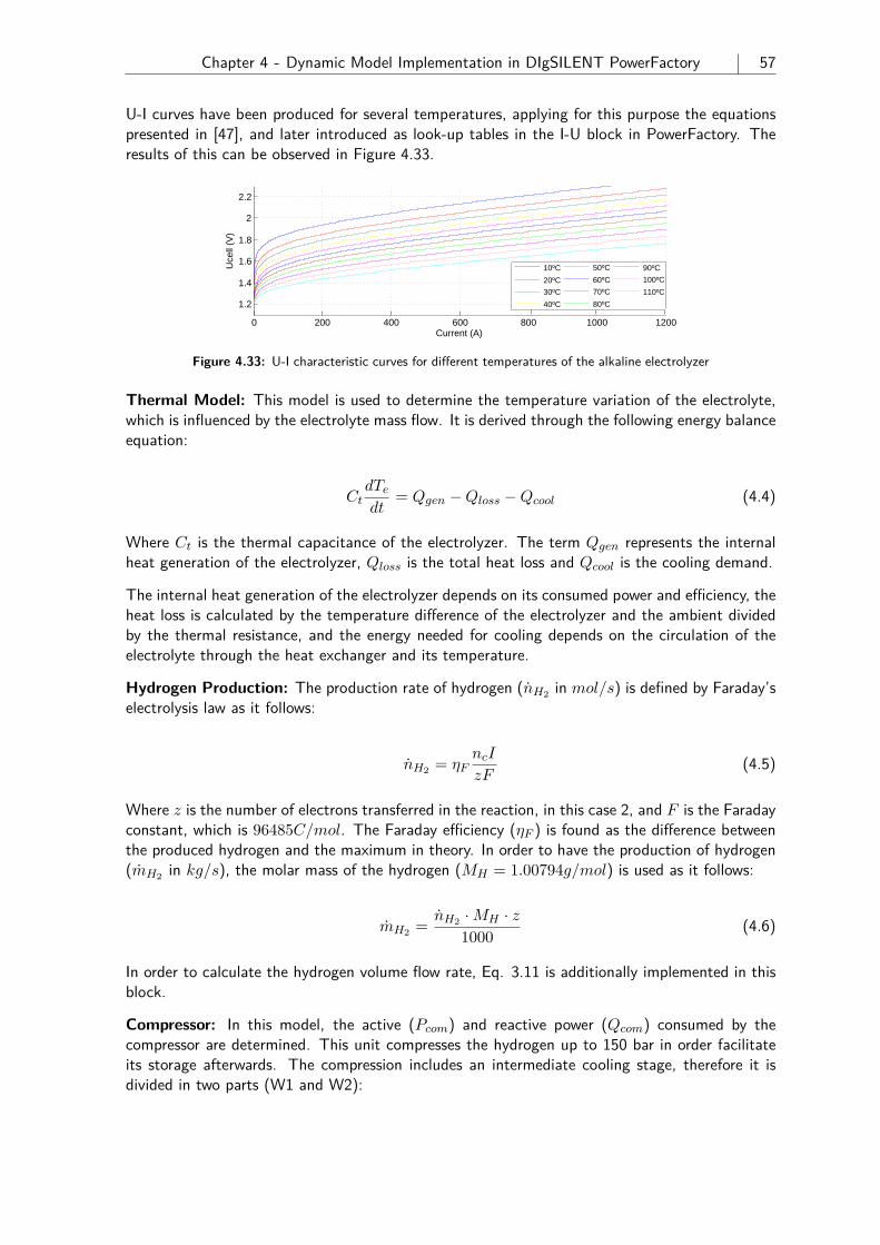
Chapter 4 - Dynamic Model Implementation in DIgSILENT PowerFactory 57
U-I curves have been produced for several temperatures, applying for this purpose the equationspresented in [47], and later introduced as look-up tables in the I-U block in PowerFactory. Theresults of this can be observed in Figure 4.33.
0 200 400 600 800 1000 1200
1.2
1.4
1.6
1.8
2
2.2
Current (A)
Uce
ll (V
)
10ºC
20ºC
30ºC
40ºC
50ºC
60ºC70ºC
80ºC
90ºC
100ºC
110ºC
Figure 4.33: U-I characteristic curves for different temperatures of the alkaline electrolyzer
Thermal Model: This model is used to determine the temperature variation of the electrolyte,which is influenced by the electrolyte mass flow. It is derived through the following energy balanceequation:
CtdTedt
= Qgen −Qloss −Qcool (4.4)
Where Ct is the thermal capacitance of the electrolyzer. The term Qgen represents the internalheat generation of the electrolyzer, Qloss is the total heat loss and Qcool is the cooling demand.
The internal heat generation of the electrolyzer depends on its consumed power and efficiency, theheat loss is calculated by the temperature difference of the electrolyzer and the ambient dividedby the thermal resistance, and the energy needed for cooling depends on the circulation of theelectrolyte through the heat exchanger and its temperature.
Hydrogen Production: The production rate of hydrogen (nH2 in mol/s) is defined by Faraday’selectrolysis law as it follows:
nH2 = ηFncI
zF(4.5)
Where z is the number of electrons transferred in the reaction, in this case 2, and F is the Faradayconstant, which is 96485C/mol. The Faraday efficiency (ηF ) is found as the difference betweenthe produced hydrogen and the maximum in theory. In order to have the production of hydrogen(mH2 in kg/s), the molar mass of the hydrogen (MH = 1.00794g/mol) is used as it follows:
mH2 = nH2 ·MH · z1000 (4.6)
In order to calculate the hydrogen volume flow rate, Eq. 3.11 is additionally implemented in thisblock.
Compressor: In this model, the active (Pcom) and reactive power (Qcom) consumed by thecompressor are determined. This unit compresses the hydrogen up to 150 bar in order facilitateits storage afterwards. The compression includes an intermediate cooling stage, therefore it isdivided in two parts (W1 and W2):
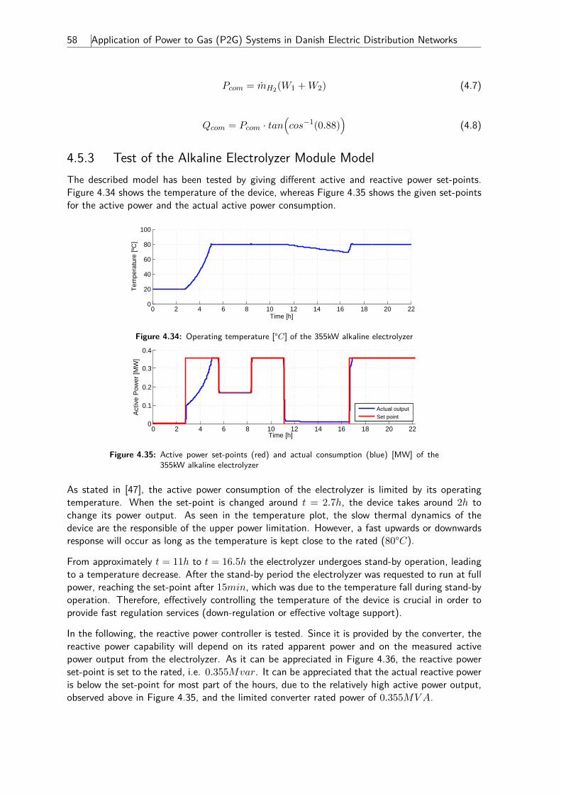
58 Application of Power to Gas (P2G) Systems in Danish Electric Distribution Networks
Pcom = mH2(W1 +W2) (4.7)
Qcom = Pcom · tan(cos−1(0.88)
)(4.8)
4.5.3 Test of the Alkaline Electrolyzer Module ModelThe described model has been tested by giving different active and reactive power set-points.Figure 4.34 shows the temperature of the device, whereas Figure 4.35 shows the given set-pointsfor the active power and the actual active power consumption.
0 2 4 6 8 10 12 14 16 18 20 220
20
40
60
80
100
Time [h]
Tem
pera
ture
[ºC
]
Figure 4.34: Operating temperature [°C] of the 355kW alkaline electrolyzer
0 2 4 6 8 10 12 14 16 18 20 220
0.1
0.2
0.3
0.4
Time [h]
Act
ive
Pow
er [M
W]
Actual output Set point
Figure 4.35: Active power set-points (red) and actual consumption (blue) [MW] of the355kW alkaline electrolyzer
As stated in [47], the active power consumption of the electrolyzer is limited by its operatingtemperature. When the set-point is changed around t = 2.7h, the device takes around 2h tochange its power output. As seen in the temperature plot, the slow thermal dynamics of thedevice are the responsible of the upper power limitation. However, a fast upwards or downwardsresponse will occur as long as the temperature is kept close to the rated (80°C).
From approximately t = 11h to t = 16.5h the electrolyzer undergoes stand-by operation, leadingto a temperature decrease. After the stand-by period the electrolyzer was requested to run at fullpower, reaching the set-point after 15min, which was due to the temperature fall during stand-byoperation. Therefore, effectively controlling the temperature of the device is crucial in order toprovide fast regulation services (down-regulation or effective voltage support).
In the following, the reactive power controller is tested. Since it is provided by the converter, thereactive power capability will depend on its rated apparent power and on the measured activepower output from the electrolyzer. As it can be appreciated in Figure 4.36, the reactive powerset-point is set to the rated, i.e. 0.355Mvar. It can be appreciated that the actual reactive poweris below the set-point for most part of the hours, due to the relatively high active power output,observed above in Figure 4.35, and the limited converter rated power of 0.355MVA.
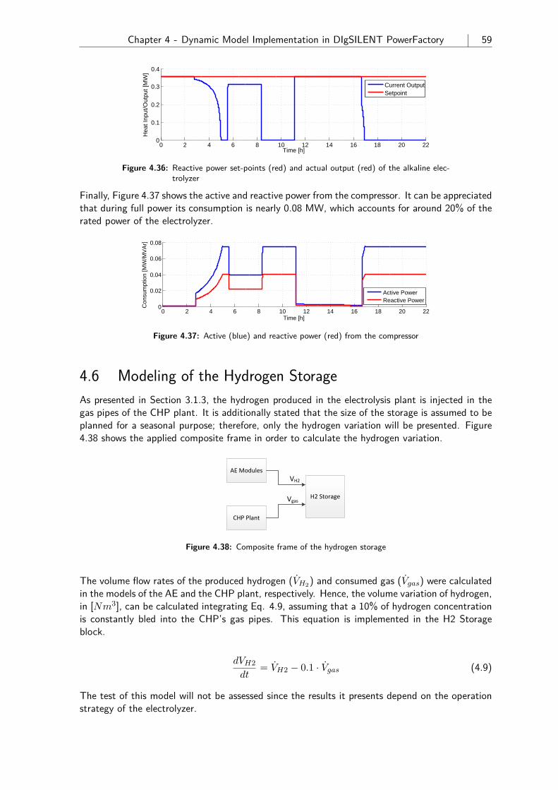
Chapter 4 - Dynamic Model Implementation in DIgSILENT PowerFactory 59
0 2 4 6 8 10 12 14 16 18 20 220
0.1
0.2
0.3
0.4
Time [h]H
eat I
nput
/Out
put [
MW
]
Current OutputSetpoint
Figure 4.36: Reactive power set-points (red) and actual output (red) of the alkaline elec-trolyzer
Finally, Figure 4.37 shows the active and reactive power from the compressor. It can be appreciatedthat during full power its consumption is nearly 0.08 MW, which accounts for around 20% of therated power of the electrolyzer.
0 2 4 6 8 10 12 14 16 18 20 220
0.02
0.04
0.06
0.08
Time [h]
Con
sum
ptio
n [M
W/M
VA
r]
Active PowerReactive Power
Figure 4.37: Active (blue) and reactive power (red) from the compressor
4.6 Modeling of the Hydrogen StorageAs presented in Section 3.1.3, the hydrogen produced in the electrolysis plant is injected in thegas pipes of the CHP plant. It is additionally stated that the size of the storage is assumed to beplanned for a seasonal purpose; therefore, only the hydrogen variation will be presented. Figure4.38 shows the applied composite frame in order to calculate the hydrogen variation.
AE Modules
CHP Plant
H2 Storage
VH2
Vgas
Figure 4.38: Composite frame of the hydrogen storage
The volume flow rates of the produced hydrogen (VH2) and consumed gas (Vgas) were calculatedin the models of the AE and the CHP plant, respectively. Hence, the volume variation of hydrogen,in [Nm3], can be calculated integrating Eq. 4.9, assuming that a 10% of hydrogen concentrationis constantly bled into the CHP’s gas pipes. This equation is implemented in the H2 Storageblock.
dVH2dt
= VH2 − 0.1 · Vgas (4.9)
The test of this model will not be assessed since the results it presents depend on the operationstrategy of the electrolyzer.
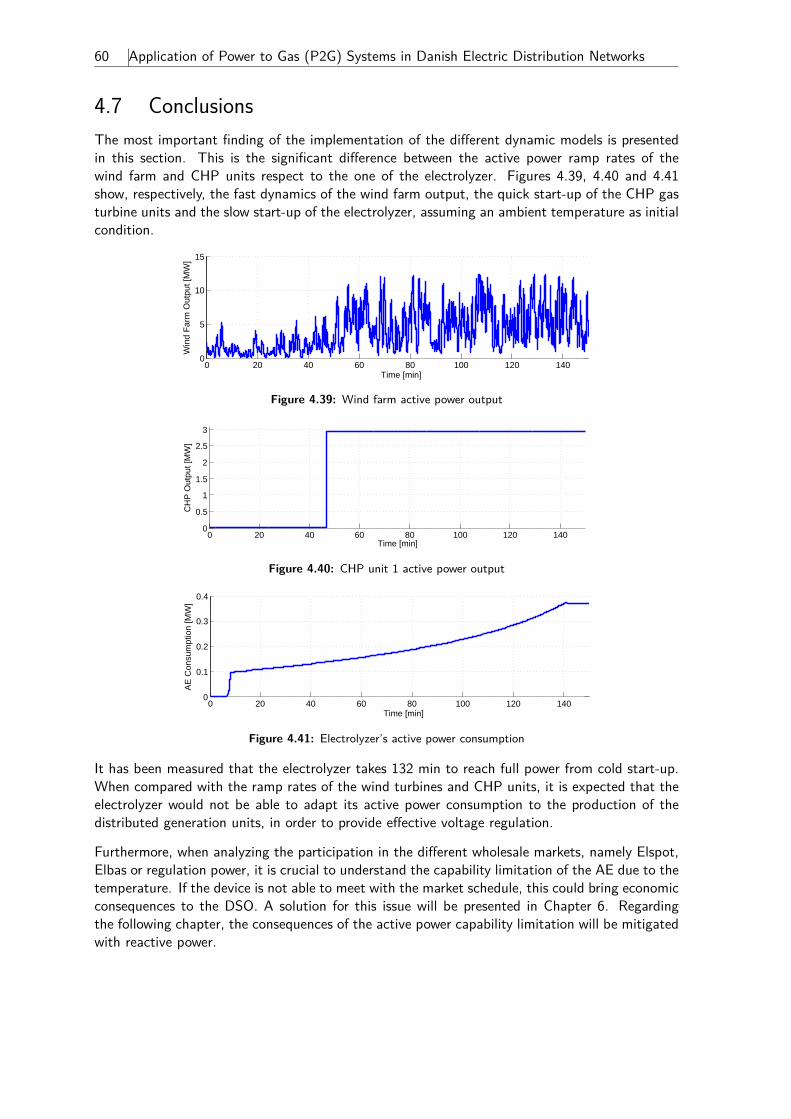
60 Application of Power to Gas (P2G) Systems in Danish Electric Distribution Networks
4.7 ConclusionsThe most important finding of the implementation of the different dynamic models is presentedin this section. This is the significant difference between the active power ramp rates of thewind farm and CHP units respect to the one of the electrolyzer. Figures 4.39, 4.40 and 4.41show, respectively, the fast dynamics of the wind farm output, the quick start-up of the CHP gasturbine units and the slow start-up of the electrolyzer, assuming an ambient temperature as initialcondition.
0 20 40 60 80 100 120 1400
5
10
15
Time [min]
Win
d F
arm
Out
put [
MW
]
Figure 4.39: Wind farm active power output
0 20 40 60 80 100 120 1400
0.5
1
1.5
2
2.5
3
Time [min]
CH
P O
utpu
t [M
W]
Figure 4.40: CHP unit 1 active power output
0 20 40 60 80 100 120 1400
0.1
0.2
0.3
0.4
Time [min]
AE
Con
sum
ptio
n [M
W]
Figure 4.41: Electrolyzer’s active power consumption
It has been measured that the electrolyzer takes 132 min to reach full power from cold start-up.When compared with the ramp rates of the wind turbines and CHP units, it is expected that theelectrolyzer would not be able to adapt its active power consumption to the production of thedistributed generation units, in order to provide effective voltage regulation.
Furthermore, when analyzing the participation in the different wholesale markets, namely Elspot,Elbas or regulation power, it is crucial to understand the capability limitation of the AE due to thetemperature. If the device is not able to meet with the market schedule, this could bring economicconsequences to the DSO. A solution for this issue will be presented in Chapter 6. Regardingthe following chapter, the consequences of the active power capability limitation will be mitigatedwith reactive power.
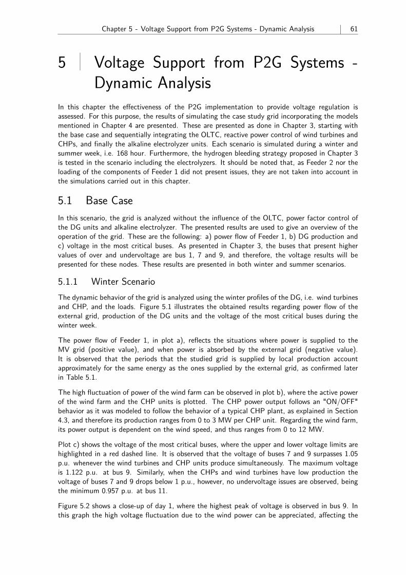
Chapter 5 - Voltage Support from P2G Systems - Dynamic Analysis 61
5 Voltage Support from P2G Systems -Dynamic Analysis
In this chapter the effectiveness of the P2G implementation to provide voltage regulation isassessed. For this purpose, the results of simulating the case study grid incorporating the modelsmentioned in Chapter 4 are presented. These are presented as done in Chapter 3, starting withthe base case and sequentially integrating the OLTC, reactive power control of wind turbines andCHPs, and finally the alkaline electrolyzer units. Each scenario is simulated during a winter andsummer week, i.e. 168 hour. Furthermore, the hydrogen bleeding strategy proposed in Chapter 3is tested in the scenario including the electrolyzers. It should be noted that, as Feeder 2 nor theloading of the components of Feeder 1 did not present issues, they are not taken into account inthe simulations carried out in this chapter.
5.1 Base CaseIn this scenario, the grid is analyzed without the influence of the OLTC, power factor control ofthe DG units and alkaline electrolyzer. The presented results are used to give an overview of theoperation of the grid. These are the following: a) power flow of Feeder 1, b) DG production andc) voltage in the most critical buses. As presented in Chapter 3, the buses that present highervalues of over and undervoltage are bus 1, 7 and 9, and therefore, the voltage results will bepresented for these nodes. These results are presented in both winter and summer scenarios.
5.1.1 Winter ScenarioThe dynamic behavior of the grid is analyzed using the winter profiles of the DG, i.e. wind turbinesand CHP, and the loads. Figure 5.1 illustrates the obtained results regarding power flow of theexternal grid, production of the DG units and the voltage of the most critical buses during thewinter week.
The power flow of Feeder 1, in plot a), reflects the situations where power is supplied to theMV grid (positive value), and when power is absorbed by the external grid (negative value).It is observed that the periods that the studied grid is supplied by local production accountapproximately for the same energy as the ones supplied by the external grid, as confirmed laterin Table 5.1.
The high fluctuation of power of the wind farm can be observed in plot b), where the active powerof the wind farm and the CHP units is plotted. The CHP power output follows an "ON/OFF"behavior as it was modeled to follow the behavior of a typical CHP plant, as explained in Section4.3, and therefore its production ranges from 0 to 3 MW per CHP unit. Regarding the wind farm,its power output is dependent on the wind speed, and thus ranges from 0 to 12 MW.
Plot c) shows the voltage of the most critical buses, where the upper and lower voltage limits arehighlighted in a red dashed line. It is observed that the voltage of buses 7 and 9 surpasses 1.05p.u. whenever the wind turbines and CHP units produce simultaneously. The maximum voltageis 1.122 p.u. at bus 9. Similarly, when the CHPs and wind turbines have low production thevoltage of buses 7 and 9 drops below 1 p.u., however, no undervoltage issues are observed, beingthe minimum 0.957 p.u. at bus 11.
Figure 5.2 shows a close-up of day 1, where the highest peak of voltage is observed in bus 9. Inthis graph the high voltage fluctuation due to the wind power can be appreciated, affecting the
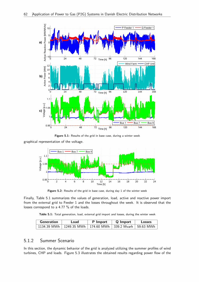
62 Application of Power to Gas (P2G) Systems in Danish Electric Distribution Networks
0 24 48 72 96 120 144 1680
2
4
6
8
10
12
Time [h]
Act
ive
Pow
er [M
W]
Wind Farm CHP Unit
c)
0 24 48 72 96 120 144 168
1
1.05
1.1
Time [h]
Volta
ge [p
.u.]
0.95 Bus 1 Bus 7 Bus 9
a)
0 24 48 72 96 120 144 168
−5
0
5
10
Time [h]Activ
e/ R
eact
ive
Pow
er [M
W/M
VAr]
−10
P Feeder 1 Q Feeder 1
b)
Figure 5.1: Results of the grid in base case, during a winter week
graphical representation of the voltage.
0 2 4 6 8 10 12 14 16 18 20 22 240.95
1
1.05
1.1
Time [h]
Vol
tage
[p.u
.]
Bus 1 Bus 7 Bus 9
Figure 5.2: Results of the grid in base case, during day 1 of the winter week
Finally, Table 5.1 summarizes the values of generation, load, active and reactive power importfrom the external grid to Feeder 1 and the losses throughout the week. It is observed that thelosses correspond to a 4.77 % of the loads.
Table 5.1: Total generation, load, external grid import and losses, during the winter week
Generation Load P Import Q Import Losses1134.39 MWh 1249.35 MWh 174.60 MWh 339.2 Mvarh 59.63 MWh
5.1.2 Summer ScenarioIn this section, the dynamic behavior of the grid is analyzed utilizing the summer profiles of windturbines, CHP and loads. Figure 5.3 illustrates the obtained results regarding power flow of the
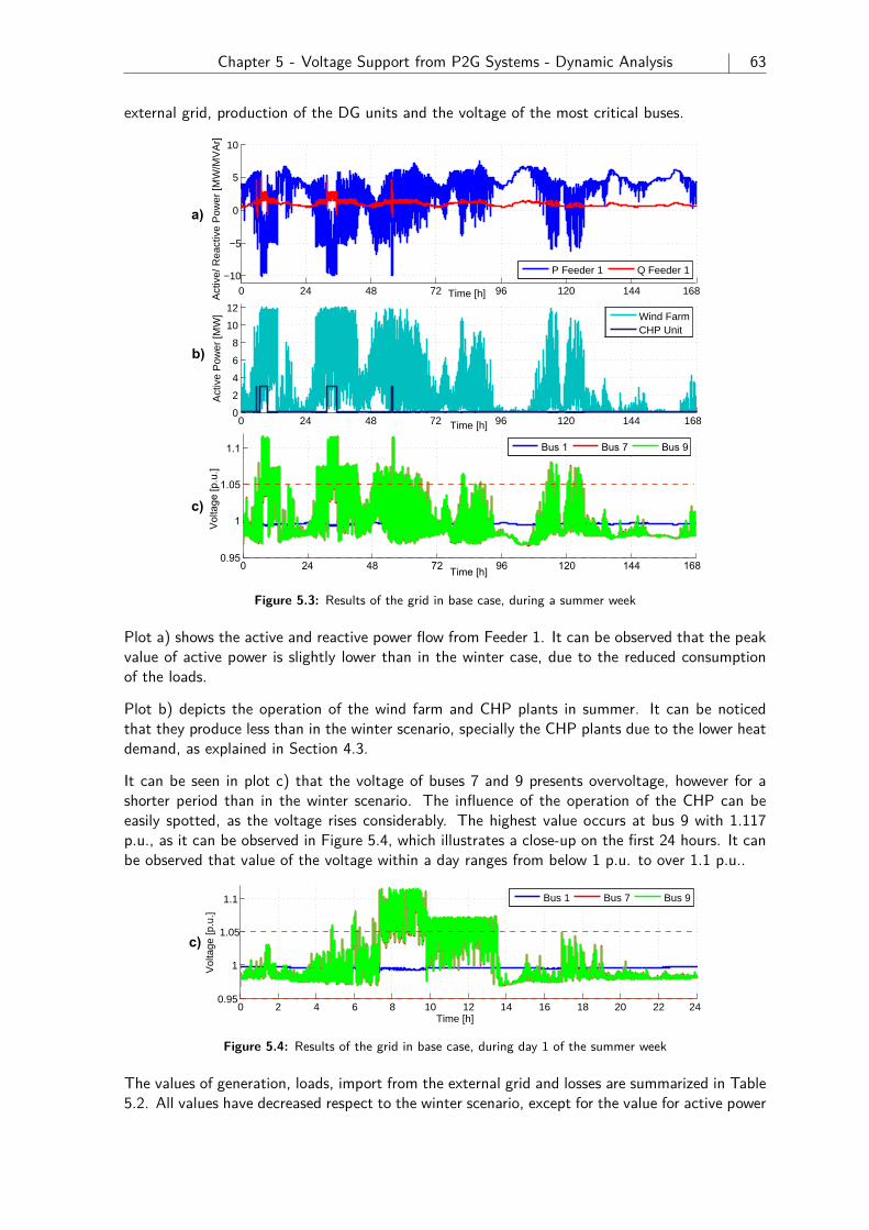
Chapter 5 - Voltage Support from P2G Systems - Dynamic Analysis 63
external grid, production of the DG units and the voltage of the most critical buses.
a)
c)
b)
0 24 48 72 96 120 144 168
1
1.05
1.1
Time [h]
Volta
ge [p
.u.]
0.95
Bus 1 Bus 7 Bus 9
0 24 48 72 96 120 144 168−10
−5
0
5
10
Time [h]Act
ive/
Rea
ctiv
e P
ower
[MW
/MV
Ar]
P Feeder 1 Q Feeder 1
0 24 48 72 96 120 144 168
2
4
6
8
10
12
Time [h]
Act
ive
Pow
er [M
W]
0
Wind FarmCHP Unit
Figure 5.3: Results of the grid in base case, during a summer week
Plot a) shows the active and reactive power flow from Feeder 1. It can be observed that the peakvalue of active power is slightly lower than in the winter case, due to the reduced consumptionof the loads.
Plot b) depicts the operation of the wind farm and CHP plants in summer. It can be noticedthat they produce less than in the winter scenario, specially the CHP plants due to the lower heatdemand, as explained in Section 4.3.
It can be seen in plot c) that the voltage of buses 7 and 9 presents overvoltage, however for ashorter period than in the winter scenario. The influence of the operation of the CHP can beeasily spotted, as the voltage rises considerably. The highest value occurs at bus 9 with 1.117p.u., as it can be observed in Figure 5.4, which illustrates a close-up on the first 24 hours. It canbe observed that value of the voltage within a day ranges from below 1 p.u. to over 1.1 p.u..
0 2 4 6 8 10 12 14 16 18 20 22 240.95
1
1.05
1.1
Time [h]
Vol
tage
[p.u
.]
Bus 1 Bus 7 Bus 9
c)
Figure 5.4: Results of the grid in base case, during day 1 of the summer week
The values of generation, loads, import from the external grid and losses are summarized in Table5.2. All values have decreased respect to the winter scenario, except for the value for active power
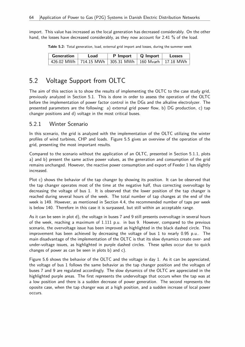
64 Application of Power to Gas (P2G) Systems in Danish Electric Distribution Networks
import. This value has increased as the local generation has decreased considerably. On the otherhand, the losses have decreased considerably, as they now account for 2.41 % of the load.
Table 5.2: Total generation, load, external grid import and losses, during the summer week
Generation Load P Import Q Import Losses426.02 MWh 714.15 MWh 305.31 MWh 160 Mvarh 17.18 MWh
5.2 Voltage Support from OLTCThe aim of this section is to show the results of implementing the OLTC to the case study grid,previously analyzed in Section 5.1. This is done in order to assess the operation of the OLTCbefore the implementation of power factor control in the DGs and the alkaline electrolyzer. Thepresented parameters are the following: a) external grid power flow, b) DG production, c) tapchanger positions and d) voltage in the most critical buses.
5.2.1 Winter ScenarioIn this scenario, the grid is analyzed with the implementation of the OLTC utilizing the winterprofiles of wind turbines, CHP and loads. Figure 5.5 gives an overview of the operation of thegrid, presenting the most important results.
Compared to the scenario without the application of an OLTC, presented in Section 5.1.1, plotsa) and b) present the same active power values, as the generation and consumption of the gridremains unchanged. However, the reactive power consumption and export of Feeder 1 has slightlyincreased.
Plot c) shows the behavior of the tap changer by showing its position. It can be observed thatthe tap changer operates most of the time at the negative half, thus correcting overvoltage bydecreasing the voltage of bus 1. It is observed that the lower position of the tap changer isreached during several hours of the week. The total number of tap changes at the end of theweek is 149. However, as mentioned in Section 4.4, the recommended number of taps per weekis below 140. Therefore in this case it is surpassed, but still within an acceptable range.
As it can be seen in plot d), the voltage in buses 7 and 9 still presents overvoltage in several hoursof the week, reaching a maximum of 1.111 p.u. in bus 9. However, compared to the previousscenario, the overvoltage issue has been improved as highlighted in the black dashed circle. Thisimprovement has been achieved by decreasing the voltage of bus 1 to nearly 0.95 p.u.. Themain disadvantage of the implementation of the OLTC is that its slow dynamics create over- andunder-voltage issues, as highlighted in purple dashed circles. These spikes occur due to quickchanges of power as can be seen in plots b) and c).
Figure 5.6 shows the behavior of the OLTC and the voltage in day 1. As it can be appreciated,the voltage of bus 1 follows the same behavior as the tap changer position and the voltages ofbuses 7 and 9 are regulated accordingly. The slow dynamics of the OLTC are appreciated in thehighlighted purple areas. The first represents the undervoltage that occurs when the tap was ata low position and there is a sudden decrease of power generation. The second represents theoposite case, when the tap changer was at a high position, and a sudden increase of local poweroccurs.
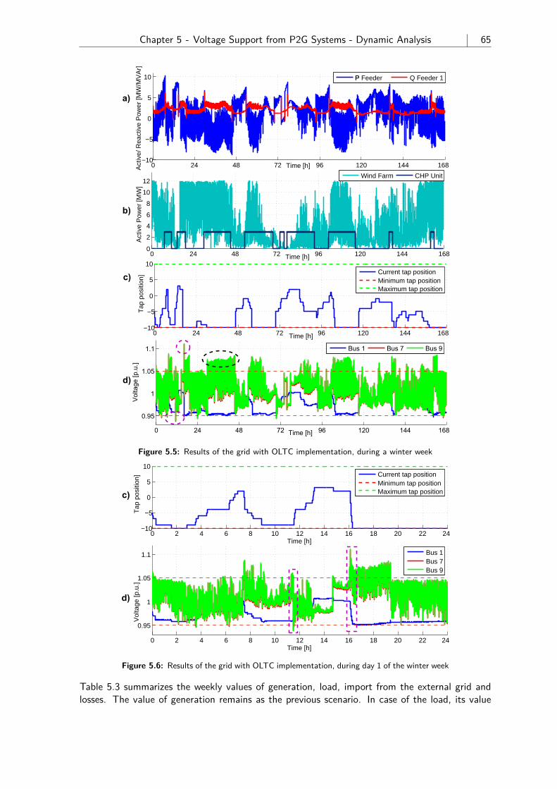
Chapter 5 - Voltage Support from P2G Systems - Dynamic Analysis 65
0 24 48 72 96 120 144 1680
2
4
6
8
10
12
Time [h]
Act
ive
Pow
er [M
W]
Wind Farm CHP Unit
a)
0 24 48 72 96 120 144 168
−5
0
5
10
Time [h]Act
ive/
Rea
ctiv
e P
ower
[MW
/MV
Ar]
−10
PP Feeder Q Feeder 1
c)
d)
0 24 48 72 96 120 144 168
0.95
1
1.05
1.1
Time [h]
Volta
ge [p
.u.]
Bus 1 Bus 7 Bus 9
b)
0 24 48 72 96 120 144 168
−5
0
5
10
Time [h]
Tap
pos
ition
]
−10
Current tap positionMinimum tap positionMaximum tap position
Figure 5.5: Results of the grid with OLTC implementation, during a winter week
0 2 4 6 8 10 12 14 16 18 20 22 24
0.95
1
1.05
1.1
Time [h]
Vol
tage
[p.u
.]
Bus 1Bus 7Bus 9
0 2 4 6 8 10 12 14 16 18 20 22 24
−5
0
5
10
Time [h]
Tap
pos
ition
]
−10
Current tap positionMinimum tap positionMaximum tap positionc)
d)
Figure 5.6: Results of the grid with OLTC implementation, during day 1 of the winter week
Table 5.3 summarizes the weekly values of generation, load, import from the external grid andlosses. The value of generation remains as the previous scenario. In case of the load, its value
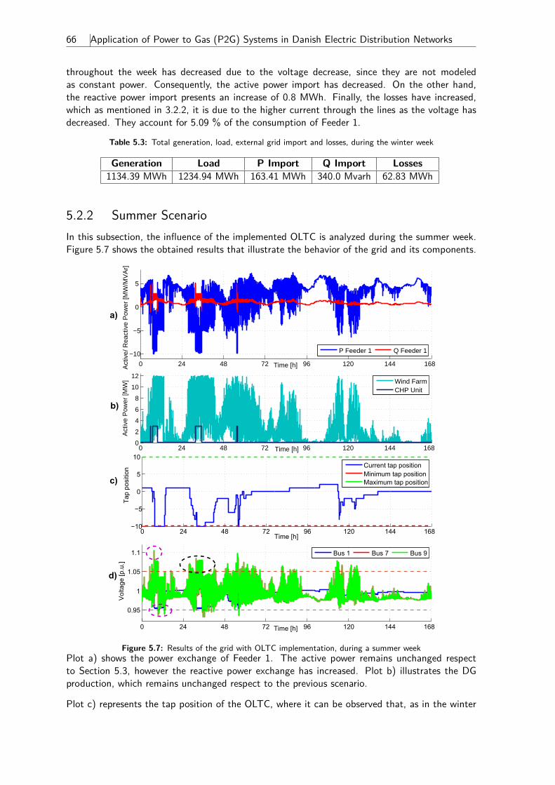
66 Application of Power to Gas (P2G) Systems in Danish Electric Distribution Networks
throughout the week has decreased due to the voltage decrease, since they are not modeledas constant power. Consequently, the active power import has decreased. On the other hand,the reactive power import presents an increase of 0.8 MWh. Finally, the losses have increased,which as mentioned in 3.2.2, it is due to the higher current through the lines as the voltage hasdecreased. They account for 5.09 % of the consumption of Feeder 1.
Table 5.3: Total generation, load, external grid import and losses, during the winter week
Generation Load P Import Q Import Losses1134.39 MWh 1234.94 MWh 163.41 MWh 340.0 Mvarh 62.83 MWh
5.2.2 Summer ScenarioIn this subsection, the influence of the implemented OLTC is analyzed during the summer week.Figure 5.7 shows the obtained results that illustrate the behavior of the grid and its components.
a)
c)
b)
d)
0 24 48 72 96 120 144 168
−5
0
5
10
Time [h]
Tap
posi
tion
−10
Current tap positionMinimum tap positionMaximum tap position
0 24 48 72 96 120 144 168
0.95
1
1.05
1.1
Time [h]
Volta
ge [p
.u.]
Bus 1 Bus 7 Bus 9
0 24 48 72 96 120 144 168
−10
−5
0
5
Time [h]Act
ive/
Rea
ctiv
e P
ower
[MW
/MV
Ar]
P Feeder 1 Q Feeder 1
0 24 48 72 96 120 144 168
2
4
6
8
10
12
Time [h]
Act
ive
Pow
er [M
W]
0
Wind FarmCHP Unit
Figure 5.7: Results of the grid with OLTC implementation, during a summer weekPlot a) shows the power exchange of Feeder 1. The active power remains unchanged respectto Section 5.3, however the reactive power exchange has increased. Plot b) illustrates the DGproduction, which remains unchanged respect to the previous scenario.
Plot c) represents the tap position of the OLTC, where it can be observed that, as in the winter
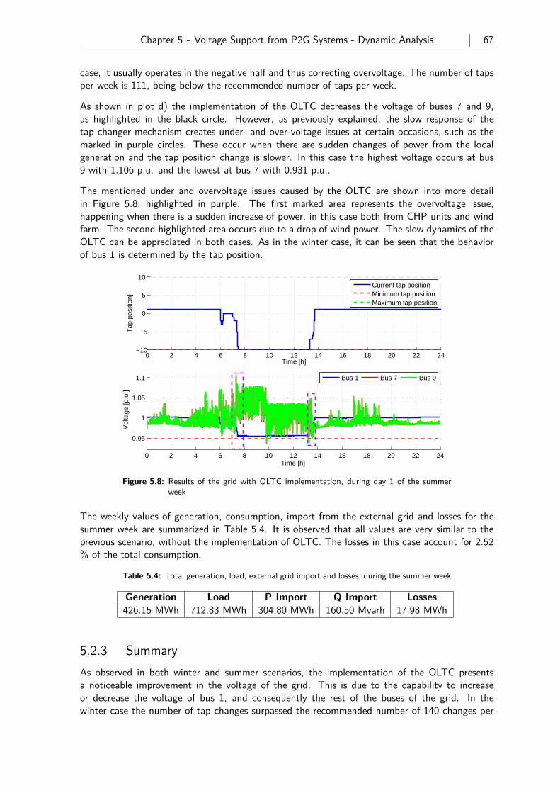
Chapter 5 - Voltage Support from P2G Systems - Dynamic Analysis 67
case, it usually operates in the negative half and thus correcting overvoltage. The number of tapsper week is 111, being below the recommended number of taps per week.
As shown in plot d) the implementation of the OLTC decreases the voltage of buses 7 and 9,as highlighted in the black circle. However, as previously explained, the slow response of thetap changer mechanism creates under- and over-voltage issues at certain occasions, such as themarked in purple circles. These occur when there are sudden changes of power from the localgeneration and the tap position change is slower. In this case the highest voltage occurs at bus9 with 1.106 p.u. and the lowest at bus 7 with 0.931 p.u..
The mentioned under and overvoltage issues caused by the OLTC are shown into more detailin Figure 5.8, highlighted in purple. The first marked area represents the overvoltage issue,happening when there is a sudden increase of power, in this case both from CHP units and windfarm. The second highlighted area occurs due to a drop of wind power. The slow dynamics of theOLTC can be appreciated in both cases. As in the winter case, it can be seen that the behaviorof bus 1 is determined by the tap position.
0 2 4 6 8 10 12 14 16 18 20 22 24−10
−5
0
5
10
Time [h]
Tap
pos
ition
]
Current tap positionMinimum tap positionMaximum tap position
0 2 4 6 8 10 12 14 16 18 20 22 24
0.95
1
1.05
1.1
Time [h]
Vol
tage
[p.u
.]
Bus 1 Bus 7 Bus 9
Figure 5.8: Results of the grid with OLTC implementation, during day 1 of the summerweek
The weekly values of generation, consumption, import from the external grid and losses for thesummer week are summarized in Table 5.4. It is observed that all values are very similar to theprevious scenario, without the implementation of OLTC. The losses in this case account for 2.52% of the total consumption.
Table 5.4: Total generation, load, external grid import and losses, during the summer week
Generation Load P Import Q Import Losses426.15 MWh 712.83 MWh 304.80 MWh 160.50 Mvarh 17.98 MWh
5.2.3 SummaryAs observed in both winter and summer scenarios, the implementation of the OLTC presentsa noticeable improvement in the voltage of the grid. This is due to the capability to increaseor decrease the voltage of bus 1, and consequently the rest of the buses of the grid. In thewinter case the number of tap changes surpassed the recommended number of 140 changes per
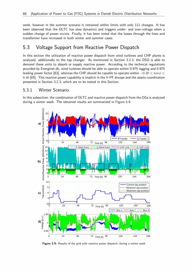
68 Application of Power to Gas (P2G) Systems in Danish Electric Distribution Networks
week, however in the summer scenario it remained within limits with only 111 changes. It hasbeen observed that the OLTC has slow dynamics and triggers under- and over-voltage when asudden change of power occurs. Finally, it has been noted that the losses through the lines andtransformer have increased in both winter and summer cases.
5.3 Voltage Support from Reactive Power DispatchIn this section the utilization of reactive power dispatch from wind turbines and CHP plants isanalyzed, additionally to the tap changer. As mentioned in Section 3.2.3, the DSO is able todemand these units to absorb or supply reactive power. According to the technical regulationsprovided by Energinet.dk, wind turbines should be able to operate within 0.975 lagging and 0.975leading power factor [63], whereas the CHP should be capable to operate within −0.20 ≤ tanφ ≤0.40 [65]. This reactive power capability is implicit in the V-PF droops and the assets coordinationpresented in Section 3.2.3, which are to be tested in this Section.
5.3.1 Winter ScenarioIn this subsection, the combination of OLTC and reactive power dispatch from the DGs is analyzedduring a winter week. The obtained results are summarized in Figure 5.9.
a)
b)
c)
d)
0 24 48 72 96 120 144 168
−5
0
5
10
Time [h]Act
ive/
Rea
ctiv
e P
ower
[MW
/MV
Ar]
−10 PP Feeder Q Feeder 1
0 24 48 72 96 120 144 168
−2
0
2
4
6
8
10
12
Time [h]
Act
ive/
Rea
ctiv
e P
ower
[MW
/MV
Ar]
P Wind Farm Q Wind Farm P CHP Unit Q CHP Unit
0 24 48 72 96 120 144 168
−5
0
5
10
Time [h]
Tap
pos
ition
]
−10
Current tap positionMinimum tap positionMaximum tap position
0 24 48 72 96 120 144 168
0.95
1
1.05
Time [h]
Vol
tage
[p.u
.]
Bus 1 Bus 7 Bus 9
Figure 5.9: Results of the grid with reactive power dispatch, during a winter week
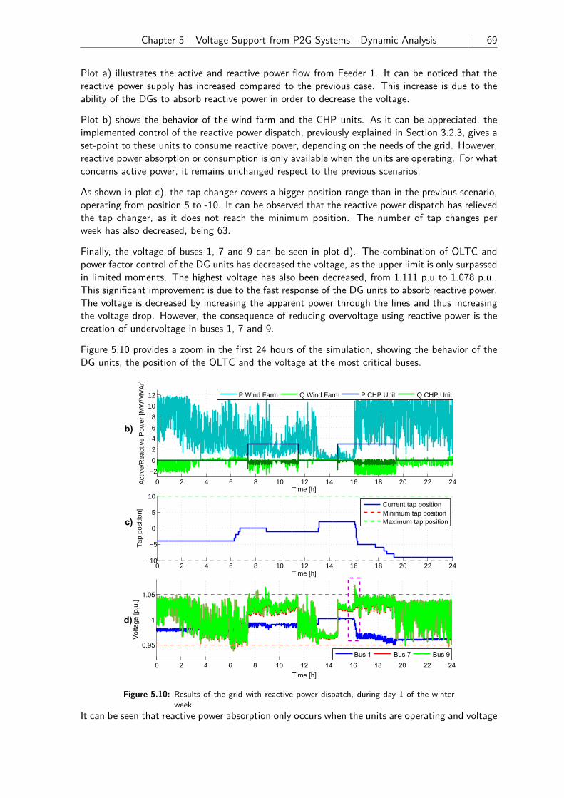
Chapter 5 - Voltage Support from P2G Systems - Dynamic Analysis 69
Plot a) illustrates the active and reactive power flow from Feeder 1. It can be noticed that thereactive power supply has increased compared to the previous case. This increase is due to theability of the DGs to absorb reactive power in order to decrease the voltage.
Plot b) shows the behavior of the wind farm and the CHP units. As it can be appreciated, theimplemented control of the reactive power dispatch, previously explained in Section 3.2.3, gives aset-point to these units to consume reactive power, depending on the needs of the grid. However,reactive power absorption or consumption is only available when the units are operating. For whatconcerns active power, it remains unchanged respect to the previous scenarios.
As shown in plot c), the tap changer covers a bigger position range than in the previous scenario,operating from position 5 to -10. It can be observed that the reactive power dispatch has relievedthe tap changer, as it does not reach the minimum position. The number of tap changes perweek has also decreased, being 63.
Finally, the voltage of buses 1, 7 and 9 can be seen in plot d). The combination of OLTC andpower factor control of the DG units has decreased the voltage, as the upper limit is only surpassedin limited moments. The highest voltage has also been decreased, from 1.111 p.u to 1.078 p.u..This significant improvement is due to the fast response of the DG units to absorb reactive power.The voltage is decreased by increasing the apparent power through the lines and thus increasingthe voltage drop. However, the consequence of reducing overvoltage using reactive power is thecreation of undervoltage in buses 1, 7 and 9.
Figure 5.10 provides a zoom in the first 24 hours of the simulation, showing the behavior of theDG units, the position of the OLTC and the voltage at the most critical buses.
b)
c)
d)
0 2 4 6 8 10 14 16 18 20 22 24
0.95
1
1.05
12Time [h]
Volta
ge [p
.u.]
Bus 1 Bus 7 Bus 9
0 2 4 6 8 10 12 14 16 18 20 22 24
−5
0
5
10
Time [h]
Tap
pos
ition
]
−10
Current tap positionMinimum tap positionMaximum tap position
0 2 4 6 8 10 12 14 16 18 20 22 24
−2
0
2
4
6
8
10
12
Time [h]
Act
ive/
Rea
ctiv
e P
ower
[MW
/MV
Ar]
P Wind Farm Q Wind Farm P CHP Unit Q CHP Unit
Figure 5.10: Results of the grid with reactive power dispatch, during day 1 of the winterweek
It can be seen that reactive power absorption only occurs when the units are operating and voltage
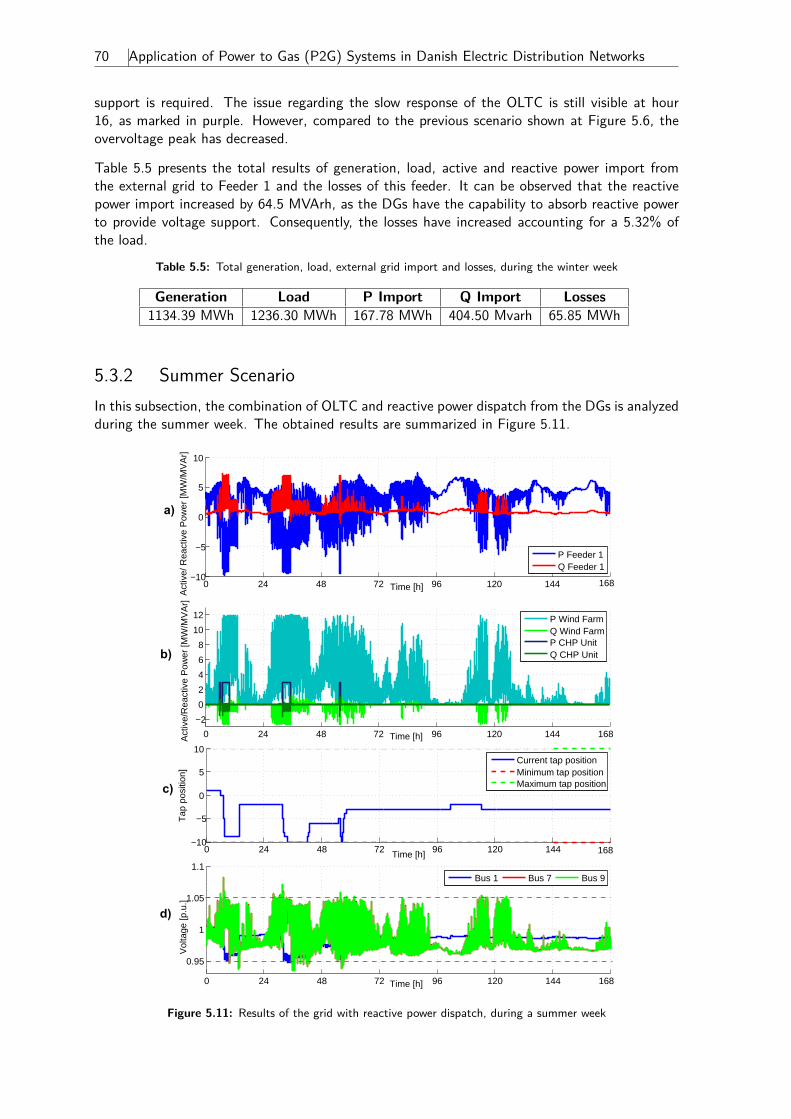
70 Application of Power to Gas (P2G) Systems in Danish Electric Distribution Networks
support is required. The issue regarding the slow response of the OLTC is still visible at hour16, as marked in purple. However, compared to the previous scenario shown at Figure 5.6, theovervoltage peak has decreased.
Table 5.5 presents the total results of generation, load, active and reactive power import fromthe external grid to Feeder 1 and the losses of this feeder. It can be observed that the reactivepower import increased by 64.5 MVArh, as the DGs have the capability to absorb reactive powerto provide voltage support. Consequently, the losses have increased accounting for a 5.32% ofthe load.
Table 5.5: Total generation, load, external grid import and losses, during the winter week
Generation Load P Import Q Import Losses1134.39 MWh 1236.30 MWh 167.78 MWh 404.50 Mvarh 65.85 MWh
5.3.2 Summer ScenarioIn this subsection, the combination of OLTC and reactive power dispatch from the DGs is analyzedduring the summer week. The obtained results are summarized in Figure 5.11.
a)
b)
c)
d)
0 24 48 72 96 120 144 168
−5
0
5
10
Time [h]
Act
ive/
Rea
ctiv
e P
ower
[MW
/MV
Ar]
−10
P Feeder 1Q Feeder 1
0 24 48 72 96 120 144 168
−2
0
2
4
6
8
10
12
Time [h]Act
ive/
Rea
ctiv
e P
ower
[MW
/MV
Ar]
P Wind FarmQ Wind FarmP CHP UnitQ CHP Unit
0 24 48 72 96 120 144 168
−5
0
5
10
Time [h]
Tap
pos
ition
]
−10
Current tap positionMinimum tap positionMaximum tap position
0 24 48 72 96 120 144 168
0.95
1
1.05
1.1
Time [h]
Vol
tage
[p.u
.]
Bus 1 Bus 7 Bus 9
Figure 5.11: Results of the grid with reactive power dispatch, during a summer week
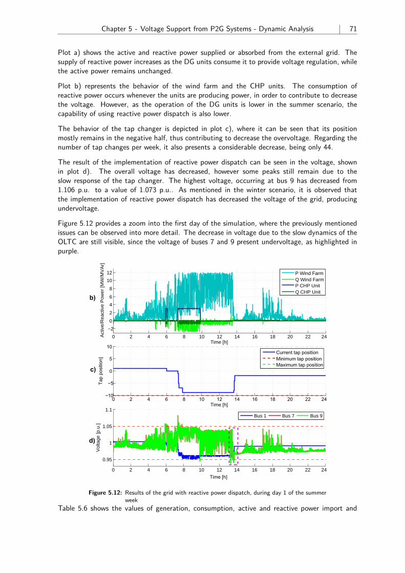
Chapter 5 - Voltage Support from P2G Systems - Dynamic Analysis 71
Plot a) shows the active and reactive power supplied or absorbed from the external grid. Thesupply of reactive power increases as the DG units consume it to provide voltage regulation, whilethe active power remains unchanged.
Plot b) represents the behavior of the wind farm and the CHP units. The consumption ofreactive power occurs whenever the units are producing power, in order to contribute to decreasethe voltage. However, as the operation of the DG units is lower in the summer scenario, thecapability of using reactive power dispatch is also lower.
The behavior of the tap changer is depicted in plot c), where it can be seen that its positionmostly remains in the negative half, thus contributing to decrease the overvoltage. Regarding thenumber of tap changes per week, it also presents a considerable decrease, being only 44.
The result of the implementation of reactive power dispatch can be seen in the voltage, shownin plot d). The overall voltage has decreased, however some peaks still remain due to theslow response of the tap changer. The highest voltage, occurring at bus 9 has decreased from1.106 p.u. to a value of 1.073 p.u.. As mentioned in the winter scenario, it is observed thatthe implementation of reactive power dispatch has decreased the voltage of the grid, producingundervoltage.
Figure 5.12 provides a zoom into the first day of the simulation, where the previously mentionedissues can be observed into more detail. The decrease in voltage due to the slow dynamics of theOLTC are still visible, since the voltage of buses 7 and 9 present undervoltage, as highlighted inpurple.
b)
c)
d)
0 2 4 6 8 10 12 14 16 18 20 22 24
0.95
1
1.05
1.1
Vol
tage
[p.u
.]
Bus 1 Bus 7 Bus 9
0 2 4 6 8 10 12 14 16 18 20 22 24
−5
0
5
10
Time [h]
Tap
posi
tion]
−10
Current tap positionMinimum tap positionMaximum tap position
Time [h]
0 2 4 6 8 10 12 14 16 18 20 22 24
−2
0
2
4
6
8
10
12
Time [h]
Act
ive/
Rea
ctiv
e P
ower
[MW
/MV
Ar]
P Wind FarmQ Wind FarmP CHP UnitQ CHP Unit
Figure 5.12: Results of the grid with reactive power dispatch, during day 1 of the summerweek
Table 5.6 shows the values of generation, consumption, active and reactive power import and
72 Application of Power to Gas (P2G) Systems in Danish Electric Distribution Networks
grid losses at the end of the week. In this case, the import of reactive power does not present abig increase as in the winter case. This is due to the reduced time of operation of the DG unitscompared to the winter case. The losses account for a 2.62% of the load, a higher value than inthe previous scenario.
Table 5.6: Total generation, load, external grid import and losses, during the summer week
Generation Load P Import Q Import Losses426.15 MWh 712.80 MWh 305.44 MWh 178.70 Mvarh 18.66 MWh
5.3.3 SummaryIn this section, the integration of reactive power compensation together with the OLTC has beenanalyzed. As seen in both winter and summer scenarios, the overvoltage issue presented in Section5.2 has been improved. Overvoltage is now limited to extreme cases of sudden power increase,partly due to the issue presented by the slow dynamics of the OLTC. On the other hand, theimplementation of reactive power compensation is not ideal as it creates undervoltage in bus 1.As specified in Figure 5.12, the OLTC decreased the voltage to nearly 0.95 p.u. by changing itsposition, and the reactive power flow aggravates it further. Therefore, it should only be utilizedin extreme conditions
As summarized in Tables 5.5 and 5.6, the reactive power import to the grid increased, as the CHPunits and wind turbines utilize reactive power to create a voltage decrease. Consequently, thelosses increased, with values of 5.32% and 2.62% of the total consumption in winter and summercases respectively.
5.4 Voltage Support from Alkaline ElectrolyzersAs it has been previously analyzed in sections 5.2 and 5.3, the implementation of an OLTCand reactive power dispatch from wind turbines and CHP units is not enough to correct theovervoltage that the grid presented initially, as explained in Section 5.1. Therefore, the aim ofthis scenario is to evaluate the efficacy of implementing a Power to Gas System in order to providevoltage regulation to the studied distribution grid. A first steady state analysis was carried out inSection 3.2.4, where its location was determined to be in bus 9, and have a size of 6.525 MW.Furthermore, the coordination of the the OLTC, DGs’ reactive power and alkaline electrolyzer,presented in the mentioned Section, is now tested.
As done in the previous scenarios, the presented results for the winter and summer cases includethe active and reactive power flow from Feeder 1, the production of the DG, operation of OLTCand the voltage profile during the week. Additionally, the basic parameters of the electrolyzerunits are presented, such as active and reactive power consumption, operating temperature andhydrogen production.
5.4.1 Winter ScenarioFigure 5.13 illustrates the results of the implementation of P2G in the distribution grid duringwinter scenario. It can be seen in plot a) that the power exported to the external grid is consid-erably lower, as part of the locally produced power is now utilized by the electrolyzer units. Thisresult demonstrates the capability of the installed electrolyzers to provide energy managementand, at the same time provide voltage support.
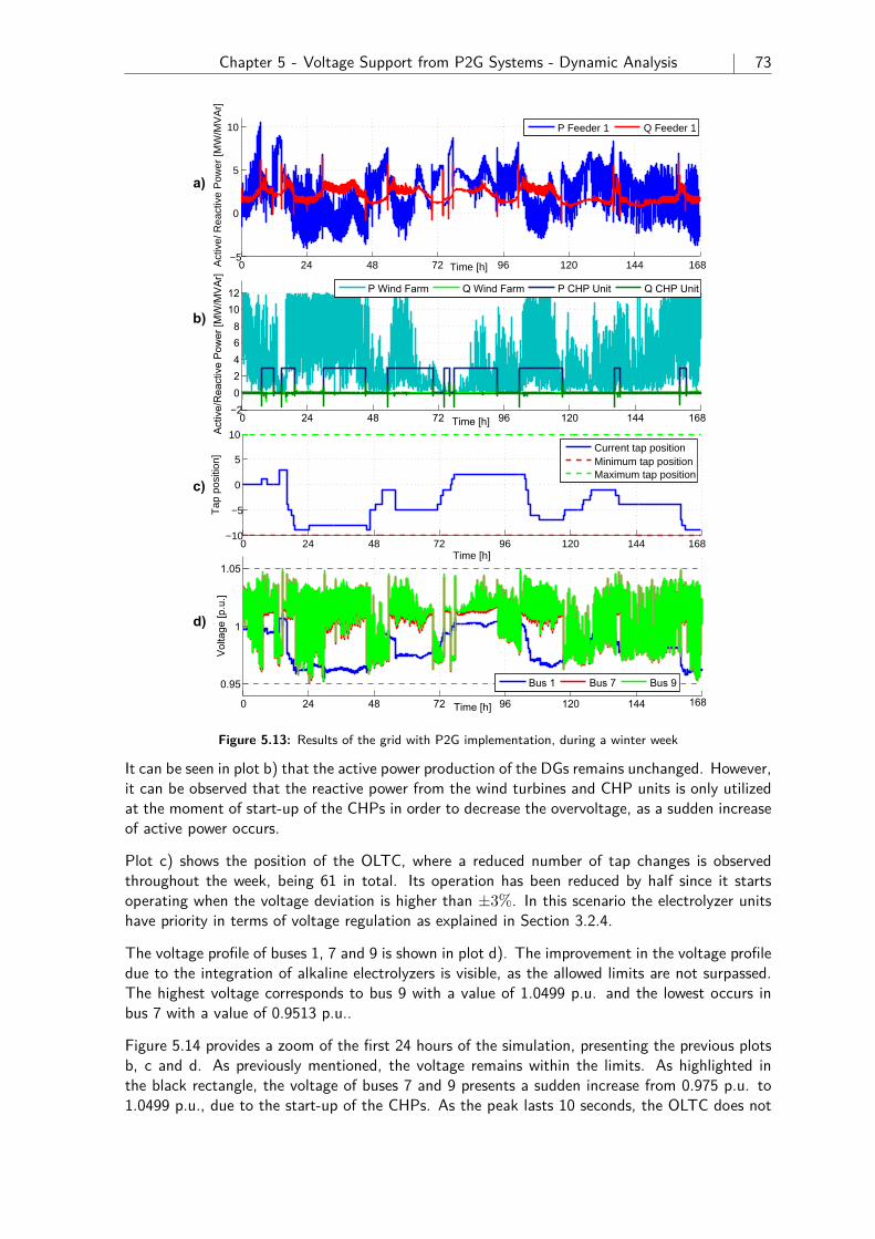
Chapter 5 - Voltage Support from P2G Systems - Dynamic Analysis 73
0 24 48 72 96 120 144 168
0.95
1
1.05
Time [h]
Volta
ge [p
.u.]
Bus 1 Bus 7 Bus 9
a)
c)
b)
d)
0 24 48 72 96 120 144 168
−5
0
5
10
Time [h]
Tap
pos
ition
]
−10
Current tap positionMinimum tap positionMaximum tap position
0 24 48 72 96 120 144 168
02468
1012
Time [h]
Activ
e/R
eact
ive
Pow
er [M
W/M
VAr]
−2
P Wind Farm Q Wind Farm P CHP Unit Q CHP Unit
0 24 48 72 96 120 144 168
0
5
10
Time [h]Act
ive/
Rea
ctiv
e P
ower
[MW
/MV
Ar]
−5
P Feeder 1 Q Feeder 1
Figure 5.13: Results of the grid with P2G implementation, during a winter week
It can be seen in plot b) that the active power production of the DGs remains unchanged. However,it can be observed that the reactive power from the wind turbines and CHP units is only utilizedat the moment of start-up of the CHPs in order to decrease the overvoltage, as a sudden increaseof active power occurs.
Plot c) shows the position of the OLTC, where a reduced number of tap changes is observedthroughout the week, being 61 in total. Its operation has been reduced by half since it startsoperating when the voltage deviation is higher than ±3%. In this scenario the electrolyzer unitshave priority in terms of voltage regulation as explained in Section 3.2.4.
The voltage profile of buses 1, 7 and 9 is shown in plot d). The improvement in the voltage profiledue to the integration of alkaline electrolyzers is visible, as the allowed limits are not surpassed.The highest voltage corresponds to bus 9 with a value of 1.0499 p.u. and the lowest occurs inbus 7 with a value of 0.9513 p.u..
Figure 5.14 provides a zoom of the first 24 hours of the simulation, presenting the previous plotsb, c and d. As previously mentioned, the voltage remains within the limits. As highlighted inthe black rectangle, the voltage of buses 7 and 9 presents a sudden increase from 0.975 p.u. to1.0499 p.u., due to the start-up of the CHPs. As the peak lasts 10 seconds, the OLTC does not
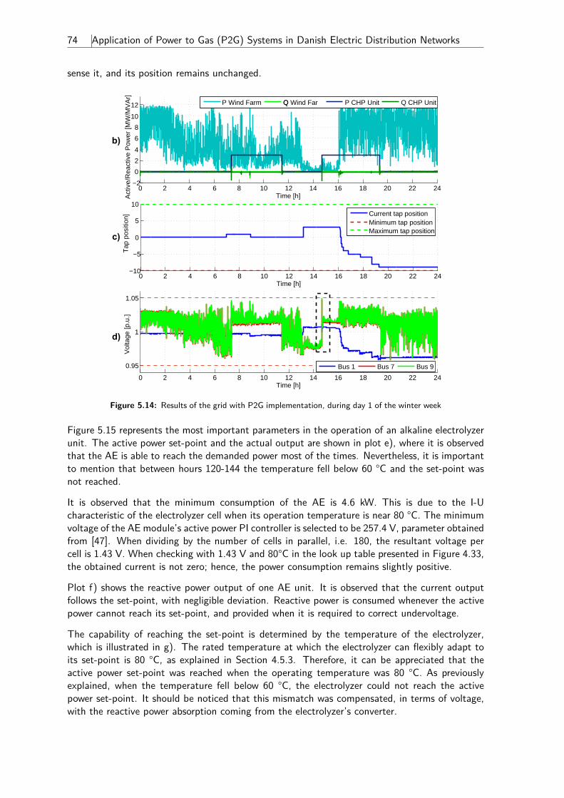
74 Application of Power to Gas (P2G) Systems in Danish Electric Distribution Networks
sense it, and its position remains unchanged.
0 2 4 6 8 10 12 14 16 18 20 22 24
0.95
1
1.05
Time [h]
Vol
tage
[p.u
.]
Bus 1 Bus 7 Bus 9
0 2 4 6 8 10 12 14 16 18 20 22 24
−5
0
5
10
Time [h]
Tap
pos
ition
]
−10
Current tap positionMinimum tap positionMaximum tap position
0 2 4 6 8 10 12 14 16 18 20 22 24
0
2
4
6
8
10
12
Time [h]Act
ive/
Rea
ctiv
e P
ower
[MW
/MV
Ar]
−2
P Wind Farm QQ Wind Far P CHP Unit Q CHP Unit
c)
b)
d)
Figure 5.14: Results of the grid with P2G implementation, during day 1 of the winter week
Figure 5.15 represents the most important parameters in the operation of an alkaline electrolyzerunit. The active power set-point and the actual output are shown in plot e), where it is observedthat the AE is able to reach the demanded power most of the times. Nevertheless, it is importantto mention that between hours 120-144 the temperature fell below 60 °C and the set-point wasnot reached.
It is observed that the minimum consumption of the AE is 4.6 kW. This is due to the I-Ucharacteristic of the electrolyzer cell when its operation temperature is near 80 °C. The minimumvoltage of the AE module’s active power PI controller is selected to be 257.4 V, parameter obtainedfrom [47]. When dividing by the number of cells in parallel, i.e. 180, the resultant voltage percell is 1.43 V. When checking with 1.43 V and 80°C in the look up table presented in Figure 4.33,the obtained current is not zero; hence, the power consumption remains slightly positive.
Plot f) shows the reactive power output of one AE unit. It is observed that the current outputfollows the set-point, with negligible deviation. Reactive power is consumed whenever the activepower cannot reach its set-point, and provided when it is required to correct undervoltage.
The capability of reaching the set-point is determined by the temperature of the electrolyzer,which is illustrated in g). The rated temperature at which the electrolyzer can flexibly adapt toits set-point is 80 °C, as explained in Section 4.5.3. Therefore, it can be appreciated that theactive power set-point was reached when the operating temperature was 80 °C. As previouslyexplained, when the temperature fell below 60 °C, the electrolyzer could not reach the activepower set-point. It should be noticed that this mismatch was compensated, in terms of voltage,with the reactive power absorption coming from the electrolyzer’s converter.
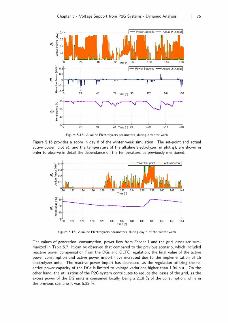
Chapter 5 - Voltage Support from P2G Systems - Dynamic Analysis 75
0 24 48 72 96 120 144 16820
40
60
80
Time [h]
Tem
pera
ture
[ºC
]
0 24 48 72 96 120 144 168
−0.1
0
0.1
0.2
Time [h]
Rea
ctiv
e P
ower
[MV
Ar]
−0.2
Power Setpoint Actual Q Output
0 24 48 72 96 120 144 168
0.1
0.2
0.3
0.4
Time [h]
Act
ive
Pow
er [M
W]
0
Power Setpoint Actual P Output
e)
g)
f)
Figure 5.15: Alkaline Electrolyzers parameters, during a winter week
Figure 5.16 provides a zoom in day 6 of the winter week simulation. The set-point and actualactive power, plot e), and the temperature of the alkaline electrolyzer, in plot g), are shown inorder to observe in detail the dependance on the temperature, as previously mentioned.
120 122 124 126 128 130 132 134 136 138 140 142 1440
0.1
0.2
0.3
0.4
Time [h]
Act
ive
Pow
er [M
W]
Power Set-point Actual Output
120 122 124 126 128 130 132 134 136 138 140 142 14420
40
60
80
Time [h]
Tem
pera
ture
[ºC
]
e)
g)
Figure 5.16: Alkaline Electrolyzers parameters, during day 5 of the winter week
The values of generation, consumption, power flow from Feeder 1 and the grid losses are sum-marized in Table 5.7. It can be observed that compared to the previous scenario, which includedreactive power compensation from the DGs and OLTC regulation, the final value of the activepower consumption and active power import have increased due to the implementation of 15electrolyzer units. The reactive power import has decreased, as the regulation utilizing the re-active power capacity of the DGs is limited to voltage variations higher than 1.04 p.u.. On theother hand, the utilization of the P2G system contributes to reduce the losses of the grid, as theexcess power of the DG units is consumed locally, being a 2.18 % of the consumption, while inthe previous scenario it was 5.32 %.
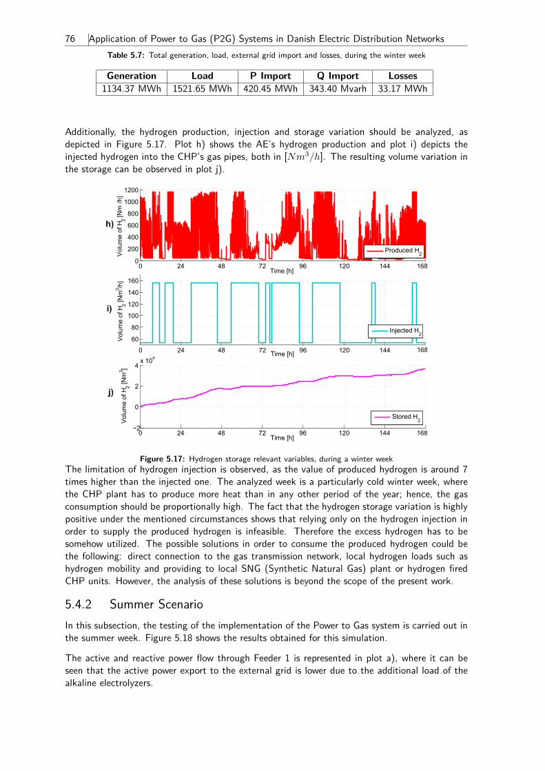
76 Application of Power to Gas (P2G) Systems in Danish Electric Distribution NetworksTable 5.7: Total generation, load, external grid import and losses, during the winter week
Generation Load P Import Q Import Losses1134.37 MWh 1521.65 MWh 420.45 MWh 343.40 Mvarh 33.17 MWh
Additionally, the hydrogen production, injection and storage variation should be analyzed, asdepicted in Figure 5.17. Plot h) shows the AE’s hydrogen production and plot i) depicts theinjected hydrogen into the CHP’s gas pipes, both in [Nm3/h]. The resulting volume variation inthe storage can be observed in plot j).
0 24 48 72 96 120 144 1680
200
400
600
800
1000
1200
Time [h]
Volu
me
of H
2 [Nm
/h]
0 24 48 72 96 120 144 168−2
0
2
4x 10⁴
Time [h]
Volu
me
of H
2 [Nm
3 ]
0 24 48 72 96 120 144 16860
80
100
120
140
160
Time [h]
Volu
me
of H
2 [Nm
3 /h]
h)
i)
j)
Produced H2
Injected H2
Stored H2
Figure 5.17: Hydrogen storage relevant variables, during a winter weekThe limitation of hydrogen injection is observed, as the value of produced hydrogen is around 7times higher than the injected one. The analyzed week is a particularly cold winter week, wherethe CHP plant has to produce more heat than in any other period of the year; hence, the gasconsumption should be proportionally high. The fact that the hydrogen storage variation is highlypositive under the mentioned circumstances shows that relying only on the hydrogen injection inorder to supply the produced hydrogen is infeasible. Therefore the excess hydrogen has to besomehow utilized. The possible solutions in order to consume the produced hydrogen could bethe following: direct connection to the gas transmission network, local hydrogen loads such ashydrogen mobility and providing to local SNG (Synthetic Natural Gas) plant or hydrogen firedCHP units. However, the analysis of these solutions is beyond the scope of the present work.
5.4.2 Summer ScenarioIn this subsection, the testing of the implementation of the Power to Gas system is carried out inthe summer week. Figure 5.18 shows the results obtained for this simulation.
The active and reactive power flow through Feeder 1 is represented in plot a), where it can beseen that the active power export to the external grid is lower due to the additional load of thealkaline electrolyzers.
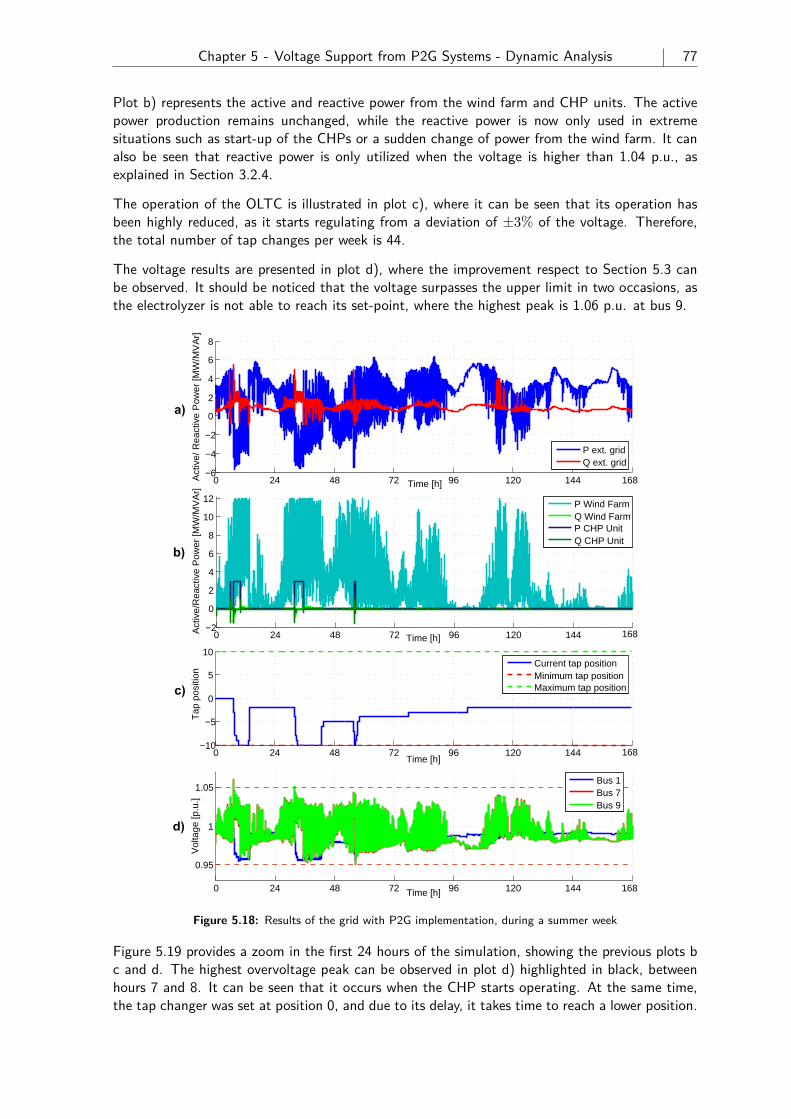
Chapter 5 - Voltage Support from P2G Systems - Dynamic Analysis 77
Plot b) represents the active and reactive power from the wind farm and CHP units. The activepower production remains unchanged, while the reactive power is now only used in extremesituations such as start-up of the CHPs or a sudden change of power from the wind farm. It canalso be seen that reactive power is only utilized when the voltage is higher than 1.04 p.u., asexplained in Section 3.2.4.
The operation of the OLTC is illustrated in plot c), where it can be seen that its operation hasbeen highly reduced, as it starts regulating from a deviation of ±3% of the voltage. Therefore,the total number of tap changes per week is 44.
The voltage results are presented in plot d), where the improvement respect to Section 5.3 canbe observed. It should be noticed that the voltage surpasses the upper limit in two occasions, asthe electrolyzer is not able to reach its set-point, where the highest peak is 1.06 p.u. at bus 9.
0 24 48 72 96 120 144 168
0.95
1
1.05
Time [h]
Vol
tage
[p.u
.]
Bus 1Bus 7Bus 9
0 24 48 72 96 120 144 168
−5
0
5
10
Time [h]
Tap
pos
ition
−10
Current tap positionMinimum tap positionMaximum tap position
0 24 48 72 96 120 144 168
0
2
4
6
8
10
12
Time [h]
Act
ive/
Rea
ctiv
e P
ower
[MW
/MV
Ar]
−2
P Wind FarmQ Wind FarmP CHP UnitQ CHP Unit
0 24 48 72 96 120 144 168
−4
−2
0
2
4
6
8
Time [h]
Act
ive/
Rea
ctiv
e P
ower
[MW
/MV
Ar]
−6
P ext. gridQ ext. grid
a)
c)
b)
d)
Figure 5.18: Results of the grid with P2G implementation, during a summer week
Figure 5.19 provides a zoom in the first 24 hours of the simulation, showing the previous plots bc and d. The highest overvoltage peak can be observed in plot d) highlighted in black, betweenhours 7 and 8. It can be seen that it occurs when the CHP starts operating. At the same time,the tap changer was set at position 0, and due to its delay, it takes time to reach a lower position.
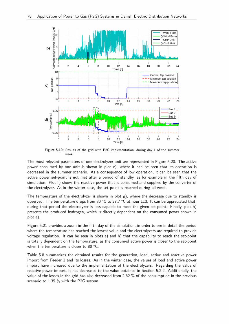
78 Application of Power to Gas (P2G) Systems in Danish Electric Distribution Networks
0 2 4 6 8 10 12 14 16 18 20 22 24
0
5
10
Time [h]Act
ive/
Rea
ctiv
e P
ower
[MW
/MV
Ar]
P Wind FarmQ Wind FarmP CHP UnitQ CHP Unit
0 2 4 6 8 10 12 14 16 18 20 22 24
−5
0
5
10
Time [h]
Tap
pos
ition
−10
Current tap positionMinimum tap positionMaximum tap position
b)
c)
d)
0 2 4 6 8 10 12 14 16 18 20 22 24
0.95
1
1.05
Time [h]
Vol
tage
[p.u
.]
Bus 1Bus 7Bus 9
Figure 5.19: Results of the grid with P2G implementation, during day 1 of the summerweek
The most relevant parameters of one electrolyzer unit are represented in Figure 5.20. The activepower consumed by one unit is shown in plot e), where it can be seen that its operation isdecreased in the summer scenario. As a consequence of low operation, it can be seen that theactive power set-point is not met after a period of standby, as for example in the fifth day ofsimulation. Plot f) shows the reactive power that is consumed and supplied by the converter ofthe electrolyzer. As in the winter case, the set-point is reached during all week.
The temperature of the electrolyzer is shown in plot g), where the decrease due to standby isobserved. The temperature drops from 80 °C to 27.7 °C at hour 113. It can be appreciated that,during that period the electrolyzer is less capable to meet the given set-point. Finally, plot h)presents the produced hydrogen, which is directly dependent on the consumed power shown inplot e).
Figure 5.21 provides a zoom in the fifth day of the simulation, in order to see in detail the periodwhere the temperature has reached the lowest value and the electrolyzers are required to providevoltage regulation. It can be seen in plots e) and h) that the capability to reach the set-pointis totally dependent on the temperature, as the consumed active power is closer to the set-pointwhen the temperature is closer to 80 °C.
Table 5.8 summarizes the obtained results for the generation, load, active and reactive powerimport from Feeder 1 and its losses. As in the winter case, the values of load and active powerimport have increased due to the implementation of the electrolyzers. Regarding the value ofreactive power import, it has decreased to the value obtained in Section 5.2.2. Additionally, thevalue of the losses in the grid has also decreased from 2.62 % of the consumption in the previousscenario to 1.35 % with the P2G system.
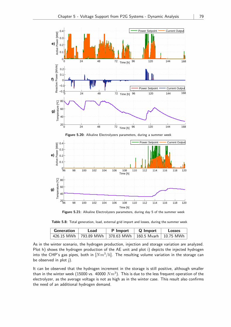
Chapter 5 - Voltage Support from P2G Systems - Dynamic Analysis 79
0 24 48 72 96 120 144 16820
40
60
80
Time [h]
Tem
pera
ture
[ºC
]
0 24 48 72 96 120 144 168
−0.1
0
0.1
0.2
Time [h]
Rea
ctiv
e P
ower
[MV
Ar]
−0.2 Power Setpoint Current Output
0 24 48 72 96 120 144 168
0.1
0.2
0.3
0.4
Time [h]
Act
ive
Pow
er [M
W]
0
Power Setpoint Current Output
e)
g)
f)
Figure 5.20: Alkaline Electrolyzers parameters, during a summer week
96 98 100 102 104 106 108 110 112 114 116 118 12020
40
60
80
Time [h]
Tem
pera
ture
[ºC
]
96 98 100 102 104 106 108 110 112 114 116 118 120
0.1
0.2
0.3
0.4
Time [h]
Act
ive
Pow
er [M
W]
0
Power Setpoint Current Output
e)
g)
As in the winter scenario, the hydrogen production, injection and storage variation are analyzed.Plot h) shows the hydrogen production of the AE unit and plot i) depicts the injected hydrogeninto the CHP’s gas pipes, both in [Nm3/h]. The resulting volume variation in the storage canbe observed in plot j).
It can be observed that the hydrogen increment in the storage is still positive, although smallerthan in the winter week (15000 vs. 40000 Nm3). This is due to the less frequent operation of theelectrolyzer, as the average voltage is not as high as in the winter case. This result also confirmsthe need of an additional hydrogen demand.
Table 5.8: Total generation, load, external grid import and losses, during the summer week
Generation Load P Import Q Import Losses426.15 MWh 793.89 MWh 378.63 MWh 160.5 Mvarh 10.75 MWh
Figure 5.21: Alkaline Electrolyzers parameters, during day 5 of the summer week
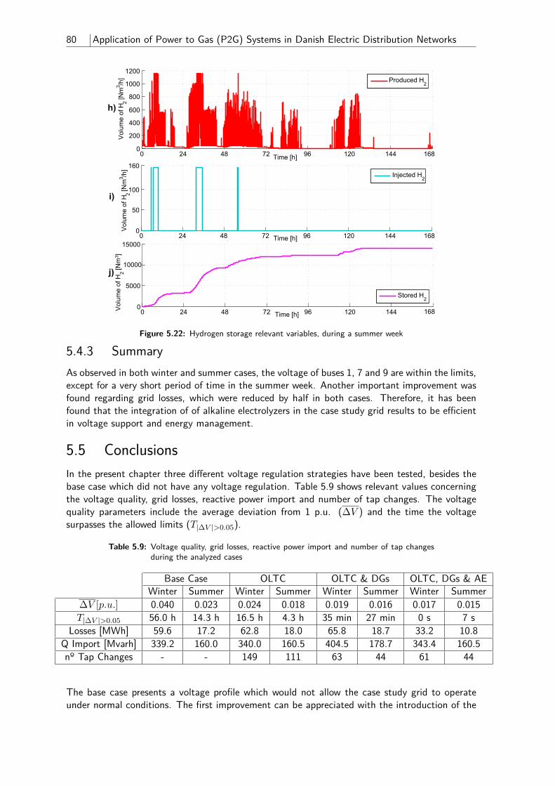
80 Application of Power to Gas (P2G) Systems in Danish Electric Distribution Networks
0 24 48 72 96 120 144 1680
200
400
600
800
1000
1200
Time [h]
Volu
me
of H
2 [Nm
3 /h]
0 24 48 72 96 120 144 1680
50
100
160
Time [h]
Volu
me
of H
2 [Nm
3 /h]
0 24 48 72 96 120 144 1680
5000
10000
15000
Time [h]
Volu
me
of H
2 [Nm
3 ]h)
i)
j)
Produced H2
Injected H2
Stored H2
Figure 5.22: Hydrogen storage relevant variables, during a summer week
5.4.3 SummaryAs observed in both winter and summer cases, the voltage of buses 1, 7 and 9 are within the limits,except for a very short period of time in the summer week. Another important improvement wasfound regarding grid losses, which were reduced by half in both cases. Therefore, it has beenfound that the integration of of alkaline electrolyzers in the case study grid results to be efficientin voltage support and energy management.
5.5 ConclusionsIn the present chapter three different voltage regulation strategies have been tested, besides thebase case which did not have any voltage regulation. Table 5.9 shows relevant values concerningthe voltage quality, grid losses, reactive power import and number of tap changes. The voltagequality parameters include the average deviation from 1 p.u. (∆V ) and the time the voltagesurpasses the allowed limits (T|∆V |>0.05).
Table 5.9: Voltage quality, grid losses, reactive power import and number of tap changesduring the analyzed cases
Base Case OLTC OLTC & DGs OLTC, DGs & AEWinter Summer Winter Summer Winter Summer Winter Summer
∆V [p.u.] 0.040 0.023 0.024 0.018 0.019 0.016 0.017 0.015T|∆V |>0.05 56.0 h 14.3 h 16.5 h 4.3 h 35 min 27 min 0 s 7 s
Losses [MWh] 59.6 17.2 62.8 18.0 65.8 18.7 33.2 10.8Q Import [Mvarh] 339.2 160.0 340.0 160.5 404.5 178.7 343.4 160.5nº Tap Changes - - 149 111 63 44 61 44
The base case presents a voltage profile which would not allow the case study grid to operateunder normal conditions. The first improvement can be appreciated with the introduction of the
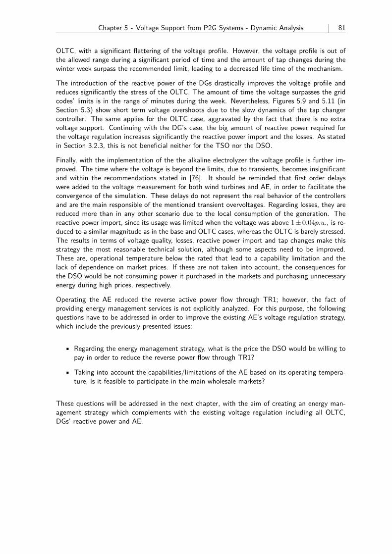
Chapter 5 - Voltage Support from P2G Systems - Dynamic Analysis 81
OLTC, with a significant flattering of the voltage profile. However, the voltage profile is out ofthe allowed range during a significant period of time and the amount of tap changes during thewinter week surpass the recommended limit, leading to a decreased life time of the mechanism.
The introduction of the reactive power of the DGs drastically improves the voltage profile andreduces significantly the stress of the OLTC. The amount of time the voltage surpasses the gridcodes’ limits is in the range of minutes during the week. Nevertheless, Figures 5.9 and 5.11 (inSection 5.3) show short term voltage overshoots due to the slow dynamics of the tap changercontroller. The same applies for the OLTC case, aggravated by the fact that there is no extravoltage support. Continuing with the DG’s case, the big amount of reactive power required forthe voltage regulation increases significantly the reactive power import and the losses. As statedin Section 3.2.3, this is not beneficial neither for the TSO nor the DSO.
Finally, with the implementation of the the alkaline electrolyzer the voltage profile is further im-proved. The time where the voltage is beyond the limits, due to transients, becomes insignificantand within the recommendations stated in [76]. It should be reminded that first order delayswere added to the voltage measurement for both wind turbines and AE, in order to facilitate theconvergence of the simulation. These delays do not represent the real behavior of the controllersand are the main responsible of the mentioned transient overvoltages. Regarding losses, they arereduced more than in any other scenario due to the local consumption of the generation. Thereactive power import, since its usage was limited when the voltage was above 1±0.04p.u., is re-duced to a similar magnitude as in the base and OLTC cases, whereas the OLTC is barely stressed.The results in terms of voltage quality, losses, reactive power import and tap changes make thisstrategy the most reasonable technical solution, although some aspects need to be improved.These are, operational temperature below the rated that lead to a capability limitation and thelack of dependence on market prices. If these are not taken into account, the consequences forthe DSO would be not consuming power it purchased in the markets and purchasing unnecessaryenergy during high prices, respectively.
Operating the AE reduced the reverse active power flow through TR1; however, the fact ofproviding energy management services is not explicitly analyzed. For this purpose, the followingquestions have to be addressed in order to improve the existing AE’s voltage regulation strategy,which include the previously presented issues:
• Regarding the energy management strategy, what is the price the DSO would be willing topay in order to reduce the reverse power flow through TR1?
• Taking into account the capabilities/limitations of the AE based on its operating tempera-ture, is it feasible to participate in the main wholesale markets?
These questions will be addressed in the next chapter, with the aim of creating an energy man-agement strategy which complements with the existing voltage regulation including all OLTC,DGs’ reactive power and AE.

Chapter 6 - Energy Management from P2G Systems - Market and Dynamic Analysis 83
6 Energy Management from P2G Systems- Market Strategy and Dynamic Analysis
In this chapter an improvement of the voltage regulation strategy provided in Section 5.4 ispresented. As stated in Chapter 5, the active power absorbed by the electrolyzer did not take intoconsideration the electricity market prices. Moreover, providing energy management services, i.e.minimizing the active power export through TR1, was not explicitly analyzed. Therefore, the aimof this chapter is to develop a market strategy that copes with both the voltage regulation andenergy management requirements. Nevertheless, the market strategy will need to deal with twodifferent issues:
• The capability of the AE is limited by its operation temperature, which might bring eco-nomical consequences when participating in the electricity markets
• Energy management and voltage regulation are services which have a benefit for the DSO,although the associated economical benefit of these services cannot be easily established inthis specific work
Regarding the dynamic analysis, the AE control models depicted in Figure 4.28 and Figure 4.29,in Section 4.5, will be modified in order to incorporate the active power set-points of the presentedstrategy. Additionally, a new coordination of the OLTC, reactive power of the DG and active andreactive power of the AE will be presented in order to keep a balance among different constraints:
• Maintaining the voltage within the allowed limits, as in the results obtained in Section 5.4
• Daily number of tap changes below 20
• Reduce as much as possible the active power deviations from the schedule
• Keep the reactive power import as low as possible
In the following section, the market strategy is explained and the steady state hourly results arepresented, both technical and economical. Furthermore, the economical results are compared tothe average values obtained in Section 5.4, in order to determine the achieved improvement.
6.1 Market Strategy - Steady State Analysis6.1.1 IntroductionThe purpose of this section is to provide an overview of the developed market strategy. Firstly,the approach taken in the strategy is explained, where the different markets, the market playersand the process to determine the schedule of the AE, are introduced. Secondly, a detailed schemeof the strategy is presented, where the differentiated parts in which the bid is calculated, areexplained. This explanation includes the data exchange between the differentiated parts and theflowchart with the logical sequence of the market strategy.
84 Application of Power to Gas (P2G) Systems in Danish Electric Distribution Networks
Approach: markets, players and scheduling process
The target of the implemented market strategy is to schedule the hourly operation of the AEaccording to the technical requirements of the grid and the market prices. For this purpose, thedifferent markets in which the AE takes part and the different players involved in the biddingprocess are introduced. In the following, the most important characteristics of the analyzedmarkets are presented, in order to know the different time windows in which the bids have tobe made. The analyzed markets are: the spot market (Elspot), the intraday market (Elbas) andthe regulation power market. The presented information has been taken from Appendix A, wheremore detailed information about the electricity markets can be found. As explained in Section2.3, a new market for flexibility is still to be introduced, where the grid companies can avoidcongestion by participating in it. Therefore, the implemented strategy only takes into accountthe currently existing markets.
• Elspot: This market closes at 12:00 am the day before delivery and bids are made for a 24hour period corresponding to a natural day.
• Elbas: Bids can be forwarded from the closing of the Elspot market until 1h prior operation.The bidding period is assumed to be one hour. When deciding the volume of the bid, thealready purchased power in the spot market has to be taken into account.
• Regulation Power Market: Bids have to be forwarded before 17:00 the day prior operation;nevertheless, they can be modified up to 1 hour before. The minimum size of the bids is10 MW and the bidding period is 1 hour. The regulation power has the peculiarity that itis activated only when the TSO requires it. Furthermore, activation time should not takelonger than 15 minutes. It should be noticed that the electrolyzer might not be able tofulfill this condition if its temperature is not high enough. Since the AE is a load, only downregulation is considered.
In the following, the market players, i.e. DSOs and BRPs, are presented.
• DSOs: Normally they do not participate in the electricity markets. However, as study gridDSO requires active power for the electrolyzer, it will purchase electricity directly in thewholesale markets. For this purpose, it has to have an agreement with a BRP in orderto balance the schedule. In this context, the DSO forwards the bid to the BRP, who isresponsible for placing the bid in the market. As stated in Section 2.2, DSOs are expectedto be customers of the upcoming flexibility market. However, this flexibility market is notcompletely developed nowadays and DSOs have to obtain the flexibility by scheduling theelectrolyzer in an intelligent way. In other words, instead of aggregators and BRPs offeringproducts to the DSOs in the flexibility market, these have to create the flexibility on theirown.
• BRPs: They possess agreements with different producers, traders and big consumers, whichincludes the DSOs. They receive the bid forwarded by the DSO, aggregates it with the bidsforwarded by the rest of the BRP’s customers and places the aggregated bid in the market.This is relevant when analyzing the participation of the DSOs in the regulating power marketas the rated power of the AE is 6.525 MW but the minimum bid is 10 MW. Thus, it isassumed that the BRP possesses more regulation capacity that allows the bid to reach 10MW.
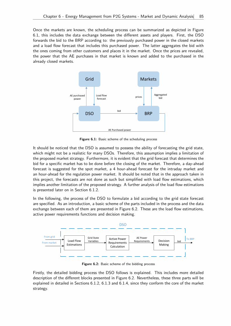
Chapter 6 - Energy Management from P2G Systems - Market and Dynamic Analysis 85
Once the markets are known, the scheduling process can be summarized as depicted in Figure6.1, this includes the data exchange between the different assets and players. First, the DSOforwards the bid to the BRP according to: the previously purchased power in the closed marketsand a load flow forecast that includes this purchased power. The latter aggregates the bid withthe ones coming from other customers and places it in the market. Once the prices are revealed,the power that the AE purchases in that market is known and added to the purchased in thealready closed markets.
DSO BRP
Grid Markets
bid
AE Purchased power
Aggregated bidprices
Load flow forecast
AE purchased power
Figure 6.1: Basic scheme of the scheduling process
It should be noticed that the DSO is assumed to possess the ability of forecasting the grid state,which might not be a realistic for many DSOs. Therefore, this assumption implies a limitation ofthe proposed market strategy. Furthermore, it is evident that the grid forecast that determines thebid for a specific market has to be done before the closing of the market. Therefore, a day-aheadforecast is suggested for the spot market, a 4 hour-ahead forecast for the intraday market andan hour-ahead for the regulation power market. It should be noted that in the approach taken inthis project, the forecasts are not done as such but simplified with load flow estimations, whichimplies another limitation of the proposed strategy. A further analysis of the load flow estimationsis presented later on in Section 6.1.2.
In the following, the process of the DSO to formulate a bid according to the grid state forecastare specified. As an introduction, a basic scheme of the parts included in the process and the dataexchange between each of them are presented in Figure 6.2. These are the load flow estimations,active power requirements functions and decision making.
Load Flow Estimations
Active Power Requirements Calculation
Decision Making
Grid State Variables
AE Power Requirements bid
DSO
From grid
From market
To BRP
Figure 6.2: Basic scheme of the bidding process
Firstly, the detailed bidding process the DSO follows is explained. This includes more detaileddescription of the different blocks presented in Figure 6.2. Nevertheless, these three parts will beexplained in detailed in Sections 6.1.2, 6.1.3 and 6.1.4, since they conform the core of the marketstrategy.
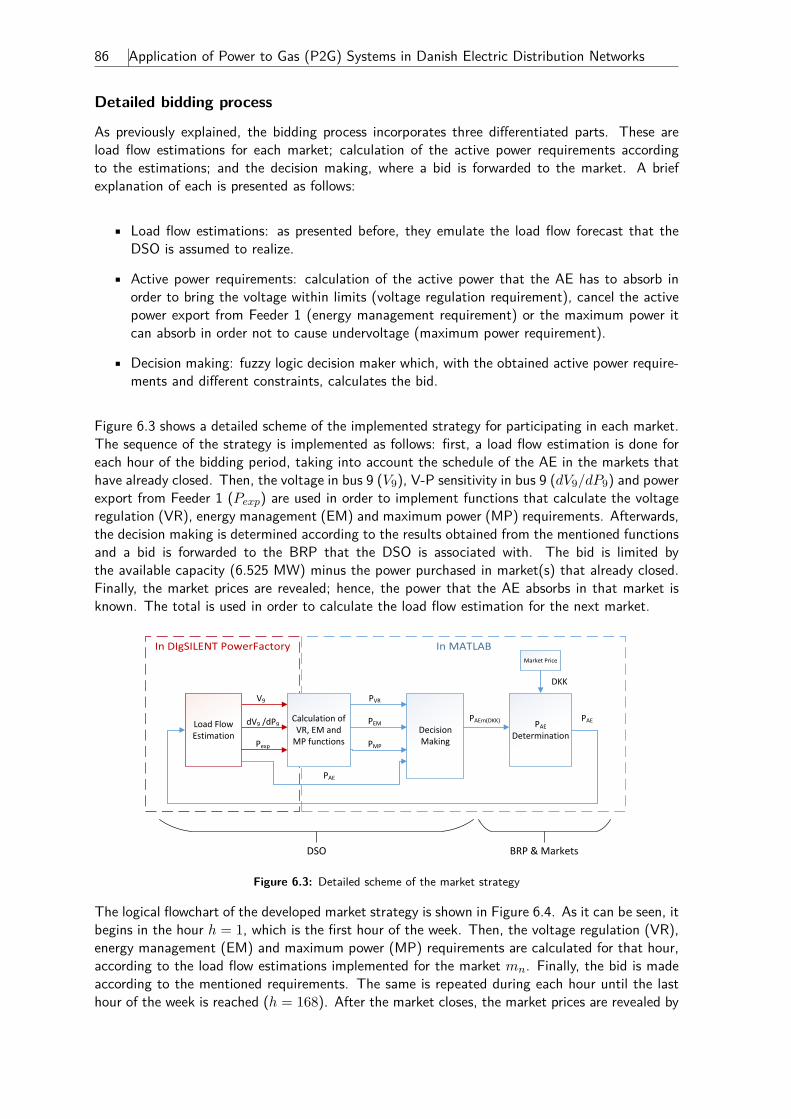
86 Application of Power to Gas (P2G) Systems in Danish Electric Distribution Networks
Detailed bidding process
As previously explained, the bidding process incorporates three differentiated parts. These areload flow estimations for each market; calculation of the active power requirements accordingto the estimations; and the decision making, where a bid is forwarded to the market. A briefexplanation of each is presented as follows:
• Load flow estimations: as presented before, they emulate the load flow forecast that theDSO is assumed to realize.
• Active power requirements: calculation of the active power that the AE has to absorb inorder to bring the voltage within limits (voltage regulation requirement), cancel the activepower export from Feeder 1 (energy management requirement) or the maximum power itcan absorb in order not to cause undervoltage (maximum power requirement).
• Decision making: fuzzy logic decision maker which, with the obtained active power require-ments and different constraints, calculates the bid.
Figure 6.3 shows a detailed scheme of the implemented strategy for participating in each market.The sequence of the strategy is implemented as follows: first, a load flow estimation is done foreach hour of the bidding period, taking into account the schedule of the AE in the markets thathave already closed. Then, the voltage in bus 9 (V9), V-P sensitivity in bus 9 (dV9/dP9) and powerexport from Feeder 1 (Pexp) are used in order to implement functions that calculate the voltageregulation (VR), energy management (EM) and maximum power (MP) requirements. Afterwards,the decision making is determined according to the results obtained from the mentioned functionsand a bid is forwarded to the BRP that the DSO is associated with. The bid is limited bythe available capacity (6.525 MW) minus the power purchased in market(s) that already closed.Finally, the market prices are revealed; hence, the power that the AE absorbs in that market isknown. The total is used in order to calculate the load flow estimation for the next market.
Calculation of VR, EM and MP functions
Decision Making
PAE Determination
Market Price
PAE PAEm(DKK)
PVR
PEM
PMP
V9
Pexp
Load Flow Estimation
dV9 /dP9
DKK
PAE
DSO BRP & Markets
Figure 6.3: Detailed scheme of the market strategy
The logical flowchart of the developed market strategy is shown in Figure 6.4. As it can be seen, itbegins in the hour h = 1, which is the first hour of the week. Then, the voltage regulation (VR),energy management (EM) and maximum power (MP) requirements are calculated for that hour,according to the load flow estimations implemented for the market mn. Finally, the bid is madeaccording to the mentioned requirements. The same is repeated during each hour until the lasthour of the week is reached (h = 168). After the market closes, the market prices are revealed by
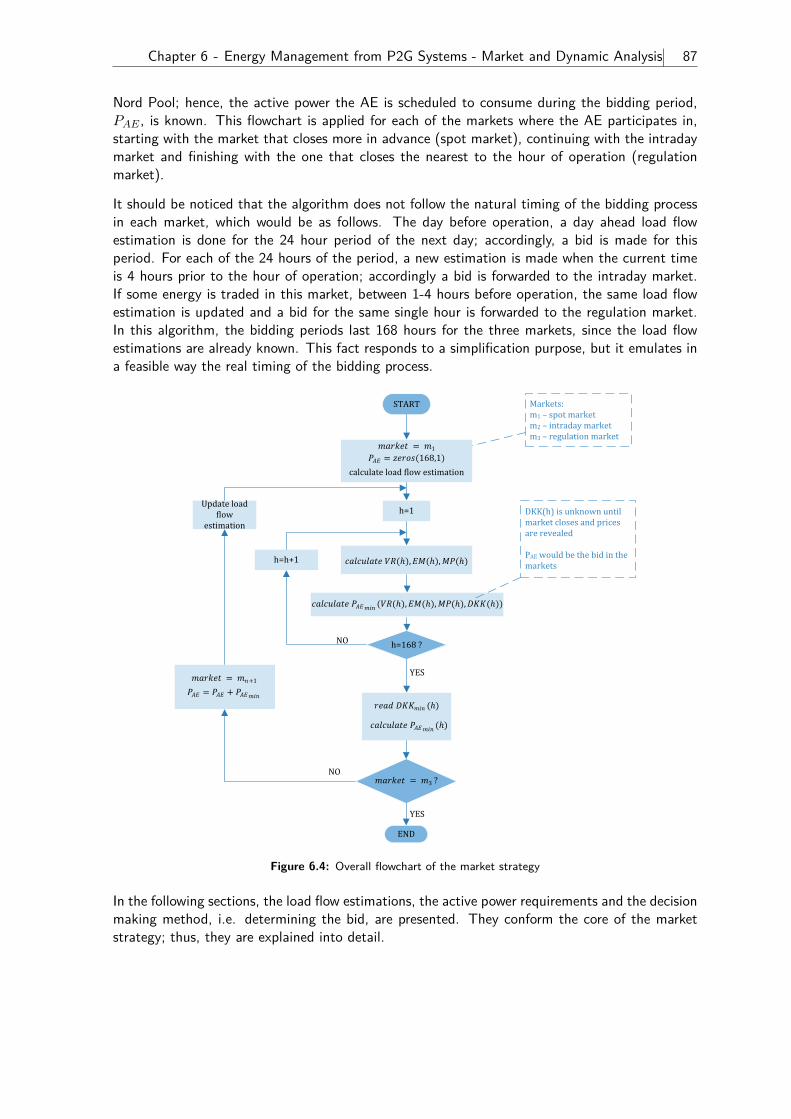
Chapter 6 - Energy Management from P2G Systems - Market and Dynamic Analysis 87
Nord Pool; hence, the active power the AE is scheduled to consume during the bidding period,PAE , is known. This flowchart is applied for each of the markets where the AE participates in,starting with the market that closes more in advance (spot market), continuing with the intradaymarket and finishing with the one that closes the nearest to the hour of operation (regulationmarket).
It should be noticed that the algorithm does not follow the natural timing of the bidding processin each market, which would be as follows. The day before operation, a day ahead load flowestimation is done for the 24 hour period of the next day; accordingly, a bid is made for thisperiod. For each of the 24 hours of the period, a new estimation is made when the current timeis 4 hours prior to the hour of operation; accordingly a bid is forwarded to the intraday market.If some energy is traded in this market, between 1-4 hours before operation, the same load flowestimation is updated and a bid for the same single hour is forwarded to the regulation market.In this algorithm, the bidding periods last 168 hours for the three markets, since the load flowestimations are already known. This fact responds to a simplification purpose, but it emulates ina feasible way the real timing of the bidding process.
START
h=1
h=168?
h=h+1
NO
calculateloadflowestimation
1
168,1
, ,
3 ?NO
YES
END
1
Updateloadflow
estimation
YES
, , ,
Markets:m1–spotmarketm2–intradaymarketm3–regulationmarket
DKK(h)isunknownuntilmarketclosesandpricesarerevealed
PAEwouldbethebidinthemarkets
Figure 6.4: Overall flowchart of the market strategy
In the following sections, the load flow estimations, the active power requirements and the decisionmaking method, i.e. determining the bid, are presented. They conform the core of the marketstrategy; thus, they are explained into detail.
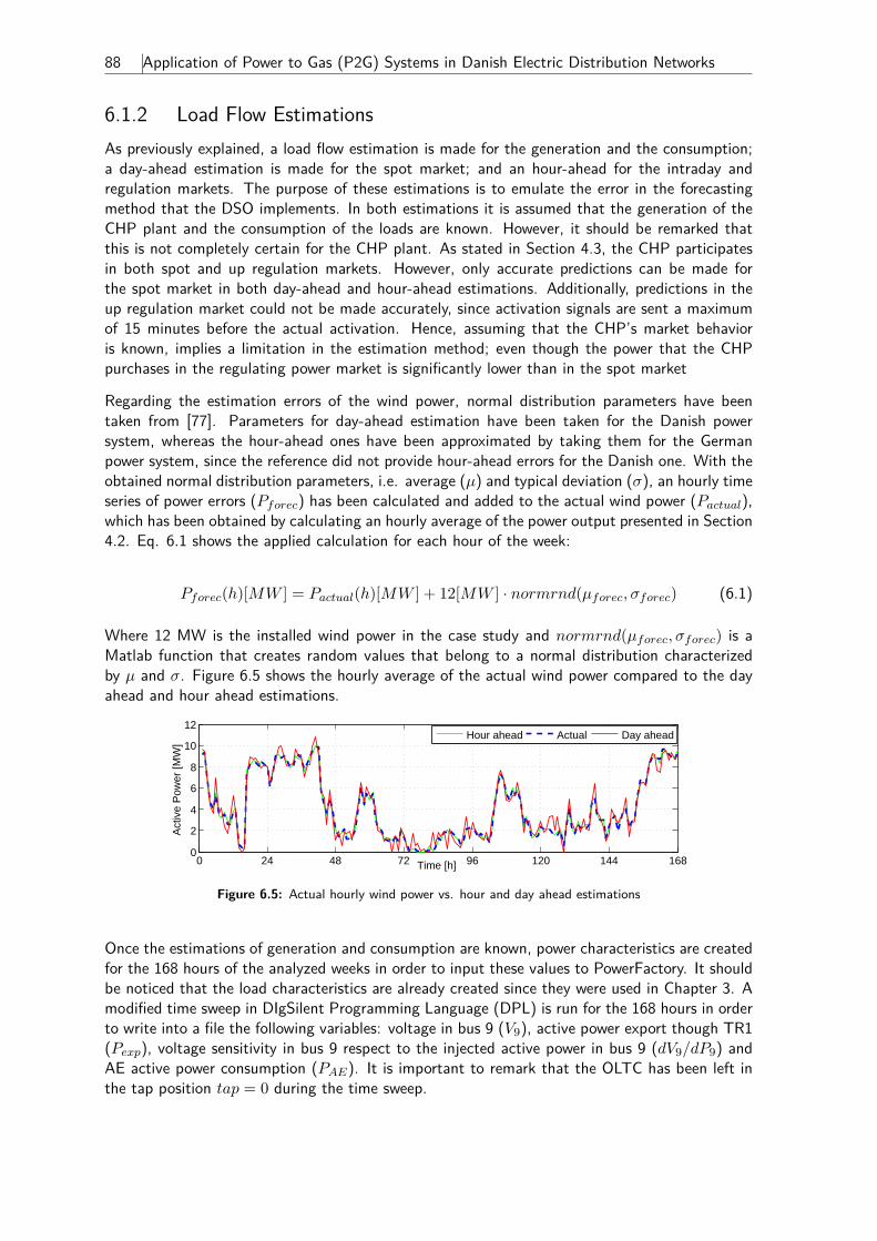
88 Application of Power to Gas (P2G) Systems in Danish Electric Distribution Networks
6.1.2 Load Flow EstimationsAs previously explained, a load flow estimation is made for the generation and the consumption;a day-ahead estimation is made for the spot market; and an hour-ahead for the intraday andregulation markets. The purpose of these estimations is to emulate the error in the forecastingmethod that the DSO implements. In both estimations it is assumed that the generation of theCHP plant and the consumption of the loads are known. However, it should be remarked thatthis is not completely certain for the CHP plant. As stated in Section 4.3, the CHP participatesin both spot and up regulation markets. However, only accurate predictions can be made forthe spot market in both day-ahead and hour-ahead estimations. Additionally, predictions in theup regulation market could not be made accurately, since activation signals are sent a maximumof 15 minutes before the actual activation. Hence, assuming that the CHP’s market behavioris known, implies a limitation in the estimation method; even though the power that the CHPpurchases in the regulating power market is significantly lower than in the spot market
Regarding the estimation errors of the wind power, normal distribution parameters have beentaken from [77]. Parameters for day-ahead estimation have been taken for the Danish powersystem, whereas the hour-ahead ones have been approximated by taking them for the Germanpower system, since the reference did not provide hour-ahead errors for the Danish one. With theobtained normal distribution parameters, i.e. average (µ) and typical deviation (σ), an hourly timeseries of power errors (Pforec) has been calculated and added to the actual wind power (Pactual),which has been obtained by calculating an hourly average of the power output presented in Section4.2. Eq. 6.1 shows the applied calculation for each hour of the week:
Pforec(h)[MW ] = Pactual(h)[MW ] + 12[MW ] · normrnd(µforec, σforec) (6.1)
Where 12 MW is the installed wind power in the case study and normrnd(µforec, σforec) is aMatlab function that creates random values that belong to a normal distribution characterizedby µ and σ. Figure 6.5 shows the hourly average of the actual wind power compared to the dayahead and hour ahead estimations.
0 24 48 72 96 120 144 1680
2
4
6
8
10
12
Time [h]
Act
ive
Pow
er [M
W]
Hour ahead Actual Day ahead
Figure 6.5: Actual hourly wind power vs. hour and day ahead estimations
Once the estimations of generation and consumption are known, power characteristics are createdfor the 168 hours of the analyzed weeks in order to input these values to PowerFactory. It shouldbe noticed that the load characteristics are already created since they were used in Chapter 3. Amodified time sweep in DIgSilent Programming Language (DPL) is run for the 168 hours in orderto write into a file the following variables: voltage in bus 9 (V9), active power export though TR1(Pexp), voltage sensitivity in bus 9 respect to the injected active power in bus 9 (dV9/dP9) andAE active power consumption (PAE). It is important to remark that the OLTC has been left inthe tap position tap = 0 during the time sweep.
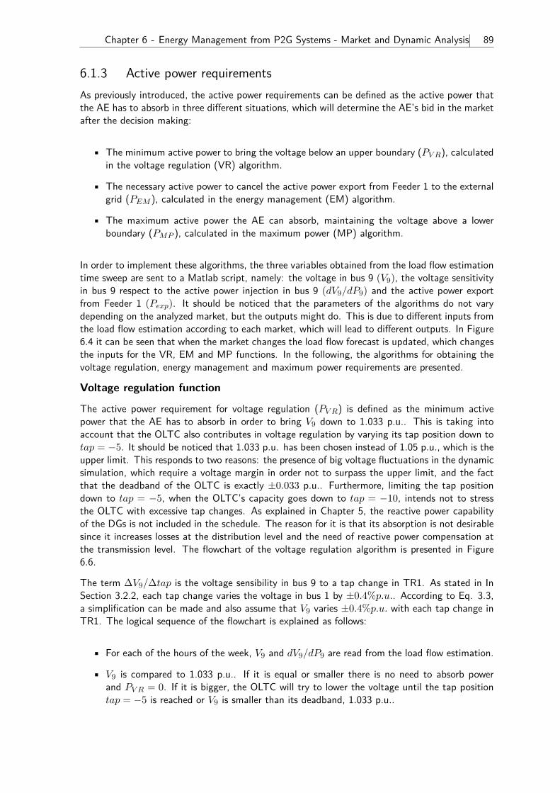
Chapter 6 - Energy Management from P2G Systems - Market and Dynamic Analysis 89
6.1.3 Active power requirementsAs previously introduced, the active power requirements can be defined as the active power thatthe AE has to absorb in three different situations, which will determine the AE’s bid in the marketafter the decision making:
• The minimum active power to bring the voltage below an upper boundary (PV R), calculatedin the voltage regulation (VR) algorithm.
• The necessary active power to cancel the active power export from Feeder 1 to the externalgrid (PEM ), calculated in the energy management (EM) algorithm.
• The maximum active power the AE can absorb, maintaining the voltage above a lowerboundary (PMP ), calculated in the maximum power (MP) algorithm.
In order to implement these algorithms, the three variables obtained from the load flow estimationtime sweep are sent to a Matlab script, namely: the voltage in bus 9 (V9), the voltage sensitivityin bus 9 respect to the active power injection in bus 9 (dV9/dP9) and the active power exportfrom Feeder 1 (Pexp). It should be noticed that the parameters of the algorithms do not varydepending on the analyzed market, but the outputs might do. This is due to different inputs fromthe load flow estimation according to each market, which will lead to different outputs. In Figure6.4 it can be seen that when the market changes the load flow forecast is updated, which changesthe inputs for the VR, EM and MP functions. In the following, the algorithms for obtaining thevoltage regulation, energy management and maximum power requirements are presented.
Voltage regulation function
The active power requirement for voltage regulation (PV R) is defined as the minimum activepower that the AE has to absorb in order to bring V9 down to 1.033 p.u.. This is taking intoaccount that the OLTC also contributes in voltage regulation by varying its tap position down totap = −5. It should be noticed that 1.033 p.u. has been chosen instead of 1.05 p.u., which is theupper limit. This responds to two reasons: the presence of big voltage fluctuations in the dynamicsimulation, which require a voltage margin in order not to surpass the upper limit, and the factthat the deadband of the OLTC is exactly ±0.033 p.u.. Furthermore, limiting the tap positiondown to tap = −5, when the OLTC’s capacity goes down to tap = −10, intends not to stressthe OLTC with excessive tap changes. As explained in Chapter 5, the reactive power capabilityof the DGs is not included in the schedule. The reason for it is that its absorption is not desirablesince it increases losses at the distribution level and the need of reactive power compensation atthe transmission level. The flowchart of the voltage regulation algorithm is presented in Figure6.6.
The term ∆V9/∆tap is the voltage sensibility in bus 9 to a tap change in TR1. As stated in InSection 3.2.2, each tap change varies the voltage in bus 1 by ±0.4%p.u.. According to Eq. 3.3,a simplification can be made and also assume that V9 varies ±0.4%p.u. with each tap change inTR1. The logical sequence of the flowchart is explained as follows:
• For each of the hours of the week, V9 and dV9/dP9 are read from the load flow estimation.
• V9 is compared to 1.033 p.u.. If it is equal or smaller there is no need to absorb powerand PV R = 0. If it is bigger, the OLTC will try to lower the voltage until the tap positiontap = −5 is reached or V9 is smaller than its deadband, 1.033 p.u..
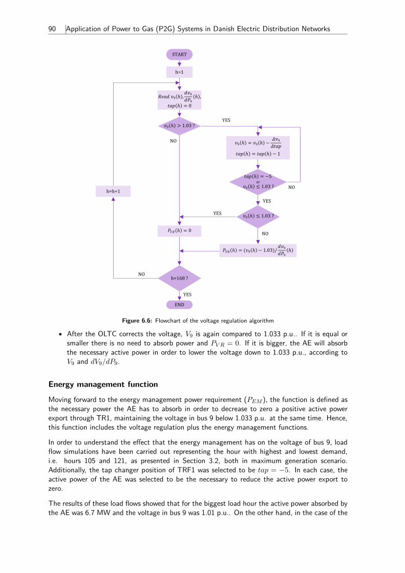
90 Application of Power to Gas (P2G) Systems in Danish Electric Distribution Networks
START
h=1
or
h=168?
END
h=h+1
1
9 99
5
9 1.03 ?
9 1.03 ?
YES
NO
YES
NO
NO
YES
YES
9 1.03 / 9
9
9 , 9
9,
0
9 1.03 ?
NO
0
Figure 6.6: Flowchart of the voltage regulation algorithm
• After the OLTC corrects the voltage, V9 is again compared to 1.033 p.u.. If it is equal orsmaller there is no need to absorb power and PV R = 0. If it is bigger, the AE will absorbthe necessary active power in order to lower the voltage down to 1.033 p.u., according toV9 and dV9/dP9.
Energy management function
Moving forward to the energy management power requirement (PEM ), the function is defined asthe necessary power the AE has to absorb in order to decrease to zero a positive active powerexport through TR1, maintaining the voltage in bus 9 below 1.033 p.u. at the same time. Hence,this function includes the voltage regulation plus the energy management functions.
In order to understand the effect that the energy management has on the voltage of bus 9, loadflow simulations have been carried out representing the hour with highest and lowest demand,i.e. hours 105 and 121, as presented in Section 3.2, both in maximum generation scenario.Additionally, the tap changer position of TRF1 was selected to be tap = −5. In each case, theactive power of the AE was selected to be the necessary to reduce the active power export tozero.
The results of these load flows showed that for the biggest load hour the active power absorbed bythe AE was 6.7 MW and the voltage in bus 9 was 1.01 p.u.. On the other hand, in the case of the
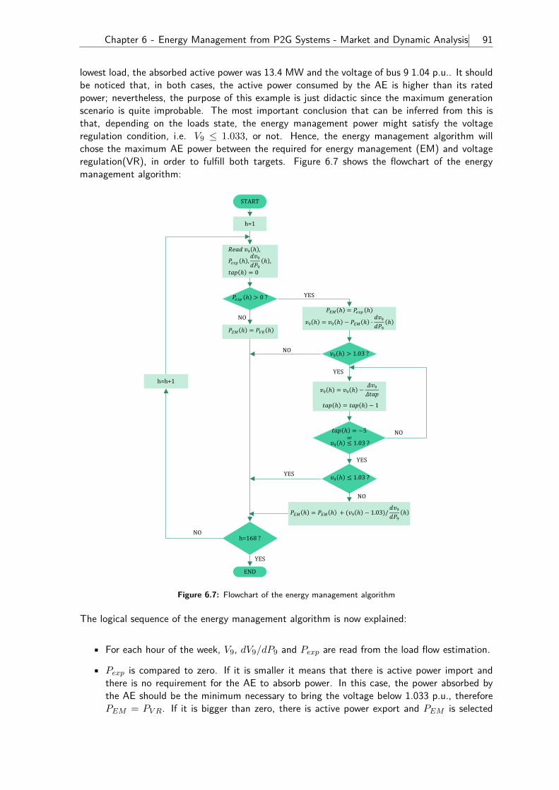
Chapter 6 - Energy Management from P2G Systems - Market and Dynamic Analysis 91
lowest load, the absorbed active power was 13.4 MW and the voltage of bus 9 1.04 p.u.. It shouldbe noticed that, in both cases, the active power consumed by the AE is higher than its ratedpower; nevertheless, the purpose of this example is just didactic since the maximum generationscenario is quite improbable. The most important conclusion that can be inferred from this isthat, depending on the loads state, the energy management power might satisfy the voltageregulation condition, i.e. V9 ≤ 1.033, or not. Hence, the energy management algorithm willchose the maximum AE power between the required for energy management (EM) and voltageregulation(VR), in order to fulfill both targets. Figure 6.7 shows the flowchart of the energymanagement algorithm:
START
h=1
or
h=168?
END
h=h+1
9 ,
, 9
9,
0
0 ?
9 99
9
9 1.03?
1
9 99
5
9 1.03 ?
9 1.03 ?
9 1.03 / 9
9
YES
NO
YES
YES
NO
NO
NO
YES
YES
NO
Figure 6.7: Flowchart of the energy management algorithm
The logical sequence of the energy management algorithm is now explained:
• For each hour of the week, V9, dV9/dP9 and Pexp are read from the load flow estimation.
• Pexp is compared to zero. If it is smaller it means that there is active power import andthere is no requirement for the AE to absorb power. In this case, the power absorbed bythe AE should be the minimum necessary to bring the voltage below 1.033 p.u., thereforePEM = PV R. If it is bigger than zero, there is active power export and PEM is selected
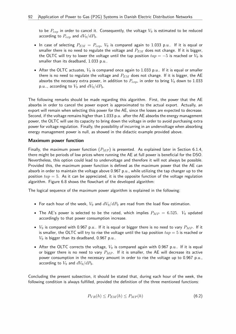
92 Application of Power to Gas (P2G) Systems in Danish Electric Distribution Networks
to be Pexp in order to cancel it. Consequently, the voltage V9 is estimated to be reducedaccording to Pexp and dV9/dP9.
• In case of selecting PEM = Pexp, V9 is compared again to 1.033 p.u.. If it is equal orsmaller there is no need to regulate the voltage and PEM does not change. If it is bigger,the OLTC will try to lower the voltage until the tap position tap = −5 is reached or V9 issmaller than its deadband, 1.033 p.u..
• After the OLTC actuates, V9 is compared once again to 1.033 p.u.. If it is equal or smallerthere is no need to regulate the voltage and PEM does not change. If it is bigger, the AEabsorbs the necessary extra power, in addition to Pexp, in order to bring V9 down to 1.033p.u.., according to V9 and dV9/dP9.
The following remarks should be made regarding this algorithm. First, the power that the AEabsorbs in order to cancel the power export is approximated to the actual export. Actually, anexport will remain when selecting this power for the AE, since the losses are expected to decrease.Second, if the voltage remains higher than 1.033 p.u. after the AE absorbs the energy managementpower, the OLTC will use its capacity to bring down the voltage in order to avoid purchasing extrapower for voltage regulation. Finally, the possibility of incurring in an undervoltage when absorbingenergy management power is null, as showed in the didactic example provided above.
Maximum power function
Finally, the maximum power function (PMP ) is presented. As explained later in Section 6.1.4,there might be periods of low prices where running the AE at full power is beneficial for the DSO.Nevertheless, this option could lead to undervoltage and therefore it will not always be possible.Provided this, the maximum power function is defined as the maximum power that the AE canabsorb in order to maintain the voltage above 0.967 p.u., while utilizing the tap changer up to theposition tap = 5. As it can be appreciated, it is the opposite function of the voltage regulationalgorithm. Figure 6.8 shows the flowchart of the developed algorithm:
The logical sequence of the maximum power algorithm is explained in the following:
• For each hour of the week, V9 and dV9/dP9 are read from the load flow estimation.
• The AE’s power is selected to be the rated, which implies PMP = 6.525. V9 updatedaccordingly to that power consumption increase.
• V9 is compared with 0.967 p.u.. If it is equal or bigger there is no need to vary PMP . If itis smaller, the OLTC will try to rise the voltage until the tap position tap = 5 is reached orV9 is bigger than its deadband, 0.967 p.u..
• After the OLTC corrects the voltage, V9 is compared again with 0.967 p.u.. If it is equalor bigger there is no need to vary PMP . If it is smaller, the AE will decrease its activepower consumption in the necessary amount in order to rise the voltage up to 0.967 p.u.,according to V9 and dV9/dP9.
Concluding the present subsection, it should be stated that, during each hour of the week, thefollowing condition is always fulfilled, provided the definition of the three mentioned functions:
PV R(h) ≤ PEM (h) ≤ PMP (h) (6.2)
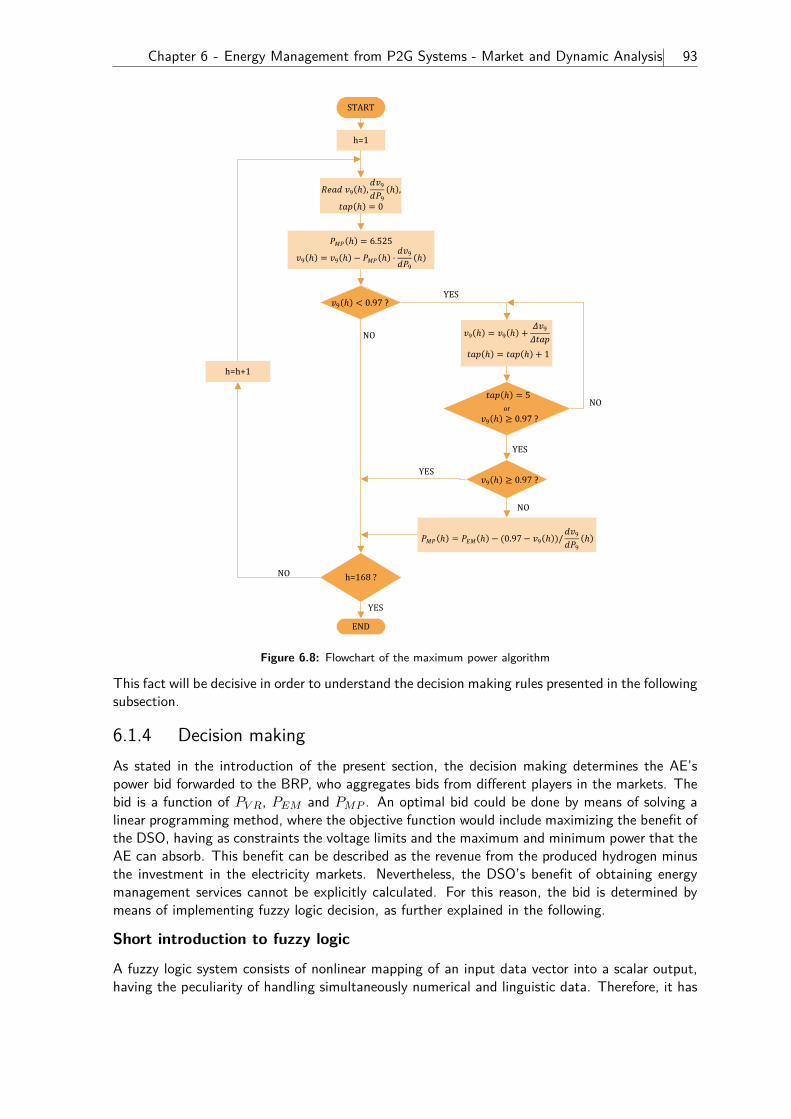
Chapter 6 - Energy Management from P2G Systems - Market and Dynamic Analysis 93
START
h=1
h=168?
END
h=h+1
9 , 9
9,
0
9 0.97 ?
YES
YES
9 0.97 ?
6.525
9 99
9
or
5
9 0.97 ?
YES
9 99
1
NO
0.97 9 / 9
9
NO
NO
YES
NO
Figure 6.8: Flowchart of the maximum power algorithm
This fact will be decisive in order to understand the decision making rules presented in the followingsubsection.
6.1.4 Decision makingAs stated in the introduction of the present section, the decision making determines the AE’spower bid forwarded to the BRP, who aggregates bids from different players in the markets. Thebid is a function of PV R, PEM and PMP . An optimal bid could be done by means of solving alinear programming method, where the objective function would include maximizing the benefit ofthe DSO, having as constraints the voltage limits and the maximum and minimum power that theAE can absorb. This benefit can be described as the revenue from the produced hydrogen minusthe investment in the electricity markets. Nevertheless, the DSO’s benefit of obtaining energymanagement services cannot be explicitly calculated. For this reason, the bid is determined bymeans of implementing fuzzy logic decision, as further explained in the following.
Short introduction to fuzzy logic
A fuzzy logic system consists of nonlinear mapping of an input data vector into a scalar output,having the peculiarity of handling simultaneously numerical and linguistic data. Therefore, it has
94 Application of Power to Gas (P2G) Systems in Danish Electric Distribution Networks
a great potential for solving problems that are inherently complex to model [78]. In every fuzzylogic system, numerical inputs that belong to linguistic variables are assigned to linguistic termsin a certain degree of truth, normally within the range of [0,1]. For example, a spot price of245 DKK/MWh can defined as 0.5 medium price and 0.5 high price. In this case, the price isthe linguistic variable, high and medium are the linguistic terms and 0.5 is the membership µi.Membership functions are the responsible to convert the numerical prices into fuzzy ones, in theprocess known as fuzzification. The next step is converting the fuzzy inputs to numerical outputby means of IF-ELSE rules. Continuing with the spot price example, the fuzzy rules could bestated as:
"If the spot price is high, then the purchased power is 1MW"
"If the spot price is medium, then the purchased power is 2MW"
In order to obtain a numerical output, a defuzzification is to be made. Normally, it is done byusing the center of gravity method, shown in Eq. 6.3.
U =∑in=1 µ(ui) · ui∑in=1 µ(ui)
(6.3)
Where u is the output and µ(ui) is the membership of each variable ui. Therefore, for the previousexample, the purchased power (P ) would be calculated as described in Eq. 6.4.
P = 0.5 · 1 + 0.5 · 21 = 1.5MW (6.4)
It should be noticed that the fuzzy rules normally assign fuzzy outputs to the fuzzy inputs, insteadof numerical outputs as it is stated in the example. Nevertheless, choosing directly the numericaloutput turns out to be a shortcut in the method and it fits better with the determination of theAE’s power bid. The structure of a typical fuzzy logic system can be observed in Figure 6.9.
A Short Fuzzy Logic Tutorial
April 8, 2010
The purpose of this tutorial is to give a brief information about fuzzy logicsystems. The tutorial is prepared based on the studies [2] and [1]. For furtherinformation on fuzzy logic, the reader is directed to these studies.
A fuzzy logic system (FLS) can be defined as the nonlinear mapping of aninput data set to a scalar output data [2]. A FLS consists of four main parts:fuzzifier, rules, inference engine, and defuzzifier. These components and thegeneral architecture of a FLS is shown in Figure 1.
Figure 1: A Fuzzy Logic System.
The process of fuzzy logic is explained in Algorithm 1: Firstly, a crisp setof input data are gathered and converted to a fuzzy set using fuzzy linguisticvariables, fuzzy linguistic terms and membership functions. This step is knownas fuzzification. Afterwards, an inference is made based on a set of rules. Lastly,the resulting fuzzy output is mapped to a crisp output using the membershipfunctions, in the defuzzification step.
In order to exemplify the usage of a FLS, consider an air conditioner systemcontrolled by a FLS (Figure 2). The system adjusts the temperature of theroom according to the current temperature of the room and the target value.The fuzzy engine periodically compares the room temperature and the targettemperature, and produces a command to heat or cool the room.
1
Figure 6.9: Typical structure of a fuzzy logic system [79]
The explained fuzzy logic theory has been obtained from [79] and [78], which the reader issuggested to check for further information. In the following the fuzzy logic system is presentedfor the case study purpose.
Fuzzy logic decision making
The numerical input values for the studied fuzzy logic system are the market prices. The differentfuzzy terms assigned to the market price are low, medium and high. The membership functions
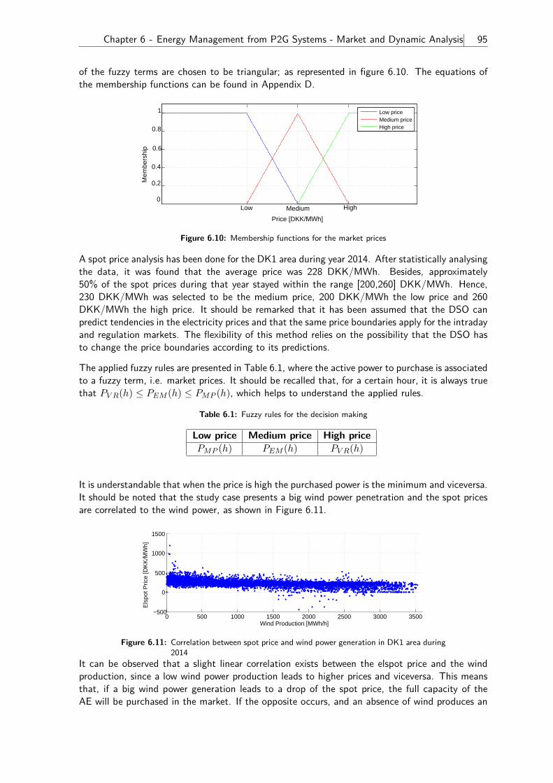
Chapter 6 - Energy Management from P2G Systems - Market and Dynamic Analysis 95
of the fuzzy terms are chosen to be triangular; as represented in figure 6.10. The equations ofthe membership functions can be found in Appendix D.
Low Medium High
0.2
0.4
0.6
0.8
1
Price [DKK/MWh]
Mem
bers
hip
0
Low priceMedium priceHigh price
Figure 6.10: Membership functions for the market prices
A spot price analysis has been done for the DK1 area during year 2014. After statistically analysingthe data, it was found that the average price was 228 DKK/MWh. Besides, approximately50% of the spot prices during that year stayed within the range [200,260] DKK/MWh. Hence,230 DKK/MWh was selected to be the medium price, 200 DKK/MWh the low price and 260DKK/MWh the high price. It should be remarked that it has been assumed that the DSO canpredict tendencies in the electricity prices and that the same price boundaries apply for the intradayand regulation markets. The flexibility of this method relies on the possibility that the DSO hasto change the price boundaries according to its predictions.
The applied fuzzy rules are presented in Table 6.1, where the active power to purchase is associatedto a fuzzy term, i.e. market prices. It should be recalled that, for a certain hour, it is always truethat PV R(h) ≤ PEM (h) ≤ PMP (h), which helps to understand the applied rules.
Table 6.1: Fuzzy rules for the decision making
Low price Medium price High pricePMP (h) PEM (h) PV R(h)
It is understandable that when the price is high the purchased power is the minimum and viceversa.It should be noted that the study case presents a big wind power penetration and the spot pricesare correlated to the wind power, as shown in Figure 6.11.
0 500 1000 1500 2000 2500 3000 3500−500
0
500
1000
1500
Wind Production [MWh/h]
Els
pot P
rice
[DK
K/MWh]
Figure 6.11: Correlation between spot price and wind power generation in DK1 area during2014
It can be observed that a slight linear correlation exists between the elspot price and the windproduction, since a low wind power production leads to higher prices and viceversa. This meansthat, if a big wind power generation leads to a drop of the spot price, the full capacity of theAE will be purchased in the market. If the opposite occurs, and an absence of wind produces an
96 Application of Power to Gas (P2G) Systems in Danish Electric Distribution Networks
increase of the spot price, the purchased power will be zero since the absence of wind will notproduce overvoltage. Nevertheless, the method is prepared to withstand no correlation betweenwind power and market price since the OLTC provides flexibility in the voltage regulation.
For the defuzzification process, the center of gravity method is applied and the power bid isdefined as in Eq. 6.5. It should be noticed that the memberships µLow, µMed and µHigh varywith the price according to Figure 6.10. In the following the constraints applied to the output ofthe fuzzy logic decision maker are presented.
PAE(h) = µLow · PMP (h) + µMed · PEM (h) + µHigh · PV R(h) (6.5)
AE’s power constraints
In the following, the power constraints imposed to the AE’s power consumption are presented.Firstly, the temperature constraint is analyzed and subsequently, the constraints are applied tothe results obtained in the fuzzy logic decision maker.
As stated in the conclusions of Chapter 4, the electrolyzer requires approximately 132 minutesto reach full power from cold start. This limitation might compromise the participation of theelectrolyzer in the different markets, not reaching the scheduled active power set-point. In orderto avoid this, three different solutions are proposed:
• Estimate the evolution of the temperature and limit the purchase of power for the operationhour n+ 1 according to the temperature of the device at the end of the hour n.
• Use additional sources of heat in order to maintain the temperature at the rated value, i.e.80°C.
• Operate the electrolyzer at the minimum power so its temperature does not go below 80°C.
The first proposed solution has a complex execution, whereas the second does not appear in theliterature and might present technical issues in its implementation; therefore, the last proposedsolution is implemented in the present work.
It was found out that giving the electrolyzer module a set-point above 0.053 MW (0.067 MWincluding compression power), the temperature remained constant at 80°C. Hence, a minimumof 1.005 MW, accounting for the 15 units, will be purchased in the spot market in order to keepthe temperature at the rated and assure full regulation capability. However, it should be noticedthat there is a minimum load requirement in order to produce hydrogen without compromisingits purity. In [47] this minimum stated to be within the range 15-20%. The calculated minimumfor the temperature limitation is of 14.9%; hence, it is assumed that the produced hydrogen willnot possess any quality issue.
Once the fuzzy logic decision maker calculates the active power for each of the markets, upperand lower limitations have to be applied to the obtained values:
• For the spot market, the upper limitation is the rated capacity of the AE (6.525 MW)whereas the lower is the minimum power in order to maintain the AE’s temperature at80°C (1.005 MW).
• For the intraday market, the upper limitation is the difference between the rated capacityand the power traded in the spot market, whereas the lower capacity is zero.
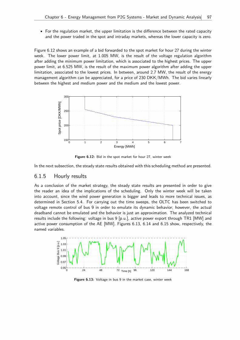
Chapter 6 - Energy Management from P2G Systems - Market and Dynamic Analysis 97
• For the regulation market, the upper limitation is the difference between the rated capacityand the power traded in the spot and intraday markets, whereas the lower capacity is zero.
Figure 6.12 shows an example of a bid forwarded to the spot market for hour 27 during the winterweek. The lower power limit, at 1.005 MW, is the result of the voltage regulation algorithmafter adding the minimum power limitation, which is associated to the highest prices. The upperpower limit, at 6.525 MW, is the result of the maximum power algorithm after adding the upperlimitation, associated to the lowest prices. In between, around 2.7 MW, the result of the energymanagement algorithm can be appreciated, for a price of 230 DKK/MWh. The bid varies linearlybetween the highest and medium power and the medium and the lowest power.
0 1 2 3 4 5 6 7150
200
250
300
Energy [MWh]
Spo
t pric
e [D
KK/MWh]
Figure 6.12: Bid in the spot market for hour 27, winter week
In the next subsection, the steady state results obtained with this scheduling method are presented.
6.1.5 Hourly resultsAs a conclusion of the market strategy, the steady state results are presented in order to givethe reader an idea of the implications of the scheduling. Only the winter week will be takeninto account, since the wind power generation is bigger and leads to more technical issues, asdetermined in Section 5.4. For carrying out the time sweeps, the OLTC has been switched tovoltage remote control of bus 9 in order to emulate its dynamic behavior; however, the actualdeadband cannot be emulated and the behavior is just an approximation. The analyzed technicalresults include the following: voltage in bus 9 [p.u.], active power export through TR1 [MW] andactive power consumption of the AE [MW]. Figures 6.13, 6.14 and 6.15 show, respectively, thenamed variables.
0 24 48 72 96 120 144 1680.95
0.97
0.99
1.01
1.03
1.05
Time [h]
Vol
tage
Bus
9 [p
.u.]
Figure 6.13: Voltage in bus 9 in the market case, winter week
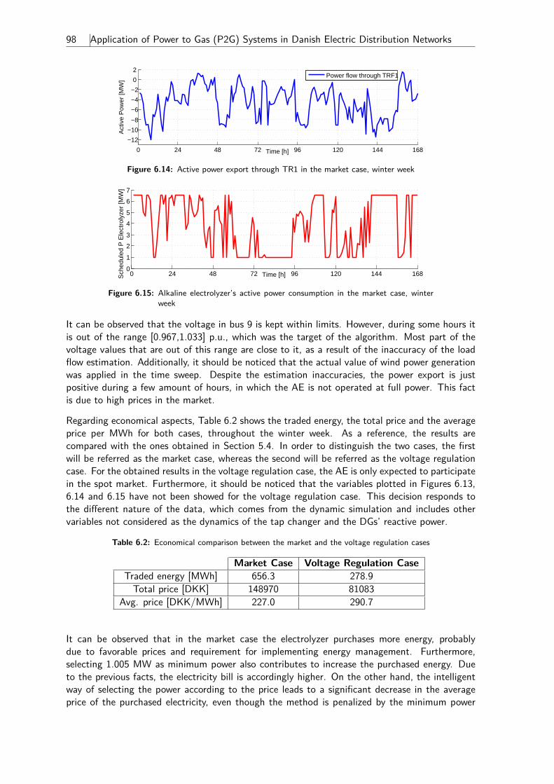
98 Application of Power to Gas (P2G) Systems in Danish Electric Distribution Networks
0 24 48 72 96 120 144 168
−12
−10
−8
−6
−4
−2
0
2
Time [h]
Act
ive
Pow
er [M
W]
Power flow through TRF1
Figure 6.14: Active power export through TR1 in the market case, winter week
0 24 48 72 96 120 144 1680
1
2
3
4
5
6
7
Time [h]Sch
edul
ed P
Ele
ctro
lyze
r [M
W]
Figure 6.15: Alkaline electrolyzer’s active power consumption in the market case, winterweek
It can be observed that the voltage in bus 9 is kept within limits. However, during some hours itis out of the range [0.967,1.033] p.u., which was the target of the algorithm. Most part of thevoltage values that are out of this range are close to it, as a result of the inaccuracy of the loadflow estimation. Additionally, it should be noticed that the actual value of wind power generationwas applied in the time sweep. Despite the estimation inaccuracies, the power export is justpositive during a few amount of hours, in which the AE is not operated at full power. This factis due to high prices in the market.
Regarding economical aspects, Table 6.2 shows the traded energy, the total price and the averageprice per MWh for both cases, throughout the winter week. As a reference, the results arecompared with the ones obtained in Section 5.4. In order to distinguish the two cases, the firstwill be referred as the market case, whereas the second will be referred as the voltage regulationcase. For the obtained results in the voltage regulation case, the AE is only expected to participatein the spot market. Furthermore, it should be noticed that the variables plotted in Figures 6.13,6.14 and 6.15 have not been showed for the voltage regulation case. This decision responds tothe different nature of the data, which comes from the dynamic simulation and includes othervariables not considered as the dynamics of the tap changer and the DGs’ reactive power.
Table 6.2: Economical comparison between the market and the voltage regulation cases
Market Case Voltage Regulation CaseTraded energy [MWh] 656.3 278.9Total price [DKK] 148970 81083
Avg. price [DKK/MWh] 227.0 290.7
It can be observed that in the market case the electrolyzer purchases more energy, probablydue to favorable prices and requirement for implementing energy management. Furthermore,selecting 1.005 MW as minimum power also contributes to increase the purchased energy. Dueto the previous facts, the electricity bill is accordingly higher. On the other hand, the intelligentway of selecting the power according to the price leads to a significant decrease in the averageprice of the purchased electricity, even though the method is penalized by the minimum power
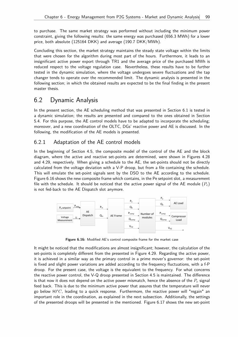
Chapter 6 - Energy Management from P2G Systems - Market and Dynamic Analysis 99
to purchase. The same market strategy was performed without including the minimum powerconstraint, giving the following results: the same energy was purchased (656.3 MWh) for a lowerprice, both absolute (125164 DKK) and average (190.7 DKK/MWh).
Concluding this section, the market strategy maintains the steady state voltage within the limitsthat were chosen for the algorithm during most part of the hours. Furthermore, it leads to aninsignificant active power export through TR1 and the average price of the purchased MWh isreduced respect to the voltage regulation case. Nevertheless, these results have to be furthertested in the dynamic simulation, where the voltage undergoes severe fluctuations and the tapchanger tends to operate over the recommended limit. The dynamic analysis is presented in thefollowing section; in which the obtained results are expected to be the final finding in the presentmaster thesis.
6.2 Dynamic AnalysisIn the present section, the AE scheduling method that was presented in Section 6.1 is tested ina dynamic simulation; the results are presented and compared to the ones obtained in Section5.4. For this purpose, the AE control models have to be adapted to incorporate the scheduling;moreover, and a new coordination of the OLTC, DGs’ reactive power and AE is discussed. In thefollowing, the modification of the AE models is presented.
6.2.1 Adaptation of the AE control modelsIn the beginning of Section 4.5, the composite model of the control of the AE and the blockdiagram, where the active and reactive set-points are determined, were shown in Figures 4.28and 4.29, respectively. When giving a schedule to the AE, the set-points should not be directlycalculated from the voltage deviation with a V-P droop, but from a file containing the schedule.This will emulate the set-point signals sent by the DSO to the AE according to the schedule.Figure 6.16 shows the new composite frame which contains, in the Pe setpoint slot, a measurementfile with the schedule. It should be noticed that the active power signal of the AE module (Pe)is not fed-back to the AE Dispatch slot anymore.
Pcomp
Qcomp
AE Dispatch
AE Load
Pin
QinVoltage Measurement
Pe
AE Frame
Qe
Number of modules
Qe
VH2 VH2
Pe
Pcomp
Qcomp
CompressorLoad
Pe setpointPsetp
U
Figure 6.16: Modified AE’s control composite frame for the market case
It might be noticed that the modifications are almost insignificant; however, the calculation of theset-points is completely different from the presented in Figure 4.29. Regarding the active power,it is achieved in a similar way as the primary control in a prime mover’s governor: the set-pointis fixed and slight power variations are added according to the frequency fluctuations, with a f-Pdroop. For the present case, the voltage is the equivalent to the frequency. For what concernsthe reactive power control, the V-Q droop presented in Section 4.5 is maintained. The differenceis that now it does not depend on the active power mismatch, hence the absence of the Pe signalfeed back. This is due to the minimum active power that assures that the temperature will nevergo below 80°C, leading to a quick response. Furthermore, the reactive power will "regain" animportant role in the coordination, as explained in the next subsection. Additionally, the settingsof the presented droops will be presented in the mentioned. Figure 6.17 shows the new set-point
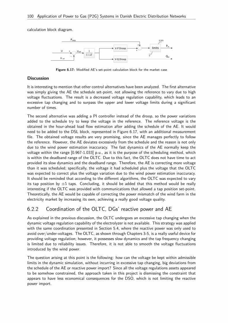
100 Application of Power to Gas (P2G) Systems in Danish Electric Distribution Networks
calculation block diagram.
U ref‐
+U
Pin
Qin
11 sT
Udiff
V‐P Droop
V‐Q Droop
limits
0.355
0
+
+
Psetp
Figure 6.17: Modified AE’s set-point calculation block for the market case
Discussion
It is interesting to mention that other control alternatives have been analyzed. The first alternativewas simply giving the AE the schedule set-point, not allowing the reference to vary due to highvoltage fluctuations. The result is a decreased voltage regulation capability, which leads to anexcessive tap changing and to surpass the upper and lower voltage limits during a significantnumber of times.
The second alternative was adding a PI controller instead of the droop, so the power variationsadded to the schedule try to keep the voltage in the reference. The reference voltage is theobtained in the hour-ahead load flow estimation after adding the schedule of the AE. It wouldneed to be added to the DSL block, represented in Figure 6.17, with an additional measurementfile. The obtained voltage results are very promising, since the AE manages perfectly to followthe reference. However, the AE deviates excessively from the schedule and the reason is not onlydue to the wind power estimation inaccuracy. The fast dynamics of the AE normally keep thevoltage within the range [0.967-1.033] p.u., as it is the purpose of the scheduling method, whichis within the deadband range of the OLTC. Due to this fact, the OLTC does not have time to actprovided its slow dynamics and the deadband range. Therefore, the AE is correcting more voltagethan it was scheduled; specifically, the voltage it had scheduled plus the voltage that the OLTCwas expected to correct plus the voltage variation due to the wind power estimation inaccuracy.It should be reminded that according to the different algorithms, the OLTC was expected to varyits tap position by ±5 taps. Concluding, it should be added that this method would be reallyinteresting if the OLTC was provided with communications that allowed a tap position set-point.Theoretically, the AE would be capable of correcting the power mismatch of the wind farm in theelectricity market by increasing its own, achieving a really good voltage quality.
6.2.2 Coordination of the OLTC, DGs’ reactive power and AEAs explained in the previous discussion, the OLTC undergoes an excessive tap changing when thedynamic voltage regulation capability of the electrolyzer is not available. This strategy was appliedwith the same coordination presented in Section 5.4, where the reactive power was only used toavoid over/under-voltages. The OLTC, as shown through Chapters 3-5, is a really useful device forproviding voltage regulation; however, it possesses slow dynamics and the tap frequency changingis limited due to reliability issues. Therefore, it is not able to smooth the voltage fluctuationsintroduced by the wind power.
The question arising at this point is the following: how can the voltage be kept within admissiblelimits in the dynamic simulation, without incurring in excessive tap changing, big deviations fromthe schedule of the AE or reactive power import? Since all the voltage regulations assets appearedto be somehow constrained, the approach taken in this project is dismissing the constraint thatappears to have less economical consequences for the DSO, which is not limiting the reactivepower import.
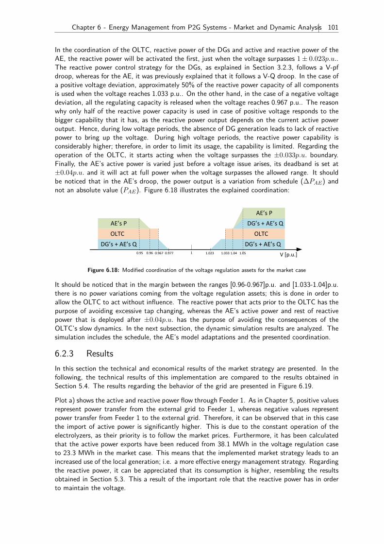
Chapter 6 - Energy Management from P2G Systems - Market and Dynamic Analysis 101
In the coordination of the OLTC, reactive power of the DGs and active and reactive power of theAE, the reactive power will be activated the first, just when the voltage surpasses 1± 0.023p.u..The reactive power control strategy for the DGs, as explained in Section 3.2.3, follows a V-pfdroop, whereas for the AE, it was previously explained that it follows a V-Q droop. In the case ofa positive voltage deviation, approximately 50% of the reactive power capacity of all componentsis used when the voltage reaches 1.033 p.u.. On the other hand, in the case of a negative voltagedeviation, all the regulating capacity is released when the voltage reaches 0.967 p.u.. The reasonwhy only half of the reactive power capacity is used in case of positive voltage responds to thebigger capability that it has, as the reactive power output depends on the current active poweroutput. Hence, during low voltage periods, the absence of DG generation leads to lack of reactivepower to bring up the voltage. During high voltage periods, the reactive power capability isconsiderably higher; therefore, in order to limit its usage, the capability is limited. Regarding theoperation of the OLTC, it starts acting when the voltage surpasses the ±0.033p.u. boundary.Finally, the AE’s active power is varied just before a voltage issue arises, its deadband is set at±0.04p.u. and it will act at full power when the voltage surpasses the allowed range. It shouldbe noticed that in the AE’s droop, the power output is a variation from schedule (∆PAE) andnot an absolute value (PAE). Figure 6.18 illustrates the explained coordination:
1.01 V [p.u.]1.030.95 0.96
P/Q [MW/MVAr]
Active Power
Reactive Power
OLTC
DG’s Q
AE P
DG’s & AE Q
1.05
V [p.u.]1.023 1.033 1.04 1.050.95 0.96 0.977
OLTCOLTC
DG’s & AE Q
1
DG’s + AE’s Q0.967
DG’s + AE’s Q
AE’s P DG’s + AE’s Q
AE’s P
Figure 6.18: Modified coordination of the voltage regulation assets for the market case
It should be noticed that in the margin between the ranges [0.96-0.967]p.u. and [1.033-1.04]p.u.there is no power variations coming from the voltage regulation assets; this is done in order toallow the OLTC to act without influence. The reactive power that acts prior to the OLTC has thepurpose of avoiding excessive tap changing, whereas the AE’s active power and rest of reactivepower that is deployed after ±0.04p.u. has the purpose of avoiding the consequences of theOLTC’s slow dynamics. In the next subsection, the dynamic simulation results are analyzed. Thesimulation includes the schedule, the AE’s model adaptations and the presented coordination.
6.2.3 ResultsIn this section the technical and economical results of the market strategy are presented. In thefollowing, the technical results of this implementation are compared to the results obtained inSection 5.4. The results regarding the behavior of the grid are presented in Figure 6.19.
Plot a) shows the active and reactive power flow through Feeder 1. As in Chapter 5, positive valuesrepresent power transfer from the external grid to Feeder 1, whereas negative values representpower transfer from Feeder 1 to the external grid. Therefore, it can be observed that in this casethe import of active power is significantly higher. This is due to the constant operation of theelectrolyzers, as their priority is to follow the market prices. Furthermore, it has been calculatedthat the active power exports have been reduced from 38.1 MWh in the voltage regulation caseto 23.3 MWh in the market case. This means that the implemented market strategy leads to anincreased use of the local generation; i.e. a more effective energy management strategy. Regardingthe reactive power, it can be appreciated that its consumption is higher, resembling the resultsobtained in Section 5.3. This a result of the important role that the reactive power has in orderto maintain the voltage.
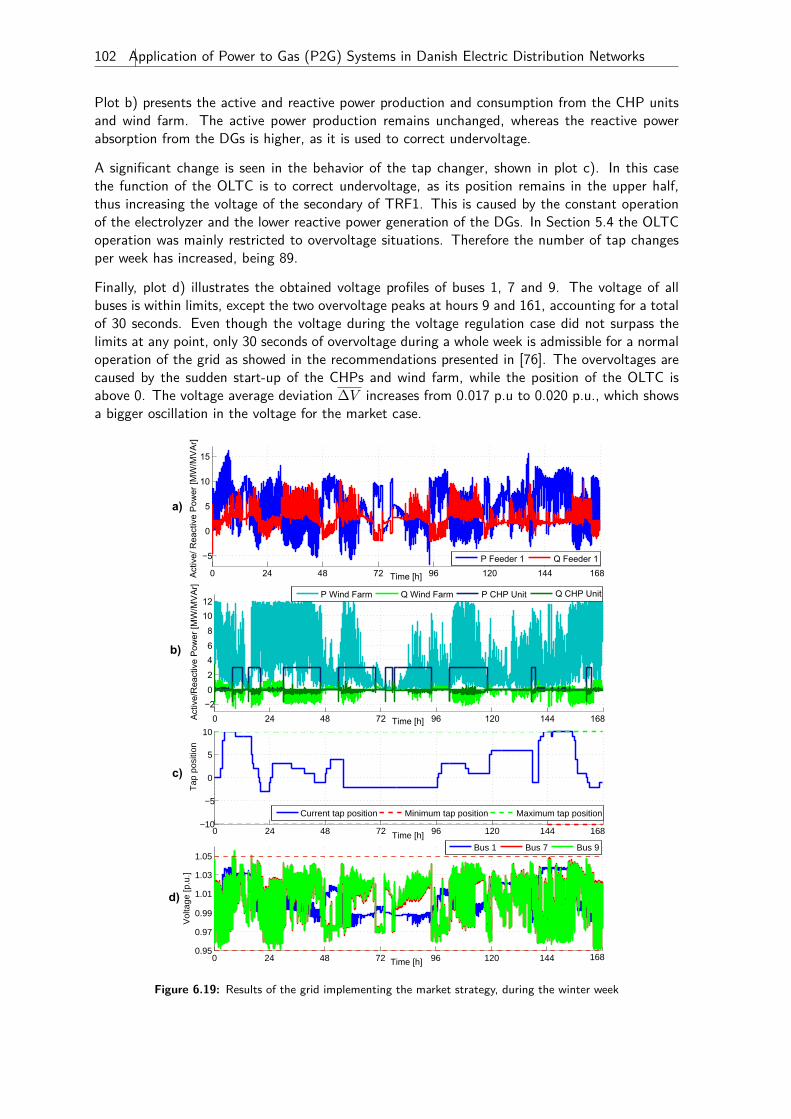
102 Application of Power to Gas (P2G) Systems in Danish Electric Distribution Networks
Plot b) presents the active and reactive power production and consumption from the CHP unitsand wind farm. The active power production remains unchanged, whereas the reactive powerabsorption from the DGs is higher, as it is used to correct undervoltage.
A significant change is seen in the behavior of the tap changer, shown in plot c). In this casethe function of the OLTC is to correct undervoltage, as its position remains in the upper half,thus increasing the voltage of the secondary of TRF1. This is caused by the constant operationof the electrolyzer and the lower reactive power generation of the DGs. In Section 5.4 the OLTCoperation was mainly restricted to overvoltage situations. Therefore the number of tap changesper week has increased, being 89.
Finally, plot d) illustrates the obtained voltage profiles of buses 1, 7 and 9. The voltage of allbuses is within limits, except the two overvoltage peaks at hours 9 and 161, accounting for a totalof 30 seconds. Even though the voltage during the voltage regulation case did not surpass thelimits at any point, only 30 seconds of overvoltage during a whole week is admissible for a normaloperation of the grid as showed in the recommendations presented in [76]. The overvoltages arecaused by the sudden start-up of the CHPs and wind farm, while the position of the OLTC isabove 0. The voltage average deviation ∆V increases from 0.017 p.u to 0.020 p.u., which showsa bigger oscillation in the voltage for the market case.
a)
c)
b)
d)
0 24 48 72 96 120 144 168
−5
0
5
10
15
Time [h]Activ
e/ R
eact
ive
Pow
er [M
W/M
VAr]
P Feeder 1 Q Feeder 1
0 24 48 72 96 120 144 168−202468
1012
Time [h]Activ
e/R
eact
ive
Pow
er [M
W/M
VAr]
Q CHP Unit P Wind Farm Q Wind Farm P CHP Unit Q CHP Unit
0 24 48 72 96 120 144 168
−5
0
5
10
Time [h]
Tap
pos
ition
−10
Current tap position Minimum tap position Maximum tap position
0 24 48 72 96 120 144 168
0.97
0.99
1.01
1.03
1.05
Time [h]
Vol
tage
[p.u
.]
0.95
Bus 1 Bus 7 Bus 9
Figure 6.19: Results of the grid implementing the market strategy, during the winter week
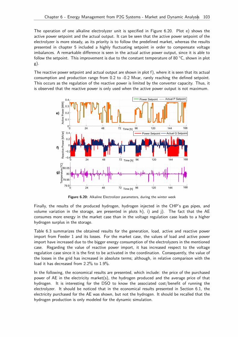
Chapter 6 - Energy Management from P2G Systems - Market and Dynamic Analysis 103
The operation of one alkaline electrolyzer unit is specified in Figure 6.20. Plot e) shows theactive power setpoint and the actual output. It can be seen that the active power setpoint of theelectrolyzer is more steady, as its priority is to follow the predefined market, whereas the resultspresented in chapter 5 included a highly fluctuating setpoint in order to compensate voltageimbalances. A remarkable difference is seen in the actual active power output, since it is able tofollow the setpoint. This improvement is due to the constant temperature of 80 °C, shown in plotg).
The reactive power setpoint and actual output are shown in plot f), where it is seen that its actualconsumption and production range from 0.2 to -0.2 Mvar, rarely reaching the defined setpoint.This occurs as the regulation of the reactive power is limited by the converter capacity. Thus, itis observed that the reactive power is only used when the active power output is not maximum.
e)
g)
f)
0 24 48 72 96 120 144 168
0.1
0.2
0.3
0.4
Time [h]
Activ
e Po
wer
[MW
]
0
Actual P Output Power Setpoint Actual P Setpoint
0 24 48 72 96 120 144 168
−0.2
0
0.2
0.4
Time [h]
Rea
ctiv
e Po
wer
[MVa
r]
−0.4
Actual Q Output Power Setpoint Actual Q Setpoint
0 24 48 72 96 120 144 16879.9
79.95
80
80.05
Time [h]
Tem
pera
ture
[ºC
]
Figure 6.20: Alkaline Electrolizer parameters, during the winter week
Finally, the results of the produced hydrogen, hydrogen injected in the CHP’s gas pipes, andvolume variation in the storage, are presented in plots h), i) and j). The fact that the AEconsumes more energy in the market case than in the voltage regulation case leads to a higherhydrogen surplus in the storage.
Table 6.3 summarizes the obtained results for the generation, load, active and reactive powerimport from Feeder 1 and its losses. For the market case, the values of load and active powerimport have increased due to the bigger energy consumption of the electrolyzers in the mentionedcase. Regarding the value of reactive power import, it has increased respect to the voltageregulation case since it is the first to be activated in the coordination. Consequently, the value ofthe losses in the grid has increased in absolute terms; although, in relative comparison with theload it has decreased from 2.2% to 1.9%.
In the following, the economical results are presented, which include: the price of the purchasedpower of AE in the electricity market(s), the hydrogen produced and the average price of thathydrogen. It is interesting for the DSO to know the associated cost/benefit of running theelectrolyzer. It should be noticed that in the economical results presented in Section 6.1, theelectricity purchased for the AE was shown, but not the hydrogen. It should be recalled that thehydrogen production is only modeled for the dynamic simulation.
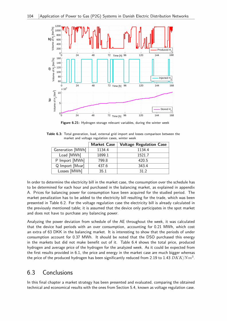
104 Application of Power to Gas (P2G) Systems in Danish Electric Distribution Networks
h)
i)
j)
0 24 48 72 96 120 144 168
200
400
600
800
1000
1200
Time [h]V
olum
e of
H2 [N
m3 /h
]0
Produced H2
0 24 48 72 96 120 144 168
60
80
100
120
140
160
Time [h]
Vol
ume
of H
2 [Nm
3 /h]
Injected H2
0 24 48 72 96 120 144 168
5
10
x 104
Time [h]
Vol
ume
of H
2 [Nm
3 ]
0
Stored H2
Market Case Voltage Regulation CaseGeneration [MWh] 1134.4 1134.4
Load [MWh] 1899.1 1521.7P Import [MWh] 799.8 420.5Q Import [Mvar] 437.6 343.4Losses [MWh] 35.1 31.2
In order to determine the electricity bill in the market case, the consumption over the schedule hasto be determined for each hour and purchased in the balancing market, as explained in appendixA. Prices for balancing power for consumption have been acquired for the studied period. Themarket penalization has to be added to the electricity bill resulting for the trade, which was beenpresented in Table 6.2. For the voltage regulation case the electricity bill is already calculated inthe previously mentioned table; it is assumed that the device only participates in the spot marketand does not have to purchase any balancing power.
Analyzing the power deviation from schedule of the AE throughout the week, it was calculatedthat the device had periods with an over consumption, accounting for 0.21 MWh, which costan extra of 63 DKK in the balancing market. It is interesting to show that the periods of underconsumption account for 0.37 MWh. It should be noted that the DSO purchased this energyin the markets but did not make benefit out of it. Table 6.4 shows the total price, producedhydrogen and average price of the hydrogen for the analyzed week. As it could be expected fromthe first results provided in 6.1, the price and energy in the market case are much bigger whereasthe price of the produced hydrogen has been significantly reduced from 2.19 to 1.43 DKK/Nm3.
6.3 ConclusionsIn this final chapter a market strategy has been presented and evaluated, comparing the obtainedtechnical and economical results with the ones from Section 5.4, known as voltage regulation case.
Table 6.3: Total generation, load, external grid import and losses comparison between themarket and voltage regulation cases, winter week
Figure 6.21: Hydrogen storage relevant variables, during the winter week
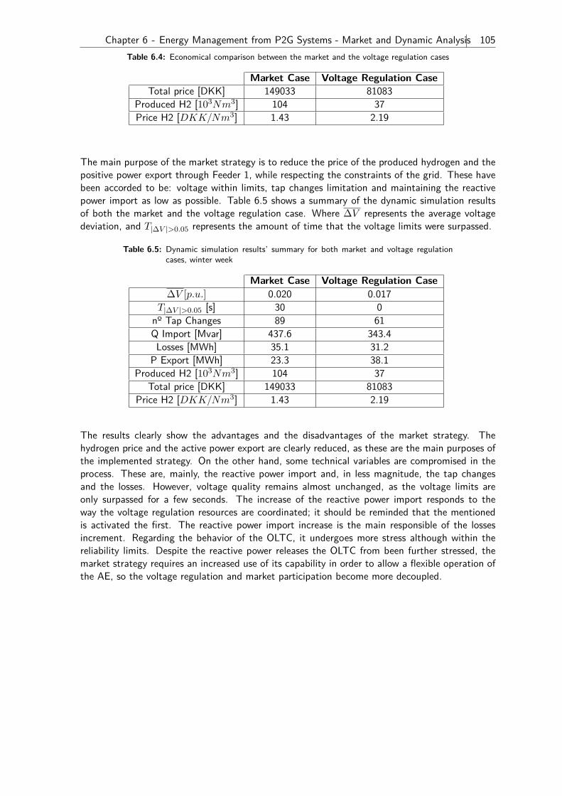
Chapter 6 - Energy Management from P2G Systems - Market and Dynamic Analysis 105Table 6.4: Economical comparison between the market and the voltage regulation cases
Market Case Voltage Regulation CaseTotal price [DKK] 149033 81083
Produced H2 [103Nm3] 104 37Price H2 [DKK/Nm3] 1.43 2.19
The main purpose of the market strategy is to reduce the price of the produced hydrogen and thepositive power export through Feeder 1, while respecting the constraints of the grid. These havebeen accorded to be: voltage within limits, tap changes limitation and maintaining the reactivepower import as low as possible. Table 6.5 shows a summary of the dynamic simulation resultsof both the market and the voltage regulation case. Where ∆V represents the average voltagedeviation, and T|∆V |>0.05 represents the amount of time that the voltage limits were surpassed.
Table 6.5: Dynamic simulation results’ summary for both market and voltage regulationcases, winter week
Market Case Voltage Regulation Case∆V [p.u.] 0.020 0.017
T|∆V |>0.05 [s] 30 0nº Tap Changes 89 61Q Import [Mvar] 437.6 343.4Losses [MWh] 35.1 31.2
P Export [MWh] 23.3 38.1Produced H2 [103Nm3] 104 37
Total price [DKK] 149033 81083Price H2 [DKK/Nm3] 1.43 2.19
The results clearly show the advantages and the disadvantages of the market strategy. Thehydrogen price and the active power export are clearly reduced, as these are the main purposes ofthe implemented strategy. On the other hand, some technical variables are compromised in theprocess. These are, mainly, the reactive power import and, in less magnitude, the tap changesand the losses. However, voltage quality remains almost unchanged, as the voltage limits areonly surpassed for a few seconds. The increase of the reactive power import responds to theway the voltage regulation resources are coordinated; it should be reminded that the mentionedis activated the first. The reactive power import increase is the main responsible of the lossesincrement. Regarding the behavior of the OLTC, it undergoes more stress although within thereliability limits. Despite the reactive power releases the OLTC from been further stressed, themarket strategy requires an increased use of its capability in order to allow a flexible operation ofthe AE, so the voltage regulation and market participation become more decoupled.

Chapter 7 - Conclusions and Future Work 107
7 Conclusions and Future Work7.1 ConclusionThe aim of this project was to analyze the capability of a Power to Gas system to provideenergy management and voltage regulation services to distribution grids with high wind powerpenetration. The focus has been placed on the arising issues that the Distribution System Operatormight encounter with the upcoming increase of renewable energy systems in medium voltagegrids. For this purpose, a benchmark 20 kV distribution grid was modeled and analyzed in theDIgSILENT PowerFactory simulation software. The grid consists of two feeders, which includeseveral buses with aggregated loads, a wind farm and a CHP plant. In addition to the electricaldistribution grid, simplifications of the district heating and gas networks are introduced in orderto evaluate their interactions with the electricity network. The district heating network representsthe aggregated heat demand that the CHP plant has to provide, whereas the gas grid representsa hydrogen storage and the natural gas flow towards the CHP. The hydrogen is assumed to beinjected to the CHP pipes with a volume limitation rate of 10%.
Firstly, the steady state behavior of the grid was analyzed taking into consideration two worstcases. These are (1): when the local generation, i.e. wind farm and CHP, are producing maximumpower output and the loads are at their minimum, and (2): when there is no local productionand the value of the demand is maximum. The results of the base case analysis, without anyvoltage regulation of grid assets, revealed that the most affected buses are 7 and 9 by overvoltageand undervoltage, respectively. It was found that the overvoltage in the first case surpassed theallowed voltage limits, determined by the grid codes. Further analysis in conducted with theapplication of an On-Load Tap Changer and reactive power compensation from the wind turbinesand CHPs, as they are commonly used by system operators. However, their regulating capacitywas not enough to rectify the high voltage deviation of the grid. Finally, the implementation ofelectrolyzers to bus 9 was assessed, as it is the most affected node regarding overvoltage. Thesize of the P2G system was determined to be the minimum in order to bring the voltage withinallowed limits. Thus, 15 alkaline electrolyzer modules, accounting for a load of 6.525 MW, wereimplemented to the OLTC scenario. The reactive power capability of the CHP and wind turbineswas not taken into account in the sizing. However, it was included in the coordination with theOLTC and electrolyzer, with the purpose of being activated during the dynamic simulations justbefore the voltage surpasses the allowed limits.
In order to incorporate the time-varying behavior of the assets in the grid, the dynamic modelsof its elements have been presented. As the CHP plant and the wind farm are assumed to beowned by private entities different from the DSO, they have been modeled as passive generators.Thus, the DSO can only regulate the power factor within the limits specified in the grid codes.More focus has been placed in those components where the DSO possesses full control for voltageregulation, i.e. OLTC and alkaline electrolyzer. Therefore, the most important implementationsare the active and reactive control of the alkaline electrolyzer, the Line Drop Compensationmodel of the OLTC and the power factor control of the CHP plant and wind turbines. Within themodels of the mentioned elements, decentralized voltage regulation coordination is implementedby adjusting the deadbands of the different voltage droops and OLTC controller. Furthermore,the heat and hydrogen production from both CHP and electrolyzer were modeled in order torepresent long-term dynamic models of the district heating and gas network respectively.
The dynamic behavior of the case study grid was analyzed by assessing the coordinated voltageregulation strategy of the previously mentioned elements. Regarding the voltage profile, the

108 Application of Power to Gas (P2G) Systems in Danish Electric Distribution Networks
obtained results corroborated the findings in the steady state analysis. The OLTC, both on itsown and together with the reactive power capability, is not able to bring the voltage withinadmissible limits. Furthermore, the excessive reactive power import when using the DG’s reactivepower capability leads to a significant increase of the grid losses. The voltage issues are correctedwith the implementation of the P2G system which, at the same time, reduces the grid lossesby almost 50% and demands negligible reactive power absorption for the DGs. Nevertheless,it was found that the regulating capacity of the alkaline electrolyzer was restricted by a lowoperating temperature which has resulted from stand-by periods. Furthermore, providing energymanagement services with the electrolyzer is not explicitly analyzed; the electrolyzer responds onlyto voltage signals and not to market prices. These issues are intended to be addressed by meansof implementing an intelligent market strategy for the P2G system. Regarding the hydrogen, itwas observed that the bleeding strategy cannot handle all the hydrogen that is produced duringthe process.
As the final contribution of this Master Thesis, a market strategy that copes with energy man-agement and voltage regulation has been developed. Additionally, it was intended to respect thetechnical constraints faced during the dynamic analysis of the case study, namely: voltage limits,daily tap changes below the maximum recommended bounds and reactive power absorption. Forthis purpose, an algorithm that estimates the different power absorption requirements of the elec-trolyzer has been developed. Additionally, a fuzzy logic decision system that determines the bidin the market has been implemented and new control models and voltage regulation coordinationhave been proposed. The results from the dynamic simulation showed an increased consumptionof the locally generated energy and a significant reduction in the cost of the produced energy, from2.19DKK/Nm3 to 1.43DKK/Nm3. These benefits have been obtained by providing flexibilityfrom the alkaline electrolyzer in the voltage regulation. However, the consequences are that thevoltage is closer to the limits, the reactive power absorption increases significantly and the gridlosses and tap changes present a slight increase. Nevertheless, the voltage remains within therecommended limits and the tap changes do not surpass the reliability constraint, which showsthe feasibility of the proposed market strategy and validates the economical improvement it canprovide. However, a cost benefit analysis has to be done to confirm the economical improvementof the presented strategy.
As the final conclusion of the present project, it can be stated that P2G is a very promisingtechnology that might have an important role in the future integrated Danish energy system,which is expected to interconnect in a flexible way the electrical, district heating and gas networksto integrate more wind power. The scope of this work has been focused on the electrical behaviorof the alkaline electrolyzer, which has been satisfactory tested to provide voltage regulation andenergy management services under electricity market conditions. For this purpose, its operationhas been coordinated with other typical voltage regulation elements of a distribution system,namely OLTC and reactive power. The findings of this project reveal that the DSO can decidethe price to pay for using the local generation to produce hydrogen, while maintaining the voltagewithin the admissible limits. This fact gains importance when placed in the context of the futureinterconnection of the three energy sectors, where the decision of transforming electricity togas/hydrogen will not only depend on the availability of the electricity but also on its price, whichare not always correlated. Nevertheless, in order to implement the technology in a profitable way,a cost/benefit analysis must be done. At present, there is a just a limited amount of ongoingP2G projects, since the technology is expensive and still in research status. With a reduction ofthe capital, maintenance and operation costs in the near future, a P2G operation strategy, as thepresented in this Master Thesis, could become economically feasible and open the possibility tonew business opportunities.
Chapter 7 - Conclusions and Future Work 109
7.2 Future WorkIn this final section, the relevant tasks that could be interesting to explore as future work arepresented.
• Operating the grid in meshed configuration: in the analyzed case study, the operation of theswitches was disregarded and the topology of the grid was permanently radial. Nevertheless,the DSO might close the switches in order to optimize the load flow or improve reliabilityunder contingency situations.
• Dynamic modeling of the wind turbines: their dynamic model, including the wind powercurve, rotor blade angle control and shaft, could be presented in order to increase theaccuracy of the active power generation.
• Grid state forecasting: in order to develop the market strategy, a load flow estimation wasapplied in order to represent the errors arising from a real forecast. Implementing a realgrid state forecast method would help to assess, in a more realistic way, the technical andeconomical impacts of implementing the proposed market strategy.
• Forward hourly direct signals to the OLTC with the desired tap position: in Section 6.2 aPI controller was proposed in order to keep the voltage according to an hourly set-point. Itwas observed that the voltage profile is kept almost perfectly at the set-point and the AEcould absorb the wind farm’s deviations from schedule. In order to achieve this, an hourlytap position signal has to be forwarded to the OLTC.
• Dynamic modeling of the district heating and gas networks: the dynamic simulations havebeen carried out without incorporating the possible delays associated to the water and gasflow dynamics, which might have lead to further operational constraints.
• Additional hydrogen consumption: the proposed hydrogen injection strategy was not ableto utilize all the production from the alkaline electrolyzers, hence, additional consumptionis required. Possible solutions for its use include: direct connection of the AE to thetransmission gas network, transforming the hydrogen into synthetic natural gas, includehydrogen mobility in the public transport of the area and including hydrogen-fired CHPplants.
• Intelligent temperature control method to allow complete disconnection of the electrolyzer:as shown in section 6.1, the electricity bill from participating in the electricity markets wouldbe further reduced if the lower power constraint is not respected. This method would requirepredicting the temperature of the device and timing the start-up, which can take up to 132minutes.


Appendices
111

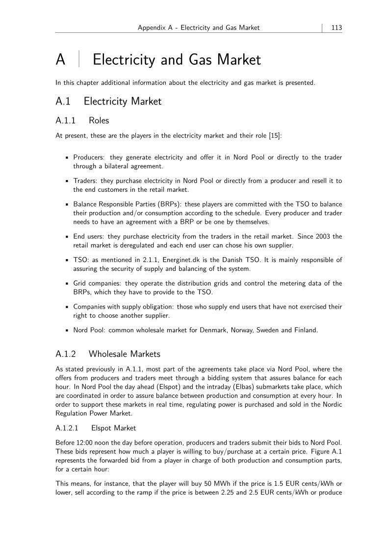
Appendix A - Electricity and Gas Market 113
A Electricity and Gas MarketIn this chapter additional information about the electricity and gas market is presented.
A.1 Electricity MarketA.1.1 RolesAt present, these are the players in the electricity market and their role [15]:
• Producers: they generate electricity and offer it in Nord Pool or directly to the traderthrough a bilateral agreement.
• Traders: they purchase electricity in Nord Pool or directly from a producer and resell it tothe end customers in the retail market.
• Balance Responsible Parties (BRPs): these players are committed with the TSO to balancetheir production and/or consumption according to the schedule. Every producer and traderneeds to have an agreement with a BRP or be one by themselves.
• End users: they purchase electricity from the traders in the retail market. Since 2003 theretail market is deregulated and each end user can chose his own supplier.
• TSO: as mentioned in 2.1.1, Energinet.dk is the Danish TSO. It is mainly responsible ofassuring the security of supply and balancing of the system.
• Grid companies: they operate the distribution grids and control the metering data of theBRPs, which they have to provide to the TSO.
• Companies with supply obligation: those who supply end users that have not exercised theirright to choose another supplier.
• Nord Pool: common wholesale market for Denmark, Norway, Sweden and Finland.
A.1.2 Wholesale MarketsAs stated previously in A.1.1, most part of the agreements take place via Nord Pool, where theoffers from producers and traders meet through a bidding system that assures balance for eachhour. In Nord Pool the day ahead (Elspot) and the intraday (Elbas) submarkets take place, whichare coordinated in order to assure balance between production and consumption at every hour. Inorder to support these markets in real time, regulating power is purchased and sold in the NordicRegulation Power Market.
A.1.2.1 Elspot Market
Before 12:00 noon the day before operation, producers and traders submit their bids to Nord Pool.These bids represent how much a player is willing to buy/purchase at a certain price. Figure A.1represents the forwarded bid from a player in charge of both production and consumption parts,for a certain hour:
This means, for instance, that the player will buy 50 MWh if the price is 1.5 EUR cents/kWh orlower, sell according to the ramp if the price is between 2.25 and 2.5 EUR cents/kWh or produce
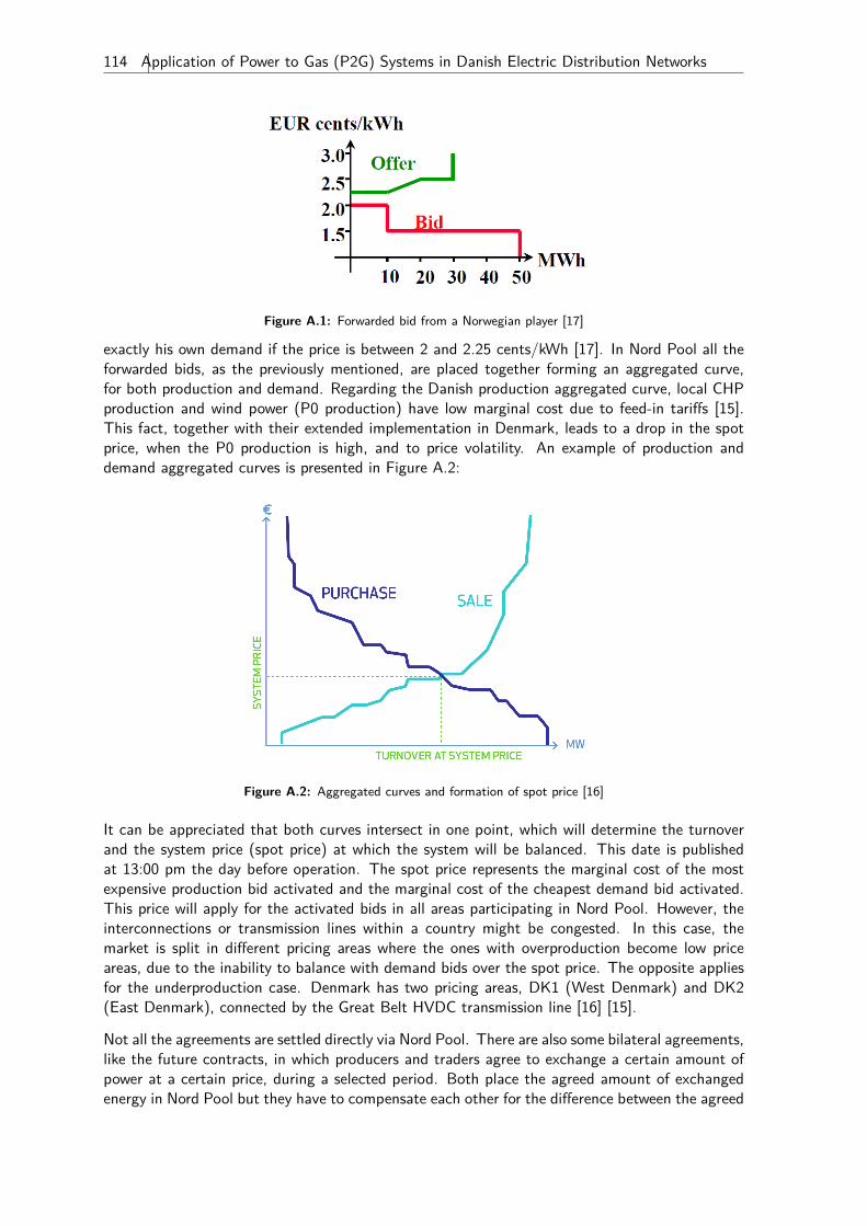
114 Application of Power to Gas (P2G) Systems in Danish Electric Distribution Networks
Figure A.1: Forwarded bid from a Norwegian player [17]
exactly his own demand if the price is between 2 and 2.25 cents/kWh [17]. In Nord Pool all theforwarded bids, as the previously mentioned, are placed together forming an aggregated curve,for both production and demand. Regarding the Danish production aggregated curve, local CHPproduction and wind power (P0 production) have low marginal cost due to feed-in tariffs [15].This fact, together with their extended implementation in Denmark, leads to a drop in the spotprice, when the P0 production is high, and to price volatility. An example of production anddemand aggregated curves is presented in Figure A.2:
Figure A.2: Aggregated curves and formation of spot price [16]
It can be appreciated that both curves intersect in one point, which will determine the turnoverand the system price (spot price) at which the system will be balanced. This date is publishedat 13:00 pm the day before operation. The spot price represents the marginal cost of the mostexpensive production bid activated and the marginal cost of the cheapest demand bid activated.This price will apply for the activated bids in all areas participating in Nord Pool. However, theinterconnections or transmission lines within a country might be congested. In this case, themarket is split in different pricing areas where the ones with overproduction become low priceareas, due to the inability to balance with demand bids over the spot price. The opposite appliesfor the underproduction case. Denmark has two pricing areas, DK1 (West Denmark) and DK2(East Denmark), connected by the Great Belt HVDC transmission line [16] [15].
Not all the agreements are settled directly via Nord Pool. There are also some bilateral agreements,like the future contracts, in which producers and traders agree to exchange a certain amount ofpower at a certain price, during a selected period. Both place the agreed amount of exchangedenergy in Nord Pool but they have to compensate each other for the difference between the agreed
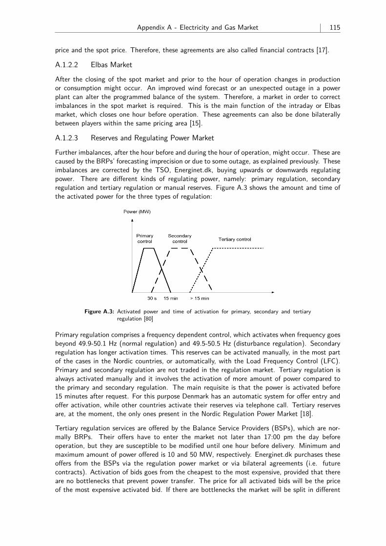
Appendix A - Electricity and Gas Market 115
price and the spot price. Therefore, these agreements are also called financial contracts [17].
A.1.2.2 Elbas Market
After the closing of the spot market and prior to the hour of operation changes in productionor consumption might occur. An improved wind forecast or an unexpected outage in a powerplant can alter the programmed balance of the system. Therefore, a market in order to correctimbalances in the spot market is required. This is the main function of the intraday or Elbasmarket, which closes one hour before operation. These agreements can also be done bilaterallybetween players within the same pricing area [15].
A.1.2.3 Reserves and Regulating Power Market
Further imbalances, after the hour before and during the hour of operation, might occur. These arecaused by the BRPs’ forecasting imprecision or due to some outage, as explained previously. Theseimbalances are corrected by the TSO, Energinet.dk, buying upwards or downwards regulatingpower. There are different kinds of regulating power, namely: primary regulation, secondaryregulation and tertiary regulation or manual reserves. Figure A.3 shows the amount and time ofthe activated power for the three types of regulation:
2.3. THE ENERGY MARKETS
Figure 2.7: Regulating power
The primary control is commonly referred to as frequency control. The ENTSO-E guidelines/agree-ments state that the frequency control should be activated if the frequency deviates from the pre-set50Hz by more than ±20mHz. The frequency control should be fully operational within 30 secondsof a deviation greater than 20mHz. The need for regulating power is rather limited in terms of theamount of power needed.
The secondary control (or Load Frequency Control) is utilized to support and relieve the primarycontrol. The secondary control reserves must be active no later than30 seconds after a deviation hasoccurred and the deviation in frequency must be within the limits no sooner than 15 minutes [13]after the regulation has begun.
The tertiary control covers the activation of manual reserves which are activated if the system unbal-ance is not restored for the hour of consumption.
The regulating power is an interesting topic when looking into flexible consumption and demandside management. The flexible units covered in this project, namely the EV and HP, are both capableof interacting with the balancing-market and assisting when in need for regulating power. The EVswill be able to directly and actively assist with both up- and down regulation of power, by consumingpower or delivering power back to the grid (V2G). The HPs will also be able to assist, but in a morepassive role than the EVs. The HPs will be able to stop consumption for some amount of time whenthere is a power deficiency as well as consuming when there is a surplus of energy in the grids.
Wind turbine production usually represents a low price in the markets since wind power productionis supported by taxes paid for by the end-consumers. As a fictitious example to illustrate the system,assume the following:
• The cost for producing 1 MWh by use of a traditional generator is 1€
• The cost for producing 1 MWh by use of a wind turbine is 2€
• The owner of the wind turbine receives a tax-support of 1.2€ per produced MWh
These simple statements reveal two interesting details. With the focus on green energy in Denmark, ithas become less lucrative to produce power by conventional methods since the competitive positionof the traditional generators has been artificially decreased. On the other hand it has become morelucrative to produce energy by green alternatives such as wind turbines due to the tax-support. The
15
Figure A.3: Activated power and time of activation for primary, secondary and tertiaryregulation [80]
Primary regulation comprises a frequency dependent control, which activates when frequency goesbeyond 49.9-50.1 Hz (normal regulation) and 49.5-50.5 Hz (disturbance regulation). Secondaryregulation has longer activation times. This reserves can be activated manually, in the most partof the cases in the Nordic countries, or automatically, with the Load Frequency Control (LFC).Primary and secondary regulation are not traded in the regulation market. Tertiary regulation isalways activated manually and it involves the activation of more amount of power compared tothe primary and secondary regulation. The main requisite is that the power is activated before15 minutes after request. For this purpose Denmark has an automatic system for offer entry andoffer activation, while other countries activate their reserves via telephone call. Tertiary reservesare, at the moment, the only ones present in the Nordic Regulation Power Market [18].
Tertiary regulation services are offered by the Balance Service Providers (BSPs), which are nor-mally BRPs. Their offers have to enter the market not later than 17:00 pm the day beforeoperation, but they are susceptible to be modified until one hour before delivery. Minimum andmaximum amount of power offered is 10 and 50 MW, respectively. Energinet.dk purchases theseoffers from the BSPs via the regulation power market or via bilateral agreements (i.e. futurecontracts). Activation of bids goes from the cheapest to the most expensive, provided that thereare no bottlenecks that prevent power transfer. The price for all activated bids will be the priceof the most expensive activated bid. If there are bottlenecks the market will be split in different
116 Application of Power to Gas (P2G) Systems in Danish Electric Distribution Networks
pricing areas, as in the case of the spot market. In order to ensure security of supply, Energinet.dkneeds to have available enough reserves for balancing the system in case of failure of the biggerproduction unit. For this purpose, it signs future contract with the BRPs. The reserve market iswhere the TSO and the BRPs meet for closing these kind of contracts [19].
As previously stated in A.1.1, imbalances are produced by the BRPs. This means that their actualproduction or consumption, measured during the hour of operation, differs from the schedule.Therefore, if they have a negative imbalance this energy has to be bought from the Energinet.dk.If the imbalance is positive Energinet.dk will buy the surplus. This energy is bough in the so calledbalancing market and it is closely related to the regulation power market. Whereas the regulatingpower is used in order to correct the systems’ imbalance the balancing power is purchased orsold in order to correct the BRPs’ individual imbalance. The price to pay by the BRPs for thebalancing power depends on the direction of the system’s imbalance: if the system has a surplus,the BRPs that incur in a negative imbalance (correcting the system’s surplus) buy this energy atspot price. If they have a surplus (further increasing the system’s imbalance) Energinet.dk buysthis energy at the upwards regulating power price. The opposite applies in case of a power deficitin the system. P0 producers are exempt to pay for balancing power. Through the PSO tariffEnerginet.dk covers the cost of the P0 producers’ imbalances, as well as the feed-in tariffs thatapply for them as explained in A.1.2.1 [19] [18].
A.2 Gas MarketThe Danish gas market is liberalized since 2004, which means that every customer is free tochoose its supplier. Nowadays there are three available capacity trading facilities [81]:
A.2.1 GasPoint NordicGasPoint Nordic is the wholesale market of natural gas. It was previously known as NordPoolGas, however, since 2012 it is owned by Energinet.dk and thus the name was changed. Thegas exchange is offered in several time ranges: for the next day, the next month, within a day,within a weekend, within a month and finally physical delivery in Denmark and Germany. It is ananonymous and real-time electronic system where traders can place purchase and bids on salesall the time.
A.2.2 Gas Transfer Facility (GTF)GTF is a virtual trading facility operated by Energinet.dk. It enables intra-day gas trading amongshippers before and during a day. GTF is only the mean of communication between the shippersand it is a free service.
A.2.3 PRISMAPRISMA is the facility that enables trading gas capacity across European borders. The shipperscan participate in four different auctions: day-ahead, per month, per quarter of a year or per year.There are three entry-exit points in Denmark: Nybro, the entry point of the gas from the NorthSea; Ellund, in the border with Germany; and Dragør, in the border with Sweden.
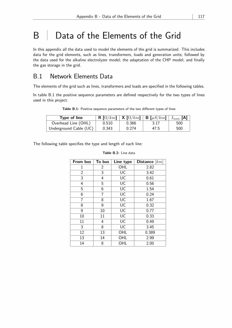
Appendix B - Data of the Elements of the Grid 117
B Data of the Elements of the GridIn this appendix all the data used to model the elements of the grid is summarized. This includesdata for the grid elements, such as lines, transformers, loads and generation units; followed bythe data used for the alkaline electrolyzer model; the adaptation of the CHP model; and finallythe gas storage in the grid.
B.1 Network Elements DataThe elements of the grid such as lines, transformers and loads are specified in the following tables.
In table B.1 the positive sequence parameters are defined respectively for the two types of linesused in this project.
Table B.1: Positive sequence parameters of the two different types of lines
Type of line R [Ω/km] X [Ω/km] B [µS/km] Inom [A]Overhead Line (OHL) 0.510 0.366 3.17 500
Underground Cable (UC) 0.343 0.274 47.5 500
The following table specifies the type and length of each line:
Table B.2: Line data
From bus To bus Line type Distance [km]1 2 OHL 2.822 3 UC 3.423 4 UC 0.614 5 UC 0.565 6 UC 1.546 7 UC 0.247 8 UC 1.678 9 UC 0.329 10 UC 0.7710 11 UC 0.3311 4 UC 0.493 8 UC 3.4512 13 OHL 0.38913 14 OHL 2.9914 8 OHL 2.00
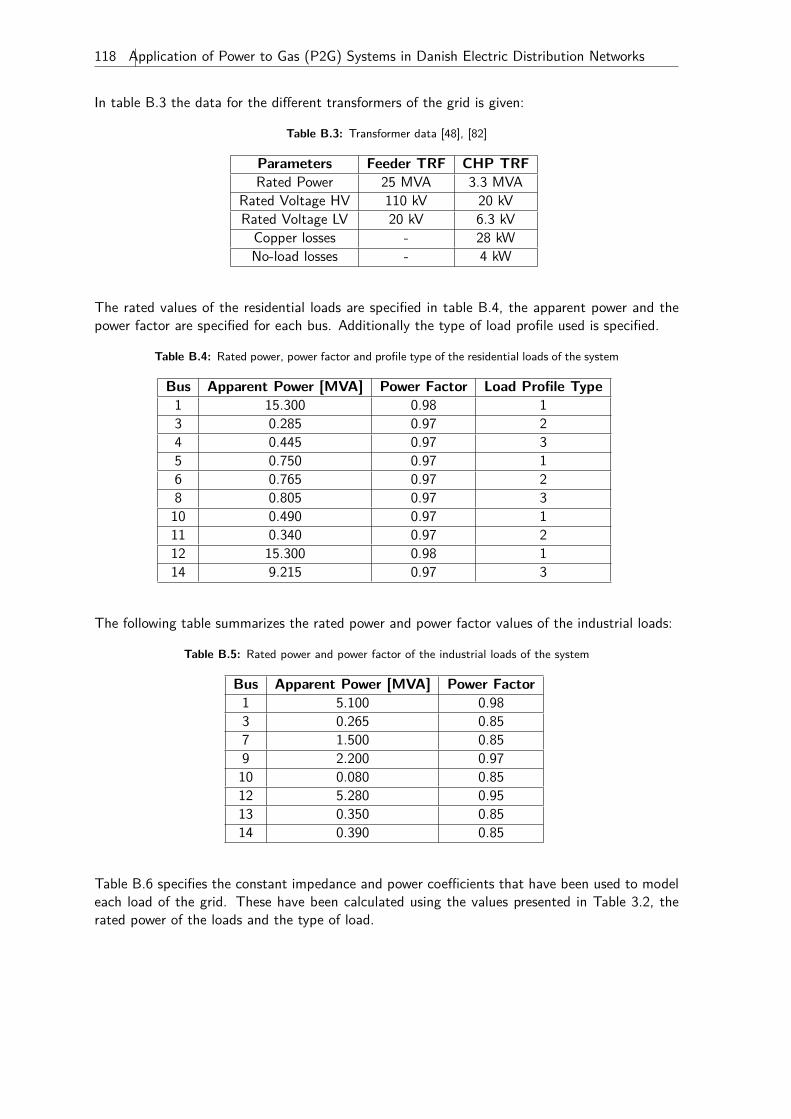
118 Application of Power to Gas (P2G) Systems in Danish Electric Distribution Networks
In table B.3 the data for the different transformers of the grid is given:
Table B.3: Transformer data [48], [82]
Parameters Feeder TRF CHP TRFRated Power 25 MVA 3.3 MVA
Rated Voltage HV 110 kV 20 kVRated Voltage LV 20 kV 6.3 kVCopper losses - 28 kWNo-load losses - 4 kW
The rated values of the residential loads are specified in table B.4, the apparent power and thepower factor are specified for each bus. Additionally the type of load profile used is specified.
Table B.4: Rated power, power factor and profile type of the residential loads of the system
Bus Apparent Power [MVA] Power Factor Load Profile Type1 15.300 0.98 13 0.285 0.97 24 0.445 0.97 35 0.750 0.97 16 0.765 0.97 28 0.805 0.97 310 0.490 0.97 111 0.340 0.97 212 15.300 0.98 114 9.215 0.97 3
The following table summarizes the rated power and power factor values of the industrial loads:
Table B.5: Rated power and power factor of the industrial loads of the system
Bus Apparent Power [MVA] Power Factor1 5.100 0.983 0.265 0.857 1.500 0.859 2.200 0.9710 0.080 0.8512 5.280 0.9513 0.350 0.8514 0.390 0.85
Table B.6 specifies the constant impedance and power coefficients that have been used to modeleach load of the grid. These have been calculated using the values presented in Table 3.2, therated power of the loads and the type of load.
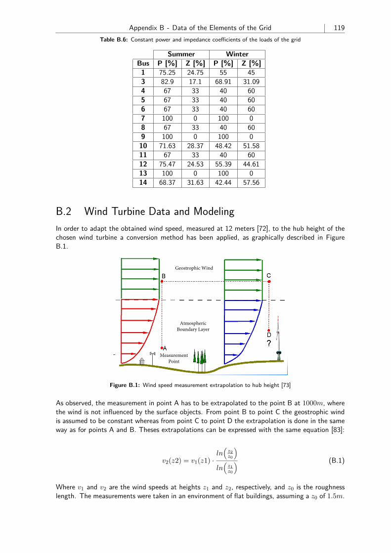
Appendix B - Data of the Elements of the Grid 119Table B.6: Constant power and impedance coefficients of the loads of the grid
Summer WinterBus P [%] Z [%] P [%] Z [%]1 75.25 24.75 55 453 82.9 17.1 68.91 31.094 67 33 40 605 67 33 40 606 67 33 40 607 100 0 100 08 67 33 40 609 100 0 100 010 71.63 28.37 48.42 51.5811 67 33 40 6012 75.47 24.53 55.39 44.6113 100 0 100 014 68.37 31.63 42.44 57.56
B.2 Wind Turbine Data and ModelingIn order to adapt the obtained wind speed, measured at 12 meters [72], to the hub height of thechosen wind turbine a conversion method has been applied, as graphically described in FigureB.1.
Universität Stuttgart
Vorl. Windenergienutzung I (SS 2011 ) - Der Wind 2.15
U
Europäischer Wind Atlas: Methodik
Methode für die horizontale und vertikale Extrapolation vonmeteorologischen Daten und Abschätzung der WindressourcenHauptannahme: - Geostrophischer Wind ist über große Entfernungen konstant
Transformation einer Windgeschwindigkeit am Punkt A an einen beliebigen Punkt D
• Wind am Punkt A wird von allen Einflüssen durch Orographie, Rauhigkeitenund Hindernissen bereinigt
• geostrophischer Wind (B,C)
• Einfügen lokaler Ereignisse am Punkt D
Geostrophic Wind
AtmosphericBoundary Layer
Measurement Point
Figure B.1: Wind speed measurement extrapolation to hub height [73]
As observed, the measurement in point A has to be extrapolated to the point B at 1000m, wherethe wind is not influenced by the surface objects. From point B to point C the geostrophic windis assumed to be constant whereas from point C to point D the extrapolation is done in the sameway as for points A and B. Theses extrapolations can be expressed with the same equation [83]:
v2(z2) = v1(z1) ·ln(z2z0
)ln(z1z0
) (B.1)
Where v1 and v2 are the wind speeds at heights z1 and z2, respectively, and z0 is the roughnesslength. The measurements were taken in an environment of flat buildings, assuming a z0 of 1.5m.
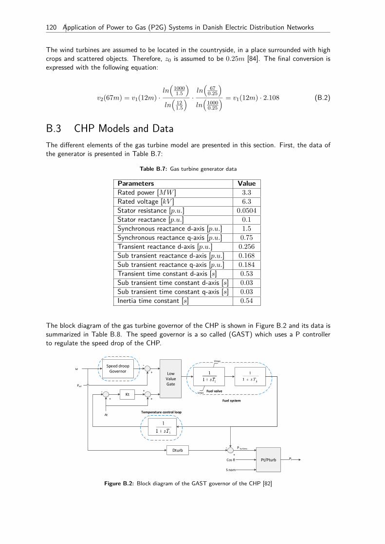
120 Application of Power to Gas (P2G) Systems in Danish Electric Distribution Networks
The wind turbines are assumed to be located in the countryside, in a place surrounded with highcrops and scattered objects. Therefore, z0 is assumed to be 0.25m [84]. The final conversion isexpressed with the following equation:
v2(67m) = v1(12m) ·ln(
10001.5
)ln(
121.5
) · ln(
670.25
)ln(
10000.25
) = v1(12m) · 2.108 (B.2)
B.3 CHP Models and DataThe different elements of the gas turbine model are presented in this section. First, the data ofthe generator is presented in Table B.7:
Table B.7: Gas turbine generator data
Parameters ValueRated power [MW ] 3.3Rated voltage [kV ] 6.3Stator resistance [p.u.] 0.0504Stator reactance [p.u.] 0.1Synchronous reactance d-axis [p.u.] 1.5Synchronous reactance q-axis [p.u.] 0.75Transient reactance d-axis [p.u.] 0.256Sub transient reactance d-axis [p.u.] 0.168Sub transient reactance q-axis [p.u.] 0.184Transient time constant d-axis [s] 0.53Sub transient time constant d-axis [s] 0.03Sub transient time constant q-axis [s] 0.03Inertia time constant [s] 0.54
The block diagram of the gas turbine governor of the CHP is shown in Figure B.2 and its data issummarized in Table B.8. The speed governor is a so called (GAST) which uses a P controllerto regulate the speed drop of the CHP.
Speed droopGovernor
LowValueGate
Dturb
ω
Kt
Pref
P turbine
At
Vmin
Vmax
Fuel valve
Temperature control loop
+
+
+
-
-
+
-
+Fuel system
Pt/PturbCos θ
S nom
Pt
Figure B.2: Block diagram of the GAST governor of the CHP [82]
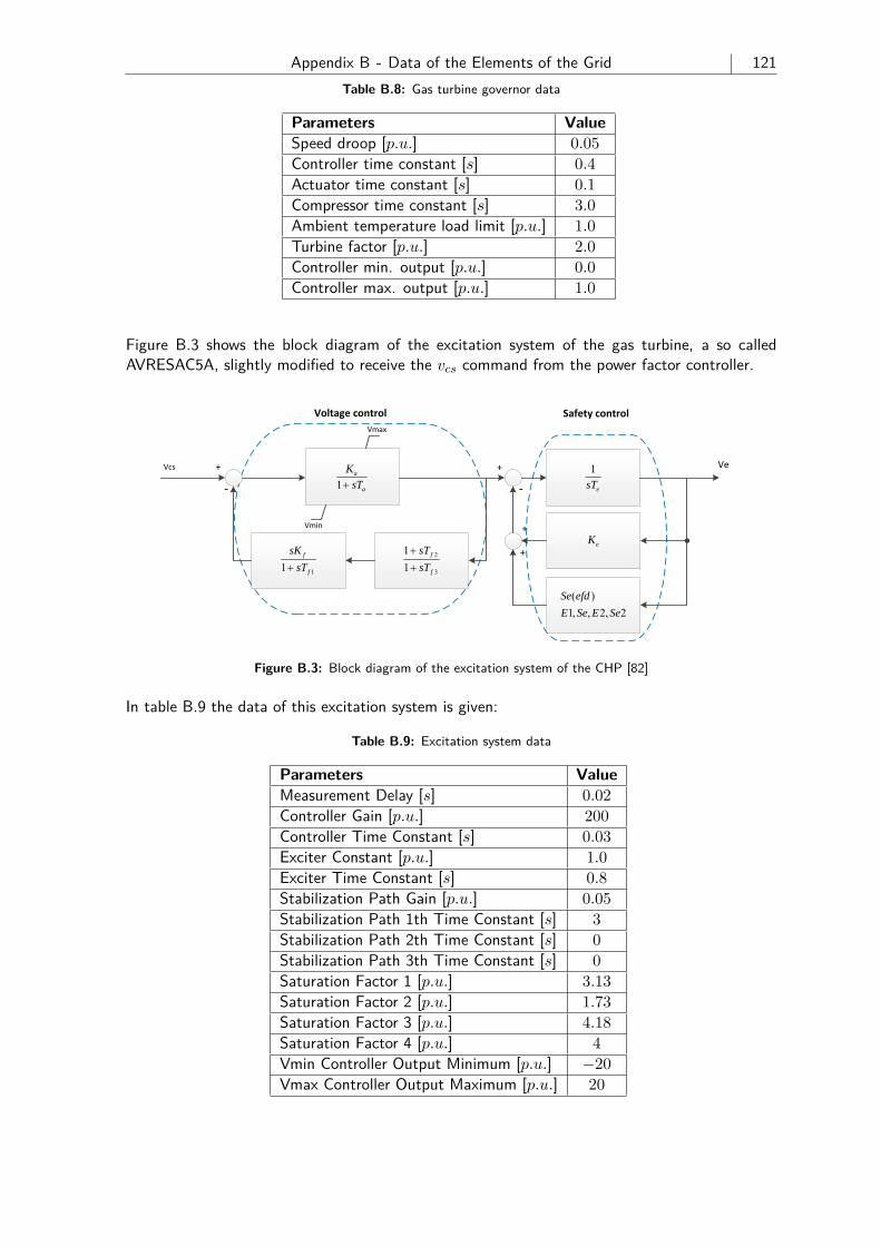
Appendix B - Data of the Elements of the Grid 121Table B.8: Gas turbine governor data
Parameters ValueSpeed droop [p.u.] 0.05Controller time constant [s] 0.4Actuator time constant [s] 0.1Compressor time constant [s] 3.0Ambient temperature load limit [p.u.] 1.0Turbine factor [p.u.] 2.0Controller min. output [p.u.] 0.0Controller max. output [p.u.] 1.0
Figure B.3 shows the block diagram of the excitation system of the gas turbine, a so calledAVRESAC5A, slightly modified to receive the vcs command from the power factor controller.
Ve
1a
a
KsT
11f
f
sKsT
2
3
11
f
f
sTsT
1
esT
eK
( )1, , 2, 2
Se efdE Se E Se
Vmax
Vmin
‐ ‐
+
+
+
+
Voltage control Safety control
Vcs
Figure B.3: Block diagram of the excitation system of the CHP [82]
In table B.9 the data of this excitation system is given:
Table B.9: Excitation system data
Parameters ValueMeasurement Delay [s] 0.02Controller Gain [p.u.] 200Controller Time Constant [s] 0.03Exciter Constant [p.u.] 1.0Exciter Time Constant [s] 0.8Stabilization Path Gain [p.u.] 0.05Stabilization Path 1th Time Constant [s] 3Stabilization Path 2th Time Constant [s] 0Stabilization Path 3th Time Constant [s] 0Saturation Factor 1 [p.u.] 3.13Saturation Factor 2 [p.u.] 1.73Saturation Factor 3 [p.u.] 4.18Saturation Factor 4 [p.u.] 4Vmin Controller Output Minimum [p.u.] −20Vmax Controller Output Maximum [p.u.] 20
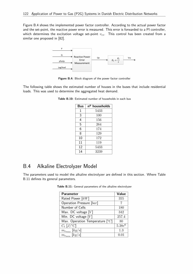
122 Application of Power to Gas (P2G) Systems in Danish Electric Distribution Networks
Figure B.4 shows the implemented power factor controller. According to the actual power factorand the set-point, the reactive power error is measured. This error is forwarded to a PI controller,which determines the excitation voltage set-point vcs. This control has been created from asimilar one proposed in [82].
Reactive Power Error
Measurement
P
Q
pfsetp
Lag/lead
Qe Vcs
Figure B.4: Block diagram of the power factor controller
The following table shows the estimated number of houses in the buses that include residentialloads. This was used to determine the aggregated heat demand.
Table B.10: Estimated number of households in each bus
Bus nº households1 54333 1004 1565 2646 1748 12910 17211 11912 543314 3239
B.4 Alkaline Electrolyzer ModelThe parameters used to model the alkaline electrolyzer are defined in this section. Where TableB.11 defines its general parameters.
Table B.11: General parameters of the alkaline electrolyzer
Parameter ValueRated Power [kW ] 355Operation Pressure [bar] 7Number of Cells 180Max. DC voltage [V ] 342Min. DC voltage [V ] 257.4Max. Operation Temperature [°C] 80Ct [J/°C] 5.38e6
memax [kg/s] 1.3memin [kg/s] 0.01
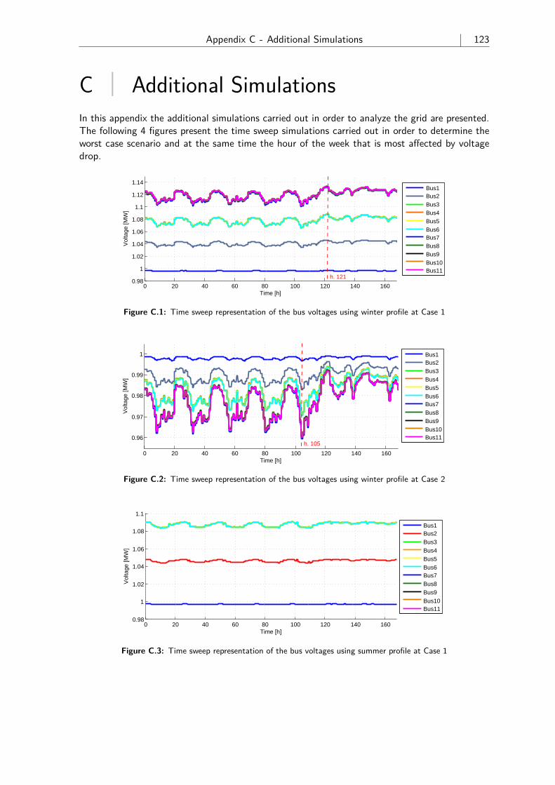
Appendix C - Additional Simulations 123
C Additional SimulationsIn this appendix the additional simulations carried out in order to analyze the grid are presented.The following 4 figures present the time sweep simulations carried out in order to determine theworst case scenario and at the same time the hour of the week that is most affected by voltagedrop.
0 20 40 60 80 100 120 140 1600.98
1
1.02
1.04
1.06
1.08
1.1
1.12
1.14
Time [h]
Vol
tage
[MW
]
Bus1Bus2Bus3Bus4Bus5Bus6Bus7Bus8Bus9Bus10Bus11
h. 121
Figure C.1: Time sweep representation of the bus voltages using winter profile at Case 1
0 20 40 60 80 100 120 140 160
0.96
0.97
0.98
0.99
1
Time [h]
Vol
tage
[MW
]
Bus1Bus2Bus3Bus4Bus5Bus6Bus7Bus8Bus9Bus10Bus11
h. 105
Figure C.2: Time sweep representation of the bus voltages using winter profile at Case 2
0 20 40 60 80 100 120 140 1600.98
1
1.02
1.04
1.06
1.08
1.1
Time [h]
Vol
tage
[MW
]
Bus1Bus2Bus3Bus4Bus5Bus6Bus7Bus8Bus9Bus10Bus11
Figure C.3: Time sweep representation of the bus voltages using summer profile at Case 1
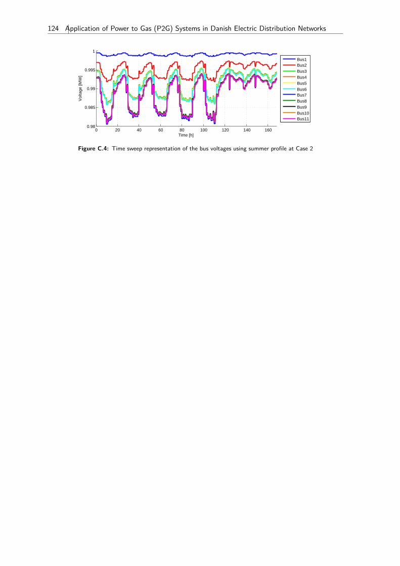
124 Application of Power to Gas (P2G) Systems in Danish Electric Distribution Networks
0 20 40 60 80 100 120 140 1600.98
0.985
0.99
0.995
1
Time [h]
Vol
tage
[MW
]
Bus1Bus2Bus3Bus4Bus5Bus6Bus7Bus8Bus9Bus10Bus11
Figure C.4: Time sweep representation of the bus voltages using summer profile at Case 2
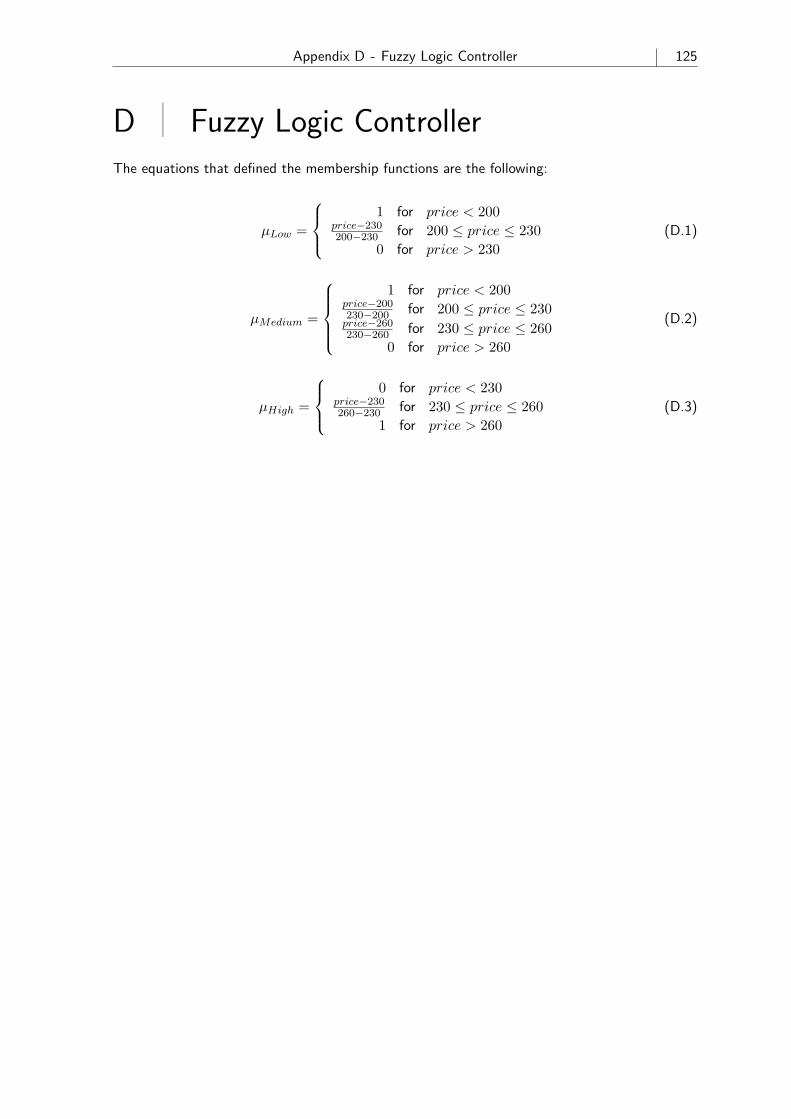
Appendix D - Fuzzy Logic Controller 125
D Fuzzy Logic ControllerThe equations that defined the membership functions are the following:
µLow =
1 for price < 200
price−230200−230 for 200 ≤ price ≤ 230
0 for price > 230(D.1)
µMedium =
1 for price < 200
price−200230−200 for 200 ≤ price ≤ 230price−260230−260 for 230 ≤ price ≤ 260
0 for price > 260
(D.2)
µHigh =
0 for price < 230
price−230260−230 for 230 ≤ price ≤ 260
1 for price > 260(D.3)

Bibliography 127
Bibliography[1] Danish Government, “Energy strategy 2050,” www.ens.dk, 2011, accessed 02-10-2014.
[2] Danish Ministry of Climate, Energy and Building, “Smart grid strategy - the intelligentenergy system of the future,” www.kemin.dk, 2013, accessed 02-10-2014.
[3] M. Brower, “Wind energy forecasting,” www.awstruepower.com, 2011, accessed02-10-2014.
[4] HyUnder, “Assessment of the potential, the actors and relevant business cases for largescale and long term storage of renewable electricity by hydrogen underground storage ineurope,” http://www.hyunder.eu/, 2013, accessed 02-10-2014.
[5] E. EASE, “Joint ease/eera recommendations for a european energy storage technologydevelopment roadmap towards 2030,” http://www.ease-storage.eu/, 2013, accessed02-10-2014.
[6] C. Baumann, R. Schuster, and A. Moser, “Economic potential of power-to-gas energystorages,” in European Energy Market (EEM), 2013 10th International Conference on the,May 2013, pp. 1–6.
[7] M. Korpas and T. Gjengedal, “Opportunities for hydrogen storage in connection withstochastic distributed generation,” in Probabilistic Methods Applied to Power Systems,2006. PMAPS 2006. International Conference on, June 2006, pp. 1–8.
[8] Øystein Ulleberg, T. Nakken, and A. Eté, “The wind/hydrogen demonstration system atutsira in norway: Evaluation of system performance using operational data and updatedhydrogen energy system modeling tools,” International Journal of Hydrogen Energy,vol. 35, no. 5, pp. 1841 – 1852, 2010. [Online]. Available:http://www.sciencedirect.com/science/article/pii/S0360319909016759
[9] L. Ramirez-Elizondo, G. Paap, and N. Woudstra, “The application of a fuel cell-electrolyzerarrangement as a power balancing set-up in autonomous renewable energy systems,” inPower Symposium, 2008. NAPS ’08. 40th North American, Sept 2008, pp. 1–8.
[10] M. Little, M. Thomson, and D. Infield, “Electrical integration of renewable energy intostand-alone power supplies incorporating hydrogen storage,” International Journal ofHydrogen Energy, vol. 32, no. 10–11, pp. 1582 – 1588, 2007, EHEC2005. [Online].Available: http://www.sciencedirect.com/science/article/pii/S0360319906005209
[11] H. K. Jacobsen and S. T. Schröder, “Curtailment of renewable generation: Economicoptimality and incentives,” Energy Policy, vol. 49, no. 0, pp. 663 – 675, 2012, specialSection: Fuel Poverty Comes of Age: Commemorating 21 Years of Research and Policy.[Online]. Available: http://www.sciencedirect.com/science/article/pii/S030142151200585X
[12] T. Zhou, D. Lu, H. Fakham, and B. Francois, “Power flow control in different time scalesfor a wind/hydrogen/super-capacitors based active hybrid power system,” in PowerElectronics and Motion Control Conference, 2008. EPE-PEMC 2008. 13th, Sept 2008, pp.2205–2210.
128 Application of Power to Gas (P2G) Systems in Danish Electric Distribution Networks
[13] Energinet.dk, “Danish transmission system ultimo 2014,”http://energinet.dk/EN/ANLAEG-OG-PROJEKTER/Generelt-om-elanlaeg/Sider/default.aspx, 2014, accessed14-10-2014.
[14] Nordic Energy Regulators, “Economic regulation of electricity grids in nordic countries,”http://www.nordicenergyregulators.org/wp-content/uploads/2013/02/Economic_regulation_of_electricity_grids_in_Nordic_countries.pdf,2011, accessed 15-10-2014.
[15] Energinet.dk, “Regulation a: Principles of the electricity market,”http://www.energinet.dk, 2007, accessed 17-10-2014.
[16] Nord Pool, “Day-ahead market - elspot,” http://www.nordpoolspot.com, 2014, accessed17-10-2014.
[17] A. P. Houmøller, “The nordic power exchange nord pool and the nordic model for aliberalised power market,” http://www.nordpoolspot.com, 2003, accessed 17-10-2014.
[18] Nordic Energy Regulators, “Harmonising the balancing market,”http://www.nordicenergyregulators.org, 2010, accessed 17-10-2014.
[19] Energinet.dk, “Regulation c2: The balancing market and balance settlement,”http://www.energinet.dk, 2008, accessed 17-10-2014.
[20] D. E. A. Energinet.dk, “Smart grid in denmark 2.0,” http://www.energinet.dk, 2012,accessed 17-10-2014.
[21] D. Dansk Energi, “District heating - danish and chinese experiences,”http://dbdh.dk/publications/, 2013.
[22] Danish Energy Agency, “Energy statistics 2012,” http://www.ens.dk, 2014, accessed19-10-2014.
[23] U.S. Environmental Protection Agency, “Catalog of chp technologies,”http://www.epa.gov/chp/documents/catalog_chptech_full.pdf, 2014, accessed19-10-2014.
[24] Danish Energy Agency, “Energy statistics 2013,” http://www.ens.dk, 2014, accessed09-01-2015.
[25] C. S.-M. S. N. S. Hans F. Ravn, Jannik Riisom, “Modelling danish local chp on marketconditions,” http://orbit.dtu.dk/en, 2004, accessed 19-10-2014.
[26] 2G CENERGY®, “2g cenergy®monthly newsletter,”http://www.2g-cenergy.com/pdfs/2G-CENERGY-News-Letter-June-2013.pdf, 2013,accessed 19-10-2014.
[27] Danish Energy Agency, “Oil and gas production in denmark 2013,”http://www.ens.dk/sites/ens.dk/files/energistyrelsen/Nyheder/2014/oil_and_gas_production_in_denmark_2013_uk.pdf,2014, accessed 16-10-2014.
[28] Energinet.dk, “Shipping gas in denmark,”http://www.energinet.dk/SiteCollectionDocuments/Engelske2008, accessed 16-10-2014.
Bibliography 129
[29] ——, “Structure of the natural gas system,” http://energinet.dk/EN/ANLAEG-OG-PROJEKTER/Generelt-om-gasanlaeg/Sider/Naturgassystemets-opbygning.aspx, 2013,accessed 16-10-2014.
[30] ——, “Illustration of the gas system in denmark,”http://energinet.dk/Flash/Forside/UK/index.html?target=gas_net, 2014, accessed16-10-2014.
[31] Energi Styrelsen, “Gas storage in denmark,” http://www.ens.dk/node/1971, 2008,accessed 17-10-2014.
[32] A. Ursua, L. Gandia, and P. Sanchis, “Hydrogen production from water electrolysis: Currentstatus and future trends,” Proceedings of the IEEE, vol. 100, no. 2, pp. 410–426, Feb 2012.
[33] M. Bodner, A. Hofer, and V. Hacker, “H2 generation from alkaline electrolyzer,” WileyInterdisciplinary Reviews: Energy and Environment, 2014.
[34] Øystein Ulleberg, “Modeling of advanced alkaline electrolyzers: a system simulationapproach,” International Journal of Hydrogen Energy, vol. 28, no. 1, pp. 21 – 33, 2003.[Online]. Available: http://www.sciencedirect.com/science/article/pii/S0360319902000332
[35] F. Barbir, “Pem electrolysis for production of hydrogen from renewable energy sources,”Solar Energy, vol. 78, no. 5, pp. 661 – 669, 2005, solar Hydrogen. [Online]. Available:http://www.sciencedirect.com/science/article/pii/S0038092X04002464
[36] H. Görgün, “Dynamic modelling of a proton exchange membrane (pem) electrolyzer,”International Journal of Hydrogen Energy, vol. 31, no. 1, pp. 29 – 38, 2006. [Online].Available: http://www.sciencedirect.com/science/article/pii/S0360319905000868
[37] M. Ni, M. K. Leung, and D. Y. Leung, “Technological development of hydrogen productionby solid oxide electrolyzer cell (soec),” International Journal of Hydrogen Energy, vol. 33,no. 9, pp. 2337 – 2354, 2008. [Online]. Available:http://www.sciencedirect.com/science/article/pii/S0360319908002255
[38] M. Zahid, J. Schefold, and A. Brisse, “High-temperature water electrolysis using planarsolid oxide fuel cell technology: a review,” Hydrogen and Fuel Cells, Fundamentals,Technologies and Applications, Wiley-VCH, Weinheim, pp. 227–242, 2010.
[39] S. Studer, S. Stucki, and J. D. Speight, Hydrogen as a Fuel. Wiley-VCH Verlag GmbH &Co. KGaA, 2008. [Online]. Available: http://dx.doi.org/10.1002/9783527622894.ch3
[40] D. Haeseldonckx and W. D’haeseleer, “The use of the natural-gas pipeline infrastructurefor hydrogen transport in a changing market structure,” International Journal of HydrogenEnergy, vol. 32, no. 10–11, pp. 1381 – 1386, 2007, EHEC2005. [Online]. Available:http://www.sciencedirect.com/science/article/pii/S0360319906004940
[41] K. Altfeld and D. Pinchbeck, “Admissible hydrogen concentrations in natural gas systems,”www.gas-for-energy.com, 2013, accessed 02-03-2015.
[42] A. Godula-Jopek, Hydrogen Production: by Electrolysis. Wiley-VCH, 2015.
[43] BioCat, “Biocat project - power to gas via biological catalysis,” http://biocat-project.com,2012, accessed 20-10-2014.
[44] “Denmark turns excess wind power into gas via hydrogenics tech,” Fuel Cells Bulletin, vol.2014, no. 3, pp. 8 – 9, 2014. [Online]. Available:http://www.sciencedirect.com/science/article/pii/S1464285914700823
130 Application of Power to Gas (P2G) Systems in Danish Electric Distribution Networks
[45] “Largest power-to-gas facility now operating with hydrogenics tech,” Fuel Cells Bulletin,vol. 2013, no. 7, pp. 9 –, 2013. [Online]. Available:http://www.sciencedirect.com/science/article/pii/S1464285913702645
[46] E. P. Mainz, “Energie park mainz,” http://energiepark-mainz.de/, 2015, accessed10-05-2015.
[47] I. de Cerio Mendaza, B. Bak-Jensen, and Z. Chen, “Alkaline electrolyzer and v2g systemdigsilent models for demand response analysis in future distribution networks,” pp. 1–8,June 2013.
[48] K. Rudion, A. Orths, Z. Styczynski, and K. Strunz, “Design of benchmark of mediumvoltage distribution network for investigation of dg integration,” in Power EngineeringSociety General Meeting, 2006. IEEE, 2006, pp. 6 pp.–.
[49] T. A. Short, Electric Power Distribution Handbook. CRC Press, 2014.
[50] H. L. Willis, Electrical Transmission and Distribution Reference Book. Raleigh, 1997.
[51] X. Guo, J. Du, and C. Qi, “Study and application of switching operation of 10kv lines ringnetwork in urban power distribution network,” in Electricity Distribution (CICED), 2012China International Conference on, Sept 2012, pp. 1–6.
[52] Insero Energy, “Yearly heat demand of a residential area (confidential),” 2014, accessed21-02-2015.
[53] L. Zhang, “Comparison of district heating systems used in china and denmark,” 2013,accessed 30-03-2015.
[54] S. Varmeværk, “Skagen varmeværk Årsrapport 2013/2014,”http://www.skagen-varmevaerk.dk/media/1668229/Regnskab-2013-2014.pdf, 2014,accessed 20-01-2015.
[55] ——, “Skagen varmeværk operation,” http://www.emd.dk/desire/skagen/, 2014, accessed20-01-2015.
[56] G. L. Basso, L. de Santoli, A. Albo, and B. Nastasi, “H2NG (hydrogen-natural gasmixtures) effects on energy performances of a condensing micro-chp (combined heat andpower) for residential applications: An expeditious assessment of water condensation andexperimental analysis,” Energy, vol. 84, no. 0, pp. 397 – 418, 2015. [Online]. Available:http://www.sciencedirect.com/science/article/pii/S0360544215002893
[57] Energinet.dk, “Gaskvalitet dag for dag,” www.energinet.dk, 2015, accessed 21-04-2015.
[58] X. Liu, A. Aichhorn, L. Liu, and H. Li, “Coordinated control of distributed energy storagesystem with tap changer transformers for voltage rise mitigation under high photovoltaicpenetration,” Smart Grid, IEEE Transactions on, vol. 3, no. 2, pp. 897–906, June 2012.
[59] F. A. Viawan, A. Sannino, and J. Daalder, “Voltage control with on-load tap changers inmedium voltage feeders in presence of distributed generation,” Electric Power SystemsResearch, vol. 77, no. 10, pp. 1314 – 1322, 2007. [Online]. Available:http://www.sciencedirect.com/science/article/pii/S0378779606002446
[60] C. Reese, C. Buchhagen, and L. Hofmann, “Voltage range as control input foroltc-equipped distribution transformers,” in Transmission and Distribution Conference andExposition (T D), 2012 IEEE PES, May 2012, pp. 1–6.
Bibliography 131
[61] ABB, “Vacuum tap-changers – a logical progression for transformers,”http://www.abb.co.uk/cawp/seitp202/25c7292e2d5e19d7c1257b2700515948.aspx, 2014,accessed 01-03-2015.
[62] Energinet.dk, “Teknisk forskrift tf 5.9.1 systemtjenester,” www.energinet.dk, 2012,accessed 17-05-2015.
[63] ——, “Technical regulation 3.2.5 for wind power plants with a power output greater than11 kw,” http://www.energinet.dk, 2010, accessed 01-03-2015.
[64] EPA, “Appendix 2 - technical description of the tymien wind farm project,”http://www.dnv.com, 2004, accessed 01-03-2015.
[65] Energinet.dk, “Technical regulation for thermal power station units of 1.5 mw and higher,”http://www.energinet.dk, 2008, accessed 01-03-2015.
[66] A. Kiprakis and A. Wallace, “Maximising energy capture from distributed generators inweak networks,” Generation, Transmission and Distribution, IEE Proceedings-, vol. 151,no. 5, pp. 611–618, Sept 2004.
[67] P. Vovos, A. Kiprakis, A. Wallace, and G. Harrison, “Centralized and distributed voltagecontrol: Impact on distributed generation penetration,” Power Systems, IEEE Transactionson, vol. 22, no. 1, pp. 476–483, Feb 2007.
[68] P. Kundur, Power Systems Stability and Control. McGraw-Hill Professional, 1994.
[69] Energinet.dk, “Gaspris guiden,” http://gasprisguiden.dk/Home/Companies, 2014, accessed23-04-2015.
[70] ENS, “Data on operating and decommissioned wind turbines,”http://www.ens.dk/node/2233/register-wind-turbines, 2014, accessed 20-01-2015.
[71] Vestas, “V80-2.0mw brochure,”http://www.vestas.com/Files/Filer/EN/Brochures/090821_Product-brochure-V80-2.0MW-06-09-EN.pdf, 2014, accessed20-01-2015.
[72] Aalborg University, “Photovoltaic systems research programme at department of energytechnology,” www.pv-systems.et.aau.dk, 2013, accessed 20-01-2015.
[73] U. S. Kühn, M., “Windenergienutzung 1,” 2011, (in German).
[74] ABB, “Type vrltc™ load tap changer,”https://library.e.abb.com/public/173e5fcdb7514c7b85257c900062a3bf/Tech2014, accessed01-03-2015.
[75] X. Liu, A. M. Cramer, and Y. Liao, “Reactive-power control of photovoltaic inverters formitigation of short-term distribution-system voltage variability,” in T D Conference andExposition, 2014 IEEE PES, April 2014, pp. 1–5.
[76] D. Energi, “Rekommandation 21 - spændingskvalitet i mellemspændingsnet,” www.dafu.dk,2011, accessed 30-04-2015.
[77] M. M. H. H. S. S. E. G.-L. R. S. L. S. X. G. L. G. G. D. F. B.M. Hodge, D. Lew andJ. Dobschinski, “Wind power forecasting error distributions: An international comparison,”NREL, 2012, accessed 30-03-2015.

132 Application of Power to Gas (P2G) Systems in Danish Electric Distribution Networks
[78] J. Mendel, “Fuzzy logic systems for engineering: a tutorial,” Proceedings of the IEEE,vol. 83, no. 3, pp. 345–377, Mar 1995.
[79] Z. C. Yildiz, “A short fuzzy logic tutorial,” Bilkent University, 2010, accessed 30-03-2015.
[80] I. G. S. Peter Thais Bjerregaard, “Impact assessment of integrating thermostatic loads andplug-in electric vehicles in future low voltage distribution grids,” AAU digital library, 2013,accessed 17-10-2014.
[81] Energinet.dk, “The danish gas market,”http://www.energinet.dk/EN/GAS/Det-danske-gasmarked/Sider/default.aspx, 2013,accessed 19-10-2014.
[82] P. Mahat, “Control and operation of islanded distribution system,” http://vbn.aau.dk,2010, accessed 01-03-2015.
[83] J. T. Robert Gasch, Wind Power Plants - Fundamentals, Design, Construction andOperation. Springer, 2012.
[84] Meteorological Resource Center, “Terrain classification in terms of effective surfaceroughness length,” http://www.webmet.com/met_monitoring/663.html, 2002, accessed20-05-2014.
[85] Vatenfall, “Frontpage image 1,” http://powerplants.vattenfall.com/mitte, accessed20-05-2015.
[86] L. Pipeline, “Frontpage image 2,” http://www.leaguepipeline.ca/about-us/, accessed20-05-2015.
[87] RockPortCap, “Frontpage image 3,” http://www.rockportcap.com/our-portfolio, accessed20-05-2015.