Application of S-model learning automata formulti-objective optimal operation of power systems

B.H. Lee and K.Y. Lee

Abstract: A learning automaton systematically updates a strategy to enhance the performance of asystem output. The authors apply, a variable-structure learning automaton to achieve a bestcompromise solution between the economic operation and stable operation in a power systemwhen the loads vary randomly. Both the generation cost for economic operation and the modalperformance measure for stable operation of the power system are considered as performanceindices for multi-objective optimal operation. In particular, it is shown that the S-model learningautomata can be applied satisfactorily to the multi-objective optimisation problem to obtain thebest trade-off between the conflicting objectives of economy and stability in the power system.

1 Introduction

An automaton acting so as to improve its performance inan unknown random environment is referred to as alearning automaton. Learning automata have attractedconsiderable interest in the last decades due to theirpotential usefulness in various engineering problems thatare generally characterised by nonlinearity or a high level ofuncertainty. Learning automata are based on the theories ofprobability and Markov processes. Tsetlin [1] first studiedthe behaviour of deterministic automata functioning inrandom environments. The fixed-structure learning auto-mata learn to choose asymptotically better actions with ahigher probability, while the state transition probabilitiesremain fixed. On the other hand, variable-structurestochastic automata update either the transition probabil-ities or the action probabilities on the basis of the input ateach stage, leading to greater flexibility.

There is a body of literature on the fixed-structure andvariable-structure learning automata. Cover and Hellman[2] studied a two-action fixed-structure scheme with finitememory, and Aso and Kimura [3] showed what kind oflogical structure leads to expedient automata with multipleactions. Viswanathan and Narendra [4] studied thereinforcement scheme for variable-structure learning auto-mata and its asymptotic characteristics. Narendra andThathachar [5] carried out the outstanding work on a widerange of learning automata including learning algorithms,asymptotic behaviour and a hierarchical system. Thatha-char and Phansalkar [6] proposed learning algorithms forfeedforward connectionist systems in a reinforcement-learning environment. Najim and Poznyak [7] studied amultimodal searching technique in an environment with a

changing number of actions of the automata. Howell andGordon [8] proposed a genetic adaptation and population-based approach to increase the speed of convergence of theinterconnected learning automata and to escape from localminima. Agache and Oommen [9] introduced a general-isation of the learning method of the pursuit algorithms thatpursues the actions that have higher estimates than thecurrently chosen action, and hence minimising the prob-ability of pursuing a wrong action. Papadimitriou et al. [10]proposed a new P-model absorbing learning automaton,which is based on the use of a stochastic estimator in orderto achieve a rapid convergence.

A learning automaton generates a sequence of actions onthe basis of its interaction with the random environment andthe environment responds to the input action by producingits output (the input to the automaton) that is probabil-istically related to the input action. There are three types ofmodels for learning automata: (i) the P-model; (ii) the Q-model; and (iii) the S-model. In a P-model learningautomaton, the output of the environment can take onlyone of two values, zero or one, with one corresponding to‘unfavourable’ and zero corresponding to a ‘favourable’response based on a suitably defined threshold. In a Q-model, the output set is composed of a finite number ofdiscrete values in the interval [0, 1]. When the output of theenvironment is a continuous random variable that assumesvalues in the interval [0, 1], it is then referred to as a S-model.We will adopt the S-model in our work since it representsthe most general version of the linear model environment.

A decision based on an engineering trade-off is made bysimultaneously considering multiple quality criteria. Inpower systems, it is usually required to simultaneouslyoptimise more than one of the power system attributes.Both producing power economically and maintaining thesystem stability are two important goals for the utilitybusiness, and yet these are in general conflicting objectives.This multi-objective problem requires a best compromisesolution. There are several papers on the application ofmulti-objective optimisation methods in the power systemsarea. Jung et al. [11] studied optimal reactive power dispatchwith the objectives of economy of operation and systemsecurity. Wadhwa and Jain [12] studied an optimal loadflow problem to simultaneously minimise both the cost of

B.H. Lee is with the Department of Electrical Engineering, University ofIncheon, 177, Dohwadong, Namgu, Incheon 402-749, Korea

K.Y. Lee is with the Department of Electrical Engineering, The PennsylvaniaState University, 121, University Park, PA 16802, USA

r IEE, 2004

IEE Proceedings online no. 20040698

doi:10.1049/ip-gtd:20040698

Paper first received 25th February 2004. Originally published online: 5thNovember 2004

IEE Proc.-Gener. Transm. Distrib., Vol. 152, No. 2, March 2005 295

generation and transmission loss. Gardunao-Ramirez andLee [13, 14] presented a multi-objective optimisationtechnique in generating set points for power plants.

We intend to apply S-model learning automata in amulti-objective optimisation problem to obtain the besttrade-off among the conflicting economy and stabilityobjectives in a power system. The performance indices to beconsidered are the generation cost for economic operationand the modal performance measure for stable operation ofa power system [15]. The multi-objective optimisation isperformed in a simple six-bus test system, and thesimulation results are compared for various S-modellearning automata and are also compared with resultsobtained using Monte Carlo techniques. To date there hasbeen no direct application of learning automata in powersystem problems or in solving multiple objective problems.We intend to propose a procedure to apply learningautomata to solving multi-objective problems. This methodpresents the best compromise solution that satisfies thegiven criteria in the probabilistic sense when loads varyrandomly.

2 S-model learning automata

A learning automaton generates a sequence of actions onthe basis of its interaction with the random environmentand the actions of the automaton are various alternatives toprovide for the environment. The automaton approach tolearning involves the determination of an optimal action outof a set of allowable actions. These actions are performedon a random environment and the environment responds toan input action by producing an output that is probabil-istically related to the input action.

We can consider the action probability vector p(n) at aninstant n whose ith component pi(n) is defined by

piðnÞ ¼ Pr½aðnÞ ¼ ai� i ¼ 1; 2; . . . ; r ð1Þwhere r is the number of different actions, a(n) is the actionof the automaton at instant n and ai is an action selected bythe automaton.

A penalty probability si is the probability of obtainingresponse b(n) corresponding to an action ai, and may bedefined by:

Pr bðnÞ aj ðnÞ ¼ ai½ � ¼ si i ¼ 1; 2; . . . ; r ð2Þwhere b(n) is the response of the environment at instant n.The S-model automaton is the automaton whose responsecan take continuous values over the unit interval [0, 1]. Theresponse b(n) in the S-model means the degree ofunfavourableness, which approaches zero if the responseis favourable and approaches one if the response isunfavourable.

When a stationary random environment with penaltyprobabilities {s1, s2,ysr} is considered, a quantity M(n) thatis the average penalty for a given action probability vector isdefined as follows:

MðnÞ ¼E bðnÞ pðnÞj½ �

¼Xr

i¼1E bðnÞ pðnÞ; aj ðnÞ ¼ ai½ �Pr aðnÞ ¼ ai½ �

¼Xr

i¼1sipiðnÞ

ð3Þ

where E[ � ]denotes the mathematical expectation. Thisaverage penalty M(n) plays a useful role in comparingvarious automata.

The automaton is represented by the action probabilitysequence {p(n)}, which is a discrete-timeMarkov process on

a suitable state space. Let a variable-structure automatonwith r actions operate in a stationary environment withbðnÞ 2 ½0; 1�. A general linear reinforcement scheme in theS-model for updating action probabilities can be repre-sented as follows [5]:

If aðnÞ ¼ ai and i 2 f1; � � � ; rg thenpiðnþ 1Þ ¼ piðnÞ � bðnÞbpiðnÞ þ ½1� bðnÞ�að1� piðnÞÞotherwise

ð4Þ

pjðnþ 1Þ ¼pjðnÞ þ bðnÞ½b=ðr � 1Þ � bpjðnÞ��½1� bðnÞ�apjðnÞ for all j 6¼ i

ð5Þ

where a is a reward parameter in [0, 1] and b is a penaltyparameter in [0, 1]. Equation (4) means that the probabilityof taking an action ai increases if the response correspond-ing to an action ai is favourable (b(n) is close to zero) anddecreases otherwise (b(n)is close to one). Equation (5)means that the probabilities of taking other actions increaseif the response corresponding to an action ai is unfavuorableand decreases otherwise. It can be seen that the property ofprobability,

Prj¼1 pjðnÞ ¼ 1, is satisfied for all n whenever

the action is selected randomly at all stages. The probabilityp(n+1) is determined completely by p(n), and {p(n)} is adiscrete-time homogeneous Markov process, where thevalue at stage n depends only on the value at stage n�1.

Selection of the reward and penalty parameters, a and b,dictates the property of the learning automata. The linearreinforcement schemes in the S-model for a¼ b, a4b andb¼ 0 are called, respectively, the linear reward-penalty(SLR–P) scheme, the linear reward e-penalty (SLR–eP)scheme and the linear reward-inaction (SLR–I) scheme.The linear reward-penalty (SLR–P) scheme and the linearreward e-penalty (SLR–eP) scheme are not dependent oninitial conditions since they converge to the optimal valueirrespective of the initial conditions. However, the linearreward-inaction (SLR–I) scheme can be dependent on theinitial conditions because it can have an absorbing state,that is, the state can be trapped with probability one [5].These three linear reinforcement schemes with multipleactions will now be applied to the multi-objective optimisa-tion problem for power system operation.

3 Multi-objective optimal operation of a powersystem

3.1 Problem formulationA multi-objective optimisation problem in a power systemcan be represented in a compact form:

minimise : JðxÞ ¼ fJ1ðxÞ; J2ðxÞ; � � � ; JnðxÞgt

Subject to : x 2 gc

ð6Þ

where J(x) is a vector of multi-objective functions, x is avector of decision variables, t represents transpose and gcrepresents the feasible region in the decision space which isspanned by the decision variables and it includes variousconstraints.

Under a random environment the load varies randomlyand the objective functions become random variables.Then, the multi-objective optimisation problem can berepresented in the following form:

maximise : PrfJðxÞ � J sgSubject to : x 2 gr

ð7Þ

where Js is a vector of specified values of objective functionsthat are considered to be satisfactory. Equation (7) means

296 IEE Proc.-Gener. Transm. Distrib., Vol. 152, No. 2, March 2005

to maximise the probability that J(x) may be less than Js,satisfying the given constraints.

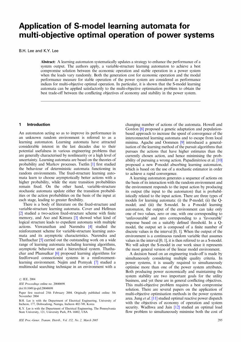
This optimisation problem can be solved by usinglearning automata. The concept of learning automataapplication to the multi-objective problem is shown inFig. 1, where the random environment represents a targetsystem, which may have uncertainties and random noises.

The procedure in the learning automata is summarised asfollows:

1. Extremum points are determined by independently,minimising each single objective function and r actions areappropriately selected over the space enclosed by theextremum points.

2. The probabilities of r actions (probability vector:

pðnÞ ¼ fp1ðnÞ;p2ðnÞ; � � � ;prðnÞgt) are updated accordingto the degree of favourableness of the response in therandom environment (In general, the initial probabilities areof equal probability in (4) and (5)).

3. An action is randomly selected under the probabilityvector of r actions and applied to the environment.

4. The random environment responds to the input and theperformance of J(x) is assessed by evaluating the outputaccording to the given criteria.

5. The above steps 2, 3 and 4 are repeated until theprobability vector converges to a fixed value.

6. After convergence, the action that has the highestprobability in a learning automaton is the best compromisesolution that simultaneously satisfies the multi-criteria.

To illustrate this concept, two objective functions areconsidered namely: (i) the generation cost for economicoperation; and (ii) a modal performance measure for stableoperation of the power system.

3.2 Multi-objective functions

3.2.1 Economic operation of a power sys-tem: The first goal of power system operation is tominimise the operation cost. For simplicity of analysis, it isassumed that the cost function for economic operation isgiven by the total summation of the generation fuel costs,which can be expressed as a quadratic function of thegenerating powers:

J1ðPsgÞ ¼Xk2G

ðak þ bkPk þ ckP 2k Þ ð8Þ

where G is a set of indices of generator buses including theswing bus, J1 is the generation cost function, Psg is the realpowers of the generator buses including the swing bus, and

ak,bk and ck are generation cost parameters. The steepestdescent method [16] is used to minimise this function.

3.2.2 Stable operation of a power system: -The second important goal is to enhance the dynamicstability of a power system. The following modal perfor-mance measure is used for a rapid decay of the modeenvelopes derived from the mathematical model fordynamic stability [13]:

J2ðPsgÞ ¼Xn

j¼0JSj ð9Þ

with

JSj ¼Z T

0

Xn

i¼1zt

j;iWjzj;i � dt for the j th state ð10Þ

where T is an integration time interval, z(t) is the outputerror from a reference, zj,i is the ith mode of the componentof z(t) that depends on the jth state of the state vector xðtÞin the system dynamics, Wj is a weighting matrix for the jthstate, and superscript (*) denotes complex conjugate. Adetailed description of the mathematical model for thedynamic stability can be referred to in [13]. The gradient ofthe modal performance measure has been evaluated in [13].We will use the steepest descent method [16] to obtain theminimum of the performance measure J2.

4 Simulation

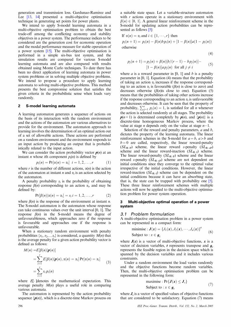
4.1 Power system modelThe system used for simulation is the six-bus power systemshown in Fig. 2. Buses 1 and 2 are generator buses andothers are load buses. The line data and the initial data forgeneration and load of the power system are given inTables 1 and 2, respectively. Bus 1 is a swing bus. It isassumed that loads contain uncertainty and are Gaussian

probabilisticaction generation( r actions set )

random environment(plant with

random variables)

learning automaton(updating of action

probability vector P )

�

input

βn

β2β1

multiple responses(n objectives)

Fig. 1 Application of a learning automaton to the multi-objectiveoptimisation problem

G

G1

2

34

6 5 26

34

Fig. 2 The six-bus power system

Table 1: Line data for the six-bus power system

Line From bus To bus Line impedancep.u.

R X

1 1 6 0.135 0.962

2 1 4 0.100 0.756

3 4 6 0.120 0.795

4 5 6 0.110 0.873

5 2 5 0.142 0.983

6 2 3 0.181 1.210

7 3 4 0.050 0.410

IEE Proc.-Gener. Transm. Distrib., Vol. 152, No. 2, March 2005 297

with a 3% standard deviation and that the power factor ateach bus remains constant. The model for the analysis ofthe modal performance measure includes the nonlinearmachine model with a two-axis representation of thegenerator and the IEEE type-1 excitation system [13]. Thedata for the generation cost parameters are given in Table 3.

4.2 Performance evaluationIf the power of generator 2 is specified, the power ofgenerator 1 can be determined through load flow. There-fore, the generation dispatch in this system is to determinethe real power of generator 2. For the case considered, the

real power (PminG2E) of generator 2 to safely minimise the

generation cost is 0.072 p.u., whereas the real power (PminG2S)

to safely minimise the modal performance measure for theenhancement of power system stability is 0.417 p.u. Suitablevalues of the thresholds used for determining the extent ofsatisfaction are decided by the decision maker, dependingon various conditions. Here, they are selected so that theperformance ratio, i.e. the ratio of the minimum value of thegeneration cost to the actual value of the generation cost,J1ðPmin

G2EÞ=J1ðPG2EÞ, to be 90% for economic operation and,similarly, the performance ratio of the minimum value ofthe modal performance measure to the actual value of themodal performance measure, J2ðPmin

G2SÞ=J2ðPG2SÞ, to be 50%for stable operation. Each performance ratio is normalisedto give a sigmoid output between zero and one around thethreshold value. The sum of the performance ratios areadded as an input to generate the response b(n), which is amonotonically decreasing sigmoid function with one-half at

the threshold point. As the ratios of the performancemeasures become greater than the given thresholds, thepower system operation becomes more favourable and thevalue of b(n) approaches zero. Similarly, as the performanceratios become less than the given thresholds, the powersystem operation becomes less favourable and the value ofb(n) approaches one.

Since the power system operation in this model dependson the generation power of generator 2, the generationpower of generator 2 can be considered as the action of thelearning automaton. The interval between Pmin

G2E and PminG2S is

considered as the range of actions that can take place and itis discretised with equal increments to give ten candidatecompromise solutions. The values (PG2) of the actions areshown in Table 4. The problem of solving for a bestcompromise solution that simultaneously satisfies both theeconomic operation criterion and the stable operationcriterion is reduced to that of determining the best action tosatisfy the given criteria in the probabilistic sense. Thesystem is under a random environment where theuncertainly of the load is represented by a normallydistributed random variable with a 3% standard deviation.The random loads are generated repeatedly and the powersystem is analysed for the given values of the loads. Thenthe learning automata learn to choose better actions toimprove the performance, making the solution converge toa best compromise solution. The reward parameter a andthe penalty parameter b are selected suitably by trial anderror. If the values of a and b are large, the trajectoriesconverge with a large oscillation. On the other hand, if thevalues are small, the trajectories are smooth, but convergeslowly.

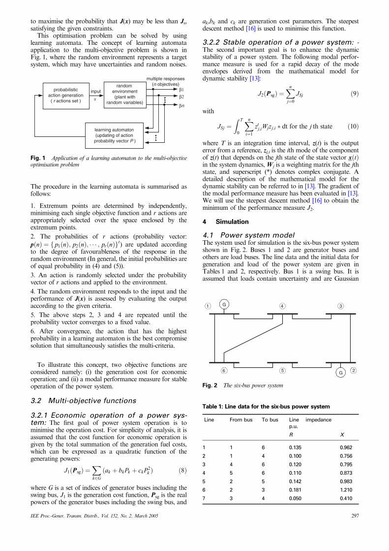
4.3 Simulation resultsThe simulation results for the SLR–P scheme witha¼ b¼ 0.02 are shown in Fig. 3. The probability of action5 converges to one as the trial number n increases and this

Table 2: Initial data of generation and load of the system(unit: p.u.)

Bus Voltage magnitude Voltage angle P Q

1 1.0 0.0

2 1.0 0.32

3 �0.27 �0.06

4 0.00 0.00

5 �0.19 �0.05

6 �0.28 �0.03

Table 3: Generation cost data

Cost coefficients ofgenerator 1

Cost coefficients ofgenerator 2

a1 52.0 a2 88.0

b1 1.12 b2 1.91

c1 0.0021 c2 0.0035

0 100 200 300 4000

0.2

0.4

0.6

0.8

1.0

M (n)

p10

p5

prob

abili

ty a

nd M

(n)

n

Fig. 3 Probabilities of actions and average penalty in the SLR–P

scheme

Table 4 PG2 values of actions. (unit: p.u.)

Actions Action 1 Action 2 Action 3 Action 4 Action 5 Action 6

PG2 0.072 0.106 0.141 0.175 0.210 0.244

Actions Action 7 Action 8 Action 9 Action 10 Action 11

PG2 0.279 0.313 0.348 0.382 0.417

298 IEE Proc.-Gener. Transm. Distrib., Vol. 152, No. 2, March 2005

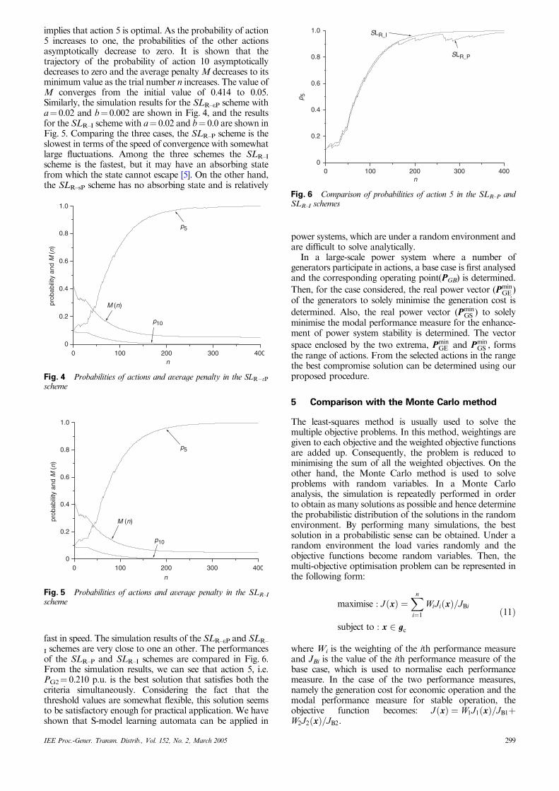
implies that action 5 is optimal. As the probability of action5 increases to one, the probabilities of the other actionsasymptotically decrease to zero. It is shown that thetrajectory of the probability of action 10 asymptoticallydecreases to zero and the average penalty M decreases to itsminimum value as the trial number n increases. The value ofM converges from the initial value of 0.414 to 0.05.Similarly, the simulation results for the SLR–eP scheme witha¼ 0.02 and b¼ 0.002 are shown in Fig. 4, and the resultsfor the SLR–I scheme with a¼ 0.02 and b¼ 0.0 are shown inFig. 5. Comparing the three cases, the SLR–P scheme is theslowest in terms of the speed of convergence with somewhatlarge fluctuations. Among the three schemes the SLR–I

scheme is the fastest, but it may have an absorbing statefrom which the state cannot escape [5]. On the other hand,the SLR–sP scheme has no absorbing state and is relatively

fast in speed. The simulation results of the SLR–eP and SLR–

I schemes are very close to one an other. The performancesof the SLR–P and SLR–I schemes are compared in Fig. 6.From the simulation results, we can see that action 5, i.e.PG2¼ 0.210 p.u. is the best solution that satisfies both thecriteria simultaneously. Considering the fact that thethreshold values are somewhat flexible, this solution seemsto be satisfactory enough for practical application. We haveshown that S-model learning automata can be applied in

power systems, which are under a random environment andare difficult to solve analytically.

In a large-scale power system where a number ofgenerators participate in actions, a base case is first analysedand the corresponding operating point(PGB) is determined.

Then, for the case considered, the real power vector (PminGE )

of the generators to solely minimise the generation cost is

determined. Also, the real power vector (PminGS ) to solely

minimise the modal performance measure for the enhance-ment of power system stability is determined. The vector

space enclosed by the two extrema, PminGE and Pmin

GS , formsthe range of actions. From the selected actions in the rangethe best compromise solution can be determined using ourproposed procedure.

5 Comparison with the Monte Carlo method

The least-squares method is usually used to solve themultiple objective problems. In this method, weightings aregiven to each objective and the weighted objective functionsare added up. Consequently, the problem is reduced tominimising the sum of all the weighted objectives. On theother hand, the Monte Carlo method is used to solveproblems with random variables. In a Monte Carloanalysis, the simulation is repeatedly performed in orderto obtain as many solutions as possible and hence determinethe probabilistic distribution of the solutions in the randomenvironment. By performing many simulations, the bestsolution in a probabilistic sense can be obtained. Under arandom environment the load varies randomly and theobjective functions become random variables. Then, themulti-objective optimisation problem can be represented inthe following form:

maximise : JðxÞ ¼Xn

i¼1WiJiðxÞ=JBi

subject to : x 2 gc

ð11Þ

where Wi is the weighting of the ith performance measureand JBi is the value of the ith performance measure of thebase case, which is used to normalise each performancemeasure. In the case of the two performance measures,namely the generation cost for economic operation and themodal performance measure for stable operation, theobjective function becomes: JðxÞ ¼ W1J1ðxÞ=JB1þW2J2ðxÞ=JB2.

0 100 200 300 4000

0.2

0.4

0.6

0.8

1.0

M (n)

p10

p5

prob

abili

ty a

nd M

(n)

n

Fig. 4 Probabilities of actions and average penalty in the SLR�ePscheme

0 100 200 300 4000

0.2

0.4

0.6

0.8

1.0

M (n)

p10

p5

prob

abili

ty a

nd M

(n)

n

Fig. 5 Probabilities of actions and average penalty in the SLR–I

scheme

0 100 200 300 4000

0.2

0.4

0.6

0.8

1.0 SLR_I

SLR_P

p 5

n

Fig. 6 Comparison of probabilities of action 5 in the SLR–P andSLR–I schemes

IEE Proc.-Gener. Transm. Distrib., Vol. 152, No. 2, March 2005 299

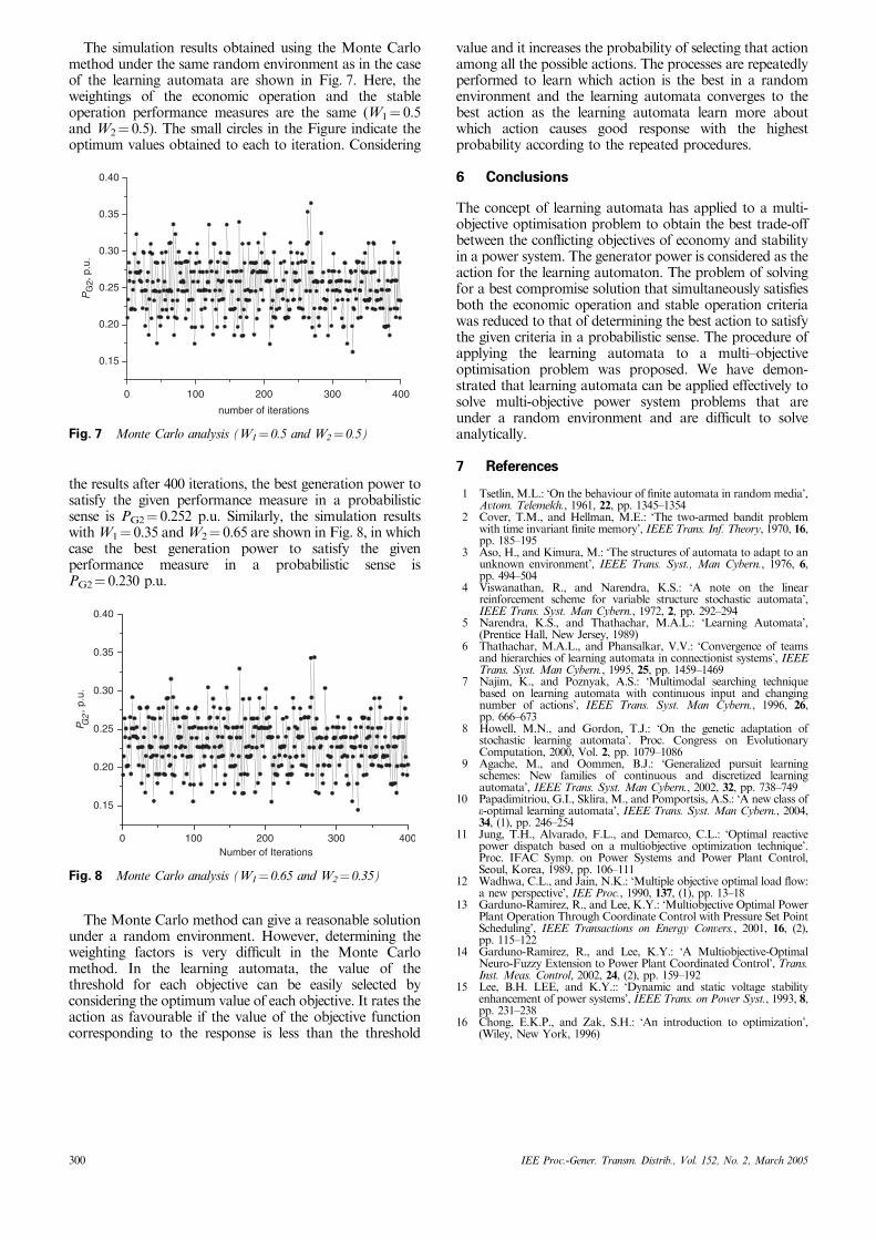
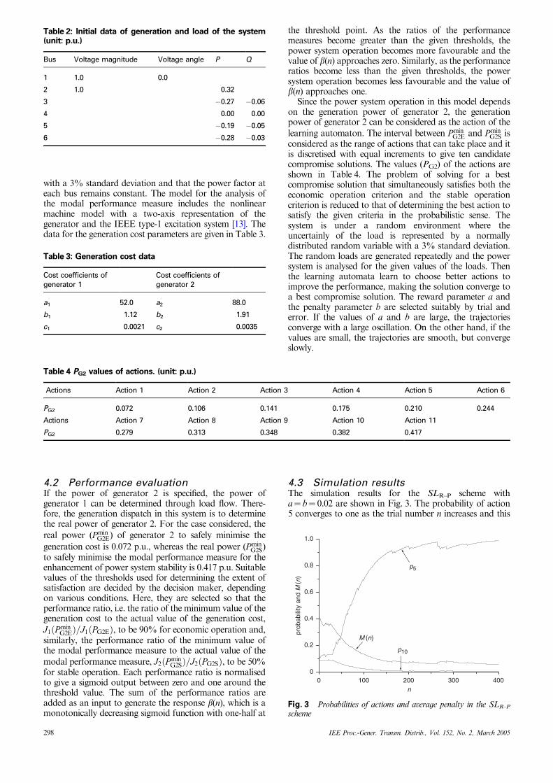
The simulation results obtained using the Monte Carlomethod under the same random environment as in the caseof the learning automata are shown in Fig. 7. Here, theweightings of the economic operation and the stableoperation performance measures are the same (W1¼ 0.5and W2¼ 0.5). The small circles in the Figure indicate theoptimum values obtained to each to iteration. Considering

the results after 400 iterations, the best generation power tosatisfy the given performance measure in a probabilisticsense is PG2¼ 0.252 p.u. Similarly, the simulation resultswith W1¼ 0.35 and W2¼ 0.65 are shown in Fig. 8, in whichcase the best generation power to satisfy the givenperformance measure in a probabilistic sense isPG2¼ 0.230 p.u.

The Monte Carlo method can give a reasonable solutionunder a random environment. However, determining theweighting factors is very difficult in the Monte Carlomethod. In the learning automata, the value of thethreshold for each objective can be easily selected byconsidering the optimum value of each objective. It rates theaction as favourable if the value of the objective functioncorresponding to the response is less than the threshold

value and it increases the probability of selecting that actionamong all the possible actions. The processes are repeatedlyperformed to learn which action is the best in a randomenvironment and the learning automata converges to thebest action as the learning automata learn more aboutwhich action causes good response with the highestprobability according to the repeated procedures.

6 Conclusions

The concept of learning automata has applied to a multi-objective optimisation problem to obtain the best trade-offbetween the conflicting objectives of economy and stabilityin a power system. The generator power is considered as theaction for the learning automaton. The problem of solvingfor a best compromise solution that simultaneously satisfiesboth the economic operation and stable operation criteriawas reduced to that of determining the best action to satisfythe given criteria in a probabilistic sense. The procedure ofapplying the learning automata to a multi–objectiveoptimisation problem was proposed. We have demon-strated that learning automata can be applied effectively tosolve multi-objective power system problems that areunder a random environment and are difficult to solveanalytically.

7 References

1 Tsetlin, M.L.: ‘On the behaviour of finite automata in randommedia’,Avtom. Telemekh., 1961, 22, pp. 1345–1354

2 Cover, T.M., and Hellman, M.E.: ‘The two-armed bandit problemwith time invariant finite memory’, IEEE Trans. Inf. Theory, 1970, 16,pp. 185–195

3 Aso, H., and Kimura, M.: ‘The structures of automata to adapt to anunknown environment’, IEEE Trans. Syst., Man Cybern., 1976, 6,pp. 494–504

4 Viswanathan, R., and Narendra, K.S.: ‘A note on the linearreinforcement scheme for variable structure stochastic automata’,IEEE Trans. Syst. Man Cybern., 1972, 2, pp. 292–294

5 Narendra, K.S., and Thathachar, M.A.L.: ‘Learning Automata’,(Prentice Hall, New Jersey, 1989)

6 Thathachar, M.A.L., and Phansalkar, V.V.: ‘Convergence of teamsand hierarchies of learning automata in connectionist systems’, IEEETrans. Syst. Man Cybern., 1995, 25, pp. 1459–1469

7 Najim, K., and Poznyak, A.S.: ‘Multimodal searching techniquebased on learning automata with continuous input and changingnumber of actions’, IEEE Trans. Syst. Man Cybern., 1996, 26,pp. 666–673

8 Howell, M.N., and Gordon, T.J.: ‘On the genetic adaptation ofstochastic learning automata’. Proc. Congress on EvolutionaryComputation, 2000, Vol. 2, pp. 1079–1086

9 Agache, M., and Oommen, B.J.: ‘Generalized pursuit learningschemes: New families of continuous and discretized learningautomata’, IEEE Trans. Syst. Man Cybern., 2002, 32, pp. 738–749

10 Papadimitriou, G.I., Sklira, M., and Pomportsis, A.S.: ‘A new class ofe-optimal learning automata’, IEEE Trans. Syst. Man Cybern., 2004,34, (1), pp. 246–254

11 Jung, T.H., Alvarado, F.L., and Demarco, C.L.: ‘Optimal reactivepower dispatch based on a multiobjective optimization technique’.Proc. IFAC Symp. on Power Systems and Power Plant Control,Seoul, Korea, 1989, pp. 106–111

12 Wadhwa, C.L., and Jain, N.K.: ‘Multiple objective optimal load flow:a new perspective’, IEE Proc., 1990, 137, (1), pp. 13–18

13 Garduno-Ramirez, R., and Lee, K.Y.: ‘Multiobjective Optimal PowerPlant Operation Through Coordinate Control with Pressure Set PointScheduling’, IEEE Transactions on Energy Convers., 2001, 16, (2),pp. 115–122

14 Garduno-Ramirez, R., and Lee, K.Y.: ‘A Multiobjective-OptimalNeuro-Fuzzy Extension to Power Plant Coordinated Control’, Trans.Inst. Meas. Control, 2002, 24, (2), pp. 159–192

15 Lee, B.H. LEE, and K.Y.:: ‘Dynamic and static voltage stabilityenhancement of power systems’, IEEE Trans. on Power Syst., 1993, 8,pp. 231–238

16 Chong, E.K.P., and Zak, S.H.: ‘An introduction to optimization’,(Wiley, New York, 1996)

0 100 200 300 400

0.15

0.20

0.25

0.30

0.35

0.40

P G2 ,

p.u

.

Number of Iterations

Fig. 8 Monte Carlo analysis (W1¼ 0.65 and W2¼ 0.35)

0 100 200 300 400

0.15

0.20

0.25

0.30

0.35

0.40

PG

2, p

.u.

number of iterations

Fig. 7 Monte Carlo analysis (W1¼ 0.5 and W2¼ 0.5)

300 IEE Proc.-Gener. Transm. Distrib., Vol. 152, No. 2, March 2005