Applying data mining to telecom churn management

Applying data mining to telecom churn management

Shin-Yuan Hung a, David C. Yen b,*, Hsiu-Yu Wang c

a Department of Information Management, National Chung Cheng University, Chia-Yi 62117, Taiwan, ROCb Department of DSC and MIS, Miami University, 309 Upham, Oxford, OH 45056, USA

c Department of Information Management, National Chung Cheng University, Chia-Yi 62117, Taiwan, ROC

Abstract

Taiwan deregulated its wireless telecommunication services in 1997. Fierce competition followed, and churn management becomes a major

focus of mobile operators to retain subscribers via satisfying their needs under resource constraints. One of the challenges is churner prediction.

Through empirical evaluation, this study compares various data mining techniques that can assign a ‘propensity-to-churn’ score periodically to

each subscriber of a mobile operator. The results indicate that both decision tree and neural network techniques can deliver accurate churn

prediction models by using customer demographics, billing information, contract/service status, call detail records, and service change log.

q 2005 Elsevier Ltd. All rights reserved.

Keywords: Churn management; Wireless telecommunication; Data mining; Decision tree; Neural network

1. Introduction

Taiwan opened its wireless telecommunication services

market in 1997, with licenses granted to six mobile operators.

Competition has been fierce from this point. For any

acquisition activity, mobile operators need to have significant

network investment to provide ubiquitous access and quality

communications. The market was saturated within 5 years, and

mergers and acquisitions reduced the number of mobile

operators from six to four by the end of 2003.

When the market is saturated, the pool of ‘available

customers’ is limited and an operator has to shift from its

acquisition strategy to retention because the cost of acquisition

is typically five times higher than retention. As Mattersion

(2001) noted, ‘For many telecom executives, figuring out how

to deal with Churn is turning out to be the key to very survival

of their organizations’.

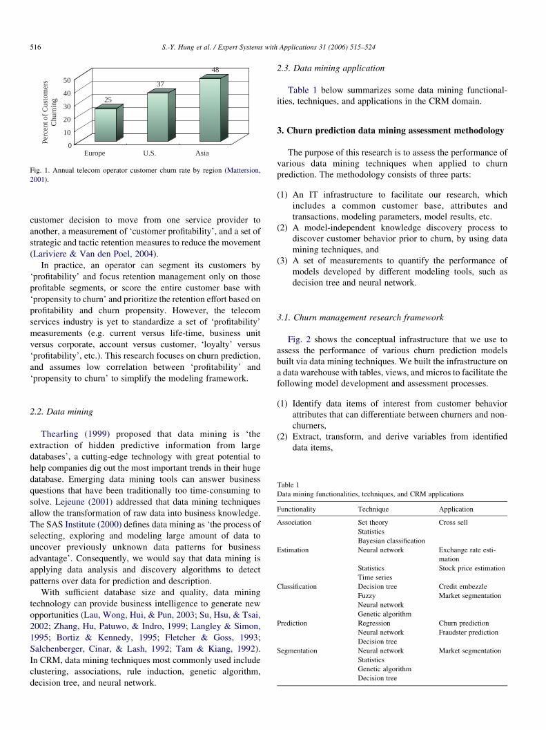
Based on marketing research (Berson, Smith, & Thearling,

2000), the average churn of a wireless operator is about 2% per

month. That is, a carrier lost about a quarter of its customer

base each year. Furthermore, Fig. 1 suggests that Asian

telecom providers face a more challenging customer churn than

those in other parts of the world.

0957-4174/$ - see front matter q 2005 Elsevier Ltd. All rights reserved.

doi:10.1016/j.eswa.2005.09.080

* Corresponding author.

E-mail addresses: [email protected] (S.-Y. Hung), yendc@muoho.

edu (D.C. Yen), [email protected] (H.-Y. Wang).

From a business intelligence perspective, churn manage-

ment process under the customer relationship management

(CRM) framework consists of two major analytical modeling

efforts: predicting those who are about to churn and assessing

the most effective way that an operator can react (including ‘do

nothing’) in terms of retention. This research focuses on the

former. It intends to illustrate how to apply IT technology to

facilitate telecom churn management. Specifically, this

research uses data mining techniques to find a best model of

predictive churn from data warehouse to prevent the customers

turnover, further to enhance the competitive edge.

The remainder of this paper is organized as follows. Section

2 defines some basic concepts (and rationale) that we use in the

research, Section 3 describes our research methodology, and

Section 4 presents the findings. Section 5 concludes this paper.

2. Basic concept

2.1. Churn management

Berson et al. (2000) noted that ‘customer churn’ is a term

used in the wireless telecom service industry to denote the

customer movement from one provider to another, and ‘churn

management’ is a term that describes an operator’s process to

retain profitable customers. Similarly, Kentrias (2001) thought

that the term churn management in the telecom services

industry is used to describe the procedure of securing the most

important customers for a company. In essence, proper

customer management presumes an ability to forecast the

Expert Systems with Applications 31 (2006) 515–524

www.elsevier.com/locate/eswa

http://www.elsevier.com/locate/eswa

25

37

48

0

10

20

30

40

50

Perc

ent o

f C

usto

mer

sC

hurn

ing

Europe U.S. Asia

Fig. 1. Annual telecom operator customer churn rate by region (Mattersion,

2001).

S.-Y. Hung et al. / Expert Systems with Applications 31 (2006) 515–524516

customer decision to move from one service provider to

another, a measurement of ‘customer profitability’, and a set of

strategic and tactic retention measures to reduce the movement

(Lariviere & Van den Poel, 2004).

In practice, an operator can segment its customers by

‘profitability’ and focus retention management only on those

profitable segments, or score the entire customer base with

‘propensity to churn’ and prioritize the retention effort based on

profitability and churn propensity. However, the telecom

services industry is yet to standardize a set of ‘profitability’

measurements (e.g. current versus life-time, business unit

versus corporate, account versus customer, ‘loyalty’ versus

‘profitability’, etc.). This research focuses on churn prediction,

and assumes low correlation between ‘profitability’ and

‘propensity to churn’ to simplify the modeling framework.

Table 1

Data mining functionalities, techniques, and CRM applications

Functionality Technique Application

Association Set theory Cross sell

Statistics

Bayesian classification

Estimation Neural network Exchange rate esti-

mation

Statistics Stock price estimation

Time series

Classification Decision tree Credit embezzle

Fuzzy Market segmentation

Neural network

Genetic algorithm

Prediction Regression Churn prediction

Neural network Fraudster prediction

Decision tree

Segmentation Neural network Market segmentation

Statistics

Genetic algorithm

Decision tree

2.2. Data mining

Thearling (1999) proposed that data mining is ‘the

extraction of hidden predictive information from large

databases’, a cutting-edge technology with great potential to

help companies dig out the most important trends in their huge

database. Emerging data mining tools can answer business

questions that have been traditionally too time-consuming to

solve. Lejeune (2001) addressed that data mining techniques

allow the transformation of raw data into business knowledge.

The SAS Institute (2000) defines data mining as ‘the process of

selecting, exploring and modeling large amount of data to

uncover previously unknown data patterns for business

advantage’. Consequently, we would say that data mining is

applying data analysis and discovery algorithms to detect

patterns over data for prediction and description.

With sufficient database size and quality, data mining

technology can provide business intelligence to generate new

opportunities (Lau, Wong, Hui, & Pun, 2003; Su, Hsu, & Tsai,

2002; Zhang, Hu, Patuwo, & Indro, 1999; Langley & Simon,

1995; Bortiz & Kennedy, 1995; Fletcher & Goss, 1993;

Salchenberger, Cinar, & Lash, 1992; Tam & Kiang, 1992).

In CRM, data mining techniques most commonly used include

clustering, associations, rule induction, genetic algorithm,

decision tree, and neural network.

2.3. Data mining application

Table 1 below summarizes some data mining functional-

ities, techniques, and applications in the CRM domain.

3. Churn prediction data mining assessment methodology

The purpose of this research is to assess the performance of

various data mining techniques when applied to churn

prediction. The methodology consists of three parts:

(1) An IT infrastructure to facilitate our research, which

includes a common customer base, attributes and

transactions, modeling parameters, model results, etc.

(2) A model-independent knowledge discovery process to

discover customer behavior prior to churn, by using data

mining techniques, and

(3) A set of measurements to quantify the performance of

models developed by different modeling tools, such as

decision tree and neural network.

3.1. Churn management research framework

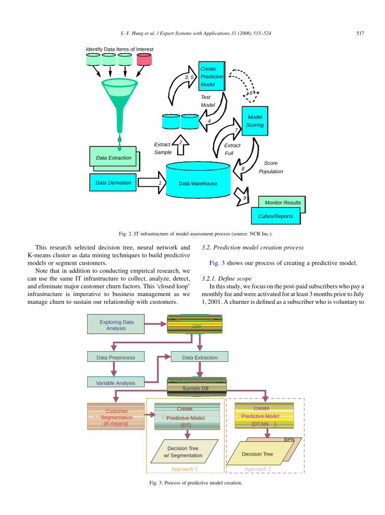
Fig. 2 shows the conceptual infrastructure that we use to

assess the performance of various churn prediction models

built via data mining techniques. We built the infrastructure on

a data warehouse with tables, views, and micros to facilitate the

following model development and assessment processes.

(1) Identify data items of interest from customer behavior

attributes that can differentiate between churners and non-

churners,

(2) Extract, transform, and derive variables from identified

data items,

Full

2

3, 5

4

6

7

8

9

Score

Population

Monitor Results

Cubes/Reports

Extract

Sample

Test

Model

Model

Scoring

Data Warehouse

Data Extraction

Data Derivation 1

Create

Predictive

Model

Identify Data Items of Interest

Extract

Fig. 2. IT infrastructure of model assessment process (source: NCR Inc.).

S.-Y. Hung et al. / Expert Systems with Applications 31 (2006) 515–524 517

This research selected decision tree, neural network and

K-means cluster as data mining techniques to build predictive

models or segment customers.

Note that in addition to conducting empirical research, we

can use the same IT infrastructure to collect, analyze, detect,

and eliminate major customer churn factors. This ‘closed loop’

infrastructure is imperative to business management as we

manage churn to sustain our relationship with customers.

DWExploring Data

Analysis

Data Preprocess

Variable Analysis

Data Extra

Sample DB

Customer

Segmentation

(K - means)

Create

Predictive Model

(DT)

Decision Tree w/ Segmentation

Approach 1

DWExploring Data

Analysis

Data Preprocess

Variable Analysis

Data Ex

Sample

CustomerSegmentation

(K-means)

Create

Predictive Mod(DT)

Decision Tree w/ Segmentation

Fig. 3. Process of predic

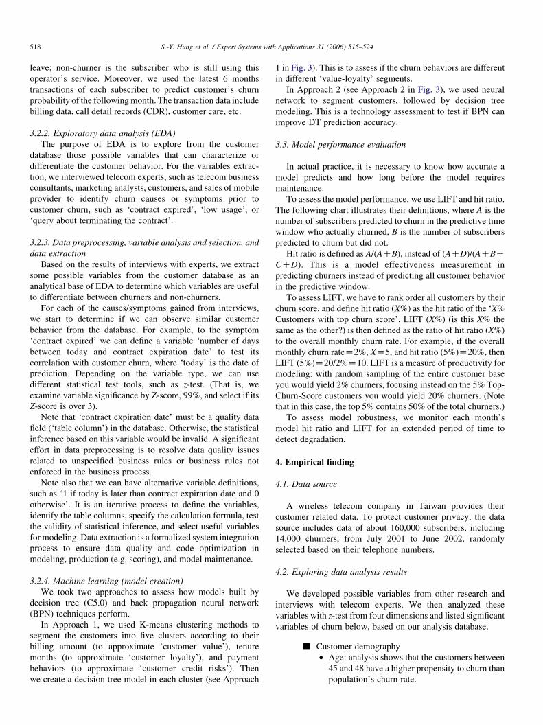
3.2. Prediction model creation process

Fig. 3 shows our process of creating a predictive model.

3.2.1. Define scope

In this study, we focus on the post-paid subscribers who pay a

monthly fee and were activated for at least 3 months prior to July

1, 2001. A churner is defined as a subscriber who is voluntary to

ction

Create

Predictive Model

(DT,NN )

Decision Tree

BPN

Approach 2

traction

DB

Create

Predictive Model

(DT,NN )el

Decision Tree

BPN

tive model creation.


leave; non-churner is the subscriber who is still using this

operator’s service. Moreover, we used the latest 6 months

transactions of each subscriber to predict customer’s churn

probability of the following month. The transaction data include

billing data, call detail records (CDR), customer care, etc.

3.2.2. Exploratory data analysis (EDA)

The purpose of EDA is to explore from the customer

database those possible variables that can characterize or

differentiate the customer behavior. For the variables extrac-

tion, we interviewed telecom experts, such as telecom business

consultants, marketing analysts, customers, and sales of mobile

provider to identify churn causes or symptoms prior to

customer churn, such as ‘contract expired’, ‘low usage’, or

‘query about terminating the contract’.

3.2.3. Data preprocessing, variable analysis and selection, and

data extraction

Based on the results of interviews with experts, we extract

some possible variables from the customer database as an

analytical base of EDA to determine which variables are useful

to differentiate between churners and non-churners.

For each of the causes/symptoms gained from interviews,

we start to determine if we can observe similar customer

behavior from the database. For example, to the symptom

‘contract expired’ we can define a variable ‘number of days

between today and contract expiration date’ to test its

correlation with customer churn, where ‘today’ is the date of

prediction. Depending on the variable type, we can use

different statistical test tools, such as z-test. (That is, we

examine variable significance by Z-score, 99%, and select if its

Z-score is over 3).

Note that ‘contract expiration date’ must be a quality data

field (‘table column’) in the database. Otherwise, the statistical

inference based on this variable would be invalid. A significant

effort in data preprocessing is to resolve data quality issues

related to unspecified business rules or business rules not

enforced in the business process.

Note also that we can have alternative variable definitions,

such as ‘1 if today is later than contract expiration date and 0

otherwise’. It is an iterative process to define the variables,

identify the table columns, specify the calculation formula, test

the validity of statistical inference, and select useful variables

for modeling. Data extraction is a formalized system integration

process to ensure data quality and code optimization in

modeling, production (e.g. scoring), and model maintenance.

3.2.4. Machine learning (model creation)

We took two approaches to assess how models built by

decision tree (C5.0) and back propagation neural network

(BPN) techniques perform.

In Approach 1, we used K-means clustering methods to

segment the customers into five clusters according to their

billing amount (to approximate ‘customer value’), tenure

months (to approximate ‘customer loyalty’), and payment

behaviors (to approximate ‘customer credit risks’). Then

we create a decision tree model in each cluster (see Approach

1 in Fig. 3). This is to assess if the churn behaviors are different

in different ‘value-loyalty’ segments.

In Approach 2 (see Approach 2 in Fig. 3), we used neural

network to segment customers, followed by decision tree

modeling. This is a technology assessment to test if BPN can

improve DT prediction accuracy.

3.3. Model performance evaluation

In actual practice, it is necessary to know how accurate a

model predicts and how long before the model requires

maintenance.

To assess the model performance, we use LIFT and hit ratio.

The following chart illustrates their definitions, where A is the

number of subscribers predicted to churn in the predictive time

window who actually churned, B is the number of subscribers

predicted to churn but did not.

Hit ratio is defined as A/(ACB), instead of (ACD)/(ACBCCCD). This is a model effectiveness measurement in

predicting churners instead of predicting all customer behavior

in the predictive window.

To assess LIFT, we have to rank order all customers by their

churn score, and define hit ratio (X%) as the hit ratio of the ‘X%

Customers with top churn score’. LIFT (X%) (is this X% the

same as the other?) is then defined as the ratio of hit ratio (X%)

to the overall monthly churn rate. For example, if the overall

monthly churn rateZ2%, XZ5, and hit ratio (5%)Z20%, then

LIFT (5%)Z20/2%Z10. LIFT is a measure of productivity for

modeling: with random sampling of the entire customer base

you would yield 2% churners, focusing instead on the 5% Top-

Churn-Score customers you would yield 20% churners. (Note

that in this case, the top 5% contains 50% of the total churners.)

To assess model robustness, we monitor each month’s

model hit ratio and LIFT for an extended period of time to

detect degradation.

4. Empirical finding

4.1. Data source

A wireless telecom company in Taiwan provides their

customer related data. To protect customer privacy, the data

source includes data of about 160,000 subscribers, including

14,000 churners, from July 2001 to June 2002, randomly

selected based on their telephone numbers.

4.2. Exploring data analysis results

We developed possible variables from other research and

interviews with telecom experts. We then analyzed these

variables with z-test from four dimensions and listed significant

variables of churn below, based on our analysis database.

- Customer demography

† Age: analysis shows that the customers between

45 and 48 have a higher propensity to churn than

population’s churn rate.

9.6%

1.2%

1.4%

1.6%

C2

C5


† Tenure: customers with 25 – 30 months tenure

have a high propensity to churn. A possible

cause is that most subscription plans have a

2-year contract period.

† Gender: churn probability for corporate

accounts is higher than others. A possible

cause is that when employees quit, they lose

corporate subsidy in mobile services.

- Bill and payment analysis

† Monthly fee: the churn probability is higher for

customers with a monthly fee less than $100 NT

or between $520 and $550.

† Billing amount: the churn probability tends to be

higher for customers whose average billing

amount over 6 months is less than or equal to

$190 NT.

† Count of overdue payment: the churn probability

is higher for customers with less than four counts

of overdue payments in the past 6 months. In

Taiwan, if the payment is 2 months overdue, the

mobile operator will most likely suspend the

mobile service until fully paid. This may cause

customer dissatisfaction and churn.

- Call detail records analysis

† In-net call duration: customers who don’t often

make phone calls to others in the same operator’s

mobile network are more likely to churn. In-net

unit price is relatively lower than that of other call

types. Price-sensitive subscribers may leave for

the mobile operator his/her friends use.

† Call type: customers who often make PSTN or

IDD calls are more likely to churn than those who

make more mobile calls.

- Customer care/service analysis

† MSISDN change count: customers who have

changed their phone number or made two or more

changes in account information are more likely to

churn.

† Count of bar and suspend: customers who have

ever been barred or suspended are more likely to

churn. In general, a subscriber will be barred or

suspended by the mobile operators due to

overdue payments.

Table 2 summarizes variables significant to differentiate

between churners and non-churners from EDA. We use those

variables for machine learning.

Table 2

Significant variables of churn

Dimension Items

Demography Gender, age, area tenure

CDR Inbound call, outbound call, demestric call,

Bill/payment Bill amount, payment, overdue payment, monthly fee

Custer service Inquire, phone no changed, bar/suspend

4.3. Customer segmentation

To segment customers by loyalty, contribution, and usage,

we selected bill amount, tenure, MOU (outbound call usage),

MTU (inbound call usage), and payment rate as variables and

used K-Means to model the customers into five clusters. To

generate roughly the same number of subscribers in each of the

five clusters, we divided the customers equally into three

segments high, medium, and low for each variable.

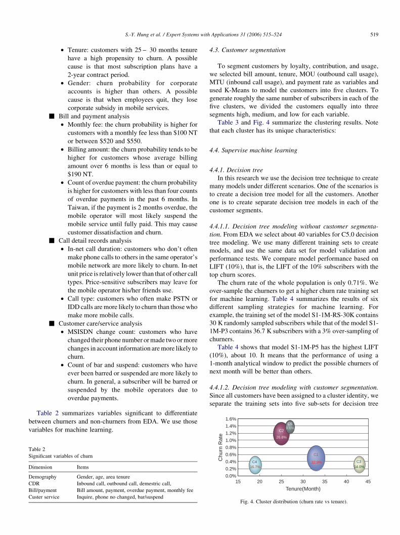
Table 3 and Fig. 4 summarize the clustering results. Note

that each cluster has its unique characteristics:

4.4. Supervise machine learning

4.4.1. Decision tree

In this research we use the decision tree technique to create

many models under different scenarios. One of the scenarios is

to create a decision tree model for all the customers. Another

one is to create separate decision tree models in each of the

customer segments.

4.4.1.1. Decision tree modeling without customer segmenta-

tion. From EDA we select about 40 variables for C5.0 decision

tree modeling. We use many different training sets to create

models, and use the same data set for model validation and

performance tests. We compare model performance based on

LIFT (10%), that is, the LIFT of the 10% subscribers with the

top churn scores.

The churn rate of the whole population is only 0.71%. We

over-sample the churners to get a higher churn rate training set

for machine learning. Table 4 summarizes the results of six

different sampling strategies for machine learning. For

example, the training set of the model S1-1M-RS-30K contains

30 K randomly sampled subscribers while that of the model S1-

1M-P3 contains 36.7 K subscribers with a 3% over-sampling of

churners.

Table 4 shows that model S1-1M-P5 has the highest LIFT

(10%), about 10. It means that the performance of using a

1-month analytical window to predict the possible churners of

next month will be better than others.

4.4.1.2. Decision tree modeling with customer segmentation.

Since all customers have been assigned to a cluster identity, we

separate the training sets into five sub-sets for decision tree

26.8%

32.9%14.0%16.7%

0.0%

0.2%

0.4%

0.6%

0.8%

1.0%

15 20 25 30 35 40 45

Tenure(Month)

Chu

rn R

ate

C4 C3

C1

Fig. 4. Cluster distribution (churn rate vs tenure).

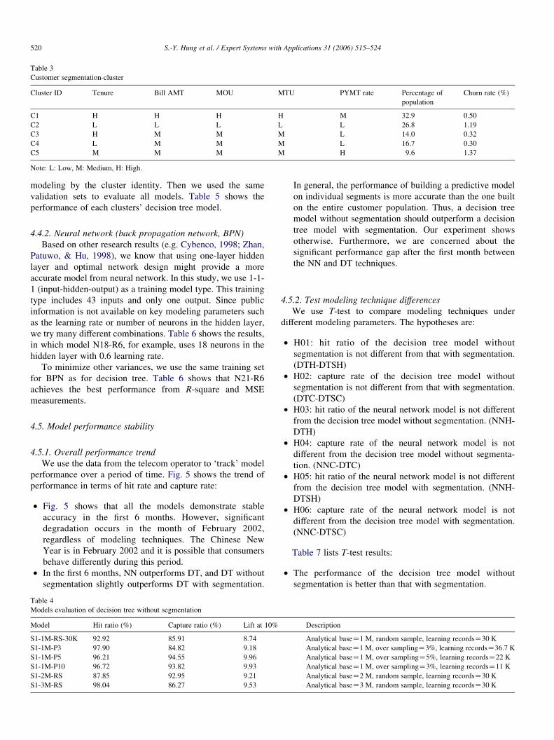
Table 3

Customer segmentation-cluster

Cluster ID Tenure Bill AMT MOU MTU PYMT rate Percentage of

population

Churn rate (%)

C1 H H H H M 32.9 0.50

C2 L L L L L 26.8 1.19

C3 H M M M L 14.0 0.32

C4 L M M M L 16.7 0.30

C5 M M M M H 9.6 1.37

Note: L: Low, M: Medium, H: High.


modeling by the cluster identity. Then we used the same

validation sets to evaluate all models. Table 5 shows the

performance of each clusters’ decision tree model.

4.4.2. Neural network (back propagation network, BPN)

Based on other research results (e.g. Cybenco, 1998; Zhan,

Patuwo, & Hu, 1998), we know that using one-layer hidden

layer and optimal network design might provide a more

accurate model from neural network. In this study, we use 1-1-

1 (input-hidden-output) as a training model type. This training

type includes 43 inputs and only one output. Since public

information is not available on key modeling parameters such

as the learning rate or number of neurons in the hidden layer,

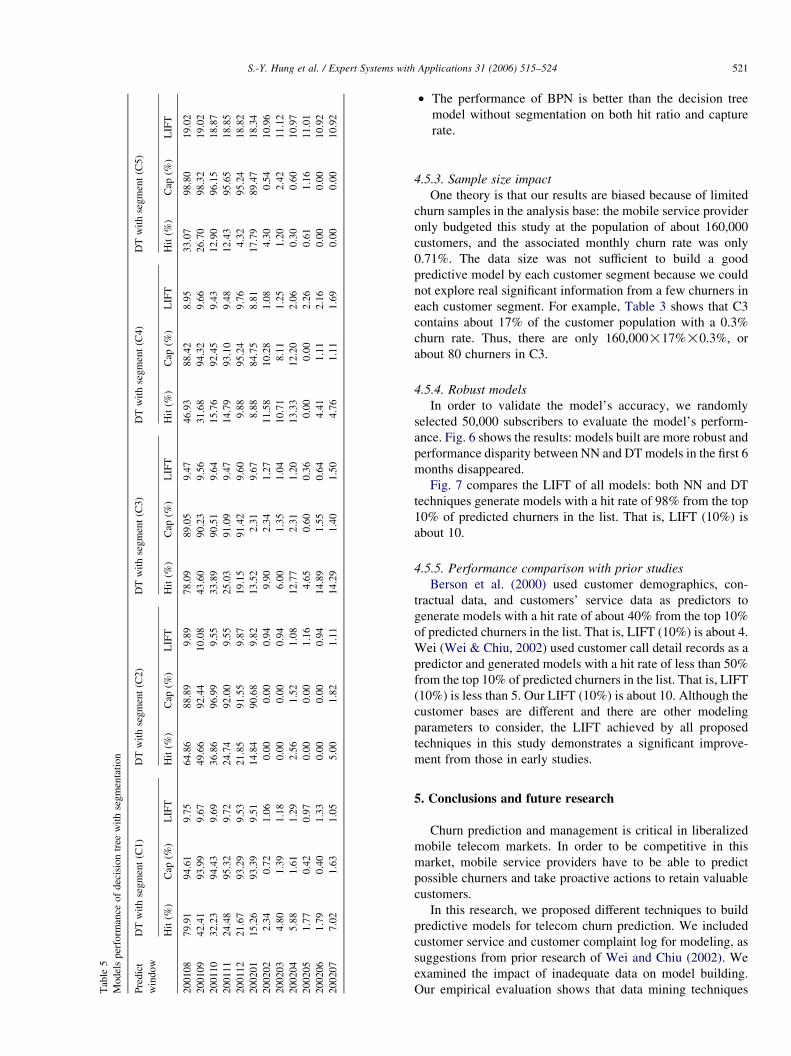
we try many different combinations. Table 6 shows the results,

in which model N18-R6, for example, uses 18 neurons in the

hidden layer with 0.6 learning rate.

To minimize other variances, we use the same training set

for BPN as for decision tree. Table 6 shows that N21-R6

achieves the best performance from R-square and MSE

measurements.

4.5. Model performance stability

4.5.1. Overall performance trend

We use the data from the telecom operator to ‘track’ model

performance over a period of time. Fig. 5 shows the trend of

performance in terms of hit rate and capture rate:

† Fig. 5 shows that all the models demonstrate stable

accuracy in the first 6 months. However, significant

degradation occurs in the month of February 2002,

regardless of modeling techniques. The Chinese New

Year is in February 2002 and it is possible that consumers

behave differently during this period.

† In the first 6 months, NN outperforms DT, and DT without

segmentation slightly outperforms DT with segmentation.

Table 4

Models evaluation of decision tree without segmentation

Model Hit ratio (%) Capture ratio (%) Lift at 10%

S1-1M-RS-30K 92.92 85.91 8.74

S1-1M-P3 97.90 84.82 9.18

S1-1M-P5 96.21 94.55 9.96

S1-1M-P10 96.72 93.82 9.93

S1-2M-RS 87.85 92.95 9.21

S1-3M-RS 98.04 86.27 9.53

In general, the performance of building a predictive model

on individual segments is more accurate than the one built

on the entire customer population. Thus, a decision tree

model without segmentation should outperform a decision

tree model with segmentation. Our experiment shows

otherwise. Furthermore, we are concerned about the

significant performance gap after the first month between

the NN and DT techniques.

4.5.2. Test modeling technique differences

We use T-test to compare modeling techniques under

different modeling parameters. The hypotheses are:

† H01: hit ratio of the decision tree model without

segmentation is not different from that with segmentation.

(DTH-DTSH)

† H02: capture rate of the decision tree model without

segmentation is not different from that with segmentation.

(DTC-DTSC)

† H03: hit ratio of the neural network model is not different

from the decision tree model without segmentation. (NNH-

DTH)

† H04: capture rate of the neural network model is not

different from the decision tree model without segmenta-

tion. (NNC-DTC)

† H05: hit ratio of the neural network model is not different

from the decision tree model with segmentation. (NNH-

DTSH)

† H06: capture rate of the neural network model is not

different from the decision tree model with segmentation.

(NNC-DTSC)

Table 7 lists T-test results:

† The performance of the decision tree model without

segmentation is better than that with segmentation.

Description

Analytical baseZ1 M, random sample, learning recordsZ30 K

Analytical baseZ1 M, over samplingZ3%, learning recordsZ36.7 K

Analytical baseZ1 M, over samplingZ5%, learning recordsZ22 K

Analytical baseZ1 M, over samplingZ3%, learning recordsZ11 K



Tab

le5

Mo

del

sp

erfo

rman

ceo

fd

ecis

ion

tree

wit

hse

gm

enta

tion

Pre

dic

t

win

do

w

DT

wit

hse

gm

ent

(C1

)D

Tw

ith

seg

men

t(C

2)

DT

wit

hse

gm

ent

(C3

)D

Tw

ith

seg

men

t(C

4)

DT

wit

hse

gm

ent

(C5

)

Hit

(%)

Cap

(%)

LIF

TH

it(%

)C

ap(%

)L

IFT

Hit

(%)

Cap

(%)

LIF

TH

it(%

)C

ap(%

)L

IFT

Hit

(%)

Cap

(%)

LIF

T

20

010

87

9.9

19

4.6

19

.75

64

.86

88

.89

9.8

97

8.0

98

9.0

59

.47

46

.93

88

.42

8.9

53

3.0

79

8.8

01

9.0

2

20

010

94

2.4

19

3.9

99

.67

49

.66

92

.44

10

.08

43

.60

90

.23

9.5

63

1.6

89

4.3

29

.66

26

.70

98

.32

19

.02

20

011

03

2.2

39

4.4

39

.69

36

.86

96

.99

9.5

53

3.8

99

0.5

19

.64

15

.76

92

.45

9.4

31

2.9

09

6.1

51

8.8

7

20

011

12

4.4

89

5.3

29

.72

24

.74

92

.00

9.5

52

5.0

39

1.0

99

.47

14

.79

93

.10

9.4

81

2.4

39

5.6

51

8.8

5

20

011

22

1.6

79

3.2

99

.53

21

.85

91

.55

9.8

71

9.1

59

1.4

29

.60

9.8

89

5.2

49

.76

4.3

29

5.2

41

8.8

2

20

020

11

5.2

69

3.3

99

.51

14

.84

90

.68

9.8

21

3.5

22

.31

9.6

78

.88

84

.75

8.8

11

7.7

98

9.4

71

8.3

4

20

020

22

.34

0.7

21

.06

0.0

00

.00

0.9

49

.90

2.3

41

.27

11

.58

10

.28

1.0

84

.30

0.5

41

0.9

6

20

020

34

.80

1.3

91

.18

0.0

00

.00

0.9

46

.00

1.3

51

.04

10

.71

8.1

11

.25

1.2

02

.42

11

.12

20

020

45

.88

1.6

11

.29

2.5

61

.52

1.0

81

2.7

72

.31

1.2

01

3.3

31

2.2

02

.06

0.3

00

.60

10

.97

20

020

51

.77

0.4

20

.97

0.0

00

.00

1.1

64

.65

0.6

00

.36

0.0

00

.00

2.2

60

.61

1.1

61

1.0

1

20

020

61

.79

0.4

01

.33

0.0

00

.00

0.9

41

4.8

91

.55

0.6

44

.41

1.1

12

.16

0.0

00

.00

10

.92

20

020

77

.02

1.6

31

.05

5.0

01

.82

1.1

11

4.2

91

.40

1.5

04

.76

1.1

11

.69

0.0

00

.00

10

.92


† The performance of BPN is better than the decision tree

model without segmentation on both hit ratio and capture

rate.

4.5.3. Sample size impact

One theory is that our results are biased because of limited

churn samples in the analysis base: the mobile service provider

only budgeted this study at the population of about 160,000

customers, and the associated monthly churn rate was only

0.71%. The data size was not sufficient to build a good

predictive model by each customer segment because we could

not explore real significant information from a few churners in

each customer segment. For example, Table 3 shows that C3

contains about 17% of the customer population with a 0.3%

churn rate. Thus, there are only 160,000!17%!0.3%, or

about 80 churners in C3.

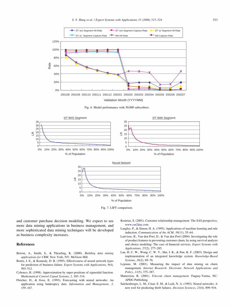
4.5.4. Robust models

In order to validate the model’s accuracy, we randomly

selected 50,000 subscribers to evaluate the model’s perform-

ance. Fig. 6 shows the results: models built are more robust and

performance disparity between NN and DT models in the first 6

months disappeared.

Fig. 7 compares the LIFT of all models: both NN and DT

techniques generate models with a hit rate of 98% from the top

10% of predicted churners in the list. That is, LIFT (10%) is

about 10.

4.5.5. Performance comparison with prior studies

Berson et al. (2000) used customer demographics, con-

tractual data, and customers’ service data as predictors to

generate models with a hit rate of about 40% from the top 10%

of predicted churners in the list. That is, LIFT (10%) is about 4.

Wei (Wei & Chiu, 2002) used customer call detail records as a

predictor and generated models with a hit rate of less than 50%

from the top 10% of predicted churners in the list. That is, LIFT

(10%) is less than 5. Our LIFT (10%) is about 10. Although the

customer bases are different and there are other modeling

parameters to consider, the LIFT achieved by all proposed

techniques in this study demonstrates a significant improve-

ment from those in early studies.

5. Conclusions and future research

Churn prediction and management is critical in liberalized

mobile telecom markets. In order to be competitive in this

market, mobile service providers have to be able to predict

possible churners and take proactive actions to retain valuable

customers.

In this research, we proposed different techniques to build

predictive models for telecom churn prediction. We included

customer service and customer complaint log for modeling, as

suggestions from prior research of Wei and Chiu (2002). We

examined the impact of inadequate data on model building.

Our empirical evaluation shows that data mining techniques

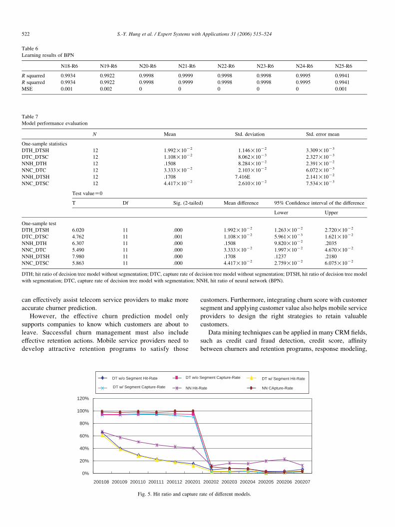
Table 6

Learning results of BPN

N18-R6 N19-R6 N20-R6 N21-R6 N22-R6 N23-R6 N24-R6 N25-R6

R squarred 0.9934 0.9922 0.9998 0.9999 0.9998 0.9998 0.9995 0.9941

R squarred 0.9934 0.9922 0.9998 0.9999 0.9998 0.9998 0.9995 0.9941

MSE 0.001 0.002 0 0 0 0 0 0.001

Table 7

Model performance evaluation

N Mean Std. deviation Std. error mean

One-sample statistics

DTH_DTSH 12 1.992!10K2 1.146!10K2 3.309!10K3

DTC_DTSC 12 1.108!10K2 8.062!10K3 2.327!10K3

NNH_DTH 12 .1508 8.284!10K2 2.391!10K2

NNC_DTC 12 3.333!10K2 2.103!10K2 6.072!10K3

NNH_DTSH 12 .1708 7.416E 2.141!10K2

NNC_DTSC 12 4.417!10K2 2.610!10K2 7.534!10K3

Test valueZ0

T Df Sig. (2-tailed) Mean difference 95% Confidence interval of the difference

Lower Upper

One-sample test

DTH_DTSH 6.020 11 .000 1.992!10K2 1.263!10K2 2.720!10K2

DTC_DTSC 4.762 11 .001 1.108!10K2 5.961!10K3 1.621!10K2

NNH_DTH 6.307 11 .000 .1508 9.820!10K2 .2035

NNC_DTC 5.490 11 .000 3.333!10K2 1.997!10K2 4.670!10K2

NNH_DTSH 7.980 11 .000 .1708 .1237 .2180

NNC_DTSC 5.863 11 .000 4.417!10K2 2.759!10K2 6.075!10K2

DTH; hit ratio of decision tree model without segmentation; DTC, capture rate of decision tree model without segmentation; DTSH, hit ratio of decision tree model

with segmentation; DTC, capture rate of decision tree model with segmentation; NNH, hit ratio of neural network (BPN).


can effectively assist telecom service providers to make more

accurate churner prediction.

However, the effective churn prediction model only

supports companies to know which customers are about to

leave. Successful churn management must also include

effective retention actions. Mobile service providers need to

develop attractive retention programs to satisfy those

0%

20%

40%

60%

80%

100%

120%

200108 200109 200110 200111 200112 200201

DT w/o Segment Hit-Rate DT w/o

DT w/ Segment Capture-Rate NN Hit-

Fig. 5. Hit ratio and capture

customers. Furthermore, integrating churn score with customer

segment and applying customer value also helps mobile service

providers to design the right strategies to retain valuable

customers.

Data mining techniques can be applied in many CRM fields,

such as credit card fraud detection, credit score, affinity

between churners and retention programs, response modeling,

200202 200203 200204 200205 200206 200207

Segment Capture-Rate DT w/ Segment Hit-Rate

Rate NN CApture-Rate

rate of different models.

0%

20%

40%

60%

80%

100%

120%

200108 200109 200110 200111 200112 200201 200202 200203 200204 200205 200206 200207

Validation Month (YYYYMM)

Rat

e

DT w/o Segment Hit-Rate DT w/o Segment Capture-Rate DT w/ Segment Hit-Rate

DT w/ Segment Capture-Rate NN Hit-Rate NN Capture-Rate

Fig. 6. Model performance with 50,000 subscribers.

Neural Network

0

5

10

15

20

25

30

0% 10% 20% 30% 40% 50% 60% 70% 80% 90% 100%

% of Population

Lift

DT W/O Segment

05

101520253035

0% 10% 20% 30% 40% 50% 60% 70% 80% 90% 100%

% of Population

Lift

DT With Segment

0

5

10

15

20

25

30

0% 10% 20% 30% 40% 50% 60% 70% 80% 90% 100%

% of Population

Lift

Fig. 7. LIFT comparison.


and customer purchase decision modeling. We expect to see

more data mining applications in business management, and

more sophisticated data mining techniques will be developed

as business complexity increases.

References

Berson, A., Smith, S., & Thearling, K. (2000). Building data mining

applications for CRM. New York, NY: McGraw-Hill.

Bortiz, J. E., & Kennedy, D. B. (1995). Effectiveness of neural network types

for prediction of business failure. Expert Systems with Applications, 9(4),

503–512.

Cybenco, H. (1998). Approximation by super-positions of sigmoidal function.

Mathematical Control Cignal Systems, 2, 303–314.

Fletcher, D., & Goss, E. (1993). Forecasting with neural networks: An

application using bankruptcy data. Information and Management, 3,

159–167.

Kentrias, S. (2001). Customer relationship management: The SAS perspective,

www.cm2day.com.

Langley, P., & Simon, H. A. (1995). Applications of machine learning and rule

induction. Communication of the ACM, 38(11), 55–64.

Lariviere, B., Van den Poel, D., & Van den Poel (2004). Investigating the role

of product features in preventing customer churn, by using survival analysis

and choice modeling: The case of financial services. Expert Systems with

Applications, 27(2), 277–285.

Lau, H. C. W., Wong, C. W. Y., Hui, I. K., & Pun, K. F. (2003). Design and

implementation of an integrated knowledge system. Knowledge-Based

Systems, 16(2), 69–76.

Lejeune, M. (2001). Measuring the impact of data mining on churn

management. Internet Research: Electronic Network Applications and

Policy, 11(5), 375–387.

Mattersion, R. (2001). Telecom churn management. Fuquay-Varina, NC:

APDG Publishing.

Salchenberger, L. M., Cinar, E. M., & Lash, N. A. (1992). Neural networks: A

new tool for predicting thrift failures. Decision Sciences, 23(4), 899–916.

http://www.cm2day.com


SAS Institute, (2000). Best Price in Churn Prediction, SAS Institute White

Paper.

Su, C. T., Hsu, H. H., & Tsai, C. H. (2002). Knowledge mining from trained

neural networks. Journal of Computer Information Systems, 42(4), 61–70.

Tam, K. Y., & Kiang, M. Y. (1992). Managerial applications of neural

networks: The case of bank failure predictions. Management Science,

38(7), 926–947.

Thearling, K. (1999). An introduction of data mining. Direct Marketing

Magazine .

Wei, C. P., & Chiu, I. T. (2002). Tuning telecommunications call detail to

churn prediction: A data mining approach. Expert Systems with

Applications, 23, 103–112.

Zhan, G., Patuwo, B. E., & Hu, M. Y. (1998). Forecasting with artificial neural

network: The state of the art. International Journal of Forecasting, 14, 35–62.

Zhang, G., Hu, M. Y., Patuwo, B. E., & Indro, D. C. (1999). Artificial neural

networks in bankruptcy prediction: General framework and cross-

validation analysis. European Journal of Operational Research, 116,

16–32.

Documents

Applying data mining to telecom churn management