Embed Size (px)
Citation preview
Applying the Boundary-Layer IndependencePrinciple to Turbulent Flows
Israel Wygnanski,∗ Philipp Tewes,† and Lutz Taubert‡
University of Arizona, Tucson, Arizona 85721
DOI: 10.2514/1.C032206
Velocities measured in turbulent boundary layers over yawed flat plates confirmed that the mean velocity profiles
normal to the leading edge are proportional to the velocity profiles parallel to it, with a proportionality constant
depending on the yaw angle. This turned out to be the necessary and sufficient condition to make the wall stress
components normal and parallel to the leading edge also proportional in the same manner, thus reaffirming the
boundary-layer independence principle for turbulent and laminar flows alike. Reinterpretation of old experiments
thus changed themantra stating, “the independence principle does not apply to turbulent flow”, thus providing a new
insight into three-dimensional boundary-layer flows on yawed, high-aspect-ratio wings. It explains the prevalence of
attached spanwise flow near the trailing edges of such wings, and it provides a rationale for turbulence modeling on
them. Furthermore, it indicates the direction along which active separation control should take place.
Nomenclature
CD = sectional/wing-drag coefficientCL = sectional/wing-lift coefficientCf = skin-friction coefficientCp = pressure coefficientCμ = momentum coefficientc = chord normal to leading edgecξ = chord in freestream directionD = drag forceG = function describing skin friction of y∕δH = boundary-layer shape parameterk, κ = constantsMa = Mach numberp = static pressureRe = Reynolds numberUe, Ve,We = velocities at the edge of the boundary layer in x, y,
and z directionsUτ, Vτ, Wτ = friction velocities in x, y, and z directionsU∞ = freestream velocityu�, y� = dimensionless velocity, dimensionless wall
coordinateu, v, w = velocities inside the boundary layer in x, y, and z
directionsx, y, z = body-fixed coordinate systemξ, y, ζ = coordinate system in direction of streamα = angle of attackδ = boundary-layer thicknessδf = flap deflectionδ� = displacement thicknessη = self-similarity coordinateΛ = yaw angleθ = momentum thicknessμ = dynamic viscosityν = kinematic viscosityρ = air density
τ = total shear stressΦ = flow angle on surfaceΨ = stream function
Introduction
R ECENT observations in a turbulent mixing layer emanatingfrom a skewed trailing edge indicated that the boundary-layer
equations governing the evolution of this flow in the direction normalto the trailing edge are independent of the equations governing thespanwise flow along it [1]. Thus, the applicability of the indepen-dence principle to this highly turbulent flow triggered a renewedinterest in the old measurements (e.g., [2,3]) that refuted its validityto turbulent boundary layers thus changing the mantra “theindependence principle does not apply to turbulent flow” [4].The boundary-layer equations representing incompressible flow
over a yawed flat plate are
∂u∕∂x� ∂v∕∂y � 0 (1)
ρ�∂�uu�∕∂x� ∂�vu�∕∂y� � ∂τxy∕∂y (2)
ρ�∂�uw�∕∂x� ∂�vw�∕∂y� � ∂τzy∕∂y (3)
Where u and w are components of velocity in the directions normal(x), and parallel (z) to the leading edge of the plate, thus at y→∞: u → Ue � U∞ cos Λ andw → We � U∞ sin ΛwhereΛ is theyaw angle (Fig. 1). All of the derivatives ∂∕∂z � 0 due the infiniteaspect ratio of the yawed plate. The somewhat unusual representationof the momentum equations results from the addition of the conti-nuity equation to the equations of momentum after multiplying it bythe appropriate velocity component.In laminar flow, τxy � μ∂u∕∂y and τzy � μ∂w∕∂y; thus, the two
momentum equations are identical, as are their respective boundaryconditions. Therefore, the solutions are proportional to one anotherwith the proportionality constant depending on Λ. Each one of themomentum equations provides a balance between the inertia termsand the stress terms; thus, knowledge of one determines the other andvice versa, regardless of the state of the flow. Hence, if in turbulentflow, u�x; y� is proportional to w�x; y�, the shear stresses should beproportional to one another as well (i.e., τxy ∝ τzy, and this includesthe different Reynolds stress terms as well, and in particular, ρu 0v 0 ∝ρw 0v 0 because these are the dominant terms outside the viscoussublayer). It permits one to solve Eqs. (1) and (2) independently ofEq. (3) because the two first equations do not contain w terms. Thistype of boundary-layer solutions is referred to in the literature as the
Received 26 November 2012; revision received 1 July 2013; accepted forpublication 10 July 2013; published online 24 January 2014. Copyright ©2013 by the American Institute of Aeronautics and Astronautics, Inc. Allrights reserved. Copies of this paper may be made for personal or internal use,on condition that the copier pay the $10.00 per-copy fee to the CopyrightClearance Center, Inc., 222 Rosewood Drive, Danvers, MA 01923; includethe code 1542-3868/14 and $10.00 in correspondence with the CCC.
*Professor, Department ofAerospace andMechanical Engineering. FellowAIAA.
†Research Associate, Department of Aerospace and MechanicalEngineering. Student Member AIAA.
‡Research Assistant Professor, Department of Aerospace and MechanicalEngineering. Member AIAA.
175
JOURNAL OF AIRCRAFT
Vol. 51, No. 1, January–February 2014
Dow
nloa
ded
by C
AR
LE
TO
N U
NIV
ER
SIT
Y L
IBR
AR
Y o
n Ju
ly 3
, 201
4 | h
ttp://
arc.
aiaa
.org
| D
OI:
10.
2514
/1.C
0322
06
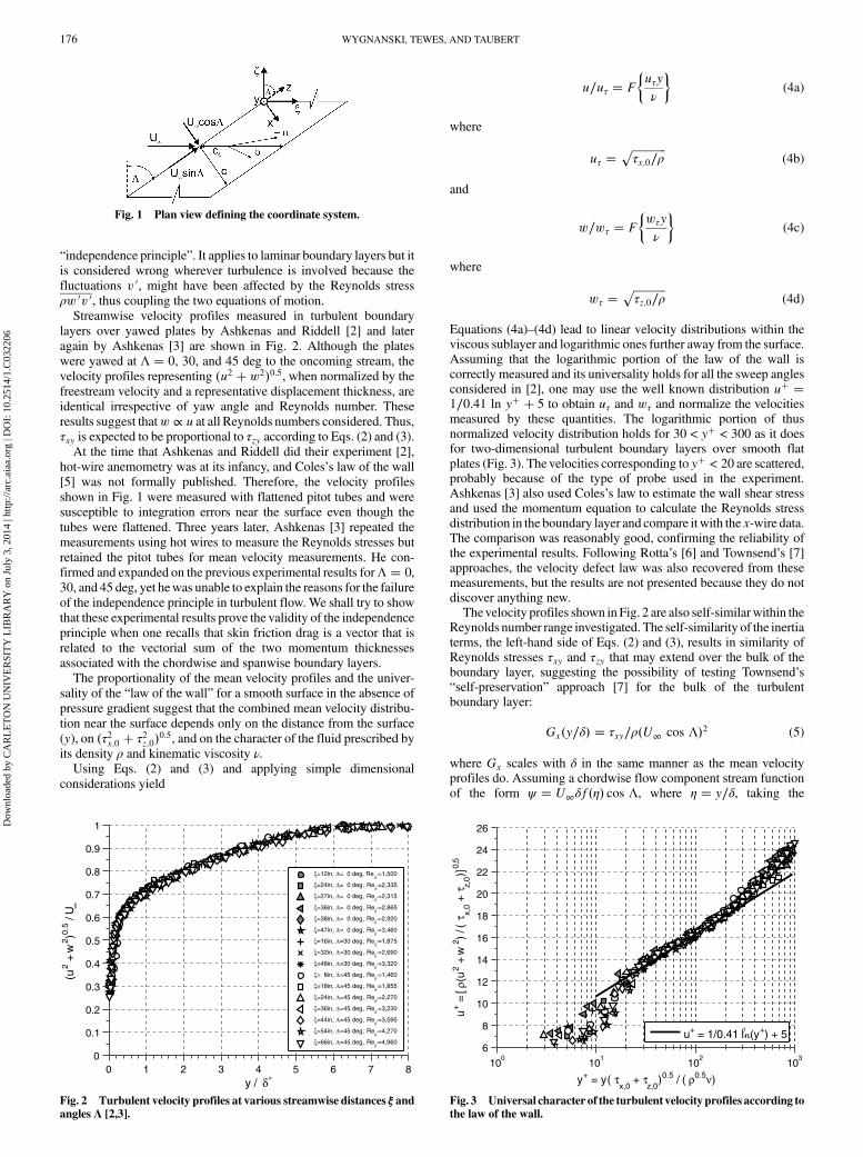
“independence principle”. It applies to laminar boundary layers but itis considered wrong wherever turbulence is involved because thefluctuations v 0, might have been affected by the Reynolds stressρw 0v 0, thus coupling the two equations of motion.Streamwise velocity profiles measured in turbulent boundary
layers over yawed plates by Ashkenas and Riddell [2] and lateragain by Ashkenas [3] are shown in Fig. 2. Although the plateswere yawed at Λ � 0, 30, and 45 deg to the oncoming stream, thevelocity profiles representing �u2 �w2�0.5, when normalized by thefreestream velocity and a representative displacement thickness, areidentical irrespective of yaw angle and Reynolds number. Theseresults suggest thatw ∝ u at all Reynolds numbers considered. Thus,τxy is expected to be proportional to τzy according to Eqs. (2) and (3).At the time that Ashkenas and Riddell did their experiment [2],
hot-wire anemometry was at its infancy, and Coles’s law of the wall[5] was not formally published. Therefore, the velocity profilesshown in Fig. 1 were measured with flattened pitot tubes and weresusceptible to integration errors near the surface even though thetubes were flattened. Three years later, Ashkenas [3] repeated themeasurements using hot wires to measure the Reynolds stresses butretained the pitot tubes for mean velocity measurements. He con-firmed and expanded on the previous experimental results forΛ � 0,30, and 45 deg, yet hewas unable to explain the reasons for the failureof the independence principle in turbulent flow. We shall try to showthat these experimental results prove the validity of the independenceprinciple when one recalls that skin friction drag is a vector that isrelated to the vectorial sum of the two momentum thicknessesassociated with the chordwise and spanwise boundary layers.The proportionality of the mean velocity profiles and the univer-
sality of the “law of the wall” for a smooth surface in the absence ofpressure gradient suggest that the combined mean velocity distribu-tion near the surface depends only on the distance from the surface(y), on �τ2x;0 � τ2z;0�0.5, and on the character of the fluid prescribed byits density ρ and kinematic viscosity ν.Using Eqs. (2) and (3) and applying simple dimensional
considerations yield
u∕uτ � F�uτy
ν
�(4a)
where
uτ ��������������τx;0∕ρ
p(4b)
and
w∕wτ � F�wτy
ν
�(4c)
where
wτ �������������τz;0∕ρ
p(4d)
Equations (4a)–(4d) lead to linear velocity distributions within theviscous sublayer and logarithmic ones further away from the surface.Assuming that the logarithmic portion of the law of the wall iscorrectly measured and its universality holds for all the sweep anglesconsidered in [2], one may use the well known distribution u� �1∕0.41 ln y� � 5 to obtain uτ and wτ and normalize the velocitiesmeasured by these quantities. The logarithmic portion of thusnormalized velocity distribution holds for 30 < y� < 300 as it doesfor two-dimensional turbulent boundary layers over smooth flatplates (Fig. 3). The velocities corresponding to y� < 20 are scattered,probably because of the type of probe used in the experiment.Ashkenas [3] also used Coles’s law to estimate the wall shear stressand used the momentum equation to calculate the Reynolds stressdistribution in the boundary layer and compare it with the x-wire data.The comparison was reasonably good, confirming the reliability ofthe experimental results. Following Rotta’s [6] and Townsend’s [7]approaches, the velocity defect law was also recovered from thesemeasurements, but the results are not presented because they do notdiscover anything new.Thevelocity profiles shown in Fig. 2 are also self-similarwithin the
Reynolds number range investigated. The self-similarity of the inertiaterms, the left-hand side of Eqs. (2) and (3), results in similarity ofReynolds stresses τxy and τzy that may extend over the bulk of theboundary layer, suggesting the possibility of testing Townsend’s“self-preservation” approach [7] for the bulk of the turbulentboundary layer:
Gx�y∕δ� � τxy∕ρ�U∞ cos Λ�2 (5)
where Gx scales with δ in the same manner as the mean velocityprofiles do. Assuming a chordwise flow component stream functionof the form ψ � U∞δf�η� cos Λ, where η � y∕δ, taking the
Fig. 1 Plan view defining the coordinate system.
0 1 2 3 4 5 6 7 80
0.1
0.2
0.3
0.4
0.5
0.6
0.7
0.8
0.9
1
y / δ∗
(u2 +
w2 )0.
5 / U ∞
ξ=12in, Λ= 0 deg, Reδ
∗=1,500
ξ=24in, Λ= 0 deg, Reδ
∗=2,335
ξ=27in, Λ= 0 deg, Reδ
∗=2,315
ξ=36in, Λ= 0 deg, Reδ
∗=2,865
ξ=38in, Λ= 0 deg, Reδ
∗=2,920
ξ=47in, Λ= 0 deg, Reδ
∗=3,460
ξ=16in, Λ=30 deg, Reδ
∗=1,875
ξ=32in, Λ=30 deg, Reδ
∗=2,690
ξ=48in, Λ=30 deg, Reδ
∗=3,320
ξ= 8in, Λ=45 deg, Reδ
∗=1,460
ξ=18in, Λ=45 deg, Reδ
∗=1,855
ξ=24in, Λ=45 deg, Reδ
∗=2,270
ξ=36in, Λ=45 deg, Reδ
∗=3,230
ξ=44in, Λ=45 deg, Reδ
∗=3,595
ξ=54in, Λ=45 deg, Reδ
∗=4,270
ξ=66in, Λ=45 deg, Reδ
∗=4,960
Fig. 2 Turbulent velocity profiles at various streamwise distances ξ andangles Λ [2,3].
100
101
102
103
6
8
10
12
14
16
18
20
22
24
26
y+ = y ( τx,0
+ τz,0
)0.5 / ( ρ0.5ν)
u+ =
[ρ(
u2 +
w2 )
/ (τ x,
0 + τ z,
0)]
0.5
u+ = 1/0.41 (y+) + 5
Fig. 3 Universal character of the turbulent velocity profiles according tothe law of the wall.
176 WYGNANSKI, TEWES, AND TAUBERT
Dow
nloa
ded
by C
AR
LE
TO
N U
NIV
ER
SIT
Y L
IBR
AR
Y o
n Ju
ly 3
, 201
4 | h
ttp://
arc.
aiaa
.org
| D
OI:
10.
2514
/1.C
0322
06
appropriate derivatives and substituting them in Eq. (2) together withGx results in
G 0x � �dδ∕dx�ff 0 0 � 0 (6)
For self-similarity to exist, Eq. (6) will have to depend only on asingle variable (η), and dδ∕dx needs to be constant, suggestingthat δ � κx � κξ cos Λ.The boundary-layer thicknesses reported in [2,3,8] were all
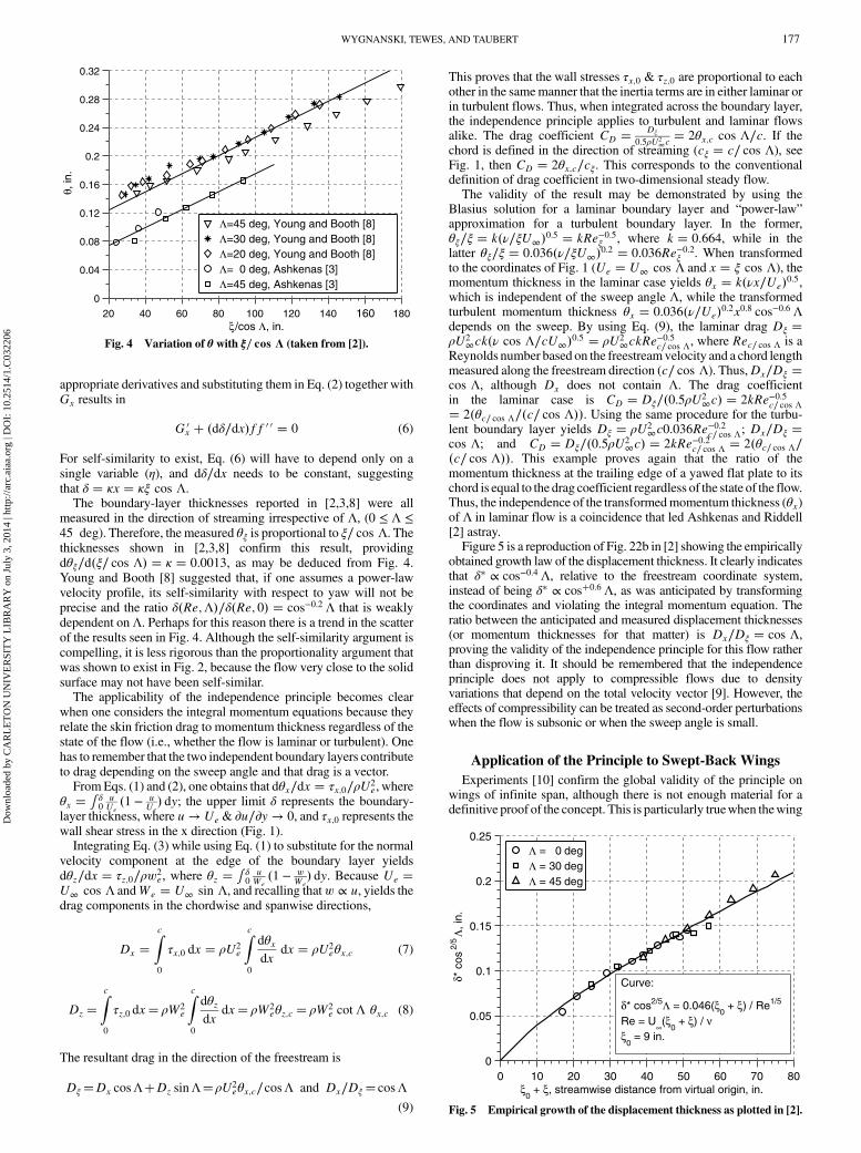
measured in the direction of streaming irrespective of Λ, (0 ≤ Λ ≤45 deg). Therefore, the measured θξ is proportional to ξ∕ cos Λ. Thethicknesses shown in [2,3,8] confirm this result, providingdθξ∕d�ξ∕ cos Λ� � κ � 0.0013, as may be deduced from Fig. 4.Young and Booth [8] suggested that, if one assumes a power-lawvelocity profile, its self-similarity with respect to yaw will not beprecise and the ratio δ�Re;Λ�∕δ�Re; 0� � cos−0.2 Λ that is weaklydependent on Λ. Perhaps for this reason there is a trend in the scatterof the results seen in Fig. 4. Although the self-similarity argument iscompelling, it is less rigorous than the proportionality argument thatwas shown to exist in Fig. 2, because the flow very close to the solidsurface may not have been self-similar.The applicability of the independence principle becomes clear
when one considers the integral momentum equations because theyrelate the skin friction drag to momentum thickness regardless of thestate of the flow (i.e., whether the flow is laminar or turbulent). Onehas to remember that the two independent boundary layers contributeto drag depending on the sweep angle and that drag is a vector.FromEqs. (1) and (2), one obtains that dθx∕dx � τx;0∕ρU2
e, whereθx � ∫ δ
0uUe�1 − u
Ue� dy; the upper limit δ represents the boundary-
layer thickness, where u → Ue & ∂u∕∂y→ 0, and τx;0 represents thewall shear stress in the x direction (Fig. 1).Integrating Eq. (3) while using Eq. (1) to substitute for the normal
velocity component at the edge of the boundary layer yieldsdθz∕dx � τz;0∕ρw2
e, where θz � ∫ δ0uWe�1 − w
We� dy. Because Ue �
U∞ cos Λ andWe � U∞ sin Λ, and recalling thatw ∝ u, yields thedrag components in the chordwise and spanwise directions,
Dx �Zc
0
τx;0 dx � ρU2e
Zc
0
dθxdx
dx � ρU2eθx;c (7)
Dz�Zc
0
τz;0 dx� ρW2e
Zc
0
dθzdx
dx� ρW2eθz;c� ρW2
e cot Λ θx;c (8)
The resultant drag in the direction of the freestream is
Dξ�Dx cosΛ�Dz sinΛ�ρU2eθx;c∕cosΛ and Dx∕Dξ�cosΛ
(9)
This proves that the wall stresses τx;0 & τz;0 are proportional to eachother in the samemanner that the inertia terms are in either laminar orin turbulent flows. Thus, when integrated across the boundary layer,the independence principle applies to turbulent and laminar flowsalike. The drag coefficient CD �
Dξ
0.5ρU2∞c� 2θx;c cos Λ∕c. If the
chord is defined in the direction of streaming (cξ � c∕ cos Λ), seeFig. 1, then CD � 2θx;c∕cξ. This corresponds to the conventionaldefinition of drag coefficient in two-dimensional steady flow.The validity of the result may be demonstrated by using the
Blasius solution for a laminar boundary layer and “power-law”approximation for a turbulent boundary layer. In the former,θξ∕ξ � k�ν∕ξU∞�0.5 � kRe−0.5ξ , where k � 0.664, while in thelatter θξ∕ξ � 0.036�ν∕ξU∞�0.2 � 0.036Re−0.2ξ . When transformedto the coordinates of Fig. 1 (Ue � U∞ cos Λ and x � ξ cos Λ), themomentum thickness in the laminar case yields θx � k�νx∕Ue�0.5,which is independent of the sweep angle Λ, while the transformedturbulent momentum thickness θx � 0.036�ν∕Ue�0.2x0.8 cos−0.6 Λdepends on the sweep. By using Eq. (9), the laminar drag Dξ �ρU2
∞ck�ν cos Λ∕cU∞�0.5 � ρU2∞ckRe
−0.5c∕ cos Λ, where Rec∕ cos Λ is a
Reynolds number based on the freestreamvelocity and a chord lengthmeasured along the freestream direction (c∕ cos Λ). Thus,Dx∕Dξ �cos Λ, although Dx does not contain Λ. The drag coefficientin the laminar case is CD � Dξ∕�0.5ρU2
∞c� � 2kRe−0.5c∕ cos Λ� 2�θc∕ cos Λ∕�c∕ cos Λ��. Using the same procedure for the turbu-lent boundary layer yields Dξ � ρU2
∞c0.036Re−0.2c∕ cos Λ; Dx∕Dξ �
cos Λ; and CD � Dξ∕�0.5ρU2∞c� � 2kRe−0.2c∕ cos Λ � 2�θc∕ cos Λ∕
�c∕ cos Λ��. This example proves again that the ratio of themomentum thickness at the trailing edge of a yawed flat plate to itschord is equal to the drag coefficient regardless of the state of the flow.Thus, the independence of the transformedmomentum thickness (θx)of Λ in laminar flow is a coincidence that led Ashkenas and Riddell[2] astray.Figure 5 is a reproduction of Fig. 22b in [2] showing the empirically
obtained growth law of the displacement thickness. It clearly indicatesthat δ� ∝ cos−0.4 Λ, relative to the freestream coordinate system,instead of being δ� ∝ cos�0.6 Λ, as was anticipated by transformingthe coordinates and violating the integral momentum equation. Theratio between the anticipated and measured displacement thicknesses(or momentum thicknesses for that matter) is Dx∕Dξ � cos Λ,proving the validity of the independence principle for this flow ratherthan disproving it. It should be remembered that the independenceprinciple does not apply to compressible flows due to densityvariations that depend on the total velocity vector [9]. However, theeffects of compressibility can be treated as second-order perturbationswhen the flow is subsonic or when the sweep angle is small.
Application of the Principle to Swept-Back Wings
Experiments [10] confirm the global validity of the principle onwings of infinite span, although there is not enough material for adefinitive proof of the concept. This is particularly truewhen thewing
20 40 60 80 100 120 140 160 180
0
0.04
0.08
0.12
0.16
0.2
0.24
0.28
0.32
ξ/cos Λ, in.
θ, in
.
Λ=45 deg, Young and Booth [8]Λ=30 deg, Young and Booth [8]Λ=20 deg, Young and Booth [8]Λ= 0 deg, Ashkenas [3]Λ=45 deg, Ashkenas [3]
Fig. 4 Variation of θ with ξ∕ cos Λ (taken from [2]).
0 10 20 30 40 50 60 70 800
0.05
0.1
0.15
0.2
0.25
ξ0 + ξ, streamwise distance from virtual origin, in.
δ* c
os2/
5Λ
, in.
Λ = 0 degΛ = 30 degΛ = 45 deg
Curve:
δ* cos2/5Λ = 0.046(ξ0 + ξ) / Re1/5
Re = U∞(ξ
0 + ξ) / ν
ξ0 = 9 in.
Fig. 5 Empirical growth of the displacement thickness as plotted in [2].
WYGNANSKI, TEWES, AND TAUBERT 177
Dow
nloa
ded
by C
AR
LE
TO
N U
NIV
ER
SIT
Y L
IBR
AR
Y o
n Ju
ly 3
, 201
4 | h
ttp://
arc.
aiaa
.org
| D
OI:
10.
2514
/1.C
0322
06
is lifting and the numerical solution depends on the turbulence modelused. In this case, themomentum equation normal to the leading edgecontains a pressure gradient term:
ρ�∂�uu�∕∂x� ∂�vu�∕∂y� � −dp∕dx� ∂τxy∕∂y (10)
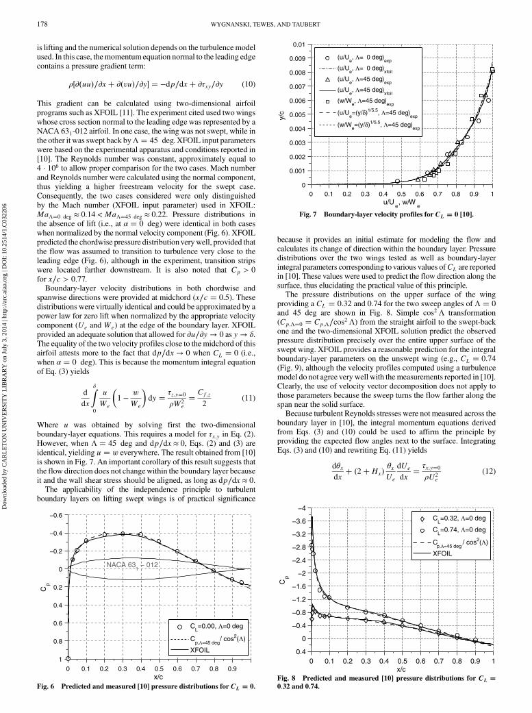
This gradient can be calculated using two-dimensional airfoilprograms such as XFOIL [11]. The experiment cited used twowingswhose cross section normal to the leading edge was represented by aNACA 631-012 airfoil. In one case, the wing was not swept, while inthe other it was swept back byΛ � 45 deg. XFOIL input parameterswere based on the experimental apparatus and conditions reported in[10]. The Reynolds number was constant, approximately equal to4 · 106 to allow proper comparison for the two cases. Mach numberand Reynolds number were calculated using the normal component,thus yielding a higher freestream velocity for the swept case.Consequently, the two cases considered were only distinguishedby the Mach number (XFOIL input parameter) used in XFOIL:MaΛ�0 deg ≈ 0.14 < MaΛ�45 deg ≈ 0.22. Pressure distributions inthe absence of lift (i.e., at α � 0 deg) were identical in both caseswhen normalized by the normal velocity component (Fig. 6). XFOILpredicted the chordwise pressure distributionverywell, provided thatthe flow was assumed to transition to turbulence very close to theleading edge (Fig. 6), although in the experiment, transition stripswere located farther downstream. It is also noted that Cp > 0for x∕c > 0.77.Boundary-layer velocity distributions in both chordwise and
spanwise directions were provided at midchord (x∕c � 0.5). Thesedistributions were virtually identical and could be approximated by apower law for zero lift when normalized by the appropriate velocitycomponent (Ue and We) at the edge of the boundary layer. XFOILprovided an adequate solution that allowed for ∂u∕∂y → 0 as y → δ.The equality of the two velocity profiles close to the midchord of thisairfoil attests more to the fact that dp∕dx→ 0 when CL � 0 (i.e.,when α � 0 deg). This is because the momentum integral equationof Eq. (3) yields
d
dx
Zδ
0
u
We
�1 −
w
We
�dy �
τz;y�0ρW2
e
�Cf;z2
(11)
Where u was obtained by solving first the two-dimensionalboundary-layer equations. This requires a model for τx;y in Eq. (2).However, when Λ � 45 deg and dp∕dx ≈ 0, Eqs. (2) and (3) areidentical, yielding u � w everywhere. The result obtained from [10]is shown in Fig. 7. An important corollary of this result suggests thatthe flow direction does not changewithin the boundary layer becauseit and the wall shear stress should be aligned, as long as dp∕dx ≈ 0.The applicability of the independence principle to turbulent
boundary layers on lifting swept wings is of practical significance
because it provides an initial estimate for modeling the flow andcalculates its change of direction within the boundary layer. Pressuredistributions over the two wings tested as well as boundary-layerintegral parameters corresponding to various values ofCL are reportedin [10]. These values were used to predict the flow direction along thesurface, thus elucidating the practical value of this principle.The pressure distributions on the upper surface of the wing
providing a CL � 0.32 and 0.74 for the two sweep angles of Λ � 0and 45 deg are shown in Fig. 8. Simple cos2 Λ transformation(Cp;Λ�0 � Cp;Λ∕cos2 Λ) from the straight airfoil to the swept-backone and the two-dimensional XFOIL solution predict the observedpressure distribution precisely over the entire upper surface of theswept wing. XFOIL provides a reasonable prediction for the integralboundary-layer parameters on the unswept wing (e.g., CL � 0.74(Fig. 9), although the velocity profiles computed using a turbulencemodel do not agree very well with themeasurements reported in [10].Clearly, the use of velocity vector decomposition does not apply tothose parameters because the sweep turns the flow farther along thespan near the solid surface.Because turbulent Reynolds stresses were not measured across the
boundary layer in [10], the integral momentum equations derivedfrom Eqs. (3) and (10) could be used to affirm the principle byproviding the expected flow angles next to the surface. IntegratingEqs. (3) and (10) and rewriting Eq. (11) yields
dθxdx� �2�Hx�
θxUe
dUedx�
τx;y�0ρU2
e
(12)
0 0.1 0.2 0.3 0.4 0.5 0.6 0.7 0.8 0.9
−0.6
−0.4
−0.2
0
0.2
0.4
0.6
0.8
1
NACA 631 − 012
x/c
Cp
CL=0.00, Λ=0 deg
Cp,Λ=45 deg
/ cos2(Λ)
XFOIL
Fig. 6 Predicted and measured [10] pressure distributions for CL � 0.
0 0.1 0.2 0.3 0.4 0.5 0.6 0.7 0.8 0.9 10
0.001
0.002
0.003
0.004
0.005
0.006
0.007
0.008
0.009
0.01
u/Ue, w/W
e
y/c
(u/Ue, Λ= 0 deg)
exp
(u/Ue, Λ= 0 deg)
xfoil
(u/Ue, Λ=45 deg)
exp
(u/Ue, Λ=45 deg)
xfoil
(w/We, Λ=45 deg)
exp
(u/Ue=(y/δ)1/5.5, Λ=45 deg)
exp
(w/We=(y/δ)1/5.5, Λ=45 deg)
exp
Fig. 7 Boundary-layer velocity profiles for CL � 0 [10].
0 0.1 0.2 0.3 0.4 0.5 0.6 0.7 0.8 0.9 1
−4
−3.6
−3.2
−2.8
−2.4
−2
−1.6
−1.2
−0.8
−0.4
0
0.4
x/c
Cp
CL=0.32, Λ=0 deg
CL=0.74, Λ=0 deg
Cp,Λ=45 deg
/ cos2(Λ)
XFOIL
Fig. 8 Predicted and measured [10] pressure distributions for CL �0.32 and 0.74.
178 WYGNANSKI, TEWES, AND TAUBERT
Dow
nloa
ded
by C
AR
LE
TO
N U
NIV
ER
SIT
Y L
IBR
AR
Y o
n Ju
ly 3
, 201
4 | h
ttp://
arc.
aiaa
.org
| D
OI:
10.
2514
/1.C
0322
06
and dθz∕dx � τz;y�0∕ρW2e with We � U∞ sin Λ (no spanwise
pressure gradient)Thus, the flow angle for y → 0 can be estimated using
ϕ � tan−1�τz;y�0∕τx;y�0� − Λ (13)
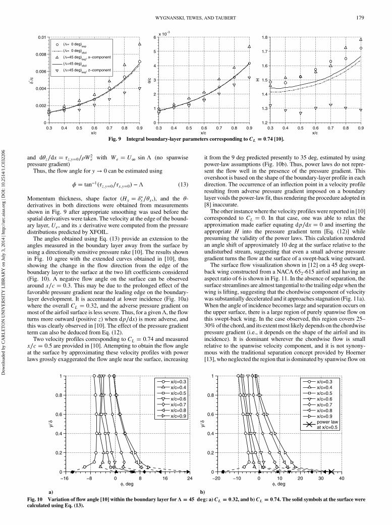
Momentum thickness, shape factor (Hx � δ�x∕θx,), and the θ-derivatives in both directions were obtained from measurementsshown in Fig. 9 after appropriate smoothing was used before thespatial derivatives were taken. The velocity at the edge of the bound-ary layer, Ue, and its x derivative were computed from the pressuredistributions predicted by XFOIL.The angles obtained using Eq. (13) provide an extension to the
angles measured in the boundary layer away from the surface byusing a directionally sensitive pressure rake [10]. The results shownin Fig. 10 agree with the extended curves obtained in [10], thusshowing the change in the flow direction from the edge of theboundary layer to the surface at the two lift coefficients considered(Fig. 10). A negative flow angle on the surface can be observedaround x∕c � 0.3. This may be due to the prolonged effect of thefavorable pressure gradient near the leading edge on the boundary-layer development. It is accentuated at lower incidence (Fig. 10a)where the overall CL � 0.32, and the adverse pressure gradient onmost of the airfoil surface is less severe. Thus, for a givenΛ, the flowturns more outward (positive z) when dp∕dx) is more adverse, andthis was clearly observed in [10]. The effect of the pressure gradientterm can also be deduced from Eq. (12).Two velocity profiles corresponding to CL � 0.74 and measured
x∕c � 0.5 are provided in [10]. Attempting to obtain the flow angleat the surface by approximating these velocity profiles with powerlaws grossly exaggerated the flow angle near the surface, increasing
it from the 9 deg predicted presently to 35 deg, estimated by usingpower-law assumptions (Fig. 10b). Thus, power laws do not repre-sent the flow well in the presence of the pressure gradient. Thisovershoot is based on the shape of the boundary-layer profile in eachdirection. The occurrence of an inflection point in a velocity profileresulting from adverse pressure gradient imposed on a boundarylayer voids the power-law fit, thus rendering the procedure adopted in[8] inaccurate.The other instancewhere the velocity profileswere reported in [10]
corresponded to CL � 0. In that case, one was able to relax theapproximation made earlier equating dp∕dx � 0 and inserting theappropriate H into the pressure gradient term [Eq. (12)] whilepresuming the validity of the power laws. This calculation renderedan angle shift of approximately 10 deg at the surface relative to theundisturbed stream, suggesting that even a small adverse pressuregradient turns the flow at the surface of a swept-back wing outward.The surface flow visualization shown in [12] on a 45 deg swept-
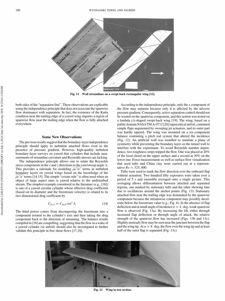
back wing constructed from a NACA 652-615 airfoil and having anaspect ratio of 6 is shown in Fig. 11. In the absence of separation, thesurface streamlines are almost tangential to the trailing edgewhen thewing is lifting, suggesting that the chordwise component of velocitywas substantially decelerated and it approaches stagnation (Fig. 11a).When the angle of incidence becomes large and separation occurs onthe upper surface, there is a large region of purely spanwise flow onthis swept-back wing. In the case observed, this region covers 25–30%of the chord, and its extentmost likely depends on the chordwisepressure gradient (i.e., it depends on the shape of the airfoil and itsincidence). It is dominant wherever the chordwise flow is smallrelative to the spanwise velocity component, and it is not synony-mous with the traditional separation concept provided by Hoerner[13], who neglected the region that is dominated by spanwise flow on
0.3 0.4 0.5 0.6 0.7 0.8 0.90
0.002
0.004
0.006
0.008
0.01
x/c
δ* /c
0.3 0.4 0.5 0.6 0.7 0.8 0.90
1
2
3
4
5
6x 10
−3
x/c
θ/c
0.3 0.4 0.5 0.6 0.7 0.8 0.91.2
1.3
1.4
1.5
1.6
1.7
1.8
x/c
H
(Λ= 0 deg)exp
(Λ= 0 deg)xfoil
(Λ=45 deg)exp
, x−component
(Λ=45 deg)xfoil
(Λ=45 deg)exp
, z−component
Fig. 9 Integral boundary-layer parameters corresponding to CL � 0.74 [10].
−16 −8 0 8 16 240
0.2
0.4
0.6
0.8
1
φ, deg
y/δ
x/c=0.3x/c=0.4x/c=0.5x/c=0.6x/c=0.7x/c=0.8x/c=0.9
−20 −10 0 10 20 30 400
0.2
0.4
0.6
0.8
1
φ, deg
y/δ
x/c=0.3x/c=0.4x/c=0.5x/c=0.6x/c=0.7x/c=0.8x/c=0.9power lawat x/c=0.5
a) b)Fig. 10 Variation of flow angle [10] within the boundary layer for Λ � 45 deg: a) CL � 0.32, and b) CL � 0.74. The solid symbols at the surface werecalculated using Eq. (13).
WYGNANSKI, TEWES, AND TAUBERT 179
Dow
nloa
ded
by C
AR
LE
TO
N U
NIV
ER
SIT
Y L
IBR
AR
Y o
n Ju
ly 3
, 201
4 | h
ttp://
arc.
aiaa
.org
| D
OI:
10.
2514
/1.C
0322
06
both sides of the “separation line”. These observations are explicableusing the independence principle that does not associate the spanwiseflow dominance with separation. In fact, the existence of the Kuttacondition near the trailing edge of a yawed wing requires a region ofspanwise flow near the trailing edge when the flow is fully attachedeverywhere.
Some New Observations
The previous results suggest that the boundary-layer independenceprinciple should apply to turbulent attached flows even in thepresence of pressure gradient. However, high-quality turbulentboundary-layer surveys on yawed thin cylinders that include mea-surements of streamline curvature and Reynolds stresses are lacking.The independence principle allows one to relate the Reynolds
stress components in the x and z directions to the yaw/sweep angleΛ.This provides a rationale for modeling ρν 0w 0 terms in turbulentboundary layers on yawed wings based on the knowledge of theρν 0u 0 terms [14,15]. The simple “cosine rule” is often used when anobject of large aspect ratio is yawed relative to the undisturbedstream. The simplest example considered in the literature (e.g., [16])is one of a yawed circular cylinder whose effective drag coefficient(based on its diameter and the freestream velocity) is related to itstwo-dimensional drag coefficient by
CD;Λ � CD;0 cos3 Λ (14)
The third power comes from decomposing the freestream into acomponent normal to the cylinder’s axis and then taking the dragcomponent back to the direction of streaming. The balance resultscompiled in [16] are compelling, suggesting that the flow in awake ofa yawed cylinder (or airfoil) should also be investigated to furthervalidate this principle in free shear flows [17,18].
According to the independence principle, only the x component ofthe flow may separate because only it is affected by the adversepressure gradient. Consequently, active separation control should notbe wasted on the spanwise component, and this notion was tested ona lambda (λ)-shaped swept-back wing [19]. The wing, based on apublic domainNASATMA-0712 [20] supercritical airfoil, containedsimple flaps augmented by sweeping jet actuators, and its outer partwas hardly tapered. The wing was mounted on a six-componentbalance containing a pitch rod system that altered the incidence(Fig. 12). An artificial wall was installed to simulate a plane ofsymmetry while preventing the boundary layer on the tunnel wall tointerfere with the experiment. To avoid Reynolds number depen-dence, two roughness strips tripped the flow. One was placed at 20%of the local chord on the upper surface and a second at 30% on thelower one. Force measurements as well as surface flow visualizationthat used tufts and China clay were carried out at a represen-tative Re � 325; 000.Tufts were used to mark the flow direction over the outboard flap
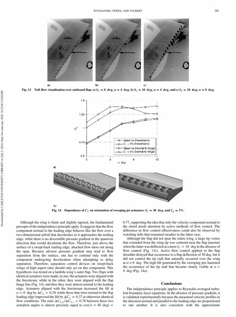
without actuation. Two hundred fifty exposures were taken over aperiod of 5 s and ensemble averaged onto a single picture. Thisaveraging allows differentiation between attached and separatedregions, one marked by stationary tufts and the other showing fansdue to oscillations around the anchor points (Fig. 13). Stationaryattached flow near the trailing edge was dominated by the spanwisecomponent because the streamwise component may possibly decel-erate below the freestream value (e.g., Fig. 6). In the absence of flapdeflection and at small angle of incidence α � 4 deg, weak spanwiseflow is observed (Fig. 13a). By increasing the lift, either throughincreased flap deflection or through angle of attack, the relativestrength of the spanwise flow has increased (Figs. 13b and 13c).Slightly unsteady flowmay be seen near the juncture between the flapand thewing tip. At α � 8 deg, the flow over thewing tip and at leasthalf of the outer flap is separated (Fig. 13c).
Fig. 11 Wall streamlines on a swept-back rectangular wing [12].
Fig. 12 Wing in test section.
180 WYGNANSKI, TEWES, AND TAUBERT
Dow
nloa
ded
by C
AR
LE
TO
N U
NIV
ER
SIT
Y L
IBR
AR
Y o
n Ju
ly 3
, 201
4 | h
ttp://
arc.
aiaa
.org
| D
OI:
10.
2514
/1.C
0322
06
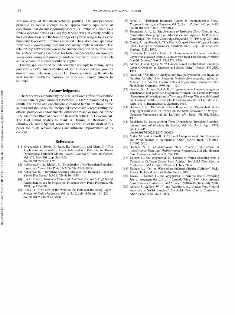
Although the wing is finite and slightly tapered, the fundamentalprecepts of the independence principle apply. It suggests that the flowcomponent normal to the leading edge behaves like the flow over atwo-dimensional airfoil that decelerates as it approaches the trailingedge, while there is no discernible pressure gradient in the spanwisedirection that would decelerate the flow. Therefore, just above thesurface of a swept-back trailing edge, attached flow turns out alongthe span. Because adverse pressure gradient may lead to flowseparation from the surface, one has to contend only with thecomponent undergoing deceleration when attempting to delayseparation. Therefore, separation control devices on swept-backwings of high aspect ratio should only act on this component. Thishypothesis was tested on a lambda wing’s outer flap. Two flaps withidentical actuators weremade; in one, the actuators were alignedwiththe freestream, while in the other, they were aligned with the flaphinge line (Fig. 14), and thus they were almost normal to the leadingedge. Actuators aligned with the freestream increased the lift atα � 0 deg byΔCL � 0.29, while those that were normal to the flapleading edge improved the lift byΔCL � 0.37 at otherwise identicalflow conditions. The ratio ΔCL;ξ∕ΔCL;x � 0.78 between these twoactuation angles is almost precisely equal to cos�Λ � 40 deg� �
0.77, supporting the idea that only the velocity component normal tothe chord needs attention by active methods of flow control. Thedifference in flow control effectiveness could also be observed bywatching tufts that remained steadier in the latter case.Although the flap did not span the entire wing, a large tip vortex
that extended from the wing tip was centered near the flap juncturewhen the latter was deflected at amere δf � 10 deg in the absence offlow control (Fig. 13c). Active flow control applied to the flapshoulder delayed that occurrence to a flap deflection of 30 deg, but itdid not control the tip stall that naturally occurred over the wingat α ≈ 6 deg. The high lift generated by the sweeping jets hastenedthe occurrence of the tip stall that became clearly visible at α �4 deg (Fig. 14a).
Conclusions
The independence principle applies to Reynolds-averaged turbu-lent boundary-layer equations. In the absence of pressure gradient, itis validated experimentally because the measured velocity profiles inthe direction normal and parallel to the leading edge are proportionalto one another. It is also consistent with the approximate
Fig. 13 Tuft flow visualization over outboard flap: a) δf � 0 deg, α � 4 deg, b) δf � 10 deg, α � 4 deg, and c) δf � 10 deg, α � 8 deg.
Fig. 14 Dependence of CL on orientation of sweeping jet actuators: δf � 30 deg, and Cμ � 3%.
WYGNANSKI, TEWES, AND TAUBERT 181
Dow
nloa
ded
by C
AR
LE
TO
N U
NIV
ER
SIT
Y L
IBR
AR
Y o
n Ju
ly 3
, 201
4 | h
ttp://
arc.
aiaa
.org
| D
OI:
10.
2514
/1.C
0322
06
self-similarity of the mean velocity profiles. The independenceprinciple is robust enough to be approximately applicable atconditions that do not rigorously accept its limitations, such as afinite-aspect-ratio wing or a slightly tapered wing. It clearly predictsthe flowdirection near the trailing edge of a yawedwing as long as theboundary layer over it remains attached. Thus, dominant spanwiseflow over a yawed wing does not necessarily imply separation. Therelationship between the yaw angle and the direction of the flow nearthe surface provides a rationale for turbulence modeling on complexswept-back wings and provides guidance for the direction in whichactive separation control should be applied.Finally, application of the independence principle to mixing layers
provides a better understanding of the turbulent mixing processdownstream of chevron nozzles [1]. However, extending the idea toheat transfer problems requires the turbulent Prandtl number tobe unity.
Acknowledgments
Thework was supported by the U.S. Air Force Office of ScientificResearch under grant number FA9550-10-01-0215 monitored by D.Smith. The views and conclusions contained herein are those of theauthors and should not be interpreted as necessarily representing theofficial policies or endorsements, either expressed or implied, of theU.S. Air ForceOffice of Scientific Research or the U.S. Government.The lead author wishes to thank A. Tumin, E. Reshotko, A.Shmilovich, and P. Spalart, whose frank criticism of the draft of thispaper led to its reexaminations and ultimate improvement of itscontent.
References
[1] Wygnanski, I., Tewes, P., Kurz, H., Taubert, L., and Chen, C., “TheApplication of Boundary Layer Independence Principle to Three-Dimensional Turbulent Mixing Layers,” Journal of Fluid Mechanics,Vol. 675, May 2011, pp. 336–346.doi:10.1017/jfm.2011.95
[2] Ashkenas, H., and Riddell, F., “Investigation of the Turbulent BoundaryLayer on a Yawed Flat Plate,” NACA TN-3383, 1955.
[3] Ashkenas, H., “Turbulent Shearing Stress in the Boundary Layer ofYawed Flat Plates,” NACA TN-4140, 1958.
[4] Lin, C. C. (ed.), Turbulent Flows and Heat Transfer, Vol. 5, High SpeedAerodynamics and Jet Propulsion, PrincetonUniv. Press, Princeton, NJ,1959, pp 156–158.
[5] Coles, D., “The Law of the Wake in the Turbulent Boundary Layer,”Journal of Fluid Mechanics, Vol. 1, No. 2, July 1956, pp. 191–226.doi:10.1017/S0022112056000135
[6] Rotta, J., “Turbulent Boundary Layers in Incompressible Flow,”Progress in Aerospace Sciences, Vol. 2, Nos. 1–2, Jan. 1962, pp. 1–95.doi:10.1016/0376-0421(62)90014-3
[7] Townsend, A. A. R., The Structure of Turbulent Shear Flow, 1st ed.,Cambridge Monographs on Mechanics and Applied Mathematics,CambridgeUniv. Press, Cambridge, England, U.K., 1956, pp. 224–261.
[8] Young, A., and Booth, T., “The Profile Drag of YawedWings of InfiniteSpan,” College of Aeronautics, Cranfield Univ., Rept. 38, Cranfield,England, U.K., 1950.
[9] Reshotko, E., and Beckwith, I., “Compressible Laminar BoundaryLayer over a Yawed Infinite Cylinder with Heat Transfer and ArbitraryPrandtl Number,” NACA TR-1379, 1958.
[10] Altman, J., and Hayter, N., “AComparison of the Turbulent Boundary-Layer Growth on an Unswept and Swept Wing,” NACA TN-2500,1951.
[11] Drela, M., “XFOIL: An Analysis and Design System for Low ReynoldsNumber Airfoils,” Low Reynolds Number Aerodynamics, edited byMueller, T. J., Vol. 54, Lecture Notes in Engineering, Springer–Berlin,Heidelberg, Germany, 1989, pp. 1–12.
[12] Gronau, K. H., and Nickel, K., “Experimentelle Untersuchungen anschiebenden und gepfeilten Flügeln mit Normal- und Laminar-Profilen(Experimental Investigations of Yawing and SweptWings with Normaland Laminar Profiles),” Deutsche Forschungsanstalt für Luftfahrt e.V.,Rept. 56/14, Braunschweig, Germany, 1956.
[13] Hoerner, S. F., “Einfluß der Pfeilstellung auf die Überziehbarkeit derTragflügel (Influence of Sweep on the Stall Behaviour of Wings),”Deutsche Versuchsanstalt für Luftfahrt e.V., Rept. PB-392, Berlin,1936.
[14] Bradshaw, P., “Calculation of Three-Dimensional Turbulent BoundaryLayers,” Journal of Fluid Mechanics, Vol. 46, No. 3, April 1971,pp. 417–445.doi:10.1017/S0022112071000624
[15] Malik, M., and Bushnell, D., “Role of Computational Fluid Dynamicsand Wind Tunnels in Aeronautics R&D,” NASA Rept. TP-2012-217602, 2010.
[16] Hoerner, S. F., Fluid-Dynamic Drag: Practical Information on
Aerodynamic Drag and Hydrodynamic Resistance, 2nd ed., HoernerFluid Dynamics, Bakersfield, CA, 1965.
[17] Taubert, L., and Wygnanski, I., “Control of Vortex Shedding from aCylinder at Different Sweep Back Angles,” 2nd AIAA Flow Control
Conference, AIAA Paper 2004-2511, June 2004.[18] Taubert, L., “On the Wake of an Inclined Circular Cylinder,” Ph.D.
Thesis, Technical Univ. of Berlin, Berlin, 2010.[19] Tewes, P., Taubert, L., and Wygnanski, I., “On the Use of Sweeping
Jets to Augment the Lift of a Lambda-Wing,” 28th AIAA Applied
Aerodynamics Conference, AIAA Paper 2010-4689, June–July 2010.[20] Anders, S., Sellers, W. III, and Washburn, A., “Active Flow Control
Activities at NASA Langley,” 2nd AIAA Flow Control Conference,AIAA Paper 2004-2623, 2004.
182 WYGNANSKI, TEWES, AND TAUBERT
Dow
nloa
ded
by C
AR
LE
TO
N U
NIV
ER
SIT
Y L
IBR
AR
Y o
n Ju
ly 3
, 201
4 | h
ttp://
arc.
aiaa
.org
| D
OI:
10.
2514
/1.C
0322
06