Applying wavelet-based hidden Markov tree to enhancing performance of process monitoring

Chemical Engineering Science 60 (2005) 5129–5143

www.elsevier.com/locate/ces

Applyingwavelet-based hiddenMarkov tree to enhancing performance ofprocessmonitoring

Junghui Chen∗, Wang-Jung ChangDepartment of Chemical Engineering, Chung-Yuan Christian University, Chung-Li, Taiwan 320, Republic of China

Accepted 1 March 2005Available online 6 June 2005

Abstract

In this paper, wavelet-based hidden Markov tree (HMT) models is proposed to enhance the conventional time-scale only statisticalprocess model (SPC) for process monitoring. HMT in the wavelet domain cannot only analyze the measurements at multiple scales intime and frequency but also capture the statistical behavior of real world measurements in these different scales. The former can providebetter noise reduction and less signal distortion than conventional filtering methods; the latter can extract the statistical characteristicsof the unmeasured disturbances, like the clustering and persistence of the practical data which are not considered in SPC. Based onHMT, a univariate and a multivariate SPC are respectively developed. Initially, the SPC model is trained in the wavelet domain usingthe data obtained from the normal operation regions. The model parameters are trained by the expectation maximization algorithm. Afterextracting the past operating information, the proposed method, like the philosophy of the traditional SPC, can generate simple monitoringcharts, easily tracking and monitoring the occurrence of observable upsets. The comparisons of the existing SPC methods that explain theadvantages of the properties of the newly proposed method are shown. They indicate that the proposed method can lead to more accurateresults. Data from the monitoring practice in the industrial problems are presented to help readers delve into the matter.� 2005 Elsevier Ltd. All rights reserved.

Keywords:Process monitoring; Principal component analysis; Statistical process control; Wavelet transform, Hidden Markov model

1. Introduction

Modern chemical plants are composed of various kindsof highly complex processes and many integrated units. Tosave energy and materials, the processes are often oper-ated at the extreme limit of pressure and temperature. Thismakes them susceptible to various failures that cause an un-acceptable deterioration of the performance or even lead todangerous situations. In order to produce uniformly high-quality products under the safe operation of the chemicalplant, monitoring operation processes is one of the most im-portant issues in the chemical industries. Statistical processcontrol (SPC) is a commonly used tool which can ensurethe quality of the manufactured product. Instead of using

∗ Corresponding author. Fax: +88633654199.E-mail address:[email protected](J. Chen).

0009-2509/$ - see front matter� 2005 Elsevier Ltd. All rights reserved.doi:10.1016/j.ces.2005.03.061

detailed mathematical models, it is mostly based on data-driven methods to extract the state of the system via applica-tions of statistical methods. The workhorse of SPC controlcharts, such as Shewhart chart, cumulative sum (CUSUM)and exponentially weighted moving average (EWMA), ap-plies well to monitoring process (Box and Luceno 1997;Montgomery, 1996). However, most industrial applicationsare multivariable in nature and the measured variables canbe highly correlated. The analysis will result in poor perfor-mance if the conventional SPC control charts are applied.Several advanced techniques have been developed for mul-tivariable statistical process control (MPSC). Hotelling’sT 2

statistics is one of the commonmethods of constructing mul-tivariable control charts (Mason et al., 1997; Sullivan andWoodall, 1996; Hotelling, 1947). The normalT 2 statisticscould change drastically for just a small change in the data ifthe data covariance matrix is nearly rank deficient. Principal

http://www.elsevier.com/locate/ces

mailto:[email protected]

5130 J. Chen, W.-J. Chang / Chemical Engineering Science 60 (2005) 5129–5143

component analysis (PCA) combined with statistics is prob-ably the most widely used multivariable technique in thechemical engineering field (Piovoso and Hoo, 2002; Krestaet al., 1991). It can extract a set of combinational variables,or major principal components, to describe the key varia-tions and trends for the operating data. The key measuredvariables from the PCA model give better understanding ofthe fault event taken place in the process. Even though thiscontrol method can decorrelate the measurements, this ap-proach is often not practical for industrial multivariate ap-plications with multiscale or autocorrelated measurements(Aradhye et al., 2003).Recently wavelet transformations appear as an efficient

tool for signal processing tasks, which can involve real-worlddata. They can localize the process information in the time-frequency plane with different resolutions. PCA has alsobeen applied to the information-rich signal representation ofthe wavelet transform in the chemical process for monitoringpurposes. Wavelet-based multi-scale PCA (MSPCA) basedon the assumption that the different process events makedifferent contributions at the time and frequency domainswas proposed (Bakshi, 1998). The multi-scale fault identifi-cation problem was applied in order to find out the differentprocess events at the corresponding frequency levels (Misraet al., 2002). A similarity measure based on the combina-tion of PCA and wavelet analysis was also developed foron-line process monitoring and fault diagnosis (Lu et al.,2003). However, the inter-scale dependencies of wavelet co-efficients existed (Crouse et al., 1998). The hidden Markovtree (HMT) structures adopted for the wavelet transformdescription could match these statistical characteristics ofnon-Gaussian data. It could improve the results of the signaldetection or resolutions. Using HMT, process trend classi-fication was recently proposed to analyze the correlationsamong variables across the time-frequency plane (Sun et al.,2003; Bakhtazad et al., 2000). While HTM revealed moreuseful features in the previous studies, the benefits of theHMT model are worthwhile to apply to the existing SPCmethods to enhance the capability of the statistical pro-cess monitoring. In this paper, MSPC control charts underwavelet-based HMT are developed. This approach cannotonly analyze themeasurements at multiple scales in time andfrequency, but also capture the clustering and persistence ofthe statistical characteristics for practical data.The remainder of this paper is organized as follows. Con-

ventional SPCs for univariate and multivariate are brieflyreviewed in the next section. Section 3 focuses on the struc-ture of the wavelet-based HMT and its application on sig-nal de-noising. The monitoring approach of the proposedmethod based on HMT is developed in Section 4. Its mon-itoring statistics are established to build up the confidencelimit. In Section 5, the performance of the proposed methodis investigated through two sets of benchmark data from theindustrial processes and a comparison with the conventionalPCA and MSPCA is made. Finally, a summary and someconclusions are presented.

2. Conventional SPC

In SPC monitoring techniques, the objective is to iden-tify assignable or special causes of variability and furtherto eliminate the causes to lead to stable processes. Theobservations (y(k)) in SPC approach basically from theShewhart–Deming statistical model can be represented bytwo parts:

y(k) = ys(k) + e(k)

= �0︸︷︷︸explained

+ e(k)︸︷︷︸unexplained

, (1)

wherey(k), the measurement of the process variable at timek, is represented by an explained system outputys(k) (whichis often estimated from the mean value of the data set rep-resentative of the period of normal performance,�0) plusan unexplained residuale(k), often called the random mea-surement error resulted from the uncertain variations anddisturbances among the lurking variables. When the processis operated in a state of control, the output deviation wouldbe independent and vary in a stable manner around the fixedmean�. The variatione(k), often called the common cause,is a white noise sequence,e(k) ∼ N(0,�2). Since manyoperating processes are driven by intertia element, the er-rorse(k) are not always independent, particularly when theinterval between samples become small relative to intertiaforces. As expected, the performance of the Shewhart modelwould be deteriorated as the process exhibits more and moreserial correlation. In the past research (Box and Luceno,1997; Astrom, 1970), it has been suggested that stochas-tic process control methods represent an appropriate exten-sion of traditional SPC methods into the domain of corre-lated processes. However, the prior model structure is notknown. The trial-and-error procedure is often needed to de-termine the proper model structure from the measured dataset. Although the model can effectively detect the abnormalsituation for the correlated disturbance, the false detectionsare often inevitable because of the disturbance of variabilityfrom the different scale levels.As for the multivariable system, it can also be represented

by two parts, an explained system output vector (ys(k)) andan unexplained residual vector (e),

y(k) = ys(k) + e= �0 + � + e= �0 + Pt︸︷︷︸

explained

+ e︸︷︷︸unexplained

, (2)

where�0 is the vector of the desired mean values. In the fol-lowing measured variables (y), assume that they have beenmean centered (i.e.,�0 = 0) without further more explana-tion. � is the correlated vector among the measured vari-ables. It can be decomposed in terms ofr linear principalcomponents (P ∈ Rn×r ) with r �n, and t ∈ Rr is definedas the principal component scores which are the projec-tions of y ontoP. When the process is operated in a state

J. Chen, W.-J. Chang / Chemical Engineering Science 60 (2005) 5129–5143 5131

of control, the expected distribution ofe(k) should be nor-mally distributed withe(k) ∼ N(0,�) where� is covari-ance matrix. Based on the concept of the Shewart controlchart, fault detection can analyze the statistical characteris-tics ofe(k) to qualify the actual state of the process: normalor faulty. Like the discussion on the univariate, the moni-toring based on the conventional MSPC for the multivari-ate may also lead to wrong detection as the process con-tains the measurement noise and exhibits more and moreserial correlation. Past research shows the wavelet transformcan filter and decompose the measurements under the multi-resolution wavelet transform. Although the noise levels aresuccessfully removed to indicate the status of the processsystem behavior (Nason, 1996), the distribution of the de-composed signal in the wavelet domain is not considered. Inthis research, a wavelet-based HMT model, which can de-scribe the distribution of the wavelet coefficients, is appliedto extract the unexplainable (or stochastic) part of the pro-cess information and to further improve the performance ofthe conventional SPC and MSPCmodels. Before developingthe proposed SPC model, the relevant notations and the ad-vantageous properties of HMT are briefly introduced first.

3. Hidden Markov tree model

HMT (Crouse et al., 1998) is the extension version ofthe time domain of the chain structure of hidden Markovmodel (HMM) (Rabiner, 1989) into a wavelet domain of thetree structure for signal classification. Unlike HMM onlyconsidering measurements at one resolution, HMT has thedesired signal distributions which locate and cluster at sometime-frequency frames. HMT is a tree consisting of a set ofthe hierarchy nodes (Fig. 1). Each wavelet coefficient (ornode) has a hidden backbone that contains a finite numberof states, where the state in a node is only dependent on itsimmediate parent and any children it may have. It is modeledby an underlying stochastic process that is not observable(i.e., it is hidden). It is a state transitional process describedby the state transition probabilities that give the transitionprobabilities from one state to itself or any other states in asingle step.Assuming that the wavelet coefficients are divided intoM

states, each wavelet coefficient (wi) is associated to a dis-crete hidden stateSi =m,m ∈ {1,2, . . . , M}. The Gaussiandensity (�(wi |Si = m)) is defined as the stateSi with themean�i,m and the variance�2i,m. The overall density of thewavelet coefficient (wi) is given by

f (wi) =M∑

m=1psi(m)�(wi |Si = m), (3)

where

�(wi |Si = m) = 1√2��2i,m

exp

[− (wi − �i,m)2

2�2i,m

](4)

1

2 3

5 64 7

nodeS1 S2

SN

t

f

1S

S1 S1 S1

S12S

S2 S2 S2 S2S1

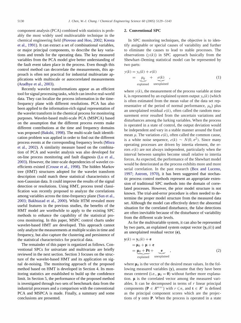
Fig. 1. The HMT structure of the multi-scale wavelet coefficients for adecomposed measurement in the wavelet domain. The wavelet coefficientsand their hidden state variables are denoted by gray and white nodes,respectively.

0 50 100 150 200 250-2

-1

0

1

2

3

4

5

Samples

y

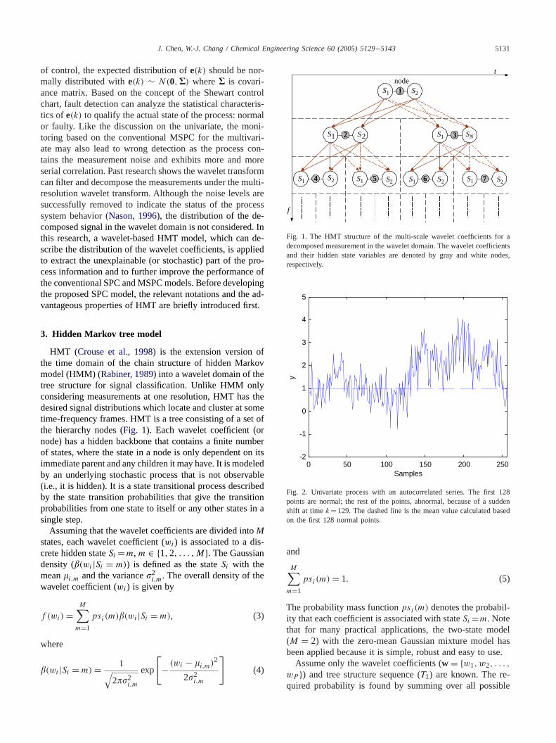
Fig. 2. Univariate process with an autocorrelated series. The first 128points are normal; the rest of the points, abnormal, because of a suddenshift at timek =129. The dashed line is the mean value calculated basedon the first 128 normal points.

and

M∑m=1

psi(m) = 1. (5)

The probability mass functionpsi(m) denotes the probabil-ity that each coefficient is associated with stateSi =m. Notethat for many practical applications, the two-state model(M = 2) with the zero-mean Gaussian mixture model hasbeen applied because it is simple, robust and easy to use.Assume only the wavelet coefficients (w = {w1, w2, . . . ,

wP }) and tree structure sequence (T1) are known. The re-quired probability is found by summing over all possible


65 + 192-1

0

1

D1

65 + 192-1

0

1

65 + 192

65 + 192 65 + 192 65 + 192

-1

0

1

-1

0

1

D2

-1

0

1

-1

0

1

64 96 + 160 192-1

0

1

D3

65 + 192-1

0

1

65 + 192-1

0

1

65 + 192-1

0

1

D4

65 + 192-1

0

1

65 + 192-1

0

1

64 + 192-1

0

1

D5

65 + 192-1

0

1

65 + 192-1

0

1

-1

0

1

D6 0

1

-1

0

1

65 + 192-1

0

1

D7

65 + 192-1

0

1

65 + 192

65 + 192 65 + 192 65 + 192

-1

0

1

65 || 1921

1.5

2

A7

65 || 1921

1.5

2

65 || 1921

1.5

2

65 128 192

0

2

4

y

65 128 192

0

2

4

65 128 192

0

2

4

SamplesSamplesSamples (b)(a) (c)

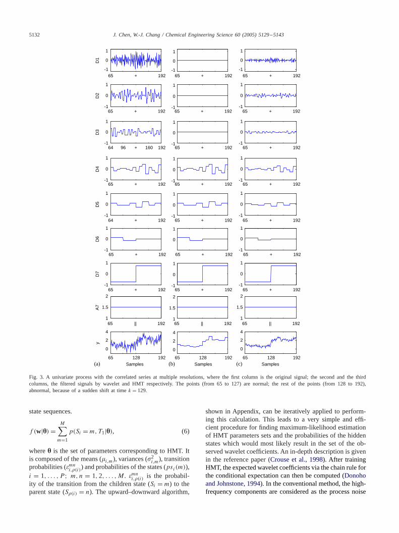
Fig. 3. A univariate process with the correlated series at multiple resolutions, where the first column is the original signal; the second and the thirdcolumns, the filtered signals by wavelet and HMT respectively. The points (from 65 to 127) are normal; the rest of the points (from 128 to 192),abnormal, because of a sudden shift at timek = 129.

state sequences.

f (w|�) =M∑

m=1p(Si = m, T1|�), (6)

where� is the set of parameters corresponding to HMT. Itis composed of the means (�i,m), variances (�

2i,m), transition

probabilities (�mni,�(i)) and probabilities of the states (psi(m)),

i = 1, . . . , P ; m, n = 1,2, . . . , M. �mni,�(i) is the probabil-

ity of the transition from the children state (Si = m) to theparent state (S�(i) = n). The upward–downward algorithm,

shown in Appendix, can be iteratively applied to perform-ing this calculation. This leads to a very simple and effi-cient procedure for finding maximum-likelihood estimationof HMT parameters sets and the probabilities of the hiddenstates which would most likely result in the set of the ob-served wavelet coefficients. An in-depth description is givenin the reference paper (Crouse et al., 1998). After trainingHMT, the expected wavelet coefficients via the chain rule forthe conditional expectation can then be computed (Donohoand Johnstone, 1994). In the conventional method, the high-frequency components are considered as the process noise


and they are removed; however, the HMTmodel includes thepossible contribution of the process behavior from the highfrequency components. Here a process measurement with ahighly serial correlation shown inFig. 2 is explained. A sus-tained shift is induced at time 129. It seems to be difficult todistinguish the normal from the abnormal shift event in thetime domain due to the autocorrelation of the measurements.The original signal is filtered through the wavelet and HMTde-noising procedure at multiple resolutions (Fig. 3). At thebottom of each column ofFig. 3, the extractions of the mea-sured signals are the reconstructed originals and the filteredoutputs by summing each column. In the multi-resolutionplots, it is obvious that the HMT model keep some infor-mation at the higher scaled resolution and it can properlyextract the change of the process behavior.

4. HMT based process monitoring scheme

The process monitoring structure under wavelet-basedHMT consists essentially of two core stages: the HMT-basedSPCmodel and HTM-based control charts. The control chartis related to the actual behavior of the process to be su-pervised compared with that of nominal model-observationfeatures driven by the nominal inputs. This allows findinga difference with respect to the normal operating conditionat the predefined threshold from the normal operating sta-tistical analysis. It also helps determine if the new processbehavior is referenced against this normal or in-control sta-tistical behavior.

4.1. HMT-based univariate SPC

Reconsider a single measurement with additive noisemodel:

y(k) = �0 + e(k). (7)

As mentioned in Section 2, the disturbancee(k) is not com-pletely uncorrelated. The objective of this control charts isto extract the possible process behavior within the signale(k) based on the observationy(k).First the residual parte(k) is simply obtained by deducting

themean value from the observations. The extractionmethodin the wavelet domain is based on taking the discrete wavelettransform (DWT) of the signale(k), passing this transformthrough the HMT modeling procedures, which removes thecoefficient below a certain value, then taking the inverseDWT. Finally, the measurement can be represented as

y(k) = �0 + sHMT(k)︸︷︷︸explained

+ �(k)︸︷︷︸unexplained

= yHMTs (k) + �(k), (8)

where sHMT(k) represents the stochastic disturbances ex-tracted frome(k) (Eq. (7)), and�(k) is unexplainable partfrom the residual.

The monitoring statistics of HMT are implemented in amanner similar to those of the conventional. Based on thehistorical data collected under the normal operating condi-tion, the SPC statistics at samplek is defined as

SPE(k) = (y(k) − (�0 + sHMT(k)))2, (9)

where SPE(k) is defined as the squares of�(k). Unlike thetraditional Shewart’s control chart with only one statisticsfor the disturbance (�(k)), the statistics (I2s ) based on theidentity of the lurking variablesHMT(k) from the disturbanceis defined as

I2s (k) = yHMTs (k)2. (10)

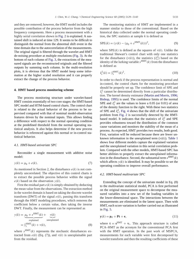
In order to check if the process representation is normal andin-control, the control charts for the monitoring procedureshould be properly set up. The confidence limit of SPE andI2s cannot be determined directly from a particular distribu-tion. The kernel density estimator (Martin and Morris, 1996;Bishop, 1995) is used. The confidence limits of the normalSPE andI2s are the values to leave a 0.05 (or 0.01) of areaof the density function to the right. With these two statisticsof SPE andI2s , Fig. 4 shows that the shift of the univariateproblem fromFig. 2 is successfully detected by the HMT-based model. It indicates that the statistics ofI2s and SPEprovides robustness toward the distribution of the commoncause variations and monitors the stability of the mean of aprocess. As expected, HMT provides two results, both good.First, variation will be reduced because there are fewer un-known information in the unexplained term (�(k)). Table 1shows four different models capture the explained variationand the unexplained variation in this serial correlation prob-lem. Compared with the other models, HMT-based SPC hasbetter abilities to properly extract the unexplained informa-tion in the disturbance. Second, the substantial termsHMT(k)

which affectsy(k) is identified. It may be possible to set theoperating condition to improve overall performance.

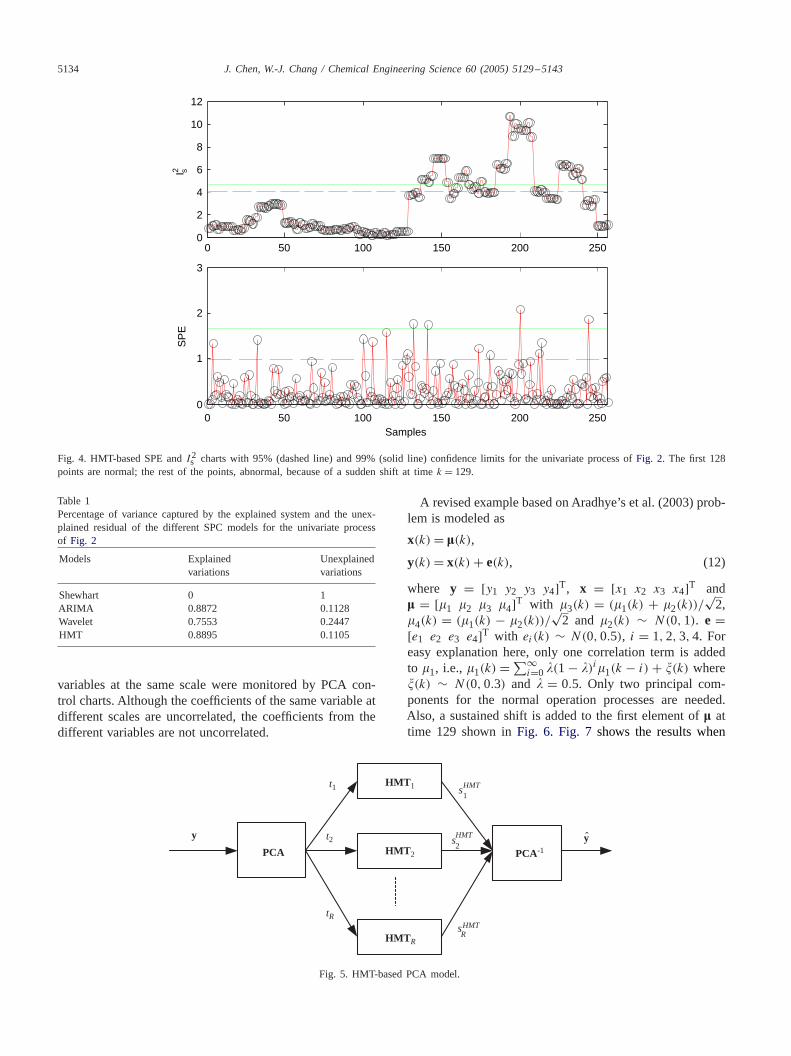
4.2. HMT-based multivariate SPC

Extending the concept of the univariate model in Eq. (8)to the multivariate statistical model, PCA is first performedon the original measurement space to decompose the mea-sured variables into a new set of the loading variables inthe lower-dimensional space. The interactions between themeasurements are eliminated in the latent space. Then withHMT, each score variation is further carried out as illustratedin Fig. 5.

y(k) = �0 + Pt + e, (11)

where t = sHMT + �t . This approach structure is calledPCA–HMT as the acronym for the conventional PCA firstwith the HMT operation. In the past work of MSPCA,measurements for each variable were first decomposed bywavelet transform and then the resulting coefficients of these


0 50 100 150 200 2500

1

2

3

Samples

SP

E

0 50 100 150 200 2500

2

4

6

8

10

12

I s2

Fig. 4. HMT-based SPE andI2s charts with 95% (dashed line) and 99% (solid line) confidence limits for the univariate process ofFig. 2. The first 128points are normal; the rest of the points, abnormal, because of a sudden shift at timek = 129.

Table 1Percentage of variance captured by the explained system and the unex-plained residual of the different SPC models for the univariate processof Fig. 2

Models Explained Unexplainedvariations variations

Shewhart 0 1ARIMA 0.8872 0.1128Wavelet 0.7553 0.2447HMT 0.8895 0.1105

variables at the same scale were monitored by PCA con-trol charts. Although the coefficients of the same variable atdifferent scales are uncorrelated, the coefficients from thedifferent variables are not uncorrelated.

y

t1 HMTs1

y

HMT 2

HMT 1

HMT R

t2

tR

PCA PCA-1

HMTs2

HMTRs

Fig. 5. HMT-based PCA model.

A revised example based on Aradhye’s et al. (2003) prob-lem is modeled as

x(k) = �(k),

y(k) = x(k) + e(k), (12)

where y = [y1 y2 y3 y4]T, x = [x1 x2 x3 x4]T and� = [�1 �2 �3 �4]T with �3(k) = (�1(k) + �2(k))/

√2,

�4(k) = (�1(k) − �2(k))/√2 and �2(k) ∼ N(0,1). e =

[e1 e2 e3 e4]T with ei(k) ∼ N(0,0.5), i = 1,2,3,4. Foreasy explanation here, only one correlation term is addedto �1, i.e.,�1(k) = ∑∞

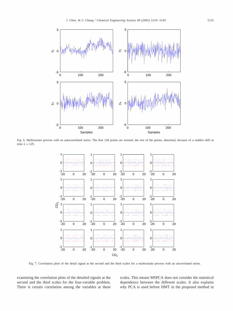
i=0 �(1− �)i�1(k − i) + (k) where(k) ∼ N(0,0.3) and � = 0.5. Only two principal com-ponents for the normal operation processes are needed.Also, a sustained shift is added to the first element of� attime 129 shown inFig. 6. Fig. 7 shows the results when


0 100 200-5

0

5

y 1 y 2y 4

0 100 200-5

0

5

0 100 200-5

0

5

Samples

y 3

0 100 200-5

0

5

Samples

Fig. 6. Multivariate process with an autocorrelated series. The first 128 points are normal; the rest of the points, abnormal, because of a sudden shiftattime k = 129.

-20 0 20-1

0

1

-20 0 20-1

0

1

-20 0 20-1

0

1

-20 0 20-1

0

1

-20 0 20-1

0

1

-20 0 20-1

0

1

-20 0 20-1

0

1

-20 0 20-1

0

1

-20 0 20-1

0

1

-20 0 20-1

0

1

-20 0 20-1

0

1

-20 0 20-1

0

1

-20 0 20-1

0

1

-20 0 20-1

0

1

-20 0 20-1

0

1

-20 0 20-1

0

1

CD

3

CD2

Fig. 7. Correlation plots of the detail signal at the second and the third scales for a multivariate process with an uncorrelated series.

examining the correlation plots of the detailed signals at thesecond and the third scales for the four-variable problem.There is certain correlation among the variables at these

scales. This means MSPCA does not consider the statisticaldependence between the different scales. It also explainswhy PCA is used before HMT in the proposed method in


0 50 100 150 200 2500

5

10

15

Samples

SP

E1

0 50 100 150 200 2500

0.5

1

1.5

2

I2 s1

0 50 100 150 200 2500

1

2

3

4

5

Samples

SP

E2

0 50 100 150 200 2500

5

10

15

I2 s2

(a)

(b)

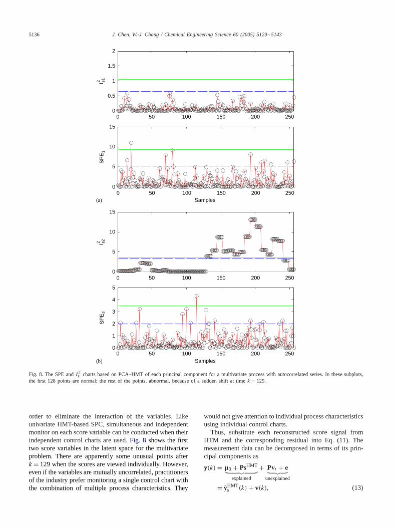
Fig. 8. The SPE andI2s charts based on PCA–HMT of each principal component for a multivariate process with autocorrelated series. In these subplots,the first 128 points are normal; the rest of the points, abnormal, because of a sudden shift at timek = 129.

order to eliminate the interaction of the variables. Likeunivariate HMT-based SPC, simultaneous and independentmonitor on each score variable can be conducted when theirindependent control charts are used.Fig. 8 shows the firsttwo score variables in the latent space for the multivariateproblem. There are apparently some unusual points afterk = 129 when the scores are viewed individually. However,even if the variables are mutually uncorrelated, practitionersof the industry prefer monitoring a single control chart withthe combination of multiple process characteristics. They

would not give attention to individual process characteristicsusing individual control charts.Thus, substitute each reconstructed score signal from

HTM and the corresponding residual into Eq. (11). Themeasurement data can be decomposed in terms of its prin-cipal components as

y(k) = �0 + PsHMT︸︷︷︸explained

+ P�t + e︸︷︷︸unexplained

= yHMTs (k) + v(k), (13)


0 50 100 150 200 2500

2

4

6

8

10

12

I s2

0 50 100 150 200 2500

5

10

15

SP

E

Samples

Fig. 9. PCA–HMT based SPE andI2s charts for the multivariate processwith the correlated series. The first 128 points are normal; the rest of thepoints, abnormal, because of a sudden shift at timek = 129.

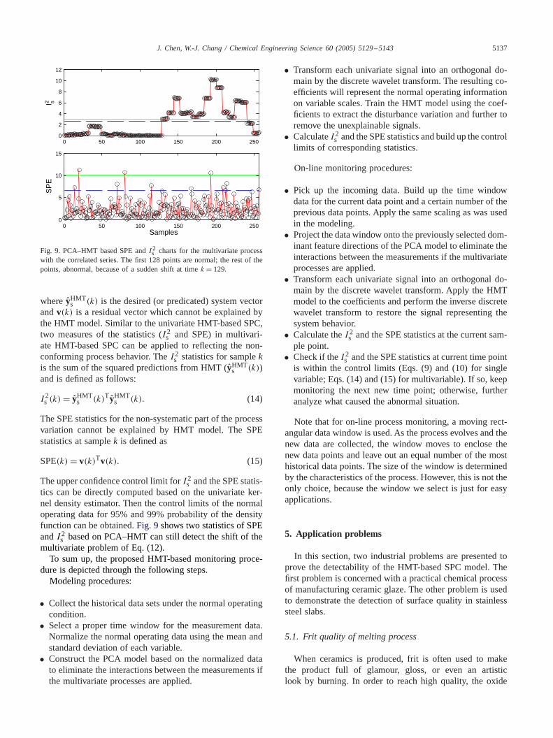
whereyHMTs (k) is the desired (or predicated) system vectorandv(k) is a residual vector which cannot be explained bythe HMT model. Similar to the univariate HMT-based SPC,two measures of the statistics (I2s and SPE) in multivari-ate HMT-based SPC can be applied to reflecting the non-conforming process behavior. TheI2s statistics for samplekis the sum of the squared predictions from HMT (yHMTs (k))and is defined as follows:

I2s (k) = yHMTs (k)TyHMTs (k). (14)

The SPE statistics for the non-systematic part of the processvariation cannot be explained by HMT model. The SPEstatistics at samplek is defined as

SPE(k) = v(k)Tv(k). (15)

The upper confidence control limit forI2s and the SPE statis-tics can be directly computed based on the univariate ker-nel density estimator. Then the control limits of the normaloperating data for 95% and 99% probability of the densityfunction can be obtained.Fig. 9shows two statistics of SPEandI2s based on PCA–HMT can still detect the shift of themultivariate problem of Eq. (12).To sum up, the proposed HMT-based monitoring proce-

dure is depicted through the following steps.Modeling procedures:

• Collect the historical data sets under the normal operatingcondition.

• Select a proper time window for the measurement data.Normalize the normal operating data using the mean andstandard deviation of each variable.

• Construct the PCA model based on the normalized datato eliminate the interactions between the measurements ifthe multivariate processes are applied.

• Transform each univariate signal into an orthogonal do-main by the discrete wavelet transform. The resulting co-efficients will represent the normal operating informationon variable scales. Train the HMT model using the coef-ficients to extract the disturbance variation and further toremove the unexplainable signals.

• CalculateI2s and the SPE statistics and build up the controllimits of corresponding statistics.

On-line monitoring procedures:

• Pick up the incoming data. Build up the time windowdata for the current data point and a certain number of theprevious data points. Apply the same scaling as was usedin the modeling.

• Project the data window onto the previously selected dom-inant feature directions of the PCA model to eliminate theinteractions between the measurements if the multivariateprocesses are applied.

• Transform each univariate signal into an orthogonal do-main by the discrete wavelet transform. Apply the HMTmodel to the coefficients and perform the inverse discretewavelet transform to restore the signal representing thesystem behavior.

• Calculate theI2s and the SPE statistics at the current sam-ple point.

• Check if theI2s and the SPE statistics at current time pointis within the control limits (Eqs. (9) and (10) for singlevariable; Eqs. (14) and (15) for multivariable). If so, keepmonitoring the next new time point; otherwise, furtheranalyze what caused the abnormal situation.

Note that for on-line process monitoring, a moving rect-angular data window is used. As the process evolves and thenew data are collected, the window moves to enclose thenew data points and leave out an equal number of the mosthistorical data points. The size of the window is determinedby the characteristics of the process. However, this is not theonly choice, because the window we select is just for easyapplications.

5. Application problems

In this section, two industrial problems are presented toprove the detectability of the HMT-based SPC model. Thefirst problem is concerned with a practical chemical processof manufacturing ceramic glaze. The other problem is usedto demonstrate the detection of surface quality in stainlesssteel slabs.

5.1. Frit quality of melting process

When ceramics is produced, frit is often used to makethe product full of glamour, gloss, or even an artisticlook by burning. In order to reach high quality, the oxide


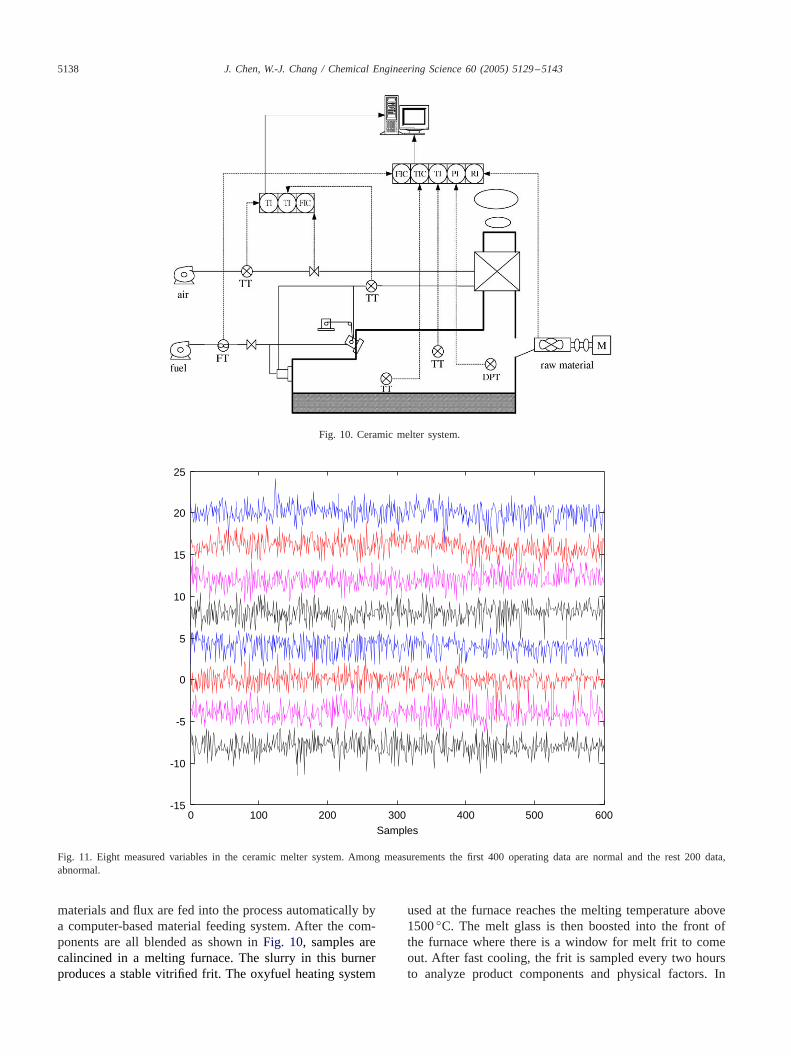
Fig. 10. Ceramic melter system.

0 100 200 300 400 500 600-15

-10

-5

0

5

10

15

20

25

Samples

Fig. 11. Eight measured variables in the ceramic melter system. Among measurements the first 400 operating data are normal and the rest 200 data,abnormal.

materials and flux are fed into the process automatically bya computer-based material feeding system. After the com-ponents are all blended as shown inFig. 10, samples arecalincined in a melting furnace. The slurry in this burnerproduces a stable vitrified frit. The oxyfuel heating system

used at the furnace reaches the melting temperature above1500◦C. The melt glass is then boosted into the front ofthe furnace where there is a window for melt frit to comeout. After fast cooling, the frit is sampled every two hoursto analyze product components and physical factors. In


0 50 100 150 200 250 3000

5

10

15

Samples

SP

E

0 50 100 150 200 250 3000

10

20

30

T2

0 50 100 150 200 250 3000

50

100

150

T2

0 50 100 150 200 250 3000

5

10

15

SP

E

Samples(a) (b)

0 50 100 150 200 250 3000

10

20

30

40

Samples

SP

E

0 50 100 150 200 250 3000

1

2

3

4

I2 s

(c)

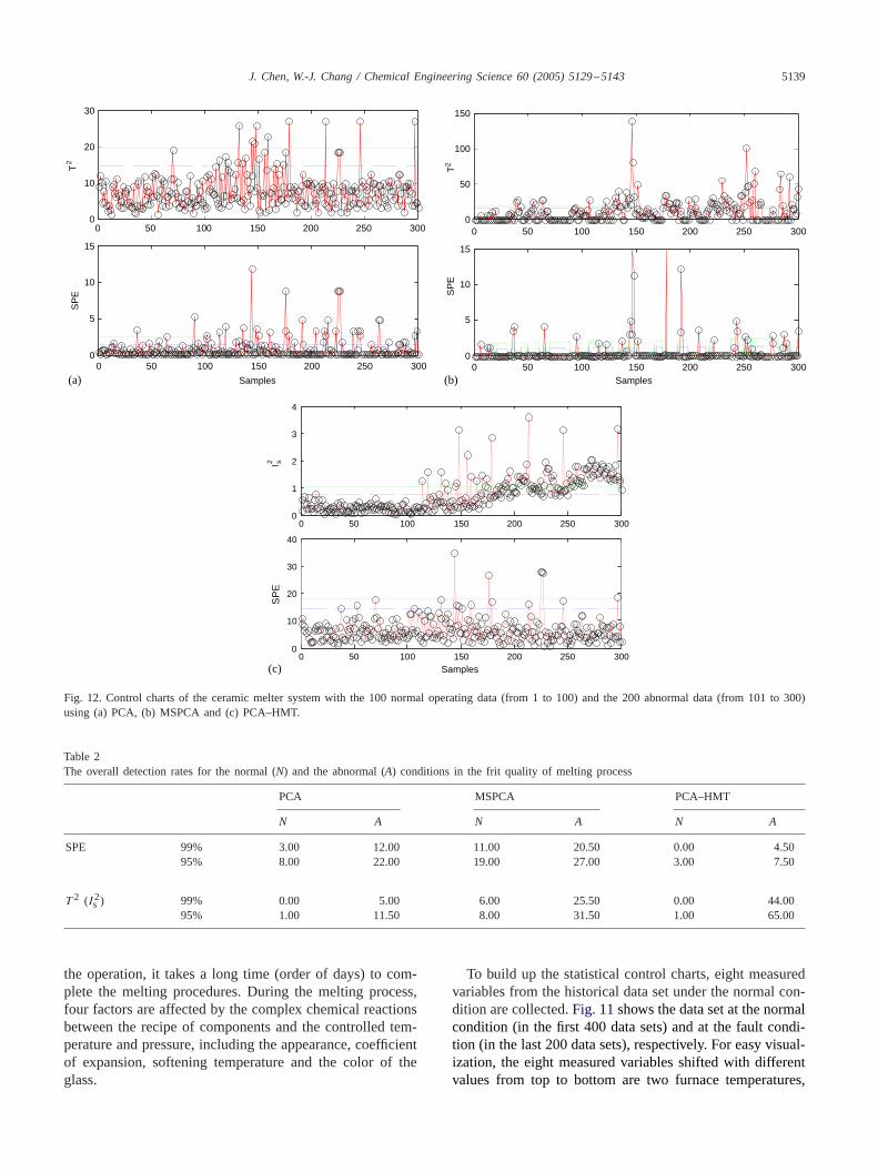
Fig. 12. Control charts of the ceramic melter system with the 100 normal operating data (from 1 to 100) and the 200 abnormal data (from 101 to 300)using (a) PCA, (b) MSPCA and (c) PCA–HMT.

Table 2The overall detection rates for the normal (N) and the abnormal (A) conditions in the frit quality of melting process

PCA MSPCA PCA–HMT

N A N A N A

SPE 99% 3.00 12.00 11.00 20.50 0.00 4.5095% 8.00 22.00 19.00 27.00 3.00 7.50

T 2 (I2s ) 99% 0.00 5.00 6.00 25.50 0.00 44.0095% 1.00 11.50 8.00 31.50 1.00 65.00

the operation, it takes a long time (order of days) to com-plete the melting procedures. During the melting process,four factors are affected by the complex chemical reactionsbetween the recipe of components and the controlled tem-perature and pressure, including the appearance, coefficientof expansion, softening temperature and the color of theglass.

To build up the statistical control charts, eight measuredvariables from the historical data set under the normal con-dition are collected.Fig. 11shows the data set at the normalcondition (in the first 400 data sets) and at the fault condi-tion (in the last 200 data sets), respectively. For easy visual-ization, the eight measured variables shifted with differentvalues from top to bottom are two furnace temperatures,


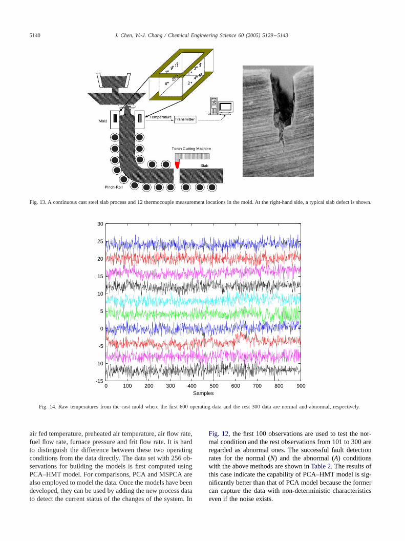
Fig. 13. A continuous cast steel slab process and 12 thermocouple measurement locations in the mold. At the right-hand side, a typical slab defect is shown.

0 100 200 300 400 500 600 700 800 900-15

-10

-5

0

5

10

15

20

25

30

Samples

Fig. 14. Raw temperatures from the cast mold where the first 600 operating data and the rest 300 data are normal and abnormal, respectively.

air fed temperature, preheated air temperature, air flow rate,fuel flow rate, furnace pressure and frit flow rate. It is hardto distinguish the difference between these two operatingconditions from the data directly. The data set with 256 ob-servations for building the models is first computed usingPCA–HMT model. For comparisons, PCA and MSPCA arealso employed to model the data. Once the models have beendeveloped, they can be used by adding the new process datato detect the current status of the changes of the system. In

Fig. 12, the first 100 observations are used to test the nor-mal condition and the rest observations from 101 to 300 areregarded as abnormal ones. The successful fault detectionrates for the normal (N) and the abnormal (A) conditionswith the above methods are shown inTable 2. The results ofthis case indicate the capability of PCA–HMT model is sig-nificantly better than that of PCA model because the formercan capture the data with non-deterministic characteristicseven if the noise exists.


0

5

10

15

Samples

SP

E

0 100 200 300 400 500 600 0 100 200 300 400 500 600

0 100 200 300 400 500 600 0 100 200 300 400 500 600

0 100 200 300 400 500 600

0

10

20

30

40

50

T2

0

0.5

1

1.5

2x 1012

T2

0

10

20

30

SPE

Samples

0 100 200 300 400 500 600

Samples

0

10

20

30

40

SP

E

0

2

4

6

8

I2 s

(a) (b)

(c)

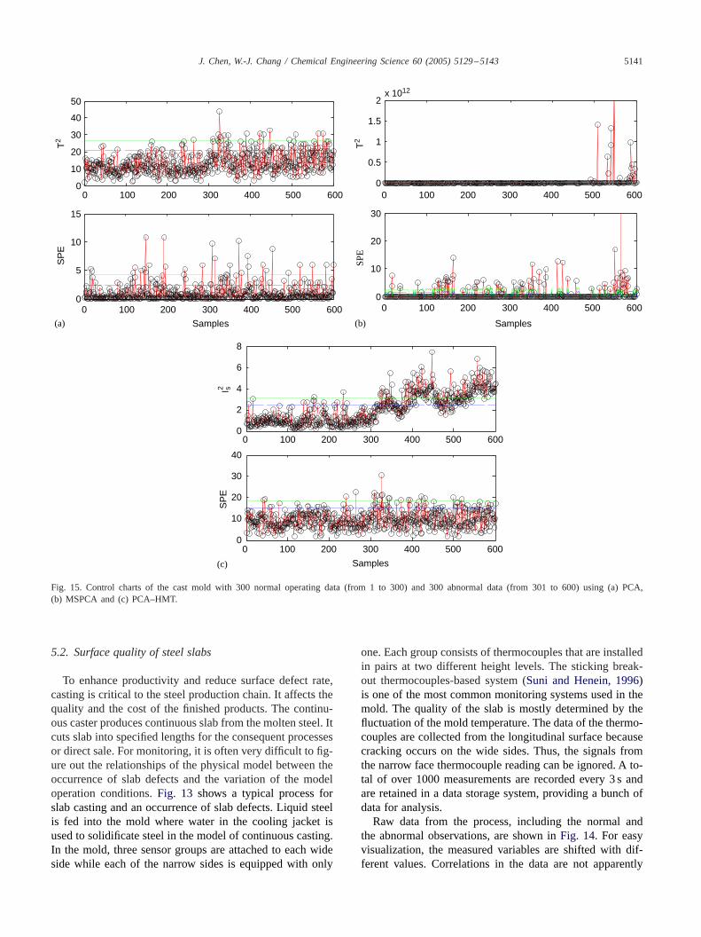
Fig. 15. Control charts of the cast mold with 300 normal operating data (from 1 to 300) and 300 abnormal data (from 301 to 600) using (a) PCA,(b) MSPCA and (c) PCA–HMT.

5.2. Surface quality of steel slabs

To enhance productivity and reduce surface defect rate,casting is critical to the steel production chain. It affects thequality and the cost of the finished products. The continu-ous caster produces continuous slab from the molten steel. Itcuts slab into specified lengths for the consequent processesor direct sale. For monitoring, it is often very difficult to fig-ure out the relationships of the physical model between theoccurrence of slab defects and the variation of the modeloperation conditions.Fig. 13 shows a typical process forslab casting and an occurrence of slab defects. Liquid steelis fed into the mold where water in the cooling jacket isused to solidificate steel in the model of continuous casting.In the mold, three sensor groups are attached to each wideside while each of the narrow sides is equipped with only

one. Each group consists of thermocouples that are installedin pairs at two different height levels. The sticking break-out thermocouples-based system (Suni and Henein, 1996)is one of the most common monitoring systems used in themold. The quality of the slab is mostly determined by thefluctuation of the mold temperature. The data of the thermo-couples are collected from the longitudinal surface becausecracking occurs on the wide sides. Thus, the signals fromthe narrow face thermocouple reading can be ignored. A to-tal of over 1000 measurements are recorded every 3 s andare retained in a data storage system, providing a bunch ofdata for analysis.Raw data from the process, including the normal and

the abnormal observations, are shown inFig. 14. For easyvisualization, the measured variables are shifted with dif-ferent values. Correlations in the data are not apparently


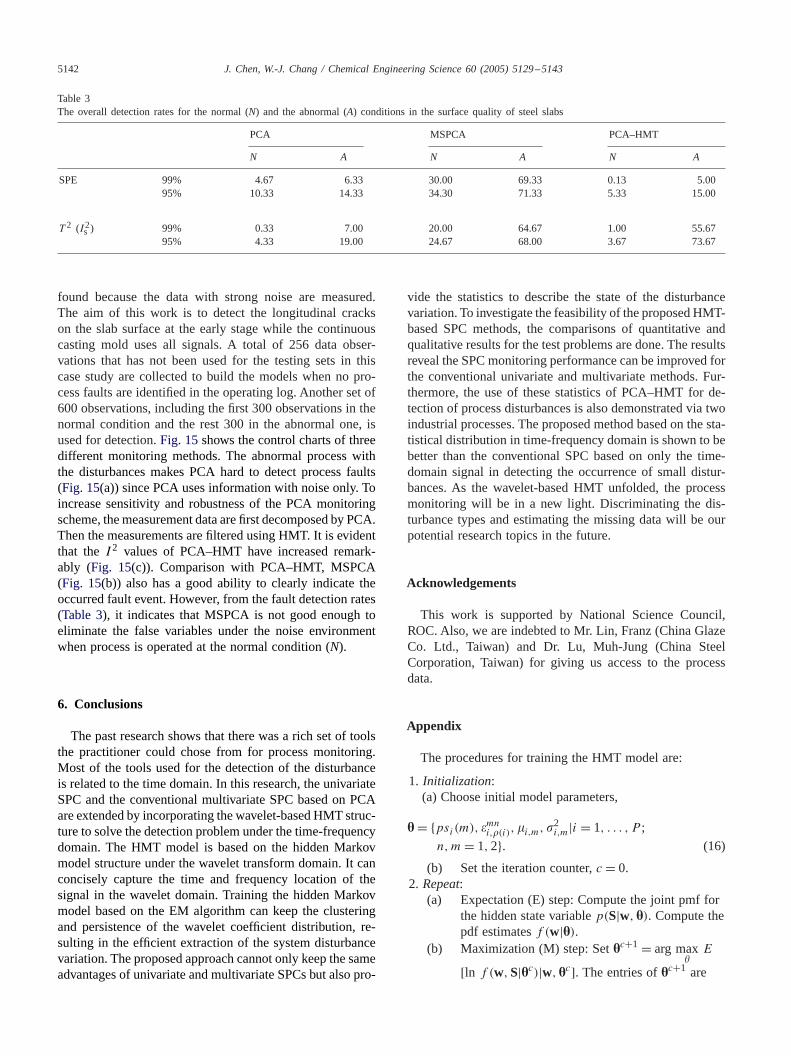
Table 3The overall detection rates for the normal (N) and the abnormal (A) conditions in the surface quality of steel slabs

PCA MSPCA PCA–HMT

N A N A N A

SPE 99% 4.67 6.33 30.00 69.33 0.13 5.0095% 10.33 14.33 34.30 71.33 5.33 15.00

T 2 (I2s ) 99% 0.33 7.00 20.00 64.67 1.00 55.6795% 4.33 19.00 24.67 68.00 3.67 73.67

found because the data with strong noise are measured.The aim of this work is to detect the longitudinal crackson the slab surface at the early stage while the continuouscasting mold uses all signals. A total of 256 data obser-vations that has not been used for the testing sets in thiscase study are collected to build the models when no pro-cess faults are identified in the operating log. Another set of600 observations, including the first 300 observations in thenormal condition and the rest 300 in the abnormal one, isused for detection.Fig. 15shows the control charts of threedifferent monitoring methods. The abnormal process withthe disturbances makes PCA hard to detect process faults(Fig. 15(a)) since PCA uses information with noise only. Toincrease sensitivity and robustness of the PCA monitoringscheme, themeasurement data are first decomposed by PCA.Then the measurements are filtered using HMT. It is evidentthat theI2 values of PCA–HMT have increased remark-ably (Fig. 15(c)). Comparison with PCA–HMT, MSPCA(Fig. 15(b)) also has a good ability to clearly indicate theoccurred fault event. However, from the fault detection rates(Table 3), it indicates that MSPCA is not good enough toeliminate the false variables under the noise environmentwhen process is operated at the normal condition (N).

6. Conclusions

The past research shows that there was a rich set of toolsthe practitioner could chose from for process monitoring.Most of the tools used for the detection of the disturbanceis related to the time domain. In this research, the univariateSPC and the conventional multivariate SPC based on PCAare extended by incorporating the wavelet-based HMT struc-ture to solve the detection problem under the time-frequencydomain. The HMT model is based on the hidden Markovmodel structure under the wavelet transform domain. It canconcisely capture the time and frequency location of thesignal in the wavelet domain. Training the hidden Markovmodel based on the EM algorithm can keep the clusteringand persistence of the wavelet coefficient distribution, re-sulting in the efficient extraction of the system disturbancevariation. The proposed approach cannot only keep the sameadvantages of univariate and multivariate SPCs but also pro-

vide the statistics to describe the state of the disturbancevariation. To investigate the feasibility of the proposed HMT-based SPC methods, the comparisons of quantitative andqualitative results for the test problems are done. The resultsreveal the SPCmonitoring performance can be improved forthe conventional univariate and multivariate methods. Fur-thermore, the use of these statistics of PCA–HMT for de-tection of process disturbances is also demonstrated via twoindustrial processes. The proposed method based on the sta-tistical distribution in time-frequency domain is shown to bebetter than the conventional SPC based on only the time-domain signal in detecting the occurrence of small distur-bances. As the wavelet-based HMT unfolded, the processmonitoring will be in a new light. Discriminating the dis-turbance types and estimating the missing data will be ourpotential research topics in the future.

Acknowledgements

This work is supported by National Science Council,ROC. Also, we are indebted to Mr. Lin, Franz (China GlazeCo. Ltd., Taiwan) and Dr. Lu, Muh-Jung (China SteelCorporation, Taiwan) for giving us access to the processdata.

Appendix

The procedures for training the HMT model are:

1. Initialization:(a) Choose initial model parameters,

� = {psi(m), �mni,�(i),�i,m,�2i,m|i = 1, . . . , P ;

n, m = 1,2}. (16)

(b) Set the iteration counter,c = 0.2.Repeat:

(a) Expectation (E) step: Compute the joint pmf forthe hidden state variablep(S|w, �). Compute thepdf estimatesf (w|�).

(b) Maximization (M) step: Set�c+1 = arg max

E

[ln f (w,S|�c)|w, �c]. The entries of�c+1 are


updated as

�h(Sm) = p(Sh = Sm|w, �),

�mnh,p(h) = p(Sh = Sm, Sp(ih) = Sn|w, �)

�p(h)(Sn),

�h,m = whp(Sh = Sm|w, �)

�h(Sm),

�2h,m = (wh − �h,m)2p(Sh = Sm|w, �)

�h(Sm). (17)

(c) Setc = c + 1. Return to E step (a) until theconvergence toward the maximum likelihoodestimate.

References

Aradhye, H.B., Bakshi, B.R., Strauss, R.A., Davis, J.F., 2003. MultisacleSPC using wavelet—theoretical analysis and properties. A.I.Ch.E.Journal 49, 939–958.

Astrom, K.J., 1970. Introduction to Stochastic Control Theory. AcademicPress, New York.

Bakhtazad, A., Palazoglu, A., Romagnoli, J.A., 2000. Dection andclassification of abnormal process situation using multidimensionalwavelet domain hidden Markov trees. Computer and ChemicalEngineering 24, 769–775.

Bakshi, B.R., 1998. Multiscale PCA with application to multivariatestatistical process monitoring. A.I.Ch.E. Journal 44, 1596–1610.

Bishop, C.M., 1995. Neural Networks for Pattern Recognition. ClarendonPress, New York.

Box, G.E.P., Luceno, A., 1997. Statistical Control by Monitoring andFeedback Adjustment. Wiley, New York, NY.

Crouse, M.S., Nowak, R.D., Baraniuk, R.G., 1998. Wavelet-basedstatistical signal processing using hidden Markov models. IEEETransactions on Signal Processing 46, 886–902.

Donoho, D.L., Johnstone, I.M., 1994. Ideal spatial adaptation by waveletshrinkage. Biometrika 81, 425–455.

Hotelling, H., 1947. Multivariate quality control. In: Eisenhart, C., Hastay,M.W., Wallis, W.A. (Eds.), Techniques of Statistical Analysis. McGraw-Hill, New York.

Kresta, J., MacGregor, J.F., Marlin, T.E., 1991. Multivariate statisticalmonitoring of process operating performance. Canadian Journal ofChemical Engineering 69, 35–47.

Lu, N., Wang, F., Gao, F., 2003. Combination method of principalcomponent and wavelet analysis for multivariate process monitoringand fault diagnosis. Industrial Engineering and Chemical Research 42,4198–4207.

Martin, E.B., Morris, A.J., 1996. Non-parametric confidence bounds forprocess performance monitoring charts. Journal of Process Control 6,349–358.

Mason, R.L., Tracy, N., Young, J.C., 1997. A practical approach forinterpreting multivariateT 2 control chart signals. Journal of QualityTechnology 29, 396–406.

Misra, M., Yue, H.H., Qin, S.J., Ling, C., 2002. Multivariate processmonitoring and fault diagnosis by multi-scale PCA. Computer andChemical Engineering 26, 1281–1293.

Montgomery, D.C., 1996. Introduction to Statistical Quality Control. thirded.. Wiley, New York.

Nason, G.P., 1996. Wavelet shrinkage using cross-validation. Journal ofthe Royal Statistical Society B 58, 463–479.

Piovoso, M.J., Hoo, K.A., 2002. Multivariate statistics for process control.IEEE Control Systems Magazine 22, 8–9.

Rabiner, L.R., 1989. A tutorial on hidden Markov models and selectedapplications in speech recognition. Proceedings of IEEE 77, 257–286.

Sullivan, J.H., Woodall, W.H., 1996. A comparison of multivariate controlcharts for individual observations. Journal of Quality Technology 28,398–408.

Sun,W., Palazoglu, A., Romagnoli, J.A., 2003. Detecting abnormal processtrends by wavelet-domain hidden Markov models. A.I.Ch.E. Journal49, 140–150.

Suni, J.P., Henein, H., 1996. Analysis of shell thickness irregularity incontinuously cast middle carbon steel slabs using mold thermocoupledata. Metallurgical and Materials Transaction B 27, 1045–1060.

Documents

Applying wavelet-based hidden Markov tree to enhancing performance of process monitoring