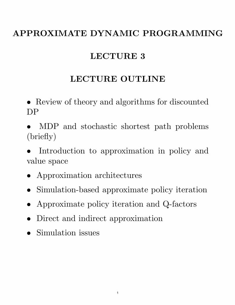
APPROXIMATE DYNAMIC PROGRAMMIN

LECTURE 3

LECTURE OUTLINE

• Review of theory and algorithms for discountedDP

• MDP and stochastic shortest path problems(briefly)

• Introduction to approximation in policy andvalue space

• Approximation architectures

• Simulation-based approximate policy iteration

• Approximate policy iteration and Q-factors

• Direct and indirect approximation

• Simulation issues

G

1

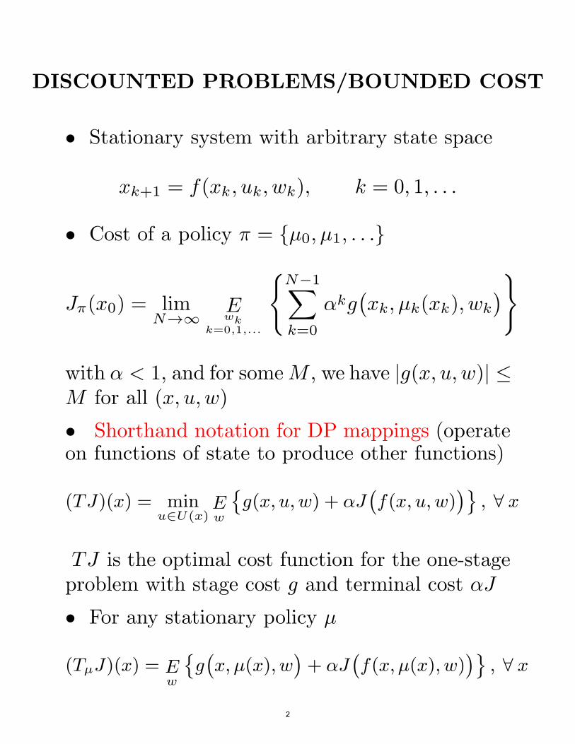
DISCOUNTED PROBLEMS/BOUNDED COST

• Stationary system with arbitrary state space

xk+1 = f(xk, uk, wk), k = 0, 1, . . .

• Cost of a policy ! = {µ0, µ1, . . .}

N!1

J k!(x0) = lim E " g xk, µk(xk), wk

N$% wkk=0,1,...

!

k

"

=0

#

$ %

with " < 1, and for someM , we have |g(x, u, w)| #M for all (x, u, w)

• Shorthand notation for DP mappings (operateon functions of state to produce other functions)

(TJ)(x) = min E g(x, u, w) + !J f(x, u, w) , ! xu!U(x) w

& $ %'

TJ is the optimal cost function for the one-stageproblem with stage cost g and terminal cost "J

• For any stationary policy µ

(TµJ)(x) = E g x, µ(x), w + !J f(x, µ(x), w) , ! xw

& $ % $ %'

2

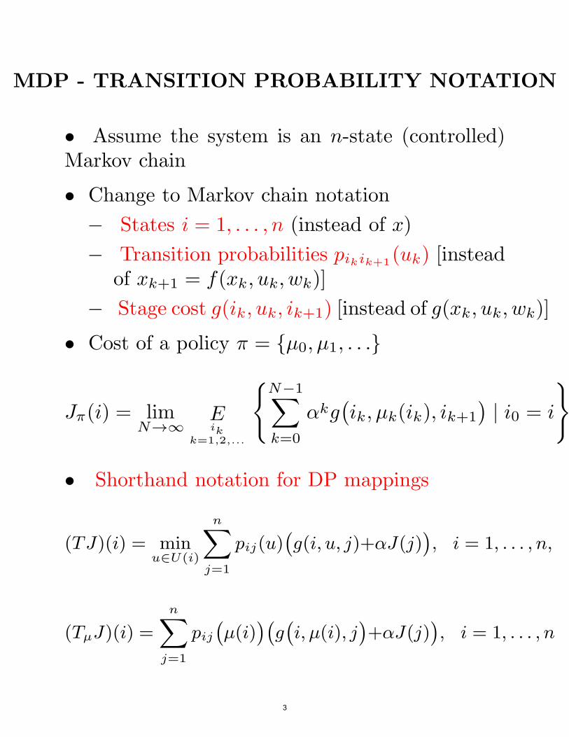
MDP - TRANSITION PROBABILITY NOTATION

• Assume the system is an n-state (controlled)Markov chain

• Change to Markov chain notation

! States i = 1, . . . , n (instead of x)

! Transition probabilities pikik+1(uk) [insteadof xk+1 = f(xk, uk, wk)]

! Stage cost g(ik, uk, ik+1) [instead of g(xk, uk, wk)]

• Cost of a policy ! = {µ0, µ1, . . .}!

N!1

J!(i) = lim E"

"kg$

ik, µk(ik), ik+1

%

| i0 = iN$% ik

k=1,2,... k=0

• Shorthand notation for DP mappings

n

(TJ)(i) = min"

pij(u)$

g(i, u, j)+!J(j)%

, i = 1, . . . , n,u!U(i)

j=1

n

(TµJ)(i) ="

pij$

µ(i)%$

g$

i, µ(i), jj=1

%

+!J(j)%

, i = 1, . . . , n

#

3

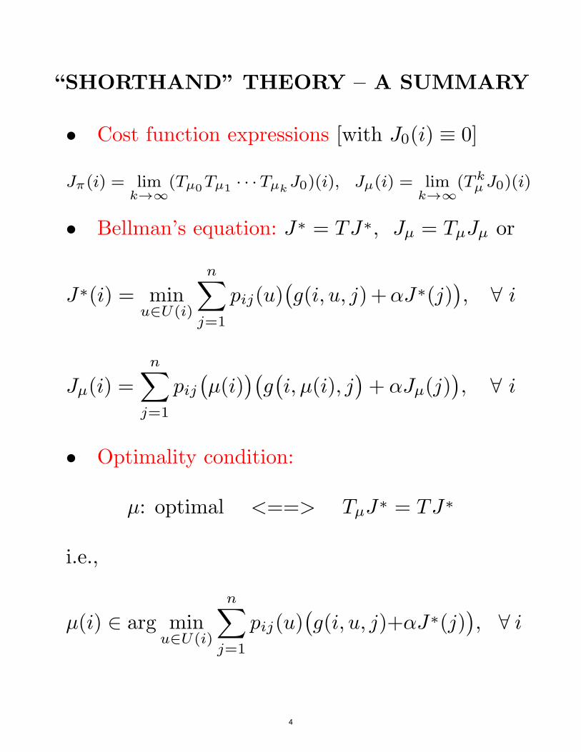
“SHORTHAND” THEORY – A SUMMARY

• Cost function expressions [with J0(i) % 0]

J!(i) = lim (T T kµ0 µ · · ·1 Tµk

J0)(i), Jµ(i) = lim (TµJ0)(i)k"# k"#

• Bellman’s equation: J" = TJ", Jµ = TµJµ or

n

J"(i) = minu#U(i)

"

p (u)$

g(i, u, j)+"J"ij (j)

j=1

%

, $ i

n

Jµ(i) ="

pij µ(i) g i, µ(i), j + "Jµ(j) , ij=1

$ %$ $ % %

$

• Optimality condition:

µ: optimal <==> TµJ" = TJ"

i.e.,

n

µ(i) " arg min"

pij(u) g(i, u, j)+"J"(j) ,u#U(i)

j=1

$ i$ %

4

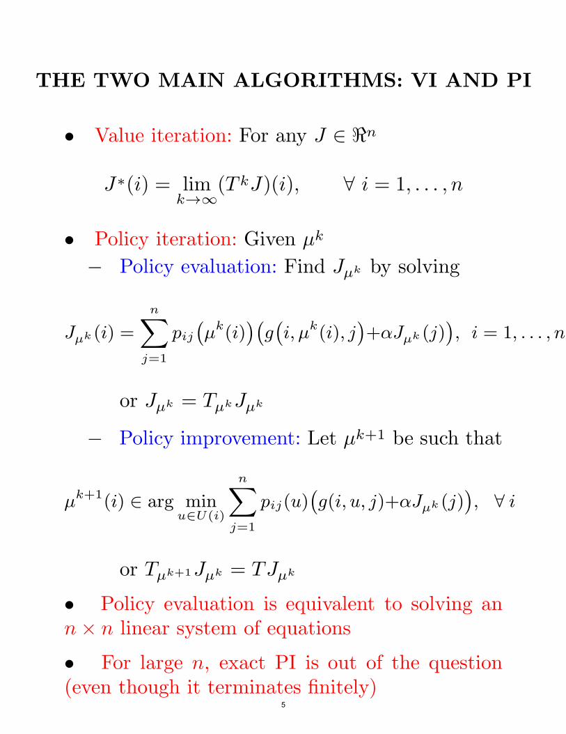
THE TWO MAIN ALGORITHMS: VI AND PI

• Value iteration: For any J " ,n

J"(i) = lim (T kJ)(i),k$%

$ i = 1, . . . , n

• Policy iteration: Given µk

! Policy evaluation: Find Jµk by solving

n

Jµk (i) ="

p k kij

$

µ (i)%$

g$

i, µ (i), j%

+!Jµk (j)%

, i = 1, . . . , nj=1

or Jµk = TµkJµk

! Policy improvement: Let µk+1 be such that

n

µk+1(i) " arg min"

pij(u)$

g(i, u, j)+!Jµk (j)u!U(i)

j=1

%

, ! i

or Tµk+1Jµk = TJµk

• Policy evaluation is equivalent to solving ann- n linear system of equations

• For large n, exact PI is out of the question(even though it terminates finitely)

5

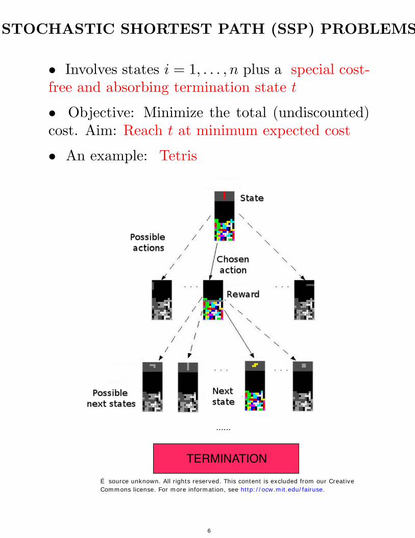
STOCHASTIC SHORTEST PATH (SSP) PROBLEM

• Involves states i = 1, . . . , n plus a special cost-free and absorbing termination state t

• Objective: Minimize the total (undiscounted)cost. Aim: Reach t at minimum expected cost

S

• An example: Tetris

6

É source unknown. All rights reserved. This content is excluded from our CreativeCommons license. For more information, see http://ocw.mit.edu/fairuse.

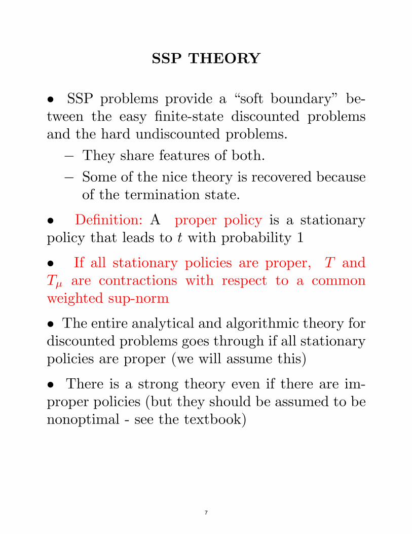
SSP THEORY

• SSP problems provide a “soft boundary” be-tween the easy finite-state discounted problemsand the hard undiscounted problems.

! They share features of both.

! Some of the nice theory is recovered becauseof the termination state.

• Definition: A proper policy is a stationarypolicy that leads to t with probability 1

• If all stationary policies are proper, T andTµ are contractions with respect to a commonweighted sup-norm

• The entire analytical and algorithmic theory fordiscounted problems goes through if all stationarypolicies are proper (we will assume this)

• There is a strong theory even if there are im-proper policies (but they should be assumed to benonoptimal - see the textbook)

7

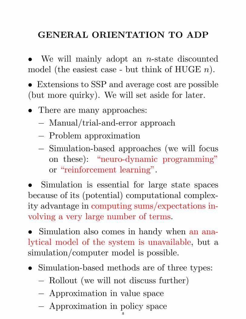
GENERAL ORIENTATION TO ADP

• We will mainly adopt an n-state discountedmodel (the easiest case - but think of HUGE n).

• Extensions to SSP and average cost are possible(but more quirky). We will set aside for later.

• There are many approaches:

! Manual/trial-and-error approach

! Problem approximation

! Simulation-based approaches (we will focuson these): “neuro-dynamic programming”or “reinforcement learning”.

• Simulation is essential for large state spacesbecause of its (potential) computational complex-ity advantage in computing sums/expectations in-volving a very large number of terms.

• Simulation also comes in handy when an ana-lytical model of the system is unavailable, but asimulation/computer model is possible.

• Simulation-based methods are of three types:

! Rollout (we will not discuss further)

! Approximation in value space

Approximation in policy space!8

APPROXIMATION IN VALUE SPACE

• Approximate J" or Jµ from a parametric classJ(i, r) where i is the current state and r = (r1, . . . , rmis a vector of “tunable” scalars weights.

• By adjusting r we can change the “shape” of Jso that it is reasonably close to the true optimalJ".

• Two key issues:

! The choice of parametric class J(i, r) (theapproximation architecture).

! Method for tuning the weights (“training”the architecture).

• Successful application strongly depends on howthese issues are handled, and on insight about theproblem.

• A simulator may be used, particularly whenthere is no mathematical model of the system (butthere is a computer model).

• We will focus on simulation, but this is not theonly possibility [e.g., J(i, r) may be a lower boundapproximation based on relaxation, or other prob-lem approximation]

)

9

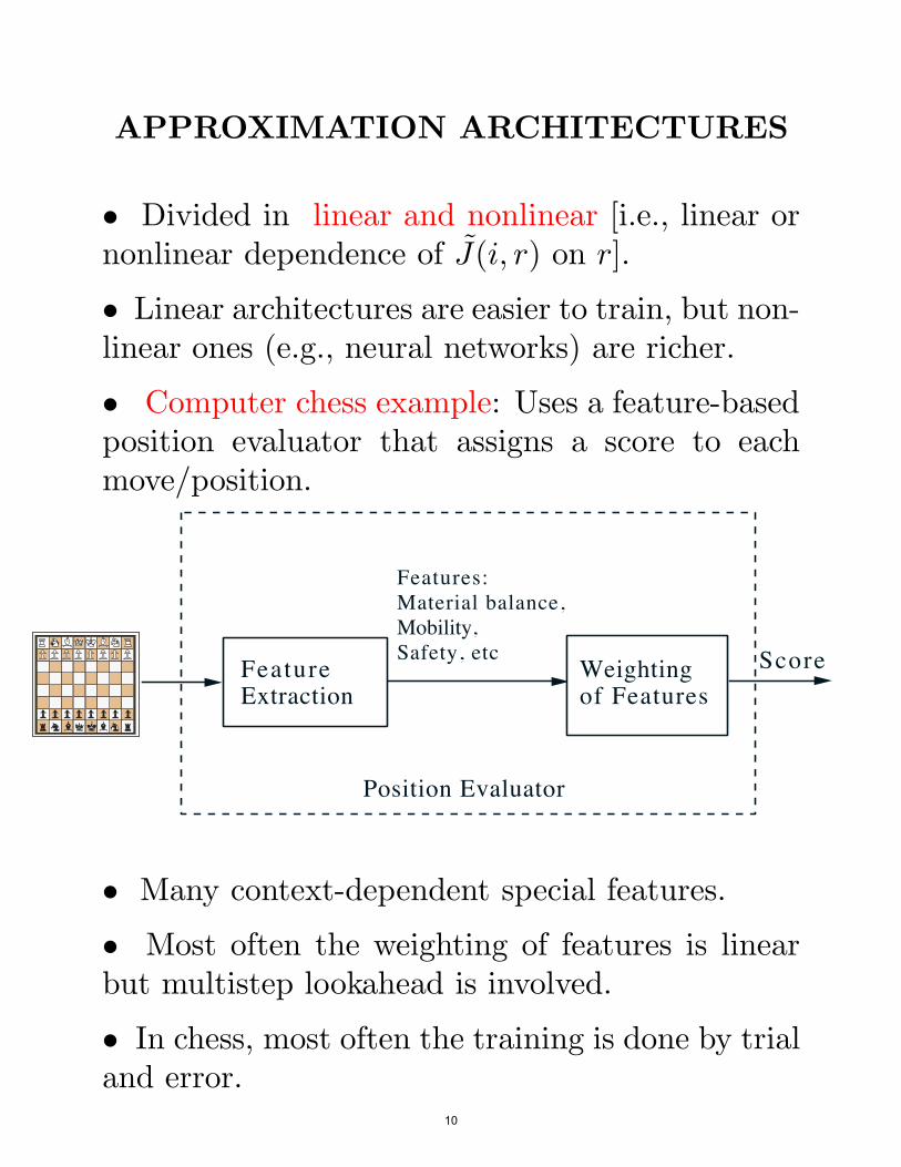
APPROXIMATION ARCHITECTURES

• Divided in linear and nonlinear [i.e., linear ornonlinear dependence of J(i, r) on r].

• Linear architectures are easier to train, but non-linear ones (e.g., neural networks) are richer.

• Computer chess example: Uses a feature-basedposition evaluator that assigns a score to eachmove/position.

Features:Material balance,Mobility,Safety, etc

Feature Weighting ScoreExtraction of Features

Position Evaluator

• Many context-dependent special features.

• Most often the weighting of features is linearbut multistep lookahead is involved.

• In chess, most often the training is done by trialand error.

10

FeatureExtraction

Weightingof Features

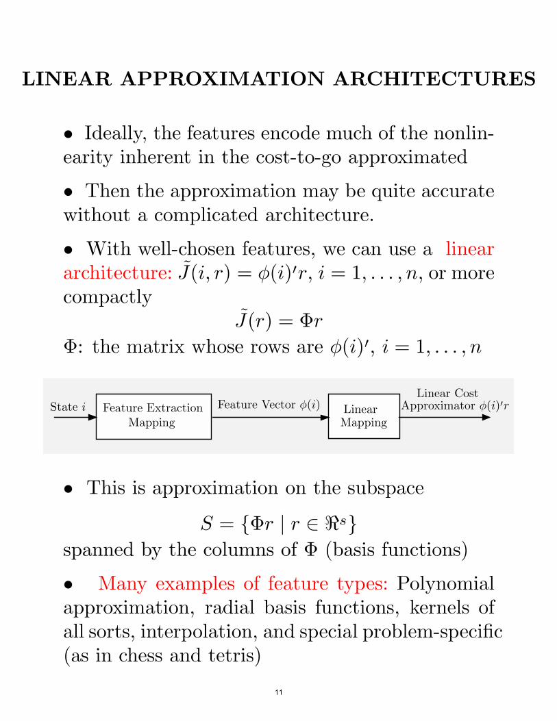
LINEAR APPROXIMATION ARCHITECTURES

• Ideally, the features encode much of the nonlin-earity inherent in the cost-to-go approximated

• Then the approximation may be quite accuratewithout a complicated architecture.

• With well-chosen features, we can use a lineararchitecture: J(i, r) = ((i)&r, i = 1, . . . , n, or morecompactly

J(r) = $r$: the matrix whose rows are ((i)&, i = 1, . . . , n

• This is approximation on the subspace

S = {$r | r " ,s}spanned by the columns of $ (basis functions)

• Many examples of feature types: Polynomialapproximation, radial basis functions, kernels ofall sorts, interpolation, and special problem-specific(as in chess and tetris)

Feature Extraction Mapping Feature VectorApproximator

i Mapping Feature VectorApproximator ( )Feature Extraction Feature VectorFeature Extraction Feature Vector

Feature Extraction Mapping Linear Costi) Cost

i)

11

State i Feature Extraction Mapping Feature VectorApproximator

i Feature Extraction Mapping Feature VectorApproximator ( )Feature Extraction Mapping Feature VectorFeature Extraction Mapping Feature Vector

Feature Extraction Mapping Feature Vector !(i) Linear Costi) Linear Cost

i) Linear CostApproximator !(i)!r

APPROXIMATION IN POLICY SPACE

• A brief discussion; we will return to it at theend.

• We parameterize the set of policies by a vectorr = (r1, . . . , rs) and we optimize the cost over r

• Discounted problem example:

! Each value of r defines a stationary policy,with cost starting at state i denoted by J(i; r).

! Use a random search, gradient, or other methodto minimize over r

n

J(r) ="

piJ(i; r),i=1

where (p1, . . . , pn) is some probability distri-bution over the states.

• In a special case of this approach, the param-eterization of the policies is indirect, through anapproximate cost function.

! A cost approximation architecture parame-terized by r, defines a policy dependent on rvia the minimization in Bellman’s equation.

12

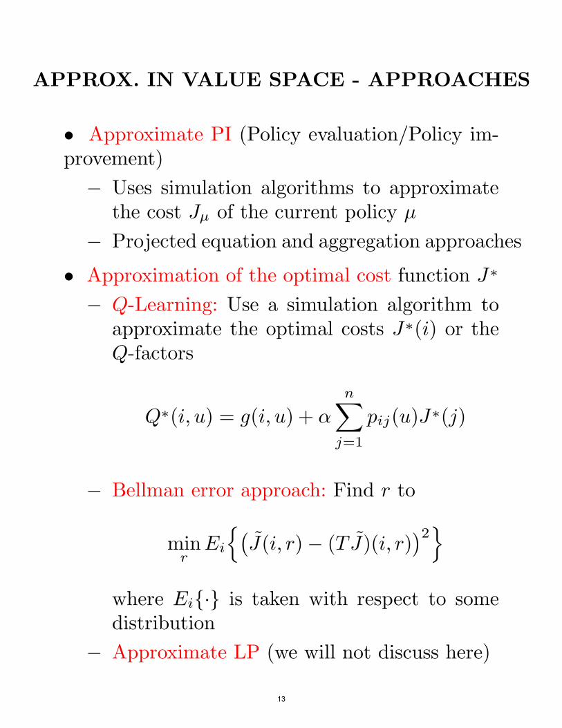
APPROX. IN VALUE SPACE - APPROACHES

• Approximate PI (Policy evaluation/Policy im-provement)

! Uses simulation algorithms to approximatethe cost Jµ of the current policy µ

! Projected equation and aggregation approaches

• Approximation of the optimal cost function J"

! Q-Learning: Use a simulation algorithm toapproximate the optimal costs J"(i) or theQ-factors

n

Q"(i, u) = g(i, u) + ""

pij(u)J"(j)j=1

! Bellman error approach: Find r to

2minEi

(

$

J(i, r)! (T J)(i, r)r

%

)

where Ei{·} is taken with respect to somedistribution

! Approximate LP (we will not discuss here)

13

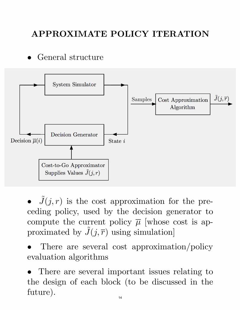
APPROXIMATE POLICY ITERATION

• General structure

System Simulator

Decision Generator) Decision µ(i) S

Cost-to-Go Approximatorn Generatorr Supplies Values J(j, r) D

Cost Approximationn Algorithm

J(j, r)

State i

) Samples

DCost-to-Go Approx

rroximator Supplies Valur

SState Cost Approximation

ecisio

i A

C

r

• J(j, r) is the cost approximation for the pre-ceding policy, used by the decision generator tocompute the current policy µ [whose cost is ap-proximated by J(j, r) using simulation]

• There are several cost approximation/policyevaluation algorithms

• There are several important issues relating tothe design of each block (to be discussed in the

˜

future).14

r) Samples

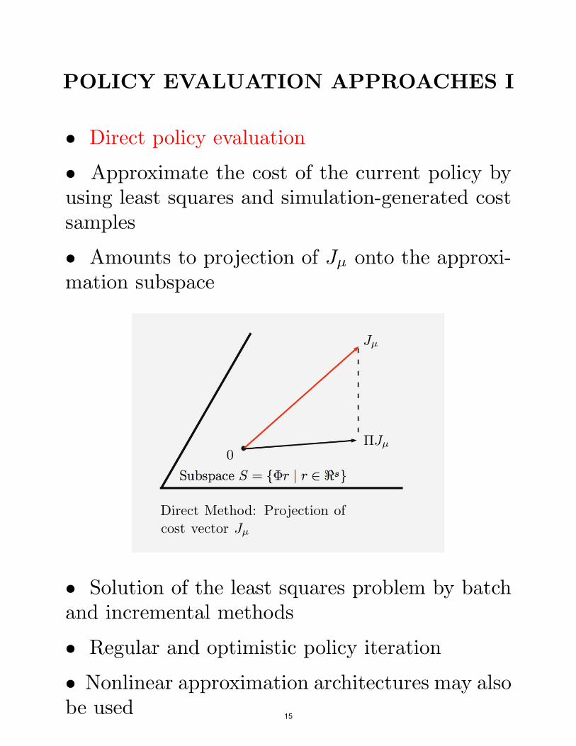
POLICY EVALUATION APPROACHES I

• Direct policy evaluation

• Approximate the cost of the current policy byusing least squares and simulation-generated costsamples

• Amounts to projection of Jµ onto the approxi-mation subspace

Subspace S = {!r | r ! "s}

Jµ

!Jµ

Direct Method: Projection ofcost vector Jµ

Set

Direct Method: Projection of cost vector !

µ

cost vectorDirect Method: Projection of

• Solution of the least squares problem by batchand incremental methods

• Regular and optimistic policy iteration

Nonlinear approximation architectures may also•be used 15

= 0

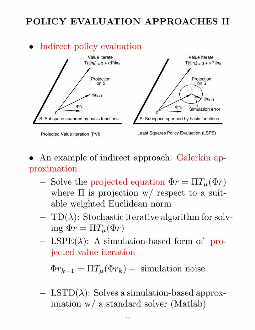
POLICY EVALUATION APPROACHES II

• Indirect policy evaluationValue Iterate Value Iterate

T(Φrk) = g + αPΦrk T(Φrk) = g + αPΦrk

Projection Projectionon S on S

Φrk+1Φrk+1

Φrk Φrk Simulation error0 0

S: Subspace spanned by basis functions S: Subspace spanned by basis functions

Projected Value Iteration (PVI) Least Squares Policy Evaluation (LSPE)

• An example of indirect approach: Galerkin ap-proximation

! Solve the projected equation $r = #Tµ($r)where # is projection w/ respect to a suit-able weighted Euclidean norm

! TD()): Stochastic iterative algorithm for solv-ing $r = #Tµ($r)

! LSPE()): A simulation-based form of pro-jected value iteration

$rk+1 = #Tµ($rk) + simulation noise

! LSTD()): Solves a simulation-based approx-imation w/ a standard solver (Matlab)

16

POLICY EVALUATION APPROACHES III

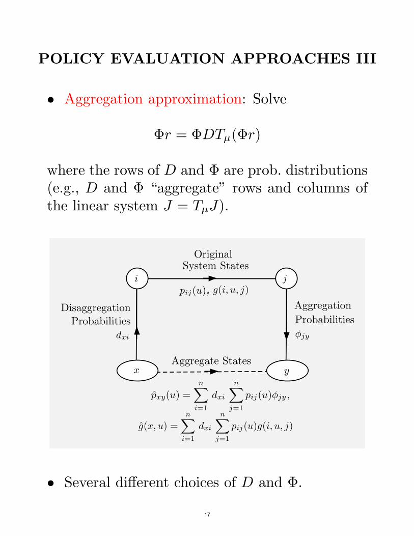
• Aggregation approximation: Solve

$r = $DTµ($r)

where the rows of D and $ are prob. distributions(e.g., D and $ “aggregate” rows and columns ofthe linear system J = TµJ).

pij(u),

dxi !jy

i

x y

OriginalSystem States

Aggregate States

pxy(u) =n!

i=1

dxi

n!

j=1

pij(u)!jy ,

Disaggregation

Probabilities

Aggregation

Probabilities

g(x, u) =n!

i=1

dxi

n!

j=1

pij(u)g(i, u, j)

, g(i, u, j)according to with cost

S

= 1

), ),

System States Aggregate States

!

Original Aggregate States

!

|

Original System States

Probabilities

!

AggregationDisaggregation Probabilities

ProbabilitiesDisaggregation Probabilities

!

AggregationDisaggregation Probabilities

Matrix

• Several di!erent choices of D and $.

17

, j = 1

POLICY EVALUATION APPROACHES IV

pij(u),

dxi !jy

i

x y

OriginalSystem States

Aggregate States

pxy(u) =n!

i=1

dxi

n!

j=1

pij(u)!jy ,

Disaggregation

Probabilities

Aggregation

Probabilities

g(x, u) =n!

i=1

dxi

n!

j=1

pij(u)g(i, u, j)

, g(i, u, j)according to with cost

S

= 1

), ),

System States Aggregate States

!

Original Aggregate States

!

|

Original System States

Probabilities

!

AggregationDisaggregation Probabilities

ProbabilitiesDisaggregation Probabilities

!

AggregationDisaggregation Probabilities

Matrix

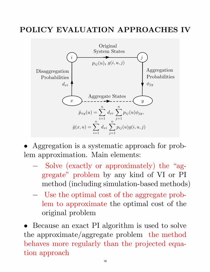
• Aggregation is a systematic approach for prob-lem approximation. Main elements:

! Solve (exactly or approximately) the “ag-gregate” problem by any kind of VI or PImethod (including simulation-based methods)

! Use the optimal cost of the aggregate prob-lem to approximate the optimal cost of theoriginal problem

• Because an exact PI algorithm is used to solvethe approximate/aggregate problem the methodbehaves more regularly than the projected equa-tion approach

18

, j = 1

THEORETICAL BASIS OF APPROXIMATE PI

• If policies are approximately evaluated using anapproximation architecture such that

max |J(i, rk)! Jµk(i)i

| # #, k = 0, 1, . . .

• If policy improvement is also approximate,

max |(Tµk+1 J)(i, rk) (i

! T J)(i, rk)| # $, k = 0, 1, . . .

• Error bound: The sequence {µk} generated byapproximate policy iteration satisfies

$+ 2"#lim supmax

$

Jµk(i)ik$%

! J"(i)%

#(1! ")2

• Typical practical behavior: The method makessteady progress up to a point and then the iteratesJµk oscillate within a neighborhood of J".

19

THE USE OF SIMULATION - AN EXAMPLE

• Projection by Monte Carlo Simulation: Com-pute the projection# J of a vector J " ,n onsubspace S = {$r | r " ,s}, with respect to aweighted Euclidean norm ) · )&.

• Equivalently, find$ r", wheren

2r" = arg min )$r!J)2 = arg min

"

*$

((i)&i& r (i#'s r#'

i=1

!J )r s

• Setting to 0 the gradient at r",

%

r" =

0 !1n n"

*i((i)((i)&

i=1

1

"

*i((i)J(i)i=1

• Approximate by simulation the two “expectedvalues”

rk =

0 !1k k"

((i (i &t)( t)

t=1

1

"

((it)J(it)t=1

• Equivalent least squares alternative:k

2rk = arg min ((it)&r J(it)

r#'s!

"

t=1

$ %

20

THE ISSUE OF EXPLORATION

• To evaluate a policy µ, we need to generate costsamples using that policy - this biases the simula-tion by underrepresenting states that are unlikelyto occur under µ.

• As a result, the cost-to-go estimates of theseunderrepresented states may be highly inaccurate.

• This seriously impacts the improved policy µ.

• This is known as inadequate exploration - aparticularly acute di"culty when the randomnessembodied in the transition probabilities is “rela-tively small” (e.g., a deterministic system).

• One possibility for adequate exploration: Fre-quently restart the simulation and ensure that theinitial states employed form a rich and represen-tative subset.

• Another possibility: Occasionally generate tran-sitions that use a randomly selected control ratherthan the one dictated by the policy µ.

• Other methods, to be discussed later, use twoMarkov chains (one is the chain of the policy andis used to generate the transition sequence, theother is used to generate the state sequence).

21

APPROXIMATING Q-FACTORS

• The approach described so far for policy eval-uation requires calculating expected values [andknowledge of pij(u)] for all controls u " U(i).

• Model-free alternative: Approximate Q-factors

n

Q(i, u, r) *"

pij(u)j=1

$

g(i, u, j) + "Jµ(j)%

and use for policy improvement the minimization

µ(i) = arg min Q(i, u, r)u#U(i)

• r is an adjustable parameter vector and Q(i, u, r)is a parametric architecture, such as

s

Q(i, u, r) ="

rm(m(i, u)m=1

• We can use any approach for cost approxima-tion, e.g., projected equations, aggregation.

• Use the Markov chain with states (i, u) - pij(µ(i))is the transition prob. to (j, µ(i)), 0 to other (j, u&).

Major concern: Acutely diminished exploration.•22

MIT OpenCourseWarehttp://ocw.mit.edu

6.231 Dynamic Programming and Stochastic ControlFall 2015

For information about citing these materials or our Terms of Use, visit: http://ocw.mit.edu/terms.