Approximate k- at Nearest Neighbor Search

Approximate k-�at Nearest Neighbor Search∗

Wolfgang Mulzer† Huy L. Nguy�ên‡ Paul Seiferth† Yannik Stein†

Abstract

Let k be a nonnegative integer. In the approximate k-�at nearest neighbor (k-ANN) problem, we aregiven a set P ⊂ Rd of n points in d-dimensional space and a �xed approximation factor c > 1. Our goalis to preprocess P so that we can e�ciently answer approximate k-�at nearest neighbor queries: givena k-�at F , �nd a point in P whose distance to F is within a factor c of the distance between F andthe closest point in P . The case k = 0 corresponds to the well-studied approximate nearest neighborproblem, for which a plethora of results are known, both in low and high dimensions. The case k = 1 iscalled approximate line nearest neighbor. In this case, we are aware of only one provably e�cient datastructure, due to Andoni, Indyk, Krauthgamer, and Nguy�ên (AIKN) [2]. For k ≥ 2, we know of noprevious results.

We present the �rst e�cient data structure that can handle approximate nearest neighbor queries forarbitrary k. We use a data structure for 0-ANN-queries as a black box, and the performance depends onthe parameters of the 0-ANN solution: suppose we have an 0-ANN structure with query time O(nρ) andspace requirement O(n1+σ), for ρ, σ > 0. Then we can answer k-ANN queries in time O(nk/(k+1−ρ)+t)

and space O(n1+σk/(k+1−ρ) + n logO(1/t) n). Here, t > 0 is an arbitrary constant and the O-notationhides exponential factors in k, 1/t, and c and polynomials in d.

Our approach generalizes the techniques of AIKN for 1-ANN: we partition P into clusters of increas-ing radius, and we build a low-dimensional data structure for a random projection of P . Given a query�at F , the query can be answered directly in clusters whose radius is �small� compared to d(F, P ) usinga grid. For the remaining points, the low dimensional approximation turns out to be precise enough.Our new data structures also give an improvement in the space requirement over the previous resultfor 1-ANN: we can achieve near-linear space and sublinear query time, a further step towards practicalapplications where space constitutes the bottleneck.

∗WM and PS were supported in part by DFG Grants MU 3501/1 and MU 3501/2. YS was supported by theDeutsche Forschungsgemeinschaft within the research training group `Methods for Discrete Structures' (GRK1408).†Institut für Informatik, Freie Universität Berlin, {mulzer,pseiferth,yannikstein}@inf.fu-berlin.de.‡Simons Institute, UC Berkeley [email protected].

1

1 Introduction 1

1 Introduction

Nearest neighbor search is a fundamental problem in computational geometry, with countlessapplications in databases, information retrieval, computer vision, machine learning, signal pro-cessing, etc. [10]. Given a set P ⊂ Rd of n points in d-dimensional space, we would like topreprocess P so that for any query point q ∈ Rd, we can quickly �nd the point in P that isclosest to q.

There are e�cient algorithms if the dimension d is �small� [7, 18]. However, as d increases,these algorithms quickly become ine�cient: either the query time approaches linear or the spacegrows exponentially with d. This phenomenon is usually called the �curse of dimensionality�.Nonetheless, if one is satis�ed with just an approximate nearest neighbor whose distance to thequery point q lies within some factor c = 1 + ε, ε > 0, of the distance between q and the actualnearest neighbor, there are e�cient solutions even for high dimensions. Several methods areknown, o�ering trade-o�s between the approximation factor, the space requirement, and thequery time (see, e.g., [1, 3] and the references therein).

From a practical perspective, it is important to keep both the query time and the spacesmall. Ideally, we would like algorithms with almost linear (or at least sub-quadratic) spacerequirement and sub-linear query time. Fortunately, there are solutions with these guarantees.These methods include locality sensitive hashing (LSH) [11,12] and a more recent approach thatimproves upon LSH [3]. Speci�cally, the latter algorithm achieves query time n7/(8c2)+O(1/c3)

and space n1+7/(8c2)+O(1/c3), where c is the approximation factor.Often, however, the query object is more complex than a single point. Here, the complexity

of the problem is much less understood. Perhaps the simplest such scenario occurs when thequery object is a k-dimensional �at, for some small constant k. This is called the approximate k-�at nearest neighbor problem [2]. It constitutes a natural generalization of approximate nearestneighbors, which corresponds to k = 0. In practice, low-dimensional �ats are used to modeldata subject to linear variations. For example, one could capture the appearance of a physicalobject under di�erent lighting conditions or under di�erent viewpoints (see [4] and the referencestherein).

So far, the only known algorithm with worst-case guarantees is for k = 1, the approximateline nearest neighbor problem. For this case, Andoni, Indyk, Krauthgamer, and Nguy�ên (AIKN)achieve sub-linear query time dO(1)n1/2+t and space dO(1)nO(1/ε2+1/t2), for arbitrarily small t > 0.For the �dual� version of the problem, where the query is a point but the data set consists ofk-�ats, three results are known [4,14,15]. The �rst algorithm is essentially a heuristic with somecontrol of the quality of approximation [4]. The second algorithm provides provable guaranteesand a very fast query time of (d + log n + 1/ε)O(1) [14]. The third result, due to Mahabadi,is very recent and improves the space requirement of Magen's result [15]. Unfortunately, thesealgorithms all su�er from very high space requirements, thus limiting their applicability inpractice. In fact, even the basic LSH approach for k = 0 is already too expensive for largedatasets and additional theoretical work and heuristics are required to reduce the memory usageand make LSH suitable for this setting [13, 19]. For k ≥ 2, we know of no results in the theoryliterature.Our results. We present the �rst e�cient data structure for general approximate k-�at nearestneighbor search. Suppose we have a data structure for approximate point nearest neighborsearch with query time O(nρ+d log n) and space O(n1+σ +d log n), for some constants ρ, σ > 0.Then our algorithm achieves query time O(dO(1)nk/(k+1−ρ)+t) and space O(dO(1)n1+σk/(k+1−ρ) +n logO(1/t) n), where t > 0 can be made arbitrarily small. The constant factors for the querytime depend on k, c, and 1/t. Our main result is as follows.

Theorem 1.1. Fix an integer k ≥ 1 and an approximation factor c > 1. Suppose we have a datastructure for approximate point nearest neighbor search with query time O(nρ+d log n) and spaceO(n1+σ + d log n), for some constants ρ, σ > 0. Let P ⊂ Rd be a d-dimensional n-point set. For

2 Main Data Structure and Algorithm Overview 2

any parameter t > 0, we can construct a data structure with O(dO(1)n1+kσ/(k+1−ρ)+n logO(1/t) n)space that can answer the following queries in expected time O(dO(1)nk/(k+1−ρ)+t): given a k-�atF ⊂ Rd, �nd a point p ∈ P with d(p, F ) ≤ cd(P, F ).

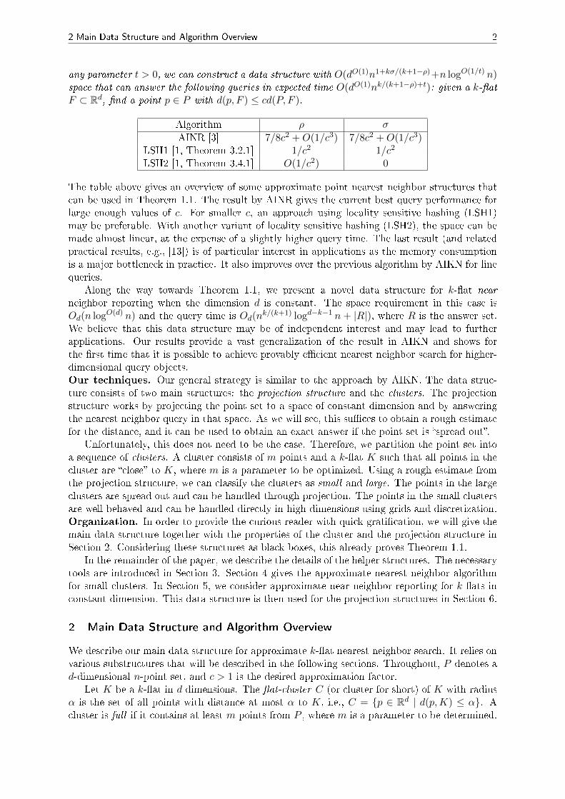
Algorithm ρ σ

AINR [3] 7/8c2 +O(1/c3) 7/8c2 +O(1/c3)LSH1 [1, Theorem 3.2.1] 1/c2 1/c2

LSH2 [1, Theorem 3.4.1] O(1/c2) 0

The table above gives an overview of some approximate point nearest neighbor structures thatcan be used in Theorem 1.1. The result by AINR gives the current best query performance forlarge enough values of c. For smaller c, an approach using locality sensitive hashing (LSH1)may be preferable. With another variant of locality sensitive hashing (LSH2), the space can bemade almost linear, at the expense of a slightly higher query time. The last result (and relatedpractical results, e.g., [13]) is of particular interest in applications as the memory consumptionis a major bottleneck in practice. It also improves over the previous algorithm by AIKN for linequeries.

Along the way towards Theorem 1.1, we present a novel data structure for k-�at nearneighbor reporting when the dimension d is constant. The space requirement in this case isOd(n logO(d) n) and the query time is Od(n

k/(k+1) logd−k−1 n+ |R|), where R is the answer set.We believe that this data structure may be of independent interest and may lead to furtherapplications. Our results provide a vast generalization of the result in AIKN and shows forthe �rst time that it is possible to achieve provably e�cient nearest neighbor search for higher-dimensional query objects.Our techniques. Our general strategy is similar to the approach by AIKN. The data struc-ture consists of two main structures: the projection structure and the clusters. The projectionstructure works by projecting the point set to a space of constant dimension and by answeringthe nearest neighbor query in that space. As we will see, this su�ces to obtain a rough estimatefor the distance, and it can be used to obtain an exact answer if the point set is �spread out�.

Unfortunately, this does not need to be the case. Therefore, we partition the point set intoa sequence of clusters. A cluster consists of m points and a k-�at K such that all points in thecluster are �close� to K, where m is a parameter to be optimized. Using a rough estimate fromthe projection structure, we can classify the clusters as small and large. The points in the largeclusters are spread out and can be handled through projection. The points in the small clustersare well behaved and can be handled directly in high dimensions using grids and discretization.Organization. In order to provide the curious reader with quick grati�cation, we will give themain data structure together with the properties of the cluster and the projection structure inSection 2. Considering these structures as black boxes, this already proves Theorem 1.1.

In the remainder of the paper, we describe the details of the helper structures. The necessarytools are introduced in Section 3. Section 4 gives the approximate nearest neighbor algorithmfor small clusters. In Section 5, we consider approximate near neighbor reporting for k-�ats inconstant dimension. This data structure is then used for the projection structures in Section 6.

2 Main Data Structure and Algorithm Overview

We describe our main data structure for approximate k-�at nearest neighbor search. It relies onvarious substructures that will be described in the following sections. Throughout, P denotes ad-dimensional n-point set, and c > 1 is the desired approximation factor.

Let K be a k-�at in d dimensions. The �at-cluster C (or cluster for short) of K with radiusα is the set of all points with distance at most α to K, i.e., C = {p ∈ Rd | d(p,K) ≤ α}. Acluster is full if it contains at least m points from P , where m is a parameter to be determined.


We call P α-cluster-free if there is no full cluster with radius α. Let t > 0 be an arbitrarilysmall parameter. Our data structure requires the following three subqueries.

Q1: Given a query �at F , �nd a point p ∈ P with d(p, F ) ≤ ntd(P, F ).

Q2: Assume P is contained in a �at-cluster with radius α. Given a query �at F with d(P, F ) ≥α/n2t, return a point p ∈ P with d(p, F ) ≤ cd(P, F ).

Q3: Assume P is αn2t/(2k + 1)-cluster free. Given a query �at F with d(P, F ) ≤ α, �nd thenearest neighbor p∗ ∈ P to F .

Brie�y, our strategy is as follows: during the preprocessing phase, we partition the point setinto a set of full clusters of increasing radii. To answer a query F , we �rst perform a query oftype Q1 to obtain an nt-approximate estimate r for d(P, F ). Using r, we identify the �small�clusters. These clusters can be processed using a query of type Q2. The remaining point setcontains no �small� full cluster, so we can process it with a query of type Q3.

We will now describe the properties of the subqueries and the organization of the datastructure in more detail. The data structure for Q2-queries is called the cluster structure. It isdescribed in Section 4, and it has the following properties.

Theorem 2.1. Let Q be a d-dimensional m-point set that is contained in a �at-cluster of radiusα. Let c > 1 be an approximation factor. Using space Oc(m

1+σ + d log2m), we can build adata structure with the following property. Given a query k-�at F with d(P, F ) ≥ α/n2t and anestimate r with d(P, F ) ∈ [r/nt, r], we can �nd a c-approximate nearest neighbor for F in Q intotal time Oc((n

2tk2)k+1(m1−1/k+ρ/k + (d/k) logm)).

The data structures for Q1 and Q3 are very similar, and we cover them in Section 6. Theyare called projection structures, since they are based on projecting P into a low dimensionalsubspace. In the projected space, we use a data structure for approximate k-�at near neighborsearch to be described in Section 5. The projection structures have the following properties.

Theorem 2.2. Let P be a d-dimensional n-point set, and let t > 0 be a small enough con-stant. Using space and time O(n logO(1/t) n), we can obtain a data structure for the follow-ing query: given a k-�at F , �nd a point p ∈ P with d(p, F ) ≤ ntd(P, F ). A query needsO(nk/(k+1) logO(1/t) n) time, and the answer is correct with high probability.

Theorem 2.3. Let P be a d-dimensional n-point set, and let t > 0 be a small enough constant.Using space and time O(n logO(1/t) n), we can obtain a data structure for the following query:given a k-�at F and α > 0 such that d(F, P ) ≤ α and such that P is αnt/(2k + 1)-cluster-free,�nd an exact nearest neighbor for F in P . A query needs O(nk/(k+1) logO(1/t) n+m) time, andthe answer is correct with high probability. Here, m denotes the size of a full cluster.

2.1 Constructing the Data Structure

First, we build a projection structure for Q1 queries on P . This needs O(n logO(1/t) n) space,by Theorem 2.2. Then, we repeatedly �nd the full �at-cluster C with smallest radius. The mpoints in C are removed from P , and we build a cluster structure for Q2 queries on this set. ByTheorem 2.1, this needs Oc(m

1+σ + d log2m) space. To �nd C, we check all �ats K spannedby k + 1 distinct points of P . In Lemma 3.2 below, we prove that this provides a good enoughapproximation. In the end, we have n/m point sets Q1, . . . , Qn/m ordered by decreasing radius,i.e., the cluster for Q1 has the largest radius. The total space occupied by the cluster structuresis O(nmσ + (n/m)d log2 n).

Finally, we build a perfect binary tree T with n/m leaves labeled Q1, . . . , Qn/m, from leftto right. For a node v ∈ T let Qv be the union of all Qi assigned to leaves below v. For eachv ∈ T we build a data structure for Qv to answer Q3 queries. Since each point is contained inO(log n) data structures, the total size is O(n logO(1/t) n), by Theorem 2.3. For pseudocode, seeAlgorithm 1.


Input: point set P ⊂ Rd, approximation factor c, parameter t > 01 Q← P2 for i← n/m downto 1 do

3 For each V ∈(Qk+1

), consider the k-�at KV de�ned by V . Let αV be the radius of the

smallest �at-cluster of KV with exactly m points of Q.4 Choose the �at K = KV that minimizes αV and set αi = αV .5 Remove from Q the set Qi of m points in Q within distance αi from K.6 Construct a cluster structure Ci for the cluster (K,Qi).

7 Build a perfect binary tree T with n/m leaves, labeled Q1, . . . , Qn/m from left to right.

8 foreach node v ∈ T do

9 Build data structure for Q3 queries as in Theorem 2.3 for the set Qv corresponding tothe leaves below v.

Algorithm 1: Preprocessing algorithm. Compared with AIKN [2], we organize the pro-jection structure in a tree to save space.

2.2 Performing a Query

Suppose we are given a k-�at F . To �nd an approximate nearest neighbor for F we proceedsimilarly as AIKN [2]. We use Q2 queries on �small� clusters and Q3 queries on the remainingpoints; for pseudocode, see Algorithm 2.

Input : query �at FOutput: a c-approximate nearest neighbor for F in P

1 Query the root of T for a nt-approximate nearest neighbor p1 to F . /* type Q1 */

2 r ← d(p1, F )3 i∗ ← maximum i ∈ {1, . . . , n/m} with αi > rnt, or 0 if no such i exists4 for i← i∗ + 1 to n/m do

/* type Q2; we have d(Qi, F ) ≥ r/nt ≥ αi/n2t */

5 Query cluster structure Ci with estimate r.

/* type Q3 */

6 Query projection structure for a r-thresholded nearest neighbor of F in Q =⋃j∗

i=1 Ui.return closest point to F among query results.

Algorithm 2: Algorithm for �nding approximate nearest neighbor in high dimensions.

First, we perform a query of type Q1 to get a nt-approximate nearest neighbor p1 for Fin time O(nk/(k+1) logO(1/t) n). Let r = d(p1, F ). We use r as an estimate to distinguishbetween �small� and �large� clusters. Let i∗ ∈ {1, . . . , n/m} be the largest integer such thatthe cluster assigned with Qi∗ has radius αi∗ > rnt. For i = i∗ + 1, . . . , n/m, we use r as anestimate for a Q2 query on Qi. Since |Qi| = m and by Theorem 2.1, this needs total timeO(n2t(k+1)+1m−1/k+ρ/k + (n/m)d log2m).

It remains to deal with points in �large� clusters. The goal is to perform a type Q3 query on⋃1≤i≤i∗ Qi. For this, we start at the leaf of T labeled Qi∗ and walk up to the root. Each time

we encounter a new node v from its right child, we perform a Q3 query on Qu, where u denotesthe left child of v. Let L be all the left children we �nd in this way. Then clearly we have|L| = O(log n) and

⋃u∈LQu =

⋃1≤i≤i∗ Qi. Moreover, by construction, there is no full cluster

with radius less than rnt de�ned by k + 1 vertices of Qu for any u ∈ L. We will see that thisimplies every Qu to be rn

t/(2k+1)-cluster-free, so Theorem 2.3 guarantees a total query time ofO(nk/(k+1) logO(1/t) n+m) for this step. Among all the points we obtained during the queries,we return the one that is closest to F . A good trade-o� point is achieved for m = nm−1/k+ρ/k,i.e., for m = nk/(k+1−ρ). This gives the bounds claimed in Theorem 1.1.Correctness. Let p∗ be a point with d(p∗, F ) = d(P, F ). First, suppose that p∗ ∈ Qi, for some

3 Preliminaries 5

i > i∗. Then, we have d(p∗, F ) ≥ r/nt ≥ αi/n2t, where αi is the radius of the cluster assigned

to Qi. Since r is a valid nt-approximate estimate for d(F,Qi), a query of type Q2 on Qi givesa c-approximate nearest neighbor, by Theorem 2.1. Now, suppose that p∗ ∈ Qi for 1 ≤ i ≤ i∗.Let u be the node of L with p∗ ∈ Qu. Then Theorem 2.3 guarantees that we will �nd p∗ whendoing a Q3 query on Qu.

3 Preliminaries

Partition Trees. Our algorithm relies on partition trees [6, 16]. We use the optimal versiondue to Chan [5], as summarized in the following theorem.

Theorem 3.1 (Optimal Partition Trees [5]). For any d-dimensional n-point set P ⊂ Rd, andfor any large enough constant r, there is a partition tree T with the following properties: (i) thetree T has degree O(r) and depth logr n; (ii) each node is of the form (Q,∆), where Q is a subsetof P and ∆ a relatively open simplex that contains Q; (iii) for each node (Q,∆), the simplicesof the children of Q are contained in ∆ and are pairwise disjoint; (iv) the point set associatedwith a node of depth ` has size at most n/r`; (v) for any hyperplane h in Rd, the number m` ofsimplices in T that h intersects at level ` obeys the recurrence

m` = O(r`(d−1)/d + r`(d−2)/(d−1)m`−1 + r` log r log n).

Thus, h intersects O(n1−1/d) simplices in total. The tree T can be build in expected timeO(n log n).

k-�at Discretization. For our cluster structure we must �nd k-�ats that are close to manypoints. The following lemma shows that it su�ces to check �few� k-�ats for this.

Lemma 3.2. Let P ⊂ Rd be a �nite point set with |P | ≥ k+1, and let F ⊂ Rd be a k-�at. Thereis a k-�at F ′ such that F ′ is the a�ne hull of k + 1 points in P and δF ′(P ) ≤ (2k + 1)δF (P ),where δF ′(P ) = maxp∈P d(p, F ′) and δF (P ) = maxp∈P d(p, F ).

Proof. This proof generalizes the proof of Lemma 2.3 by AIKN [2].Let Q be the orthogonal projection of P onto F . We may assume that F is the a�ne hull

of Q, since otherwise we could replace F by a�(Q) without a�ecting δF (P ). We choose anorthonormal basis for Rd such that F is the linear subspace spanned by the �rst k coordinates.An a�ne basis for F ′ is constructed as follows: �rst, take a point p0 ∈ P whose x1-coordinateis minimum. Let q0 be the projection of p0 onto F , and translate the coordinate system suchthat q0 is the origin. Next, choose k additional points p1, . . . , pk ∈ P such that |det(q1, . . . , qk)|is maximum, where qi is the projection of pi onto F , for i = 1, . . . , k. That is, we choose kadditional points such that the volume of the k-dimensional parallelogram spanned by theirprojections onto F is maximized. The set {q1, . . . , qk} is a basis for F , since the maximumdeterminant cannot be 0 by our assumption that F is spanned by Q.

Now �x some point p ∈ P and let q be its projection onto F . We write q =∑k

i=1 µiqi. Then,

the point r =∑k

i=1 µipi + (1−∑k

i=1 µi)p0 lies in F ′. By the triangle inequality, we have

d(p, r) ≤ d(p, q) + d(q, r) ≤ δF (P ) + d(q, r). (1)

To upper-bound d(q, r) we �rst show that all coe�cients µi lie in [−1, 1].

Claim 3.3. Take p ∈ P , q ∈ Q and q1, . . . , qk as above. Write q =∑k

i=1 µiqi. Then fori = 1, . . . , k, we have µi ∈ [−1, 1], and µj ≥ 0 for at least one j ∈ {1, . . . , k}.

Proof. We �rst prove that all coe�cients µi lie in the interval [−1, 1]. Suppose that |µi| > 1 forsome i ∈ {1, . . . , k}. We may assume that i = 1. Using the linearity of the determinant,

|det(q, q2, . . . , qk)| = | det(µ1q1, q2, . . . , qk)| = |µ1|·|det(q1, q2, . . . , qk)| > | det(q1, q2, . . . , qk)|,

4 Cluster Structure 6

contradicting the choice of q1, . . . , qk.Furthermore, by our choice of the origin, all points in Q have a non-negative x1-coordinate.

Thus, at least one coe�cient µj , j ∈ {1, . . . , k}, has to be non-negative.

Using Claim 3.3, we can now bound d(q, r). For i = 1, . . . , k, we write pi = qi + q⊥i , whereq⊥i is orthogonal to F . Then,

d(q, r) =

∥∥∥∥∥k∑i=1

µiqi −k∑i=1

µi(qi + q⊥i )−

(1−

k∑i=1

µi

)p0

∥∥∥∥∥=

∥∥∥∥∥k∑i=1

µiq⊥i +

(1−

k∑i=1

µi

)p0

∥∥∥∥∥ ≤(

k∑i=1

|µi|+

∣∣∣∣∣1−k∑i=1

µi

∣∣∣∣∣)δF (P ) ≤ 2kδF (P ), (2)

since ‖q⊥1 ‖, . . . , ‖q⊥k ‖, ‖p0‖ ≤ δF (P ), and since∣∣∣1−∑k

i=1 µi

∣∣∣ ≤ k follows from fact that at least

one µi is non-negative. By (1) and (2), we get d(p, F ′) ≤ (2k + 1)δF (P ).

Remark 3.4. For k = 1, the proof of Lemma 3.2 coincides with the proof of Lemma 2.3 byAIKN [2]. In this case, one can obtain a better bound on d(q, r) since q is a convex combinationof q0 and q1. This gives δF ′(P ) ≤ 2δF (P ).

4 Cluster Structure

A k-�at cluster structure consists of a k-�at K and a set Q of m points with d(q,K) ≤ α, forall q ∈ Q. Let K : u 7→ A′u + a be a parametrization of K, with A′ ∈ Rd×k and a ∈ Rd suchthat the columns of A′ constitute an orthonormal basis for K and such that a is orthogonal toK. We are also given an approximation parameter c > 1. The cluster structure uses a datastructure for approximate point nearest neighbor search as a black box. We assume that wehave such a structure available that can answer c-approximate point nearest neighbor queriesin d dimensions with query time Oc(n

ρ + d log n) and space requirement Oc(n1+σ + d log n) for

some constants ρ, σ > 0. As mentioned in the introduction, the literature o�ers several datastructures for us to choose from.

The cluster structure distinguishes two cases: if the query �at F is close to K, we canapproximate F by few �patches� that are parallel to K, such that a good nearest neighbor forthe patches is also good for K. Since the patches are parallel to K, they can be handled through0-ANN queries in the orthogonal space K⊥ and low-dimensional queries inside K. If the query�at is far from K, we can approximate Q by its projection onto K and handle the query with alow-dimensional data structure.

4.1 Preprocessing

Let K⊥ be the linear subspace of Rd that is orthogonal to K. Let Qa be the projection of Qonto K, and let Qb be the projection of Q onto K⊥. We compute a k-dimensional partition treeT for Qa. As stated in Theorem 3.1, the tree T has O(m) nodes, and it can be computed intime O(m logm).

For each node (Sa,∆) of T , we do the following: we determine the set S ⊆ Q whoseprojection onto K gives Sa, and we take the projection Sb of S onto K⊥. Then, we build a d−kdimensional c′-ANN data structure for Sb, as given by the assumption, where c′ = (1−1/ log n)c.See Algorithm 3 for pseudocode.

Lemma 4.1. The cluster structure can be constructed in total time Oc(m2+ρ +md log2m), and

it requires Oc(m1+σ + d log2m) space.


Input: k-�at K ⊆ Rd, point set Q ⊂ Rd with d(q,K) ≤ α for all q ∈ Q, approximationparameter c > 1

1 Qa ← projection of Q onto K

2 Qb ← projection of Q onto K⊥

3 Build a k-dimensional partition tree T for Qa as in Theorem 3.1.4 c′ ← (1− 1/ log n)c5 foreach node (Sa,∆) ∈ T do

6 Sb ← projection of the points in Q corresponding to Sa onto K⊥

7 Build a (d− k)-dimensional c′-ANN structure for Sb as given by the assumption.Algorithm 3: CreateClusterStructure

Proof. By Theorem 3.1, the partition tree can be built in O(m logm) time. Thus, the prepro-cessing time is dominated by the time to construct the c′-ANN data structures at the nodes ofthe partition tree T . Since the sets on each level of T constitute a partition of Q, and sincethe sizes of the sets decrease geometrically, the bounds on the preprocessing time and spacerequirement follow directly from our assumption. Note that by our choice of c′ = (1−1/ log n)c,the space requirement and query time for the ANN data structure change only by a constantfactor.

4.2 Processing a Query

We set ε = 1/100 log n. Let F be the query k-�at, given as F : v 7→ B′v + b, with B′ ∈ Rd×kand b ∈ Rd such that the columns of B′ are an orthonormal basis for F and b is orthogonalto F . Our �rst task is to �nd bases for the �ats K and F that provide us with informationabout the relative position of K and F . For this, we take the matrix M = A′TB′ ∈ Rk×k, andwe compute a singular value decomposition M = UΣV T of M [9, Chapter 7.3]. Recall that Uand V are orthogonal k × k matrices and that Σ = diag(σ1, . . . , σk) is a k × k diagonal matrixwith σ1 ≥ · · · ≥ σk ≥ 0. We call σ1, . . . , σk the singular values of M . The following lemmasummarizes the properties of the SVD that are relevant to us.

Lemma 4.2. Let M = A′TB′, and let M = UΣV T be a singular value decomposition for M .Let u1, . . . , uk be the columns of U and v1, . . . , vk be the columns of V . Then, (i) u1, . . . , ukis an orthonormal basis for K (in the coordinate system induced by A′); (ii) v1, . . . , vk is anorthonormal basis for F (in the coordinate system induced by B′): and (iii) for i = 1, . . . , k, theprojection of vi onto K is σiui and the projection of ui onto F is σivi (again in the coordinatesystems induced by A′ and B′). In particular, we have σ1 ≤ 1.

Proof. Properties (i) and (ii) follow since U and V are orthogonal matrices. Property (iii) holdsbecause M = A′TB′ describes the projection from F onto K (in the coordinate systems inducedby A′ and B′) and because MT = B′TA′ = V ΣUT describes the projection from K onto F .

We reparametrize K according to U and F according to V . More precisely, we set A = A′Uand B = B′V , and we write K : u 7→ Au+ a and F : v 7→ Bv + b. The new coordinate systemprovides a simple representation for the distances between F and K. We begin with a technicallemma that is a simple corollary of Lemma 4.2.

Lemma 4.3. Let a1, . . . , ak be the columns of the matrix A; let a‖1, . . . , a

‖k be the columns of

the matrix BBTA, and a⊥1 , . . . , a⊥k the columns of the matrix A − BBTA. Then, (i) for i =

1, . . . , k, the vector a‖i is the projection of ai onto F and the vector a⊥i is the projection of ai

onto F⊥; (ii) for i = 1, . . . , k, we have ‖a‖i ‖ = σi and ‖a⊥i ‖ =√

1− σi; and (iii) the vectors

a‖1, . . . , a

‖k, a⊥1 , . . . , a

⊥k are pairwise orthogonal. An analogous statement holds for the matrices

B, AATB, and B −AATB.


Proof. Properties (i) and (ii) are an immediate consequence of the de�nition of A and B and

of Lemma 4.2. The set a‖1, . . . , a

‖k is orthogonal by Lemma 4.2(ii). Furthermore, since for any

i, j ∈ {1, . . . , k}, the vector a‖i lies in F and the vector a⊥i lies in F⊥, a‖i and a

⊥j are orthogonal.

Finally, let 1 ≤ i < j ≤ k. Then,

〈a⊥i , a⊥j 〉 = 〈a⊥i , a⊥j 〉+ 〈a⊥i , a‖j 〉+ 〈a‖i , a

⊥j 〉+ 〈a‖i , a

‖j 〉 = 〈ai, aj〉 = 0,

since we already saw that 〈a⊥i , a‖j 〉 = 〈a‖i , a⊥j 〉 = 〈a‖i , a

‖j 〉 = 〈ai, aj〉 = 0. The argument for the

other matrices is completely analogous.

The next lemma shows how our choice of bases gives a convenient representation of thedistances between F and K.

Lemma 4.4. Take two points xF ∈ K and yK ∈ F such that d(F,K) = d(yK , xF ). WritexF = AuF + a and yK = BvK + b. Then, for any point x ∈ K with x = Au+ a, we have

d(F, x)2 =k∑i=1

(1− σ2

i

)(u− uF )2

i + d(F,K)2,

and for any point y ∈ F with y = Bv + b, we have

d(y,K)2 =k∑i=1

(1− σ2

i

)(v − vK)2

i + d(F,K)2.

Proof. We show the calculation for d(F, x). The calculation for d(y,K) is symmetric. Let x ∈ Kwith x = Au+ a be given. Let yx ∈ F be the projection of x onto F . Then,

d(F, x)2 = ‖x−yx‖2 = ‖(x−xF )+(xF−yK)+(yK−yx)‖2 = ‖(x−xF )−(yx−yK)‖2+‖xF−yK‖2,

where the last equality is due to Pythagoras, since x − xF lies in K, yx − yK lies in F , andxF − yK is orthogonal to both K and F . Now, we have yx = BBTx+ b. Similarly, since yK isthe projection of xF onto F , we have yK = BBTxF + b. Thus,

d(F, x)2 =∥∥(x− xF )−BBT (x− xF )

∥∥2+ d(F,K)2 =

∥∥(A−BBTA)

(u− uF )∥∥2

+ d(F,K)2,

using the de�nition of x and xF . By Lemma 4.3, the columns a⊥1 , . . . , a⊥k of the matrix A−BBTA′

are pairwise orthogonal and for i = 1, . . . , k, we have ‖a⊥i ‖2 = 1− σ2i . Pythagoras gives

d(F, x)2 =k∑i=1

‖a⊥i ‖2(u− uF )2i + d(F,K)2 =

k∑i=1

(1− σ2

i

)(u− uF )2

i + d(F,K)2.

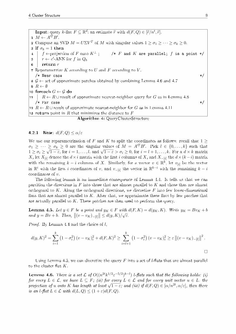
We now give a brief overview of the query algorithm, refer to Algorithm 4 for pseudocode.First, we check for the special case that F and K are parallel, i.e., that σ1 = · · · = σk = 1. Inthis case, we need to perform only a single c′-ANN query in Qb to obtain the desired result. IfF and K are not parallel, we distinguish two scenarios: if F is far from Q, we can approximateQ by its projection Qa onto K. Thus, we take the closest point xF in K to F , and we returnan approximate nearest neighbor for xF in Qa according to an appropriate metric derived fromLemma 4.4. Details can be found in Section 4.2.2. If F is close to Q, we use Lemma 4.4 todiscretize the relevant part of F into patches, such that each patch is parallel to K and suchthat the best nearest neighbor in Q for the patches provides an approximate nearest neighborfor F . Each patch can then be handled essentially by an appropriate nearest neighbor queryin K⊥. Details follow in Section 4.2.1. We say F and Q are close if d(F,Q) ≤ α/ε, and far ifd(F,Q) > α/ε. Recall that we chose ε = 1/100 log n.


Input: query k-�at F ⊆ Rd; an estimate r with d(F,Q) ∈ [r/nt, r].1 M ← A′TB′.2 Compute an SVD M = UΣV T of M with singular values 1 ≥ σ1 ≥ · · · ≥ σk ≥ 0.3 if σk = 1 then

4 f ←projection of F onto K⊥ ; /* F and K are parallel; f is a point */

5 r ← c′-ANN for f in Qb6 return r

7 Reparametrize K according to U and F according to V ./* Near case */

8 G ← set of approximate patches obtained by combining Lemma 4.6 and 4.79 R← ∅10 foreach G← G do11 R← R ∪ result of approximate nearest-neighbor query for G as in Lemma 4.8

/* Far case */

12 R← R ∪ result of approximate nearest-neighbor for G as in Lemma 4.1113 return point in R that minimizes the distance to F

Algorithm 4: QueryClusterStructure

4.2.1 Near: d(F,Q) ≤ α/ε

We use our reparametrization of F and K to split the coordinates as follows: recall that 1 ≥σ1 ≥ · · · ≥ σk ≥ 0 are the singular values of M = A′TB′. Pick l ∈ {0, . . . , k} such that1 ≥ σi ≥

√1− ε, for i = 1, . . . , l, and

√1− ε > σi ≥ 0, for i = l + 1, . . . , k. For a d× k matrix

X, let X[i] denote the d× i matrix with the �rst i columns of X, and X−[i] the d× (k− i) matrix

with the remaining k − i columns of X. Similarly, for a vector v ∈ Rk, let v[i] be the vector

in Ri with the �rst i coordinates of v, and v−[i] the vector in Rk−i with the remaining k − icoordinates of v.

The following lemma is an immediate consequence of Lemma 4.4. It tells us that we canpartition the directions in F into those that are almost parallel to K and those that are almostorthogonal to K. Along the orthogonal directions, we discretize F into few lower-dimensional�ats that are almost parallel to K. After that, we approximate these �ats by few patches thatare actually parallel to K. These patches are then used to perform the query.

Lemma 4.5. Let y ∈ F be a point and yK ∈ F with d(F,K) = d(yK ,K). Write yK = BvK + band y = Bv + b. Then,

∥∥(v − vK)−[l]

∥∥ ≤ d(y,K)/√ε.

Proof. By Lemma 4.4 and the choice of l,

d(y,K)2 =

k∑i=1

(1− σ2

i

)(v − vK)2

i + d(F,K)2 ≥k∑

i=l+1

(1− σ2

i

)(v − vK)2

i ≥ ε∥∥(v − vK)−[l]

∥∥2.

Using Lemma 4.5, we can discretize the query F into a set of l-�ats that are almost parallelto the cluster �at K.

Lemma 4.6. There is a set L of O((n2tk1/2ε−5/2)k−l) l-�ats such that the following holds: (i)for every L ∈ L, we have L ⊆ F ; (ii) for every L ∈ L and for every unit vector u ∈ L, theprojection of u onto K has length at least

√1− ε; and (iii) if d(F,Q) ∈ [α/n2t, α/ε], then there

is an l-�at L ∈ L with d(L,Q) ≤ (1 + ε)d(F,Q).


Proof. Let yK = BvK + b ∈ F be a point in F with d(F,K) = d(yK ,K). Furthermore, let

τ =αε

n2t√k

and oτ =

⌈n2t√k

ε5/2

⌉.

Using τ and στ , we de�ne a set I of index vectors with I = {−oττ, (−oτ + 1)τ, . . . , oττ}k−l and|I| = O(ok−lτ ) = O((n2tk1/2ε−5/2)k−l). For each i ∈ I, we de�ne the l-�at Li as

Li : w 7→ B[l]w +B−[l]

((vK)−[l] + i

)+ b.

Our desired set of approximate query l-�ats is now L = {Li | i ∈ I}.The set L meets properties (i) and (ii) by construction, so it remains to verify (iii). For

this, we take a point yQ ∈ F with d(F,Q) = d(yQ, Q). We write yQ = BvQ + b, and we de�nes = (vQ−vK)−[l]. We assumed that d(yQ,K) ≤ α/ε, so Lemma 4.5 gives ‖s‖ ≤ α/ε3/2. It followsthat by rounding each coordinate of s to the nearest multiple of τ , we obtain an index vectoriQ ∈ I with ‖iQ − s‖ ≤ τ

√k = εα/n2t. Hence, considering the point in LiQ with w = (vQ)[l],

we get

d(LiQ , Q) ≤ d(LiQ , yQ) + d(yQ, Q)

≤∥∥B[l](vQ)[l] +B−[l]

((vK)−[l] + iQ

)+ b−BvQ − b

∥∥+ d(F,Q)

=∥∥B−[l]

((vK)−[l] + iQ − (vQ)−[l]

)∥∥+ d(F,Q)

= ‖(vK − vQ)−[l] + iQ‖+ d(F,Q) (*)

= ‖iQ − s‖+ d(F,Q)

≤ εα/n2t + d(F,Q)

≤ (1 + ε)d(F,Q), (**)

where in (*) we used that the columns of B−[l] are orthonormal and in (**) we used the assump-tion d(F,Q) ≥ α/n2t.

From now on, we focus on an approximate query l-�at L. Our next goal is to approximateL by a set of patches such that each is parallel to K.

Lemma 4.7. There is a set G of O((n2tk1/2ε−2)l) patches such that the following holds: (i)every G ∈ G is an l-dimensional polytope, given by O(l) inequalities; (ii) for every G ∈ G, thea�ne hull of G is parallel to K; (iii) if d(L,Q) ∈ [α/n2t, 2α/ε], then there exists G ∈ G withd(G,Q) ≤ (1 + ε)d(L,Q); (iv) for all G ∈ G and for all q ∈ Q, we have d(G, q) ≥ (1− ε)d(L, q).

Proof. Let C = AATB1 be the d× l matrix whose columns b‖1, . . . , b

‖l constitute the projections

of the columns of B onto K. By Lemma 4.3, the vectors b‖i are orthogonal with ‖b

‖i ‖ = σi, for

i = 1, . . . , l, and the columns b⊥1 , . . . , b⊥l of the matrix B1−C also constitute an orthogonal set,

with ‖b⊥i ‖2 = 1− σ2i , for i = 1, . . . , l. Let zK be a point in L that minimizes the distance to K,

and write zK = B1wK + b1. Furthermore, let

τi =αε

n2t√l(1− σ2

i ), for i = 1, . . . , l, and oτ =

⌈2n2t√l

ε2

⌉.

We use the τi and oτ to de�ne a set I of index vectors as I =∏li=1{−oττi, (−oτ +1)τi, . . . , oττi}.

We have |I| = O(olτ ) = O((n2tk1/2ε−2)l). For each index vector i ∈ I, we de�ne the patch Gi as

Gi : w 7→ Cw +B1(wK + i) + b1, subject to w ∈l∏

i=1

[0, τi] .


Our desired set of approximate query patches is now G = {Gi | i ∈ I}. The set G ful�llsproperties (i) and (ii) by construction, so it remains to check (iii). Fix a point z ∈ L. SinceL ⊆ F , we can write z = B1w + b1 = Bv + b, where the vector w represents the coordinates ofz in L and the vector v represents the coordinates of z in F . By Lemma 4.4,

d(z,K)2 =k∑i=1

(1− σ2i )(v − vK)2

i + d(F,K)2,

where the vector vK represents the coordinates of a point in F that is closest to K. By de�nitionof L, the last k − l coordinates v−[l] in F are the same for all points z ∈ L, so we can concludethat the coordinates for a closest point to K in L are given by wK = (vK)[l] and that

d(z,K)2 =

l∑i=1

(1− σ2i )(w − wK)2

i + d(L,K)2. (3)

Now take a point zQ in L with d(zQ, Q) = d(L,Q) and write zQ = B1wQ+b1. Since we assumed

d(L,Q) ≤ 2α/ε, (3) implies that for i = 1, . . . , l, we have |(wQ−wK)i| ≤ 2α/(ε√

1 + σ2i

). Thus,

if for i = 1, . . . , l, we round (wQ − wK)i down to the next multiple of τi, we obtain an index

vector iQ ∈ I with (wQ − wK) − iQ ∈∏li=1 [0, τi]. We set sQ = (wQ − wK) − iQ. Considering

the point CsQ +B1(uK + iQ) + b1 in GiQ , we see that

d(GiQ , zQ)2 ≤ ‖CsQ +B1(wK + iQ) + b1 −B1wQ − b1‖2 = ‖CsQ −B1((wQ − wK)− iQ)‖2

= ‖(C −B1)sQ‖2 =l∑

i=1

(1− σ2i )(sQ)2

i ≤l∑

i=1

(1− σ2i )τ

2i = ε2α2/n4t,

using the properties of the matrix B1 − C stated above. It follows that

d(GiQ , Q) ≤ d(GiQ , zQ) + d(zQ, Q) ≤ εα/n2t + d(L,Q) ≤ (1 + ε)d(L,Q),

since we assumed d(L,Q) ≥ α/n2t. This proves (iii). Property (iv) is obtained similarly. LetGi ∈ G, q ∈ Q and let z be a point in Gi. Write z = Cw+B1(wK+i)+b1, where w ∈

∏ti=1 [0, σi].

Considering the point zx = B1(w + wK + i) + b1 in L, we see that

d(Gi, rx)2 ≤ ‖z − zx‖2 = ‖(C −B1)w‖ ≤ ε2α2/n4t.

Thus,d(Gi, q) ≥ d(zx, q)− d(Gi, zx) ≥ d(L, q)− εα/n2t ≥ (1− ε)d(L, q).

Finally, we have a patch G, and we are looking for an approximate nearest neighbor for Gin Q. The next lemma states how this can be done.

Lemma 4.8. Suppose that d(G,Q) ∈ [α/2n2t, 3α/ε]. We can �nd a point q ∈ Q with d(G, q) ≤(1− 1/2 log n)cd(G,Q) in total time Oc((k

2n2t/ε2)(m1−1/k+ρ/k + (d/k) logm)).

Proof. Let Ga be the projection of G onto K, and let g be the projection of G onto K⊥. SinceG and K are parallel, g is a point, and Ga is of the form Ga : w 7→ Cw + a2, with a2 ∈ Kand w ∈

∏ti=1[0, τi]. Let G+

a = {x ∈ K | d∞(x,Ga) ≤ 3α√k/ε}, where d∞(·, ·) denotes the

`∞-distance with respect to the coordinate system induced by A. We subdivide the set G+a \Ga,

into a collection C of axis-parallel cubes, each with diameter εα/2n2t. The cubes in C have sidelength εα/2n2t

√k, the total number of cubes is O((kn2t/ε2)k), and the boundaries of the cubes

lie on O(k2n2t/ε2) hyperplanes.


We now search the partition tree T to �nd the highest nodes (∆, Q) in T whose simplices∆ are completely contained in a single cube of C. This is done as follows: we begin at the rootof T , and we check for all children (∆, Q) and for all boundary hyperplanes h of C whether thesimplex ∆ crosses the boundary h. If a child (∆, Q) crosses no hyperplane, we label it with thecorresponding cube in C (or with Ga). Otherwise, we recurse on (∆, Q) with all the boundaryhyperplanes that it crosses.

In the end, we have obtained a set D of simplices such that each simplex in D is completelycontained in a cube of C. The total number of simplices in D is s = O((k2n2t/ε2)m1−1/k),by Theorem 3.1. For each simplex in D, we query the corresponding c′-ANN structure. LetR ⊆ Qb be the set of the query results. For each point qb ∈ R, we take the corresponding pointq ∈ Q, and we compute the distance d(q,G). We return a point q that minimizes d(q,G). Thequery time is dominated by the time for the ANN queries. For each ∆ ∈ D, let m∆ be thenumber of points in the corresponding ANN structure. By assumption, an ANN-query takestime Oc(m

ρ∆ + d logm∆), so the total query time is proportional to

∑∆∈D

mρ∆ + d logm∆ ≤ s

(∑∆∈D

m∆/s

)ρ+ sd log

(∑∆∈D

m∆/s

)≤ Oc

((k2n2t/ε2)(m1−1/k+ρ/k + (d/k) logm)

),

using the fact that m 7→ mρ + d logm is concave and that∑

∆∈Dm∆ ≤ m.It remains to prove that approximation bound. Take a point q∗ in Q with d(q∗, Q) = d(Q,G).

Since we assumed that d(Q,G) ≤ 3α/ε, the projection q∗a of q∗ onto K lies in G+

a . Let ∆∗ be thesimplex in D with q∗a ∈ ∆∗. Suppose that the ANN-query for ∆∗ returns a point q ∈ Q. Thus,in K⊥, we have d(qb, g) ≤ c′d(Qb∆∗ , g) ≤ c′d(q∗b , g), where qb and q

∗b are the projections of q and

q∗ onto K⊥ and Qb∆∗ is the point set stored in the ANN-structure of ∆∗. By the de�nitionof C, in K, we have d(qa, Ga) ≤ d(q∗a, Ga) + εα/2n2t ≤ d(q∗a, Ga) + εd(q∗, G), where qa is theprojection of q onto K. By Pythagoras,

d(q, G)2 = d(qb, g)2 + d(qa, Ga)2

≤ c′2d(q∗b , g)2 + (d(q∗a, Ga) + εd(q∗, G))2

≤ c′2d(q∗b , g)2 + d(q∗a, Ga)2 + (2ε+ ε2)d(q∗, G)2

≤ (c′2 + 3ε)(q∗, G)2

≤((1− 1/ log n)2c2 + 3/100 log n

)(q∗, G)2

≤ (1− 1/2 log n)2c2(q∗, G)2,

recalling that c′ = (1 − 1/ log n)c and ε = 1/100 log n. Since d(q, G) ≤ d(q, G), the resultfollows.

Of all the candidate points obtained through querying patches, we return the one closest to F .The following lemma summarizes the properties of the query algorithm.

Lemma 4.9. Suppose that d(F,Q) ∈ [α/n2t, α/ε]. Then the query procedure returns a pointq ∈ Q with d(F, q) ≤ cd(F,Q) in total time Oc((k

2n2tε−5/2)k+1(m1−1/k+ρ/k + (d/k) logm)).

Proof. By Lemmas 4.6 and 4.7, there exists a patch G with d(G,Q) ≤ (1 + ε)2d(F,Q). For thispatch, the algorithm from Lemma 4.8 returns a point q with d(q, G) ≤ (1 + 1/2 log n)cd(G,Q).Thus, using Lemma 4.7(iv), we have

(1− ε)d(q, L) ≤ d(q, G) ≤ (1− 1/2 log n)c(1 + ε)2d(F,Q)


and by our choice of ε = 1/100 log n, we get

(1− 1/2 log n)(1 + ε)2/(1− ε) ≤ (1− 1/2 log n)(1 + 3ε)(1 + 2ε)

≤ (1− 1/2 log n)(1 + 6/100 log n) ≤ 1.

4.2.2 Far: d(F,Q) ≥ α/ε

If d(F,Q) ≥ α/ε, we can approximate Q by its projection Qa onto K without losing toomuch. Thus, we can perform the whole algorithm in K. This is done by a procedure simi-lar to Lemma 4.8.

Lemma 4.10. Suppose we are given an estimate r with d(F,Qa) ∈ [r/2nt, 2r]. Then, we can�nd a point q ∈ Qa with d(F, q) ≤ (1 + ε)d(F,Qa) in time O((k3/2nt/ε)m1−1/k).

Proof. Let xF be a point in K with d(F,K) = d(F, xF ). Write xF = AuF + a. De�ne

C =

k∏i=1

((uF )i +

[0, 2r/

√1− σ2

i

])If we take a point x ∈ K with d(x, F ) ∈ [r/2nt, 2r] and write x = Au+a, then Lemma 4.4 gives

d(F, x)2 =

k∑i=1

(1− σ2i )(u− uF )2

i + d(F,K)2,

so u ∈ C. We subdivide C into copies of the hyperrectangle∏ki=1[0, εr/2nt

√k(1− σ2

i )]. Let

C be the resulting set of hyperrectangles. The boundaries of the hyperrectangles in C lie onO(k3/2nt/ε) hyperplanes. We now search the partition tree T in order to �nd the highest nodes(∆, Q) in T whose simplices ∆ are completely contained in a single hyperrectangle of C. This isdone in the same way as in Lemma 4.8.

This gives a set D of simplices such that each simplex in D is completely contained in ahyperrectangle of C. The total number of simplices in D is O((k3/2nt/ε)m1−1/k), by Theorem 3.1.For each simplex ∆ ∈ D, we pick an arbitrary point q ∈ Qa that lies in ∆, and we computed(F, q). We return the point q ∈ Qa that minimizes the distance to F . The total query time isO((k3/2nt/ε)m1−1/k).

Now let q∗ be a point in Qa with d(F,Qa) = d(F, q∗), and let ∆∗ be the simplex D thatcontains q∗. Furthermore, let q ∈ Qa be the point that the algorithm examines in ∆∗. Writeq∗ = Au∗+ a and q = Au+ a. Since q∗ and q lie in the same hyperrectangle and by Lemma 4.4,

d(F, q)2 =

k∑i=1

(1− σ2i )(u− uF )2

i + d(F,K)2 ≤

k∑i=1

(1− σ2i )(u

∗ − uF )2i + ε2r2/4n2t + d(F,K)2 ≤ (1 + ε)2d(F, q∗)2.

Since d(F, q) ≤ d(F, q), the result follows.

Lemma 4.11. Suppose we are given an estimate r with d(F,Q) ∈ [r/nt, r]. Suppose further thatd(F,Q) ≥ α/ε. Then we can �nd a q ∈ Q with d(F, q) ≤ cd(F,Q) in time O((k3/2n2t/ε)m1−1/k).

5 Approximate k-�at Range Reporting in Low Dimensions 14

Proof. For any point q ∈ Q, let qa ∈ Q be its projection onto K. Then, d(qa, q) ≤ α ≤ εd(F,Q).Thus, d(F,Qa) ∈ [(1 − ε)d(F,Q), (1 + ε)d(F,Q)], and we can apply Lemma 4.10. Let qa ∈ Qabe the result of this query, and let q be the corresponding point in Q. We have

d(F, q) ≤ d(q, qa) + d(F, qa) ≤ εd(F,Q) + (1 + ε)d(F,Qa)

≤ εd(F,Q) + (1 + ε)2d(F,Q) ≤ (1 + 4ε)d(F,Q) ≤ cd(F,Q),

by our choice of ε.

By combining Lemmas 4.1, 4.9, and 4.11, we obtain Theorem 2.1.

5 Approximate k-�at Range Reporting in Low Dimensions

In this section, we present a data structure for low dimensional k-�at approximate near neighborreporting. In Section 6, we will use it as a foundation for our projection structures. The detailsof the structure are summarized in Theorem 5.1. Throughout this section, we will think of d asa constant, and we will suppress factors depending on d in the O-notation.

Theorem 5.1. Let P ⊂ Rd be an n-point set. We can preprocess P into an O(n logd−k−1 n) spacedata structure for approximate k-�at near neighbor queries: given a k-�at F and a parameterα, �nd a set R ⊆ P that contains all p ∈ P with d(p, F ) ≤ α and no p ∈ P with d(p, F ) >((4k + 3)(d− k − 1) +

√k + 1)α. The query time is O(nk/(k+1) logd−k−1 n+ |R|).

5.1 Preprocessing

Let E ⊂ Rd be the (k + 1)-dimensional subspace of Rd spanned by the �rst k + 1 coordinates,and let Q be the projection of P onto E.1 We build a (k + 1)-dimensional partition tree T forQ, as in Theorem 3.1. If d > k + 1, we also build a slab structure for each node of T . Let v besuch a node, and let Ξ be the simplicial partition for the children of v. Let w > 0. A w-slab Sis a closed region in E that is bounded by two parallel hyperplanes of distance w. The medianhyperplane h of S is the hyperplane inside S that is parallel to the two boundary hyperplanesand has distance w/2 from both. A w-slab S is full if there are at least r2/3 simplices ∆ in Ξwith ∆ ⊂ S.

Input: point set P ⊂ Rd1 if |P | = O(1) then2 Store P in a list and return.3 Q← projection of P onto the subspace E spanned by the �rst k + 1 coordinates.4 T ← (k + 1)-dimensional partition tree for Q as in Theorem 3.1.5 if d > k + 1 then

6 foreach node v ∈ T do

7 Ξ1 ← simplicial partition for the children of v

8 for j ← 1 to br1/3c do9 Dj ← CreateSlabStructure(Ξj)10 Ξj+1 ← Ξj without all simplices inside the slab for Dj

Algorithm 5: CreateSearchStructure

The slab structure for v is constructed in several iterations. In iteration j, we have a currentsubset Ξj ⊆ Ξ of pairs in the simplicial partition. For each (k + 1)-set v0, . . . , vk of verticesof simplices in Ξj , we determine the smallest width of a full slab whose median hyperplane

is spanned by v0, . . . , vk. Let Sj be the smallest among those slabs, and let hj be its median

1 We assume general position: any two distinct points in P have distinct projections in Q.


Input: Ξj = (Q1,∆1), . . . , (Qr′ ,∆r′)1 Vj ← vertices of the simplices in Ξj2 For each (k + 1)-subset V ⊂ Vj , �nd the smallest wV > 0 such that the wV -slab withmedian hyperplane aff(V ) is full.

3 Let wj be the smallest wV ; let Sj be the corresponding full wj-slab and hj = aff(V ) itsmedian hyperplane.

4 Find the set Dj of r2/3 simplices in Sj ; let Qj ←⋃

∆i∈DjQi and let Pj be the

d-dimensional point set corresponding to Qj .5 hj ← the hyperplane orthogonal to E through hj6 P ′ ← projection of Pj onto hj /* P ′ is (d− 1)-dimensional */

7 CreateSearchStructure(P ′)Algorithm 6: CreateSlabStructure

hyperplane. Let Dj be the r2/3 simplices that lie completely in Sj . We remove Dj and thecorresponding point set Qj =

⋃∆i∈Dj

Qi from Ξj to obtain Ξj+1. Let Pj ⊆ P be the d-dimensional point set corresponding to Qj . We project Pj onto the d-dimensional hyperplane

hj that is orthogonal to E and goes through hj . We recursively build a search structure for the(d − 1)-dimensional projected point set. The jth slab structure Dj at v consists of this searchstructure, the hyperplane hj , and the width wj . This process is repeated until less than r2/3

simplices remain; see Algorithms 5 and 6 for details.Denote by S(n, d) the space for a d-dimensional search structure with n points. The partition

tree T has O(n) nodes, so the overhead for storing the slabs and partitions is linear. Thus,

S(n, d) = O(n) +∑D

S(nD, d− 1),

where the sum is over all slab structures D and where nD is the number of points in the slabstructure D. Since every point appears in O(log n) slab structures, and since the recursion stopsfor d = k + 1, we get

Lemma 5.2. The search structure for n points in d dimensions needs space O(n logd−k−1 n).

5.2 Processing a Query

For a query, we are given a distance threshold α > 0 and a k-�at F . For the recursion, we willneed to query the search structure with a k-dimensional polytope. We obtain the initial querypolytope by intersecting the �at F with the bounding box of P extended by α in each direction.With slight abuse of notation, we still call this polytope F .

A query for F and α is processed by using the slab structures for small enough slabs and byrecursing in the partition tree for the remaining points. Details follow.

Suppose we are at some node v of the partition tree, and let j∗ be the largest integer withwj∗ ≤ (4k + 2)α. For j = 1, . . . , j∗, we recursively query each slab structure Dj as follows: let

F ⊆ F be the polytope containing the points in F with distance at most α + wj/2 from hj ,

and let Fh be the projection of F onto hj . We query the search structure in Dj with Fh andα. Next, we project F onto the subspace E spanned by the �rst k + 1 coordinates. Let D bethe simplices in Ξj∗+1 with distance at most α from the projection. For each simplex in D, werecursively query the corresponding child in the partition tree. Upon reaching the bottom of therecursion (i.e., |P | = O(1)), we collect all points within distance α from F in the set R.

If d = k+1, we approximate the region of interest by the polytope F� = {x ∈ Rd | d1(x, F ) ≤α}, where d1(·, ·) denotes the `1-metric in Rd. Then, we query the partition tree T to �nd allpoints of P that lie inside F�. We prove in Lemma 5.4 that F� is a polytope with O(dO(k2))


Input : polytope F , distance threshold α > 0Output: point set R ⊆ P

1 R← ∅2 if |P | = O(1) then3 R← {p ∈ P | d(p, F ) ≤ α}4 else if d = k + 1 then

5 Compute polytope F� as described.6 R← R ∪ all points of P inside F�7 else

8 j∗ ← the largest integer with wj∗ ≤ (4k + 2)α9 for j ← 1 to j∗ do

10 Fh ← projection of F onto hj as described11 R← R ∪Dj .query(Fh, α)

12 F ← projection of F onto the subspace E spanned by the �rst k + 1 coordinates13 D ← simplices in Ξj∗+1

14 D′ ← {∆ ∈ D | d(∆, F ) ≤ α}15 foreach ∆ ∈ D′ do16 R← R ∪ result of recursive query to partition tree node for ∆.

17 return RAlgorithm 7: Find a superset R of all points in P with distance less than α from a querypolytope F .

facets; see Algorithm 7 for details. The following two lemmas analyze the correctness and querytime of the algorithm.

Lemma 5.3. The set R contains all p ∈ P with d(p, F ) ≤ α and no p ∈ P with d(p, F ) > κα,where κ = (4k + 3)(d− k − 1) +

√k + 1.

Proof. The proof is by induction on the size n of P and on the dimension d. If n = O(1), wereturn all points with distance at most α to F . If d = k + 1, we report the points inside thepolytope F� (lines 4�6) using T . Since ‖x‖2 ≤ ‖x‖1 ≤

√k + 1‖x‖2 holds for all x ∈ Rk+1, the

polytope F� contains all points with distance at most α from F and no point with distance morethan α

√k + 1 from F . Thus, correctness also follows in this case.

hj

F

q

qqF

qF

α

wj hj

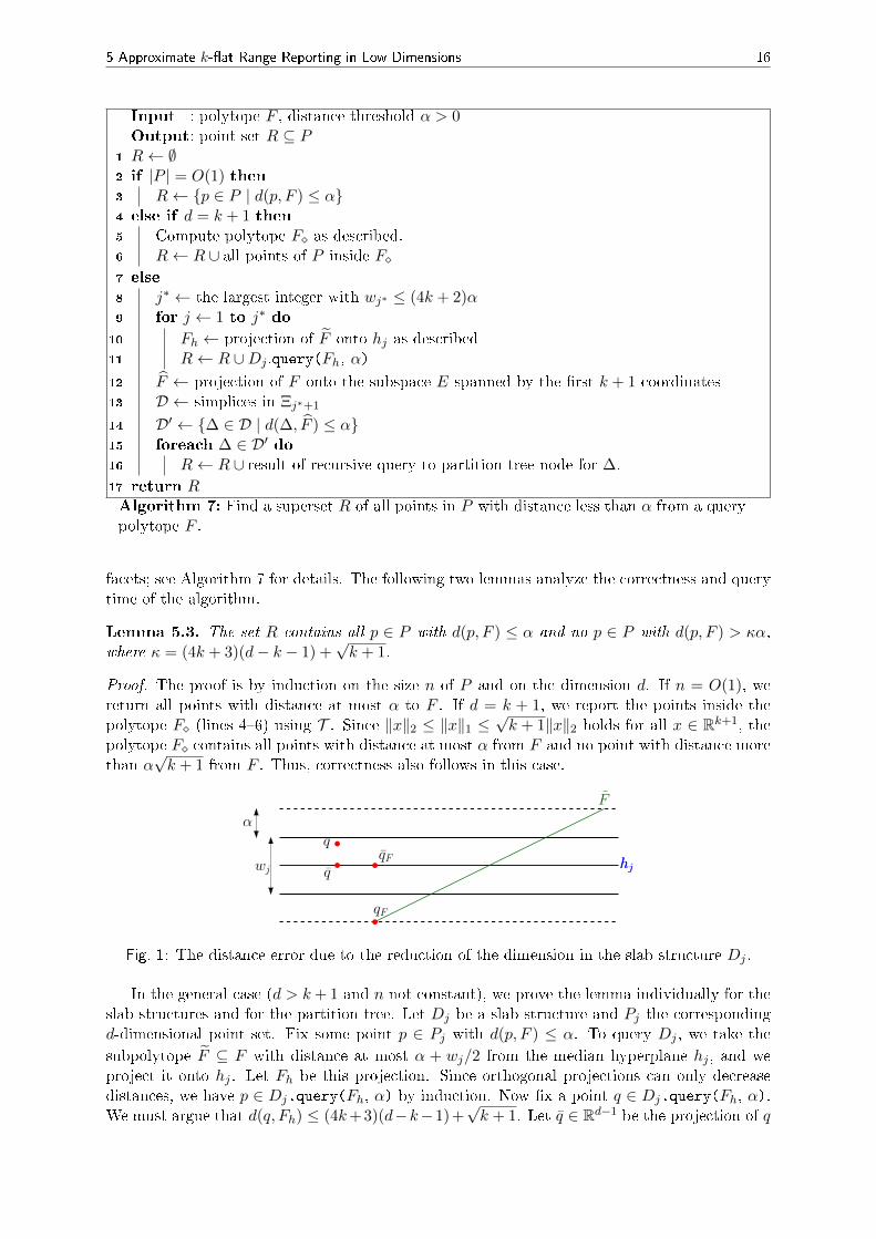
Fig. 1: The distance error due to the reduction of the dimension in the slab structure Dj .

In the general case (d > k+ 1 and n not constant), we prove the lemma individually for theslab structures and for the partition tree. Let Dj be a slab structure and Pj the correspondingd-dimensional point set. Fix some point p ∈ Pj with d(p, F ) ≤ α. To query Dj , we take the

subpolytope F ⊆ F with distance at most α + wj/2 from the median hyperplane hj , and weproject it onto hj . Let Fh be this projection. Since orthogonal projections can only decreasedistances, we have p ∈ Dj.query(Fh, α) by induction. Now �x a point q ∈ Dj.query(Fh, α).We must argue that d(q, Fh) ≤ (4k+3)(d−k−1)+

√k + 1. Let q ∈ Rd−1 be the projection of q


onto hj and qF ∈ Fh the closest point to q in Fh. Let qF ∈ F be the corresponding d-dimensionalpoint (see Fig. 1). By triangle inequality and the induction hypothesis,

d(q, F ) = d(q, F ) ≤ d(q, q) + d(q, qF ) + d(qF , qF )

≤ wj/2 + ((4k + 3)(d− k − 2) +√k + 1)α+ (α+ wj/2).

By construction, we have wj ≤ (4k + 2)α, so d(q, F ) ≤ ((4k + 3)(d − k − 1) +√k + 1)α, as

claimed.Consider now a child in the partition tree queried in line 16, and let Pj be the corresponding

d-dimensional point set. Since |Pj | < |P |, the claim follows by induction.

Lemma 5.4. The query time is O(nk/(k+1) logd−k−1 n+ |R|).

Proof. Let Q(n, d) be the total query time.First, let d > k + 1. We bound the time to query the partition tree T . Let F be the

projection of F onto E. Furthermore, let V be the set of nodes in T that are visited duringa query, and let D be the corresponding simplices. By construction, all simplices in D havedistance at most α from F . Consider the 2α-slab S whose median hyperplane contains F . Wepartition V into two sets: the nodes VB whose simplices intersect ∂S, and the nodes VC whosesimplices lie completely in S. First, since the simplex for each node in T is contained in thesimplex for its parent node, we observe that VB constitutes a connected subtree of T , startingat the root. The nodes of VC form several connected subtrees, each hanging o� a node in VB.Furthermore, by construction, each node from V has at most r1/3 children from VB. Let V` bethe set of nodes in V with level `, for ` = 0, . . . , logr n, and let m` = |V`|. By Theorem 3.1, wehave |V` ∩ VB| ≤ O(r`k/(k+1) + r(k−1)/km`−1 + r` log r log n). Since |V` ∩ VC | ≤ r1/3m`−1, we get

m` = |V`| = O(r`k/(k+1) + (r(k−1)/k + r1/3)m`−1 + r` log r log n

).

For any δ > max(0, 1/3− (k− 1)/k), if we choose r large enough depending on δ, this solves tom` = O(r`k/(k+1) + r`((k−1)/k+δ) log n). Thus, we get

Q(n, d) =

logr n∑`=0

O(r`k/(k+1) + r`((k−1)/k+δ) log n)(O(r) +Q(n/r`, d− 1)). (4)

For d = k + 1, we use T directly. Thus, by Theorem 3.1, the query time Q(n, k + 1) isO(fk+1n

1−1/k + |RF |), where fk+1 is the number of facets of F♦ and RF is the answer set. Weclaim that fk+1 is bounded by ((2k + 2)(5d0 − 2k)k/2)(k+1)/2. Recall that F� is the Minkowskisum of F and the `1-ball with radius α as in Algorithm 7 line 5. Initially F is the intersectionof the query k-�at with the extended bounding box of P . This intersection can be described byat most d0 − k + 2d0 = 3d0 − k oriented half-spaces, where d0 denotes the initial dimension. Ineach recursive step, we intersect F with the 2 bounding hyperplanes of a slab. Therefore, thedescriptive complexity of F in the base case is at most 5d0 − 2k. By duality and the UpperBound theorem [17], the V-description of F consists of at most (5d0 − 2k)k/2 vertices. Usingthat the Minkowski sum of two polytopes with v1 and v2 vertices has at most v1v2 vertices, wededuce that F� has at most (2k + 2)(5d0 − 2k)k/2 vertices. Applying the upper bound theoremagain, it follows that fk+1 = ((2k + 2)(5d0 − 2k)k/2)(k+1)/2, as claimed.

Thus, plugging the base case into (4), we get that the overall query time Q(n, d) is boundedby O(nk/(k+1) logd−k−1 +|R|).

Theorem 5.1 follows immediately from Lemmas 5.2, 5.3, and 5.4.

6 Projection Structures 18

5.3 Approximate k-Flat Nearest Neighbor Queries

We now show how to extend our data structure from Section 5.1 for approximate k-�at nearestneighbor queries with multiplicative error (4k + 3)(d − k − 1) +

√k + 1. That is, given an

n-point set P ⊂ Rd, we want to �nd for any given query �at F ⊂ Rd a point p ∈ P withd(p, F ) ≤ ((4k + 3)(d − k − 1) +

√k + 1)d(P, F ). We reduce this problem to a near neighbor

query by choosing an appropriate threshold α that ensures |R| = O(√n), using random sampling.

For preprocessing we build the data structure D from Theorem 5.1 for P .Let a query �at F be given. The F -rank of a point p ∈ P is the number of points in P that

are closer to F than p. Let X ⊆ P be a random sample obtained by taking each point in Pindependently with probability 1/

√n. The expected size of X is

√n, and if x ∈ X is the closest

point to F in X, then the expected F -rank of x is√n. Set α = d(x, F )/((4k + 3)(d− k − 1) +√

k + 1). We query D with F and α to obtain a set R. If d(P, F ) ≤ α, then R contains thenearest neighbor. Otherwise, x is a ((4k+3)(d−k−1)+

√k + 1)-approximate nearest neighbor

for F . Thus, it su�ces to return the nearest neighbor in R∪{x}. Since with high probability allpoints in R have F -rank at most O(

√n log n), we have |R| = O(

√n log n), and the query time

is O(nk/(k+1) logd−k−1 n). This establishes the following corollary of Theorem 5.1.

Corollary 5.5. Let P ⊂ Rd be an n-point set. We can preprocess P into an O(n logd−k−1 n)space data structure for approximate k-�at nearest neighbor queries: given a �at F , �nd a pointp ∈ P with d(p, F ) ≤ ((4k + 3)(d − k − 1) +

√k + 1)d(P, F ). The expected query time is

O(nk/(k+1) logd−k−1 n).

6 Projection Structures

We now describe how to answer queries of type Q1 and Q3 e�ciently. Our approach is toproject the points into random subspace of constant dimension and to solve the problem thereusing our data structures from Theorem 5.1 and Corollary 5.5. For this, we need a Johnson-Lindenstrauss-type lemma that bounds the distortion, see Section 6.1.

Let 0 < t ≤ 2/(2 + 40k) be a parameter and let P ⊂ Rd be a high dimensional n-pointset. Set d′ = 2/t + 2 and let M ∈ Rd′×d be a random projection from Rd to Rd′ , scaled by√d/4d′. We obtain P ⊂ Rd′ by projecting P using M . We build for P the data structure D1

from Corollary 5.5 to answer Q1 queries and D2 from Theorem 5.1 to answer Q3 queries. Thisneeds O(n logO(d′) n) = O(n logO(1/t) n) space. For each p ∈ P we write p for the d′-dimensionalpoint Mp and F for the projected �at MF .

6.1 Dimension Reduction

We use the following variant of the Johnson-Lindenstrauss-Lemma, as proved by Dasgupta andGupta [8, Lemma 2.2].

Lemma 6.1 (JL-Lemma). Let d′ < d, and let M ∈ Rd′×d be the projection matrix onto arandom d′-dimensional subspace, scaled by a factor of

√d/d′. Then, for every vector x ∈ Rd of

unit length and every β > 1, we have

1. Pr[‖Mx‖2 ≥ β

]≤ exp

(12d′(1− β + lnβ)

), and

2. Pr[‖Mx‖2 ≤ 1/β

]≤ exp

(12d′(1− 1/β − lnβ)

)≤ exp

(12d′(1− lnβ)

).

Lemma 6.2. Let p ∈ Rd be a point and let F ⊂ Rd be a k-�at. For d′ ∈ {40k, . . . , d − 1}, letM ∈ Rd′×d be the projection matrix into a random d′-dimensional subspace, scaled by

√d/4d′.

Let p = Mp and F = MF be the projections of p and of F , respectively. Then, for any β ≥ 40k,(i) Pr[d(p, F ) ≤ d(p, F )] ≥ 1− e−d′/2; and (ii) Pr[d(p, F ) ≥ d(p, F )/β] ≥ 1− β−d′/2.


Proof. Let N = 2M , and set q = Np and K = NF . De�ning ∆p = d(p, F ) and ∆q = d(q,K),we must bound the probabilities Pr[∆q ≤ 2∆p] for (i) and Pr[∆q ≥ 2∆p/β] for (ii).

We begin with (i). Let p‖ be the orthogonal projection of p onto F , and let p⊥ = p−p‖. Letq⊥ = Np⊥. Then, ∆p = ‖p⊥‖ and ∆q ≤ ‖q⊥‖. By Lemma 6.1(1),

Pr[‖q⊥‖ ≥ 2∆p

]= Pr

[‖Np⊥‖/‖p⊥‖ ≥ 2

]= Pr

[‖N(p⊥/‖p⊥‖)‖2 ≥ 4

]≤ exp

(12d′(1− 4 + ln 4)

)≤ exp(−d′/2).

Thus, Pr[∆q ≤ 2∆p] ≥ Pr[‖q⊥‖ ≤ 2∆p] ≥ 1− exp(−d′/2), as desired.

For (ii), choose k orthonormal vectors e1, . . . , ek such that F ={p‖ +

∑ki=1 λiei | λi ∈ R

}.

Set ui = ei‖p⊥‖/β2, and consider the lattice L ={p‖ +

∑ki=1 µiui | µi ∈ Z

}⊂ F . Let L = NL

be the projected lattice. We next argue that with high probability (i) all points in L havedistance at least 3‖p⊥‖/β from q; and (ii) for i = 1, . . . , k, we have ‖Nui‖ < ‖p⊥‖/β

√k.

To show (i), we partition L into layers: for j ∈ {0, 1, . . . , }, let

Lj =

{p‖ +

k∑i=1

µiui | µi ∈ {−j, . . . , j},maxi|µi| = j

}⊂ L.

Now for any j ∈ N and r = p‖ +∑k

i=1 µiui ∈ Lj , Pythagoras gives

‖p− r‖ =

√√√√‖p⊥‖2 +

∥∥∥∥∥k∑i=1

µiui

∥∥∥∥∥2

= ‖p⊥‖

√√√√1 +k∑i=1

|µi|2/β4 ≥ ‖p⊥‖√

1 + j2/β4.

Thus, using Lemma 6.1(2),

Pr[‖N(p− r)‖ ≤ 3‖p⊥‖/β

]= Pr

[‖N(p− r)‖/‖p− r‖ ≤ 3‖p⊥‖/β‖p− r‖

]≤ Pr

[‖N(p− r)/‖p− r‖‖2 ≤ 9/β2(1 + j2/β4)

]≤ exp(1

2d′(1 + ln(9/β2(1 + j2/β4))))

≤ (5/β)d′(1 + j2/β4)−d

′/2,

as√

9e ≤ 5. Now we use a union bound to obtain

Pr[∃r ∈ L : ‖N(p− r)‖ ≤ 3‖p⊥‖/β

]=∞∑j=0

Pr[∃r ∈ Lj : ‖N(p− r)‖ ≤ 3‖p⊥‖/β

].

Grouping the summands into groups of β2 consecutive terms, this is

=∞∑l=0

lβ2+β2−1∑j=lβ2

Pr[∃r ∈ Lj : ‖N(p− r)‖ ≤ 3‖p⊥‖/β

]≤ (5/β)d

′∞∑l=0

|L≤(l+1)β2 |(1 + (lβ2)2/β4)−d′/2,

where L≤a =⋃ai=0 Li. Using the rough bound |L≤a| ≤ (3a)k, this is

≤ (5/β)d′∞∑l=0

(3(l + 1)β2)k(1 + l2)−d′/2

= 5d′3kβ2k−d′

∞∑l=0

(l + 1)k(1 + l2)−d′/2.


For d′ ≥ 4k, we have (l + 1)k(1 + l2)−d′/2 ≤ (l + 1)k(1 + l2)−2k ≤ 1/(1 + l2), so we can bound

the sum by∑∞

l=1 1/(1 + l2) ≤ π2/6. Thus, we have derived

Pr[∃r ∈ L : ‖N(p− r)‖ ≤ 3‖p⊥‖/β

]≤ 5d

′3kβ2k−d′(π2/6) ≤ 5d

′+kβ2k−d′ , (5)

since π2/6 ≤ 5/3.

To show (ii), we use a union bound with Lemma 6.1(1). Recalling ‖u1‖ = ‖p⊥‖/β2,

Pr[∃i = 1, . . . , k : ‖Nui‖ > ‖p⊥‖/

√kβ]≤ kPr

[‖Nu1‖ > ‖p⊥‖/

√kβ]

= kPr[‖N(u1/‖u1‖)‖2 > β2/k]

≤ k exp(

12d′(1− β2/k + ln(β2/k))

)≤ k exp

(−β2d′/4k

), (6)

since c2/k ≥ 2(1 + ln(β2/k)) for β2/k ≥ 6. By (5) and (6), and recalling β, d′ ≥ 40k, theprobability that events (i) and (ii) do not both happen is at most

5d′+kβ2k−d′ + ke−β

2d′/4k ≤ 5(1+1/40)d′β(1/20−1)d′ + (β/40)e−10cd′

≤

(541/40

409/20

)d′β−d

′/2 +1

10β−d

′/2 ≤ β−d′/2.

Suppose (i) and (ii) happen. Fix a point w ∈ K, and let r ∈ L be the point in the projectedlattice that is closest to w. By (i), d(q, r) > 3‖p⊥‖/β. By (ii) and the choice of r, the k-dimensional cube with center r and side length ‖p⊥‖/β

√k contains w. This cube has diameter

‖p⊥‖/β. By triangle inequality, d(q, w) > d(q, r)− d(r, w) ≥ (3/β − 1/β)‖p⊥‖ = 2‖p⊥‖/β.

6.2 Queries of Type Q1

Let a query �at F be given. To answer Q1 queries, we compute F and query D1 with F toobtain a ((4k+ 3)(d′ − k− 1) +

√k + 1)-nearest neighbor p. We return the original point p. To

obtain Theorem 2.2, we argue that if p is a ((4k + 3)(d− k − 1) +√k + 1)-nearest neighbor for

F , then p is a nt-nearest neighbor for F with high probability.Let p∗ ∈ P be a point with d(p∗, F ) = d(P, F ). Set δp∗ = d(p∗, F ) and δp∗ = d(p∗, F ).

Denote by A1 the event that δp∗ ≤ δp∗ . By Lemma 6.2, Pr[A1] ≥ 1− e−d′/2 = 1− e−1/t−1. LetA2 be the event that for all points p ∈ P with δp = d(p, F ) > ntδp∗ we have δp = d(p, F ) >((4k+3)(d′−k−1)+

√k + 1)δp∗ . For a �xed p ∈ P , by setting β = nt/((4k+3)(d′−k−1)+

√k + 1)

in Lemma 6.2, this probability is seen to be at least 1 − n−1−t/2, for n large enough. By theunion bound, we get Pr[A2] ≥ 1− n−t/2, so the event A1 ∩A2 occurs with constant probability.Then, p is a nt-approximate nearest neighbor for F , as desired.

6.3 Queries of Type Q3

To answer a query of type Q3, we compute the projection F and query D2 with parameter α.We obtain a set R ⊂ P in time O(nk/(k+1) logO(1/t) n + |R|). Let R ⊂ P be the correspondingd-dimensional set. We return a point p ∈ R that minimizes d(p, F ). If δp∗ ≤ α, the event A1

from above implies that p∗ ∈ R, and we correctly return p∗.To bound the size of |R|, and thus the running time, we use that P is αnt/(2k + 1)-cluster-

free. Let A3 be the event that for all p ∈ P with d(p, F ) > αnt/(2k+1), we have d(p, F ) > ((4k+

7 Conclusion 21

3)(d′−k−1)+√k + 1)α. By the de�nition of cluster-freeness and the guarantee of Theorem 5.1,

we have |R| = m in the case of A3. Using β = nt/((2k + 1)((4k + 3)(d − k − 1) +√k + 1))

in Lemma 6.2 and doing a similar calculation as above yields again Pr[A3] ≥ 1 − n−t/2. Thus,we can answer queries of type Q3 successfully in time O(nk/(k+1) logO(1/t) n+m) with constantprobability, as claimed in Theorem 2.3.

7 Conclusion

We have described the �rst provably e�cient data structure for general k-ANN. Our maintechnical contribution consists of two new data structures: the cluster data structure for high-dimensional k-ANN queries, and the projection data structure for k-ANN queries in constantdimension. We have only presented the latter structure for a constant approximation factor(4k + 3)(d − k − 1) +

√k + 1, but we believe that it is possible to extend it to any �xed

approximation factor c > 1. For this, one would need to subdivide the slab structures by asu�ciently �ne sequence of parallel hyperplanes.

Naturally, the most pressing open question is to improve the query time of our data structure.Also, a further generalization to more general query or data objects would be of interest.

Acknowledgments

This work was initiated while WM, PS, and YS were visiting the Courant Institute of Math-ematical Sciences. We would like to thank our host Esther Ezra for her hospitality and manyenlightening discussions.

References

[1] A. Andoni. Nearest Neighbor Search: the Old, the New, and the Impossible. PhD thesis,Massachusetts Institute of Technology, 2009.

[2] A. Andoni, P. Indyk, R. Krauthgamer, and H. L. Nguyen. Approximate line nearest neigh-bor in high dimensions. In Proc. 20th Annu. ACM-SIAM Sympos. Discrete Algorithms(SODA), pages 293�301, 2009.

[3] A. Andoni, P. Indyk, H. L. Nguyen, and I. Razenshteyn. Beyond locality-sensitive hashing.In Proc. 24th Annu. ACM-SIAM Sympos. Discrete Algorithms (SODA), pages 1018�1028,2014.

[4] R. Basri, T. Hassner, and L. Zelnik-Manor. Approximate nearest subspace search withapplications to pattern recognition. In Proc. Conference on Computer Vision and PatternRecognition (CVPR), pages 1�8, 2007.

[5] T. M. Chan. Optimal partition trees. Discrete Comput. Geom., 47(4):661�690, 2012.

[6] B. Chazelle. The discrepancy method. Randomness and complexity. Cambridge UniversityPress, 2000.

[7] K. L. Clarkson. A randomized algorithm for closest-point queries. SIAM J. Comput.,17(4):830�847, 1988.

[8] S. Dasgupta and A. Gupta. An elementary proof of a theorem of Johnson and Lindenstrauss.Random Structures Algorithms, 22(1):60�65, 2003.

[9] R. A. Horn and C. R. Johnson. Matrix analysis. Cambridge University Press, secondedition, 2013.

7 Conclusion 22

[10] P. Indyk. Nearest neighbors in high-dimensional spaces. In J. E. Goodman and J. O'Rourke,editors, Handbook of Discrete and Computational Geometry, chapter 39. CRC Press, 2ndedition, 2004.

[11] P. Indyk and R. Motwani. Approximate nearest neighbors: towards removing the curseof dimensionality. In Proc. 30th Annu. ACM Sympos. Theory Comput. (STOC), pages604�613, 1998.

[12] E. Kushilevitz, R. Ostrovsky, and Y. Rabani. E�cient search for approximate nearestneighbor in high dimensional spaces. In Proc. 30th Annu. ACM Sympos. Theory Comput.(STOC), pages 614�623, 1998.

[13] Q. Lv, W. Josephson, Z. Wang, M. Charikar, and K. Li. Multi-probe LSH: E�cient indexingfor high-dimensional similarity search. In Proc. 33rd International Conference on Very LargeData Bases (VLDB), pages 950�961, 2007.

[14] A. Magen. Dimensionality reductions in `2 that preserve volumes and distance to a�nespaces. Discrete Comput. Geom., 38(1):139�153, 2007.

[15] S. Mahabadi. Approximate nearest line search in high dimensions. In Proc. 26th Annu.ACM-SIAM Sympos. Discrete Algorithms (SODA), page to appear, 2015.

[16] J. Matou²ek. E�cient partition trees. Discrete Comput. Geom., 8(3):315�334, 1992.

[17] J. Matou²ek. Lectures on discrete geometry. Springer-Verlag, 2002.

[18] S. Meiser. Point location in arrangements of hyperplanes. Inform. and Comput., 106(2):286�303, 1993.

[19] R. Panigrahy. Entropy based nearest neighbor search in high dimensions. In Proc. 17thAnnu. ACM-SIAM Sympos. Discrete Algorithms (SODA), pages 1186�1195, 2006.

Documents

Approximate k- at Nearest Neighbor Search