Approximating Parameterized Convex

Optimization Problems ∗

Joachim GiesenFriedrich-Schiller-Universitat Jena, Germany

Martin JaggiETH Zurich, Switzerland

Soren LaueFriedrich-Schiller-Universitat Jena, Germany

August 10, 2010

Abstract

We consider parameterized convex optimization problems over the unitsimplex, that depend on one parameter. We provide a simple and efficientscheme for maintaining an ε-approximate solution (and a correspondingε-coreset) along the entire parameter path. We prove correctness andoptimality of the method. Practically relevant instances of the abstractparameterized optimization problem are for example regularization pathsof support vector machines, multiple kernel learning, and minimum en-closing balls of moving points.

1 Introduction

We study convex optimization problems over the unit simplex that are param-eterized by a single parameter. We are interested in optimal solutions of theoptimization problem for all parameter values, i.e., the whole solution path inthe parameter. Since the complexity of the exact solution path might be ex-ponential in the size of the input [7], we consider approximate solutions withan approximation guarantee for all parameter values, i.e., approximate solu-tions along the whole path. We provide a general framework for computingapproximate solution paths that has the following properties:

∗A preliminary version of this article appeared in Proceedings of the 18th European Sym-posium on Algorithms, 2010.The research of J. Giesen and S. Laue is supported by the DFG(grant GI-711/3-1). The research of M. Jaggi is supported by a Google Research Award andby the Swiss National Science Foundation (SNF grant 20PA21-121957).

1

(1) Generality. Apart from being specified over the unit simplex, we hardlymake any assumptions on the optimization problem under consideration.Hence, the framework can be applied in many different situations.

(2) Simplicity. The basic idea behind the framework is a very simple conti-nuity argument.

(3) Practicality. We show that our framework works well for real world prob-lems.

(4) Efficiency. Although the framework is very simple it still gives improvedtheoretical bounds for known problems.

(5) Optimality. We show that it is the best possible one can do up to aconstant factor.

Let us explain the different aspects in more detail.Generality : We build on the general primal-dual approximation criterion

that has been introduced by Clarkson in his coreset framework [5] for convexoptimization problems over the unit simplex. Among the many problems thatfit into Clarkson’s framework are for example the smallest enclosing ball prob-lem, polytope distance problems, binary classification support vector machines,support vector regression, multiple kernel learning, AdaBoost, or even mean-variance analysis in portfolio selection [12]. For almost all of these problems,parameterized versions are known and important to consider, e.g. the smallestenclosing ball problem for points that move with time, or soft margin supportvector machines which trade-off a regularization term and a loss term in theobjective function of the optimization problem.

Simplicity : The basic algorithmic idea behind our framework is computing atsome parameter value an approximate solution whose approximation guaranteeholds for some sub-interval of the problem path. This solution is then updatedat the boundary of the sub-interval to a better approximation that remains agood approximation for a consecutive sub-interval. For computing the initialapproximation and the updates from previous approximations, any arbitrary(possibly problem specific) algorithm can be used, that ideally can be startedfrom the previous solution (warm start). We provide a simple lemma thatallows to bound the number of necessary parameter sub-intervals for a prescribedapproximation quality. For interesting problems, the lemma also implies theexistence of small coresets that are valid for the entire parameter path.

Practicality : Our work is motivated by several problems from machine learn-ing and computational geometry that fit into the described framework, in partic-ular, support vector machines and related classification methods, multiple kernellearning [3], and the smallest enclosing ball problem [4]. We have implementedthe proposed algorithms and applied them to choose the optimal regularizationparameter for a support vector machine, and to find the best combination oftwo kernels which is a special case of the multiple kernel learning problem.

2

Efficiency : Our framework gives a path complexity of O(

1ε

), meaning that

an ε-approximate solution needs to be updated only O(

1ε

)times along the whole

path. This positively contrasts the complexity of exact solution paths.Optimality : We provide lower bounds that show that one cannot do better,

i.e., there exist examples where one needs essentially at least one fourth as manysub-intervals as predicted by our method.

Related Work Many of the aforementioned problems have been recentlystudied intensively, especially machine learning methods such as computingexact solution paths in the context of support vector machines and relatedproblems [11, 16, 18, 8]. But exact algorithms can be fairly slow compared toapproximate methods as they need to invert large matrices. To make thingseven worse, the complexity of exact solution paths can be very large, e.g., it cangrow exponentially in the input size as it has been shown for support vector ma-chines with `1-loss [7]. Hence, approximation algorithms have become popularalso for the case of solution paths lately, see e.g. [6]. However, to the best of ourknowledge, so far no approximation quality guarantees along the path could begiven for any of these existing algorithms.

2 Clarkson’s Framework

In [5] Clarkson considers convex optimization problems of the form

minx f(x)s.t. x ∈ Sn (1)

where f : Rn → R is convex and continuously differentiable, and Sn is the unitsimplex, i.e., Sn is the convex hull of the standard basis vectors of Rn. Weadditionally assume that the function f is non-negative on Sn. A point x ∈ Rnis called a feasible solution, if x ∈ Sn.

The Lagrangian dual of Problem 1 (sometimes also called Wolfe dual) isgiven by the unconstrained problem

maxx

ω(x), where ω(x) := f(x) + mini

(∇f(x))i − xT∇f(x).

In this framework Clarkson studies approximating the optimal solution. Hismeasure of approximation quality is (up to a multiplicative positive constant)the primal-dual gap

g(x) := f(x)− ω(x) = xT∇f(x)−mini

(∇f(x))i.

Note that convexity of f implies the weak duality condition f(x) ≥ ω(x), forthe optimal solution x ∈ Sn of the primal problem and any feasible solution x,which in turn implies non-negativity of the primal-dual gap, i.e., g(x) ≥ 0 forall feasible x, see [5].

3

Definition 1 A feasible solution x is an ε-approximation to Problem 1 if

g(x) ≤ εf(x).

A subset C ⊆ [n] is called an ε-coreset, if there exists an ε-approximation x toProblem 1 with xi = 0, ∀i ∈ [n] \ C.

Sometimes in the literature, a multiplicative ε-approximation is defined morerestrictively as g(x) ≤ εf(x), relative to the optimal value f(x) of the pri-mal optimization problem. Note that this can directly be obtained from ourslightly weaker definition by setting ε in the definition of an ε-approximation toε′ := ε

1+ε , because g(x) ≤ ε1+εf(x) ⇔ (1 + ε)(f(x) − ω(x)) ≤ εf(x) ⇔ g(x) ≤

εω(x) ≤ εf(x).

The case of maximizing a concave, continuously differentiable, non-negativefunction f over the unit simplex Sn can be treated analogously. The Lagrangiandual problem is given as

minxω(x), where ω(x) := f(x) + max

i(∇f(x))i − xT∇f(x),

and the duality gap is g(x) := ω(x)− f(x) = maxi(∇f(x))i − xT∇f(x). Again,x ∈ Sn is an ε-approximation if g(x) ≤ εf(x) (which immediately implies g(x) ≤εf(x) for the optimal solution x of the primal maximization problem).

Clarkson [5] showed that ε-coresets of size⌈

2Cf

ε

⌉do always exist, and that

the sparse greedy algorithm [5, Algorithm 1.1] obtains an ε-approximation afterat most 2

⌈4Cf

ε

⌉many steps. Here Cf is an absolute constant describing the

“non-linearity” or “curvature” of the function f .

3 Optimizing Parameterized Functions

We extend Clarkson’s framework and consider parameterized families of func-tions ft(x) = f(x; t) : Rn × R → R that are convex and continuously differen-tiable in x and parameterized by t ∈ R, i.e., we consider the following familiesof minimization problems

minx ft(x)s.t. x ∈ Sn (2)

Again, we assume ft(x) ≥ 0 for all x ∈ Sn and t ∈ R. We are interested inε-approximations for all parameter values of t ∈ R.

The following simple lemma is at the core of our discussion and characterizeshow we can change the parameter t such that a given ε

γ -approximate solutionx (for γ > 1) at t stays an ε-approximate solution.

Lemma 2 Let x ∈ Sn be an εγ -approximation to Problem 2 for some fixed

parameter value t, and for some γ > 1. Then for all t′ ∈ R that satisfy

xT∇(ft′(x)− ft(x))− (∇(ft′(x)− ft(x)))i − ε(ft′(x)− ft(x))≤ ε

(1− 1

γ

)ft(x), ∀i ∈ [n], (3)

4

the solution x is still an ε-approximation to Problem 2 at the changed parametervalue t′.

Proof: We have to show that gt′(x) ≤ εft′(x), or in other words that

xT∇ft′(x)− (∇ft′(x))i ≤ εft′(x)

holds for all components i. We add to the Inequalities 3 for all components ithe inequalities stating that x is an ε

γ -approximate solution at value t, i.e.

xT∇ft(x)− (∇ft(x))i ≤ ε

γft(x).

This gives for all i ∈ [n]

xT∇ft′(x)− (∇ft′(x))i − ε(ft′(x)− ft(x)) ≤ εft(x),

which simplifies to the claimed bound xT∇ft′(x)− (∇ft′(x))i ≤ εft′(x) on theduality gap at t′.

The analogue of Lemma 2 for maximizing a concave function over the unitsimplex is the following lemma whose proof follows along the same lines:

Lemma 3 Let x ∈ Sn be an εγ -approximation to the maximization problem

maxx∈Snft(x) at parameter value t, for some γ > 1. Here ft(x) is a param-

eterized family of concave, continuously differentiable functions in x that arenon-negative on Sn. Then for all t′ ∈ R that satisfy

(∇(ft′(x)− ft(x)))i − xT∇(ft′(x)− ft(x))− ε(ft′(x)− ft(x))≤ ε

(1− 1

γ

)ft(x), ∀i ∈ [n], (4)

the solution x is still an ε-approximation at the changed parameter value t′.

Definition 4 The ε-approximation path complexity of Problem 2 is defined asthe minimum number of sub-intervals over all possible partitions of the parame-ter range R, such that for each individual sub-interval there is a single solutionof Problem 2 which is an ε-approximation for that entire sub-interval.

Lemma 2 and 3 imply upper bounds on the path complexity. Next, we willshow that these upper bounds are tight up to a multiplicative factor of 4 + 2ε.

3.1 Lower Bound

To see that the approximate path complexity bounds we get from Lemma 3 areoptimal consider the following parameterized optimization problem:

maxx ft(x) := xT f(t)s.t. x ∈ Sn (5)

5

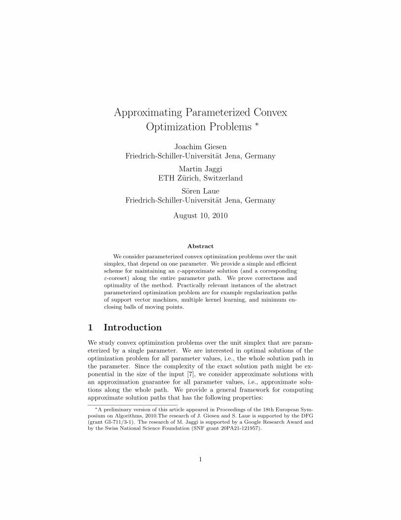
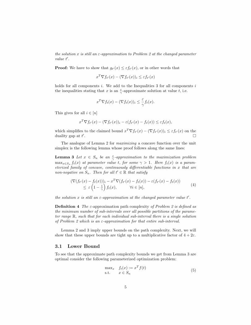
where f(t) = (f0(t), . . . , fn−1(t)) is a vector of functions and fi(t) is defined asfollows

fi(t) =

0, for t < iε′

t− iε′, for iε′ ≤ t < 1 + iε′

−t+ 2 + iε′, for 1 + iε′ ≤ t ≤ 2 + iε′

0, for 2 + iε′ < t

for some arbitrary fixed ε′ > 0 and n > 1/ε′. See Figure 1 for an illustration ofthe function fi(t).

i · ε′ 1 + i · ε′ 2 + i · ε′

1

t

Figure 1: Function fi(t).

Each of the fi(t) attains its maximum 1 at t = 1+iε′. Since ft(x) is linear inx it is also concave in x for every fixed t. Hence, it is an instance of Problem 2.Let us now consider the interval t ∈ [1, 2]. In this interval consider the pointsti := 1+ iε′, for i = 0, . . . , b1/ε′c. At each of these points it holds that fi(ti) = 1and all the other fj(ti) ≤ 1 − ε′ when j 6= i. Hence, the value of the optimalsolution to Problem 5 at parameter value ti is 1, and it is attained at x = ei,where ei is the i-th standard basis vector. Furthermore, for all other x ∈ Snthat have an entry at the coordinate position i that is at most 1/2 it holds thatfti(x) ≤ 1− ε′/2.

Hence, in order to have an ε-approximation for ε < ε′/2 the approximatesolution x needs to have an entry of more than 1/2 at the i-th coordinateposition. Since all entries of x sum up to 1, all the other entries are strictly lessthan 1/2 and hence this solution cannot be an ε-approximation for any otherparameter value t = tj with j 6= i. Thus, for all values of t ∈ [1, 2] one needs atleast 1/ε′ different solutions for any ε < ε′/2.

Choosing ε′ arbitrarily close to 2ε this implies that one needs at least 12ε − 1

different solutions to cover the whole path for t ∈ [1, 2].Lemma 3 gives an upper bound of 2+ε

εγγ−1 =

(2ε + 1

)γγ−1 different solutions,

since ∇ft(x) = f(t) = (fi(t))i∈[n] and∣∣∣∂fi

∂t

∣∣∣ ≤ 1,(∇(ft′(x)− ft(x))

)i≤ |t′ − t|.

Hence, this is optimal up to a factor of 4 + 2ε. Indeed, also the dependence onthe problem specific constants in Lemma 3 is tight: ’contracting’ the functionsfi(t) along the t-direction increases the Lipschitz constant of (∇ft(x))i, whichis an upper bound on the problem specific constants in Lemma 3.

6

3.2 The Weighted Sum of Two Convex Functions

We are particularly interested in a special case of Problem 2. For any twoconvex, continuously differentiable functions f (1), f (2) : Rn → R that are non-negative on Sn, we consider the weighted sum ft(x) := f (1)(x) + tf (2)(x) for areal parameter t ≥ 0. The parameterized optimization Problem 2 in this casebecomes

minx f (1)(x) + tf (2)(x)s.t. x ∈ Sn (6)

For this optimization problem we have the following corollary of Lemma 2:

Corollary 5 Let x ∈ Sn be an εγ -approximate solution to Problem 6 for some

fixed parameter value t ≥ 0, and for some γ > 1. Then for all t′ ≥ 0 that satisfy

(t′ − t)(xT∇f (2)(x)− (∇f (2)(x))i − εf (2)(x)

)≤ ε

(1− 1

γ

)ft(x), ∀i ∈ [n]

(7)solution x is an ε-approximate solution to Problem 6 at the parameter value t′.

Proof: Follows directly from Lemma 2, and ft′(x)− ft(x) = (t′ − t)f (2)(x).

This allows us to determine the entire interval of admissible parameter valuest′ such that an ε

γ -approximate solution at t is still an ε-approximate solution att′.

Corollary 6 Let x be an εγ -approximate solution to the Problem 6 for some

fixed parameter value t ≥ 0, for some γ > 1, and let

u := xT∇f (2)(x)−mini

(∇f (2)(x)

)i− εf (2)(x)

l := xT∇f (2)(x)−maxi

(∇f (2)(x)

)i− εf (2)(x),

then l ≤ u and x remains an ε-approximate solution for all 0 ≤ t′ = t + δ forthe following values of δ:

(i) If l < 0 and 0 < u, then the respective admissible values for δ are

ε

(1− 1

γ

)ft(x)l≤ δ ≤ ε

(1− 1

γ

)ft(x)u

(ii) If u ≤ 0, then δ (and thus t′) can become arbitrarily large.

(iii) If l ≥ 0, then δ can become as small as −t, and thus t′ can become 0.

Note that the ε-approximation path complexity for Problem 6 for a givenvalue of γ > 1 can be upper bounded by the minimum number of points tj ≥ 0such that the admissible intervals of ε

γ -approximate solutions xj at tj cover the

7

whole parameter interval [0,∞).

Corollary 6 immediately suggests two variants of an algorithmic framework(forward- and backward version) maintaining ε-approximate solutions over theentire parameter interval, or in other words, tracking a guaranteed ε-approximatesolution path. Note that as the internal optimizer, any arbitrary approximationalgorithm can be used here, as long as it provides an approximation guaran-tee on the relative primal-dual gap. For example the standard Frank-Wolfealgorithm [5, Algorithm 1.1] is particularly suitable as its resulting coreset so-lutions are also sparse. The forward variant is depicted in Algorithm 1 and thebackward variant in Algorithm 2.

Algorithm 1 ApproximationPath—ForwardVersion (ε, γ, tmin, tmax)1 compute an ε

γ-approximation x for ft(x) at t := tmin using a standard

optimizer.

2 do

3 u := xT∇f (2)(x)−mini(∇f (2)(x)

)i− εf (2)(x)

4 if u > 0 then

5 δ := ε(1− 1

γ

)ft(x)u

> 0

6 t := t+ δ

7 improve the (now still ε-approximate) solution x for ft(x) to an at leastεγ-approximate solution by applying steps of any standard optimizer.

8 else

9 t := tmax

10 while t < tmax

Algorithm 2 ApproximationPath—BackwardVersion (ε, γ, tmax, tmin)1 compute an ε

γ-approximation x for ft(x) at t := tmax using a standard

optimizer.

2 do

3 l := xT∇f (2)(x)−maxi(∇f (2)(x)

)i− εf (2)(x)

4 if l < 0 then

5 δ := ε(1− 1

γ

)ft(x)l

< 0

6 t := t+ δ

7 improve the (now still ε-approximate) solution x for ft(x) to an at leastεγ-approximate solution by applying steps of any standard optimizer.

8 else

9 t := tmin

10 while t > tmin

8

4 Applications

Special cases of Problem 6 or the more general Problem 2 have applications incomputational geometry and machine learning. In the following we discuss threeof these applications in more detail, namely, regularization paths of supportvector machines (SVMs), multiple kernel learning, and smallest enclosing balls oflinearly moving points. The first two applications for SVMs are special instancesof a parameterized polytope distance problem that we discuss at first.

4.1 A Parameterized Polytope Distance Problem

In the setting of Section 3.2 we consider the case f (1)(x) := xTK(1)x andf (2)(x) := xTK(2)x, for two positive semi-definite matrices K(1),K(2) ∈ Rn×n,or formally

minx f (1)(x) + tf (2)(x) = xT(K(1) + tK(2)

)x

s.t. x ∈ Sn . (8)

The geometric interpretation of this problem is as follows: let A(t) ∈ Rn×r,r ≤ n, be the unique matrix such A(t)TA(t) = K(1) + tK(2) (Cholesky decom-position). The solution x to Problem 8 is the point in the convex hull of thecolumn vectors of the matrix A(t) that is closest to the origin. Hence, Problem 8is a parameterized polytope distance problem. For the geometric interpretationof an ε-approximation in this context we refer to [9]. In the following we willconsider two geometric parameters for any fixed polytope distance problem:

Definition 7 For a positive semi-definite matrix K ∈ Rn×n, we define

ρ(K) := minx∈Sn

xTKx and R(K) := maxiKii

or in other words when considering the polytope associated with K, ρ(K) is theminimum (squared) distance to the origin, and R(K) is the largest squared normof a point in the polytope. We say that the polytope distance problem min

x∈Sn

xTKx

is separable if ρ(K) > 0.

For the parameterized Problem 8, the two quantities u and l that determinethe admissible parameter intervals in Corollary 6 and the step size in bothapproximate path algorithms take the simpler form

u = (2− ε)xTK(2)x− 2 mini

(K(2)x)i and l = (2− ε)xTK(2)x− 2 maxi

(K(2)x)i,

since ∇f (2)(x) = 2K(2)x. We can now use the following lemma to bound thepath complexity for instances of Problem 8.

Lemma 8 Let 0 < ε ≤ 1 and γ > 1. Then for any parameter t ≥ 0, the lengthof the interval [t − δ, t] with δ > 0, on which an ε

γ -approximate solution x toProblem 8 at parameter value t remains an ε-approximation, is at least

lf (ε, γ) :=ε

2

(1− 1

γ

)ρ(K(1))

R(K(2))

= Ω(ε) . (9)

9

Proof: For l = (2− ε)xTK(2)x− 2 maxi(K(2)x)i < 0, we get from Corollary 6that the length of the left interval at x is of length at least

ε

(1− 1

γ

)ft(x)−l .

For any t ≥ 0, we can lower bound

ft(x) ≥ f (1)(x) = xTK(1)x ≥ minx∈Sn

xTK(1)x = ρ(K(1)),

and for ε ≤ 1 we can upper bound

−l = 2 maxi

(K(2)x)i − (2− ε)xTK(2)x ≤ 2 maxi

(K(2)x)i,

because f (2)(x) ≥ 0. The value maxi(K(2)x)i = maxi eTi K(2)x is the inner

product between two points in the convex hull of the columns of the square rootof the positive semi-definite matrix K(2) (see the discussion at the beginning ofthis section). Let these two points be u, v ∈ Rn. Using the Cauchy-Schwarzinequality we get

maxi

(K(2)x)i = uT v ≤√||u||2||v||2 ≤ 1

2(||u||2 + ||v||2)

≤ max||u||2, ||v||2 ≤ maxx∈Sn

xTK(2)x,

where the last expression gives the norm of the longest vector with endpoint inthe convex hull of the columns of the square root of K(2). However, the largestsuch norm (in contrast to the smallest norm) is always attained at a vertex ofthe polytope, or formally maxx∈Sn

xTK(2)x = maxi eTi K(2)ei = maxiK

(2)ii =

R(K(2)). Hence, −l ≤ 2R(K(2)). Combining the lower bound for ft(x) and theupper bound for −l gives the stated bound on the interval length.

Now, to upper bound the approximation path complexity we split the domain[0,∞] into two parts: the interval [0, 1] can be covered by at most 1/lf (ε, γ) ad-missible left intervals, i.e., by at most 1/lf (ε, γ) many admissible sub-intervals.We reduce the analysis for the interval t ∈ [1,∞] to the analysis for [0, 1] byinterchanging the roles of f (1) and f (2). For any t ≥ 1, x is an ε-approximate so-lution to minx∈Sn

ft(x) := f (1)(x)+ tf (2)(x) if and only if x is an ε-approximatesolution to minx∈Sn

f ′t′(x) := t′f (1)(x) + f (2)(x) for t′ = 1t ≤ 1, because the def-

inition of an ε-approximation is invariant under scaling the objective function.Note that by allowing t = ∞ we just refer to the case t′ = 0 in the equivalentproblem for f ′t′(x) with t′ = 1

t ∈ [0, 1]. Using the lower bounds on the sub-interval lengths lf (ε, γ) and lf ′(ε, γ) (for the problem for f ′t′(x) with t′ ∈ [0, 1])

on both sub-intervals we get an upper bound of⌈

1lf (ε,γ)

⌉+⌈

1lf′ (ε,γ)

⌉on the path

complexity as is detailed in the following theorem:

10

Theorem 9 Given any 0 < ε ≤ 1 and γ > 1, and assuming that the distanceproblems associated to K(1) and K(2) are both separable, we have that the ε-approximation path complexity of Problem 8 is at most

γ

γ − 1

(R(K(2))

ρ(K(1))

+R(K(1))

ρ(K(2))

)2ε

+ 2 = O

(1ε

).

This proof of the path complexity immediately implies a bound on the timecomplexity of our approximation path Algorithm 1. In particular we obtaina linear running time of O

(nε2

)for computing the global solution path when

using [5, Algorithm 1.1] as the internal optimizer.There are interesting applications of this result, because it is known that

instances of Problem 8 include for example computing the solution path of asupport vector machine – as the regularization parameter changes – and alsofinding the optimal combination of two kernel matrices in the setting of kernellearning. We will discuss these applications in the following sections.

4.2 The Regularization Path of Support Vector Machines

Support Vector Machines (SVMs) are well established machine learning tech-niques for classification and related problems. It is known that most of thepractically used SVM variants are equivalent to a polytope distance problem,i.e., finding the point in the convex hull of a set of data points that is closest tothe origin [9]. In particular the so called one class SVM with `2-loss term [17,Equation (8)], and the two class `2-SVM without offset as well as with penal-ized offset, see [17, Equation (13)] for details, can be formulated as the followingpolytope distance problem

minx xT(K + 1

c1)x

s.t. x ∈ Sn (10)

where the so called kernel matrix K is an arbitrary positive semi-definite ma-trix consisting of the inner products Kij = 〈φ(pi), φ(pj)〉 of the data pointsp1, . . . , pn ∈ Rd mapped into some kernel feature space φ(Rd). The parame-ter c (= 1/t) is called the regularization parameter, and controls the trade-offbetween the regularization and the loss term in the objective function. Se-lecting the right regularization parameter value and by that balancing betweenlow model complexity and overfitting is a very important problem for SVMsand machine learning methods in general and highly influences the predictionaccuracy of the method.

Problem 10 is a special case of Problem 8 with K(2) = 1, and in this case thequantities u and l (used in Corollary 6 and the approximate path Algorithm 1and Algorithm 2 now have the even simpler form

u = (2− ε)xTx− 2 minixi and l = (2− ε)xTx− 2 max

ixi,

11

and from Lemma 8 we get the following corollary for the complexity of anapproximate regularization path, i.e., the approximation path complexity forProblem 10

Corollary 10 Given 0 < ε ≤ 1 and γ > 1, and assuming that the distanceproblem associated to K is separable, we have that the ε-approximation pathcomplexity of the regularization parameter path for c ∈ [cmin,∞) is at most

γ

γ − 1R(K) + cmin

ρ(K) · cmin· 2ε

+ 2 = O

(R(K)

ρ(K)cmin · ε)

= O

(1

ε · cmin

).

Proof: As in the proof of Theorem 9, the number of admissible sub-intervalsneeded to cover the interval of parameter values t = 1

c ∈ [0, 1] can be boundedby

γ

γ − 11

ρ(K)

2ε

= O

(1ε

),

because R(1) = maxi

1ii = 1.

The interval t ∈ [1, 1/cmin] or equivalently c ∈ [cmin, 1] (and f ′c(x) = xT1x+c · xTKx) can also be analyzed following the proof of Lemma 8. Only, now webound the function value as follows

f ′c(x) = xT1x+ cxTKx ≥ cxTKx ≥ cmin minx∈Sn

xTKx = cminρ(K)

to lower bound the length of an admissible interval. Hence, the number ofadmissible intervals needed to cover [cmin, 1] is at most

γ

γ − 11

cmin

R(K)

ρ(K)

2ε.

Adding the complexities of both intervals gives the claimed complexity for theregularization path.

Of course we could also have used Theorem 9 directly, but using ρ(1) = 1n

would only give a complexity bound that is proportional to n. However, if wechoose to stay above cmin, then we can obtain the better bound as described inthe above theorem.

Globally Valid Coresets Using the above Theorem 9 for the numberO(

1ε·cmin

)of intervals of constant solutions, and combining this with the size O

(1ε

)of a

coreset at a fixed parameter value, as e.g. provided by [5, Algorithm 1.1], wecan just build the union of those individual coresets to get an ε-coreset of sizeO(

1ε2·cmin

)that is valid over the entire solution path. This means we have

upper bounded the overall number of support vectors used in a solution validover the entire parameter range c ∈ [cmin,∞). This is particularly nice as thisnumber is independent of both the number of data points and the dimension ofthe feature space, and can easily be constructed by our Algorithms 1 and 2.

In Section 5.1 we report experimental results using this algorithmic frame-work for choosing the best regularization parameter.

12

4.3 Multiple Kernel Learning

Another immediate application of the parameterized framework in the contextof SVMs is “learning” the best combination of two kernels. This is a specialcase of the multiple kernel learning problem, where the optimal kernel to beused in a SVM is not known a priori, but needs to be selected out of a set ofcandidates. This set of candidates is often chosen to be the convex hull of a fewgiven “base” kernels, see for example [3]. In our setting with two given kernelmatrices K(1),K(2), the kernel learning problem can be written as follows:

minx xT(λK(1) + (1− λ)K(2) + 1

c1)x

s.t. x ∈ Sn (11)

where 0 ≤ λ ≤ 1, is the parameter that we want to learn. To simplify thenotation, let us define the matrices K(1)

c := K(1) + 1c and K

(2)c := K(2) + 1

c .By scaling the objective function by 1/λ (where λ is assumed to be non-zero),Problem 11 can be transformed to a special case of Problem 8, where t =1−λλ (note again that the scaling does not affect our measure of primal-dual

approximation error):

minx xTK(1)c x+ t · xTK(2)

c xs.t. x ∈ Sn (12)

This again allows us to apply both approximation path Algorithms 1 and 2,and to conclude from Theorem 9 that the complexity of an ε-approximate pathfor Problem 12 for t ∈ [0,∞] is in O

(1ε

). Here the assumption that the distance

problems associated to K(1)c and K(2)

c are both separable holds trivially because1/c > 0.

In the case that we have more than two base kernels we can still apply theabove approach if we fix the weights of all kernels except one. We can thennavigate along the solution paths optimizing each kernel weight separately, andtherefore try to find total weights with a hopefully best possible cross-validationaccuracy. In Section 5.2 we report experimental results to determine the bestcombination of two kernels to achieve the highest prediction accuracy.

4.4 Minimum Enclosing Ball of Points under Linear Mo-tion

Of interest from a more theoretical point of view is the following problem. LetP = p1, . . . , pn be a set of n points in Rd. The minimum enclosing ball (MEB)problem asks to find the smallest ball containing all points of P . The dual ofthe problem can be written [13] as

maxx xT b− xTATAxs.t. x ∈ Sn (13)

where b = (bi) = (pTi pi)i∈[n] and A is the matrix whose columns are the pi.

13

Now we assume that the points each move with constant speed in a fixeddirection, i.e., they move linearly as follows

pi(t) = pi + tvi, t ∈ [0,∞)

where t can be referred to as time parameter. The MEB problem for movingpoints reads as

maxx xT b(t)− xT (P + tV )T (P + tV )xs.t. x ∈ Sn (14)

where b(t) = (bi(t)) = ((pi + tvi)T (pi + tvi))i∈[n] and P is the matrix whosecolumns are the points pi and V is the matrix whose columns are the vectors vi.Problem 14 is a special case of the maximization version of Problem 6. Again,we are interested in the whole solution path, i.e. we want to track the centerand the radius

r(t) =√xT b(t)− xT (P + tV )T (P + tV )x with x ∈ Sn optimal

of the MEB of the points pi(t) for t ∈ [0,∞) (or approximations of it). For ananalysis of an approximate solution path we make use of the following observa-tion.

Observation 1 The interval [0,∞) can be subdivided into three parts: on thefirst sub-interval r(t) is decreasing, on the second sub-interval, the radius r(t)is constant, and on the third sub-interval, the radius is increasing.

This can be seen as follows: consider the time when the radius of the MEBreaches its global minimum, just before the ball is expanding again. This is thepoint between the second and the third sub-interval. The points that cause theball to expand at this point in time will prevent the ball from shrinking againin the future since the points move linearly. Thus the radius of the MEB willincrease on the third sub-interval. By reversing the direction of time the sameconsideration leads to the observation that the radius of the MEB is decreasingon the first sub-interval.

We will consider each of the three sub-intervals individually. The second sub-interval can be treated like the standard MEB problem of non-moving points(MEB for the points vi). Hence we only have to consider the first and thethird sub-interval. We will only analyze the third sub-interval since the firstsub-interval can be treated analogously with the direction of time reversed, i.e.,the parameter t decreasing instead of increasing.

For the third sub-interval we know that the radius is increasing with time.We can shift the time parameter t such that we start with the third sub-intervalat time t = 0. Let r > 0 be the radius r(0) at time zero, i.e., we assume that theradius of the MEB never becomes zero. The case where the radius reaches 0 atsome point is actually equivalent to the standard MEB problem for non-movingpoints. Without loss of generality we can scale all the vectors vi such that the

14

MEB defined by the points vi has radius r as well, because this just meansscaling time. Without loss of generality we can also assume that the center ofthe MEB of the point sets P and V are both the origin. That is, ‖pi‖ ≤ r and‖vi‖ ≤ r. We have for ft(x) := xT b(t)− xT (P + tV )T (P + tV )x

(∇ft(x))i = (pi + tvi)T (pi + tvi)− 2(pi + tvi)T (P + tV )x= ‖pi + tvi − (P + tV )x‖2 − xT (P + tV )T (P + tV )x

and

xT∇ft(x) = xT(b(t)− 2(P + tV )T (P + tV )x

)= xT b(t)− 2xT (P + tV )T (P + tV )x

and hence

(∇ft(x))i − xT∇ft(x)= ‖pi + tvi − (P + tV )x‖2 − (xT b(t)− xT (P + tV )T (P + tV )x

)= ‖pi + tvi − (P + tV )x‖2 − ft(x)

The partial derivative with respect to t of the above expression satisfies

∂

∂t

((∇ft(x))i − xT∇ft(x)

)=

∂

∂t

(‖pi + tvi − (P + tV )x‖2 − xT b(t) + xT (P + tV )T (P + tV )x)

= 2(pi + tvi − (P + tV )x)T (vi − V x)− ∂

∂t

∑xi‖pi + tvi‖2 + 2((P + tV )x)TV x

= 2(pi + tvi − (P + tV )x)T (vi − V x)−∑

2xi(pi + tvi)T vi + 2((P + tV )x)TV x

Using the Cauchy-Schwarz inequality, x ∈ Sn, i.e.,∑ni=1 xi = 1, xi ≥ 0, and the

fact that ‖pi‖, ‖vi‖ ≤ r we get∣∣∣∣ ∂∂t (∇ft(x))i − xT∇ft(x)∣∣∣∣ ≤ 2(r + tr + (r + tr))2r + 2(r + tr)r + 2(r + tr)r

= 12r2(1 + t)

Hence, by the mean value theorem we have that

(∇ft+δ(x)−∇ft(x))i − xT (∇ft+δ(x))−∇ft(x)) ≤ 12r2(1 + t+ δ)δ.

From a similar calculation as above we obtain

|ft+δ(x)− ft(x)| ≤ 4r2(1 + t+ δ)δ.

Now we can apply Lemma 3. Inequality 4 here simplifies to

12r2(1 + t+ δ)δ + ε4r2(1 + t+ δ)δ ≤ ε(

1− 1γ

)r2

15

since ft(x) ≥ r2. Assuming ε ≤ 1, we can set δ = ε32

(1− 1

γ

)for t, t+ δ ∈ [0, 1].

For the interval of t, t+ δ ∈ [1,∞) we apply the same trick as before and reduceit to the case of t, t+ δ ∈ [0, 1] by interchanging the roles of P and V . A shortcomputation shows that an ε-approximation x at time t ≥ 1 for the originaloptimization problem

maxx xT b(t)− xT (P + tV )T (P + tV )xs.t. x ∈ Sn

is an ε-approximation for the optimization problem

maxx xT b′(t′)− xT (t′P + V )T (t′P + V )xs.t. x ∈ Sn

at time t′ = 1/t, where b′(t′) = (b′i(t′)) = ((t′pi + vi)T (t′pi + vi))i∈[n], i.e., the

roles of P and V have been interchanged. This is again due to the fact that therelative approximation guarantee is invariant under scaling. Summing the pathcomplexities for all three sub-intervals that were considered in Observation 1,we conclude with the following theorem on the approximation path complexityfor the minimum enclosing ball problem under linear motion:

Theorem 11 The ε-approximation path complexity of the minimum enclosingball Problem 14 for parameter t ∈ [0,∞) is at most

2 · 32γ

γ − 11ε

+ 1 + 2 · 32γ

γ − 11ε

= O

(1ε

).

Since for the static MEB Problem 13, coresets of size O( 1ε ) exist, see [4], we

obtain the following corollary to Theorem 11.

Corollary 12 There exists an ε-coreset of size O( 1ε2 ) for Problem 14 that is

globally valid under the linear motion, i.e., valid for all t ≥ 0.

The only other result known in this context is the existence of coresets ofsize 2O( 1

ε2 log 1ε ) that remain valid under polynomial motions [2], and earlier, [1]

have already proven the existence of coresets of size O(1/ε2d) for the extentproblem for moving points in Rd, which includes the MEB problem as a specialcase.

5 Experimental Results

The parameterized framework from Section 3 is also useful in practice. Forsupport vector machines and multiple kernel learning, we have implementedthe approximation path Algorithms 1 and 2 in Java. As the internal blackboxoptimization procedure in lines 1 and 7, we used the coreset variants [9] of thestandard Gilbert’s [10] and MDM [14] algorithms.

16

We have tested our implementations on the following standard binary clas-sification datasets from the UCI repository1: ionosphere (n = 280, d = 34),breast-cancer (n = 546, d = 10), and MNIST 4k (n = 4000, d = 780). Thetimings were obtained by our single-threaded Java 6 implementation of MDM,using kernels but no caching of kernel evaluations, on an Intel C2D 2.4 GHzprocessor.

5.1 The Regularization Path of Support Vector Machines

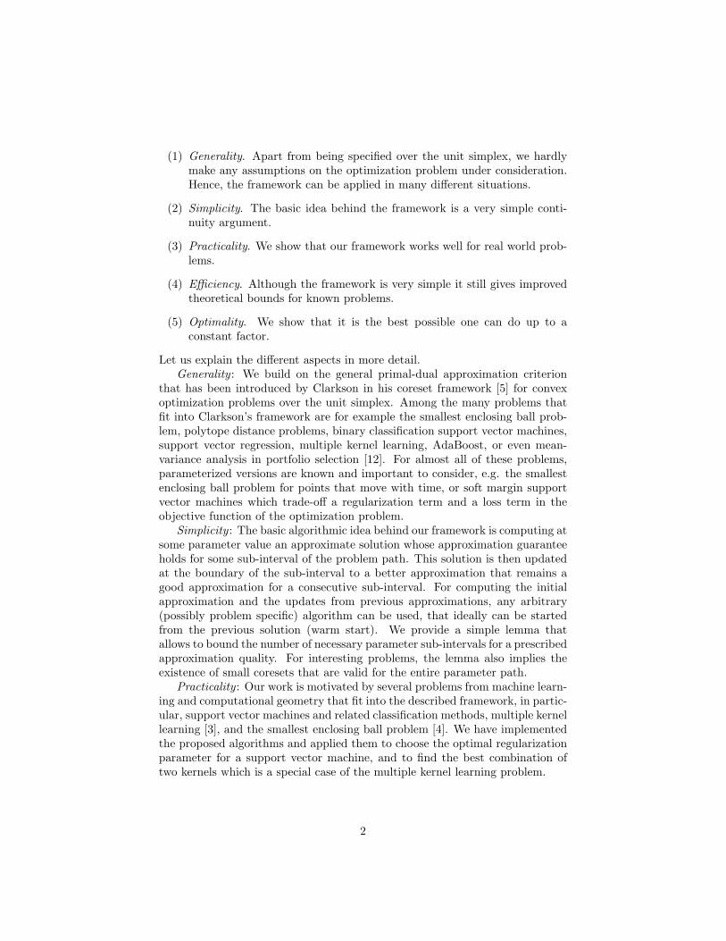
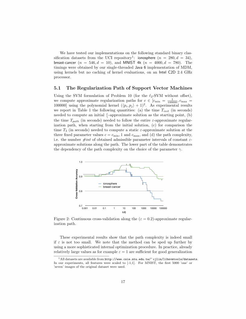
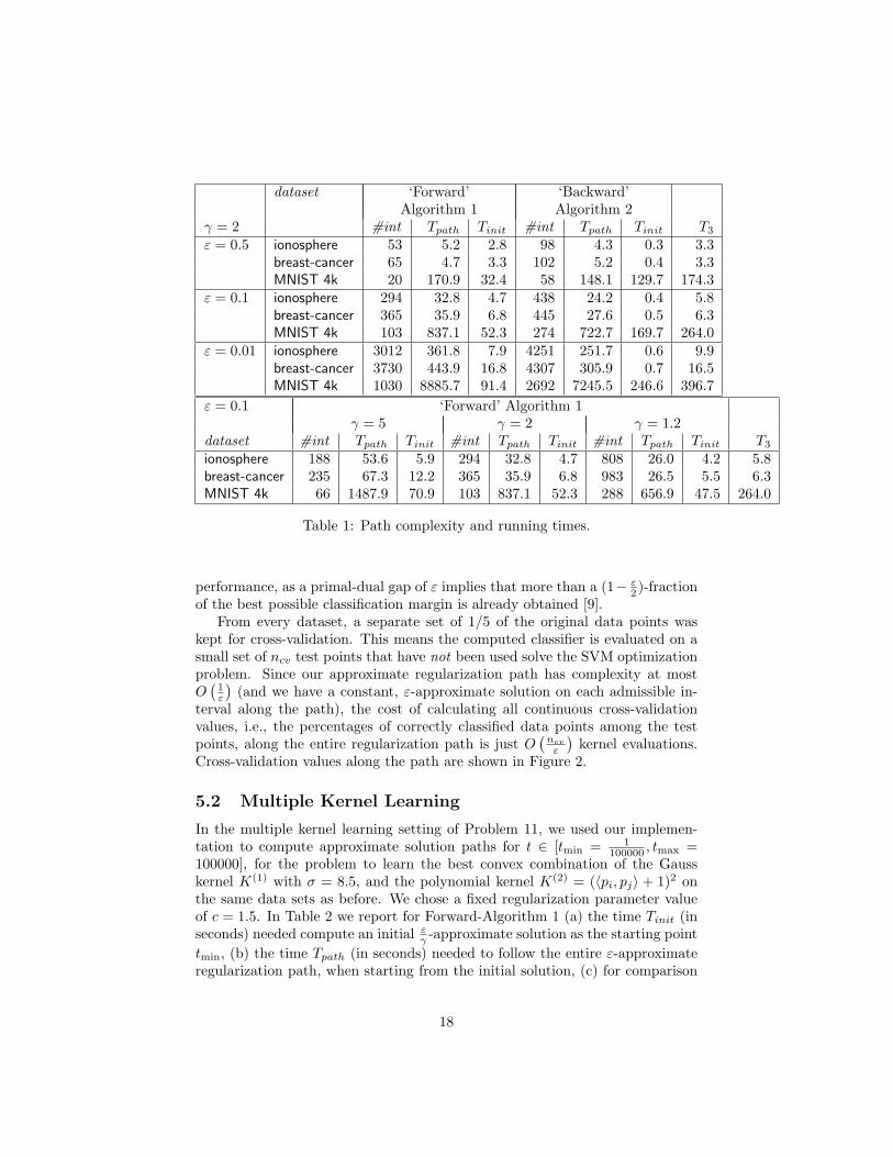
Using the SVM formulation of Problem 10 (for the `2-SVM without offset),we compute approximate regularization paths for c ∈ [cmin = 1

100000 , cmax =100000] using the polynomial kernel (〈pi, pj〉 + 1)2. As experimental resultswe report in Table 1 the following quantities: (a) the time Tinit (in seconds)needed to compute an initial ε

γ -approximate solution as the starting point, (b)the time Tpath (in seconds) needed to follow the entire ε-approximate regular-ization path, when starting from the initial solution, (c) for comparison thetime T3 (in seconds) needed to compute a static ε-approximate solution at thethree fixed parameter values c = cmin, 1 and cmax, and (d) the path complexity,i.e. the number #int of obtained admissible parameter intervals of constant ε-approximate solutions along the path. The lower part of the table demonstratesthe dependency of the path complexity on the choice of the parameter γ.

0.7

0.8

0.9

1.0

0.001 0.01 0.1 1 10 100 1000 10000 100000

Cro

ss-V

alid

ati

on

Ac

cu

rac

y

1/C

ionospherebreast-cancer

Figure 2: Continuous cross-validation along the (ε = 0.2)-approximate regular-ization path.

These experimental results show that the path complexity is indeed smallif ε is not too small. We note that the method can be sped up further byusing a more sophisticated internal optimization procedure. In practice, alreadyrelatively large values as for example ε = 1 are sufficient for good generalization

1All datasets are available from http://www.csie.ntu.edu.tw/~ cjlin/libsvmtools/datasets.In our experiments, all features were scaled to [-1,1]. For MNIST, the first 5000 ’one’ or’seven’ images of the original dataset were used.

17

dataset ‘Forward’ ‘Backward’Algorithm 1 Algorithm 2

γ = 2 #int Tpath Tinit #int Tpath Tinit T3

ε = 0.5 ionosphere 53 5.2 2.8 98 4.3 0.3 3.3breast-cancer 65 4.7 3.3 102 5.2 0.4 3.3MNIST 4k 20 170.9 32.4 58 148.1 129.7 174.3

ε = 0.1 ionosphere 294 32.8 4.7 438 24.2 0.4 5.8breast-cancer 365 35.9 6.8 445 27.6 0.5 6.3MNIST 4k 103 837.1 52.3 274 722.7 169.7 264.0

ε = 0.01 ionosphere 3012 361.8 7.9 4251 251.7 0.6 9.9breast-cancer 3730 443.9 16.8 4307 305.9 0.7 16.5MNIST 4k 1030 8885.7 91.4 2692 7245.5 246.6 396.7

ε = 0.1 ‘Forward’ Algorithm 1γ = 5 γ = 2 γ = 1.2

dataset #int Tpath Tinit #int Tpath Tinit #int Tpath Tinit T3

ionosphere 188 53.6 5.9 294 32.8 4.7 808 26.0 4.2 5.8breast-cancer 235 67.3 12.2 365 35.9 6.8 983 26.5 5.5 6.3MNIST 4k 66 1487.9 70.9 103 837.1 52.3 288 656.9 47.5 264.0

Table 1: Path complexity and running times.

performance, as a primal-dual gap of ε implies that more than a (1− ε2 )-fraction

of the best possible classification margin is already obtained [9].From every dataset, a separate set of 1/5 of the original data points was

kept for cross-validation. This means the computed classifier is evaluated on asmall set of ncv test points that have not been used solve the SVM optimizationproblem. Since our approximate regularization path has complexity at mostO(

1ε

)(and we have a constant, ε-approximate solution on each admissible in-

terval along the path), the cost of calculating all continuous cross-validationvalues, i.e., the percentages of correctly classified data points among the testpoints, along the entire regularization path is just O

(ncv

ε

)kernel evaluations.

Cross-validation values along the path are shown in Figure 2.

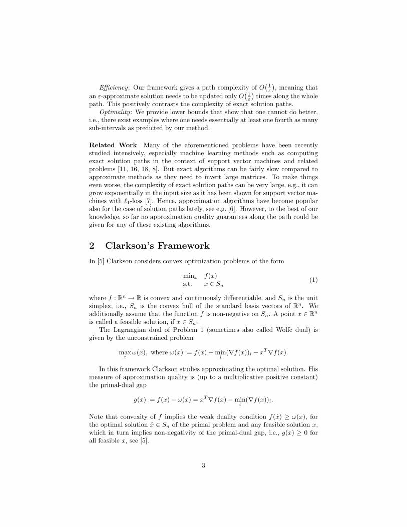
5.2 Multiple Kernel Learning

In the multiple kernel learning setting of Problem 11, we used our implemen-tation to compute approximate solution paths for t ∈ [tmin = 1

100000 , tmax =100000], for the problem to learn the best convex combination of the Gausskernel K(1) with σ = 8.5, and the polynomial kernel K(2) = (〈pi, pj〉 + 1)2 onthe same data sets as before. We chose a fixed regularization parameter valueof c = 1.5. In Table 2 we report for Forward-Algorithm 1 (a) the time Tinit (inseconds) needed compute an initial εγ -approximate solution as the starting pointtmin, (b) the time Tpath (in seconds) needed to follow the entire ε-approximateregularization path, when starting from the initial solution, (c) for comparison

18

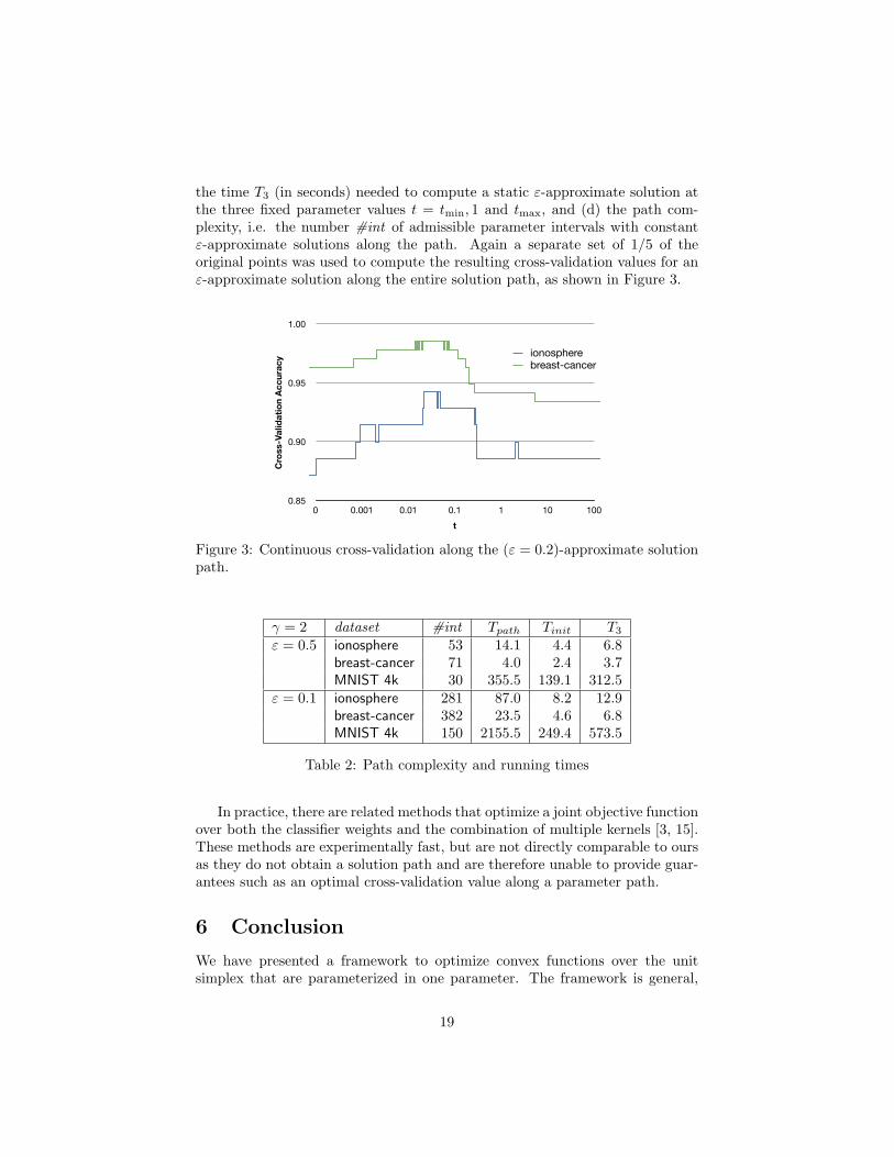
the time T3 (in seconds) needed to compute a static ε-approximate solution atthe three fixed parameter values t = tmin, 1 and tmax, and (d) the path com-plexity, i.e. the number #int of admissible parameter intervals with constantε-approximate solutions along the path. Again a separate set of 1/5 of theoriginal points was used to compute the resulting cross-validation values for anε-approximate solution along the entire solution path, as shown in Figure 3.

0.85

0.90

0.95

1.00

0 0.001 0.01 0.1 1 10 100

Cro

ss-V

alid

ati

on

Ac

cu

rac

y

t

ionospherebreast-cancer

Figure 3: Continuous cross-validation along the (ε = 0.2)-approximate solutionpath.

γ = 2 dataset #int Tpath Tinit T3

ε = 0.5 ionosphere 53 14.1 4.4 6.8breast-cancer 71 4.0 2.4 3.7MNIST 4k 30 355.5 139.1 312.5

ε = 0.1 ionosphere 281 87.0 8.2 12.9breast-cancer 382 23.5 4.6 6.8MNIST 4k 150 2155.5 249.4 573.5

Table 2: Path complexity and running times

In practice, there are related methods that optimize a joint objective functionover both the classifier weights and the combination of multiple kernels [3, 15].These methods are experimentally fast, but are not directly comparable to oursas they do not obtain a solution path and are therefore unable to provide guar-antees such as an optimal cross-validation value along a parameter path.

6 Conclusion

We have presented a framework to optimize convex functions over the unitsimplex that are parameterized in one parameter. The framework is general,

19

simple and has been proven to be practical on a number of machine learningproblems. Although it is simple it still provides improved theoretical bounds onknown problems. In fact, we showed that our method is optimal up to a smallconstant factor.

References

[1] Pankaj Agarwal, Sariel Har-Peled, and Kasturi Varadarajan. Approximat-ing extent measures of points. Journal of the ACM, 51(4):606–635, 2004.

[2] Pankaj Agarwal, Sariel Har-Peled, and Hai Yu. Embeddings of surfaces,curves, and moving points in euclidean space. SCG ’07: Proceedings of theTwenty-third Annual Symposium on Computational Geometry, 2007.

[3] Francis Bach, Gert Lanckriet, and Michael Jordan. Multiple kernel learn-ing, conic duality, and the smo algorithm. ICML ’04: Proceedings of theTwenty-first International Conference on Machine Learning, 2004.

[4] Mihai Badoiu and Kenneth L. Clarkson. Optimal core-sets for balls. Com-putational Geometry: Theory and Applications, 40(1):14–22, 2007.

[5] Kenneth L. Clarkson. Coresets, sparse greedy approximation, and thefrank-wolfe algorithm. SODA ’08: Proceedings of the Nineteenth AnnualACM-SIAM Symposium on Discrete Algorithms, 2008.

[6] Jerome Friedman, Trevor Hastie, Holger Hofling, and Robert Tibshi-rani. Pathwise coordinate optimization. The Annals of Applied Statistics,1(2):302–332, 2007.

[7] Bernd Gartner, Joachim Giesen, and Martin Jaggi. An exponential lowerbound on the complexity of regularization paths. arXiv, cs.LG, 2009.

[8] Bernd Gartner, Joachim Giesen, Martin Jaggi, and Torsten Welsch. Acombinatorial algorithm to compute regularization paths. arXiv, cs.LG,2009.

[9] Bernd Gartner and Martin Jaggi. Coresets for polytope distance. SCG ’09:Proceedings of the 25th Annual Symposium on Computational Geometry,2009.

[10] Elmer G Gilbert. An iterative procedure for computing the minimum ofa quadratic form on a convex set. SIAM Journal on Control, 4(1):61–80,1966.

[11] Trevor Hastie, Saharon Rosset, Robert Tibshirani, and Ji Zhu. The entireregularization path for the support vector machine. The Journal of MachineLearning Research, 5:1391 – 1415, 2004.

20

[12] Harry Markowitz. Portfolio selection. The Journal of Finance, 7(1):77–91,Mar 1952.

[13] Jirı Matousek and Bernd Gartner. Understanding and Using Linear Pro-gramming (Universitext). Springer-Verlag New York, Inc., Secaucus, NJ,USA, 2006.

[14] B. Mitchell, V. Dem’yanov, and V. Malozemov. Finding the point of apolyhedron closest to the origin. SIAM Journal on Control, Jan 1974.

[15] A Rakotomamonjy, F Bach, and S Canu. Simplemkl. Journal of MachineLearning Research, 9, 2008.

[16] Saharon Rosset and Ji Zhu. Piecewise linear regularized solution paths.Annals of Statistics, 35(3):1012–1030, 2007.

[17] Ivor W. Tsang, James T. Kwok, and Pak-Ming Cheung. Core vector ma-chines: Fast svm training on very large data sets. Journal of MachineLearning Research, 6:363–392, 2005.

[18] Z Wu, A Zhang, C Li, and A Sudjianto. Trace solution paths for svms viaparametric quadratic programming. KDD ’08 DMMT Workshop, 2008.

21