Embed Size (px)
Citation preview
European Journal of Operational Research 234 (2014) 641–649
Contents lists available at ScienceDirect
European Journal of Operational Research
journal homepage: www.elsevier .com/locate /e jor
Discrete Optimization
Approximation algorithms for deterministic continuous-reviewinventory lot-sizing problems with time-varying demand
0377-2217/$ - see front matter � 2013 Elsevier B.V. All rights reserved.http://dx.doi.org/10.1016/j.ejor.2013.09.037
⇑ Corresponding author. Tel.: +33 4 76 57 47 46.E-mail addresses: [email protected] (G. Massonnet), jean-philippe.
[email protected] (J.-P. Gayon), [email protected] (C. Rapine).
G. Massonnet a, J.-P. Gayon a,⇑, C. Rapine b
a Grenoble-INP/UJF-Grenoble 1/CNRS, G-SCOP UMR5272 Grenoble, F-38031, Franceb Université de Lorraine, Laboratoire LGIPM, île du Saulcy, 57045 Metz Cedex 1, France
a r t i c l e i n f o a b s t r a c t
Article history:Received 23 July 2012Accepted 22 September 2013Available online 9 October 2013
Keywords:Inventory theoryApproximation algorithmsContinuous-review policyDeterministic model
This work deals with the continuous time lot-sizing inventory problem when demand and costs aretime-dependent. We adapt a cost balancing technique developed for the periodic-review version of ourproblem to the continuous-review framework. We prove that the solution obtained costs at most twicethe cost of an optimal solution. We study the numerical complexity of the algorithm and generalize thepolicy to several important extensions while preserving its performance guarantee of two. Finally, wepropose a modified version of our algorithm for the lot-sizing model with some restricted settings thatimproves the worst-case bound.
� 2013 Elsevier B.V. All rights reserved.
1. Introduction
The Economic Order Quantity (EOQ) problem deals with asingle location that faces a demand of constant rate k. Placing anorder incurs a fixed order cost K and a linear order cost c whileholding an inventory unit incurs a cost h per unit of time. The goalis to determine a continuous-review policy of minimal cost. Thisproblem has been solved for a long time by Harris (1913) in theearly twentieth century and popularized by Wilson (1934). Sincethen, many extensions and variations have been studied includingproduction capacity, backorders, perishability, multi-echelonsystems (see e.g. Zipkin (2000) for a state of the art).
One of the important limitations of the EOQ model is theassumption of time-independent parameters. In particular, itassumes a constant demand rate k, which is not realistic in manypractical situations. Many authors relax this assumption andconsider a more general model with time-varying demand ratek(t). However they only solve the problem under very restrictiveassumptions. Resh et al. (1976) consider a time proportionaldemand rate (k(t) = at) with time-independent cost parameters.Later, Donaldson (1977) proposes an optimal policy for a linear de-mand rate (k(t) = at + b) and Barbosa and Friedman (1978) general-ize to power-form demand rates (k(t) = atb, b > �2). This result isthen extended by Henery (1979) to increasing log-concave demandpatterns and Hariga (1994) who studies a more general model forany monotonic log-concave demand rate when shortages are al-
lowed. Finally, Henery (1990) focuses on non-monotonic demandpatterns in the special case of cyclic demands.
These papers use a similar general approach that consists infinding the optimal policy for a fixed number of orders over theplanning horizon, then to determine the optimal number of ordersminimizing the total cost. This concept has been studied and gen-eralized by Benkherouf and Gilding (2009), who show that theoptimal cost over a finite planning horizon is a convex functionof the number of orders. However, this method requires specificproperties on the cost function and therefore the papers mentionedabove restrict their attention to specific demand patterns andtime-independent cost parameters. There is no general techniqueto determine an optimal continuous-review policy for time-vary-ing parameters without the restrictive assumptions discussedabove.
As the problem is difficult for more general demand patterns,the literature proposes several heuristics such as the greedy (ormyopic) approach. Silver (1979) introduces a heuristic where thelength of a replenishment cycle is chosen such that the averagecost is minimized (locally) on the replenishment cycle. This heuris-tic is inspired from the well known Silver and Meal (1973) heuris-tic designed for a periodic-review setting. Another heuristic,widely used in practice, consists of averaging the demand rateand apply the EOQ formula with the average demand to computethe order times. Goyal and Giri (2003) consider an extension ofSilver (1979) with backorders and time-varying demand rate k(t),production rate l(t) and deterioration rate h(t). They also use agreedy approach, optimizing the average cost on each cycle ratherthan globally. Many other heuristics and extensions have beenconsidered in the literature. We refer the reader to Goyal and Giri
642 G. Massonnet et al. / European Journal of Operational Research 234 (2014) 641–649
(2001) and Bakker et al. (2012) for a review of deteriorating-inven-tory models with time-varying demand and to Teng et al. (2007)for some references on the Economic Production Quantity (EPQ)model with time-varying demand.
An important heuristic discretizes the time horizon and use dy-namic programming techniques to solve the corresponding peri-odic-review problem. Indeed, there exists several polynomialtime algorithms that are optimal for the periodic-review lot-sizingproblem. In the discrete time version, the planning horizon is di-vided into n periods. In each period a demand occurs and an ordercan be placed to replenish the stock. Wagner and Whitin (1958)present an algorithm of complexity O(n2), while Aggarwal and Park(1993) propose a O(n) algorithm to solve this problem using Mongearrays. However, it is very unlikely that the optimal solution for thediscretized problem matches an optimal policy for the originalcontinuous-review version.
More generally, the previous heuristics have an importantdrawback: They can perform arbitrarily bad (i.e. no guarantee ofperformance has been proven). Even in the periodic-review setting,Axsäter (1982) shows that the heuristic of Silver and Meal (1973)can perform arbitrarily bad. That is, on some instances, the costof the heuristic is arbitrary large compared to the cost of the opti-mal policy. Similarly, the EOQ heuristic (that averages the demandand uses the EOQ formula) is also shown to perform arbitrarily bad(see Bitran et al., 1984), even if the average demand is recalculatedwhenever an order is placed.
In this paper, we aim to derive tractable policies for the contin-uous lot-sizing problem with time-varying parameters that haveprovable performance guarantees. A policy is said to have a perfor-mance guarantee (or a worst-case guarantee) of a if its cost is atmost a times the cost of an optimal policy. In the periodic-reviewsetting with time-varying demand, Axsäter (1982) shows that apolicy that balances holding and set-up costs in each replenish-ment cycle has a performance guarantee of two. Bitran et al.(1984) extend the results of Axsäter to the case with time-varyingholding costs. Recently, Van den Heuvel and Wagelmans (2010)have proven that in fact this worst-case guarantee cannot beimproved for online heuristics, i.e. procedures that use a forwardinduction mechanism and cannot modify their past ordering peri-ods. In addition, the authors propose a systematic way to constructproblem instances for which such heuristics reach their worst-casebound.
In this paper, we apply the ideas of cost balancing introducedby Bitran et al. (1984) to the continuous-review problem andprove that the performance guarantee of two remains valid forthis problem. We then show that the ideas developed are quitegeneric and can be extended to several important models fromthe inventory literature (production rate, deterioration rate,non-linear holding costs, models with shortages, time-varying or-der costs) while preserving the performance guarantee. We alsoimprove the performance guarantee to 3/2, with some additionalassumptions.
Note that Hariga (1996) applies a similar cost balancing tech-nique to the time-varying demand model with shortages and com-pares its performances to several other heuristics widely used inpractice. Although his study presents numerical experiments andcompare the performances of the different techniques, it focuseson time-independent cost parameters. Moreover, the theoreticalperformance and complexity are not discussed in his paper. Thus,to the best of our knowledge, this paper is the first to derive algo-rithms and prove their guarantee of performance for lot-sizing prob-lems with time-varying parameters in a continuous-time setting.
The rest of the paper is organized as follows: in Section 2, weformally introduce the basic lot-sizing problem and useful nota-tions to describe the solutions and prove their guarantee. Section 3explains how to adapt the balancing policy of Bitran et al. (1984)
for a continuous-time setting and prove that the resulting policypreserves the performance guarantee of 2. In Section 4, we intro-duce several extensions to the lot-sizing model and show howthe balancing algorithm can be modified to solve them. Finally,we generalize the concept of cost balancing to present a new policyfor the lot-sizing model and prove its worst-case guarantee is 1.5 inSection 5.
2. Assumptions and notations
We consider a single location that faces a continuous demandwith rate k(t) at time t. We denote by Kðs; tÞ ¼
R ts kðuÞdu the cumu-
lated demand over [s, t]. Holding an inventory unit at time t incursa cost h(t) per unit of time. We assume that k(�) and h(�) are piece-wise continuous functions. Placing an order at time t incurs a fixedorder cost (or set-up cost) K(t) and a linear order cost c(t).
The inventory level at time t is denoted by x(t). The inventorylevel at time 0, before placing the first order, is denoted by x0.For the majority of the models presented in this paper, it is domi-nant to place the first replenishment at time t0 such that x(t0) = 0and k(t0) > 0. Hence we will assume w.l.o.g. that the following ini-tial conditions (IC) holds, unless explicitely said otherwise.
ðICÞx0 ¼ 0kð0Þ > 0
�
In what follows, a policy is defined as a set of rules to determine theordering times and quantities for each instance of the problem. Theobjective is to find a policy minimizing costs over a finite horizon[0,T] while satisfying all the demands. In particular, a policy thatachieves the lowest possible cost for any instance of the problemis said to be optimal.
Without loss of generality, we assume that the procurementleadtime is null: All demands being deterministic, a deterministicpositive leadtime simply shifts the decision earlier in time. Wenow introduce some useful notations and concepts for the rest ofthe paper. Let xp(u) be the inventory level at time u, under somepolicy P and let Cpðs; tÞ be the cost incurred by a policy P over(s, t]. More precisely, Cpðs; tÞ includes holding cost
R ts hðuÞxpðuÞdu
and set-up costs over (s, t], excluding the set-up cost at time s, ifany. Then, for any sequence a0 = 0 < a1 < � � � < an+1 = T, the total costCp of policy P over the whole time horizon can be decomposed as
Cp ¼ dP0Kð0Þ þ Cpð0; TÞ ¼ dP
0Kð0Þ þXn
i¼0
Cpðai; aiþ1Þ ð1Þ
where dP0 is equal to 1 if P orders at time 0 and 0 otherwise. Notice
that when condition (IC) is satisfied and policy P is feasible, we havenecessarily dP
0 ¼ 1. Furthermore since intervals (ai,ai+1] partition thetime horizon, Eq. (1) partitions the cost incurred by any policyaccording to the sequence (ai)i=0,. . .,n+1. In particular, the followingproposition holds.
Proposition 1. Let p be a feasible policy for the continuous-reviewproblem and let 0 = a0 < a1 < � � � < an < an+1 = T be a sequence of pointsin time. If dp
0 6 dP0 and Cpðai; aiþ1Þ 6 aCpðai; aiþ1Þ for all i = 0, . . . , n
and all feasible policy P, then p has a performance guarantee of a.
Given a policy P, a (replenishment) cycle (s, t] is defined as atime interval such that an order is placed at time s, an order isplaced at time t > s and no order is placed in between. We say thata policy satisfies the Zero Inventory Ordering property, or is ZIO, if itorders only when its inventory level is zero. Note that under a ZIOpolicy P, the quantity ordered at the beginning of a cycle (s, t] isexactly K(s, t), the cumulated demand over the cycle. Moreover,the inventory level can be easily expressed in cycle (s, t] asxp(u) = K(u, t). Hence the cumulated holding cost H(s, t) of a ZIO
G. Massonnet et al. / European Journal of Operational Research 234 (2014) 641–649 643
policy over a cycle (s, t] can be simply expressed as an integral ofholding cost and demand functions.
Hðs; tÞ ¼Z t
shðuÞKðu; tÞdu
Note that since h(�) and K(�, �) are both nonnegative piecewise con-tinuous functions, H(s, �) is a nondecreasing continuous function forall s.
3. An approximation algorithm
In this section, we present the central idea of our algorithm.Roughly, the main concept is to balance in each replenishmentcycle the holding costs with the fixed order cost. For ease of under-standing, we first make similar assumptions as Bitran et al. (1984)who have investigated a periodic-review version of this problem.More precisely, we assume that the fixed order cost and the linearorder cost are time-independent, that is K(t) = K and c(t) = c for allt 2 [0,T]. These assumptions will be relaxed in Section 4. Noticethat without loss of generality, we can assume c = 0 as any policyincurs a linear order cost of exactly cK(0,T) over the planning hori-zon to satisfy all the demands. Throughout the remainder of thissection, we restrict our attention to policies that respect the ZeroInventory Ordering (ZIO) property, as it is dominant for the modelwe are interested in.
3.1. The balancing policy
The concept of cost balancing is well known in the inventory lit-erature and can even be found in the classical EOQ problem, whereall parameters are time-independent. Indeed, it is well known thatfor this special case the optimal policy balances exactly the holdingcosts with the order costs.
In the time-varying setting, we introduce the balancing policy,denoted BL in what follows, which balances in each cycle thetwo parts of the cost discussed above. The BL policy is inspiredfrom the periodic-review policy proposed by Axsäter (1982) andBitran et al. (1984). In fact, it is a ZIO policy whose order timesare determined by a forward induction as follows: A first order isplaced at the last moment when the inventory is nonnegative. Ifthe BL policy places an order at time s, the next order time is thendefined as the last time t such that
Hðs; tÞ 6 K ð2Þ
Recall that H(s, t) represents the holding cost incurred by a ZIO pol-icy over cycle (s, t]. As H(s, �) is a nondecreasing continuous functionand H(s,s) = 0, inequality (2) is tight for at least one point in [s,T] ifand only if H(s,T) P K. When the latter condition is not satisfiedthen s is the last order time of the BL policy and the quantityordered at s is K(s,T), such that all the remaining demand is orderedat s. More precisely, we define the BL policy as follows:
Definition 1. The BL policy is the ZIO replenishment policy whoseorder times s1 < s2 < � � � < sn are given by Algorithm 1.
Algorithm 1. BL policy
set s1 = 0set n 1while H(sn,T) P K do
sn+1 max {t 6 T:H(sn, t) = K}n n + 1
end whilereturn (s1, . . . ,sn)
Since the BL policy is ZIO, it is completely defined by the vectorof order times (s1, . . . ,sn). By convention we set sn+1 = T. Then fori P 1, the quantity ordered by the BL policy at time si is exactlythe cumulated demand over [si,si+1], i.e. K(si,si+i).
Remark 1. Since Algorithm 1 uses a forward induction mechanismthat does not modify past decisions, the procedure can easily beapplied in a similar fashion to problems with an infinite or a rollingtime horizon.
3.2. Performance guarantee of the BL policy
The BL policy is interesting for its simplicity and for the qualityof the solution obtained. In particular, we show in this section thatthe cost of the BL policy is at most twice the cost of an optimal pol-icy. We first present a lower bound on the cost incurred by any pol-icy between two instants s < t:
Lemma 1. For any instants s < t and any feasible policy P, we haveCpðs; tÞP minfHðs; tÞ;Kg.
Proof. If policy P places an order on (s, t], clearly Cpðs; tÞP K. If noorder is placed on (s, t], the inventory level xp(s) of policy P atinstant s is at least K(s, t) to prevent stockout on [s, t]. It impliesthat for all u 2 (s, t],xp(u) P K(u, t) and thus Hpðs; tÞ ¼
R ts hðuÞ
xpðuÞdu PR t
s hðuÞKðu; tÞdu ¼ Hðs; tÞ. The results follows. h
We now use this result to state and prove the following theo-rem on the performance guarantee of the BL policy:
Theorem 1. For piece-wise continuous functions k(�) and h(�) andconstant functions K(�) and c(�), the BL policy has a worst-caseguarantee of two. That is, the cost incurred by the BL policy is at mosttwice the cost of an optimal policy.
Proof. Let P be a feasible policy for the continuous-review lot-siz-ing problem considered and let s1, . . . , sn be the sequence of ordertimes of the BL policy. We prove that on any time interval (si,si+1],the cost incurred by the BL policy is at most twice the cost incurredby P.
Since P is feasible, we clearly have from the intial condition (IC)dbl
0 ¼ dP0 ¼ 1. On the last interval (sn,T], the cost incurred by BL is
H(sn,T), which is lower than K by construction. According toLemma 1, we have
Cpðsn; TÞP min Hðsn; TÞ;Kf g ¼ Hðsn; TÞ ¼ CBLðsn; TÞ
Now consider an interval (si,si+1], with 1 6 i 6 n � 1. By construc-tion, the BL policy incurs a holding cost H(si,si+1) = K and thusCBLðsi; siþ1Þ ¼ Hðsi; siþ1Þ þ K ¼ 2K . Due to Lemma 1, any feasible pol-icy pays at least min{H(si,si+1),K} = K on (si,si+1]. In particular, wehave that Cpðsi; siþ1ÞP K and therefore
CBLðsi; siþ1Þ 6 2Cpðsi; siþ1Þ
for all i = 0, . . . , n � 1. The theorem then follows fromProposition 1. h
3.3. Numerical issues and complexity
In this section, we discuss how the order times can be com-puted by the balancing algorithm in practice. We first turn ourattention to the issue of computing the next order time t giventhe current order time s. From the definition of H(s, �), we have that
644 G. Massonnet et al. / European Journal of Operational Research 234 (2014) 641–649
H(s,s) = 0 and H(s, �) is a nondecreasing continuous function on[s,T]. Hence there exists at least one solution t 2 [s,T] to the equa-tion H(s, t) = K (unless H(s,T) < K). However, in most cases there isno analytical expression of t. One can then use classical root-find-ing algorithms, such as the bissection method, to compute anapproximate value of t. The next ordering moment t0 found by suchtechniques is such that t0 2 [t � h, t + h] for a given precision h > 0and the final complexity depends on h. For instance when usingthe bisection method, each computation of t0 requires OðlogðT=hÞÞevaluations of function H(s, �).
For some classes of functions h(�) and k(�), like polynomial,exponential, sinusoidal, the integral H(s, t) can be expressed analyt-ically. Otherwise, one can use classical numerical methods to eval-uate this integral with some precision error. In what follows, weassume that H(s, t) can be computed (exactly) in time Oð1Þ andwe only focus on the complexity of determining the order timess1, . . . , sn of the BL policy. Notice that the number of order timesof the BL policy, as for an optimal policy, may be arbitrary large(for instance considering an exponential holding cost h(t) = et).Thus the time complexity cannot be bounded in general withrespect to the instance size. For this reason we consider in whatfollows a natural restriction of the problem.
Assume that the demand function and the holding cost functionare both upper bounded on [0,T]. That is, there exists k; h such thatfor all t 2 ½0; T�; kðtÞ 6 k and hðtÞ 6 h. Then the following theoremholds:
Theorem 2. For any e > 0, the BL policy can be implemented toprovide a solution with a performance guarantee of (2 + e) usingOðc log cÞ evaluations of H(�, �), where c ¼ ð1þ 1
eÞ khK T2.
Proof. See Appendix A. h
3.4. Worst case example
We now build an instance of the problem for which the BL pol-icy reaches its worst-case bound of 2. We consider constant hold-ing and fixed ordering costs: K = h = 1. We also assume that the
horizon T is an integer. Let I ¼ST�1
i¼1 ½i� 1=T; iþ 1=T� andI0 = I \ [0,T]. We assume that the demand rate k(t) is equal to 1when t 2 I0 and to 0 otherwise.
The BL policy orders at times 0, . . . , T � 1 and incurs a total costof CBL ¼
PT�1i¼0 2K ¼ 2T. Let P denote the ZIO policy that orders at
times 0,i � 1/T for i = 1, . . . , T. The total cost incurred by P is then
Cp ¼ K þ h2TþXT�1
i¼1
K þ hT
� �þ K þ h
2T¼ T þ 1þ
XT�1
i¼1
1Tþ 1
T¼ T þ 2
and we have limT!þ1CBL=Cp ¼ 2.
4. Extensions
The previous section presents a cost balancing technique for abasic continuous lot-sizing model, but the underlying idea appearsto be rather generic. In this section, we apply this concept to sev-eral important extensions of the lot-sizing problem. Although inmost cases Algorithm 1 cannot be used directly, we adapt thepolicy to the specific settings of each extension and prove thatthe performance guarantee of two found in Section 3 remains validfor these more general models.
4.1. Nonlinear holding costs
The analysis used in Section 3 remains valid for nonlinearholding costs. We denote by h(x, t) the holding cost value at t for
holding x units in stock. The only (natural) assumption we makeis that h(x, t) is nondecreasing in x. The cumulated holding cost ofa ZIO policy over a cycle (s, t] is again denoted by H(s, t).
Essentially, one only has to check that Lemma 1 remains valid inthis context to ensure that the approximation result holds. The pol-icy we propose in this case follows exactly Algorithm 1. This policysatisfies the ZIO property, thus the same arguments as the onesused in Theorem 1 hold and the performance guarantee of 2remains valid in the general case of nonlinear holding costs.
4.2. Perishable products
In this section, we consider a model in which the inventory onhand at time t deteriorates at rate h(t), incurring a per unit deterio-ration cost a(t). In a cycle (s,s0], the inventory level x(t) satisfies the
following first-order differential equation�
dxðtÞdt þ hðtÞxðtÞ ¼ �kðtÞ
�which can be solved easily, see e.g. Goyal and Giri (2003). Note thateven though we only present our results for the simple inventorymodel derived from Section 3, this equation can also be solved withproduction rate l(t) and backorders.
The sum of holding and deterioration costs over a time interval[s,s0] for a policy P can be expressed as:
Hpðs; s0Þ ¼Z s0
s½hðtÞ þ aðtÞhðtÞ�xpðtÞdt ¼
Z s0
s
~hðtÞxpðtÞdt
where ~hðtÞ ¼ hðtÞ þ aðtÞhðtÞ. Using this modified holding costparameter, we can apply Algorithm 1 as in Section 3. The argumentsused to prove the performance guarantee of BL remain valid in thismore general context and thus the resulting algorithm is a2-approximation for the model with perishable products.
4.3. Finite production rate
The model studied in Section 3 assumes that replenishmentsare instantaneous. We now relax this assumption and focus on amodel where units are produced according to a time-dependent,piecewise continuous production rate l(�). In addition, let
lðs; s0Þ ¼R s0
s lðzÞdz ifs 6 s0
0 otherwise
(ð3Þ
denote the cumulative production capacity between instants s ands0. If a production starts at time s for q units, all units are availableon hand at time s + t such that l(s, t) = q. Each production start in-curs a time-independent fixed cost K (the nonspeculative linear pro-duction cost is omitted w.l.o.g. as before).
Although classical production models assume that the produc-tion rate l(t) is larger than the demand rate k(t), for all t, we relaxthis constraint and consider a more general situation where theonly assumption is that the production capacity is sufficient to sat-isfy the entire demand without stockout, that is l(0, t) P K(0, t) forall t.
Observe that a policy P cannot produce more than l(s, t) unitsduring a time interval [s, t]. Thus a necessary condition for P toavoid stockouts is that for any time t P s,xp(s) P K(s, t) � l(s, t).
Property 1. Let xmin(s) = maxtPs{K(s, t) � l(s, t)}. Any feasible policyP satisfies: "s 2 [0,T],xp(s) P xmin(s).
When t = s, this condition simply implies that xp(s) P 0. Accord-ing to this new definition, we modify the initial condition (IC) andassume w.l.o.g. in this model that x0 = xmin(0) and k(0) > 0.
Note that in the special case where l(t) P k(t) for all t, we havexmin(s) = 0 for all s and the ZIO property remains dominant.Consequently we focus on policies that order at time s only if theirinventory level is equal to xmin(s). In the remainder of this section,
G. Massonnet et al. / European Journal of Operational Research 234 (2014) 641–649 645
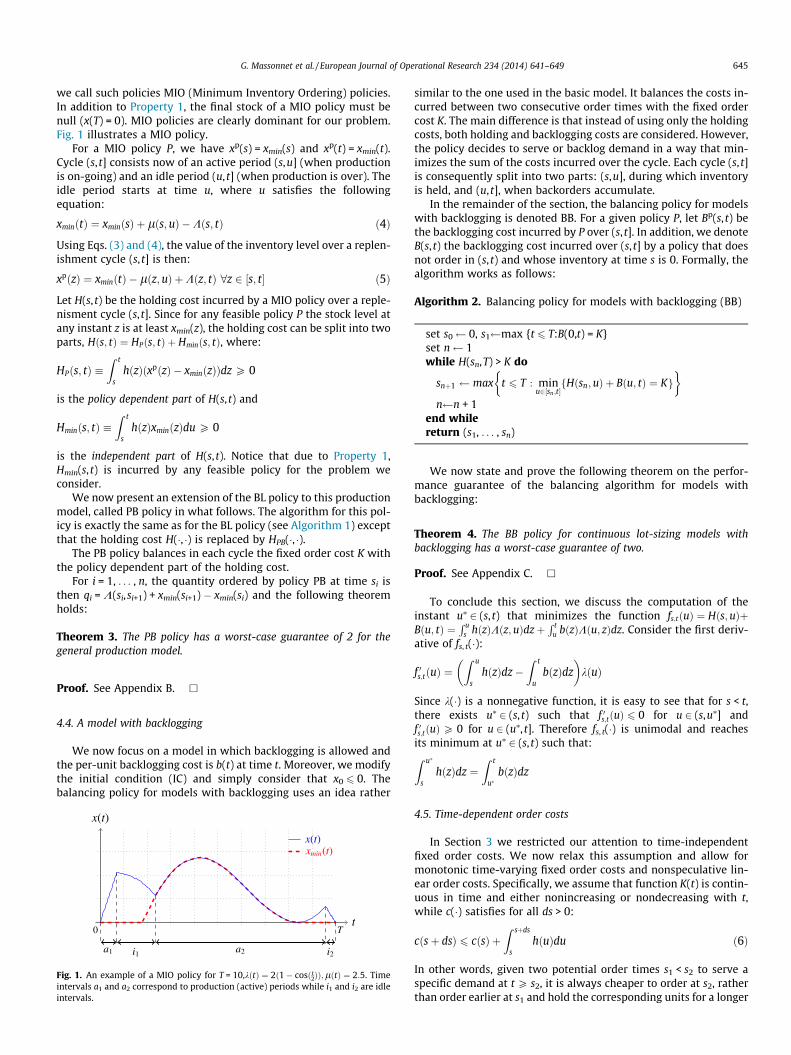
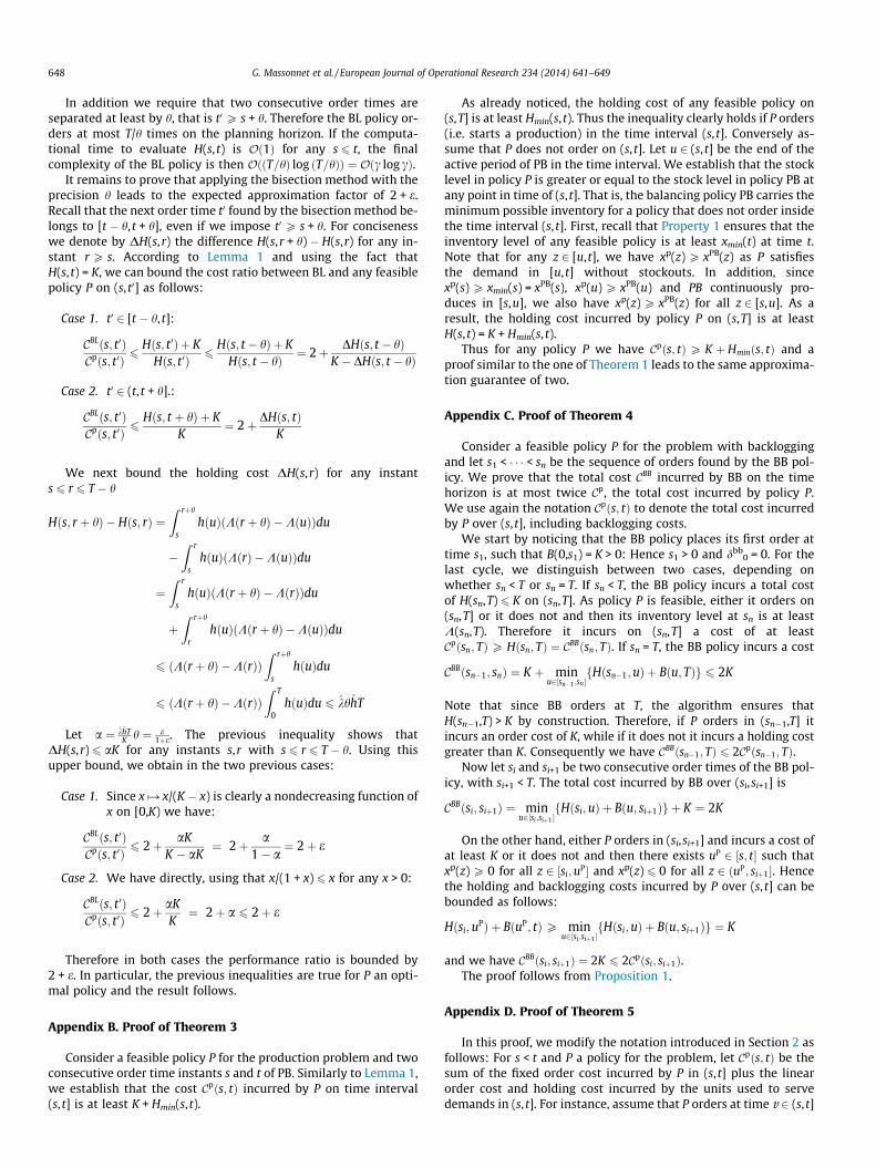
we call such policies MIO (Minimum Inventory Ordering) policies.In addition to Property 1, the final stock of a MIO policy must benull (x(T) = 0). MIO policies are clearly dominant for our problem.Fig. 1 illustrates a MIO policy.
For a MIO policy P, we have xp(s) = xmin(s) and xp(t) = xmin(t).Cycle (s, t] consists now of an active period (s,u] (when productionis on-going) and an idle period (u, t] (when production is over). Theidle period starts at time u, where u satisfies the followingequation:
xminðtÞ ¼ xminðsÞ þ lðs;uÞ �Kðs; tÞ ð4Þ
Using Eqs. (3) and (4), the value of the inventory level over a replen-ishment cycle (s, t] is then:
xpðzÞ ¼ xminðtÞ � lðz;uÞ þKðz; tÞ 8z 2 ½s; t� ð5Þ
Let H(s, t) be the holding cost incurred by a MIO policy over a reple-nisment cycle (s, t]. Since for any feasible policy P the stock level atany instant z is at least xmin(z), the holding cost can be split into twoparts, Hðs; tÞ ¼ HPðs; tÞ þ Hminðs; tÞ, where:
HPðs; tÞ �Z t
shðzÞðxpðzÞ � xminðzÞÞdz P 0
is the policy dependent part of H(s, t) and
Hminðs; tÞ �Z t
shðzÞxminðzÞdu P 0
is the independent part of H(s, t). Notice that due to Property 1,Hmin(s, t) is incurred by any feasible policy for the problem weconsider.
We now present an extension of the BL policy to this productionmodel, called PB policy in what follows. The algorithm for this pol-icy is exactly the same as for the BL policy (see Algorithm 1) exceptthat the holding cost H(�, �) is replaced by HPB(�, �).
The PB policy balances in each cycle the fixed order cost K withthe policy dependent part of the holding cost.
For i = 1, . . . , n, the quantity ordered by policy PB at time si isthen qi = K(si,si+1) + xmin(si+1) � xmin(si) and the following theoremholds:
Theorem 3. The PB policy has a worst-case guarantee of 2 for thegeneral production model.
Proof. See Appendix B. h
4.4. A model with backlogging
We now focus on a model in which backlogging is allowed andthe per-unit backlogging cost is b(t) at time t. Moreover, we modifythe initial condition (IC) and simply consider that x0 6 0. Thebalancing policy for models with backlogging uses an idea rather
x(t)
0t
T
x(t)xmin(t)
a1 i1 a2 i2
Fig. 1. An example of a MIO policy for T = 10,kðtÞ ¼ 2ð1� cosðt2ÞÞ;lðtÞ ¼ 2:5. Timeintervals a1 and a2 correspond to production (active) periods while i1 and i2 are idleintervals.
similar to the one used in the basic model. It balances the costs in-curred between two consecutive order times with the fixed ordercost K. The main difference is that instead of using only the holdingcosts, both holding and backlogging costs are considered. However,the policy decides to serve or backlog demand in a way that min-imizes the sum of the costs incurred over the cycle. Each cycle (s, t]is consequently split into two parts: (s,u], during which inventoryis held, and (u, t], when backorders accumulate.
In the remainder of the section, the balancing policy for modelswith backlogging is denoted BB. For a given policy P, let Bp(s, t) bethe backlogging cost incurred by P over (s, t]. In addition, we denoteB(s, t) the backlogging cost incurred over (s, t] by a policy that doesnot order in (s, t) and whose inventory at time s is 0. Formally, thealgorithm works as follows:
Algorithm 2. Balancing policy for models with backlogging (BB)
set s0 0, s1 max {t 6 T:B(0,t) = K}set n 1while H(sn,T) > K do
snþ1 max t 6 T : minu2½sn ;t�
Hðsn;uÞ þ Bðu; tÞ ¼ Kf g� �
n n + 1end whilereturn (s1, . . . , sn)
We now state and prove the following theorem on the perfor-mance guarantee of the balancing algorithm for models withbacklogging:
Theorem 4. The BB policy for continuous lot-sizing models withbacklogging has a worst-case guarantee of two.
Proof. See Appendix C. h
To conclude this section, we discuss the computation of theinstant u⁄ 2 (s, t) that minimizes the function fs;tðuÞ ¼ Hðs;uÞþBðu; tÞ ¼
R us hðzÞKðz;uÞdzþ
R tu bðzÞKðu; zÞdz. Consider the first deriv-
ative of fs, t(�):
f 0s;tðuÞ ¼Z u
shðzÞdz�
Z t
ubðzÞdz
� �kðuÞ
Since k(�) is a nonnegative function, it is easy to see that for s < t,there exists u⁄ 2 (s, t) such that f 0s;tðuÞ 6 0 for u 2 (s,u⁄] andf 0s;tðuÞP 0 for u 2 (u⁄, t]. Therefore fs, t(�) is unimodal and reachesits minimum at u⁄ 2 (s, t) such that:Z u�
shðzÞdz ¼
Z t
u�bðzÞdz
4.5. Time-dependent order costs
In Section 3 we restricted our attention to time-independentfixed order costs. We now relax this assumption and allow formonotonic time-varying fixed order costs and nonspeculative lin-ear order costs. Specifically, we assume that function K(t) is contin-uous in time and either nonincreasing or nondecreasing with t,while c(�) satisfies for all ds > 0:
cðsþ dsÞ 6 cðsÞ þZ sþds
shðuÞdu ð6Þ
In other words, given two potential order times s1 < s2 to serve aspecific demand at t P s2, it is always cheaper to order at s2, ratherthan order earlier at s1 and hold the corresponding units for a longer
646 G. Massonnet et al. / European Journal of Operational Research 234 (2014) 641–649
period. One can notice that inequality (6) is the continuous versionof the well-known nonspeculative assumption often encountered indiscrete lot-sizing models.
If K(�) is nonincreasing (resp. nondecreasing) the holding costH(s, t) + c(s)K(s, t) incurred over a cycle (s, t] is balanced with K(s)(resp. K(t)). The procedure is then applied in a forward or in a back-ward manner depending on the variation of K(�). Notice that Bitranet al. (1984) also define a forward and a backward method for thediscrete time problem when ordering costs are time-independent.In our case, these two algorithms are defined as follows:
Algorithm 3. Forward balancing policy for nonincreasing ordercosts
set s1 0set n 1while c(sn)K(sn,T) + H(sn,T) P K(T) do
sn+1 max {t 6 T:c(sn)K(sn, t) + H(sn, t) = K(t)}n n + 1
end whilereturn (s1, . . . , sn)
Algorithm 4. Backward balancing policy for nondecreasing ordercosts
set s0 = Tset t0 max {t 6 T:K(0, t) 6 x0}set n 0while c(t0)K(t0,sn) + H(t0,sn) P K(t0) do
sn+1 min {t P t0:c(t)K(t,sn) + H(t,sn) = K(t)}n n + 1
end whileif sn > t0 then
sn+1 min {0 6 t 6 t0:c(t)K(t0,sn) + H(t,sn) � H(t, t0) 6 K(t)}n n + 1
end ifreturn (sn, . . . , s1)
Note that in the case of the backward algorithm, the order timesare computed in a reverse order: 0 6 sn 6 � � � 6 s1 6 T. Moreover,the ZIO rule is not necessarily respected for the first order. Let x0
be the initial inventory on hand and let t0 = max{t 6 T:K(0, t) 6 x0}.If sn < t0, the quantity ordered at time sn is qn = K(t0,sn�1). All theother orders are of size qi = K(si,si�1).
Theorem 5. For time-dependent order costs, the forward (resp.backward) balancing policy has a worst-case guarantee of two whenK(�) is a continuous nonincreasing (resp. nondecreasing) function.
Proof. See Appendix D. h
5. Improvement of the performance guarantee
In this section, we present a generalization of the balancing tech-nique used in Section 3 and use it to improve the performance guar-antee from 2 to 3/2. The idea remains to balance the costs incurredover a time interval (s,s0] with order costs but we now consider thepossibility to place additional orders in the interval. We present thismodified algorithm in the simple situation of Section 3, in whichorder costs are time-independent and holding costs are linear.
5.1. A generalized balancing policy
Consider a time interval (s, t] and let k be a positive integer. Wedefine Gk(s, t) as the minimum cost over (s, t) incurred by a feasiblepolicy ordering at most k times in (s, t).
Note that a policy that minimizes the cost Gk(s, t) is ZIO. Thus fork = 0 we have G0(s, t) = H(s, t) and clearly the BL policy incurs oneach of its ordering interval (s,s0] a cost G0(s,s0). We can generalizeLemma 1 to the following result:
Lemma 2. Let k 2 N; s < t and P a feasible policy. We have
Cpðs; tÞP minfGkðs; tÞ; ðkþ 1ÞKg
Proof. The proof is immediate due to the definition of Gk. If policyP places at most k orders inside the time interval, thenCpðs; tÞP Gkðs; tÞ. Otherwise Cpðs; tÞP ðkþ 1ÞK. h
For a given positive integer k, we propose the following balanc-ing policy, denoted BLk in the remainder of this section. Its princi-ple is to balance Gk(s, t) with (k + 1)K in each of its replenishmentcycle (s, t]. That is, given an instant s, the policy computes the larg-est instant t 6 T such that Gk(s, t) 6 (k + 1)K. Notice that in this casepolicy BLk orders at instants s and t and possibly up to k times inthe interval (s, t). We call main order times the instants s and t,while the other order times in (s, t) are called secondary ordertimes. Although main and secondary orders play the same role inthe final solution, we differentiate these two types of orders to sim-plify the definition and the proof of performance of the algorithm.The following result generalizes Theorem 1:
Theorem 6. For K(�) and c(�) constant functions and h(�) and k(�) apiece-wise continuous function, the BLk policy has a worst-caseguarantee of kþ2
kþ1.
Proof. The proof is very similar to the one of Theorem 1 and onlythe main arguments are given here. Let P be a feasible policy andlet s1, . . . , sn be the sequence of the main order times of the BLk pol-icy. First notice that any feasible policy P places an order at time 0
and therefore dBLk0 ¼ dP
0 ¼ 1. Now consider an interval (si,si+1], with0 6 i 6 n � 1. By construction, the BLk policy incurs a costCblk ðsi; siþ1Þ 6 Gkðsi; siþ1Þ þ K ¼ ðkþ 2ÞK in this time interval. Dueto Lemma 2, policy P pays at least min{Gk(si,si+1),(k + 1)K} = (k + 1)K. It results that Cblk ðsi; siþ1Þ 6 kþ2
kþ1 Cpðsi; siþ1Þ. Then
consider the last interval. On [sn,T], we have Cblk ðsn; TÞ ¼ Gkðsn; TÞ,which is lower than Cpðsn; TÞ due to Lemma 2. As a consequencethe inequality Cblk ðsi; siþ1Þ 6 kþ2
kþ1 Cpðsi; siþ1Þ holds for every interval
(si,si+1] and the proof follows. h
5.2. Complexity analysis
In contrast to the balancing policy presented in Section 3, thefamily of algorithms presented in the previous section does not fallwithin the class of online heuristics defined by Van den Heuvel andWagelmans (2010) and enables us to design efficient procedures tosolve the problem introduced in Section 2. In particular, the result-ing performance guarantee can be as close as aimed to the cost ofan optimal policy. However the problem of determining (analyti-cally or numerically) the minimal cost Gk(s, t) on an interval (s, t)is likely to require a large computing effort, especially for largevalues of k. In this subsection, we first discuss the computationof Gk(s, t) for an arbitrary k. Then, for k = 1, we show that the BL1
policy can be computed in O c log cð Þ2� �
with some restrictions
on the demand and holding cost functions.
G. Massonnet et al. / European Journal of Operational Research 234 (2014) 641–649 647
5.2.1. Arbitrary kIn what follows, we assume that K(s, t) > 0. Otherwise, policy
BLk policy does not place any order (Gk(s, t) = 0). We also assumethat h(�) and k(�) are continuous functions.
When k secondary orders are placed in interval (s, t) at timesv1 6 � � � 6 vk, the inventory holding cost of a ZIO policy on interval(s, t) is
f ðv1; . . . ;vkÞ ¼Xk
i¼0
Z v iþ1
v i
hðxÞKðx;v iþ1Þdx
where v0 = s and vk+1 = t. The problem is then to minimize f with theconstraint that v0 = s 6 v1 6 � � � 6 vk+1 = t. We have for 1 6 i 6 k
@f@v iðv1; . . . ;vkÞ ¼ kðv iÞhðv i�1; v iÞ � hðv iÞKðv i; v iþ1Þ
where hðx; yÞ ¼R y
x hðtÞdt.It can be shown that the first order condition for optimality
gives for 1 6 i 6 k:
kðv iÞhðv i�1;v iÞ ¼ hðv iÞKðv i; v iþ1Þ ð7Þ
Note that this condition is necessary but not sufficient since theremay exist several solutions to Eq. (7). For time-independent holdingcost h(t) = h, condition (7) reduces to a simpler condition that wasestablished by Barbosa and Friedman (1978): (vi � vi�1)k(vi) =K(0,vi+1) �K(0,vi). However even in this restrictive setting, theproblem of solving Eq. (7) is difficult, except for very specificdemand functions (linear, power-form).
5.2.2. k = 1We now turn our attention to the case k = 1, where the problem
is to find a single optimal intermediary order. In this case, there is asingle variable v1 that we rename v for ease of understanding. If weassume that the demand function k(�) and the holding cost functionh(�) are once differentiable, we can compute the second derivativeof f(�):
d2f
dv2 ðvÞ ¼ k0ðvÞhðs;vÞ þ 2kðvÞhðvÞ � h0ðvÞKðv ; tÞ
As a consequence, f(�) is convex if and only if the following con-dition is satisfied:
k0ðvÞhðs;vÞ þ 2kðvÞhðvÞ � h0ðvÞKðv; tÞP 0 ð8Þ
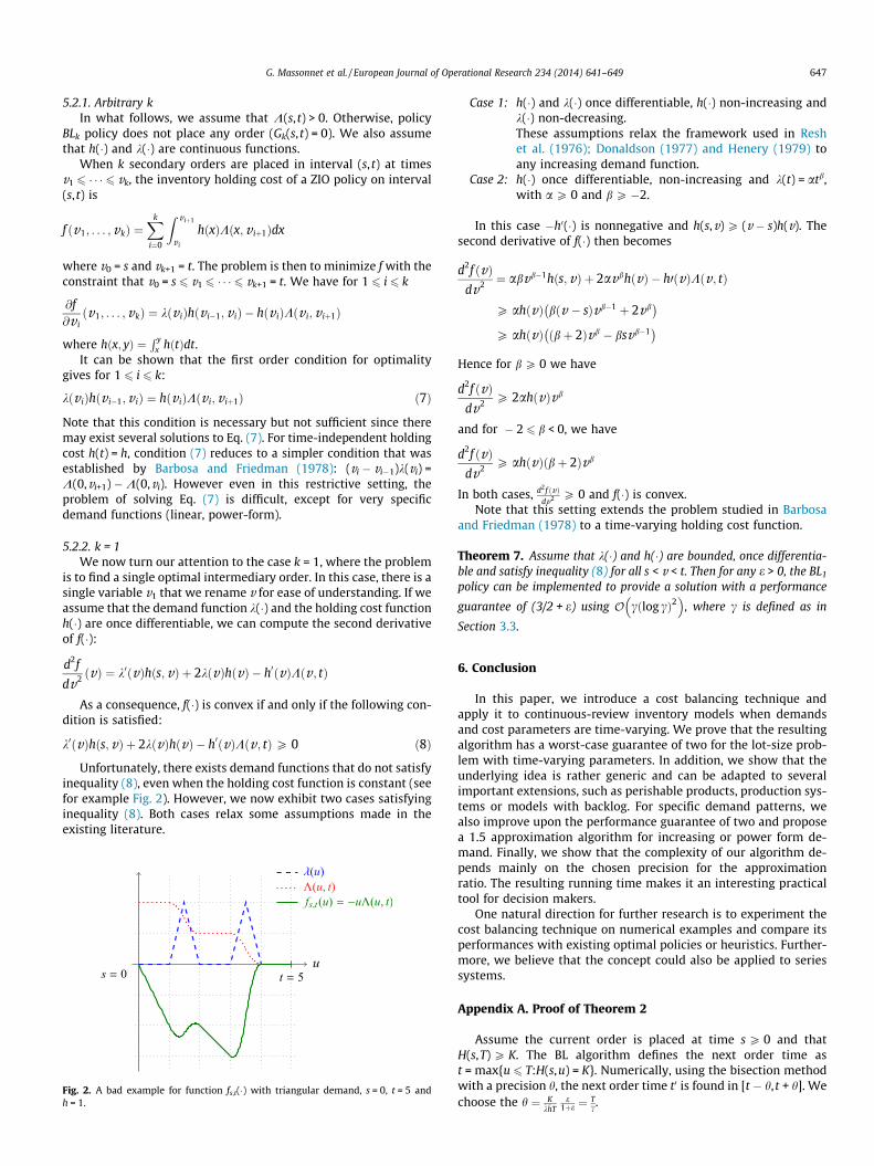
Unfortunately, there exists demand functions that do not satisfyinequality (8), even when the holding cost function is constant (seefor example Fig. 2). However, we now exhibit two cases satisfyinginequality (8). Both cases relax some assumptions made in theexisting literature.
Fig. 2. A bad example for function fs,t(�) with triangular demand, s = 0, t = 5 andh = 1.
Case 1: h(�) and k(�) once differentiable, h(�) non-increasing andk(�) non-decreasing.These assumptions relax the framework used in Reshet al. (1976); Donaldson (1977) and Henery (1979) toany increasing demand function.
Case 2: h(�) once differentiable, non-increasing and k(t) = atb,with a P 0 and b P �2.
In this case �h0(�) is nonnegative and h(s,v) P (v � s)h(v). Thesecond derivative of f(�) then becomes
d2f ðvÞdv2 ¼ abvb�1hðs;vÞ þ 2avbhðvÞ � h0ðvÞKðv; tÞ
P ahðvÞ bðv � sÞvb�1 þ 2vb�
P ahðvÞ ðbþ 2Þvb � bsvb�1� Hence for b P 0 we have
d2f ðvÞdv2 P 2ahðvÞvb
and for � 2 6 b < 0, we have
d2f ðvÞdv2 P ahðvÞðbþ 2Þvb
In both cases, d2 f ðvÞdv2 P 0 and f(�) is convex.
Note that this setting extends the problem studied in Barbosaand Friedman (1978) to a time-varying holding cost function.
Theorem 7. Assume that k(�) and h(�) are bounded, once differentia-ble and satisfy inequality (8) for all s < v < t. Then for any e > 0, the BL1
policy can be implemented to provide a solution with a performance
guarantee of (3/2 + e) using O cðlog cÞ2� �
, where c is defined as in
Section 3.3.
6. Conclusion
In this paper, we introduce a cost balancing technique andapply it to continuous-review inventory models when demandsand cost parameters are time-varying. We prove that the resultingalgorithm has a worst-case guarantee of two for the lot-size prob-lem with time-varying parameters. In addition, we show that theunderlying idea is rather generic and can be adapted to severalimportant extensions, such as perishable products, production sys-tems or models with backlog. For specific demand patterns, wealso improve upon the performance guarantee of two and proposea 1.5 approximation algorithm for increasing or power form de-mand. Finally, we show that the complexity of our algorithm de-pends mainly on the chosen precision for the approximationratio. The resulting running time makes it an interesting practicaltool for decision makers.
One natural direction for further research is to experiment thecost balancing technique on numerical examples and compare itsperformances with existing optimal policies or heuristics. Further-more, we believe that the concept could also be applied to seriessystems.
Appendix A. Proof of Theorem 2
Assume the current order is placed at time s P 0 and thatH(s,T) P K. The BL algorithm defines the next order time ast = max{u 6 T:H(s,u) = K}. Numerically, using the bisection methodwith a precision h, the next order time t0 is found in [t � h, t + h]. Wechoose the h ¼ K
khTe
1þe ¼ Tc.
648 G. Massonnet et al. / European Journal of Operational Research 234 (2014) 641–649
In addition we require that two consecutive order times areseparated at least by h, that is t0 P s + h. Therefore the BL policy or-ders at most T/h times on the planning horizon. If the computa-tional time to evaluate H(s, t) is Oð1Þ for any s 6 t, the finalcomplexity of the BL policy is then O T=hð Þ log T=hð Þð Þ ¼ Oðc log cÞ.
It remains to prove that applying the bisection method with theprecision h leads to the expected approximation factor of 2 + e.Recall that the next order time t0 found by the bisection method be-longs to [t � h, t + h], even if we impose t0 P s + h. For concisenesswe denote by DH(s,r) the difference H(s,r + h) � H(s,r) for any in-stant r P s. According to Lemma 1 and using the fact thatH(s, t) = K, we can bound the cost ratio between BL and any feasiblepolicy P on (s, t0] as follows:
Case 1. t0 2 [t � h, t]:
CBLðs; t0ÞCpðs; t0Þ 6
Hðs; t0Þ þ KHðs; t0Þ 6
Hðs; t� hÞ þ KHðs; t� hÞ ¼ 2þ DHðs; t� hÞ
K �DHðs; t� hÞ
Case 2. t0 2 (t, t + h].:
CBLðs; t0ÞCpðs; t0Þ 6
Hðs; t þ hÞ þ KK
¼ 2þ DHðs; tÞK
We next bound the holding cost DH(s,r) for any instants 6 r 6 T � h
Hðs; r þ hÞ � Hðs; rÞ ¼Z rþh
shðuÞ Kðr þ hÞ �KðuÞð Þdu
�Z r
shðuÞ KðrÞ �KðuÞð Þdu
¼Z r
shðuÞ Kðr þ hÞ �KðrÞð Þdu
þZ rþh
rhðuÞ Kðr þ hÞ �KðuÞð Þdu
6 Kðr þ hÞ �KðrÞð ÞZ rþh
shðuÞdu
6 Kðr þ hÞ �KðrÞð ÞZ T
0hðuÞdu 6 khhT
Let a ¼ khTK h ¼ e
1þe. The previous inequality shows thatDH(s,r) 6 aK for any instants s,r with s 6 r 6 T � h. Using thisupper bound, we obtain in the two previous cases:
Case 1. Since x ´ x/(K � x) is clearly a nondecreasing function ofx on [0,K) we have:
CBLðs; t0ÞCpðs; t0Þ 6 2þ aK
K � aK¼ 2þ a
1� a¼ 2þ e
Case 2. We have directly, using that x/(1 + x) 6 x for any x > 0:
CBLðs; t0ÞCpðs; t0Þ 6 2þ aK
K¼ 2þ a 6 2þ e
Therefore in both cases the performance ratio is bounded by2 + e. In particular, the previous inequalities are true for P an opti-mal policy and the result follows.
Appendix B. Proof of Theorem 3
Consider a feasible policy P for the production problem and twoconsecutive order time instants s and t of PB. Similarly to Lemma 1,we establish that the cost Cpðs; tÞ incurred by P on time interval(s, t] is at least K + Hmin(s, t).
As already noticed, the holding cost of any feasible policy on(s,T] is at least Hmin(s, t). Thus the inequality clearly holds if P orders(i.e. starts a production) in the time interval (s, t]. Conversely as-sume that P does not order on (s, t]. Let u 2 (s, t] be the end of theactive period of PB in the time interval. We establish that the stocklevel in policy P is greater or equal to the stock level in policy PB atany point in time of (s, t]. That is, the balancing policy PB carries theminimum possible inventory for a policy that does not order insidethe time interval (s, t]. First, recall that Property 1 ensures that theinventory level of any feasible policy is at least xmin(t) at time t.Note that for any z 2 [u, t], we have xp(z) P xPB(z) as P satisfiesthe demand in [u, t] without stockouts. In addition, sincexp(s) P xmin(s) = xPB(s), xp(u) P xPB(u) and PB continuously pro-duces in [s,u], we also have xp(z) P xPB(z) for all z 2 [s,u]. As aresult, the holding cost incurred by policy P on (s,T] is at leastH(s, t) = K + Hmin(s, t).
Thus for any policy P we have Cpðs; tÞP K þ Hminðs; tÞ and aproof similar to the one of Theorem 1 leads to the same approxima-tion guarantee of two.
Appendix C. Proof of Theorem 4
Consider a feasible policy P for the problem with backloggingand let s1 < � � � < sn be the sequence of orders found by the BB pol-icy. We prove that the total cost CBB incurred by BB on the timehorizon is at most twice Cp, the total cost incurred by policy P.We use again the notation Cpðs; tÞ to denote the total cost incurredby P over (s, t], including backlogging costs.
We start by noticing that the BB policy places its first order attime s1, such that B(0,s1) = K > 0: Hence s1 > 0 and dbb
0 = 0. For thelast cycle, we distinguish between two cases, depending onwhether sn < T or sn = T. If sn < T, the BB policy incurs a total costof H(sn,T) 6 K on (sn,T]. As policy P is feasible, either it orders on(sn,T] or it does not and then its inventory level at sn is at leastK(sn,T). Therefore it incurs on (sn,T] a cost of at leastCpðsn; TÞP Hðsn; TÞ ¼ CBBðsn; TÞ. If sn = T, the BB policy incurs a cost
CBBðsn�1; snÞ ¼ K þ minu2½sn�1 ;sn �
Hðsn�1;uÞ þ Bðu; TÞf g 6 2K
Note that since BB orders at T, the algorithm ensures thatH(sn�1,T) > K by construction. Therefore, if P orders in (sn�1,T] itincurs an order cost of K, while if it does not it incurs a holding costgreater than K. Consequently we have CBBðsn�1; TÞ 6 2Cpðsn�1; TÞ.
Now let si and si+1 be two consecutive order times of the BB pol-icy, with si+1 < T. The total cost incurred by BB over (si,si+1] is
CBBðsi; siþ1Þ ¼ minu2½si ;siþ1 �
Hðsi;uÞ þ Bðu; siþ1Þf g þ K ¼ 2K
On the other hand, either P orders in (si,si+1] and incurs a cost ofat least K or it does not and then there exists uP 2 ½s; t� such thatxp(z) P 0 for all z 2 ½si;uP� and xp(z) 6 0 for all z 2 ðuP; siþ1�. Hencethe holding and backlogging costs incurred by P over (s, t] can bebounded as follows:
Hðsi;uPÞ þ BðuP; tÞP minu2½si ;siþ1 �
Hðsi;uÞ þ Bðu; siþ1Þf g ¼ K
and we have CBBðsi; siþ1Þ ¼ 2K 6 2Cpðsi; siþ1Þ.The proof follows from Proposition 1.
Appendix D. Proof of Theorem 5
In this proof, we modify the notation introduced in Section 2 asfollows: For s < t and P a policy for the problem, let Cpðs; tÞ be thesum of the fixed order cost incurred by P in (s, t] plus the linearorder cost and holding cost incurred by the units used to servedemands in (s, t]. For instance, assume that P orders at time v 2 (s, t]
G. Massonnet et al. / European Journal of Operational Research 234 (2014) 641–649 649
to satisfy demands in [u, t] and at time r < s to serve demands in(s,v). Then we have
Cpðs; tÞ ¼ cðrÞKðs; vÞ þ cðvÞKðv ; tÞ þZ s
rhðxÞKðs;vÞdx
þZ v
shðxÞKðx; vÞdxþ
Z t
vhðxÞKðx; tÞdx
Note that this is an extension of the original definition of Cpð�; �Þ andthus all the previous proofs remain valid with this new definition.
We detail the proof only for the forward algorithm. Let P be afeasible policy for the problem with nonincreasing order costs.We again have dbl
0 ¼ dP0 ¼ 1 for any feasible policy P. Now let i < n
and focus on the ordering cycle (si,si+1]. We bound the costincurred by policy P over (si,si+1] as follows:
Case 1. P places an order at time u 2 (si,si+1]: It incurs an ordercost K(u) P K(si+1).
Case 2. P does not order in (si,si+1]: It incurs a holding cost of atleast H(si,si+1). Moreover, P orders the units used to servethe demands in (si,si+1] at a previous point in time s0 < si,incurring an additional linear order cost and holdingcost of cðs0Þ þ
R ss0 hðuÞdu
� Kðsi; siþ1Þ. According to Eq. (6),
we thus have:
Cpðsi; siþ1Þ ¼ cðs0Þ þZ s
s0hðuÞdu
� �Kðsi; siþ1Þ þ Hðsi; siþ1Þ
P cðsiÞKðsi; siþ1Þ þ Hðsi; siþ1ÞP Kðsiþ1Þ
Thus for any i < n and ordering cycle (si,si+1], we have:
CBLðsi; siþ1Þ ¼ 2Kðsiþ1Þ 6 2Cpðsi; siþ1Þ
Finally, one can use similar arguments to prove that we have
CBLðsn; TÞ ¼ cðsnÞKðsn; TÞ þ Hðsn; TÞ 6 Cp
and the cost incurred by the balancing policy over the entire plan-ning horizon can be bounded as follows:
CBLð0; TÞ ¼ CBLð0; t0Þ þXn�1
i¼1
CBLðsi; siþ1Þ þ CBLðsn; TÞ
¼ CBLð0; t0Þ þXn�1
i¼1
2Kðsiþ1Þ þ CBLðsn; TÞ
6 Cpð0; t0Þ þXn�1
i¼1
2Cpðsi; siþ1Þ þ Cpðsn; TÞ 6 2Cpð0; TÞ
The proof for the backward algorithm which is very similar. Thecost accounting has to be modified modified to account for the or-der cost in period s and the holding cost over [s, t).
References
Aggarwal, A., & Park, J. (1993). Improved algorithms for economic lot-size problems.Operations Research, 41, 549–571.
Axsäter, S. (1982). Worst case performance for lot sizing heuristics. European Journalof Operational Research, 9, 339–343.
Bakker, M., Riezebos, J., & Teunter, R. H. (2012). Review of inventory systems withdeterioration since 2001. European Journal of Operational Research, 221,275–284.
Barbosa, L., & Friedman, M. (1978). Deterministic inventory lot size models – Ageneral root law. Management Science, 24, 819–826.
Benkherouf, L., & Gilding, B. H. (2009). On a class of optimization problems for finitetime horizon inventory models. SIAM.
Bitran, G., Magnanti, T., & Yanasse, H. (1984). Approximation methods for theuncapacitated dynamic lot size problem. Management Science, 30, 1121–1140.
Donaldson, W. (1977). Inventory replenishment policy for a linear trend in demand– An analytical solution. Operational Research Quarterly, 28, 663–670.
Goyal, S., & Giri, B. (2001). Recent trends in modeling of deteriorating inventory.European Journal of Operational Research, 134, 1–16.
Goyal, S., & Giri, B. (2003). The production-inventory problem of a product withtime varying demand, production and deterioration rates. European Journal ofOperational Research, 147, 549–557.
Hariga, M. A. (1994). The lot-sizing problem with continuous time-varying demandand shortages. Journal of the Operational Research Society, 45, 827–837.
Hariga, M. A. (1996). Lot-sizing heuristics for continuous time-varying demand andshortages. Computers & Operations Research, 23, 1211–1217.
Harris, F. (1913). How many parts to make at once. Factory, the Magazine ofmanagement, 10, 135–136.
Henery, R. (1979). Inventory replenishment policy for increasing demand. Journal ofthe Operational Research Society, 30, 611–617.
Henery, R. (1990). Inventory replenishment policy for cyclic demand. Journal of theOperational Research Society, 41, 639–643.
Van den Heuvel, W., & Wagelmans, A. (2010). Worst-case analysis for a general classof online lot-sizing heuristics. Operations Research, 58, 59–67.
Resh, M., Friedman, M., & Barbosa, L. (1976). On a general solution of thedeterministic lot size problem with time-proportional demand. OperationsResearch, 24, 718–725.
Silver, E. (1979). A simple inventory replenishment rule for a linear trend indemand. Journal of the Operational Research Society, 30, 71–75.
Silver, E., & Meal, H. (1973). A heuristic for selecting lot size quantities for the caseof a deterministic time-varying demand rate and discrete opportunities forreplenishment. Production and Inventory Management, 2nd Quarter, 64–74.
Teng, J., Ouyang, L., & Chen, L. (2007). A comparison between two pricing and lot-sizing models with partial backlogging and deteriorated items. InternationalJournal of Production Economics, 105, 190–203.
Wagner, H., & Whitin, T. (1958). Dynamic version of the economic lot size model.Management Science, 5, 89–96.
Wilson, R. (1934). A scientific routine for stock control. Harvard Business Review, 13,116–128.
Zipkin, P. (2000). Foundations of inventory management. New York: McGraw-Hill.