Approximation algorithms for partial covering problems

r

roveringovera

t is in,

eee

,

pported

ray

Journal of Algorithms 53 (2004) 55–84

www.elsevier.com/locate/jalgo

Approximation algorithms for partial coveringproblems

Rajiv Gandhia,1, Samir Khullerb,∗,2, Aravind Srinivasanb,3

a Department of Computer Science, Rutgers University, Camden, NJ 08102, USAb Department of Computer Science and Institute for Advanced Computer Studies, University of Maryland,

College Park, MD 20742, USA

Received 9 October 2002

Available online 20 May 2004

Abstract

We study a generalization of covering problems calledpartial covering. Here we wish to coveonly a desired number of elements, rather than covering all elements as in standard cproblems. For example, ink-partial set cover, we wish to choose a minimum number of sets to cat leastk elements. Fork-partial set cover, if each element occurs in at mostf sets, then we deriveprimal-dualf -approximation algorithm (thus implying a 2-approximation fork-partial vertex cover)in polynomial time. Without making any assumption about the number of sets an elemenfor instances where each set has cardinality at most three, we obtain an approximation of 4/3. Wealso present better-than-2-approximation algorithms fork-partial vertex cover on bounded degrgraphs, and for vertex cover on expanders of boundedaveragedegree. We obtain a polynomial-timapproximation scheme fork-partial vertex cover on planar graphs, and for coveringk points inRd

by disks. 2004 Elsevier Inc. All rights reserved.

A preliminary version of this work appeared in Proc. International Colloquiumon Automata, Languagesand Programming, pp. 225–236, 2001.

* Corresponding author.E-mail addresses:[email protected] (R. Gandhi), [email protected] (S. Khuller),

[email protected] (A. Srinivasan).1 Part of this work was done when the author was a student at the University of Maryland and was su

by NSF Award CCR-9820965.2 Research supported by NSF Award CCR-9820965 and an NSF CCR-0113192.3 Part of this work was done while at Bell Labs, Lucent Technologies, 600-700 Mountain Avenue, Mur

Hill, NJ 07974. Research supported in part by NSF Award CCR-0208005.

0196-6774/$ – see front matter 2004 Elsevier Inc. All rights reserved.doi:10.1016/j.jalgor.2004.04.002

56 R. Gandhi et al. / Journal of Algorithms 53 (2004) 55–84

hesecallyialpond tooblems. For

32].ted

tsalng the

mainoiceation

utedtchedboundrithmat allr

on aimaln byr ofa

d

iousthe

gives

Keywords:Approximation algorithms; Partial covering; Set cover; Vertex cover; Primal-dual methods;Randomized rounding

1. Introduction

Covering problems are widely studied in discrete optimization: basically, tproblems involve picking a least-cost collection of sets to cover elements. Classiproblems in this framework include the general set cover problem, of which a widestudied special case is the vertex cover problem. (The vertex cover problem is a speccase of set cover in which the edges correspond to elements and vertices corressets; in this set cover instance, each element is in exactly two sets.) Both these prare NP-hard and polynomial-time approximation algorithms for both are well studiedset cover see [12,28,30]. For vertex cover see [6,7,13,23,24,31].

In this paper we study a generalization of “covering” to “partial covering” [29,Specifically, ink-partial set cover, we wish to find a minimum number (or, in the weighversion, a minimum weight collection) of sets that cover at leastk elements. Whenk is thetotal number of elements, we obtain the regular set cover problem; similarly fork-partialvertex cover. (We sometimes refer tok-partial set cover as “partial set cover”, andk-partialvertex cover as “partial vertex cover”; the case wherek equals the total number of elemenis referred to as “full coverage”.) This generalization is motivated by the fact that redata (in clustering for example) often has errors (also called outliers). Thus, discardi(small) number of constraints posed by such errors/outliers is permissible.

Suppose we need to build facilities to provideservice within a fixed radius to a certainfraction of the population. We can model this as a partial set cover problem. Theissue in partial covering is: whichk elements should we choose to cover? If such a chcan be made judiciously, we can then invoke a set cover algorithm. Other facility locproblems have recently been studied in this context by Charikar et al. [11].

We begin our discussion by focusing on vertex cover andk-partial vertex cover. A verysimple approximation algorithm for unweighted vertex cover (full coverage) is attribto Gavril and Yannakakis (see [14]): take a maximal matching and pick all the mavertices as part of the cover. The size of the matching (number of edges) is a loweron the optimal vertex cover, and this yields a 2-approximation. This simple algofails for the partial covering problem, since the lower bound relies on the fact ththe edges have to be covered. The first approximation algorithm fork-partial vertex covewas given by Bshouty and Burroughs [9]. Their 2-approximation algorithm is basedlinear programming (LP) formulation: suitably modifying and rounding the LP’s optsolution. A faster approximation algorithm achieving the same factor of 2 was giveHochbaum [26] in which the key idea is to relax the constraint limiting the numbeuncovered elements and searching for the dual penalty value. More recently, Bar-Yehud[8] studied the same problem and gave a 2-approximation fork-partial vertex cover baseon the elegant “local ratio” method.

Our algorithm does not improve on the approximation factors of the prevalgorithms, but we derive a natural primal-dual algorithm. Burroughs [10] studiedprimal-dual algorithm and showed that applying the primal-dual algorithm as it is,

R. Gandhi et al. / Journal of Algorithms 53 (2004) 55–84 57

th am.

dn be.ws theaget a

thms

of

ted[25]

lems,e.

n an

set ints, ofre thatfor the

nteede theal

anO(n) approximation. In this work we show that the primal-dual algorithm along withresholding approach gives us a 2-approximation for the partial vertex cover proble

1.1. Problem definitions and previous work

• k-partial set cover: Given a setT = t1, t2, . . . , tn, a collectionS of subsets ofT ,S = S1, S2, . . . , Sm, a cost functionc :S → Q+, and an integerk, find a minimumcost sub-collection ofS that covers at leastk elements ofT .Previous results: For the full coverage version, a lnn+ 1 approximation was proposeby Johnson [28] and Lovász [30]. This analysis of the greedy algorithm caimproved toH(∆) (see the proof in [14]) where∆ is the size of the largest set4

Chvátal [12] generalized this to the case when sets have costs. Slavík [33] shosame bound for the partial cover problem. When∆ = 3, Duh and Fürer [15] gave4/3-approximation for the full coverage version. They extended this result tobound ofH(∆) − 1/2 for full coverage. When an element belongs to at mostf setsHochbaum [23] gives anf -approximation.

• k-partial vertex cover: Given a graphG = (V ,E), a cost functionc : V →Q+, and anintegerk, find a minimum cost subset ofV that covers at leastk edges ofG.Previous results: For the partial coverage version several 2-approximation algoriare known (see [8,9,26]).

• Geometric covering problem: Givenn points in a plane, find a minimally sized setdisks of diameterD that covers at leastk points.Previous results: The full coverage version is well-studied. This problem is motivaby the location of emergency facilities as well as from image processing (seefor additional references). For the special case of geometric covering probHochbaum and Maass [27] have developed a polynomial approximation schem

1.2. Methods and results

• k-partial set cover: For the special case when each element is in at mostf sets, wecombine a primal-dual algorithm [13,19] with a thresholding method to obtaif -approximation whenf > 1.Our general method is as follows: we first “guess” the cost of the maximum costthe optimal solution. We then modify the original cost function by raising the costhe sets having a higher cost than the guessed set, to infinity. This is to make suthese sets are never chosen in our solution. This leads to dual feasible solutionsinstance with modified costs (which we use as a lower bound) that may beinfeasiblefor the original problem. However, if we only raise the costs of sets that are guarato not be in the optimal solution, we do not change the optimal IP solution. Hencdual feasible solution for this modified instance is still a lower bound for the optimIP.

4 H(k).= ∑k

i=1 1/i = ln k + Θ(1).


m

hisld

he,st

er thesue ofsragew

holds

ore thanee,

rctationresultose toat many

t certain

amicsinceam.m and

ingl-timeis

e

For set cover where the sets have cardinality at most∆ there are results (starting fro[17,20]) by Duh and Fürer [15] for set cover (full coverage) that improve theH(∆)

bound toH(∆) − 1/2. For example, for∆ = 3 they present a 4/3 (= H(3) − 1/2)

approximation using “semi-local” optimization rather than a 11/6-approximationobtained by the simple greedy algorithm.For the case∆ = 3, we can obtain a 4/3 bound for the partial coverage case. Tdoes suggest that perhaps theH(∆) − 1/2 bound can be obtained as well. This wouimprove Slavík’s result [33].

• k-partial vertex cover: By switching to a probabilistic approach for rounding tLP relaxation of the problem, we obtain improved results fork-partial vertex coverwhere we wish to choose a minimum number of vertices to cover at leak

edges. An outstanding open question for vertex cover (full coverage) is whethapproximation ratio of 2 is best-possible; see, e.g., [18]. Thus, it has been an ismuch interest to identify families of graphs for whichconstant-factor approximationbetter than2 (which we denote by Property (P)) are possible. In the full covecase, Property (P) is true for graphs of boundedmaximumdegree; see, e.g., [21]. Hocan we extend such a result? Could Property (P) hold for graphs of constantaveragedegree? This is probably not the case, since this would imply that Property (P)for all graphs. (Given a graphG with n vertices, suppose we add a star withΘ(n2)

vertices toG by connecting the center of the star by an edge to some vertex ofG. Thenew graph has bounded average degree, and its vertex-cover number is one mthat of G.) However, we show that forexpandergraphs of bounded average degrProperty (P) is indeed true. We also show Property (P) fork-partial vertex cover in thecase of bounded maximum degree and arbitraryk; this is the first Property (P) result fok-partial vertex cover, to our knowledge. Our result on expanders uses an expeanalysis and the expansion property. Expectation analysis is insufficient for ourhere onk-partial vertex cover, and we show that a random process behaves clits mean on bounded-degree graphs: the degree-boundedness helps us show thsub-events related to the process are (pairwise) independent. We also presennew results for multi-criteria versions ofk-partial vertex cover.

• Geometric covering: There is a polynomial approximation scheme based on dynprogramming for the full coverage version [27]. For the partial coverage versionwe do not know whichk points to cover, we have to define a new dynamic progrThis makes the implementation of the approximation scheme due to HochbauMaass [27] more complex, although it is still a polynomial-time algorithm.

• k-partial vertex cover for planar graphs: We are able to use the dynamic programmideas developed for the geometric covering problem to design a polynomiaapproximation scheme (PTAS) fork-partial vertex cover for planar graphs. Thisbased on Baker’s method for the full covering case [3].

2. k-partial set cover

Thek-partial set cover problem can be formulated as an integer program as follows. Wassign a binary variablexj ∈ 0,1 to eachSj ∈ S. In this formulation,xj = 1 iff set Sj


is

f

hehe

thest than

r

ble.rs of all

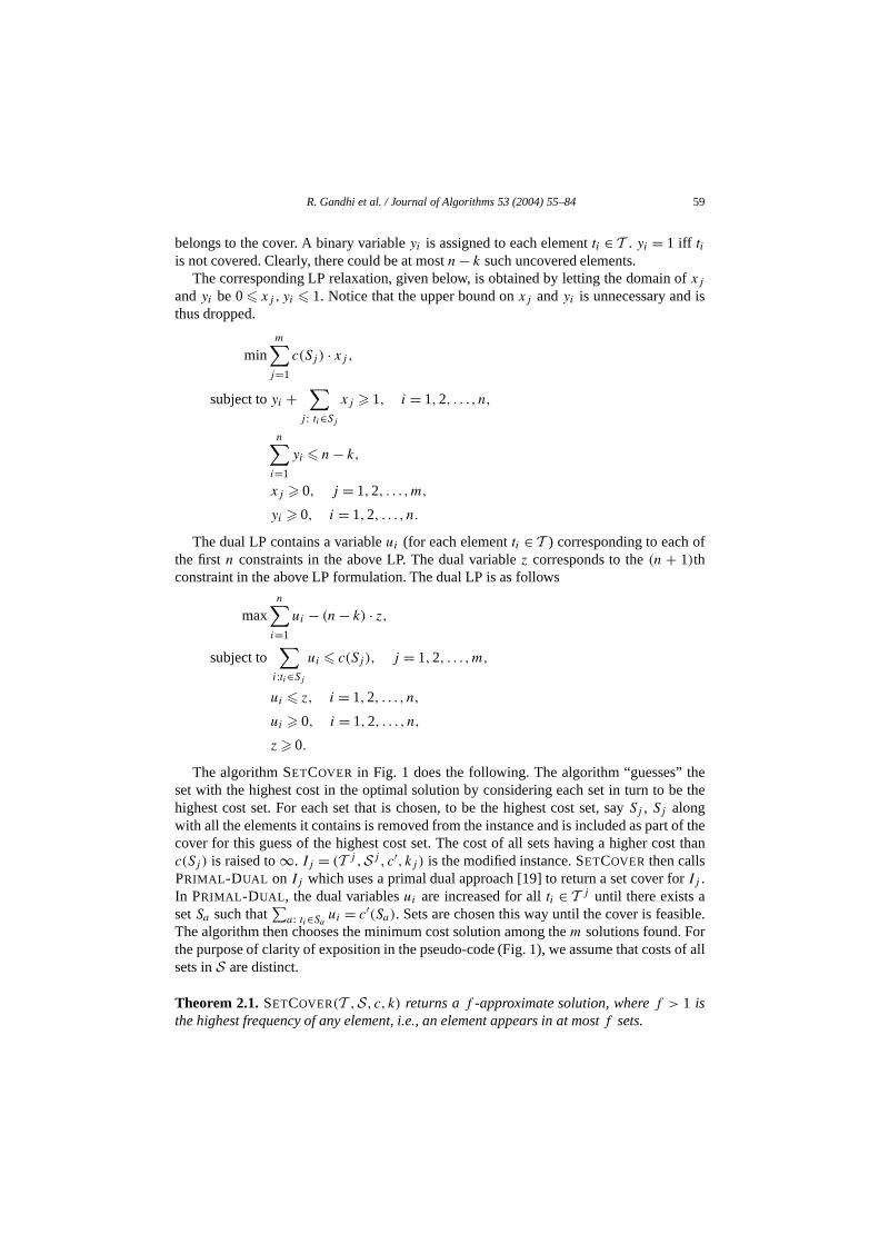
belongs to the cover. A binary variableyi is assigned to each elementti ∈ T . yi = 1 iff tiis not covered. Clearly, there could be at mostn − k such uncovered elements.

The corresponding LP relaxation, given below, is obtained by letting the domain ofxj

andyi be 0 xj , yi 1. Notice that the upper bound onxj andyi is unnecessary andthus dropped.

minm∑

j=1

c(Sj ) · xj ,

subject toyi +∑

j : ti∈Sj

xj 1, i = 1,2, . . . , n,

n∑i=1

yi n − k,

xj 0, j = 1,2, . . . ,m,

yi 0, i = 1,2, . . . , n.

The dual LP contains a variableui (for each elementti ∈ T ) corresponding to each othe firstn constraints in the above LP. The dual variablez corresponds to the(n + 1)thconstraint in the above LP formulation. The dual LP is as follows

maxn∑

i=1

ui − (n − k) · z,

subject to∑

i:ti∈Sj

ui c(Sj ), j = 1,2, . . . ,m,

ui z, i = 1,2, . . . , n,

ui 0, i = 1,2, . . . , n,

z 0.

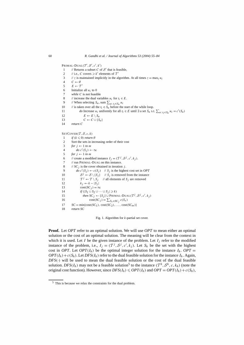
The algorithm SETCOVER in Fig. 1 does the following. The algorithm “guesses” tset with the highest cost in the optimal solution by considering each set in turn to be thighest cost set. For each set that is chosen, to be the highest cost set, saySj , Sj alongwith all the elements it contains is removedfrom the instance and is included as part ofcover for this guess of the highest cost set. The cost of all sets having a higher coc(Sj ) is raised to∞. Ij = (T j ,Sj , c′, kj ) is the modified instance. SETCOVER then callsPRIMAL -DUAL on Ij which uses a primal dual approach [19] to return a set cover foIj .In PRIMAL -DUAL , the dual variablesui are increased for allti ∈ T j until there exists asetSa such that

∑a: ti∈Sa

ui = c′(Sa). Sets are chosen this way until the cover is feasiThe algorithm then chooses the minimum cost solution among them solutions found. Fothe purpose of clarity of exposition in the pseudo-code (Fig. 1), we assume that costsets inS are distinct.

Theorem 2.1. SETCOVER(T ,S, c, k) returns af -approximate solution, wheref > 1 isthe highest frequency of any element, i.e., an element appears in at mostf sets.


lxt in

t

sible

PRIMAL -DUAL (T ′,S ′, c′, k′)1 // Returns a subsetC of S ′ that is feasible,2 // i.e.,C covers k′ elements ofT ′3 // z is maintained implicitly in the algorithm. At all timesz = maxi ui

4 C ← ∅5 E ← T ′6 Initialize allui to 07 while C is not feasible8 // increase the dual variablesui for ti ∈ E.9 // When selectingSa , sum

∑a: ti∈Sa

ui

10 // is taken over all theti ∈ Sa before the start of the while loop.11 do Increaseui uniformly for all ti ∈ E until ∃ a setSa s.t.

∑a: ti∈Sa

ui = c′(Sa)

12 E ← E \ Sa

13 C ← C ∪ Sa14 return C

SETCOVER(T ,S, c, k)

1 if (k 0) return ∅2 Sort the sets in increasing order of their cost3 for j ← 1 to m

4 do c′(Sj ) ← ∞5 for j ← 1 to m

6 // create a modified instanceIj = (T j ,Sj , c′, kj ).7 // run PRIMAL -DUAL on this instance.8 // SCj is the cover obtained in iterationj .9 do c′(Sj ) ← c(Sj ) // Sj is the highest cost set inOPT

10 Sj ← S \ Sj // Sj is removed from the instance11 T j ← T \ Sj // all elements ofSj are removed12 kj ← k − |Sj |13 cost(SCj ) = ∞14 if (|S1 ∪ S2 ∪ · · · ∪ Sj | k)

15 then SCj ← Sj ∪ PRIMAL -DUAL (T j ,Sj , c′, kj )

16 cost(SCj ) = ∑Sx∈SCj

c(Sx)

17 SC= mincost(SC1), cost(SC2), . . . , cost(SCm)18 return SC

Fig. 1. Algorithm fork-partial set cover.

Proof. Let OPT refer to an optimal solution. We will useOPT to mean either an optimasolution or the cost of an optimal solution. The meaning will be clear from the contewhich it is used. LetI be the given instance of the problem. LetIj refer to the modifiedinstance of the problem, i.e.,Ij = (T j ,Sj , c′, kj ). Let Sh be the set with the highescost in OPT. Let OPT(Ih) be the optimal integer solution for the instanceIh. OPT =OPT(Ih)+c(Sh). LetDFS(Ih) refer to the dual feasible solution for the instanceIh. Again,DFS(·) will be used to mean the dual feasible solution or the cost of the dual feasolution.DFS(Ih) may not be a feasible solution5 to the instance(T h,Sh, c, kh) (note theoriginal cost function). However, sinceDFS(Ih) OPT(Ih) andOPT= OPT(Ih)+c(Sh),

5 This is because we relax the constraints for the dual problem.


thetfthe

ee

n that

e

g oneslved in

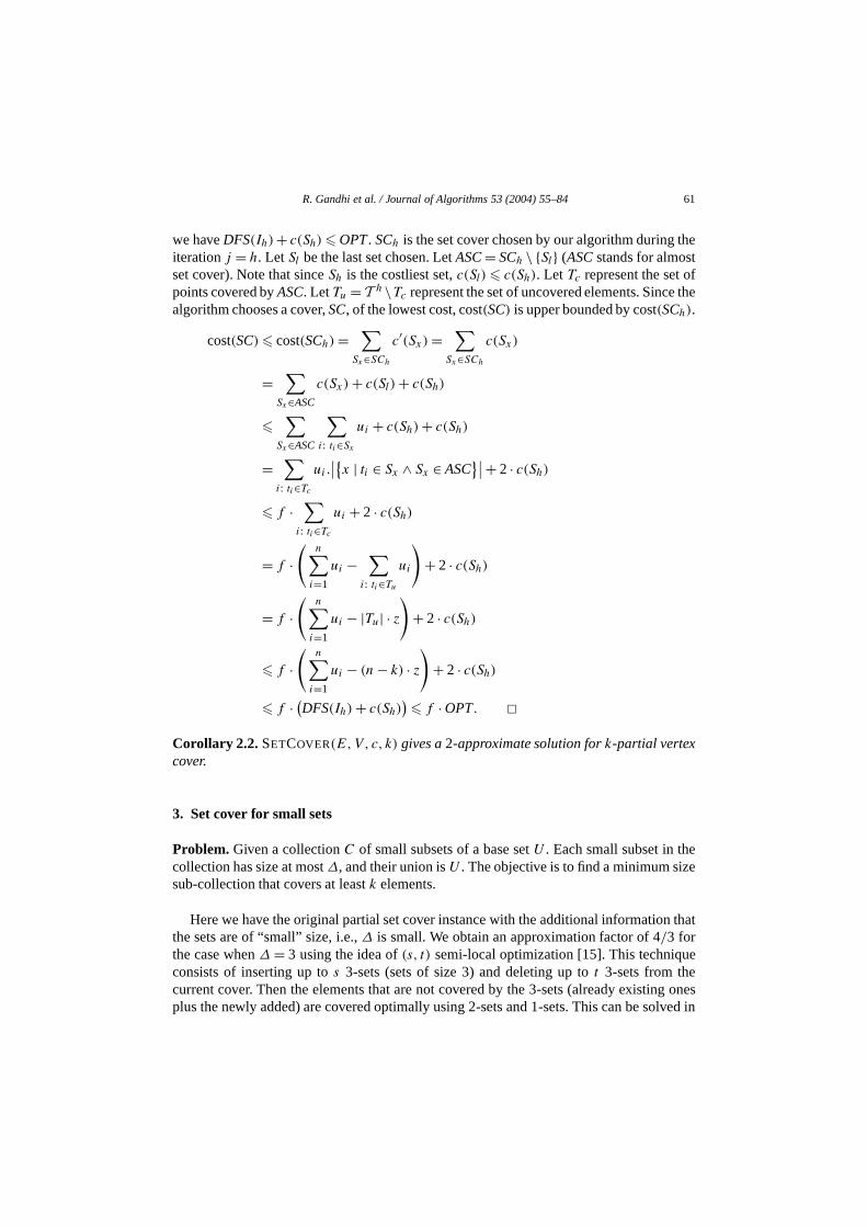
we haveDFS(Ih) + c(Sh) OPT. SCh is the set cover chosen by our algorithm duringiterationj = h. Let Sl be the last set chosen. LetASC= SCh \ Sl (ASCstands for almosset cover). Note that sinceSh is the costliest set,c(Sl) c(Sh). Let Tc represent the set opoints covered byASC. LetTu = T h \Tc represent the set of uncovered elements. Sincealgorithm chooses a cover,SC, of the lowest cost, cost(SC) is upper bounded by cost(SCh).

cost(SC) cost(SCh) =∑

Sx∈SCh

c′(Sx) =∑

Sx∈SCh

c(Sx)

=∑

Sx∈ASC

c(Sx) + c(Sl) + c(Sh)

∑

Sx∈ASC

∑i: ti∈Sx

ui + c(Sh) + c(Sh)

=∑

i: ti∈Tc

ui.∣∣x | ti ∈ Sx ∧ Sx ∈ ASC

∣∣ + 2 · c(Sh)

f ·∑

i: ti∈Tc

ui + 2 · c(Sh)

= f ·(

n∑i=1

ui −∑

i: ti∈Tu

ui

)+ 2 · c(Sh)

= f ·(

n∑i=1

ui − |Tu| · z)

+ 2 · c(Sh)

f ·(

n∑i=1

ui − (n − k) · z)

+ 2 · c(Sh)

f · (DFS(Ih) + c(Sh)) f · OPT.

Corollary 2.2. SETCOVER(E,V, c, k) gives a2-approximate solution fork-partial vertexcover.

3. Set cover for small sets

Problem. Given a collectionC of small subsets of a base setU . Each small subset in thcollection has size at most∆, and their union isU . The objective is to find a minimum sizsub-collection that covers at leastk elements.

Here we have the original partial set cover instance with the additional informatiothe sets are of “small” size, i.e.,∆ is small. We obtain an approximation factor of 4/3 forthe case when∆ = 3 using the idea of(s, t) semi-local optimization [15]. This techniquconsists of inserting up tos 3-sets (sets of size 3) and deleting up tot 3-sets from thecurrent cover. Then the elements that are not covered by the 3-sets (already existinplus the newly added) are covered optimally using 2-sets and 1-sets. This can be so


mentsximumximumber

h fewere the oneof each

hoosee totalrm

ageh and

s in theks

lutionetste

eyber of

case,

nd on

or

e

or

polynomial time using maximum matching [17]. The vertices are the uncovered eleof U and the edges are the admissible 2-sets. The 2-sets corresponding to the mamatching edges and the 1-sets corresponding to the vertices not covered by the mamatching form an optimum covering. We will order the quality of a solution by the numof sets in the cover and among two covers of the same size we choose the one wit1-sets and if the covers have the same size and neither cover has a 1-set we choosthat covers more elements. Without loss of generality, we assume that all subsetsset are available and hence all coverings are assumed to be disjoint.

The algorithm starts with any solution. One solution can be obtained as follows. Ca maximal collection of disjoint 3-sets. Cover the remaining elements (such that thnumber of elements covered are at leastk) optimally using 2-sets and 1-sets. Perfosemi-local(2,1) improvements until no improvement is possible.

The proof for the bound of 4/3 for full coverage does not extend to the partial coverversion. For the full coverage, to prove the lower bound on the optimal solution DuFürer [15] construct a graphG in which the vertices are the sets chosen byOPT and theedges are 1-sets and 2-sets of the approximate solution. They prove thatG cannot havemore than one cycle and hence argue that the total number of 1-sets and 2-setsolution is a lower bound onOPT. This works well for the full coverage version but breadown for the partial covering problem. For the partial covering case,G having at most onecycle is a necessary but not a sufficient condition to prove the lower bound.

In the full coverage version of the problem, to bound the number of 1-sets in the sothey construct a bipartite graph with the twosets of vertices corresponding to the schosen by the approximate solution andOPT. If a set corresponding to the approximasolution intersects a set corresponding toOPT in m elements then there arem edgesbetween their corresponding vertices in the graph. In each component of the graph thshow that the number of 1-sets of the solution in that component is at most the num1-sets ofOPT in that component. This is clearly not the case in the partial coveringsince our solution may have a 1-set that covers an element thatOPT may not cover. Weobtain a bound on the number of 1-sets as a side effect of the proof for the lower bouOPT.

3.1. Analysis

Notation.

S: our solution.OPT: optimal solution.

ai : number of sets of sizei (i = 1,2,3) in S.bi : number of sets of sizei (i = 1,2,3) in OPT.B: set of elements covered by 2-sets or 3-sets ofS and neither covered by 2-sets n

3-sets ofOPT, i.e.,B represents “bad” elements.C: set of elements covered by 2-sets or 3-sets ofS and OPT, i.e., C represents th

elements common toS andOPT.D: set of elements covered by 2-sets or 3-sets ofOPT and neither covered by 2-sets n

3-sets ofS, i.e.,D represents desirable elements.


r this

toly.e used

it is

p).aeis

ummy

nentofioni-localthese

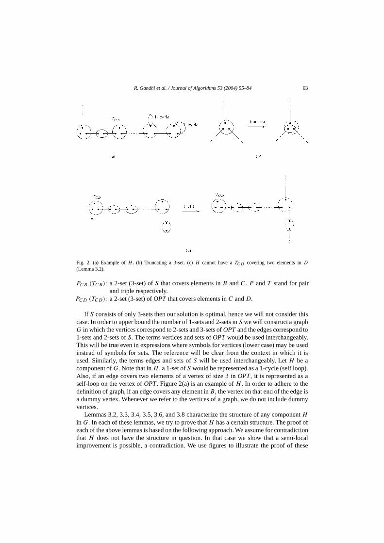
Fig. 2. (a) Example ofH . (b) Truncating a 3-set. (c)H cannot have aTCD covering two elements inD(Lemma 3.2).

PCB (TCB): a 2-set (3-set) ofS that covers elements inB andC. P andT stand for pairand triple respectively.

PCD (TCD): a 2-set (3-set) ofOPT that covers elements inC andD.

If S consists of only 3-sets then our solution is optimal, hence we will not considecase. In order to upper bound the number of 1-sets and 2-sets inS we will construct a graphG in which the vertices correspond to 2-sets and 3-sets ofOPTand the edges correspond1-sets and 2-sets ofS. The terms vertices and sets ofOPT would be used interchangeabThis will be true even in expressions where symbols for vertices (lower case) may binstead of symbols for sets. The reference will be clear from the context in whichused. Similarly, the terms edges and sets ofS will be used interchangeably. LetH be acomponent ofG. Note that inH , a 1-set ofS would be represented as a 1-cycle (self looAlso, if an edge covers two elements of a vertex of size 3 inOPT, it is represented asself-loop on the vertex ofOPT. Figure 2(a) is an example ofH . In order to adhere to thdefinition of graph, if an edge covers any element inB, the vertex on that end of the edgea dummy vertex. Whenever we refer to the vertices of a graph, we do not include dvertices.

Lemmas 3.2, 3.3, 3.4, 3.5, 3.6, and 3.8 characterize the structure of any compoH

in G. In each of these lemmas, we try to prove thatH has a certain structure. The proofeach of the above lemmas is based on the following approach. We assume for contradictthat H does not have the structure in question. In that case we show that a semimprovement is possible, a contradiction. We use figures to illustrate the proof of


ise andsts oft.ies

the

tsts

us,

ch

aboveur

.ding2-setsd.

e

ver

lustrates

then

lemmas. In each of the figures, we will show the result when semi-local improvementapplied toH . The scenario before the improvement is shown on the left of each figuron the right we show the improved partial cover. The improved partial cover consisome sets that were part ofOPT and some sets that were part ofS before the improvemenIn the improved solution the sets ofOPT that we include are marked by solid boundarand the sets ofS that we include are represented by solid edges.

We will now introduce some notation that will be used heavily in the proofs oflemmas. Foranyvertexz in G, let zt denote truncatedz. We definezt as follows. Ifz isa 2-set thezt = z, otherwisezt covers exactly two of the three elements ofz. Figure 2(b)shows a 3-set that is truncated. LetP be a path inH between verticesu andw. Let Ip andEp denote the set ofinternalvertices and set of edges inP respectively. Thus,Ip containsall vertices ofP other thanu andw. Hence,|Ip| = |Ep| − 1. LetFp denote the elemencovered by edges inEp . Also, every 3-set,t , in Ip is truncated to contain the two elemenin t ∩ Fp . ThusIp consists of only 2-sets. Ifu or w is aTCD , sayu, thenut consists ofan element inD and the element inu ∩ Ep . For any cycleC in H , let Vc andEc denotethe vertices and edges respectively ofC. For any vertexw ∈ C, let Icw = Vc \ w, whereagain the 3-sets are truncated to contain itselements that are covered by the cycle. ThIcw consists of only 2-sets. Note that∀w ∈ Vc, |Icw| = |Ec| − 1.

Lemma 3.1. The semi-local(2,1)-optimization algorithm produces a solution in whia1 + 2a2 + 3a3 b1 + 2b2 + 3b3 + 1.

Proof. Note thatk b1 + 2b2 + 3b3. If a1 > 0 thenS covers exactlyk elements. Ifa1 = 0then it may cover an extra element and hence the 1 on the right hand side of theinequality. Recall that ifa1 = 0, thena2 > 0 since we cannot have only 3-sets in osolution.

Recall thatS and OPT represent our solution and an optimal solution respectivelyW.l.o.g. we can modifyS as follows. When we compute an optimal solution corresponto a certain choice of 3-sets, we pick a solution that maximizes the number ofbelonging toOPT. This does not affect the size ofS or the number of elements covereThe following lemmas apply to the graphH corresponding to the modifiedS.

Lemma 3.2. If H has aTCD that covers two elements inD then the third element must bshared with a3-set ofS. If H has a triple with three elements inD then our solution isoptimal.

Proof. Consider the case whenH has a triplew that covers exactly two elements inDand the third element is shared with a 1-set or a 2-set ofS. We will show that a(1,0)

optimization (insertingw) gives an improved solution, a contradiction. The new cowould beS ∪ w \ ew, whereew is the edge incident onw in H . The new solutioncovers more elements and uses the same number of sets as before. Figure 2(c) ilthis case. Now consider the case whenw is a triple that covers three elements inD. In thiscase, our solution must contain all triples, i.e., our solution must be optimal. If not,


nt

by

n by

er the

scover

of each

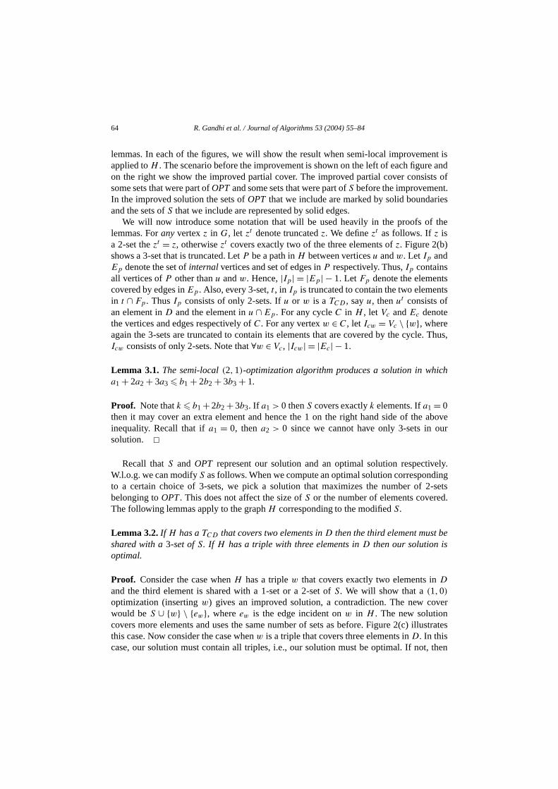
we can cover at least one extra element using the same number of sets by swappingw withsome 2-set or 1-set inS. This is equivalent to a(1,0) semi-local improvement. Lemma 3.3. H has at most one set of OPT that covers elements inC andD.

Proof. Assume otherwise. Consider a pathP in H between two verticesw1 andw2 thatcover elements inC andD. By Lemma 3.2,w1 andw2 each cover exactly one elemein D. Let ei /∈ Ep represent an edge inH that is incident onwi . This happens only ifwi

is aTCD. We will consider the following three cases based on the sets representedw1andw2.

Case I. w1 = TCD andw2 = TCD.

We will contradict our assumption by showing that we can obtain a better solutioperforming a(2,0) semi-local optimization (insertingw1 andw2). Let the new cover be(S ∪ Ip ∪ w1,w2) \ (Ep ∪ e1, e2). The size of the new cover is(|S| + |Ep| − 1+ 2) −(|Ep| + 2) = |S| − 1. The new solution covers all the elements inFp . Moreover, the newsolution covers 2 extra elements due tow1 andw2 and loses 2 elements due toe1 ande2.All other edges ofS are included in the new solution. Thus we use one less set to covsame number of elements. Figure 3(a) illustrates this case.

Case II. w1 = TCD andw2 = PCD .

We will show how to obtain a better solution by performing a(1,0) semi-localoptimization (insertingw1), a contradiction. Let the new cover be(S ∪ Ip ∪ w1,w2) \(Ep ∪e1). The size of the new cover is(|S|+ |Ep|−1+2)− (|Ep|+1) = |S|. We coveran extra element since we cover 2 extra elements due tow1 andw2 and lose 1 elementdue toe1. Thus we have an improved solution that uses the same number of sets tomore elements. This case is illustrated in Fig. 3(b).

Case III. w1 = PCD andw2 = PCD .

This cannot happen asS maximizes the number of 2-sets belonging toOPT. Figure 3(c)illustrates this case. This is an example where we use the assumption that all subsetsset are available. Lemma 3.4. If H has aTCD or PCD thenH is acyclic.

Proof. Assume otherwise. Letw denote the set ofOPT that covers elements inC andD.Let u be the vertex of the cycle,L, that is closest tow. Consider the pathP betweenw andu. Note that by Lemma 3.3,u cannot be aTCD or a PCD . We will consider thefollowing cases.

Case I. w = TCD or PCD andu is a 3-set.


figuresd

a

es

notent.hence it

Fig. 3. Examples for Lemma 3.3. In each of the following cases an improved partial cover (represented byon the right) contains the sets ofOPT marked by solid boundaries and the sets ofS corresponding to the soliedges. (a) TwoTCD sets inH lead to a(2,0) semi-local improvement. (b) ATCD and PCD in H leads toa (1,0) semi-local improvement. (c) TwoPCD sets inOPT is not possible as, w.l.o.g., our algorithm findssolution maximizing the number of 2-sets belonging toOPT.

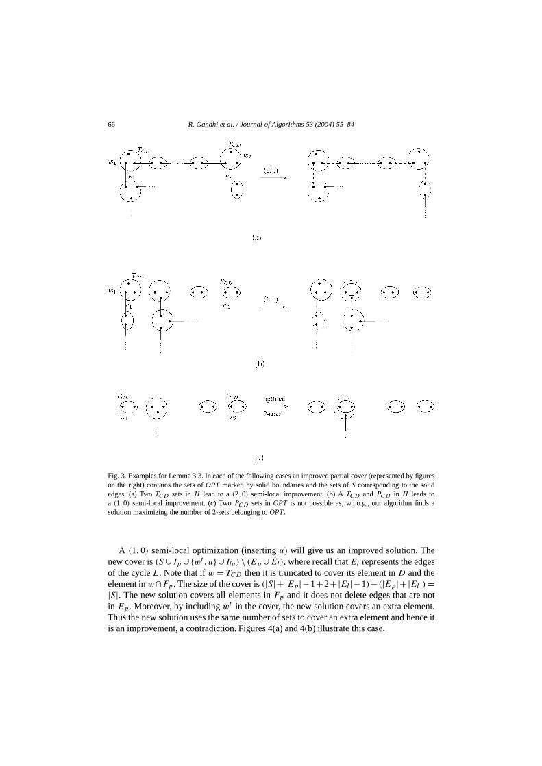
A (1,0) semi-local optimization (insertingu) will give us an improved solution. Thnew cover is(S ∪ Ip ∪ wt ,u ∪ Ilu) \ (Ep ∪El), where recall thatEl represents the edgeof the cycleL. Note that ifw = TCD then it is truncated tocover its element inD and theelement inw∩Fp . The size of the cover is(|S|+|Ep|−1+2+|El |−1)−(|Ep|+|El |) =|S|. The new solution covers all elements inFp and it does not delete edges that arein Ep. Moreover, by includingwt in the cover, the new solution covers an extra elemThus the new solution uses the same number of sets to cover an extra element andis an improvement, a contradiction. Figures 4(a) and 4(b) illustrate this case.


figuresdan

ppen

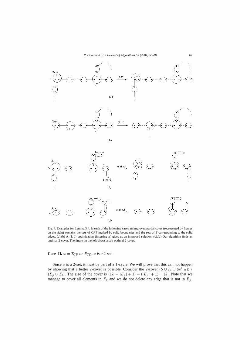
Fig. 4. Examples for Lemma 3.4. In each of the following cases an improved partial cover (represented byon the right) contains the sets ofOPT marked by solid boundaries and the sets ofS corresponding to the soliedges. (a),(b) A(1,0) optimization (insertingu) gives us an improved solution. (c),(d) Our algorithm findsoptimal 2-cover. The figure on the left shows a sub-optimal 2-cover.

Case II. w = TCD or PCD , u is a 2-set.

Sinceu is a 2-set, it must be part of a 1-cycle. We will prove that this can not haby showing that a better 2-cover is possible. Consider the 2-cover(S ∪ Ip ∪ wt,u) \(Ep ∪ El). The size of the cover is(|S| + |Ep| + 1) − (|Ep| + 1) = |S|. Note that wemanage to cover all elements inFp and we do not delete any edge that is not inEp .


,ment, a

edn

.

t

re 5(a)tin

)uldis

s

ich

boveare

Moreover, the new solution covers an extra element by includingwt in our cover. Thuswe get an improved 2-cover that uses the same number of sets to cover an extra elecontradiction. Figures 4(c) and 4(d) illustrate this case.

Case III. w = u.

We will show that a(1,0) semi-local optimization (insertingw) gives an improvedsolution, a contradiction. The new cover will be(S ∪w ∪ Ilw) \ (El). The size of the newcover is(|S| + 1+ |El| − 1) − |El| = |S|. In addition to covering all the elements coverby the cycle, the new solution covers an extra element due tow. Hence the new solutiouses the same number of sets to cover more elements.Lemma 3.5. H does not have more than one cycle.

Proof. By Lemma 3.4, the claim is true whenH has aTCD or aPCD, sinceH is acyclic.For the rest of the proof we will assume thatH does not contain aTCD or aPCD . Assumefor contradiction thatH has two cyclesC1 andC2. We will consider the following cases

Case I. C1 andC2 are disjoint.

Let u ∈ C1 and w ∈ C2 be the closest pair of vertices on the two cycles and leP

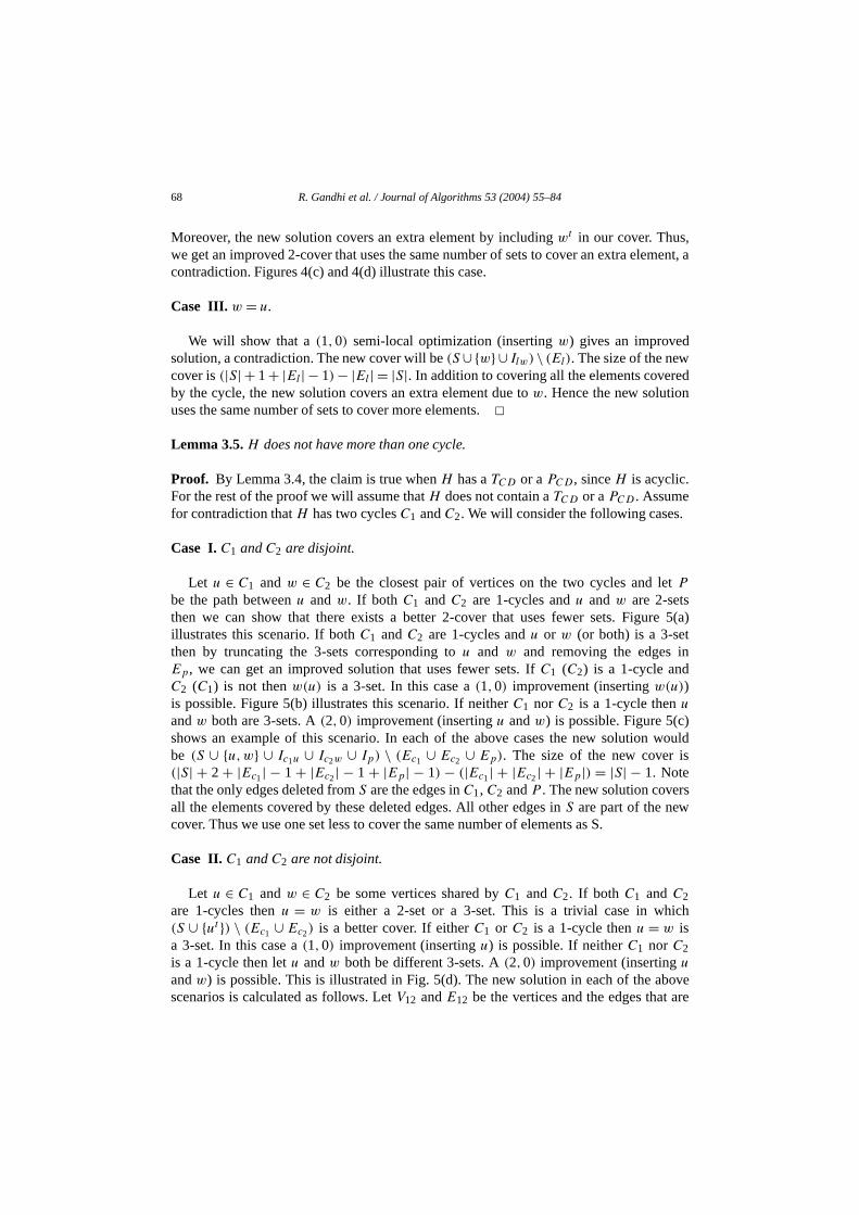
be the path betweenu and w. If both C1 and C2 are 1-cycles andu and w are 2-setsthen we can show that there exists a better 2-cover that uses fewer sets. Figuillustrates this scenario. If bothC1 andC2 are 1-cycles andu or w (or both) is a 3-sethen by truncating the 3-sets corresponding tou and w and removing the edgesEp, we can get an improved solution that uses fewer sets. IfC1 (C2) is a 1-cycle andC2 (C1) is not thenw(u) is a 3-set. In this case a(1,0) improvement (insertingw(u))is possible. Figure 5(b) illustrates this scenario. If neitherC1 nor C2 is a 1-cycle thenuandw both are 3-sets. A(2,0) improvement (insertingu andw) is possible. Figure 5(cshows an example of this scenario. In eachof the above cases the new solution wobe (S ∪ u,w ∪ Ic1u ∪ Ic2w ∪ Ip) \ (Ec1 ∪ Ec2 ∪ Ep). The size of the new cover(|S| + 2 + |Ec1| − 1 + |Ec2| − 1 + |Ep| − 1) − (|Ec1| + |Ec2| + |Ep|) = |S| − 1. Notethat the only edges deleted fromS are the edges inC1, C2 andP . The new solution coverall the elements covered by these deleted edges. All other edges inS are part of the newcover. Thus we use one set less to cover the same number of elements as S.

Case II. C1 andC2 are not disjoint.

Let u ∈ C1 and w ∈ C2 be some vertices shared byC1 and C2. If both C1 and C2are 1-cycles thenu = w is either a 2-set or a 3-set. This is a trivial case in wh(S ∪ ut ) \ (Ec1 ∪ Ec2) is a better cover. If eitherC1 or C2 is a 1-cycle thenu = w isa 3-set. In this case a(1,0) improvement (insertingu) is possible. If neitherC1 nor C2is a 1-cycle then letu andw both be different 3-sets. A(2,0) improvement (insertinguandw) is possible. This is illustrated in Fig. 5(d). The new solution in each of the ascenarios is calculated as follows. LetV12 andE12 be the vertices and the edges that


.

is

ber of

Fig. 5. Examples for Lemma 3.5. (a),(b),(c) Semi-local improvement in the case whenH has two disjoint cycles(d) A (2,0) improvement leads to a better solution when neitherC1 andC2 are not disjoint and neither of themare 1-cycles.

shared byC1 andC2. Let V1−2 andE1−2 be the vertices and edges that are inC1 and notin C2. Let V2−1 andE2−1 be the vertices and edges that are inC2 and not inC1. Notethat |V12| = |E12| + 1, |V1−2| = |E1−2| − 1 and|V2−1| = |E2−1| − 1. The new solutionwould be(S ∪ V1−2 ∪ V2−1 ∪ V12) \ (E1−2 ∪ E2−1 ∪ E12). The size of the new cover(|S| + |E1−2| − 1+ |E2−1| − 1+ |E12| + 1) − (|E1−2| + |E2−1| + |E12|) = |S| − 1. Againfollowing the same argument as in Case I, the new solution covers the same numelements asS, but using one set less.


d

neer the

.rts

the

ich

he

rged

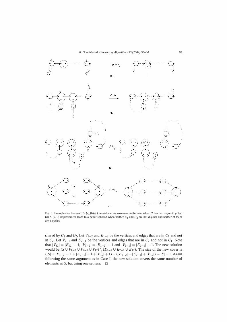
Fig. 6. Examples for Lemma 3.6. In the above instances(0,1) semi-local improvement yields an improvesolution.

Lemma 3.6. If a1 > 0 and ifH contains aTCD or PCD thenH does not have a2-set or a3-set of OPT that shares elements with a3-set ofS, i.e.,H does not have a2-set or a3-setof OPT sayx, such thatx ∩ y = ∅, wherey is a 3-set ofS.

Proof. Let r be a 1-set ofS. Let u denote aTCD or PCD in H . Consider the case wheu andx denote the same set. In that case a(0,1) semi-local improvement (removing th3-sety) will cover the same number of elements using fewer 1-sets. Now we considcase whenu andx denote different sets. Consider a pathP betweenu andx in H . In thiscase a(0,1) semi-local improvement (removing the 3-sety) is possible, a contradictionThe new solution would be(S ∪ xt , yt , ut ∪ Ip) \ (y ∪ Ep ∪ r). The size of the coveis (|S| + 3 + |Ep| − 1) − (1 + |Ep| + 1) = |S|. The new solution covers all the elemencovered byy ∪Ep . The new solution covers an element inD by insertingut . This accountsfor the element covered byr that is not in the new solution. Thus the new cover is ofsame size as the old one, however the new solution has one singleton less than inS. Henceit is an improved solution. Figure 6 illustrates some of the cases.

Lemma 3.7. The (2,1) semi-local optimization technique produces a solution in wha1 + a2 b1 + b2 + b3 + 1.

Proof. The outline of our proof is as follows. In each componentH we will charge theedges (sets ofS) to the vertices (sets ofOPT) of H . Our charging scheme satisfies tfollowing property. Each vertex is charged by at most one edge and an edgee is chargedto a vertexv only if |e ∩ B| |v ∩ D|. We then argue that each edge that is not cha


hat

tn

d

aent

le.eans

d

nt

r

er ofer

ave

to any vertex must cover an element inB. Through careful arguments we then show tthese edges can be accounted for by vertices inOPT that are not yet charged.

We will now introduce some notation that will be used in the proof of this claim. LeOc

be the vertices inOPT that are charged by some edge. LetOu be the remaining vertices iOPT. Let ou = |Ou| andoc = |Oc|. Let au

i , i ∈ 1,2, be the number of sets of sizei thatare not charged to any set inOPT. Let ac

i be the number of sets of sizei that are chargeto some set ofOPT.

Below are the details of the proof. Our proof considers the following two cases.

Case I. a1 > 0.

In this case,OPT cannot contain a set with two elements inD; otherwise, we can use2-set to cover the two elements inD and drop a singleton thereby covering an extra elemusing the same number of sets. In each componentH , we will charge an edgee to a vertexv using the charging scheme described below. LetHs be the subgraph ofH that consistsof all the vertices ofH and all edges ofH that do not cover any element inB. Considerthe following two cases.

Case I(a). All elements covered by the vertices ofH are inC.

By Lemma 3.5,H has at most one cycle. Thus,Hs is a tree or contains just one cycHence, inHs the number of vertices is at least equal to the number of edges. This mthat each edge inHs can be charged to a vertex inHs . The edges ofH that are not chargeto any vertex cover an element inB.

Case I(b). H consists of vertices that cover elements inD.

By Lemma 3.3,H has exactly one such vertex, sayw. By Lemma 3.4,H can not haveany cycles. In this case,Hs is a tree. We can charge all the edges inHs to all the verticesin Hs , exceptw. Thus all the edges inH that do not cover any element inB are chargedto some vertex inH . By Lemma 3.6, the number of edges incident on every vertex iH

exceptw must be equal to the size of the vertex. This means thatH must have at leasonePCB . We charge one suchPCB to w. As in the previous case, the edges ofH that arenot charged to any vertex must cover an element inB. Below we show how to account fothese edges.

Note thatau1 is the number of singleton sets ofS that cover an element inB. All other

1-sets ofS cover elements inC and hence are charged to some set ofOPT. We haveac

1 + ac2 = oc. Recall thatOPT cannot have a set with two elements inD. Also, since

a1 > 0, S and OPT cover exactly the same number of elements. Thus the numbuncharged vertices together with the singletons inOPTmust be at least equal to the numbof elements inB covered by the edges that are not charged to any vertex. Thus we h

au1 + au

2 b1,

au1 + au

2 + ac1 + ac

2 b1 + oc,

a1 + a2 b1 + b2 + b3. (1)


ts tohere is-

d to

etlrged

ayer

y

3-set

berhen the

er ofr

Case II. a1 = 0.

We analyze this case by again considering two cases.

Case II(a). H contains a3-setw that does not share elements with any3-set inS.

In this case there can be at most one set inOPT that covers two elements inD.Otherwise, a(1,0) improvement (insertingw) is possible as follows. By Lemma 3.2,w

cannot have two elements inD. If w is a TCD then we can swapw with the two edgesincident on it and use a 2-set to cover two elements inD. If all elements ofw are inC thenwe can includew in our cover along with two 2-sets to cover the four elements inD anddelete the three edges incident onw. In both the cases we use the same number of secover one extra element. For the remainder of the argument we will assume that tat most one set covering two elements inD. We denote this set byt . We analyze this subcase by using the same charging scheme as in Case I. As in Case I(a), whenH consists ofvertices that only cover elements inC, we can show that the edges that are not chargeany vertex contain an element inB. Now consider the case whenH has a vertex, sayd , thatcovers an element inD. In this case, one vertex ofH may not be charged by any edge. Lthis vertex bed . The vertexd may cover two elements inD and by our charging rule it wilnot be charged. Recall thatau

2 denotes the number of edges of size two that are not chato any vertex. Note that each edge that is not charged to any vertex covers an element inB.First, we will boundau

2 for the case whent does not exist. In this case our solution mcoverk + 1 elements. Hence,au

2 ou + b1 + 1. If t exists thenS covers the same numbof elements asOPT. If not, then a(1,0) improvement (insertingw) is possible. This isbecause ifw is aTCD then we can swapw for the two edges incident on it and ifw is nota TCD then we can includew andt and delete the three edges incident onw. In both thecases we use one set less to cover one less element. Also, note thatt is not charged by anedge and belongs to the setOu. Hence, we haveau

2 (ou + 1) + b1 = ou + b1 + 1. Thus,whethert exists or not the bound onau

2 is the same.

au2 ou + b1 + 1,

au2 + ac

2 ou + b1 + 1+ oc,

a2 b1 + b2 + b3 + 1,

a1 + a2 b1 + b2 + b3 + 1.

Case II(b). H does not containw.

In this case, ifH contains a vertex of size three then it shares an element with aof S. Hence, at most two elements of any vertex can be covered by edges inH . Hence,His either a cycle or a path. InH , if the number of edges is less than or equal to the numof vertices then each edge is charged to some vertex. Now consider the case wnumber of edges inH is greater than the number of vertices inH . In this case,H has twoelements inB and none inD. Since the number of edges is one more than the numbvertices, exactly one edge inH is not charged to any vertex inH . Observe that the numbe


ize

red by

n

t

ofn.

ich

.

sBy

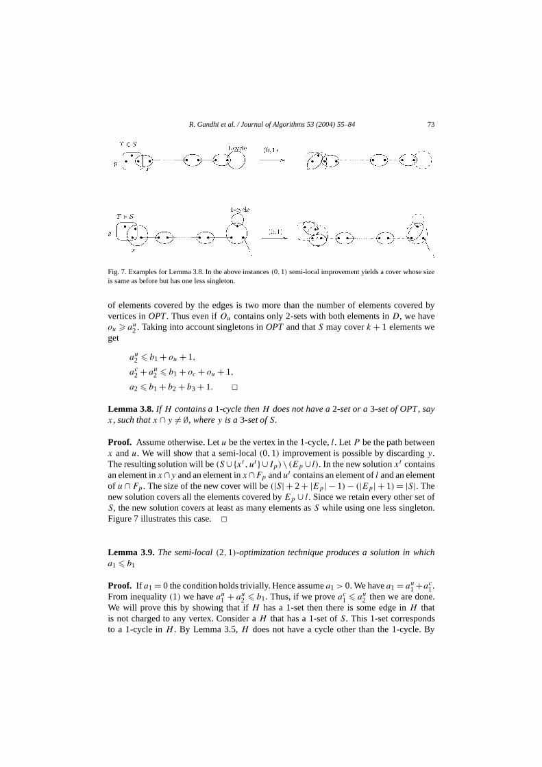
Fig. 7. Examples for Lemma 3.8. In the above instances(0,1) semi-local improvement yields a cover whose sis same as before but has one less singleton.

of elements covered by the edges is two more than the number of elements covevertices inOPT. Thus even ifOu contains only 2-sets with both elements inD, we haveou au

2. Taking into account singletons inOPT and thatS may coverk + 1 elements weget

au2 b1 + ou + 1,

ac2 + au

2 b1 + oc + ou + 1,

a2 b1 + b2 + b3 + 1. Lemma 3.8. If H contains a1-cycle thenH does not have a2-set or a3-set of OPT, sayx, such thatx ∩ y = ∅, wherey is a 3-set ofS.

Proof. Assume otherwise. Letu be the vertex in the 1-cycle,l. Let P be the path betweex andu. We will show that a semi-local(0,1) improvement is possible by discardingy.The resulting solution will be(S ∪xt , ut ∪ Ip)\ (Ep ∪ l). In the new solutionxt containsan element inx ∩y and an element inx ∩Fp andut contains an element ofl and an elemenof u ∩ Fp . The size of the new cover will be(|S| + 2+ |Ep| − 1) − (|Ep| + 1) = |S|. Thenew solution covers all the elements covered byEp ∪ l. Since we retain every other setS, the new solution covers at least as many elements asS while using one less singletoFigure 7 illustrates this case.

Lemma 3.9. The semi-local(2,1)-optimization technique produces a solution in wha1 b1

Proof. If a1 = 0 the condition holds trivially. Hence assumea1 > 0. We havea1 = au1 +ac

1.From inequality(1) we haveau

1 + au2 b1. Thus, if we proveac

1 au2 then we are done

We will prove this by showing that ifH has a 1-set then there is some edge inH thatis not charged to any vertex. Consider aH that has a 1-set ofS. This 1-set correspondto a 1-cycle inH . By Lemma 3.5,H does not have a cycle other than the 1-cycle.


vele

ion ofproxi-anderandprove

n

ch

lved

e

Lemma 3.4,H does not have aTCD or PCD , i.e., all elements covered by the vertices ofH

are inC. By Lemma 3.8, there can not be a 3-set,y, of S such thatx ∩ y = ∅, wherex isa set ofOPT in H . Hence,H must have aPCB , saye. Consider the subgraph ofH , Hs asconstructed in Lemma 3.7.Hs contains all the vertices ofH and contains edges that haboth its endpoints inC. Thus,e is not part ofHs . SinceH has a 1-cycle,Hs has an equanumber of vertices and edges. Each vertex inHs and henceH get charged by some edgin Hs . Hence, edgee does not get charged to any vertex. This completes the proof.Theorem 3.10. The semi-local(2,1)-optimization algorithm for the3-set partial coveringproblem produces a solution that is within43OPT+ 1.

Proof. Adding up the inequalities in Lemmas 3.1, 3.7 and 3.9, we get

3(a1 + a2 + a3) 4(b1 + b2 + b3) − b1 − b2 + 2,

c(S) = a1 + a2 + a3 4

3OPT+ 2

3.

4. Probabilistic approaches for partial vertex cover

We now present a randomized rounding approach to the natural LP relaxatk-partial vertex cover. Analyzed in three different ways, this leads to three new apmation results mentioned in Section 1: relating to vertex cover (full coverage) for expgraphs of constant average degree,k-partial vertex cover on bounded-degree graphs,multi-criteriak-partial vertex cover problems. We first describe the basic method andsome probabilistic properties thereof, and then consider the three applications.

The k-partial vertex cover problem on a graphG = (V ,E) can be formulated as ainteger program as follows. We assign binary variablesxj for eachvj ∈ V andzi,j foreach(i, j) ∈ E. In this formulation,xj = 1 iff vertexvj belongs to the cover, andzi,j = 1iff edge(i, j) is covered. The corresponding LP relaxation can be obtained by letting eaxj andzi,j lie in [0,1].

minn∑

j=1

xj ,

subject toxi + xj zi,j , (i, j) ∈ E, (2)∑(i,j)∈E

zi,j k, (3)

xj , zi,j ∈ [0,1], ∀i, j.

Our basic approximation recipe will be as follows. The LP relaxation is sooptimally. Let x∗

i , z∗i,j denote an optimal LP solution, and letλ = 2(1 − ε), where

ε ∈ [0,1] is a parameter that will be chosen based on the application. LetS1 = vj | x∗j

1/λ, andS2 = V − S1. Include all the vertices inS1 as part of our cover, and mark thedges incident on vertices inS1 as covered. Now independently for eachj ∈ S2, roundxj to 1 with a probability ofλx∗, and to 0 with a probability of 1− λx∗. Let W be the
j j


r each

et Prl

ur

omin

of

ar

random variable denoting the number of covered edges at this point. IfW < k, we chooseanyk −W uncovered edges and cover them by arbitrarily choosing one end-point foof them.

We now introduce some notation to analyze the above process. Throughout, we l[·]and E[·] denote probability and expectation, respectively. Lety∗ represent the optimaobjective function value of the LP, and defineS0 ⊆ S1 by S0 = vj : x∗

j = 1. Let y∗F and

y∗P be the contribution toy∗ of the vertices inS0 andV − S0 respectively. Denote byUi,j

the event that edge(i, j) is uncovered. LetC1 be the cost of the solution produced by orandomized schemebeforethe step of coveringk −W edges if necessary, and letC2 be thecost incurred in covering thesek − W edges, if any. The total costC is of courseC1 + C2;thus,E[C] = E[C1] + E[C2]. Now, it is easy to check thatE[C1] y∗

F + λy∗P , and that

E[C2] E[maxk − W,0]. So we have

E[C] y∗F + λy∗

P + E[maxk − W,0]. (4)

The following lemma on the statistics ofW will be useful. As usual, letE denote thecomplement of an eventE .

Lemma 4.1.

(i) E[W ] k(1− ε2).(ii) Suppose the graphG has maximum degreed . Then, the varianceVar[W ] of W is at

most(2d − 1) · E[W ].

Proof. (i) Consider any edge(i, j). Now if x∗i 1/λ or x∗

j 1/λ, Pr[Ui,j ] = 0; otherwise,Pr[Ui,j ] = (1−λx∗

i )(1−λx∗j ). Consider the latter case. Sincex∗

i +x∗j z∗

i,j , we can checkthat for any givenz∗

i,j ∈ [0,1], (1 − λx∗i )(1 − λx∗

j ) is maximized whenx∗i = x∗

j = z∗i,j /2.

Hence,

Pr[Ui,j ] (1− λz∗

i,j /2)2 = (

1− (1− ε)z∗i,j

)2 1− z∗i,j

(1− ε2).

Thus, sinceE[W ] = ∑(i,j)∈E Pr[Ui,j ], we get

E[W ] ∑

(i,j)∈E

z∗i,j

(1− ε2) k

(1− ε2).

(ii) We haveW = ∑(i,j)∈E Ui,j . It is also an easy calculation to see that if a rand

variableW ′ is the sum ofpairwise independentrandom variables each of which lies[0,1], then Var[W ′] E[W ′]. However, the termsUi,j that constituteW do have somedependent pairs: if edges(i, j) and (i ′, j ′) share an endpoint, thenUi,j and Ui′,j ′ aredependent (positively correlated). Defineγ to be the sum, over all unordered pairsdistinct edges(i, j) and (i ′, j ′) that share an end-point, of Pr[Ui,j ∧ Ui′,j ′ ]. Using theabove observations and the definition of variance, a moment’s reflection shows that V[W ]is upper-bounded byE[W ] + 2γ . Now, for any eventsA andB,

Pr[A ∧ B] minPr[A],Pr[B]

(Pr[A] + Pr[B])/2.


t

averageber

reedy

rty is

4.2

,

Thus, the term “Pr[Ui,j ∧ Ui′,j ′ ]” in γ is at most(Pr[Ui,j ] + Pr[Ui′,j ′ ])/2. Finally, sinceeach edge has at most 2(d − 1) other edges that share an end-point with it, we get tha

γ ∑

(i,j)∈E

(2(d − 1)/2

) · Pr[Ui,j

] = (d − 1)E[W ].

So, Var[W ] E[W ] + 2γ (2d − 1) · E[W ]. 4.1. Vertex cover on expanders

Suppose we have a vertex cover problem; i.e.,k-partial vertex cover withk = m. TheLP relaxation here has “1” in place of “zi,j ” in (2), and does not require the variableszi,j

and the constraint (3). We focus here on the case of expander graphs of constantdegree. That is, for some constantsc andd , we are studying graphs where: (i) the numof edgesm is at mostnd , and (ii) for any setX of vertices with|X| n/2, at leastc|X|vertices outsideX have a neighbor inX.

Sincek = m, it is well-known that we can efficiently compute an optimal solutionx∗to the LP with all entries lying in0,1/2,1. Let H = vj | x∗

j = 1/2 and F = vj |x∗j = 1. Also, sinceW k = m always holds,E[maxk − W,0] = E[k − W ] mε2, by

Lemma 4.1(i). Thus, (4) shows thatE[C] is at mosty∗F + 2(1 − ε)y∗

H + mε2; followingthe notation underlying (4),y∗

H is the total contribution toy∗ from the vertices inH .(The overall approach of: (i) conducting a randomized rounding and then doing a gfixing of violated constraints, and (ii) using an equality such as our “E[maxk − W,0] =E[k − W ]” here, is suggested in [34]. We next show how the expansion propeuseful in boundingE[C] well. However, in the context ofpartial covering, an equalitysuch as “E[maxk − W,0] = E[k − W ]” does not hold; so, as discussed in Sectionsand 4.3, new analysis approaches are employed there.) Choosingε = y∗

H/m to minimizey∗F + 2(1− ε)y∗

H + mε2, we get

E[C] y∗H

(2− y∗

H/m) + y∗

F . (5)

Case I. |H | n/2.

Note that edges with exactly one end-point inH must have their other end-point inF ;otherwise the LP constraint on such edges will be violated. SinceG is an expander|F | c · |H |. Also, y∗

F = |F | and y∗H = |H |/2. So, sincey∗ = y∗

H + y∗F , we have

y∗H = y∗/(1+ a) for somea 2c. We can now use (5) to get

E[C] 2y∗H + y∗

F = (2− a/(1+ a)

)y∗;

i.e., at most(2− 2c/(1+ 2c))y∗ sincea 2c.

Case II. |H | > n/2.

So, we havey∗H n/4. Bound (5) shows thatE[C] (2− y∗

H/m)y∗; we havem nd

by assumption. So,E[C] (2− 1/(4d))y∗ in this case.


imation

m

mostell

sn-

, e.g.,

ng ofr thegiven

ethodtyver,

oris

hile, and

eastlts of

y

Thus we see thatE[C] [2 − min2c/(1 + 2c),1/(4d)] · y∗. In other words, for thefamily of expanders of constant average degree, we can get a constant-factor approxthat is strictly better than 2.

4.2. Partial vertex cover: bounded-degree graphs

We now show that for any constantd , k-partial vertex cover on graphs of maximudegree at mostd can be approximated to within 2(1 − Ω(1/d)), for any value ofthe parameterk. We also demonstrate that the integrality gap in this case is at2(1 − Ω(1/d)). We start with a couple of tail bounds that will be of use now, as was in Section 4.3. First, supposeX is a sum of independent random variablesXi eachof which lies in[0,1]; let E[X] = µ. Then for anyδ ∈ [0,1], the Chernoff bound showthat Pr[X µ(1 + δ)] is at moste−µδ2/3. We will also need tail bounds for certain noindependent situations. SupposeX is a random variable with meanµ and varianceσ 2;supposea > 0. Then, the well-known Chebyshev’s inequality states that Pr[|X − µ| a]is at mostσ 2/a2. We will need stronger tail bounds than this, but only onX’s one-sideddeviations (say, below its mean). We will use the Chebyshev–Cantelli inequality (see[1]), which shows that Pr[X − µ −a] σ 2/(σ 2 + a2).

We now analyze the performance of our basic algorithm (of randomized roundithe LP solution followed by a simple covering of a sufficient number of edges), fok-partial vertex cover problem on graphs with maximum degree bounded by someconstantd . The notation remains the same. The main problem in adopting the mof Section 4.1 here is as follows. Sincek equaledm there, we could use the equaliE[maxk −W,0] = E[k −W ], thus substantially simplifying the analysis. Here, howesuch an equality is not true; furthermore,E[maxX,Y ] maxE[X],E[Y ] for any pairof random variablesX,Y . (In fact, the two sides of this inequality may differ a lot. Finstance, supposeX is the sum ofn independent random variables, each of whichuniformly distributed on−1,1; let Y be the constant 0. Then the r.h.s. is zero, wthe l.h.s. isΘ(

√n).) Instead, we take recourse to the Chebyshev–Cantelli inequality

use Lemma 4.1(ii).We now claim that

Pr[W

(k(1− ε2) − 2

√kd

) ] 1/3. (6)

This is trivially true if k < 4d , since Pr[W 0] = 1. So supposek 4d . Lemma 4.1 andthe Chebyshev–Cantelli inequality show thatµ

.= E[W ] k(1 − ε2), and that Pr[W µ− 2

√dµ] 1/3. Subject toµ k(1− ε2) 4d(1− ε2), µ− 2

√dµ is minimized when

µ = k(1− ε2). Thus we have (6).Next, for a suitably large constantc0, we can assume thatk c0d

5. (Any optimalsolution has size at mostk, since in an optimal solution, every vertex should cover at lone new edge. So ifk is bounded by a constant—such asc0d

5—then we can find an optimasolution in polynomial time by exhaustive search.) Also, by adding all the constrainthe LP and simplifying, we get thaty∗ k/d . Let δ = 1/(3d). Assuming

ε 0.7, say, (7)

a Chernoff bound shows that immediately after the randomized rounding, the probabilitof having more than 2y∗(1 − ε)(1 + δ) vertices in our initial cover is at most 1/5


t

out

lvedion

ry

e.

dctivesible.

on

lity

s

(if the constantc0 is chosen large enough). Recall (6). So, with probability at leas1− (1/3+ 1/5) = 7/15, the final cover we produce is of size at most

2y∗(1− ε)(1+ δ) + kε2 + 2√

kd. (8)

We now chooseε = y∗(1 + δ)/k. (We may assume that this choice satisfies (7) withloss of generality. Indeed, if this choice ofε violates (7), then we havey∗ 0.7k(1 +1/(3d))−1 21k/40. However, since any partial cover problem can be trivially sousingk vertices, we can get a 40/21-approximation—i.e., a constant-factor approximatstrictly better than two—in this case.) Recalling thaty∗ k/d c0d

4 with c0 sufficientlylarge, let us see now that (8) is at most 2y∗(1− Ω(1/d)). First, sinceε = y∗(1+ δ)/k, wehave

2y∗(1− ε)(1+ δ) + kε2 = 2y∗(1− y∗(1+ δ)2/(2k)) 2y∗(1− (1+ δ)2/(2d)

) 2y∗(1− 1/(2d)

).

Next,

2√

kd = 2√

k/d · d 2√

y∗ · √y∗/(√c0d

) = (2/

√c0

) · y∗/d.

So, if the constantc0 is chosen large enough, the size of the cover is at most 2y∗(1 −Ω(1/d)) with high probability.

4.3. Partial vertex cover: multiple criteria

We now briefly consider multi-criteriak-partial vertex cover problems on arbitragraphs. Here, we are given a graphG and, as usual, have to cover at leastk edges. Weare also given “weight functions”wi , and want a cover that is “good” w.r.t. all of thesMore precisely, suppose we are given vectors

wi = (wi,1,wi,2, . . . ,wi,n) ∈ [0,1]n, i = 1,2, . . . , ,

and a fractional solutionx∗ to the k-partial vertex cover problem onG. Define y∗i =∑

j wi,j x∗j for 1 i . We aim for an integral solutionz such that foreach i,

yi = ∑j wi,j zj is not “much above”y∗

i . Multi-criteria optimization has recently receivemuch attention, since participating individuals/organizations may have differing objefunctions, and we may wish to (reasonably) simultaneously satisfy all of them if posThe result we show here is that if

∀i, y∗i c1 log2( + n), (9)

wherec is a sufficiently large constant, then we can efficiently find an integral solutiz

with yi 2(1+ 1/√

log( + n) )y∗i for eachi.

We run our algorithm withε = 0. Lemma 4.1 and the Chebyshev–Cantelli inequashow that

Pr[W (k − 1)

] 2nm/(2nm + 1) = 1− 1/(2nm + 1),

which, though large, is 1− Ω(1/nO(1)). Also, for eachi, a Chernoff bound easily helpshow the following. Using the property (9): if the constantc is sufficiently large, then

Pr[yi > 2

(1+ 1/

√log( + n)

)y∗i

]

((4nm + 2)

)−1.


bility

of

deofs

y

ointsionwidthutionion ofal

thatof a

t anyFor

veredleon.

idth

s

of

Therefore, the probability of existence of ani for which yi > 2(1 + 1/√

log( + n) )y∗i

holds, is at most 1/(4nm+2). Thus, with probability at least 1/(2nm+1)−1/(4nm+2) =1/(4nm + 2) we will have our desired solution; this can be boosted to a high probaby repeating this basic algorithmO(nm) times.

5. Geometric packing and covering

Problem. Given n points in a plane, find the smallest number of (identical) disksdiameterD that would cover at leastk points.

A polynomial time approximation scheme exists for the case whenk = n (full covering).The algorithm uses a strategy, called theshifting strategy. The strategy is based on a diviand conquer approach. The area,I , enclosing the set of given points is divided into stripswidth D. Let l be the shifting parameter. Groups ofl consecutive strips, resulting in stripof width lD are considered. For any fixed subdivision ofI into strips of widthD, there arel different ways of partitioningI into strips of widthlD. The l partitions are denoted bS1, S2, . . . , Sl .

The solution to cover all the points is obtained by finding the solution to cover the pfor each partition,Sj ,1 j l, and then choosing a minimum cost solution. A solutfor each partition is obtained by finding a solution to cover the points in each strip (oflD) of that partition and then taking the union of all such solutions. To obtain a solfor each strip, the shifting strategy is re-applied to each strip. This results in the partiteach strip into “squares” of side lengthlD. As will be shown later, there exists an optimcovering for such squares.

We modify the use of the shifting strategy for the case whenk n (partial covering).The obstacle in directly using the shifting strategy for the partial covering case iswe do not know the number of points that an optimal solution covers in each strippartition. This is not a problem with the full covering case because we know thaoptimal solution would have to cover all the points within each strip of a partition.the partial covering, this problem is overcome by “guessing” the number of points coby an optimal solution in each strip. This is doneby finding a solution for every possibvalue for the number of points that can be covered in each strip and storing each solutiA formal presentation is given below.

Let A be any algorithm that delivers a solution to cover the points in any strip of wlD. Let A(Si) be the algorithm that appliesA to each strip of the partitionSi and outputsthe union of all disks in a feasible solution. We will find such a solution for each of thelpartitions and output the minimum.

Consider a partitionSi containingp strips of widthlD. Let nj be the number of pointin strip j . Let nOPT

j be the number of points covered byOPT in strip j . Since we donot knownOPT

j , we will find feasible solutions to cover points for all possible values

nOPTj . Note that 0 nOPT

j k′j = min(k, nj ). We usedynamic programmingto solve our

problem. The recursive formulation is as follows:

C(x, y) = min0ik′

(Dx

i + C(x − 1, y − i)),

x


the

oreo of thedraw a

, we

io

s

al

e

red

whereC(x, y) denotes the number of disks needed to covery points in strips 1, . . . , x andDx

i is the number of disks needed to coveri points in stripx. ComputingC(p, k) gives usthe desired answer.

For each strips, for 0 i k′s,D

si can be calculated by recursive application of

algorithm to the strips. We partition the strip into squares of side lengthlD. We can findoptimal coverings of points in such a square by exhaustive search. WithO(l2) disks ofdiameterD we can coverlD × lD square compactly, thus we never need to consider mdisks for one square. Further, we can assume that any disk that covers at least twgiven points has two of these points on its border. Since there are only two ways tocircle of given diameter through two given points, we only have to consider 2

(n′2

)possible

disk positions wheren′ is the number of given points in the considered square. Thus

have to check for at mostO(n′2(l√

2)2) arrangements of disks.

For any algorithmA, let ZA be the value of the solution delivered by algorithmA. Theshift algorithmSA is defined for a local algorithmA. Let rB denote the performance ratof an algorithmB; that is,rB is defined as the supremum ofZB/|OPT| over all probleminstances.

Lemma 5.1. rSA rA(1 + 1/l) where A is the local algorithm andl is the shiftingparameter.

Proof. Consider a partitionSi with p strips of widthlD. Let ZAj be the number of disk

chosen by Algorithm A in stripj . We have that

rA ZAj /|OPTj |,

wherej runs over all strips in partitionSi and|OPTj | is the number of disks in an optimcover ofnOPT

j points in stripj . It follows that

ZA(Si) rA∑j∈Si

|OPTj |.

Let OPT be the set of disks in an optimal solution andOPT(1), . . . ,OPT(l) the set of disksin OPT covering points in two adjacentlD strips in 1,2, . . . , l shifts respectively. Thus whave ∑

j∈Si

|OPTj | |OPT| + ∣∣OPT(i)∣∣,

ZSA = mini=1,...,l

ZA(Si) 1

l

l∑i=1

ZA(Si) 1

lrA

(l∑

i=1

∑j∈Si

|OPTj |)

1

lrA

(l∑

i=1

|OPT| + ∣∣OPT(i)∣∣).

There can be no disk in the setOPT that covers points in two adjacent strips in mothan one shift partition. Therefore, the setsOPT(1), . . . ,OPT(l) are disjoint and can adup to at mostOPT. It follows that

∑li=1(|OPT| + |OPT(i)|) (l + 1)|OPT|. Substituting


ost

. Thee the

t

ally inesults

Shsodingthlly in

rs.

exrtex

usinger ofomeeachan beesovered.

this in the bound above forZSA we get thatZSA is at most(1/l)rA · (l + 1)|OPT| =rA · (1+ 1/l)|OPT|. Theorem 5.2. The above algorithm yields a PTAS with performance ratio at m(1+ 1/l)2.

Proof. We use two nested applications of the shifting strategy to solve the problemabove lemma applied to the first application of the shifting strategy would relatperformance ratio of the final solution,rSA , to that of the solution for each strip,rA.

rSA rA(1+ 1/l) (10)

The lemma when applied to the second application of shifting strategy relatesrA to theperformance ratio of the solution to each square, sayrA′ . Thus,rA rA′(1 + 1/l). Butsince we obtain an optimal solution for each square,rA′ = 1. Bound (10) shows tharSA (1+ 1/l)2.

6. k-partial vertex cover for planar graphs

Full vertex cover for planar graphs of bounded tree-width can be computed optimlinear time.This immediately leads to a PTAS for planar graphs by a combination of rof Baker and Bodlaender [3,4]. Baker gives ageneral framework that constructs a PTAfor any problem which can be solved optimally forl-outerplanar graphs—planar grapwhere all nodes have a path of length l to a node on the outermost face [3]. This methis based on theshifting strategythat is similar to the method used for geometric coverin the previous section. Bodlaender [4] proves that anyl-outerplanar graph has tree-widat most 3l − 1. Vertex cover for graphs of bounded tree-width can be solved optimapolynomial time, thus implying such a solution for graphs that arel-outerplanar for a fixedconstantl.

First we describe how to create a collection of decompositions of a planar graphG into aset ofl-outerplanar graphs. Letd(v) = shortest path length fromv to any node on the outeface ofG. For each value ofδ = 0,1 . . . , (l − 1), we generate a decomposition as followLet Gi = (Vi,Ei) be theith l-outerplanar graph for a fixedδ. Vi = v | li + δ d(v) l(i + 1) + δ andEi = (u, v) | u ∈ Vi andv ∈ Vi. There arel different ways of creatingthese decompositions, one for eachδ. These correspond to thel partitionsS1, S2, . . . , Sl inthe geometric covering case. In the full covering case, the algorithm is to find a vertcover for each of thel decompositions and then to take the best solution. The vecover for each decomposition is the union of the solutions to eachl-outerplanar graphin the decomposition. As in the case of geometric covering the obstacle in directlythe above algorithm for the partial covering case is that we do not know the numbedges covered byOPT in each outerplanar graph. As in the previous section, we overcthis obstacle by “guessing” the number of points covered by an optimal solution inl-outerplanar graph. The dynamic programming formulation in the previous section cused once the following correspondence betweenthe various entities is noted. The verticin our case correspond to the disks and the edges correspond to the points to be c


ehanwn

has

ith

t tree-givenanmberan.

n be

eringsultshow

sets”pon2] that

An l-outerplanar graph corresponds to the strip of widthlD. As in the previous case, wstill have l such decompositions. In the geometric covering problem the solution to eacstrip is calculated by recursively applying the shifting strategy to each strip. In this case,optimal solution for the partial vertex cover forl-outerplanar graphs is computed as shobelow.

We now give a linear-time algorithm for bounded tree-width graphs (if the graphtree-widthl, then the time required for the algorithm to run will be exponential inl butlinear in the size of the graph). The following definition is standard (see, e.g., [4]).

Definition 6.1. Let G = (V ,E) be a graph. Atree-decompositionof G is a pair(Xi |i ∈ I , T = (I,F )), whereXi | i ∈ I is a family of subsets ofV andT = (I,F ) is a treewith the following properties:

(1)⋃

i∈I Xi = V .(2) For every edgee = (v,w) ∈ E, there is a subsetXi , i ∈ I , with v ∈ Xi andw ∈ Xi .(3) For alli, j, k ∈ I , if j lies on the path fromi to k in T , thenXi ∩ Xk ⊆ Xj .

Thetree-widthof a tree-decomposition(Xi | i ∈ I , T ) is maxi∈I |Xi | − 1. The tree-width of a graph is the smallest valuek such that the graph has a tree-decomposition wtree-widthk.

Many problems are known to have linear time algorithms on graphs with constanwidth, and there are frameworks for automatically generating a linear time algorithm,a problem specification in a particular format [2,5]. The partial vertex cover problem cbe solved by successively using solutions to the problem of finding the maximum nuof edges that can be covered usingp vertices. The value ofp can be selected by doingbinary search on the set of vertices which reduces in half with every successive solutioThis problem can be expressed in the formalism of [5] as: max|E1|[V1 ⊂ V ∧ |V1| p ∧ E1 = IncE(V1)], which states that we want to maximize the set of edges that cacovered by any subsetV1 of V such that the size ofV1 is at mostp. Note that IncE(V1) isthe set of edges incident to a vertex inV1.

Theorem 6.2 follows from Lemma 5.1 and the fact thatrA = 1.

Theorem 6.2. The above algorithm gives a PTAS with a performance ratio (1+ 1/l).

7. Concluding remarks

We have presented improved approximation algorithms for a family of partial covproblems. Since the publication of the preliminary version of this work [16], our reof Section 4.2 have been built upon and improved. First, the work of [35] showedto obtain faster algorithms for the main result of Section 4.2, by applying a “level-distribution of [35] along with some ideas from Section 4.2. By building further uthese ideas and by employing semidefinite programming, it has been shown in [2


n

2001Danielthis

kshoprsity,

8

(2)

94)

t.

lculus

blem,

n.

h

e-uter

ry,

,

3)

ium

c.

ith

of

partial vertex cover in graphs with maximum degreed , can be approximated to withi(2− Θ((log logd)/ logd)).

Acknowledgments

We thank Madhav Marathe for useful discussions. We thank the ICALPreferees and the journal referees for their helpful comments. Our thanks also toKhodorkovsky for pointing out an error in an earlier version of Lemma 4.1. Part ofwork was done when the second and third authors attended the DIMACS Woron Multimedia Streaming on the Internet at the DIMACS Center, Rutgers UnivePiscataway, NJ, on June 12–13, 2000.

References

[1] N. Alon, R. Boppana, J.H. Spencer, An asymptoticisoperimetric inequality, Geom. and Funct. Anal.(1998) 411–436.

[2] S. Arnborg, J. Lagergren, D. Seese, Easy problems for tree-decomposable graphs, J. Algorithms 12(1991) 308–340.

[3] B. Baker, Approximation algorithms for NP-complete problems on planar graphs, J. ACM 41 (1) (19153–190.

[4] H.L. Bodlaender, Some classes of graphs with bounded tree width, Bull.Europ. Assoc. Theoret. CompuSci. (1988) 116–126.

[5] R.B. Borie, R.G. Parker, C.A. Tovey, Automatic generation of linear-time algorithms from predicate cadescriptions of problems on recursively constructed graph families, Algorithmica 7 (1992) 555–581.

[6] R. Bar-Yehuda, S. Even, A linear time approximation algorithm for the weighted vertex cover proJ. Algorithms 2 (1981) 198–203.

[7] R. Bar-Yehuda, S. Even, A local-ratio theorem for approximating the weighted vertex cover problem, Anof Discrete Math. 25 (1985) 27–45.

[8] R. Bar-Yehuda, Using homogeneousweights for approximating the partial cover problem, in: Proc. TentAnnual ACM–SIAM Symposium on Discrete Algorithms, 1999, pp. 71–75.

[9] N. Bshouty, L. Burroughs, Massaging a linear programming solution to give a 2-approximation for a genralization of the vertex cover problem, in: Proc. Annual Symposium on the Theoretical Aspects of CompScience, 1998, pp. 298–308.

[10] L. Burroughs, Approximation algorithms for coveringproblems, Master’s thesis, University of CalgaFebruary, 1998.

[11] M. Charikar, S. Khuller, D. Mount, G. Narasimhan,Algorithms for facility location problems with outliersin: Proc. Twelfth Annual ACM–SIAM Symposium on Discrete Algorithms, 2001, pp. 642–651.

[12] V. Chvátal, A greedy heuristic for the set-covering problem, Math. Oper. Res. 4 (3) (1979) 233–235.[13] K.L. Clarkson, A modification of the greedy algorithm for the vertex cover, Inform. Process. Lett. 16 (198

23–25.[14] T.H. Cormen, C.E. Leiserson, R.L. Rivest, Introduction to Algorithms, MIT Press, 1989.[15] R. Duh, M. Fürer, Approximatingk-set cover by semi-local optimization, in: Proc. 29th Annual Sympos

on Theory on Computing, May, 1997, pp. 256–264.[16] R. Gandhi, S. Khuller, A. Srinivasan, Approximation algorithms for partial covering problems, in: Pro

International Colloquium on Automata, Languages, and Programming, 2001, pp. 225–236.[17] O. Goldschmidt, D. Hochbaum, G. Yu, A modified greedy heuristic for the set covering problem w

improved worst case bound, Inform. Process. Lett. 48 (1993) 305–310.[18] M.X. Goemans, J. Kleinberg, The Lovász Theta function and a semidefinite programming relaxation

vertex cover, SIAM J. Discrete Math. 11 (1998) 196–204.


SIAM

ce4,

hs,

c.2,

-80,

pl.

96.t-

ing

56–

. 8

7)

IEEE

[19] M.X. Goemans, D.P. Williamson, A general approximation technique for constrained forest problems,J. Comput. 24 (1995) 296–317.

[20] M. Halldórsson, Approximating k-set cover and complementary graph coloring, in: Proc. Fifth Conferenon Integer Programming and Combinatorial Optimization, in: Lecture Notes in Comput. Sci., vol. 1081996, pp. 118–131.

[21] E. Halperin, Improved approximation algorithms for the vertex cover problem in graphs and hypergrapin: Proc. Eleventh ACM–SIAM Symposium on Discrete Algorithms, 2000, pp. 329–337.

[22] E. Halperin, A. Srinivasan, Improved approximation algorithms for the partial vertex cover problem, in: ProInternational Workshop on Approximation Algorithms for Combinatorial Optimization Problems, 200pp. 161–174.

[23] D.S. Hochbaum, Approximation algorithms for theset covering and vertex cover problems, W.P.#64-79GSIA, Carnegie-Mellon University, April,1980. Also in: SIAM J. Comput. 11 (3) (1982).

[24] D.S. Hochbaum, Efficient bounds for the stable set, vertex cover and set packing problems, Discrete ApMath. 6 (1983) 243–254.

[25] D.S. Hochbaum (Ed.), Approximation Algorithmsfor NP-Hard Problems, PWS Publishing Company, 19[26] D.S. Hochbaum, Thet-vertex cover problem: extending the half integrality framework with budge

constraints, in: Proc. First International Workshop on Approximation Algorithms for Combinatorial Optimization Problems, 1998, pp. 111–122.

[27] D.S. Hochbaum, W. Maass, Approximation schemes for covering and packing problems in image processand VLSI, J. ACM 32 (1) (1985) 130–136.

[28] D.S. Johnson, Approximation algorithms for combinatorial problems, J. Comput. System Sci. 9 (1974) 2278.

[29] M. Kearns, The Computational Complexity of Machine Learning, MIT Press, 1990.[30] L. Lovász, On the ratio of optimal integral and fractional covers, Discrete Math. 13 (1975) 383–390.[31] G.L. Nemhauser, L.E. Trotter Jr., Vertex packings: structural properties and algorithms, Math. Programm

(1975) 232–248.[32] E. Petrank, The hardness of approximation: gap location, Comput. Complex. 4 (1994) 133–157.[33] P. Slavík, Improved performance of the greedy algorithm for partial cover, Inform. Process. Lett. 64 (199

251–254.[34] A. Srinivasan, New approaches to covering and packing problems, in: Proc.Twelfth Annual ACM–SIAM

Symposium on Discrete Algorithms, 2001, pp. 567–576.[35] A. Srinivasan, Distributions on level-sets with applications to approximation algorithms, in: Proc.

Symposium on Foundations of Computer Science, 2001, pp. 588–597.

Documents

Approximation algorithms for partial covering problems