Embed Size (px)
Citation preview
r
t
f
g
t
732287loan
iscrete
Journal of Algorithms 46 (2003) 115–139
www.elsevier.com/locate/jalgo
Approximation algorithmsfor projective clustering ,
Pankaj K. Agarwala,∗ and Cecilia M. Procopiucb
a Center for Geometric and Biological Computing, Department of Computer Science, Box 90129,Duke University, Durham, NC 27708-0129, USA
b AT&T Labs, 180 Park Ave., Box 971, Florham Park, NJ 07932, USA
Received 1 June 2001
Abstract
We consider the following two instances of the projective clustering problem: Given a seS ofn points in R
d and an integerk > 0, cover S by k slabs (respectivelyd-cylinders) so that themaximum width of a slab (respectively the maximum diameter of ad-cylinder) is minimized. Letw∗ be the smallest value so thatS can be covered byk slabs (respectivelyd-cylinders), each owidth (respectively diameter) at mostw∗. This paper contains three main results: (i) Ford = 2, wepresent a randomized algorithm that computesO(k logk) strips of width at mostw∗ that coverS. Itsexpected running time isO(nk2 log4n) if k2 logk n; for larger values ofk, the expected runnintime isO(n2/3k8/3 log14/3n). (ii) For d = 3, a cover ofS by O(k logk) slabs of width at mostw∗can be computed in expected timeO(n3/2k9/4 polylog(n)). (iii) We compute a cover ofS ⊂ R
d byO(dk logk) d-cylinders of diameter at most 8w∗ in expected timeO(dnk3 log4n). We also presena few extensions of this result. 2003 Elsevier Science (USA). All rights reserved.
Work on this paper is supported in part by National Science Foundation research grants CCR-9and EIA-9870724, by Army Research Office MURI grant DAAH04-96-1-0013, by an NYI award, by a Sfellowship, and by a grant from the US–Israeli Binational Science Foundation.
A preliminary version of this paper appeared in the Proceedings of the 11th ACM–SIAM Symp. on DAlgorithms, 2000, pp. 538–547.
* Corresponding author.E-mail addresses:[email protected] (P.K. Agarwal), [email protected] (C.M. Procopiuc).
0196-6774/03/$ – see front matter 2003 Elsevier Science (USA). All rights reserved.doi:10.1016/S0196-6774(02)00295-X
116 P.K. Agarwal, C.M. Procopiuc / Journal of Algorithms 46 (2003) 115–139
0] for
ons,
ficientcoming
senseteringl than
ubes)bases,ining
indexostnsion,d-hocfeaturelower-
me of
ludingession,rencescilitynown
ngg the
1. Introduction
1.1. Problem statement and motivation
A typical projective clusteringproblem can be defined as follows. Given a setS of npoints inR
d and two integersk < n andq d , find k q-dimensional flatsh1, . . . , hk andpartitionS into k subsetsS1, . . . , Sk so that
max1ik
maxp∈Si
d(p,hi)
is minimized. That is, we partitionS into k clusters and each clusterSi is projected ontoa q-dimensional linear subspace so that the maximum distance between a pointp and itsprojectionp∗ is minimized. Other objective functions have also been proposed [25,3projective clustering. Ifq = d−1, the above problem is equivalent to findingk hyper-stripsthat containS so that the maximum width of a hyper-strip is minimized. Ifq = 1, then wewant to coverS by k congruent hyper-cylinders of smallest radius. In typical applicatik is a small constant.
Projective clustering has recently received attention as a tool for creating more efnearest neighbor structures, as searching amid high-dimensional point sets is beincreasingly important. Since higher-dimensional datasets are typically sparse (in thethat the difference in some of the coordinates is large for every pair of points), clusthem using lower-dimensional linear subspaces (or surfaces) is more meaningfuclustering them using full-dimensional regions (e.g., covering points by balls or c[8,10,19,29]. For example, this approach is commonly used to classify image datausing color and texture values [9]. Not only has clustering been used in data mand classification applications [28,37], it is also useful for constructing hierarchicalstructures (e.g.,R-trees,kd-trees) [10,27,40]. Since the query time and/or size of mof the geometric searching data structures increase exponentially with the dimeprojective clustering is used to reduce the dimensionality of the dataset. Various atechniques have been proposed to reduce the dimensionality of the data, such asselection [31], subspace clustering [7,8], and transformation of the data space into adimensional space [19]. In this paper we develop approximation algorithms for sothe projective clustering problems.
1.2. Previous results
Clustering has been widely studied in several areas of computer science, incdatabase systems [21,28,39], information retrieval, image processing, data comprcombinatorial optimization, and computational geometry; see the survey [5] and refetherein for a sample of results. Although many theoretical results are known on falocation and related clustering problems [6,13,20], very few theoretical results are kon projective clustering.
Meggido and Tamir [36] showed that it is NP-complete to decide whether a setS of npoints inR
2 can be covered byk lines. This immediately implies that projective clusteriis NP-complete even in the planar case. In fact, it also implies that approximatin
P.K. Agarwal, C.M. Procopiuc / Journal of Algorithms 46 (2003) 115–139 117
ntum
dth[12].
t of. It is
, even
nts by
cover
plane
rsny ofcover
roach
ent
proverithm
minimum width of strip covers (i.e., coveringS by k congruent strips) within a constafactor is NP-complete. Approximation algorithms for hitting compact sets by minimnumber of lines are presented in [22]. Fitting a(d − 1)-hyperplane throughS, i.e.,projective clustering withq = d − 1 andk = 1, is the classicalwidth problem. The widthof a point set can be computed inΘ(n logn) time for d = 2 [24,32], and inO(n3/2+ε)
expected time ford = 3 [4]. Duncan et al. gave an algorithm for computing the wiapproximately in higher dimensions [17]. Their result was later improved by ChanSeveral algorithms with near-quadratic running time are known for covering a senpoints in the plane by two strips of minimum width; see [26] and references thereinan open problem whether a subquadratic algorithm exists for this problem.
Besides these results, very little is known about the projective clustering problemin the plane. A few Monte Carlo algorithms have been developed for projectingS ontoa single subspace [25]. We can also use the greedy algorithm [15] to cover poicongruentq-dimensional hyper-cylinders. More precisely, ifS can be covered byk hyper-cylinders of radiusr, then the greedy algorithm coversS by O(k logn) hyper-cylinders ofradiusr in time nO(d). The approximation factor can be improved toO(k logk) using thetechnique by Brönimann and Goodrich [11]. For example, this approach computes aof S ⊆ R
2 by O(k logk) strips of a given widthr in time O(n3k logk), assuming thatScan be covered byk strips of widthr each. No algorithm with roughlynk running time isknown for this problem.
1.3. Our results
In this paper we first consider the simplest case of covering a set of points in theby strips. That is, given a setS of n points and a positive integerk, we want to coverS byk strips so that the maximum width of a strip is minimized. This is known as thek-line-centerproblem. Letw∗ denote the minimum value so thatS can be covered byk strips ofwidth at mostw∗. In typical applications,k is a small constant andn is very large, so analgorithm with near-linear running time as a function ofn is desirable. For simplicity, wewill assume thatk2 logk n. Since we cannot hope for an efficient algorithm that coveSby k strips of widthcw∗, we relax the constraint on the number of strips (e.g., as in mathek-median algorithms [33]). We propose a randomized algorithm that computes aof S by O(k logk) strips of width at mostw∗ in expected timeO(nk2 log3n log(k logn)).
Note that for constantk the running time becomesO(n logc n). Our algorithm also worksfor larger values ofk, but then the expected running time isO(n2/3k8/3 log14/3n). Themain feature of our algorithm is that its running time is near-linear as a function ofn. Ourmethod has the flavor of EM (expected maximization) algorithms, a widely used appin discriminant analysis [34].
We then extend our approach toRd and present anO(dnk3 log4n)-time algorithm to
cover a set ofn points inRd byO(dk logk) hyper-cylinders of diameter 8w∗, wherew∗ is
the minimum diameter to coverS by k congruent hyper-cylinders. We also obtain efficialgorithms for coveringS ⊆ R
3 by hyper-strips, and for coveringS ⊆ Rd by hyper-strips
whose normals belong to a fixed set of vectors.The paper is organized as follows: In Section 2, we introduce some definitions and
a few simple results that are later used in our algorithm. Our approximation algo
118 P.K. Agarwal, C.M. Procopiuc / Journal of Algorithms 46 (2003) 115–139
cisionm inin
a
ulting
n.ult that
t
.
f
e
for the k-line-center problem is described in Section 3; we start by presenting a dealgorithm in Section 3.1, and then use it to develop the approximation algorithSection 3.2. We extend our algorithms toR
3 in Section 4 and to higher dimensionsSection 5.
2. Preliminaries
A strip σ in the plane is the region lying between two parallel lines1 and2. Thewidthof σ is the distance between1 and2, and thedirectionof σ is the direction of1 and2.A setΣ of strips is called astrip coverof S if each point ofS lies in one of the strips ofΣ .Thesizeof Σ is the number of strips inΣ, and thewidthof Σ is the maximum width of astrip in Σ . For a fixedk, a strip coverΣ of sizek is anoptimal strip coverif its width isminimum among all strip covers of sizek.
Let w∗ denote the width of an optimal strip cover ofS. Our algorithm first computesstrip coverΣ of S of sizeO(k logk) and width at most 6w∗. We then divide each strip inΣinto six smaller strips by equidistant lines parallel to the direction of the strip. The resset of strips is a cover ofS of sizeO(k logk) and width at mostw∗. For simplicity, we referto this as the “cutting technique.” The computation ofΣ is described in the next sectioIn the remainder of this section, we introduce a few useful notations and prove a reswill be crucial to our algorithm.
For any pair of pointsp,q, let pq denote the line passing throughp andq . If p = q,
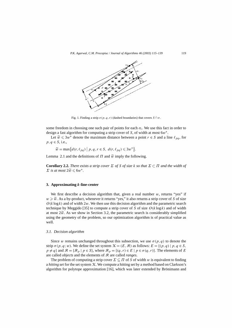
pq is the horizontal line throughp. For any three, not necessarily distinct, pointsp,q, r inthe plane, we denote byσ(p,q, r) the strip of width 2· d(r, pq) havingpq as the medianline. If r ∈ pq , σ(p,q, r) is the same aspq . Let Π = σ(p,q, r) | p,q, r ∈ S. We alsouse the notationσ(p,q;w) to denote the strip of width 2w whose median line ispq.
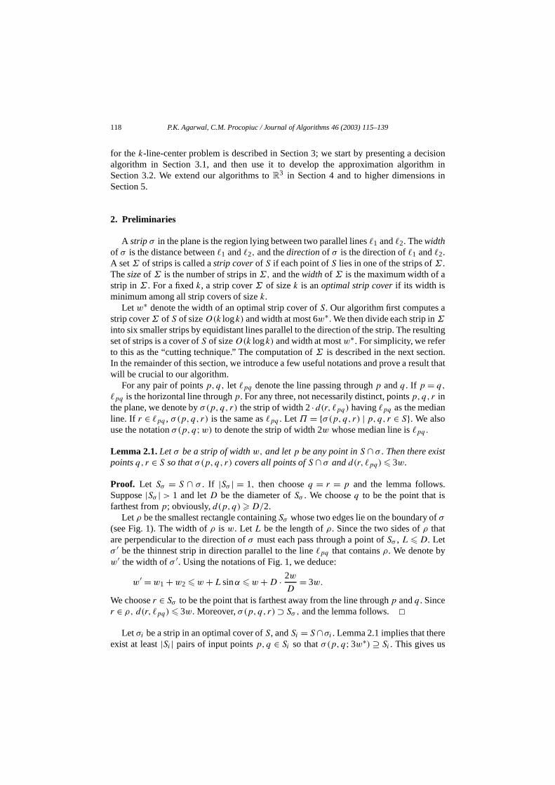
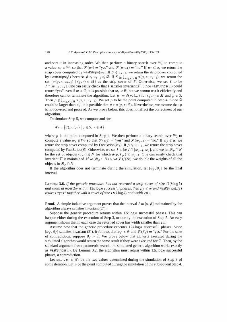
Lemma 2.1. Letσ be a strip of widthw, and letp be any point inS ∩ σ . Then there exispointsq, r ∈ S so thatσ(p,q, r) covers all points ofS ∩ σ andd(r, pq) 3w.
Proof. Let Sσ = S ∩ σ . If |Sσ | = 1, then chooseq = r = p and the lemma followsSuppose|Sσ | > 1 and letD be the diameter ofSσ . We chooseq to be the point that isfarthest fromp; obviously,d(p,q) D/2.
Let ρ be the smallest rectangle containingSσ whose two edges lie on the boundary oσ(see Fig. 1). The width ofρ is w. Let L be the length ofρ. Since the two sides ofρ thatare perpendicular to the direction ofσ must each pass through a point ofSσ , L D. Letσ ′ be the thinnest strip in direction parallel to the linepq that containsρ. We denote byw′ the width ofσ ′. Using the notations of Fig. 1, we deduce:
w′ =w1 +w2 w +Lsinα w+D · 2w
D= 3w.
We chooser ∈ Sσ to be the point that is farthest away from the line throughp andq . Sincer ∈ ρ, d(r, pq) 3w. Moreover,σ(p,q, r)⊃ Sσ , and the lemma follows.
Let σi be a strip in an optimal cover ofS, andSi = S ∩σi . Lemma 2.1 implies that therexist at least|Si | pairs of input pointsp,q ∈ Si so thatσ(p,q;3w∗) ⊇ Si . This gives us
P.K. Agarwal, C.M. Procopiuc / Journal of Algorithms 46 (2003) 115–139 119
o
arch
lifiedue as
on’sand
Fig. 1. Finding a stripσ(p,q, r) (dashed boundaries) that coversS ∩ σ .
some freedom in choosing one such pair of points for eachσi . We use this fact in order tdesign a fast algorithm for computing a strip cover ofS, of width at most 6w∗.
Let w 3w∗ denote the maximum distance between a pointr ∈ S and a linepq , forp,q ∈ S, i.e.,
w = maxd(r, pq)
∣∣ p,q, r ∈ S, d(r, pq) 3w∗.Lemma 2.1 and the definitions ofΠ andw imply the following.
Corollary 2.2. There exists a strip coverΣ of S of sizek so thatΣ ⊂Π and the width ofΣ is at most2w 6w∗.
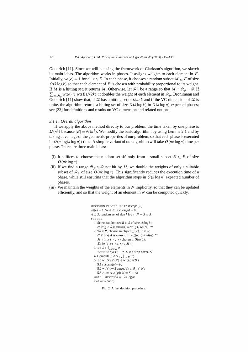
3. Approximating k-line-center
We first describe a decision algorithm that, given a real numberw, returns “yes” ifw w. As a by-product, whenever it returns “yes,” it also returns a strip cover ofS of sizeO(k logk) and of width 2w. We then use this decision algorithm and the parametric setechnique by Meggido [35] to compute a strip cover ofS of sizeO(k logk) and of widthat most 2w. As we show in Section 3.2, the parametric search is considerably simpusing the geometry of the problem, so our optimization algorithm is of practical valwell.
3.1. Decision algorithm
Sincew remains unchanged throughout this subsection, we useσ(p,q) to denote thestripσ(p,q;w). We define the set systemX = (E,R) as follows:E = (p, q) | p,q ∈ S,
p = q andR = Rp | p ∈ S, whereRp = (q, r) ∈E | p ∈ σ(q, r). The elements ofEare calledobjectsand the elements ofR are calledranges.
The problem of computing a strip coverΣ ⊆Π of S of widthw is equivalent to findingahitting setfor the set systemX. We compute a hitting set by a method based on Clarksalgorithm for polytope approximation [16], which was later extended by Brönimann
120 P.K. Agarwal, C.M. Procopiuc / Journal of Algorithms 46 (2003) 115–139
etcht in
t.
;
ase isby
xecuted
lef af
d
Goodrich [11]. Since we will be using the framework of Clarkson’s algorithm, we skits main ideas. The algorithm works in phases. It assigns weights to each elemenE.Initially, wt(e)= 1 for all e ∈E. In each phase, it chooses a random subsetM ⊆E of sizeO(k logk) so that each element ofE is chosen with probability proportional to its weighIf M is a hitting set, it returnsM. Otherwise, letRp be a range so thatM ∩ Rp = ∅. If∑
e∈Rpwt(e) wt(E)/(2k), it doubles the weight of each element inRp. Brönimann and
Goodrich [11] show that, ifX has a hitting set of sizek and if the VC-dimension ofX isfinite, the algorithm returns a hitting set of sizeO(k logk) in O(k logn) expected phasessee [23] for definitions and results on VC-dimension and related notions.
3.1.1. Overall algorithmIf we apply the above method directly to our problem, the time taken by one ph
Ω(n2) because|E| =Θ(n2). We modify the basic algorithm, by using Lemma 2.1 andtaking advantage of the geometric properties of our problem, so that each phase is ein O(n log(k logn)) time. A simpler variant of our algorithm will takeO(nk logn) time perphase. There are three main ideas:
(i) It suffices to choose the random setM only from a small subsetN ⊂ E of sizeO(nk logn).
(ii) If we find a rangeRp ∈ R not hit byM, we double the weights of only a suitabsubset ofRp of sizeO(nk logn). This significantly reduces the execution time ophase, while still ensuring that the algorithm stops inO(k logn) expected number ophases.
(iii) We maintain the weights of the elements inN implicitly, so that they can be updateefficiently, and so that the weight of an element inN can be computed quickly.
DECISIONPROCEDUREFastStrips(w)
wt(e) = 1, ∀e ∈E; successful= 0;A⊂ S: random set of sizek logn; N = S ×A;repeat
1. Select random setR ⊂ S of sizeck logk;/* Pr[q ∈ S is chosen] = wt(q)/wt(N). */
2. ∀q ∈ R, choose an object(q, r), r ∈A;/* Pr[r ∈A is chosen] = wt((q, r))/wt(q). */M: (q, r) | (q, r) chosen in Step 2;Σ : σ(q, r) | (q, r) ∈M;
3.if S ⊂ ⋃σ∈Σ σ
return “yes”; /* Σ is a strip cover. */4. Computep ∈ S \⋃
σ∈Σ σ ;5.if wt(Rp ∩N) wt(E)/(2k)
5.1successful++;5.2 wt(e) := 2wt(e), ∀e ∈ Rp ∩N ;5.3A :=A∪ p; N = S ×A;
until successful= 12k logn;return “no”;
Fig. 2. A fast decision procedure.
P.K. Agarwal, C.M. Procopiuc / Journal of Algorithms 46 (2003) 115–139 121
e thea
nd
stuting
l
ip
,
t
The algorithm is described in Fig. 2. We need the following notation. We definweight functionwt :E → Z
+. Initially, wt(e)= 1 for all e ∈E. The algorithm maintainssetA⊆ S so that the random set of objectsM is chosen from the setN = S ×A. Duringthe execution, new points may be added toA, but they are never deleted fromA. For anypointp ∈ S, we define wt(p) = ∑
q∈A wt((p, q)). We deduce that∑
p∈S wt(p) = wt(N).The weights wt(p) are updated every time the setA changes. The setM is computed intwo steps (Steps 1 and 2). To simplify notation, we denote byΣ the set of stripsσ(q, r),where(q, r) ∈ M. We say that a phase issuccessfulif Steps 5.1–5.3 are executed, aunsuccessfulotherwise.
3.1.2. CorrectnessWe prove that the decision procedure always returns “yes” ifw w, although it may
return “yes” even ifw < w.
Let S be a set ofn points in the plane, and letΣ∗ = σ ∗1 , . . . , σ
∗k be an optimal strip
cover ofS. We define thestrip subsetsof S with respect toΣ∗ to be the sets
S∗i =
p ∈ S∣∣ p ∈ σ ∗
i andp /∈ σ ∗j , ∀j < i
.
Thus,S∗1, . . . , S
∗k partitionS.
We prove that, for any 1 m k, the setA intersects at leastm+1 distinct strip subsetafter 12m logn successful phases, providedw w.1 As there are onlyk strip subsets, ifollows that the decision algorithm must terminate (and return “yes”) before exec12k logn successful phases.
Lemma 3.1. Let w w be a real number. For any positive integerm k, the setAintersects at leastm + 1 distinct strip subsets after the decision procedureFastStrips(w)
has executed12m logn successful phases.
Proof. Let x = 12m logn. For any 0 s x, let As denote the setA after s successfuphases. Clearly,As1 ⊆ As2 for anys1 s2. Suppose on the contrary,Ax intersects onlyjstrip subsets,j m. Since
⋃S∗i = S andA0 ⊆ Ax , the setAx intersects at least one str
subset, hencej 1. Without loss of generality, supposeAx intersectsS∗1, . . . , S
∗j and is
disjoint fromS∗j+1, . . . , S
∗k .
Let ri ∈ Ax ∩ S∗i ,1 i j , bej points so thatri is the first point ofS∗
i that is addedto A in Step 5.3 of the algorithm. By this we mean that eitherri ∈ A0 ∩ S∗
i , or thereexists 1 s x so thatri ∈ S∗
i ∩ (As \ As−1) andS∗i ∩ As−1 = ∅. Using Lemma 2.1
the definition ofw, and the fact thatw w, we can prove that there existj pointsq1, . . . , qj ∈ S so thatσ(qi, ri ) ⊃ S∗
i ,1 i j . For 1 s x, let ps be the point
computed in Step 4 of thesth successful phase. Thenps ∈ ⋃j
i=1S∗i (sinceps ∈ Ax and
Ax does not intersectS∗j+1, . . . , S
∗k ). Let S∗
i be the strip subset containingps, i j . If
ri ∈ As−1, then wt((qi, ri )) is doubled, because(qi, ri ) ∈ N ∩ Rps . Otherwise,ps = ri .For 1 i j , we denote byxi the number of times wt((qi, ri )) is doubled during the firs
1 The base of all logarithms is 2 unless stated explicitly.
122 P.K. Agarwal, C.M. Procopiuc / Journal of Algorithms 46 (2003) 115–139
putes
et
is
x successful phases. The observation above implies that∑j
i=1xi x − j . Since wt(E)
increases by a factor of at most(1+ 1/(2k)) after each successful phase, after 12m lognsuccessful phases we have
j∏i=1
wt((qi, ri ))
wt(E)
j∏i=1
2xi
n2(1+ 1/2k)x 2x−j
n2jejx/2k.
Then
log
(2x−j
n2jejx/(2k)
)= x − j − 2j logn− j loge
2kx
=(
1− j loge
2k
)· x − j − 2j logn
>
(1− loge
2
)· 3
1− 12 loge
m logn−m− 2m logn
> 0
(recall thatx = 12m logn and thatj m). Hence
j∏i=1
wt((qi, ri ))
wt(E)> 1.
This implies that for at least onei we have wt((qi, ri )) > wt(E), a contradiction. Lemma 3.1 immediately implies the following:
Lemma 3.2. For any valuew w, the decision procedureFastStrips(w) returns “yes”within 12k logn successful phases. Whenever it returns “yes,” the procedure also coma cover ofS of sizeO(k logk) and width2w.
Remark 3.3. The proof of Lemma 3.1 implies that there exists a setA of sizeO(k logn)
so that a strip cover ofS of size k and width at most 2w can be chosen from the sσ(q, r,p) | p,q ∈ S, r ∈A. However, we do not know how to computew andA directly.
3.1.3. Running timeFor anyr ∈A, the object(q, r) is selected with probability wt((q, r))/wt(N). Applying
the result from theε-net theory [23] to the set system induced byR on N (which has afinite VC-dimension), we have that
Pr[wt(Rp ∩N) wt(N)/(2k)
] 1/2.
Since wt(N) wt(E), we deduce
Pr[wt(Rp ∩N) wt(E)/(2k)
] 1/2.
Thus, a phase is successful with probability at least 1/2. The expected number of phasesO(k logn).
P.K. Agarwal, C.M. Procopiuc / Journal of Algorithms 46 (2003) 115–139 123
ke thea
the
g the
rt the
e
ed tree
e
vals
We now analyze the time required by each phase. To simplify the analysis, we maassumption thatk2 logk n. Let a = |A| =O(k logn). A naïve algorithm for executingphase takesO(na) time. Such an algorithm simply checks for eachp ∈ S and(q, r) ∈ M
whetherp ∈ σ(q, r). If p is not covered and wt(N ∩ Rp) wt(E)/2k (which we checkby looking at all elements inN ∩ Rp), we double the weights for all objects inN ∩ Rp .We now show how each phase can be executed inO(n loga) time.
First, let us consider Step 3. LetM be the set of objects chosen in Step 2. ComputearrangementA of the lines that form the boundaries of the stripsσ(q, r), for all (q, r) ∈M;mark every cell ofA that is contained in at least one stripσ(q, r), (q, r) ∈ M. Usingan optimal planar point-location algorithm [18], for each pointp ∈ S, find the cell ofAthat containsp. If the cell is marked,p is covered by at least one strip; otherwise,p isnot covered by any strip. Obviously, this also solves Step 4. The time for computinarrangementA is O(|M|2)=O(k2 log2 k)=O(n logk) sincen k2 logk, and we spendO(n logk) time to locate all points. Thus, Steps 3 and 4 are executed inO(n logk) time.
3.1.4. Data structuresTo implement Steps 1, 2, and 5 efficiently, we use data structures that suppo
following three operations:
(i) Return a pointq in S with probability wt(q)/wt(N).
(ii) Given a pointq ∈ S, return an object(q, r), r ∈A, with probability wt((q, r))/wt(q).(iii) For a given pairp,q ∈ S, double the weights of all objects in the set
Rpq = (q, r) ∈N
∣∣ p ∈ σ(q, r).
For each pointq ∈ S, we maintain a dynamic segment treeTq as explained below. Thunderlying structure of a dynamic segment tree is a weightedBB[α]-tree. Since we donot need the full functionality of a dynamic segment tree, we use a less sophisticatstructure, such as ared-blacktree.
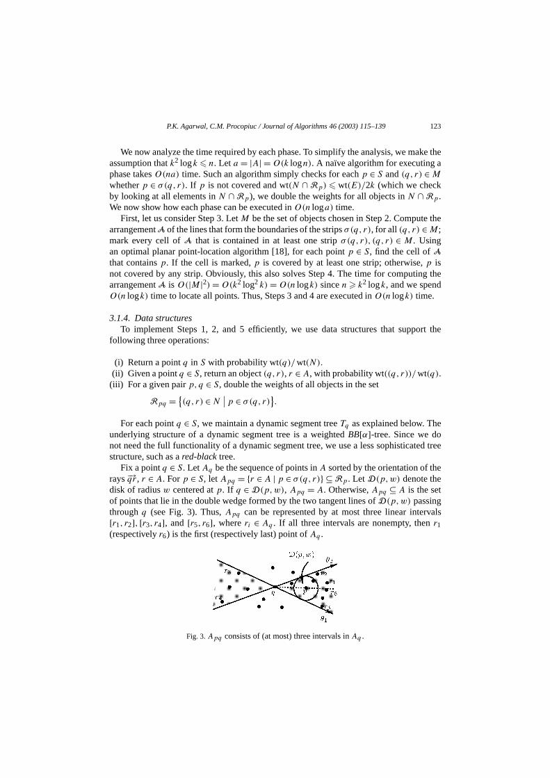
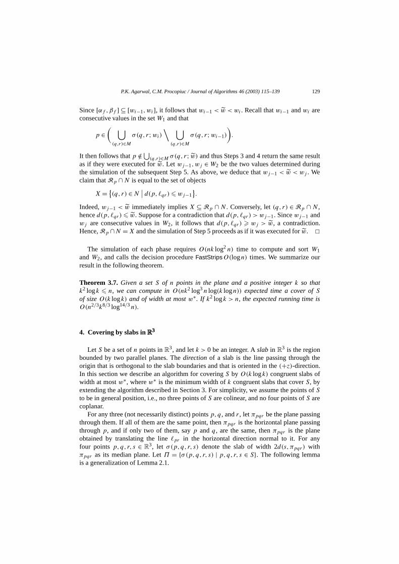
Fix a pointq ∈ S. LetAq be the sequence of points inA sorted by the orientation of thrays−→qr, r ∈A. Forp ∈ S, letApq = r ∈A | p ∈ σ(q, r) ⊆ Rp . Let D(p,w) denote thedisk of radiusw centered atp. If q ∈ D(p,w), Apq = A. Otherwise,Apq ⊆ A is the setof points that lie in the double wedge formed by the two tangent lines ofD(p,w) passingthroughq (see Fig. 3). Thus,Apq can be represented by at most three linear inter[r1, r2], [r3, r4], and [r5, r6], whereri ∈ Aq . If all three intervals are nonempty, thenr1(respectivelyr6) is the first (respectively last) point ofAq .
Fig. 3.Apq consists of (at most) three intervals inAq .
124 P.K. Agarwal, C.M. Procopiuc / Journal of Algorithms 46 (2003) 115–139
dded toe
ith
ntlerted,
ofIt
he
oficf
th
ee
st
e. If
ator in
ion,totic
Thatthistraverse
Let Jq be the set of intervals representing the subsetsApq , wherep is a point reportedin Step 4 of a successful phase. After each successful phase, at most one point is aAq and at most three new intervals are added toJq . We storeJq in a dynamic segment treTq to maintain the weights of objects(q, r), r ∈ Aq . The leaves ofTq are labeled by thepoints inAq in increasing order from left to right. For simplicity, we identify a leaf wits label. Each interior nodev of Tq is associated with a canonical setSv , which is the setof all points inAq associated with the leaves of the subtree rooted atv. Each nodev is alsoassociated with a subset of intervalsJ v
q ⊆ Jq . Instead of storingJ vq explicitly atv, we will
simply store the number of intervals inJ vq , i.e., the valuekv = |J v
q |. In a standard segmetree an intervalJ is stored at a nodev if Sv ⊆ J butSp(v) ⊆ J . When we insert an intervainto Tq we will use the same rule, but later, as other points and intervals are being inswe will not enforce the above condition, in the sense thatJ might be stored at a nodeveven ifSp(v) ⊆ J . The reason is that, as the structure ofTq changes due to the insertionnew points intoAq , we have to perform rotations onTq to keep it balanced (see below).is expensive to update the setJ v
q during rotations. However, we will always maintain tfollowing invariant:
(-) If an intervalJ is stored at nodesv1, . . . , vk , thenJ = ⋃ki=1Svi andSvi ∩ Svj = ∅.
If Tq were static, the invariant above would imply that the weight wt((q, r)) of any pair
(q, r) ∈ S ×A can be computed as 2∑
y ky , where the summation is taken over all nodesTq on the path from the root to the leaf labeledr. However, this does not hold for a dynamtree: when adding a new leafr ′ to Tq , the weight wt((q, r ′)) is always 1, irrespective ohow many intervals are already stored in the nodes from the root tor ′. To solve this, weassociate a valuewv to each nodev of Tq such that
wv =∑
r wt((q, r))
2∑
y ky, (1)
wherer ranges over all leaves in the subtree ofv, andy ranges over all nodes on the pafrom the root to the parent ofv. In the following, we use the notationΠv to denote the pathin Tq from the root to the parent ofv. Initially, wv is the number of leaves in the subtr
of v. When inserting a new leafr ′, we setwr ′ = 1/2∑
y ky , wherey ranges over all nodeonΠr ′ . We also update the valueswv for the ancestors ofr ′, as detailed below. Note tha(1) implieswroot= wt(q).
An interval [ri, rj ] is inserted intoTq using the standard segment tree proceduran interval is stored at an ancestor ofv, then all leaves in the subtree rooted atv lie inthis interval, so their weights double. Since both the numerator and the denominthe expression ofwv increase by a factor of 2,wv does not change. Thus,wv changesonly when an interval is stored atv or at one of its descendents. Using this observatthe valueswv can be updated while inserting an interval, without affecting the asymprunning time of the segment-tree insertion procedure.
A point is inserted intoAq using the standard red-black tree insertion procedure.is, we first traverse a path ofTq from the root to a leaf and insert the new point there;is called the top-down phase. In the second phase, called the bottom-up phase, we

P.K. Agarwal, C.M. Procopiuc / Journal of Algorithms 46 (2003) 115–139 125
the
. 4that
ode.
w
are
wv0 :=wv0 + 1;P = 1; k = kv0;for i = 1 to h dobegin
P := P · 2kvi−1 ;wvi :=wvi + 1/P ;k := k + kvi ;
end
kτ := 0; wτ := 1
2k;
Fig. 4. Updating valueswv in the top-down phase.
kc := kc + ky ;wc :=wc · 2ky ;kb := kb + ky ;wb :=wb · 2ky ;ky := kx; kx := 0;wx :=wa +wb;wy := 2ky (wx +wc);
Fig. 5. Maintaining valueskv andwv under left rotation.
the same path backwards and performO(1) rotations to rebalance the tree. In each oftwo phases, the valueskv andwv are updated as follows.
Let τ be the new leaf that was created to insert a new pointr in Aq , and letΠτ =v0, v1, . . . , vh be the path from the root to the parent ofτ . The procedure described in Figupdates the valueswv in O(loga) time during the top-down phase. It can be checkedthe values stored at the nodes after the top-down phase satisfy (1).
In the bottom-up phase, suppose we perform a left rotation at a nodev. Figure 5describes the structural change inTq and the update of the values stored at each nIntuitively, J
yq , the set of intervals stored aty, is pushed to its childrenb and c, i.e.,
J bq := J b
q ∪ Jyq andJ c
q := J cq ∪ J
yq . Since the setSy after the rotation is the same asSx
before the rotation, we moveJ xq to J
yq and setJ x
q = ∅. It can be checked that the nevalues stored at the nodesx, y, a, b, andc after the rotation satisfy (1).
3.1.5. Details of the algorithmWith this definition for the treesTq , Steps 1 and 2, as well as the test in Step 5
executed as follows.
Step1. Check the roots of all segment trees and pick the pointsq ∈ S with probabilitywroot(Tq)/wt(N), where wt(N) = ∑
q∈S wroot(Tq). Choosing one pointq ∈ S can be donein O(logn) time, so the total time for this step isO(k logk logn).
Step2. For each pointq ∈ R, we want to choose an object(q, r), r ∈A, with probabilitywt((q, r))/wt(q). Let rk(r) denote the rank ofr in the orderAq . We choose a random
126 P.K. Agarwal, C.M. Procopiuc / Journal of Algorithms 46 (2003) 115–139
n we
d
rmineingin
lue
ion
numberm between 1 and wt(q) with uniform probability and then traverseTq to determinethe leafr ∈Aq such that∑
r ′∈Aq
rk(r ′)<rk(r)
wt((q, r ′)
)<m and
∑r ′∈Aq
rk(r ′)rk(r)
wt((q, r ′)
) m. (2)
The object(q, r) is returned. The traversal procedure maintains the invariant that wheare at a nodev, we are given the valueµv = 2
∑y∈Πv
ky and an integermv ∈ [1,µvwv],and we want to return a point ofAq that satisfies (2) form = mv and forr ′ ranging onlyover the points in the subtree rooted atv. If v is a leaf, thenr is the point associatewith v. Otherwise, letu andz be the left and right children ofv. Letµu = µz = µv2kv . Ifmv µuwu, then we visitu with mu =mv . Otherwise, we visitz with mz =mv −µuwu.We spendO(1) time per visited node. Hence, this step takesO(k log(k) loga) time, overall O(k logk) pointsq ∈R.
Step5. First we describe the execution of Step 5.2, and then we explain how to detethe test in Step 5. Letp be the point computed in Step 4. In view of the preceddiscussion, for each pointq ∈ S we want to returnApq as at most three linear intervalsthe sorted sequenceAq . Let θ1, θ2 be the orientations of the two tangent lines ofD(p,w)
passing throughq . Since the leaves ofTq are sorted by the orientation of points inA withrespect toq , we can compute the required intervals inO(loga) time by searchingTq withθ1 andθ2. We then insert these intervals inTq and addp as a leaf inTq . The total timespent in Step 5.2 isO(n loga).
It remains to describe how to execute the test in Step 5. For a fixed pointq ∈ S, letI1, I2, I3 be the three intervals representingApq as discussed above. We compute the va∑
r∈Apqwt((q, r)) as follows. LetI be one of the three intervals above. We traverseTq
to find the nodes associated withI , and we use the valueskv andwv and (1) to computew(I)= ∑
r∈I wt((q, r)). Then,∑r∈Apq
wt((q, r)
) =w(I1)+w(I2)+w(I3).
Finally,
wt(Rp)=∑q∈S
∑r∈Apq
wt((q, r)
).
The time required for computing wt(Rp) is thusO(n loga).Taking into account the fact that the decision procedure terminates afterO(k logn)
successful phases, we conclude with the following.
Theorem 3.4. For any real numberw 0, the expected running time of the decisalgorithm FastStrips(w) is O(nk log(n) log(k logn)) (assumingk2 logk n). If w w,
FastStrips(w) returns “yes,” together with a cover ofS by O(k logk) strips of width atmost2w.
P.K. Agarwal, C.M. Procopiuc / Journal of Algorithms 46 (2003) 115–139 127
nt] to
d
eset
y
tor
wof our
y
coverat
d on the
Remark 3.5. If k2 logk > n, we modify the implementation of Step 3, as it is inefficieto compute the entire arrangementA. Instead we use the algorithm described in [1,14determine whetherS lies in the union of the strips inΣ . This step takes
O(|Σ|2/3n2/3 logn
) =O(k2/3n2/3 log5/3n
)time. A phase can thus be implemented inO(n2/3k2/3 log5/3n) time, and the expecterunning time of the decision algorithm isO(n2/3k5/3 log8/3n).
3.2. Optimization algorithm
We are now ready to describe our algorithm that, given a set ofn points in theplane, computes a strip coverΣ of S of sizeO(k logk) and width at most 2w 6w∗.Using the “cutting technique” as outlined in Section 2, we can then transformΣ into anew coverΣ ′ of sizeO(k logk) and width at mostw∗. In view of Remark 3.3, therexists a subsetA ⊆ S of sizeO(k logn) so thatΣ can be chosen as a subset of theσ(q, r,p) | p,q ∈ S, r ∈ A. If we could computeA efficiently, we could do a binarsearch on the set
W = d(p, qr )
∣∣ p,q ∈ S, r ∈A,
using the decision procedureFastStrips(w) at each step. However, we do not know howcomputeA efficiently, as it depends on the unknown valuew. By Corollary 2.2, anothepossibility is to chooseΣ as a subset ofΠ = σ(q, r,p) | p,q, r ∈ S. But in this casewe have to do a binary search on the setd(p, qr ) | p,q, r ∈ S, and we do not knowhow to choose an element of given rank from this set in timeo(n2). Our solution is to dobinary searches on appropriate subsets ofW that we can compute efficiently. We borroideas from Meggido’s parametric searching technique [35] and exploit the geometryproblem to compute these subsets efficiently.
Our goal is to simulate the decision procedureFastStrips(w) generically atw, withoutknowing the value ofw. To simplify notation, letF (w) denote the result returned bFastStrips(w). The algorithm maintains an intervalI = [α,β] that satisfies the followinginvariant:
[α,β] = ∅, α < w, and F (β)= “yes.” (I ′)
Initially, I = [−∞,+∞]. SinceFastStrips(w) could returnyes even ifw < w, unlike thestandard parametric searching,w is not guaranteed to lie in the interval[α,β]. The genericalgorithm will not be able to detect immediately when it tries to setβ to a value less thanw.If this happens, then the generic algorithm will no longer be simulatingFastStrips at w.The generic algorithm will either detect the situation at a later stage and return a stripof width at most 2w, or it will finish the simulation. In the latter case, we will argue thβ w. We simulate the simpler version of the decision procedure that takesO(nk logn)
time per phase and does not maintain segment trees. Steps 1 and 2 do not depenvaluew. We describe the simulation of Steps 3, 4, and 5 below.
In order to simulate Steps 3 and 4, we compute the set
W1 = d(p, qr )
∣∣ p ∈ S, (q, r) ∈M
128 P.K. Agarwal, C.M. Procopiuc / Journal of Algorithms 46 (2003) 115–139
d
d
tof our
r
ate
aneasy
ce
the
exactlyl
3 oftep 4.
and sort it in increasing order. We then perform a binary search overW1 to computea valuewi ∈ W1 so thatF (wi) = “yes” andF (wi−1) = “no.” If wi α, we return thestrip cover computed byFastStrips(wi). If β wi−1, we return the strip cover computeby FastStrips(β) becauseβ wi−1 w. If S ⊆ ⋃
(q,r)∈M σ(q, r;wi−1), we return theset σ(q, r;wi−1) | (q, r) ∈ M as the strip cover ofS. Otherwise, we setI to beI ∩[wi−1,wi]. One can easily check thatI satisfies invariantI ′. SinceFastStrips(w) couldreturn “yes” even ifw < w, it is possible thatwi < w, but we cannot test it efficiently antherefore cannot terminate the algorithm. Letwi = d(p, qr ) for (q, r) ∈ M andp ∈ S.Thenp /∈ ⋃
(q,r)∈M σ(q, r;wi−1). We setp to be the point computed in Step 4. Sincew
could be larger thanwi , it is possible thatp ∈ σ(q, r; w). Nevertheless, we assume thapis not covered and proceed. As we prove below, this does not affect the correctnessalgorithm.
To simulate Step 5, we compute and sort
W2 = d(p, qr )
∣∣ q ∈ S, r ∈A
wherep is the point computed in Step 4. We then perform a binary search overW2 tocompute a valuewj ∈ W2 so thatF (wj ) = “yes” andF (wj−1) = “no.” If wj α, wereturn the strip cover computed byFastStrips(wj ). If β wj−1, we return the strip covecomputed byFastStrips(β). Otherwise, we setI to beI ∩ [wj−1,wj ], and we letRp ∩N
be the set of objects(q, r) ∈ N for which d(p, qr ) wj−1. One can easily check thinvariantI ′ is maintained. If wt(Rp ∩N) wt(E)/(2k), we double the weights of all thobjects inRp ∩N .
If the algorithm does not terminate during the simulation, let[αf ,βf ] be the finalinterval.
Lemma 3.6. If the generic procedure has not returned a strip cover of sizeO(k logk)
and width at most2w within 12k logn successful phases, thenβf w andFastStrips(βf )
returns “yes” together with a cover of sizeO(k logk) and width2βf .
Proof. A simple inductive argument proves that the intervalI = [α,β] maintained by thealgorithm always satisfies invariant (I ′).
Suppose the generic procedure returns within 12k logn successful phases. This chappen either during the execution of Step 3, or during the execution of Step 5. Anargument shows that in each case the returned cover has width smaller than 2w.
Assume now that the generic procedure executes 12k logn successful phases. Sin[αf ,βf ] satisfies invariant (I ′), it follows thatαf < w andF (βf ) = “yes.” For the sakeof contradiction, supposeβf > w. We prove below that all tests executed duringsimulated algorithm would return the same result if they were executed forw. Then, by thestandard argument from parametric search, the simulated generic algorithm worksas FastStrips(w). By Lemma 3.2, the algorithm must return within 12k logn successfuphases, a contradiction.
Let wi−1,wi ∈ W1 be the two values determined during the simulation of Stepsome iteration. Letp be the point computed during the simulation of the subsequent S
P.K. Agarwal, C.M. Procopiuc / Journal of Algorithms 46 (2003) 115–139 129
sultg
.
r
is
he
f
s of
gg
y
Since[αf ,βf ] ⊆ [wi−1,wi], it follows thatwi−1 < w < wi . Recall thatwi−1 andwi areconsecutive values in the setW1 and that
p ∈( ⋃
(q,r)∈Mσ(q, r;wi)
∖ ⋃(q,r)∈M
σ(q, r;wi−1)
).
It then follows thatp /∈ ⋃(q,r)∈M σ(q, r; w) and thus Steps 3 and 4 return the same re
as if they were executed forw. Let wj−1,wj ∈ W2 be the two values determined durinthe simulation of the subsequent Step 5. As above, we deduce thatwj−1 < w < wj . Weclaim thatRp ∩N is equal to the set of objects
X = (q, r) ∈N
∣∣ d(p, qr ) wj−1.
Indeed,wj−1 < w immediately impliesX ⊆ Rp ∩ N . Conversely, let(q, r) ∈ Rp ∩ N ,henced(p, qr ) w. Suppose for a contradiction thatd(p, qr ) > wj−1. Sincewj−1 andwj are consecutive values inW2, it follows that d(p, qr ) wj > w, a contradictionHence,Rp ∩N =X and the simulation of Step 5 proceeds as if it was executed forw.
The simulation of each phase requiresO(nk log2n) time to compute and sortW1andW2, and calls the decision procedureFastStripsO(logn) times. We summarize ouresult in the following theorem.
Theorem 3.7. Given a setS of n points in the plane and a positive integerk so thatk2 logk n, we can compute inO(nk2 log3n log(k logn)) expected time a cover ofSof sizeO(k logk) and of width at mostw∗. If k2 logk > n, the expected running timeO(n2/3k8/3 log14/3n).
4. Covering by slabs in R3
R3
R3
Let S be a set ofn points inR3, and letk > 0 be an integer. Aslab in R
3 is the regionbounded by two parallel planes. Thedirection of a slab is the line passing through torigin that is orthogonal to the slab boundaries and that is oriented in the(+z)-direction.In this section we describe an algorithm for coveringS by O(k logk) congruent slabs owidth at mostw∗, wherew∗ is the minimum width ofk congruent slabs that coverS, byextending the algorithm described in Section 3. For simplicity, we assume the pointS
to be in general position, i.e., no three points ofS are colinear, and no four points ofS arecoplanar.
For any three (not necessarily distinct) pointsp,q , andr, let πpqr be the plane passinthrough them. If all of them are the same point, thenπpqr is the horizontal plane passinthroughp, and if only two of them, sayp andq , are the same, thenπpqr is the planeobtained by translating the linepr in the horizontal direction normal to it. For anfour pointsp,q, r, s ∈ R
3, let σ(p,q, r, s) denote the slab of width 2d(s,πpqr) withπpqr as its median plane. LetΠ = σ(p,q, r, s) | p,q, r, s ∈ S. The following lemmais a generalization of Lemma 2.1.
130 P.K. Agarwal, C.M. Procopiuc / Journal of Algorithms 46 (2003) 115–139
llel
Fig. 6. Bounding the width of a slab, in a given direction, that containsP .
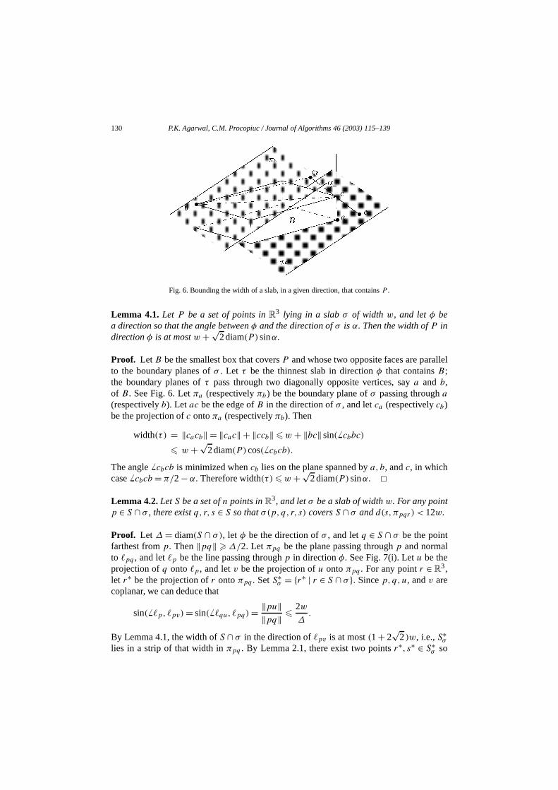
Lemma 4.1. Let P be a set of points inR3 lying in a slabσ of width w, and letφ bea direction so that the angle betweenφ and the direction ofσ is α. Then the width ofP indirectionφ is at mostw+√
2diam(P )sinα.
Proof. Let B be the smallest box that coversP and whose two opposite faces are parato the boundary planes ofσ . Let τ be the thinnest slab in directionφ that containsB;the boundary planes ofτ pass through two diagonally opposite vertices, saya and b,of B. See Fig. 6. Letπa (respectivelyπb) be the boundary plane ofσ passing througha(respectivelyb). Let ac be the edge ofB in the direction ofσ , and letca (respectivelycb)be the projection ofc ontoπa (respectivelyπb). Then
width(τ ) = ‖cacb‖ = ‖cac‖+ ‖ccb‖ w + ‖bc‖sin( cbbc) w +√
2diam(P )cos( cbcb).
The angle cbcb is minimized whencb lies on the plane spanned bya, b, andc, in whichcase cbcb = π/2− α. Therefore width(τ ) w +√
2diam(P )sinα. Lemma 4.2. LetS be a set ofn points inR
3, and letσ be a slab of widthw. For any pointp ∈ S ∩ σ , there existq, r, s ∈ S so thatσ(p,q, r, s) coversS ∩ σ andd(s,πpqr ) < 12w.
Proof. Let ∆ = diam(S ∩ σ), let φ be the direction ofσ , and letq ∈ S ∩ σ be the pointfarthest fromp. Then‖pq‖ ∆/2. Letπpq be the plane passing throughp and normalto pq , and letp be the line passing throughp in directionφ. See Fig. 7(i). Letu be theprojection ofq ontop , and letv be the projection ofu ontoπpq . For any pointr ∈ R
3,let r∗ be the projection ofr ontoπpq . SetS∗
σ = r∗ | r ∈ S ∩ σ . Sincep,q,u, andv arecoplanar, we can deduce that
sin( p, pv)= sin( qu, pq)= ‖pu‖‖pq‖ 2w
∆.
By Lemma 4.1, the width ofS ∩ σ in the direction ofpv is at most(1+ 2√
2)w, i.e.,S∗σ
lies in a strip of that width inπpq . By Lemma 2.1, there exist two pointsr∗, s∗ ∈ S∗σ so
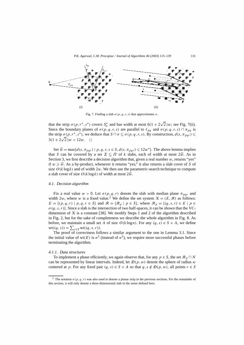
P.K. Agarwal, C.M. Procopiuc / Journal of Algorithms 46 (2003) 115–139 131
s
pute
e VC-ibed8. As
Sincefore
der of
(i) (ii)
Fig. 7. Finding a slabσ(p,q, r, s) that approximatesσ .
that the stripσ(p, r∗, s∗) coversS∗σ and has width at most 6(1+ 2
√2)w; see Fig. 7(ii).
Since the boundary planes ofσ(p,q, r, s) are parallel topq andσ(p,q, r, s) ∩ πpq isthe stripσ(p, r∗, s∗), we deduce thatS ∩ σ ⊆ σ(p,q, r, s). By construction,d(s,πpqr ) 3(1+ 2
√2)w < 12w.
Setw = maxd(s,πpqr) | p,q, r, s ∈ S,d(s,πpqr ) 12w∗. The above lemma impliethat S can be covered by a setΣ ⊆ Π of k slabs, each of width at most 2w. As inSection 3, we first describe a decision algorithm that, given a real numberw, returns “yes”if w w. As a by-product, whenever it returns “yes,” it also returns a slab cover ofS ofsizeO(k logk) and of width 2w. We then use the parametric-search technique to coma slab cover of sizeO(k logk) of width at most 2w.
4.1. Decision algorithm
Fix a real valuew > 0. Let σ(p,q, r) denote the slab with median planeπpqr andwidth 2w, wherew is a fixed value.2 We define the set systemX = (E,R) as follows:E = (p, q, r) | p,q, r ∈ S and R = Rp | p ∈ S, whereRp = (q, s, r) ∈ E | p ∈σ(q, s, r). Since a slab is the intersection of two half-spaces, it can be shown that thdimension ofX is a constant [38]. We modify Steps 1 and 2 of the algorithm descrin Fig. 2, but for the sake of completeness we describe the whole algorithm in Fig.before, we maintain a small setA of sizeO(k logn). For any(q, s) ∈ S × A, we definewt((q, s))= ∑
r∈S wt((q, s, r)).The proof of correctness follows a similar argument to the one in Lemma 3.1.
the initial value of wt(E) is n3 (instead ofn2), we require more successful phases beterminating the algorithm.
4.1.1. Data structuresTo implement a phase efficiently, we again observe that, for anyp ∈ S, the setRp ∩N
can be represented by linear intervals. Indeed, letD(p,w) denote the sphere of radiuswcentered atp. For any fixed pair(q, s) ∈ S × A so thatq, s /∈ D(p,w), all pointsr ∈ S
2 The notationσ(p,q, r) was also used to denote a planar strip in the previous sections. For the remainthis section, it will only denote a three-dimensional slab in the sense defined here.
132 P.K. Agarwal, C.M. Procopiuc / Journal of Algorithms 46 (2003) 115–139
de the
t
in
heee
DECISIONPROCEDUREFastslab(w)
wt(e)= 1,∀e ∈E; successful= 0;A⊂ S: random set of sizek logn; N = S ×A× S;repeat
1. Select random setR ⊂ S ×A of sizeck logk;/* Pr[(q, s) ∈ S ×A is chosen] = wt((q, s))/wt(N). */
2.∀(q, s) ∈ R, choose an object(q, s, r), r ∈ S;/* Pr[r ∈ S is chosen] = wt((q, s, r))/wt((q, s)). */M: (q, s, r) | (q, s, r) chosen in Step 2;Σ : σ(q, s, r) | (q, s, r) ∈M;
3.if S ⊂ ⋃σ∈Σ σ
return “yes”; /* Σ is a strip cover. */4. Computep ∈ S \⋃
σ∈Σ σ ;5.if wt(Rp ∩N) wt(E)/(2k)
5.1successful++;5.2 wt(e) := 2wt(e), ∀e ∈ Rp ∩N ;5.3A :=A∪ p; N = S ×A× S;
until successful= 16k logn;return “no”;
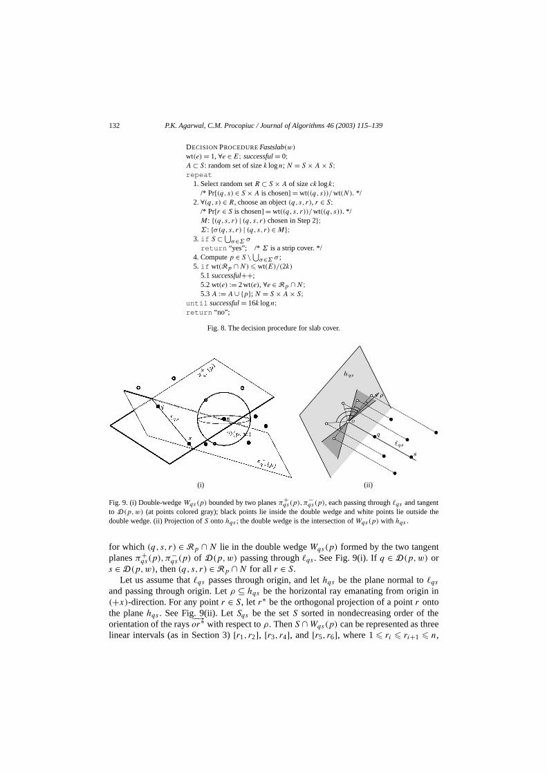
Fig. 8. The decision procedure for slab cover.
(i) (ii)
Fig. 9. (i) Double-wedgeWqs(p) bounded by two planesπ+qs(p),π
−qs(p), each passing throughqs and tangent
to D(p,w) (at points colored gray); black points lie inside the double wedge and white points lie outsidouble wedge. (ii) Projection ofS ontohqs ; the double wedge is the intersection ofWqs(p) with hqs .
for which (q, s, r) ∈ Rp ∩ N lie in the double wedgeWqs(p) formed by the two tangenplanesπ+
qs(p),π−qs(p) of D(p,w) passing throughqs . See Fig. 9(i). Ifq ∈ D(p,w) or
s ∈ D(p,w), then(q, s, r) ∈ Rp ∩N for all r ∈ S.Let us assume thatqs passes through origin, and lethqs be the plane normal toqs
and passing through origin. Letρ ⊆ hqs be the horizontal ray emanating from origin(+x)-direction. For any pointr ∈ S, let r∗ be the orthogonal projection of a pointr ontothe planehqs . See Fig. 9(ii). LetSqs be the setS sorted in nondecreasing order of torientation of the rays
−−→or∗ with respect toρ. ThenS ∩Wqs(p) can be represented as thr
linear intervals (as in Section 3)[r1, r2], [r3, r4], and [r5, r6], where 1 ri ri+1 n,
P.K. Agarwal, C.M. Procopiuc / Journal of Algorithms 46 (2003) 115–139 133
e
k-
in
n
the
mptoticanes
e,in
hors
st,
in the sense that all points ofSsq whose ranks are in the range[r1, r2] ∪ [r3, r4] ∪ [r5, r6]lie in Wqs(p). Note that unlike Section 3 in which we used the points ofA themselves torepresent the intervals, we now use the ranks of points inSqs to represent the intervals. Wneed a data structure that supports the following three operations:
(Q1) Given a pair(q, s) ∈ S ×A and a pointr ∈ S, return the rank ofr, rk(r), in Sqs .(Q2) Given a pair(q, s) ∈ S ×A and a half-planeπ bounded byqs , determine the ran
of the point thatπ meets first as we rotate it aroundqs in clockwise (or counterclockwise) direction.
(Q3) Given a pair(q, s) ∈ S×A and an integer 1 i n, return the point inSqs of ranki.
We fix a parameterm n3 and preprocessS in O(m logm) time into a partition-tree based data structureΨ of size O(m) that answers a simplex-range queryO((n/m1/3)polylog(n)) time [2]. Let γqs be the half-plane spanned byqs andρ, andfor a pointr ∈ S, letπqs(r) be the plane spanned byqs andr. If r ∈ qs , letπqs(r)= γqs .Then rk(r) in Sqs is determined by the numbernqs(r) of points lying in the wedgebounded byγqs and πqs(r) and that containsr. More precisely, if the angle betweeρ and
−−→or∗ in counterclockwise direction is at mostπ , then rk(r) = nqs(r). Otherwise,
rk(r) = n − nqs(r) + |γqs ∩ S| + 1. A (Q2) query can also be reduced to countingnumber of points lying in a wedge bounded byπ andγqs . As shown in [2], the simplexrange-counting query can also be used to answer a (Q3) query within the same asytime bound. Eachri can be computed by answering (Q2) queries for the four half-plcontained inπ+
qs(p), π−qs(p) and bounded byqs .
As in Section 3, we would like to maintain a segment treeTqs for each pair(q, s) ∈S × A to store the intervals representingWqs(p). SinceTqs stores intervals[ri, ri+1] ⊆[1, n], eachTqs would haven leaves—labeled 1 throughn from left to right—and thus thetotal space and time needed to maintain these trees explicitly would beΩ(n2k), which istoo expensive. We observe that onlyO(logn) nodes of eachTqs are visited in each phasso the decision algorithm visits a total ofO(kn logn) nodes in each phase. Keeping thismind, we maintain eachTqs implicitly, by explicitly representing only those nodes ofTqs
that have been accessed by the algorithm.In more detail, for each internal nodev of Tqs , we either explicitly represent bot
children of v or neither of them. Ifv is represented explicitly, then all of its ancestare also represented explicitly. We thus explicitly represent a top subtree ofTqs . The ithleftmost leaf ofTqs is labeledi and is associated with the point ofSqs whose rank isi.For each explicitly represented nodev, we store an integerkv , the number of intervalstored atv, and an interval[αv,βv] whereαv (respectivelyβv) is the label of the leftmos(respectively rightmost) leaf of the subtree rooted atv. If v is not explicitly representedthen kv = 0. We also store an integerωv at v, defined as follows. Ifv is a leaf, thenωv = 2kv . If v is an internal node with childrenu andz thenωv = 2kv (ωu + ωz). Hence,for any nodev, the following holds:
∑wt
((q, s, r)
) = ωv · 2∑
y∈Πvky , (4)
r
134 P.K. Agarwal, C.M. Procopiuc / Journal of Algorithms 46 (2003) 115–139
t
hm
r
ot
e
tgervals
is thattore
eet
wherer ranges over all points associated with the leaves in the subtree ofv, andΠv is thepath from the root to the parent ofv.
Since the setS does not change over time, unlike Section 3, the set of nodes inTqs
remains fixed. But whenever we add a point toA, n new trees are created.
4.1.2. Implementing a phaseWe now describe how we implement various steps of the decision algorithm.
Step1. If the rootu of Tqs is not explicitly represented, then no interval is stored inTqs
yet, so wt((q, s))= n. Otherwise,ωu = wt((q, s)). By examining allO(nk logn) trees, wecan determine wt((q, s)) for all (q, s) ∈ S ×A. Compute wt(N) = ∑
(q,s)∈S×A wt((q, s))and choose(q, s) ∈ S ×A with probability wt((q, s))/wt(N). Choosing a pair(q, s) canbe done inO(k log2n) time, so the total time spent in selectingR is O(k2 log(k) log2n).
Step2. For each point(q, s) ∈ R, we want to choose an object(q, s, r), for r ∈ S, withprobability wt((q, s, r))/wt((q, s)). We have already computed wt((q, s)) in Step 1. Wechoose a random integerm ∈ [1,wt((q, s))] with uniform probability and find the poinr ∈ Sqs such that∑
r ′∈Sqsrk(r ′)<rk(r)
wt((q, s, r ′)
)<m and
∑r ′∈Sqs
rk(r ′)rk(r)
wt((q, s, r ′)
) m. (5)
If the root of Tqs is not explicitly represented, then we simply return the point inSqsof rankm. Otherwise, we visitTqs in a top–down manner as in Section 3. The algorit
maintains the invariant that when we are at a nodev, we are given the valueµv = 2∑
y∈Πvky
and an integermv ∈ [1,µvωv], and we want to return a point ofSqs that satisfies (5) fom=mv and forr ′ ranging only over the points in the subtree rooted atv. If v is a leaf, thenwe return the point whose rank is stored atv. If v is an internal node but its children are nexplicitly represented, then we return the point ofSqs of rankαv+mv/(µv2kv )−1, usingthe data structureΨ mentioned above. Finally, letu andz be the left and right children ofv.Let µu = µz = µv2kv . If mv µuωu, then we visitu with mu =mv . Otherwise, we visitzwith mz =mv −µuωu.
We spendO((n/m1/3)polylog(n)) time for each pair(q, s) ∈ R, therefore the total timespent in Step 2 isO((nk/m1/3)polylog(n)).
Step5. The test in Step 5 is executed inO(nk logn) time in the same way as in thprocedure described in Section 3.1. In Step 5.2 we compute, for each(q, s) ∈ S×A, the (atmost) three intervals[r1, r2], [r3, r4], and[r5, r6], where 1 ri ri+1 n, that representhe points lying in the double wedgeWqs(p). Eachri is computed using the simplex ransearching data structureΨ as described above. We then insert each of these three intein Tqs using the standard segment-tree insertion procedure. The only differencewhen we try to access a nodev that is not explicitly represented, we create it and skv , ωv , and [αv,βv] at v. If v is the root ofTqs , thenαv = 1 andβv = n, otherwise ifv is the left (respectively right) child of its parentu, thenαv = αu,βv = (αu + βu)/2!(respectivelyαv = (αu + βu)/2! + 1, βv = βu). If v is a newly created node at which wstore an interval, we setkv = 1 andωv = 2(βv − αv + 1). For all other new nodes, we s
P.K. Agarwal, C.M. Procopiuc / Journal of Algorithms 46 (2003) 115–139 135
g
ecisioneion 3.2,
ina
s
e
dse
m
we
e-sts
Letmpareh
ns
,enericsteach
e of
kv = 0 andωv = βv − αv + 1. Note that we addp to A in Step 5.3 and createn new pairs(q,p) ∈ S ×A. Since no interval is stored inTqp, we do not create it. The overall runnintime of Step 5 isO((n2k/m1/3)polylog(n)).
Hence, the total expected running time of the decision algorithm over allO(k logn) suc-cessful phases, excluding the time spent in preprocessingΨ , isO((n2k2/m1/3)polylog(n)).
4.2. Optimization algorithm
We extend the parametric-search approach from the previous section to run the dalgorithm generically atw 12w∗. Steps 1 and 2 do not depend onw, so we can executthem as in the decision algorithm. Steps 3 and 4 are executed generically as in Sectby doing a binary search. Finally, in Step 5, we need the value ofw to compute, for eachpair (q, s) ∈ S × A, the boundariesri of the intervals that represent the points lyingWqs(p). Recall that eachri is determined by counting the number of points lying inwedge formed byγqs andπ+
qs(p) or π−qs(p); γqs does not depend onw, butπ+
qs(p) andπ−qs(p) do. The data structureΨ is a tree of heightO(logn), and the number of point
lying in a query wedge is computed by traversingO((n/m1/3)polylog(n)) root-to-leafpaths ofΨ . Each nodev of Ψ storesO(1) points ξv1 , . . . , ξ
vl and the query procedur
performsO(1) point-plane tests of the following form for each planeh bounding the querywedge: Doesh lie above, below, or onξvi , for 1 i l? In our case,γqs does not depenon w, so we can perform these tests forγqs in O(1) time, but we need to perform thetestsgenericallyfor π+
qs(p), π−qs(p) as follows. Letπqs(ξ
vi ) be the plane spanned byqs
andξvi , and letδ be the distance betweenp andπqs(ξvi ). By determining whetherδ < w,
which we can (almost) do using the decision algorithm, we can decide whetherπ+qs(p),
π−qs(p) lie above, below, or onξvi . It will be too expensive to invoke the decision algorith
for each such test, so we proceed as follows.Let W1, . . . ,Wν be theO(nk logn) query wedges generated in Step 5, for which
want to count the number of points ofS lying inside. We answer these queries inO(logn)
stages. In theith stage we visit all nodes at leveli in Ψ reached by the simplex-rangcounting query procedure on allWj ’s and perform all the necessary point-plane teto determine which nodes of leveli + 1 should be visited by the query procedure.∆= δ1, . . . , δν be the set of real values sorted in increasing order that we need to cowith w to resolve the point-plane tests at the nodes of leveli. We perform a binary searcas in Section 3.2. The algorithm either returns a cover ofS by O(k logk) congruent slabsof width at most 2w, or it returns an indexj < ν so that the decision algorithm retur“no” on δj and “yes” onδj+1. In the latter case, we can argue thatδj < w. Even though itis possible thatw > δj+1, we conclude thatw δl for all l > j . As argued in Section 3.2this does not affect the correctness of our generic algorithm. Finally, when the galgorithm stops, it returns a cover ofS with O(k logk) congruent slabs of width at mo2w 24w∗. Extending the cutting technique from the previous section, we partitionslab intoO(1) thinner slabs to obtain a cover byO(k logk) slabs of width at mostw∗.
Since the decision algorithm hasO(k logn) successful phases and in each phasthe generic algorithm we spendO((n2k2/m1/3)polylog(n)) time, the overall runningtime of the algorithm, including the time spent in preprocessingΨ is O(m logm +(n2k3/m1/3)polylog(n)). By choosingm= n3/2k9/4, we obtain the following.

136 P.K. Agarwal, C.M. Procopiuc / Journal of Algorithms 46 (2003) 115–139
s
aennts,
efined
is
f
re.obtain
t
n 2
by
Theorem 4.3. Given a setS of n points inR3 and a positive integerk we can compute in
expected timeO(n3/2k9/4 polylog(n)) a cover ofS byO(k logk) slabs of width at mostw∗,wherew∗ is the minimum width of a cover ofS by k slabs.
5. Extensions to higher dimensions
We extend our algorithm to cover a setS of n points inRd by cylinders and by strip
with fixed orientations.
5.1. Covering with cylinders
Given a line and a real numberw 0, thed-cylinder of diameterw with axis is theset of points inRd that are within distancew/2 from. Forq = 1 the projective clusteringproblem is to coverS ⊆ R
d by k congruentd-cylinders of minimum diameter. Givencylinderσ , we define itslengthL with respect toS to be the minimum distance betwetwo parallel hyperplanes orthogonal to the axis ofσ so thatS ∩ σ lies between them. Thethe maximum area of the planar projection ofσ is L · w. Hence, given any three poinp,q, r ∈ (S ∩ σ), the area of the triangle∆pqr is at mostL · w. Using this observationwe can extend Lemma 2.1 as follows.
Lemma 5.1. Let S be a set of points inRd , let σ be ad-cylinder of diameterw, and letp be any point inS ∩ σ . Then there exist pointsq, r ∈ S so thatd(r, pq) 4w and thed-cylinder of axispq and radiusd(r, pq) coversS ∩ σ.
We extend the two-dimensional decision procedure as follows. The set system is das before (see Section 3.1), except that we now denote byσ(p,q;w) the d-cylinder ofaxis pq and radiusw. It can be shown that the VC-dimension of this set systemO(d) [38]. In Step 1 ofFastStrips, we choose a random sampleR of size c1dk logk,wherec1 is a constant. The expected number of phases remainsO(k logn). Steps 1–5 othe decision procedure are executed by a naïve algorithm inO(dnk logn) time, i.e., wemaintain the weights of all elements inN explicitly and do not maintain any data structuThe parametric search extends naturally from the two-dimensional case. We thusthe following result.
Theorem 5.2. Given a setS of n points inRd and a positive integerk, we can compute
in expected timeO(dnk3 log4n) a cover ofS by O(dk logk) d-cylinders of diameter amost8w∗, wherew∗ is the minimum value so thatS can be covered byk d-cylinders ofdiameterw∗.
Remark 5.3. Note that we cannot extend the “cutting technique” outlined in Sectioto transform a cover ofS by O(dk logk) cylinders of radiusw 8w∗ into a cover byO(dk logk) d-cylinders of diameter at mostw∗. By a packing argument, we needCd (forsome constantC) d-cylinders of diameterw∗ to ensure that we cover all points coveredad-cylinder of diameter 8w∗.
P.K. Agarwal, C.M. Procopiuc / Journal of Algorithms 46 (2003) 115–139 137
nding
nal
ese
es
e.
on
s is
sc
ees
on 3.2.
g
ctivero(as a
basethe
5.2. Covering with slabs of fixed orientations
In many practical applications, the orientations of flats on whichS is projected belongto a fixed set of vectors. For example, one may want to cover the points byk slabs (i.e.,regions lying between two parallel hyperplanes) of minimum width, so that the bouhyperplanes of each slab are orthogonal to a coordinate axis. In general, letV be a set ofmvectors inR
d . We want to compute a cover ofS by k slabs so that each slab is orthogoto one of the vectors inV. We use the following straightforward result.
Lemma 5.4. Letσ be a slab of widthw and letv be the vector normal to the hyperplanboundingσ . Then for any pointp ∈ S ∩ σ , the slab of width2w whose median hyperplanpasses throughp and is normal tov coversS ∩ σ.
For a fixed valuew, letσ(v,p) denote the slab of width 2w whose median plane passthroughp and is orthogonal tov. We define the set systemX = (E,R) as follows:E =(v,p) | v ∈ V,p ∈ S andR = Rp | p ∈ S, whereRp = (v, q) ∈ E | p ∈ σ(v, q).Then the VC-dimension ofX is proportional to min|V|, d. We modify the algorithmdescribed in Fig. 2 as follows. LetN = V ×A, whereA⊆ S is a set maintained as beforFor anyv ∈ V, let wt(v)= ∑
p∈A wt((v,p)). In Step 1 we chooseR ⊆ V of sizec2k logk
so that eachv is chosen with probability wt(v)/wt(N) (c2 is a constant that dependsthe VC-dimension). In Step 2 we choose, for eachv ∈ R, an object(v,p), p ∈ A, withprobability wt((v,p))/wt(v). This guarantees that the expected number of iterationO(k logn). To implement each iteration efficiently we maintain, for eachv ∈ V, the sortedorder ofA alongv, denotedAv. Then for anyp ∈ S, the setRp ∩N can be represented athe union ofm intervals, one in each setAv . For eachv ∈ V, we maintain a dynamirange treeTv whose leaves are labeled by the points inAv in increasing order fromleft to right. The trees are maintained and queried in the same manner as the trTq
discussed in Section 3. Thus, the decision procedure requiresO((nk2 +mk) log2n) time.The parametric search is a straightforward variant of the algorithm described in SectiWe obtain the following result.
Theorem 5.5. LetS be a set ofn points inRd , let k be a positive integer, and letV be a set
of m vectors inRd . We can compute inO((nk3 +mk2) logmpolylog(n)) expected time a
cover ofS byO(minm,dk logk) slabs of widthw∗ so that the normals to their boundinhyperplanes are inV.
6. Conclusions
We have proposed efficient approximation algorithms for a number of projeclustering problems. Recently we have developed a(1+ ε)-approximation algorithm focovering a set of points inRd by k cylinders [3]. Currently we do not know how textend our techniques to higher dimensions without increasing the running timefunction ofn) for q > 1. An interesting special case, which arises frequently in dataapplications, is when we want to fitq-flats, each of which is normal to a subset of
138 P.K. Agarwal, C.M. Procopiuc / Journal of Algorithms 46 (2003) 115–139
pected
533–
an, R.Amer.
lems,
998)
pos.
g, in:
nal data05.ing EM
nality,
put.
nulus,
8.
thms
s for0.M J.
ional73.
mpos.
. ACM
ppl.
27–151.1988)
coordinate axes. In this case, our method computes an approximate solution in extime (dminq,d−q + nk)k2 logO(1) n. Hence, the method is efficient only forq = 1, d − 1.
References
[1] P.K. Agarwal, Partitioning arrangements of lines: II. Applications, Discrete Comput. Geom. 5 (1990)573.
[2] P.K. Agarwal, J. Erickson, Geometric range searching and its relatives, in: B. Chazelle, J.E. GoodmPollack (Eds.), Advances in Discrete and Computational Geometry, in: Contemp. Math., Vol. 223,Math. Soc., Providence, RI, 1999, pp. 1–56.
[3] P.K. Agarwal, C.M. Procopiuc, K.R. Varadarajan, Approximation algorithms fork-line center, in: Proc. 10thAnnu. European Sympos. Algorithms, 2002, pp. 54–63.
[4] P.K. Agarwal, M. Sharir, Efficient randomized algorithms for some geometric optimization probDiscrete Comput. Geom. 16 (1996) 317–337.
[5] P.K. Agarwal, M. Sharir, Efficient algorithms for geometric optimization, ACM Comput. Surv. 30 (1412–458.
[6] P.K. Agarwal, M. Sharir, E. Welzl, The discrete 2-center problem, in: Proc. 13th Annu. ACM SymComput. Geom., 1997, pp. 147–155.
[7] C.C. Aggarwal, C.M. Procopiuc, J.L. Wolf, P.S. Yu, J.S. Park, Fast algorithms for projected clusterinProc. of ACM SIGMOD Intl. Conf. Management of Data, 1999, pp. 61–72.
[8] R. Agrawal, J. Gehrke, D. Gunopulos, P. Raghavan, Automatic subspace clustering of high-dimensiofor data mining applications, in: Proc. ACM SIGMOD Conf. on Management of Data, 1998, pp. 94–1
[9] S. Belongie, C. Carson, H. Greenspan, J. Malik, Color- and texture-based image segmentation usand its application to content-based image retrieval, in: Proc. ICCV, 1998, pp. 675–682.
[10] S. Berchtold, C. Böhm, H.P. Kriegel, The pyramid-technique: Towards breaking the curse of dimensioin: Proc. of ACM SIGMOD Intl. Conf. Management of Data, 1998, pp. 142–153.
[11] H. Brönnimann, M.T. Goodrich, Almost optimal set covers in finite VC-dimension, Discrete ComGeom. 14 (1995) 263–279.
[12] T.M. Chan, Approximating the diameter, width, smallest enclosing cylinder, and minimum-width anin: Proc. 16th Annu. ACM Sympos. Comput. Geom., 2000, pp. 300–309.
[13] M. Charikar, S. Guha, E. Tardos, D.B. Shmoys, A constant-factor approximation algorithm for thek-medianproblem, in: Proc. 31st Annu. ACM Sympos. Theory Comput., 1999, pp. 1–10.
[14] B. Chazelle, Cutting hyperplanes for divide-and-conquer, Discrete Comput. Geom. 9 (1993) 145–15[15] V. Chvátal, A greedy heuristic for the set-covering problem, Math. Oper. Res. 4 (1979) 233–235.[16] K.L. Clarkson, Algorithms for polytope covering and approximation, in: Proc. 3rd Workshop Algori
Data Struct., in: Lecture Notes Comput. Sci., Vol. 709, Springer-Verlag, 1993, pp. 246–252.[17] C.A. Duncan, M.T. Goodrich, E.A. Ramos, Efficient approximation and optimization algorithm
computational metrology, in: Proc. 8th ACM–SIAM Sympos. Discrete Algorithms, 1997, pp. 121–13[18] H. Edelsbrunner, L.J. Guibas, J. Stolfi, Optimal point location in a monotone subdivision, SIA
Comput. 15 (1986) 317–340.[19] C. Faloutsos, K.-I. Lin, FastMap: A fast algorithm for indexing, data-mining and visualization of tradit
and multimedia databases, in: Proc. ACM SIGMOD Conf. on Management of Data, 1995, pp. 163–1[20] T. Feder, D.H. Greene, Optimal algorithms for approximate clustering, in: Proc. 20th Annu. ACM Sy
Theory Comput., 1988, pp. 434–444.[21] S. Guha, R. Rastogi, K. Shim, CURE: An efficient clustering algorithm for large databases, in: Proc
SIGMOD Intl. Conf. Management of Data, 1998, pp. 73–84.[22] R. Hassin, N. Megiddo, Approximation algorithms for hitting objects by straight lines, Discrete A
Math. 30 (1991) 29–42.[23] D. Haussler, E. Welzl, Epsilon-nets and simplex range queries, Discrete Comput. Geom. 2 (1987) 1[24] M.E. Houle, G.T. Toussaint, Computing the width of a set, IEEE Trans. Pattern Anal. Mach. Intell. 10 (
761–765.
P.K. Agarwal, C.M. Procopiuc / Journal of Algorithms 46 (2003) 115–139 139
paces,
andl. 955,
ries, in:
90.sional
ACM
ynamic
.tt. 44
983)
982)
Conf.
d Intl.
1996,
[25] P. Indyk, R. Motwani, P. Raghavan, S. Vempala, Locality-preserving hashing in multidimensional sin: Proc. 29th Annu. ACM Sympos. Theory Comput., 1997, pp. 618–625.
[26] J.W. Jaromczyk, M. Kowaluk, The two-line center problem from a polar view: A new algorithmdata structure, in: Proc. 4th Workshop Algorithms Data Struct., in: Lecture Notes Comput. Sci., VoSpringer-Verlag, 1995, pp. 13–25.
[27] N. Katayama, S. Satoh, The SR-tree: An index structure for high-dimensional nearest neighbor queProc. of ACM SIGMOD Intl. Conf. Management of Data, 1997, pp. 369–380.
[28] L. Kaufman, P.J. Rousseeuw, Finding Groups in Data: An Introduction to Cluster Analysis, Wiley, 19[29] D. Keim, S. Berchtold, C. Böhm, H.P. Kriegel, A cost model for nearest neighbor search in high-dimen
data space, in: Proc. 16th Sympos. Principles of Database Systems, 1997, pp. 78–86.[30] J. Kleinberg, Two algorithms for nearest-neighbor search in high dimension, in: Proc. 29th Annu.
Sympos. Theory Comput., 1997, pp. 599–608.[31] R. Kohavi, D. Sommerfield, Feature subset selection using the wrapper method: Overfitting and d
search space topology, in: Proc. 1st Intl. Conf. on Knowledge Discovery and Data Mining, 1995.[32] D.T. Lee, Y.F. Wu, Geometric complexity of some location problems, Algorithmica 1 (1986) 193–211[33] J.-H. Lin, J.S. Vitter, Approximation algorithms for geometric median problems, Inform. Process. Le
(1992) 245–249.[34] G.J. McLachlan, K.E. Basford, Mixture Models, Dekker, 1988.[35] N. Megiddo, Applying parallel computation algorithms in the design of serial algorithms, J. ACM 30 (1
852–865.[36] N. Megiddo, A. Tamir, On the complexity of locating linear facilities in the plane, Oper. Res. Lett. 1 (1
194–197.[37] R.T. Ng, J. Han, Efficient and effective clustering methods for spatial data mining, in: Proc. 20th Intl.
Very Large Databases, 1994, pp. 144–155.[38] J. Pach, P.K. Agarwal, Combinatorial Geometry, Wiley, New York, 1995.[39] J. Shafer, R. Agrawal, M. Mehta, Sprint: A scalable parallel classifier for data mining, in: Proc. 22n
Conf. Very Large Databases, Kauffman, 1996.[40] D.A. White, R. Jain, Similarity indexing with the SS-tree, in: Proc. 12th Intl. Conf. Data Engineering,
pp. 516–523.


![Differentially Private Clustering: Tight Approximation Ratios · DP when >0. See Section 2 for formal definitions of DP and [DR14, Vad17] for an overview. Clustering is a central](https://img.pdfslide.net/doc/110x75/6132c382dfd10f4dd73aa8ae/differentially-private-clustering-tight-approximation-ratios-dp-when-0-see.jpg)