Approximation Algorithms for Stochastic Inventory ControlModels

Retsef Levi∗ Martin Pal † Robin Roundy‡ David B. Shmoys§

Submitted January 2005, Revised August 2005.

Abstract

We consider two classical stochastic inventory control models, the periodic-review stochastic inven-tory control problem and the stochastic lot-sizing problem. The goal is to coordinate a sequence of ordersof a single commodity, aiming to supply stochastic demands over a discrete, finite horizon with mini-mum expected overall ordering, holding and backlogging costs. In this paper, we address the importantproblem of finding computationally efficient and provably good inventory control policies for these mod-els in the presence of correlated and non-stationary (time-dependent) stochastic demands. This problemarises in many domains and has many practical applications in supply chain management.

Our approach is based on a new marginal cost accounting scheme for stochastic inventory controlmodels combined with novel cost-balancing techniques. Specifically, in each period, we balance theexpected cost of over ordering (i.e, costs incurred by excess inventory) against the expected cost ofunder ordering (i.e., costs incurred by not satisfying demand on time). This leads to what we believeto be the first computationally efficient policies with constant worst-case performance guarantees for ageneral class of important stochastic inventory models. That is, there exists a constant C such that, forany instance of the problem, the expected cost of the policy is at most C times the expected cost of anoptimal policy. In particular, we provide worst-case guarantee of 2 for the periodic-review stochasticinventory control problem and a worst-case guarantee of 3 for the stochastic lot-sizing problem. Ourresults are valid for all of the currently known approaches in the literature to model correlation andnon-stationarity of demands over time.

∗retsef@us.ibm.com. IBM T. J. Watson Research Center, P.O. Box 218, Yorktown Heights, NY 10598. This research wasconducted while the author was a Phd student in the ORIE department at Cornell University. Research supported partially by agrant from Motorola and NSF grants CCR-9912422&CCR-0430682.

†mpal@dimacs.rutgers.edu DIMACS Center, Rutgers University, Piscataway, NJ 08854-8018. This research was con-ducted while the author was a Phd student in the CS department at Cornell University. Research supported by ONR grant N00014-98-1-0589.

‡robin@orie.cornell.edu. School of ORIE, Cornell University, Ithaca, NY 14853. Research supported partially by agrant from Motorola, NSF grant DMI-0075627, and the Queretaro Campus of the Instituto Tecnologico y de Estudios Superioresde Monterrey.

§shmoys@cs.cornell.edu. School of ORIE and Dept. of Computer Science, Cornell University, Ithaca, NY 14853.Research supported partially by NSF grants CCR-9912422&CCR-0430682.

1 Introduction

In this paper we address the fundamental problem of finding computationally efficient and provably good

inventory control policies in supply chains with correlated and non-stationary (time-dependent) stochastic

demands. This problem arises in many domains and has many practical applications (see for example

[8, 14]). We consider two classical models, the periodic-review stochastic inventory control problem and

the stochastic lot-sizing problem with correlated and non-stationary demands. Here the correlation is inter-

temporal, i.e., what we observe in period s changes our forecast for the demand in future periods. We provide

what we believe to be the first computationally efficient policies with constant worst-case performance

guarantees; that is, there exists a constant C such that, for any instance of the problem, the expected cost of

the policy is at most C times the expected cost of an optimal policy.

A major domain of applications in which demand correlation and non-stationarity are commonly ob-

served is where dynamic demand forecasts are used as part of the supply chain. Demand forecasts often

serve as an essential managerial tool, especially when the demand environment is highly dynamic. The

problem of how to use a demand forecast that evolves over time to devise an efficient and cost-effective

inventory control policy is of great interest to managers, and has attracted the attention of many researchers

over the years (see for example, [11, 6]). However, it is well known that such environments often induce

high correlation between demands in different periods that makes it very hard to compute the optimal inven-

tory policy. Another relevant and important domain of applications is for new products and/or new markets.

These scenarios are often accompanied by an intensive promotion campaign and involve many uncertain-

ties, which create high levels of correlation and non-stationarity in the demands over time. Correlation and

non-stationarity also arise for products with strong cyclic demand patterns, and as products are phased out

of the market.

The two classical stochastic inventory control models considered in this paper capture many if not most

of the application domains in which correlation and non-stationarity arise. More specifically, we consider

single-item models with one location and a finite planning horizon of T discrete periods. The demands

over the T periods are random variables that can be non-stationary and correlated. In the periodic-review

stochastic inventory control problem, the cost consists of a per-unit, time-dependent ordering cost, a per-

unit holding cost for carrying excess inventory from period to period and a per-unit backlogging cost, which

is a penalty we incur for each unit of unsatisfied demand (where all shortages are fully backlogged). In

addition, there is a lead time between the time an order is placed and the time that it actually arrives. In the

stochastic lot-sizing problem, we consider, in addition, a fixed ordering cost that is incurred in each period

1

in which an order is placed (regardless of its size), but with no lead time. In both models, the goal is to

find a policy of orders with minimum expected overall discounted cost over the given planning horizon.

The assumptions that we make on the demand distributions are very mild and generalize all of the currently

known approaches in the literature to model correlation and non-stationarity of demands over time. This

includes classical approaches like the martingale model of forecast evolution model (MMFE), exogenous

Markovian demand, time series, order-one auto-regressive demand and random walks. For an overview of

the different approaches and models, and for relevant references, we refer the reader to [11, 6]. Moreover,

we believe that the models we consider are general enough to capture almost any other reasonable way of

modelling correlation and non-stationarity of demands over time.

These models have attracted the attention of many researchers over the years and there exists a huge body

of related literature. The dominant paradigm in almost all of the existing literature has been to formulate

these models using a dynamic programming framework. The optimization problem is defined recursively

over time using subproblems for each possible state of the system. The state usually consists of a given time

period, the level of the echelon inventory at the beginning of the period, a given conditional distribution

on the future demands over the rest of the horizon, and possibly more information that is available by time

t. For each subproblem, we compute an optimal solution to minimize the expected overall discounted cost

from time t until the end of the horizon.

This framework has turned out to be very effective in characterizing the optimal policy of the overall

system. Surprisingly, the optimal policies for these rather complex models follow simple forms. In the

models with only per-unit ordering cost, the optimal policy is a state-dependent base-stock policy. In each

period, there exists an optimal target base-stock level that is determined only by the given conditional dis-

tribution (at that period) on future demands and possibly by additional information that is available, but it

is not a function of the starting inventory level at the beginning of the period. The optimal policy aims to

keep the inventory level at each period as close as possible to the target base-stock level. That is, it orders

up to the target level whenever the inventory level at the beginning of the period is below that level, and

orders nothing otherwise. The optimality of base-stock policies has been proven in many settings, including

models with correlated demand and forecast evolution (see, for example, [11, 22]).

For the models with fixed ordering cost, the optimal policy follows a slightly more complicated pattern.

Now, in each period, there are lower and upper thresholds that are again determined only by the given

conditional distribution (at that period) on future demands. Following an optimal policy, an order is placed

in a certain period if and only if the inventory level at the beginning of the period has dropped below the

lower threshold. Once an order is placed, the inventory level is increased up to the upper threshold. This

2

class of policies is usually called state-dependent (s, S) policies. The optimality of state-dependent (s, S)

policies has been proven for the case of non-stationary but independent demand [30]. Gallego and Ozer [9]

have established their optimality for a model with correlated demands. We refer the reader to [6, 11, 30, 9]

for the details on some of the results along these lines, as well as a comprehensive discussion of relevant

literature.

Unfortunately, the rather simple forms of these policies do not always lead to efficient algorithms for

computing the optimal policies. The corresponding dynamic programs are relatively straightforward to solve

if the demands in different periods are independent. Dynamic programming approach can still be tractable

for uncapcitated models with exogenous Markov-modulated demand but under rather strong assumptions

on the structure and the size of the state space of the underlying Markov process (see, for example, [27, 4]).

However, in many scenarios with more complex demand structure the state space of the corresponding

dynamic programs grows exponentially and explodes very fast. Thus, solving the corresponding dynamic

programs becomes practically (and often also theoretically) intractable (see [11, 6] for relevant discussions

on the MMFE model). This is especially true in the presence a complex demand structure where demands

in different periods are correlated and non-stationary. The difficulty essentially comes from the fact that

we need to solve ’too many’ subproblems. This phenomenon is known as the curse of dimensionality.

Moreover, because of this phenomenon, it seems unlikely that there exists an efficient algorithm to solve

these huge dynamic programs to optimality. This gap between the excellent knowledge on the structure of

the optimal policies and the inability to compute them efficiently provides the stimulus for future theoretical

interest in these problems.

For the periodic-review stochastic inventory control problem, Muharremoglu and Tsitsiklis [21] have

proposed an alternative approach to the dynamic programming framework. They have observed that this

problem can be decoupled into a series of unit supply-demand subproblems, where each subproblem corre-

sponds to a single unit of supply and a single unit of demand that are matched together. This novel approach

enabled them to substantially simplify some of the dynamic programming based proofs on the structure

of optimal policies, as well as to prove several important new structural results. In particular, they have

established the optimality of state-dependent base-stock policies for the uncapacitated model with general

Markov-modulated demand. Using this unit decomposition, they have also suggested new methods to com-

pute the optimal policies. However, their computational methods are essentially dynamic programming

approaches applied to the unit subproblems, and hence they suffer from similar problems in the presence of

correlated and non-stationary demand. Although our approach is very different than theirs, we use some of

their ideas as technical tools in some of the proofs in the paper.

3

As a result of this apparent computational intractability, many researchers have attempted to construct

computationally efficient (but suboptimal) heuristics for these problems. However, we are aware of very few

attempts to analyze the worst-case performance of these heuristics (see for example [17]). Moreover, we are

aware of no computationally efficient policies for which there exist constant performance guarantees. For

details on some of the proposed heuristics and a discussion of others, see [6, 17, 11]. One specific class of

suboptimal policies that has attracted a lot of attention is the class of myopic policies. In a myopic policy, in

each period, we attempt to minimize the expected cost for that period, ignoring the potential effect on the cost

in future periods. The myopic policy is attractive since it yields a base-stock policy that is easy to compute

on-line, that is, it does not require information on the control policy in the future periods. In each period,

we need to solve a single-variable convex minimization problem. In many cases, the myopic policy seems

to perform well. However, in many other cases, especially when the demand can drop significantly from

period to period, the myopic policy performs poorly. Veinott [29] and Ignall and Veinott [10] have shown

that myopic policy can be optimal even in models with nonstationary demand as long as the demands are

stochastically increasing over time. Iida and Zipkin [11] and Lu, Song and Regan [17] have focused on the

martingale model of forecast evolution (MMFE) and shown necessary conditions and rather strong sufficient

conditions for myopic policies to be optimal. They have also used myopic policies to compute upper and

lower bounds on the optimal base-stock levels, as well as bounds on the relative difference between the

optimal cost and the cost of different heuristics. However, the bounds they provide on this relative error are

not constants.

Chan and Muckstadt [2] have considered a different way for approximating huge dynamic programs that

arise in the context of inventory control problems. More specifically, they have considered un capacitated

and capacitated multi-item models. Instead of solving the one period problem (as in the myopic policy) they

have added to the one period problem a penalty function which they call Q-function. This function accounts

for the holding cost incurred by the inventory left at the end of the period over the entire horizon. Their look

ahead approach with respect to the holding cost is somewhat related to our approach, though significantly

different.

We note that our work is also related to a huge body of approximation results for stochastic and on-line

combinatorial problems. The work on approximation results for stochastic combinatorial problems goes

back to the work of Mohring, Radermacher and Weiss [18, 19] and the more recent work of Moohring,

Schulz and Uetz [20]. They have considered stochastic scheduling problems. However, their performance

guarantees are dependent on the specific distributions (namely on second moment information). Recently,

there is a growing stream of approximation results for several 2-stage stochastic combinatorial problems.

4

For a comprehensive literature review we refer the reader to [28, 7, 25, 3]. We note that the problems we

consider in this work are by nature multi-stage stochastic problems, which are usually much harder (see [5]

for a recent result on the stochastic knapsack problem).

Another approach that has been applied to these models is the robust optimization approach (see [1]).

Here the assumption is of a distribution-free model, where instead the demands are assumed to be drawn

from some specified uncertainty set. Each policy is then evaluated with respect to the worst possible se-

quence of demands within the given uncertainty set. The goal is to find the policy with the best worst-case

(i.e., a min-max approach). This objective is very different from the objective of minimizing expected

(average cost) discussed in most of the existing literature, including this work.

Our work is distinct from the existing literature in several significant ways, and is based on three key

ideas:

Marginal cost accounting scheme. We introduce a novel approach for cost accounting in uncapacitated

stochastic inventory control problems. The standard dynamic programming approach directly assigns to the

decision of how many units to order in each period only the expected holding and backlogging costs incurred

in that period although this decision might effect the costs in future periods. Instead, our new cost account-

ing scheme assigns to the decision in each period all the expected costs that, once this decision is made,

become independent of any decision made in future periods, and are dependent only on the future demands.

Specifically, we introduce a marginal holding cost accounting approach. This approach is based on the key

observation that once we place an order for a certain number of units in some period, then the expected or-

dering and holding cost that these units are going to incur over the rest of the planning horizon is a function

only of the realized demands over the rest of the horizon, not of future orders. Hence, with each period,

we can associate the overall expected ordering and holding cost that is incurred by the units ordered in this

period, over the entire horizon. We note that similar ideas of holding cost accounting were previously used

in the context of models with continuous time, infinite horizon and stationary (Poisson distributed) demand

(see, for example, the work of Axsater and Lundell [24] and Axsater [23]). In addition, in an uncapacitated

model the decision of how many units to order in each period affects the expected backlogging cost in only

a single future period, namely, a lead time ahead. Thus, our cost accounting approach is marginal, i.e., it

associates with each period the overall expected costs that become independent of any future decision. We

believe that this new approach will have more applications in the future in analyzing stochastic inventory

control problems.

5

Cost balancing. The idea of cost balancing was used in the past to construct heuristics with constant per-

formance guarantees for deterministic inventory problems. The most well-known examples are the Silver-

Meal Part-Period balancing heuristic for the lot-sizing problem (see [26]) and the Cost-Covering heuristic

of Joneja for the joint-replenishment problem [13]. We are not aware of any application of these ideas to

stochastic inventory control problems. The key observation is that any policy in any period incurs potential

expected costs due to over ordering (namely, expected holding costs of carrying excess inventory) and under

ordering (namely, expected backlogging costs incurred when demand is not met on time). For the periodic-

review stochastic inventory control problem, we use the marginal cost accounting approach to construct a

policy that, in each period, balances the expected (marginal) holding cost against the expected (marginal)

backlogging cost. For the stochastic lot-sizing problem, we construct a policy that balances the expected

fixed ordering cost, holding cost and backlogging cost over each interval between consecutive orders. As

we shall show, the simple idea of balancing is powerful and leads to policies that have constant expected

worst-case performance guarantees. We again believe that the balancing idea will have more applications in

constructing and analyzing algorithms for other stochastic inventory control models (see [16] and [15] for

follow-up work).

Non base-stock policies. Our policies are not state-dependent base-stock policies, in that the order up-to

level order of the policy in each period does depend on the inventory control in past periods, i.e., it depends

on the inventory position at the beginning of the period. However, this enable us to use, in each period, the

distributional information about the future demands beyond the current period (unlike the myopic policy),

without the burden of solving huge dynamic programs. Moreover, our policies can be easily implemented

on-line (like the myopic policy) and are simple, both conceptually and computationally (see [12]).

Using these ideas we provide what is called a 2-approximation algorithm for the uncapacitated periodic-

review stochastic inventory control problem; that is, the expected cost of our policies is no more than twice

the expected cost of an optimal policy. Note that this is not the same requirement as stipulating that, for

each realization of the demands, the cost of our policy is at most twice the expected cost of an optimal

policy, which is a much more stringent requirement. We also note that these guarantees refer only to the

worst-case performance and it is likely that the typical performance would be significantly better (see [12]).

We then use a standard cost transformation to achieve significantly better guarantees if the ordering cost is

the dominant part in the overall cost, as is the case in many real life situations. Our results are valid for all

known approaches used to model correlated and non-stationary demands. We note that the analysis of the

worst-case performance is tight. In particular, we describe a family of examples for which the ratio between

6

the expected cost of the balancing policy and the expected cost of the optimal policy is asymptotically 2.

We also present an extended class of myopic policies that provides easily computed upper bounds and lower

bounds on the optimal base-stock levels. As shown in [12], these bounds combined with the balancing

techniques lead to improved balancing policies. These policies have a worst-case performance guarantee of

2 and they seem to perform significantly better in practice.

An interesting question that is not addressed in the current literature is whether the myopic policy has

a constant worst-case performance guarantee. We provide a negative answer to this question, by showing a

family of examples in which the expected cost of the myopic policy can be arbitrarily more expensive than

the expected cost of an optimal policy. Our example provides additional insight into situations in which the

myopic policy performs poorly.

For the stochastic lot-sizing problem we provide a 3-approximation algorithm. This is again a worst-case

analysis and we would expect the typical performance to be much better.

The rest of the paper is organized as follows. In Section 2 we present a mathematical formulation of

the periodic-review stochastic inventory control problem. Then in Section 3 we explain the details of our

new marginal cost accounting approach. In Section 4 we describe a 2-approximation algorithm for the

periodic-review stochastic inventory control problem. In Section 5 we present an extended class of myopic

policies for this problem, develop upper and lower bounds on the optimal base-stock levels, and discuss the

example in which the performance of the myopic policy is arbitrarily bad. The stochastic lot-sizing problem

is discussed in Section 6, where we present a 3-approximation algorithm for the problem. We then conclude

with some remarks and open research questions.

2 The Periodic-Review Stochastic Inventory Control Problem

In this section, we provide the mathematical formulation of the periodic-review stochastic inventory problem

and introduce some of the notation used throughout the paper. As a general convention, we distinguish

between a random variable and its realization using capital letters and lower case letters, respectively. Script

font is used to denote sets. We consider a finite planning horizon of T periods numbered t = 1, . . . , T

(note that t and T are both deterministic unlike the convention above). The demands over these periods are

random variables, denoted by D1, . . . , DT .

As part of the model, we assume that at the beginning of each period s, we are given what we call

an information set that is denoted by fs. The information set fs contains all of the information that is

available at the beginning of time period s. More specifically, the information set fs consists of the realized

7

demands (d1, . . . , ds−1) over the interval [1, s), and possibly some more (external) information denoted

by (w1, . . . , ws). The information set fs in period s is one specific realization in the set of all possible

realizations of the random vector Fs = (D1, . . . , Ds−1,W1, . . . ,Ws). This set is denoted byFs. In addition,

we assume that in each period s, there is a known conditional joint distribution of the future demands

(Ds, . . . , DT ), denoted by Is := Is(fs), which is determined by fs (i.e., knowing fs, we also know Is(fs)).

For ease of notation, Dt will always denote the random demand in period t conditioning on some information

set fs ∈ Fs for some s ≤ t, where it will be clear from the context to which period s we refer. We will use

t as the general index for time, and s will always refer to the current period.

The only assumption on the demands is that for each s = 1, . . . , T , and each fs ∈ Fs, the conditional

expectation E[Dt|fs] is well defined and finite for each period t ≥ s. In particular, we allow non-stationarity

and correlation between the demands in different periods. We note again that by allowing correlation we let

Is be dependent on the realization of the demands over the periods 1, . . . , s− 1 and possibly on some other

information that becomes available by time s (i.e., Is is a function of fs). However, the information set fs as

well as the conditional joint distribution Is are assumed to be independent of the specific inventory control

policy being considered.

In the periodic-review stochastic inventory control problem, our goal is to supply each unit of demand

while attempting to avoid ordering it either too early or too late. In period t, (t = 1, . . . , T ) three types of

costs are incurred, a per-unit ordering cost ct for ordering any number of units at the beginning of period t,

a per-unit holding cost ht for holding excess inventory from period t to t + 1, and a per-unit backlogging

penalty pt that is incurred for each unsatisfied unit of demand at the end of period t. Unsatisfied units

of demand are usually called backorders. The assumption is that backorders fully accumulate over time

until they are satisfied. That is, each unit of unsatisfied demand will stay in the system and will incur a

backlogging penalty in each period until it is satisfied. In addition, we consider a model with a lead time

of L periods between the time an order is placed and the time at which it actually arrives. We first assume

that the lead time is a known integer L. In Sub-Section 4.4, we will show that our policy can be modified to

handle stochastic lead times under the assumption of no order crossing (i.e., any order arrives no later than

orders placed later in time).

There is also a discount factor α ≤ 1. The cost incurred in period t is discounted by a factor of αt. Since

the horizon is finite and the cost parameters are time-dependent, we can assume without loss of generality

that α = 1. We also assume that there are no speculative motivations for holding inventory or having

back orders in the system. To enforce this, we assume that, for each t = 2, . . . , T − L, the inequalities

ct ≤ ct−1 +ht+L−1 and ct ≤ ct+1 +pt+L are maintained (where cT+1 = 0). (In case the the discount factor

8

is smaller than 1, we require that αct ≤ ct−1 + αLht+L−1 and ct ≤ αct+1 + αLpt+L.) We also assume that

the parameters ht, pt and ct are all non-negative. Note that the parameters hT and pT can be defined to take

care of excess inventory and back orders at the end of the planning horizon. In particular, pT can be set to

be high enough to ensure that there are very few back orders at the end of time period T .

The goal is to find an ordering policy that minimizes the overall expected discounted ordering cost,

holding cost and backlogging cost. We consider only policies that are non-anticipatory, i.e., at time s, the

information that a feasible policy can use consists only of fs and the current inventory level. In particular,

given any feasible policy P and conditioning on a specific information set fs, we know the inventory level

xPs deterministically.

We will use D[s,t] to denote the accumulated demand over the interval [s, t], i.e., D[s,t] :=∑t

j=s Dj .

We will also use superscripts P and OPT to refer to a given policy P and the optimal policy respectively.

Given a feasible policy P , we describe the dynamics of the system using the following terminology.

We let NIt denote the net inventory at the end of period t, which can be either positive (in the presence of

physical on-hand inventory) or negative (in the presence of back orders). Since we consider a lead time of L

periods, we also consider the orders that are on the way. The sum of the units included in these orders, added

to the current net inventory is referred to as the inventory position of the system. We let Xt be the inventory

position at the beginning of period t before the order in period t is placed, i.e., Xt := NIt−1 +∑t−1

j=t−L Qj

(for t = 1, . . . , T ), where Qj denotes the number of units ordered in period j (we will sometimes denote∑t−1

j=t−L Qj by Q[t−L,t−1]). Similarly, we let Yt be the inventory position after the order in period t is

placed, i.e., Yt = Xt + Qt. Note that once we know the policy P and the information set fs ∈ Fs, we can

easily compute nis−1, xs and ys, where again these are the realizations of NIs−1, Xs and Ys, respectively.

Since time is discrete, we next specify the sequence of events in each period s:

1. The order placed in period s−L of qs−L units arrives and the net inventory level increases accordingly

to nis−1 + qs−L.

2. The decision of how many units to order in period s is made. Following a given policy P , qs units

are ordered (0 ≤ qs). Consequently, the inventory position is raised by qs units (from xs to ys). This

incurs a linear cost csqs.

3. We observe the demand in period s which is realized according to the conditional joint distribution

Is. We also observe the new information set fs+1 ∈ Fs+1, and hence we also know the updated

conditional joint distribution Is+1. The net inventory and the inventory position each decrease by ds

units. In particular, we have xs+1 = xs + qs − ds and nis+1 = nis + qs−L − ds.

9

4. If nis+1 > 0, then we incur a holding cost hsnis+1 (this means that there is excess inventory that

needs to be carried to time period s + 1). On the other hand, if nis+1 < 0 we incur a backlogging

penalty pt|nis+1| (this means that there are currently unsatisfied units of demand).

3 Marginal Cost Accounting

In this section, we present a new approach to the holding cost accounting in stochastic inventory control

problems, which leads to what we call a marginal cost accounting scheme. Our approach differs from the

traditional dynamic programming based approach. In particular, we account for the holding cost incurred by

a feasible policy in a different way, which enables us to design and analyze new approximation algorithms.

We believe that this approach will be useful in other stochastic inventory models.

3.1 Dynamic Programming Framework

Traditionally, stochastic inventory control problems of the kind described in Section 2 are formulated using

a dynamic programming framework. For simplicity, we discuss the case with L = 0, where xs = nis (for a

detailed discussion see Zipkin [30]).

In a dynamic programming framework, the problem is defined recursively over time through subprob-

lems that are defined for each possible state. A state usually consists of a time period t, an information set

ft ∈ Ft and the inventory position at the beginning of period t, denoted by xt. For each subproblem let

Vt(xt, ft) be the optimal expected cost over the interval [t, T ] given that the inventory position at the begin-

ning of period t was xt and the observed information set was ft. We seek to compute an optimal policy in

period t that minimizes the expected cost over [t, T ] (i.e., minimizes Vt(xt, ft)) under the assumption that

we are going to make optimal decisions in future periods. The space of feasible decisions consists of all

orders of size 0 ≤ qt, or alternatively the level yt to which the inventory position is raised, where xt ≤ yt

(and qt = yt−xt). Assuming that the optimal policy for all subproblems of states with periods t+1, . . . , T

has been already computed, the dynamic programming formulation for computing the optimal policy for the

subproblem of period t is

Vt(xt, ft) = minxt≤yt

ct(yt − xt) + E[ht(yt −Dt)+ + pt(Dt − yt)+|ft] +

E[Vt+1(yt −Dt, Ft+1)|ft].

As can be seen the cost of any feasible decision xt ≤ yt is divided into two parts. The first part is the

period cost associated with period t, namely the ordering cost incurred by the order placed in period t and

10

the resulted expected holding cost and backlogging cost in this period, i.e.,

ct(yt − xt) + E[ht(yt −Dt)+ + pt(Dt − yt)+|ft].

In addition, there are the future costs over [t + 1, T ] (again, assuming that optimal decisions are made in

future periods). The impact of the decision in period t on the future costs is captured through the state in

the next period, namely yt − Dt. In particular, in a standard dynamic programming framework, the cost

accounted directly in each period t, is only the expected period cost, although the decision made in this

period might imply additional costs in the future periods. We note that if L > 0, then the period cost is

always computed a lead time ahead. That is, the period cost associated with the decision to order up to yt in

period t is

ct(yt − xt) + E[ht+L(yt −D[t,t+L])+ + pt+L(D[t,t+L] − yt)+|ft],

where D[t,t+L] is the accumulated demand over the lead time.

Dynamic programming approach has turned out to be very effective in characterizing the structure of

optimal policies. As was noted in Section 1, this yields an optimal base-stock policy, R(ft) : ft ∈ Ft.

Given that the information set at time s is fs, the the optimal base-stock level is R(fs). The optimal policy

then follows the following pattern. In case the inventory position at the beginning of period s is lower than

R(fs) (i.e., xs < R(fs)), then the inventory position is increased to ys = R(fs) by placing an order of the

appropriate number of units.

The above dynamic program can be solved efficiently in case the demands in different periods are inde-

pendent of each other. This approach might still be tractable in cases where the demand is Makov Modulated,

as long as the underlying Markov chain has relatively small number of states or there are some other struc-

tural properties that enables to reduce the number of states being considered in each period. Unfortunately,

in many scenarios where the demands in different periods are correlated, obtaining the optimal policy using

this dynamic programming formulation is likely to be intractable. To compute the optimal policy we usually

need to consider a subproblem for every possible period and possible state of the system in that period.

However, the set Fs can be very large or even infinite, which makes solving the corresponding dynamic

program practically intractable. The theoretical complexity of this problem is determined by the way the

sets Ftt are specified. For example, in the MMFE model [11, 17] the sets Ftt lie in RT and are of size

exponential in the size of the input. This phenomenon is known as the ‘curse of dimensionality’.

11

3.2 Marginal Holding Cost Accounting

We take a different approach for accounting for the holding cost associated with each period. Observe that

once we decide to order qs units at time s (where qs = ys−xs), then the holding cost they are going to incur

from period s until the end of the planning horizon is independent of any future decision in subsequent time

periods. It is dependent only on the demand to be realized over the time interval [s, T ].

To make this rigorous, we use a ground distance-numbering scheme for the units of demand and supply,

respectively. More specifically, we think of two infinite lines, each starting at 0, the demand line and the

supply line. The demand line LD represents the units of demands that can be potentially realized over

the planning horizon, and similarly, the supply line LS represents the units of supply that can be ordered

over the planning horizon. Each ’unit’ of demand, or supply, now has a distance-number according to

its respective distance from the origin of the demand line and the supply line, respectively. If we allow

continuous demand (rather then discrete) and continuous order quantities the unit and its distance-number

are defined infinitesimally. We can assume, without loss of generality, that the units of demands are realized

according to increasing distance-number. For example, if the accumulated realized demand up to time t is

d[1,t) and the realized demand in period t is dt, we then say that the demand units numbered (d[1,t), d[1,t)+dt]

were realized in period t. Similarly, we can describe each policy P in terms of the periods in which it

orders each supply unit, where all unordered units are ”ordered” in period T + 1. It is also clear that

we can assume without loss of generality that the supply units are ordered in increasing distance-number.

Specifically, the supply units that ordered in period t are numbered (ni0 + q[1−L,t), ni0 + q[1−L,t]], where

ni0 and qj , 1 − L ≤ j ≤ 0 are the net inventory and the sequence of the last L orders, respectively, given

as an input at the beginning of the planning horizon (in time 0). We further assume (again without loss of

generality) that as demand is realized, the units of supply are consumed on a first-ordered-first-consumed

basis. Therefore, we can match each unit of supply that is ordered to a certain unit of demand that has

the same number (see Figure 3.1). We note that Muharremoglu and Tsitsiklis [21] have used the idea of

matching units of supply to units of demand in a novel way to characterize and compute the optimal policy

in different stochastic inventory models. However, their computational methods are based on applying

dynamic programming to the single-unit problems. Therefore, their cost accounting within each single-unit

problem is still additive, and differs fundamentally from ours.

Suppose now that at the beginning of period s we have observed an information set fs. Assume that the

inventory position is xs and qs additional units are ordered. Then the expected additional (marginal) holding

12

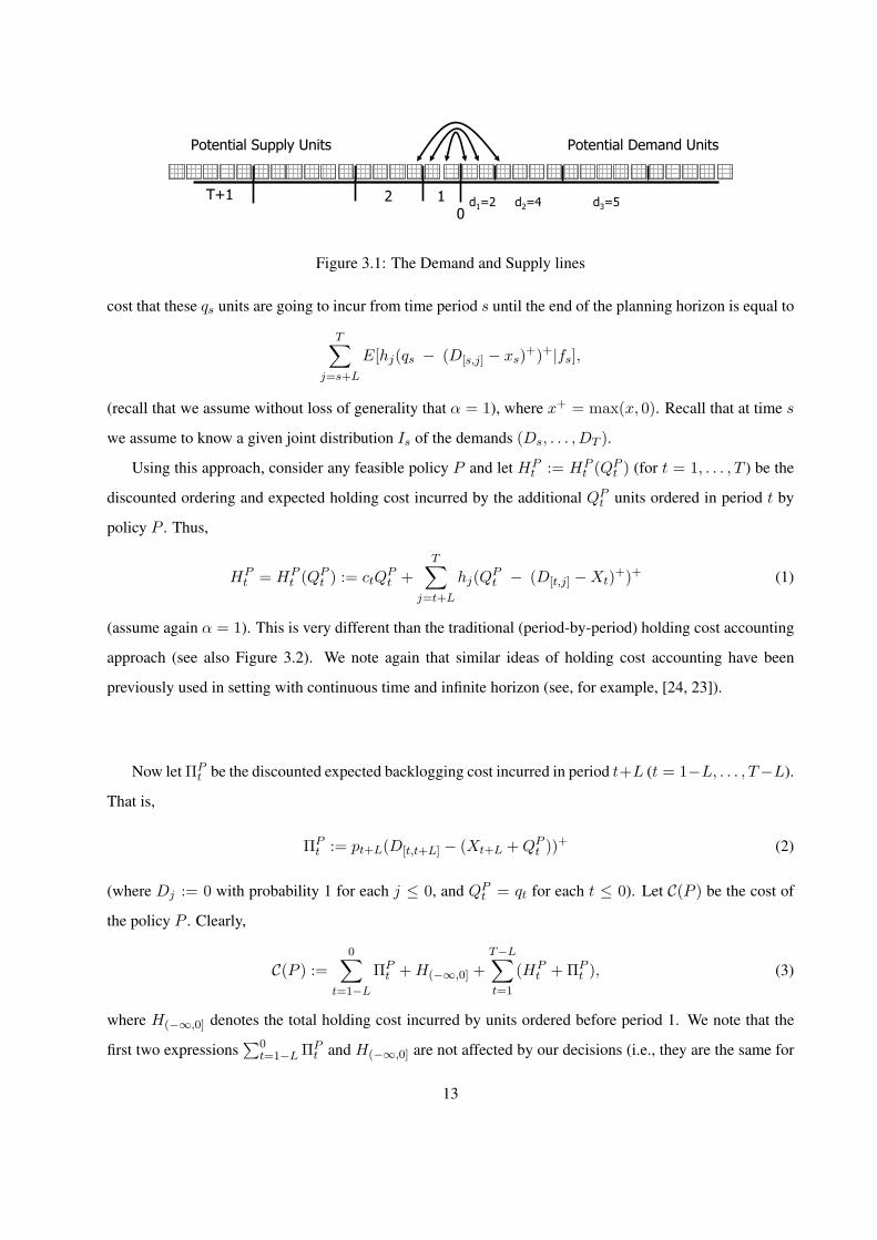
Figure 3.1: The Demand and Supply lines

cost that these qs units are going to incur from time period s until the end of the planning horizon is equal to

T∑

j=s+L

E[hj(qs − (D[s,j] − xs)+)+|fs],

(recall that we assume without loss of generality that α = 1), where x+ = max(x, 0). Recall that at time s

we assume to know a given joint distribution Is of the demands (Ds, . . . , DT ).

Using this approach, consider any feasible policy P and let HPt := HP

t (QPt ) (for t = 1, . . . , T ) be the

discounted ordering and expected holding cost incurred by the additional QPt units ordered in period t by

policy P . Thus,

HPt = HP

t (QPt ) := ctQ

Pt +

T∑

j=t+L

hj(QPt − (D[t,j] −Xt)+)+ (1)

(assume again α = 1). This is very different than the traditional (period-by-period) holding cost accounting

approach (see also Figure 3.2). We note again that similar ideas of holding cost accounting have been

previously used in setting with continuous time and infinite horizon (see, for example, [24, 23]).

Now let ΠPt be the discounted expected backlogging cost incurred in period t+L (t = 1−L, . . . , T−L).

That is,

ΠPt := pt+L(D[t,t+L] − (Xt+L + QP

t ))+ (2)

(where Dj := 0 with probability 1 for each j ≤ 0, and QPt = qt for each t ≤ 0). Let C(P ) be the cost of

the policy P . Clearly,

C(P ) :=0∑

t=1−L

ΠPt + H(−∞,0] +

T−L∑

t=1

(HPt + ΠP

t ), (3)

where H(−∞,0] denotes the total holding cost incurred by units ordered before period 1. We note that the

first two expressions∑0

t=1−L ΠPt and H(−∞,0] are not affected by our decisions (i.e., they are the same for

13

any feasible policy and each realization of the demand), and therefore we will omit them. Since they are

non-negative, this will not affect our approximation results. Also observe that without loss of generality, we

can assume that QPt = HP

t = 0 for any policy P and each period t = T − L + 1, . . . , T , since nothing that

is ordered in these periods can be used within the given planning horizon. We now can write

C(P ) =T−L∑

t=1

(HPt + ΠP

t ). (4)

The cost accounting scheme in (4) above is marginal, i.e., in each period we account all the expected costs

that become independent of any future decision (i.e., costs that become inevitable). In the next section, we

shall demonstrate that this new cost accounting approach serves as a powerful tool for designing simple

approximation algorithms that can be analyzed with respect to their worst-case expected performance.

4 Dual-Balancing Policy

In this section, we consider a new policy for the uncapacitated periodic-review stochastic inventory control

problem, which we call a dual-balancing policy. In this model the goal is to attempt and satisfy future

demands just on time. The key intuition is that since the exact future demands are not known (only their

distribution) any policy incurs two opposing expected costs. That is, each policy incurs an expected holding

cost resulting from over ordering and an expected backlogging cost resulting from under ordering. The

dual-balancing policy balances, in each period, the expected marginal holding cost against the expected

marginal backlogging penalty cost. In each period s = 1, . . . , T −L, we focus on the units that we order in

period s only, and balance the expected holding cost they are going to incur over [s, T ] against the expected

backlogging cost in period s + L. We do that using the marginal accounting of the holding cost that was

introduced in Section 3 above.

We next describe the details of the policy, which is very simple to implement, and then analyze its

expected performance. In particular, we will show that for any input of demand distributions and cost

parameters, the expected cost of the dual-balancing policy is at most twice the expected cost of an optimal

policy. We will then show that the worst-case guarantee of 2 is tight. Specifically, we will show that there

exists a set of instances for which the ratio between the expected cost of the dual-balancing policy and the

expected cost of the optimal policy converges to 2 asymptotically.

Recall the assumption discussed in Section 2 that the cost parameters imply no speculative motivation for

holding inventory or backorders. Using this assumption and a standard cost transformation from inventory

theory, we can assume, without loss of generality that ct = 0 and ht, pt ≥ 0, for each t = 1, . . . , T .

14

Moreover, we first describe the algorithm and its analysis under the latter assumption. Then in Sub-Section

4.5 we discuss in detail the generality of this assumption. In that sub-section, we will also show how a

simple cost transformation can yield a better worst-case performance guarantee and certainly a better typical

(average) performance in many cases in practice.

In the rest of the paper, we will use a superscripts B and OPT to refer to the dual-balancing policy

described below and an optimal policy, respectively.

4.1 The Algorithm

We first describe the algorithm and its analysis in the case where fractional orders are allowed. Later, we

will show how to extend the algorithm and the analysis to the case in which the demands and the order sizes

are integer-valued. In each period s = 1, . . . , T − L, we consider a given information set fs (where again

fs ∈ Fs) and the resulting pair (xBs , Is), where xB

s is the inventory position of the dual-balancing policy at

the beginning of period s and Is is the conditional joint distribution Is of the demands (Ds, . . . , DT ). We

then consider the following two functions:

(i) The expected holding cost over [s, T ] incurred by the additional qs units ordered in period s, condi-

tioned on fs. We denote this function by lBs (qs), where lBs (qs) := E[HBs (qs)|fs]. As we have seen in

Equation (1),

HBt (Qt) :=

T∑

j=t+L

hj(Qt − (D[t,j] −Xt)+)+

(recall that ct = 0).

(ii) The expected backlogging cost incurred in period s + L as a function of the additional qs units or-

dered in period s, conditioned again on fs. We denote this function by πBs (qs), where πB

s (qs) :=

E[ΠBs (qs)|fs]. In Equation (3) we have defined

ΠBt := pt(D[t,t+L] − (XB

t + Qt))+ = pt(D[t,t+L] − Y Bt )+.

We note that conditioned on a specific fs ∈ Fs and given any policy P , we already know xs, the

starting inventory position in time period s. Hence, the backlogging cost in period s, ΠBs |fs, is indeed

a function only of qs and future demands.

The dual-balancing policy now orders qBs = q′s units in period s, where q′s is such that lBs (q′s) = πB

s (q′s). In

other words, we set q′s so that the expected holding cost incurred over the time interval [s, T ] by the additional

q′s units we order at s is equal to the expected backlogging cost in period s + L, i.e., E[HBs (q′s)|fs] =

15

E[ΠBs (q′s)|fs]. Since we assume that fractional orders are allowed, we know that the functions lPt (qt) and

πPt (qt) are continuous in qt, for each t = 1, . . . , T − L and each feasible policy P .

Note again that for any given policy P , once we condition on a specific information set fs ∈ Fs, we

already know xPs deterministically. It is then straightforward to verify that both lPs (qs) and πP

s (qs) are

convex functions of qs. Moreover, the function lPs (qs) is equal to 0 for qs = 0 and is an increasing function

in qs, which goes to infinity as qs goes to infinity. In addition, the function πPs (qs) is non-negative for qs = 0

and is a decreasing function in qs, which goes to 0 as qs goes to infinity. Thus, q′s is well-defined and we can

indeed balance the two functions.

Observe the difference between the marginal holding cost function ls that accounts for costs over an

entire time interval, and the backlogging cost function πs that accounts for costs incurred in a single period.

The intuitive explanation is that in an uncapacitated model, under ordering (i.e., ordering ‘too little’) can

always be fixed in the next period to avoid further costs. On the other hand, since we can not order a negative

number of units, over ordering (i.e., ordering ‘too many’ units) can not be fixed by any decision made in

future periods, and the resulting costs are only a function of future demands, not of future orders. We also

point out that q′s can be computed as the minimizer of the function

gs(qBs ) := maxlBs (qs), πB

s (qs).

Since gs(qs) is the maximum of two convex functions of qs, it is also a convex function of qs. This implies

that in each period s we need to solve a single-variable convex minimization problem and this can be solved

efficiently given that the functions lBs and πBs can be evaluated efficiently. The complexity of the algorithm is

of order T (number of time periods) times the complexity of solving the single variable convex minimization

defined above. Note that q′s lies at the intersection of two monotone convex functions, which suggests that

bi-section methods can be effective in computing q′s.

In particular, the functions ls and πs consist of a sum of partial expectations. Observe that xs is known at

time s and these are expectations of simple piecewise linear functions. If the accumulated demand D[s,j] (for

each j ≥ s) has any of the distributions that are commonly used in inventory theory (e.g., Normal, Gamma,

Lognormal, Laplace, etc) [30], then it is extremely easy to evaluate the functions lPs (qs) and πPs (qs). If

the distribution of D[s,j] is discrete, these functions can be computed recursively in efficient ways using

the CDF functions. More generally, the complexity of evaluating the functions lPs (qs) and πPs (qs) and

minimizing gs(qs) can vary depending on the level of information we assume on the demand distributions

and their characteristics. In all of the common scenarios there exist straightforward methods to solve this

problem efficiently (see also [12] for a discussion on implementation issues and the performance of the dual-

16

balancing policy when demand follows an MMFE model). Note that in the presence of positive lead times

even computing a simple myopic policy requires the same knowledge on the distribution of the accumulated

demand over the lead time. Thus, it seems that the computational effort involved with implementing the

dual-balancing policy is of the same order of magnitude as the myopic policy.

Finally, observe that the dual-balancing policy is not a state-dependent base-stock policy. That is, the

control of the dual-balancing policy does depend on the inventory control policy in past periods, namely on

xBs . However, it can be implemented on-line, i.e., it does not require any knowledge of the control policy in

future periods. Thus, we avoid the burden of solving large dynamic programming problems. Moreover, un-

like the myopic policy, the dual-balancing policy is using in each period, available distributional information

about the future demands.

This concludes the description of the algorithm for the continuous-demand case. Next we describe the

analysis of the worst-case expected performance of this policy.

4.2 Analysis

Next we shall show that, for each instance of the problem, the expected cost of the dual-balancing policy

described above is at most twice the expected cost of an optimal policy. We will use the marginal cost

accounting approach described in Section 3 (see Equation (4) above), and amortize the period cost of the

dual-balancing policy with the cost of the optimal policy. That is, we will show that the optimal policy must

incur on expectation at least half of the period expected cost of the dual-balancing policy.

Using the marginal holding cost accounting approach discussed in Section 3, the expected cost of the

dual-balancing policy can be expressed as

E[C(B)] =T−L∑

t=1

E[HBt + ΠB

t ]. (5)

For each t = 1, . . . , T −L, let Zt be the random balanced cost by the dual-balancing policy in period t, i.e.,

Zt = E[HBt |Ft] = E[ΠB

t |Ft]. Note that Zt is realized in period t as a function of the observed information

set ft (we will denote its realization by zt). By the construction of the dual-balancing policy, we know that,

with probability 1, E[HBt |Ft] = E[ΠB

t |Ft], for each period t = 1, . . . , T − L. This implies that, for each

period t, E[HBt + ΠB

t |Ft] = 2Zt, which proves the following lemma follows.

Lemma 4.1 The expected cost of the dual-balancing policy is equal to twice the expected sum of the Zt

variables, i.e., E[C(B)] = 2∑T−L

t=1 E[Zt].

17

Proof : Using the marginal cost accounting scheme discussed in Section 3 and a standard argument of

conditional expectations we express

E[C(B)] =T−L∑

t=1

E[HBt + ΠB

t ] =T−L∑

t=1

E[E[HBt + ΠB

t |Ft]] = 2T−L∑

t=1

E[Zt].

Next we will state and prove two lemmas which imply that the expected cost of an optimal policy is at

least∑T−L

t=1 E[Zt]. For each realization of the demands D1, . . . , DT , let TH be the set of periods in which

the optimal policy had more inventory than the dual-balancing policy, i.e., the set of periods t such that

Y Bt < Y OPT

t . Let TΠ be the set of periods in which the dual-balancing had at least as much inventory as

OPT , i.e., the set of periods t such that Y Bt ≥ Y OPT

t . Observe that TH and TΠ are random sets that induce

a random partition of the planning horizon. The next lemma shows that, with probability 1, the marginal

holding cost incurred by the dual-balancing policy in periods t ∈ TH is at most the overall holding cost

incurred by OPT , denoted by HOPT , i.e.,∑

t∈THHB

t ≤ HOPT with probability 1.

Recall the concepts of LD, the line of potential units of demand to be realized over the horizon, and

LS , the line of supply units to be ordered over the planning horizon, discussed in Section 3 above. Since

the demand is independent from the inventory policy, we can compare between any two feasible policies by

looking at the respective periods in which each supply unit in LS was ordered. The proof technique in the

next lemma will be based on such comparison between the dual-balancing policy and an optimal policy

Lemma 4.2 For each realization fT ∈ FT , the marginal holding cost incurred by the dual-balancing

policy in all periods t ∈ TH is at most the overall holding cost incurred by OPT , denoted by HOPT , i.e.,∑

t∈THHB

t ≤ HOPT with probability 1.

Proof : Consider an information set fT ∈ FT which corresponds to a complete evolution over the planning

horizon, and some period s ∈ TH . We slightly abuse the notation and let TH denote the deterministic set of

periods that corresponds to the specific information set fT . Let Qs ⊆ LS be the set of supply units ordered

by the dual-balancing policy in period s, where clearly, |Qs| = q′s the balancing order quantity in period s.

By the definition of TH , we know that in period s we had yBs < yOPT

s . This implies that the units in Qs

were ordered by OPT either in period s or even prior to s. Since we assume that cs = 0 and that ht ≥ 0 for

each period t, we conclude that the holding cost that these units have incurred in OPT is at least as much

as the holding cost they have incurred in the dual-balancing policy.

We conclude the proof by observing that the sets Qs : s ∈ TH are of disjoint supply units since

they consist of units ordered by the dual-balancing policy in different periods. This implies that indeed

18

∑t∈TH

HBt ≤ HOPT , with probability 1.

The next lemma shows that, with probability 1, the marginal backlogging penalty cost of the dual-

balancing policy associated with periods t ∈ TΠ is at most the overall backlogging penalty incurred by

OPT , denoted by ΠOPT .

Lemma 4.3 For each realization fT ∈ FT , the marginal backlogging penalty cost of the dual-balancing

policy associated with all periods t ∈ TΠ is at most the overall backlogging penalty incurred by OPT ,

denoted by ΠOPT , i.e.,∑

t∈TΠΠB

t ≤ ΠOPT with probability 1.

Proof : Consider a realization fT ∈ FT and some period s ∈ TΠ (where again we abuse the notation and

use TΠ to denote a deterministic set). Note that period s is associated with the backlogging cost incurred in

period s + L. By definition of TΠ we know that yBs ≥ yOPT

s . However, this implies that, with probability 1,

the backlogging cost incurred by the dual-balancing policy in period s+L are no greater than the respective

backlogging cost incurred by the optimal policy in period s + L. The proof then follows.

As a corollary of Lemmas 4.1, 4.2 and 4.3 we get the following theorem.

Theorem 4.4 The dual-balancing policy for the uncapacitated periodic-review stochastic inventory control

problem has a worst-case performance guarantee of 2, i.e., for each instance of the problem, the expected

cost of the dual-balancing policy is at most twice the expected cost of an optimal solution, i.e.,

E[C(B)] ≤ 2E[C(OPT )].

Proof : From Lemma 4.1, we know that the expected cost of the dual-balancing policy is equal to twice the

expected cost of the sum of the Zt variables, i.e.,

E[C(B)] = 2T−L∑

t=1

E[Zt].

From Lemmas 4.2 and 4.3 we know that, with probability 1, the cost of OPT is at least as much as the

holding cost incurred by units ordered by the dual-balancing policy in periods t ∈ TH plus the backlogging

cost of the dual-balancing policy that is associated with periods t ∈ TΠ. In other words, with probability 1,

HOPT +ΠOPT ≥ ∑t∈TH

HBt +

∑t∈TΠ

ΠBt . Using again conditional expectations and the definition of Zt,

this implies that indeed,

19

E[C(OPT )] ≥ E[∑

t∈TH

HBt +

∑

t∈TΠ

ΠBt ] =

∑t

E[HBt · 11(t ∈ TH) + ΠB

t · 11(t ∈ TΠ)] =

∑t

E[E[HBt · 11(t ∈ TH) + ΠB

t · 11(t ∈ TΠ)|Ft]] =

∑t

E[(11(t ∈ TH) + 11(t ∈ TΠ))Zt] =∑

t

E[Zt].

We note that if the optimal policy is deterministic (i.e., it makes deterministic decisions in each period t

given the observed information set ft), then if we condition on Ft, yBt and yOPT

t are known deterministically,

and so are the indicators 11(t ∈ TH) and 11(t ∈ TΠ). Suppose that the optimal policy is a randomized policy,

i.e., it selects an order of size QOPTt as a random function of ft, then the same arguments above still work.

We now need to condition not only on Ft but also on QOPTt . Since the inventory control policy does not

have any effect on the evolution of the future demands, the arguments above are still valid. This concludes

the proof of the theorem.

4.3 Integer-Valued Demands

We now discuss the case in which the demands are integer-valued random variables, and the order in each

period is also restricted to an integer. In this case, in each period s, the functions lBs (qBs ) and πB

s (qBs )

are originally defined only for integer values of qBs . We define these functions for any value of qB

s by

interpolating piecewise linear extensions of the integer values. It is clear that these extended functions

preserve the properties of convexity and monotonicity discussed in the previous (continuous) case. However,

it is still possible (and even likely) that the value q′s that balances the functions lBs and πBs is not an integer.

Instead we consider the two consecutive integers q1s and q2

s := q1s + 1 such that q1

s < q′s < q2s . In particular,

q′s := λq1s + (1 − λ)q2

s for some 0 < λ < 1. In periods, we now order q1s units with probability λ and q2

s

units with probability 1− λ. This constructs what we call a randomized dual-balancing policy.

Observe that now at the beginning of time period s the order quantity of the dual-balancing policy is

still a random variable QBs = Q′

s with support consists of two points q1s , q

2s = q1

s(fs), q2s(fs) which

is a function of the observed information set fs. We would like to show that this policy admits the same

performance guarantee of 2. For each t = 1, . . . , T − L, let Zt be again the random balanced cost of

the dual-balancing policy in period t. Focus now on some period s. For a given observed information set

20

fs ∈ Fs we have for some 0 ≤ λ = λ(fs) ≤ 1,

zs = E[HBs (Q′

s)|fs] = λE[HBs (q1

s)|fs] + (1− λ)E[HBs (q2

s)|fs] =

E[HBs (λq1

s + (1− λ)q2s)|fs],

and

zs = E[πBs (Q′

s)|fs] = λE[πBs (q1

s)|fs] + (1− λ)E[πBs (q2

s)|fs] =

E[πBs (λq1

s + (1− λ)q2s)|fs].

The second equality (in each of the two expressions above) follows from the fact that we consider piecewise

linear functions. By the definition of the algorithm we also have

λE[HBs (q1

s)|fs] + (1− λ)E[HBs (q2

s)|fs] = λE[πBs (q1

s)|fs] + (1− λ)E[πBs (q2

s)|fs]. (6)

It is now readily seen that, for each period s and each fs ∈ Fs, we again have

E[HBs (Q′

s) + πBs (Q′

s)|fs] = 2zs, i.e., E[HBs (Q′

s) + πBs (Q′

s)|Fs] = 2Zs. This implies that Lemmas 4.1is

still valid.

Now define the sets TH and Tπ in the following way. Let TH = t : XBt + Q2

t ≤ Y OPTt , and

Tπ = t : XBt + Q2

t > Y OPTt . Observe that for each period s, conditioned on some fs ∈ Fs, we know

deterministically xBs , qB

2 and, if the optimal policy is deterministic, we also know yOPTs . Therefore, we

know whether s ∈ TH or s ∈ TΠ. If the optimal policy is also a randomized policy, we condition not

only on fs but also on the decision made by the optimal policy in period s. Moreover, if s ∈ TH , then,

with probability 1, Y Bs ≤ Y OPT

s , and if s ∈ Tπ, then, with probability 1, Y Bs ≥ Y OPT

s . This implies that

Lemmas 4.2 and 4.3 are also still valid. The following theorem is now established (the proof is identical to

that of Theorem 4.4 above).

Theorem 4.5 The randomized dual-balancing policy has a worst-case performance guarantee of 2, i.e.,

for each instance of the uncapacitated periodic-review stochastic inventory control problem, the expected

cost of the randomized dual-balancing policy is at most twice the expected cost of an optimal solution, i.e,

E[C(B)] ≤ 2E[C(OPT )].

4.3.1 Dual-Balancing - Bad Example

We shall show that the above analysis is tight. Consider an instance with h > 0, p = h√

L where L > 0

is again the a positive integer that denotes the lead time between the time an order is placed and the time it

21

arrives. Also assume that T = 1+2L and α = 1. The random demands have the following structure. There

is one unit of demand that is going to occur with equal probability either in period L+1 or in period 2L+1.

For each t 6= L + 1, 2L + 1, we have Dt = 0 with probability 1. Fractional orders are allowed.

It is readily verified that the optimal policy orders 1 unit in period 1 and incurs expected cost of 12hL.

On the other hand, the dual-balancing policy will order in each one of the periods 1, . . . ,√

L + 1 just a

small amount of the commodity. In particular, in period 1, the dual-balancing orders 1√L+1

of a unit (this

can be calculated by equating 12(√

Lh)(1 − q) = 12Lhq, where q is the size of the order). It can be easily

verified that when L goes to ∞, the ratio between the expected cost of the dual-balancing policy and the

expected cost of the optimal policy converges to 2 (the calculations are rather messy to present but can be

easily coded).

4.4 Stochastic Lead Times

Next, we consider the more general model, where the lead time of an order placed in period s is some

integer-valued random variable Ls (here we deviate from our convention in that ls is not he realization of Ls

but the function defined above). However, we assume that the random variables L1, . . . , LT are correlated,

and in particular, that s + Ls ≤ t + Lt for each s ≤ t. In other words, we assume that any order placed at

time s will arrive no later than any other order placed after period s. This is a very common assumption in

the inventory literature, usually described as ”no order crossing”.

We next describe a version of the dual-balancing that provides a 2-approximation algorithm for this

more general model. LetAs be the set of all periods t ≥ s such that an order placed in s is the latest order to

arrive by time period t. More precisely, As := t ≥ s : s + Ls ≤ t and t′ + Lt′ > t, ∀t′ ∈ (s, t]. Clearly,

As is a random set of demands. Observe that the sets AsTs=1 induce a partition of the planning horizon.

Hence, we can write the cost of each feasible policy P in the following way:

C(P ) =T∑

s=1

(HPs + (

∑

t∈As

ΠPt ))

Now let ΠPs :=

∑t∈As

ΠPt and write C(P ) =

∑Ts=1(H

Ps + ΠP

s ). Similar to the previous case, we

consider in each period s the two functions E[HBs |fs] and E[ΠB

s |fs], where again fs is the information set

observed in period s. Here the expectation is with respect to future demands as well as future lead times.

Finally we order qBs units to balance these two functions. By arguments identical to those in Lemmas 4.1,

4.2 and 4.3 we conclude that this policy yields a worst-case performance guarantee of 2.

22

Observe that in order to implement the dual-balancing policy in this case, we have to know in period s

the conditional distributions of the lead times of future orders (as seen from period s conditioned on some

fs ∈ Fs). This is required in order to evaluate the function E[ΠBs |fs].

4.5 Cost Transformation

In this section, we discuss in detail the cost transformation that enables us to assume, without loss of gen-

erality that, for each period t = 1, . . . , T , we have ct = 0 and ht, pt ≥ 0. Consider any instance of

the problem with cost parameters that imply no speculative motivation for holding inventory or backorders

(as discussed in Section 2). We use a simple standard transformation of the cost parameters (see [30]) to

construct an equivalent instance, with the property that for each period t = 1, . . . , T , we have ct = 0 and

ht, pt ≥ 0. The modified instance has the same set of optimal policies. Applying the dual-balancing policy

to that instance will provide a policy that is feasible and also has a performance guarantee of at most 2 with

respect to the original problem. We shall also show that this cost transformation can improve the perfor-

mance guarantee of the dual-balancing policy in cases where the ordering cost is the dominant part of the

overall cost. In practice this is often the case.

We now describe the transformation for the case with no lead time (L = 0) and α = 1; the extension to

the case of arbitrary lead time and α < 1 is straightforward. Recall that any feasible policy P satisfies, for

each t = 1, . . . , T , Qt = NIt −NIt−1 + Dt (for ease of notation we omit the superscript P ). Using these

equations we can express the ordering cost in each period t as ct(NIt − NIt−1 + Dt). Now replace NIt

with NI+t −NI−t , its respective positive and negative parts.

This leads to the following transformation of cost parameters. We let ct := 0, ht := ht + ct −ct+1 (cT+1 = 0) and pt := pt − ct + ct+1. Note that the assumptions on the cost parameters ct, ht,

and pt discussed in Section 2, and in particular, the assumption that there is no speculative motivation for

holding inventory or backorders, imply that ht and bt above are non-negative (t = 1, . . . , T ). Observe that

the parameters ht and bt will still be non-negative even if the parameters ct, ht, and pt are negative and as

long and the above assumption holds. Moreover, this enables us to incorporate into the model a negative

salvage cost at the end of the planning horizon (after the cost transformation we will have non-negative

cost parameters). It is readily verified that the induced problem is equivalent to the original one. More

specifically, for each realization of the demands, the cost of each feasible policy P in the modified input

decreases by exactly∑T

t=1 ctdt (compared to its cost in the original input). Therefore, any optimal policy

for the modified input is also optimal for the original input.

Now apply the dual-balancing policy to the modified problem. We have seen that the assumptions

23

on ct, ht and pt ensure that ht and pt are non-negative and hence the analysis presented above is valid.

Let opt and ¯opt be the optimal expected cost of the original and modified inputs, respectively. Clearly,

opt = ¯opt + E[∑T

t=1 ctDt]. Now the expected cost of the dual-balancing policy in the modified input is at

most 2 ¯opt. Its cost in the original input is then at most 2 ¯opt+E[∑T

t=1 ctDt] = 2opt−E[∑T

t=1 ctDt]. This

implies that if E[∑T

t=1 ctDt] is a large fraction of opt, then the performance guarantee of the expected cost of

the dual-balancing policy might be significantly better than 2. For example, in case E[∑T

t=1 ctDt] ≥ 0.5opt

we can conclude that the expected cost of the dual-balancing policy would be at most 1.5opt. It is indeed the

case in some real life problems that a major fraction of the total cost is due the ordering cost. The intuition

of the above transformation is that∑T

t=1 ctDt is a cost that any feasible policy must pay. As a result, we

treat it as an invariant in the cost of any policy and apply the approximation algorithm to the rest of the cost.

In the case where we have a lead time L, we use the equations Qt := NIt+L −NIt+L−1 + Dt+L, for

each t = 1, . . . , T − L, to get the same cost transformation. The transformation for α > 1 is also straight

forward.

5 A Class of Myopic Policies

For many periodic-review inventory control problems with inter-temporal correlated demands, there is no

known computationally tractable procedure for finding the optimal base-stock inventory levels. As a result,

various simpler heuristics have been considered in the literature. In particular, many researchers have con-

sidered a myopic policy. In the myopic policy, we follow a base-stock policy Rmy(ft) : ft ∈ Ft. For

each period t and possible information set in period t, the target inventory level Rmy(ft) is computed as

the minimizer of a one-period problem. More specifically, in period s = 1, . . . , T − L we focus only on

minimizing the expected immediate cost that is going to be incurred in this period (or in s + L in the pres-

ence of a lead time L). In other words, the target inventory level Rmy(fs) minimizes the expected holding

and backlogging costs in period s + L, while ignoring the cost over the rest of the horizon (i.e., the cost

over (s + L, T + 1]). This optimization problem has been proven to be convex and hence easy to solve (see

[30]). It is then possible to implement the myopic policy on-line, where in each period s, we compute the

base-stock level based on the current observed information set fs. For each period t and each ft ∈ Ft, the

myopic base-stock level provides an upper bound on the optimal base-stock level (see [30] for a proof). The

intuition is that the myopic policy underestimates the holding cost, since it considers only the one-period

holding cost. Therefore, it always orders more units than the optimal policy. Clearly, this policy might

not be optimal in general, though in many cases it seems to perform extremely well. Under rather strong

24

conditions it might even be optimal (see [29, 10, 11, 17]). A natural question to ask is whether the myopic

policy yields a constant performance guarantee for the periodic-review inventory control problem, i.e., is its

expected cost always bounded by some constant times the optimal expected cost.

In this section, we provide a negative answer to this question. We show that the expected cost of the

myopic policy can be arbitrarily more expensive than the expected optimal cost, even for the case when the

demands are independent and the costs are stationary. The example that we construct provides important

intuition concerning the cases for which the myopic policy performs poorly. In addition, we describe an

extended class of myopic policies that generalizes the myopic policy discussed above. It is interesting that

this class of policies also provides a lower bound on the optimal base-stock levels.

5.1 Myopic Policy - Bad example

Consider the following set of instances parameterized by T , the number of periods. We have a per-unit

ordering cost of c = 0, a per-unit holding cost h = 1 and a unit backlogging penalty p = 2. The demands are

specified as follows, D1 ∈ 0, 1 with probability 0.5 for 0 and 1, respectively. For t = 2, . . . , T −1, Dt :=

0 with probability 1, and DT := 1 with probability 1. The lead time is considered to be equal 0, and α = 1.

It is easy to verify that the myopic policy will order 1 unit in period 1 and that this will result an expected

cost of 0.5T . On the other hand, if we do not order in period 1, then the expected cost is 1. This implies that

as T becomes larger the expected cost of the myopic policy is Ω(T ) times as expensive as the expected cost

of the optimal policy.

The above example indicates that the myopic policy may perform poorly in cases where the demand

from period to period can vary a lot, and forecasts can go down. There are indeed many real-life situations,

when this is exactly the case, including new markets, volatile markets or end-of-life products.

5.2 A Class of Myopic Policies

As we mentioned before, by considering only the one-period problem, the myopic policy described above

underestimates the actual holding cost that each unit ordered in period t is going to incur. This results in

base-stock levels that are higher than the optimal base-stock levels.

We now describe an alternative myopic base-stock policy that we call a minimizing policy. We shall

show that the base-stock levels of this policy are always smaller than the corresponding optimal base-stock

levels. Thus, combined with the classical myopic base-stock levels we derive both lower and upper bounds

on the optimal base-stock levels. These bounds can be used in computing good inventory control policies.

In particular, in follow-up work, Hurley, Jackson, Levi, Roundy and Shmoys [?] have shown that they these

25

bounds can be used to derive improved balancing policy. These policies have a worst-case guarantee of 2

and their typical performance is significantly better than the dual-balancing policy described in this paper.

In addition, they have shown that each policy that deviates from these respective lower and upper bounds

can be improved.

Recall the functions lPs (qs), πPs (qs) defined in Section 4 for each period s = 1, . . . , T−L, where qs ≥ 0.

Since at each period s we know xs, we can equivalently write lPs (ys−xs), πPs (ys−xs), where ys ≥ xs. We

now consider in each period s the problem: minimize (lPs (ys− xs) + πPs (ys−xs)) subject to ys ≥ xs , i.e.,

minimize the expected ordering and holding costs incurred by the units ordered in period s over [s, T ] and

the backlogging cost incurred in period s+L, conditioned on some fs ∈ Fs. We have already seen that this

function is convex in ys. Observe that lPs (ys−xs)− lPs (ys) and πPs (ys−xs)−πP

s (ys) do not depend on ys

for ys ≥ xs. This gives rise to the following equivalent one-period problem: minys≥xs(lPs (ys) + πPs (ys)).

That is, both problems have the same minimizer. It is also clear that the new minimization problem is also

convex in ys and is easy to solve, in many cases as easy as the one-period problem solved by the myopic

policy described above. We note that the function we minimize was used by Chan and Muckstadt [2].

For each t = 1, . . . , T and ft ∈ Ft, let RM (ft) be the smallest base-stock level resulted from the

minimizing policy in period t, for a given observed information set ft. We now show that for each period t

and ft ∈ Ft, we have RM (ft) ≤ ROPT (ft), where ROPT (ft) is the optimal base-stock level.

Theorem 5.1 For each period t and ft ∈ Ft, we have RM (ft) ≤ ROPT (ft).

Proof : Recall the dynamic programming based framework described in Section 3. Observe that for each

state (xt, ft), we know that ROPT (ft) is the optimal base-stock level that results from the optimal solution

for the corresponding subproblem defined over the interval [t, T ]. It is enough to show that the optimal

solution for each such problem must be at least RM (ft).

Assume otherwise, i.e., ROPT (fs) < RM (fs) for some period s and for all optimal policies. Con-

sider now the base-stock policy P with base-stock level RP (fs) = RM (fs) for period s, and RP (ft) :=

ROPT (ft) for each t = s+1, . . . , T and ft ∈ Ft. We will show that P , starting from period s with observed

information set fs, has an expected cost that is smaller than the expected cost of the optimal solution. From

Section 3 we know that the expected cost of each policy P can be expressed as∑T−L

t=s E[HPt + ΠP

t ]. Now

by the definition of RM (fs) we know that

E[(HPs + ΠP

s )|fs] < E[(HOPTs + ΠOPT

s )|fs].

Moreover, for each t ∈ (s, T ], the inventory position Y Pt will always be at least Y OPT

t , and therefore

E[ΠPt |fs] ≤ E[ΠOPT

t |fs]. It is also clear that in each period t ∈ (s, T ], the QPt units ordered by policy

26

P in period t will always be a subset of the units ordered by OPT in this period. Therefore, for each

t = s + 1, . . . , T , we have that E[HPt |fs] ≤ E[HOPT

t |fs]. This concludes the proof.

We now define a generalization that captures the myopic policy and the minimization policy as two

special cases. For each t = 1, . . . , T − L, we define a sequence of one-period problems for each kt =

0, . . . , T − t, each generates a corresponding base-stock level. Given k, we define the one-period problem

that aims to minimize the expected ordering and holding cost incurred by the units ordered in period t over

the interval [t, t + L + kt], and the expected backlogging cost in period t + L. In other words, the parameter

kt defines the length of the horizon considered in the one-period problem being solved in period t. For each

sequence of k1, . . . , kT , we get a corresponding k-minimizing policy. It is clear that if kt = 0 for each t,

we get the myopic policy and if kt = T − t we get the minimizing policy. Note again that the myopic and

the minimizing policies provide an upper bound and lower bound, respectively, on the optimal base-stock

levels. We again refer to [?] for discussion on the performance of these policies.

6 The Stochastic Lot-Sizing Problem

In this section, we change the previous model and in addition to the per-unit ordering cost, consider a fixed

ordering cost K that is incurred in each period t with positive order (i.e., when Qt > 0). For ease of notation,

we will assume again, without loss of generality, that ct = 0. We call this model the stochastic lot-sizing

problem. The goal is again to find a policy that minimizes the expected discounted overall ordering, holding

and backlogging costs. Naturally, this model is more complicated. Here we will assume that L = 0, α = 1

and that in each period t = 1, . . . , T , the conditional joint distribution It of (Dt, . . . , DT ) is such that the

demand Dt is known deterministically (i.e., with probability 1). The underlying assumption here is that at

the beginning of period t our forecast for the demand in that period is sufficiently accurate, so that we can

assume it is given deterministically. A primary example is make-to-order systems.

As noted in Section 1, for many settings it is known that the optimal solution can be described as a set

(st, St) = (st(ft), St(ft))t. In each period t place an order if and only if the current inventory level is

below st. If we place an order in period t, we will increase the inventory level up to St. We next describe

a policy which we call the triple-balancing policy denoted by TB, and analyze its worst-case expected

performance. Specifically, we show that its expected cost is at most 3 times the expected cost of an optimal

policy. We note that in this case the policy and its analysis are identical for discrete and continuous demands.

27

6.1 The Triple-Balancing Policy

The policy follows two rules that specify when to place an order and how many units to order once an order

is placed:

Rule 1: When to order. At the beginning of period s, we let s∗ be the period in which the triple-balancing

policy has last placed an order, i.e., s∗ is the latest order placed so far. Thus, s∗ < s, where s∗ = 0 if no

order has been placed yet. We place an order in period s if and only if, by not placing it in period s, the

accumulated backlogging cost over the interval (s∗, s] exceeds K. If we place an order, we update s∗ and

set it equal to s. Observe that since, in each period s, the conditional joint distribution Is is such that Ds is

known deterministically, this procedure is well-defined.

Rule 2: How much to order If we place an order in period s < T , then we focus on the holding cost incurred

by the units ordered in s over the interval [s, T ], again using marginal cost accounting. We then order qBs

units such that

qBs := maxqs : E[HB

s (qs)|fs] ≤ K, where again fs ∈ Fs is the current information set. That is, we order

the maximum number of units as long as the conditional expectation of the holding cost that these units will

incur over [s, T ], as seen from time period s, is at most K. In case s = T , we just order enough to cover

all current back orders and the demand dT . Observe that qBs must always be large enough to cover all of

the backlogged units of demand over (s∗, s]. Hence, at the end of a period s in which an order was placed,

there are no unsatisfied units of demand. We note that since for each fs ∈ Fs, the function E[HBs (qs)|fs] is

convex in qs, it is relatively easy to compute qBs .

This concludes the description of the algorithm. Next we describe the analysis of the worst-case expected

performance.

6.2 Analysis

Let N be the random variable of the number of orders placed by the triple-balancing policy. We next define

a sequence of random variables S0, . . . , ST+1. We let S0 = 0, ST+1 = T + 1, and let Si (for i = 1, . . . , T )

be the time period in which the ith order of the triple-balancing policy was placed, or T + 1 if N < i

(i.e., the triple-balancing policy has placed fewer than i orders). Now, for each i = 0, . . . , T , let Zi be the

following random variable. If Si < T , then Zi is equal to the holding cost that the triple balancing policy

incurs over [Si, Si+1) (denoted by Hi) plus the backlogging and ordering costs it incurs over (Si, Si+1].

If Si ≥ T , then Zi = 0. Observe that [Si, Si+1) and [(Si, Si+1] are random intervals induced by the

triple-balancing policy. Similarly, we define the set of variables Z ′0, . . . , Z′T+1 with respect to the cost of

28

OPT over the corresponding intervals induced by the orders of the triple-balancing policy. It is clear that

C(B) =∑T

i=0 Zi · 11(Si < T ) and C(OPT ) =∑T

i=0 Z ′i · 11(Si < T ). We first develop a lower bound on

the expected cost of OPT using the expectation of the random variable N .

Lemma 6.1 For each instance of the stochastic lot-sizing problem with correlated demand the expected cost

of an optimal policy OPT is at least KE[N ].

Proof : We have already observed that C(OPT ) =∑T

i=0 Z ′i · 11(Si < T ). Using again the linearity of

expectation and conditional expectation, we can write,

E[C(OPT )] =T∑

i=0

E[11(Si < T )E[Z ′i|Si, FSi ]] ≥

T∑

i=0

E[11(Si < T )E[Z ′i · 11(Si+1 ≤ T )|Si, FSi ]]

Next we show that for each i = 0, . . . , T , we have that,

E[Z ′i · 11(Si+1 ≤ T )|Si, FSi ] ≥ K · Pr(Si+1 ≤ T |Si, FSi)

Conditioned on some Si = si and fsi ∈ Fsi , we know dsi (where si is the realization of Si). As a

result, we also know the inventory levels of OPT and the triple-balancing policy at the end of period si

deterministically. Therefore, exactly one of the following 2 cases must apply:

Case 1: At the end of period si, the inventory level of OPT is at most the inventory level of the triple-

balancing policy, i.e., yOPTsi

≤ yTBsi

. Now either OPT places an order over (si, Si+1] and hence incurs a

cost of at least K over this interval, or it does not; then, unless si is the last order of the triple-balancing

policy, it will incur backlogging cost of at least K.

Case 2: At the end of period si, the inventory level of OPT is strictly larger than the inventory level of the

triple-balancing policy, i.e., yOPTsi

> yTBsi

. However, by the construction of the triple-balancing policy, we

know that if OPT has more physical inventory, then the expected holding cost it will incur over [si, Si+1)

is at least K.

We conclude that in both cases, Z ′i·11(Si+1 ≤ T )|si, fsi)] ≥ K ·11(Si+1 ≤ T |si, fsi). Taking expectation

we have E[Z ′i · 11(Si+1 ≤ T )|Si, FSi ] ≥ K · Pr(Si+1 ≤ T |Si, FSi).

This implies that

E[C(OPT )] ≥ K · E[T∑

i=0

11(Si < T ) · Pr(Si+1 ≤ T |Si, FSi)] =

K · E[T∑

i=0

E[11(Si < T ) · 11(Si+1 ≤ T )|Si, FSi ]] = K · E[N ].

29

To finish the analysis we next show that the expected difference between the cost of the triple-balancing

policy (denoted by TB) and the cost of the optimal policy is at most 2KE[N ].

Lemma 6.2 For each instance of the problem, we have E[C(TB)− C(OPT )] ≤ 2KE[N ].

Proof : Clearly,

E[C(TB)− C(OPT )] = E[T∑

i=0

(Zi − Z ′i) · 11(Si < T )] =

T∑

i=0

E[11(Si < T ) · E[(Zi − Z ′i)|Si, FSi ]].

We next bound E[(Zi − Z ′i)|Si, FSi ] for each i = 0, . . . , T . For i = 0, it is clear that the holding costs

that the TB policy and OPT incur over [s0, S1) are identical (this cost is due initial inventory that exists

at the beginning of the horizon). Also observe that the backlogging and ordering costs of the TB policy

over (S0, S1] are at most K if S1 = T + 1 and at most 2K otherwise. In the latter case, we conclude that

OPT either placed an order on the interval (S0, S1] or incurred backlogging cost of at least K. Hence,

Z0 − Z ′0 ≤ K.

For each i = 1, . . . , T , we condition on some si and fsi ∈ Fsi . We then know what are yTBsi

and yOPTsi

deterministically. We now claim that:

(Zi − Z ′i)|si, fsi ≤ 11(yTBsi

≤ yOPTsi

) · (K + 11(Si+1 ≤ T |si, fsi) ·K) +

11(yTBsi

> yOPTsi

) · (Hi|si, fsi + 11(Si+1 ≤ T |si, fsi) ·K).

In first case where yTBsi

≤ yOPTsi

we know that OPT will incur over [si, Si+1) at least as much holding

cost as the TB policy. By the construction of the algorithm we know that the TB policy will not incur

more than K backlogging cost and will place at most one order over (si, Si+1]. In the second case where

yTBsi

> yOPTsi

we know that the ordering cost and backlogging costs of OPT over (si, Si+1] are at least K,

which is more than the backlogging cost the TB policy incurs on that interval. In addition, TB will incur

holding cost Hi|si, fsi over [si, Si+1) and will place at most one order over (si, Si+1]. Taking expectation

of both sides we conclude that:

E[(Zi − Z ′i)|Si, FSi ] ≤ E[11(yTBsi

≤ yOPTSi

) · (K + 11(Si+1 ≤ T ) ·K)|Si, Fsi ] +

E[11(yTBSi

> yOPTSi

) · (Hi + 11(Si+1 ≤ T ) ·K)|Si, FSi ] ≤ E[K + 11(Si+1 ≤ T )|Si, FSi ].

30

The last inequality is by the construction of the algorithm (E[Hi|si, fsi ] ≤ K] for each Si = si and

fsi ∈ Fsi). This implies that for each i = 2, . . . , T , we have

E[(Zi − Z ′i) · 11(Si < T )] = E[11(Si < T ) · E[Zi − Z ′i|Si,FSi ]] ≤

E[K + 11(Si+1 ≤ T )].

Finally, we have that:

E[T∑

i=0

(Zi − Z ′i) · 11(Si < T )] ≤

K + K · E[T∑

i=1

11(Si < T )] + K · E[T+1∑

i=1

11(Si < T ) · 11(Si+1 ≤ T )] =

K + K · E[N ] + K · (E[N ]− 1) = 2KE[N ].

As a corollary of Lemmas 6.1 and 6.2, we get the following theorem.

Theorem 6.3 For each instance of the stochastic lot-sizing problem, the expected cost of the triple-balancing

policy is at most 3 times the expected cost of an optimal policy.

7 Conclusions

In this paper we have proposed a new approach for devising provably good policies for stochastic inventory

control models with time dependent and correlated demand. These models are known to be hard, in the

sense that computing optimal policies is usually intractable. In turn our approach leads to policies that are

simple computationally and conceptually and provides constant performance guarantees on the worst-case

expected behavior of these policies.

We note that all of the results described in the paper can be extended under rather mild conditions to the

counterpart models with infinite horizon, where the goal is to minimize the expected average or discounted

cost. Specifically, it is sufficient to have an efficient oracle that can compute the functions ls and πs.

In a subsequent papers [16, 15], we consider two generalizations of the model considered in this paper:

the extension to the case where there exists a hard capacity constrain on the amount of units ordered in each

period, and the extension to multi-echelon supply chains. We use and extend some of the ideas introduced

in this paper to construct policies that provide worst-case performance guarantees. We think it would be an

interesting challenge to extend the ideas introduced in this paper to additional supply chain related models.

31

It would also be important to establish a more rigorous analysis of the computational hardness of these

models. As far as we know there does not exist any rigorous proof of that kind.

Acknowledgments We thank Shane Henderson for stimulating discussions and helpful suggestions

that made the paper significantly better.

We thank Jack Muckstadt for his valuable comments that lead to the extension to the stochastic lead times.

We thank the anonymous referees for numerous valuable comments that made the paper more precise and

improved it exposition. We specifically thank the anonymous referee who suggested the bad example dis-

cussed in Section 4.

References

[1] D. Bertsimas and A. Thiele. A robust optimization approach to supply chain management. In Pro-

ceedings of 14th IPCO, pages 86–100, 2004.

[2] E. W. M. Chan. Markov Chain Models for multi-echelon supply chains. PhD thesis, School of OR&IE,

Cornell University, Ithaca, NY, January 1999.

[3] M. Charikar, C. Chekuri, and M. Pal. Sampling bounds for stochastic optimization. Unpublished

manuscript, 2005.

[4] F. Chen and J. Song. Optimal policies for multi-echelon inventory problems with Markov-modulated

demand. Operations Research, 49:226–234, 2001.

[5] B. C. Dean, M. X. Goemans, and J. Vondak. Approximating the stochastic knapsack problem: The

benefit of adaptivity. In Proceedings of the 45th Annual IEEE Symposium on the Foundations of

Computer Science, 2004., pages 208–217, 2004.

[6] L. Dong and H. L. Lee. Optimal policies and approximations for a serial multiechelon inventory system

with time-correlated demand. Operations Research, 51, 2003.

[7] S. Dye, L. Stougie, and A. Tomasgard. The stochastic single resource service provision problem. Naval

Research Logistics, 50:869–887, 2003.

32

[8] N. Erkip, W. H. Hausman, and S. Nahmias. Optimal centralized ordering policies in multi-echelon

inventory systems with correlated demands. Mangement Science, 36:381–392, 1990.

[9] G. Gallego and O. Ozer. Integrating replenishment decisions with advanced demand information.

Management Science, 47:1344–1360, 2001.

[10] E. Ignall and A. F. Venott. Optimality of myopic inventory policies for several substitute products.

Managment Science, 15:284–304, 1969.

[11] T. Iida and P. Zipkin. Approximate solutions of a dynamic forecast-inventory model. Working paper,

2001.

[12] P. Jackson, G. Hurley, R. Levi, R. O. Roundy, and D. B. Shmoys. A computaqtional and theoreticla

study of stochatic inventory control policies in the MMFE model. In preparation, 2005.

[13] D. Joneja. The joint replenishment problem: new heuristics and worst case performance bounds.

Operations Research, 38:723–771, 1990.

[14] H. L. Lee, K. C. So, and C. S. Tang. The value of information sharing in two-level supply chains.

Mangement Science, 46:626–643, 1999.

[15] R. Levi, R. O. Roundy, D. B., and V. A. Troung. Provably near-optimal balancing policies for multi-

echelon stochastic inventory control models. Working paper, 2005.

[16] R. Levi, R. O. Roundy, D. B. Shmoys, and V. A. Troung. Approximation algorithms for capacitated

stochastic inventory control models. submitted, 2004.

[17] X. Lu, J. S. Song, and A. C. Regan. Inventory planning with forecast updates: approximate solutions

and cost error bounds. Working paper, 2003.

[18] R. H. Mohring, F. J. Radermacher, and G. Weiss. Stochastic scheduling problems I: general strategies.

ZOR- Zeitschrift fur Operations Research, 28:193–260, 1984.

[19] R. H. Mohring, F. J. Radermacher, and G. Weiss. Stochastic scheduling problems II: set strategies.

ZOR- Zeitschrift fur Operations Research, 29:65–104, 1984.

[20] R. H. Mohring, A. Schulz, and M. Uetz. Approximation in stochastic scheduling: the power of LP-

based priority policies. Journal of the ACM (JACM), 46:924–942, 1999.

33

[21] A. Muharremoglu and J. N. Tsitsiklis. A single-unit decomposition approach to multi-echelon inven-

tory systems. Working paper, 2001.

[22] O. Ozer and G. Gallego. Integrating replenishment decisions with advance demand information. Man-

agment Science, 47:1344–1360, 2001.

[23] S. Axsater. Simple solution procedures for a class of two-echelon inventory problems. Operations

Research, 38:64–69, 1990.

[24] S. Axsater and P. Lundell. In process safety stock. In Proceedings of the 23rd IEEE Conference on

Decision and Control, pages 839–842, 1984.

[25] D. B. Shmoys and C. Swamy. Stochastic optimization is (almost) as easy as deterministic optimization.

In Proceedings of the 45th Annual IEEE Symposium on the Foundations of Computer Science, 2004.,

pages 228–237, 2004.

[26] E. A. Silver and H. C. Meal. A heuristic selecting lot-size requirements for the case of a deterministic

time varying demand rate and discrete opportunities for replenishment. Production and Inventory

Management, 14:64–74, 1973.

[27] J. Song and P. Zipkin. Inventory control in a fluctuating demand environment. Operations Research,

41:351–370, 1993.

[28] L. Stougie and M. H. van der Vlerk. Approximation in stochastic integer programming. Technical

Report SOM Research Report 03A14, Eindhoven University of Technology, 2003.

[29] A. F. Veinott. Optimal policy for a multi-product, dynamic, non-stationary inventory problem. Man-

agement Science, 12:206–222, 1965.

[30] P. H. Zipkin. Foundation of inventory management. The McGraw-Hill Companies, Inc, 2000.

34

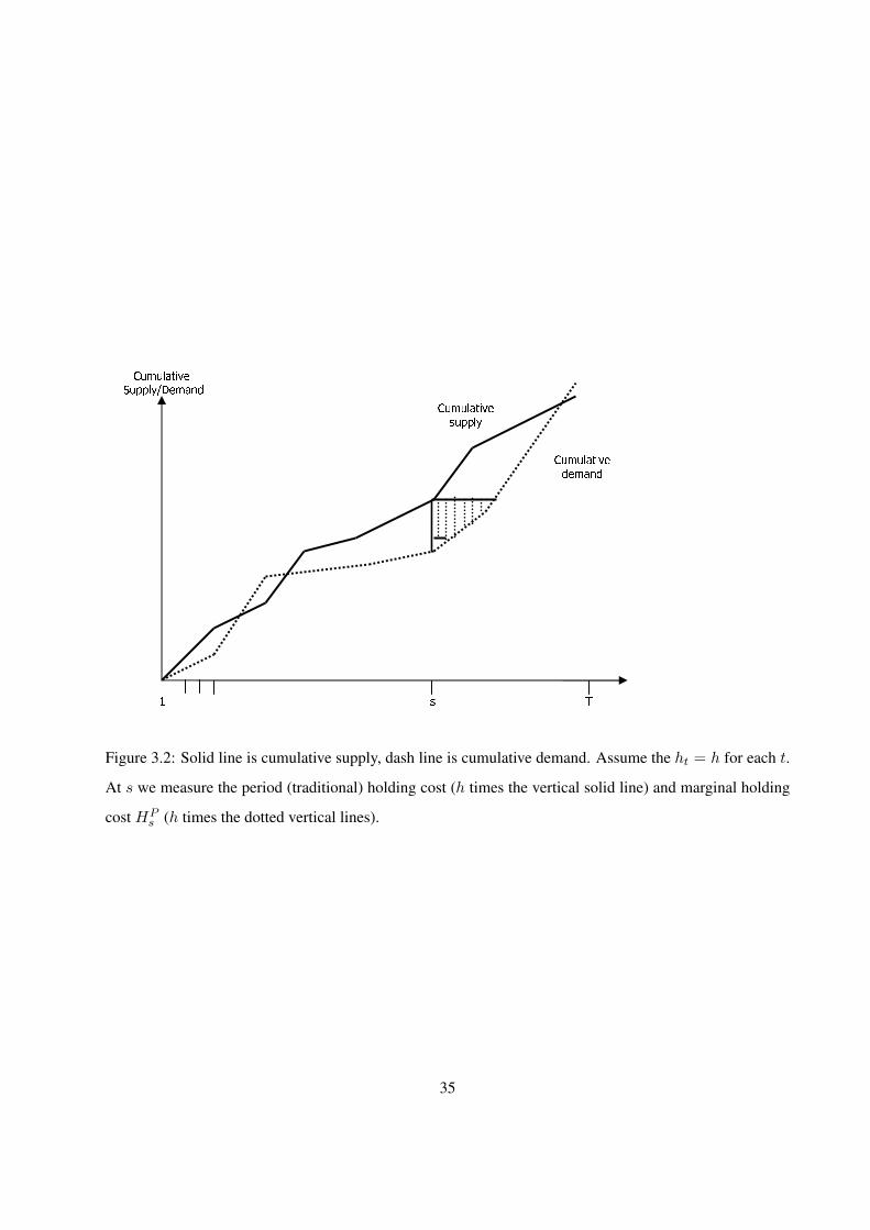
Figure 3.2: Solid line is cumulative supply, dash line is cumulative demand. Assume the ht = h for each t.

At s we measure the period (traditional) holding cost (h times the vertical solid line) and marginal holding

cost HPs (h times the dotted vertical lines).

35