Embed Size (px)
Citation preview
Submitted to Operations Research
manuscript OPRE-2009-06-260.R2
Approximation Algorithms for the StochasticLot-sizing Problem with Order Lead Times
Retsef LeviSloan School of Management, MIT, Cambridge, MA, 02139, [email protected]
Cong ShiIndustrial and Operations Engineering, University of Michigan, Ann Arbor, MI 48109, [email protected]
We develop new algorithmic approaches to compute provably near-optimal policies for multi-period stochastic
lot-sizing inventory models with positive lead times, general demand distributions and dynamic forecast
updates. The policies that are developed have worst-case performance guarantees of 3 and typically perform
very close to optimal in extensive computational experiments. The newly proposed algorithms employ a
novel randomized decision rule and depart from the previous work of Levi et al. (2007). We believe that
these new algorithmic and performance analysis techniques could be used in designing provably near-optimal
randomized algorithms for other stochastic inventory control models, and more generally in other multistage
stochastic control problems.
Key words : inventory, stochastic lot-sizing, approximation algorithms, randomized cost-balancing
History : Received June 2009; revisions received June 2011, July 2012; accepted December 2012.
1. Introduction
In this paper, we develop new provably near-optimal algorithms for stochastic inventory control
models with fixed costs, general demand distributions and dynamic forecast updates. Fixed costs
arise in many real-life scenarios, and reflect the fact that ordering, production and transportation
in large quantities lead to economies of scales. Specifically, we study several general variants of the
classical stochastic lot-sizing problem. Finding optimal policies in these settings is often computa-
tionally intractable. Instead, we develop new algorithmic approaches that yield a 3-approximation,
i.e., they have a worst-case performance guarantee of 3. This implies that the algorithms are guar-
anteed to have expected cost at most three times the optimal expected cost, regardless of the input
instance.
Our contributions. The new algorithmic and performance analysis approaches that are devel-
oped in this paper depart from the previous work of Levi et al. (2007), and provide multi-fold
contributions to the study of stochastic inventory control as well as more generally to the design
and analysis of randomized algorithms. The paper significantly extends the recent stream of work to
1
Levi and Shi: Approximation Algorithms for the Stochastic Lot-sizing Problem with Order Lead Times2 Article submitted to Operations Research; manuscript no. OPRE-2009-06-260.R2
develop cost-balancing algorithmic techniques for computationally challenging multi-period stochas-
tic inventory control problems. This stream of work has been initiated by Levi et al. (2007) and
subsequent work ( Levi et al. (2005, 2008a, 2007, 2008c)), which primarily studied stochastic inven-
tory control problems with no fixed costs. The conceptual idea underlying cost-balancing based
algorithms is a repeated attempt to balance opposing costs, for example, in models without fixed
ordering cost one seeks to balance the cost of over-ordering (holding cost) and the cost of under-
ordering (backlogging cost) based on the notion of marginal cost accounting schemes ( Levi et al.
(2005, 2007, 2008c)) (see also the discussion in Section 4.1).
The existence of fixed costs adds a third nonlinear component to the cost, and makes the
cost balancing significantly more subtle. Levi et al. (2007) did study a very special case of the
model studied in this paper, in which orders arrive instantaneously and demand in each period
is known deterministically at the beginning the period before the ordering decision is made. They
proposed the triple-balancing policy that aims to balance the fixed ordering cost, the holding cost
and the backlogging cost over each time intervals between consecutive orders. Their policy is a
3-approximation. However, the algorithm and the worst-case analysis can be applied effectively
only to models, in which there is no lag, commonly called lead time, from when an order is placed
until it arrives. In fact, in models with positive lead times the assumption in Levi et al. (2007) is
equivalent to knowing deterministically the cumulative demand over the lead time. This is clearly
a very restrictive assumption, since in many scenarios forecasting the demand over the lead time
is the major challenge. Moreover, in Section 3, we show that if this assumption does not hold,
the triple-balancing policy can perform arbitrarily worse than an optimal policy. This stands in
contrast to most of the analytical work done on inventory models with backlogged demand, for
which the extensions from models with no lead time to models with positive lead time are often
immediate.
To address the nonlinearity induced by the fixed costs, a novel randomized decision rule is
employed to balance the expected fixed ordering costs, holding costs and backlogging costs, in each
period. In particular, the order quantity in each period is decided based on a carefully designed
randomized rule that chooses among various possible order quantities with carefully chosen prob-
abilities. To the best of our knowledge, this is the first randomized policy proposed for stochastic
inventory control policies. Levi et al. (2007) used a straightforward randomized rule for the model
with no fixed costs, but merely as a ‘rounding’ technique to address the constraint to order in inte-
ger quantities. Unlike the triple-balancing policy that balances the costs over intervals, the newly
randomized policy balances the costs in each period. Like the triple-balancing policy, the random-
ized cost-balancing policy proposed in this paper has a worst-case guarantee of 3, but this holds
under very general assumptions, i.e., general demand distributions and positive lead times . The
Levi and Shi: Approximation Algorithms for the Stochastic Lot-sizing Problem with Order Lead TimesArticle submitted to Operations Research; manuscript no. OPRE-2009-06-260.R2 3
worst-case performance analysis of the randomized policy employs several fundamental new ideas
that depart from the previous work of Levi et al. (2007). Like the previous work, the analysis is
based on an amortization of the cost incurred by the balancing policy against the cost of an optimal
policy. However, all of the previous work is entirely based on sample-path arguments. In contrast,
the analysis in this paper is based on much more subtle averaging arguments. We believe that the
new algorithmic and analysis techniques developed in this paper will turn out to be effective in the
design of provably near-optimal algorithms for other stochastic inventory control problems.
Our proposed randomized policies can be parameterized to create a broader class of policies.
A simulation based optimization is used to find the ‘best’ parameters for a given instance of the
problem. This preserves the same worst-case guarantees. Moreover, relatively extensive computa-
tional experiments that we conducted indicate that it typically leads to near-optimal policies that
perform empirically within few percentages of optimal, significantly better than the worst-case
performance guarantees.
In addition, the work in this paper contributes to the body of work on randomized algorithms.
The last two decades have witnessed a tremendous growth in the area of randomized algorithms.
During this period, randomized algorithms went from being a tool in computational number theory
to finding widespread applications in other fields, such as data structures, geometric algorithms,
graph algorithms, number theory, enumeration, parallel algorithms, approximation algorithms and
online algorithms. Part of the reason why randomized algorithms are attractive is the fact that
they are usually conceptually simple and computationally fast. Randomized decision rules have
been used extensively to obtain approximation algorithms with worst-case guarantees for many
deterministic NP-hard optimization problems, including several examples of deterministic inventory
management problems (see for example, Teo and Bertsimas (1996), Levi et al. (2008b)). In addition,
randomized decision rules are very common in the field of online algorithms (see Borodin and
El-Yaniv (1998)), in which there are used to obtain algorithms with competitive ratio. However,
in spite of the increasing use of randomized algorithms, there have been relatively few successful
attempts to incorporate randomized decision rules to obtain algorithms for multistage stochastic
control problems. Rust (1997) proposed random versions of successive approximations and multi-
grid algorithms for computing approximate solutions to Markovian decision problems. Prandini
et al. (1999) designed a randomized algorithm to obtain an estimate of the probability of aircraft
conflict. Bouchard et al. (2005) studied a maturity randomization technique for approximating
optimal control problems to price American put options. Shmoys and Talwar (2008) proposed
a randomized 4-approximation algorithm of the a priori Traveling Salesman Problem. Shmoys
and Swamy (2006) gave a fully polynomial randomized approximation scheme for solving 2-stage
stochastic integer optimization problems. However, the techniques developed in this paper are
Levi and Shi: Approximation Algorithms for the Stochastic Lot-sizing Problem with Order Lead Times4 Article submitted to Operations Research; manuscript no. OPRE-2009-06-260.R2
different and we believe they have a promising potential to apply in other multistage stochastic
optimization models.
Literature review. The dominant paradigm in most of the existing literature has been to
formulate stochastic inventory control problems (including the models studied in this paper) using
a dynamic programming framework. This approach turned out to be effective in characterizing the
structure of optimal policies. For many of these models, it can be shown that state-dependent (s,S)
policies are optimal. The ordering decision in each period is driven by two thresholds. Specifically,
an order is placed if and only if the inventory level falls below the threshold s. In addition, if an order
is placed the inventory level is brought up to the threshold S. The thresholds s and S are determined
based on the state of the system at the beginning of the period. Scarf (1960) and Veinott (1966)
have established the optimality of (s,S) policies in models with independent demands. Cheng and
Sethi (1997) have extended the optimality proof to exogenous Markov-modulated demands that
capture cycles and seasonality to some extent. Gallego and Ozer (2001) have shown that (s,S)
policies are optimal under advance demand information, a demand model that allows correlation
and forecast updates.
Unfortunately, the rather simple forms of these optimal policies do not usually lead to efficient
algorithms for computing the optimal policies. There are very few cases, in which there are efficient
algorithms to compute the optimal policies. Federgruen and Zipkin (1984) proposed an algorithm
to compute the optimal stationary (s,S) policy in a model with infinite horizon and independent
and identically distributed demands. Federgruen and Zheng (1991) described a simple and efficient
algorithm to compute the infinite horizon optimal policy in a continuous-reviewed system with
demand that is generated by a renewal process. (In this setting, (s,S) policies are equivalent
to (R,Q) policies, in which one places an order of Q units, whenever the inventory level drops
below R.) For other more complex variants of the model, there are currently no known exact
algorithms, but only heuristics. Bollapragada and Morton (1999) proposed a simple myopic policy,
assuming that the demands in different periods have the same form of distribution function with
the same coefficient of variation but with different means. Gavirneni (2001) designed an efficient
heuristic to compute (s,S) policies for nonstationary and capacitated model. Song and Zipkin
(1993) considered uncapacitated models with exogenous Markov-modulated Poisson demand. They
developed an algorithm to compute the optimal (s,S) policy using a modified value iteration
approach. However, they impose strong assumptions on the structure and the size of the state space
of the underlying Markov process. Gallego and Ozer (2001) and Ozer and Wei (2004) considered
uncapacitated and capacitated inventory models with advance demand information, respectively.
They proposed backward induction algorithms to numerically solve problems with a relatively
short planning horizon, and conducted computational experiments to study the impact of advance
Levi and Shi: Approximation Algorithms for the Stochastic Lot-sizing Problem with Order Lead TimesArticle submitted to Operations Research; manuscript no. OPRE-2009-06-260.R2 5
demand information on the optimal policy. (In the computational experiments in Section 5, we have
applied the newly proposed policies to the the instances they considered.) Guan and Miller (2008a)
proposed an exact and polynomial-time algorithm for the uncapacitated stochastic economic lot-
sizing problem if the stochastic programming scenario tree is polynomially representable. Guan
and Miller (2008b) extended these algorithms to allow backlogging. Huang and Kucukyavuz (2008)
considered similar problems with random lead times. These models allow stochastic and correlated
demands. The main limitation comes from the fact that the number of nodes in the stochastic
programming scenario tree (the size of input) is likely to be exponentially large in the size of the
planning horizon. To the best of our knowledge, all of the existing heuristics and algorithms, either
lack any performance guarantees or can be applied under restrictive assumptions on the demand
distributions or the input size.
Structure of this paper. The remainder of the paper is organized as follows: In Section 2, we
present the model formulation. Section 3 reviews the triple-balancing policy proposed by Levi et al.
(2007). We provide a bad example in which the triple-balancing policy fails to work under general
demand assumptions. In section 4, we propose what is called randomized cost-balancing policy that
makes use of order randomization. We show that the policy has a worst-case performance guarantee
of 3 under general demand assumptions. Section 5 is devoted to the numerical experiments tested
for our newly-proposed policies. The parameterized policies are computationally efficient and near-
optimal under advance demand information by Gallego and Ozer (2001).
2. The Periodic-Review Stochastic Lot-Sizing Inventory Control Problem
In this section, we provide the mathematical formulation of the periodic-review stochastic lot-sizing
inventory control problem. We consider a finite planning horizon of T periods indexed t= 1, . . . , T .
The demands over these periods are random variables, denoted by D1, . . . ,DT , and the goal is to
coordinate a sequence of orders over the planning horizon to satisfy these demands with minimum
cost. As a general convention, from now on we will refer to a random variable and its realization
using capital and lower case letters, respectively. Script font is used to denote sets.
In each period t = 1, . . . , T , four types of costs are incurred, a per-unit ordering cost ct for
ordering any number of units at the beginning of period t, a per-unit holding cost ht for holding
excess inventory from period t to t+1, a per-unit backlogging penalty bt that is incurred for each
unsatisfied unit of demand at the end of period t, and a fixed ordering cost K that is incurred
in each period with strictly positive ordering quantity. (Our model can allow for nonstationary
Kt, i.e., αKt+1 ≤ Kt with a discount factor α.) Unsatisfied units of demand are usually called
backorders. Each unit of unsatisfied demand incurs a per-unit backlogging penalty cost bt in each
period t until it is satisfied. In addition, we consider a model with a lead time of L periods between
Levi and Shi: Approximation Algorithms for the Stochastic Lot-sizing Problem with Order Lead Times6 Article submitted to Operations Research; manuscript no. OPRE-2009-06-260.R2
the time an order is placed and the time at which it actually arrives. We assume that the lead
time is a known integer L. Following the discussion in Levi et al. (2007), we assume without loss
of generality that the discount factor is equal to 1, and that ct = 0 and ht, bt ≥ 0, for each t.
At the beginning of each period s, we observe what is called an information set denoted by fs.
The information set fs contains all of the information that is available at the beginning of time
period s. More specifically, the information set fs consists of the realized demands d1, . . . , ds−1
over the interval [1, s), and possibly some exogenous information denoted by (w1, . . . ,ws). The
information set fs in period s is one specific realization in the set of all possible realizations of
the random vector Fs = (D1, . . . ,Ds−1,W1, . . . ,Ws). The set of all possible realizations is denoted
by Fs. The observed information set fs induces a given conditional joint distribution of the future
demands (Ds, . . . ,DT ). For ease of notation, Dt will always denote the random demand in period
t according to the conditional joint distribution in some period s≤ t, where it will be clear from
the context to which period s it refers. The index t will be used to denote a general time period,
and s will always refer to the current period. The only assumption on the demands is that for each
s= 1, . . . , T , and each fs ∈ Fs, the conditional expectation E[Dt | fs] is well defined and finite for
each period t≥ s. In particular, we allow non-stationary and correlation between the demands in
different periods.
The goal is to find an ordering policy that minimizes the overall expected discounted fixed
ordering cost, holding cost and backlogging cost. We consider only policies that are nonanticipatory,
i.e., at time s, the information that a feasible policy can use consists only of fs and the current
inventory level. The superscripts PL and OPT will be used to refer to a given feasible policy PL
and an optimal policy, respectively.
Given a feasible policy PL, the dynamics of the system are described using the following notation.
Let D[s,t] to denote the cumulative demand over the interval [s, t], i.e., D[s,t] =∑t
j=sDj.In addition,
let NIt denote the net inventory at the end of period t. Thus, NI+t = max(NIt,0) and NI−t =
max(−NIt,0) are net holding inventory and net backlog quantities in period t, respectively. Since
there is a lead time of L periods, one also considers the inventory position of the system, which is
the sum of all outstanding orders plus the current net inventory. Let Xt be the inventory position
at the beginning of period t before the order in period t is placed, i.e., Xt :=NIt−1 +∑t−1
j=t−LQj
(for t= 1, . . . , T ), where Qj denotes the number of units ordered in period j. Similarly, let Yt be
the inventory position after the order in period t is placed, i.e., Yt =Xt +Qt. Note that for every
possible policy PL, once the information set ft ∈Ft is given, the values nit−1, xt and yt are known,
where these are the realizations of NIt−1, Xt and Yt, respectively. At the end of each period t,
the costs incurred are htNI+t holding cost and btNI
−
t backlogging cost. In addition, if the order
Levi and Shi: Approximation Algorithms for the Stochastic Lot-sizing Problem with Order Lead TimesArticle submitted to Operations Research; manuscript no. OPRE-2009-06-260.R2 7
quantity Qt > 0, then the fixed ordering cost K is incurred. Thus, the total cost of a feasible policy
PL is
C (PL) =T∑
t=1
(
htNI+,PLt + btNI
−,PLt +K ·1(QPL
t > 0))
. (1)
3. Triple-Balancing Policy -Bad Example
In this section, we briefly discuss the triple-balancing policy proposed by Levi et al. (2007) for
a special case of the stochastic lot-sizing problem. The discussion sheds light on the limitation
of this policy, and motivates the newly proposed randomized cost-balancing policy discussed in
section 5. Levi et al. (2007) considered a model in which in each period t= 1, . . . , T , conditioning
on some information set ft ∈ Ft, the conditional distribution of future demands (Dt, . . . ,DT ) is
such that the demand Dt is known deterministically (i.e., with probability one). This implies that
the order in period t is placed after the demand in that period is already known. The underlying
assumption here is that at the beginning of period t, our forecast for the demand in that period is
sufficiently accurate, so that we can assume that it is given deterministically. A primary example
is make-to-order systems. However, this assumption does not hold if there is a positive lead time
and one considers Dt+L instead.
3.1. Description of the policy
First we briefly discuss the original triple-balancing policy in Levi et al. (2007), denoted by TB.
This policy is based on the following two rules.
(I) When to order. At the beginning of period t, let s be the last period in which an order
is placed before t. An order is placed in period t if and only if by not placing it in period t, the
cumulative backlogging cost over the interval (s, t] will exceed K. Once a new order is placed, s
is updated to be equal to t. Observe that since, at the beginning of each period t, the conditional
joint distribution of future demands is such that Dt is known deterministically, this procedure is
well-defined. Notice that an optimal policy will never incur any backlogging costs in a period when
an order is placed, since the cumulative backlog quantities are known prior to placing the order.
(II) How much to order. Suppose that an order is placed in period t < T . Focus on the
holding cost incurred by the units ordered in period t over the interval [t, T ]. The order is set to the
maximum quantity qTBt , such that the conditional expected marginal holding cost incurred does
not exceed K. (The exact definition of marginal holding cost is provided in Section 4.1.)
Levi and Shi: Approximation Algorithms for the Stochastic Lot-sizing Problem with Order Lead Times8 Article submitted to Operations Research; manuscript no. OPRE-2009-06-260.R2
Worst-case Analysis. The analysis in Levi et al. (2007) showed that the triple-balancing
policy has a worst-case performance guarantee of 3. In particular, one can show that, for each time
interval between two consecutive orders of the triple-balancing policy, the expected cost incurred
by an optimal policy over that interval is at least one-third of the expected cost incurred by the
triple-balancing policy over the same interval. However, this is only valid under the restrictive
assumptions of no lead times and period demand known at the beginning of the period.
If the period demand is not known at the beginning of the period (or there is a positive lead time),
then (I) above is enforced on expectation. It turns out that this policy can perform arbitrarily
bad compared to an optimal policy and does not have a worst-case performance guarantee where
the assumptions are dropped. As a result this policy may not be applicable in more general and
realistic settings. The example that shows this fact is discussed in section 3.2.
3.2. A bad example
The triple-balancing policy can be applied in general settings and one might hope to obtain a worst-
case performance guarantee in general. However, the following example shows that such guarantee
fails to exist in general. Consider the following instance with infinite horizon T =∞, let ht = h= 0,
bt = b= 1, ∀t∈Z+, L= 1 and K ∈Z
+, and
Dt =
{
λK with probability 1λ− ǫ
λK
0 otherwise, (2)
where ǫ is a positive number satisfying 0< ǫ<K. Moreover, the demand drops to 0 in all periods
after the first positive demand. Note that the per-unit holding cost is h= 0, and therefore there
is no penalty for holding extra units in the inventory. The optimal policy orders λK units at
the beginning of period 1. The demand λK will eventually come in some period with probability
1. Thus, the optimal cost incurs fixed ordering K only. However, if no demand has arrived, the
cumulative backlogging cost is 0, and the expected backlogging cost upon not ordering is K − ǫ.
This implies that the policy does not place any orders before the positive demand λK occurs.
Thus, the policy incurs a cost of K + λK. If we let λ→∞, the cost ratio goes to ∞, indicating
that the triple-balancing policy can perform arbitrarily bad compared to the optimal cost, and
does not admit a worst-case guarantee. This example illustrates that the policy fails to make a
good ordering decision, when there is a potential impulse in demand with a positive but small
probability. Thus, the policy may incur potentially a very high backlogging cost.
4. Randomized Cost-Balancing Policy
One of the difficulties in the stochastic lot-sizing problem is the need to balance the nonlinear fixed
ordering cost against the backlogging cost that may have large spikes because of the variability
Levi and Shi: Approximation Algorithms for the Stochastic Lot-sizing Problem with Order Lead TimesArticle submitted to Operations Research; manuscript no. OPRE-2009-06-260.R2 9
of the demands. The new policy we propose aims to strike a better balance between these costs
by randomization. The policy is called randomized cost-balancing policy. To strike this balance the
policy employs randomized decision rules. That is, in each period, the decision whether and how
much to order is based on a suitably chosen randomized decision rule; the policy chooses among
various order quantities with certain respective probabilities. Before the description of the new
policy, we briefly discuss a marginal cost accounting scheme that is used to employ the policy. This
cost accounting scheme was introduced by Levi et al. (2007).
4.1. Marginal Cost Accounting Scheme
Following Levi et al. (2007), we next describe an alternative cost accounting scheme that is called
marginal cost accounting scheme. Unlike (1) that decomposes the cost by periods, the main idea
underlying this approach is to decompose the cost by decisions. That is, the decision in period
t is associated with all costs that, after that decision is made, become unaffected by any future
decision, and are only affected by future demands. This may include costs in subsequent periods.
Focus first on the holding costs and assume, without loss of generality, that units in inventory
are consumed on a first-ordered first-consumed basis. This implies that the overall holding cost of
the qs units ordered in period s (i.e., the holding cost they incur over the entire horizon [s,T ]) is a
function only of future demands, and is unaffected by any future decisions. Specifically, the total
marginal holding cost associated with the decision to order qs units in period s is defined to be∑T
j=s+Lhj
(
qs − (D[s,j] −xs)+)+
. Note that at the time the order qs is made, the inventory position
xs is already known and indeed the marginal holding cost is just a function of future demands.
In addition, once the order in period s is determined, the backlogging cost a lead time ahead in
period s+L, i.e., bs+L
(
D[s,s+L] − (xs+L + qs))+
, is also affected only by the future demands. This
leads to a marginal cost accounting scheme. For each feasible policy PL, let HPLt be the holding
cost incurred by the QPLt units ordered in period t (for t= 1, . . . , T ) over the interval [t, T ], and let
ΠPLt be the backlogging cost associated with period t, i.e., the cost incurred a lead time ahead in
period t+L (t= 1−L, . . . , T −L). That is,
HPLt = Ht(Q
PLt ) =
T∑
j=t+L
hj
(
QPLt − (D[t,j] −Xt)
+)+,
ΠPLt = Πt(Q
PLt ) = bt+L
(
D[t,t+L] − (Xt +QPLt ))+.
Let C (PL) be again the cost of the policy PL. Clearly, we have
C (PL) =0∑
t=1−L
ΠPLt +H(−∞,0] +
T−L∑
t=1
(
K ·1(QPLt > 0)+HPL
t +ΠPLt
)
, (3)
Levi and Shi: Approximation Algorithms for the Stochastic Lot-sizing Problem with Order Lead Times10 Article submitted to Operations Research; manuscript no. OPRE-2009-06-260.R2
where H(−∞,0] denotes the total expected holding cost incurred by units ordered before period 1.
We note that the first two expressions∑0
t=1−LΠPL
t and H(−∞,0] are not affected by any decision
(i.e., they are the same for any feasible policy and each realization of the demands) and, therefore,
we will omit them. Since they are nonnegative, this will not affect our approximation results. Also,
observe that without loss of generality, we can assume that QPLt =HPL
t = 0 for any policy PL in
each period t = T − L+ 1, . . . , T , since nothing ordered in these periods can be used within the
given planning horizon. We now can write the effective cost of a policy PL as
C (PL) =T−L∑
t=1
(
K ·1(QPLt > 0)+HPL
t +ΠPLt
)
. (4)
4.2. Description of the policy
To describe the new policy, we modify the definition of the information set ft to also include
the randomized decisions of the randomized balancing policy up to period t− 1. Thus, given the
information set ft, the inventory position at the beginning of period t is known. However, the order
quantity in period t is still unknown because the policy randomizes among various order quantities.
We denote the randomized cost-balancing policy by RB. The decision in each period, whether to
order and how much to order, is based on the following quantities.
• Compute the balancing quantity qt that balances the conditional expected marginal holding
cost incurred by the units ordered against the conditional expected backlogging cost in period
t+L. That is, qt solves
E[
HRBt (qt) | ft
]
=E[
ΠRBt (qt) | ft
]
, (5)
where HRBt and ΠRB
t are defined as in Section 4.1, respectively. Let θt = θt(ft),E[HRBt (qt) | ft] =
E[ΠRBt (qt) | ft] denote the balancing cost. The solution to (5) is unique and can be computed
efficiently via bi-section search (Levi et al. (2007)).
• Compute the holding-cost-K quantity qt that solves E[HRBt (qt) | ft] =K, i.e., qt is the order
quantity that brings the conditional expected marginal holding cost to K. Note that qt can be
computed readily since E[HRBt (·) | ft] is monotonically increasing.
• Compute E[ΠRBt (qt) | ft], i.e., the resulting conditional expected backlogging cost in period
t+L if one orders the holding-cost-K quantity qt units in period t.
• Compute E[ΠRBt (0) | ft], i.e., the conditional expected backlogging cost in period t+L resulting
from not ordering in period t.
Based on the above quantities computed, the following randomized rule is used, in each period
t with the observed information set ft. Let Pt denote our ordering probability which is a-priori
random. With the observed information set ft, the ordering probability pt = Pt | ft is defined
differently in the two cases below.
Levi and Shi: Approximation Algorithms for the Stochastic Lot-sizing Problem with Order Lead TimesArticle submitted to Operations Research; manuscript no. OPRE-2009-06-260.R2 11
Case (I)
If the balancing cost exceeds K, i.e., θt ≥K, the RB policy orders the balancing quantity qRBt = qt
with probability pt = 1. The intuition is that when θt ≥K, the fixed ordering costK is less dominant
compared to marginal holding and backlogging costs. Moreover, if the RB policy does not place
an order, the conditional expected backlogging cost is potentially large. Thus, it is worthwhile to
order the balancing quantity qRBt = qt with probability pt = 1.
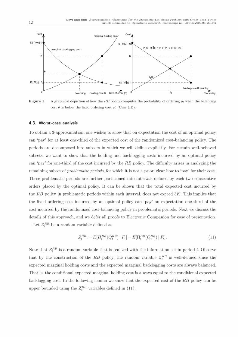
Case (II)
If the balancing cost is less than K, i.e., θt <K, the RB policy orders in period t the holding-cost-K
quantity (i.e., qRBt = qt) with probability pt and nothing with probability 1− pt. That is,
qRBt =
{
qt, with probability pt0, with probability 1− pt
. (6)
The probability pt is computed by solving the following equation
ptK = pt ·E[ΠRBt (qt) | ft] + (1− pt) ·E[ΠRB
t (0) | ft]. (7)
The underlying reason behind the choice of this particular randomization in (7) is that the policy
perfectly balances the three types of costs, namely, marginal holding cost, marginal backlogging
cost and fixed ordering cost associated with the period t. In particular, since we order the holding-
cost-K quantity with probability pt and nothing with probability 1− pt, the conditional expected
marginal holding cost in this case is
E[HRBt (qRB
t ) | ft] = ptE[HRBt (qt) | ft] + (1− pt)E[HRB
t (0) | ft] = ptK. (8)
By the construction of pt in Equation (7), the conditional expected backlogging cost is
E[ΠRBt (qRB
t ) | ft] = ptE[ΠRBt (qt) | ft] + (1− pt)E[ΠRB
t (0) | ft] = ptK. (9)
Since pt is the ordering probability in Case (II), the expected fixed ordering cost is ptK. It can be
shown that Equation (7) has the following solution,
0≤ pt =E[ΠRB
t (0) | ft]
K −E[ΠRBt (qt) | ft] +E[ΠRB
t (0) | ft]< 1. (10)
The inequalities in Equation (10) follows from the fact that θt <K and qt > qt, which implies that
E[ΠRBt (qt) | ft] < E[ΠRB
t (qt) | ft] = θt < K. Figure 1 illustrates how the RB policy computes the
ordering probability pt in Case (II) where θt <K.
This concludes the description of the RB policy. In the next section, we shall show that the RB
policy has an expected worst-case performance guarantee of 3.
Levi and Shi: Approximation Algorithms for the Stochastic Lot-sizing Problem with Order Lead Times12 Article submitted to Operations Research; manuscript no. OPRE-2009-06-260.R2
Figure 1 A graphical depiction of how the RB policy computes the probability of ordering pt when the balancing
cost θ is below the fixed ordering cost K (Case (II)).
4.3. Worst-case analysis
To obtain a 3-approximation, one wishes to show that on expectation the cost of an optimal policy
can ‘pay’ for at least one-third of the expected cost of the randomized cost-balancing policy. The
periods are decomposed into subsets in which we will define explicitly. For certain well-behaved
subsets, we want to show that the holding and backlogging costs incurred by an optimal policy
can ‘pay’ for one-third of the cost incurred by the RB policy. The difficulty arises in analyzing the
remaining subset of problematic periods, for which it is not a-priori clear how to ‘pay’ for their cost.
These problematic periods are further partitioned into intervals defined by each two consecutive
orders placed by the optimal policy. It can be shown that the total expected cost incurred by
the RB policy in problematic periods within each interval, does not exceed 3K. This implies that
the fixed ordering cost incurred by an optimal policy can ‘pay’ on expectation one-third of the
cost incurred by the randomized cost-balancing policy in problematic periods. Next we discuss the
details of this approach, and we defer all proofs to Electronic Companion for ease of presentation.
Let ZRBt be a random variable defined as
ZRBt :=E[HRB
t (QRBt ) | Ft] =E[ΠRB
t (QRBt ) | Ft]. (11)
Note that ZRBt is a random variable that is realized with the information set in period t. Observe
that by the construction of the RB policy, the random variable ZRBt is well-defined since the
expected marginal holding costs and the expected marginal backlogging costs are always balanced.
That is, the conditional expected marginal holding cost is always equal to the conditional expected
backlogging cost. In the following lemma we show that the expected cost of the RB policy can be
upper bounded using the ZRBt variables defined in (11).
Levi and Shi: Approximation Algorithms for the Stochastic Lot-sizing Problem with Order Lead TimesArticle submitted to Operations Research; manuscript no. OPRE-2009-06-260.R2 13
Lemma 1. Let C (RB) be the total cost incurred by the RB policy. Then we have,
E[C (RB)]≤ 3 ·T−L∑
t=1
E[ZRBt ]. (12)
To complete the worst-case analysis, we would like to show that the expected cost of an optimal
policy denoted by OPT is at least∑T−L
t=1 E[ZRBt ]. This will be done by amortizing the cost of OPT
against the cost of the RB policy. In particular, we shall show that on expectation OPT pays for
a large fraction of the cost of the RB policy. In the subsequent analysis, we will use a random
partition of periods t= {1,2, . . . T −L} to the following sets:
The set T1H , {t : Θt ≥K and Y OPTt >Y RB
t } consists of periods in which the balancing cost Θt
exceeds K and the optimal policy had higher inventory position than that of the RB policy after
ordering (recall that if Θt ≥K then the RB policy orders the balancing quantity with probability
1 and the value Y RBt is known deterministically (i.e., realized) with Ft).
The set T1Π , {t : Θt ≥K and Y OPTt ≤ Y RB
t } consists of periods in which the balancing cost
exceeds K and the inventory position of the optimal policy does not exceed that of the RB policy
after ordering (see the comment above regarding T1H).
The set T2H ,
{
t : Θt <K and Y OPTt ≥XRB
t + QRBt
}
consists of periods in which the balancing
cost is less than K and, in such periods, the inventory position of the RB policy after ordering
would be either XRBt if no order was placed, or XRB
t + QRBt if the holding-cost-K quantity is
ordered, depending on the randomized decision of the RB policy. However, the inventory position
of OPT after ordering exceeds even XRBt + QRB
t . (Note again that the quantity QRBt is known
deterministically (i.e., realized) with Ft.)
Analogous to T2H , the set T2Π , {t : Θt <K and XRBt ≥ Y OPT
t } consists of periods in which the
inventory position of OPT after ordering is below XRBt .
The set T2M ,
{
t : Θt <K and XRBt <Y OPT
t <XRBt + QRB
t
}
consists of periods in which the bal-
ancing cost is less than K and the inventory position of OPT after ordering is within (XRBt ,XRB
t +
QRBt ). Thus, whether the RB policy or OPT has more inventory depends on whether the RB
policy placed an order.
Note that the sets (T1H − T2M) are disjoint and the union makes a complete set. Conditioning
on ft, it is already known which part of the partition period t belongs.
Next we will show that the total holding cost incurred by OPT is higher than the marginal
holding cost incurred by the RB policy in periods that belong to T1H
⋃
T2H , and that the total
backlogging cost incurred by OPT is higher than the backlogging cost incurred by the RB policy
associated with periods within T1Π
⋃
T2Π.
Levi and Shi: Approximation Algorithms for the Stochastic Lot-sizing Problem with Order Lead Times14 Article submitted to Operations Research; manuscript no. OPRE-2009-06-260.R2
Lemma 2. The overall holding cost and backlogging cost incurred by OPT are denoted by HOPT
and ΠOPT , respectively. Then we have, with probability 1,
HOPT ≥∑
t
HRBt ·1(t∈T1H
⋃
T2H), ΠOPT ≥∑
t
ΠRBt ·1(t∈T1Π
⋃
T2Π). (13)
Note that the periods in the set T2M introduce some uncertainties in the relation between the
inventory positions after ordering of the RB policy and OPT . Thus, we are unable to carry out an
analysis similar to Lemma 2. For this reason, we call T2M a problematic set of periods. Naturally,
we also define the non-problematic set of periods to be TN =T1H
⋃
T1Π
⋃
T2Π
⋃
T2H . The analysis
of the problematic periods in the set T2M will be done in two steps. In the first step, we will
conceptually create a bank account A that will be used to pay some of the cost of the RB policy in
these problematic periods. In particular, for each period t∈T2M , we borrow an amount of ZRBt from
the bank account. Thus, the total amount of borrowing from the bank is given by A=∑
t∈T2MZRB
t ,
and so E[A] =E [∑
tZRB
t ·1(t∈T2M)].
The following lemma shows that, with the borrowed amount A from the bank, the overall holding
cost and backlogging cost incurred by OPT exceed∑T−L
t=1 E[ZRBt ]. The next step will be to show
that E[A] is at most the expected fixed ordering cost incurred by OPT . That is,
E[A]≤E
[
T−L∑
t=1
K ·1(QOPTt > 0)
]
. (14)
Lemma 3. The expected holding cost and backlogging cost incurred by OPT plus the expected
amount borrowed from the bank account A are at least∑T−L
t=1 E[ZRBt ]. That is, the following inequal-
ity holds
E[(
HOPT +ΠOPT)
+A]
≥T−L∑
t=1
E[ZRBt ]. (15)
By Lemmas 1 and 3, the overall holding and backlogging costs incurred by OPT , plus the
borrowed amount A from the bank, account on expectation for one-third of the overall expected
costs incurred by the RB policy. To complete the worst-case analysis, we will show in Lemma 4 that
the expected amount borrowed from the bank account does not exceed the expected fixed ordering
cost incurred by OPT , i.e., E[
∑T−L
t=1 K ·1(QOPTt > 0)
]
. We will highlight the key steps involved in
proving this lemma. We decompose the problematic periods in the set T2M into intervals between
ordering points of OPT , and we want to show that, for each such interval, the fixed ordering cost K
incurred by OPT will cover the expected amount borrowed from the bank in periods that belong
to set T2M . Conditioning on f−
T (the entire evoluation of the system excluding the randomized
decisions of the RB policy), we construct a decision tree based on the randomized decisions of the
RB policy. We then show that, by a tree traversal argument and Lemma 5, the expected borrowing
from the problematic nodes (which belong to the set T2M) within an interval between ordering
points of OPT does not exceed K.
Levi and Shi: Approximation Algorithms for the Stochastic Lot-sizing Problem with Order Lead TimesArticle submitted to Operations Research; manuscript no. OPRE-2009-06-260.R2 15
Lemma 4. The following inequality holds
E [A]≤E
[
T−L∑
t=1
K ·1(QOPTt > 0)
]
. (16)
In other words, the expected borrowing E[A] is less than the total expected fixed ordering cost
incurred by OPT .
Lemma 5. Let {pl}∞
l=1 satisfy the condition 0≤ pl ≤ 1 for all l. Then the following inequality holds,
p21 +∞∑
l=2
{(
l−1∏
s=1
(1− ps)
)
pl
(
l∑
k=1
pk
)}
≤ 1. (17)
As an immediate consequence of Lemmas 3 and 4, we obtain the following lemma and theorem.
Lemma 6. Let C (OPT ) be the total cost incurred by the cost-balancing policy RB. Then we have,
E[C (OPT )]≥T−L∑
t=1
E[ZRBt ]. (18)
Theorem 1. For each instance of the stochastic lot-sizing problem, the expected cost of the ran-
domized cost-balancing policy RB is at most three times the expected cost of an optimal policy
OPT , i.e.,
E[C (RB)]≤ 3 ·E[C (OPT )]. (19)
5. Numerical Experiments
The randomized cost-balancing policies described above can be parameterized to obtain general
classes of policies, respectively. The worst-case analysis discussed above can then be viewed as
choosing parameter values that perform well against any possible instance. In contrast, find the
‘best’ parameter values, for each given instance. This gives rise to policies that have at least the same
worst-case performance guarantees, but are likely to work better empirically, since we can refine the
parameters according to the specific instance being solved. Using simulation based optimization,
we have implemented this approach and tested the empirical performance of the resulting policies.
The policies were tested under the model of advanced demand information proposed by Gallego
and Ozer (2001) and Ozer and Wei (2004). To the best of our knowledge, these are the few papers
that report computational results (by brute-force backward induction algorithm) on the stochastic
lot-sizing problem with correlated demands.
5.1. Parameterized policies.
We describe a class of parameterized policies involving parameters β, γ and η where β controls
the holding-cost-βK quantity, γ controls the ratio of marginal holding costs and backlogging costs
and η controls the level of expected backlogging cost resulting from not ordering.
Levi and Shi: Approximation Algorithms for the Stochastic Lot-sizing Problem with Order Lead Times16 Article submitted to Operations Research; manuscript no. OPRE-2009-06-260.R2
• The balancing quantity qt that solves E[HRBt (qt) | ft] = γ ·E[ΠRB
t (qt) | ft] := θt.
• The holding-cost-βK quantity qt that solves E[HRBt (qt) | ft] = β ·K.
• Compute E[ΠRBt (qt) | ft], and η ·E[ΠRB
t (0) | ft].
(I) If θt ≥ β ·K, the RB policy orders qRBt = qt with probability pt = 1 in period t.
(II) If θt <β ·K, the RB policy orders qRBt = qt with probability pt and order nothing with proba-
bility 1−pt in period t, where the probability pt =η ·E[ΠRB
t (0) | ft]
β ·K −E[ΠRBt (qt) | ft] + η ·E[ΠRB
t (0) | ft].
Since T is relatively small, we also introduce an end-of-horizon rule. Suppose we are in period t,
we estimate the total expected cumulative backlogging cost (assuming no orders are placed) over
the interval [t, T ]. If this amount is less than K, we do not order in period t.
5.2. Experiment Design
Under advance information model, the demand vector in each period t is observed as Dt =
(Dt,t, . . . ,Dt,t+N) where Dt,s represents order placed by customers during period t for future peri-
ods s ∈ {t, . . . , t+N} and N is the length of the information horizon over which we have advance
demand information. Note that Dt is a random vector and is realized only at the end of period t.
At the beginning of period t, the demand to prevail in a future period s (s≥ t) can be divided into
two parts: the observed demand vector∑t−1
r=s−NDr,s and the unobserved demand vector
∑s
r=tDr,s.
As a result, this introduces a correlation between period demands (however the conditional joint
distribution of the future demands is known in each period t). The state space of the proposed
dynamic programming formulation contains the inventory position and the observed demand vec-
tor which explodes exponentially with the length of the information horizon N when N >L+ 2.
Gallego and Ozer (2001) verified some structural properties of the dynamic program via numerical
studies for a number of small instances. The experiments that we performed expand their numeri-
cal studies by incorporating non-zero lead times as well as longer planning horizons. Following the
methodology of Aviv and Federgruen (2001), we generated a total of 90 instances to test the qual-
ity of the randomized-balancing heuristics compared to the optimal cost. The instances we used
have the following combination of parameters: T = 12,15, L= 0,1,2, N = L+2, K = 0,5,50,100,
h = 1,2,3,6, p = 1,3,6,9 and (Dt,t,Dt,t+1,Dt,t+2) are modeled by Poisson random variables with
mean λ0, λ1, λ2.
5.3. Algorithmic complexity
We describe the procedures of finding the optimal parameters for a specific instance of the problem.
First, assume that there exists a positive constant U such that the optimal parameters β∗, γ∗, η∗
are upper bounded by U . In addition, we discretize U with some step-size ∆, i.e., β,γ, η ∈ [0,U ]
can only take values as integer multiples of ∆. Then we conduct an exhaustive search on a cube of
Levi and Shi: Approximation Algorithms for the Stochastic Lot-sizing Problem with Order Lead TimesArticle submitted to Operations Research; manuscript no. OPRE-2009-06-260.R2 17
U ×U ×U for the parameters β, γ and η. In our numerical studies, U = 10 and ∆= 0.1 are chosen
to be the upper bound and the resolution for discretization, respectively. The algorithm runs on
every point on this cube, simulates the cost of each parameterized policy and returns the best
possible (β∗, γ∗, η∗) that minimize the cost. Secondly, assume that there exists a positive constant
U that serves an upper bound on the balancing and hold-cost-K quantities. For each t= 1, . . . , T ,
the complexity for evaluating marginal holding cost is O(T ) and the complexity for carrying out
bisection search is O(log U). The algorithm runs in O(T 2 log U), for each set of parameters (β, γ,
η). Hence, the algorithm that returns both the optimal parameters and the lowest cost runs in
O(U 3∆−3T 2 log U) ≈ O(T 2) since U 3∆−3 log U is some positive constant. For all tested instances
with T = 12, the average CPU time per test instance on a Pentium 1.58GHz PC is 233s. In contrast,
the dynamic programming algorithm takes 1840s on average per test instance.
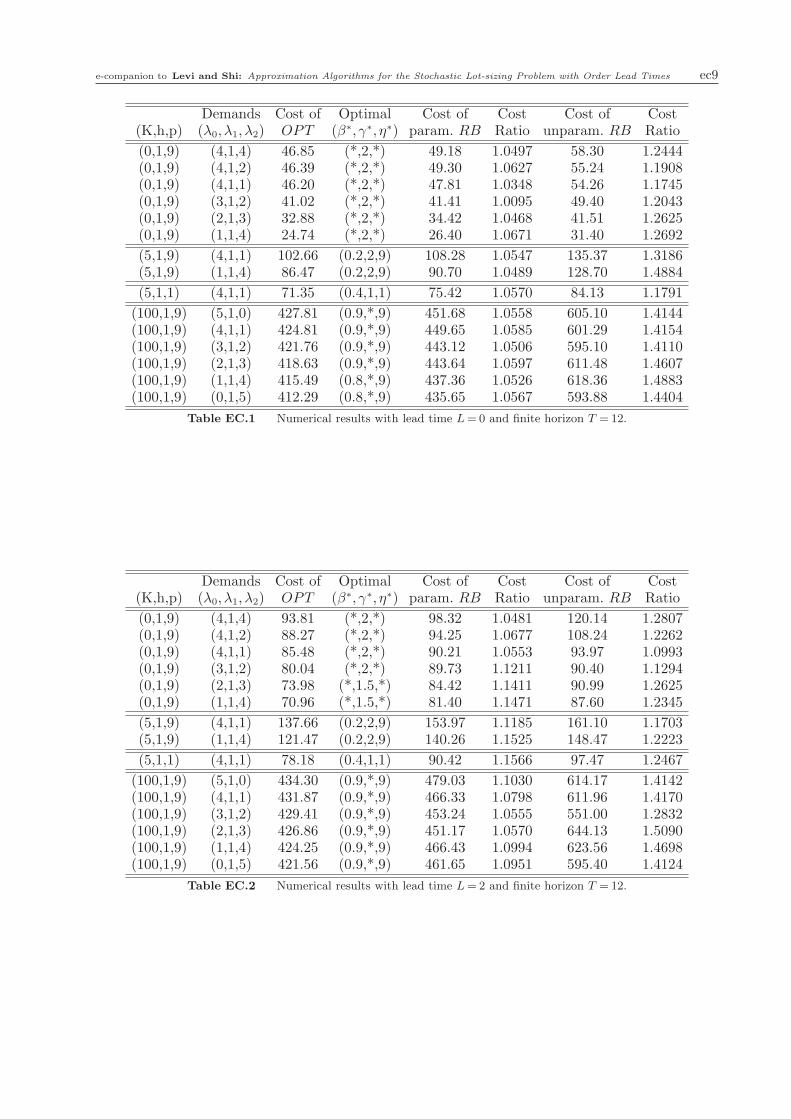
5.4. Numerical results
The numerical results with (T,L) = (12,0), (T,L) = (12,2) and (T,L) = (15,0) are tabulated in
Table EC.1, Table EC.2 and Table EC.3, respectively (refer to Electronic Companion). The (∗) in
both tables indicates that the designated parameters can take arbitrary numbers without affecting
the optimal values of the parameterized policy. It is observed that (β∗, η∗) = (∗,∗) in all instances
where K = 0, since the holding-cost-β∗K quantity is trivially 0 and therefore the algorithm only
considers the balancing quantities. In some instances where K is relatively large and the holding-
cost-β∗K quantity is near-optimal, it is observed that γ∗ = (∗) implying that the algorithm only
orders the holding-cost-β∗K quantities. For the rest of instances, the algorithm uses both the
balancing quantity and the holding-cost-K quantity.
In the case where L = 0, on average the parameterized RB policy performs within 4.6% and
always within 7% of the optimal cost for T = 12,15. The numerical results show that the per-
formance of the parameterized RB policy is insensitive to the planning horizon T . Moreover, the
optimal parameters in the parameterized RB policy are intuitive: β controls the quantity of each
order; γ controls the ratio in which the marginal holding cost is balanced against the marginal
backlogging cost; η controls the weight put on the do-nothing backlogging cost resulted from not
ordering. The optimal η∗ = 9 coincides with the ratio of p to h, which implies that more weight
should be put on backlogging cost so that the ordering probability can be increased. The optimal
γ∗ = 2 suggests that the marginal holding cost should be twice the backlogging cost. The optimal β∗
is close to 1 when K is large, implying that using the holding-cost-K quantity is near optimal. The
unparameterized RB policy (i.e., (β,γ, η) = (1,1,1)) performs on average within 27% and always
within 50% error of optimal cost, which is significantly better than the theoretical worst-case per-
formance guarantee of 3. The cost ratio is observed to be decreasing in the magnitude of fixed
Levi and Shi: Approximation Algorithms for the Stochastic Lot-sizing Problem with Order Lead Times18 Article submitted to Operations Research; manuscript no. OPRE-2009-06-260.R2
ordering cost K. In the case where L= 2, the parameterized RB policy performs on average within
10% and always within 16% error of the optimal cost. The optimal parameters are similar to those
in L= 0. The deviation from the optimal cost is resulted from stocking more inventory units by
the RB policy, as the lead time induces more uncertainty in future demands. The unparameterized
RB policy performs within 50% (on average 29%) error of optimal cost. It is also noted that the
average CPU time of running the RB policy is insensitive to the planning horizon T .
Acknowledgments
The authors thank the Associate Editor and the anonymous referees for a handful of constructive comments
that improved the content and exposition of this paper. The research of the authors was partially supported
by NSF grants DMS-0732175 and CMMI-0846554 (CAREER Award), an AFOSR award FA9550-08-1-0369,
an SMA grant and the Buschbaum Research Fund of MIT.
References
Aviv, Y., A. Federgruen. 2001. Capacitated multi-item inventory systems with random and seasonally
fluctuating demands: Implications for postponement strategies. Management Science 47(4) 512–531.
Bollapragada, S., T. E. Morton. 1999. A simple heuristic for computing nonstationary (s,S) policies. Oper-
ations Research 47(4) 576–584.
Borodin, A., R. El-Yaniv. 1998. Online Computation and Competitive Analysis . Cambridge University Press.
Bouchard, B., N. E. Karoui, N. Touzi. 2005. Maturity randomized for stochastic control problems. The
Annals of Applied Probability 15(4) 2575–2605.
Cheng, F., S. Sethi. 1997. Optimality of (s, S) policies in inventory models with markovian demand. Oper-
ations Research 45(6) 931–939.
Federgruen, A., Y. S. Zheng. 1991. An efficient algorithm for computing an optimal (r, Q) policy in continuous
review stochastic inventory systems. Operations Research 40(4) 808–813.
Federgruen, A., P. H. Zipkin. 1984. An efficient algorithm for computing optimal (s, S) policies. Operations
Research 32(6) 1268–1285.
Gallego, G., O. Ozer. 2001. Integrating replenishment decisions with advance demand information. Man-
agement Science 47(10) 1344–1360.
Gavirneni, S. 2001. An efficient heuristic for inventory control when the customer is using a (s, S) policy.
Operations Research Letters 28(4) 187–192.
Guan, Y., A. J. Miller. 2008a. Polynomial time algorithms for stochastic uncapacitated lot-sizing problems.
Operations Research 56(5) 1172–1183.
Guan, Y., A. J. Miller. 2008b. A polynomial time algorithms for the stochastic uncapacitated lot-sizing
problem with backlogging. IPCO 2008, volume 5035 of Lecture Notes in Computer Science 450–462.
Levi and Shi: Approximation Algorithms for the Stochastic Lot-sizing Problem with Order Lead TimesArticle submitted to Operations Research; manuscript no. OPRE-2009-06-260.R2 19
Levi, R., G. Janakiraman, M. Nagarajan. 2008a. A 2-approximation algorithm for stochastic inventory
control models with lost-sales. Mathematics of Operations Research 33(2) 351–374.
Levi, R., M. Pal, R. O. Roundy, D. B. Shmoys. 2007. Approximation algorithms for stochastic inventory
control models. Mathematics of Operations Research 32(2) 284–302.
Levi, R., R. O. Roundy, D. B. Shmoys, M. Sviridenko. 2008b. A constant approximation algorithm for the
one-warehouse multi-retailer problem. Management Sceince 54(4) 763–776.
Levi, R., R. O. Roundy, D. B. Shmoys, V. A. Truong. 2008c. Approximation algorithms for capacitated
stochastic inventory models. Operations Research 56(5) 1184–1199.
Levi, R., R. O. Roundy, V. A. Truong. 2005. Provably near-optimal balancing policies for multi-echelon
stochastic inventory control models. Working Paper.
Motwani, R., P. Raghavan. 1995. Randomized algorithms. Cambridge University Press .
Ozer, O., W. Wei. 2004. Inventory control with limited capacity and advance demand information. Operations
Research 52(6) 988–1000.
Prandini, M., J. Lygeros, A. Nilim, S. Sastry. 1999. Randomized algorithms for probabilistic aircraft conflict
detection. IEEE Conference on Decision and Control 3 2444–2449.
Rust, J. 1997. Using randomization to break the curse of dimensionality. Econometrica 65(3) 487–516.
Scarf, H. 1960. The optimality of (S,s) policies in the dynamic inventory problem. Mathematical Methods in
Social Sciences .
Shmoys, D., C. Swamy. 2006. An approximation scheme for stochastic linear programming and its application
to stochastic integer programs. Journal of the ACM 53(6) 978–1012.
Shmoys, D., K. Talwar. 2008. A constant approximation algorithm for the a priori traveling salesman
problem. Integer Programming and Combinatorial Optimization 5035 331–343. Lecture Notes in
Computer Science.
Song, J., P. H. Zipkin. 1993. Inventory control in a fluctuating demand environment. Operations Research
41(2) 351–370.
Teo, C. P., D. Bertsimas. 1996. Improved randomized approximation algorithms for lot-sizing problems.
Proceedings of the 5th International IPCO Conference on Integer Programming and Combinatorial
Optimization 359–373.
Veinott, A. 1966. On the optimality of (s,S) inventory policies: new conditions and a new proof. SIAM J.
Appl. Math 14(5) 1067–1083.
e-companion to Levi and Shi: Approximation Algorithms for the Stochastic Lot-sizing Problem with Order Lead Times ec1
This page is intentionally blank. Proper e-companion title
page, with INFORMS branding and exact metadata of the
main paper, will be produced by the INFORMS office when
the issue is being assembled.
ec2 e-companion to Levi and Shi: Approximation Algorithms for the Stochastic Lot-sizing Problem with Order Lead Times
Electronic Companion
EC.1. Proofs of Technical Lemmas and Theorems
LEMMA 1. Let C (RB) be the total cost incurred by the RB policy. Then we have,
E[C (RB)]≤ 3 ·T−L∑
t=1
E[ZRBt ]. (EC.1)
Proof of Lemma 1. Using the marginal cost accounting in Equation (4) and standard arguments
of conditional expectations, we express
E[C (RB)] =T−L∑
t=1
E[HRBt (QRB
t )+ΠRBt (QRB
t )+K ·1(QRBt > 0)] (EC.2)
=T−L∑
t=1
E[
E[HRBt (QRB
t )+ΠRBt (QRB
t )+K ·1(QRBt > 0) | Ft]
]
=T−L∑
t=1
E[2ZRBt +PtK]≤ 3
T−L∑
t=1
E[ZRBt ].
The third equality follows directly from (11). To establish the first inequality in (EC.2) above, we
shall show that Zt ≥ PtK almost surely. That is, for each ft ∈ Ft, zt ≥ ptK. Given any information
set ft, all the quantities xt, θt, ψt, φt and pt defined above are known deterministically. We split
the analysis into two cases:
1. If θt ≥K, then qRBt = qt (the balancing quantity) with probability pt = 1 implying zt = θt ≥K.
The claim follows.
2. If θt <K, then qRBt = qt (the holding-cost-K quantity) with probability pt and q
RBt = 0 with
1− pt. Thus, by Equations (8) and (9), we have zt = ptK, and the claim follows.
This concludes the proof of the lemma. �
LEMMA 2. The overall holding cost and backlogging cost incurred by OPT are denoted by HOPT
and ΠOPT , respectively. Then we have, with probability 1,
HOPT ≥∑
t
HRBt ·1(t∈T1H
⋃
T2H), ΠOPT ≥∑
t
ΠRBt ·1(t∈T1Π
⋃
T2Π). (EC.3)
Proof of Lemma 2. The proof is identical to Lemmas 4.2 and 4.3 in Levi et al. (2007). �
LEMMA 3. The expected holding cost and backlogging cost incurred by OPT plus the expected amount
borrowed from the bank account A are at least∑T−L
t=1 E[ZRBt ]. That is, The following inequality
holds
E[(
HOPT +ΠOPT)
+A]
≥T−L∑
t=1
E[ZRBt ]. (EC.4)
e-companion to Levi and Shi: Approximation Algorithms for the Stochastic Lot-sizing Problem with Order Lead Times ec3
Proof of Lemma 3. Using linearity of expectation, it suffices to show
E[
HOPT +ΠOPT]
≥T−L∑
t=1
E[
1(t∈TN) ·ZRBt
]
. (EC.5)
Using Lemma 2 and standard arguments of condition expectations, we have
E[HOPT ] ≥ E
[
∑
t
HRBt ·1(t∈T1H
⋃
T2H)
]
(EC.6)
= E
[
E
[
∑
t
HRBt ·1(t∈T1H
⋃
T2H) | Ft
]]
= E
[
∑
t
ZRBt ·1(t∈T1H
⋃
T2H)
]
.
Similarly, we also have
E[ΠOPT ] ≥ E
[
∑
t
ZRBt ·1(t∈T1Π
⋃
T2Π)
]
. (EC.7)
Equation (EC.5) follows from summing up Equations (EC.6) and (EC.7). �
LEMMA 4. The following inequality holds
E [A]≤E
[
T−L∑
t=1
K ·1(QOPTt > 0)
]
. (EC.8)
In other words, the expected borrowing E[A] is less than the total expected fixed ordering cost
incurred by OPT .
Proof of Lemma 4. First we define the reduced information set f−
t to be the information up to
period t excluding the randomized decisions of the RB policy over [1, t−1]. In particular, given the
entire evolution of demand f−
T , the sequence of orders placed by OPT is known deterministically.
Let 1≤ t1 < t2 < . . . < tn ≤ T −L be the periods in which OPT placed n= n | f−
T orders sequentially.
Let t0 = 0 and tn+1 = T −L+1. We shall show that there are no problematic periods within (t0, t1)
and that, for each i= 1, . . . n, the expected borrowing within the interval [ti, ti+1) does not exceed
K. That is,
(t0, t1)⋂
T2M = ∅, (EC.9)
E
∑
t∈[ti,ti+1)⋂
T2M
ZRBt | f−
T
≤ K. (EC.10)
It is important to note that f−
T does not include the randomized decisions of the RB policy.
Thus, the set T2M is still random and so is the amount borrowed from the bank. In particular,
ec4 e-companion to Levi and Shi: Approximation Algorithms for the Stochastic Lot-sizing Problem with Order Lead Times
the expectation in Equation (EC.10) is taken with respect to the randomized decisions of the RB
policy. Equations (EC.10) and (EC.9) imply that, for each f−
T ,
E
∑
t∈T2M
ZRBt | f−
T
≤K ·n | f−
T =K ·n, (EC.11)
and therefore
E[A]≤K ·E[N ] =E
[
T−L∑
t=1
K ·1(QOPTt > 0)
]
. (EC.12)
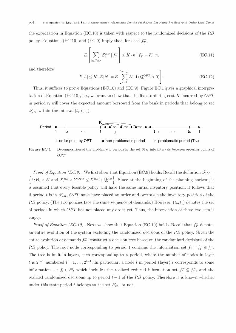
Thus, it suffices to prove Equations (EC.10) and (EC.9). Figure EC.1 gives a graphical interpre-
tation of Equation (EC.10), i.e., we want to show that the fixed ordering cost K incurred by OPT
in period ti will cover the expected amount borrowed from the bank in periods that belong to set
T2M within the interval [ti, ti+1).
Figure EC.1 Decomposition of the problematic periods in the set T2M into intervals between ordering points of
OPT
Proof of Equation (EC.9). We first show that Equation (EC.9) holds. Recall the definition T2M ={
t : Θt <K and XRBt <Y OPT
t ≤XRBt + QRB
t
}
. Since at the beginning of the planning horizon, it
is assumed that every feasible policy will have the same initial inventory position, it follows that
if period t is in T2M , OPT must have placed an order and overtaken the inventory position of the
RB policy. (The two policies face the same sequence of demands.) However, (t0, t1) denotes the set
of periods in which OPT has not placed any order yet. Thus, the intersection of these two sets is
empty.
Proof of Equation (EC.10). Next we show that Equation (EC.10) holds. Recall that f−
T denotes
an entire evolution of the system excluding the randomized decisions of the RB policy. Given the
entire evolution of demands f−
T , construct a decision tree based on the randomized decisions of the
RB policy. The root node corresponding to period 1 contains the information set f1 = f−
1 ∈ f−
T .
The tree is built in layers, each corresponding to a period, where the number of nodes in layer
t is 2t−1 numbered l = 1, . . . ,2t−1. In particular, a node l in period (layer) t corresponds to some
information set ft ∈ Ft which includes the realized reduced information set f−
t ⊆ f−
T , and the
realized randomized decisions up to period t− 1 of the RB policy. Therefore it is known whether
under this state period t belongs to the set T2M or not.
e-companion to Levi and Shi: Approximation Algorithms for the Stochastic Lot-sizing Problem with Order Lead Times ec5
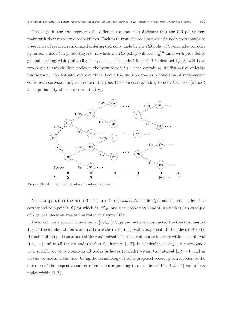
The edges in the tree represent the different (randomized) decisions that the RB policy may
make with their respective probabilities. Each path from the root to a specific node corresponds to
a sequence of realized randomized ordering decisions made by the RB policy. For example, consider
again some node l in period (layer) t in which the RB policy will order qRBtl units with probability
ptl and nothing with probability 1 − ptl; then the node l in period t (denoted by tl) will have
two edges to two children nodes in the next period t+ 1 each containing its distinctive ordering
information. Conceptually one can think about the decision tree as a collection of independent
coins, each corresponding to a node in the tree. The coin corresponding to node l at layer (period)
t has probability of success (ordering) ptl.
Figure EC.2 An example of a general decision tree
Next we partition the nodes in the tree into problematic nodes (pn nodes), i.e., nodes that
correspond to a pair (t, ft) for which t∈T2M , and non-problematic nodes (nn nodes). An example
of a general decision tree is illustrated in Figure EC.2.
Focus now on a specific time interval [ti, ti+1). Suppose we have constructed the tree from period
1 to T ; the number of nodes and paths are clearly finite (possibly exponential). Let the set G to be
the set of all possible outcomes of the randomized decisions in all nodes in layers within the interval
[1, ti − 1] and in all the nn nodes within the interval [1, T ]. In particular, each g ∈ G corresponds
to a specific set of outcomes in all nodes in layers (periods) within the interval [1, ti − 1] and in
all the nn nodes in the tree. Using the terminology of coins proposed before, g corresponds to the
outcome of the respective subset of coins corresponding to all nodes within [1, ti − 1] and all nn
nodes within [1, T ].
ec6 e-companion to Levi and Shi: Approximation Algorithms for the Stochastic Lot-sizing Problem with Order Lead Times
Conditioning on some g ∈ G induces a path from the root of the tree (in period 1) up to the
earliest pn node, say j, where j corresponds to the period (layer) of that node. Here we abuse the
notation ignoring the index of the node within layer j. (Namely, the exact value will be je for some
e.) It is straightforward to see that j ≥ ti. If j falls outside the interval [ti, ti+1), i.e., j ≥ ti+1, it
follows that there are no pn nodes within the interval [ti, ti+1), and there is no borrowing over the
interval. Assume now that j falls within the interval [ti, ti+1) (j can possibly be in period (layer)
ti). We will show that the expected borrowing does not exceed K. That is,
E
∑
s∈[j,ti+1)⋃
T2M
ZRBs | f−
T , g
≤K. (EC.13)
The proof of Equation (EC.10) will then follow.
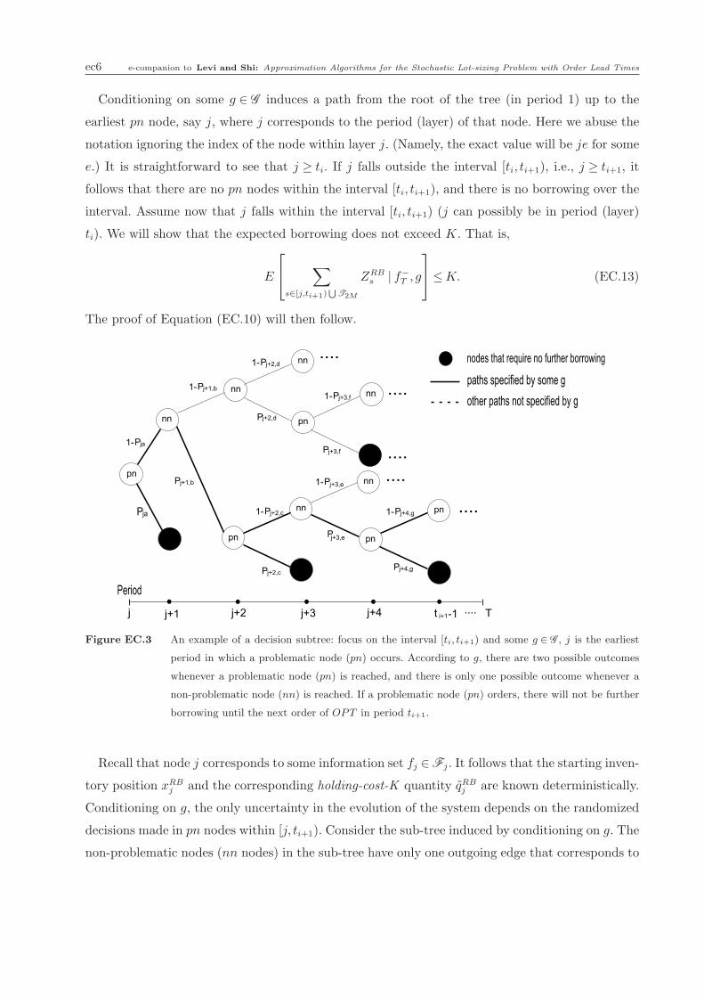
Figure EC.3 An example of a decision subtree: focus on the interval [ti, ti+1) and some g ∈ G , j is the earliest
period in which a problematic node (pn) occurs. According to g, there are two possible outcomes
whenever a problematic node (pn) is reached, and there is only one possible outcome whenever a
non-problematic node (nn) is reached. If a problematic node (pn) orders, there will not be further
borrowing until the next order of OPT in period ti+1.
Recall that node j corresponds to some information set fj ∈Fj . It follows that the starting inven-
tory position xRBj and the corresponding holding-cost-K quantity qRB
j are known deterministically.
Conditioning on g, the only uncertainty in the evolution of the system depends on the randomized
decisions made in pn nodes within [j, ti+1). Consider the sub-tree induced by conditioning on g. The
non-problematic nodes (nn nodes) in the sub-tree have only one outgoing edge that corresponds to
e-companion to Levi and Shi: Approximation Algorithms for the Stochastic Lot-sizing Problem with Order Lead Times ec7
the decision (order/no-order) specified by g to that node. The problematic nodes (pn nodes) have
two outgoing edges corresponding to the order/no-order decisions, respectively. (Recall that g does
not specify the decisions in these nodes.) Moreover, each pn node s∈ [j, ti+1) is associated with the
probability ps of ordering. (We again abuse the notation introduced before and omit the index e
of the node within the layer/period.) An example of a decision subtree specified by some g ∈ G is
illustrated in Figure EC.3. Any sequence of randomized outcomes corresponding to the decisions
in the pn nodes induces a path of evolution of the system. The resulting cumulative borrowing
from the bank account A, corresponding to this path, is equal to K times the sum of probabilities
associated with the pn nodes in this path. (For each pn node s in the path, the borrowing is equal
to psK = zs.)
Next we claim that the sub-tree defined above includes at most one pn node in each layer (period).
This follows from the fact that any path between two pn nodes r, s such that j ≤ r < s < ti+1 in
the tree includes only no-ordering edges of pn nodes. To see why the latter is true, observe that
if an order is placed by the RB policy in a pn node, the resulting inventory position of the RB
policy is higher than OPT . Since both policies face the same sequence of demands, the RB policy
will not have higher inventory position than OPT at least until the next order placed by OPT .
This excludes the existence of pn nodes in subsequent periods until OPT places another order, i.e.,
beyond period ti+1 − 1.
In light of the latter observation, we re-number all the pn nodes in the sub-tree as 1,2, . . . ,M
(where 1 corresponds to j, specified before). Moreover, it follows that the probability to arrive at
node m = 1, . . . ,M and borrow pmK is equal to∏m−1
s=1 (1− ps). (This probability corresponds to
no-ordering decisions in all the pn nodes prior to m.) The total expected borrowing is then
K ·
{
p21 +M∑
m=2
{(
m−1∏
s=1
(1− ps)
)
pm
(
m∑
k=1
pk
)}}
. (EC.14)
Observe that the probability to borrow exactly K ·∑m
k=1 pk is equal to(
∏m−1
s=1 (1− ps))
pm. More-
over, we have already shown that the expression in (EC.14) is bounded above by K (see Lemma
5). This concludes the proof of the lemma. �
LEMMA 5. Let {pl}∞
l=1 satisfy the condition 0≤ pl ≤ 1 for all l. Then the following inequality holds,
p21 +∞∑
l=2
{(
l−1∏
s=1
(1− ps)
)
pl
(
l∑
k=1
pk
)}
≤ 1. (EC.15)
Proof of Lemma 5. We construct an increasing sequence {am} where
am = p21 +m∑
l=2
{(
l−1∏
s=1
(1− ps)
)
pl
(
l∑
k=1
pk
)}
. (EC.16)
ec8 e-companion to Levi and Shi: Approximation Algorithms for the Stochastic Lot-sizing Problem with Order Lead Times
For each m, if we replace pm by 1, we get
am = p21 +m−1∑
l=2
{(
l−1∏
s=1
(1− ps)
)
pl
(
l∑
k=1
pk
)}
+
(
m−1∏
s=1
(1− ps)
)(
1+m−1∑
k=1
pk
)
, (EC.17)
such that am ≤ am. Next we will show by induction that am ≤ 1 for all m from which the proof of
the lemma follows. It is straightforward to verify a1, a2 ≤ 1. Assume that am ≤ 1 for some m∈Z+,
we will show that am+1 ≤ 1.
am+1 = p21 +m∑
l=2
{(
l−1∏
s=1
(1− ps)
)
pl
(
l∑
k=1
pk
)}
+
(
m∏
s=1
(1− ps)
)(
1+m∑
k=1
pk
)
(EC.18)
= am−1 +
(
m−1∏
s=1
(1− ps)
)
pm
(
m∑
k=1
pk
)
+
(
m∏
s=1
(1− ps)
)(
1+m∑
k=1
pk
)
= am−1 +
(
m−1∏
s=1
(1− ps)
)[(
1+m∑
k=1
pk
)
(1− pm)+ pm
m∑
k=1
pk
]
= am−1 +
(
m−1∏
s=1
(1− ps)
)(
1+m−1∑
k=1
pk
)
= am ≤ 1.
Hence the claim follows by induction. �
EC.2. Performance of the proposed algorithms
The first two columns specify the test instances, namely, fixed ordering cost K, per-unit holding
cost h, per-unit backlogging cost p and demand rate vector λ. The third column shows the cost
incurred by the optimal policy. The fourth column shows the optimal parameters of paramerized
RB policy. The fifth column shows the cost incurred by the parameterized RB policy. The sixth
column shows the cost ratio of the parameterized RB policy to the optimal policy. The seventh
column shows the cost of unparameterized RB policy (i.e., the original policy without parameter
optimization). The eighth columns shows the cost ratio of the unparameterized RB policy to the
optimal policy.
e-companion to Levi and Shi: Approximation Algorithms for the Stochastic Lot-sizing Problem with Order Lead Times ec9
Demands Cost of Optimal Cost of Cost Cost of Cost(K,h,p) (λ0, λ1, λ2) OPT (β∗, γ∗, η∗) param. RB Ratio unparam. RB Ratio
(0,1,9) (4,1,4) 46.85 (*,2,*) 49.18 1.0497 58.30 1.2444(0,1,9) (4,1,2) 46.39 (*,2,*) 49.30 1.0627 55.24 1.1908(0,1,9) (4,1,1) 46.20 (*,2,*) 47.81 1.0348 54.26 1.1745(0,1,9) (3,1,2) 41.02 (*,2,*) 41.41 1.0095 49.40 1.2043(0,1,9) (2,1,3) 32.88 (*,2,*) 34.42 1.0468 41.51 1.2625(0,1,9) (1,1,4) 24.74 (*,2,*) 26.40 1.0671 31.40 1.2692
(5,1,9) (4,1,1) 102.66 (0.2,2,9) 108.28 1.0547 135.37 1.3186(5,1,9) (1,1,4) 86.47 (0.2,2,9) 90.70 1.0489 128.70 1.4884
(5,1,1) (4,1,1) 71.35 (0.4,1,1) 75.42 1.0570 84.13 1.1791
(100,1,9) (5,1,0) 427.81 (0.9,*,9) 451.68 1.0558 605.10 1.4144(100,1,9) (4,1,1) 424.81 (0.9,*,9) 449.65 1.0585 601.29 1.4154(100,1,9) (3,1,2) 421.76 (0.9,*,9) 443.12 1.0506 595.10 1.4110(100,1,9) (2,1,3) 418.63 (0.9,*,9) 443.64 1.0597 611.48 1.4607(100,1,9) (1,1,4) 415.49 (0.8,*,9) 437.36 1.0526 618.36 1.4883(100,1,9) (0,1,5) 412.29 (0.8,*,9) 435.65 1.0567 593.88 1.4404
Table EC.1 Numerical results with lead time L= 0 and finite horizon T = 12.
Demands Cost of Optimal Cost of Cost Cost of Cost(K,h,p) (λ0, λ1, λ2) OPT (β∗, γ∗, η∗) param. RB Ratio unparam. RB Ratio
(0,1,9) (4,1,4) 93.81 (*,2,*) 98.32 1.0481 120.14 1.2807(0,1,9) (4,1,2) 88.27 (*,2,*) 94.25 1.0677 108.24 1.2262(0,1,9) (4,1,1) 85.48 (*,2,*) 90.21 1.0553 93.97 1.0993(0,1,9) (3,1,2) 80.04 (*,2,*) 89.73 1.1211 90.40 1.1294(0,1,9) (2,1,3) 73.98 (*,1.5,*) 84.42 1.1411 90.99 1.2625(0,1,9) (1,1,4) 70.96 (*,1.5,*) 81.40 1.1471 87.60 1.2345
(5,1,9) (4,1,1) 137.66 (0.2,2,9) 153.97 1.1185 161.10 1.1703(5,1,9) (1,1,4) 121.47 (0.2,2,9) 140.26 1.1525 148.47 1.2223
(5,1,1) (4,1,1) 78.18 (0.4,1,1) 90.42 1.1566 97.47 1.2467
(100,1,9) (5,1,0) 434.30 (0.9,*,9) 479.03 1.1030 614.17 1.4142(100,1,9) (4,1,1) 431.87 (0.9,*,9) 466.33 1.0798 611.96 1.4170(100,1,9) (3,1,2) 429.41 (0.9,*,9) 453.24 1.0555 551.00 1.2832(100,1,9) (2,1,3) 426.86 (0.9,*,9) 451.17 1.0570 644.13 1.5090(100,1,9) (1,1,4) 424.25 (0.9,*,9) 466.43 1.0994 623.56 1.4698(100,1,9) (0,1,5) 421.56 (0.9,*,9) 461.65 1.0951 595.40 1.4124
Table EC.2 Numerical results with lead time L= 2 and finite horizon T = 12.
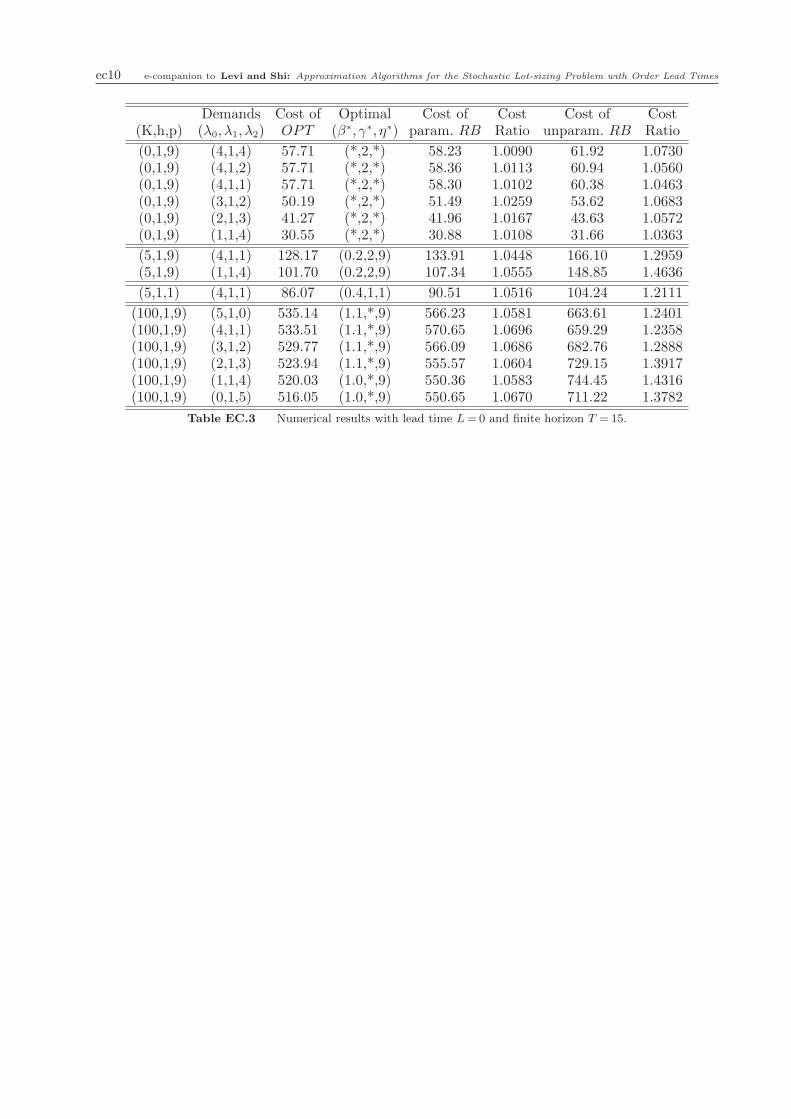
ec10 e-companion to Levi and Shi: Approximation Algorithms for the Stochastic Lot-sizing Problem with Order Lead Times
Demands Cost of Optimal Cost of Cost Cost of Cost(K,h,p) (λ0, λ1, λ2) OPT (β∗, γ∗, η∗) param. RB Ratio unparam. RB Ratio
(0,1,9) (4,1,4) 57.71 (*,2,*) 58.23 1.0090 61.92 1.0730(0,1,9) (4,1,2) 57.71 (*,2,*) 58.36 1.0113 60.94 1.0560(0,1,9) (4,1,1) 57.71 (*,2,*) 58.30 1.0102 60.38 1.0463(0,1,9) (3,1,2) 50.19 (*,2,*) 51.49 1.0259 53.62 1.0683(0,1,9) (2,1,3) 41.27 (*,2,*) 41.96 1.0167 43.63 1.0572(0,1,9) (1,1,4) 30.55 (*,2,*) 30.88 1.0108 31.66 1.0363
(5,1,9) (4,1,1) 128.17 (0.2,2,9) 133.91 1.0448 166.10 1.2959(5,1,9) (1,1,4) 101.70 (0.2,2,9) 107.34 1.0555 148.85 1.4636
(5,1,1) (4,1,1) 86.07 (0.4,1,1) 90.51 1.0516 104.24 1.2111
(100,1,9) (5,1,0) 535.14 (1.1,*,9) 566.23 1.0581 663.61 1.2401(100,1,9) (4,1,1) 533.51 (1.1,*,9) 570.65 1.0696 659.29 1.2358(100,1,9) (3,1,2) 529.77 (1.1,*,9) 566.09 1.0686 682.76 1.2888(100,1,9) (2,1,3) 523.94 (1.1,*,9) 555.57 1.0604 729.15 1.3917(100,1,9) (1,1,4) 520.03 (1.0,*,9) 550.36 1.0583 744.45 1.4316(100,1,9) (0,1,5) 516.05 (1.0,*,9) 550.65 1.0670 711.22 1.3782
Table EC.3 Numerical results with lead time L= 0 and finite horizon T = 15.