Approximation properties of certain operator-induced norms ...wainwrig/Papers/AmiWai11.pdf · 4 A.A. Amini, M.J. Wainwright / Journal of Approximation Theory ( ) – Hilbert sequence

Available online at www.sciencedirect.com

Journal of Approximation Theory ( ) –www.elsevier.com/locate/jat

Full length article

Approximation properties of certain operator-inducednorms on Hilbert spaces

Arash A. Aminib,∗, Martin J. Wainwrighta,b

a Department of Statistics, UC Berkeley, Berkeley, CA 94720, United Statesb Department of Electrical Engineering and Computer Sciences, UC Berkeley, Berkeley, CA 94720, United States

Received 7 June 2011; received in revised form 2 November 2011; accepted 7 November 2011

Communicated by Ding-Xuan Zhou

Abstract

We consider a class of operator-induced norms, acting as finite-dimensional surrogates to the L2 norm,and study their approximation properties over Hilbert subspaces of L2. The class includes, as a specialcase, the usual empirical norm encountered, for example, in the context of nonparametric regression in areproducing kernel Hilbert space (RKHS). Our results have implications to the analysis of M-estimatorsin models based on finite-dimensional linear approximation of functions, and also to some related packingproblems.c⃝ 2011 Elsevier Inc. All rights reserved.

Keywords: L2 approximation; Empirical norm; Quadratic functionals; Hilbert spaces with reproducing kernels; Analysisof M-estimators

1. Introduction

Given a probability measure P supported on a compact set X ⊂ Rd , consider the functionclass

L2(X ,P) :=

f : X → R | ‖ f ‖L2(X ,P) < ∞, (1)

∗ Corresponding author.E-mail addresses: [email protected], [email protected] (A.A. Amini), [email protected]

(M.J. Wainwright).

0021-9045/$ - see front matter c⃝ 2011 Elsevier Inc. All rights reserved.doi:10.1016/j.jat.2011.11.002

http://www.elsevier.com/locate/jat

http://dx.doi.org/10.1016/j.jat.2011.11.002

http://www.elsevier.com/locate/jat

mailto:[email protected]



http://dx.doi.org/10.1016/j.jat.2011.11.002

2 A.A. Amini, M.J. Wainwright / Journal of Approximation Theory ( ) –

where ‖ f ‖L2(X ,P) :=

X f 2(x) dP(x) is the usual L2 norm1 defined with respect to the

measure P. It is often of interest to construct approximations to this L2 norm that are “finite-dimensional” in nature, and to study the quality of approximation over the unit ball of someHilbert space H that is continuously embedded within L2. For example, in approximation theoryand mathematical statistics, a collection of n design points in X is often used to define a surrogatefor the L2 norm. In other settings, one is given some orthonormal basis of L2(X ,P), and definesan approximation based on the sum of squares of the first n (generalized) Fourier coefficients.For problems of this type, it is of interest to gain a precise understanding of the approximationaccuracy in terms of its dimension n and other problem parameters.

The goal of this paper is to study such questions in reasonable generality for the case of Hilbertspaces H. We let Φn : H → Rn denote a continuous linear operator on the Hilbert space, whichacts by mapping any f ∈ H to the n-vector

[Φn f ]1 [Φn f ]2 · · · [Φn f ]n

. This operator

defines the Φn-semi-norm

‖ f ‖Φn :=

n−i=1

[Φn f ]2i . (2)

In the sequel, with a minor abuse of terminology,2we refer to ‖ f ‖Φn as the Φn-norm of f . Ourgoal is to study how well ‖ f ‖Φn approximates ‖ f ‖L2 over the unit ball of H as a function of n,and other problem parameters. We provide a number of examples of the sampling operator Φnin Section 2.2. Since the dependence on the parameter n should be clear, we frequently omit thesubscript to simplify notation.

In order to measure the quality of approximation over H, we consider the quantity

RΦ(ε) := sup‖ f ‖

2L2 | f ∈ BH, ‖ f ‖

2Φ ≤ ε2, (3)

where BH := { f ∈ H | ‖ f ‖H ≤ 1} is the unit ball of H. The goal of this paper is to obtain sharpupper bounds on RΦ . As discussed in Appendix C, a relatively straightforward argument can beused to translate such upper bounds into lower bounds on the related quantity

T Φ(ε) := inf‖ f ‖

2Φ | f ∈ BH, ‖ f ‖

2L2 ≥ ε2. (4)

We also note that, for a complete picture of the relationship between the semi-norm ‖ · ‖Φ andthe L2 norm, one can also consider the related pair

TΦ(ε) := sup‖ f ‖

2Φ | f ∈ BH, ‖ f ‖

2L2 ≤ ε2, and (5a)

RΦ(ε) := inf‖ f ‖

2L2 | f ∈ BH, ‖ f ‖

2Φ ≥ ε2. (5b)

Our methods are also applicable to these quantities, but we limit our treatment to (RΦ, T Φ) soas to keep the contribution focused.

Certain special cases of linear operators Φ, and associated functionals have been studied inpast work. In the special case ε = 0, we have

RΦ(0) = sup‖ f ‖

2L2 | f ∈ BH,Φ( f ) = 0

,

1 We also use the simpler notation, L2, to refer to the space (1), with corresponding convention for its norm. Also, onecan take X to be a compact subset of any separable metric space and P a (regular) Borel measure.

2 This can be justified by identifying f and g if Φ f = Φg, i.e. considering the quotient H/ ker Φ.

A.A. Amini, M.J. Wainwright / Journal of Approximation Theory ( ) – 3

a quantity that corresponds to the squared diameter of BH ∩ Ker(Φ), measured in the L2-norm.Quantities of this type are standard in approximation theory (e.g., [4,10,11]), for instance in thecontext of Kolmogorov and Gelfand widths. Our primary interest in this paper is the more generalsetting with ε > 0, for which additional factors are involved in controlling RΦ(ε). In statistics,there is a literature on the case in which Φ is a sampling operator, which maps each functionf to a vector of n samples, and the norm ‖ · ‖Φ corresponds to the empirical L2-norm definedby these samples. When these samples are chosen randomly, then techniques from empiricalprocess theory [16] can be used to relate the two terms. As discussed in the sequel, our resultshave consequences for this setting of random sampling.

As an example of a problem in which an upper bound on RΦ is useful, let us consider ageneral linear inverse problem, in which the goal is to recover an estimate of the function f ∗

based on the noisy observations

yi = [Φ f ∗]i + wi , i = 1, . . . , n,

where {wi } are zero-mean noise variables, and f ∗∈ BH is unknown. An estimate f can be

obtained by solving a least-squares problem over the unit ball of the Hilbert space—that is, tosolve the convex program

f := arg minf ∈BH

n−i=1

(yi − [Φ f ]i )2.

For such estimators, there are fairly standard techniques for deriving upper bounds on the Φ-norm of the deviation f − f ∗. Our results in this paper on RΦ can then be used to translate thisto a corresponding upper bound on the L2-norm of the deviation f − f ∗, which is often a morenatural measure of performance.

As an example where the dual quantity T Φ might be helpful, consider the packing problemfor a subset D ⊂

12 BH of the Hilbert ball. Let M(ε; D, ‖ · ‖L2) be the ε-packing number of D

in ‖ · ‖L2 , i.e., the maximal number of function f1, . . . , fM ∈ D such that ‖ fi − f j‖L2 ≥ ε

for all i, j = 1, . . . ,M . Similarly, let M(ε; D, ‖ · ‖Φ) be the ε-packing number of D in ‖ · ‖Φ

norm. Now, suppose that for some fixed ε, T Φ(ε) > 0. Then, if we have a collection of functions{ f1, . . . , fM } which is an ε-packing of D in ‖ · ‖L2 , then the same collection will be a

T Φ(ε)-

packing of D in ‖ · ‖Φ . This implies the following useful relationship between packing numbers

M(ε; D, ‖ · ‖L2) ≤ M(

T Φ(ε); D, ‖ · ‖Φ).

The remainder of this paper is organized as follows. We begin in Section 2 with backgroundon the Hilbert space set-up, and provide various examples of the linear operators Φ to which ourresults apply. Section 3 contains the statement of our main result, and illustration of some of itsconsequences for different Hilbert spaces and linear operators. Finally, Section 4 is devoted tothe proofs of our results.

Notation: For any positive integer p, we use Sp+ to denote the cone of p × p positive semidefinite

matrices. For A, B ∈ Sp+, we write A ≽ B or B ≼ A to mean A − B ∈ Sp

+. For any squarematrix A, let λmin(A) and λmax(A) denote its minimal and maximal eigenvalues, respectively.We will use both

√A and A1/2 to denote the symmetric square root of A ∈ Sp

+. We will use{xk} = {xk}

∞

k=1 to denote a (countable) sequence of objects (e.g. real-numbers and functions).Occasionally we might denote an n-vector as {x1, . . . , xn}. The context will determine whetherthe elements between braces are ordered. The symbols ℓ2 = ℓ2(N) are used to denote the


Hilbert sequence space consisting of real-valued sequences equipped with the inner product⟨{xk}, {yk}⟩ℓ2 :=

∑∞

k=1 xi yi . The corresponding norm is denoted as ‖ · ‖ℓ2 .

2. Background

We begin with some background on the class of Hilbert spaces of interest in this paper andthen proceed to provide some examples of the sampling operators of interest.

2.1. Hilbert spaces

We consider a class of Hilbert function spaces contained within L2(X ,P), and defined asfollows. Let {ψk}

∞

k=1 be an orthonormal sequence (not necessarily a basis) in L2(X ,P) and letσ1 ≥ σ2 ≥ σ3 ≥ · · · > 0 be a sequence of positive weights decreasing to zero. Given these twoingredients, we can consider the class of functions

H :=

f ∈ L2(X ,P) | f =

∞−k=1

√σkαkψk, for some {αk}

∞

k=1 ∈ ℓ2(N)

, (6)

where the series in (6) is assumed to converge in L2. (The series converges since∑∞

k=1(√σkαk)

2≤ σ1‖{αk}‖ℓ2 < ∞.) We refer to the sequence {αk}

∞

k=1 ∈ ℓ2 as therepresentative of f . Note that this representation is unique due to σk being strictly positive for allk ∈ N.

If f and g are two members of H, say with associated representatives α = {αk}∞

k=1 andβ = {βk}

∞

k=1, then we can define the inner product

⟨ f, g⟩H :=

∞−k=1

αkβk = ⟨α, β⟩ℓ2 . (7)

With this choice of inner product, it can be verified that the space H is a Hilbert space. (In fact,H inherits all the required properties directly from ℓ2.) For future reference, we note that for twofunctions f, g ∈ H with associated representatives α, β ∈ ℓ2, their L2-based inner product isgiven by3

⟨ f, g⟩L2 =∑

∞

k=1 σkαkβk .We note that each ψk is in H, as it is represented by a sequence with a single nonzero element,

namely, the k-th element which is equal to σ−1/2k . It follows from (7) that ⟨

√σkψk,

√σ jψ j ⟩H =

δk j . That is, {√σkψk} is an orthonormal sequence in H. Now, let f ∈ H be represented by

α ∈ ℓ2. We claim that the series in (6) also converges in H norm. In particular,∑N

k=1√σkαkψk

is in H, as it is represented by the sequence {α1, . . . , αN , 0, 0, . . .} ∈ ℓ2. It follows from (7) that‖ f −

∑Nk=1

√σkαkψk‖H =

∑∞

k=N+1 α2k which converges to 0 as N → ∞. Thus, {

√σkψk} is in

fact an orthonormal basis for H.We now turn to a special case of particular importance to us, namely the reproducing

kernel Hilbert space (RKHS) of a continuous kernel. Consider a symmetric bivariate functionK : X ×X → R, where X ⊂ Rd is compact.4 Furthermore, assume K to be positive semidefiniteand continuous. Consider the integral operator IK mapping a function f ∈ L2 to the function

3 In particular, for f ∈ H, ‖ f ‖L2 ≤√σ1‖ f ‖H which shows that the inclusion H ⊂ L2 is continuous.

4 Also assume that P assign positive mass to every open Borel subset of X .


IK f :=

K(·, y) f (y)dP(y). As a consequence of Mercer’s theorem [13,6], IK is a compactoperator from L2 to C(X ), the space of continuous functions on X equipped with the uniformnorm.5 Let {σk} be the sequence of nonzero eigenvalues of IK, which are positive, can be orderedin nonincreasing order and converge to zero. Let {ψk} be the corresponding eigenfunctions whichare continuous and can be taken to be orthonormal in L2. With these ingredients, the space Hdefined in Eq. (6) is the RKHS of the kernel function K. This can be verified as follows.

As another consequence of the Mercer’s theorem, K has the decomposition

K(x, y) :=

∞−k=1

σkψk(x)ψk(y) (8)

where the convergence is absolute and uniform (in x and y). In particular, for any fixed y ∈ X ,the sequence {

√σkψk(y)} is in ℓ2. (In fact,

∑∞

k=1(√σkψk(y))2 = K(y, y) < ∞.) Hence, K(·, y)

is in H, as defined in (6), with representative {√σkψk(y)}. Furthermore, it can be verified that the

convergence in (6) can be taken to be also pointwise.6 To be more specific, for any f ∈ H withrepresentative {αk}

∞

k=1 ∈ ℓ2, we have f (y) =∑

∞

k=1√σkαkψk(y), for all y ∈ X . Consequently,

by definition of the inner product (7), we have

⟨ f,K(·, y)⟩H =

∞−k=1

αk√σkψk(y) = f (y),

so that K(·, y) acts as the representer of evaluation. This argument shows that for any fixedy ∈ X , the linear functional on H given by f → f (y) is bounded, since we have

| f (y)| = |⟨ f,K(·, y)⟩H| ≤ ‖ f ‖H‖K(·, y)‖H,

hence H is indeed the RKHS of the kernel K. This fact plays an important role in the sequel,since some of the linear operators that we consider involve pointwise evaluation.

A comment regarding the scope: our general results hold for the basic setting introduced inEq. (6). For those examples that involve pointwise evaluation, we assume the more refined caseof the RKHS described above.

2.2. Linear operators, semi-norms and examples

Let Φ : H → Rn be a continuous linear operator, with co-ordinates [Φ f ]i for i = 1, 2, . . . , n.It defines the (semi)-inner product

⟨ f, g⟩Φ := ⟨Φ f,Φg⟩Rn , (9)

which induces the semi-norm ‖ · ‖Φ . By the Riesz representation theorem, for each i = 1, . . . , n,there is a function ϕi ∈ H such that [Φ f ]i = ⟨ϕi , f ⟩H for any f ∈ H.Let us illustrate the preceding definitions with some examples.

Example 1 (Generalized Fourier Truncation). Recall the orthonormal basis {ψi }∞

i=1 underlyingthe Hilbert space. Consider the linear operator Tψn

1: H → Rn with coordinates

[Tψn1

f ]i := ⟨ψi , f ⟩L2 , for i = 1, 2, . . . , n. (10)

5 In fact, IK is well defined over L1⊃ L2 and the conclusions about IK hold as a operator from L1 to C(X ).

6 The convergence is actually even stronger, namely it is absolute and uniform, as can be seen by noting that∑mk=n+1 |αk

√σkψk (y)| ≤ (

∑mk=n+1 α

2k )

1/2(∑m

k=n+1 σkψ2k (y))

1/2≤ (

∑mk=n+1 α

2k )

1/2 maxy∈X K(y, y).


We refer to this operator as the (generalized) Fourier truncation operator, since it acts bytruncating the (generalized) Fourier representation of f to its first n co-ordinates. More precisely,by construction, if f =

∑∞

k=1√σkαkψk , then

[Φ f ]i =√σiαi , for i = 1, 2, . . . , n. (11)

By definition of the Hilbert inner product, we have αi =√σi ⟨ψi , f ⟩H, so that we can write

[Φ f ]i = ⟨ϕi , f ⟩H, where ϕi := σiψi . �

Example 2 (Domain Sampling). A collection xn1 := {x1, . . . , xn} of points in the domain X can

be used to define the (scaled) sampling operator Sxn1

: H → Rn via

Sxn1

f := n−1/2 f (x1) · · · f (xn), for f ∈ H. (12)

As previously discussed, when H is a reproducing kernel Hilbert space (with kernel K), the(scaled) evaluation functional f → n−1/2 f (xi ) is bounded, and its Riesz representation is givenby the function ϕi = n−1/2K(·, xi ). �

Example 3 (Weighted Domain Sampling). Consider the setting of the previous example. A slightvariation on the sampling operator (12) is obtained by adding some weights to the samples

Wxn1 ,w

n1

f := n−1/2 w1 f (x1) · · · wn f (xn), for f ∈ H (13)

where wn1 = (w1, . . . , wn) is chosen such that

∑nk=1w

2k = 1. Clearly, we have ϕi =

n−1/2wi K(·, xi ).As an example of how this might arise, consider approximating f (t) by

∑nk=1 f (xk)Gn(t, xk)

where {Gn(·, xk)} is a collection of functions in L2(X ,P) such that ⟨Gn(·, xk),Gn(·, x j )⟩L2 =

n−1w2kδk j . Proper choices of {Gn(·, xi )} might produce better approximations to the L2 norm

in the cases where one insists on choosing elements of xn1 to be uniformly spaced, while P

in (1) is not a uniform distribution. Another slightly different but closely related case is whenone approximates f 2(t) over X = [0, 1], by say n−1∑n−1

k=1 f 2(xk)W (n(t − xk)) for somefunction W : [−1, 1] → R+ and xk = k/n. Again, non-uniform weights are obtained whenP is nonuniform. �

3. Main result and some consequences

We now turn to the statement of our main result, and the development of some of itsconsequences for various models.

3.1. General upper bounds on RΦ(ε)

We start with upper bounds on RΦ(ε) which was defined previously in (3). Our bounds arestated in terms of a real-valued function defined as follows: for matrices D,M ∈ Sp

+,

L(t,M, D) := maxλmax

D − t

√DM

√D, 0, for t ≥ 0. (14)

Here√

D denotes the matrix square root, valid for positive semidefinite matrices.The upper bounds on RΦ(ε) involve principal submatrices of certain infinite-dimensional

matrices – or equivalently linear operators on ℓ2(N) – that we define here. Let Ψ be the infinite-dimensional matrix with entries

[Ψ] jk := ⟨ψ j , ψk⟩Φ, for j, k = 1, 2, . . . , (15)


and let Σ = diag{σ1, σ2, . . . , } be a diagonal operator. For any p = 1, 2, . . . , we use Ψp andΨp to denote the principal submatrices of Ψ on rows and columns indexed by {1, 2, . . . , p} and{p + 1, p + 2, . . .}, respectively. A similar notation will be used to denote submatrices of Σ.

Theorem 1. For all ε ≥ 0, we have:

RΦ(ε) ≤ infp∈N

inft≥0

L(t,Ψp,Σp)+ t

ε +

λmax(Σ

1/2p ΨpΣ 1/2p )2

+ σp+1

. (16)

Moreover, for any p ∈ N such that λmin(Ψp) > 0, we have

RΦ(ε) ≤

1 −

σp+1

σ1

1

λmin(Ψp)

ε +

λmax(Σ

1/2p ΨpΣ 1/2p )2

+ σp+1. (17)

Remark (a): These bounds cannot be improved in general. This is most easily seen in the specialcase ε = 0. Setting p = n, bound (17) implies that RΦ(0) ≤ σn+1 whenever Ψn is strictlypositive definite and Ψn = 0. This bound is sharp in a “minimax sense”, meaning that equalityholds if we take the infimum over all bounded linear operators Φ : H → Rn . In particular, it isstraightforward to show that

infΦ:H→RnΦ surjective

RΦ(0) = infΦ:H→RnΦ surjective

supf ∈BH

‖ f ‖

2L2 | Φ f = 0

= σn+1, (18)

and moreover, this infimum is in fact achieved by some linear operator. Such results are knownfrom the general theory of n-widths for Hilbert spaces (e.g., see Chapter IV in [10] and Chapter 3of [5]).

In the more general setting of ε > 0, there are operators for which the bound (17) is met withequality. As a simple illustration, recall the (generalized) Fourier truncation operator Tψn

1from

Example 1. First, it can be verified that ⟨ψk, ψ j ⟩Tψn1

= δ jk for j, k ≤ n and ⟨ψk, ψ j ⟩Tψn1

= 0

otherwise. Taking p = n, we have Ψn = In , that is, the n-by-n identity matrix, and Ψn = 0.Setting p = n in (17), it follows that for ε2

≤ σ1,

RTψn1(ε) ≤

1 −

σn+1

σ1

ε2

+ σn+1. (19)

As shown in Appendix E, the bound (19) in fact holds with equality. In other words, the boundsof Theorem 1 are tight in this case. Also, note that (19) implies RTψn

1(0) ≤ σn+1 showing that the

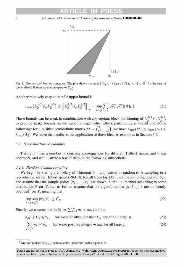
(generalized) Fourier truncation operator achieves the minimax bound of (18). Fig. 1 provides ageometric interpretation of these results.

Remark (b): In general, it might be difficult to obtain a bound on the quantity λmax(Σ1/2p ΨpΣ 1/2p )

as it involves the infinite dimensional matrix Ψp. One may obtain a simple (although not usuallysharp) bound on this quantity by noting that for a positive semidefinite matrix, the maximaleigenvalue is bounded by the trace, that is,

λmaxΣ 1/2p ΨpΣ 1/2p

≤ trΣ 1/2p ΨpΣ 1/2p

=

−k>p

σk[Ψ]kk . (20)


Fig. 1. Geometry of Fourier truncation. The plot shows the set {(‖ f ‖L2 , ‖ f ‖Φ) : ‖ f ‖H ≤ 1} ⊂ R2 for the case of(generalized) Fourier truncation operator Tψn

1.

Another relatively easy-to-handle upper bound is


≤

Σ 1/2p ΨpΣ 1/2p

∞

= supk>p

−r>p

√σk

√σr |[Ψ]kr |. (21)

These bounds can be used, in combination with appropriate block partitioning of Σ 1/2p ΨpΣ 1/2p ,to provide sharp bounds on the maximal eigenvalue. Block partitioning is useful due to the

following: for a positive semidefinite matrix M =

A1 CCT A2

, we have λmax(M) ≤ λmax(A1) +

λmax(A2). We leave the details on the application of these ideas to examples in Section 3.2.

3.2. Some illustrative examples

Theorem 1 has a number of concrete consequences for different Hilbert spaces and linearoperators, and we illustrate a few of them in the following subsections.

3.2.1. Random domain samplingWe begin by stating a corollary of Theorem 1 in application to random time sampling in a

reproducing kernel Hilbert space (RKHS). Recall from Eq. (12) the time sampling operator Sxn1,

and assume that the sample points {x1, . . . , xn} are drawn in an i.i.d. manner according to somedistribution P on X . Let us further assume that the eigenfunctions ψk, k ≥ 1 are uniformlybounded7 on X , meaning that

supk≥1

supx∈X

|ψk(x)| ≤ Cψ . (22)

Finally, we assume that ‖σ‖1 :=∑

∞

k=1 σk < ∞, and that

σpk ≤ Cσσkσp, for some positive constant Cσ and for all large p, (23)−k>pm

σk ≤ σp, for some positive integer m and for all large p. (24)

7 One can replace supx∈X with essential supremum with respect to P.


In each case, for all large p means for all p ≥ p0 for some constant positive integer p0. Let mσ

be the smallest m for which (24) holds. These conditions on {σk} are satisfied, for example, forboth a polynomial decay σk = O(k−α) with α > 1 and an exponential decay σk = O(ρk) withρ ∈ (0, 1). In particular, for the polynomial decay, using the tail bound (B.1) in Appendix B,we can take mσ = ⌈

αα−1⌉ to satisfy (24). For the exponential decay, we can take mσ = 1 for

ρ ∈ (0, 12 ] and mσ = 2 for ρ ∈ ( 1

2 , 1) to satisfy (24).Define the function

Gn(ε) :=1

√n

∞−j=1

min{σ j , ε2}, (25)

as well as the critical radius

rn := inf{ε > 0 : Gn(ε) ≤ ε2}. (26)

With these definitions, we have the following result:

Corollary 1. Suppose that rn > 0 and 64C2ψmσ r2

n log(2nr2n ) ≤ 1. Then for any ε2

∈ [r2n , σ1),

we have

P

RSxn1(ε) > (Cψ + Cσ )ε2

≤ 2 exp

−

1

64C2ψr2

n

, (27)

where Cψ := 2(1 + Cψ )2 and Cσ := 3(1 + C−1ψ )Cσ‖σ‖1 + 1.

We provide the proof of this corollary in Appendix A. As a concrete example, consider apolynomial decay σk = O(k−α) for α > 1, which satisfies assumptions on {σk}. Using the tailbound (B.1) in Appendix B, one can verify that r2

n = O(n−α/(α+1)). Note that, in this case,

r2n log(2nr2

n ) = O

n−αα+1 log n

1α+1

= O

n−

αα+1 log n

→ 0, n → ∞.

Hence the conditions of Corollary 1 are met for sufficiently large n. It follows that for someconstants C1, C2 and C3, we have

RSxn1

C1n−

α2(α+1)

≤ C2n−

αα+1

with probability 1 − 2 exp(−C3nαα+1 ) for sufficiently large n.

As noted previously, for this particular case of random time sampling, different techniquesfrom empirical process theory (e.g., [16,3,7]) can be used to control the quantity RSxn

1(ε). As one

concrete instance of such a result, when functions in the RKHS are uniformly bounded, Lemma 7of Raskutti et al. [12] with t = rn implies that

PRSxn

1(rn) > c0r2

n

≤ c1 exp

−c2nr2

n

(28)

for some constants ci , i = 1, 2, 3, independent of sample size n, but depending on bounds on thefunction class. The result (28) provides a qualitatively similar guarantee to Corollary 1, with themain difference being the factor nr2

n in the exponent, as opposed to the term 1/r2n in the bound

(27). For kernels with the polynomial decay σk = O(k−α) for some α > 1, it can be verified

that nr2n ≍ n

1α+1 , whereas 1

r2n

= nαα+1 . Since α > 1, we thus see that Corollary 1 provides


guarantees with a faster probabilistic rate. In addition, results of the type (28) are proved usingtechniques rather different than the current paper, including concentration bounds for empiricalprocesses [8,3,16] and the Ledoux–Talagrand contraction inequality (e.g., [8]). The function (25)again plays a role in this result, in particular via its connection to the Rademacher complexity ofkernel classes [9].

As pointed out by a helpful reviewer, it would be desirable to weaken or remove the uniformboundedness condition (22) on the eigenfunctions. We suspect that extensions of this type mightbe possible when the random variables ψk(x) satisfy some type of tail condition (e.g., a boundon a suitable Orlicz norm [17]). We note that arguments of this type are used in the empiricalprocess theory literature (e.g., [1]). At this time, we do not have a simple argument for our settingof RKHS’s and Theorem 1.

3.2.2. Sobolev kernel

Consider the kernel K(x, y) = min(x, y) defined on X 2 where X = [0, 1] and let P beuniform (i.e., the Lebesgue measure restricted to [0, 1]). The corresponding RKHS is of Sobolevtype and can be expressed as

f ∈ L2(X ,P) | f is absolutely continuous, f (0) = 0 and f ′∈ L2(X ,P)

.

Also consider a uniform domain sampling operator Sxn1, that is, that of (12) with xi = i/n, i ≤ n.

This setting has the benefit that many interesting quantities can be computed explicitly, whilealso having some practical appeal. The following can be shown about the eigen-decompositionof the integral operator IK introduced in Section 2,

σk =

(2k − 1)π

2

−2

, ψk(x) =√

2 sinσ

−1/2k x

, k = 1, 2, . . . .

In particular, the eigenvalues decay as σk = O(k−2).To compute the Ψ, we write

[Ψ]kr = ⟨ψk, ψr ⟩Φ =1n

n−ℓ=1

cos

(k − r)ℓπ

n− cos

(k + r − 1)ℓπn

. (29)

We note that Ψ is periodic in k and r with period 2n. It is easily verified that∑nℓ=1 cos(qℓπ/n)

is equal to −1 for odd values of q and zero for even values, other than q = 0,±2n,±4n, . . . . Itfollows that

[Ψ]kr =

1 +

1n

if k − r = 0,

−1 −1n

if k + r = 2n + 1

1n(−1)k−r otherwise,

(30)

for 1 ≤ k, r ≤ 2n. Letting Is ∈ Rn be the vector with entries, (Is) j = (−1) j+1, j ≤ n, weobserve that Ψn = In +

1n IsIT

s . It follows that λmin(Ψn) = 1. It remains to bound the terms in(17) involving the infinite sub-block Ψn .


a b

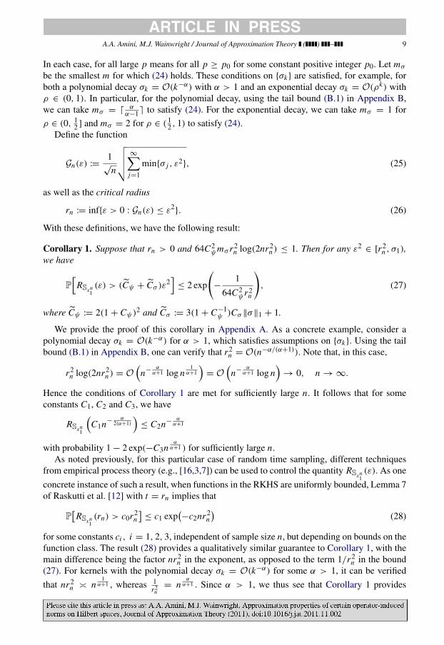
Fig. 2. Sparse periodic Ψ matrices. Display (a) is a plot of the N -by-N leading principal submatrix of Ψ for the Sobolevkernel (s, t) → min{s, t}. Here n = 9 and N = 6n; the period is 2n = 18. Display (b) is the same plot for a Fourier-typekernel. The plots exhibit sparse periodic patterns as defined in Section 3.2.2.

The Ψ matrix of this example, given by (30), shares certain properties with the Ψ obtainedin other situations involving periodic eigenfunctions {ψk}. We abstract away these properties byintroducing a class of periodic Ψ matrices. We call Ψn a sparse periodic matrix, if each row(or column) is periodic and in each period only a vanishing fraction of elements are large. Moreprecisely, Ψn is sparse periodic if there exist positive integers γ and η, and nonnegative constantsc1 and c2, all independent of n, such that each row of Ψn is periodic with period γ n and for anyrow k, there exists a subset of elements Sk = {ℓ1, . . . , ℓη} ⊂ {1, . . . , γ n} such that

|[Ψ]k,n+r | ≤ c1, r ∈ Sk, (31a)

|[Ψ]k,n+r | ≤ c2n−1, r ∈ {1, . . . , γ n} \ Sk, (31b)

The elements of Sk could depend on k, but the cardinality of this set should be the constantη, independent of k and n. Also, note that we are indexing rows and columns of Ψn by{n + 1, n + 2, . . .}; in particular, k ≥ n + 1. Fig. 2 illustrates some examples. For this class,we have the following whose proof can be found in Appendix B.

Lemma 1. Assume that Ψn is sparse periodic as defined above and σk = O(k−α) for someα ≥ 2. Then:

(a) For α > 2, λmaxΣ 1/2n ΨnΣ 1/2n

= O(n−α) as n → ∞,

(b) For α = 2, λmaxΣ 1/2n ΨnΣ 1/2n

= O(n−2 log n) as n → ∞.

In particular, Eq. (30) implies that Ψn is sparse periodic with parameters γ = 2, η = 2, c1 = 2and c2 = 1. Hence, part (b) of Lemma 1 applies. Now, we can use (17) with p = n to obtain

RSxn1(ε) ≤ 2ε2

+ On−2 log n

(32)

where we have also used (a + b)2 ≤ 2a2+ 2b2.


3.2.3. Fourier-type kernelsIn this example, we consider an RKHS of functions on X = [0, 1] ⊂ R, generated by a

Fourier-type kernel defined as K(x, y) := κ(x − y), x, y ∈ [0, 1], where

κ(x) = ζ0 +

∞−k=1

2ζk cos(2πkx), x ∈ [−1, 1]. (33)

We assume that (ζk) is a R+-valued nonincreasing sequence in ℓ1, i.e.∑

k ζk < ∞. Thus, thetrigonometric series in (33) is absolutely (and uniformly) convergent. As for the operator Φ,we consider the uniform time sampling operator Sxn

1, as in the previous example. That is, the

operator defined in (12) with xi = i/n, i ≤ n. We take P to be uniform.This setting again has the benefit of being simple enough to allow for explicit computations

while also practically important. One can argue that the eigen-decomposition of the kernelintegral operator is given by

ψ1 = ψ(c)0 , ψ2k = ψ

(c)k , ψ2k+1 = ψ

(s)k , k ≥ 1 (34)

σ1 = ζ0, σ2k = ζk, σ2k+1 = ζk, k ≥ 1 (35)

where ψ (c)0 (x) := 1, ψ (c)k (x) :=√

2 cos(2πkx) and ψ (s)k (t) :=√

2 sin(2πkx) for k ≥ 1.For any integer k, let ((k))n denote k modulo n. Also, let k → δk be the function defined

over integers which is 1 at k = 0 and zero elsewhere. Let ι :=√

−1. Using the identityn−1∑n

ℓ=1 exp(ι2πkℓ/n) = δ((k))n , one obtains the following,

⟨ψ(c)k , ψ

(c)j ⟩Φ =

δ((k− j))n + δ((k+ j))n

1√

2

δk+δ j, (36a)

⟨ψ(s)k , ψ

(s)j ⟩Φ = δ((k− j))n − δ((k+ j))n , (36b)

⟨ψ(c)k , ψ

(s)j ⟩Φ = 0, valid for all j, k ≥ 0. (36c)

It follows that Ψn = In if n is odd and Ψn = diag{1, 1, . . . , 1, 2} if n is even. In particular,λmin(Ψn) = 1 for all n ≥ 1. It is also clear that the principal submatrix of Ψ on indices {2, 3, . . .}has periodic rows and columns with period 2n. If follows that Ψn is sparse periodic as defined inSection 3.2.2 with parameters γ = 2, η = 2, c1 = 2 and c2 = 0.

Suppose for example that the eigenvalues decay polynomially, say as ζk = O(k−α) for α > 2.Then, applying (17) with p = n, in combination with Lemma 1 part (a), we get

RSxn1(ε) ≤ 2ε2

+ O(n−α). (37)

As another example, consider the exponential decay ζk = ρk, k ≥ 1 for some ρ ∈ (0, 1), whichcorresponds to the Poisson kernel. In this case, the tail sum of {σk} decays as the sequence itself,namely,

∑k>n σk ≤ 2

∑k>n ρ

k=

2ρ1−ρ

ρk . Hence, we can simply use the trace bound (20)together with (17) to obtain

RSxn1(ε) ≤ 2ε2

+ O(ρn). (38)

4. Proof of Theorem 1

We now turn to the proof of our main theorem. Recall from Section 2.1 the correspondencebetween any f ∈ H and a sequence α ∈ ℓ2; also, recall the diagonal operator Σ : ℓ2 → ℓ2


defined by the matrix diag{σ1, σ2, . . .}. Using the definition of (15) of the Ψ matrix, we have

‖ f ‖2Φ = ⟨α,Σ 1/2ΨΣ 1/2α⟩ℓ2 .

By definition (6) of the Hilbert space H, we have ‖ f ‖2H =

∑∞

k=1 α2k and ‖ f ‖

2L2 =

∑k σkα

2k .

Letting Bℓ2 =α ∈ ℓ2 | ‖α‖ℓ2 ≤ 1

be the unit ball in ℓ2, we conclude that RΦ can be written

as

RΦ(ε) = supα∈Bℓ2

Q2(α) | QΦ(α) ≤ ε2, (39)

where we have defined the quadratic functionals

Q2(α) := ⟨α,Σα⟩ℓ2 , and QΦ(α) := ⟨α,Σ 1/2ΨΣ 1/2α⟩ℓ2 . (40)

Also let us define the symmetric bilinear form

BΦ(α, β) := ⟨α,Σ 1/2ΨΣ 1/2β⟩ℓ2 , α, β ∈ ℓ2, (41)

whose diagonal is BΦ(α, α) = QΦ(α).We now upper bound RΦ(ε) using a truncation argument. Define the set

C := {α ∈ Bℓ2 | QΦ(α) ≤ ε2}, (42)

corresponding to the feasible set for the optimization problem (39). For each integer p =

1, 2, . . . , consider the following truncated sequence spaces

T p :=α ∈ ℓ2 | αi = 0, for all i > p

, and

T ⊥p :=

α ∈ ℓ2 | αi = 0, for all i = 1, 2, . . . p

.

Note that ℓ2 is the direct sum of T p and T ⊥p . Consequently, any fixed α ∈ C can be decomposed

as α = ξ + γ for some (unique) ξ ∈ T p and γ ∈ T ⊥p . Since Σ is a diagonal operator, we have

Q2(α) = Q2(ξ)+ Q2(γ ).

Moreover, since any α ∈ C is feasible for the optimization problem (39), we have

QΦ(α) = QΦ(ξ)+ 2BΦ(ξ, γ )+ QΦ(γ ) ≤ ε2. (43)

Note that since γ ∈ T ⊥p , it can be written as γ = (0p, c), where 0p is a vector of p zeros, and

c = (c1, c2, . . .) ∈ ℓ2. Similarly, we can write ξ = (x, 0) where x ∈ Rp. Then, each of theterms QΦ(ξ), BΦ(ξ, γ ), QΦ(γ ) can be expressed in terms of block partitions of Σ 1/2ΨΣ 1/2.For example,

QΦ(ξ) = ⟨x, Ax⟩Rp , QΦ(γ ) = ⟨y, Dy⟩ℓ2 , (44)

where A := Σ 1/2p ΨpΣ

1/2p and D := Σ 1/2p ΨpΣ 1/2p , in correspondence with the block partitioning

notation of Appendix F. We now apply inequality (F.2) derived in Appendix F. Fix someρ2

∈ (0, 1) and take

κ2:= ρ2λmax(Σ

1/2p ΨpΣ 1/2p ), (45)


so that condition (F.5) is satisfied. Then, (F.2) implies

QΦ(ξ)+ 2BΦ(ξ, γ )+ QΦ(γ ) ≥ ρ2 QΦ(ξ)−κ2

1 − ρ2 ‖γ ‖22. (46)

Combining (43) and (46), we obtain

QΦ(ξ) ≤ε2

ρ2 +λmax(Σ

1/2p ΨpΣ 1/2p )

1 − ρ2 ‖γ ‖22. (47)

We further note that ‖γ ‖22 ≤ ‖γ ‖

22 + ‖ξ‖2

2 = ‖α‖22 ≤ 1. It follows that

QΦ(ξ) ≤ε2, whereε2:=

ε2

ρ2 +λmax(Σ

1/2p ΨpΣ 1/2p )

1 − ρ2 . (48)

Let us defineC := {ξ ∈ Bℓ2 ∩ T p | QΦ(ξ) ≤ε2}. (49)

Then, our arguments so far show that for α ∈ C,

Q2(α) = Q2(ξ)+ Q2(γ ) ≤ supξ∈C Q2(ξ)

Sp

+ supγ∈Bℓ2∩T ⊥

p

Q2(γ ) S⊥

p

. (50)

Taking the supremum over α ∈ C yields the upper bound

RΦ(ε) ≤ Sp + S⊥p .

It remains to bound each of the two terms on the right-hand side. Beginning with the term S⊥p

and recalling the decomposition γ = (0p, c), we have Q2(γ ) =∑

∞

k=1 σk+pc2k , from which it

follows that

S⊥p = sup

∞−

k=1

σk+pc2k |

∞−k=1

c2k ≤ 1

= σp+1,

since {σk}∞

k=1 is a nonincreasing sequence by assumption.We now control the term Sp. Recalling the decomposition ξ = (x, 0) where x ∈ Rp, we have

Sp = supξ∈C Q2(ξ) = sup

⟨x,Σpx⟩ : ⟨x, x⟩ ≤ 1, ⟨x,Σ 1/2

p ΨpΣ1/2p x⟩ ≤ε2

= sup⟨x,x⟩≤1

inft≥0

⟨x,Σpx⟩ + t

ε2− ⟨x,Σ 1/2

p ΨpΣ1/2p x⟩

(a)≤ inf

t≥0

sup

⟨x,x⟩≤1⟨x,Σ 1/2

p (Ip − tΨp)Σ1/2p x⟩ + tε2

where inequality (a) follows by Lagrange (weak) duality. It is not hard to see that for anysymmetric matrix M , one has

sup⟨x,Mx⟩ : ⟨x, x⟩ ≤ 1

= max

0, λmax(M)

.


a b

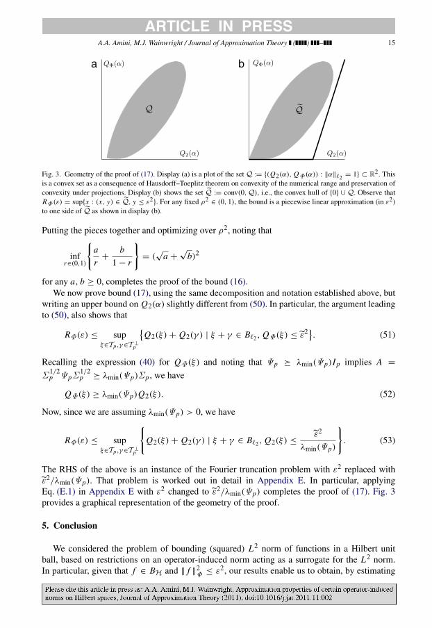
Fig. 3. Geometry of the proof of (17). Display (a) is a plot of the set Q := {(Q2(α), QΦ(α)) : ‖α‖ℓ2 = 1} ⊂ R2. Thisis a convex set as a consequence of Hausdorff–Toeplitz theorem on convexity of the numerical range and preservation ofconvexity under projections. Display (b) shows the set Q := conv(0,Q), i.e., the convex hull of {0} ∪ Q. Observe thatRΦ(ε) = sup{x : (x, y) ∈ Q, y ≤ ε2

}. For any fixed ρ2∈ (0, 1), the bound is a piecewise linear approximation (in ε2)

to one side of Q as shown in display (b).

Putting the pieces together and optimizing over ρ2, noting that

infr∈(0,1)

a

r+

b

1 − r

= (

√a +

√b)2

for any a, b ≥ 0, completes the proof of the bound (16).We now prove bound (17), using the same decomposition and notation established above, but

writing an upper bound on Q2(α) slightly different from (50). In particular, the argument leadingto (50), also shows that

RΦ(ε) ≤ supξ∈T p,γ∈T ⊥

p

Q2(ξ)+ Q2(γ ) | ξ + γ ∈ Bℓ2 , QΦ(ξ) ≤ε2. (51)

Recalling the expression (40) for QΦ(ξ) and noting that Ψp ≽ λmin(Ψp)Ip implies A =

Σ 1/2p ΨpΣ

1/2p ≽ λmin(Ψp)Σp, we have

QΦ(ξ) ≥ λmin(Ψp)Q2(ξ). (52)

Now, since we are assuming λmin(Ψp) > 0, we have

RΦ(ε) ≤ supξ∈T p,γ∈T ⊥

p

Q2(ξ)+ Q2(γ ) | ξ + γ ∈ Bℓ2 , Q2(ξ) ≤

ε2

λmin(Ψp)

. (53)

The RHS of the above is an instance of the Fourier truncation problem with ε2 replaced withε2/λmin(Ψp). That problem is worked out in detail in Appendix E. In particular, applyingEq. (E.1) in Appendix E with ε2 changed toε2/λmin(Ψp) completes the proof of (17). Fig. 3provides a graphical representation of the geometry of the proof.

5. Conclusion

We considered the problem of bounding (squared) L2 norm of functions in a Hilbert unitball, based on restrictions on an operator-induced norm acting as a surrogate for the L2 norm.In particular, given that f ∈ BH and ‖ f ‖

2Φ ≤ ε2, our results enable us to obtain, by estimating


norms of certain finite and infinite dimensional matrices, inequalities of the form

‖ f ‖2L2 ≤ c1ε

2+ hΦ,H(σn)

where {σn} are the eigenvalues of the operator embedding H in L2, hΦ,H(·) is an increasingfunction (depending on Φ and H) and c1 ≥ 1 is some constant. We considered examples ofoperators Φ (uniform time sampling and Fourier truncation) and Hilbert spaces H (Sobolev,Fourier-type RKHSs) and showed that it is possible to obtain optimal scaling hΦ,H(σn) = O(σn)

in most of those cases. We also considered random time sampling, under polynomial eigen-decayσn = O(n−α), and effectively showed that hΦ,H(σn) = O(n−α/(α+1)) (for ε small enough), withhigh probability as n → ∞. This last result complements those on related quantities obtained bytechniques from empirical process theory, and we conjecture it to be sharp.

Acknowledgments

AA and MJW were partially supported by NSF Grant CAREER-CCF-0545862 and AFOSRGrant 09NL184.

Appendix A. Analysis of random time sampling

This section is devoted to the proof of Corollary 1 on random time sampling in reproducingkernel Hilbert spaces. The proof is based on an auxiliary result, which we begin by stating. Fixsome positive integer m and define

ν(ε) = ν(ε; m) := inf

p :

−k>pm

σk ≤ ε2. (A.1)

With this notation, we have

Lemma 2. Assume ε2 < σ1 and 32C2ψmν(ε) log ν(ε) ≤ n. Then,

P

RSxn1(ε) > Cψε2

+ Cσσν(ε) ≤ 2 exp

−

1

32C2ψ

n

ν(ε)

. (A.2)

We prove this claim in Appendix A.2.

A.1. Proof of Corollary 1

To apply the lemma, recall that we assume that there exists m such that for all (large) p, onehas −

k>pm

σk ≤ σp (A.3)

and we let mσ be the smallest such m. We define

µ(ε) := inf

p : σp ≤ ε2, (A.4)

and note that by (A.3), we have ν(ε; mσ ) ≤ µ(ε). Then, Lemma 2 states that as long as ε2 < σ1and 32C2

ψmσµ(ε) logµ(ε) ≤ n, we have


P

RSxn1(ε) > (Cψ + Cσ )ε2

≤ 2 exp

−

1

32C2ψ

n

µ(ε)

. (A.5)

Now by the definition of µ(ε), we have σ j > ε2 for j < µ(ε), and hence

G 2n(ε) ≥

1n

−j<µ(ε)

min{σ j , ε2} =

µ(ε)− 1n

ε2≥µ(ε)

2nε2,

since µ(ε) ≥ 2 when ε2 < σ1. One can argue that ε → Gn(ε)/ε is nonincreasing. It followsfrom definition (26) that for ε ≥ rn , we have

µ(ε) ≤ 2n

G(ε)ε

2

≤ 2n

G(rn)

rn

2

≤ 2nr2n ,

which completes the proof of Corollary 1.

A.2. Proof of Lemma 2

For ξ ∈ Rp, let ξ⊗ξ be the rank-one operator on Rp given by η → ⟨ξ, , η⟩2ξ . For an operatorA on Rp, let |||A|||2 denote its usual operator norm, |||A|||2 := sup‖x‖2≤1 ‖Ax‖2. Recall that for asymmetric (i.e., real self-adjoint) operator A on Rp, |||A|||2 = sup{|λ| : λ an eigenvalue of A}. Itfollows that |||A|||2 ≤ α is equivalent to −α Ip ≼ A ≼ α Ip.

Our approach is to first show thatΨp − Ip

2 ≤

12 for some properly chosen p with high

probability. It then follows that λmin(Ψp) ≥12 and we can use bound (17) for that value of p.

Then, we need to control λmaxΣ 1/2p ΨpΣ 1/2p

. To do this, we further partition Ψp into blocks.

In order to have a consistent notation, we look at the whole matrix Ψ and let Ψ (k) be theprincipal submatrix indexed by {(k − 1)p + 1, . . . , (k − 1)p + p}, for k = 1, 2, . . . , pm−1.Throughout the proof, m is assumed to be a fixed positive integer. Also, let Ψ (∞) be the principalsubmatrix of Ψ indexed by {pm

+ 1, pm+ 2, . . .}. This provides a full partitioning of Ψ for

which Ψ (1), . . . ,Ψ (pm−1) and Ψ (∞) are the diagonal blocks, the first pm−1 of which are p-by-pmatrices and the last an infinite matrix. To connect with our previous notations, we note thatΨ (1)

= Ψp and that Ψ (2), . . . ,Ψ (pm−1),Ψ (∞) are diagonal blocks of Ψp. Let us also partitionthe Σ matrix and name its diagonal blocks similarly.

We will argue that, in fact, we haveΨ (k)

− Ip

2 ≤12 for all k = 1, . . . , pm−1, with high

probability. Let A p denote the event on which this claim holds. In particular, on event A p, wehave Ψ (k)

≼32 Ip for k = 2, . . . , pm−1; hence, we can write


≤

pm−1−k=2

λmax

Σ (k)Ψ (k)

Σ (k)

+ λmax

Σ (∞)Ψ (∞)

Σ (∞)

≤32

pm−1−k=2

λmaxΣ (k)

+ tr

Σ (∞)Ψ (∞)

Σ (∞)

=32

pm−1−k=2

σ(k−1)p+1 +

−k>pm

σk[Ψ]kk . (A.6)


Using assumptions (23) on the sequence {σk}, the first sum can be bounded as

pm−1−k=2

σ(k−1)p+1 ≤

pm−1−k=2

σ(k−1)p ≤

pm−1−k=2

Cσσk−1σp ≤ Cσ‖σ‖1σp.

Using the uniform boundedness assumption (A.1), we have [Ψ ]kk = n−1∑ni=1 ψ

2k (xi ) ≤ C2

ψ .

Hence the second sum in (A.6) is bounded above by C2ψ

∑k>pm σk .

We can now apply Theorem 1. Assume for the moment that ε2≥∑

k>pm σk so that the right-

hand side of (A.6) is bounded above by 32 Cσ‖σ‖1σp + C2

ψε2. Applying bound (17), on event

A p, with8 r = (1 + Cψ )−1, we get

RSxn1(ε2) ≤ 2

r−1ε2

+ (1 − r)−13

2Cσ‖σ‖1σp + C2

ψε2

+ σp+1

= 2(1 + Cψ )2ε2

+ 3(1 + C−1ψ )Cσ‖σ‖1σp + σp+1

≤ Cψε2+ Cσσp

where Cψ := 2(1 + Cψ )2 and Cσ := 3(1 + C−1ψ )Cσ‖σ‖1 + 1. To summarize, we have shown

the following

Event A p and ε2≥

−k>pm

σk H⇒ RSxn1(ε2) ≤ Cψε2

+ Cσσp. (A.7)

It remains to control the probability of A p :=pm−1

k=1

Ψ (k)− Ip

2 ≤

12

. We start with

the deviation bound on Ψ (1)− Ip, and then extend by union bound. We will use the following

lemma which follows, for example, from the Ahlswede–Winter bound [2], or from [14]. (Seealso [18,15,19].)

Lemma 3. Let ξ1, . . . , ξn be i.i.d. random vectors in Rp with E ξ1 ⊗ ξ1 = Ip and ‖ξ1‖2 ≤ C palmost surely for some constant C p. Then, for δ ∈ (0, 1),

P

n−1

n−i=1

ξi ⊗ ξi − Ip

2

> δ

≤ p exp

−

nδ2

4C2p

. (A.8)

Recall that for the time sampling operator, [Φψk]i =1

√nψk(xi ) so that from (15),

Ψkℓ =1n

n−i=1

ψk(xi )ψℓ(xi ).

Let ξi := (ψk(xi ), 1 ≤ k ≤ p) ∈ Rp for i = 1, . . . , n. Then, {ξi } satisfy the conditions ofLemma 3. In particular, letting ek denote the k-th standard basis vector of Rp, we note that

⟨ek,E(ξi ⊗ ξi )eℓ⟩2 = E⟨ek, ξi ⟩2⟨eℓ, ξi ⟩2 = ⟨ψk, ψℓ⟩L2 = δkℓ

and ‖ξi‖2 ≤√

pCψ , where we have used uniform boundedness of {ψk} as in (22). Furthermore,we have Ψ (1)

= n−1∑ni=1 ξi ⊗ ξi . Applying Lemma 3 with C p =

√pCψ yields,

8 We are using the alternate form of the bound based on (√

A +√

B)2 = infr∈(0,1)

Ar−1

+ B(1 − r)−1

.


PΨ (1)

− Ip

2> δ

≤ p exp

−δ2

4C2ψ

n

p

. (A.9)

Similar bounds hold for Ψ (k), k = 2, . . . , pm−1. Applying the union bound, we get

Ppm−1k=1

Ψ (k)− Ip

2> δ

≤ exp

m log p −

δ2

4C2ψ

n

p

.

For simplicity, let A = An,p := n/(4C2ψ p). We impose m log p ≤

A2 δ

2 so that the exponent

in (A.9) is bounded above by −A2 δ

2. Furthermore, for our purpose, it is enough to take δ =12 . It

follows that

P(Acp) = P

pm−1k=1

Ψ (k)− Ip

2>

12

≤ exp

−

1

32C2ψ

n

p

, (A.10)

if 32C2ψmp log p ≤ n. Now, by (A.7), under ε2

≥∑

k>pm σk, RSxn1(ε2) > Cψε2

+Cσσp implies

Acp. Thus, the exponential bound in (A.10) holds for P{RSxn

1(ε2) > Cψε2

+ Cσσp} under the

assumptions. We are to choose p and the bound is optimized by making p as small as possible.Hence, we take p to be ν(ε) := inf{p : ε2

≥∑

k>pm σk} which proves Lemma 2. (Note that, in

general, ν(ε) takes its values in {0, 1, 2, . . .}. The assumption ε2 < σ1 guarantees that ν(ε) = 0.)

Appendix B. Proof of Lemma 1

Assume σk = Ck−α , for some α ≥ 2. First, note the following upper bound on the tail sum−k>p

σk ≤ C∫

∞

px−αdx = C1(α)p

1−α. (B.1)

Furthermore, from the bounds (31a) and (31b), we have, for k ≥ n + 1,

[Ψ]kk ≤ min{c1, c2}. (B.2)

To simplify notation, let us define In := {1, 2, . . . , γ n}.Consider the case α > 2. We will use the ℓ∞–ℓ∞ upper bound of (21), with p = n. Fix some

k ≥ n + 1. Note that σk ≤ σn+1. Then, recalling the assumptions on Ψ and the definition of Sk ,we have−

ℓ≥n+1

√σk

√σℓ|[Ψ]k,ℓ| ≤

√σn+1

∞−q=0

γ n−r=1

√σn+r+qγ n|[Ψ]k,n+r+qγ n|

=√σn+1

∞−q=0

γ n−r=1

√σn+r+qγ n|[Ψ]k,n+r |

≤√σn+1

∞−q=0

c1

−r∈Sk

√σn+r+qγ n +

c2

n

−r∈In\Sk

√σn+r+qγ n

.

(B.3)


Using (B.1), the second double sum in (B.3) is bounded by

∞−q=0

−r∈In\Sk

√σn+r+qγ n ≤

−ℓ>n

√σℓ ≤ C2(α)n

1−α/2. (B.4)

Recalling that Sk ⊂ In and |Sk | = η, the first double sum in (B.3) can be bounded as follows

∞−q=0

−r∈Sk

√σn+r+qγ n =

√C

∞−q=0

−r∈Sk

(n + r + qγ n)−α/2

≤√

C∞−

q=0

−r∈Sk

(n + qγ n)−α/2

≤√

Cη∞−

q=0

(1 + qγ )−α/2n−α/2

≤√

Cη

1 + γ−α/2∞−

q=1

q−α/2

n−α/2

= C3(α, γ, η)n−α/2 (B.5)

where in the last line we have used∑

∞

q=1 q−α/2 < ∞ due to α/2 > 1. Combining (B.3)–(B.5)

and noting that√σn+1 ≤

√Cn−α/2, we obtain

−ℓ≥n+1

√σk

√σℓ|[Ψ]k,ℓ| ≤

√Cn−α/2

c1C3(α, γ, η)n

−α/2+

c2

nC2(α)n

1−α/2

= C4(α, η, γ )n

−α. (B.6)

Taking supremum over k ≥ 1 and applying the ℓ∞–ℓ∞ bound of (21), with p = n, concludesthe proof of part (a).

Now, consider the case α = 2. The above argument breaks down in this case because∑∞

q=1 q−α/2 does not converge for α = 2. A remedy is to further partition the matrix

Σ 1/2n ΨnΣ 1/2n . Recall that the rows and columns of this matrix are indexed by {n + 1, n + 2, . . .}.Let A be the principal submatrix indexed by {n + 1, n + 2, . . . , n2

} and D be the principalsubmatrix indexed by {n2

+ 1, n2+ 2, . . .}. We will use a combination of the bounds (31a) and

(31b), and the well-known perturbation bound λmax A C

CT D

≤ λmax(A)+ λmax(D), to write

λmaxΣ 1/2n ΨnΣ 1/2n

≤ λmax(A)+ λmax(D) ≤ |||A|||∞ + tr(D). (B.7)

The second term is bounded as

tr(D) =

−k>n2

σk[Ψ]kk

≤ min{c1, c2}−k>n2

σk = min{c1, c2}(n2)1−2

= C5(γ )n−2, (B.8)


where we have used (B.1) and (B.2). To bound the first term, fix k ∈ {n + 1, . . . , n2}. By an

argument similar to that of part (a) and noting that γ ≥ 1, hence γ n2≥ n2, we have

n2−ℓ=n+1

√σk

√σℓ|[Ψ]k,ℓ| ≤

√σn+1

n−q=0

γ n−r=1

√σn+r+qγ n|[Ψ]k,n+r |

≤√σn+1

n−q=0

c1

−r∈Sk

√σn+r+qγ n +

c2

n

−r∈In\Sk

√σn+r+qγ n

.

(B.9)

Using γ ≥ 1 again, the second double sum in (B.9) is bounded as

n−q=0

−r∈In\Sk

√σn+r+qγ n ≤

3γ n2−ℓ=n+1

√σℓ ≤

√C

3γ n2−ℓ=2

1ℓ

≤√

C log(3γ n2) ≤ C6(γ ) log n, (B.10)

for sufficiently large n. Note that we have used the bound∑pℓ=2 ℓ

−1≤ p

1 x−1dx = log p. Thefirst double sum in (B.9) is bounded as follows

∞−q=0

−r∈Sk

√σn+r+qγ n =

√C

n−q=0

−r∈Sk

(n + r + qγ n)−1

≤√

Cηn−

q=0

(1 + qγ )−1n−1

≤√

Cη

1 + γ−1

+ γ−1n−

q=2

q−1

n−1

= C7(γ, η)n−1 log n, (B.11)

for n sufficiently large. Combining (B.9)–(B.11), taking supremum over k and using the simplebound

√σn+1 ≤

√Cn−1, we get

|||A|||∞ ≤√

Cn−1

c1C7(γ, η)

log n

n+

c2

nC6(γ ) log n

= C8(γ, η)

log n

n2 (B.12)

which in view of (B.8) and (B.7) completes the proof of part (b).

Appendix C. Relationship between RΦ(ε) and TΦ(ε)

In this appendix, we prove the claim made in Section 1 about the relation between the upperquantities RΦ and TΦ and the lower quantities T Φ and RΦ . We only carry out the proof for RΦ ;the dual version holds for TΦ . To simplify the argument, we look at slightly different versions ofRΦ and T Φ , defined as

R◦

Φ(ε) := sup‖ f ‖

2L2 : f ∈ BH, ‖ f ‖

2Φ < ε2, (C.1)

T ◦

Φ(δ) := inf‖ f ‖

2Φ : f ∈ BH, ‖ f ‖

2L2 > δ2 (C.2)


and prove the following

R◦

Φ−1(δ) = T ◦

Φ(δ) (C.3)

where R◦

Φ−1(δ) := inf{ε2

: R◦

Φ(ε) > δ2} is a generalized inverse of R◦

Φ . To see (C.3), we notethat RΦ(ε) > δ2 iff there exists f ∈ BH such that ‖ f ‖

2Φ < ε2 and ‖ f ‖

2L2 > δ2. But this last

statement is equivalent to T ◦

Φ(δ) < ε2. Hence,

R◦

Φ−1(δ) = inf{ε2

: T ◦

Φ(δ) < ε2} (C.4)

which proves (C.3).Using the following lemma, we can use relation (C.3) to convert upper bounds on RΦ to lower

bounds on T Φ .

Lemma 4. Let t → p(t) be a nondecreasing function (defined on the real line with values in theextended real line). Let q be its generalized inverse defined as q(s) := inf{t : p(t) > s}. Let r bea properly invertible (i.e., one-to-one) function such that p(t) ≤ r(t), for all t . Then,

(a) q(p(t)) ≥ t , for all t ,(b) q(s) ≥ r−1(s), for all s.

Proof. Assume (a) does not hold, that is, inf{α : p(α) > p(t)} < t . Then, there exists α0such that p(α0) > p(t) and α0 < t . But this contradicts p(t) being nondecreasing. For part(b), note that (a) implies t ≤ q(p(t)) ≤ q(r(t)), since q is nondecreasing by definition. Lettingt := r−1(s) and noting that r(r−1(s)) = s, by assumption, proves (b). �

Let p = R◦

Φ, q = T ◦

Φ and r(t) = At + B for some constant A > 0. Noting that R◦

Φ ≤ RΦ

and T Φ(· + γ ) ≥ T ◦

Φ for any γ > 0, we obtain from Lemma 4 and (C.3) that

RΦ(ε) ≤ Aε2+ B H⇒ T Φ(δ+) ≥

δ2

A− B, (C.5)

where T Φ(δ+) denotes the right limit of T Φ at δ.This may be used to translate an upper bound of the form (17) on RΦ to a corresponding lower

bound on T Φ .

Appendix D. The 2 × 2 subproblem

The following subproblem arises in the proof of Theorem 1.

F(ε2) := sup

r s u2 0

0 v2

rs

=:x(r,s)

: r2+ s2

≤ 1,r s

a2 00 d2

rs

=:y(r,s)

≤ ε2, (D.1)

where u2, v2, a2 and d2 are given constants and the optimization is over (r, s). Here, we discussthe solution in some detail; in particular, we provide explicit formulas for F(ε2). Without loss ofgenerality assume u2

≥ v2. Then, it is clear that F(ε2) ≤ u2 and F(ε2) = u2 for ε2≥ u2. Thus,

we are interested in what happens when ε2 < u2.


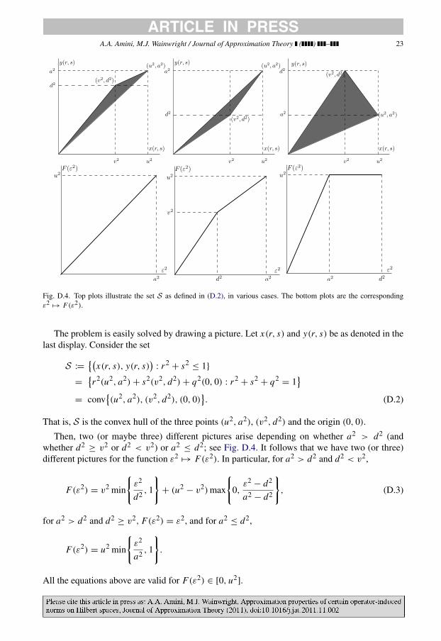
Fig. D.4. Top plots illustrate the set S as defined in (D.2), in various cases. The bottom plots are the correspondingε2

→ F(ε2).

The problem is easily solved by drawing a picture. Let x(r, s) and y(r, s) be as denoted in thelast display. Consider the set

S :=

x(r, s), y(r, s)

: r2+ s2

≤ 1}

=r2(u2, a2)+ s2(v2, d2)+ q2(0, 0) : r2

+ s2+ q2

= 1

= conv(u2, a2), (v2, d2), (0, 0)

. (D.2)

That is, S is the convex hull of the three points (u2, a2), (v2, d2) and the origin (0, 0).

Then, two (or maybe three) different pictures arise depending on whether a2 > d2 (andwhether d2

≥ v2 or d2 < v2) or a2≤ d2; see Fig. D.4. It follows that we have two (or three)

different pictures for the function ε2→ F(ε2). In particular, for a2 > d2 and d2 < v2,

F(ε2) = v2 min

ε2

d2 , 1

+ (u2

− v2)max

0,ε2

− d2

a2 − d2

, (D.3)

for a2 > d2 and d2≥ v2, F(ε2) = ε2, and for a2

≤ d2,

F(ε2) = u2 min

ε2

a2 , 1

.

All the equations above are valid for F(ε2) ∈ [0, u2].


Appendix E. Details of the Fourier truncation example

Here we establish the claim that the bound (19) holds with equality. Recall that for the(generalized) Fourier truncation operator Tψn

1, we have

RTψn1(ε) = sup

∞−

k=1

σkα2k :

∞−k=1

α2k ≤ 1,

n−k=1

σkα2k ≤ ε2

.

Let α = (tξ, sγ ), where t, s ∈ R, ξ = (ξ1, . . . , ξn) ∈ Rn, γ = (γ1, γ2, . . .) ∈ ℓ2 and‖ξ‖2 = 1 = ‖γ ‖2. Let u2

= u2(ξ) :=∑n

k=1 σkξ2k and v2

= v2(γ ) :=∑

k>n σkγ2k .

Let us fix ξ and γ for now and try to optimize over t and s. That is, we look at

G(ε2; ξ, γ ) := sup

t2u2

+ s2v2: t2

+ s2≤ 1, t2u2

≤ ε2.

This is an instance of the 2-by-2 problem (D.1), with a2= u2 and d2

= 0. Note that ourassumption that u2

≥ v2 holds in this case, for all ξ and γ , because {σk} is a nonincreasingsequence. Hence, we have, for ε2

≤ σ1,

G(ε2; ξ, γ ) = v2

+ (u2− v2)

ε2

u2 = v2(γ )+

1 −

v2(γ )

u2(ξ)

ε2.

Now we can maximize G(ε2; ξ, γ ) over ξ and then γ . Note that G is increasing in u2. Thus,

the maximum is achieved by selecting u2 to be sup‖ξ‖2=1 u2(ξ) = σ1. Thus,

supξ

G(ε2; ξ, γ ) =

1 −

ε2

σ1

v2(γ )+ ε2.

For ε2 < σ1, the above is increasing in v2. Hence the maximum is achieved by setting v2 to besup‖γ ‖2=1 v

2(γ ) = σn+1. Hence, for ε2≤ σ1

RTψn1(ε) := sup

ξ,γ

G(ε2; ξ, γ ) =

1 −

σn+1

σ1

ε2

+ σn+1. (E.1)

Appendix F. An quadratic inequality

In this appendix, we derive an inequality which will be used in the proof of Theorem 1.Consider a positive semidefinite matrix M (possibly infinite-dimensional) partitioned as

M =

A C

CT D

.

Assume that there exists ρ2∈ (0, 1) and κ2 > 0 such that

A CCT (1 − ρ2)D + κ2 I

≽ 0. (F.1)

Let (x, y) be a vector partitioned to match the block structure of M . Then we have the following.


Lemma 5. Under (F.1), for all x and y,

xT Ax + 2xT Cy + yT Dy ≥ ρ2xT Ax −κ2

1 − ρ2 ‖y‖22. (F.2)

Proof. By assumption (F.1), we have

1 − ρ2xT 1

1 − ρ2yT

A CCT (1 − ρ2)D + κ2 I

1 − ρ2x

11 − ρ2

y

≥ 0. � (F.3)

Writing (F.1) as a perturbation of the original matrix,A C

CT D

+

0 00 −ρ2 D + κ2 I

≽ 0, (F.4)

we observe that a sufficient condition for (F.1) to hold is ρ2 D ≼ κ2 I . That is, it is sufficient tohave

ρ2λmax(D) ≤ κ2. (F.5)

Rewriting (F.1) differently, as(1 − ρ2)A 0

0 (1 − ρ2)D

+

ρ2 A CCT κ2 I

≽ 0, (F.6)

we find another sufficient condition for (F.1), namely, ρ2 A − κ−2CCT≽ 0. In particular, it is

also sufficient to have

κ−2λmax(CCT ) ≤ ρ2λmin(A). (F.7)

References

[1] R. Adamczak, A tail inequality for suprema of unbounded empirical processes with applications to Markov chains,Electronic Journal of Probability 13 (2008) 1000–1034.

[2] R. Ahlswede, A. Winter, Strong converse for identification via quantum channels, IEEE Transactions onInformation Theory 48 (3) (2002) 569–579. doi:10.1109/18.985947.

[3] P.L. Bartlett, O. Bousquet, S. Mendelson, Local Rademacher complexities, Annals of Statistics 33 (4) (2005)1497–1537.

[4] R. DeVore, Approximation of functions, in: Proc. Symp. Applied Mathematics, vol. 36, 1986, pp. 1–20.[5] R.V. Gamkrelidze, D. Newton, V.M. Tikhomirov, Analysis: Convex Analysis and Approximation Theory,

Birkhauser, 1990.[6] D.J.H. Garling, Inequalities: A Journey into Linear Analysis, Cambridge Univ Pr., 2007.[7] V. Koltchinski, Local Rademacher complexities and oracle inequalities in risk minimization, Annals of Statistics

34 (6) (2006) 2593–2656.[8] M. Ledoux, The Concentration of Measure Phenomenon, in: Mathematical Surveys and Monographs, American

Mathematical Society, Providence, RI, 2001.[9] S. Mendelson, Geometric Parameters of Kernel Machines, in: Lecture Notes in Computer Science, vol. 2375, 2002,

pp. 29–43.[10] A. Pinkus, N -Widths in Approximation Theory, in: Ergebnisse der Mathematik und ihrer Grenzgebiete 3 Folge,

Springer, 1985.[11] A. Pinkus, N -widths and optimal recovery, in: Proc. Symp. Applied Mathematics, vol. 36, 1986, pp. 51–66.[12] G. Raskutti, M.J. Wainwright, B. Yu, Minimax-optimal rates for sparse additive models over kernel classes via

convex programming, Tech. Rep., Department of Statistics, UC Berkeley, August 2010.http://arxiv.org/abs/1008.3654.

http://dx.doi.org/doi:10.1109/18.985947

http://arxiv.org/1008.3654


[13] F. Riesz, B. Sz.-Nagy, Functional Analysis, Dover Publications, 1990.[14] M. Rudelson, Random vectors in the isotropic position, Journal of Functional Analysis 164 (1) (1999) 60–72.

doi:10.1006/jfan.1998.3384.[15] J.A. Tropp, User-friendly tail bounds for sums of random matrices.

URL: arxiv:1004.4389]http://arxiv.org/abs/1004.4389.[16] S.A. van de Geer, Empirical Processes in M-Estimation, Cambridge University Press, 2000.[17] A.W. van der Vaart, J. Wellner, Weak Convergence and Empirical Processes, Springer-Verlag, New York, NY, 1996.[18] R. Vershynin, Introduction to the non-asymptotic analysis of random matrices.

URL: http://www-personal.umich.edu/˜romanv/papers/non-asymptotic-rmt-plain.pdf.[19] A. Wigderson, D. Xiao, Derandomizing the Ahlswede–Winter matrix-valued Chernoff bound using pessimistic

estimators, and applications, Theory of Computing 4 (1) (2008) 53–76. doi:10.4086/toc.2008.v004a003.

http://dx.doi.org/doi:10.1006/jfan.1998.3384

http://www-personal.umich.edu/~romanv/papers/non-asymptotic-rmt-plain.pdf

http://dx.doi.org/doi:10.4086/toc.2008.v004a003

Documents

Approximation properties of certain operator-induced norms ...wainwrig/Papers/AmiWai11.pdf · 4 A.A. Amini, M.J. Wainwright / Journal of Approximation Theory ( ) – Hilbert sequence