Approximation Techniques Approximation Techniques for Data Management for Data Management

SystemsSystems

““We are drowning in data but We are drowning in data but starved for knowledge”starved for knowledge”

John NaisbittJohn Naisbitt

CS 186Fall 2005

2

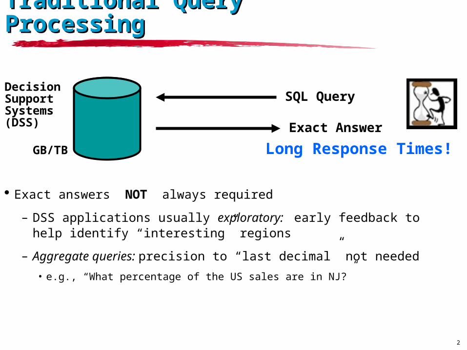
Traditional Query Traditional Query ProcessingProcessing

Exact answers NOT always required

– DSS applications usually exploratory: early feedback to help identify “interesting” regions

– Aggregate queries: precision to “last decimal” not needed

• e.g., “What percentage of the US sales are in NJ?”

SQL Query

Exact Answer

DecisionSupport Systems(DSS)

Long Response Times!

GB/TB

3

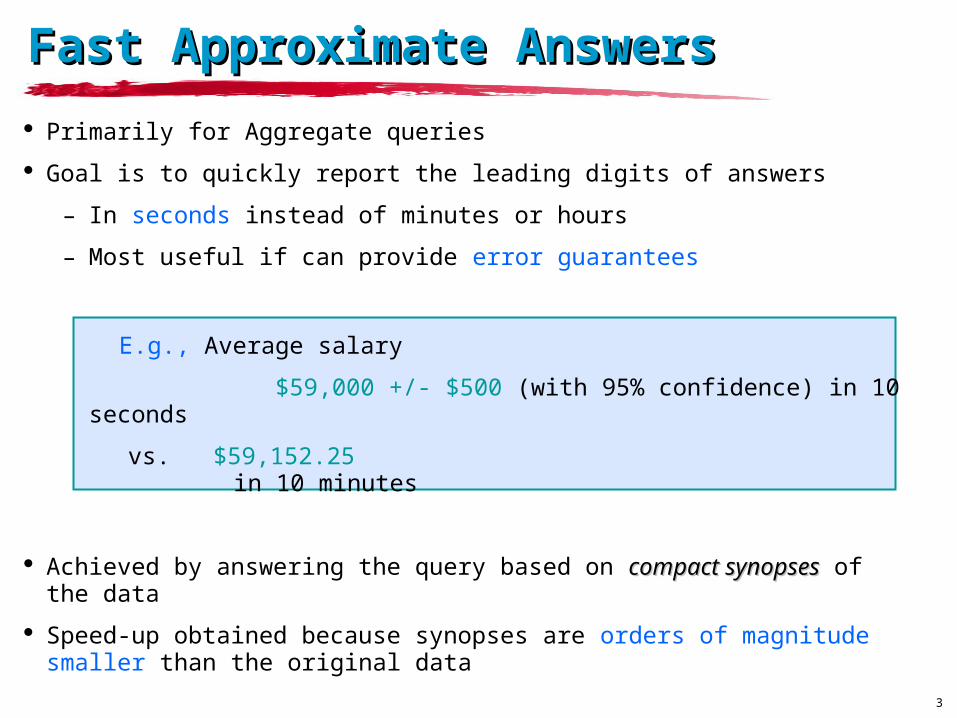
Primarily for Aggregate queries

Goal is to quickly report the leading digits of answers

– In seconds instead of minutes or hours

– Most useful if can provide error guarantees

E.g., Average salary

$59,000 +/- $500 (with 95% confidence) in 10 seconds

vs. $59,152.25 in 10 minutes

Achieved by answering the query based on compact synopsescompact synopses of the data

Speed-up obtained because synopses are orders of magnitude smaller than the original data

Fast Approximate AnswersFast Approximate Answers

4

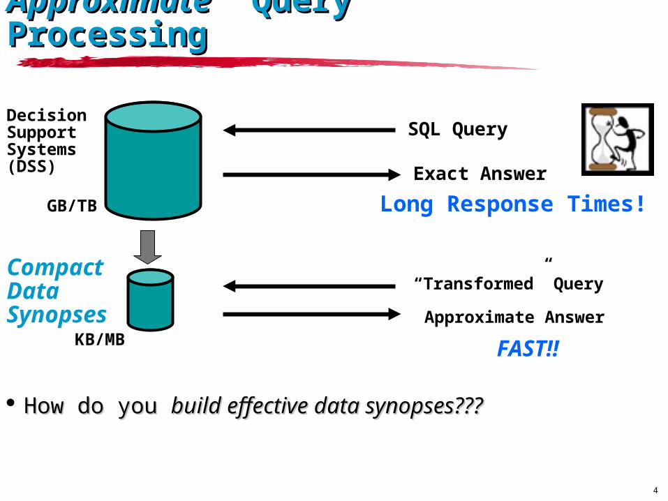
ApproximateApproximate Query Query ProcessingProcessing

How do you How do you build effective data synopses???build effective data synopses???

SQL Query

Exact Answer

DecisionSupport Systems(DSS)

Long Response Times!

GB/TB

Compact Data Synopses

“Transformed” Query

KB/MBApproximate Answer

FAST!!

5

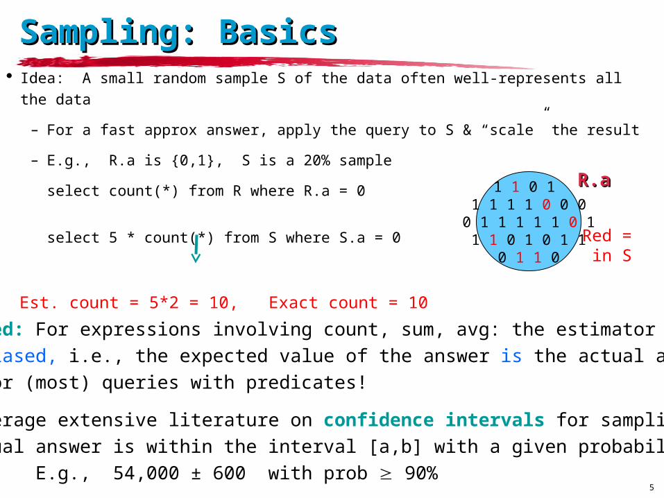
Sampling: BasicsSampling: Basics Idea: A small random sample S of the data often well-represents all the data

– For a fast approx answer, apply the query to S & “scale” the result

– E.g., R.a is {0,1}, S is a 20% sample

select count(*) from R where R.a = 0

select 5 * count(*) from S where S.a = 0

1 1 0 1 1 1 1 1 0 0 0

0 1 1 1 1 1 0 11 1 0 1 0 1 1

0 1 1 0

Red = in S

R.aR.a

Est. count = 5*2 = 10, Exact count = 10

Unbiased: For expressions involving count, sum, avg: the estimatoris unbiased, i.e., the expected value of the answer is the actual answer,even for (most) queries with predicates!

• Leverage extensive literature on confidence intervals for samplingActual answer is within the interval [a,b] with a given probability

E.g., 54,000 ± 600 with prob 90%

6

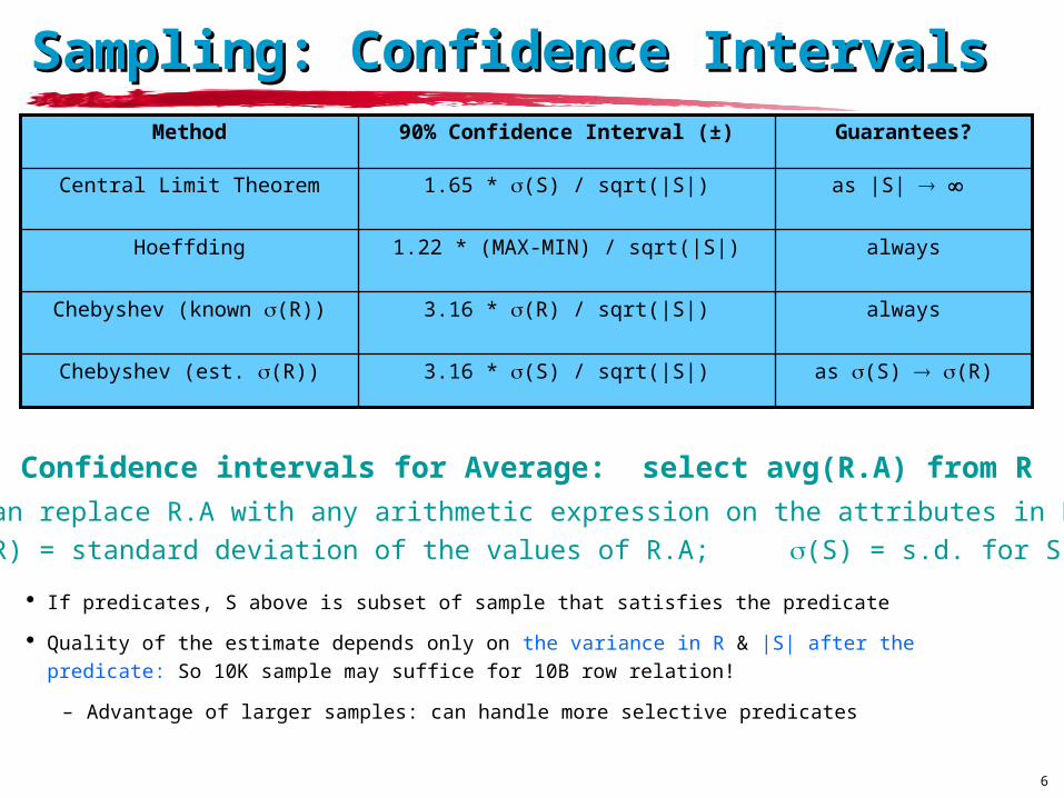
Sampling: Confidence IntervalsSampling: Confidence Intervals

If predicates, S above is subset of sample that satisfies the predicate

Quality of the estimate depends only on the variance in R & |S| after the predicate: So 10K sample may suffice for 10B row relation!

– Advantage of larger samples: can handle more selective predicates

Guarantees?90% Confidence Interval (±)Method

as (S) (R)3.16 * (S) / sqrt(|S|)Chebyshev (est. (R))

always3.16 * (R) / sqrt(|S|)Chebyshev (known (R))

always1.22 * (MAX-MIN) / sqrt(|S|)Hoeffding

as |S| 1.65 * (S) / sqrt(|S|)Central Limit Theorem

Confidence intervals for Average: select avg(R.A) from R

(Can replace R.A with any arithmetic expression on the attributes in R)(R) = standard deviation of the values of R.A; (S) = s.d. for S.A

7

Sampling from DatabasesSampling from Databases Sampling disk-resident data is slow

– Row-level sampling has high I/O cost:

• must bring in entire disk block to get the row

– Block-level sampling: rows may be highly correlated

– Random access pattern, possibly via an index

– Need to account for the variable number of rows in a page, children in an index node, etc.

Alternatives

– Random physical clustering: destroys “natural” clustering

– Precomputed samples: must incrementally maintain (at specified size)

• Fast to use: packed in disk blocks, can sequentially scan, can store as relation and leverage full DBMS query support, can store in main memory

8

One-Pass Uniform SamplingOne-Pass Uniform Sampling

Best choice for incremental maintenance

– Low overheads, no random data access

Reservoir Sampling [Vit85]: Maintains a sample S of a fixed-size MMaintains a sample S of a fixed-size M

– Add each new item to S with probability M/N, where N is the current number of data items

– If add an item, evict a random item from S

– Instead of flipping a coin for each item, determine the number of items to skip before the next to be added to S

9

HistogramsHistograms

Partition attribute value(s) domain into a set of buckets

Issues:

– How to partition

– What to store for each bucket

– How to estimate an answer using the histogram

Long history of use for selectivity estimation within a query optimizer

Recently explored as a tool for fast approximate query processing

10

1-D Histograms1-D Histograms

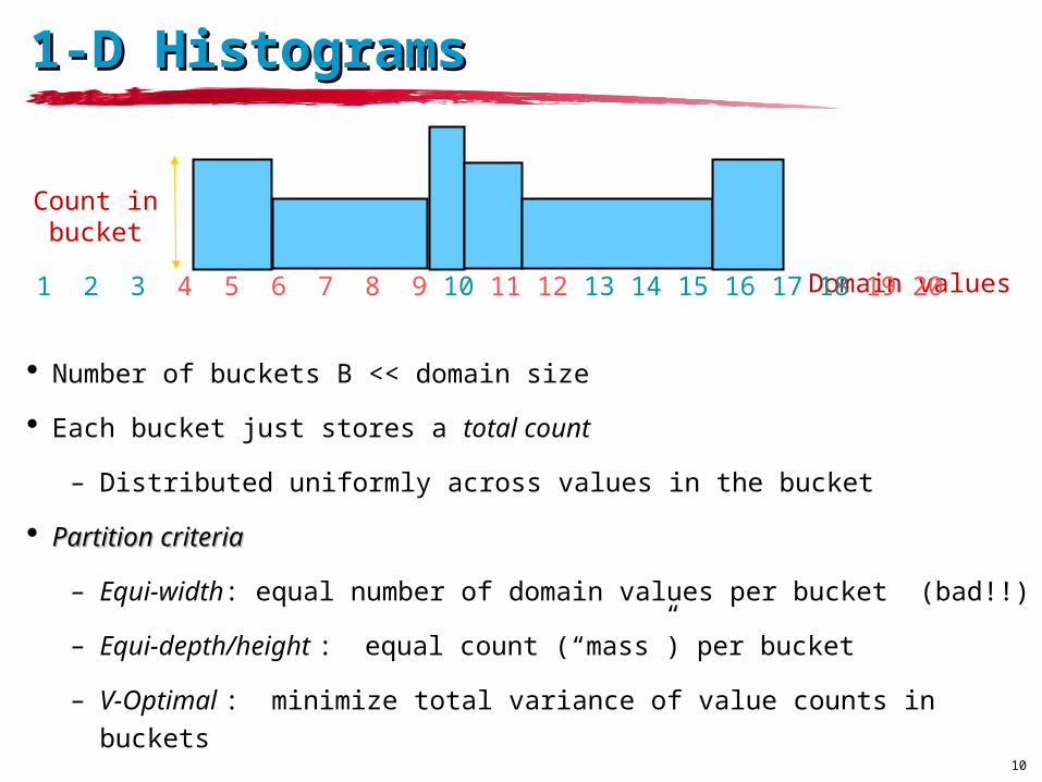
Number of buckets B << domain size

Each bucket just stores a total count

– Distributed uniformly across values in the bucket

Partition criteriaPartition criteria

– Equi-width: equal number of domain values per bucket (bad!!)

– Equi-depth/height : equal count (“mass”) per bucket

– V-Optimal : minimize total variance of value counts in buckets

Count inbucket

Domain values1 2 3 4 5 6 7 8 9 10 11 12 13 14 15 16 17 18 19 20

11

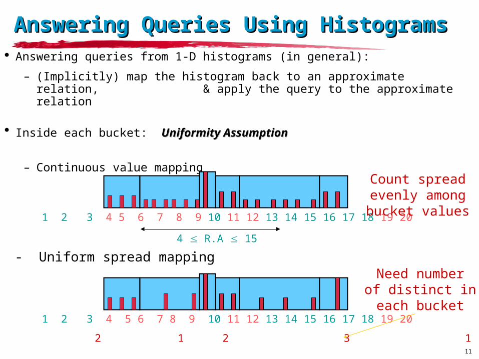
Answering Queries Using HistogramsAnswering Queries Using Histograms Answering queries from 1-D histograms (in general):

– (Implicitly) map the histogram back to an approximate relation, & apply the query to the approximate relation

Inside each bucket: Uniformity AssumptionUniformity Assumption

– Continuous value mapping

1 2 3 4 5 6 7 8 9 10 11 12 13 14 15 16 17 18 19 20

1 2 3 4 5 6 7 8 9 10 11 12 13 14 15 16 17 18 19 20

Need numberof distinct ineach bucket

3 2 1 2 3 1

Count spreadevenly amongbucket values

- Uniform spread mapping4 R.A 15

12

Haar Wavelet SynopsesHaar Wavelet Synopses

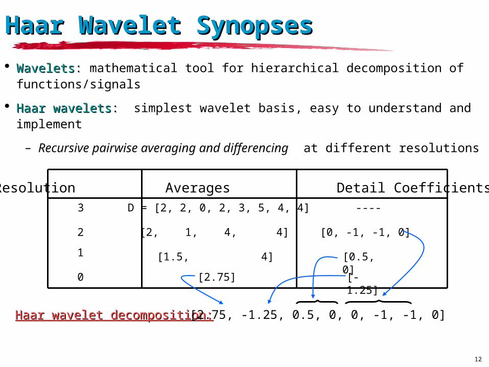
WaveletsWavelets:: mathematical tool for hierarchical decomposition of functions/signals

Haar waveletsHaar wavelets:: simplest wavelet basis, easy to understand and implement

– Recursive pairwise averaging and differencing at different resolutions

Resolution Averages Detail CoefficientsD = [2, 2, 0, 2, 3, 5, 4, 4]

[2, 1, 4, 4] [0, -1, -1, 0]

[1.5, 4] [0.5, 0]

[2.75] [-1.25]

----3

2

1

0

Haar wavelet decomposition:Haar wavelet decomposition: [2.75, -1.25, 0.5, 0, 0, -1, -1, 0]

13

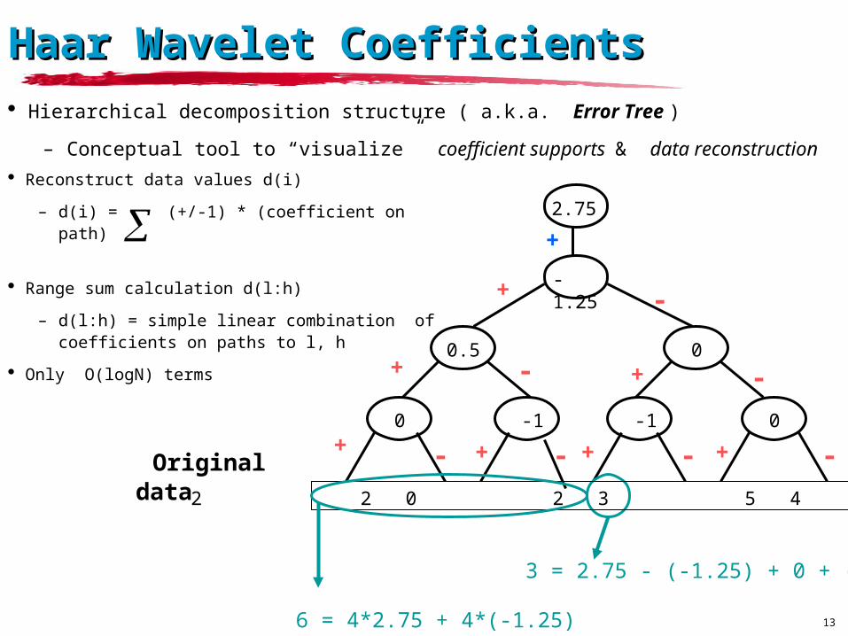
Haar Wavelet Coefficients Haar Wavelet Coefficients Hierarchical decomposition structure ( a.k.a. Error Tree )

– Conceptual tool to “visualize” coefficient supports & data reconstruction Reconstruct data values d(i)

– d(i) = (+/-1) * (coefficient on path)

Range sum calculation d(l:h)

– d(l:h) = simple linear combination of coefficients on paths to l, h

Only O(logN) terms

2 2 0 2 3 5 4 4

-1.25

2.75

0.5 0

0 -1 0 -1

+

-+

+

+ + +

+

+

- -

- - - - Original data

3 = 2.75 - (-1.25) + 0 + (-1)

6 = 4*2.75 + 4*(-1.25)

14

Wavelet Data Synopses Wavelet Data Synopses

Compute Haar wavelet decomposition of D

Coefficient thresholding : only B<<|D| coefficients can be kept

– B is determined by the available synopsis space

Approximate query engine can do all its processing over such compact coefficient synopses (joins, aggregates, selections, etc.)

Conventional thresholding: Take B largest coefficients in absolute normalized value

– Normalized Haar basis: divide coefficients at resolution j by

– All other coefficients are ignored (assumed to be zero)

– Provably optimal in terms of the overall Sum-Squared (L2) Error

j2

15

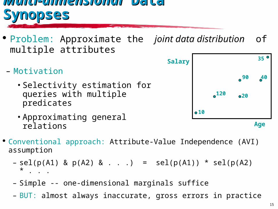
Multi-dimensionalMulti-dimensional Data Data Synopses Synopses

Problem: Approximate the joint data distribution of multiple attributes

– Motivation

•Selectivity estimation for queries with multiple predicates

•Approximating general relations 10

20

40

35

90

120

Age

Salary

Conventional approach: Attribute-Value Independence (AVI) assumption

– sel(p(A1) & p(A2) & . . .) = sel(p(A1)) * sel(p(A2) * . . .

– Simple -- one-dimensional marginals suffice

– BUT: almost always inaccurate, gross errors in practice

16

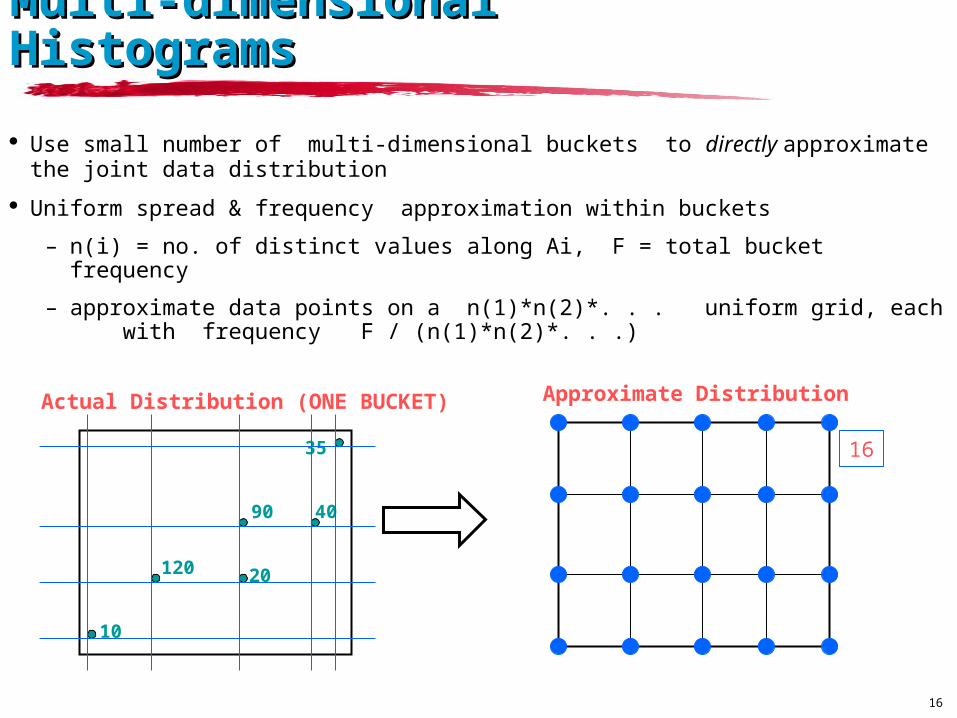
Multi-dimensional Multi-dimensional Histograms Histograms

Use small number of multi-dimensional buckets to directly approximate the joint data distribution

Uniform spread & frequency approximation within buckets

– n(i) = no. of distinct values along Ai, F = total bucket frequency

– approximate data points on a n(1)*n(2)*. . . uniform grid, each with frequency F / (n(1)*n(2)*. . .)

10

20

40

35

90

120

Actual Distribution (ONE BUCKET)

16

Approximate Distribution

17

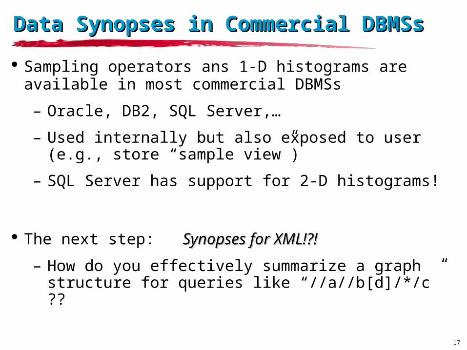
Data Synopses in Commercial DBMSsData Synopses in Commercial DBMSs

Sampling operators ans 1-D histograms are available in most commercial DBMSs

– Oracle, DB2, SQL Server,…

– Used internally but also exposed to user (e.g., store “sample view”)

– SQL Server has support for 2-D histograms!

The next step: Synopses for XML!?!Synopses for XML!?!

– How do you effectively summarize a graph structure for queries like “//a//b[d]/*/c” ??

18

Data-Stream ManagementData-Stream Management Traditional DBMS – data stored in finite, persistent

data setsdata sets

Data Streams – distributed, continuous, unbounded, rapid, time varying, noisy, . . .

Data-Stream Management – variety of modern applications

– Network monitoring and traffic engineering– Telecom call-detail records– Network security – Financial applications– Sensor networks– Web logs and clickstreams

19

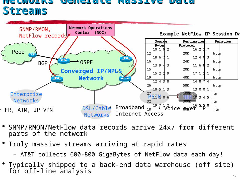
Networks Generate Massive Data Networks Generate Massive Data Streams Streams

• Broadband Internet Access

Converged IP/MPLSNetwork

PSTN

DSL/CableNetworks

EnterpriseNetworks

• Voice over IP• FR, ATM, IP VPN

Network OperationsCenter (NOC)

SNMP/RMON,NetFlow records

BGP OSPF

Peer

SNMP/RMON/NetFlow data records arrive 24x7 from different parts of the network

Truly massive streams arriving at rapid rates

– AT&T collects 600-800 GigaBytes of NetFlow data each day!

Typically shipped to a back-end data warehouse (off site) for off-line analysis

Source Destination Duration Bytes Protocol 10.1.0.2 16.2.3.7 12 20K http 18.6.7.1 12.4.0.3 16 24K http 13.9.4.3 11.6.8.2 15 20K http 15.2.2.9 17.1.2.1 19 40K http 12.4.3.8 14.8.7.4 26 58K http 10.5.1.3 13.0.0.1 27 100K ftp 11.1.0.6 10.3.4.5 32 300K ftp 19.7.1.2 16.5.5.8 18 80K ftp

Example NetFlow IP Session Data

20

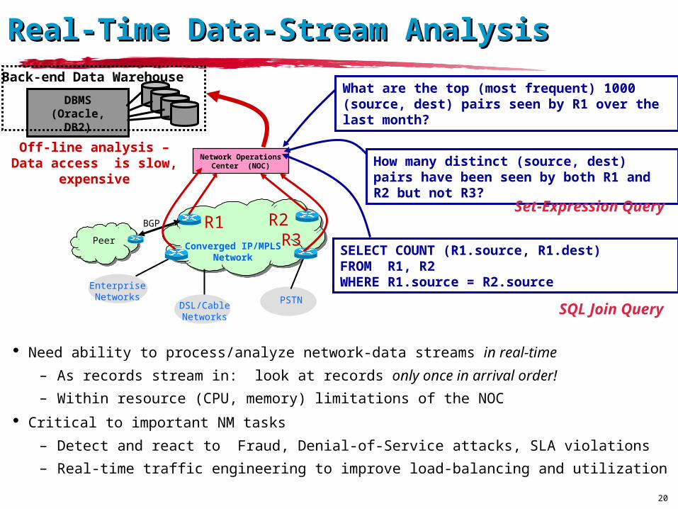
Real-Time Data-Stream Analysis Real-Time Data-Stream Analysis

Need ability to process/analyze network-data streams in real-time

– As records stream in: look at records only once in arrival order!

– Within resource (CPU, memory) limitations of the NOC

Critical to important NM tasks

– Detect and react to Fraud, Denial-of-Service attacks, SLA violations

– Real-time traffic engineering to improve load-balancing and utilization

DBMS(Oracle, DB2)

Back-end Data Warehouse

Off-line analysis – Data access is slow,

expensive

Converged IP/MPLSNetwork

PSTNDSL/CableNetworks

EnterpriseNetworks

Network OperationsCenter (NOC)

BGP

Peer

R1 R2R3

What are the top (most frequent) 1000 (source, dest) pairs seen by R1 over the last month?

SELECT COUNT (R1.source, R1.dest)FROM R1, R2WHERE R1.source = R2.source

SQL Join Query

How many distinct (source, dest) pairs have been seen by both R1 and R2 but not R3?

Set-Expression Query

21

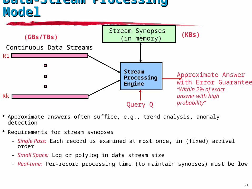
DataData--StreamStream ProcessingProcessing ModelModel

Approximate answers often suffice, e.g., trend analysis, anomaly detection

Requirements for stream synopses

– Single Pass: Each record is examined at most once, in (fixed) arrival order

– Small Space: Log or polylog in data stream size

– Real-time: Per-record processing time (to maintain synopses) must be low

Stream ProcessingEngine

Approximate Answerwith Error Guarantees“Within 2% of exactanswer with highprobability”

Stream Synopses (in memory)

Continuous Data Streams

Query Q

R1

Rk

(GBs/TBs) (KBs)

22

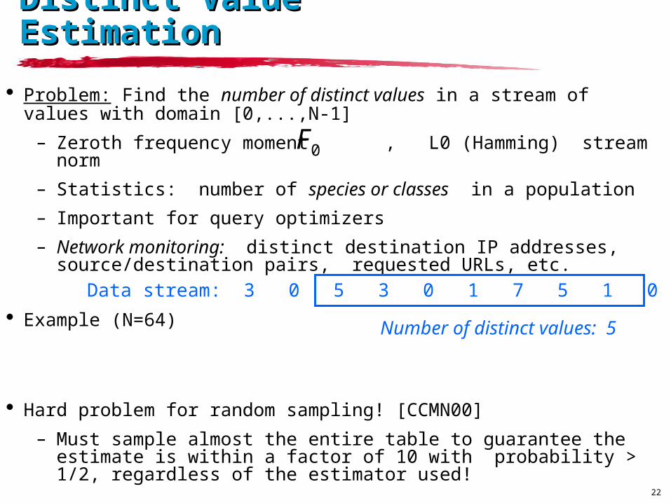
Distinct Value EstimationDistinct Value Estimation

Problem: Find the number of distinct values in a stream of values with domain [0,...,N-1]

– Zeroth frequency moment , L0 (Hamming) stream norm

– Statistics: number of species or classes in a population

– Important for query optimizers

– Network monitoring: distinct destination IP addresses, source/destination pairs, requested URLs, etc.

Example (N=64)

Hard problem for random sampling! [CCMN00]

– Must sample almost the entire table to guarantee the estimate is within a factor of 10 with probability > 1/2, regardless of the estimator used!

Data stream: 3 0 5 3 0 1 7 5 1 0 3 7

Number of distinct values: 5

0F

23

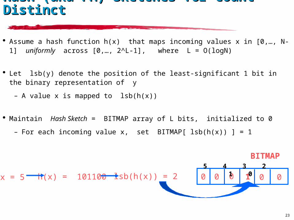
Assume a hash function h(x) that maps incoming values x in [0,…, N-1] uniformly across [0,…, 2^L-1], where L = O(logN)

Let lsb(y) denote the position of the least-significant 1 bit in the binary representation of y

– A value x is mapped to lsb(h(x))

Maintain Hash Sketch = BITMAP array of L bits, initialized to 0

– For each incoming value x, set BITMAP[ lsb(h(x)) ] = 1

Hash (aka FM) Sketches for Count Hash (aka FM) Sketches for Count DistinctDistinct

x = 5 h(x) = 101100 lsb(h(x)) = 2 0 0 0 001

BITMAP5 4 3 2 1 0

24

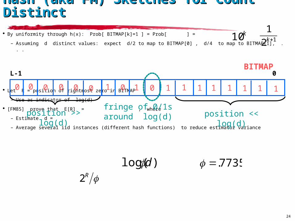
Hash (aka FM) Sketches for Count Hash (aka FM) Sketches for Count Distinct Distinct By uniformity through h(x): Prob[ BITMAP[k]=1 ] = Prob[ ] =

– Assuming d distinct values: expect d/2 to map to BITMAP[0] , d/4 to map to BITMAP[1], . . .

Let R = position of rightmost zero in BITMAP

– Use as indicator of log(d)

[FM85] prove that E[R] = , where

– Estimate d =

– Average several iid instances (different hash functions) to reduce estimator variance

fringe of 0/1s around log(d)

0 0 0 00 1

BITMAP

0 00 111 1 11111

position << log(d)

position >> log(d)

)log( d 7735.R2

k10 12

1k

0L-1

25

A Little Streaming Puzzle…A Little Streaming Puzzle…

Input: A stream of N numbers/elements

Output: The stream majority element (if one exists)

– e is a majority element if frequency(e) > N/2

Q: How do you do this in small space??

– Hint: Use just two memory locations

– Hint++: Look at this as a “knockout tournament”

Feeling adventurous?

– How do you do the same majority query over a stream of insertions and deletions?

– Input: Stream of <e, +> = insert e , <e, -> = delete e

– Hint: Use a little more memory…

26

In Summary: Not your parents’ In Summary: Not your parents’ DBMS!DBMS!

Database/data-management research goes far beyond the basics!

Extends from distributed systems to theory to approximation algorithms to probability/statistics to …

– Applications: data mining, sensornets, p2p, …

– Just pick up a copy of recent SIGMOD/VLDB proceedings

More and more relevant in dealing with the “data tsunami”

– Data is everywhere! And, it’s constantly growing in volume!

Exciting, relevant research!

27

More details…More details…

http://www2.berkeley.intel-research.net/~minos/tutorials.html

•Tutorial slides on approximate query processing and data streams