Embed Size (px)
Citation preview
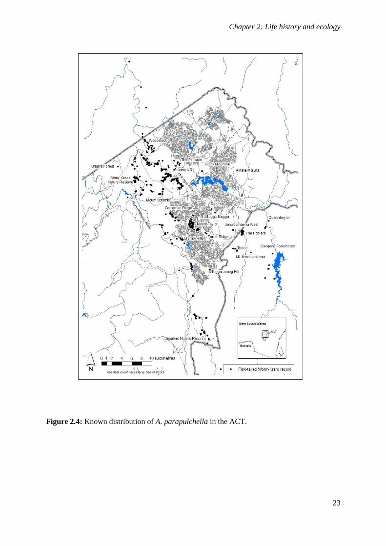
Environmental factors affecting the occurrence and
abundance of the Pink-tailed Worm-lizard
(Aprasia parapulchella) in the
Australian Capital Territory
David Thye Yau Wong
BA (University of Sydney)
BSc (Australian National University)
Institute for Applied Ecology
Faculty of Applied Science
University of Canberra
Australia
A thesis submitted for the degree of Doctor of Philosophy at the
University of Canberra
May 2013
iii
v
Abstract
vii
Abstract
The effect of human-induced land use changes on biodiversity and ecosystem functioning is
something that we will increasingly need to grapple with. The loss and decline of the habitat
of species as a result of agricultural practices is one of the most pervasive threats to
biodiversity and current conservation measures are not successfully offsetting the effects of
this threat.
The Pink-tailed Worm-lizard (Aprasia parapulchella) is a disturbance sensitive
species of legless lizard which is listed as threatened at national and state levels in Australia.
The loss and decline of its habitat, as a result of agricultural practices, are thought to be the
major causes of its decline across its distributional range. However, the relationship between
the occurrence of this lizard and agricultural disturbance has not been examined in detail and
previous researchers have identified this gap in the knowledge about this species. Currently,
there is no synthesis of existing knowledge about A. parapulchella and the information is not
contained in the published scientific literature. Such a synthesis, combined with a more
detailed investigation of the environmental correlates of occurrence and predicted distribution
of the species, is likely to aid conservation efforts directed towards the species.
I aimed to address these gaps in the knowledge of the species at both the patch and
landscape/regional scales. In this thesis I provide a synthesis of the existing knowledge on the
life-history and ecology of A. parapulchella. In addition, I investigate the factors driving
occurrence and abundance of A. parapulchella in the ACT at the regional and patch scale.
Abstract
viii
Species distribution models are increasingly common tools being used for predicting
and explaining the distribution of species in space. These models are often used over a broad
spatial scale. I used MaxEnt to examine the relationship between environmental factors and
the occurrence of A. parapulchella at the regional scale using a fine grained analysis (30m
resolution). I also applied the novel use of a remotely-sensed classification discriminating
between C3 and C4 grasses within the model as a way of incorporating agricultural
modification as a variable. The results confirmed previously described relationships and add
to the existing knowledge. Soil type and geology made the highest contributions to the model
(29.4% and 20.3% respectively) followed by slope (15.5%), average minimum temperature in
October (13.2%), average rainfall in October (12.1%) and agricultural modification (9.5%).
New associations between likelihood of occurrence of A. parapulchella and climatic variables
were described. In addition an association between A. parapulchella and a Devonian-age
geological unit was identified for the first time in the Australian Capital Territory.
As I found that agricultural modification contributed to a species distribution model
for the occurrence of A. parapulchella in the Australian Capital Territory, the question of the
importance of this variable arose. Comparing models with and without agricultural
modification may also be a useful method to quantify habitat loss and degradation. I
compared models with and without the agricultural modification variable in order to assess
the extent to which incorporating agricultural modification improved the model. Including
agricultural modification led to a lower likelihood of predicting false positives (t = 2.32; p =
0.021), whilst the likelihood of correctly predicting presence was not significantly different
between models with and without agricultural modification. The model with agricultural
modification predicted more native grassy vegetation, whilst the model without the variable
predicted more exotic/degraded native grassy vegetation. The results of the modelling suggest
that at least approximately 40% of optimal habitat has declined in condition or been lost in the
Abstract
ix
evaluation area used in the study and at least approximately one-quarter of optimal habitat has
been lost or degraded in the Australian Capital Territory.
In order to investigate the factors influencing occurrence and abundance of
A. parapulchella at the patch scale, the abundance of A. parapulchella were recorded at sites
of varying levels of disturbance. Vegetation indicators of disturbance were derived and a
range of habitat attributes measured. The data were analysed using boosted regression trees.
Vegetation indices associated with disturbance were the best predictors in the model. The
percentage cover of large tussock grasses was identified as particularly influential in the
model. Other habitat variables made minor contributions to the model.
Taken together, the results suggest that loss and degradation of the ground layer
habitat of A. parapulchella, as a result of agricultural modification, has historically been the
major driver of decline of the species across its range. Whilst forestry and urbanisation remain
significant threats that need to be addressed simultaneously, their direct impact is often more
immediately obvious compared to those associated with agricultural modification. The
findings of my research suggest that, on private land, management that maintains rocky
habitat with a substantial cover of grasses from the large tussock functional group (as well as
suitable native grassy connections between rocky areas) will provide the best chance for
maintaining viable populations of A. parapulchella
Acknowledgements
xiii
Acknowledgements
Firstly, I wish to acknowledge the Ngunnawal people, both past and present, the
traditional owners and custodians of the land on which I live and conducted my research.
These past few years have been a great experience for me and I am extremely grateful
to all the people who have helped me in various ways throughout my PhD journey. Without
you all I couldn’t have done it. In the timeless words of Jeff Fenech: “I love youse all”! I hope
that I can remember everyone, but if there is anyone who I have inadvertently missed, I
sincerely apologise.
I have been blessed with an excellent supervisory panel. Each of my supervisors has
helped me immensely. Thanks to their expert guidance, I have learnt so much about
questioning, writing and how to operate in the world of science and academia. I am lucky to
be able to consider them as mentors as well as friends.
To my primary supervisor, Will Osborne, thank you so much for your continued
support and guidance throughout the duration of the project. I feel very lucky to have received
tutelage from a great herpo, naturalist and ecologist. Your detailed knowledge of the species
and the land were invaluable and your generosity and guidance played a large role in ensuring
my completion of the thesis.
To my associate supervisors, Stephen Sarre and Bernd Gruber; you have both played
crucial roles in helping me to get to this point. Thank you, Stephen, for your incisive
comments and insights. They helped me to keep the big picture in mind whilst also focussing
on the details. I am also very grateful for your ongoing support and timely intervention at a
critical point in the project. Bernd, I feel very lucky that you joined the supervisory panel.
Your expertise in statistics and modelling were invaluable. Your committed support and
generosity with your time and expertise as a supervisor, and as HDR co-ordinator, was greatly
appreciated (by me and all the HDR students).
The project would not have been possible without the funding provided by ACT Parks
Conservation and Lands. I also received valuable support, background information and data
from various people in ACT Government including (in no particular order): Marjo Rauhala,
Darren Roso, Sharon Lane, Margaret Kitchin, Murray Evans, Greg Baines, Don Fletcher,

Acknowledgements
xiv
Felicity Grant, Graeme Hirth, Kevin Frawley, Luke Johnston, Lesley Ishiyama and Danny
Orwin, Daniel Goodwin, Nadia Kuzmanoski, Maree Gilbert, Lara Woolcombe, Kristy Gould,
Peter Galvin and Veronica Collins.
A range of other people generously gave their time to support the project in various
ways including helping with project design and statistical analysis, providing data,
collaborating on papers and discussing ideas. I therefore thank: Sandie Jones, Rainer
Rehwinkel and David Hunter of NSW Office of Environment and Heritage; Mike Austin, Sue
McIntyre, Jacqui Stol and Josh Dorrough of CSIRO; Geoff Brown and Arn Tolsma of the
Arthur Rylah Institute; John Wainer (Department of Primary Resources, Victoria); Mark
Dunford (Geoscience Australia); Shawn Laffan (University of NSW); Ingrid Stirnemann,
Annabel Smith, Phil Gibbons, Malcolm Gill, Damian Michael and Geoffrey Kay of the
Australian National University; Dennis Black (La Trobe University); Theresa Knopp
(Institute for Applied Ecology, University of Canberra); Peter Robertson (Wildlife Profiles);
Tom O’Sullivan (Bluegum Ecological Consulting); Aaron Organ (Ecology and Heritage
Partners) and; Steve Sass (EnviroKey).
I could not have completed my fieldwork without the help of many people who helped
me in the field. Turning thousands of rocks is not everyone’s idea of fun, but you all helped to
make it a pleasure. For all your help, I sincerely thank: Dana Weinhold, Sylvio Teubert, Anett
Richter, Anna See, Arne Bishop, Mark Bradley, Berlinda Bowler, Liam Seed, Cameron Hall,
Melanie McGregor, Matthew Young, Amy O’Brien, Lesley Ishiyama, Annabel Smith, Ingrid
Stirnemann and students from CIT and the University of Canberra Conservation Biology class
(2009; 2010). Mork Ratanakosol, in particular, devoted many days to helping me in the field.
Special thanks also go to Sam Walker, who was an enormous help with data entry. A number
of landholders generously allowed me access to their land to undertake survey or invited me
to survey on their land. Therefore, I sincerely thank Michael Retallack, Gordon Hughes,
Maurice Tully, John Gale and Steven Guth.
Many staff at the Institute for Applied Ecology helped to ensure that the project ran
smoothly through their technical or administrative support. Therefore, I wish to thank (in no
particular order): Peter Ogilvie, Antony Senior, Mark Jillard, Richard Carne, Vicki Smyth,
Barbara Harris, Jo Shevchenko, Helen Thomas, Kerrie Aust, Jayne Lawrence and Joanne
Sutherland. There are too many people from the institute to name individually, but I am
thankful to have had the chance to get to know many of you.

Acknowledgements
xv
Throughout my time at the University of Canberra I have made many great friendships
and enjoyed chats in the corridor or tea room with many people. In particular, the research
student group and early career researchers have formed wonderful support network. Thank
you to in particular to: Kate Hodges, Carla Eisemberg, Bruno Ferronato, Maria Boyle,
Veronika Vysna, Larissa Schneider Guilhon, Anett Richter, Wendy Dimond, Michael Jensen,
Anna MacDonnald, Niccy Aitken, Matthew Young, Stewart Pittard, Sam Walker, Tim
McGrath and Theresa Knopp. It has been a real pleasure.
I would also like to thank sincerely, Joelle Vandermensbrugghe and Bernd Gruber for
their support at various times during my candidature. Your generous support of the welfare of
HDR students is very much appreciated.
Second last, but definitely not least, thank you to all the Pink-tailed Worm-lizards who
were involved in this study. I wish you and your kind, many more days on this earth.
And finally, thank you to all my close friends and family who supported me for the
duration of the project. Thank you for your support, tolerance and encouragement. To Sonya
Duus, Nicole Maron, Ingrid Stirnemann, David Leigh and Annabel Smith, Percy Wong and
Elisabeth Wong, thank you for your generous editorial advice. To Mum, Dad, Justin and
Michael, thank you for being there during this time and throughout my life. And, to my lovely
wife Sonoko Wakikaido, thank you for all your belief, tolerance and support.
All research undertaken for this thesis was approved by the University of Canberra Committee for Ethics in Animal
Experimentation (project authorisation code CEAE08-17). Field work was carried out under licence, in accordance with the
Nature Conservation Act 1980 (Licence no. LT2008311).
Table of Contents
xvii
Table of Contents
Abstract .................................................................................................................................... vii
Form B ....................................................................................................................................... xi
Certificate of Authorship of Thesis .......................................... Error! Bookmark not defined.
Acknowledgements ................................................................................................................. xiii
Table of Contents ................................................................................................................... xvii
List of Figures ....................................................................................................................... xxiii
List of Tables .......................................................................................................................... xxv
1. Introduction ............................................................................................................ 1
Background ....................................................................................................... 1
Species Distribution Models ............................................................................. 2
The importance of niche ......................................................................................... 3
Model types and usage ........................................................................................... 4
Presence/absence or presence-only? ...................................................................... 7
Are the times a changing? ...................................................................................... 7
The case study of a threatened species in a changing world ............................. 8
Aims and structure of this thesis ..................................................................... 12
2. The life history and ecology of the Pink-tailed Worm-lizard (Aprasia
parapulchella) Kluge – a review .............................................................................................. 15
Abstract ........................................................................................................... 15
Introduction ..................................................................................................... 16
Taxonomy and morphology ............................................................................ 17
Biology and ecology ........................................................................................ 21
Distribution ...................................................................................................... 21
Habitat ............................................................................................................. 27
Table of Contents
xviii
Geology ................................................................................................................ 27
Soils ...................................................................................................................... 28
Aspect and slope ................................................................................................... 28
Vegetation ............................................................................................................ 29
Rocks and home sites ........................................................................................... 37
Population attributes ........................................................................................ 41
Reproduction ................................................................................................... 45
Activity patterns and movement ..................................................................... 46
Thermoregulation ............................................................................................ 48
Social behaviour .............................................................................................. 48
Relationship with ants ..................................................................................... 49
Diet .................................................................................................................. 50
Tail loss and predation .................................................................................... 51
Research directions ......................................................................................... 52
Conclusion ....................................................................................................... 52
Acknowledgements ......................................................................................... 53
3. Clarifying environmental correlates of occurrence for Aprasia parapulchella
using MaxEnt ........................................................................................................................... 55
Abstract ........................................................................................................... 55
Introduction ..................................................................................................... 56
Methods ........................................................................................................... 58
Study Area ............................................................................................................ 58
Selection of modelling package ........................................................................... 60
Data layer selection .............................................................................................. 60
Model running and optimisation .......................................................................... 62
Table of Contents
xix
Assessment of the model ...................................................................................... 63
Results ............................................................................................................. 63
Visual representation of the model ....................................................................... 65
Contribution of variables ...................................................................................... 67
Discussion ....................................................................................................... 75
Model performance .............................................................................................. 75
Visual representation of the model ....................................................................... 75
Contribution of variables ...................................................................................... 75
Habitat correlates .................................................................................................. 77
Interpretation of response ..................................................................................... 82
Conclusion ............................................................................................................ 83
Acknowledgements ......................................................................................... 84
4. Species distribution modelling for a disturbance-sensitive lizard: agricultural
modification matters ................................................................................................................. 85
Abstract ........................................................................................................... 85
Introduction ..................................................................................................... 87
Methods ........................................................................................................... 92
Study Area ............................................................................................................ 92
Selection of modelling package ........................................................................... 94
Data layer selection .............................................................................................. 94
Modelling and optimisation ................................................................................. 97
Field Mapping ...................................................................................................... 97
Testing the effect of agricultural modification ..................................................... 98
Table of Contents
xx
Results ........................................................................................................... 101
Discussion ..................................................................................................... 110
Comparison of the models .................................................................................. 110
Acknowledgements ....................................................................................... 114
5. Factors affecting the occurrence of a threatened legless-lizard at the patch scale
117
Abstract ......................................................................................................... 117
Introduction ................................................................................................... 118
The use of floristics for the assessment of vegetation condition ........................ 122
Impacts of agricultural disturbance on A. parapulchella ................................... 122
Methods ......................................................................................................... 124
Study area ........................................................................................................... 124
Study sites .......................................................................................................... 125
Field methods ..................................................................................................... 127
Analysis ......................................................................................................... 129
Disturbance indicators ........................................................................................ 129
Modelling response of density of A. parapulchella to habitat variables ............ 129
Results ........................................................................................................... 131
Discussion ..................................................................................................... 135
Vegetation .......................................................................................................... 136
The importance of rocky habitat ........................................................................ 138
Ants .................................................................................................................... 139
Importance of agricultural disturbance .............................................................. 140
Acknowledgements ....................................................................................... 142
Table of Contents
xxi
6. Synopsis ............................................................................................................. 143
Implications for management and future research ........................................ 146
Conclusions ................................................................................................... 151
References .............................................................................................................................. 153
Appendices ............................................................................................................................. 173
Appendix 1: ................................................................................................... 173
Appendix 2: Table of existing literature on Aprasia parapulchella ............. 189
Appendix 3: Correlation and scatterplot matrix for variables considered for use in MaxEnt
models ........................................................................................................... 195
Appendix 4: Maxent output ........................................................................... 197
Analysis of omission/commission ...................................................................... 197
Pictures of the model .......................................................................................... 199
Response curves ................................................................................................. 202
Analysis of variable contributions...................................................................... 204
Appendix 5: Rehwinkel R. (2007) A method to assess grassy ecosystem sites: using
floristic information to assess a site's quality. NSW Department of Environment and
Climate Change, Queanbeyan, NSW. ........................................................... 225
Appendix 6: Summary of survey sites and data collected in the field (Chapter 5) 247
Appendix 7: Correlation matrix of variables considered for inclusion in analysis
(Chapter 5) ..................................................................................................... 249
Appendix 8: Output of boosted regression tree model .................................. 251
List of Figures
xxiii
List of Figures
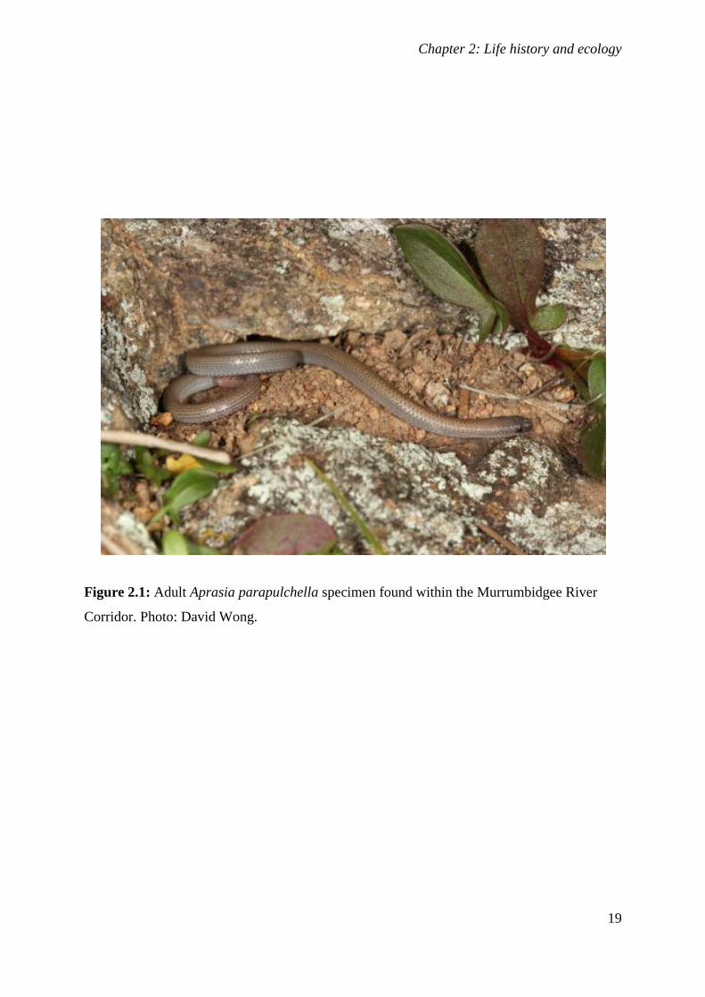
Figure 2.1: Adult Aprasia parapulchella specimen found within the Murrumbidgee River Corridor. Photo:
David Wong................................................................................................................................... 19
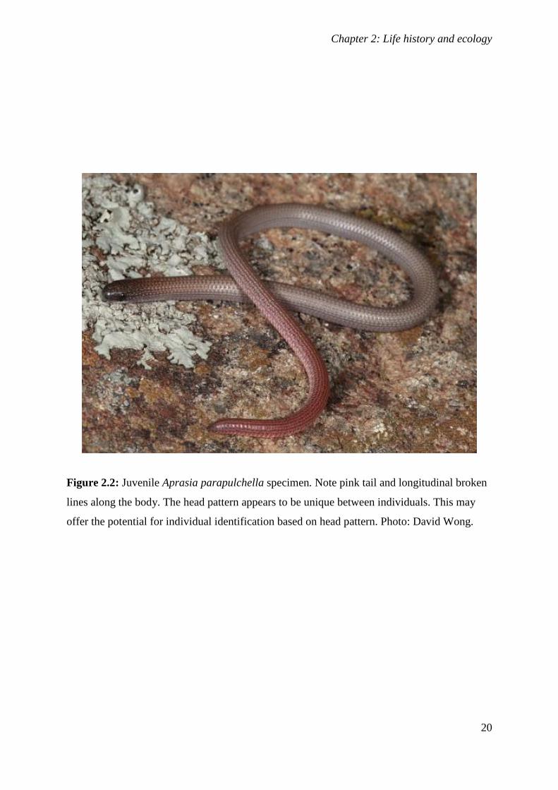
Figure 2.2: Juvenile Aprasia parapulchella specimen. Note pink tail and longitudinal broken lines along the
body. The head pattern appears to be unique between individuals. This may offer the potential for
individual identification based on head pattern. Photo: David Wong. .......................................... 20
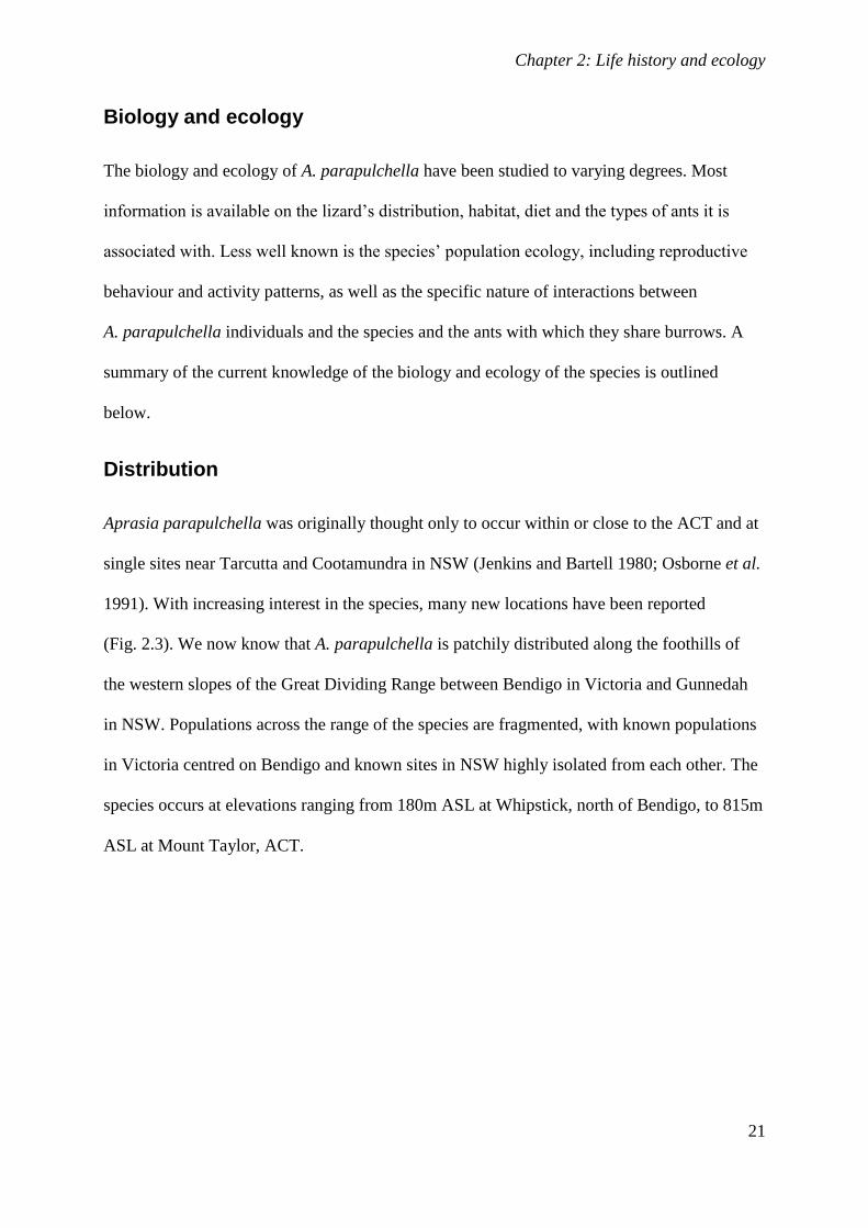
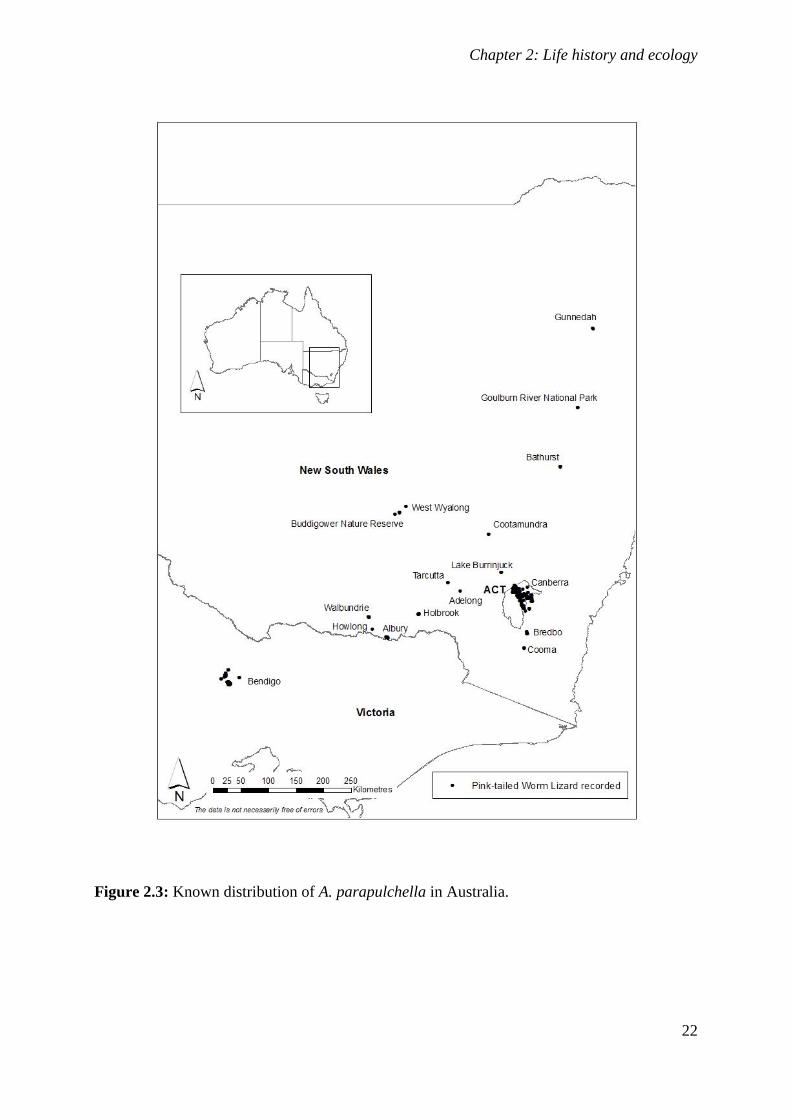
Figure 2.3: Known distribution of A. parapulchella in Australia. ........................................................... 22
Figure 2.4: Known distribution of A. parapulchella in the ACT. ............................................................ 23
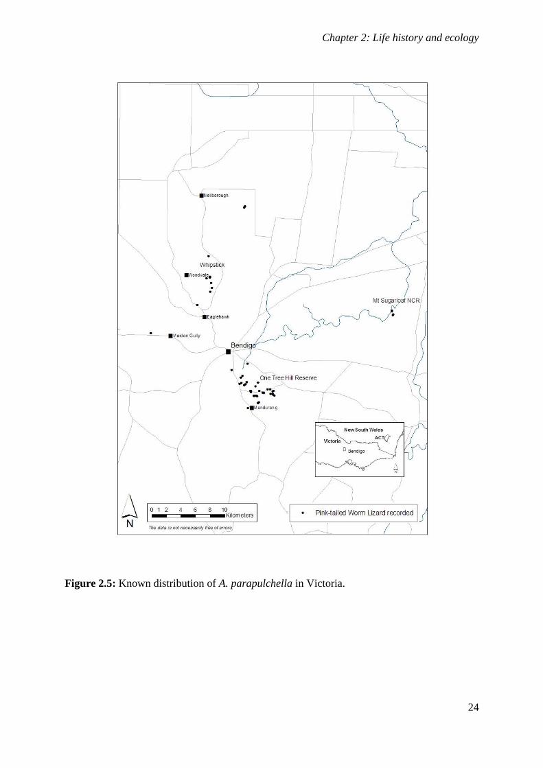
Figure 2.5: Known distribution of A. parapulchella in Victoria. ............................................................. 24
Figure 2.6: Typical high quality habitat suitable for A. parapulchella located at the type locality (Coppins
Crossing, ACT). There is a high cover of lightly embedded surface rock. The ground layer vegetation is
relatively intact with Kangaroo Grass (Themeda australis) present. Other forbs such as Creamy Candles
(Stackhousia monogyna) and sedges (Lomandra spp.) can be made out. Note that this site does exhibit
some weed invasion from Blackberry (Rubus fruticosus) and Mullein (Verbascum species). Photo: David
Wong. ............................................................................................................................................ 31
Figure 2.7: Pink-tailed Worm-lizard habitat at Albury. Photo: Damian Michael. ................................... 34
Figure 2.8: Pink-tailed Worm-lizard habitat in the Whipstick area of the Greater Bendigo National Park. The
vegetation at this site is dominated by Mallee species and there is no evidence of surface rock. Photo:
Peter Robertson. ............................................................................................................................ 37
Figure 2.9: Adult A. parapulchella specimen found beneath a rock. The ant galleries that the species utilises are
evident in the photo. Photo: David Wong. .................................................................................... 39
Figure 2.10: An example of a sloughed A. parapulchella skin found underneath a rock. Photo: David Wong.
....................................................................................................................................................... 40
Figure 3.1: Map of the study area showing known records of occurrence of Aprasia parapulchella in the
Australian Capital Territory and surrounding areas. ..................................................................... 59
Figure 3.2: Visual representation of the MaxEnt model predicting habitat for A. parapulchella in the Australian
Capital Territory. ........................................................................................................................... 66
Figure 3.3: Predicted likelihood of occurrence of A. parapulchella in association with soil groups in the
Australian Capital Territory and surrounds. The light bars indicate the marginal response of the logistic
likelihood of the model when the soil variable is varied and all other variables are kept at their sample
average. The dark bars indicate the individual response (i.e. a MaxEnt model created using only the soil
variable). The error bars indicate one standard deviation either side of the mean. ....................... 69
Figure 3.4: Predicted likelihood of occurrence of A. parapulchella in association with geology in the Australian
Capital Territory and surrounds. The light bars indicate the marginal response of the logistic likelihood of
the model when the geology variable is varied and all other variables are kept at their sample average.
The dark bars indicate the individual response (i.e. a MaxEnt model created using only the geology
variable). The error bars indicate one standard deviation either side of the mean. ....................... 70
Figure 3.5: Predicted likelihood of occurrence of A. parapulchella as a function of slope in the Australian
Capital Territory and surrounds. The light line indicates the marginal response of the logistic likelihood of
the model when the slope variable is varied and all other variables are kept at their sample average. The
dark line indicates the individual response (i.e. a MaxEnt model created using only the slope variable).
The error bars indicate one standard deviation either side of the mean. ........................................ 71
List of Figures
xxiv
Figure 3.6: Predicted likelihood of occurrence of A. parapulchella as a function of average minimum
temperature in October in the Australian Capital Territory and surrounds. The light line indicates the
marginal response of the logistic likelihood of the model when the temperature variable is varied and all
other variables are kept at their sample average. The dark line indicates the individual response (i.e. a
MaxEnt model created using only the temperature variable). The error bars indicate one standard
deviation either side of the mean. .................................................................................................. 72
Figure 3.7: Predicted likelihood of occurrence of A. parapulchella as a function of average rainfall in October in
the Australian Capital Territory and surrounds. The light line indicates the marginal response of the
logistic likelihood of the model when the rainfall variable is varied and all other variables are kept at their
sample average. The dark line indicates the individual response (i.e. a MaxEnt model created using only
the rainfall variable). The error bars indicate one standard deviation either side of the mean. ..... 73
Figure 3.8: Predicted likelihood of occurrence of A. parapulchella in association with the agricultural
modification variable in the Australian Capital Territory and surrounds. The light bars indicate the
marginal response of the logistic likelihood of the model when the agricultural modification variable is
varied and all other variables are kept at their sample average. The dark bars indicate the individual
response (i.e. a MaxEnt model created using only the agricultural modification variable). The error bars
indicate one standard deviation either side of the mean. ............................................................... 74
Figure 4.1: Map showing location of study area and occurrence records used in MaxEnt modelling. The sub-area
where the models were separately tested and the grid of points used for testing is also shown. ... 93
Figure 4.2: Percentage area predicted according to vegetation classes for MaxEnt models of predicted
occurrence of A. parapulchella with and without agricultural modification. .............................. 103
Figure 4.3: Difference plot of area predicted according to vegetation class for MaxEnt models of predicted
occurrence of A. parapulchella with and without agricultural modification. .............................. 104
Figure 4.4: Comparison of thresholded MaxEnt model without (A) and with (B) the agricultural modification
variable included at a location where potential habitat for A. parapulchella was mapped in the field using
expert knowledge of habitat requirements. The models were converted to presence/absence predictions by
using the threshold selected by MaxEnt that maximised specificity (equal training sensitivity and
specificity; threshold = 0.32 [agricultural modification included] and 0.341 [agricultural modification
excluded]) [depicted in light grey] and an arbitrary threshold of 0.5 (depicted in dark grey). White areas
indicate areas not predicted as suitable by either of the models. A. parapulchella specimens were found
throughout the area depicted........................................................................................................ 109
Figure 5.1: Study area and location of the 29 study sites in the Australian Capital Territory. ............... 126
Figure 5.2: Plots of fitted functions for the boosted regression tree model showing the response of the abundance
of A. parapulchella to each of the explanatory variables. The percentages shown in brackets next to the
explanatory variable titles on the x-axes refer to the percentage of the total deviance of the model
explained by the variable. ............................................................................................................ 133
Figure 5.3: Perspective plot showing the response of number of specimens of A. parapulchella to percentage
cover of species from the ‘large tussock species’ functional group and floristic value score. .... 134
Figure 6.1: Hypothesised response of Aprasia parapulchella to various states within McIntyre and Lavorel’s
(2007) state-and-transition model. [Adapted from McIntyre and Lavorel (2007)]. The model represents
five land use types in temperate eucalypt grassy woodlands of south-eastern Australia. The states
(numbered 1 – 5) are described in terms of the general level of grazing, soil disturbance and soil fertility
associated with each particular state. The management associated with the maintenance of the state is
illustrated using circular arrows and straight arrows correspond with the transitions between states. Of
considerable interest is the response of the species at transitional parts of this diagram............. 149
List of Tables
xxv
List of Tables
Table 2.1: Mean and range of snout-vent lengths for different age-classes of
A. parapulchella in the ACT (adapted from Jones 1999). ..................................................... 42
Table 2.2: Comparison of mean snout-vent length and mean weight of male and female
A. parapulchella specimens captured in the ACT and Victoria and results of t-
tests. ....................................................................................................................................... 43
Table 3.1: Average model evaluation results for 10 replicate runs of MaxEnt model for
Aprasia parapulchella in the Australian Capital Territory using 168 data points
for training and 168 data points for testing. The training and testing data were
randomly partitioned by MaxEnt. .......................................................................................... 64
Table 3.2: Estimates of the relative contribution of each of the variables included in a
MaxEnt model of predicted occurrence of A. parapulchella in the Australian
Capital Territory. The first estimate is obtained by adding or subtracting (if the
lambda value is negative) the absolute value of increase or decrease in
regularized training gain to the contribution of the variable in each iteration of the
training algorithm, in each iteration of the training algorithm.. The second
estimate is derived by randomly permuting the values on training presence and
background data for each variable in turn. The permuted data is used to re-
evaluate the model. The resulting drop in training AUC, normalized to
percentages, is shown. Values shown are averages over replicate runs. As there is
inter-correlation amongst the variables, the values should interpreted with
caution. ................................................................................................................................... 68
Table 4.1: Area under the receiver operating curve (AUC) and gain values for MaxEnt
model for Aprasia parapulchella in the Australian Capital Territory with and
without the agricultural modification layer incorporated. .................................................... 101
Table 4.2: Percentage contribution of variables in species distribution models for
Aprasia parapulchella with and without agricultural modification. .................................... 102
Table 4.3: Results of the Welch two-sample t-test comparing mean predicted probability
of presence for models with and without agricultural modification included using:
a) records from an area of approximately 6 km x 7 km area which contained a
range of levels of agricultural disturbance and; b) a regular grid of points from the
same area. ............................................................................................................................. 105
Table 4.4: Model evaluation figures derived from confusion matrices for
presence/absence models with and without the agricultural modification variable
included in the approximately 6km x 7km sub-area. The performance of the
models was assessed based on 74 presence points and a regular grid of 133 points
that was biased towards likely absence by excluding mapped habitat in the study
areas. Figures are given for models using the threshold for presence suggested by
MaxEnt that maximised model specificity as well as for an arbitrary presence
threshold of 0.5. ................................................................................................................... 107
Table 5.1: Summary statistics for the BRT analysis using the default 10-fold cross
validation with a tree complexity of 3, learning rate of 0.001 and bag fraction of
0.9 (See online tutorial accompanying Elith et al. for a detailed explanation of the
modelling procedure). .......................................................................................................... 132
Chapter 1: Introduction
1
1. Introduction
Background
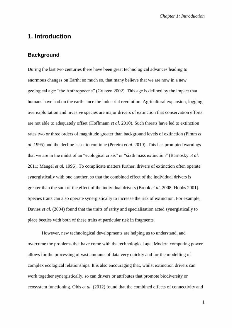
During the last two centuries there have been great technological advances leading to
enormous changes on Earth; so much so, that many believe that we are now in a new
geological age: “the Anthropocene” (Crutzen 2002). This age is defined by the impact that
humans have had on the earth since the industrial revolution. Agricultural expansion, logging,
overexploitation and invasive species are major drivers of extinction that conservation efforts
are not able to adequately offset (Hoffmann et al. 2010). Such threats have led to extinction
rates two or three orders of magnitude greater than background levels of extinction (Pimm et
al. 1995) and the decline is set to continue (Pereira et al. 2010). This has prompted warnings
that we are in the midst of an “ecological crisis” or “sixth mass extinction” (Barnosky et al.
2011; Mangel et al. 1996). To complicate matters further, drivers of extinction often operate
synergistically with one another, so that the combined effect of the individual drivers is
greater than the sum of the effect of the individual drivers (Brook et al. 2008; Hobbs 2001).
Species traits can also operate synergistically to increase the risk of extinction. For example,
Davies et al. (2004) found that the traits of rarity and specialisation acted synergistically to
place beetles with both of these traits at particular risk in fragments.
However, new technological developments are helping us to understand, and
overcome the problems that have come with the technological age. Modern computing power
allows for the processing of vast amounts of data very quickly and for the modelling of
complex ecological relationships. It is also encouraging that, whilst extinction drivers can
work together synergistically, so can drivers or attributes that promote biodiversity or
ecosystem functioning. Olds et al. (2012) found that the combined effects of connectivity and
Chapter 1: Introduction
2
reserve protection led to a doubling of the biomass of roving herbivorous fish on protected
reefs near mangroves. This, in turn, led to a trophic cascade, reducing algal cover and
promoting coral recruitment. Viewed in this light, it is evident that the future trajectory of
many species will depend heavily on the extent to which extinction drivers continue unabated
as well as the extent to which drivers of optimum ecosystem function are maintained or
restored.
This thesis is very much concerned with this dual nature of technology and the
Anthropocene. The focal species is a lizard (the Pink-tailed Worm-lizard Aprasia
parapulchella) that has become threatened as a result of anthropogenic impacts on its key
habitat resources (Wong et al. 2011). Its future depends on arresting extinction drivers and
promoting drivers that restore its habitat. Throughout this thesis, I draw on technological
advances that allow the characterisation of complex relationships and can shed light on the
factors important for its continued survival. The technology also allows spatially explicit
predictions of occurrence that may inform the future conservation of the species. It is but one
example in the sea of threatened species that grows by the day (Hoffmann et al. 2010). I hope
that the information will be useful, not only for this species, but also others.
Species Distribution Models
In order to conserve or manage species, it is important to have a good understanding of where
they occur. Species distribution models (SDMs) aim to predict the distribution of a particular
species or group of species. In general, SDMs predict where a species is likely to occur based
on a range of environmental attributes that are assumed to influence the occurrence of the
species, thereby characterising the environmental conditions that are suitable for the species
(Pearson 2007). In recent years the use of species distribution models has steadily increased.
Consequently, a great variety of modelling techniques have been developed (Elith et al. 2006;
Chapter 1: Introduction
3
Guisan and Thuiller 2005) and SDMs have been applied in a wide range of scenarios in the
fields of ecology, conservation biology, and evolutionary biology (Miller 2010; Pearson 2007;
Thuiller et al. 2008). Some of the applications in conservation biology include: identifying
new areas for survey especially for rare species (Bourg et al. 2005; Guisan et al. 2006a;
Raxworthy et al. 2003), identifying possible sites for re-introduction of threatened species
(Pearce and Lindenmayer 1998) and prioritising areas for reserve or species conservation
(Ferrier et al. 2002).
The importance of niche
The concept of niche (Chase and Leibold 2003) is central to the field of ecology as it
describes the environmental space in which organisms can exist (either theoretically or in
reality). Species distribution models aim to encapsulate this niche and represent it in
geographical space. There have been many different attempts to characterise niche (Sillero
2011). Hutchinson (1957) identified two aspects of ecological niche. The fundamental niche
was described as the full range of environmental conditions under which an organism can
persist. Thus it is a theoretical range of physiological tolerance of an organism within
environmental space unmediated by the effects of biotic interactions (e.g. intra-specific
competition or predation). The realised niche is within the bounds of the fundamental niche
but takes into account biotic interactions. Pearson (2007) introduced the term “occupied
niche” which includes biotic interactions but also the geographical and historical constraints
that result in an organism not occupying all suitable habitat (e.g. geographical barriers to
dispersal, insufficient time for dispersal, human modification, etc.), though one could argue
that human modification could technically fit under Hutchinson’s model as a form of intra-
specific competition.
Chapter 1: Introduction
4
SDMs attempt to represent the occupied niche of a species in geographical space.
Therefore, the extent to which they can successfully incorporate the factors that are affecting
the distribution of the species will determine how close the models come to achieving this
goal. For this reason, there has been some discussion in the scientific literature on the
importance of SDMs incorporating ecological realism by accounting for processes such as
migration, geographical barriers and disturbance factors (Austin 2007; Austin 2002; Hampe
2004; Hirzel and Le Lay 2008; Pearson and Dawson 2004). Thus, determining whether
models simulate fundamental, realised (or occupied) niche is important in order to
acknowledge whether a given model predicts a theoretical physiological distribution or a
distribution based on observations in the field (Guisan and Zimmermann 2000; Pearson
2007).
Model types and usage
A large range of methods are available for people wanting to develop SDMs. Species
distribution models may be divided into those that use presence records only (presence-only
methods) and those that use presence records and also characterise the background with a
sample of known or generated absence points [presence/absence methods] (Elith et al. 2006;
Ferrier et al. 2002). Some methods, such as generalized additive models (GAMs) (Hastie and
Tibshirani 1986), generalized linear models (GLMs) and artificial neural networks(ANNs)
require data on where a species has been recorded as absent, whilst others, such as Maxent
relate the environment where a species is known to occur to other parts of the study area to
produce a ‘background’. Where a ‘background’ is generated, occurrence sites are also
included in the ‘background’ (Pearson 2007). Presence/absence algorithms can also use
‘pseudo-absences’ generated randomly or using weighting criteria (Engler et al. 2004;
Stockwell and Peters 1999) Some techniques, known as community-based techniques model
the distribution of a number of species at once.
Chapter 1: Introduction
5
BIOCLIM and DOMAIN are examples of SDMs that use only presence records. BIOCLIM
generates a bioclimatic envelope for the species and DOMAIN is a distance-based method
that assesses new sites in terms of their environmental similarity to sites where the species is
known to be present (Elith et al. 2006).
Of the presence/absence methods, GLM and GAM have, traditionally, often been often used
due to their ability to model ecological relationships in a realistic way (Austin 2002; Elith et
al. 2006). Generalised additive models are able to model complex ecological response shapes
through the use of non-parametric, data-defined smothers to fit non-linear functions, whereas
GLMs fit parametric terms (usually linear quadratic or cubic functions) and are therefore less
flexible than GAMs (Elith et al. 2006). GRASP (Lehmann et al. 2002) is an example of a
modelling package that uses regression analysis for species distribution modelling. It may be
implemented through the Splus or R statistical packages (Guisan et al. 2006b). Other models
such as BRUTO and multivariate adaptive regression splines (MARS) are either variations or
enhancements of regression techniques (Elith et al. 2006).
Machine learning techniques are an alternative to regression techniques and include
ANNs and Decision Tree based methods. Artificial neural networks and CART can fit robust
models to ecological data and may be better than GAM and GLM at modelling interactions
but do not allow for observation of ecological response curve shapes and do not select
variables based on the appropriate statistical distributions (Lehmann et al. 2002) . Genetic
algorithm models such as GARP use genetic algorithms to select sets of rules that best predict
the distribution of a species. Recent developments in SDM have produced new powerful
methods based on machine learning including boosted regression trees (BRT) and Maxent
that have been shown to outperform the more traditional methods (Elith et al. 2006).
Chapter 1: Introduction
6
MaxEnt attempts to estimate a probability distribution for the occurrence of a species
within a geographical space from known occurrence data and environmental variables or
“features” (Phillips et al. 2006). MaxEnt compares probability densities in covariate space,
deriving the “implied” conditional probability of occurrence (termed the “logistic output”)
from the relationship between the conditional density of the covariates at the presence sites
and the unconditional (“marginal”) density of covariates across the study area (2011). The
conditional probability is “implied” as the prevalence of the species is required to derive the
actual conditional probability of occurrence. However, presence-only techniques cannot
derive this figure, so the prevalence must be estimated or the default of 0.5 used (Elith et al.
2011). For a more detailed statistical explanation of MaxEnt, see Elith et al. (2011). MaxEnt
is commonly used because it allows for the use of presence-only data, can incorporate
categorical and continuous data, can incorporate interactions between variables, uses a
process called l-regularization to avoid over-fitting and can be used with small sample sizes
(Hernandez et al. 2006; Phillips et al. 2006). Disadvantages of the method include that it is
less mature than regression methods such as GLM and GAM; the effectiveness of
regularization processes that aim to avoid over-fitting requires further evaluation;
extrapolation in time and space must be done with caution and; like other presence-only
methods, the method is more sensitive to sampling bias than presence/absence methods (Elith
et al. 2011).
Some modelling packages offer a number of different modelling techniques within the
one package. BIOMOD (Thuiller 2003) implements a number of modelling techniques
including GLMs, GAMs, classification and regression tree analysis (CART), artificial neural
networks (ANN), Boosted Regression Trees (BRT) and a number of other techniques (Guisan
et al. 2006b).
Chapter 1: Introduction
7
Presence/absence or presence-only?
In general, where presence/absence data are available, it is preferable to use presence/absence
methods (e.g. GLMs, GAMs or ensemble methods of regression trees such as BRT or random
forests) as they are less susceptible to the effects of sample selection bias than presence-only
models (Elith et al. 2011). However, these data are only available in cases when there has
been a systematic survey to confirm presence or abundance and absence. In many cases, there
has been no such systematic survey undertaken, so presence-only methods are appropriate. A
major advantage of presence /absence models over presence-only models is their better ability
to estimate the prevalence of a species in the landscape than presence-only models, but they
are still not immune to problems such as imperfect detection.
Are the times a changing?
Modelling can broadly be split into two types: traditional data modelling, that is based on a
data model and; algorithmic modelling or machine learning, that relies on algorithmic models
and assumes that the data mechanism is unknown (Breiman 2001). Examples of data
modelling include logistic and linear regression, whilst examples of machine learning include
neural networks and decision trees (Breiman 2001). Within the context of species distribution
modelling, GLM and GAM are examples of techniques that rely on a data model and machine
learning methods such as MaxEnt, BRT and CART are examples of techniques which rely on
algorithms to learn relationships between the response variable and predictors (Elith et al.
2008). Therefore, the predictive ability of the model is emphasised in machine learning along
with what is being predicted and how to measure predictive success (Elith et al. 2008).
The traditional regression-based statistical approach focuses on what model will be postulated
(e.g. are there interactions), the distribution of the response and whether observations are
independent; whereas the machine learning approach assumes a complex and unknown data-
Chapter 1: Introduction
8
generating process (i.e. nature in the case of ecology) and attempts to learn the response,
identifying dominant patterns through observations of inputs and responses (Elith et al. 2008)
Whilst methods that rely on data model have been by far the most prevalent methods of
choice in the statistical community, often because researchers are uncomfortable about what
they perceive as the “black box” nature of machine learning, Breiman (2001) suggests that
this has limited the field of statistics and led to, in some cases, irrelevant theory and
questionable conclusions. Machine learning methods are gaining popularity in the species
distribution modelling community as they often outperform more traditional methods in
predictive ability (Elith et al. 2006; Elith et al. 2008). In addition, methods at the forefront of
machine learning such as BRT are attractive to ecologists as they can fit complex non-linear
relationships, deal with interactions between variables and are well suited for modelling with
large sets of predictors (Elith et al. 2008).
The case study of a threatened species in a changing world
The Pink-tailed Worm-Lizard A. parapulchella is a threatened species that has
declined across its range. It is almost certain that the majority of this decline is a result of
agricultural activities leading to changes to the key habitat features on which the species
depends (Jones 1999; Langston 1996). There have been several investigations that have
considered the effect of disturbance on A. parapulchella (Jones 1992; Jones 1999; Osborne et
al. 1991; Osborne and McKergow 1993). Jones (1999) suggested that further work in this area
be undertaken to clarify the relationship between A. parapulchella and disturbance. For this
reason and the pressing nature of the problem in the global context, I have chosen to make
agricultural disturbance and its relevance to A. parapulchella a key theme running through the
thesis. A considerable amount of the literature on A. parapulchella is contained only in
academic theses and technical reports. This is a considerable barrier to providing increased
Chapter 1: Introduction
9
access to the knowledge about this species. Therefore, another objective in this thesis is,
through publication of a review, to add to and synthesise the existing knowledge of the
species distribution and ecology in order to inform conservation efforts.
A. parapulchella was not described until 1974 (Kluge 1974), thirty years after a
considerable increase in post-war land clearing and pasture improvement through application
of superphosphate commenced in south-eastern Australia. By this time, the species would
already have undergone considerable declines and range contractions as a result of these
activities and more generally through increases in agricultural activity, forestry and urban
development. These are the three major sources of habitat loss and decline in the Australian
Capital Territory (ACT). Therefore, the future trajectory of the species is likely to be highly
dependent on the extent to which these threats are constrained or otherwise. For example, the
species has recently been subject to development pressure in an extensive part of the
Molonglo Valley in the ACT (Osborne and Wong 2010; Wong and Osborne 2010). Future
population growth is likely to put further pressure on populations of A. parapulchella in the
ACT.
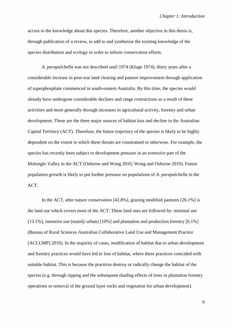
In the ACT, after nature conservation [42.8%], grazing modified pastures [26.1%] is
the land use which covers most of the ACT. These land uses are followed by: minimal use
[13.1%], intensive use (mainly urban) [10%] and plantation and production forestry [6.1%]
(Bureau of Rural Sciences Australian Collaborative Land Use and Management Practice
[ACLUMP] 2010). In the majority of cases, modification of habitat due to urban development
and forestry practices would have led to loss of habitat, where these practices coincided with
suitable habitat. This is because the practices destroy or radically change the habitat of the
species (e.g. through ripping and the subsequent shading effects of trees in plantation forestry
operations or removal of the ground layer rocks and vegetation for urban development).

Chapter 1: Introduction
10
Whilst agricultural activities have undoubtedly led to modification of the habitat of
A. parapulchella and, in some cases, habitat destruction, the impacts of agricultural
modification are often less severe than those of forestry or urban development. Therefore, the
portion of land under agricultural leases represents a sizable area of potentially suitable
habitat for the species. Even though there is little information on the extent to which this land
is suitable or occupied, it is likely that many areas could be very important in the future
conservation of the species, complementing habitat on reserved land. For this reason,
determining the extent to which these landscapes are occupied and subsequent management of
these areas are likely to be important factors with respect to the future conservation of
A. parapulchella. Grazing of modified pastures is the major land use across the range of the
species (Bureau of Rural Sciences Australian Collaborative Land Use and Management
Practice [ACLUMP] 2009). It is therefore highly likely that grazing, and practices associated
with grazing (e.g. pasture sowing and fertiliser addition), have been major contributors to the
loss and decline of A. parapulchella across its distributional range. Of considerable interest
(but unknown) is the extent to which rocks have been removed from landscapes that support,
or once supported, A. parapulchella in association with these practices.
It is believed that the nature of the land tenure system may have been a reason for the
higher number of records of A. parapulchella in the ACT (Jones 1999; Langston 1996). There
is no freehold land in the ACT and, until recently, all rural leases were short-term, giving
landholders little security of tenure and less incentive to intensify practices or increase input
of fertiliser than in other states (Langston 1996). This idea requires further testing and
analysis before firm conclusions can be drawn. For example, it may be the case that fertiliser
application, a shorter term solution to increasing stocking densities, would have been
favoured over the longer-term and more expensive investment of pasture sowing. The
influence of the habitat type is also worthy of exploration. A. parapulchella is associated with
Chapter 1: Introduction
11
rocky, and therefore, less arable land. This is likely to have influenced the decisions of
landholders. Further research in relation to these important aspects of land use history is
therefore warranted. Since 2000, certain rural leases have been able to apply for 99 year leases
(G. Hirth, ACT Parks Conservation and Lands, pers. comm.). This gives leaseholders who
take up such a lease term a much higher level of security of tenure (the same lease term as
urban residents). Therefore, the probability that landholders will wish to increase inputs (such
as application of fertiliser) and intensify practices is increased. This is likely to be detrimental
for the conservation of species such as A. parapulchella, as well as for landscape function
(McIntyre and Tongway 2005). Within this context, a good understanding of the factors
important for the conservation of the A. parapulchella is needed in order to best inform
conservation efforts. Knowledge of the likely occurrence of the species will also inform future
conservation planning and management and help to identify key areas for protection. Whilst
the focus is local, it is envisaged that the approaches could be applied at a range of scales to
other species.

Chapter 1: Introduction
12
Aims and structure of this thesis
My broad aims in this thesis are to increase our understanding of the factors affecting the
distribution of A. parapulchella in the ACT and to determine the influence of agricultural
disturbance in influencing its distribution. I address these aims using species distribution
modelling at the scale of the ACT and by investigating factors affecting the abundance of
A. parapulchella at the patch scale.
My specific objectives are to:
I) describe the environmental correlates of occurrence of A. parapulchella in the
ACT (Chapter 3)
II) construct an SDM of the predicted occurrence of A. parapulchella in the ACT
(Chapter 3)
III) determine whether adding agricultural modification improves an SDM of the
predicted occurrence of A. parapulchella in the ACT (Chapter 4)
IV) estimate the impact of agricultural modification on the habitat of A. parapulchella
in the ACT (Chapter 4)
V) determine the factors affecting the occurrence and abundance of A. parapulchella
at the patch scale (Chapter 5)
VI) synthesise the existing knowledge of A. parapulchella and integrate my findings
into the current pool of knowledge (Chapter1; Chapter 6)
The chapters in this thesis (excluding Chapter 1 and Chapter 6) are set out as a series
of manuscripts; therefore, some repetition is unavoidable. However, I have endeavoured to
minimise duplication as much as possible. Each of the chapters (excluding the introduction
and synopsis) is set out as a stand-alone publication that includes an Abstract, Introduction,
Chapter 1: Introduction
13
Methods, Results and Discussion. The literature cited in each chapter has been combined into
a single reference list at the end of the thesis. Whilst I have received valuable advice and
editorial comments from the co-authors of the manuscripts, I conceived the ideas, conducted
the field work, undertook the analyses and wrote and edited the manuscripts.
The thesis structure is outlined below:
In Chapter 2, the existing information available on A. parapulchella is synthesised. In
addition, data on body size in Victoria and the ACT are analysed. This chapter has been
published as:
Wong D. T. Y., Jones S. R., Osborne W. S., Brown G. W., Robertson P., Michael D.
R. & Kay G. M. (2011) The life history and ecology of the Pink-tailed Worm-lizard Aprasia
parapulchella Kluge - a review. The Australian Zoologist 35, 927-40 (Appendix 1).
In Chapter 3, the distribution of A. parapulchella in the ACT region is modelled using species
distribution modelling and the response of the variables examined.
This manuscript will be submitted as:
Wong D. T. Y., Gruber B., Sarre S. D. & Osborne W. S. Clarifying environmental correlates
of occurrence for Aprasia parapulchella using MaxEnt.
Chapter 4 focuses on the contribution of agricultural modification in the MaxEnt
model constructed in Chapter 3. Models with and without the agricultural modification
variable included are compared in order to determine the importance of including agricultural
modification into a species distribution model for A. parapulchella.
Chapter 1: Introduction
14
This manuscript will be submitted as:
Wong D. T. Y., Gruber B., Sarre S. D. & Osborne W. S. Species distribution modelling for a
disturbance-sensitive lizard: agricultural modification counts.
In Chapter 5, the habitat factors important for A. parapulchella are analysed using
boosted regression trees (BRT), a relatively recent statistical method. I examine whether
vegetation indicators of disturbance are a good predictor of the occurrence and abundance of
A. parapulchella and identify which habitat factors are most influential in determining
occupancy at the patch scale.
This manuscript will be submitted as:
Wong D. T. Y., Gruber B., Sarre S. D. & Osborne W. S. Factors affecting the occurrence of a
threatened legless-lizard at the patch scale.
The final chapter of the thesis brings together the key findings of my research within the
context of conservation in the 21st century for both A. parapulchella and species in general. I
discuss applications for the research and identify further avenues for investigation.
Chapter 2: Life history and ecology
15
2. The life history and ecology of the Pink-tailed Worm-
lizard (Aprasia parapulchella) Kluge – a review1
Abstract
This review synthesises research on the Pink-tailed Worm-lizard Aprasia parapulchella - a
threatened species with life-history traits and habitat and dietary preferences that make it
particularly vulnerable to decline. Further information on the ecology of A. parapulchella is
required in order to develop effective approaches to conservation and management,
particularly given the conservation status of the species. Aprasia parapulchella is a dietary
specialist living in the burrows of a number of species of small ants, the eggs and larvae of
which it preys upon. It is late maturing, has a small clutch, is thought to be long-lived and has
specific habitat preferences. It has a strong association with landscapes that are characterised
by outcroppings of lightly-embedded surface rocks. The lizard is associated with a particular
suite of ant species and ground cover tending towards open native vegetation (grasses and
shrubs) at most sites, but with regional differences. Although the highest densities have been
recorded in areas without tree cover, the species has also been found in clearings in open-
forest and woodland. The relative density of populations and the snout-vent length and weight
of specimens reveal regional differences, suggesting that further analysis of the genetic status
1 This manuscript has been published as: Wong D. T. Y., Jones S. R., Osborne W. S., Brown G. W., Robertson P.,
Michael D. R. & Kay G. M. (2011) The life history and ecology of the Pink-tailed Worm-lizard Aprasia parapulchella Kluge
- a review. The Australian Zoologist 35, 927-40. Whilst I have received valuable advice and editorial comments from the co-
authors of the manuscripts, I conceived the ideas, conducted the field work, undertook the analyses and wrote and edited the
manuscript. The published article is included in Appendix 1. There are some minor differences between the published paper
and this thesis chapter as some examiner’s comments have been addressed subsequent to publication.
Chapter 2: Life history and ecology
16
of the population across its range is warranted. There is still much to learn about the ecology
of the species, particularly with respect to movement, breeding, dispersal and the relationship
between lizards and ants. Further survey for new populations remains a key priority.
Introduction
The genus Aprasia (Pygopodidae) is a geographically dispersed and highly fragmented group
with small populations distributed mostly in mesic-temperate areas of Australia that receive
high winter rainfall (Jennings et al. 2003). The Pink-tailed Worm-lizard Aprasia
parapulchella is the most south-easterly occurring species of the genus and is distributed
along the western foothills of the Great Dividing Range between Bendigo in Victoria and
Gunnedah in northern New South Wales (NSW) (Fig. 3). It is an intriguing species by virtue
of its distinctive morphology, fossorial habits and unusual life-history, which involves co-
habitation in the burrows of small ants, the eggs and larvae of which it preys on. Its life-
history traits (late-maturing, low reproductive rate, likely low vagility) and specific habitat
and dietary requirements make it sensitive to landscape change (Davies et al. 2004; Purvis et
al. 2000). Known and potential threats to the species include pasture improvement,
overgrazing, soil disturbance, rock removal, weed invasion, inappropriate fire regimes and
fire management activities, recreational activities and predation. The species is listed as
threatened in each state in which it occurs as well as nationally. It has been assigned
‘vulnerable’ status nationally (Environment Protection and Biodiversity Conservation Act
1999), in the Australian Capital Territory (ACT) (Nature Conservation Act 1980) and in NSW
(Threatened Species Conservation Act 1995) and ‘endangered’ status in Victoria (Flora and
Fauna Guarantee Act 1988). Therefore, a comprehensive understanding of the life history,
ecology and distribution of the species is essential for future conservation efforts.
Chapter 2: Life history and ecology
17
There have been several investigations into the distribution, ecology and conservation
of A. parapulchella since its description (Appendix 2). However, almost all of this
information is contained in technical reports or theses and is not readily accessible. It is
critical that this information be made more widely available and that knowledge gaps are
identified. Therefore, the aim of this review is to synthesise available biological and
ecological information and identify areas for future research.
Taxonomy and morphology
Aprasia parapulchella (Fig. 2.1; Fig. 2.2), one of the 12 species in the genus, belongs to the
family Pygopodidae (flap-footed lizards) (Wilson and Swan 2008). A. parapulchella was
described by Kluge in 1974 from 20 specimens collected at Coppins Crossing (the type
locality) in the ACT and one specimen from Tarcutta, NSW (Osborne et al. 1991).
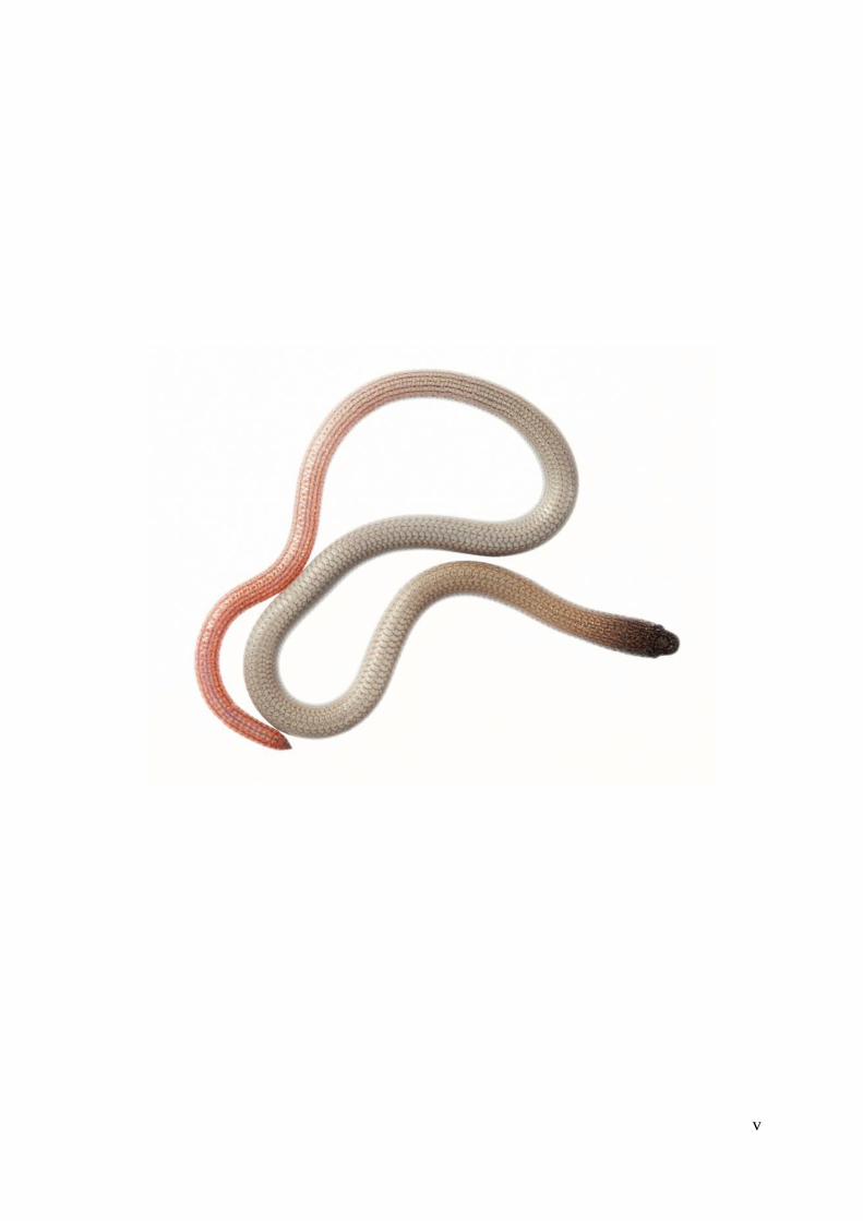
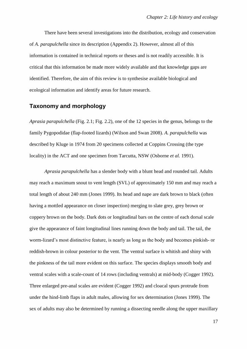
Aprasia parapulchella has a slender body with a blunt head and rounded tail. Adults
may reach a maximum snout to vent length (SVL) of approximately 150 mm and may reach a
total length of about 240 mm (Jones 1999). Its head and nape are dark brown to black (often
having a mottled appearance on closer inspection) merging to slate grey, grey brown or
coppery brown on the body. Dark dots or longitudinal bars on the centre of each dorsal scale
give the appearance of faint longitudinal lines running down the body and tail. The tail, the
worm-lizard’s most distinctive feature, is nearly as long as the body and becomes pinkish- or
reddish-brown in colour posterior to the vent. The ventral surface is whitish and shiny with
the pinkness of the tail more evident on this surface. The species displays smooth body and
ventral scales with a scale-count of 14 rows (including ventrals) at mid-body (Cogger 1992).
Three enlarged pre-anal scales are evident (Cogger 1992) and cloacal spurs protrude from
under the hind-limb flaps in adult males, allowing for sex determination (Jones 1999). The
sex of adults may also be determined by running a dissecting needle along the upper maxillary
Chapter 2: Life history and ecology
18
surface (upper surface of the jaw), with males possessing a rough maxillary surface. However,
this method is more invasive than checking for cloacal spurs and is not the preferred method
for determining gender (Jones 1992; Jones 1999).
Aprasia parapulchella can be separated from all other species of Aprasia in eastern
Australia by the following combination of characters: (1) the first upper labial scale is wholly
fused with the nasal scale, (2) three pre-anal scales are present, (3) two pre-ocular scales are
usually present, and (4) there is an absence of a lateral head pattern (Cogger 1992; Wilson and
Swan 2008).
Chapter 2: Life history and ecology
19
Figure 2.1: Adult Aprasia parapulchella specimen found within the Murrumbidgee River
Corridor. Photo: David Wong.
Chapter 2: Life history and ecology
20
Figure 2.2: Juvenile Aprasia parapulchella specimen. Note pink tail and longitudinal broken
lines along the body. The head pattern appears to be unique between individuals. This may
offer the potential for individual identification based on head pattern. Photo: David Wong.
Chapter 2: Life history and ecology
21
Biology and ecology
The biology and ecology of A. parapulchella have been studied to varying degrees. Most
information is available on the lizard’s distribution, habitat, diet and the types of ants it is
associated with. Less well known is the species’ population ecology, including reproductive
behaviour and activity patterns, as well as the specific nature of interactions between
A. parapulchella individuals and the species and the ants with which they share burrows. A
summary of the current knowledge of the biology and ecology of the species is outlined
below.
Distribution
Aprasia parapulchella was originally thought only to occur within or close to the ACT and at
single sites near Tarcutta and Cootamundra in NSW (Jenkins and Bartell 1980; Osborne et al.
1991). With increasing interest in the species, many new locations have been reported
(Fig. 2.3). We now know that A. parapulchella is patchily distributed along the foothills of
the western slopes of the Great Dividing Range between Bendigo in Victoria and Gunnedah
in NSW. Populations across the range of the species are fragmented, with known populations
in Victoria centred on Bendigo and known sites in NSW highly isolated from each other. The
species occurs at elevations ranging from 180m ASL at Whipstick, north of Bendigo, to 815m
ASL at Mount Taylor, ACT.
Chapter 2: Life history and ecology
22
Figure 2.3: Known distribution of A. parapulchella in Australia.
Chapter 2: Life history and ecology
23
Figure 2.4: Known distribution of A. parapulchella in the ACT.
Chapter 2: Life history and ecology
24
Figure 2.5: Known distribution of A. parapulchella in Victoria.
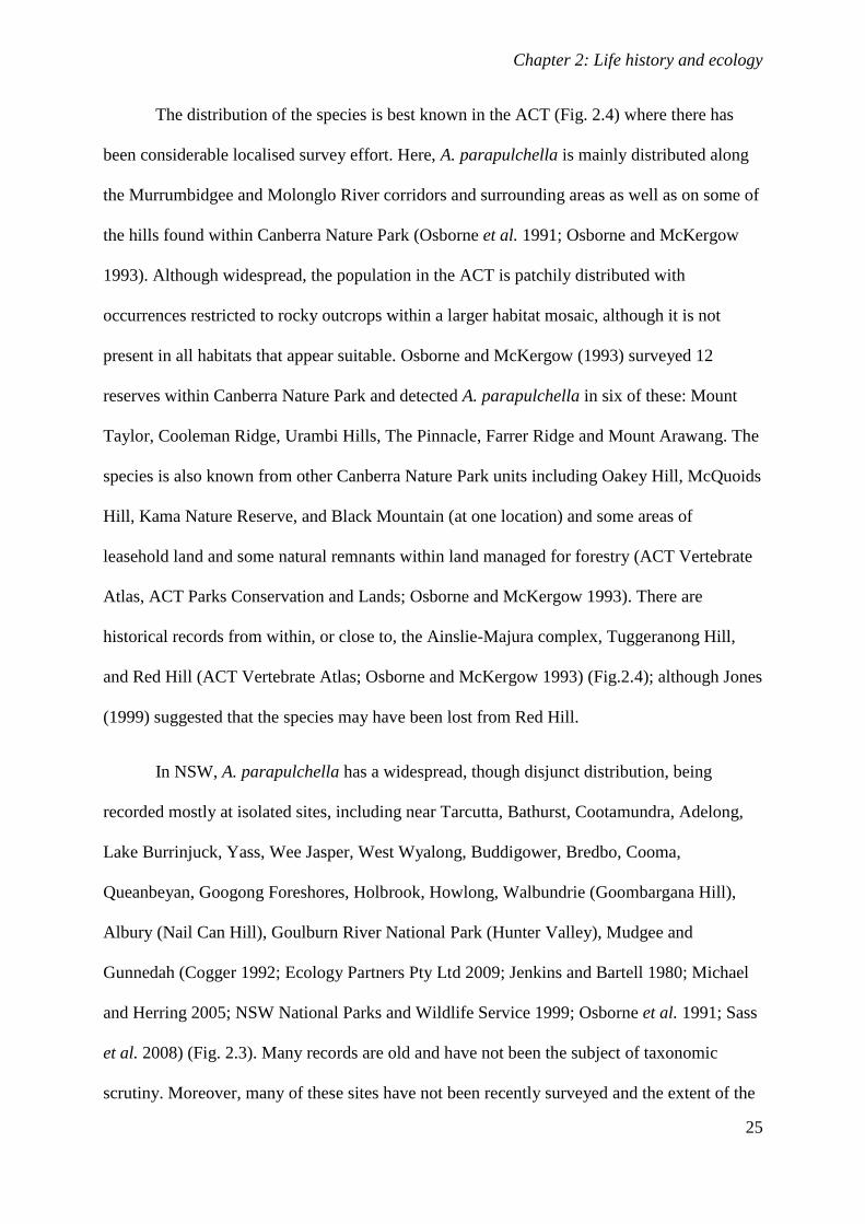
Chapter 2: Life history and ecology
25
The distribution of the species is best known in the ACT (Fig. 2.4) where there has
been considerable localised survey effort. Here, A. parapulchella is mainly distributed along
the Murrumbidgee and Molonglo River corridors and surrounding areas as well as on some of
the hills found within Canberra Nature Park (Osborne et al. 1991; Osborne and McKergow
1993). Although widespread, the population in the ACT is patchily distributed with
occurrences restricted to rocky outcrops within a larger habitat mosaic, although it is not
present in all habitats that appear suitable. Osborne and McKergow (1993) surveyed 12
reserves within Canberra Nature Park and detected A. parapulchella in six of these: Mount
Taylor, Cooleman Ridge, Urambi Hills, The Pinnacle, Farrer Ridge and Mount Arawang. The
species is also known from other Canberra Nature Park units including Oakey Hill, McQuoids
Hill, Kama Nature Reserve, and Black Mountain (at one location) and some areas of
leasehold land and some natural remnants within land managed for forestry (ACT Vertebrate
Atlas, ACT Parks Conservation and Lands; Osborne and McKergow 1993). There are
historical records from within, or close to, the Ainslie-Majura complex, Tuggeranong Hill,
and Red Hill (ACT Vertebrate Atlas; Osborne and McKergow 1993) (Fig.2.4); although Jones
(1999) suggested that the species may have been lost from Red Hill.
In NSW, A. parapulchella has a widespread, though disjunct distribution, being
recorded mostly at isolated sites, including near Tarcutta, Bathurst, Cootamundra, Adelong,
Lake Burrinjuck, Yass, Wee Jasper, West Wyalong, Buddigower, Bredbo, Cooma,
Queanbeyan, Googong Foreshores, Holbrook, Howlong, Walbundrie (Goombargana Hill),
Albury (Nail Can Hill), Goulburn River National Park (Hunter Valley), Mudgee and
Gunnedah (Cogger 1992; Ecology Partners Pty Ltd 2009; Jenkins and Bartell 1980; Michael
and Herring 2005; NSW National Parks and Wildlife Service 1999; Osborne et al. 1991; Sass
et al. 2008) (Fig. 2.3). Many records are old and have not been the subject of taxonomic
scrutiny. Moreover, many of these sites have not been recently surveyed and the extent of the
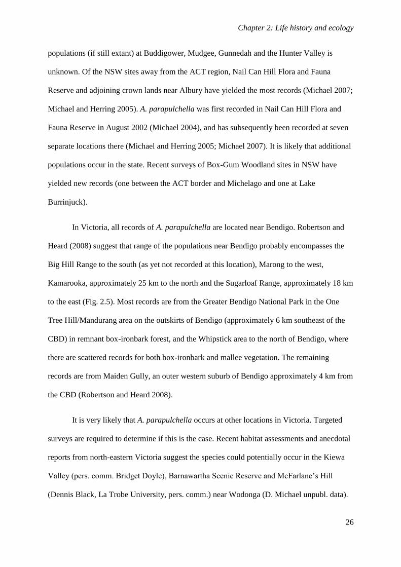
Chapter 2: Life history and ecology
26
populations (if still extant) at Buddigower, Mudgee, Gunnedah and the Hunter Valley is
unknown. Of the NSW sites away from the ACT region, Nail Can Hill Flora and Fauna
Reserve and adjoining crown lands near Albury have yielded the most records (Michael 2007;
Michael and Herring 2005). A. parapulchella was first recorded in Nail Can Hill Flora and
Fauna Reserve in August 2002 (Michael 2004), and has subsequently been recorded at seven
separate locations there (Michael and Herring 2005; Michael 2007). It is likely that additional
populations occur in the state. Recent surveys of Box-Gum Woodland sites in NSW have
yielded new records (one between the ACT border and Michelago and one at Lake
Burrinjuck).
In Victoria, all records of A. parapulchella are located near Bendigo. Robertson and
Heard (2008) suggest that range of the populations near Bendigo probably encompasses the
Big Hill Range to the south (as yet not recorded at this location), Marong to the west,
Kamarooka, approximately 25 km to the north and the Sugarloaf Range, approximately 18 km
to the east (Fig. 2.5). Most records are from the Greater Bendigo National Park in the One
Tree Hill/Mandurang area on the outskirts of Bendigo (approximately 6 km southeast of the
CBD) in remnant box-ironbark forest, and the Whipstick area to the north of Bendigo, where
there are scattered records for both box-ironbark and mallee vegetation. The remaining
records are from Maiden Gully, an outer western suburb of Bendigo approximately 4 km from
the CBD (Robertson and Heard 2008).
It is very likely that A. parapulchella occurs at other locations in Victoria. Targeted
surveys are required to determine if this is the case. Recent habitat assessments and anecdotal
reports from north-eastern Victoria suggest the species could potentially occur in the Kiewa
Valley (pers. comm. Bridget Doyle), Barnawartha Scenic Reserve and McFarlane’s Hill
(Dennis Black, La Trobe University, pers. comm.) near Wodonga (D. Michael unpubl. data).
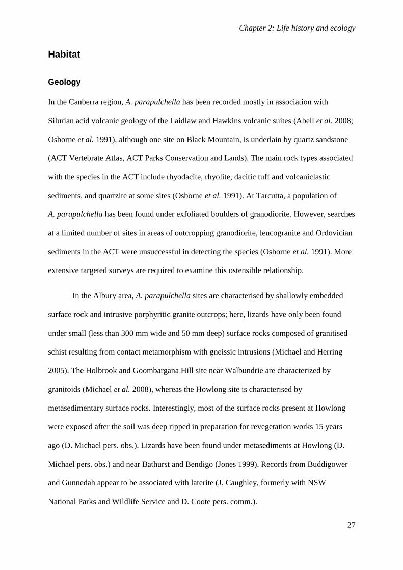
Chapter 2: Life history and ecology
27
Habitat
Geology
In the Canberra region, A. parapulchella has been recorded mostly in association with
Silurian acid volcanic geology of the Laidlaw and Hawkins volcanic suites (Abell et al. 2008;
Osborne et al. 1991), although one site on Black Mountain, is underlain by quartz sandstone
(ACT Vertebrate Atlas, ACT Parks Conservation and Lands). The main rock types associated
with the species in the ACT include rhyodacite, rhyolite, dacitic tuff and volcaniclastic
sediments, and quartzite at some sites (Osborne et al. 1991). At Tarcutta, a population of
A. parapulchella has been found under exfoliated boulders of granodiorite. However, searches
at a limited number of sites in areas of outcropping granodiorite, leucogranite and Ordovician
sediments in the ACT were unsuccessful in detecting the species (Osborne et al. 1991). More
extensive targeted surveys are required to examine this ostensible relationship.
In the Albury area, A. parapulchella sites are characterised by shallowly embedded
surface rock and intrusive porphyritic granite outcrops; here, lizards have only been found
under small (less than 300 mm wide and 50 mm deep) surface rocks composed of granitised
schist resulting from contact metamorphism with gneissic intrusions (Michael and Herring
2005). The Holbrook and Goombargana Hill site near Walbundrie are characterized by
granitoids (Michael et al. 2008), whereas the Howlong site is characterised by
metasedimentary surface rocks. Interestingly, most of the surface rocks present at Howlong
were exposed after the soil was deep ripped in preparation for revegetation works 15 years
ago (D. Michael pers. obs.). Lizards have been found under metasediments at Howlong (D.
Michael pers. obs.) and near Bathurst and Bendigo (Jones 1999). Records from Buddigower
and Gunnedah appear to be associated with laterite (J. Caughley, formerly with NSW
National Parks and Wildlife Service and D. Coote pers. comm.).
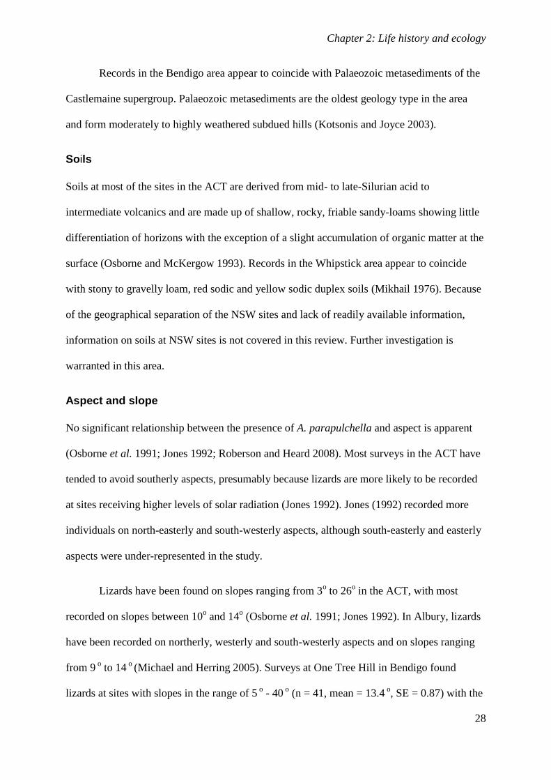
Chapter 2: Life history and ecology
28
Records in the Bendigo area appear to coincide with Palaeozoic metasediments of the
Castlemaine supergroup. Palaeozoic metasediments are the oldest geology type in the area
and form moderately to highly weathered subdued hills (Kotsonis and Joyce 2003).
Soils
Soils at most of the sites in the ACT are derived from mid- to late-Silurian acid to
intermediate volcanics and are made up of shallow, rocky, friable sandy-loams showing little
differentiation of horizons with the exception of a slight accumulation of organic matter at the
surface (Osborne and McKergow 1993). Records in the Whipstick area appear to coincide
with stony to gravelly loam, red sodic and yellow sodic duplex soils (Mikhail 1976). Because
of the geographical separation of the NSW sites and lack of readily available information,
information on soils at NSW sites is not covered in this review. Further investigation is
warranted in this area.
Aspect and slope
No significant relationship between the presence of A. parapulchella and aspect is apparent
(Osborne et al. 1991; Jones 1992; Roberson and Heard 2008). Most surveys in the ACT have
tended to avoid southerly aspects, presumably because lizards are more likely to be recorded
at sites receiving higher levels of solar radiation (Jones 1992). Jones (1992) recorded more
individuals on north-easterly and south-westerly aspects, although south-easterly and easterly
aspects were under-represented in the study.
Lizards have been found on slopes ranging from 3o to 26
o in the ACT, with most
recorded on slopes between 10o and 14
o (Osborne et al. 1991; Jones 1992). In Albury, lizards
have been recorded on northerly, westerly and south-westerly aspects and on slopes ranging
from 9 o to 14
o (Michael and Herring 2005). Surveys at One Tree Hill in Bendigo found
lizards at sites with slopes in the range of 5 o - 40
o (n = 41, mean = 13.4
o, SE = 0.87) with the
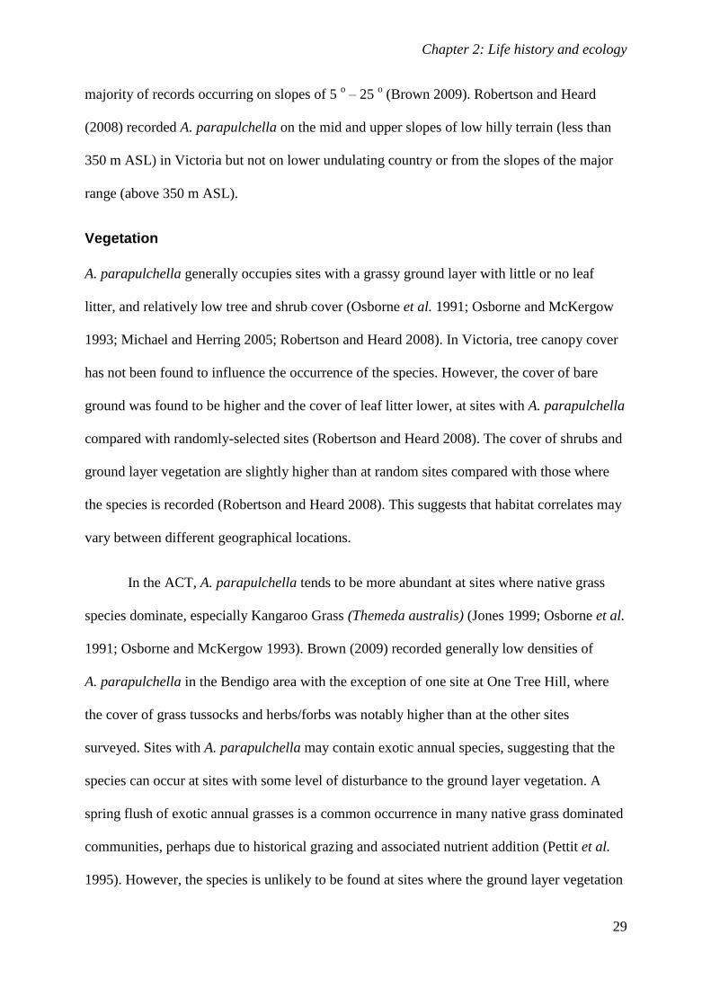
Chapter 2: Life history and ecology
29
majority of records occurring on slopes of 5 o – 25
o (Brown 2009). Robertson and Heard
(2008) recorded A. parapulchella on the mid and upper slopes of low hilly terrain (less than
350 m ASL) in Victoria but not on lower undulating country or from the slopes of the major
range (above 350 m ASL).
Vegetation
A. parapulchella generally occupies sites with a grassy ground layer with little or no leaf
litter, and relatively low tree and shrub cover (Osborne et al. 1991; Osborne and McKergow
1993; Michael and Herring 2005; Robertson and Heard 2008). In Victoria, tree canopy cover
has not been found to influence the occurrence of the species. However, the cover of bare
ground was found to be higher and the cover of leaf litter lower, at sites with A. parapulchella
compared with randomly-selected sites (Robertson and Heard 2008). The cover of shrubs and
ground layer vegetation are slightly higher than at random sites compared with those where
the species is recorded (Robertson and Heard 2008). This suggests that habitat correlates may
vary between different geographical locations.
In the ACT, A. parapulchella tends to be more abundant at sites where native grass
species dominate, especially Kangaroo Grass (Themeda australis) (Jones 1999; Osborne et al.
1991; Osborne and McKergow 1993). Brown (2009) recorded generally low densities of
A. parapulchella in the Bendigo area with the exception of one site at One Tree Hill, where
the cover of grass tussocks and herbs/forbs was notably higher than at the other sites
surveyed. Sites with A. parapulchella may contain exotic annual species, suggesting that the
species can occur at sites with some level of disturbance to the ground layer vegetation. A
spring flush of exotic annual grasses is a common occurrence in many native grass dominated
communities, perhaps due to historical grazing and associated nutrient addition (Pettit et al.
1995). However, the species is unlikely to be found at sites where the ground layer vegetation
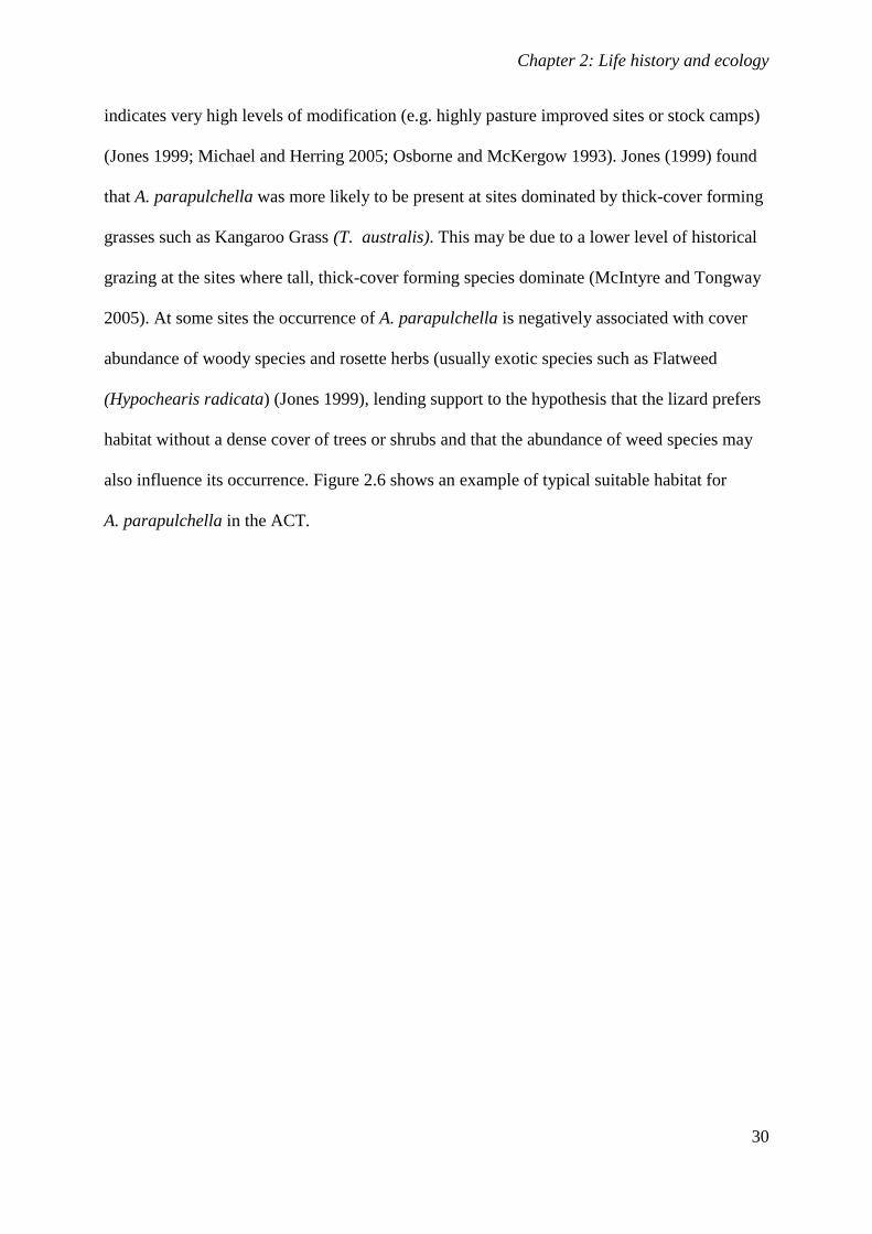
Chapter 2: Life history and ecology
30
indicates very high levels of modification (e.g. highly pasture improved sites or stock camps)
(Jones 1999; Michael and Herring 2005; Osborne and McKergow 1993). Jones (1999) found
that A. parapulchella was more likely to be present at sites dominated by thick-cover forming
grasses such as Kangaroo Grass (T. australis). This may be due to a lower level of historical
grazing at the sites where tall, thick-cover forming species dominate (McIntyre and Tongway
2005). At some sites the occurrence of A. parapulchella is negatively associated with cover
abundance of woody species and rosette herbs (usually exotic species such as Flatweed
(Hypochearis radicata) (Jones 1999), lending support to the hypothesis that the lizard prefers
habitat without a dense cover of trees or shrubs and that the abundance of weed species may
also influence its occurrence. Figure 2.6 shows an example of typical suitable habitat for
A. parapulchella in the ACT.
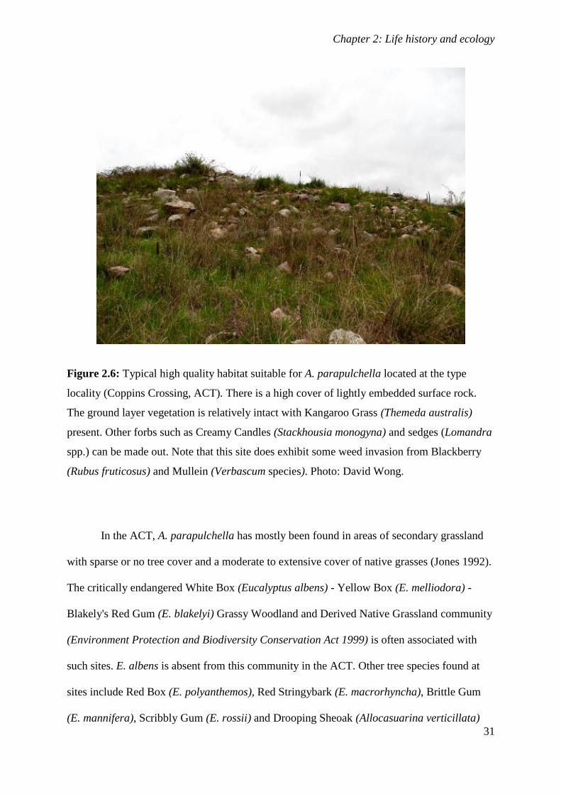
Chapter 2: Life history and ecology
31
Figure 2.6: Typical high quality habitat suitable for A. parapulchella located at the type
locality (Coppins Crossing, ACT). There is a high cover of lightly embedded surface rock.
The ground layer vegetation is relatively intact with Kangaroo Grass (Themeda australis)
present. Other forbs such as Creamy Candles (Stackhousia monogyna) and sedges (Lomandra
spp.) can be made out. Note that this site does exhibit some weed invasion from Blackberry
(Rubus fruticosus) and Mullein (Verbascum species). Photo: David Wong.
In the ACT, A. parapulchella has mostly been found in areas of secondary grassland
with sparse or no tree cover and a moderate to extensive cover of native grasses (Jones 1992).
The critically endangered White Box (Eucalyptus albens) - Yellow Box (E. melliodora) -
Blakely's Red Gum (E. blakelyi) Grassy Woodland and Derived Native Grassland community
(Environment Protection and Biodiversity Conservation Act 1999) is often associated with
such sites. E. albens is absent from this community in the ACT. Other tree species found at
sites include Red Box (E. polyanthemos), Red Stringybark (E. macrorhyncha), Brittle Gum
(E. mannifera), Scribbly Gum (E. rossii) and Drooping Sheoak (Allocasuarina verticillata)
Chapter 2: Life history and ecology
32
(Barrer 1992; Jones 1999; Osborne et al. 1991; Osborne and McKergow 1993).
A. parapulchella has also occasionally been found in Burgan (Kunzea ericoides) shrubland
woodland or open forest (e.g. Black Mountain); usually in more open areas (Barrer 1992;
Osborne and McKergow 1993; D. Wong pers. obs.). Shrub species found at sites occupied by
A. parapulchella may include Burgan (Kunzea ericoides), Blackthorn (Bursaria spinosa
subsp. Lasiophylla), Cassinia spp., Juniper Grevillea (Grevillea juniperina), Urn Heath
(Melichrus urceolatus) and Daphne Heath (Brachyloma daphnoides) (Osborne et al. 1991).
Dominant grass species include Kangaroo Grass (T. australis), Red Grass (Bothriochloa
macra) and Speargrass (Austrostipa scabra).
Discriminant functional analysis revealed the abundance of Squirrel Tail Fescue
(Vulpia bromoides), Wild Oats (Avena fatua), Red Grass (Bothriochloa macra), Delicate
Hairgrass (Aira elegantissima) and Wattle Mat-rush (Lomandra filiformis) to be associated
with A. parapulchella sites (Jones 1999). Sheep’s Burr (Acaena ovina) and Tall Speargrass
(A. bigeniculata) were associated with sites where the species was not recorded. Kangaroo
Grass (T. australis) has also been found to be an important species for A. parapulchella,
especially if it occurs as a dominant species (Osborne et al. 1991; Osborne and McKergow
1993; Jones 1999). The association with the aforementioned exotic species is surprising, but
probably due to the fact that many of the sites that were surveyed were in secondary grassland
that had undergone some level of grazing in the past and exhibited a degree of weed invasion
rather than due to a preference for sites containing those species (Jones 1999).
Chapter 2: Life history and ecology
33
In NSW, vegetation associations appear to be similar to those in the ACT, with
A. parapulchella occurring primarily in grassland, secondary grassland, grassy woodlands
and, occasionally, open forest. The West Wyalong site is an exception as the vegetation there
consists of mallee and broombush and is similar to that found at Whipstick near Bendigo
(Jones 1999).
Sites in the Nail Can Hill Flora and Fauna Reserve in Albury support the endangered White
Box (Eucalyptus albens) - Yellow Box (E. melliodora) - Blakely's Red Gum (E. blakelyi)
Grassy Woodland and Derived Native Grassland community (Environment Protection and
Biodiversity Conservation Act 1999). Where sites are located within woodland, Blakely’s Red
Gum is the dominant species and projective foliage cover is relatively low when compared
with some nearby sites (Michael and Herring 2005). A sparse layer of native shrubs may be
present, with the ground layer usually comprising Kangaroo Grass (T. australis) and other
native grasses and forbs as well as introduced grasses in some areas. At these sites, the lizard
has only been recorded in open areas away from canopy cover (Michael and Herring 2005)
(Fig. 2.7). One individual was recorded in secondary grassland dominated by exotic pasture
grasses and Paterson’s Curse (Echium plantagineum) (Michael 2007).
At the Howlong site, a previously cleared hillside was extensively deep ripped and
revegetated with local species of trees and shrubs [Drooping Sheoak, Acacia spp., Cypress
Pine (Callitris glaucophylla) and White Box (E. albens)] approximately 15 years ago. The
site still supports scattered White Box (E. albens) and Blakely's Red Gum (E. blakelyi) trees
and the ground cover is dominated by Purple Wiregrass (Aristida ramosa), exotic annuals and
forbs (D. Michael, pers. obs.).
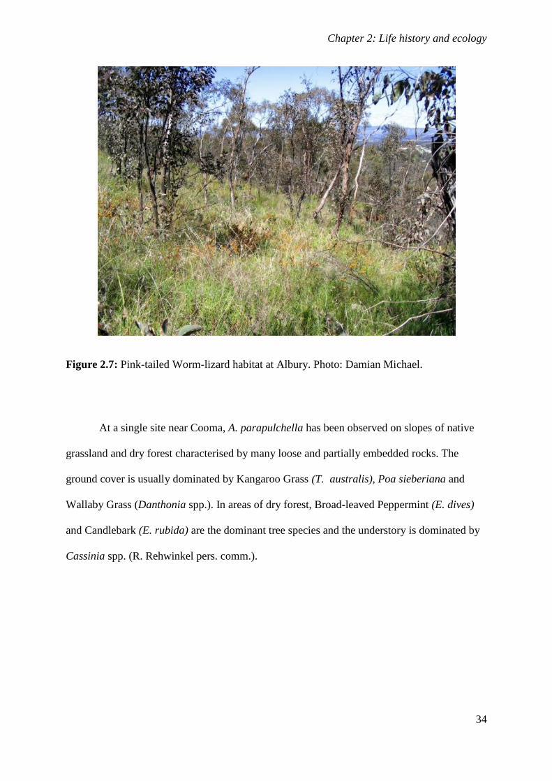
Chapter 2: Life history and ecology
34
Figure 2.7: Pink-tailed Worm-lizard habitat at Albury. Photo: Damian Michael.
At a single site near Cooma, A. parapulchella has been observed on slopes of native
grassland and dry forest characterised by many loose and partially embedded rocks. The
ground cover is usually dominated by Kangaroo Grass (T. australis), Poa sieberiana and
Wallaby Grass (Danthonia spp.). In areas of dry forest, Broad-leaved Peppermint (E. dives)
and Candlebark (E. rubida) are the dominant tree species and the understory is dominated by
Cassinia spp. (R. Rehwinkel pers. comm.).
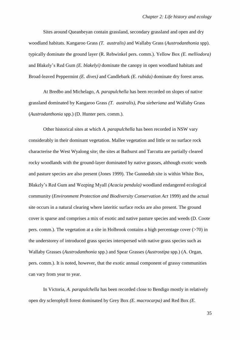
Chapter 2: Life history and ecology
35
Sites around Queanbeyan contain grassland, secondary grassland and open and dry
woodland habitats. Kangaroo Grass (T. australis) and Wallaby Grass (Austrodanthonia spp).
typically dominate the ground layer (R. Rehwinkel pers. comm.). Yellow Box (E. melliodora)
and Blakely’s Red Gum (E. blakelyi) dominate the canopy in open woodland habitats and
Broad-leaved Peppermint (E. dives) and Candlebark (E. rubida) dominate dry forest areas.
At Bredbo and Michelago, A. parapulchella has been recorded on slopes of native
grassland dominated by Kangaroo Grass (T. australis), Poa sieberiana and Wallaby Grass
(Austrodanthonia spp.) (D. Hunter pers. comm.).
Other historical sites at which A. parapulchella has been recorded in NSW vary
considerably in their dominant vegetation. Mallee vegetation and little or no surface rock
characterise the West Wyalong site; the sites at Bathurst and Tarcutta are partially cleared
rocky woodlands with the ground-layer dominated by native grasses, although exotic weeds
and pasture species are also present (Jones 1999). The Gunnedah site is within White Box,
Blakely’s Red Gum and Weeping Myall (Acacia pendula) woodland endangered ecological
community (Environment Protection and Biodiversity Conservation Act 1999) and the actual
site occurs in a natural clearing where lateritic surface rocks are also present. The ground
cover is sparse and comprises a mix of exotic and native pasture species and weeds (D. Coote
pers. comm.). The vegetation at a site in Holbrook contains a high percentage cover (>70) in
the understorey of introduced grass species interspersed with native grass species such as
Wallaby Grasses (Austrodanthonia spp.) and Spear Grasses (Austrostipa spp.) (A. Organ,
pers. comm.). It is noted, however, that the exotic annual component of grassy communities
can vary from year to year.
In Victoria, A. parapulchella has been recorded close to Bendigo mostly in relatively
open dry sclerophyll forest dominated by Grey Box (E. macrocarpa) and Red Box (E.
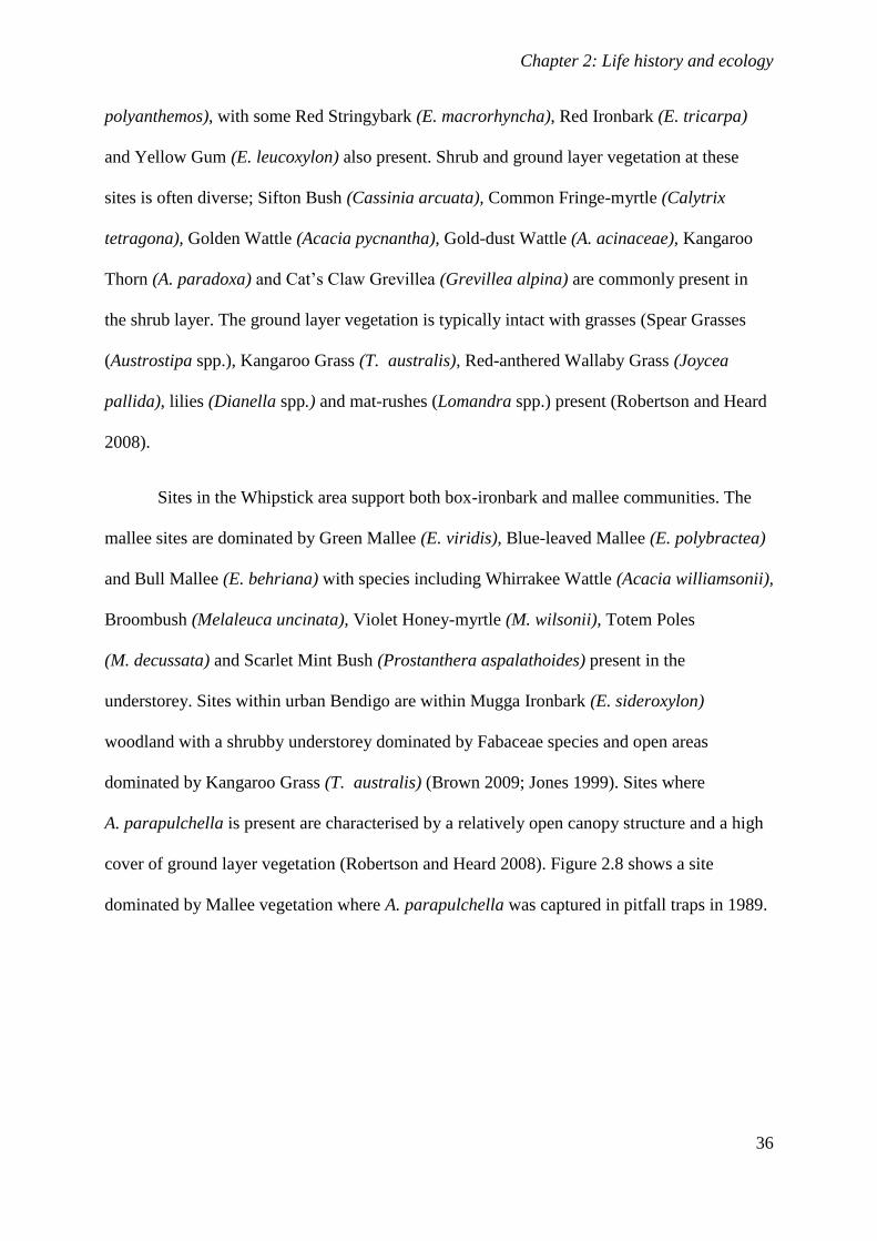
Chapter 2: Life history and ecology
36
polyanthemos), with some Red Stringybark (E. macrorhyncha), Red Ironbark (E. tricarpa)
and Yellow Gum (E. leucoxylon) also present. Shrub and ground layer vegetation at these
sites is often diverse; Sifton Bush (Cassinia arcuata), Common Fringe-myrtle (Calytrix
tetragona), Golden Wattle (Acacia pycnantha), Gold-dust Wattle (A. acinaceae), Kangaroo
Thorn (A. paradoxa) and Cat’s Claw Grevillea (Grevillea alpina) are commonly present in
the shrub layer. The ground layer vegetation is typically intact with grasses (Spear Grasses
(Austrostipa spp.), Kangaroo Grass (T. australis), Red-anthered Wallaby Grass (Joycea
pallida), lilies (Dianella spp.) and mat-rushes (Lomandra spp.) present (Robertson and Heard
2008).
Sites in the Whipstick area support both box-ironbark and mallee communities. The
mallee sites are dominated by Green Mallee (E. viridis), Blue-leaved Mallee (E. polybractea)
and Bull Mallee (E. behriana) with species including Whirrakee Wattle (Acacia williamsonii),
Broombush (Melaleuca uncinata), Violet Honey-myrtle (M. wilsonii), Totem Poles
(M. decussata) and Scarlet Mint Bush (Prostanthera aspalathoides) present in the
understorey. Sites within urban Bendigo are within Mugga Ironbark (E. sideroxylon)
woodland with a shrubby understorey dominated by Fabaceae species and open areas
dominated by Kangaroo Grass (T. australis) (Brown 2009; Jones 1999). Sites where
A. parapulchella is present are characterised by a relatively open canopy structure and a high
cover of ground layer vegetation (Robertson and Heard 2008). Figure 2.8 shows a site
dominated by Mallee vegetation where A. parapulchella was captured in pitfall traps in 1989.
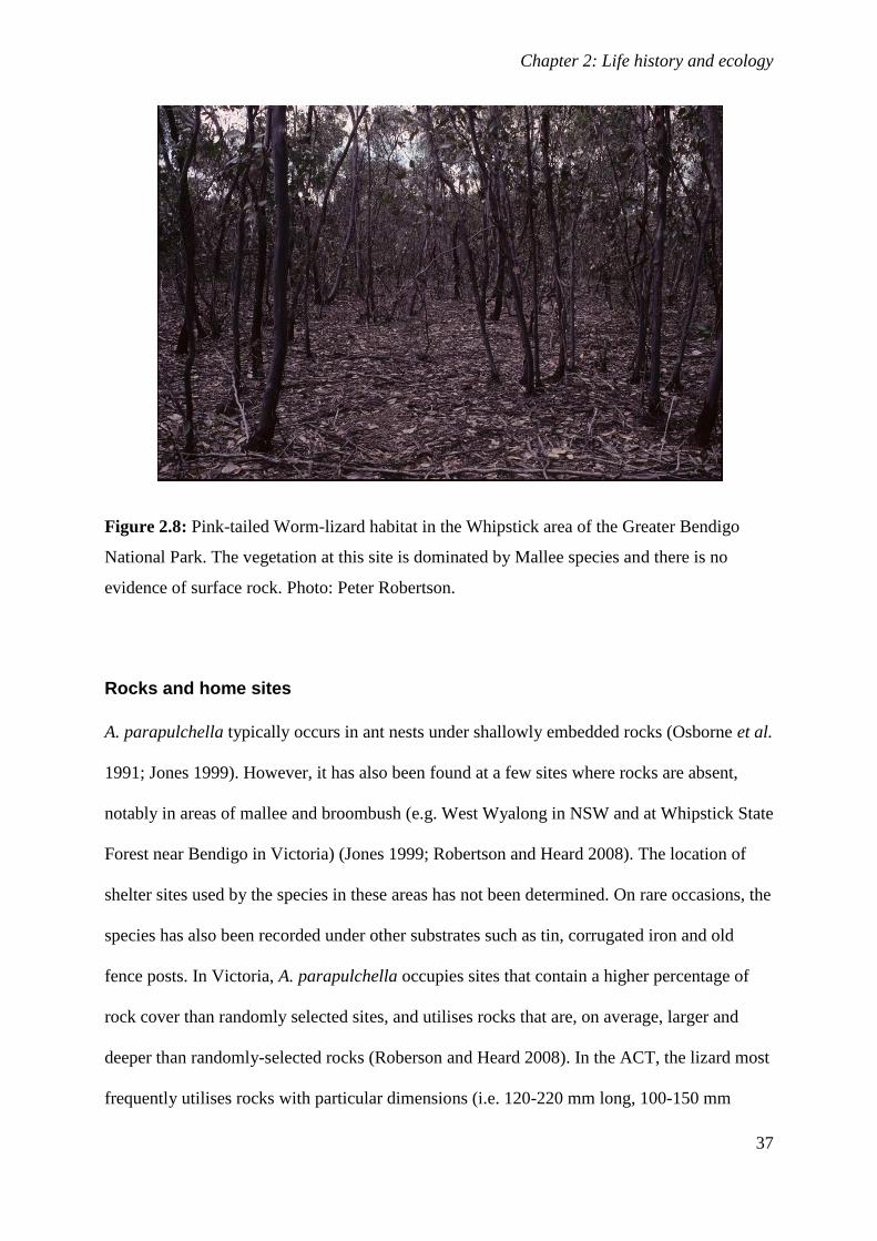
Chapter 2: Life history and ecology
37
Figure 2.8: Pink-tailed Worm-lizard habitat in the Whipstick area of the Greater Bendigo
National Park. The vegetation at this site is dominated by Mallee species and there is no
evidence of surface rock. Photo: Peter Robertson.
Rocks and home sites
A. parapulchella typically occurs in ant nests under shallowly embedded rocks (Osborne et al.
1991; Jones 1999). However, it has also been found at a few sites where rocks are absent,
notably in areas of mallee and broombush (e.g. West Wyalong in NSW and at Whipstick State
Forest near Bendigo in Victoria) (Jones 1999; Robertson and Heard 2008). The location of
shelter sites used by the species in these areas has not been determined. On rare occasions, the
species has also been recorded under other substrates such as tin, corrugated iron and old
fence posts. In Victoria, A. parapulchella occupies sites that contain a higher percentage of
rock cover than randomly selected sites, and utilises rocks that are, on average, larger and
deeper than randomly-selected rocks (Roberson and Heard 2008). In the ACT, the lizard most
frequently utilises rocks with particular dimensions (i.e. 120-220 mm long, 100-150 mm
Chapter 2: Life history and ecology
38
wide, 10-140 mm thick) and is more likely to be found under larger rocks in the winter and
summer months, perhaps owing to the greater insulation and heat retention that such rocks
would afford (Jones 1999). Rock selection also tends to vary with sex in the ACT, with
females more likely to occur under longer and thicker rocks than males (Jones 1999). Rocks
occupied by A. parapulchella are usually located on soil substrate rather than on rock, grass or
litter (Jones 1999; Robertson and Heard 2008; Brown 2009).
Rocks are also an important habitat element for the ants that co-occur with A. parapulchella.
A. parapulchella is a dietary specialist, feeding mainly on the eggs and larvae of small ants
(Jones 1992; Patchell and Shine 1986). Ant galleries are important foraging and shelter sites
for A. parapulchella and provide a thermally stable environment. Figure 2.9 depicts an
A. parapulchella specimen and the ant gallery it was found sheltering in. Sloughed skins are
sometimes found under rocks (Fig. 2.10), and may indicate long-term site fidelity or current
occupancy.
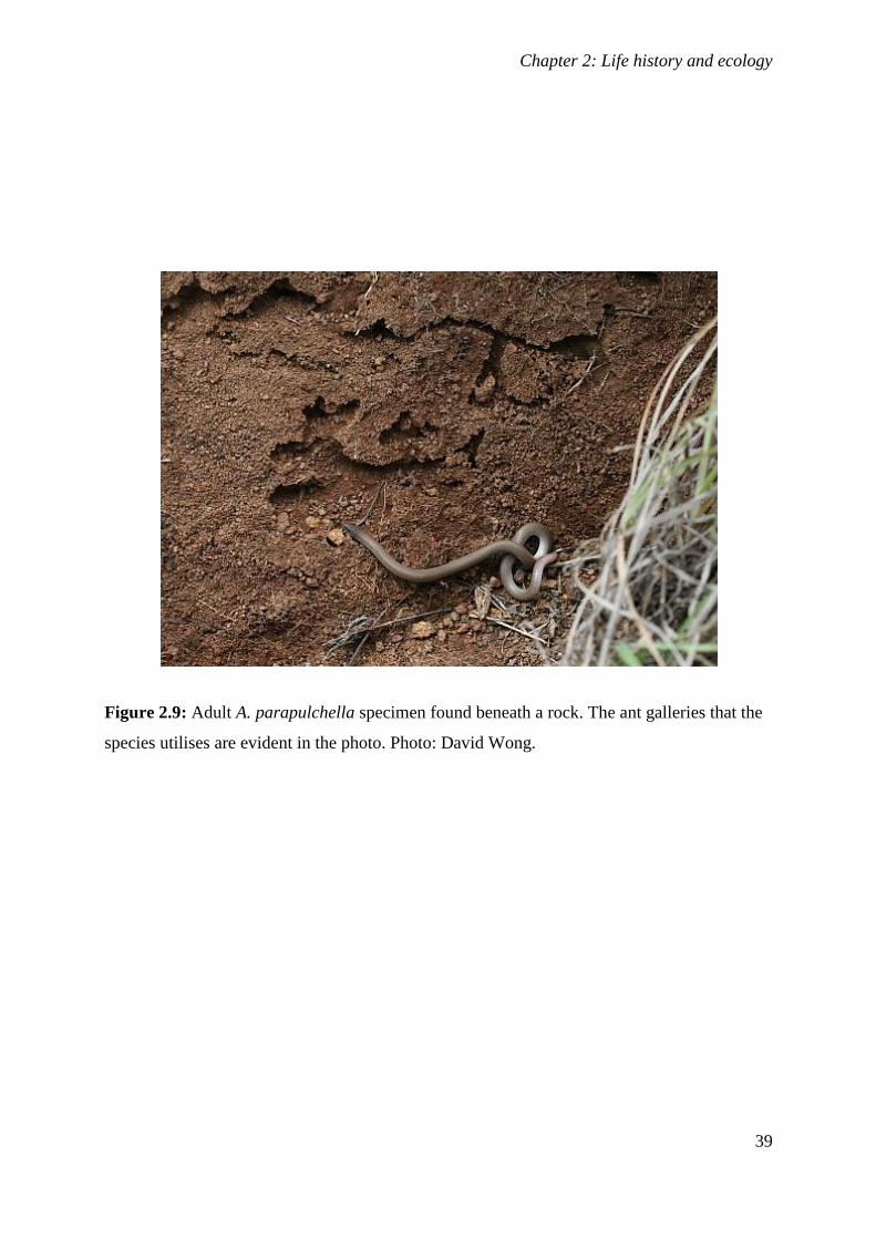
Chapter 2: Life history and ecology
39
Figure 2.9: Adult A. parapulchella specimen found beneath a rock. The ant galleries that the
species utilises are evident in the photo. Photo: David Wong.
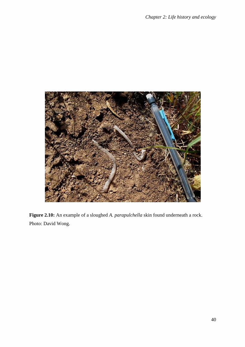
Chapter 2: Life history and ecology
40
Figure 2.10: An example of a sloughed A. parapulchella skin found underneath a rock.
Photo: David Wong.
Chapter 2: Life history and ecology
41
Population attributes
Differences in the size of specimens measured in the ACT appear to be representative of
different annual age classes (Jones 1999) (Table 1). Most specimens in the ACT have a snout-
vent length between 100 mm and 130 mm but have been recorded to a maximum snout-vent
length (SVL) of 150mm (Osborne and McKergow 1993; Jones 1999). Mean weight and SVL
of adults in the ACT and Victoria (Jones 1999; Robertson and Heard 2008; Brown 2009;
Wong 2008 and 2009 unpublished data) differ substantially (Table 2). Jones (1999) recorded
weights ranging between 0.15 g and 2.6 g, whereas individuals in Bendigo weighed between
0.1 g and 4.0 g (Robertson and Heard 2008). Comparing mean SVL and weight for adults in
the ACT (Wong and Osborne 2008; 2009, unpublished data) with those in Victoria
(Robertson and Heard 2008; Brown 2009) reveals Victorian males and females to be
significantly longer and heavier than conspecifics in the ACT (Table 2).
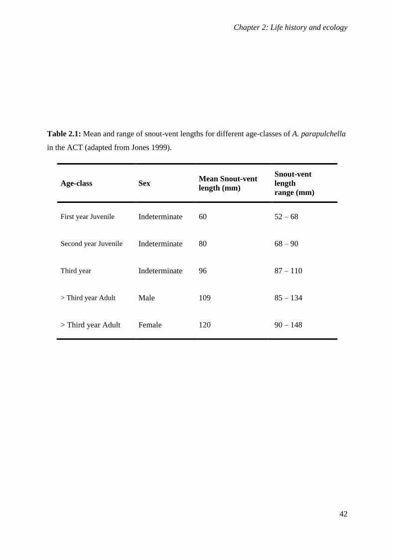
Chapter 2: Life history and ecology
42
Table 2.1: Mean and range of snout-vent lengths for different age-classes of A. parapulchella
in the ACT (adapted from Jones 1999).
Age-class Sex Mean Snout-vent
length (mm)
Snout-vent
length
range (mm)
First year Juvenile Indeterminate 60 52 – 68
Second year Juvenile Indeterminate 80 68 – 90
Third year Indeterminate 96 87 – 110
> Third year Adult Male 109 85 – 134
> Third year Adult Female 120 90 – 148
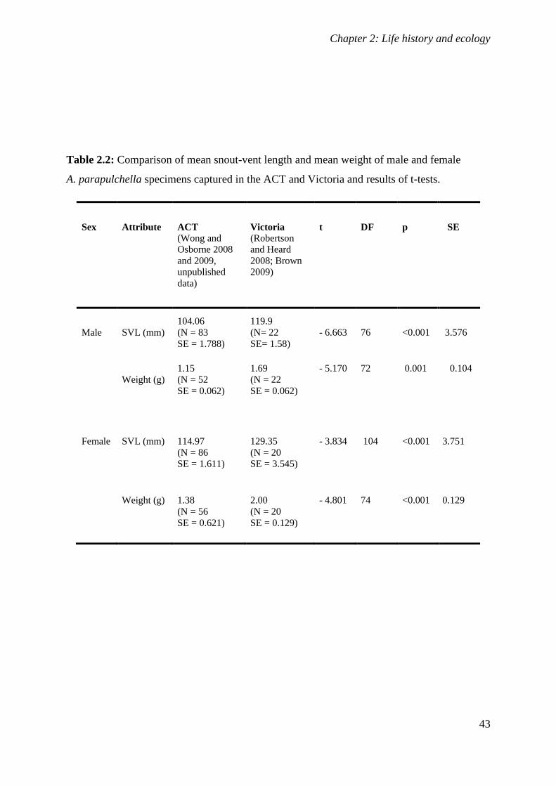
Chapter 2: Life history and ecology
43
Table 2.2: Comparison of mean snout-vent length and mean weight of male and female
A. parapulchella specimens captured in the ACT and Victoria and results of t-tests.
Sex
Attribute
ACT
(Wong and
Osborne 2008
and 2009,
unpublished
data)
Victoria
(Robertson
and Heard
2008; Brown
2009)
t
DF
p
SE
Male
SVL (mm)
104.06
(N = 83
SE = 1.788)
119.9
(N= 22
SE= 1.58)
- 6.663
76
<0.001
3.576
Weight (g)
1.15
(N = 52
SE = 0.062)
1.69
(N = 22
SE = 0.062)
- 5.170 72 0.001 0.104
Female SVL (mm)
114.97
(N = 86
SE = 1.611)
129.35
(N = 20
SE = 3.545)
- 3.834 104 <0.001 3.751
Weight (g) 1.38
(N = 56
SE = 0.621)
2.00
(N = 20
SE = 0.129)
- 4.801 74 <0.001 0.129
Chapter 2: Life history and ecology
44
A. parapulchella is reported to have an even sex-ratio (Jones 1999, Robertson and
Heard 2008) and displays sexual dimorphism, with females being longer and heavier than
males (Jones 1999; Robertson and Heard 2008), probably due to the demands of carrying
eggs (Kluge 1974). Ghiselin (1974) suggested that, in species where females are sedentary
and sparse, selection may favour relatively smaller males owing to the lower metabolic
demands of smaller individuals. Tail length is not significantly different between males and
females (Jones 1999; Robertson and Heard 2008; Brown 2009).
The estimation of population size through the use of traditional mark-recapture
methods presents difficulties in fossorial reptiles (Henle 1989). A mark-recapture study
undertaken at Mount Taylor yielded low recapture rates (6%), yet provided a population
estimate of 312 individuals (with upper and lower confidence limits of 599 and 145) (Jones
1999). A 1992 survey of a dam site on the Lower Molonglo River yielded a population
estimate of 37 individuals after 3000 rocks were turned (Barrer 1992, cited in Jones 1999).
This was substantially lower than the population estimate of 157 based on 151 individuals
from 40 000 rocks subsequently turned at the same site during the complete removal of all
stones (Jones 1999). Such disparities underscore the risk of relying on single sampling events.
In the Albury area, the maximum number of individuals recorded during a single
survey period was 58 individuals within an area of 3.6 ha at one location (along a ridge) and
12 individuals within an area of 1 ha at a second location (Michael and Herring 2005).
A comparison of relative density figures recorded in Victoria (N = 15) and the ACT (N = 57)
(Jones 1992; Jones 1999; Robertson and Heard 2008; Brown 1999; Wong 2008 - 2009,
unpublished data) reveals mean relative density of A. parapulchella estimated at sites where
more than 250 rocks were turned to be higher in the ACT (Mean = 5.7 specimens per 1000
stones; N = 57; SD = 3.32) than Bendigo (Mean = 3.5 specimens per 1000 stones; N = 15;
Chapter 2: Life history and ecology
45
SD = 3.44). A t-test performed on log-transformed data revealed a highly significant
difference between lizard density at the two locations (t = 3.357; df = 70; p = 0.001).
The differences in density and body size observed in the Victorian and ACT
populations are intriguing and warrant further attention. Differences in density may be due to
a range of factors. The role of shading in determining thermal conditions is likely to be an
important factor and has been found to be important for other reptile species (Michael et al.
2008). Unravelling the causes of differences in body size can be difficult as there may be a
number of interacting biophysical, physiological and population level factors involved
(Dunham et al. 1989). However, factors influencing body size at the two locations may
include altitude, density of lizards, availability of cover, food and shelter, site availability and
the influence of canopy cover on the thermal environment or predation pressure (Ballinger
1979; Dunham et al. 1989).
Reproduction
Co-occurrence of individuals beneath stones has been observed in September (G. Kay pers.
obs.) and October (Jones 1999) and gravid specimens have been observed in late November
and December (Kluge 1974; Jones 1999; Robertson and Heard 2008). Jones (1999) inferred,
from data on the smallest individuals observed to be sharing a rock with an individual of the
opposite sex, that sexual maturity is probably reached in males at a snout-vent length (SVL)
of at least 102 mm (in the third year of life) and in females with an SVL of at least 118 mm
(around the fourth year of life). The relatively late maturation in the species suggests that it is
relatively long-lived (Jones 1999). While there is no information on oviposition in
A. parapulchella, it is likely that ant, and perhaps termite, nests are used. This has been
documented for other reptiles (De Lisle 1996; Riley et al. 1985; Velásquez-Múnera et al.
Chapter 2: Life history and ecology
46
2008). There are no specific records of hatching dates, though hatching is likely to take place
in mid- to late summer.
Activity patterns and movement
A. parapulchella mostly lives under rocks and occupies inhabited or uninhabited ant nests
(Jones 1999; Osborne et al. 1991). Observations of the lizard’s activity patterns in the field
are limited, due to its cryptic and fossorial nature. Laboratory observations reveal that the
lizard is active during the day but not at night time, suggesting a diurnal activity pattern. As
well as eating, drinking and moving through grass tussocks in a tank, lizards were observed to
sometimes spend days buried under the sandy substrate. Dampening the substrate tended to
increase movement around the tank (Jones 1992). In the field, A. parapulchella may be more
readily detected under rocks shortly after rainfall when there is some moisture in the soil
profile (Osborne et al. 1991). This may indicate that the lizards move up to the surface from
deeper in the ant burrows during these times in particular.
Above-ground daytime activity has been documented for A. parapulchella in the field.
Such diurnal activity includes basking on a rock or in a tussock close to a rock, moving
rapidly through grass and bare ground and traversing a walking track during the warmer
spring months (Barrer 1992; Jones 1992; Osborne and McKergow 1993; P. Robertson pers.
obs.). Lizards have also been collected on roadsides and in urban areas (R. Bennett pers.
comm.). Rauhala (1993) captured eleven A. parapulchella in pitfall traps at three sites in the
Stony Creek Nature Reserve (located within the Murrumbidgee River Corridor in the ACT)
during pitfall trapping undertaken between November and December 1992 and in March
1993. One of these was located in atypical habitat – tall open scrub (Kunzea ericoides and
Leptospermum brevipes) with very little rock or grass cover.
Chapter 2: Life history and ecology
47
In the ACT, Jones (1999) conducted pitfall trapping (16,536 trap nights) at a single
site in rocky habitat occupied by A. parapulchella and adjacent non-rocky habitat, between
October 1993 and May 1994. Only five specimens of A. parapulchella (2% of total captures)
were recorded (in October and November) during this study, all in rocky habitat. Robertson
and Edwards (1994) observed similar seasonality of movement for the congeneric A. aurita
with most specimens being trapped in late October, aligned with the mating period. Jones
(1999) suggests that the slightly earlier timing of movement for A. aurita, compared with
A. parapulchella may be related to climatic differences.
A recent survey of eleven sites burnt in the 2003 bushfires in the Stromlo Forest area
in the ACT (6 sites in former pine plantation; 5 in remnant native woodland or grassland)
yielded A. parapulchella at two sites previously covered by a mature Monterey Pine Pinus
radiata plantation. Some specimens were at least 30 m from possible source populations (i.e.
rocky habitat areas with remnant native vegetation) and an unexpectedly high density of
lizards (6.9 lizards per 1000 rocks turned) was found at one site that had been planted with
Monterey Pines eight years prior to the fires (D. Wong and W. Osborne, unpublished data).
This finding suggests that the species is able to move across the landscape and occupy new
areas to some extent, though the long-term viability of such occupation is not known.
In the ACT, most specimens have been found in spring. Individuals have been found
under rocks during the autumn and winter; however, detection is unreliable when compared
with spring detection and may be dependent on recent rainfall events. Similarly, in the Albury
region, with the exception of one record, A. parapulchella has only ever been recorded
beneath surface rocks or in funnel traps, between late August and mid-November. The one
exception was a juvenile recorded beneath a small surface rock in early May 2009
(D. Michael pers. obs.).
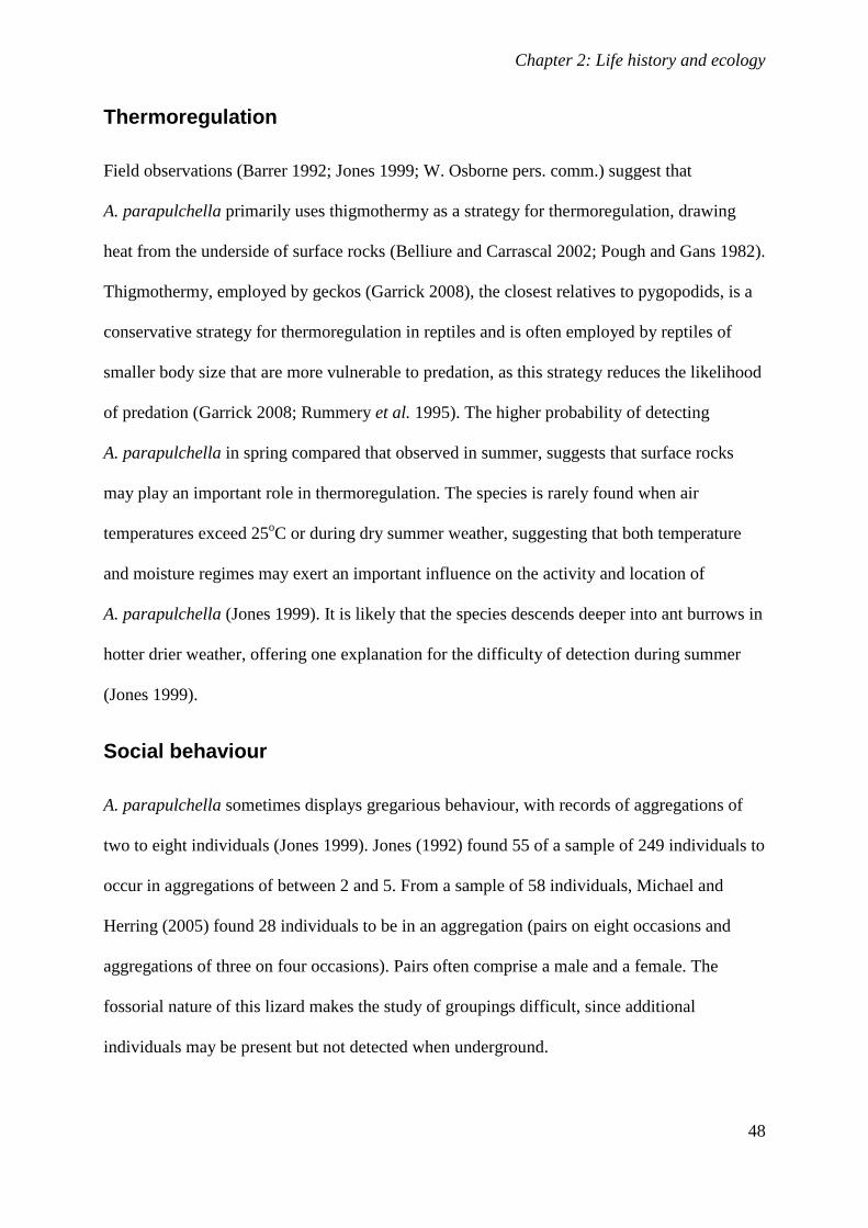
Chapter 2: Life history and ecology
48
Thermoregulation
Field observations (Barrer 1992; Jones 1999; W. Osborne pers. comm.) suggest that
A. parapulchella primarily uses thigmothermy as a strategy for thermoregulation, drawing
heat from the underside of surface rocks (Belliure and Carrascal 2002; Pough and Gans 1982).
Thigmothermy, employed by geckos (Garrick 2008), the closest relatives to pygopodids, is a
conservative strategy for thermoregulation in reptiles and is often employed by reptiles of
smaller body size that are more vulnerable to predation, as this strategy reduces the likelihood
of predation (Garrick 2008; Rummery et al. 1995). The higher probability of detecting
A. parapulchella in spring compared that observed in summer, suggests that surface rocks
may play an important role in thermoregulation. The species is rarely found when air
temperatures exceed 25oC or during dry summer weather, suggesting that both temperature
and moisture regimes may exert an important influence on the activity and location of
A. parapulchella (Jones 1999). It is likely that the species descends deeper into ant burrows in
hotter drier weather, offering one explanation for the difficulty of detection during summer
(Jones 1999).
Social behaviour
A. parapulchella sometimes displays gregarious behaviour, with records of aggregations of
two to eight individuals (Jones 1999). Jones (1992) found 55 of a sample of 249 individuals to
occur in aggregations of between 2 and 5. From a sample of 58 individuals, Michael and
Herring (2005) found 28 individuals to be in an aggregation (pairs on eight occasions and
aggregations of three on four occasions). Pairs often comprise a male and a female. The
fossorial nature of this lizard makes the study of groupings difficult, since additional
individuals may be present but not detected when underground.
Chapter 2: Life history and ecology
49
Relationship with ants
A. parapulchella has been found in association with 15 species of ants (representing 4 to 5
sub-families) and one termite species (Jones 1999). In one study, 75% of A. parapulchella
captures were recorded under rocks also occupied by ants, whilst 90% of lizards captured
were found under rocks where burrows with multiple entrances (characteristic of ant burrows)
were present (Jones 1999). This supports findings by Osborne et al. (1991), who found 79%
of specimens cohabiting with ants and 93% of specimens (N = 46) to be associated with small
burrows. Brown (2009) reported ants beneath only 13% of rocks A. parapulchella were
sheltering beneath near Bendigo, although Robertson and Heard (2008) reported around two-
thirds of rocks had ants or ant burrows associated in the Bendigo area. The differences
observed could be related to the variable nature of ant activity at the surface. The findings of
Jones (1999) suggest that the presence of ants at the surface is affected by season, with
significantly less A. parapulchella found cohabiting with ants in November compared with
the months of March, September and October.
Fifty-three percent of specimens recorded by Jones (1999) co-occurred with one
species of ant, the Tyrant Ant Iridomyrmex rufoniger. This small species aggressively defends
its nests when disturbed by intruders (Jones 1999; Robinson 1996). Analysis by Jones (1999)
using Ivlev’s electivity index (Ivlev 1961) revealed that A. parapulchella preferentially
selected home sites also occupied by I. rufoniger. Electivity analyses of ant sub-families and
functional groups also revealed A. parapulchella to select home sites occupied by species
from the Dolichoderinae sub-family and the Dominant Dolichoderinae functional group.
The mechanism employed by A. parapulchella for avoidance of attack by ants is not
known, although Jones (1999) speculated that it might be related to the lizard’s behaviour or
to chemical signals.
Chapter 2: Life history and ecology
50
Diet
There have been a number of investigations into the diet of pygopodids (e.g. Patchell and
Shine 1986; Webb and Shine 1994). Webb and Shine (1994) found that Aprasia spp. almost
exclusively consumed ant brood, drawing attention to the dietary and morphological
convergence between Aprasia and typhlopid snakes. Jenkins and Bartell (1980), through the
examination of the gut contents of five specimens of A. parapulchella, concluded that small
ants of the genus Iridomyrmex were the most common food item. In a more extensive study
using scanning electron microscopy to examine 163 faecal pellets obtained from
A. parapulchella in the ACT, Jones (1999) found the diet to comprise at least eleven species
of ants and two species of termite. Of the ants, I. rufoniger was by far the most frequently
consumed species, with Pheidole spp., Paratrechina spp. and Rhytidoponera metallica often
appearing in the diet. Adult workers of species consumed by A. parapulchella ranged in size
(1.5 - 4.5 mm long) and more than half of the time were revealed to be co-habiting with
A. parapulchella. For I. rufoniger, this relationship was especially strong, with 77% of
A. parapulchella cohabiting with I. rufoniger found to have consumed the species (Jones
1999). The fact that ant prey taxa were not always the same as those taxa co-habiting with
A. parapulchella suggests that the lizard forages beyond its immediate environment. A recent
study of the diet of the Mallee Worm-lizard (A. aurita) and the Pink-nosed Worm-lizard (A.
inaurita) in north-western Victoria (Wainer et al. in prep.) has revealed similar dietary habits
in these species to those observed in A. parapulchella. A. aurita and A. inaurita consumed
nine and five species of ants respectively. There was significant overlap in the ant species
consumed and a total of only 11 species of ants was recorded in all the scat samples collected
from the two lizard taxa, whilst pitfall trapping in the area has recorded a total of 59 species in
two sampling years indicating that the species are dietary specialists. The ant species
consumed were of similar size to those consumed by A. parapulchella (1.5–3.0 mm) and
Chapter 2: Life history and ecology
51
I. rufoniger was commonly consumed. The authors also observed that the ant taxa consumed
were relatively innocuous species. The species co-occurring with A. parapulchella are similar
in this respect (J. Wainer, DPI Victoria, pers. comm.).
Jones (1999) found that A. parapulchella preferred ant eggs and larvae to adult ants as
food, with eggs being preferred over larvae when they were given access to both in captive
experiments. Adult ants are only occasionally ingested and this is thought to be due to
accidental ingestion of workers tending the brood. This strategy appears to take advantage of
a highly nutritious spatially clumped food source. The only non-ant material discovered in
lizard scats by Jones (1992) was fungal mycelium, thought to be from a group which exists
internally in invertebrates (K. Thomas, University of Canberra, pers. comm.). The findings of
Wainer et al. (in prep.) indicate similar preferences for brood over adults in A. aurita and A.
inaurita.
Tail loss and predation
The pink-coloured tail of A. parapulchella most likely has a role in reducing predation by
drawing the attention of predators away from the head and body (Rankin 1976). Therefore,
tail-loss may not be a good indicator of predation pressure but rather may indicate escape
efficiency or predator inefficiency (Jaksic and Greene 1984; Medel et al. 1988). In the ACT
tail-loss rates in A. parapulchella vary between sites, from 21% to 55% (Osborne and
McKergow 1993; Jones 1999). Jones (1999) suggests that the relatively high level of tail loss
observed at some sites may reflect an ageing population at those sites, with older individuals
more likely to have been exposed to unsuccessful predation attempts (Schoener 1979; Tinkle
and Ballinger 1972). However, it is also possible that predation pressure was higher at those
sites. No significant sex differences in overall tail loss were reported by Jones (1999).
Chapter 2: Life history and ecology
52
Research directions
There is still much to learn about A. parapulchella. The cryptic behaviour of the species has
made it difficult for researchers to address some aspects of its ecology – particularly relating
to breeding biology and thermoregulation (Jones 1999). Further information is required with
respect to oviposition sites, local movements between rock outcrops, social behaviour and
details of the relationship between lizards and ants. Disturbance is thought to be an important
correlate in relation to occurrence of the species in agricultural landscapes but the exact
mechanisms involved are poorly understood. We also need to increase our knowledge of the
species’ distribution and habitat requirements. This will require further targeted field surveys,
particularly in New South Wales and Victoria. In particular, the extent of the apparent
extreme disjunction of the key populations should be examined along with the causes of this.
Currently we do not know to what extent the dominant processes influencing the distribution
are biogeographical or as a result of disturbance or some combination of the two. The larger
body size of individuals collected near Bendigo, when compared to Albury and Canberra is of
interest and may reflect underlying genetic differences. Therefore, surveys should be
accompanied by genetic studies that address evidence for historical dispersal and considers
the effects of fragmentation. Genetic analysis is likely to provide the clearest insights at a
range of scales, providing estimates of dispersal capability and connectivity and the influence
of major barriers such as roads, urban areas, rivers and agricultural landscapes. This
information is essential for informed conservation planning in relation to A. parapulchella.
Conclusion
The existing information on A. parapulchella suggests that it is a habitat and dietary specialist
which has a preference for native grassy areas with rocky cover and a close association with a
number of species of small ants. However, there are some data and observations that suggest
Chapter 2: Life history and ecology
53
that the species also occurs in what could be considered atypical habitat in some locations.
The possibility of spatial variation in habitat preferences, therefore, warrants further
examination. There is evidence to suggest that agricultural disturbance to key habitat and
ecological features is a potential threat to the species. However, more information is required
on the response of the species to disturbance. In addition, determining the extent to which
biogeographical and disturbance factors are likely to have led to the current distribution is an
area of considerable interest. The research on this species to date forms a good foundation for
further exploration of aspects of the species including the ecology and behaviour of the
species as well as the likely biogeographical and environmental factors that have influenced
its current distribution.
Acknowledgements
We thank the following people for providing useful information relating to the species: David
Hunter, Rainer Rehwinkel and David Coote (Department of Environment Climate Change
and Water NSW); Marjo Rauhala, Darren Roso and Peter Beutel (Parks Conservation and
Lands, ACT); John Wainer (Department of Primary Industries, Victoria); Dennis Black (La
Trobe University); Theresa Knopp (Institute for Applied Ecology, University of Canberra);
Aaron Organ (Ecology Partners Pty Ltd); Ross Bennett, Ken Thomas, and Bridget Doyle. Arn
Tolsma (Arthur Rylah Institute for Environmental Research, Department of Sustainability and
the Environment, Victoria) and Felicity Grant (Parks Conservation and Lands, ACT) kindly
helped in the preparation and provision of GIS data for maps and Maria Boyle (University of
Canberra) provided statistical advice. Finally, we thank Percy Wong, Sonya Duus and Ingrid
Stirnemann, Steven Sass and one anonymous reviewer for useful comments on the
manuscript.

54
Chapter 3: Correlates of occurrence
55
3. Clarifying environmental correlates of occurrence for
Aprasia parapulchella using MaxEnt
Abstract
Species distribution models are commonly used to make spatially-explicit predictions
about where a species is likely to occur. However, these methods may also provide
useful information about the relationship between environmental variables and species
occurrence. I used MaxEnt to model the occurrence of the Pink-tailed Worm-lizard
Aprasia parapulchella (Pygopodidae) in the Australian Capital Territory. I assessed the
influence of the environmental variables in the model and the response curves and plots
derived by MaxEnt. The results indicate that, at the regional scale, surficial geology and
soil type contributed most to the model, followed by slope, temperature, rainfall and
agricultural modification. The model outputs helped to confirm, as well as add to, the
current understanding of the response of A. parapulchella to environmental variables.
The modelling revealed a new association with a Devonian-age geological unit.
Relationships between temperature and rainfall variables and the occurrence of
A. parapulchella and temperature are also described. This is the first time that the
distribution of A. parapulchella has been modelled at this spatial scale (approximately
50km x 50km study area). The use, within a species distribution model, of a remotely
sensed classification that discriminates between C3 and C4 species of grass in order to
characterise agricultural modification is also novel. This approach could be used for
other species in order to add to the knowledge of species habitat requirements and the
factors influencing distribution. The results of such modelling exercises are likely to be
Chapter 3: Correlates of occurrence
56
useful for managers and conservation planners, as this is the scale at which conservation
management often operates.
Introduction
Species distribution models (SDMs) are increasingly popular tools for addressing a
range of problems in ecology. The applications may range from predicting potential
habitat of individual species to predicting the impact of climate change or the risk of
weed invasion (for a list of applications see Guisan and Thuiller 2005 and Elith et al.
2011). Broadly speaking, SDMs are applied in order to understand the environmental
drivers of occurrence of a species, or groups of species, or to predict their occurrence in
the landscape (Elith and Leathwick 2009).
Improving our understanding of factors that influence the occurrence of species
is especially important with respect to threatened species because this information may
inform management of known populations and lead to improved conservation outcomes
(e.g. reservation or protection of suitable habitat). SDM applications offer the advantage
of providing information on environmental drivers of distribution as well as spatially-
explicit predictions in order to inform conservation planning.
A systematic survey is often not available for species of interest (Elith et al.
2011). In such situations, presence-only techniques are used. MaxEnt (Phillips et al.
2006; Phillips and Dudík 2008) is a commonly used SDM package as it is one of the
best performing presence-only packages available (Elith et al. 2006). It has been used
very effectively to determine environmental features that correlate with the occurrence
of individual species of wildlife. Monterroso et al. (2009) found that European Rabbit
(Oryctolagus cuniculus) abundance and limited human disturbance were the best
Chapter 3: Correlates of occurrence
57
predictors of European Wildcat (Felis silvestris) in Portugal. It has also been used
effectively in order to characterise the environmental factors influencing co-occurrence
and distribution of three species of viper in Spain (Martínez-Freiría et al. 2008).
MaxEnt has also been used effectively to predict areas of occurrence of a number of
species of reptiles (Gadsden et al. 2012; Houniet et al. 2009; Pawar et al. 2007; Pearson
et al. 2007; Raxworthy et al. 2003).
The Pink-tailed Worm-lizard Aprasia parapulchella (Pygopodidae) Kluge is a
threatened species of legless lizard (Pygopididae) that occurs in south-eastern Australia
(Wong et al. 2011). It is a habitat specialist that relies on native grass cover, lightly
embedded rocks and a number of species of ants that provide its prey (Jones 1999;
Osborne et al. 1991). Previous studies (Jones 1992; Jones 1999; Osborne et al. 1991;
Osborne and McKergow 1993) have identified a number of habitat and environmental
correlates of occurrence for A. parapulchella. The species has been associated with
Silurian-age volcanic geology and the sandy-loam soils derived from this parent
material (Osborne et al. 1991; Osborne and McKergow 1993; Wong et al. 2011).
Specimens have been recorded on slopes of between 3° and 26° with most of the
specimens occurring on slopes between 10° and 14° and at sites experiencing higher
levels of solar radiation (Jones 1992; Osborne et al. 1991). In the Australian Capital
Territory (ACT), the occurrence of A. parapulchella has been associated with sites with
a ground layer dominated by native grasses (particularly Themeda australis) and a
relatively low cover of over-storey vegetation (Jones 1999; Osborne et al. 1991;
Osborne and McKergow 1993). The availability of this detailed information and habitat
requirements provides an ideal basis for applying SDM techniques such as MaxEnt to
further our knowledge about the correlates of occurrence for species such as
Chapter 3: Correlates of occurrence
58
A. parapulchella. Whilst the distribution of the species has been used to model
predicted occurrence of the species across its range (Brown 2009), no modelling has
been done at finer spatial scales.
In this paper I report on a fine spatial-scale (study extent approximately 50km x
50km; grain size = 25m) MaxEnt model that I constructed for A. parapulchella for the
ACT. I use the model to test our understanding of the key environmental correlates
relating to the species occurrence. It is anticipated that the results of this study will
assist conservation planning and management for A. parapulchella by clarifying and
refining knowledge about environmental correlates of occurrence as well as identifying
important regional areas for conservation. They may also identify new areas that
warrant investigation as possible sites occupied by the species.
Methods
Study Area
This study focussed on an approximately 50km x 50km area in the Australian Capital
Territory (ACT) and adjacent land in New South Wales (an area located in south-
eastern Australia between the latitudes of 35 o
1’ 11”S and 35o 28’ 38” S and longitudes
of 147o 19’ 0” E and 147
o 40’ 12” E). This area encompasses most of the known records
of A. parapulchella in the ACT area (Fig. 3.1).
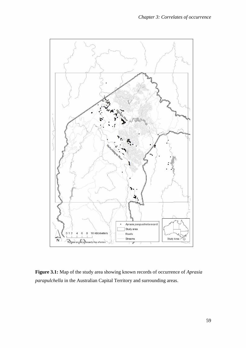
Chapter 3: Correlates of occurrence
59
Figure 3.1: Map of the study area showing known records of occurrence of Aprasia
parapulchella in the Australian Capital Territory and surrounding areas.
Chapter 3: Correlates of occurrence
60
Selection of modelling package
Whilst there is generally good survey coverage for A. parapulchella in the ACT, no
systematic survey of the whole study area has been conducted. Therefore, I selected the
presence-only SDM package, MaxEnt (Phillips et al. 2004) for the modelling exercise.
MaxEnt is widely used and known to be one of the best performing SDM packages
(Elith et al. 2006; Elith et al. 2011; Hernandez et al. 2006).
Data layer selection
I obtained environmental layers and presence data for A. parapulchella from the
ACT Government. This data included wildlife atlas records as well as records from
other surveys. Most of these data were digitised points based on grid references
recorded during field surveys or digitised locations transferred from physical maps
where records were marked to digital form (Jones 1992; Jones 1999; Osborne and
Coghlan 2004; Osborne and McKergow 1993). These data were supplemented
considerably with additional data (258 records) collected using GPS during extensive
surveys conducted within the study area (Osborne and Wong 2010; D. Wong
unpublished data; Wong and Osborne 2010). The accuracy of the data is likely to have
varied, with records collected before the advent of GPS more likely to be subject to
positional error. However, the data were checked for plausibility and records that
appeared likely to be erroneous were excluded. The initial set of environmental layers
consisted of topographical layers derived from a 25m digital elevation model (DEM) of
the Australian Capital Territory region and climatic layers for mean monthly maximum
and minimum temperature and mean monthly rainfall calculated using ESOCLIM
(Houlder et al. 2000). This application derives climatic surfaces based on climate data
and a DEM. Solar radiation was derived in ArcGIS 9.3.1 (ESRI 1999 - 2009) using the
Chapter 3: Correlates of occurrence
61
25m DEM. Environmental layers were selected based on their ecological relevance for
the species (Austin 2002). Variables that were very highly inter-correlated [r > 0.75]
(Appendix 3) were removed. Whilst MaxEnt incorporates L1 regularization, that is
known to perform well in feature selection (Hastie et al. 2009) some level of variable
pre-selection (i.e. using ecologically relevant variables) is considered prudent (Elith et
al. 2011).
Previous studies have suggested that A parapulchella is unlikely to be found in
areas that have undergone very high levels of agricultural modification (Jones 1999;
Osborne and McKergow 1993). Therefore, I included agricultural modification in the
model, and this was done in the following way.
Native summer growing grasses are gradually replaced by exotic winter growing
species as levels of grazing and fertiliser addition increase in mesic areas (Groves et al.
2003; Stuwe and Parsons 1977). Therefore, for the agricultural modification variable, I
used a vegetation classification provided by the New South Wales Office of
Environment and Heritage (Environmental Research and Information Consortium
2001). This classification used the differences in spectral reflectance between remotely
sensed images in spring and summer to discriminate between areas dominated by C4
(primarily summer growing native) and C3 (primarily winter growing exotic) grasses
and was based on the methods developed by Langston (1996). The classification had
been verified in the field and since refined based on known sites in New South Wales
(Environmental Research and Information Consortium 2001, R. Rehwinkel, NSW
Office of Environment and Heritage pers. comm.). I reclassified the original
classification of 23 classes into four classes: native grassy areas (C4 dominated),
woodland, exotic (or degraded native) grassy areas and unknown. Some areas of the
Chapter 3: Correlates of occurrence
62
extent (forested areas of > 30 % tree cover, and urban area) had been masked out when
the original classification was produced, but since there are no records of the species
from forested sites (except for one site at Black Mountain which is located in an open
area within open forest), this was not considered to be a limitation.
Relationships between A. parapulchella and the environmental variables of
geology, soils, slope, solar radiation have all been described previously (Jones 1999;
Osborne et al. 1991). Therefore, these variables were included in the model. Solar
radiation was included in the initial model but was subsequently dropped because it
made little contribution. Elevation was highly correlated with temperature. Because
variables with a direct physiological effect on species distribution are generally
preferable to indirect variables (Austin 2002; but see Van Niel et al. 2004), I excluded
elevation from the analysis in favour of temperature. As A. parapulchella is thought to
disperse and breed and in spring (Jones 1999), I included mean minimum temperature in
October and mean monthly rainfall in October in the model. Minimum temperature was
selected over maximum temperature because low temperatures are more limiting to
reptiles than high temperatures (Heatwole and Taylor 1987).
Environmental layers were prepared in ArcGIS 9.3.1 (ESRI 1999 - 2009). Raster
files were converted to ASCII data layers with a cell size of 25m in GDA 1994 Zone 55
MGA projection (Koy 2009).
Model running and optimisation
In order to reduce the likelihood of sampling bias affecting the final model, any
records that were less than approximately 30m from another record were removed. This
was performed manually using ArcGIS 9.3.1. The model was run with 50% of the
Chapter 3: Correlates of occurrence
63
records (168 records) allocated for model training and the remaining 50% used to test
the model. The training and test data were selected randomly by MaxEnt. Ten replicates
of the model were run and the average of these models used in the analysis.
Assessment of the model
The model evaluation measures of area under the receiver operating curve [AUC]
(Hanley and NcNeil 1982; Pearce and Ferrier 2000) and gain (Phillips 2006) were
assessed. The gain is a measure of the improvement in penalized average log likelihood
compared to a null model (Elith et al. 2011). Higher values of AUC and gain indicated
better model performance. The visual representation of the model was then interpreted.
The contribution of each of the variables and response curves/plots were also
interpreted. MaxEnt provides two response curves/plots for each variable. The marginal
response curve/plot shows how the logistic prediction of the MaxEnt model changes as
a given environmental variable is varied (and all other variables are kept at their sample
average). The other set of response curves/plots (referred hitherto as individual response
curves/plots) represent MaxEnt models for each of the variables. The latter curves/plots
may be easier to interpret if the predictor variables are strongly correlated (Phillips
2006).
Results
The MaxEnt model evaluation results are reported in Table 3.1. The AUC figures
suggest that the model had high predictive ability. AUC values over 0.90 are considered
to be high (Manel et al. 2001; Swets 1988). The gain measures the likelihood of the
samples. The average sample likelihood equals the exponential of the gain [exp(gain)].
Therefore the gain measures indicate that the sample likelihood was ≈ 4.3 to 5.6 times
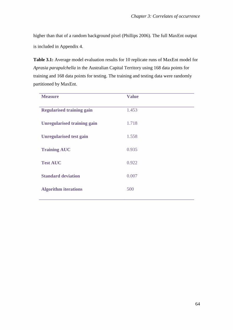
Chapter 3: Correlates of occurrence
64
higher than that of a random background pixel (Phillips 2006). The full MaxEnt output
is included in Appendix 4.
Table 3.1: Average model evaluation results for 10 replicate runs of MaxEnt model for
Aprasia parapulchella in the Australian Capital Territory using 168 data points for
training and 168 data points for testing. The training and testing data were randomly
partitioned by MaxEnt.
Measure Value
Regularised training gain 1.453
Unregularised training gain 1.718
Unregularised test gain 1.558
Training AUC 0.935
Test AUC 0.922
Standard deviation 0.007
Algorithm iterations 500
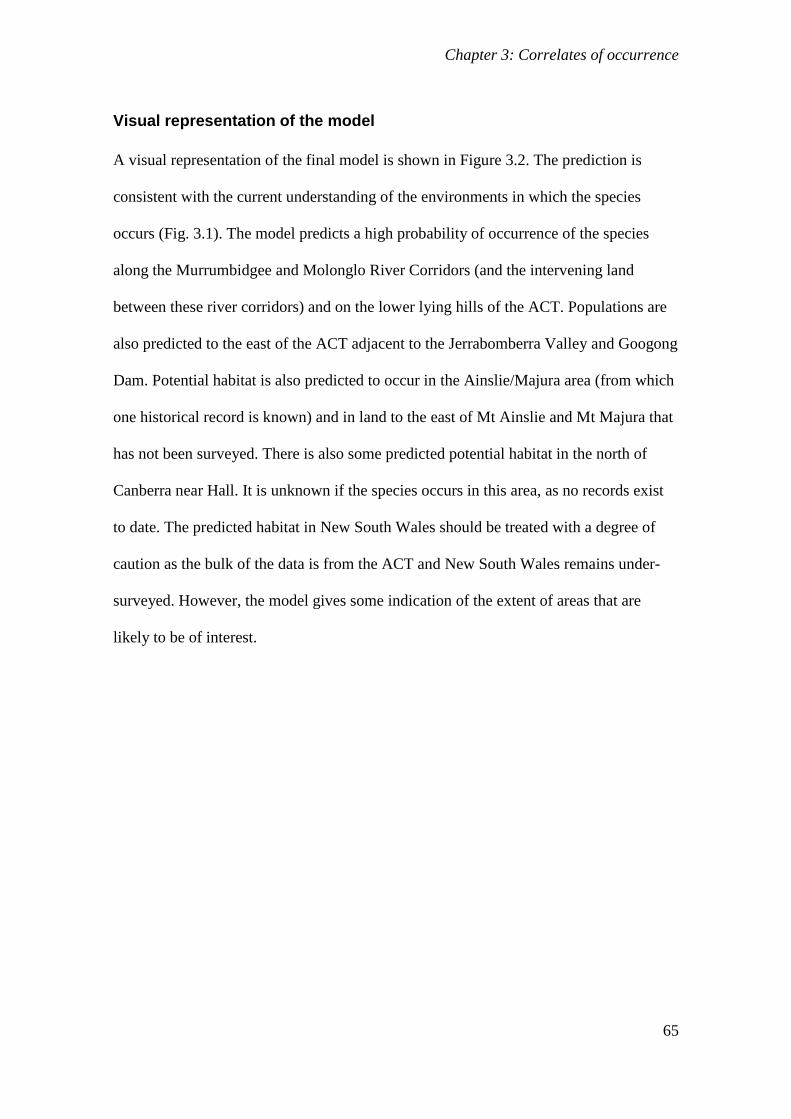
Chapter 3: Correlates of occurrence
65
Visual representation of the model
A visual representation of the final model is shown in Figure 3.2. The prediction is
consistent with the current understanding of the environments in which the species
occurs (Fig. 3.1). The model predicts a high probability of occurrence of the species
along the Murrumbidgee and Molonglo River Corridors (and the intervening land
between these river corridors) and on the lower lying hills of the ACT. Populations are
also predicted to the east of the ACT adjacent to the Jerrabomberra Valley and Googong
Dam. Potential habitat is also predicted to occur in the Ainslie/Majura area (from which
one historical record is known) and in land to the east of Mt Ainslie and Mt Majura that
has not been surveyed. There is also some predicted potential habitat in the north of
Canberra near Hall. It is unknown if the species occurs in this area, as no records exist
to date. The predicted habitat in New South Wales should be treated with a degree of
caution as the bulk of the data is from the ACT and New South Wales remains under-
surveyed. However, the model gives some indication of the extent of areas that are
likely to be of interest.
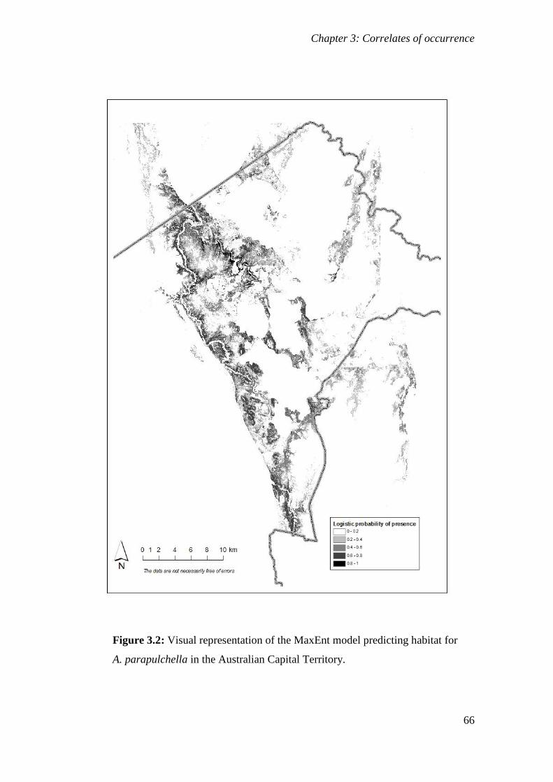
Chapter 3: Correlates of occurrence
66
Figure 3.2: Visual representation of the MaxEnt model predicting habitat for
A. parapulchella in the Australian Capital Territory.
Chapter 3: Correlates of occurrence
67
Contribution of variables
The MaxEnt estimates of variable contribution and jack-knife analysis showed some
differences (Table 3.2; Appendix 4) showed some differences. This is likely to be due to
inter-correlation of variables (Appendix 3). For the jack-knife analysis (Appendix 4),
whilst geology was the contributed most to the gain in isolation from the other
variables, omission of the soil variable led to the greatest decrease in gain, suggesting
that the soils variable accounts for the highest amount of variation that is not explained
by other variables. The analysis of variable contribution estimates (Table 3.2) indicated
that the soils variable contributed nearly 30% to the model. Slope and geology
contributed similar amounts (approximately 17%) but the permutation importance of the
geology variable was higher (23.6% compared with 12.7% for slope). The contributions
of average minimum temperature in October and average rainfall in October were both
between approximately 10% and 15% and the agricultural modification layer
contributed approximately 8% of the variation (Table 3.2). These results should be
interpreted with some caution as there is some correlation between the predictor
variables (Appendix 3).
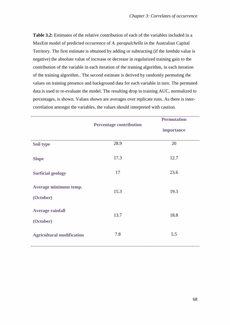
Chapter 3: Correlates of occurrence
68
Table 3.2: Estimates of the relative contribution of each of the variables included in a
MaxEnt model of predicted occurrence of A. parapulchella in the Australian Capital
Territory. The first estimate is obtained by adding or subtracting (if the lambda value is
negative) the absolute value of increase or decrease in regularized training gain to the
contribution of the variable in each iteration of the training algorithm, in each iteration
of the training algorithm.. The second estimate is derived by randomly permuting the
values on training presence and background data for each variable in turn. The permuted
data is used to re-evaluate the model. The resulting drop in training AUC, normalized to
percentages, is shown. Values shown are averages over replicate runs. As there is inter-
correlation amongst the variables, the values should interpreted with caution.
Percentage contribution
Permutation
importance
Soil type 28.9 20
Slope 17.3 12.7
Surficial geology 17 23.6
Average minimum temp.
(October)
15.3 19.3
Average rainfall
(October)
13.7 18.8
Agricultural modification 7.8 5.5
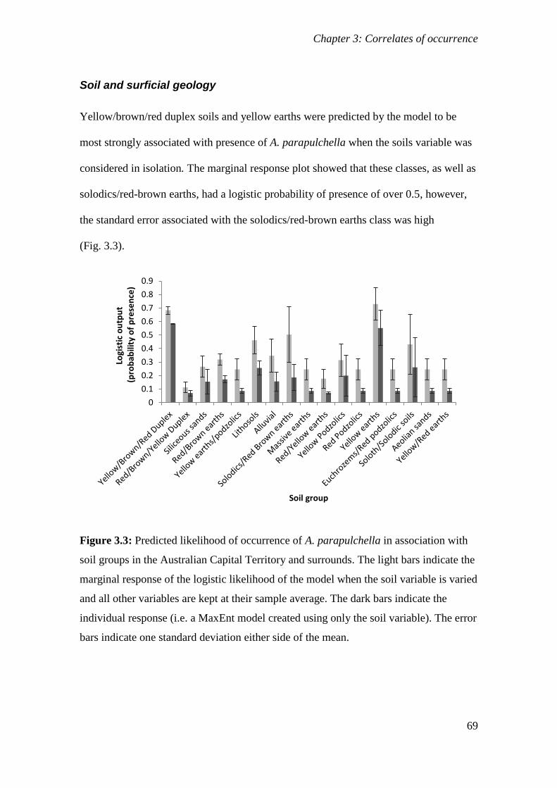
Chapter 3: Correlates of occurrence
69
Soil and surficial geology
Yellow/brown/red duplex soils and yellow earths were predicted by the model to be
most strongly associated with presence of A. parapulchella when the soils variable was
considered in isolation. The marginal response plot showed that these classes, as well as
solodics/red-brown earths, had a logistic probability of presence of over 0.5, however,
the standard error associated with the solodics/red-brown earths class was high
(Fig. 3.3).
Figure 3.3: Predicted likelihood of occurrence of A. parapulchella in association with
soil groups in the Australian Capital Territory and surrounds. The light bars indicate the
marginal response of the logistic likelihood of the model when the soil variable is varied
and all other variables are kept at their sample average. The dark bars indicate the
individual response (i.e. a MaxEnt model created using only the soil variable). The error
bars indicate one standard deviation either side of the mean.
0
0.1
0.2
0.3
0.4
0.5
0.6
0.7
0.8
0.9
Logi
stic
ou
tpu
t (
pro
bab
ility
of
pre
sen
ce)
Soil group
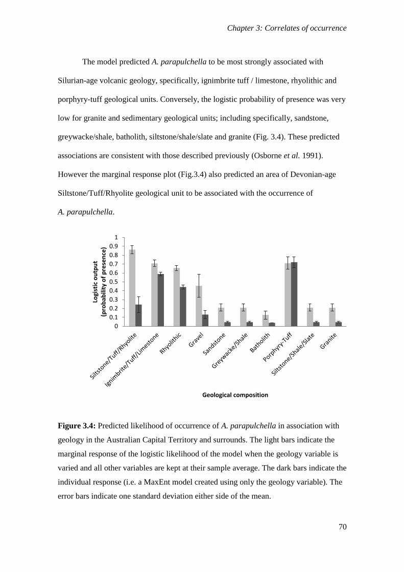
Chapter 3: Correlates of occurrence
70
The model predicted A. parapulchella to be most strongly associated with
Silurian-age volcanic geology, specifically, ignimbrite tuff / limestone, rhyolithic and
porphyry-tuff geological units. Conversely, the logistic probability of presence was very
low for granite and sedimentary geological units; including specifically, sandstone,
greywacke/shale, batholith, siltstone/shale/slate and granite (Fig. 3.4). These predicted
associations are consistent with those described previously (Osborne et al. 1991).
However the marginal response plot (Fig.3.4) also predicted an area of Devonian-age
Siltstone/Tuff/Rhyolite geological unit to be associated with the occurrence of
A. parapulchella.
Figure 3.4: Predicted likelihood of occurrence of A. parapulchella in association with
geology in the Australian Capital Territory and surrounds. The light bars indicate the
marginal response of the logistic likelihood of the model when the geology variable is
varied and all other variables are kept at their sample average. The dark bars indicate the
individual response (i.e. a MaxEnt model created using only the geology variable). The
error bars indicate one standard deviation either side of the mean.
0
0.1
0.2
0.3
0.4
0.5
0.6
0.7
0.8
0.9
1
Logi
stic
ou
tpu
t (p
rob
abili
ty o
f p
rese
nce
)
Geological composition
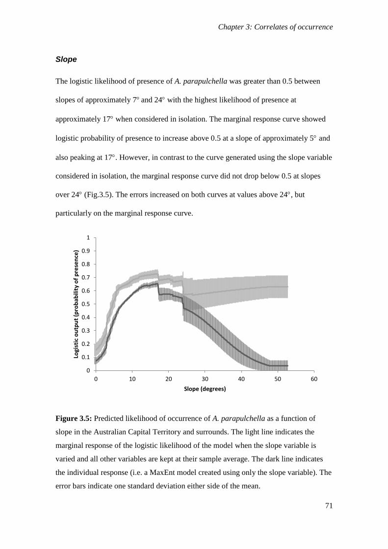
Chapter 3: Correlates of occurrence
71
Slope
The logistic likelihood of presence of A. parapulchella was greater than 0.5 between
slopes of approximately 7 and 24 with the highest likelihood of presence at
approximately 17 when considered in isolation. The marginal response curve showed
logistic probability of presence to increase above 0.5 at a slope of approximately 5 and
also peaking at 17. However, in contrast to the curve generated using the slope variable
considered in isolation, the marginal response curve did not drop below 0.5 at slopes
over 24 (Fig.3.5). The errors increased on both curves at values above 24, but
particularly on the marginal response curve.
Figure 3.5: Predicted likelihood of occurrence of A. parapulchella as a function of
slope in the Australian Capital Territory and surrounds. The light line indicates the
marginal response of the logistic likelihood of the model when the slope variable is
varied and all other variables are kept at their sample average. The dark line indicates
the individual response (i.e. a MaxEnt model created using only the slope variable). The
error bars indicate one standard deviation either side of the mean.
0
0.1
0.2
0.3
0.4
0.5
0.6
0.7
0.8
0.9
1
0 10 20 30 40 50 60
Logi
stic
ou
tpu
t (p
rob
abili
ty o
f p
rese
nce
)
Slope (degrees)
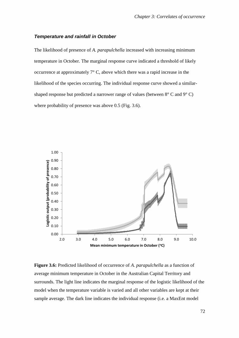
Chapter 3: Correlates of occurrence
72
Temperature and rainfall in October
The likelihood of presence of A. parapulchella increased with increasing minimum
temperature in October. The marginal response curve indicated a threshold of likely
occurrence at approximately 7° C, above which there was a rapid increase in the
likelihood of the species occurring. The individual response curve showed a similar-
shaped response but predicted a narrower range of values (between 8° C and 9° C)
where probability of presence was above 0.5 (Fig. 3.6).
Figure 3.6: Predicted likelihood of occurrence of A. parapulchella as a function of
average minimum temperature in October in the Australian Capital Territory and
surrounds. The light line indicates the marginal response of the logistic likelihood of the
model when the temperature variable is varied and all other variables are kept at their
sample average. The dark line indicates the individual response (i.e. a MaxEnt model
0.00
0.10
0.20
0.30
0.40
0.50
0.60
0.70
0.80
0.90
1.00
2.0 3.0 4.0 5.0 6.0 7.0 8.0 9.0 10.0
Logi
stic
ou
tpu
t (p
rob
abili
ty o
f p
rese
nce
)
Mean minimum temperature in October (oC)
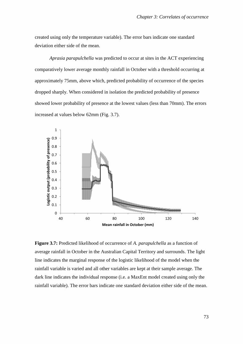
Chapter 3: Correlates of occurrence
73
created using only the temperature variable). The error bars indicate one standard
deviation either side of the mean.
Aprasia parapulchella was predicted to occur at sites in the ACT experiencing
comparatively lower average monthly rainfall in October with a threshold occurring at
approximately 75mm, above which, predicted probability of occurrence of the species
dropped sharply. When considered in isolation the predicted probability of presence
showed lower probability of presence at the lowest values (less than 70mm). The errors
increased at values below 62mm (Fig. 3.7).
Figure 3.7: Predicted likelihood of occurrence of A. parapulchella as a function of
average rainfall in October in the Australian Capital Territory and surrounds. The light
line indicates the marginal response of the logistic likelihood of the model when the
rainfall variable is varied and all other variables are kept at their sample average. The
dark line indicates the individual response (i.e. a MaxEnt model created using only the
rainfall variable). The error bars indicate one standard deviation either side of the mean.
0
0.1
0.2
0.3
0.4
0.5
0.6
0.7
0.8
0.9
1
40 60 80 100 120 140
Logi
stic
ou
tpu
t (p
rob
abili
ty o
f p
rese
nce
)
Mean rainfall in October (mm)
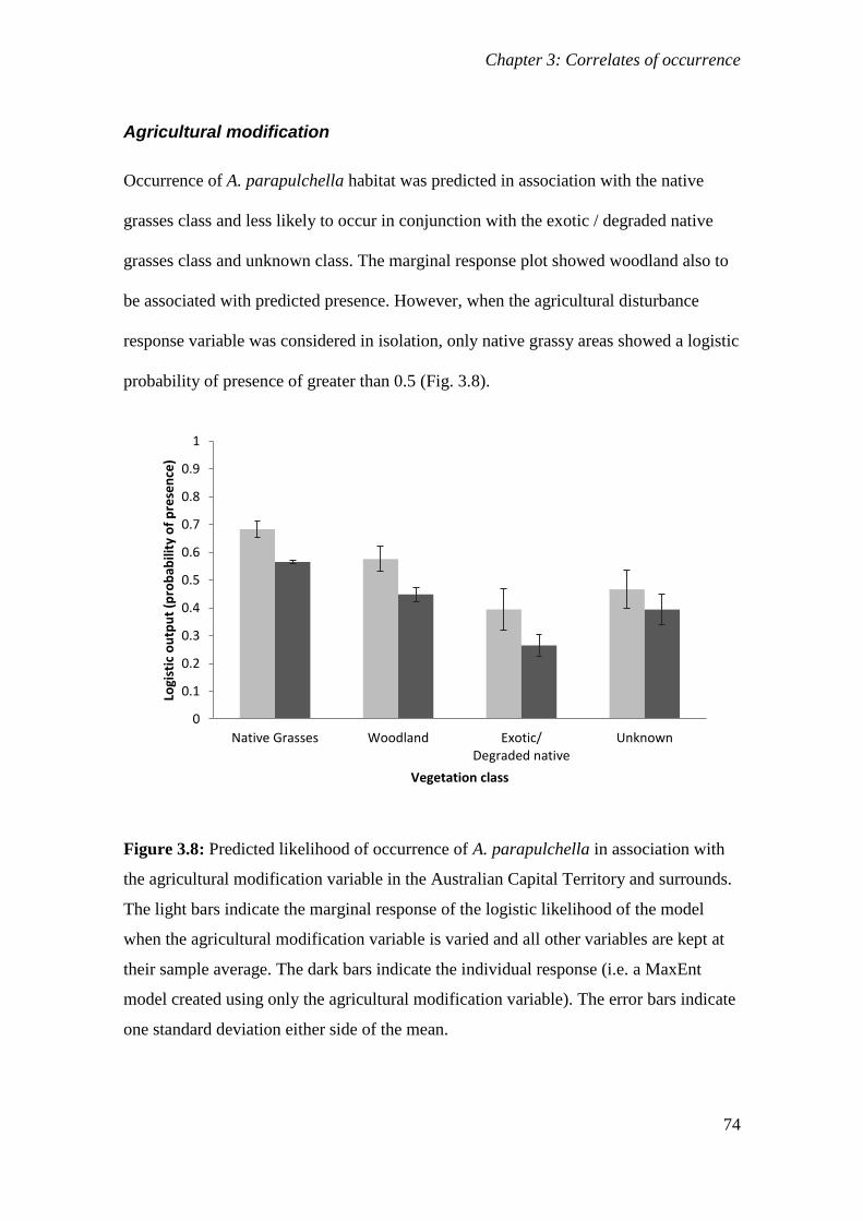
Chapter 3: Correlates of occurrence
74
Agricultural modification
Occurrence of A. parapulchella habitat was predicted in association with the native
grasses class and less likely to occur in conjunction with the exotic / degraded native
grasses class and unknown class. The marginal response plot showed woodland also to
be associated with predicted presence. However, when the agricultural disturbance
response variable was considered in isolation, only native grassy areas showed a logistic
probability of presence of greater than 0.5 (Fig. 3.8).
Figure 3.8: Predicted likelihood of occurrence of A. parapulchella in association with
the agricultural modification variable in the Australian Capital Territory and surrounds.
The light bars indicate the marginal response of the logistic likelihood of the model
when the agricultural modification variable is varied and all other variables are kept at
their sample average. The dark bars indicate the individual response (i.e. a MaxEnt
model created using only the agricultural modification variable). The error bars indicate
one standard deviation either side of the mean.
0
0.1
0.2
0.3
0.4
0.5
0.6
0.7
0.8
0.9
1
Native Grasses Woodland Exotic/Degraded native
Unknown
Logi
stic
ou
tpu
t (p
rob
abili
ty o
f p
rese
nce
)
Vegetation class
Chapter 3: Correlates of occurrence
75
Discussion
Model performance
The results indicate that the model performs very well (Table 3.1). AUC values of over
0.90 are considered to have high predictive ability (Manel et al. 2001; Swets 1988).
There are some possible measures that could be taken to improve the model. A remotely
sensed classification that discriminated areas of rock would be very valuable as a
predictor variable. In addition, further surveys of areas surrounding the ACT are needed
before the model can be applied beyond the ACT border with high levels of confidence.
Another limitation of the model is the age of the agricultural modification layer
(Environmental Research and Information Consortium 2001). Whilst this is not seen to
be a major limitation, it is likely that updating the layer would produce some minor
improvements to the model.
Visual representation of the model
The areas of high likelihood of occurrence were consistent with current knowledge of
where the species occurs in the ACT. In addition, areas of potential occurrence were
identified in the north of the ACT (in areas close to Hall); in the north-eastern parts of
the ACT (Ainslie/Majura Nature Reserves and nearby areas); and to the northwest and
east of the ACT (Fig. 3.2). It should be noted that there are relatively few data points in
NSW, so it is possible that the model under-represents areas of potential habitat outside
of the ACT.
Contribution of variables
The contribution of the variables is consistent with the current knowledge of
A. parapulchella (Wong et al. 2011). For example, the occurrence of A. parapulchella is
Chapter 3: Correlates of occurrence
76
known to be strongly linked to the occurrence of Silurian volcanic geology (Osborne et
al. 1991). However, the modelling has helped to further quantify the relative
contribution of the important variables at the regional scale. The contribution is also
consistent with theory relating to the scale at which environmental factors affect
primary environmental resources (i.e. heat, light, water and mineral nutrients) and
hierarchical patterns of species distribution [e.g. in toto distribution, population and
metapopulation, pair or colony and single organism] (Guisan and Thuiller 2005;
Mackey and Lindenmayer 2001). Geology, soil type and climatic factors affect
distributions at broad scales (global-scale to nano-scale) and may be associated with
biogeographical patterns and limiting climatic factors. Thus they are likely to exert an
influence over the broader distribution of the species (Guisan and Thuiller 2005;
Mackey and Lindenmayer 2001). Slope is likely to influence meso-scaled climatic
variables at the intermediate topo-scale (Mackey and Lindenmayer 2001). Disturbance
factors act on parts of the broader climatic envelope of a species and influence resources
at the local scale [micro-scale] (Guisan and Thuiller 2005). Therefore, it is likely that
the agricultural modification variable has the lowest contribution to the model as it is
providing fine-scale refinements, rather than broad scale changes to the model.
Nonetheless, these refinements are likely to be important for a species such as
A. parapulchella as fine-resolution local predictors can improve prediction for species
which are sessile or display limited mobility (Guisan and Thuiller 2005). Another
possible reason for the lower estimated contribution of the agricultural modification
variable is that there is an interaction with another variable or variables such as geology
slope or soils. As the soils, geology and agricultural modification variables are all
categorical, it is difficult to disentangle the exact nature of the interactions.
Chapter 3: Correlates of occurrence
77
Habitat correlates
The results indicate that MaxEnt is useful in characterising habitat relationships;
however, it is often difficult to decide whether to use the marginal response curve or the
curve of the variable in question in isolation. Interpretation of the MaxEnt plots and
curves can be challenging as interactions between variables may influence their
response. In interpreting the plots, it was helpful to visually inspect the environmental
layers in a Geographical Information System (GIS) in order to clarify relationships. In
some cases, the relatively small area of some values of the environmental layers may
lead to a seemingly strong logistic probability of occurrence, but this must be
interpreted in the context of the environmental layer.
Soil and surficial geology
Most of the A. parapulchella records in the ACT coincide with the yellow/brown/red
duplex soils (Fig. 3.3). This soil group does however coincide with the Silurian age
volcanic rock types that A. parapulchella is also closely associated with. The strong
response to the yellow earths soil group may result from the fact these soils occur in a
relatively small area within the ACT, much of which is located in close proximity to the
yellow/brown/red duplex group. This is could also be the case for red/brown earths
group. There has been no specific investigation of the relationship between soil
conditions and the occurrence or abundance of A. parapulchella. Given the seemingly
strong response suggested by this study, further investigation of this topic would help to
clarify the extent to which soil type and conditions are important to A. parapulchella.
The identification of type of surficial geology in the jack-knife analysis
(Appendix 4) as the major variable of importance is consistent with the earlier findings
Chapter 3: Correlates of occurrence
78
within the ACT, that the presence of A. parapulchella is strongly associated with
Silurian-age volcanic geological units. Inspection of the geology layer revealed that
most of the records correspond with the rhyolithic and ignimbrite/tuff/limestone and
porphyry-tuff geological classes. Surface rocks in areas underlain by these geological
units appear to be conducive to the requirements of A. parapulchella. They are often
small to medium-sized (approximately 10cm – 30cm long) and are shallowly embedded.
Therefore, they are likely to be easily colonised by ants. The model also revealed an
association between A. parapulchella and a Devonian-age geological unit for the first
time in the ACT. The population that occurs in this location appears to be an outlying
population within the context of the ACT. Therefore, further analysis of the attributes of
this population may reveal interesting findings.
The model predicted that the species was not likely to occur on alluvial,
sedimentary or granite geological units [gravel, sandstone, greywacke/shale, batholith,
siltstone/shale/slate and granite] (Fig. 3.4). There is only one record in the Australian
Capital Territory (on Black Mountain) that is underlain by sedimentary geology [quartz
sandstone] (Wong et al. 2011) and no specimens have been recorded in areas underlain
by granodiorite in the ACT (Osborne et al. 1991). Granite areas tend to feature large
embedded tors and boulders or thin exfoliated sheets, rather than the small, relatively
lightly embedded blocks that A. parapulchella appears to favour in the ACT. However,
at Tarcutta in New South Wales, A. parapulchella has been recorded under exfoliated
granite (Jones 1992). Therefore, there may be other factors involved in the ACT. For
example, much of the area underlain by granodiorite occurs in the higher elevation areas
of the ACT.
Chapter 3: Correlates of occurrence
79
It is possible that biogeographical factors relating to geological processes also
influence on the apparent relationship between occurrence of A. parapulchella and
geology type. For example, reactivation of faults in the ACT region in the Cenozoic Era
(65.5 Ma to present) combined with block tilting and subsequent erosion are believed to
have led to the current day low and high elevation areas in the ACT (Finlayson 2008).
Indeed, all the known records appear to be located in conjunction with the lower lying
Canberra Rift structure constrained largely by the Murrumbidgee Fault and Queanbeyan
Fault. Other faults in the region that may have influenced the distribution of
A. parapulchella in the ACT include the Winslade Fault and the Deakin Fault. Although
the faulting is not likely to have influenced the distribution of the species directly, the
legacy of these events on the geomorphology of the area may be important. The
contribution of geological activity in influencing the population located in native
vegetation at Uriarra Forest is of particular interest. This population is constrained by a
number of fault lines within a thin area of Mountain Creek Volcanic. This population
appears to be somewhat of an outlier in the context of the ACT.
Slope
The predicted response of A. parapulchella to slope (Fig. 3.5) was roughly consistent
with the findings of Jones (1992) who found that records were most frequently found at
sites with slopes of between 10° and 14°. Very gently sloping areas were predicted to
have a low probability of supporting the species. This is likely to be because flat areas
such as grasslands at valley bottoms often do not contain surface rock, whilst hill slopes,
because of the erosional processes that have shaped them, often feature suitable surface
rock. However, areas with gentle slopes on hilltops or hillocks are still likely to support
Chapter 3: Correlates of occurrence
80
the species. The response curve for slope in isolation showed a similar pattern to that
observed by Jones (1992). That is, a drop in the probability of occurrence of
A. parapulchella in steeper locations. The marginal response curve, whilst still showing
some threshold behaviour at 24°, did not drop below 0.5 even when slopes were > 20°.
These values are underrepresented in surveys and as slopes approached 20° errors
associated with the response curves increased so, further work may be required to
clarify these relationships. However, very steep slopes may be less conducive to the
formation of suitable rocks as non-embedded rocks may be more subject to the effects
of gravity at such sites compared with comparatively gentler slopes.
Temperature and rainfall in October
Inspection of the environmental layer for mean minimum temperature in October using
GIS revealed that the marginal response curve (Fig. 3.6) better approximated the actual
presence of A. parapulchella records. The association between A. parapulchella and
higher minimum temperature in October is also expected as the known distribution of
A. parapulchella coincides with comparatively lower altitude areas which are subject to
milder temperatures. Visual inspection of the layer using GIS revealed that the apparent
drop in the predicted likelihood of occurrence of A. parapulchella at the highest
temperatures is most likely to be attributed to those values representing only a very
small percentage of the study area in an area that is under-surveyed. It is unclear
whether the main factor that restricts A. parapulchella to the lower lying areas of the
ACT is geology (much of the higher elevation areas are underlain by granite which is
thought to be unsuitable for the species) or temperature; however, it is likely that both
factors play a role. Cooler, higher elevation areas are also often dominated by forest
vegetation communities, which are likely to further limit solar radiation reaching the
Chapter 3: Correlates of occurrence
81
ground and therefore, limit opportunities for thermoregulation (Pringle et al. 2003). A.
parapulchella has not been recorded at cold-air drainage grassland sites, probably
because of the lack of suitable rock at these sites. However, the species has been
recorded in rocky sites fringing grasslands [e.g. West Jerrabomberra Grassland Reserve]
(ACT Parks Conservation and Lands Vertebrate Atlas). It is likely that the fossorial
nature of the species allows it a degree of protection from extreme temperatures.
Both the individual and marginal response curves (Fig. 3.7) showed threshold
behaviour at approximately 75mm of October rainfall. Rainfall values higher than this
correspond with the higher elevation areas in the ACT. The lower predicted probability
of presence of A. parapulchella at the lowest rainfall values (less than 70mm) observed
in the response curve for rainfall in October in isolation coincides with lower lying areas
of Canberra and areas to the East of Canberra around Googong Reservoir. In Canberra,
many of the areas that coincide with these values are cold-air drainage grassland
ecosystems that lack rocks. The neighbouring areas of New South Wales (close to
Googong Reservoir) also experience comparatively low rainfall. These areas contain
suitable rocky areas but are under surveyed.
Agricultural modification
The response of A. parapulchella to agricultural modification (Fig. 3.8) was consistent
with previous studies that the species is associated with areas dominated by native
grasses (Jones 1999; Osborne et al. 1991). When the agricultural modification layer was
considered in isolation, only the native grasses category had a logistic predicted
probability of occurrence of greater than 0.5. For the marginal response plot, the
woodland category was also above 0.5. Knowledge to date (Barrer 1992; Osborne and
McKergow 1993) suggests that A. parapulchella is less likely to occur in areas with
Chapter 3: Correlates of occurrence
82
high percentage cover of trees or shrubs. However, the species has been found in more
open areas with suitable rock within forest and woodland (Wong et al. 2011). The lower
predicted likelihood of sites dominated by exotic vegetation containing habitat is
consistent with previous findings (Jones 1999; Osborne et al. 1991; Osborne and
McKergow 1993). The likelihood of predicted habitat coinciding with the ‘unknown’
vegetation class was also low. Inspection of the agricultural modification layer using
GIS suggested that that this class is most likely to be associated with exotic grass or
degraded native grasses – this is based on its regular occurrence in areas known to be
dominated by exotic or degraded native areas as well as its occurrence in close
proximity to areas classified as being exotic. As the agricultural modification layer uses
discrimination between C3 and C4 grass species as the basis for classification, some of
the sites in the ‘exotic/degraded native’ category may be degraded native sites
dominated by C3 grasses such as Austrostipa spp. or Austrodanthonia spp. This should
be considered when interpreting the model as some of these sites may be occupied by
A. parapulchella.
Interpretation of response
MaxEnt has a range of advantages. It is a flexible method that can incorporate
interactions between variables and incorporates methods that reduce the likelihood of
over-fitting models through the use of L1 regularization (Elith et al. 2011). However,
the power of its ability to fit complex functions and incorporate interactions using
“features” (see Elith et al 2011) is also one drawback when it comes to interpretation of
correlates of occurrence. It is helpful for achieving a better understanding of the
correlates of occurrence of species, but there is some uncertainty associated with the
response curves or plots and this should be taken into account when interpreting the
Chapter 3: Correlates of occurrence
83
output. The provision of a marginal response curve as well as the individual response
curve by MaxEnt sometimes makes it more difficult to draw clear conclusions about the
relationship between the variables and occurrence of the species of interest. The lack of
the ability of MaxEnt to give a clear figure of probability of presence is a recent
criticism that has been raised (Royle et al. 2012). Interrogation of the data is also
necessary in order to assess the plausibility of the response curves or plots.
Conclusion
MaxEnt can be a powerful tool for characterising correlates of species occurrence. This
study has revealed that MaxEnt has the potential to effectively confirm and refine
knowledge about species correlates of occurrence. It also offers the advantage of being
able to characterise predicted occurrence in association with variables that are difficult
to measure effectively in the field (e.g. climatic variables). Nonetheless, caution should
be taken when interpreting the results and interactions between variables can make
interpretation difficult.
Potential new areas of occurrence of A. parapulchella in the ACT have been
identified in this study and further survey is needed to determine whether the species
occurs in these areas. In addition, the modelling revealed a new association between
A. parapulchella and an early Devonian geological unit and described relationships
between the occurrence of A. parapulchella and temperature and rainfall. The findings
are likely to aid conservation planning efforts for the species by identifying areas likely
to be occupied as well as giving insights into how the probability of occurrence of the
species is influenced by environmental factors.
Chapter 3: Correlates of occurrence
84
Acknowledgements
I thank Mike Austin of CSIRO, Andre Zerger of the Australian Bureau of Meteorology
and Margaret Kitchin of Australian Capital Territory Conservation Planning and
Research for advice regarding modelling and for providing data layers. Rainer
Rehwinkel of the New South Wales Office of Environment and Heritage provided the
remote sensing data and helpful information regarding the agricultural modification
data. Annabel Smith, Ingrid Stirnemann, Nicole Maron, David Leigh, Percy Wong and
Elisabeth Wong provided useful comments on manuscript. Finally, I thank the
Australian Capital Territory Government for providing funding to undertake the project,
data layers and specimen records. This study was authorised by the University of
Canberra Committee for Ethics in Animal Experimentation (project authorisation code
CEAE08-17). Field work was carried out under licence, in accordance with the Nature
Conservation Act 1980 (Licence no. LT2008311).
Chapter 4: SDMs and agricultural modification
85
4. Species distribution modelling for a disturbance-
sensitive lizard: agricultural modification matters
Abstract
The ecological niche of a species is determined by a number of environmental
factors (climate factors, resource factors, disturbances and interactions with other
species). Species distribution models attempt to encapsulate this ecological niche and
represent it spatially. Human-induced disturbance is a major driver of species decline
and, therefore, affects species distribution. Nonetheless, relatively few species
distribution models incorporate disturbance.
I incorporated agricultural modification into a species distribution model for the
Pink-tailed Worm-lizard (Aprasia parapulchella) (Pygopodidae); a habitat specialist,
relying on sites containing surface rock and dominated by native grasses. I constructed
MaxEnt models with and without agricultural modification included as a factor. I
assessed the predictive ability of the models, area of classes of vegetation predicted, and
agreement with known habitat mapped in the field.
Inclusion of agricultural modification improved model performance and led to
more native vegetation and less exotic vegetation being predicted as suitable for
A. parapulchella. Analysis of a sub-area that contained a range of levels of modification
within the greater study area indicated that inclusion of agricultural modification led to
a model with slightly higher omission rate but markedly lower commission index (i.e.
Chapter 4: SDMs and agricultural modification
86
fewer false positives) and a significantly lower average likelihood of predicting false
positives (t = 2.32; p = 0.021). Expert assessment of the model in association with
mapped habitat also suggested that inclusion of agricultural modification improved
prediction of suitable habitat. Thresholds suggested by MaxEnt over-estimated suitable
habitat for the species in the sub-area. Taking into account the appropriate caveats, it is
tentatively estimated that agricultural modification has led to the destruction or decline
of approximately 30-35 % of optimal habitat in the sub-area of study and approximately
20% of optimal habitat across the Australian Capital Territory.
These findings will be relevant to those concerned with threatened species
planning and management, particularly at finer spatial scales. Failure to account for
disturbance adequately could be a critical issue for disturbance sensitive species such as
A. parapulchella or for less mobile species with poor dispersal ability. Therefore, I
recommend that disturbance factors be incorporated into species distribution modelling,
or at least explored, wherever possible.
Chapter 4: SDMs and agricultural modification
87
Introduction
The concept of ecological niche (Chase and Leibold 2003; Elton 1927; Grinnell
1917; Hutchinson 1957; Pulliam 2000; Vandermeer 1972) addresses a fundamental
question in ecology: how are species distributed in the environment and what limits
their distribution? Species distribution models (SDMs) ( Elith et al. 2006; Guisan and
Zimmermann 2000) draw on ecological niche theory (Guisan and Thuiller 2005; Hirzel
and Le Lay 2008). SDMs link known occurrence data with environmental data to
produce spatially-explicit predictions of the occurrence of species. They are commonly
applied in predicting the occurrence or habitat of species or communities and are used to
support conservation management and planning (Ferrier et al. 2002; Guisan and
Thuiller 2005; Loiselle et al. 2003; Pearce and Lindenmayer 1998; Pearson 2007;
Raxworthy et al. 2003). SDMs usually attempt to incorporate factors that fall into one or
more of the following three groups: limiting factors, relating to the eco-physiological
limits of a species (e.g. climatic factors); natural and human-caused disturbances; and
resources available to an organism (e.g. food, water and shelter) (Guisan and Thuiller
2005). However, the link between species distribution modelling and ecological theory
is often not explicitly integrated into modelling exercises (Austin 2002; Guisan and
Thuiller 2005; Hirzel and Le Lay 2008) and anthropogenic factors are often not
incorporated. For generalist, highly mobile species that are not sensitive to disturbance,
a failure to account for disturbance may not pose a problem. However, when dealing
with species directly or indirectly affected by disturbance and/or species with low rates
of dispersal or migration, incorporating disturbance is likely to be a critical issue.
Environmental disturbance plays an increasingly important role in determining
species distribution in modern-day landscapes. Expansion and intensification of
Chapter 4: SDMs and agricultural modification
88
agriculture and forestry are arguably the main threats to biodiversity in natural areas
(Hoffmann et al. 2010; Perrings et al. 2006). Disturbance associated with agriculture
has led to declines in many taxa (Benton et al. 2003; Brown 2001; Brown et al. 2008;
Hero and Morrison 2002; Maron and Lill 2005). Grazing and addition of fertiliser are
two widespread forms of agricultural modification that have led to changes in plant
species composition and richness as well as changes to habitat structure (Clarke 2003;
Dorrough and Scroggie 2008; Klimek et al. 2007; McIntyre and Tongway 2005) with
subsequent impacts on animal communities (Brown 2001; James 2003; McIntyre 2005).
Reptiles have been found to respond negatively to fertiliser addition in particular
(Dorrough et al. 2012). As agricultural modification increases, habitat specialists have a
higher risk of extinction whilst a small number of generalists benefit, leading to
ecosystem homogenization (Foufopoulos and Ives 1999; McKinney and Lockwood
1999). It is evident that management interventions that address these issues are essential
for effective conservation on agricultural land. Such interventions are therefore likely to
play a key role in arresting species decline (Pereira et al. 2010; Perrings et al. 2006).
Given the importance of agricultural modification in the modern setting, species
distribution models incorporating relevant disturbance factors should provide a better
approximation of the ecological niche, particularly for species sensitive to disturbance
and less mobile species than models that do not incorporate disturbance. Hence, such
models could better inform conservation planning and management. However,
disturbance has traditionally been neglected in species distribution modelling, partly
because it has been difficult to incorporate into the modelling framework (Guisan and
Zimmermann 2000; Lippitt et al. 2008). The limitation of using bioclimatic variables
alone and failing to incorporate other processes such as land use and biotic interactions
Chapter 4: SDMs and agricultural modification
89
has been acknowledged by researchers and such an approach has drawn criticism
(Dormann 2007; Hampe 2004; Heikkinen et al. 2007). The increasing availability of
fine-scale land cover data derived from remote sensing offers the potential to improve
existing models (Ferrier et al. 2002) and remote sensing is increasingly being used in
species distribution modelling (Franklin 2009). Incorporation of land-cover data into the
modelling framework has been shown to improve model performance in predicting
species occurrence for a range of taxa (Austin et al. 1996; Heikkinen et al. 2007; Luoto
et al. 2006; Pearson et al. 2004; Raxworthy et al. 2003; Seoane et al. 2004; Tingley and
Herman 2009; Venier et al. 2004; Virkkala et al. 2005). Generally, these studies are
conducted at a broad spatial scale using a coarse grain size (1km to 10km resolution).
Incorporating disturbance into models is likely to be particularly important in refining
predictions of habitat for species that are disturbance sensitive and species with limited
mobility, at finer spatial scales, as the importance of disturbance as a predictor of
distribution increases at finer spatial scales (Guisan and Thuiller 2005; Mackey and
Lindenmayer 2001; Urban et al. 1987).
The Pink-tailed Worm-lizard (Aprasia parapulchella) (Pygopodidae) (see Wong
et al. 2011 for a review of the life history and ecology of this species) has a number of
traits associated with extinction proneness. It is a habitat specialist, feeds exclusively on
the eggs and larvae of a number of species of small ants and has a slow life history
[i.e. small clutch size, late sexual maturity] (Jones 1999). The specialised habitat
preferences of this species combined with its patchy distribution suggest that
agricultural modification has played a key role in its decline over its natural range
(Jones 1999). A. parapulchella is found in temperate south-eastern Australia. Most of
the known records of occurrence of the species are in the Australian Capital Territory
Chapter 4: SDMs and agricultural modification
90
and adjacent areas of New South Wales with scattered disjunct occurrences in other
locations in New South Wales and Victoria (Wong et al. 2011). The higher
concentration of records in the Australian Capital Territory may be, in part, a legacy of
there being no private ownership of land in the ACT (Jones 1999) [all farmland is
leasehold and the length of tenure has only recently been increased to 99 years]
(G. Hirth, ACT Parks Conservation and Lands, pers. comm.). This may discouraged
agricultural modification, including pasture improvement (Langston 1996). However,
there has been no explicit testing of this hypothesis. Another possible factor is that
much of the remaining land in the ACT that has not been developed is not highly
conducive to cropping or pasture improvement (G. Baines, ACT Parks Conservation
and Lands, pers. comm.). The preponderance of records of A. parapulchella in the ACT
along river corridors and reserved urban hill sides is likely to be a result of a
combination of factors: that these areas have sloping terrain that is conducive to the
presence of suitable rocky habitat and; that the areas have undergone lower levels of
historical modification as a result of agriculture, forestry and urban development.
Throughout most of its known range, A. parapulchella is dependent on
shallowly embedded rocks at the vast majority of sites and occurs at the highest
abundances at sites that contain a large component of Kangaroo Grass (Themeda
australis) (Jones 1999; Osborne and McKergow 1993; Wong et al. 2011). T. australis is
one of group of native large tussock grasses that decline with disturbance. Hence, it is
associated with lower levels of disturbance (Groves et al. 2003; McIntyre and Tongway
2005; Stuwe and Parsons 1977). Conversely, A. parapulchella is predicted to be absent
from sites which show evidence of high levels of historical modification by fertiliser
addition, overgrazing or a combination of the two factors. The vegetation at such sites is
Chapter 4: SDMs and agricultural modification
91
often characterised by almost exclusively exotic herbaceous cover (Groves et al. 2003;
Jones 1999; Osborne and McKergow 1993). The exact reasons behind the response may
be complex and may not necessarily be a result of the grass structural characteristics
alone. For example, the influence of agricultural practices on soil properties or prey
availability may influence occurrence of the species. However, large-tussock forming
grasses are likely to provide shelter from predators and are linked with better soil
surface conditions (McIntyre and Tongway 2005). Given the predicted response of
A. parapulchella to disturbance, it would be expected that incorporating disturbance
into SDMs for A. parapulchella should improve performance of species distribution
models for the species, particularly at finer spatial scales.
Here, I test the prediction that inclusion of fine-grain, remotely-sensed
agricultural modification data will improve the performance of a SDM for
A. parapulchella. It is expected that the results will have broader applicability in
relation to predicting habitat of disturbance sensitive species. Thus, these findings will
be relevant to threatened species conservation and recovery planning.
Chapter 4: SDMs and agricultural modification
92
Methods
Study Area
This study was conducted in the Australian Capital Territory and adjacent land
in New South Wales (between the latitudes of 35 o
1’ 11”S and 35o 28’ 38” S and
longitudes of 147o 19’ 0” E and 147
o 40’ 12” E). This area encompasses most of the
known records of A. parapulchella in the Australian Capital Territory and surrounding
area. Within the study area, I selected a sub-area of approximately 6 x 7 km that
exhibited varying degrees of agricultural modification. This area included some land
within the Molonglo River Corridor, which had historically been subject to lower levels
of disturbance from agricultural activities such as grazing and fertiliser addition than the
adjacent agricultural leases which comprised the remainder of the sub-area (Fig. 4.1).
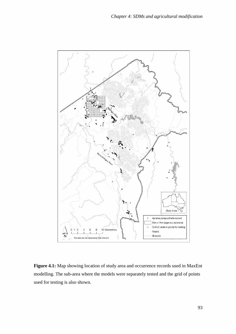
Chapter 4: SDMs and agricultural modification
93
Figure 4.1: Map showing location of study area and occurrence records used in MaxEnt
modelling. The sub-area where the models were separately tested and the grid of points
used for testing is also shown.
Chapter 4: SDMs and agricultural modification
94
Selection of modelling package
I selected the presence only MaxEnt package (Phillips et al. 2004) for the
modelling. This choice was made because there has not yet been a systematic survey of
the whole study area. Therefore, presence/absence methods are not appropriate (Elith et
al. 2011). MaxEnt is widely used and known to be one of the best performing SDM
packages (Elith et al. 2006; Hernandez et al. 2006). There have been some concerns
raised about MaxEnt providing a suitability index rather than probability of occurrence
estimates (Royle et al. 2012). However, as This study is concerned primarily with
characterising the contribution of agricultural modification, I considered MaxEnt to be a
suitable package. In addition, the habitat mapping allowed for evaluation of the
performance of the model predictions and optimisation of the threshold of the model.
Data layer selection
Environmental layers and presence data for A. parapulchella were obtained from
the Australian Capital Territory Government Conservation Research and Planning unit.
This data included wildlife atlas records as well as records from other surveys (Jones
1992; Jones 1999; Osborne and Coghlan 2004; Osborne and McKergow 1993). These
data were supplemented considerably with data (258 records) collected using GPS
during extensive surveys conducted within the study area (Osborne and Wong 2010; D.
Wong unpublished data; Wong and Osborne 2010). The accuracy of the data is likely to
have varied, with records collected before the advent of GPS more likely to be subject
to positional error. However, the data were checked for plausibility and records that
appeared likely to be erroneous were excluded. The initial set of environmental layers
consisted of topographical layers derived from a 25m digital elevation model (DEM) of
the Australian Capital Territory region and climatic layers for mean monthly maximum
Chapter 4: SDMs and agricultural modification
95
and minimum temperature and mean monthly rainfall calculated using ESOCLIM
(Houlder et al. 2000). This application derives climatic surfaces based on climate data
and a DEM. Solar radiation was derived in ArcGIS 9.3.1 (ESRI 1999 - 2009) using the
25m DEM.
Environmental layers were selected based on what were considered to be the
most ecologically relevant for the species (sensu Austin 2002) Variables that were very
highly inter-correlated [r > 0.75] (Appendix 3) were removed. Whilst MaxEnt
incorporates L1 regularization, that is known to perform well in feature selection
(Hastie et al. 2009) some level of variable pre-selection (i.e. using ecologically relevant
variables) is considered prudent (Elith et al. 2011).
Previous studies have shown that A parapulchella is unlikely to be found in
areas that have undergone very high levels of agricultural modification (Jones 1999;
Osborne and McKergow 1993). Therefore, I included agricultural modification in the
model. Native summer growing grasses are known to be gradually replaced by exotic
winter growing species as levels of grazing and fertiliser addition increase in mesic
areas (Groves et al. 2003; Stuwe and Parsons 1977). Therefore, for the agricultural
modification variable, I used a vegetation classification provided by the New South
Wales Office of Environment and Heritage (Environmental Research and Information
Consortium 2001). This classification used the differences in spectral reflectance
between remotely sensed images in spring and summer to discriminate between areas
dominated by C4 (primarily summer growing native) and C3 (primarily winter growing
exotic) grasses and was based on the methods developed by Langston (1996). The
classification had been verified in the field and since refined based on known sites in
New South Wales (Environmental Research and Information Consortium 2001, R.
Chapter 4: SDMs and agricultural modification
96
Rehwinkel, NSW Office of Environment and Heritage pers. comm.). I reclassified the
original classification of 23 classes into four classes: native grassy areas (C4
dominated), woodland, exotic (or degraded native) grassy areas and unknown. Some
areas of the extent (forested areas of > 30 % tree cover, and urban area) had been
masked out when the original classification was produced, but since there are no records
of the species from forested sites in the Australian Capital Territory or surrounds
(except for one site at Black Mountain which is located in an open area within open
forest), this was not considered to be a limitation.
Relationships between A. parapulchella and the environmental variables
geology, slope, aspect, solar radiation and soil type have all been previously described
(Jones 1999; Osborne et al. 1991) Therefore, these variables included in the model.
Solar radiation was included in the initial model but was subsequently dropped because
it made little contribution. Elevation was highly correlated with temperature. Because
variables with a direct physiological effect on species distribution are preferable to
indirect variables (Austin 2002), I excluded elevation from the analysis in favour of
temperature. A. parapulchella is thought to disperse and breed and in spring (Jones
1999); so, I included mean minimum temperature in October and mean monthly rainfall
in October in the model. Minimum temperature was selected over maximum
temperature because low temperatures are more limiting to reptiles than high
temperatures (Heatwole and Taylor 1987).
Environmental layers were prepared in ArcGIS 9.3.1 (ESRI 1999 - 2009). Raster
files were converted to ASCII data layers with a cell size of 25m in GDA 1994 Zone 55
MGA projection (Koy 2009).
Chapter 4: SDMs and agricultural modification
97
Modelling and optimisation
In order to reduce the likelihood of sampling bias affecting the final model, I
removed records that were spatially located less than 30m from another record. I ran
the model with 50% of the records (168 records) allocated for model training and the
remaining 50% selected randomly by MaxEnt for testing. Ten replicates of the model
were run and the average of these models used in the analysis.
Field Mapping
Detailed mapping of potential habitat for A. parapulchella was undertaken in
parts of the study area. This was achieved by firstly digitising areas of rocky habitat in a
GIS using a fine resolution (10cm resolution) orthophotograph layer provided by the
Australian Capital Territory Government. The boundaries of habitat were then refined
through field inspection and each habitat patch was classed as being of high, moderate
or low habitat quality based on the vegetation present. Areas containing suitable rocky
habitat that contained vegetation characteristic of low levels of disturbance (dominated
by native large tussock species [e.g. Aristida ramosa, Cymbopogon refractus, Dianella
spp., Lomandra spp., Poa sieberiana, Sorghum leiocladum or Themeda triandra.]
(McIntyre and Tongway 2005) or with a diverse range of disturbance sensitive species
[see Apendix 1 contained within Appendix 5 of this thesis for a list containing
disturbance sensitive species found within grassy ecosystems]) were classed as high
quality potential habitat. Areas containing suitable rocky habitat dominated by more
disturbance-tolerant native grasses such as Austrodanthonia spp. and Austrostipa spp.
and containing little or no occurrence of disturbance sensitive forb species were classed
as moderate quality potential habitat. Areas containing suitable rock but with very little
Chapter 4: SDMs and agricultural modification
98
or no evidence of native grass species (or areas that had undergone extreme levels of
disturbance [e.g. plantation forestry]) were classed as low quality potential habitat.
Testing the effect of agricultural modification
To test the importance of including agricultural modification data, I ran a model
with the same settings but excluded the agricultural modification layer. I compared the
area under the receiver operating curve [AUC] (Hanley and NcNeil 1982; Pearce and
Ferrier 2000) and gain (Phillips 2006) values calculated by MaxEnt for models with and
without the agricultural modification layer. The gain is a measure of the improvement in
penalized average log likelihood compared to a null model (Elith et al. 2011). Higher
values of AUC and gain indicated better model performance.
I also compared the outputs of predicted presence and absence using the
threshold suggested by MaxEnt that maximised implied specificity (i.e. the threshold
with the smallest fractional predicted area [equal training sensitivity and specificity;
threshold = 0.32 for model with agricultural modification included and 0.341 for the
model that did not include the agricultural variable]). The threshold which maximised
implied specificity was chosen as signs of over-prediction were detected during
exploratory analysis. I compared the area of predicted habitat with and without
agricultural modification according to vegetation class and generated a difference plot
based on these results.
As another way of comparing model performance, I took a subsample of the
records from the 6 x 7 km sub-area within the greater study area. Predicted probability
of presence values corresponding with the 74 presence records in the sub-area were
extracted for each model and a Welch two sample t-test was conducted to determine if
Chapter 4: SDMs and agricultural modification
99
the sample means differed significantly. The process was then repeated for a regular
grid of points generated at 500m intervals across the same sub-area. Points in this grid
that coincided with areas classified in the field as potential habitat for A. parapulchella
were excluded in order to bias this grid of points towards sites likely to be absent. This
resulted in a total of 133 points. A higher average probability of presence at recorded
presence locations should indicate that the model performs better in terms of sensitivity
(i.e. lower the likelihood of omission) and a lower average probability of presence for
the regular grid of points should indicate that the model performs better in terms of
specificity (i.e. lower likelihood of commission). Confusion matrices (Fielding and Bell
2002) were generated for models of predicted presence with and without agricultural
modification using the threshold suggested by MaxEnt that maximised implied
specificity (equal training sensitivity and specificity [threshold = 0.32 for model with
agricultural modification variable and threshold = 0.341 for model without agricultural
modification variable]) and an arbitrary threshold of 0.5 to determine the cut-off for
presence. A confusion matrix is a 2 x 2 table which shows the number of points where a
model correctly and incorrectly predicts known presence and absence points. From
these confusion matrices, I calculated the overall performance (correct classification
rate), omission rate (proportion of known presences predicted as absent) and
commission index [proportion of points from the regular grid predicted as presences]
(Anderson et al. 2003; Fielding and Bell 2002). For these values, a higher overall
performance value indicates more points are being correctly classified. A lower
omission rate indicates better sensitivity of the model (or a higher proportion of true
positive predicted) and a lower commission index indicates higher model specificity or
a lower probability that the model will predict false positives. For presence-only
Chapter 4: SDMs and agricultural modification
100
models, this index includes genuine false positives as well as points from the regular
grid that fall on suitable habitat that has not yet been identified. This is the reason for
terming this value an index rather than a rate (Anderson et al. 2003).
The models were also assessed visually, based on expert knowledge, against
detailed field mapping that was carried out in an area close to the 6 x 7 km sub-area to
determine how well the models predicted Pink-tailed Worm-lizard habitat. I compared
mapped habitat with predicted presence from models with and without the agricultural
modification variable using the threshold suggested by MaxEnt and an arbitrary
threshold of 0.5. Since using a threshold of 0.5 appeared to approximate well the areas
of known optimal habitat in the area that had been mapped, I compared the outputs with
and without agricultural modification using a threshold of 0.5 as the cut-off for presence
in order to give an indication of how much habitat had declined from optimal habitat in
the sub-area and across the greater study area. This was done by using the difference
map (calculated in ArcGIS to show areas of difference in the models by vegetation
class) and calculating the percentage of the predicted presence pixels (of the total
presence pixels for the study area) in the “exotic or degraded native” vegetation class as
well as “exotic or degraded native” + “unknown” vegetation classes identified by the
model without agricultural modification but not by the model with agricultural
modification. This resulted in a range of figures for habitat decline that took into
account the possibility of the unknown habitat being exotic (as the proximity of
unknown pixels to exotic pixels suggested this may be the case).
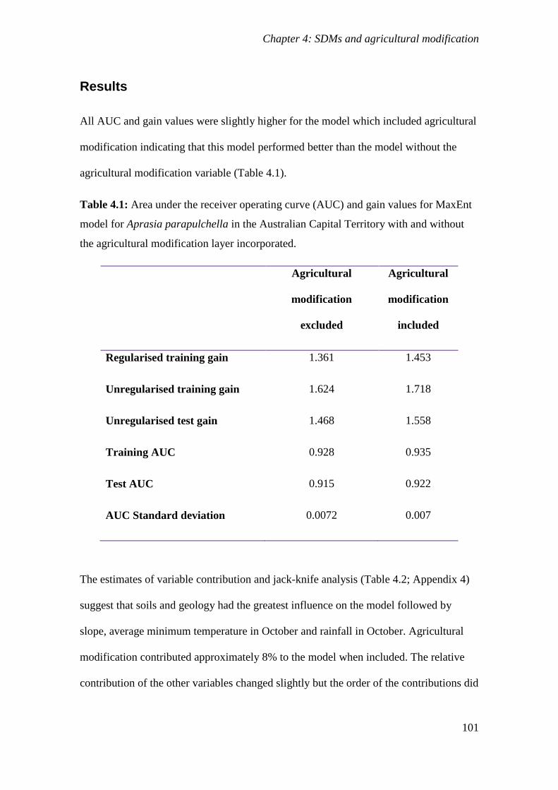
Chapter 4: SDMs and agricultural modification
101
Results
All AUC and gain values were slightly higher for the model which included agricultural
modification indicating that this model performed better than the model without the
agricultural modification variable (Table 4.1).
Table 4.1: Area under the receiver operating curve (AUC) and gain values for MaxEnt
model for Aprasia parapulchella in the Australian Capital Territory with and without
the agricultural modification layer incorporated.
Agricultural
modification
excluded
Agricultural
modification
included
Regularised training gain 1.361 1.453
Unregularised training gain 1.624 1.718
Unregularised test gain 1.468 1.558
Training AUC 0.928 0.935
Test AUC 0.915 0.922
AUC Standard deviation 0.0072 0.007
The estimates of variable contribution and jack-knife analysis (Table 4.2; Appendix 4)
suggest that soils and geology had the greatest influence on the model followed by
slope, average minimum temperature in October and rainfall in October. Agricultural
modification contributed approximately 8% to the model when included. The relative
contribution of the other variables changed slightly but the order of the contributions did
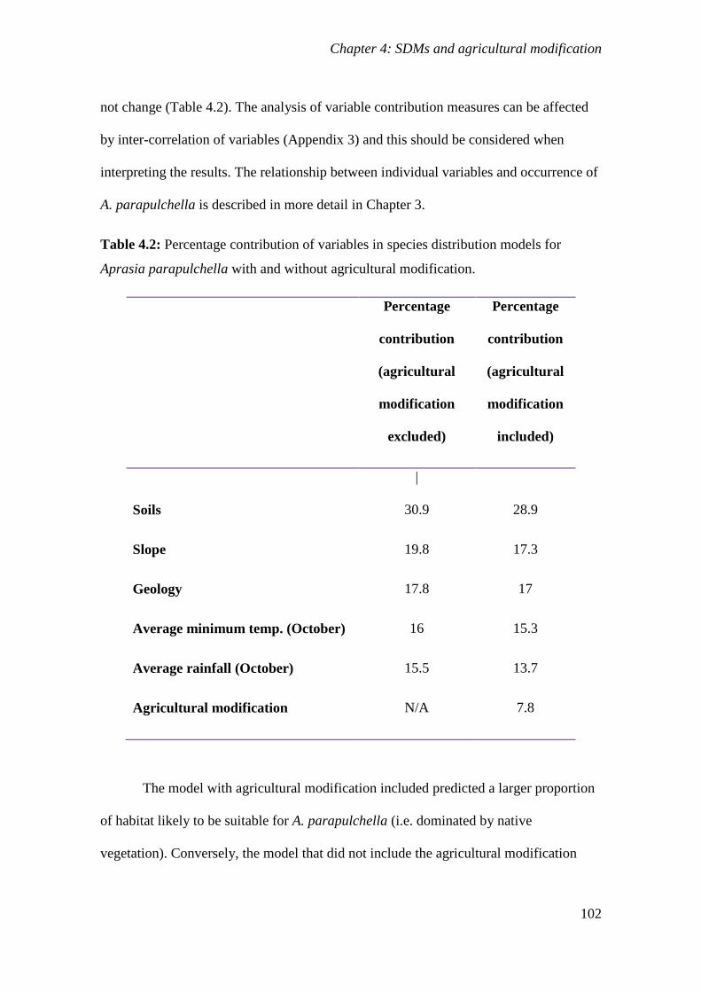
Chapter 4: SDMs and agricultural modification
102
not change (Table 4.2). The analysis of variable contribution measures can be affected
by inter-correlation of variables (Appendix 3) and this should be considered when
interpreting the results. The relationship between individual variables and occurrence of
A. parapulchella is described in more detail in Chapter 3.
Table 4.2: Percentage contribution of variables in species distribution models for
Aprasia parapulchella with and without agricultural modification.
Percentage
contribution
(agricultural
modification
excluded)
Percentage
contribution
(agricultural
modification
included)
Soils
|
30.9
28.9
Slope 19.8 17.3
Geology 17.8 17
Average minimum temp. (October) 16 15.3
Average rainfall (October) 15.5 13.7
Agricultural modification N/A 7.8
The model with agricultural modification included predicted a larger proportion
of habitat likely to be suitable for A. parapulchella (i.e. dominated by native
vegetation). Conversely, the model that did not include the agricultural modification
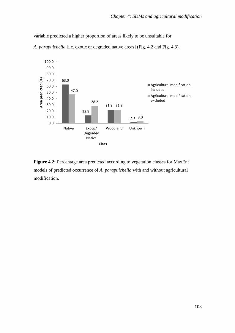
Chapter 4: SDMs and agricultural modification
103
variable predicted a higher proportion of areas likely to be unsuitable for
A. parapulchella [i.e. exotic or degraded native areas] (Fig. 4.2 and Fig. 4.3).
Figure 4.2: Percentage area predicted according to vegetation classes for MaxEnt
models of predicted occurrence of A. parapulchella with and without agricultural
modification.
63.0
12.8
21.9
2.3
47.0
28.2 21.8
3.0
0.0
10.0
20.0
30.0
40.0
50.0
60.0
70.0
80.0
90.0
100.0
Native Exotic/Degraded
Native
Woodland Unknown
Are
a p
red
icte
d (
%)
Class
Agricultural modificationincluded
Agricultural modificationexcluded
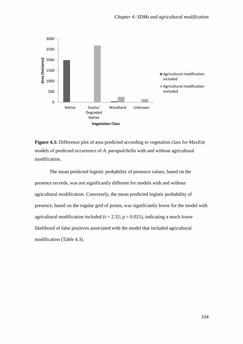
Chapter 4: SDMs and agricultural modification
104
Figure 4.3: Difference plot of area predicted according to vegetation class for MaxEnt
models of predicted occurrence of A. parapulchella with and without agricultural
modification.
The mean predicted logistic probability of presence values, based on the
presence records, was not significantly different for models with and without
agricultural modification. Conversely, the mean predicted logistic probability of
presence, based on the regular grid of points, was significantly lower for the model with
agricultural modification included (t = 2.32; p = 0.021), indicating a much lower
likelihood of false positives associated with the model that included agricultural
modification (Table 4.3).
0
500
1000
1500
2000
2500
3000
Native Exotic/Degraded
Native
Woodland Unknown
Are
a (h
ect
are
s)
Vegetation Class
Agricultural modificationincluded
Agricultural modificationexcluded
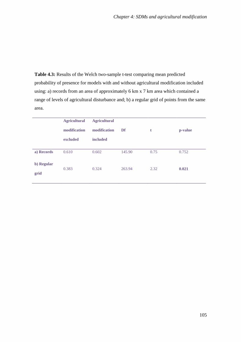
Chapter 4: SDMs and agricultural modification
105
Table 4.3: Results of the Welch two-sample t-test comparing mean predicted
probability of presence for models with and without agricultural modification included
using: a) records from an area of approximately 6 km x 7 km area which contained a
range of levels of agricultural disturbance and; b) a regular grid of points from the same
area.
Agricultural
modification
excluded
Agricultural
modification
included
Df t p-value
a) Records 0.610 0.602 145.90 0.75 0.752
b) Regular
grid
0.383 0.324 263.94 2.32 0.021
Chapter 4: SDMs and agricultural modification
106
Examination of the values derived from confusion matrices for models with and
without agricultural modification using the threshold suggested by MaxEnt and an
arbitrary threshold of 0.5 (Table 4.4), indicated that, whilst the omission rate was
slightly lower for models without agricultural modification, the commission index was
markedly higher. As a result, correct classification rates were higher for models with
agricultural modification. When a threshold of 0.5 was applied to the model the
omission rate increased, but the commission index decreased, particularly in the model
with agricultural modification, leading to an increased correct classification rate. For the
threshold of 0.5, the total area predicted by the model with agricultural modification
was 71.7% of that predicted by the model without agricultural modification (Table 4.4).
Analysis of the difference map revealed that areas classed as exotic and predicted as
suitable by the model without agricultural modification, but not by the model with
agricultural modification accounted for 31.5% of the sub-area. This figure increased to
35.2% when both the exotic and unknown classes were considered together. When the
calculation was applied across the greater study area, the corresponding values were
21% (exotic) to 22.3% (exotic + unknown).
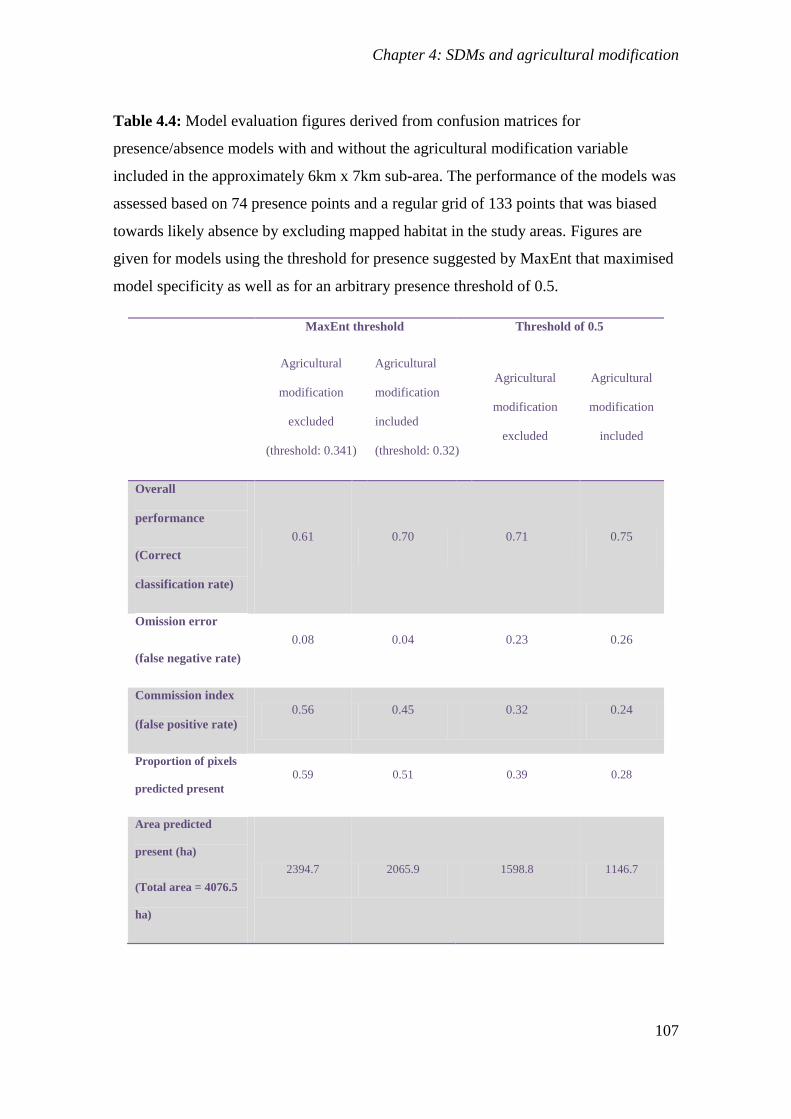
Chapter 4: SDMs and agricultural modification
107
Table 4.4: Model evaluation figures derived from confusion matrices for
presence/absence models with and without the agricultural modification variable
included in the approximately 6km x 7km sub-area. The performance of the models was
assessed based on 74 presence points and a regular grid of 133 points that was biased
towards likely absence by excluding mapped habitat in the study areas. Figures are
given for models using the threshold for presence suggested by MaxEnt that maximised
model specificity as well as for an arbitrary presence threshold of 0.5.
MaxEnt threshold Threshold of 0.5
Agricultural
modification
excluded
(threshold: 0.341)
Agricultural
modification
included
(threshold: 0.32)
Agricultural
modification
excluded
Agricultural
modification
included
Overall
performance
(Correct
classification rate)
0.61 0.70 0.71 0.75
Omission error
(false negative rate)
0.08 0.04 0.23 0.26
Commission index
(false positive rate)
0.56 0.45 0.32 0.24
Proportion of pixels
predicted present
0.59 0.51 0.39 0.28
Area predicted
present (ha)
(Total area = 4076.5
ha)
2394.7 2065.9 1598.8 1146.7
Chapter 4: SDMs and agricultural modification
108
Expert inspection of the models with and without agricultural modification
incorporated against habitat, mapped in the field (Fig. 4.4), revealed that the model with
agricultural modification provided a better characterisation of potential habitat mapped
by experts in the field than the model without agricultural modification. The presence
threshold suggested by MaxEnt led to models which over-predicted suitable habitat
whether agricultural modification was included or not. The arbitrary threshold of 0.5 led
to predictions very close to the mapped habitat areas for the model with agricultural
modification. By contrast, the changes to the model without agricultural modification
were slight when a threshold of 0.5 was used (Fig. 4.4). It should be noted however, that
using a threshold of 0.5 led to a predicted presence model that under-predicted
occurrence for areas where records were sparser (e.g. parts of New South Wales).
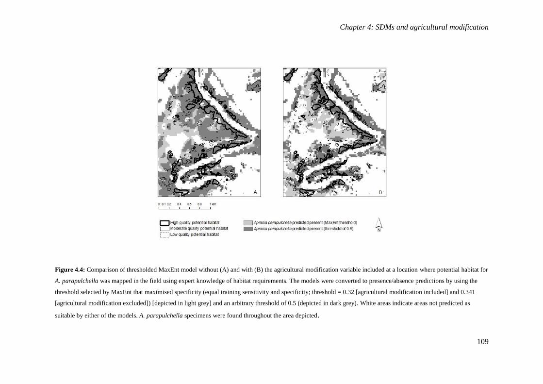
Chapter 4: SDMs and agricultural modification
109
Figure 4.4: Comparison of thresholded MaxEnt model without (A) and with (B) the agricultural modification variable included at a location where potential habitat for
A. parapulchella was mapped in the field using expert knowledge of habitat requirements. The models were converted to presence/absence predictions by using the
threshold selected by MaxEnt that maximised specificity (equal training sensitivity and specificity; threshold = 0.32 [agricultural modification included] and 0.341
[agricultural modification excluded]) [depicted in light grey] and an arbitrary threshold of 0.5 (depicted in dark grey). White areas indicate areas not predicted as
suitable by either of the models. A. parapulchella specimens were found throughout the area depicted.
Chapter 4: SDMs and agricultural modification
110
Discussion
The results demonstrated that incorporating agricultural modification as a factor
within a species distribution modelling framework clearly improved the SDM for the
threatened, habitat specialist Pink-tailed Worm-lizard, A. parapulchella. This finding
strengthens the argument that agricultural modification such as intensive grazing and pasture
improvement are likely to have led to a degradation or loss of A. parapulchella across its
range (Jones 1999; Langston 1996). Although the percentage contribution of the agricultural
modification variable was lower than the contribution of other variables and the increase in
AUC value was small (Table 4.1), this may be due to the fact that variables that act on a
broader spatial scale, such as climate, geology and topography, are likely to be the most
influential variables over the whole study area, whilst disturbance is important at finer scales
(Mackey and Lindenmayer 2001). Therefore, the changes to the model as a result of adding
agricultural modification as a factor are likely to be in the form of refinements at the local
scale rather than major changes to the model. Nonetheless, the analyses showed that the
improvement to model specificity was marked at the local scale (Table 4.3; Table 4.4;
Fig. 4.3). Such models are therefore likely to be of use to farmers, planners and conservation
managers as this is often the scale at which farm or reserve management is planned and
implemented.
Comparison of the models
The finding that adding the agricultural modification variable leads to significant
improvements in model specificity (Table 4.3; Table 4.4) is consistent with what might be the
expected pattern according to niche theory (Grinnell 1917; Hutchinson 1957). As agricultural
disturbance reduces the amount of suitable habitat, it reduces the size of the available
ecological niche (Hirzel and Le Lay 2008) that can be exploited. Therefore, incorporation of
Chapter 4: SDMs and agricultural modification
111
agricultural modification should allow better prediction of the extent of this ecological niche
which has been modified within approximately the last 100 years. Expert inspection of the
model outputs in conjunction with field mapping of potential habitat for A. parapulchella
showed that the model with agricultural modification included was much more effective in
identifying expert predicted habitat. However, the predicted presence-absence layer based on
the threshold suggested by MaxEnt (equal training sensitivity and sensitivity [0.317]) still
appeared to over-estimate suitable habitat and the area predicted was almost double that of the
presence/absence model that used a threshold of 0.5 (Table 4.4). This highlights a possible
limitation of MaxEnt that warrants further attention. The findings suggest that neglecting to
include agricultural modification data leads to over-prediction of suitable habitat in areas that
have undergone high levels of agricultural modification. This could lead to managers
believing that unsuitable areas are in fact suitable for the species. Interestingly, MaxEnt is
known for performing well with respect to commission errors (Elith et al. 2006; Swenson
2008). However, the prevalence of a given species may influence prediction in methods (such
as MaxEnt) which use the receiver operating curve to optimise thresholds (Manel et al. 2001).
If we assume that, using a presence threshold of 0.5, the model without agricultural
modification represents suitable areas of optimal habitat for A. parapulchella, the results of
the modelling suggest agricultural modification may have led to decline or loss of at least 30 -
35% of optimal habitat in the sub-area of study (Table 4.4). Applying this calculation across
the ACT, suggests a decline or loss of approximately 20% or more of optimal habitat across
the Australian Capital Territory. It should be noted that both models are based on modern-day
occurrence records (since 1974) and this is likely to have influenced the model. For example,
the species may be completely absent from areas in the environmental space that have
experienced long periods of intensive agricultural disturbance. Therefore, the estimates of loss
and degradation of habitat may be lower than the actual loss and degradation that has occurred.
Chapter 4: SDMs and agricultural modification
112
Whilst this possibility should be considered, the findings of this study suggest there is
potential for comparison of models with and without disturbance to identify areas where a
given species has declined as a result of disturbance as well as to monitor decline or
improvement of the habitat of species or communities.
There are clear implications of this modelling for the longer term conservation of
A. parapulchella. In the ACT, 99 year leases have recently been granted to rural landholders
in order to provide greater security of tenure (G. Hirth, ACT Parks Conservation and Lands,
pers. comm.). This presents a potential risk to the habitat and populations of A. parapulchella
located on rural land as the added security of tenure may lead to landholders intensifying
activities. It appears that fertiliser addition in particular may be a major threat to
A. parapulchella as well as to other reptile fauna within this context (Dorrough et al. 2012;
Osborne and McKergow 1993). Therefore, for conservation of A. parapulchella on rural land,
working with farmers to identify and protect suitable habitat and preserve connectivity for the
species will be essential. There is the potential for such areas to play an important role in
complementing areas with higher levels of formal protection such as reserves. Monitoring of
changes in floristics over time using remote sensing could also inform management and
identify areas where populations may be at threat. Urban development and forestry are the
other major causes for habitat loss in the ACT and further research could be undertaken to
estimate likely losses associated with each of these forms of disturbance.
The hypothesis that the nature of land tenure has influenced the current distribution of
A. parapulchella (Jones 1999) has not been explicitly examined. This question is complex and
worthy of further study. Unlike threatened reptile species which live in grasslands,
A. parapulchella occupies rocky parts of the landscape, which are therefore less conducive to
intensive use than non-rocky areas. Comparisons of the impact of agriculture on rocky areas
in New South Wales and the ACT would help to answer this important question.
Chapter 4: SDMs and agricultural modification
113
I found that the model that included agricultural modification predicted a higher area
of native grass cover (C4) and a lower area of exotic/degraded native (C3) grass cover as
occupied than the model without agricultural modification (Fig. 4.2; Fig. 4.3). Therefore, the
predictions of the model with agricultural modification included are more consistent with
findings that A. parapulchella requires areas dominated by native vegetation and cannot
persist in areas that have undergone very high levels of agricultural modification,
characterised by a cover of almost exclusively exotic grasses (Jones 1999; Osborne and
McKergow 1993). Nonetheless, some of the areas classed as exotic may, in fact, be degraded
native areas dominated by C3 species of grass (R. Rehwinkel, NSW Office Environment and
Heritage, pers. comm.). Such areas may still support A. parapulchella (Jones 1999), so this
should be considered when interpreting the model. It is likely that, with respect to
A. parapulchella, the model including agricultural disturbance will be most useful for
identifying the highest quality potential habitat for the species. These areas are likely to be the
areas of highest priority for the conservation of the species. Further refinement of the model
may be possible if spectral data can be used to identify rocky areas as the species is dependent
on areas of shallowly embedded rock in the Australian Capital Territory (Wong et al. 2011).
The results also indicate that the threshold used as a cut-off for presence is important,
and thresholds suggested by MaxEnt may over-predict suitable habitat in some situations
(Fig. 4.3). One of the possible reasons for this is that many users of modelling software such
as MaxEnt are interested in overall distributions of species and often at broad spatial scales
(Pearson and Dawson 2004). There has also been some research that indicates that using AUC
to optimise thresholds for predicted occurrence can lead to overestimation of suitable habitat
for species which have low prevalence in the landscape (Manel et al. 2001). However, the
threshold used depends on the purpose. If the goal is to find all areas where a species may
occur across the region (e.g. for impact assessment where a precautionary approach is
Chapter 4: SDMs and agricultural modification
114
desirable), a conservative threshold would be appropriate. If fine-scale prediction of high
quality suitable habitat is the goal, higher thresholds may be favoured (Pearce and Ferrier
2000). In such cases, optimisation of thresholds to minimise commission error may be
appropriate. However, for presence-only modelling, this may be a challenge if the rate of
occurrence of the species in the landscape is unknown (Anderson et al. 2003; Elith et al.
2011). Optimisation using mapped habitat is one way of addressing this problem. A similar
approach to that taken in this study could be used for optimisation in cases where suitable
habitat is readily identifiable. It is important, however, to keep the goals of the modelling
exercise in mind when conducting such optimisation. The results suggest that caution should
be taken with respect to areas where less sampling has taken place. In such areas, a more
liberal threshold (such as those suggested by MaxEnt) may be appropriate for habitat
prediction.
The findings of this study demonstrate that incorporating agricultural modification
data into a SDM reduced the likelihood of errors of commission in areas that are predicted to
have undergone agricultural modification. SDMs that include disturbance have the potential
to provide better information to farmers, planners and conservation managers to inform
conservation management plans or specific actions aimed at habitat restoration as well as to
provide information about habitat decline or loss. There is potential for future work to
investigate the contribution of agricultural modification within species distribution models for
other species and at broader spatial scales.
Acknowledgements
I thank Mike Austin of CSIRO, Andre Zerger of the Australian Bureau of Meteorology and
Margaret Kitchin of Australian Capital Territory Conservation Planning and Research for
advice regarding modelling and for providing data layers. Rainer Rehwinkel of the New
Chapter 4: SDMs and agricultural modification
115
South Wales Office of Environment and Heritage provided the remote sensing data and
helpful information regarding the agricultural modification data. Annabel Smith, Ingrid
Stirnemann, Nicole Maron, David Leigh, Percy Wong and Elisabeth Wong provided useful
comments on manuscript. Finally, I thank the Australian Capital Territory Government for
providing funding to undertake the project, data layers and specimen records. This study was
authorised by the University of Canberra Committee for Ethics in Animal Experimentation
(project authorisation code CEAE08-17).

Chapter 4: SDMs and agricultural modification
116
Chapter 5: Factors at the patch scale
117
5. Factors affecting the occurrence of a threatened legless-
lizard at the patch scale
Abstract
Agricultural modification is one of the main drivers of biodiversity decline. The Pink-tailed
Worm-lizard Aprasia parapulchella (Pygopodidae) is an example of a threatened species
which is thought to decline with agricultural modification owing to changes in habitat.
However, this relationship has not been explored in detail. I used boosted regression trees to
determine the relationship between habitat factors and abundance of A. parapulchella at the
patch scale in the Australian Capital Territory, located in south-eastern Australia. Percentage
cover of large tussock forming grasses explained 46% of the variation in the model and site
floristic score accounted for 33% of the variation. The other variables that contributed to the
model included: percentage cover of rock (10%), number of turnable rocks (5%) and relative
density of rocks occupied by ants of the size class known to occur with A. parapulchella
(5%). The results indicate that vegetation characteristics are the best predictors of the
abundance of A. parapulchella at the local scale. Management strategies that promote return
to a vegetation state similar to the original state in south-eastern Australia (i.e. dominated by
large tussock forming grass species such as Kangaroo Grass Themeda australis) are likely to
be most beneficial for providing the optimum habitat for A. parapulchella.
Chapter 5: Factors at the patch scale
118
Introduction
The impact of agricultural activities on biodiversity has received much attention in recent
years. A range of practices employed by agricultural systems such as clearing of vegetation,
tillage, grazing, fertiliser addition, pesticide use and drainage of wetlands have significant
impacts on biodiversity (McLaughlin and Mineau 1995). These practices often lead to long-
term alteration of the soil structure, changes to nutrient cycling and biogeochemical processes
(Foster et al. 2003; Richter et al. 2000), and to a loss of biodiversity or alteration in species
composition or dynamics in vegetation (Clarke 2003; Dorrough et al. 2007), reptiles (Brown
2001; Brown et al. 2008; James 2003), mammals (Kutt and Woinarski 2007) and birds (Ford
et al. 2001; James 2003).
Recent research in eastern Australia has addressed the decline of reptile biodiversity as a
result of historical and continuing agricultural disturbance (Brown 2001; Brown et al. 2008;
Brown et al. in press; James 2003; Woinarski and Ash 2002; Wong et al. 2011). In addition,
the value of rocky outcrops for reptile biodiversity within agricultural landscapes has been
identified as an important issue (Cogger et al. 1993; Michael et al. 2008; Pike et al. 2010) but
has received relatively little attention in the academic literature.
The Pink-tailed Worm-lizard Aprasia parapulchella is a habitat specialist which, at most
locations where it has been recorded, depends on the availability of suitable rocky habitat
(Jones 1999; Osborne et al. 1991). The known distribution of the species is extremely disjunct
(Wong et al. 2011) and this is thought to be a direct result of habitat loss and degradation,
largely through historical agricultural activities and their related impacts (Jones 1999;
Osborne et al. 1991). The expansion of plantation forestry and urbanisation are also important
threatening processes. Whilst the direct effects of urban development and forestry on the
habitat of A. parapulchella are often immediately apparent, the effects of agricultural
Chapter 5: Factors at the patch scale
119
practices can be more difficult to detect as there are no apparent planted trees or structures
present in the landscape. It is likely that gradual degradation or loss of the habitat of
A. parapulchella has occurred across its range through processes associated with agricultural
development such as ploughing, rock removal, pasture improvement, spread of weeds and
over-grazing by livestock. As A. parapulchella is thought to be sensitive to disturbance (Jones
1999; Osborne and McKergow 1993), analysis of the response of this species to disturbance
related to agriculture is likely to provide insights which could benefit not only
A. parapulchella but also the suite of taxa associated with rocky outcrops.
To examine the extent of the relationship between agricultural modification and the
presence and abundance of A. parapulchella, it is important to consider the particular farming
activities that are most likely to have led to population declines and extirpation from the
agricultural landscapes. Whilst it difficult to assess the effects of historical farming activities
on the current distribution of the species, it is highly likely that these practices have played an
important role in the decline of the species across its range. The possibility that the clearing of
tree cover at the time of European settlement may initially have allowed for an expansion of
populations into nearby rocky environments that previously were covered in forest [for
example parts of Canberra Nature Park in the Australian Capital Territory] (Osborne and
McKergow 1993) is acknowledged. However, intensive landscape scale agricultural practices
associated with crop production and livestock grazing (ploughing, removal of stones,
conversion of native pasture to exotic pasture) undoubtedly will have had a major influence
on the species. It is possible that such processes will have led to its disappearance from vast
areas of its former range. This view is supported by the observations that: (1) the highest
abundances of A. parapulchella are more likely to be found at sites where the vegetation
floristic composition is indicative of lower levels of agricultural modification; (2) the species
is not found at the most highly disturbed sites (Jones 1999; Osborne et al. 1991); and (3) it is
Chapter 5: Factors at the patch scale
120
more likely to be present in sites dominated by a well-developed cover of native grasses
(Jones 1999).
The expected interaction of grazing, fertiliser addition and nutrient status (Dorrough et al.
2006) makes it difficult to analyse the effects of individual factors on the occurrence and
abundance of particular species at individual sites. This difficulty is made more complicated
by the possibility of unknown land use histories or interactions between different animal and
plant species. However, quite a significant area of study has emerged examining vegetation
responses to soil nutrient status and grazing intensity in south-eastern Australia (Dorrough et
al. 2007; Dorrough et al. 2006; Dorrough and Scroggie 2008; Groves et al. 2003; McIntyre
2008; McIntyre and Tongway 2005). In general, it is agreed that increased continuous grazing
(and associated practices such as fertiliser addition) leads to a change in the dominant
vegetation species from tall perennial warm-season growing (C4) grass species such as
Kangaroo Grass (Themeda australis) to short perennial cool-season growing (C3) grasses
such as Short Wallaby Grass (Austrodanthonia carphoides) and dwarf C4 species such as
Windmill Grass (Chloris truncata). With increasing time and intensity of grazing, exotic
annual C3 species such as (Vulpia bromoides) come to dominate and further addition of
phosphorus favours species such as Barley Grass (Hordeum leporinum) (Groves et al. 2003).
Groves et al. (2003) conducted a glasshouse experiment using monocultures and mixed
species groups of native and introduced origin. They found that native grasses were all less
competitive than introduced pasture species even at the lowest nutrient levels. Moreover,
individual species showed quite specific responses to nutrient level. In terms of physiological
performance (in absence of competition), T. australis, the most productive species in
monoculture, declined steadily with increased nutrient level; Tall Tussock Grass (Poa
labillardierei) performed maximally at intermediate nutrient levels and; A. carphoides
Chapter 5: Factors at the patch scale
121
declined at high nutrient levels. Of the introduced annuals, Squirrel Tail Fescue (Vulpia
bromoides) performed best at intermediate nutrient levels but declined at higher nutrient
levels, whilst (H. leporinum) increased in performance as nutrient levels increased, reaching a
plateau at the highest nutrient levels. The two perennial exotic species, Perennial Ryegrass
(Lolium perenne) and Cocksfoot (Dactylis glomerata) performed well at all but the lowest
nutrient levels. When relative ecological performance was assessed (i.e. performance within a
multi-species group), the native species were barely able to survive at high nutrient levels,
performing optimally at low nutrient levels. The subordinate species Vulpia performed
optimally at intermediate nutrient levels while Hordeum showed an unexpected response
curve, dominating at the lowest and four highest nutrient levels but suppressed at intermediate
levels. Lolium and Dactylis dominated at intermediate levels, but were unexpectedly
outcompeted by Hordeum at the highest nutrient levels.
Dorrough and Scroggie (2008) modelled and analysed the response of 494 southern
Australian plant species to grazing and soil phosphorus concentration gradients and examined
the influence of plant origin and two stable plant traits (longevity and growth form) on these
responses. They found that plant origin and plant traits (particularly growth form) were useful
in predicting plant response. Native perennial geophytes (mainly from the families Liliaceae,
Iridaceae and Orchidaceae), ferns and shrubs were most adversely affected by both grazing
and increased soil phosphorus concentration, whilst exotic annual grasses and forbs were
most tolerant to the two disturbance parameters. The results highlight the importance of
shared evolutionary history in relation to response of plants to anthropogenic disturbance and
illustrate the devastating impacts that such disturbance can have on plant communities that
evolved in a landscape of low soil phosphorus and without ungulate grazing (Dorrough and
Scroggie 2008).
Chapter 5: Factors at the patch scale
122
Links have also been established between grasslands dominated by large tussock
forming species and good soil surface condition (McIntyre and Tongway 2005) as well as
high biodiversity (McIntyre 2005). As a result of their findings, McIntyre and Tongway
(2005) provided the management recommendation to ‘graze conservatively to maintain
dominance of large and medium tussock grasses over 60–70% of the native pastures…and a
maximum of 30% short-grazed patches in native pastures’ (McIntyre and Tongway 2005).
The use of floristics for the assessment of vegetation condition
In practice, standardised measurements have been developed to characterise sites based on
their floristic characteristics (Rehwinkel 2007; Sharp 2006). These measurements are derived
by determining the number of sensitive species that are present at a particular site and,
therefore, may be considered a surrogate for disturbance. However, it should be noted that the
measures were originally developed to assess conservation significance rather than
disturbance. The floristic value score method (Rehwinkel 2007; Appendix 5) is used
extensively in the Southern Tabelands of south-eastern Australia to assess the floristic “value”
of a site and for planning purposes to determine whether sites fall within politically-defined
boundaries as endangered ecological communities (Rehwinkel 2007; G. Baines, pers. comm.).
Impacts of agricultural disturbance on A. parapulchella
The relationship between agricultural disturbance and the presence and abundance of
A. parapulchella has been investigated to some extent by Jones (1999) through the use of a
number of indicators of disturbance based on floristic attributes. No clear relationship was
found between the amount of disturbance and the presence of A. parapulchella. However, the
species was absent from the most highly modified sites that were dominated by exotic
species. Differences between sites where A. parapulchella were absent and those where it
occurred at the highest abundances indicated that the species occurs at highest densities at
Chapter 5: Factors at the patch scale
123
sites where native plant species were dominant. Jones (1999) found that the indicators of
disturbance that were most useful in discrimination were native plant species richness and
ratio of exotic plant species cover to native plant species cover. The proportion of rosette
herbs (often weed species) was also found to be higher at sites where A. parapulchella was
not found. Large tussock grass species (often associated with lower levels of disturbance)
(McIntyre and Tongway 2005) were found to be associated with sites where the species was
present. A. parapulchella was also found to be present at sites with higher abundance of
Vulpia bromoides, Aira elegantissima, Avena fatua and Bothriochloa macra and was less
likely to occur in association with Acaena ovina and Austrostipa bigeniculata. Jones (1999)
suggested that the association with these species may be more likely to be a result of the
historical land use in the areas where the species is most likely to be found (often secondary
grassland that has had a long history of livestock grazing) rather than a preference exhibited
by A. parapulchella for these particular species. Thus, the fact that most of the sites exhibited
some form of weed invasion may have clouded the relationships (Jones 1999).
The findings of Jones (1999) suggest that A. parapulchella is not able to persist after
the level of disturbance at a site reaches a certain level and that it reaches the highest
abundances at sites that display low levels of disturbance. Jones (1992; 1999) conducted most
of her work in areas within public land and did not use current agricultural land as a focus of
the study. Therefore, the question of whether the same relationships will hold when
production farmland is included is of considerable interest. Based on current knowledge
relating to vegetation responses to disturbance (Dorrough and Scroggie 2008; Groves et al.
2003), it would appear that the species is, however, able to persist at sites where the
vegetation species present indicate intermediate levels of disturbance resulting from historical
grazing and associated practices (e.g. fertiliser application). This paper further addresses the
Chapter 5: Factors at the patch scale
124
effect of agricultural modification (grazing and pasture improvement) on the abundance of
A. parapulchella.
I aimed to answer the following questions relating to the response of A. parapulchella to
the impacts of agricultural disturbance:
1. Can floristic measures be used as useful predictors for presence and/or abundance of
A. parapulchella?
2. What are the most important factors influencing the abundance of A. parapulchella?
The results will increase our understanding of the factors affecting occurrence and abundance
of this species as well as informing management efforts. It is hoped that the results will have
application to other species, especially those associated with rocky outcrops on agricultural
land.
Methods
Study area
The study area (Fig. 5.1) is located in the Australian Capital Territory (ACT). The ACT is
located in south-eastern Australia lying between approximate latitudes of 35o07’ S and 35
o55’
S and longitudes of 148o45’ E and 149
o25’ E. The area experiences mean maximum and
minimum temperatures of 20.0oC and 7.1
oC respectively. July is the coldest month, with an
average maximum temperature of 11.5oC and January the hottest, with an average maximum
of 28.5oC. The ACT receives a mean annual rainfall of 632.6mm. The highest rainfall occurs
in spring with September receiving the highest monthly rainfall (65.2mm). June is the driest
month, receiving on average 37.9mm of rainfall (Australian Government Bureau of
Meteorology 2010).
Chapter 5: Factors at the patch scale
125
Study sites
The 29 study sites (Fig. 5.1) were located across eight sampling locations that include areas
on leasehold farm land and in reserves on the lower lying hills within the Murrumbidgee and
Molonglo River Corridor of the ACT. The original vegetation is likely to have been largely
Yellow Box (Eucalyptus melliodora) – Blakely’s Red Gum (Eucalyptus blakelyi) grassy
woodland. However, much of the area has been cleared or partially cleared for agricultural
purposes. Some low-lying areas are considered to have been naturally without tree cover
(natural temperate grassland). Ground layer vegetation varies from sites dominated by
disturbance intolerant species such as T. australis and a range of disturbance sensitive forb
species to sites dominated by more disturbance tolerant perennial grasses such as Austrostipa
spp. and Austrodanthonia spp., to agronomic species which are able to persist in highly
modified sites such as Barley Grass Hordeum spp. It is likely that the ground layer vegetation
has been significantly altered in many sites and that all sites have been modified to some
degree due to human interaction with the landscape at some time in the past.
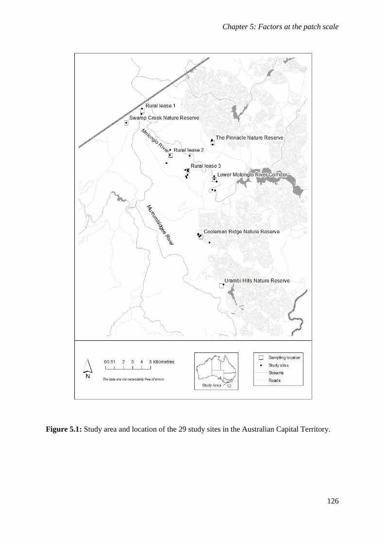
Chapter 5: Factors at the patch scale
126
Figure 5.1: Study area and location of the 29 study sites in the Australian Capital Territory.
Chapter 5: Factors at the patch scale
127
Field methods
Constrained area searches
At each of the 29 sites, an area constrained survey, based on the methods used by Jones
(1999), was undertaken in order to ascertain whether A. parapulchella was present. Jones
used area constrained searches by dividing hillsides into search lanes which were
systematically searched. Searches were undertaken in three 10m x 10m quadrats or one 10m x
30m quadrat in the current study. Where habitat was continuous, 10m x 30m quadrats were
searched; however, some outcrops were relatively small, and at these sites three separate 10m
x 10m quadrats of similar landscape and vegetation character were searched. Some sites based
on single 10m x 10m quadrats were included in the analysis. In order to supplement the
number of rocks searched at these sites, nearby areas were searched in some cases. If less than
750 rocks were turned within the three quadrats without the capture of at least one specimen
or observation of a sloughed skin, searching was continued at the site in the areas adjacent to
the quadrats until either a specimen was recorded or 750 rocks had been turned. If no
specimens or skins were uncovered within the 750 rocks, A. parapulchella was assumed to be
absent from the site or occurring at very low densities. The figure of 750 rocks is based on the
figure derived by Jones (1999) that is the number of rocks required to be turned in order to be
95% confident that the species is absent from the site when not detected (in the appropriate
time of year for searching). This value is likely to underestimate the effort required to detect
the species if it occurs at extremely low densities or if searches are undertaken outside the
optimal search period (usually between approximately the middle of August and the middle of
October in the ACT). For the purposes of the analysis, non-detection was considered to be the
same as an absence. This is a limitation of the study. However, the setting of a limit of 750
stones was seen as necessary for logistical reasons. Count data was recorded and a figure of
relative density was calculated by dividing the number of rocks occupied by one or more
Chapter 5: Factors at the patch scale
128
A. parapulchella specimens by the number of rocks turned. This figure was then multiplied by
1000 to derive a figure of relative density of occupied rocks per 1000 rocks.
Measurement of habitat attributes
At each of the 29 sites, all herbaceous species within a 10m x 10m quadrat were identified
and their percentage cover estimated visually. A 10m x 10m quadrat was chosen in preference
to a 20m x 20m quadrat as the habitat of the species is such that it consists of long linear strips
of habitat or groups of small patches of rocky habitat with dimensions smaller than 20m x
20m. A floristic value score was calculated according to the methods of Rehwinkel (2007; see
Appendix 5). For this method, floristic value is derived from the number of” sensitive”
species located in the plot over a specified cover-abundance (species with a very low cover-
abundance [1 to 3 individuals] are not included in the analysis). The cover of thick-tussock
forming grasses was then calculated. This figure was calculated by summing the percentage
cover of T australis as well as other grasses classed as being “large-tussock forming” species
(McIntyre and Tongway 2005) such as Purple Wiregrass Aristida ramosa, Barbed-wire Grass
Cymbopogon refractus and Poa Tussock Poa sieberiana, Wild Sorghum Sorghum leiocladum.
Two non-grass groups (Lomandra spp. and Dianella spp.) were also included based on their
similar (to other large tussock species) response to grazing and morphology (McIntyre and
Tongway 2005). For each 10m x10m quadrat, percentage cover of vegetation, litter, rocks,
bare ground litter and cryptogams was visually estimated.
In order to estimate home site availability, turnable rocks with an axis longer than 50mm,
were counted within the 10m x 10m quadrat. The number of rocks occupied by ants with
body lengths of 7mm or smaller was also recorded. Ants that are this size correspond with the
size of Rhytidoponera metallica, the largest sized ant commonly found to co-occur with
A. parapulchella (Jones 1999). Raw data are included in Appendix 6.
Chapter 5: Factors at the patch scale
129
Analysis
All analyses were performed in the statistical program, R version 2.14.1 (R Development
Core Team 2005). Boosted regression tree analysis was performed using the package gbm
version 1.6 – 3.1 (Ridgeway 2006) extended functions gbm step version 2.9 developed by
Jane Elith and John Leathwick .(Elith et al. 2008; supplementary material).
Disturbance indicators
In order to determine which vegetation indicators of disturbance were most closely associated
with abundance of A. parapulchella, I performed correlation analysis on the variables floristic
value score, percentage cover of T. australis and percentage cover of native grasses from the
large tussock functional group (McIntyre and Tongway 2005). Although it is a large tussock
species, percentage cover of T. australis was included separately in the analysis because of its
reported association with the lizards (Jones 1999; Osborne et al. 1991; Osborne and
McKergow 1993).
Modelling response of density of A. parapulchella to habitat variables
Exploratory analyses (after Zuur et al. 2009) revealed inter-correlation between some of the
variables (Appendix 7). For this reason, and owing to the complex nature of the ecology of
the study species, I decided to analyse the data using boosted regression trees (BRT). BRT
combines the advantages of regression trees [models that relate a response to a set of
predictors through recursive binary splits] and boosting [an adaptive method used to combine
many simple models with the result of improving predictive performance] (Elith et al. 2008).
The BRT method is highly flexible and is well suited to ecological applications. Unlike many
of the traditional statistical techniques, boosted regression tree analysis does not require
elimination of outliers or transformation of the data, allows for modelling of non-linear
relationships and is robust to complex interactions between variables (Elith et al. 2008). BRT
Chapter 5: Factors at the patch scale
130
uses boosting to avoid the problem of relying on a single tree for prediction. Boosting is a
way of minimizing a loss function, representing loss of predictive performance (e.g.
deviance), by adding a new tree at each step that best reduces the loss function (Elith et al.
2008). In the case of BRT, the first tree selected is the one that reduces the loss function the
most and subsequent trees the remaining variation not explained by the first tree.
I initially built a beyond optimal model using all explanatory variables as described in Zuur et
al. (2009). I then reduced the candidate set of variables by eliminating those with negligible
effect (Elith et al. 2008). BRT models largely ignore non-informative predictors when fitting
trees; however, variable reduction may be appropriate when sample size is small as redundant
predictors may degrade predictive ability (Elith et al. 2008). The final model used data from
29 sites using tree complexity of 3, a learning rate of 0.001 and a bag fraction of 0.9 (see Elith
et al. 2008 for a detailed explanation of these terms). The response variable used was number
of specimens of A. parapulchella recorded and the predictor variables used were: percentage
cover of large tussock species, site floristic value score, percentage cover of rocks, number of
turnable rocks per 100m2 and relative density of rocks occupied by ants colonies.
Chapter 5: Factors at the patch scale
131
Results
The summary statistics for the model are reported in Table 5.1. The percentage cover of large
tussock grasses accounted for nearly half (Fig. 5.2) of the total deviance explained by the
model, whilst ‘floristic value score’ accounted for approximately one third (Fig. 5.2) of the
total explained deviance. A three-dimensional plot of the relationship between the two
variables that contributed most to the model is shown in Figure 5.3. The remaining variables
made relatively minor contributions to the model, with percentage cover of rock accounting
for 10.9 % of the explained variation and home site availability (no. of rocks / 100m2) and
proportion of rocks occupied by ants each explaining 5.1% of the variation. Abundance of
A. parapulchella increased with cover of ‘large tussock’ species up to 10% cover at which
point the response reached a plateau. There appeared to be a threshold relationship between
A. parapulchella abundance and ‘site floristic score’. Sites with a ‘site floristic score’ of four
or greater were associated with higher abundances of A. parapulchella. Conversely,
abundance of A. parapulchella showed slightly negative threshold response at sites with a
higher percentage cover of rock, with the threshold at between 30% and 35% rock cover.
Abundance of A. parapulchella showed a marginally positive response to the number of
available home sites (turnable rocks) at a site. There was a marginally negative relationship
between the proportions of rocks occupied by ants at a site and A. parapulchella abundance.
The relationship indicated that sites with high abundances of A. parapulchella contained
lower abundances of ants.
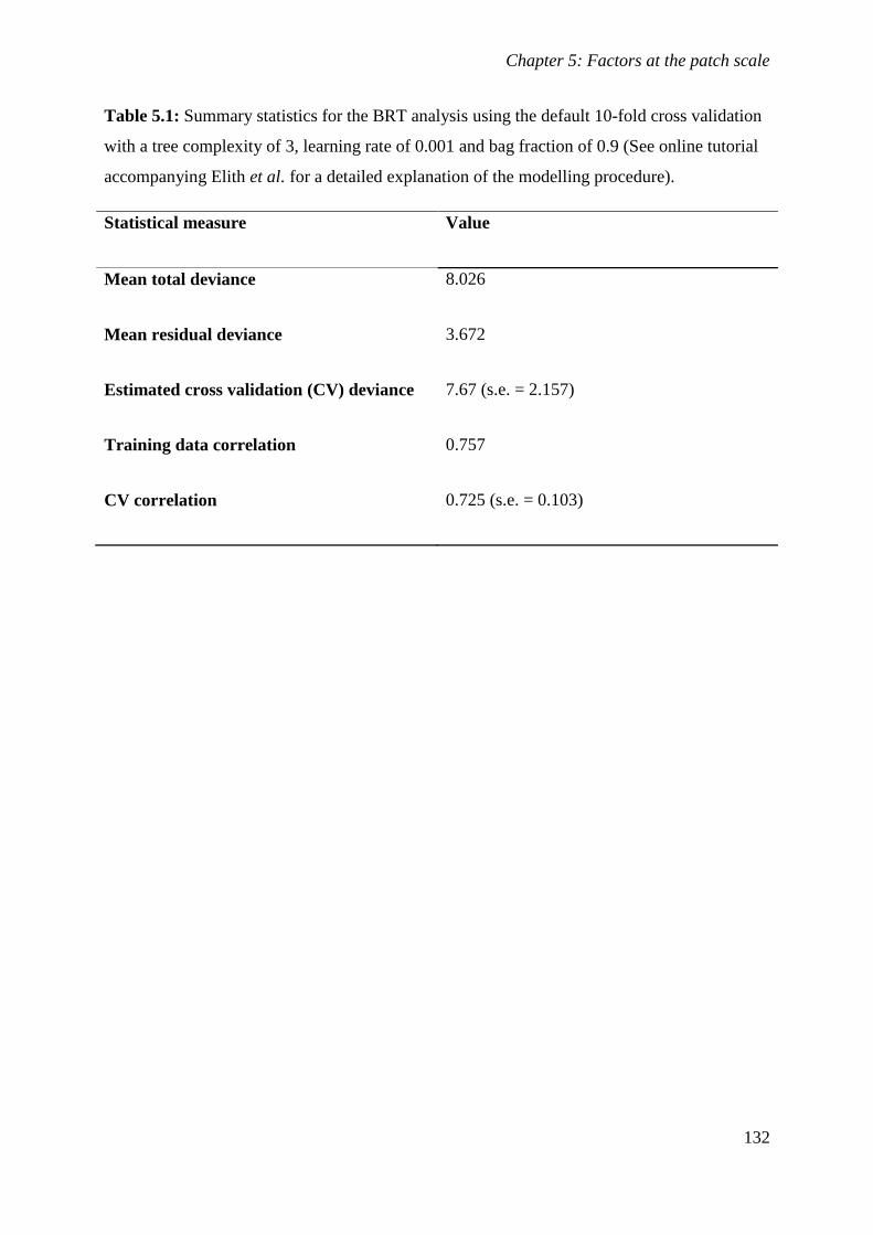
Chapter 5: Factors at the patch scale
132
Table 5.1: Summary statistics for the BRT analysis using the default 10-fold cross validation
with a tree complexity of 3, learning rate of 0.001 and bag fraction of 0.9 (See online tutorial
accompanying Elith et al. for a detailed explanation of the modelling procedure).
Statistical measure Value
Mean total deviance 8.026
Mean residual deviance 3.672
Estimated cross validation (CV) deviance 7.67 (s.e. = 2.157)
Training data correlation 0.757
CV correlation 0.725 (s.e. = 0.103)
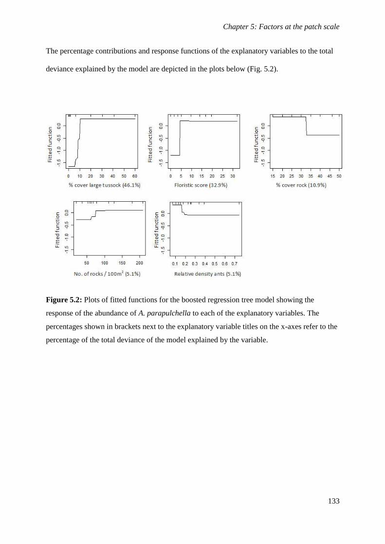
Chapter 5: Factors at the patch scale
133
The percentage contributions and response functions of the explanatory variables to the total
deviance explained by the model are depicted in the plots below (Fig. 5.2).
Figure 5.2: Plots of fitted functions for the boosted regression tree model showing the
response of the abundance of A. parapulchella to each of the explanatory variables. The
percentages shown in brackets next to the explanatory variable titles on the x-axes refer to the
percentage of the total deviance of the model explained by the variable.
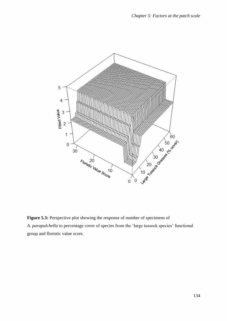
Chapter 5: Factors at the patch scale
134
Figure 5.3: Perspective plot showing the response of number of specimens of
A. parapulchella to percentage cover of species from the ‘large tussock species’ functional
group and floristic value score.
Chapter 5: Factors at the patch scale
135
Discussion
The results demonstrate the importance of the effect of changes to vegetation composition as
a result of agricultural practices such as pasture improvement and overgrazing on
A. parapulchella populations. By far the most variation in the model was explained by the
variables percentage cover of large tussock species and floristic value score. Both of these
variables are indicators of the level of historical agricultural disturbance. Of these two
variables, the abundance of A. parapulchella was most closely associated with percentage
cover of large tussock species. Percentage cover of T. australis was not found to contribute to
the model, suggesting that the prevailing view that A. parapulchella is associated with T.
australis should be reconsidered. Although it is true that a high abundance of
A. parapulchella at a site is often associated with sites where T. australis is present, it is likely
that the effect simply reflects the extent of disturbance from agricultural modification. The
results indicate that sites with higher abundances of A. parapulchella are associated with a
higher percentage cover of plants from the large tussock forming functional group identified
by McIntyre and Tongway (2005) [e.g. T. australis, A. ramosa, P. sieberi, C. refractus,
Sorghum leiocladum, Lomandra spp. and Dianella spp.]. In this study, T. australis and
A. ramosa were the main dominant species associated with such sites. The interaction
between percentage cover of large tussock grasses and site floristic score (Fig. 5.3) suggests
that higher site floristic scores can help to characterise likely abundance of A. parapulchella at
sites where no large tussock grass species are present or where there is a low percentage cover
of large tussock grasses.
The negative effect of higher percentage cover of rock on A. parapulchella appears
counter-intuitive; however, this effect may be a result of the fact that area of lower percentage
rock cover may have had deeper soils and allowed for a more vigorous and continuous sward
Chapter 5: Factors at the patch scale
136
of grass cover. In addition, the percentage cover of rocks may not always indicate home-site
availability, as some of these rocks may be deeply embedded and, therefore, less likely to be
colonised by ants.
The positive relationship between home site availability and abundance of
A. parapulchella (Fig. 5.2) is consistent with the findings of Jones (1992) and is expected, as
A. parapulchella depends on rocks in the ACT and rocks can be a limiting resource for rock-
dependent reptiles (Croak et al. 2008, in press). However, the finding is interesting in the
context of the negative effect of higher percentage cover of rock on the abundance of lizards.
The negative relationship between proportion of rocks occupied by ants and
abundance of A. parapulchella also seems to be counter-intuitive; however, many of the sites
with a high cover of large tussock grasses also contained a low abundance of ants and bare
ground and litter cover were positively associated with occupancy of rocks by ants. Therefore,
there may be some interaction with disturbance occurring; for example an increase in bare
ground leading to less impeded movement for ants (New 2000).
Vegetation
The finding that vegetation is a strong predictor for presence and abundance of
A. parapulchella (Fig. 5.2) is consistent with Jones’ (1999) finding that vegetation indicators
of disturbance were associated with presence and high abundance of A. parapulchella.
Previous evidence and observations that A. parapulchella does not persist in the most highly
disturbed sites (Jones 1999; Osborne et al. 1991; Osborne and McKergow 1993) are
supported by the findings of this study.
Being able to apply vegetation assessment techniques to assess the habitat of species
of interest such as A. parapulchella has clear advantages for managers as it would mean that
both vegetation and threatened species survey could be undertaken at the same time. The
Chapter 5: Factors at the patch scale
137
results of this study suggest that the presence and abundance of A. parapulchella is linked to
vegetation characteristics. Whilst the floristic value score was correlated with abundance of
the species, there are some potential pitfalls in applying this score alone in assessing the
habitat of A. parapulchella. For this score, floristic “value” is conferred through the number
of disturbance sensitive species present at a given site. For A. parapulchella, the floristic
value score does not capture occupied sites that are categorised as native pasture (often
dominated by Austrostipa spp. and Austrodanthonia sp.) which contain few or no disturbance
sensitive species. Another type of site whose attributes do not match the expectation of a
linear relationship between site floristic quality score and abundance of A. parapulchella is
one dominated by large tussock species (e.g. Themeda australis) with few sensitive species
present. This may be a result of the vigorous sward outcompeting smaller species (Stuwe and
Parsons 1977). For reptiles, structural characteristics are likely to be more important than
vegetation composition (Garden et al. 2007). It would be very interesting to investigate this
further with respect to A. parapulchella and other reptiles in south-eastern Australia
Percentage cover of large tussock species outperformed floristic value score as a
predictor for abundance of A. parapulchella (Fig.5.2). The highest abundances of
A. parapulchella were invariably associated with a substantial cover of large tussock grasses
such as T. australis or A. ramosa. This finding is consistent with the findings of Jones (1999).
Although a view has emerged that high abundance of A. parapulchella is associated with sites
dominated by T. australis, this relationship was not as strongly correlated with abundance of
A. parapulchella as the percentage cover of large tussock grass species. Therefore, the
presence of a substantial cover of native large tussock grasses is likely to be a more useful
indicator of high habitat quality for A. parapulchella, than presence of T. australis alone.
Chapter 5: Factors at the patch scale
138
The relationship between the abundance of A. parapulchella and percent cover of
large tussock grasses seemed to show a slight decline at very high cover of large tussock
species. One possible explanation for this is that sites with a higher cover of large tussock
species have a lower cover of rocks than other sites. Further research is needed to clarify this
relationship as it is informed by relatively few sites that had a very high cover of large tussock
species. The nature of tussock structure (height, width, biomass) in relation to abundance of
A. parapulchella could also be further explored, and is relevant to consideration of livestock
grazing regimes and fire regimes.
As with floristic value score, cover of large tussock species does not effectively represent sites
where large tussock species are not present. Native pastures dominated by species such as
Austrostipa spp. and Austrodanthonia spp. may still have value for A. parapulchella. There is
therefore scope to develop a quantitative site scoring method that incorporates presence of
large tussock species as well as other native grass species.
In practice, state and transition models (e.g. McIntyre and Lavorel 2007; Westoby et
al. 1989) could potentially be applied to assessment of habitat of A. parapulchella, with
various indicator species being employed to assess habitat.
The importance of rocky habitat
Rocky outcrops are often areas of high biodiversity support a unique range of species,
including threatened species (Cogger et al. 1993; Michael et al. 2008; Pike et al. 2010;
Porembski and Barthlott 2000). These areas have been shown to be particularly important for
the conservation of A. parapulchella and other reptile species (Jones 1999; Michael et al.
2008). These areas are also threatened by the effects of agricultural disturbance such as
grazing and fertiliser addition, and populations of reptiles are affected by both attributes of the
outcrop and matrix condition (Michael et al. 2008). Conservation of these areas is, therefore,
Chapter 5: Factors at the patch scale
139
vitally important for maintaining viable and diverse populations across landscapes under
increasing pressures of urban development and agricultural intensification. Use of a state and
transition model (McIntyre and Lavorel 2007) is a simple way to assess the functional
integrity of these landscapes and how biodiversity values may be protected and enhanced.
Large tussock species are particularly important indicators of high value sites for
A. parapulchella. Further research should address how this applies to other reptile and
invertebrate fauna. In the interim, it would appear that the prescription to ‘graze
conservatively to maintain dominance of large and medium tussock grasses over 60–70% of
the native pastures and a maximum of 30% short-grazed patches in native pastures’ offered by
McIntyre and Tongway (2005) would be likely to benefit the conservation of A. parapulchella
in agricultural land between rocky outcrops. Rocky outcrops should be managed particularly
conservatively in order to retain a substantial cover of large tussock species. The potential for
stock to disturb rocky habitat and home sites for A. parapulchella may call for more
conservative land management strategies in these areas. There is scope for experimental
research to investigate conservation strategies such as stock exclusion and their effects on
reptile communities.
Ants
The data on ants showed that there was a negative correlation between the number of rocks
occupied by suitably sized ants and the abundance of A. parapulchella. However, this
relationship is most likely due to the lack of plots that had a high abundance of ants at sites
that had high floristic value scores or a high cover of large tussock grass species. When sites
with high floristic value scores were removed, there was no significant correlation. Therefore,
it appears that the response of A. parapulchella to vegetation has clouded this data. The
results accord with previous research that suggests that ants are not a limiting factor for
A. parapulchella (Jones 1999; Robinson 1996).
Chapter 5: Factors at the patch scale
140
The finding that the proportion of rocks occupied by ants was lower at sites that
exhibited low levels of disturbance (Fig. 5.2) is interesting and warrants further exploration.
There was some suggestion that occupancy of rocks by ants was highest at intermediate levels
of disturbance. At very high levels of agricultural disturbance (i.e. highly pasture improved
sites, composed almost exclusively of exotic species that respond to high nutrient inputs such
as Hordeum spp.), the proportion of rocks occupied by ants was also very low. It is possible
that the more open grass structure of native pasture sites dominated by C3 native grass species
is conducive to a higher abundance of ants. Conversely, thick swards of grass dominated by
large tussock species are likely to impede movement (New 2000). Invertebrate composition,
whilst not measured, also appeared to differ at these sites. Whilst these field observations are
not currently supported by data, Bromham et al. (1999) found that the abundance of common
orders of invertebrates increased whilst less common species declined. Further analysis of the
characteristics of the vertebrate and invertebrate communities at these sites would be of
significant interest.
Importance of agricultural disturbance
The strong response of the relative density of A. parapulchella to percentage cover of large
tussock grass species (Fig. 5.2) suggests that the density of A. parapulchella is heavily
influenced by disturbance processes that alter the ground layer vegetation. These findings lend
weight to the hypothesis that activities associated with agriculture that cause changes to the
ground layer flora, such as pasture improvement and overgrazing, have influenced the decline
of A. parapulchella across its range. Therefore, the disproportionately high number of records
in the ACT compared with other states may be partly due to lower levels of historical
intensification experienced in the ACT (Jones 1999; Langston 1996). However, this
hypothesis has not been explicitly tested. Further analysis, particularly in relation to rocky
habitat in the ACT and New South Wales, is warranted in order to establish the extent to

Chapter 5: Factors at the patch scale
141
which this factor is important as well as determining other factors which may explain the
current distribution.
Because of the complex synergistic nature of agricultural disturbance and the habitat
features that are important to A. parapulchella, the results should be interpreted with caution.
However, it is likely that the added complex structure of large tussock species such as T.
australis affords greater protection against predation (Castellano and Valone 2006). The
colours of the large tussock grasses that commonly occur at sites with A. parapulchella are
also more sympathetic with the body colour of A. parapulchella than are other C3 grass
species. Nonetheless, other factors relating to soil properties and associated biotic interactions
may be involved. It is possible that a synergistic effect (Hobbs 2001) of disturbance factors
causes a threshold to be crossed at these highly disturbed sites, which A. parapulchella, in
particular, and indigenous biodiversity in general cannot tolerate. The factors that are
important are likely to be vegetation, ants and soil properties. Further research is required to
disentangle the causal factors that determine the occurrence and abundance of
A. parapulchella.

Chapter 5: Factors at the patch scale
142
Acknowledgements
I thank Rainer Rehwinkel of the New South Wales Office of Environment and Heritage for
providing helpful information and instruction relating to floristic measures of disturbance.
Felicity Grant and Graeme Hirth of the ACT Government provided GIS data layers. Arne
Bishop, Mark Bradley, Berlinda Bowler, Liam Seed, Cameron Hall, Melanie McGregor,
Matthew Young Amy O’Brien, Lesley Ishiyama, Annabel Smith and Ingrid Stirnemann
provided invaluable field assistance. Annabel Smith, Ingrid Stirnemann, David Leigh, Percy
Wong and Elisabeth Wong provided useful comments on manuscript. Finally, I thank the
Australian Capital Territory Government for providing funding to undertake the project. This
study was authorised by the University of Canberra Committee for Ethics in Animal
Experimentation (Project authorisation code CEAE08-17). Field work was carried out under
licence, in accordance with the Nature Conservation Act 1980 (Licence no. LT2008311).
Chapter 6: Synopsis
143
6. Synopsis
The ecological challenges that face humanity in the 21st Century and beyond are becoming
increasingly apparent (Crutzen 2002; Hoffmann et al. 2010). In particular, the direction and
magnitude of climate change and changes in land use are projected to greatly influence the
extinction rates of groups of the Earth’s biota (Pereira et al. 2010; Pimm 2008). Within this
context, there is a pressing need to characterise complex systems and make reliable, explicit
predictions across space and time. Models need to be grounded in ecological reality and
informed by high quality information on the ecology, life history and behaviour of the
organisms with which they are concerned (Austin 2007; Monterroso et al. 2009; Thuiller et
al. 2008). In addition, action will be needed at a range of spatial scales and models and
information about species will need to be appropriate to the relevant scale of management
(Mackey and Lindenmayer 2001).
In this thesis, I have attempted to address this need, in one particular species, by
investigating ways in which we can use technology currently available to add to our critical
knowledge about the influence of environment on the occupied niche of the target species.
Because of the role of disturbance in influencing the occupied niches of species worldwide
(Guisan and Thuiller 2005; Pereira et al. 2010), disturbance is a key theme running through
the thesis. I have focussed on A. parapulchella as it is a good example of a species which has
life history traits that put it at risk of extinction [e.g. specialised habitat and dietary
requirements, long period until first breeding, small clutch size] (Foufopoulos and Ives 1999;
Jones 1999). It also comes from a family of lizards (Pygopodidae) which, of all the Australian
lizard families, has the highest proportion of endangered and vulnerable species represented
(Cogger et al. 1993). Like many other threatened species, it is sensitive to disturbance and it
Chapter 6: Synopsis
144
is clear that land use change is a major driver of its decline. Therefore, this research is likely
to provide insights that could benefit other species and that it makes a contribution to the
fields of species distribution modelling, landscape ecology and conservation biology.
Having a good understanding of the life-history and ecology of species is an essential
part of building good models that predict the likely occurrence or abundance of species
(Austin 2002; Thuiller et al. 2008). Information about many species is often contained in the
grey literature (unpublished reports and theses) and not subject to peer review. In Chapter 2
and Chapter 3, I addressed this issue, in relation to A. parapulchella, by synthesising and
publishing the existing information about the species [Chapter 2] (Wong et al. 2011). The
review revealed important differences in habitat, conservation status and morphology of the
species across its range. It indicated that that further analysis on the genetic status of these
widely disparate populations is warranted.
Species distribution models can yield, not only spatially-explicit predictions of species
occurrence, but also information on the correlates of occurrence of species (Elith et al. 2011;
Martínez-Freiría et al. 2008; Monterroso et al. 2009). I used MaxEnt to construct a fine-scale
model of predicted occurrence of A. parapulchella for the ACT (Chapter 3). The model
predicted occurrence in areas known to contain the species. Previously unidentified areas of
potential occurrence were also identified. A number of previously described relationships
between environmental factors and A. parapulchella (Jones 1999; Osborne et al. 1991;
Osborne and McKergow 1993) were confirmed and refined. The predicted response of
A. parapulchella to temperature and rainfall variables was described. The model also
correctly predicted the occurrence of A. parapulchella in association with a geological unit
not previously identified as associated with the species. Unlike many other models which are
applied over broad spatial scales using a coarse grain of resolution, the MaxEnt model
constructed used a fine spatial grain (30m resolution). I also used spectral data that
Chapter 6: Synopsis
145
discriminated between C3 and C4 species as an agricultural disturbance layer in the model.
This is a novel application of this data. The MaxEnt outputs were helpful in describing and
refining predicted relationships between A. parapulchella occurrence and environmental
variables. However, in some cases, interpretation of the response curves/plots can be
challenging.
Experts have raised some concerns, within the species distribution modelling
community, about the ecological realism of models that rely only on bioclimatic variables
(Hampe 2004; Thuiller et al. 2008). A number of studies have demonstrated that
incorporation of land-cover data improves species distribution modelling (e.g. Pearson et al.
2004; Tingley and Herman 2009). These studies are generally conducted using a coarse grain
size (usually between 1km and 10km resolution). In Chapter 4, I tested whether including
agricultural modification data improved a MaxEnt model of predicted occurrence of
A. parapulchella using a fine grain of analysis (30m resolution). Improvements were apparent
in the specificity of the model. The model with agricultural modification included had a lower
likelihood of predicting presence of A. parapulchella at sites biased towards absence than the
model without agricultural modification. In the area I used for testing the model, adding the
agricultural modification variable led to a significantly lower likelihood of predicting false
positives (t = 2.32; p = 0.021).
The thresholds suggested by MaxEnt led to overestimation of suitable habitat in areas
where habitat was known. This could be problematic in some cases e.g. where prediction of
only the highest quality habitat is desired. The use of habitat mapped in the field provided a
good method of optimising thresholds and assessing the performance of the model.
Comparing models with and without the agricultural modification using threshold
optimisation based on habitat mapping also allowed a conservative estimate of loss or decline
of A. parapulchella habitat to be calculated. I estimated that at least 20% of optimal habitat
Chapter 6: Synopsis
146
has declined in quality or been lost altogether in the ACT, with some of the ACT likely to
have undergone a loss or decline of optimal habitat of 30% or more. In these areas large parts
landscape are no longer suitable for A. parapulchella, despite the presence of surface rocks.
Species distribution models are good at identifying areas of occurrence and broadly
characterising environmental correlates of occurrence. However, an understanding of factors
influencing occurrence and abundance at the patch scale is required in order to inform local-
scale conservation planning and management activities For example, conservation land
managers or farmers wishing to manage for conservation outcomes require a good
understanding of the factors that influence species if they are to target their management
actions appropriately. Vegetation indicators of disturbance were the best predictors for
abundance of A. parapulchella. In particular, the percentage cover of native large tussock
grasses was related to high abundances of A. parapulchella. The interaction between habitat
and resource factors (grasses, rocks and ants) appears to be complex and warrants further
attention.
Implications for management and future research
The findings of my research have several implications for the conservation management of
A. parapulchella. The model of predicted occurrence of A. parapulchella is likely to be useful
for a range of conservation planning and management scenarios. For instance, as the species
is subject to considerable development pressure in the ACT (Osborne and Wong 2010; Wong
and Osborne 2010), the modelling provides a first step in identifying areas of likely
occurrence of the species. However, more detailed survey on the ground would be required,
following this step, in order to accurately identify and delineate areas of potential habitat
suitability and actual presence or absence. The extensive urban development proposed for
West Belconnen in the ACT, and the north-east of the ACT near Ginninderra Creek is one
Chapter 6: Synopsis
147
example of where such an approach would be very helpful. The model could also be used to
identify new areas of likely occurrence in which to conduct further survey. Identification of
known populations of the species is a critical step in its effective conservation. These models
would require conservative thresholds for predicted presence (such as those suggested by
MaxEnt) as this would maximise the areas of suitable habitat predicted and avoid omission of
occupied sites (Pearce and Ferrier 2000). The application of such models would need to be
followed up by more detailed survey and mapping. If the intended application is to identify
optimum habitat (e.g. for identifying areas of the highest conservation value for the species),
then optimisation of thresholds using known optimal habitat is likely to be appropriate. This
could be done by testing different thresholds and choosing the threshold that minimises both
omission and commission to the appropriate level. It should be noted that the model is data
deficient in areas surrounding the ACT. Therefore, whilst the model may predict presence of
A. parapulchella in areas outside the ACT, more data would be required before high levels of
confidence could be placed in the application of the model beyond the ACT border. As the
areas beyond the ACT border are under-represented by surveys for the species, more occupied
sites may exist than is reflected by the model. Increasing survey effort outside the ACT would
improve the model. In addition, the use of a remotely sensed layer that predicts rocky areas is
likely to provide improvements to the model.
In this thesis I demonstrated a method of tentatively estimating loss or decline of
optimal habitat in the ACT (Chapter 4). Brown (2009) built a model to predict the full
distributional range of A. parapulchella using climatic and radiometric (soil) data. Given the
findings in this thesis, it would be interesting to determine whether incorporating a land-cover
layer would result in differences in predictions across the species’ distribution in toto
(Mackey and Lindenmayer 2001). It should be noted that this method of estimating loss or
decline of habitat is likely to underestimate extent of decline as models with and without the
Chapter 6: Synopsis
148
land-cover data are trained using modern occurrence data (1974 to present) and much of the
hypothesised decline of the species would have occurred by this time. However, in the
absence of knowledge of prior distribution, the method provides the best measure of habitat
loss or decline possible. The figures should, therefore, be interpreted with this limitation in
mind. In addition, I have focussed on only agricultural modification in this thesis. Future
research could estimate losses of predicted suitable habitat likely to have taken place as a
result of forestry and urbanisation in the ACT.
The finding that disturbance indicators were the best predictor for A. parapulchella at
sites with suitable rock present suggests that maintaining vegetation characteristic of low
levels of disturbance (particularly, containing a substantial cover of large tussock grass
species) in areas with suitable rock is the best way to conserve the species. In practice, the
state-and-transition model approach (McIntyre and Lavorel 2007) may be a relatively simple
way to characterise the state of A. parapulchella habitat as well as the desired and undesirable
states for the lizard. A hypothesised state and transition model for A. parapulchella is
proposed in below (Fig. 6.1.):
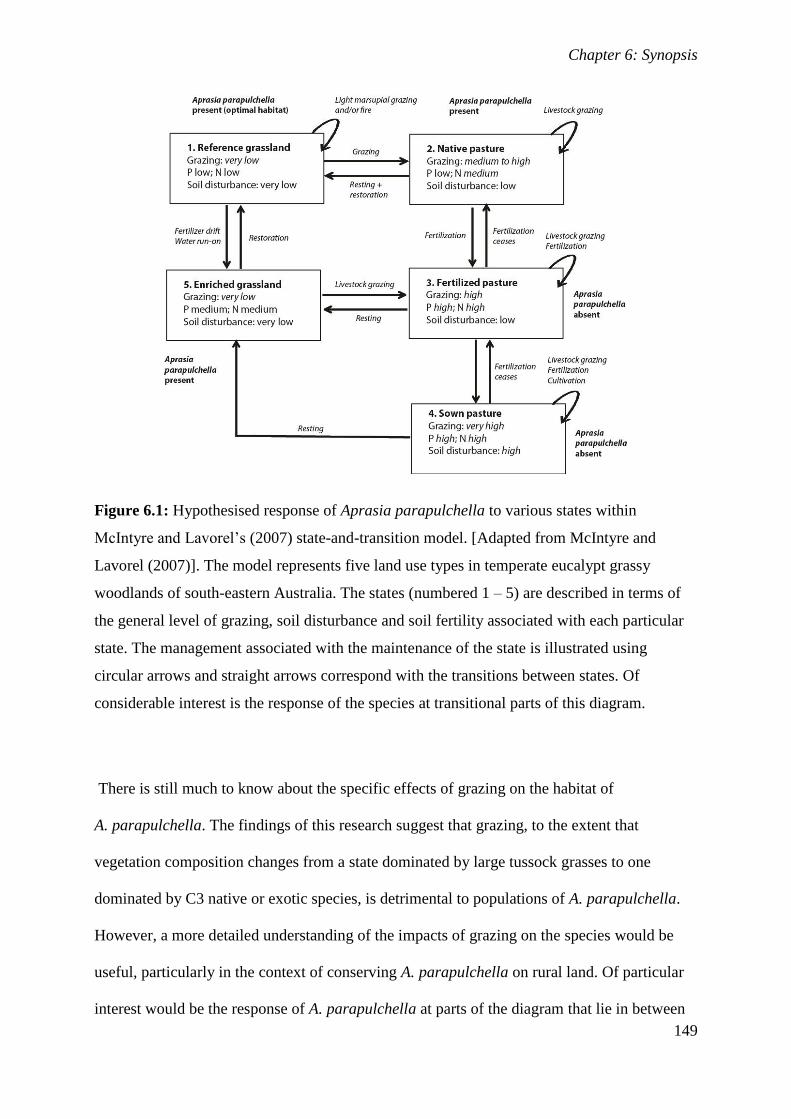
Chapter 6: Synopsis
149
Figure 6.1: Hypothesised response of Aprasia parapulchella to various states within
McIntyre and Lavorel’s (2007) state-and-transition model. [Adapted from McIntyre and
Lavorel (2007)]. The model represents five land use types in temperate eucalypt grassy
woodlands of south-eastern Australia. The states (numbered 1 – 5) are described in terms of
the general level of grazing, soil disturbance and soil fertility associated with each particular
state. The management associated with the maintenance of the state is illustrated using
circular arrows and straight arrows correspond with the transitions between states. Of
considerable interest is the response of the species at transitional parts of this diagram.
There is still much to know about the specific effects of grazing on the habitat of
A. parapulchella. The findings of this research suggest that grazing, to the extent that
vegetation composition changes from a state dominated by large tussock grasses to one
dominated by C3 native or exotic species, is detrimental to populations of A. parapulchella.
However, a more detailed understanding of the impacts of grazing on the species would be
useful, particularly in the context of conserving A. parapulchella on rural land. Of particular
interest would be the response of A. parapulchella at parts of the diagram that lie in between
Chapter 6: Synopsis
150
the discrete states (in reality, these may constitute intermediate states between those identified
– e.g. Aristida ramosa dominated pasture as an intermediate state between Themeda triandra
grassland [state 1] and Austrostipa/Austrodanthonia dominated native pasture [state 2]).
Whilst research suggests that stock exclusion from rocky areas may be beneficial for
conserving reptile biodiversity (Michael et al. 2008), the effect of stock exclusion requires
further investigation. To this end, experiments which investigate the impacts of grazing and
stock exclusion on A. parapulchella and other reptiles, would help to inform conservation
efforts not only for A. parapulchella, but also a range of other flora and fauna associated with
rocky outcrops (Michael et al. 2008).
The results of the analysis of the factors affecting the abundance of A. parapulchella at
the patch scale suggested that there may be complex interactions taking place between the
resources upon which A. parapulchella depends (ants, rocks and native grasses) and other
resources such as soil minerals and micro-organisms. Investigations that aimed to further
tease apart these relationships and the impact of agricultural practices could provide valuable
insights relating to, not only A. parapulchella, but also other plant, vertebrate and invertebrate
taxa.
The finding that specimens of A. parapulchella are significantly larger-bodied in
Victoria, compared with the ACT, also warrants further attention. Genetic analysis would be
the best method of addressing this (Wong et al. 2011). Population genetic studies of the
various populations of A. parapulchella in Victoria, NSW and ACT will also provide
invaluable information on the genetic distance between populations and the effect of barriers
to movement that could inform conservation management actions targeted at the species.
The movement, dispersal and activity patterns of A. parapulchella are other areas in
which there is little available information. Jones (1999) investigated activity to some extent in
the laboratory. Examining this in the field remains somewhat challenging due to the small
Chapter 6: Synopsis
151
size and cryptic nature of the species. There may be potential to set up ant colonies within
large “ant-farm” style enclosures and observe the interactions between A. parapulchella and
the colonies. Though this would be logistically challenging, such an experiment may yield
very interesting insights about the, hitherto unknown, fossorial habits of the lizards.
Conclusions
Taken together, the findings of my research suggest that agricultural modification has been a
major agent of decline for A. parapulchella across its range. Maintaining the existing
populations in the ACT will require avoiding further habitat loss and disturbance caused by
the direct and indirect effects of urbanisation, forestry and agricultural activities. On
agricultural lands, this will be best achieved by quarantining areas containing
A. parapulchella from nutrient addition and managing grazing appropriately, including
considering grazing exclusion, if appropriate. In addition, maintaining connectivity between
rocky outcrops of suitable native grass cover is likely to facilitate movement between habitat
patches. Therefore, effective conservation of A. parapulchella on private land will only be
able to be achieved by working effectively with farmers and land managers.

Chapter 6: Synopsis
152
References
153
References
Abell R., Brown C., Finlayson D., Lenz S., Mayer W., McCue K., McQueen K., Pillans B.,
Rickard M. & Strusz D. (2008) Geology of the Australian Capital Territory. 1:100 000 scale
map. Geological Society of Australia (ACT Division), Canberra.
Anderson R. P., Lew D. & Peterson A. T. (2003) Evaluating predictive models of species'
distributions: criteria for selecting optimal models. Ecological Modelling 162, 211-32.
Austin G. E., Thomas C. J., Houston D. C. & Thompson D. B. A. (1996) Predicting the
Spatial Distribution of Buzzard Buteo buteo Nesting Areas Using a Geographical Information
System and Remote Sensing. Journal of Applied Ecology 33, 1541-50.
Austin M. (2007) Species distribution models and ecological theory: A critical assessment
and some possible new approaches. Ecological Modelling 200, 1-19.
Austin M. P. (2002) Spatial prediction of species distribution: an interface between ecological
theory and statistical modelling. Ecological Modelling 157, 101-18.
Australian Government Bureau of Meteorology. (2010) Climate statistics for Australian
locations: ACT. Available at:
http://www.bom.gov.au/climate/averages/tables/cw_070282.shtml. Accessed 2nd September
2010.
Ballinger R. E. (1979) Intraspecific variation in demography and life history of the lizard,
Sceloporus jarrovi, Along an altitudinal gradient in southeastern Arizona. Ecology 60, 901-9.
Barnosky A. D., Matzke N., Tomiya S., Wogan G. O. U., Swartz B., Quental T. B., Marshall
C., McGuire J. L., Lindsey E. L., Maguire K. C., Mersey B. & Ferrer E. A. (2011) Has the
Earth's sixth mass extinction already arrived? Nature 471, 51-7.
References
154
Barrer P. (1992) A survey of Aprasia parapulchella along parts of the lower Molonglo River
corridor. A report to the ACT Heritage Unit and the ACT Parks and Conservation Service
Wildlife Research Unit. Canberra.
Belliure J. & Carrascal Luis M. (2002) Influence of heat transmission mode on heating rates
and on the selection of patches for heating in a Mediterranean lizard. Physiological and
Biochemical Zoology 75, 369-76.
Benton T. G., Vickery J. A. & Wilson J. D. (2003) Farmland biodiversity: is habitat
heterogeneity the key? Trends in Ecology & Evolution 18, 182-8.
Bourg N. A., McShea W. J. & Gill D. E. (2005) Putting a CART before the search: successful
habitat prediction for a rare forest herb. Ecology 86, 2793-804.
Breiman L. (2001) Statistical modeling: The two cultures (with comments and a rejoinder by
the author). Statistical Science 16, 199-231.
Bromham L., Cardillo M., Bennett A. F. & Elgar M. A. (1999) Effects of stock grazing on the
ground invertebrate fauna of woodland remnants. Australian Journal of Ecology 24, 199-207.
Brook B. W., Sodhi N. S. & Bradshaw C. J. A. (2008) Synergies among extinction drivers
under global change. Trends in Ecology & Evolution 23, 453-60.
Brown G. W. (2001) The influence of habitat disturbance on reptiles in a Box-Ironbark
eucalypt forest of south-eastern Australia. Biodiversity and Conservation 10, 161-76.
Brown G. W. (2009) Field surveys for the endangered Pink-tailed Worm Lizard Aprasia
parapulchella around Bendigo, north-central Victoria. A report to the Goulburn-Broken
Catchment Management Authority. Arthur Rylah Institute for Environmental Research,
Department of Sustainability and the Environment, Heidelberg, Victoria.
Brown G. W., Bennett A. F. & Potts J. M. (2008) Regional faunal decline - reptile occurrence
in fragmented rural landscapes of south-eastern Australia. Wildlife Research 35, 8-18.
References
155
Brown G. W., Dorrough J. W. & Ramsey D. S. L. (in press) Landscape and local influences
on patterns of reptile occurrence in grazed temperate woodlands of southern Australia.
Landsc. Urban Plan. 103, 277-88.
Bureau of Rural Sciences Australian Collaborative Land Use and Management Practice
[ACLUMP]. (2009) Land use summary: Australia (19 October 2009). Bureau of Rural
Sciences, Australian Government, Canberra, Australia.
http://adl.brs.gov.au/landuse/index.cfm?fa=main.reporting. Accessed 28 March 2013.
Bureau of Rural Sciences Australian Collaborative Land Use and Management Practice
[ACLUMP]. (2010) Land use summary: ACT NRM region - ACT (19 August 2010). Bureau
of Rural Sciences. Australian Government., Canberra, Australia.
http://adl.brs.gov.au/landuse/index.cfm?fa=main.reporting. Accessed 28 March 2013.
Castellano M. J. & Valone T. J. (2006) Effects of livestock removal and perennial grass
recovery on the lizards of a desertified arid grassland. Journal of Arid Environments 66, 87-
95.
Chase J. M. & Leibold M. A. (2003) Ecological Niches: Linking Classical and Contemporary
Approaches. University of Chicago Press. Chicago, IL, USA.
Clarke P. J. (2003) Composition of grazed and cleared temperate grassy woodlands in eastern
Australia: patterns in space and inferences in time. Journal of Vegetation Science 14, 5-14.
Cogger H. G. (1992) Reptiles and Amphibians of Australia, 5th Edition. Reed Books,
Chatswood, Australia.
Cogger H. G., Cameron E. E., Sadlier R. A. & Eggler P. (1993) The action plan for
Australian reptiles. Australian Nature Conservation Agency Canberra, Australia.
Croak B. M., Pike D. A., Webb J. K. & Shine R. (2008, in press) Using artificial rocks to
restore nonrenewable shelter sites in human-degraded systems: colonization by fauna.
Restoration Ecology.
Crutzen P. J. (2002) Geology of mankind. Nature 415, 23.
References
156
Davies K. F., Margules C. R. & Lawrence J. F. (2004) A synergistic effect puts rare,
specialized species at greater risk of extinction. Ecology 85, 265-71.
De Lisle H. F. (1996) The Natural History of Monitor Lizards. Krieger Publishing Company,
Florida.
Dormann C. F. (2007) Promising the future? Global change projections of species
distributions. Basic and Applied Ecology 8, 387-97.
Dorrough J., Ash J., Bruce S. & McIntyre S. (2007) From plant neighbourhood to landscape
scales: how grazing modifies native and exotic plant species richness in grassland. Plant
Ecology 191, 185-98.
Dorrough J., McIntyre S., Brown G., Stol J., Barrett G. & Brown A. (2012) Differential
responses of plants, reptiles and birds to grazing management, fertilizer and tree clearing.
Austral Ecology 37, 569-82.
Dorrough J., Moxham C., Turner V. & Sutter G. (2006) Soil phosphorus and tree cover
modify the effects of livestock grazing on plant species richness in Australian grassy
woodland. Biological Conservation 130, 394-405.
Dorrough J. & Scroggie M. P. (2008) Plant responses to agricultural intensification. Journal
of Applied Ecology 45, 1274-83.
Dunham A. E., Grant B. W. & Overall K. L. (1989) Interfaces between biophysical and
physiological ecology and the population ecology of terrestrial vertebrate ectotherms.
Physiological Zoology 62, 335-55.
Ecology Partners Pty Ltd. (2009) Hume highway duplication: threatened reptile monitoring
2007/08, New South Wales. Unpublished report for Roads and Traffic Authority. Ecology
Parners Pty Ltd, Brunswick, Victoria.
Elith J., Graham C. G., Anderson R. P., Dudík M., Ferrier S., Guisan A., Hijmans R. J.,
Huettmann F., Leathwick J. R., Lehmann A., Li J., Lohmann L. G., Loiselle B. A., Manion
G., Moritz C., Nakamura M., Nakazawa Y., Overton J., McC. M. , Peterson A. T., Phillips S.
References
157
J., Richardson K., Scachetti-Pereira R., Schapire R. E., Soberón J., Williams S., Wisz M. S. &
Zimmermann N. E. (2006) Novel methods improve prediction of species' distributions from
occurrence data. Ecography 29, 129-51.
Elith J., Leathwick J. & Hastie T. (2008) A working guide to boosted regression trees.
Journal of Animal Ecology 77, 802-13.
Elith J. & Leathwick J. R. (2009) Species Distribution Models: Ecological Explanation and
Prediction Across Space and Time. Annual Review of Ecology, Evolution, and Systematics 40,
677-97.
Elith J., Phillips S. J., Hastie T., Dudik M., Chee Y. E. & Yates C. J. (2011) A statistical
explanation of MaxEnt for ecologists. Diversity and Distributions 17, 43-57.
Elton C. (1927) Animal Ecology, London.
Engler R., Guisan A. & Rechsteiner L. (2004) An improved approach for predicting the
distribution of rare and endangered species from occurrence and pseudo-absence data.
Journal of Applied Ecology 41, 263-74.
Environmental Research and Information Consortium. (2001) Remote sensing detection of
native grasslands using multi-image spectral analysis - south eastern highlands of NSW.
Report prepared for New South Wales National Parks and Wildlife Service, Canberra,
Australian Captial Territory, Australia.
Ferrier S., Watson G., Pearce J. & Drielsma M. (2002) Extended statistical approaches to
modelling spatial pattern in biodiversity in northeast New South Wales. I. Species-level
modelling. Biodiversity and Conservation 11, 2275-307.
Fielding A. H. & Bell J. F. (2002) A review of methods for the assessment of prediction
errors in conservation presence/absence models. Environmental conservation 24, 38-49.
Finlayson D. M. (2008) A Geological Guide to Canberra Region and Namadgi National
Park. Geological Society of Australia, Australian Capital Territory, Australia.
References
158
Ford H. A., Barrett G. W., Saunders D. A. & Recher H. F. (2001) Why have birds in the
woodlands of Southern Australia declined? Biological Conservation 97, 71-88.
Foster D., Swanson F., Aber J., Burke I., Brokaw N., Tilman D. & Knapp A. (2003) The
importance of land-use legacies to ecology and conservation. BioScience 53, 77-88.
Foufopoulos J. & Ives A. R. (1999) Reptile extinctions on land-bridge islands: life-history
attributes and vulnerability to extinction. The American Naturalist 153, 1-25.
Franklin J. (2009) Mapping species distributions: spatial inference and prediction.
Cambridge University Press, Cambridge.
Gadsden H., Ballesteros-Barrera C., Hinojosa de la Garza O., Castañeda G., García-De la
Peña C. & Lemos-Espinal J. A. (2012) Effects of land-cover transformation and climate
change on the distribution of two endemic lizards, Crotaphytus antiquus and Sceloporus
cyanostictus, of northern Mexico. Journal of Arid Environments 83, 1-9.
Garden J. G., McAlpine C. A., Possingham H. P. & Jones D. N. (2007) Habitat structure is
more important than vegetation composition for local-level management of native terrestrial
reptile and small mammal species living in urban remnants: A case study from Brisbane,
Australia. Austral Ecology 32, 669-85.
Garrick D. (2008) Body surface temperature and length in relation to the thermal biology of
lizards. Bioscience Horizons 1, 136-42.
Ghiselin M. T. (1974) The Economy of Nature and the Evolution of Sex. University of
California Press, Berkeley.
Grinnell J. (1917) Field tests of theories concerning distributional control. The American
Naturalist 51, 115-28.
Groves R. H., Austin M. P. & Kaye P. E. (2003) Competition between Australian native and
introduced grasses along a nutrient gradient. Austral Ecology 28, 491-8.
References
159
Guisan A., Bronnimann O., Engler R., Vust M., Yoccoz N. G., Lehmann A. & Zimmermann
N. E. (2006a) Using niche-based models to improve the sampling of rare species.
Conservation Biology 20, 501-11.
Guisan A., Lehmann A., Ferrier S., Austin M. P., Overton J., Aspinall R. & Hastie T. (2006b)
Making better biogeographical predictions of species' distributions. Journal of Applied
Ecology 43, 386-92.
Guisan A. & Thuiller W. (2005) Predicting species distribution: offering more than simple
habitat models. Ecology Letters 8, 993-1009.
Guisan A. & Zimmermann N. E. (2000) Predictive habitat distribution models in ecology.
Ecological Modelling 135, 147-86.
Hampe A. (2004) Bioclimate envelope models: what they detect and what they hide. Global
Ecology and Biogeography 13, 469-71.
Hanley J. A. & NcNeil B. S. (1982) The meaning and use of the area under a receiver
operating characteristic
(ROC) curve. Radiology 143, 29-36.
Hastie T. & Tibshirani R. (1986) Generalized additive models. Statistical Science 1, 297-318.
Hastie T., Tibshirani R. & Friedman J. (2009) The Elements of Statistical Learning. New
York: Springer.
Heatwole H. F. & Taylor J. (1987) Ecology of Reptiles. Surrey Beatty and Sons, Chipping
Norton, NSW.
Heikkinen R. K., Luoto M., Virkkala R., Pearson R. G. & Körber J.-H. (2007) Biotic
interactions improve prediction of boreal bird distributions at macro-scales. Global Ecology
and Biogeography 16, 754-63.
References
160
Henle K. (1989) Ecological segregation in an assemblage of diurnal lizards in arid Australia.
Australian National University, Canberra.
Hernandez P. A., Graham C. H., Master L. L. & Albert D. L. (2006) The effect of sample size
and species characteristics on performance of different species distribution modeling methods.
Ecography 29, 773-85.
Hero J. M. & Morrison C. (2002) Frog declines in Australia: Global implications. In:
Symposium of the Society for Conservation Biology pp. 175-86. British Herpetol Soc,
Canterbury, England.
Hirzel A. H. & Le Lay G. (2008) Habitat suitability modelling and niche theory. Journal of
Applied Ecology 45, 1372-81.
Hobbs R. J. (2001) Synergisms among habitat fragmentation, livestock grazing, and biotic
invasions in southwestern Australia. Conservation Biology 15, 1522-8.
Hoffmann M., Hilton-Taylor C., Angulo A., Böhm M., Brooks T. M., Butchart S. H. M.,
Carpenter K. E., Chanson J., Collen B., Cox N. A., Darwall W. R. T., Dulvy N. K., Harrison
L. R., Katariya V., Pollock C. M., Quader S., Richman N. I., Rodrigues A. S. L., Tognelli M.
F., Vié J.-C., Aguiar J. M., Allen D. J., Allen G. R., Amori G., Ananjeva N. B., Andreone F.,
Andrew P., Ortiz A. L. A., Baillie J. E. M., Baldi R., Bell B. D., Biju S. D., Bird J. P., Black-
Decima P., Blanc J. J., Bolaños F., Bolivar-G W., Burfield I. J., Burton J. A., Capper D. R.,
Castro F., Catullo G., Cavanagh R. D., Channing A., Chao N. L., Chenery A. M., Chiozza F.,
Clausnitzer V., Collar N. J., Collett L. C., Collette B. B., Fernandez C. F. C., Craig M. T.,
Crosby M. J., Cumberlidge N., Cuttelod A., Derocher A. E., Diesmos A. C., Donaldson J. S.,
Duckworth J. W., Dutson G., Dutta S. K., Emslie R. H., Farjon A., Fowler S., Freyhof J.,
Garshelis D. L., Gerlach J., Gower D. J., Grant T. D., Hammerson G. A., Harris R. B.,
Heaney L. R., Hedges S. B., Hero J.-M., Hughes B., Hussain S. A., M J. I., Inger R. F., Ishii
N., Iskandar D. T., Jenkins R. K. B., Kaneko Y., Kottelat M., Kovacs K. M., Kuzmin S. L.,
Marca E. L., Lamoreux J. F., Lau M. W. N., Lavilla E. O., Leus K., Lewison R. L.,
Lichtenstein G., Livingstone S. R., Lukoschek V., Mallon D. P., McGowan P. J. K., McIvor
A., Moehlman P. D., Molur S., Alonso A. M., Musick J. A., Nowell K., Nussbaum R. A.,
Olech W., Orlov N. L., Papenfuss T. J., Parra-Olea G., Perrin W. F., Polidoro B. A.,
References
161
Pourkazemi M., Racey P. A., Ragle J. S., Ram M., Rathbun G., Reynolds R. P., Rhodin A. G.
J., Richards S. J., Rodríguez L. O., Ron S. R., Rondinini C., Rylands A. B., Mitcheson Y. S.
d., Sanciangco J. C., Sanders K. L., Santos-Barrera G., Schipper J., Self-Sullivan C., Shi Y.,
Shoemaker A., Short F. T., Sillero-Zubiri C., Silvano D. L., Smith K. G., Smith A. T., Snoeks
J., Stattersfield A. J., Symes A. J., Taber A. B., Talukdar B. K., Temple H. J., Timmins R.,
Tobias J. A., Tsytsulina K., Tweddle D., Ubeda C., Valenti S. V., Dijk P. P. v., Veiga L. M.,
Veloso A., Wege D. C., Wilkinson M., Williamson E. A., Xie F., Young B. E., Akçakaya H.
R., Bennun L., Blackburn T. M., Boitani L., Dublin H. T., Fonseca G. A. B. d., Gascon C.,
Lacher T. E., Mace G. M., Mainka S. A., McNeely J. A., Mittermeier R. A., Reid G. M.,
Rodriguez J. P., Rosenberg A. A., Samways M. J., Smart J., Stein B. A. & Stuart S. N. (2010)
The impact of conservation on the status of the world’s vertebrates. Science 330, 1503-9.
Houlder D., Hutchinson M. F., Nix H. A. & McMahon J. P. (2000) ANUCLIM User's Guide.
Centre for Resource and Environmental Studies, Australian National University, Canberra,
Australia.
Houniet D. T., Thuiller W. & Tolley K. A. (2009) Potential effects of predicted climate
change on the endemic South African Dwarf Chameleons, Bradypodion. African Journal of
Herpetology 58, 28-35.
Hutchinson G. E. (1957) Concluding remarks. Cold Spring Harbor Symposium on
Quantitative Biology 22, 415-27.
Ivlev V. S. (1961) Experimental Ecology of the Feeding of Fishes. Yale University Press,
Connecticut.
Jaksic F. M. & Greene H. W. (1984) Empirical evidence of non-correlation between tail loss
frequency and predation intensity on lizards. Oikos 42, 407-11.
James C. D. (2003) Response of vertebrates to fenceline contrasts in grazing intensity in semi-
arid woodlands of eastern Australia. Austral Ecology 28, 137-51.
Jenkins R. W. G. & Bartell R. J. (1980) A Field Guide to Reptiles of the Australian High
Country. Inkata Press, Melbourne.
References
162
Jennings W. B., Pianka E. R. & Donnellan S. (2003) Systematics of the lizard family
Pygopodidae with implications for the diversification of Australian temperate biotas.
Systematic Biology 52, 757 - 80.
Jones S. R. (1992) Habitat relationships, diet and abundance of the endangered Pygopodid,
Aprasia parapulchella in the Australian Capital Territory and surrounding New South Wales.
Bachelor of Applied Science (Honours) Thesis. Applied Ecology Research Group, University
of Canberra, Canberra.
Jones S. R. (1999) Conservation biology of the Pink-tailed Legless Lizard Aprasia
parapulchella. PhD thesis. Applied Ecology Research Group. University of Canberra,
Canberra, Australia.
Klimek S., Richter gen. Kemmermann A., Hofmann M. & Isselstein J. (2007) Plant species
richness and composition in managed grasslands: The relative importance of field
management and environmental factors. Biological Conservation 134, 559-70.
Kluge A. (1974) A taxonomic revision of the lizard family Pygopodidae. Miscelaneous
Publications, Museum of Zoology, University of Mischigan 147, 1-221.
Kotsonis A. & Joyce B. (2003) Regolith mapping at Bendigo, and its relationship to gold in
Central Victoria, Australia. In: Advances in Regolith (ed I. C. Roach) pp. 239-43. CRC
LEME.
Koy K. (2009) Using the ArcMap model builder to clip, and export to multiple ascii raster
files. Geospatial Innovation Facility. http://creativecommons.org/licenses/by-sa/3.0/us/.
Accessed 2nd September 2010.
Kutt A. S. & Woinarski J. C. Z. (2007) The effects of grazing and fire on vegetation and the
vertebrate assemblage in a tropical savanna woodland in north-eastern Australia. Journal of
Tropical Ecology 23, 95-106.
Langston A. C. (1996) The ecology and distribution of Tympanocryptis lineata pinguicolla
(Southern Lined Earless Dragon) in the Australian Capitatl Territory and adjacent sub-region.
References
163
Bachelor of Applied Science (Honours) thesis. Applied Ecology Research Group, University
of Canberra, Canberra.
Lehmann A., Overton J. M. & Leathwick J. R. (2002) GRASP: generalized regression
analysis and spatial prediction. Ecological Modelling 157, 189-207.
Lippitt C. D., Rogan J., Toledano J., Sangermano F., Eastman J. R., Mastro V. & Sawyer A.
(2008) Incorporating anthropogenic variables into a species distribution model to map gypsy
moth risk. Ecological Modelling 210, 339-50.
Loiselle B. A., Howell C. A., Graham C. H., Goerk J. M., Brooks T., Smith K. G. & Williams
P. H. (2003) Avoiding pitfalls of using species distribution models in conservation planning.
Conservation Biology 17, 1591-600.
Luoto M., Heikkinen R. K., Pöyry J. & Saarinen K. (2006) Determinants of the
biogeographical distribution of butterflies in boreal regions. Journal of Biogeography 33,
1764-78.
Mackey B. G. & Lindenmayer D. B. (2001) Towards a hierarchical framework for modelling
the spatial distribution of animals. Journal of Biogeography 28, 1147-66.
Manel S., Williams H. C. & Ormerod S. J. (2001) Evaluating presence-absence models in
ecology: the need to account for prevalence. Journal of Applied Ecology 38, 921-31.
Mangel M., Talbot L. M., Meffe G. K., Agardy M. T., Alverson D. L., Barlow J., Botkin D.
B., budowski G., Clark T., Cooke J., Crozier R. H., Dayton P. K., Elder D. L., Fowler C. W.,
Funtowicz S., Giske J., Hofman R. J., Holt S. J., Kellert S. R., Kimball L. A., Ludgwig D.,
Magnusson K., Malayang B. S. I., Mann C., Norse E. A., Northridge S. P., Perrin W. F.,
Perrings C., Peterman R. M., Rabb G. B., Regier H. A., Reynolds J. E., Sherman K.,
Sissenwine M. P., Smith T. D., Starfield A., Taylor R. J., Tillman M. F., Toft C., Twiss J. R.
J., Wilen J. & Young T. P. (1996) Principles for the conservation of wild living resources.
Ecological Applications 6, 338-62.
References
164
Maron M. & Lill A. (2005) The influence of livestock grazing and weed invasion on habitat
use by birds in grassy woodland remnants. Biological Conservation 124, 439-50.
Martínez-Freiría F., Sillero N., Lizana M. & Brito J. C. (2008) GIS-based niche models
identify environmental correlates sustaining a contact zone between three species of European
vipers. Diversity and Distributions 14, 452-61.
McIntyre S. (2005) Biodiversity attributes of different sward structures in grazed grassland.
Ecological Management & Restoration 6, 71-3.
McIntyre S. (2008) The role of plant leaf attributes in linking land use to ecosystem function
in temperate grassy vegetation. Agriculture, Ecosystems & Environment 128, 251-8.
McIntyre S. & Lavorel S. (2007) A conceptual model of land use effects on the structure and
function of herbaceous vegetation. Agriculture, Ecosystems & Environment 119, 11-21.
McIntyre S. & Tongway D. (2005) Grassland structure in native pastures: links to soil surface
condition. Ecological Management & Restoration 6, 43-50.
McKinney M. L. & Lockwood J. L. (1999) Biotic homogenization: a few winners replacing
many losers in the next mass extinction. Trends in Ecology & Evolution 14, 450-3.
McLaughlin A. & Mineau P. (1995) The impact of agricultural practices on biodiversity.
Agriculture, Ecosystems & Environment 55, 201-12.
Medel R. G., Jimenez J. E., Fox S. F. & Jaksic F. M. (1988) Experimental evidence that high
population frequencies of lizard tail autotomy indicate inefficient predation. Oikos 53, 321-4.
Michael D. R. (2004) Distribution, habitat preferences and conservation status of reptiles in
the Albury-Wodonga region. The Victorian Naturalist 121, 180-93.
Michael D. R. (2007) A reptile survey on Nail Can Hill Flora and Fauna Reserve: summary of
results. Unpublished report to GHD, Wodonga, Victoria.
References
165
Michael D. R., Cunningham R. B. & Lindenmayer D. B. (2008) A forgotten habitat? Granite
inselbergs conserve reptile diversity in fragmented agricultural landscapes. Journal of Applied
Ecology 45, 1742-52.
Michael D. R. & Herring M. W. (2005) Habitat of the pink-tailed worm lizard Aprasia
parapulchella in Albury, NSW. Herpetofauna 35, 103 - 11.
Mikhail E. H. (1976) Soils of the Bendigo District. Soil survey report No. 56. Department of
Agriculture, Victoria.
Miller J. (2010) Species distribution modeling. Geography Compass 4, 490-509.
Monterroso P., Brito J. C., Ferreras P. & Alves P. C. (2009) Spatial ecology of the European
wildcat in a Mediterranean ecosystem: dealing with small radio-tracking datasets in species
conservation. Journal of Zoology 279, 27-35.
New T. R. (2000) How useful are ant assemblages for monitoring habitat disturbance on
grasslands in south eastern Australia? Journal of Insect Conservation 4, 153-9.
NSW National Parks and Wildlife Service. (1999) Recovery Plan for the Pink-tailed Worm
Lizard. Draft for public comment. NSW National Parks and Wildlife Service, Hurstville,
NSW.
Olds A. D., Pitt K. A., Maxwell P. S. & Connolly R. M. (2012) Synergistic effects of reserves
and connectivity on ecological resilience. Journal of Applied Ecology 49, 1195-203.
Osborne W. & Wong D. (2010) Extent of potential Pink-tailed worm-lizard (Aprasia
parapulchella) habitat in the Stage 2 investigation area - East Molonglo. Report
commissioned by ACT Planning and Land Authority. Institute for Applied Ecology,
University of Canberra, Canberra.
Osborne W. S. & Coghlan R. (2004) Distribution of the Pink-tailed Worm Lizard in the
Lower Molonglo Valley, ACT, with respect to strategic land planning.
References
166
Osborne W. S., Lintermans M. & Williams K. D. (1991) Distribution and conservation status
of the endangered Pink-tailed Legless Lizard (Aprasia parapulchella) (Kluge). Research
Report 5. ACT Parks and Conservation Service, Canberra.
Osborne W. S. & McKergow F. V. C. (1993) Distribution, population density and habitat of
the Pink-tailed Legless Lizard (Aprasia parapulchella) in Canberra Nature Park. Technical
Report No. 3. ACT Parks and Conservation Service, Canberra.
Patchell F. C. & Shine R. (1986) Food habits and reproductive biology of the Australian
legless lizards (Pygopodidae). Copeia 1986, 30-9.
Pawar S., Koo M. S., Kelley C., Ahmed M. F., Chaudhuri S. & Sarkar S. (2007) Conservation
assessment and prioritization of areas in Northeast India: Priorities for amphibians and
reptiles. Biological Conservation 136, 346-61.
Pearce J. & Ferrier S. (2000) Evaluating the predictive performance of habitat models
developed using logistic regression. Ecological Modelling 133, 225-45.
Pearce J. & Lindenmayer D. (1998) Bioclimatic analysis to enhance reintroduction biology of
the endangered helmeted honeyeater (Lichenostomus melanops cassidix) in southeastern
Australia. Restoration Ecology 6, 238-43.
Pearson R. G. (2007) Species' distribution modelling for conservation educators and
practitioners. Synthesis. American Museum of Natural History. Available at:
http:\\ncep.amnh.org. Accessed on 10th August 2010.
Pearson R. G. & Dawson T. P. (2004) Bioclimate envelope models: what they detect and
what they hide — response to Hampe (2004). Global Ecology and Biogeography 13, 471-3.
Pearson R. G., Dawson T. P. & Liu C. (2004) Modelling species distributions in Britain: a
hierarchical integration of climate and land-cover data. Ecography 27, 285-98.
Pearson R. G., Raxworthy C. J., Nakamura M. & Townsend Peterson A. (2007) Predicting
species distributions from small numbers of occurrence records: a test case using cryptic
geckos in Madagascar. Journal of Biogeography 34, 102-17.
References
167
Pereira H. M., Leadley P. W., Proença V., Alkemade R., Scharlemann J. P. W., Fernandez-
Manjarrés J. F., Araújo M. B., Balvanera P., Biggs R., Cheung W. W. L., Chini L., Cooper H.
D., Gilman E. L., Guénette S., Hurtt G. C., Huntington H. P., Mace G. M., Oberdorff T.,
Revenga C., Rodrigues P., Scholes R. J., Sumaila U. R. & Walpole M. (2010) Scenarios for
Global Biodiversity in the 21st Century. Science 330, 1496-501.
Perrings C., Jackson L., Bawa K., Brussaard L., Brush S., Gavin T., Papa R., Pascual U. & De
Ruiter P. (2006) Biodiversity in Agricultural Landscapes: Saving Natural Capital without
Losing Interest. Conservation Biology 20, 263-4.
Pettit N. E., Froend R. H. & Ladd P. G. (1995) Grazing in remnant woodland vegetation:
changes in species composition and life form groups. Journal of Vegetation Science 6, 121-
30.
Phillips S. J. (2006) A brief tutorial on Maxent. AT & T Research. Available at:
http://www.cs.princeton.edu/~schapire/maxent/tutorial/tutorial.doc. Accessed 25th September
2011.
Phillips S. J., Anderson R. P. & Schapire R. E. (2006) Maximum entropy modeling of species
geographic distributions. Ecological Modelling 190, 231-59.
Phillips S. J. & Dudík M. (2008) Modeling of species distributions with Maxent: new
extensions and a comprehensive evaluation. Ecography 31, 161-75.
Phillips S. J., Dudík M. & Schapire R. E. (2004) A maximum entropy approach to species
distribution modeling. In: Proceedings of the twenty-first international conference on
Machine learning pp. 83-. ACM, Banff, Alberta, Canada.
Pike D. A., Croak B. M., Webb J. K. & Shine R. (2010) Subtle – but easily reversible –
anthropogenic disturbance seriously degrades habitat quality for rock-dwelling reptiles.
Animal Conservation 13, 411-8.
Pimm S., Russell G., Gittleman J. & Brooks T. (1995) The future of biodiversity. Science
269, 347-50.
References
168
Pimm S. L. (2008) Biodiversity: Climate Change or Habitat Loss - Which Will Kill More
Species. Current Biology 18, R117-R9.
Porembski S. & Barthlott W. (2000) Granitic and gneissic outcrops (inselbergs) as centers of
diversity for desiccation-tolerant vascular plants. Plant Ecology 151, 19-28.
Pough F. H. & Gans C. (1982) The Vocabulary of Reptilian Thermoregulation. In: Biology of
the Reptilia (ed C. Gans) pp. 17-23. New York: Academic Press.
Pringle R. M., Webb J. K. & Shine R. (2003) Canopy structure, microclimate, and habitat
selection by a nocturnal snake, Hoplocephalus bungaroides. Ecology 84, 2668-79.
Pulliam H. R. (2000) On the relationship between niche and distribution. Ecology Letters 3,
349-61.
Purvis A., Gittleman J. L., Cowlishaw G. & Mace G. M. (2000) Predicting extinction risk in
declining species. Proceedings: Biological Sciences 267, 1947-52.
R Development Core Team. (2005) R: A Language and Environment. Vienna, Austria.
Rankin P. R. (1976) A note on the possible diversionary defence mechanism in the worm
lizard Aprasia parapulchella Kluge. Herpetofauna 8, 18-9.
Raxworthy C. J., Martinez-Meyer E., Horning N., Nussbaum R. A., Schneider G. E., Ortega-
Huerta M. A. & Townsend Peterson A. (2003) Predicting distributions of known and
unknown reptile species in Madagascar. Nature 426, 837-41.
Rehwinkel R. (2007) A method to assess grassy ecosystem sites: using floristic information to
assess a site's quality. NSW Department of Environment and Climate Change, Queanbeyan,
NSW, Australia.
Richter D. D., Markewitz D., Heine P. R., Jin V., Raikes J., Tian K. & Wells C. G. (2000)
Legacies of agriculture and forest regrowth in the nitrogen of old-field soils. Forest Ecology
and Management 138, 233-48.
References
169
Ridgeway G. (2006) Generalized boosted regression models. Documentation on the R
Package ‘gbm’, version 1.5 - 7.
http://phase.hpcc.jp/mirrors/stat/R/CRAN/doc/packages/gbm.pdf. Accessed 26 March 2013.
Riley J., Stimson A. F. & Winch J. M. (1985) A review of Squamata ovipositing in ant and
termite nests. Herpetological Review 16, 38-43.
Robertson P. & Heard G. W. (2008) Report on field surveys for the Pink-tailed Worm Lizard
(Aprasia parapulchella) in the Bendigo region, central Victoria: distributiion, habitat,
associations and population attributes. Report prepared for Department of Sustainability and
Environment. Wildife Profiles Pty Ltd, Heidelberg, Victoria.
Robinson W. A. (1996) Ant communities in the grasslands of the Australian Capital Territory
and the role of ants in the ecology of the pink-tailed legless lizard, Aprasia parapulchella.
MSc thesis. University of Canberra, Canberra.
Royle J. A., Chandler R. B., Yackulic C. & Nichols J. D. (2012) Likelihood analysis of
species occurrence probability from presence-only data for modelling species distributions.
Methods in Ecology and Evolution 3, 545-54.
Rummery C., Shine R., Houston D. L. & Thompson M. B. (1995) Thermal biology of the
Australian forest dragon, Hypsilurus spinipes (Agamidae). Copeia 1994, 818-27.
Sass S., Watson D. & Wilson A. (2008) The reptile fauna of the upper Billabong Creek
catchment area, southern New South Wales. Herpetofauna 38, 41-50.
Schoener T. W. (1979) Inferring the properties of predation and other injury-producing agents
from injury frequency. Ecology 60, 1110-5.
Seoane J., Bustamante J. & Dıaz-Delgado R. (2004) Competing roles for landscape,
vegetation, topography and climate in predictive models of bird distribution. Ecological
Modelling 171, 209-22.
Sharp S. (2006) Assessment of vegetation condition of grassy ecosystems in the Australian
Capital Territory. Ecological Management & Restoration 7, S63-S5.
References
170
Sillero N. (2011) What does ecological modelling model? A proposed classification of
ecological niche models based on their underlying methods. Ecological Modelling 222, 1343-
6.
Stockwell D. & Peters D. (1999) The GARP - modelling system: problems and solutions to
automated spatial prediction. International Journal of Geographical Information Science 13,
143-.
Stuwe J. & Parsons R. F. (1977) Themeda australis grasslands on the Basalt Plains, Victoria:
floristics and management effects. Austral Ecology 2, 467-76.
Swenson N. G. (2008) The past and future influence of geographic information systems on
hybrid zone, phylogeographic and speciation research. Journal of Evolutionary Biology 21,
421-34.
Swets J. A. (1988) Measuring the accuracy of diagnostic systems. Science 240, 1285-93.
Thuiller W. (2003) BIOMOD - optimizing predictions of species distributions and projecting
potential future shifts under global change. Global Change Biology 9, 1353-62.
Thuiller W., Albert C., Araújo M. B., Berry P. M., Cabeza M., Guisan A., Hickler T.,
Midgley G. F., Paterson J., Schurr F. M., Sykes M. T. & Zimmermann N. E. (2008)
Predicting global change impacts on plant species' distributions: Future challenges.
Perspectives in Plant Ecology, Evolution and Systematics 9, 137-52.
Tingley R. & Herman T. B. (2009) Land-cover data improve bioclimatic models for anurans
and turtles at a regional scale. Journal of Biogeography 36, 1656-72.
Tinkle D. W. & Ballinger R. E. (1972) Sceloporus undulatus: a study of the intraspecific
comparative demography of a lizard. Ecology 53, 570-84.
Urban D. L., O'Neill R. V. & Shugart H. H. (1987) Landscape Ecology: a hierarchical
perspective can help scientists understand spatial patterns. BioScience 37, 119-27.
References
171
Van Niel K. P., Laffan S. W. & Lees B. G. (2004) Effect of error in the DEM on
environmental variables for predictive vegetation modelling. Journal of Vegetation Science
15, 747-56.
Vandermeer J. H. (1972) Niche Theory. Annual Review of Ecology and Systematics 3, 107-
32.
Velásquez-Múnera E., Ortiz-Reyes A., Páez V. & Guzmán-Restrepo G. E. (2008) Oviposition
of Stenorrhina degenhardti (Serpentes: Colubridae) in a nest of Acromyrmex octospinosus
(Hymenoptera: Formicidae). Revista Actualidades Biológicas 30, 193-.
Venier L. A., Pearce J., McKee J. E., McKenney D. W. & Niemi G. J. (2004) Climate and
satellite-derived land cover for predicting breeding bird distribution in the Great Lakes Basin.
Journal of Biogeography 31, 315-31.
Virkkala R., Luoto M., Heikkinen R. K. & Leikola N. (2005) Distribution patterns of boreal
marshland birds: modelling the relationships to land cover and climate. Journal of
Biogeography 32, 1957-70.
Wainer J., Robertson P. & Yen A. (in prep.) Diet of the threatened Mallee Worm-Lizard
(Aprasia aurita) and the Pink-nosed Worm-Lizard (Aprasia inaurita) in north-western
Victoria.
Westoby M., Walker B. & Noy-Meir I. (1989) Opportunistic Management for Rangelands
Not at Equilibrium. Journal of Range Management 42, 266-74.
Wilson S. & Swan G. (2008) A Complete Guide to Reptiles of Australia. 2nd Edition. New
Holland Publishers (Australia), Sydney.
Woinarski J. C. Z. & Ash A. J. (2002) Responses of vertebrates to pastoralism, military land
use and landscape position in an Australian tropical savanna. Austral Ecology 27, 311-23.
Wong D. & Osborne W. (2010) Confirmatory surveys for Pink-tailed Worm Lizards (Aprasia
parapulchella) and additional mapping of habitat along the Molonglo River corridor between
References
172
Coppins Crossing and Tuggeranong Parkway, ACT. Report to commissioned by ACT
Planning and Land Authority. Institute for Applied Ecology, Canberra.
Wong D. T. Y., Jones S. R., Osborne W. S., Brown G. W., Robertson P., Michael D. R. &
Kay G. M. (2011) The life history and ecology of the Pink-tailed Worm-lizard Aprasia
parapulchella Kluge - a review. The Australian Zoologist 35, 927-40.
Zuur A. F., Ieno E. N., Walker N. J., Saveliev A. A. & Smith G. M. (2009) Mixed effects
models and extensions in ecology with R. Springer, New York.
173
Appendices
Appendix 1:
Wong D. T. Y., Jones S. R., Osborne W. S., Brown G. W., Robertson P., Michael D. R. &
Kay G. M. (2011) The life history and ecology of the Pink-tailed Worm-lizard Aprasia
parapulchella Kluge - a review. The Australian Zoologist 35, 927-40.
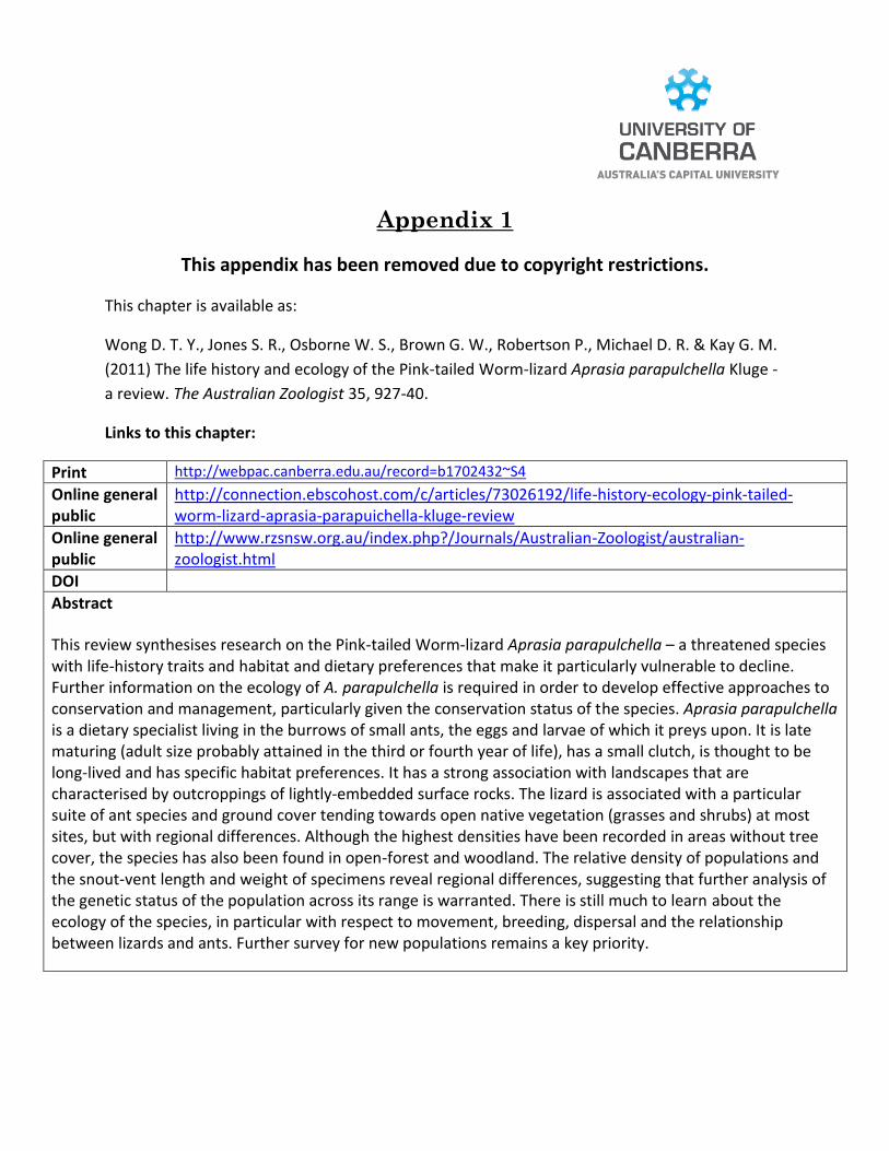
Appendix 1
This appendix has been removed due to copyright restrictions.
This chapter is available as:
Wong D. T. Y., Jones S. R., Osborne W. S., Brown G. W., Robertson P., Michael D. R. & Kay G. M.
(2011) The life history and ecology of the Pink-tailed Worm-lizard Aprasia parapulchella Kluge -
a review. The Australian Zoologist 35, 927-40.
Links to this chapter:
Print http://webpac.canberra.edu.au/record=b1702432~S4
Online general public
http://connection.ebscohost.com/c/articles/73026192/life-history-ecology-pink-tailed-worm-lizard-aprasia-parapuichella-kluge-review
Online general public
http://www.rzsnsw.org.au/index.php?/Journals/Australian-Zoologist/australian-zoologist.html
DOI
Abstract
This review synthesises research on the Pink-tailed Worm-lizard Aprasia parapulchella – a threatened species with life-history traits and habitat and dietary preferences that make it particularly vulnerable to decline. Further information on the ecology of A. parapulchella is required in order to develop effective approaches to conservation and management, particularly given the conservation status of the species. Aprasia parapulchella is a dietary specialist living in the burrows of small ants, the eggs and larvae of which it preys upon. It is late maturing (adult size probably attained in the third or fourth year of life), has a small clutch, is thought to be long-lived and has specific habitat preferences. It has a strong association with landscapes that are characterised by outcroppings of lightly-embedded surface rocks. The lizard is associated with a particular suite of ant species and ground cover tending towards open native vegetation (grasses and shrubs) at most sites, but with regional differences. Although the highest densities have been recorded in areas without tree cover, the species has also been found in open-forest and woodland. The relative density of populations and the snout-vent length and weight of specimens reveal regional differences, suggesting that further analysis of the genetic status of the population across its range is warranted. There is still much to learn about the ecology of the species, in particular with respect to movement, breeding, dispersal and the relationship between lizards and ants. Further survey for new populations remains a key priority.
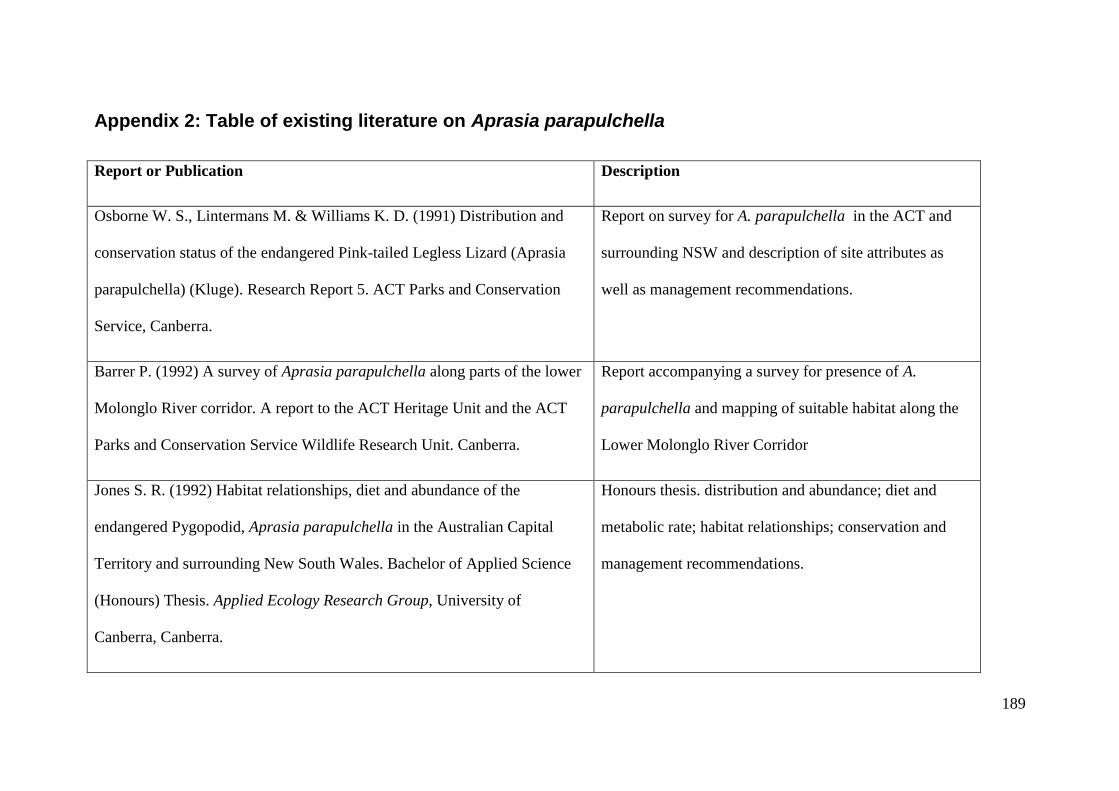
189
Appendix 2: Table of existing literature on Aprasia parapulchella
Report or Publication Description
Osborne W. S., Lintermans M. & Williams K. D. (1991) Distribution and
conservation status of the endangered Pink-tailed Legless Lizard (Aprasia
parapulchella) (Kluge). Research Report 5. ACT Parks and Conservation
Service, Canberra.
Report on survey for A. parapulchella in the ACT and
surrounding NSW and description of site attributes as
well as management recommendations.
Barrer P. (1992) A survey of Aprasia parapulchella along parts of the lower
Molonglo River corridor. A report to the ACT Heritage Unit and the ACT
Parks and Conservation Service Wildlife Research Unit. Canberra.
Report accompanying a survey for presence of A.
parapulchella and mapping of suitable habitat along the
Lower Molonglo River Corridor
Jones S. R. (1992) Habitat relationships, diet and abundance of the
endangered Pygopodid, Aprasia parapulchella in the Australian Capital
Territory and surrounding New South Wales. Bachelor of Applied Science
(Honours) Thesis. Applied Ecology Research Group, University of
Canberra, Canberra.
Honours thesis. distribution and abundance; diet and
metabolic rate; habitat relationships; conservation and
management recommendations.
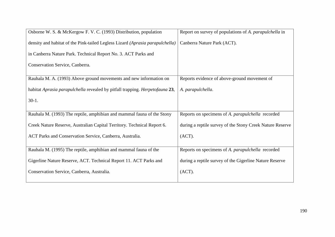
190
Osborne W. S. & McKergow F. V. C. (1993) Distribution, population
density and habitat of the Pink-tailed Legless Lizard (Aprasia parapulchella)
in Canberra Nature Park. Technical Report No. 3. ACT Parks and
Conservation Service, Canberra.
Report on survey of populations of A. parapulchella in
Canberra Nature Park (ACT).
Rauhala M. A. (1993) Above ground movements and new information on
habitat Aprasia parapulchella revealed by pitfall trapping. Herpetofauna 23,
30-1.
Reports evidence of above-ground movement of
A. parapulchella.
Rauhala M. (1993) The reptile, amphibian and mammal fauna of the Stony
Creek Nature Reserve, Australian Capital Territory. Technical Report 6.
ACT Parks and Conservation Service, Canberra, Australia.
Reports on specimens of A. parapulchella recorded
during a reptile survey of the Stony Creek Nature Reserve
(ACT).
Rauhala M. (1995) The reptile, amphibian and mammal fauna of the
Gigerline Nature Reserve, ACT. Technical Report 11. ACT Parks and
Conservation Service, Canberra, Australia.
Reports on specimens of A. parapulchella recorded
during a reptile survey of the Gigerline Nature Reserve
(ACT).
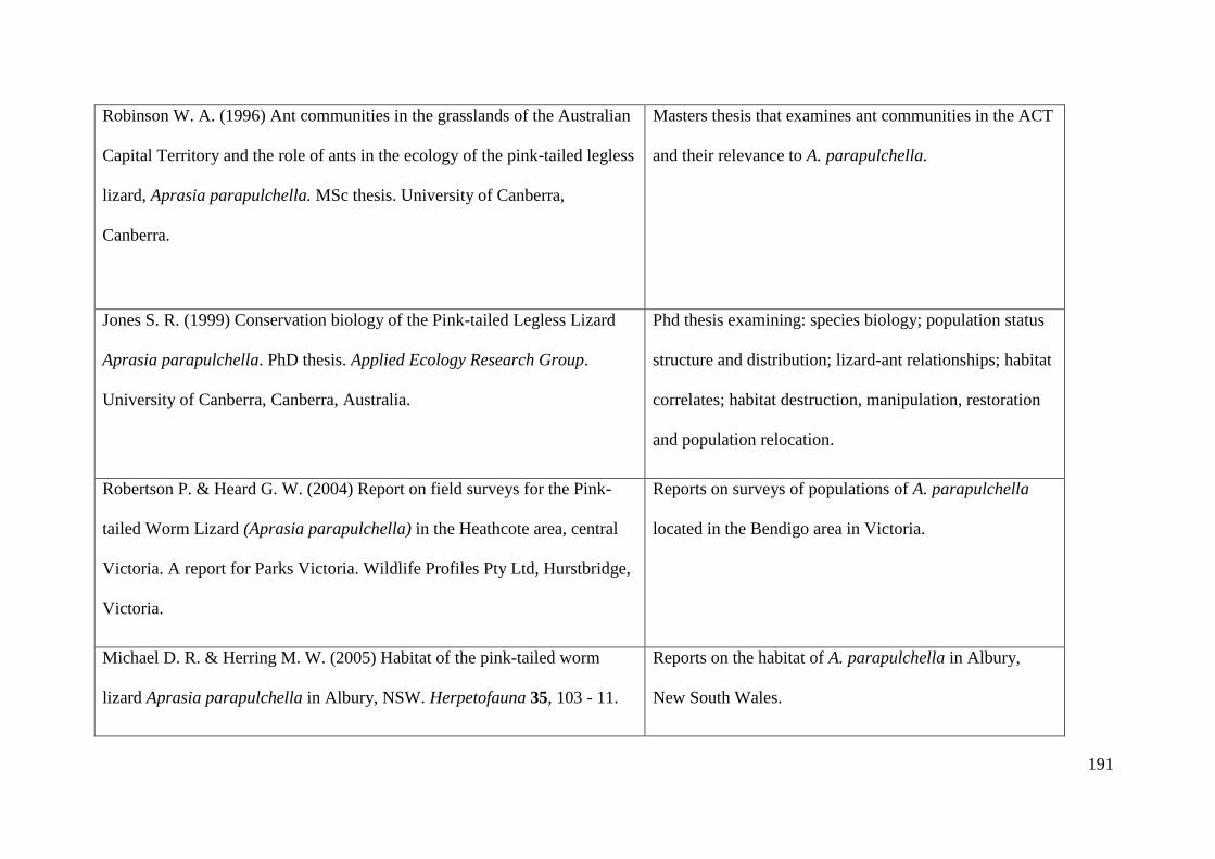
191
Robinson W. A. (1996) Ant communities in the grasslands of the Australian
Capital Territory and the role of ants in the ecology of the pink-tailed legless
lizard, Aprasia parapulchella. MSc thesis. University of Canberra,
Canberra.
Masters thesis that examines ant communities in the ACT
and their relevance to A. parapulchella.
Jones S. R. (1999) Conservation biology of the Pink-tailed Legless Lizard
Aprasia parapulchella. PhD thesis. Applied Ecology Research Group.
University of Canberra, Canberra, Australia.
Phd thesis examining: species biology; population status
structure and distribution; lizard-ant relationships; habitat
correlates; habitat destruction, manipulation, restoration
and population relocation.
Robertson P. & Heard G. W. (2004) Report on field surveys for the Pink-
tailed Worm Lizard (Aprasia parapulchella) in the Heathcote area, central
Victoria. A report for Parks Victoria. Wildlife Profiles Pty Ltd, Hurstbridge,
Victoria.
Reports on surveys of populations of A. parapulchella
located in the Bendigo area in Victoria.
Michael D. R. & Herring M. W. (2005) Habitat of the pink-tailed worm
lizard Aprasia parapulchella in Albury, NSW. Herpetofauna 35, 103 - 11.
Reports on the habitat of A. parapulchella in Albury,
New South Wales.
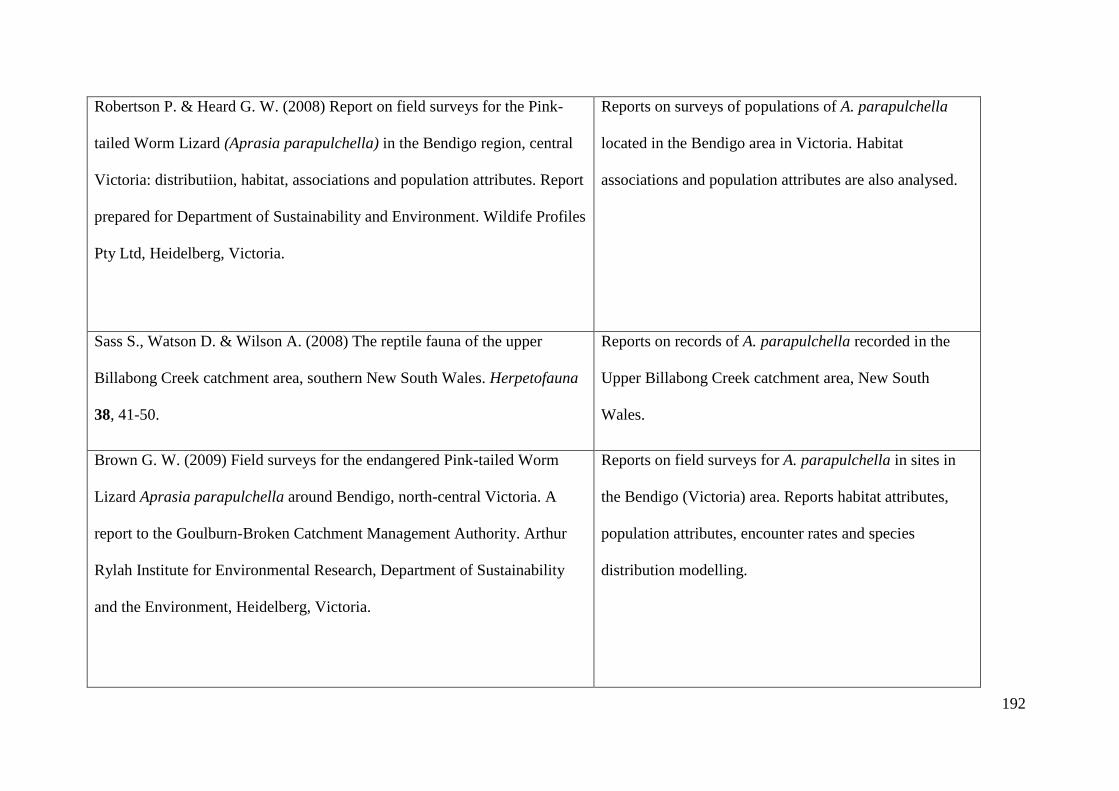
192
Robertson P. & Heard G. W. (2008) Report on field surveys for the Pink-
tailed Worm Lizard (Aprasia parapulchella) in the Bendigo region, central
Victoria: distributiion, habitat, associations and population attributes. Report
prepared for Department of Sustainability and Environment. Wildife Profiles
Pty Ltd, Heidelberg, Victoria.
Reports on surveys of populations of A. parapulchella
located in the Bendigo area in Victoria. Habitat
associations and population attributes are also analysed.
Sass S., Watson D. & Wilson A. (2008) The reptile fauna of the upper
Billabong Creek catchment area, southern New South Wales. Herpetofauna
38, 41-50.
Reports on records of A. parapulchella recorded in the
Upper Billabong Creek catchment area, New South
Wales.
Brown G. W. (2009) Field surveys for the endangered Pink-tailed Worm
Lizard Aprasia parapulchella around Bendigo, north-central Victoria. A
report to the Goulburn-Broken Catchment Management Authority. Arthur
Rylah Institute for Environmental Research, Department of Sustainability
and the Environment, Heidelberg, Victoria.
Reports on field surveys for A. parapulchella in sites in
the Bendigo (Victoria) area. Reports habitat attributes,
population attributes, encounter rates and species
distribution modelling.
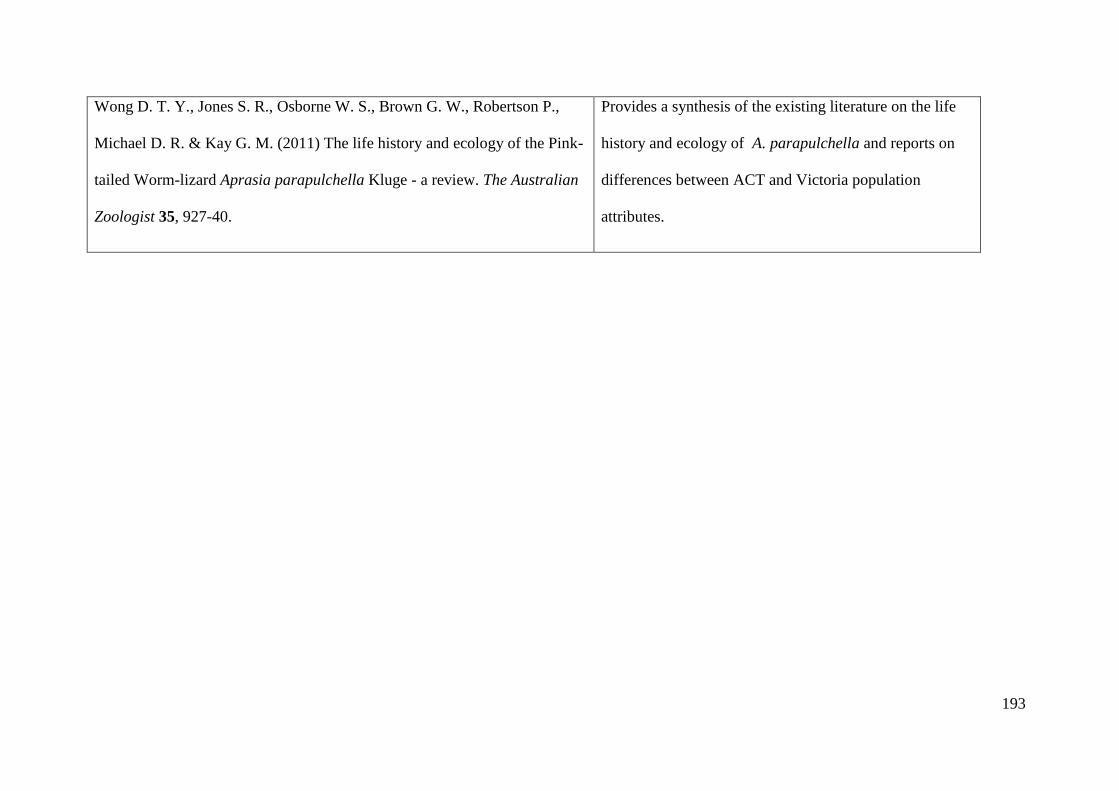
193
Wong D. T. Y., Jones S. R., Osborne W. S., Brown G. W., Robertson P.,
Michael D. R. & Kay G. M. (2011) The life history and ecology of the Pink-
tailed Worm-lizard Aprasia parapulchella Kluge - a review. The Australian
Zoologist 35, 927-40.
Provides a synthesis of the existing literature on the life
history and ecology of A. parapulchella and reports on
differences between ACT and Victoria population
attributes.

194
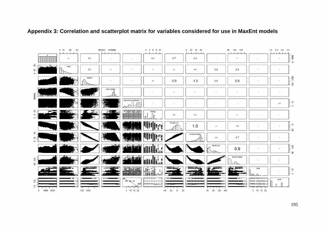
195
Appendix 3: Correlation and scatterplot matrix for variables considered for use in MaxEnt models

196
197
Appendix 4: Maxent output
N.B. “Myrecl” refers to the agricultural modification variable
This page summarizes the results of 10-fold cross-validation for Aprasia_parapulchella, created Tue Apr 09 17:24:07 EST 2013 using Maxent
version 3.3.3e. The individual models are here: [0] [1] [2] [3] [4] [5] [6] [7] [8] [9]
Analysis of omission/commission
The following picture shows the test omission rate and predicted area as a function of the cumulative threshold, averaged over the replicate runs.
The omission rate should be close to the predicted omission, because of the definition of the cumulative threshold.
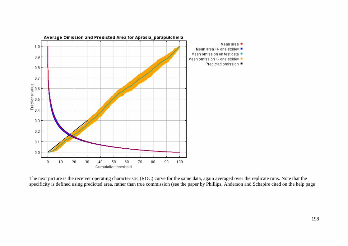
198
The next picture is the receiver operating characteristic (ROC) curve for the same data, again averaged over the replicate runs. Note that the
specificity is defined using predicted area, rather than true commission (see the paper by Phillips, Anderson and Schapire cited on the help page
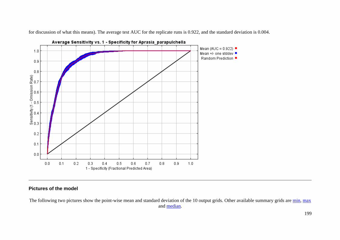
199
for discussion of what this means). The average test AUC for the replicate runs is 0.922, and the standard deviation is 0.004.
Pictures of the model
The following two pictures show the point-wise mean and standard deviation of the 10 output grids. Other available summary grids are min, max
and median.
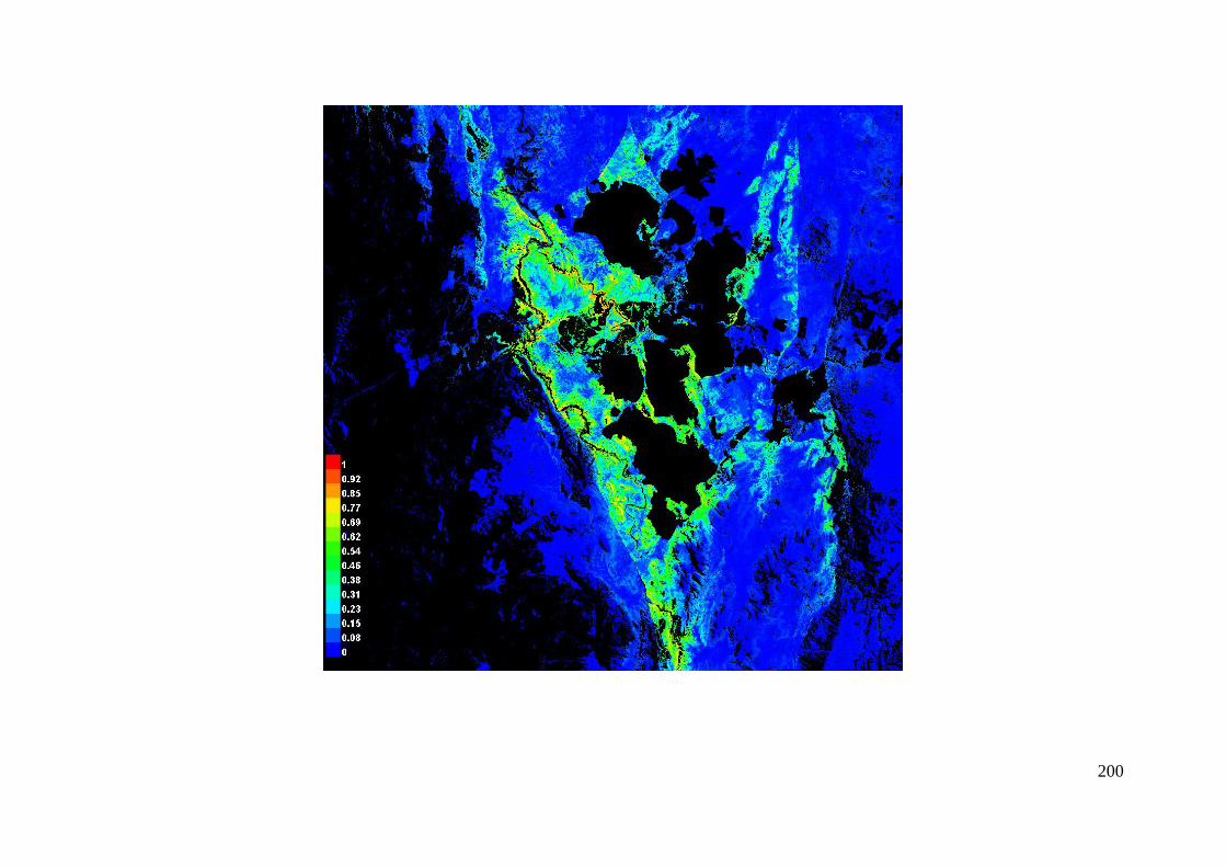
200
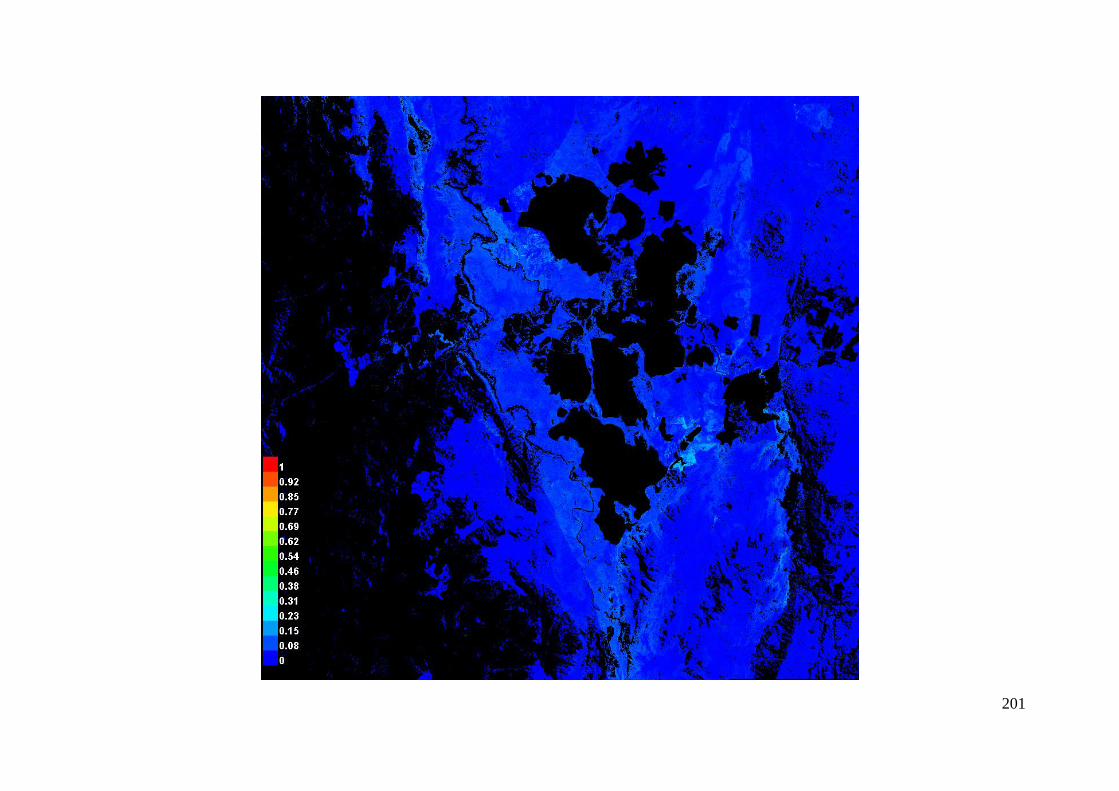
201
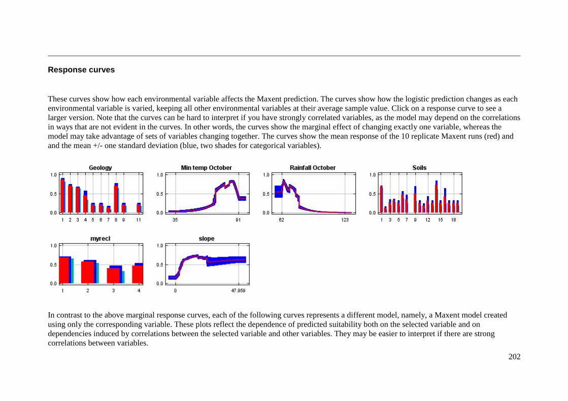
202
Response curves
These curves show how each environmental variable affects the Maxent prediction. The curves show how the logistic prediction changes as each
environmental variable is varied, keeping all other environmental variables at their average sample value. Click on a response curve to see a
larger version. Note that the curves can be hard to interpret if you have strongly correlated variables, as the model may depend on the correlations
in ways that are not evident in the curves. In other words, the curves show the marginal effect of changing exactly one variable, whereas the
model may take advantage of sets of variables changing together. The curves show the mean response of the 10 replicate Maxent runs (red) and
and the mean +/- one standard deviation (blue, two shades for categorical variables).
In contrast to the above marginal response curves, each of the following curves represents a different model, namely, a Maxent model created
using only the corresponding variable. These plots reflect the dependence of predicted suitability both on the selected variable and on
dependencies induced by correlations between the selected variable and other variables. They may be easier to interpret if there are strong
correlations between variables.
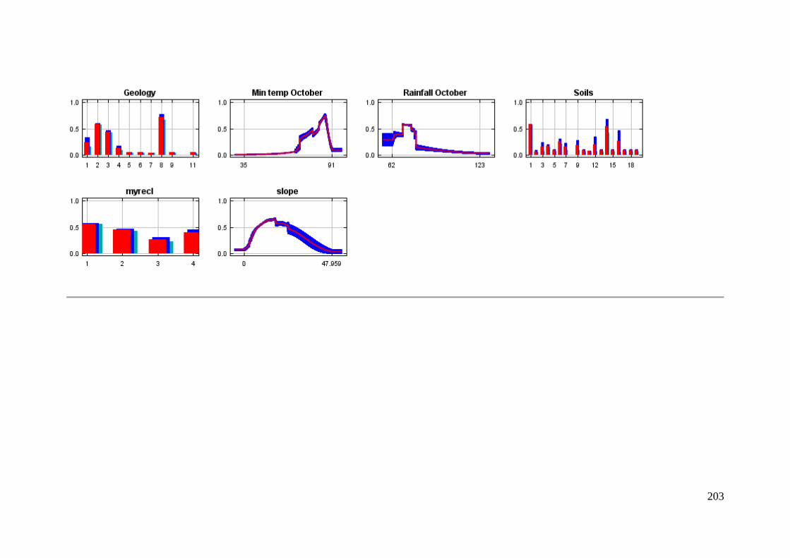
203
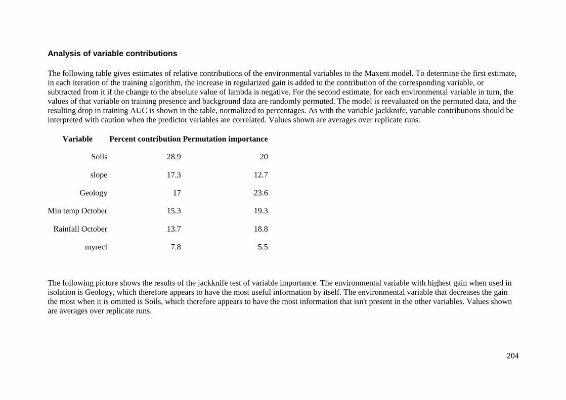
204
Analysis of variable contributions
The following table gives estimates of relative contributions of the environmental variables to the Maxent model. To determine the first estimate,
in each iteration of the training algorithm, the increase in regularized gain is added to the contribution of the corresponding variable, or
subtracted from it if the change to the absolute value of lambda is negative. For the second estimate, for each environmental variable in turn, the
values of that variable on training presence and background data are randomly permuted. The model is reevaluated on the permuted data, and the
resulting drop in training AUC is shown in the table, normalized to percentages. As with the variable jackknife, variable contributions should be
interpreted with caution when the predictor variables are correlated. Values shown are averages over replicate runs.
Variable Percent contribution Permutation importance
Soils 28.9 20
slope 17.3 12.7
Geology 17 23.6
Min temp October 15.3 19.3
Rainfall October 13.7 18.8
myrecl 7.8 5.5
The following picture shows the results of the jackknife test of variable importance. The environmental variable with highest gain when used in
isolation is Geology, which therefore appears to have the most useful information by itself. The environmental variable that decreases the gain
the most when it is omitted is Soils, which therefore appears to have the most information that isn't present in the other variables. Values shown
are averages over replicate runs.
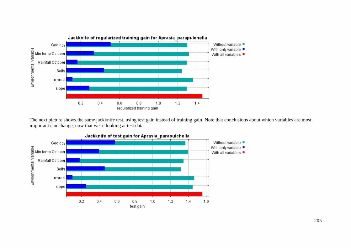
205
The next picture shows the same jackknife test, using test gain instead of training gain. Note that conclusions about which variables are most
important can change, now that we're looking at test data.
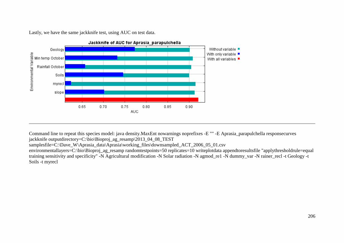
206
Lastly, we have the same jackknife test, using AUC on test data.
Command line to repeat this species model: java density.MaxEnt nowarnings noprefixes -E "" -E Aprasia_parapulchella responsecurves
jackknife outputdirectory=C:\bio\Bioproj_ag_resamp\2013_04_08_TEST
samplesfile=C:\Dave_W\Aprasia_data\Aprasia\working_files\downsampled_ACT_2006_05_01.csv
environmentallayers=C:\bio\Bioproj_ag_resamp randomtestpoints=50 replicates=10 writeplotdata appendtoresultsfile "applythresholdrule=equal
training sensitivity and specificity" -N Agricultural modification -N Solar radiation -N agmod_re1 -N dummy_var -N rainer_recl -t Geology -t
Soils -t myrecl
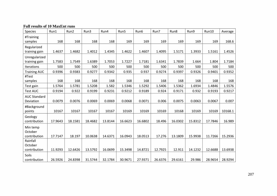
207
Full results of 10 MaxEnt runs
Species Run1 Run2 Run3 Run4 Run5 Run6 Run7 Run8 Run9 Run10 Average
#Training samples 168 168 168 168 169 169 169 169 169 169 168.6
Regularized training gain 1.4637 1.4682 1.4012 1.4345 1.4622 1.4607 1.4095 1.5171 1.3933 1.5161 1.4526
Unregularized training gain 1.7583 1.7549 1.6389 1.7053 1.7227 1.7181 1.6341 1.7839 1.664 1.804 1.7184
Iterations 500 500 500 500 500 500 500 500 500 500 500
Training AUC 0.9396 0.9383 0.9277 0.9342 0.935 0.937 0.9274 0.9397 0.9326 0.9401 0.9352
#Test samples 168 168 168 168 168 168 168 168 168 168 168
Test gain 1.5764 1.5781 1.5208 1.582 1.5346 1.5292 1.5406 1.5362 1.6934 1.4846 1.5576
Test AUC 0.9194 0.922 0.9199 0.9231 0.9212 0.9189 0.924 0.9171 0.932 0.9193 0.9217
AUC Standard Deviation 0.0079 0.0076 0.0069 0.0069 0.0068 0.0071 0.006 0.0075 0.0063 0.0067 0.007
#Background points 10167 10167 10167 10167 10169 10169 10169 10168 10169 10169 10168.1
Geology contribution 17.9643 18.1581 18.4682 13.8144 16.6623 16.6802 18.496 16.0302 15.8312 17.7846 16.989
Min temp October contribution 17.7147 18.197 10.0638 14.6371 16.0943 18.0513 17.276 13.1809 15.9938 11.7266 15.2936
Rainfall October contribution 11.9293 12.6426 13.5792 16.0699 15.3498 14.8721 12.7925 12.911 14.1232 12.6688 13.6938
Soils contribution 26.5926 24.8398 31.5744 32.1784 30.9671 27.9371 26.6376 29.6161 29.986 28.9654 28.9294
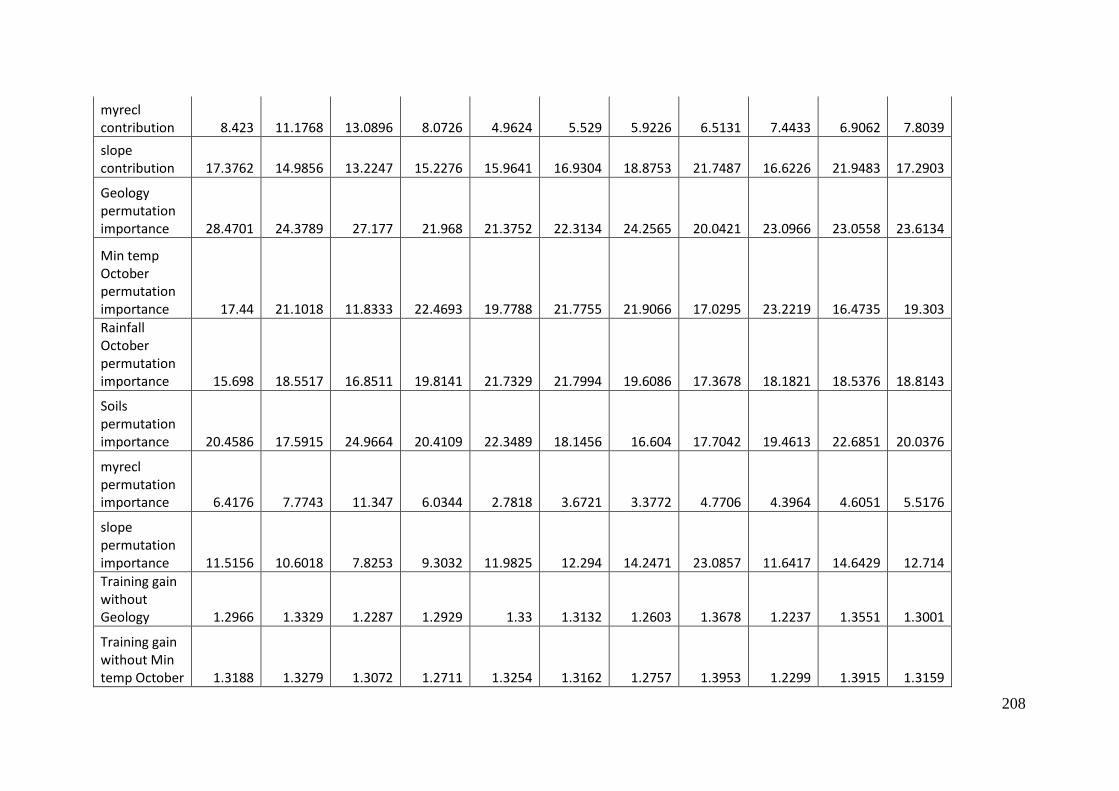
208
myrecl contribution 8.423 11.1768 13.0896 8.0726 4.9624 5.529 5.9226 6.5131 7.4433 6.9062 7.8039
slope contribution 17.3762 14.9856 13.2247 15.2276 15.9641 16.9304 18.8753 21.7487 16.6226 21.9483 17.2903
Geology permutation importance 28.4701 24.3789 27.177 21.968 21.3752 22.3134 24.2565 20.0421 23.0966 23.0558 23.6134
Min temp October permutation importance 17.44 21.1018 11.8333 22.4693 19.7788 21.7755 21.9066 17.0295 23.2219 16.4735 19.303
Rainfall October permutation importance 15.698 18.5517 16.8511 19.8141 21.7329 21.7994 19.6086 17.3678 18.1821 18.5376 18.8143
Soils permutation importance 20.4586 17.5915 24.9664 20.4109 22.3489 18.1456 16.604 17.7042 19.4613 22.6851 20.0376
myrecl permutation importance 6.4176 7.7743 11.347 6.0344 2.7818 3.6721 3.3772 4.7706 4.3964 4.6051 5.5176
slope permutation importance 11.5156 10.6018 7.8253 9.3032 11.9825 12.294 14.2471 23.0857 11.6417 14.6429 12.714
Training gain without Geology 1.2966 1.3329 1.2287 1.2929 1.33 1.3132 1.2603 1.3678 1.2237 1.3551 1.3001
Training gain without Min temp October 1.3188 1.3279 1.3072 1.2711 1.3254 1.3162 1.2757 1.3953 1.2299 1.3915 1.3159
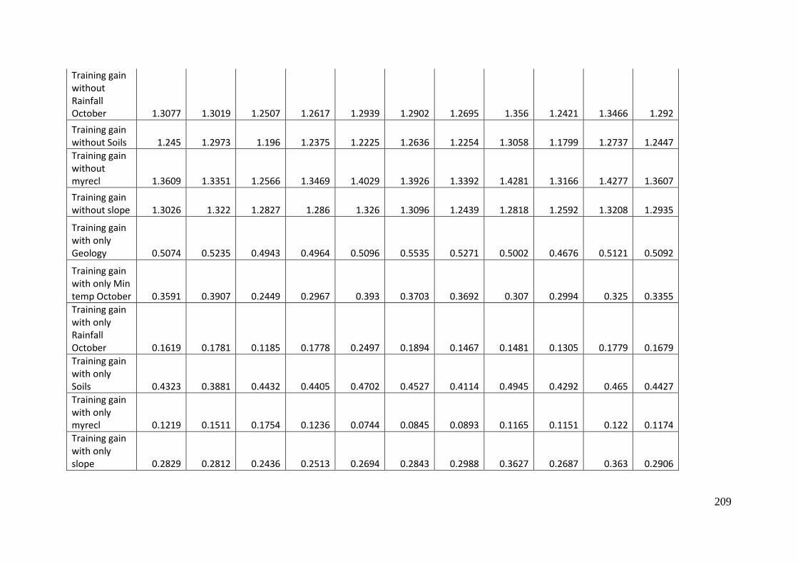
209
Training gain without Rainfall October 1.3077 1.3019 1.2507 1.2617 1.2939 1.2902 1.2695 1.356 1.2421 1.3466 1.292
Training gain without Soils 1.245 1.2973 1.196 1.2375 1.2225 1.2636 1.2254 1.3058 1.1799 1.2737 1.2447
Training gain without myrecl 1.3609 1.3351 1.2566 1.3469 1.4029 1.3926 1.3392 1.4281 1.3166 1.4277 1.3607
Training gain without slope 1.3026 1.322 1.2827 1.286 1.326 1.3096 1.2439 1.2818 1.2592 1.3208 1.2935
Training gain with only Geology 0.5074 0.5235 0.4943 0.4964 0.5096 0.5535 0.5271 0.5002 0.4676 0.5121 0.5092
Training gain with only Min temp October 0.3591 0.3907 0.2449 0.2967 0.393 0.3703 0.3692 0.307 0.2994 0.325 0.3355
Training gain with only Rainfall October 0.1619 0.1781 0.1185 0.1778 0.2497 0.1894 0.1467 0.1481 0.1305 0.1779 0.1679
Training gain with only Soils 0.4323 0.3881 0.4432 0.4405 0.4702 0.4527 0.4114 0.4945 0.4292 0.465 0.4427
Training gain with only myrecl 0.1219 0.1511 0.1754 0.1236 0.0744 0.0845 0.0893 0.1165 0.1151 0.122 0.1174
Training gain with only slope 0.2829 0.2812 0.2436 0.2513 0.2694 0.2843 0.2988 0.3627 0.2687 0.363 0.2906
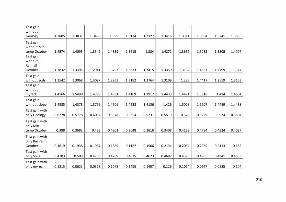
210
Test gain without Geology 1.3805 1.3837 1.3468 1.399 1.3174 1.3327 1.3416 1.3311 1.5384 1.3241 1.3695
Test gain without Min temp October 1.4574 1.4095 1.3549 1.4339 1.3215 1.384 1.4272 1.3652 1.5233 1.3305 1.4007
Test gain without Rainfall October 1.3832 1.3395 1.2941 1.3797 1.3333 1.3415 1.3359 1.3162 1.4667 1.2799 1.347
Test gain without Soils 1.3542 1.3068 1.3097 1.2963 1.3182 1.2764 1.3109 1.283 1.4417 1.2559 1.3153
Test gain without myrecl 1.4566 1.5498 1.4796 1.4931 1.4169 1.3917 1.4433 1.4471 1.5918 1.414 1.4684
Test gain without slope 1.4585 1.4378 1.3796 1.4506 1.4238 1.4136 1.426 1.5028 1.5507 1.4449 1.4488
Test gain with only Geology 0.6278 0.5778 0.6054 0.5578 0.5354 0.5231 0.5519 0.628 0.6229 0.574 0.5804
Test gain with only Min temp October 0.388 0.3683 0.458 0.4201 0.3648 0.3616 0.3408 0.4138 0.4794 0.4324 0.4027
Test gain with only Rainfall October 0.1619 0.1938 0.1967 0.1689 0.1127 0.1506 0.2134 0.2064 0.2339 0.2113 0.185
Test gain with only Soils 0.4703 0.509 0.4203 0.4789 0.4015 0.4623 0.4687 0.4398 0.4985 0.4841 0.4633
Test gain with only myrecl 0.1315 0.0623 0.0318 0.1078 0.1495 0.1497 0.126 0.1014 0.0967 0.0835 0.104
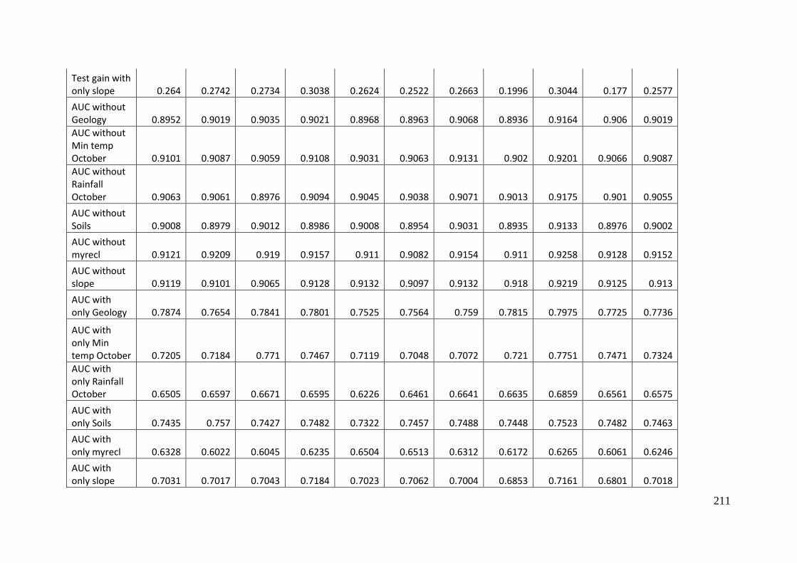
211
Test gain with only slope 0.264 0.2742 0.2734 0.3038 0.2624 0.2522 0.2663 0.1996 0.3044 0.177 0.2577
AUC without Geology 0.8952 0.9019 0.9035 0.9021 0.8968 0.8963 0.9068 0.8936 0.9164 0.906 0.9019
AUC without Min temp October 0.9101 0.9087 0.9059 0.9108 0.9031 0.9063 0.9131 0.902 0.9201 0.9066 0.9087
AUC without Rainfall October 0.9063 0.9061 0.8976 0.9094 0.9045 0.9038 0.9071 0.9013 0.9175 0.901 0.9055
AUC without Soils 0.9008 0.8979 0.9012 0.8986 0.9008 0.8954 0.9031 0.8935 0.9133 0.8976 0.9002
AUC without myrecl 0.9121 0.9209 0.919 0.9157 0.911 0.9082 0.9154 0.911 0.9258 0.9128 0.9152
AUC without slope 0.9119 0.9101 0.9065 0.9128 0.9132 0.9097 0.9132 0.918 0.9219 0.9125 0.913
AUC with only Geology 0.7874 0.7654 0.7841 0.7801 0.7525 0.7564 0.759 0.7815 0.7975 0.7725 0.7736
AUC with only Min temp October 0.7205 0.7184 0.771 0.7467 0.7119 0.7048 0.7072 0.721 0.7751 0.7471 0.7324
AUC with only Rainfall October 0.6505 0.6597 0.6671 0.6595 0.6226 0.6461 0.6641 0.6635 0.6859 0.6561 0.6575
AUC with only Soils 0.7435 0.757 0.7427 0.7482 0.7322 0.7457 0.7488 0.7448 0.7523 0.7482 0.7463
AUC with only myrecl 0.6328 0.6022 0.6045 0.6235 0.6504 0.6513 0.6312 0.6172 0.6265 0.6061 0.6246
AUC with only slope 0.7031 0.7017 0.7043 0.7184 0.7023 0.7062 0.7004 0.6853 0.7161 0.6801 0.7018
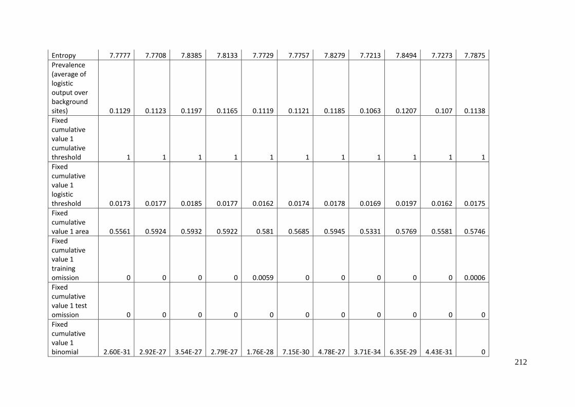
212
Entropy 7.7777 7.7708 7.8385 7.8133 7.7729 7.7757 7.8279 7.7213 7.8494 7.7273 7.7875
Prevalence (average of logistic output over background sites) 0.1129 0.1123 0.1197 0.1165 0.1119 0.1121 0.1185 0.1063 0.1207 0.107 0.1138
Fixed cumulative value 1 cumulative threshold 1 1 1 1 1 1 1 1 1 1 1
Fixed cumulative value 1 logistic threshold 0.0173 0.0177 0.0185 0.0177 0.0162 0.0174 0.0178 0.0169 0.0197 0.0162 0.0175
Fixed cumulative value 1 area 0.5561 0.5924 0.5932 0.5922 0.581 0.5685 0.5945 0.5331 0.5769 0.5581 0.5746
Fixed cumulative value 1 training omission 0 0 0 0 0.0059 0 0 0 0 0 0.0006
Fixed cumulative value 1 test omission 0 0 0 0 0 0 0 0 0 0 0
Fixed cumulative value 1 binomial 2.60E-31 2.92E-27 3.54E-27 2.79E-27 1.76E-28 7.15E-30 4.78E-27 3.71E-34 6.35E-29 4.43E-31 0
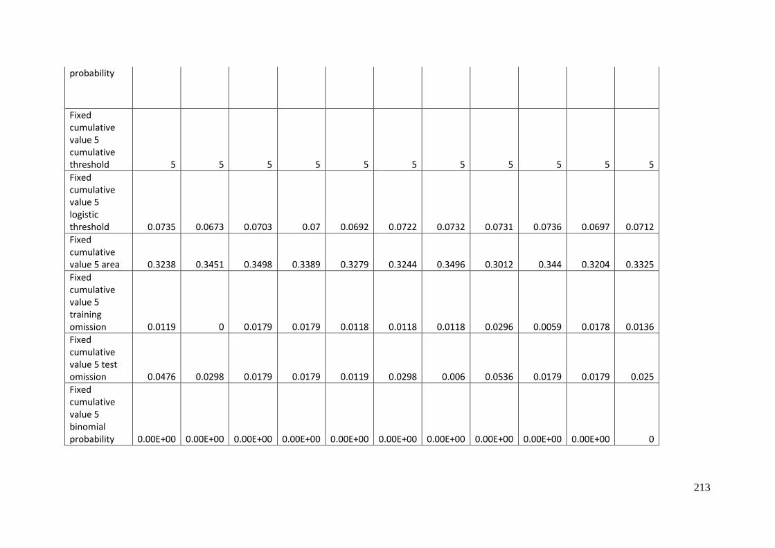
213
probability
Fixed cumulative value 5 cumulative threshold 5 5 5 5 5 5 5 5 5 5 5
Fixed cumulative value 5 logistic threshold 0.0735 0.0673 0.0703 0.07 0.0692 0.0722 0.0732 0.0731 0.0736 0.0697 0.0712
Fixed cumulative value 5 area 0.3238 0.3451 0.3498 0.3389 0.3279 0.3244 0.3496 0.3012 0.344 0.3204 0.3325
Fixed cumulative value 5 training omission 0.0119 0 0.0179 0.0179 0.0118 0.0118 0.0118 0.0296 0.0059 0.0178 0.0136
Fixed cumulative value 5 test omission 0.0476 0.0298 0.0179 0.0179 0.0119 0.0298 0.006 0.0536 0.0179 0.0179 0.025
Fixed cumulative value 5 binomial probability 0.00E+00 0.00E+00 0.00E+00 0.00E+00 0.00E+00 0.00E+00 0.00E+00 0.00E+00 0.00E+00 0.00E+00 0
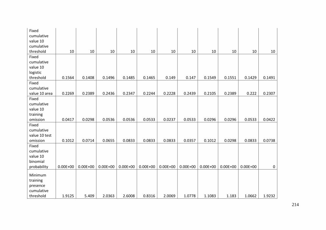
214
Fixed cumulative value 10 cumulative threshold 10 10 10 10 10 10 10 10 10 10 10
Fixed cumulative value 10 logistic threshold 0.1564 0.1408 0.1496 0.1485 0.1465 0.149 0.147 0.1549 0.1551 0.1429 0.1491
Fixed cumulative value 10 area 0.2269 0.2389 0.2436 0.2347 0.2244 0.2228 0.2439 0.2105 0.2389 0.222 0.2307
Fixed cumulative value 10 training omission 0.0417 0.0298 0.0536 0.0536 0.0533 0.0237 0.0533 0.0296 0.0296 0.0533 0.0422
Fixed cumulative value 10 test omission 0.1012 0.0714 0.0655 0.0833 0.0833 0.0833 0.0357 0.1012 0.0298 0.0833 0.0738
Fixed cumulative value 10 binomial probability 0.00E+00 0.00E+00 0.00E+00 0.00E+00 0.00E+00 0.00E+00 0.00E+00 0.00E+00 0.00E+00 0.00E+00 0
Minimum training presence cumulative threshold 1.9125 5.409 2.0363 2.6008 0.8316 2.0069 1.0778 1.1083 1.183 1.0662 1.9232
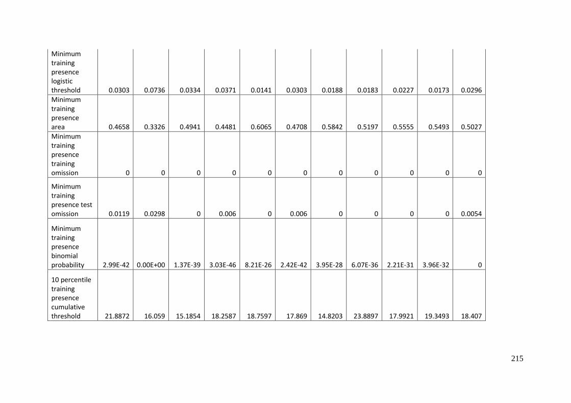
215
Minimum training presence logistic threshold 0.0303 0.0736 0.0334 0.0371 0.0141 0.0303 0.0188 0.0183 0.0227 0.0173 0.0296
Minimum training presence area 0.4658 0.3326 0.4941 0.4481 0.6065 0.4708 0.5842 0.5197 0.5555 0.5493 0.5027
Minimum training presence training omission 0 0 0 0 0 0 0 0 0 0 0
Minimum training presence test omission 0.0119 0.0298 0 0.006 0 0.006 0 0 0 0 0.0054
Minimum training presence binomial probability 2.99E-42 0.00E+00 1.37E-39 3.03E-46 8.21E-26 2.42E-42 3.95E-28 6.07E-36 2.21E-31 3.96E-32 0
10 percentile training presence cumulative threshold 21.8872 16.059 15.1854 18.2587 18.7597 17.869 14.8203 23.8897 17.9921 19.3493 18.407
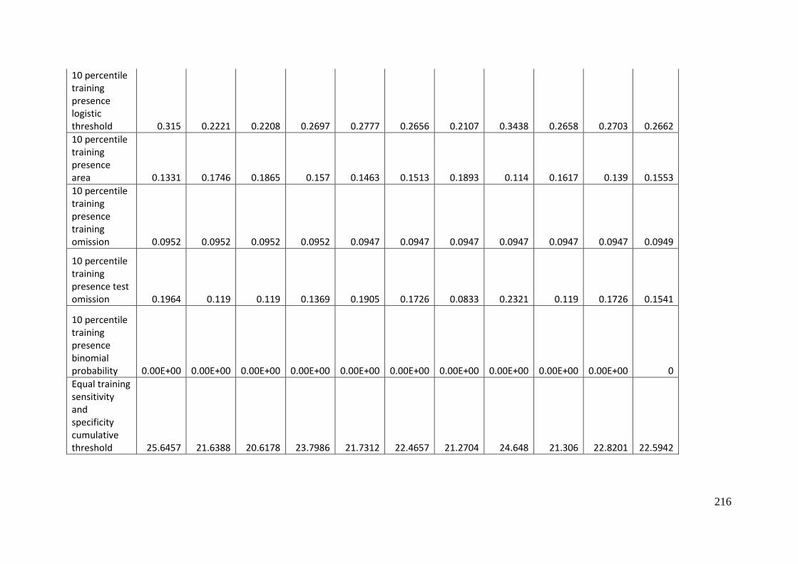
216
10 percentile training presence logistic threshold 0.315 0.2221 0.2208 0.2697 0.2777 0.2656 0.2107 0.3438 0.2658 0.2703 0.2662
10 percentile training presence area 0.1331 0.1746 0.1865 0.157 0.1463 0.1513 0.1893 0.114 0.1617 0.139 0.1553
10 percentile training presence training omission 0.0952 0.0952 0.0952 0.0952 0.0947 0.0947 0.0947 0.0947 0.0947 0.0947 0.0949
10 percentile training presence test omission 0.1964 0.119 0.119 0.1369 0.1905 0.1726 0.0833 0.2321 0.119 0.1726 0.1541
10 percentile training presence binomial probability 0.00E+00 0.00E+00 0.00E+00 0.00E+00 0.00E+00 0.00E+00 0.00E+00 0.00E+00 0.00E+00 0.00E+00 0
Equal training sensitivity and specificity cumulative threshold 25.6457 21.6388 20.6178 23.7986 21.7312 22.4657 21.2704 24.648 21.306 22.8201 22.5942
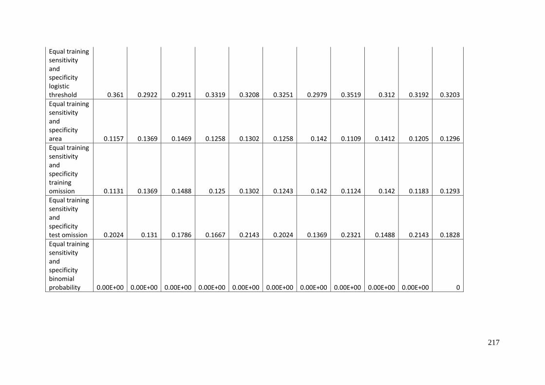
217
Equal training sensitivity and specificity logistic threshold 0.361 0.2922 0.2911 0.3319 0.3208 0.3251 0.2979 0.3519 0.312 0.3192 0.3203
Equal training sensitivity and specificity area 0.1157 0.1369 0.1469 0.1258 0.1302 0.1258 0.142 0.1109 0.1412 0.1205 0.1296
Equal training sensitivity and specificity training omission 0.1131 0.1369 0.1488 0.125 0.1302 0.1243 0.142 0.1124 0.142 0.1183 0.1293
Equal training sensitivity and specificity test omission 0.2024 0.131 0.1786 0.1667 0.2143 0.2024 0.1369 0.2321 0.1488 0.2143 0.1828
Equal training sensitivity and specificity binomial probability 0.00E+00 0.00E+00 0.00E+00 0.00E+00 0.00E+00 0.00E+00 0.00E+00 0.00E+00 0.00E+00 0.00E+00 0
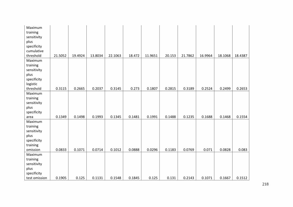
218
Maximum training sensitivity plus specificity cumulative threshold 21.5052 19.4924 13.8034 22.1063 18.472 11.9651 20.153 21.7862 16.9964 18.1068 18.4387
Maximum training sensitivity plus specificity logistic threshold 0.3115 0.2665 0.2037 0.3145 0.273 0.1807 0.2815 0.3189 0.2524 0.2499 0.2653
Maximum training sensitivity plus specificity area 0.1349 0.1498 0.1993 0.1345 0.1481 0.1991 0.1488 0.1235 0.1688 0.1468 0.1554
Maximum training sensitivity plus specificity training omission 0.0833 0.1071 0.0714 0.1012 0.0888 0.0296 0.1183 0.0769 0.071 0.0828 0.083
Maximum training sensitivity plus specificity test omission 0.1905 0.125 0.1131 0.1548 0.1845 0.125 0.131 0.2143 0.1071 0.1667 0.1512
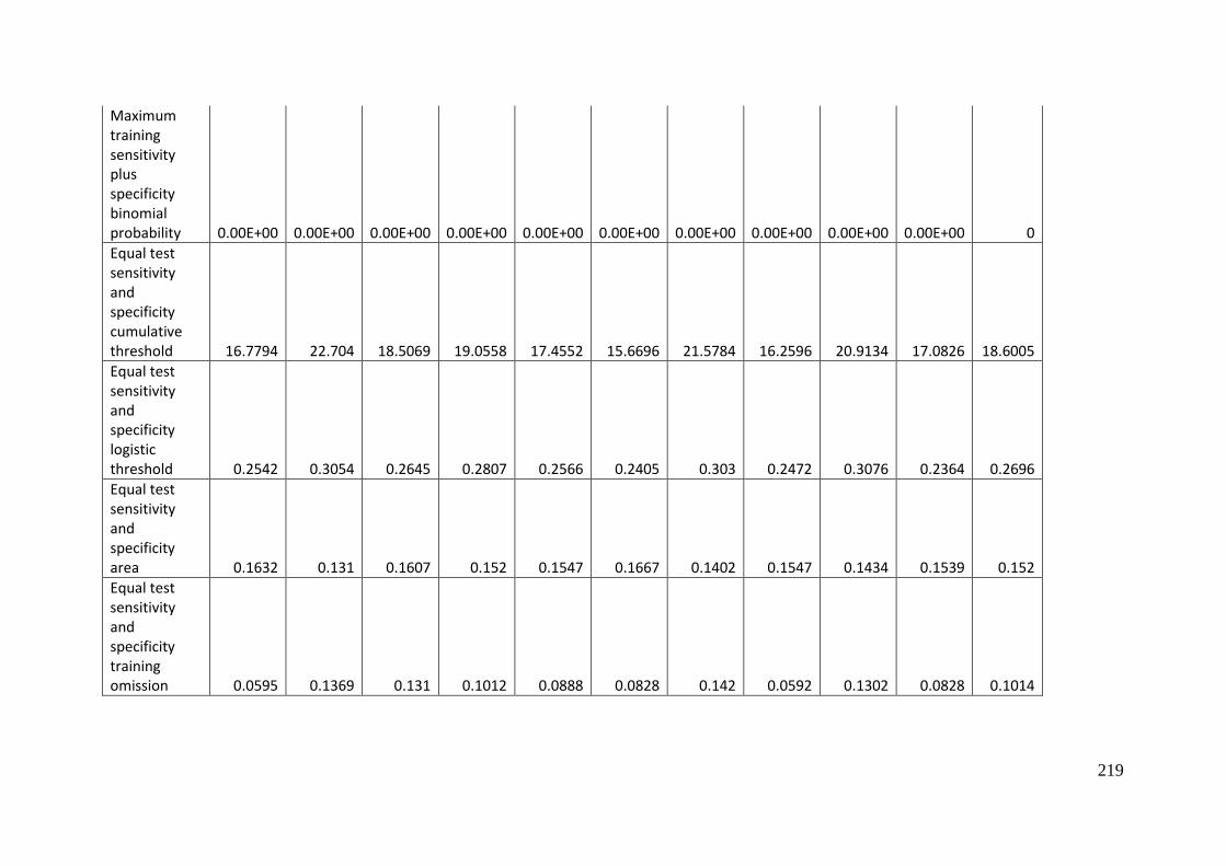
219
Maximum training sensitivity plus specificity binomial probability 0.00E+00 0.00E+00 0.00E+00 0.00E+00 0.00E+00 0.00E+00 0.00E+00 0.00E+00 0.00E+00 0.00E+00 0
Equal test sensitivity and specificity cumulative threshold 16.7794 22.704 18.5069 19.0558 17.4552 15.6696 21.5784 16.2596 20.9134 17.0826 18.6005
Equal test sensitivity and specificity logistic threshold 0.2542 0.3054 0.2645 0.2807 0.2566 0.2405 0.303 0.2472 0.3076 0.2364 0.2696
Equal test sensitivity and specificity area 0.1632 0.131 0.1607 0.152 0.1547 0.1667 0.1402 0.1547 0.1434 0.1539 0.152
Equal test sensitivity and specificity training omission 0.0595 0.1369 0.131 0.1012 0.0888 0.0828 0.142 0.0592 0.1302 0.0828 0.1014
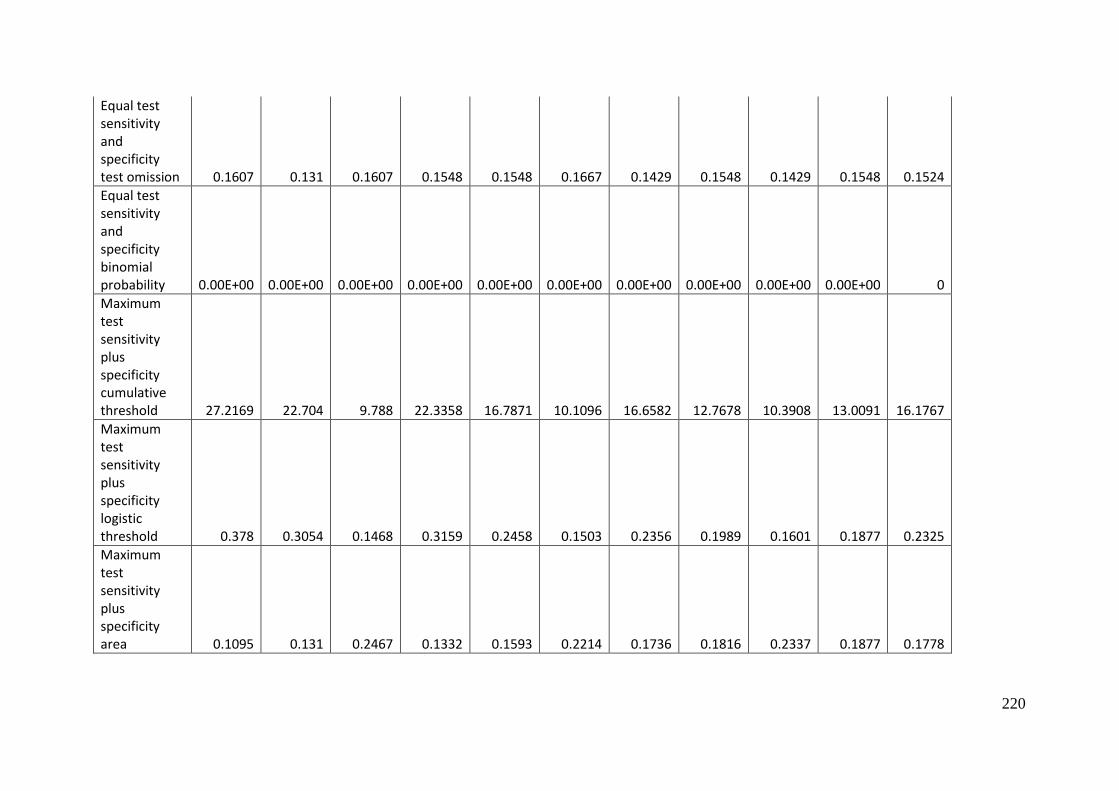
220
Equal test sensitivity and specificity test omission 0.1607 0.131 0.1607 0.1548 0.1548 0.1667 0.1429 0.1548 0.1429 0.1548 0.1524
Equal test sensitivity and specificity binomial probability 0.00E+00 0.00E+00 0.00E+00 0.00E+00 0.00E+00 0.00E+00 0.00E+00 0.00E+00 0.00E+00 0.00E+00 0
Maximum test sensitivity plus specificity cumulative threshold 27.2169 22.704 9.788 22.3358 16.7871 10.1096 16.6582 12.7678 10.3908 13.0091 16.1767
Maximum test sensitivity plus specificity logistic threshold 0.378 0.3054 0.1468 0.3159 0.2458 0.1503 0.2356 0.1989 0.1601 0.1877 0.2325
Maximum test sensitivity plus specificity area 0.1095 0.131 0.2467 0.1332 0.1593 0.2214 0.1736 0.1816 0.2337 0.1877 0.1778
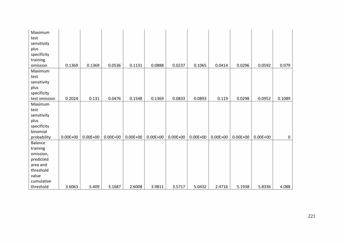
221
Maximum test sensitivity plus specificity training omission 0.1369 0.1369 0.0536 0.1131 0.0888 0.0237 0.1065 0.0414 0.0296 0.0592 0.079
Maximum test sensitivity plus specificity test omission 0.2024 0.131 0.0476 0.1548 0.1369 0.0833 0.0893 0.119 0.0298 0.0952 0.1089
Maximum test sensitivity plus specificity binomial probability 0.00E+00 0.00E+00 0.00E+00 0.00E+00 0.00E+00 0.00E+00 0.00E+00 0.00E+00 0.00E+00 0.00E+00 0
Balance training omission, predicted area and threshold value cumulative threshold 3.6063 5.409 3.1687 2.6008 3.9811 3.5717 5.0432 2.4716 5.1938 5.8336 4.088
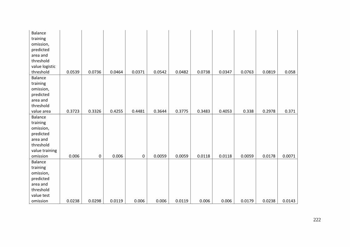
222
Balance training omission, predicted area and threshold value logistic threshold 0.0539 0.0736 0.0464 0.0371 0.0542 0.0482 0.0738 0.0347 0.0763 0.0819 0.058
Balance training omission, predicted area and threshold value area 0.3723 0.3326 0.4255 0.4481 0.3644 0.3775 0.3483 0.4053 0.338 0.2978 0.371
Balance training omission, predicted area and threshold value training omission 0.006 0 0.006 0 0.0059 0.0059 0.0118 0.0118 0.0059 0.0178 0.0071
Balance training omission, predicted area and threshold value test omission 0.0238 0.0298 0.0119 0.006 0.006 0.0119 0.006 0.006 0.0179 0.0238 0.0143
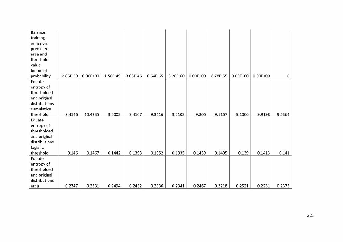
223
Balance training omission, predicted area and threshold value binomial probability 2.86E-59 0.00E+00 1.56E-49 3.03E-46 8.64E-65 3.26E-60 0.00E+00 8.78E-55 0.00E+00 0.00E+00 0
Equate entropy of thresholded and original distributions cumulative threshold 9.4146 10.4235 9.6003 9.4107 9.3616 9.2103 9.806 9.1167 9.1006 9.9198 9.5364
Equate entropy of thresholded and original distributions logistic threshold 0.146 0.1467 0.1442 0.1393 0.1352 0.1335 0.1439 0.1405 0.139 0.1413 0.141
Equate entropy of thresholded and original distributions area 0.2347 0.2331 0.2494 0.2432 0.2336 0.2341 0.2467 0.2218 0.2521 0.2231 0.2372
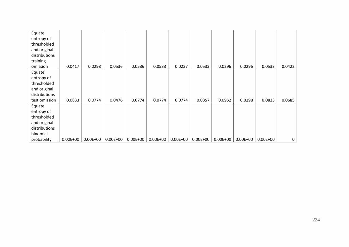
224
Equate entropy of thresholded and original distributions training omission 0.0417 0.0298 0.0536 0.0536 0.0533 0.0237 0.0533 0.0296 0.0296 0.0533 0.0422
Equate entropy of thresholded and original distributions test omission 0.0833 0.0774 0.0476 0.0774 0.0774 0.0774 0.0357 0.0952 0.0298 0.0833 0.0685
Equate entropy of thresholded and original distributions binomial probability 0.00E+00 0.00E+00 0.00E+00 0.00E+00 0.00E+00 0.00E+00 0.00E+00 0.00E+00 0.00E+00 0.00E+00 0
Appendix 5: Rehwinkel R. (2007) A method to assess grassy
ecosystem sites: using floristic information to assess a site's
quality. NSW Department of Environment and Climate Change,
Queanbeyan, NSW.
A Method to Assess Grassy Ecosystem Sites: Using floristic information to assess a site’s quality Rainer Rehwinkel
Senior Threatened Species Officer Biodiversity Conservation Section Climate Change & Environment Protection Group South Branch NSW Department of Environment and Climate Change
November 2007 (v.2)
A Method to Assess Grassy Ecosystem Sites: Using floristic information to assess a site’s quality R. Rehwinkel © DECC
2007
226
Table of Contents
INTRODUCTION 227
The significant species concept 227
Grassland assessment 227
Secondary grasslands 228
Other grassland values 228
Regionalisation 228
The floristic value score method 229
FIGURE 1. DECISION TREE FOR ASSESSING THE VEGETATION TYPE OF A GRASSY SITE 231
FIGURE 2. DECISION TREE FOR ASSESSING CONSERVATION VALUE OF A GRASSY SITE 232
ANALYSIS OF A SITE TO DETERMINE ITS “FLORISTIC VALUE SCORE” 233
HOW TO GATHER DATA: STRATIFICATION, SAMPLING EFFORT AND DATA COLLECTION 233
Stratification 233
Field method 233
Data collection 234
THE ANALYSIS OF DATA TO DERIVE A “FLORISTIC VALUE SCORE” 235
REPORTING 238
ACKNOWLEDGMENTS AND DISCLAIMER 239
REFERENCES 239
APPENDIX 1. LIST OF SPECIES OF THE MONARO SUB-REGION. 240
APPENDIX 2. LIST OF SPECIES OF THE EASTERN SUB-REGION. 242
APPENDIX 3. LIST OF SPECIES OF THE NORTH-WESTERN SUB-REGION. 244
APPENDIX 4. CALCULATION TABLE (FOR PHOTOCOPYING) 246
A Method to Assess Grassy Ecosystem Sites: Using floristic information to assess a site’s quality R. Rehwinkel © DECC
2007
227
A Method to Assess Grassy Ecosystem Sites: Using floristic information to assess a site’s quality Introduction This document presents a quantitative method that enables the assessment of the relative values of sites containing any of the communities within the grassy ecosystems found in the Southern Tablelands of NSW. This method can be used in the following vegetation types:
The grassy groundlayer of White Box Yellow Box Blakely’s Red Gum Woodland (Box-Gum Woodland), a listed endangered ecological community (EEC) under the NSW Threatened Species Conservation Act (1995);
Secondary grassland derived from Box-Gum Woodland EEC;
Native grassland that falls under the definitions of Natural Temperate Grassland of the Natural Temperate Grassland of the Southern Tablelands (NSW and ACT), a listed threatened ecological community under the Commonwealth’s Environmental Protection and Biodiversity Conservation Act (1999); and
The grassy groundlayers of Grassy Snow Gum Woodland and other regionally declining vegetation communities and the secondary grasslands derived from these.
The significant species concept This method has been developed using data collected in site surveys of grassy ecosystems throughout the Southern Tablelands in NSW and ACT since the early 1990’s (see Acknowledgments). The method is based upon the “significant species” concept, which relies on the application of a “significance score” to most of the roughly 650 species that have been recorded in grassy ecosystems within the region. Briefly, most grassy ecosystem species have been assigned a score based on their rarity in the regional data, with the rarest species assigned a score of 5, and the most common, a score of 1. A number of species, although apparently rare in the data, are thought to be “disturbance-tolerant”, “disturbance responding” or “increaser” species. This is based on observations and expert opinion. Increasers respond positively to various disturbances and are thus most commonly recorded in disturbed sites. Increaser species have been arbitrarily given a score of 1. However, not all increasers are scored 1. There is a limited subset of disturbance responders that retain their high scores, because, while responding to particular disturbance regimes (e.g. soil disturbance), they may not persist under others (e.g. grazing). Examples in this subset include Button Wrinklewort (Rutidosis leptorrhynchoides), Hoary Sunray (Leucochrysum albicans) and Aromatic Peppercress (Lepidium hyssopifolium), all of which are listed as endangered in one or more jurisdictions.
This method relies on three groupings of species, referred to as: 1. Common or increaser species, which do not add much to the value of a site; these
have a significance score of 1; 2. “Indicator species, level 1”, which indicate that the site has value; and 3. “Indicator species, level 2”, which are the highly significant species; these are the
rarest of the grassy ecosystems species and have the highest significance scores.
The indicator species are also sometimes referred to as “grazing-intolerant” or “declining” species. It is thought that these species are rare for two reasons:
1. Some species have always been rare, particularly some species which are restricted in distribution; and
2. Many species are thought to have undergone serious declines since European settlement, from disturbances such as over-grazing and application of fertilisers. This is based upon analysis of the data and observations of where such species still occur; the sites with the greatest concentrations of significant species today include cemeteries, road and rail reserves and sites such as travelling stock reserves and private land sites where grazing has been either non-existent or light (e.g. Prober & Thiele, 1993; Lunt, 1995; McIntyre, McIvor & Heard, 2002; R. Rehwinkel, unpublished data).
Grassland assessment Grasslands have been traditionally difficult to assess because of their inherent variability. Before the European settlement of the Southern Tablelands, there were extensive grassy
A Method to Assess Grassy Ecosystem Sites: Using floristic information to assess a site’s quality R. Rehwinkel © DECC
2007
228
plains as well as smaller areas of grassland within a mosaic of woodlands (Thomas et al. 2000). Now relatively few remnants of these communities remain in a state that resembles the former grasslands. The same applies to grassy woodland communities (Thomas et al. 2000). However, in some regions, large areas of grassland are retained that are variously described as native pasture, and degraded or highly modified native grassland (Environment ACT, 2005; Langford et al. 2004). Across the Southern Tablelands, these areas vary in their extent, according to the climate, soil types and land use history.
Within any particular area, remnant grasslands and grassy woodlands exist along a continuum. At one end of this continuum, there are the rare sites that retain a high degree of integrity (i.e. very high floristic diversity, varied structure that provides habitat for a diverse fauna, and low or absent exotic plant cover). At the other end of this continuum are the more extensive areas of native pasture, and degraded or highly modified grassland. Such grasslands usually have very low native plant diversity, limited fauna habitat values, and often a high cover and diversity of exotic plant species, many of which are either introduced pasture species or agricultural and environmental weeds.
Because grassland and woodland sites now exist in a continuum, with sites exhibiting all states between those with the highest integrity to those that are severely degraded, it has traditionally been difficult to draw a line between sites that could be described as of high flora conservation value and those which are less important for conservation. It was found necessary to develop guidelines to determine which sites should be considered to be of conservation significance. The approach presented in these guidelines provides a transparent and repeatable process that can be applied across the NSW portion of the Southern Tablelands to determine the conservation significance of any grassland and woodland site assessed. The value of these guidelines for use in the ACT needs to be further tested, though the general principles are likely to apply there too.
Secondary grasslands Grasslands vary in their origin. This has the potential to create confusion, especially in parts of the landscape that are heavily cleared and it is difficult to determine whether a site is natural or “secondary” grassland (i.e. grassland that results in the clearing of trees in a woodland or forest). This document provides guidance in those cases where it is difficult to determine whether a grassland is natural or secondary.
Other grassland values The method presented in this document provides a way to assess grasslands and woodland groundlayers primarily on their floristic values. It is important to remember that other values exist, including:
Presence of fauna, particularly of threatened species;
Presence of habitat attributes, including the presence of rocky outcrops, loose surface rocks, exposed banks, course woody debris, tree hollows, standing dead timber, or structural elements provided by certain plant species such as shrubs and tall tussocks;
Extent or lack of cover of weed species, with sites with a high cover of perennial weed species generally of lesser value than those without weeds;
The size of the remnant, with larger sites clearly being of greater value than smaller sites;
The shape of the remnant, with a blocky or circular shaped site being considered to be more valuable than a long, narrow site; and
The site’s connectivity, with a site that adjoins, is adjacent to, or nearby to other sites of the same or even different vegetation types being intrinsically more valuable than an isolated site.
Sites thus need to be assessed for their other values, alongside the floristic values that can be assessed using this document.
Regionalisation This document divides the Southern Tablelands into four broad regions, as recognised in the National Recovery Plan for Natural Temperate Grassland of the Southern Tablelands (NSW & ACT)(Environment ACT, 2005, p. 13). These regions are:
A Method to Assess Grassy Ecosystem Sites: Using floristic information to assess a site’s quality R. Rehwinkel © DECC
2007
229
Monaro sub-region: from the Victorian border to the south-eastern border of the ACT and west to Kosciuszko National Park (includes Michelago, Cooma, Jindabyne and Bombala);
Eastern sub-region: the area east and north-east of the ACT covering the upper Wollondilly River, upper Shoalhaven River and Lake George catchments (includes Collector, Bungendore, Taralga, Crookwell, Goulburn and Braidwood);
North-western sub-region: the area north of the ACT, covering part of the Murrumbidgee and Lachlan River catchments (includes Boorowa, Crookwell, Yass, Gunning, Gundaroo and Queanbeyan); and
ACT: an area defined by the political boundary. Each of these sub-regions have different floras, manifested in the differences in the forb, shrub and tree species that are found in each sub-region. Additionally, each region has distinctive land-use patterns. Much of the Monaro sub-region retains its native grassland and substantial areas of woodland also remain, though only relatively small areas retain moderate to high floristic values. In contrast, while there were formerly substantial areas of natural grassland and box-gum woodland in the North-western sub-region, very few areas remain, as grasslands and woodlands in this area have suffered extensive modification for “pasture improvement” and cropping. An intermediate picture emerges in the Eastern sub-region, where, while there has been extensive pasture modification and cropping, some large remnants of high value have been retained. The ACT has similarly lost much of its grassland and woodland to urban development, as well as to pasture modification and cropping, though, significantly, large areas have now been secured for conservation in this territory.
As stated previously, while the significance scores for all species were derived using data from both NSW and ACT, this assessment method has not been tested specifically on ACT sites. However, sites in the ACT could in all likelihood be assessed for their relative value using this method by applying the criteria and lists derived for the North-western sub-region (see The analysis of data to derive a Significance Score, below), being mindful of the fact that the ACT Government has developed specific methods to assess whether sites qualify as native grassland and woodland communities within the ACT (ACT Government, 2004; ACT Government, 2005).
The floristic and land-use differences expressed between the regions are reflected in the slight differences in species lists used for assessment in this method (see Appendices 1, 2 & 3.).
The floristic value score method
The method set out in this document allows assessment to be made of the following:
1. Is the site a natural or secondary grassland?; 2. If it is a natural grassland, does it have values consistent with those defined for the
Natural Temperate Grassland EEC?; and 3. Regardless of which type of grassland or woodland groundlayer present, what is its
floristic value?
Recently, an analysis has been undertaken to define the various associations found within natural grassland communities of the Southern Tablelands. Eight clearly defined associations have been identified using PATN analysis of a large dataset (Rehwinkel, in prep.). Previous analyses in the region (Thomas et al., 2000; Tindall et al., 2006) have defined a number of grassy woodland communities within the region. The method presented in this document treats all grassland and woodland communities of the Southern Tablelands as a single entity, with no reference to the differences found between the variously identified associations. To a large degree, however, the regional rarity of some of the forb, shrub and tree species in the regional data used to develop this method parallels the indicator species that help define some of the previously defined grassland or woodland associations. In reality, this method treats grassy ecosystems as three entities, as defined by the geographic boundaries defined in Environment ACT (2005). However, one of the associations of the natural grassland types is recognised in this method, namely the River Tussock Grassland dominated by Poa labillardierii that occurs along drainage lines or on flats associated with drainage features. Sites of this association in good condition are particularly rare and are often low in forb diversity. Most sites have a high cover of exotic perennial grasses, so sites in which the

A Method to Assess Grassy Ecosystem Sites: Using floristic information to assess a site’s quality R. Rehwinkel © DECC
2007
230
cover is dominated by a native species have conservation value, regardless of whether forbs are present or not.
Figure 1, below, enables identification of a site’s broad vegetation type. Figure 2 enables assessment of some types within the Natural Temperate Grassland EEC. Following the steps outlined in Figures 1 & 2 will lead to the next step, which is the process of analysis to determine a site’s “floristic value score”.
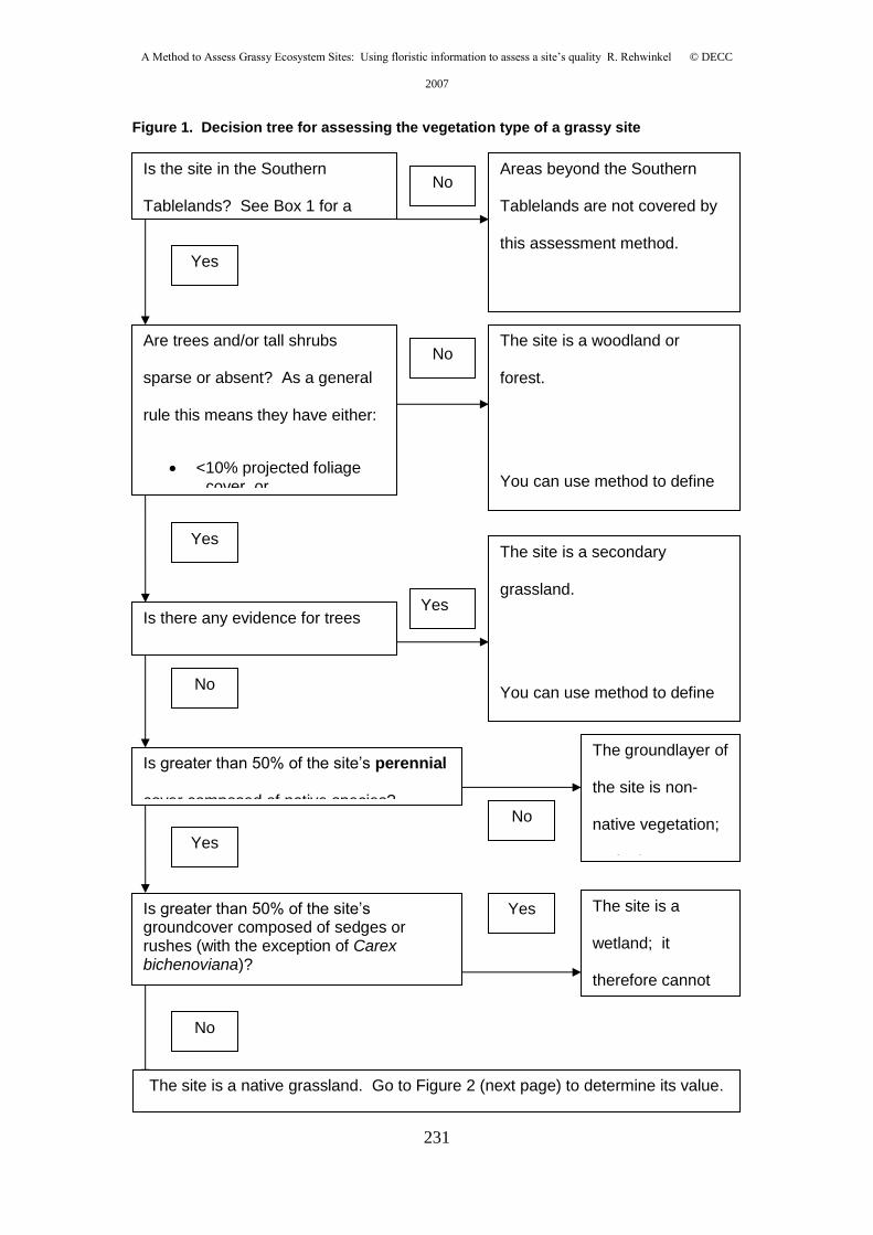
A Method to Assess Grassy Ecosystem Sites: Using floristic information to assess a site’s quality R. Rehwinkel © DECC
2007
231
Figure 1. Decision tree for assessing the vegetation type of a grassy site
Is the site in the Southern
Tablelands? See Box 1 for a
Areas beyond the Southern
Tablelands are not covered by
this assessment method.
No
Yes
Are trees and/or tall shrubs
sparse or absent? As a general
rule this means they have either:
<10% projected foliage cover, or
Yes
No The site is a woodland or
forest.
You can use method to define
Yes
Is there any evidence for trees
formerly on the site? See Box 2.
The site is a secondary
grassland.
You can use method to define No
Is greater than 50% of the site’s perennial
cover composed of native species? No
The groundlayer of
the site is non-
native vegetation;
no further Yes
Is greater than 50% of the site’s groundcover composed of sedges or rushes (with the exception of Carex bichenoviana)?
Yes The site is a
wetland; it
therefore cannot
No
The site is a native grassland. Go to Figure 2 (next page) to determine its value.
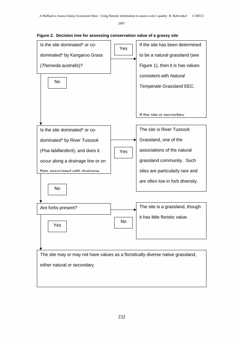
A Method to Assess Grassy Ecosystem Sites: Using floristic information to assess a site’s quality R. Rehwinkel © DECC
2007
232
Figure 2. Decision tree for assessing conservation value of a grassy site
Is the site dominated* or co-
dominated* by Kangaroo Grass
(Themeda australis)?
If the site has been determined
to be a natural grassland (see
Figure 1), then it is has values
consistent with Natural
Temperate Grassland EEC.
If the site is secondary
Yes
No
Yes
Is the site dominated* or co-
dominated* by River Tussock
(Poa labillardierii), and does it
occur along a drainage line or on
flats associated with drainage
The site is River Tussock
Grassland, one of the
associations of the natural
grassland community. Such
sites are particularly rare and
are often low in forb diversity.
Such sites have value No
No
The site is a grassland, though
it has little floristic value.
Yes
The site may or may not have values as a floristically diverse native grassland,
either natural or secondary.
Are forbs present?
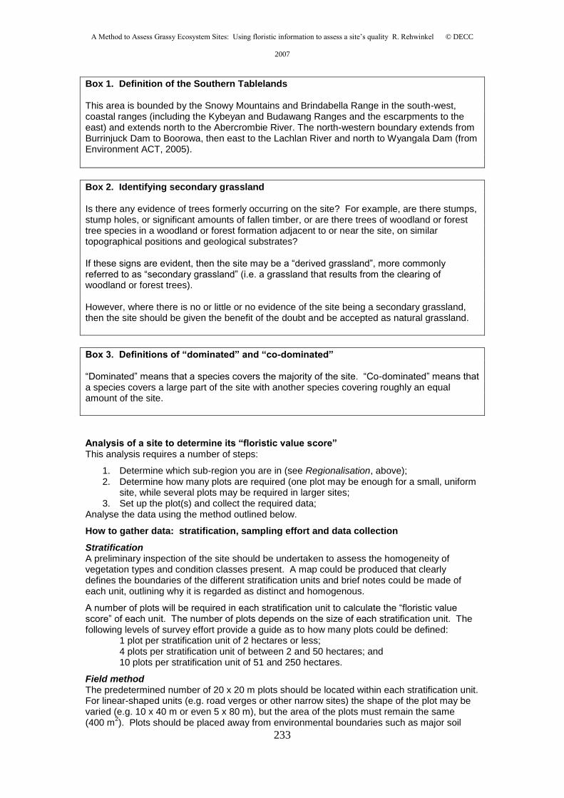
A Method to Assess Grassy Ecosystem Sites: Using floristic information to assess a site’s quality R. Rehwinkel © DECC
2007
233
Box 1. Definition of the Southern Tablelands This area is bounded by the Snowy Mountains and Brindabella Range in the south-west, coastal ranges (including the Kybeyan and Budawang Ranges and the escarpments to the east) and extends north to the Abercrombie River. The north-western boundary extends from Burrinjuck Dam to Boorowa, then east to the Lachlan River and north to Wyangala Dam (from Environment ACT, 2005).
Box 2. Identifying secondary grassland Is there any evidence of trees formerly occurring on the site? For example, are there stumps, stump holes, or significant amounts of fallen timber, or are there trees of woodland or forest tree species in a woodland or forest formation adjacent to or near the site, on similar topographical positions and geological substrates? If these signs are evident, then the site may be a “derived grassland”, more commonly referred to as “secondary grassland” (i.e. a grassland that results from the clearing of woodland or forest trees). However, where there is no or little or no evidence of the site being a secondary grassland, then the site should be given the benefit of the doubt and be accepted as natural grassland.
Box 3. Definitions of “dominated” and “co-dominated” “Dominated” means that a species covers the majority of the site. “Co-dominated” means that a species covers a large part of the site with another species covering roughly an equal amount of the site.
Analysis of a site to determine its “floristic value score” This analysis requires a number of steps:
1. Determine which sub-region you are in (see Regionalisation, above); 2. Determine how many plots are required (one plot may be enough for a small, uniform
site, while several plots may be required in larger sites; 3. Set up the plot(s) and collect the required data;
Analyse the data using the method outlined below.
How to gather data: stratification, sampling effort and data collection
Stratification A preliminary inspection of the site should be undertaken to assess the homogeneity of vegetation types and condition classes present. A map could be produced that clearly defines the boundaries of the different stratification units and brief notes could be made of each unit, outlining why it is regarded as distinct and homogenous.
A number of plots will be required in each stratification unit to calculate the “floristic value score” of each unit. The number of plots depends on the size of each stratification unit. The following levels of survey effort provide a guide as to how many plots could be defined:
1 plot per stratification unit of 2 hectares or less; 4 plots per stratification unit of between 2 and 50 hectares; and 10 plots per stratification unit of 51 and 250 hectares.
Field method The predetermined number of 20 x 20 m plots should be located within each stratification unit. For linear-shaped units (e.g. road verges or other narrow sites) the shape of the plot may be varied (e.g. 10 x 40 m or even 5 x 80 m), but the area of the plots must remain the same (400 m
2). Plots should be placed away from environmental boundaries such as major soil
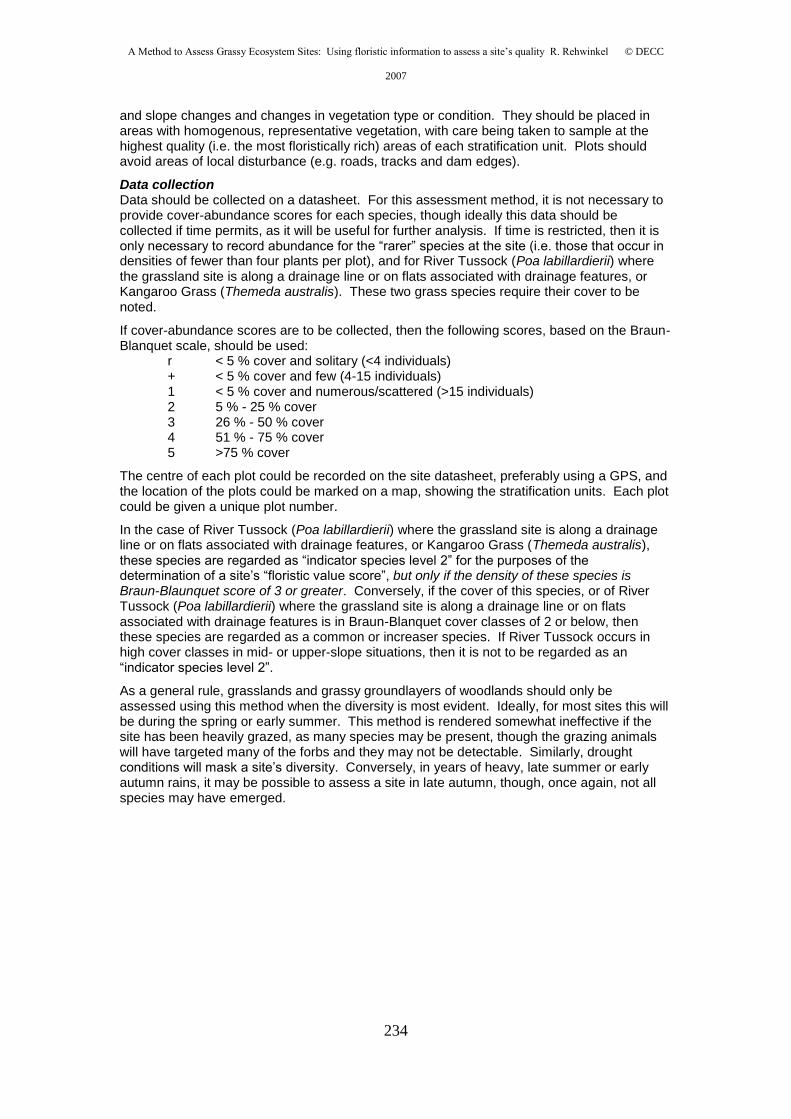
A Method to Assess Grassy Ecosystem Sites: Using floristic information to assess a site’s quality R. Rehwinkel © DECC
2007
234
and slope changes and changes in vegetation type or condition. They should be placed in areas with homogenous, representative vegetation, with care being taken to sample at the highest quality (i.e. the most floristically rich) areas of each stratification unit. Plots should avoid areas of local disturbance (e.g. roads, tracks and dam edges).
Data collection Data should be collected on a datasheet. For this assessment method, it is not necessary to provide cover-abundance scores for each species, though ideally this data should be collected if time permits, as it will be useful for further analysis. If time is restricted, then it is only necessary to record abundance for the “rarer” species at the site (i.e. those that occur in densities of fewer than four plants per plot), and for River Tussock (Poa labillardierii) where the grassland site is along a drainage line or on flats associated with drainage features, or Kangaroo Grass (Themeda australis). These two grass species require their cover to be noted.
If cover-abundance scores are to be collected, then the following scores, based on the Braun-Blanquet scale, should be used:
r < 5 % cover and solitary (<4 individuals) + < 5 % cover and few (4-15 individuals) 1 < 5 % cover and numerous/scattered (>15 individuals) 2 5 % - 25 % cover 3 26 % - 50 % cover 4 51 % - 75 % cover 5 >75 % cover
The centre of each plot could be recorded on the site datasheet, preferably using a GPS, and the location of the plots could be marked on a map, showing the stratification units. Each plot could be given a unique plot number.
In the case of River Tussock (Poa labillardierii) where the grassland site is along a drainage line or on flats associated with drainage features, or Kangaroo Grass (Themeda australis), these species are regarded as “indicator species level 2” for the purposes of the determination of a site’s “floristic value score”, but only if the density of these species is Braun-Blaunquet score of 3 or greater. Conversely, if the cover of this species, or of River Tussock (Poa labillardierii) where the grassland site is along a drainage line or on flats associated with drainage features is in Braun-Blanquet cover classes of 2 or below, then these species are regarded as a common or increaser species. If River Tussock occurs in high cover classes in mid- or upper-slope situations, then it is not to be regarded as an “indicator species level 2”.
As a general rule, grasslands and grassy groundlayers of woodlands should only be assessed using this method when the diversity is most evident. Ideally, for most sites this will be during the spring or early summer. This method is rendered somewhat ineffective if the site has been heavily grazed, as many species may be present, though the grazing animals will have targeted many of the forbs and they may not be detectable. Similarly, drought conditions will mask a site’s diversity. Conversely, in years of heavy, late summer or early autumn rains, it may be possible to assess a site in late autumn, though, once again, not all species may have emerged.
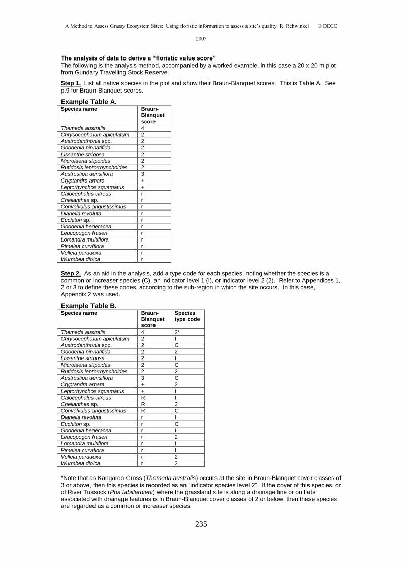
A Method to Assess Grassy Ecosystem Sites: Using floristic information to assess a site’s quality R. Rehwinkel © DECC
2007
235
The analysis of data to derive a “floristic value score”
The following is the analysis method, accompanied by a worked example, in this case a 20 x 20 m plot from Gundary Travelling Stock Reserve.
Step 1. List all native species in the plot and show their Braun-Blanquet scores. This is Table A. See
p.9 for Braun-Blanquet scores.
Example Table A. Species name Braun-
Blanquet score
Themeda australis 4
Chrysocephalum apiculatum 2
Austrodanthonia spp. 2
Goodenia pinnatifida 2
Lissanthe strigosa 2
Microlaena stipoides 2
Rutidosis leptorrhynchoides 2
Austrostipa densiflora 3
Cryptandra amara +
Leptorhynchos squamatus +
Calocephalus citreus r
Cheilanthes sp. r
Convolvulus angustissimus r
Dianella revoluta r
Euchiton sp. r
Goodenia hederacea r
Leucopogon fraseri r
Lomandra multiflora r
Pimelea curviflora r
Velleia paradoxa r
Wurmbea dioica r
Step 2. As an aid in the analysis, add a type code for each species, noting whether the species is a
common or increaser species (C), an indicator level 1 (I), or indicator level 2 (2). Refer to Appendices 1, 2 or 3 to define these codes, according to the sub-region in which the site occurs. In this case, Appendix 2 was used.
Example Table B. Species name Braun-
Blanquet score
Species type code
Themeda australis 4 2*
Chrysocephalum apiculatum 2 I
Austrodanthonia spp. 2 C
Goodenia pinnatifida 2 2
Lissanthe strigosa 2 I
Microlaena stipoides 2 C
Rutidosis leptorrhynchoides 2 2
Austrostipa densiflora 3 C
Cryptandra amara + 2
Leptorhynchos squamatus + I
Calocephalus citreus R I
Cheilanthes sp. R 2
Convolvulus angustissimus R C
Dianella revoluta r I
Euchiton sp. r C
Goodenia hederacea r I
Leucopogon fraseri r 2
Lomandra multiflora r I
Pimelea curviflora r I
Velleia paradoxa r 2
Wurmbea dioica r 2
*Note that as Kangaroo Grass (Themeda australis) occurs at the site in Braun-Blanquet cover classes of 3 or above, then this species is recorded as an “indicator species level 2”. If the cover of this species, or of River Tussock (Poa labillardierii) where the grassland site is along a drainage line or on flats associated with drainage features is in Braun-Blanquet cover classes of 2 or below, then these species are regarded as a common or increaser species.
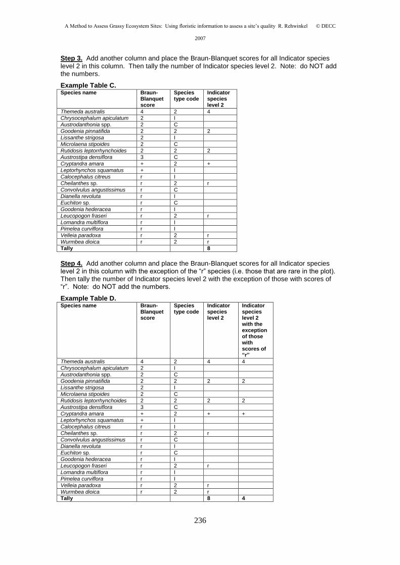
A Method to Assess Grassy Ecosystem Sites: Using floristic information to assess a site’s quality R. Rehwinkel © DECC
2007
236
Step 3. Add another column and place the Braun-Blanquet scores for all Indicator species level 2 in this column. Then tally the number of Indicator species level 2. Note: do NOT add the numbers.
Example Table C. Species name Braun-
Blanquet score
Species type code
Indicator species level 2
Themeda australis 4 2 4
Chrysocephalum apiculatum 2 I
Austrodanthonia spp. 2 C
Goodenia pinnatifida 2 2 2
Lissanthe strigosa 2 I
Microlaena stipoides 2 C
Rutidosis leptorrhynchoides 2 2 2
Austrostipa densiflora 3 C
Cryptandra amara + 2 +
Leptorhynchos squamatus + I
Calocephalus citreus r I
Cheilanthes sp. r 2 r
Convolvulus angustissimus r C
Dianella revoluta r I
Euchiton sp. r C
Goodenia hederacea r I
Leucopogon fraseri r 2 r
Lomandra multiflora r I
Pimelea curviflora r I
Velleia paradoxa r 2 r
Wurmbea dioica r 2 r
Tally 8
Step 4. Add another column and place the Braun-Blanquet scores for all Indicator species level 2 in this column with the exception of the “r” species (i.e. those that are rare in the plot). Then tally the number of Indicator species level 2 with the exception of those with scores of “r”. Note: do NOT add the numbers.
Example Table D. Species name Braun-
Blanquet score
Species type code
Indicator species level 2
Indicator species level 2 with the exception of those with scores of “r”
Themeda australis 4 2 4 4
Chrysocephalum apiculatum 2 I
Austrodanthonia spp. 2 C
Goodenia pinnatifida 2 2 2 2
Lissanthe strigosa 2 I
Microlaena stipoides 2 C
Rutidosis leptorrhynchoides 2 2 2 2
Austrostipa densiflora 3 C
Cryptandra amara + 2 + +
Leptorhynchos squamatus + I
Calocephalus citreus r I
Cheilanthes sp. r 2 r
Convolvulus angustissimus r C
Dianella revoluta r I
Euchiton sp. r C
Goodenia hederacea r I
Leucopogon fraseri r 2 r
Lomandra multiflora r I
Pimelea curviflora r I
Velleia paradoxa r 2 r
Wurmbea dioica r 2 r
Tally 8 4
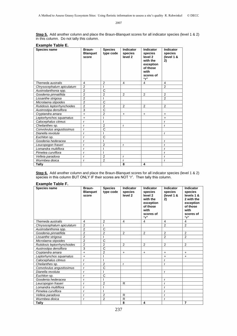
A Method to Assess Grassy Ecosystem Sites: Using floristic information to assess a site’s quality R. Rehwinkel © DECC
2007
237
Step 5. Add another column and place the Braun-Blanquet scores for all indicator species (level 1 & 2)
in this column. Do not tally this column.
Example Table E. Species name Braun-
Blanquet score
Species type code
Indicator species level 2
Indicator species level 2 with the exception of those with scores of “r”
Indicator species (level 1 & 2)
Themeda australis 4 2 4 4 4
Chrysocephalum apiculatum 2 I 2
Austrodanthonia spp. 2 C
Goodenia pinnatifida 2 2 2 2 2
Lissanthe strigosa 2 I 2
Microlaena stipoides 2 C
Rutidosis leptorrhynchoides 2 2 2 2 2
Austrostipa densiflora 3 C
Cryptandra amara + 2 + + +
Leptorhynchos squamatus + I +
Calocephalus citreus r I r
Cheilanthes sp. r 2 r r
Convolvulus angustissimus r C
Dianella revolute r I r
Euchiton sp. r C
Goodenia hederacea r I r
Leucopogon fraseri r 2 r r
Lomandra multiflora r I r
Pimelea curviflora r I r
Velleia paradoxa r 2 r r
Wurmbea dioica r 2 r r
Tally 8 4
Step 6. Add another column and place the Braun-Blanquet scores for all indicator species (level 1 & 2)
species in this column BUT ONLY IF their scores are NOT “r”. Then tally this column.
Example Table F. Species name Braun-
Blanquet score
Species type code
Indicator species level 2
Indicator species level 2 with the exception of those with scores of “r”
Indicator species (level 1 & 2)
Indicator species levels 1 & 2 with the exception of those with scores of “r”
Themeda australis 4 2 4 4 4 4
Chrysocephalum apiculatum 2 I 2 2
Austrodanthonia spp. 2 C
Goodenia pinnatifida 2 2 2 2 2 2
Lissanthe strigosa 2 I 2 2
Microlaena stipoides 2 C
Rutidosis leptorrhynchoides 2 2 2 2 2 2
Austrostipa densiflora 3 C
Cryptandra amara + 2 + + + +
Leptorhynchos squamatus + I + +
Calocephalus citreus r I r
Cheilanthes sp. r 2 r r
Convolvulus angustissimus r C
Dianella revoluta r I r
Euchiton sp. r C
Goodenia hederacea r I r
Leucopogon fraseri r 2 R r
Lomandra multiflora r I r
Pimelea curviflora r I r
Velleia paradoxa r 2 R r
Wurmbea dioica r 2 R r
Tally 8 4 7
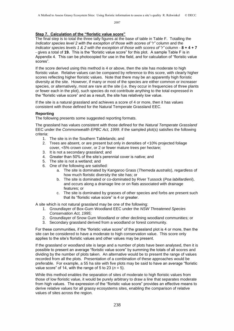
A Method to Assess Grassy Ecosystem Sites: Using floristic information to assess a site’s quality R. Rehwinkel © DECC
2007
238
Step 7. Calculation of the “floristic value score” The final step is to total the three tally figures at the base of table in Table F. Totalling the Indicator species level 2 with the exception of those with scores of “r” column and the Indicator species levels 1 & 2 with the exception of those with scores of “r” column - 8 + 4 + 7 - gives a total of 19. This is the “floristic value score” for this plot. A sample Table F is in Appendix 4. This can be photocopied for use in the field, and for calculation of “floristic value scores”.
If the score derived using this method is 4 or above, then the site has moderate to high floristic value. Relative values can be compared by reference to this score, with clearly higher scores reflecting higher floristic values. Note that there may be an apparently high floristic diversity at the site. However, if many or most of the species are either common or increaser species, or alternatively, most are rare at the site (i.e. they occur in frequencies of three plants or fewer each in the plot), such species do not contribute anything to the total expressed in the “floristic value score” and as a result, the site has relatively low value.
If the site is a natural grassland and achieves a score of 4 or more, then it has values consistent with those defined for the Natural Temperate Grassland EEC.
Reporting The following presents some suggested reporting formats.
The grassland has values consistent with those defined for the Natural Temperate Grassland EEC under the Commonwealth EPBC Act, 1999. if the sampled plot(s) satisfies the following criteria:
1. The site is in the Southern Tablelands; and 2. Trees are absent, or are present but only in densities of <10% projected foliage
cover, <5% crown cover, or 2 or fewer mature trees per hectare; 3. It is not a secondary grassland; and 4. Greater than 50% of the site’s perennial cover is native; and 5. The site is not a wetland; and 6. One of the following are satisfied:
a. The site is dominated by Kangaroo Grass (Themeda australis), regardless of how much floristic diversity the site has; or
b. The site is dominated or co-dominated by River Tussock (Poa labillardierii), and occurs along a drainage line or on flats associated with drainage features; or
c. The site is dominated by grasses of other species and forbs are present such that its “floristic value score” is 4 or greater.
A site which is not natural grassland may be one of the following: 1. Groundlayer of Box-Gum Woodland EEC under the NSW Threatened Species
Conservation Act, 1995; 2. Groundlayer of Snow Gum Woodland or other declining woodland communities; or 3. Secondary grassland derived from a woodland or forest community.
For these communities, if the “floristic value score” of the grassland plot is 4 or more, then the site can be considered to have a moderate to high conservation value. This score only applies to the site’s floristic values and other values may be present.
If the grassland or woodland site is large and a number of plots have been analysed, then it is possible to present an average “floristic value score” by summing the totals of all scores and dividing by the number of plots taken. An alternative would be to present the range of values recorded from all the plots. Presentation of a combination of these approaches would be preferable. For example, a 55 ha site with five plots may be said to have an average “floristic value score” of 14, with the range of 5 to 23 (n = 5).
While this method enables the separation of sites of moderate to high floristic values from those of low floristic value, it would be purely arbitrary to draw a line that separates moderate from high values. The expression of the “floristic value score” provides an effective means to derive relative values for all grassy ecosystems sites, enabling the comparison of relative values of sites across the region.
A Method to Assess Grassy Ecosystem Sites: Using floristic information to assess a site’s quality R. Rehwinkel © DECC
2007
239
Acknowledgments and disclaimer This methodology has been developed with the inputs of data and ideas of many people. I thank Sarah Sharp, David Eddy and Greg Baines variously for major impetus, inputs into the development of this concept, application of the idea, refinement and review of the “increaser species”, discussions about the “cut-off lines”, suggestions for text and flow-charts, analysis of data, and review of previous versions of this document. John Briggs is also thanked for his support and technical inputs. I thank Sally Stephens and the ANPC for providing the impetus and opportunity to present this information and Margaret Ning who assisted me in the training course which introduced this method. Margaret provided very useful suggestions to make the document easier to use.
I thank the following people for the data which has enabled the “significance scores” to be applied to each of the grassy ecosystem species: Sarah Sharp, Isobel Crawford, Alison Rowell, John Benson, David Eddy and Greg Baines.
The ideas and concepts presented in this document are those of the author and not the opinions of the Director-General of the NSW Department of Environment and Climate Change.
References
ACT Government (2004) Woodlands for Wildlife: ACT Lowland Woodland Conservation Strategy. Action Plan No. 27 (Environment ACT, Canberra).
ACT Government (2005) A Vision Splendid of the Grassy Plains Extended: ACT Lowland Native Grassland Conservation Strategy. Action Plan No. 28 (Arts, Heritage and Environment, Canberra).
Environment ACT (2005) National Recovery Plan for Natural Temperate Grassland of the Southern Tablelands (NSW and ACT): an endangered ecological community (Environment ACT, Canberra).
Langford, C.M., Simpson, P.C., Garden, D.L., Eddy, D.A., Keys, M.J., Rehwinkel, R., & Johnston, W.H. (2004) Managing Native Pastures For Agriculture and Conservation NSW Department of Primary Industries.
Lunt, I. (1995) European Management of Remnant Grassy Forests and Woodlands in South-eastern Australia – Past, Present and Future? Victorian Naturalist Vol 112(6) p. 239-249
McIntyre, S., McIvor, J.C. & Heard, K.M. (editors) (2002) Managing & Conserving Grassy Woodlands CSIRO Publishing
Prober, S & Thiele, K (1993) The Ecology and Genetics of Remnant Grassy White Box Woodlands in relation to their Conservation. Victorian Naturalist Vol 110(1) p. 30-36
Tindall, D., Pennay, C., Tozer, M., Turner, K. & Keith, D. (2006) Native vegetation map report series. No.4 NSW Department of Environment and Conservation, NSW Department of Infrastructure, Planning & Natural Resources.
Thomas, V., Gellie, N. & Harrison, T. (200) Forest Ecosystem Classification and Mapping for the Southern CRA Region. NSW National Parks and Wildlife Service Southern Directorate. A report undertaken for the NSW CRA/RFA Steering Committee. Project Number NS 08EH
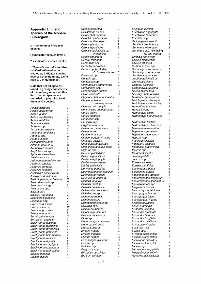
A Method to Assess Grassy Ecosystem Sites: Using floristic information to assess a site’s quality R. Rehwinkel © DECC
2007
240
Appendix 1. List of species of the Monaro Sub-region.
C = common or increaser species; I = indicator species level 1; 2 = indicator species level 2; * Themeda australis and Poa labillardierii need to be treated as indicator species level 2 if they dominate a site (see p. 9 in guidelines). Note that not all species found in grassy ecosystems of the sub-region are on this list. If other species are recorded in your plot, treat them as C species. Acacia dawsonii 2 Acacia doratoxylon 2 Acacia gunnii 2 Acacia siculiformis 2 Acacia ulicifolia 2 Acacia uncinata 2 Acaena spp. C Acrotriche serrulata 2 Adiantum aethiopica 2 Agrostis spp. C Ajuga australis I Allocasuarina nana 2 Alternanthera sp.A C Ammobium alatum 2 Amphibromus spp. C Aphanes australiana C Aristida ramosa C Arthropodium milleflorum 2 Asperula ambleia 2 Asperula conferta I Asperula scoparia I Asplenium flabellifolium 2 Astroloma humifusum 2 Australopyrum pectinatum C Austrodanthonia spp. C Austrofestuca spp. 2 Austrostipa spp. C Baekia utilis C Banksia marginata 2 Billardiera scandens 2 Blechnum spp. 2 Bossiaea buxifolia 2 Bossiaea foliosa C Bossiaea prostrata 2 Bossiaea riparia 2 Bothriochloa macra C Botrichium australe 2 Brachycome aculeata 2 Brachycome decipiens 2 Brachycome diversifolia 2 Brachycome graminea 2 Brachycome heterodonta I Brachycome radicans 2 Brachycome rigidula 2 Brachycome scapigera 2 Brachycome spathulata 2 Brachyloma daphnoides 2 Bulbine bulbosa 2 Bulbine glauca 2
Caesia calliantha 2 Callistemon sieberi 2 Calocephalus citreus 2 Calochilus robertsonii 2 Calotis anthemoides 2 Calotis glandulosa 2 Calotis lappulacea 2 Calotis scabiosifolia var.
integrifolia 2 Calotis scapigera 2 Calytrix tetragona 2 Cardamine spp. 2 Carex bichenoviana 2 Carex spp. (excluding
C. bichenoviana) C Cassinia spp. C Centella spp. 2 Centipeda spp. C Chamaesyce drummondii C Cheilanthes spp. 2 Chenopodium pumilio C Chloris truncata C Chrysocephalum apiculatum I Chrysocephalum
semipapposum I Clematis microphylla 2 Convolvulus angustissimus C Cotula alpina 2 Cotula australis C Craspedia spp. 2 Crassula spp. C Cryptandra amara 2 Cullen microcephalum 2 Cullen tenax 2 Cymbonotus spp. C Cymbonpogon refractus 2 Cynodon dactylis C Cynoglossum australe 2 Cynoglossum suaveolens C Cyperus spp. C Daucus glochidiatus C Daviesia genistifolia 2 Daviesia leptophylla 2 Daviesia mimosoides 2 Daviesia ulicifolia C Derwentia perfoliata 2 Desmodium brachypodium 2 Desmodium varians 2 Deyeuxia quadriseta 2 Dianella longifolia 2 Dianella revoluta 2 Dianella tasmanica 2 Dichanthium sericeum 2 Dichelachne spp. C Dichondra repens C Dichondra sp.A C Dichopogon fimbriatus 2 Dillwynia spp. 2 Diplarrena moraea 2 Dipodium punctatum 2 Discaria pubescens 2 Diuris spp. 2 Dodonaea procumbens 2 Dodonaea viscose 2 Drosera peltata C Einadia nutans C Einadia trigonos 2 Elymus scaber C Enneapogon nigricans C Epacris spp. 2 Epilolium spp. C Eragrostis spp. C Eriochilus cucullatus 2 Erodium crinitum C
Eryngium ovinum 2 Eucalyptus aggregata 2 Eucalyptus lacrimans 2 Euchiton spp. C Galium gaudichaudii 2 Gentiana bredboensis 2 Geranium antrorsum 2 Geranium spp. (excluding
G. antrorsum) C Gingidia harveyana 2 Glycine clandestina 2 Glycine tabacina I Gompholobium spp. 2 Gonocarpus micranthus 2 Gonocarpus tetragynus 2 Goodenia hederacea 2 Goodenia pinnatifida 2 Grevillea lanigera 2 Gynatrix pulchella 2 Gypsophylla tubulosa C Hakea microcarpa 2 Haloragis heterophylla I Hardenbergia violacea 2 Helichrysum rutidolepis 2 Helichrysum scorpioides 2 Hemarthria uncinata 2 Hovea linearis 2 Hydrocotyle algida C Hydrocotyle peduncularis
C Hydrocotyle laxiflora I Hydrocotyle peduncularis C Hymenanthera dentata C Hypericum gramineum 2 Hypericum japonicum 2 Hypoxis spp. 2 Imperata cylindica C Indigofera australis 2 Isoetopsis graminifolia 2 Isolepis spp. C Isotoma fluviatilis 2 Joycea pallida C Juncus spp. C Kunzea ericoides C Kunzea parvifolia C Lagenifera stipitata 2 Laxmannia gracilis 2 Lepidosperma laterale 2 Leptorhynchos elongatus 2 Leptorhynchos squamatus I Leptospermum spp. C Lespedeza juncea 2 Leucochrysum albicans 2 Leucopogon fletcheri 2 Leucopogon fraseri 2 Leucopogon virgatus 2 Liliopsis polyantha 2 Linum marginale 2 Lissanthe strigosa 2 Lomandra bracteata 2 Lomandra filiformis 2 Lomandra longifolia 2 Lomandra multiflora 2 Lomatia myricoides 2 Lotus australis 2 Luzula spp. 2 Lythrum hyssopifolia C Melichrus urceolatus 2 Microlaena stipoides C Microseris lanceolata 2 Microtis spp. 2 Mitrasacme serpylifolia 2 Muelenbeckia axilaris 2 Neopaxia australasica 2
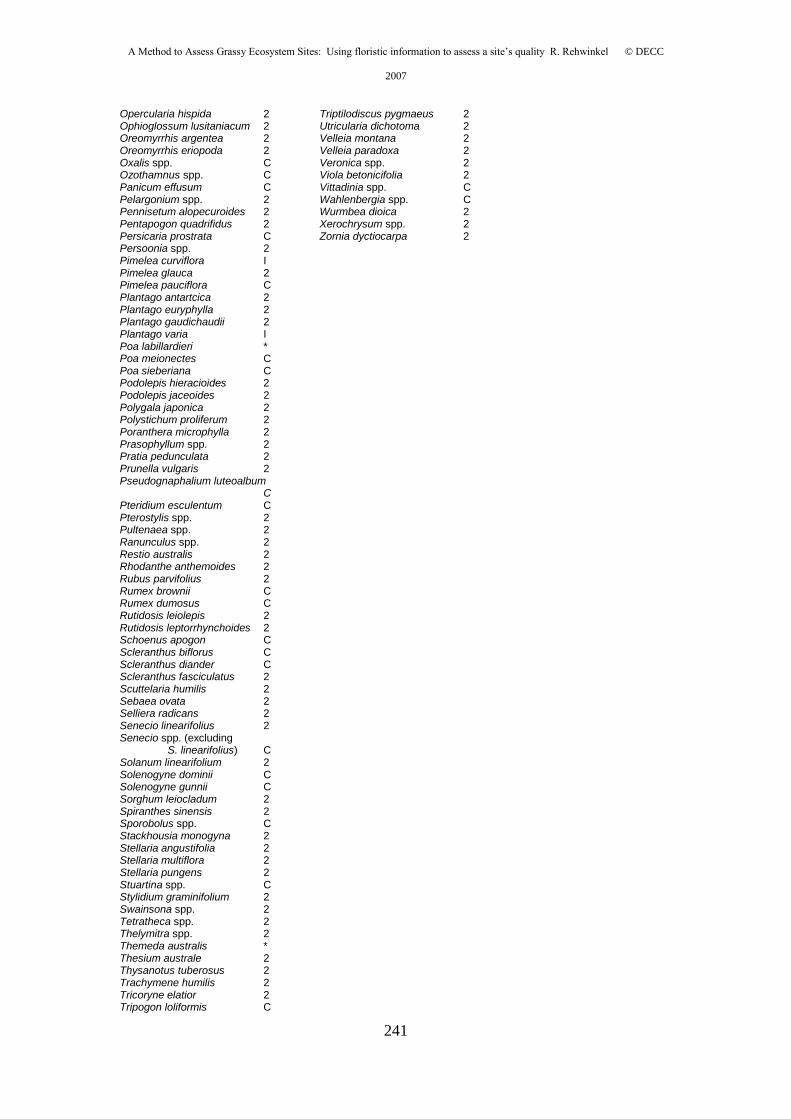
A Method to Assess Grassy Ecosystem Sites: Using floristic information to assess a site’s quality R. Rehwinkel © DECC
2007
241
Opercularia hispida 2 Ophioglossum lusitaniacum 2 Oreomyrrhis argentea 2 Oreomyrrhis eriopoda 2 Oxalis spp. C Ozothamnus spp. C Panicum effusum C Pelargonium spp. 2 Pennisetum alopecuroides 2 Pentapogon quadrifidus 2 Persicaria prostrata C Persoonia spp. 2 Pimelea curviflora I Pimelea glauca 2 Pimelea pauciflora C Plantago antartcica 2 Plantago euryphylla 2 Plantago gaudichaudii 2 Plantago varia I Poa labillardieri * Poa meionectes C Poa sieberiana C Podolepis hieracioides 2 Podolepis jaceoides 2 Polygala japonica 2 Polystichum proliferum 2 Poranthera microphylla 2 Prasophyllum spp. 2 Pratia pedunculata 2 Prunella vulgaris 2 Pseudognaphalium luteoalbum
C Pteridium esculentum C Pterostylis spp. 2 Pultenaea spp. 2 Ranunculus spp. 2 Restio australis 2 Rhodanthe anthemoides 2 Rubus parvifolius 2 Rumex brownii C Rumex dumosus C Rutidosis leiolepis 2 Rutidosis leptorrhynchoides 2 Schoenus apogon C Scleranthus biflorus C Scleranthus diander C Scleranthus fasciculatus 2 Scuttelaria humilis 2 Sebaea ovata 2 Selliera radicans 2 Senecio linearifolius 2 Senecio spp. (excluding
S. linearifolius) C Solanum linearifolium 2 Solenogyne dominii C Solenogyne gunnii C Sorghum leiocladum 2 Spiranthes sinensis 2 Sporobolus spp. C Stackhousia monogyna 2 Stellaria angustifolia 2 Stellaria multiflora 2 Stellaria pungens 2 Stuartina spp. C Stylidium graminifolium 2 Swainsona spp. 2 Tetratheca spp. 2 Thelymitra spp. 2 Themeda australis * Thesium australe 2 Thysanotus tuberosus 2 Trachymene humilis 2 Tricoryne elatior 2 Tripogon loliformis C
Triptilodiscus pygmaeus 2 Utricularia dichotoma 2 Velleia montana 2 Velleia paradoxa 2 Veronica spp. 2 Viola betonicifolia 2 Vittadinia spp. C Wahlenbergia spp. C Wurmbea dioica 2 Xerochrysum spp. 2 Zornia dyctiocarpa 2
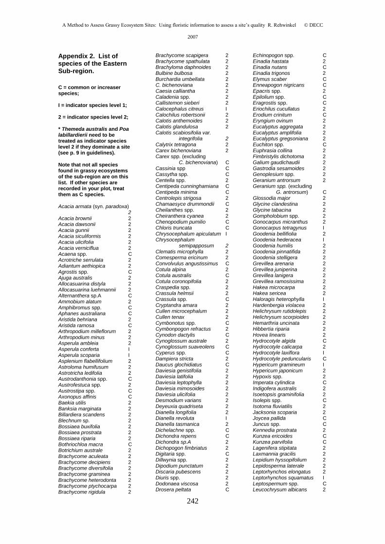
A Method to Assess Grassy Ecosystem Sites: Using floristic information to assess a site’s quality R. Rehwinkel © DECC
2007
242
Appendix 2. List of species of the Eastern Sub-region.
C = common or increaser species; I = indicator species level 1; 2 = indicator species level 2; * Themeda australis and Poa labillardierii need to be treated as indicator species level 2 if they dominate a site (see p. 9 in guidelines). Note that not all species found in grassy ecosystems of the sub-region are on this list. If other species are recorded in your plot, treat them as C species. Acacia armata (syn. paradoxa)
2 Acacia brownii 2 Acacia dawsonii 2 Acacia gunnii 2 Acacia siculiformis 2 Acacia ulicifolia 2 Acacia verniciflua 2 Acaena spp. C Acrotriche serrulata 2 Adiantum aethiopica 2 Agrostis spp. C Ajuga australis 2 Allocasuarina distyla 2 Allocasuarina luehmannii 2 Alternanthera sp.A C Ammobium alatum 2 Amphibromus spp. C Aphanes australiana C Aristida behriana 2 Aristida ramosa C Arthropodium milleflorum 2 Arthropodium minus 2 Asperula ambleia 2 Asperula conferta I Asperula scoparia I Asplenium flabellifolium 2 Astroloma humifusum 2 Astrotricha ledifolia 2 Austrodanthonia spp. C Austrofestuca spp. 2 Austrostipa spp. C Axonopus affinis C Baekia utilis 2 Banksia marginata 2 Billardiera scandens 2 Blechnum sp. 2 Bossiaea buxifolia 2 Bossiaea prostrata 2 Bossiaea riparia 2 Bothriochloa macra C Botrichium australe 2 Brachycome aculeata 2 Brachycome decipiens 2 Brachycome diversifolia 2 Brachycome graminea 2 Brachycome heterodonta 2 Brachycome ptychocarpa 2 Brachycome rigidula 2
Brachycome scapigera 2 Brachycome spathulata 2 Brachyloma daphnoides 2 Bulbine bulbosa 2 Burchardia umbellata 2 C. bichenoviana 2 Caesia calliantha 2 Caladenia spp. 2 Callistemon sieberi 2 Calocephalus citreus I Calochilus robertsonii 2 Calotis anthemoides 2 Calotis glandulosa 2 Calotis scabiosifolia var.
integrifolia 2 Calytrix tetragona 2 Carex bichenoviana 2 Carex spp. (excluding
C. bichenoviana) C Cassinia spp C Cassytha spp. C Centella spp. 2 Centipeda cunninghamiana C Centipeda minima C Centrolepis strigosa 2 Chamaesyce drummondii C Cheilanthes spp. 2 Cheiranthera cyanea 2 Chenopodium pumilio C Chloris truncata C Chrysocephalum apiculatum I Chrysocephalum
semipapposum 2 Clematis microphylla 2 Comesperma ericinum 2 Convolvulus angustissimus C Cotula alpina 2 Cotula australis C Cotula coronopifolia 2 Craspedia spp. 2 Crassula helmsii 2 Crassula spp. C Cryptandra amara 2 Cullen microcephalum 2 Cullen tenax 2 Cymbonotus spp. C Cymbonpogon refractus 2 Cynodon dactylis C Cynoglossum australe 2 Cynoglossum suaveolens C Cyperus spp. C Dampiera stricta 2 Daucus glochidiatus C Daviesia genistifolia 2 Daviesia latifolia 2 Daviesia leptophylla 2 Daviesia mimosoides 2 Daviesia ulicifolia 2 Desmodium varians 2 Deyeuxia quadriseta 2 Dianella longifolia 2 Dianella revoluta I Dianella tasmanica 2 Dichelachne spp. C Dichondra repens C Dichondra sp.A 2 Dichopogon fimbriatus 2 Digitaria spp. C Dillwynia spp. 2 Dipodium punctatum 2 Discaria pubescens 2 Diuris spp. 2 Dodonaea viscosa 2 Drosera peltata C
Echinopogon spp. C Einadia hastata 2 Einadia nutans C Einadia trigonos 2 Elymus scaber C Enneapogon nigricans C Epacris spp. 2 Epilolium spp. C Eragrostis spp. C Eriochilus cucullatus 2 Erodium crinitum C Eryngium ovinum 2 Eucalyptus aggregata 2 Eucalyptus amplifolia 2 Eucalyptus gregsoniana 2 Euchiton spp. C Euphrasia collina 2 Fimbristylis dichotoma 2 Galium gaudichaudii 2 Gastrodia sesamoides 2 Genoplesium spp. 2 Geranium antrorsum 2 Geranium spp. (excluding
G. antrorsum) C Glossodia major 2 Glycine clandestina 2 Glycine tabacina 2 Gompholobium spp. 2 Gonocarpus micranthus 2 Gonocarpus tetragynus I Goodenia bellifiolia 2 Goodenia hederacea I Goodenia humilis 2 Goodenia pinnatifida 2 Goodenia stelligera 2 Grevillea arenaria 2 Grevillea juniperina 2 Grevillea lanigera 2 Grevillea ramosissima 2 Hakea microcarpa 2 Hakea sericea 2 Haloragis heterophylla I Hardenbergia violacea 2 Helichrysum rutidolepis 2 Helichrysum scorpioides 2 Hemarthria uncinata 2 Hibbertia riparia 2 Hovea linearis 2 Hydrocotyle algida C Hydrocotyle calicarpa 2 Hydrocotyle laxiflora I Hydrocotyle peduncularis C Hypericum gramineum I Hypericum japonicum 2 Hypoxis spp. 2 Imperata cylindica C Indigofera australis 2 Isoetopsis graminifolia 2 Isolepis spp. C Isotoma fluviatilis 2 Jacksonia scoparia 2 Joycea pallida C Juncus spp. C Kennedia prostrata 2 Kunzea ericoides C Kunzea parvifolia C Lagenifera stipitata 2 Laxmannia gracilis 2 Lepidium hyssopifolium 2 Lepidosperma laterale 2 Leptorhynchos elongatus 2 Leptorhynchos squamatus I Leptospermum spp. C Leucochrysum albicans 2
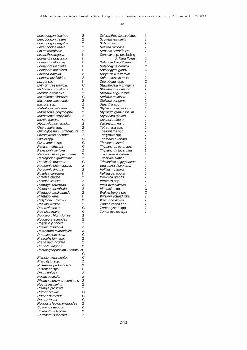
A Method to Assess Grassy Ecosystem Sites: Using floristic information to assess a site’s quality R. Rehwinkel © DECC
2007
243
Leucopogon fletcheri 2 Leucopogon fraseri 2 Leucopogon virgatus 2 Levenhookia dubia 2 Linum marginale 2 Lissanthe strigosa I Lomandra bracteata I Lomandra filiformis I Lomandra longifolia I Lomandra multiflora I Lomatia ilicifolia 2 Lomatia myricoides 2 Luzula spp. I Lythrum hyssopifolia C Melichrus urceolatus I Mentha diemenica 2 Microlaena stipoides C Microseris lanceolata 2 Microtis spp. 2 Mirbelia oxyloboides 2 Mitrasacme polymorpha 2 Mitrasacme serpylifolia 2 Montia fontana C Neopaxia australasica 2 Opercularia spp. 2 Ophioglossum lusitaniacum 2 Oreomyrrhis eriopoda 2 Oxalis spp. C Ozothamnus spp. C Panicum effusum C Patersonia sericea 2 Pennisetum alopecuroides 2 Pentapogon quadrifidus 2 Persicaria prostrata C Persoonia chamaecyce 2 Persoonia linearis 2 Pimelea curviflora I Pimelea glauca 2 Pimelea linifolia 2 Plantago antartcica 2 Plantago euryphylla 2 Plantago gaudichaudii 2 Plantago varia I Platylobium formosa 2 Poa labillardieri * Poa meionectes C Poa sieberiana C Podolepis hieracioides 2 Podolepis jaceoides 2 Polygala japonica 2 Pomax umbellata 2 Poranthera microphylla 2 Portulaca oleracea C Prasophyllum spp. 2 Pratia pedunculata 2 Prunella vulgaris 2 Pseudognaphalium luteoalbum C Pteridium esculentum C Pterostylis spp. 2 Pultenaea pedunculata 2 Pultenaea spp. I Ranunculus spp. 2 Restio australis 2 Rhytidosporum procumbens 2 Rubus parvifolius 2 Rulingia prostrata 2 Rumex brownii C Rumex dumosus C Rumex tenax C Rutidosis leptorhynchoides 2 Schoenus apogon C Scleranthus biflorus 2 Scleranthus diander 2
Scleranthus fasciculatus I Scuttelaria humilis 2 Sebaea ovata 2 Selliera radicans 2 Senecio linearifolius 2 Senecio spp. (excluding
S. linearifolius) C Solanum linearifolium 2 Solenogyne dominii C Solenogyne gunnii C Sorghum leiocladum 2 Spiranthes sinensis 2 Sporobolus spp. C Stackhousia monogyna 2 Stackhousia viminea 2 Stellaria angustifolia 2 Stellaria multiflora 2 Stellaria pungens 2 Stuartina spp. C Stylidium despectum 2 Stylidium graminifolium I Stypandra glauca 2 Styphelia triflora 2 Swiansona recta 2 Tetratheca spp. 2 Thelionema spp. 2 Thelymitra spp. 2 Themeda australis * Thesium australe 2 Thysanotus patersonii 2 Thysanotus tuberosus 2 Trachymene humilis 2 Tricoryne elatior I Triptilodiscus pygmaeus I Utricularia dichotoma 2 Velleia montana 2 Velleia paradoxa 2 Veronica gracilis 2 Veronica spp. 2 Viola betonicifolia 2 Vittadinia spp. C Wahlenbergia spp. C Wilsonia rotundifolia 2 Wurmbea dioica 2 Xanthorrhoea spp. 2 Xerochrysum spp. 2 Zornia dyctiocarpa 2
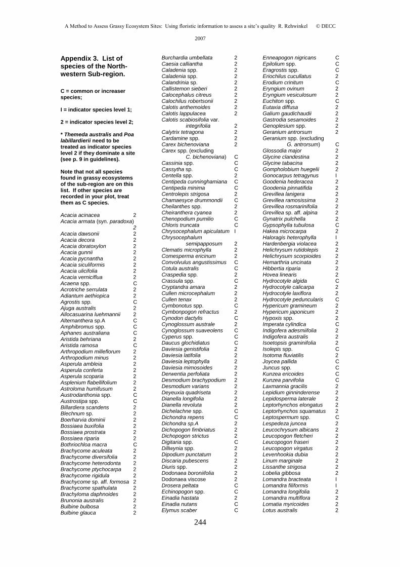
A Method to Assess Grassy Ecosystem Sites: Using floristic information to assess a site’s quality R. Rehwinkel © DECC
2007
244
Appendix 3. List of species of the North-western Sub-region.
C = common or increaser species; I = indicator species level 1; 2 = indicator species level 2; * Themeda australis and Poa labillardierii need to be treated as indicator species level 2 if they dominate a site (see p. 9 in guidelines). Note that not all species found in grassy ecosystems of the sub-region are on this list. If other species are recorded in your plot, treat them as C species. Acacia acinacea 2 Acacia armata (syn. paradoxa)
2 Acacia dawsonii 2 Acacia decora 2 Acacia doratoxylon 2 Acacia gunnii 2 Acacia pycnantha 2 Acacia siculiformis 2 Acacia ulicifolia 2 Acacia verniciflua 2 Acaena spp. C Acrotriche serrulata 2 Adiantum aethiopica 2 Agrostis spp. C Ajuga australis 2 Allocasuarina luehmannii 2 Alternanthera sp.A C Amphibromus spp. C Aphanes australiana C Aristida behriana 2 Aristida ramosa C Arthropodium milleflorum 2 Arthropodium minus 2 Asperula ambleia 2 Asperula conferta 2 Asperula scoparia 2 Asplenium flabellifolium 2 Astroloma humifusum 2 Austrodanthonia spp. C Austrostipa spp. C Billardiera scandens 2 Blechnum sp. 2 Boerharvia dominii 2 Bossiaea buxifolia 2 Bossiaea prostrata 2 Bossiaea riparia 2 Bothriochloa macra C Brachycome aculeata 2 Brachycome diversifolia 2 Brachycome heterodonta 2 Brachycome ptychocarpa 2 Brachycome rigidula 2 Brachycome sp. aff. formosa 2 Brachycome spathulata 2 Brachyloma daphnoides 2 Brunonia australis 2 Bulbine bulbosa 2 Bulbine glauca 2
Burchardia umbellata 2 Caesia calliantha 2 Caladenia spp. 2 Caladenia spp. 2 Calandrinia sp. 2 Callistemon sieberi 2 Calocephalus citreus 2 Calochilus robertsonii 2 Calotis anthemoides 2 Calotis lappulacea 2 Calotis scabiosifolia var.
integrifolia 2 Calytrix tetragona 2 Cardamine spp. 2 Carex bichenoviana 2 Carex spp. (excluding
C. bichenoviana) C Cassinia spp. C Cassytha sp. C Centella spp. 2 Centipeda cunninghamiana C Centipeda minima C Centrolepis strigosa 2 Chamaesyce drummondii C Cheilanthes spp. 2 Cheiranthera cyanea 2 Chenopodium pumilio C Chloris truncata C Chrysocephalum apiculatum I Chrysocephalum
semipapposum 2 Clematis microphylla 2 Comesperma ericinum 2 Convolvulus angustissimus C Cotula australis C Craspedia spp. 2 Crassula spp. C Cryptandra amara 2 Cullen microcephalum 2 Cullen tenax 2 Cymbonotus spp. C Cymbonpogon refractus 2 Cynodon dactylis C Cynoglossum australe 2 Cynoglossum suaveolens C Cyperus spp. C Daucus glochidiatus C Daviesia genistifolia 2 Daviesia latifolia 2 Daviesia leptophylla 2 Daviesia mimosoides 2 Derwentia perfoliata 2 Desmodium brachypodium 2 Desmodium varians 2 Deyeuxia quadriseta 2 Dianella longifolia 2 Dianella revoluta 2 Dichelachne spp. C Dichondra repens C Dichondra sp.A 2 Dichopogon fimbriatus 2 Dichopogon strictus 2 Digitaria spp. C Dillwynia spp. 2 Dipodium punctatum 2 Discaria pubescens 2 Diuris spp. 2 Dodonaea boroniifolia 2 Dodonaea viscose 2 Drosera peltata C Echinopogon spp. C Einadia hastata 2 Einadia nutans C Elymus scaber C
Enneapogon nigricans C Epilolium spp. C Eragrostis spp. C Eriochilus cucullatus 2 Erodium crinitum C Eryngium ovinum 2 Eryngium vesiculosum 2 Euchiton spp. C Eutaxia diffusa 2 Galium gaudichaudii 2 Gastrodia sesamoides 2 Genoplesium spp. 2 Geranium antrorsum 2 Geranium spp. (excluding
G. antrorsum) C Glossodia major 2 Glycine clandestina 2 Glycine tabacina 2 Gompholobium huegelii 2 Gonocarpus tetragynus I Goodenia hederacea 2 Goodenia pinnatifida 2 Grevillea lanigera 2 Grevillea ramosissima 2 Grevillea rosmarinifolia 2 Grevillea sp. aff. alpina 2 Gynatrix pulchella 2 Gypsophylla tubulosa C Hakea microcarpa 2 Haloragis heterophylla I Hardenbergia violacea 2 Helichrysum rutidolepis 2 Helichrysum scorpioides 2 Hemarthria uncinata 2 Hibbertia riparia 2 Hovea linearis 2 Hydrocotyle algida C Hydrocotyle calicarpa 2 Hydrocotyle laxiflora 2 Hydrocotyle peduncularis C Hypericum gramineum 2 Hypericum japonicum 2 Hypoxis spp. 2 Imperata cylindica C Indigofera adesmiifolia 2 Indigofera australis 2 Isoetopsis graminifolia 2 Isolepis spp. C Isotoma fluviatilis 2 Joycea pallida C Juncus spp. C Kunzea ericoides C Kunzea parvifolia C Laxmannia gracilis 2 Lepidium ginninderense 2 Lepidosperma laterale 2 Leptorhynchos elongatus 2 Leptorhynchos squamatus 2 Leptospermum spp. C Lespedeza juncea 2 Leucochrysum albicans 2 Leucopogon fletcheri 2 Leucopogon fraseri 2 Leucopogon virgatus 2 Levenhookia dubia 2 Linum marginale 2 Lissanthe strigosa 2 Lobelia gibbosa 2 Lomandra bracteata I Lomandra filiformis I Lomandra longifolia 2 Lomandra multiflora 2 Lomatia myricoides 2 Lotus australis 2
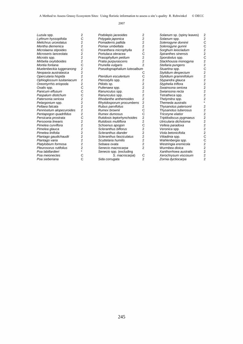
A Method to Assess Grassy Ecosystem Sites: Using floristic information to assess a site’s quality R. Rehwinkel © DECC
2007
245
Luzula spp. 2 Lythrum hyssopifolia C Melichrus urceolatus 2 Mentha diemenica 2 Microlaena stipoides C Microseris lanceolata 2 Microtis spp. 2 Mirbelia oxyloboides 2 Montia fontana C Muelenbeckia tuggeranong 2 Neopaxia australasica 2 Opercularia hispida 2 Ophioglossum lusitaniacum 2 Oreomyrrhis eriopoda 2 Oxalis spp. C Panicum effusum C Paspalum distichum C Patersonia sericea 2 Pelargonium spp. 2 Pellaea falcata 2 Pennisetum alopecuroides 2 Pentapogon quadrifidus 2 Persicaria prostrata C Persoonia linearis 2 Pimelea curviflora 2 Pimelea glauca 2 Pimelea linifolia 2 Plantago gaudichaudii 2 Plantago varia 2 Platylobium formosa 2 Pleurosorus rutifolius 2 Poa labillardieri * Poa meionectes C Poa sieberiana C
Podolepis jaceoides 2 Polygala japonica 2 Pomaderris pallida 2 Pomax umbellata 2 Poranthera microphylla 2 Portulaca oleracea C Prasophyllum petilum 2 Pratia purpurascens 2 Prunella vulgaris 2 Pseudognaphalium luteoalbum
C Pteridium esculentum C Pterostylis spp. 2 Ptilotis sp. 2 Pultenaea spp. 2 Ranunculus spp. 2 Ranunculus spp. 2 Rhodanthe anthemoides 2 Rhytidosporum procumbens 2 Rubus parvifolius 2 Rumex brownii C Rumex dumosus C Rutidosis leptorhynchoides 2 Rutidosis multiflora 2 Schoenus apogon C Scleranthus biflorus 2 Scleranthus diander 2 Scleranthus fasciculatus 2 Scuttelaria humilis 2 Sebaea ovata 2 Senecio macrocarpa 2 Senecio spp. (excluding
S. macrocarpa) C Sida corrugata 2
Solanum sp. (spiny leaves) 2 Solanum spp. 2 Solenogyne dominii C Solenogyne gunnii C Sorghum leiocladum 2 Spiranthes sinensis 2 Sporobolus spp. C Stackhousia monogyna 2 Stellaria pungens 2 Stuartina spp. C Stylidium despectum 2 Stylidium graminifolium 2 Stypandra glauca 2 Styphelia triflora 2 Swainsona sericea 2 Swiansona recta 2 Tetratheca spp. 2 Thelymitra spp. 2 Themeda australis * Thysanotus patersonii 2 Thysanotus tuberosus 2 Tricoryne elatior 2 Triptilodiscus pygmaeus 2 Utricularia dichotoma 2 Velleia paradoxa 2 Veronica spp. 2 Viola betonicifolia 2 Vittadinia spp. C Wahlenbergia spp. C Westringia eremicola 2 Wurmbea dioica 2 Xanthorrhoea australis 2 Xerochrysum viscosum 2 Zornia dyctiocarpa 2

A Method to Assess Grassy Ecosystem Sites: Using floristic information to assess a site’s quality R. Rehwinkel © DECC 2007
246
Appendix 4. Calculation Table (for photocopying)
Site name: Plot ID: Date:
Species name (Native species only)
Braun-Blanquet score
Species type code
Indicator species level 2
Indicator species level 2 with the exception of those with scores of “r”
Indicator species (level 1 & 2)
Indicator species levels 1 & 2 with the exception of those with scores of “r”
XxxxxxxxxxxxxxxxxxxxxxxxxxxxxxxxxxX
See p.9 Appendices Table C Table D Table E Table F
TALLY: XXXxxxxxxxxXXX
XXXxxxxxxxxXXX
XXXxxxxxxxxXXX
SITE’S FLORISTIC VALUE SCORE:
Tally: count, do not total, the number of entries in the required columns: Indicator species level 2 (count all entries), Indicator species level 2 with the exception of those with scores of “r” (count entries with scores greater than “r”), Indicator species levels 1 & 2 with the exception of those with scores of “r” (count entries with scores greater than “r”) To derive a floristic value score for a site, total the three tally numbers along the base of the table.
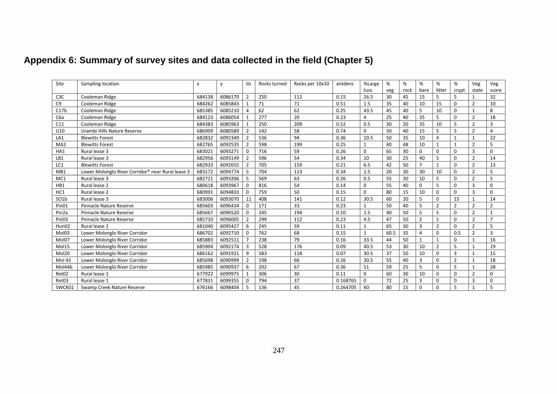
247
Appendix 6: Summary of survey sites and data collected in the field (Chapter 5)
Site Sampling location x y its Rocks turned Rocks per 10x10 antdens %Large tuss
% veg
% rock
% bare
% litter
% crypt
Veg state
Veg score
C3C Cooleman Ridge 684138 6086170 2 250 112 0.15 26.5 30 45 15 5 5 1 32
C9 Cooleman Ridge 684262 6085843 1 71 71 0.51 1.5 35 40 10 15 0 2 10
C17b Cooleman Ridge 685385 6085210 4 62 62 0.25 43.5 45 40 5 10 0 1 8
C6a Cooleman Ridge 684123 6086054 1 277 20 0.23 4 25 40 35 5 0 2 18
C11 Cooleman Ridge 684383 6085963 1 250 209 0.52 0.5 30 20 35 10 5 2 3
U10 Urambi Hills Nature Reserve 686909 6080589 2 142 58 0.74 0 30 40 15 5 5 2 4
LA1 Blewitts Forest 682832 6092349 2 536 94 0.36 10.5 50 35 10 4 1 1 22
MA2 Blewitts Forest 682765 6092535 2 598 199 0.25 1 40 48 10 1 1 2 5
HA1 Rural lease 3 683021 6093271 0 716 59 0.26 0 65 30 0 0 0 3 0
LB1 Rural lease 3 682956 6093149 2 596 54 0.34 10 30 25 40 5 0 2 14
LC1 Blewitts Forest 682933 6092655 2 705 159 0.21 6.5 42 50 7 1 0 2 13
MB1 Lower Molonglo River Corridor* near Rural lease 3 683172 6094774 5 704 113 0.34 1.5 20 30 30 10 0 2 5
MC1 Rural lease 3 682711 6093206 5 569 63 0.26 0.5 55 30 10 5 0 2 5
HB1 Rural lease 2 680618 6093967 0 816 54 0.14 0 55 40 0 5 0 3 0
HC1 Rural lease 2 680991 6094833 0 759 50 0.15 0 80 15 10 0 0 3 0
SO1b Rural lease 3 683006 6093070 11 408 141 0.12 30.5 60 20 5 0 15 1 14
Pin01 Pinnacle Nature Reserve 685603 6096434 0 171 33 0.23 1 50 40 5 2 2 2 2
Pin2a Pinnacle Nature Reserve 685667 6096520 0 245 194 0.10 1.5 40 50 5 5 0 2 1
Pin03 Pinnacle Nature Reserve 685710 6096005 2 299 112 0.23 4.5 47 50 2 1 0 2 7
Hun02 Rural lease 2 681040 6095427 6 245 59 0.11 1 65 30 3 2 0 2 5
Mol03 Lower Molonglo River Corridor 686702 6092710 0 762 68 0.15 1 60.5 35 4 0 0.5 2 3
Mol07 Lower Molonglo River Corridor 685883 6092511 7 238 79 0.16 33.5 44 50 1 1 0 1 16
Mol15 Lower Molonglo River Corridor 685904 6092174 3 528 176 0.09 40.5 53 30 10 2 5 1 19
Mol20 Lower Molonglo River Corridor 686162 6091911 9 583 118 0.07 30.5 37 50 10 0 3 1 15
Mol 43 Lower Molonglo River Corridor 685698 6090999 2 198 66 0.26 30.5 55 40 3 0 2 1 18
Mol44b Lower Molonglo River Corridor 685985 6090937 6 202 67 0.36 51 59 25 5 0 5 1 28
Ret02 Rural lease 1 677922 6099975 1 306 30 0.11 0 60 30 10 0 0 2 0
Ret03 Rural lease 1 677831 6099355 0 794 37 0.168765 0 72 25 3 0 0 3 0
SWCK01 Swamp Creek Nature Reserve 676166 6098404 5 136 45 0.264705 60 80 15 0 0 5 1 5

248
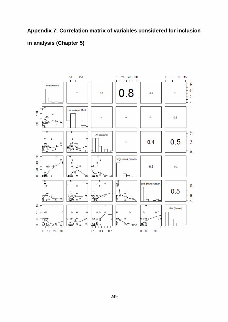
249
Appendix 7: Correlation matrix of variables considered for inclusion
in analysis (Chapter 5)

250
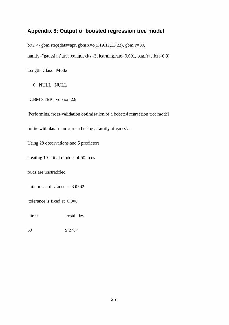
251
Appendix 8: Output of boosted regression tree model
brt2 <- gbm.step(data=apr, gbm.x=c(5,19,12,13,22), gbm.y=30,
family="gaussian",tree.complexity=3, learning.rate=0.001, bag.fraction=0.9)
Length Class Mode
0 NULL NULL
GBM STEP - version 2.9
Performing cross-validation optimisation of a boosted regression tree model
for its with dataframe apr and using a family of gaussian
Using 29 observations and 5 predictors
creating 10 initial models of 50 trees
folds are unstratified
total mean deviance = 8.0262
tolerance is fixed at 0.008
ntrees resid. dev.
50 9.2787
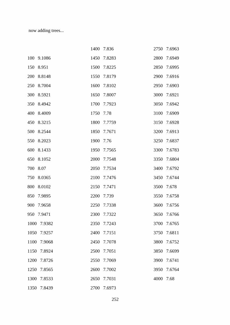
252
now adding trees...
100 9.1086
150 8.951
200 8.8148
250 8.7004
300 8.5921
350 8.4942
400 8.4009
450 8.3215
500 8.2544
550 8.2023
600 8.1433
650 8.1052
700 8.07
750 8.0365
800 8.0102
850 7.9895
900 7.9658
950 7.9471
1000 7.9382
1050 7.9257
1100 7.9068
1150 7.8924
1200 7.8726
1250 7.8565
1300 7.8533
1350 7.8439
1400 7.836
1450 7.8283
1500 7.8225
1550 7.8179
1600 7.8102
1650 7.8007
1700 7.7923
1750 7.78
1800 7.7759
1850 7.7671
1900 7.76
1950 7.7565
2000 7.7548
2050 7.7534
2100 7.7476
2150 7.7471
2200 7.739
2250 7.7338
2300 7.7322
2350 7.7243
2400 7.7151
2450 7.7078
2500 7.7051
2550 7.7069
2600 7.7002
2650 7.7031
2700 7.6973
2750 7.6963
2800 7.6949
2850 7.6995
2900 7.6916
2950 7.6903
3000 7.6921
3050 7.6942
3100 7.6909
3150 7.6928
3200 7.6913
3250 7.6837
3300 7.6783
3350 7.6804
3400 7.6792
3450 7.6744
3500 7.678
3550 7.6758
3600 7.6756
3650 7.6766
3700 7.6765
3750 7.6811
3800 7.6752
3850 7.6699
3900 7.6741
3950 7.6764
4000 7.68
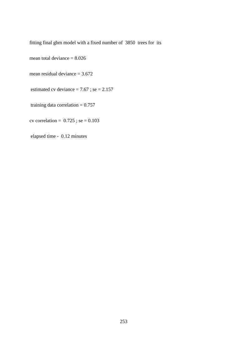
253
fitting final gbm model with a fixed number of 3850 trees for its
mean total deviance = 8.026
mean residual deviance = 3.672
estimated cv deviance = 7.67 ; se = 2.157
training data correlation = 0.757
cv correlation = 0.725 ; se = 0.103
elapsed time - 0.12 minutes
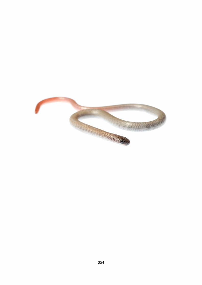
254


![ACT Government - AUSTRALIAN CAPITAL TERRITORY CONTRACT NUMBER: [INSERT] CONTRACT … · 2019. 11. 6. · australian capital territory contract number: [insert] contract name: [insert]](https://img.pdfslide.net/doc/110x75/60aebbf72ac8c7702f4b433a/act-government-australian-capital-territory-contract-number-insert-contract.jpg)