Embed Size (px)
DESCRIPTION
Nearest-neighbor and Bilinear Resampling Factor Estimation to Detect Blockiness or Blurriness of an Image*. Ariawan Suwendi Prof. Jan P. Allebach Purdue University - West Lafayette, IN. *Research supported by the Hewlett-Packard Company. Outline. Introduction - PowerPoint PPT Presentation
Citation preview
EI 2006 - San Jose, CA Slide No. 1
Nearest-neighbor and Bilinear Resampling Factor Estimation to
Detect Blockiness or Blurriness of an Image*
Ariawan Suwendi
Prof. Jan P. Allebach
Purdue University - West Lafayette, IN
*Research supported by the Hewlett-Packard Company
EI 2006 - San Jose, CA Slide No. 2
Outline
Introduction
1-D Nearest-neighbor and bilinear interpolation
The basis for interpolation detection (RF>1)
Step-by-step illustration of the resampling factor estimation
algorithm
Robustness evaluation
Conclusions
EI 2006 - San Jose, CA Slide No. 3
Introduction
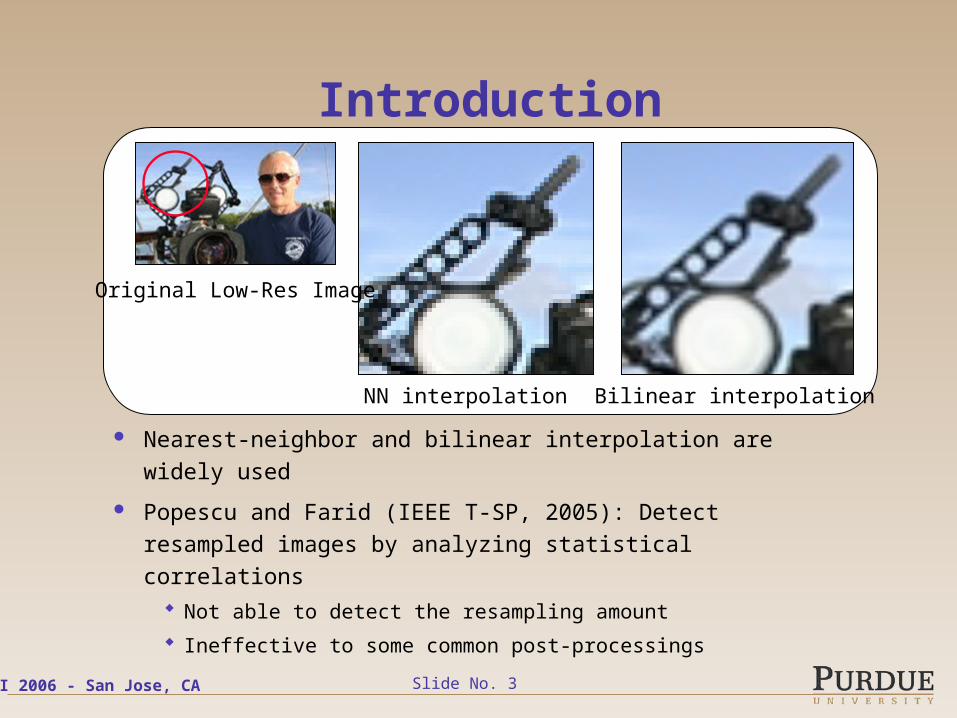
Nearest-neighbor and bilinear interpolation are widely
used
Popescu and Farid (IEEE T-SP, 2005): Detect resampled
images by analyzing statistical correlations
Not able to detect the resampling amount
Ineffective to some common post-processings
Original Low-Res Image
NN interpolation Bilinear interpolation
EI 2006 - San Jose, CA Slide No. 4
Introduction (cont.)
How to detect and estimate resampling factor (RF) for
nearest-neighbor and bilinear interpolation
Since both interpolations are separable, most of the things
will be explained in 1-D space
EI 2006 - San Jose, CA Slide No. 5
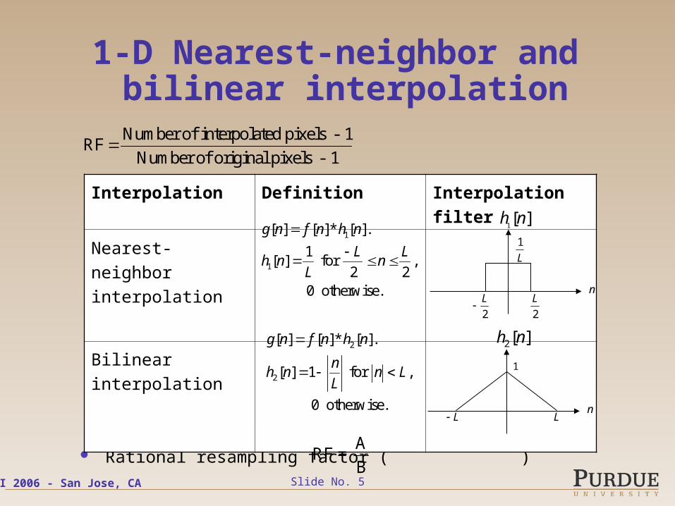
1-D Nearest-neighbor and bilinear interpolation
Rational resampling factor ( )
Number of interpolated pixels - 1RF
Number of original pixels - 1
Interpolation Definition Interpolation filter
Nearest-neighbor
interpolation
Bilinear interpolation
1
L L
2[ ]h n
n
1
L
2
L
2
L
1[ ]h n
n
1
1
[ ] [ ]* [ ].
1[ ] for ,
2 2 0 otherwise.
g n f n h n
L Lh n n
L
2
2
[ ] [ ]* [ ].
[ ] 1 for ,
0 otherwise.
g n f n h n
nh n n L
L
ARF =
B
EI 2006 - San Jose, CA Slide No. 6
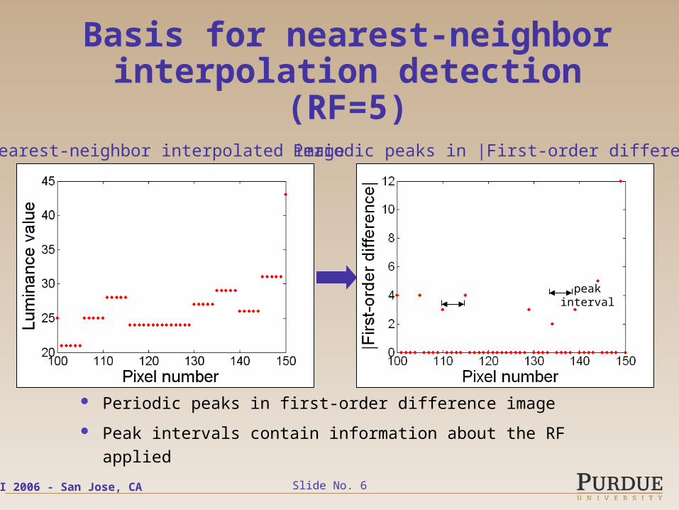
Basis for nearest-neighbor interpolation detection (RF=5)
Periodic peaks in first-order difference image
Peak intervals contain information about the RF applied
Nearest-neighbor interpolated image Periodic peaks in |First-order difference|
peakinterval
EI 2006 - San Jose, CA Slide No. 7
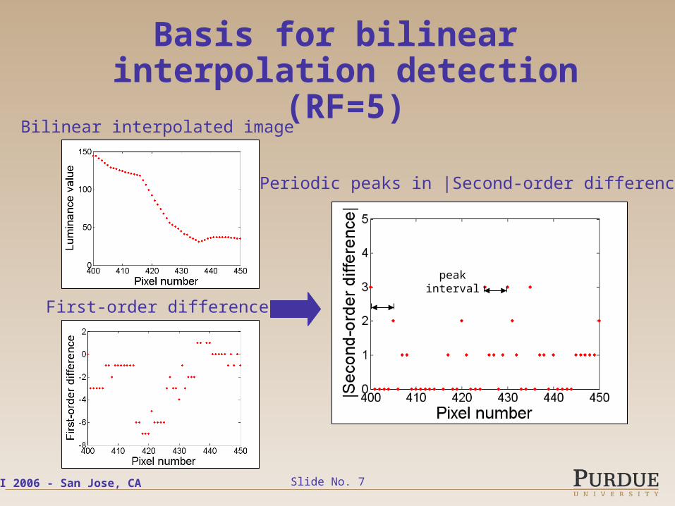
Basis for bilinear interpolation detection (RF=5)
Bilinear interpolated image
First-order difference
Periodic peaks in |Second-order difference|
peakinterval
EI 2006 - San Jose, CA Slide No. 8
Basis for interpolation detection
In nearest-neighbor interpolated images, the first-order difference image should contain peaks with peak intervals equal floor(RF) or ceil(RF)
In bilinear interpolated images, the second-order difference image should contain peaks with peak intervals equal floor(RF) or ceil(RF)
Resampling factor RF can be estimated as the average of the detected peak intervals
Smooth regions in the difference image do not provide a reliable reading of peak intervals and, hence, should be ignored
EI 2006 - San Jose, CA Slide No. 9
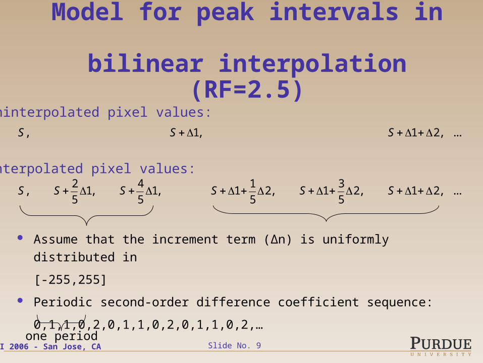
Model for peak intervals in bilinear interpolation (RF=2.5)
, 1, 1 2, ...
2 4 1 3, 1, 1, 1 2, 1 2, 1 2, ...
5 5 5 5
S S S
S S S S S S
Uninterpolated pixel values:
Interpolated pixel values:
Assume that the increment term (Δn) is uniformly distributed in
[-255,255]
Periodic second-order difference coefficient sequence:
0,1,1,0,2,0,1,1,0,2,0,1,1,0,2,…
one period
EI 2006 - San Jose, CA Slide No. 10
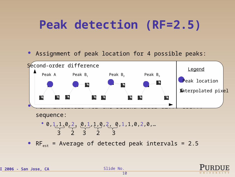
Peak detection (RF=2.5)
Assignment of peak location for 4 possible peaks:
Peak intervals for the second-order diff. coeff. sequence:
0,1,1,0,2, 0,1,1,0,2, 0,1,1,0,2,0,…
RFest = Average of detected peak intervals = 2.5
3 2 3 2 3
Peak location
Interpolated pixel
LegendSecond-order difference
Peak A Peak B1 Peak B2 Peak B3
EI 2006 - San Jose, CA Slide No. 11
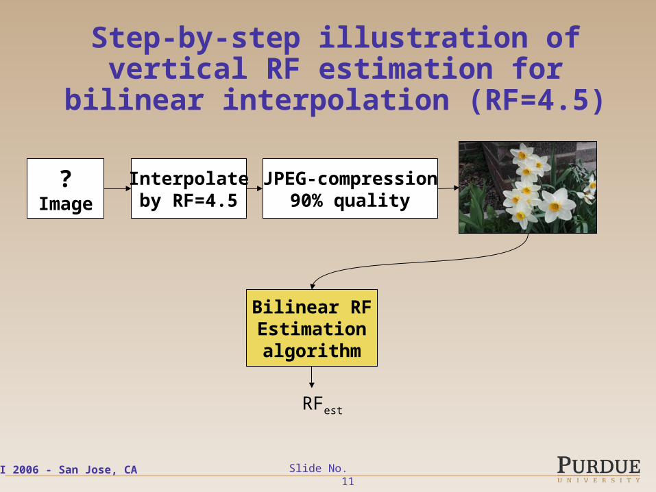
Step-by-step illustration of vertical RF estimation for bilinear interpolation
(RF=4.5)
?Image
Interpolateby RF=4.5
JPEG-compression90% quality
Bilinear RFEstimationalgorithm
RFest
EI 2006 - San Jose, CA Slide No. 12
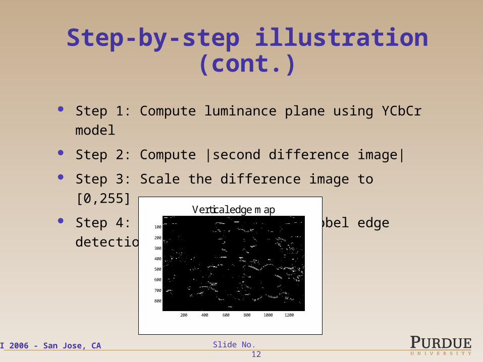
Step-by-step illustration (cont.)
Step 1: Compute luminance plane using YCbCr model
Step 2: Compute |second difference image|
Step 3: Scale the difference image to [0,255]
Step 4: Apply the horizontal Sobel edge detection filter
Vertical edge map
200 400 600 800 1000 1200
100
200
300
400
500
600
700
800
EI 2006 - San Jose, CA Slide No. 13
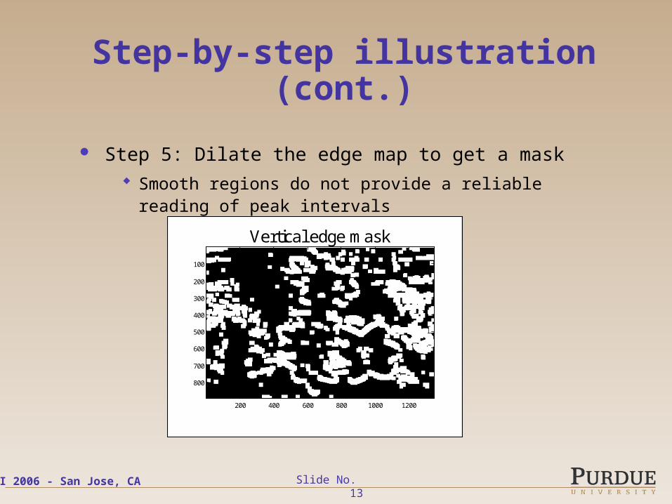
Step-by-step illustration (cont.)
Step 5: Dilate the edge map to get a mask
Smooth regions do not provide a reliable reading of peak intervals
Vertical edge mask
200 400 600 800 1000 1200
100
200
300
400
500
600
700
800
EI 2006 - San Jose, CA Slide No. 14
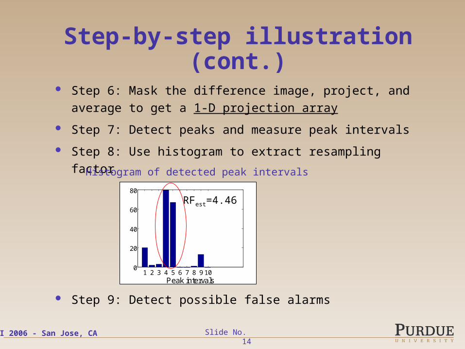
Step-by-step illustration (cont.)
Step 6: Mask the difference image, project, and average to
get a 1-D projection array
Step 7: Detect peaks and measure peak intervals
Step 8: Use histogram to extract resampling factor
Step 9: Detect possible false alarms
1 2 3 4 5 6 7 8 9 100
20
40
60
80
Peak intervals
RFest=4.46
Histogram of detected peak intervals
EI 2006 - San Jose, CA Slide No. 15
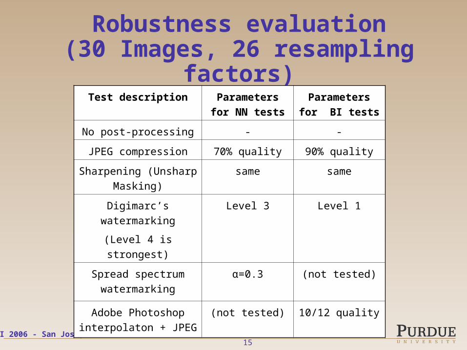
Robustness evaluation(30 Images, 26 resampling factors)
Test description Parameters for
NN tests
Parameters for
BI tests
No post-processing - -
JPEG compression 70% quality 90% quality
Sharpening (Unsharp
Masking)
same same
Digimarc’s watermarking
(Level 4 is strongest)
Level 3 Level 1
Spread spectrum
watermarking
α=0.3 (not tested)
Adobe Photoshop
interpolaton + JPEG
(not tested) 10/12 quality
EI 2006 - San Jose, CA Slide No. 16
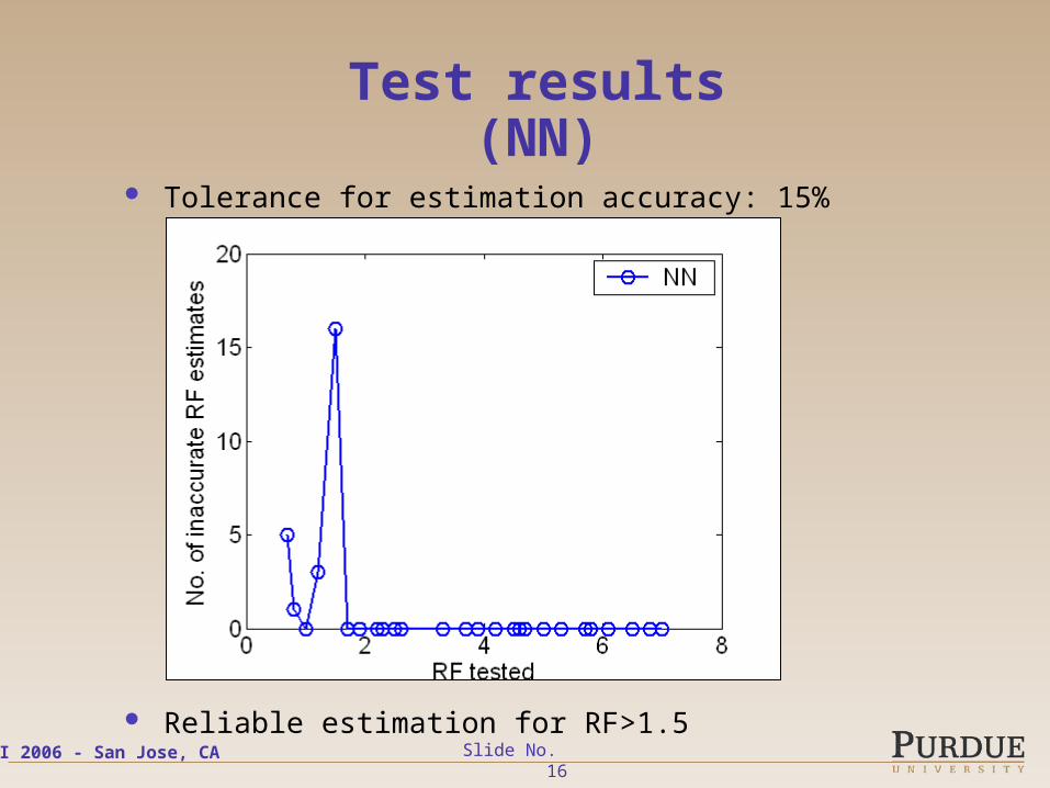
Test results(NN)
Tolerance for estimation accuracy: 15%
Reliable estimation for RF>1.5
EI 2006 - San Jose, CA Slide No. 17
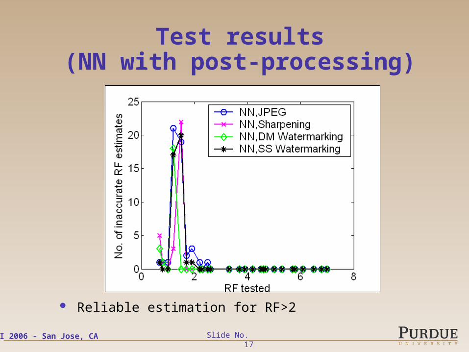
Test results(NN with post-processing)
Reliable estimation for RF>2
EI 2006 - San Jose, CA Slide No. 18
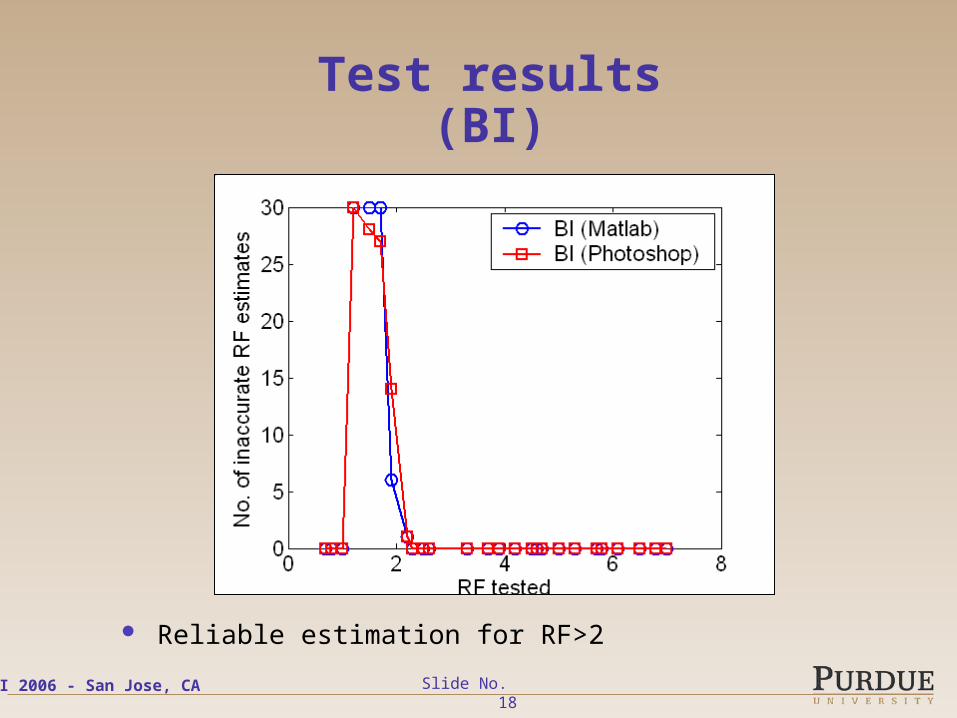
Test results(BI)
Reliable estimation for RF>2
EI 2006 - San Jose, CA Slide No. 19
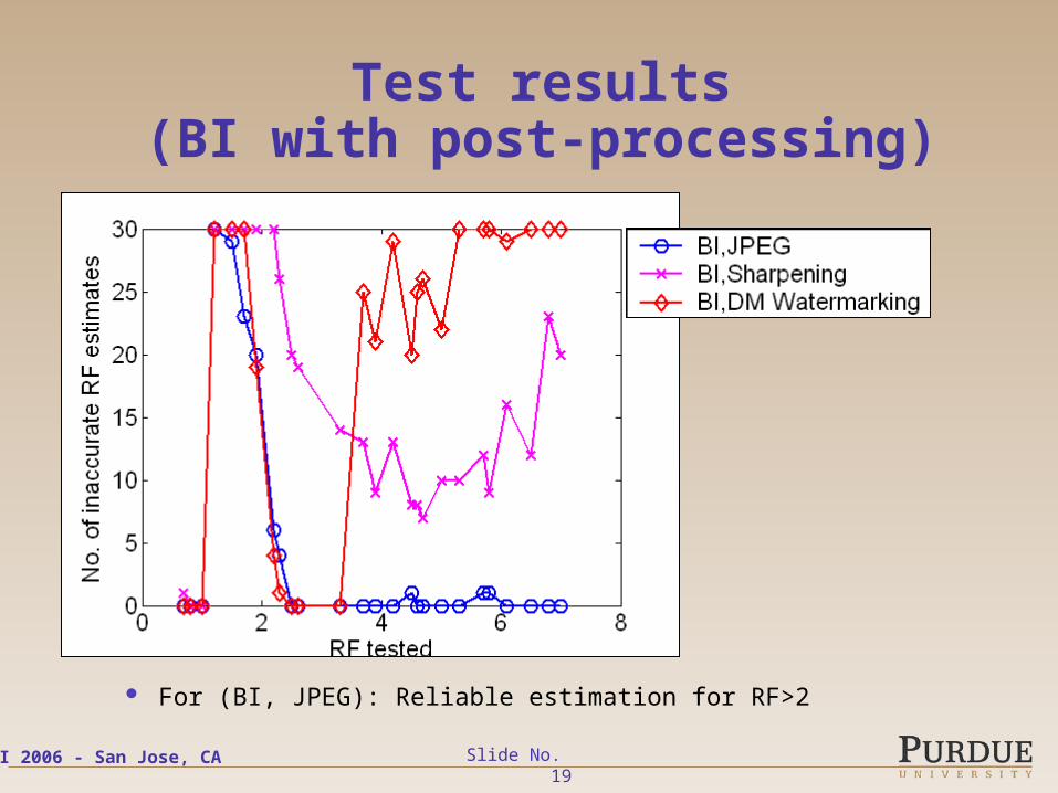
Test results(BI with post-processing)
For (BI, JPEG): Reliable estimation for RF>2
EI 2006 - San Jose, CA Slide No. 20
Conclusions
The NN resampling factor estimation algorithm works well
for RF>2
It can withstand significant post-processing
The bilinear resampling factor estimation algorithm works
well for RF>2 except in sharpening and watermarking tests
It can only withstand mild post-processing
One weakness is that bilinear interpolation with 1<RF<2
tends to be overestimated with 2<RFest≤3
EI 2006 - San Jose, CA Slide No. 21
Thank you for listening