Embed Size (px)
Citation preview
ArtiSynth: A Fast Interactive BiomechanicalModeling Toolkit Combining Multibody andFinite Element Simulation
John E. Lloyd, Ian Stavness, and Sidney Fels
Abstract ArtiSynth (www.artisynth.org) is an open source, Java-based biome-chanical simulation environment for modeling complex anatomical systems com-posed of both rigid and deformable structures. Models can be built from a rich setof components, including particles, rigid bodies, finite elements with both linearand nonlinear materials, point-to-point muscles, and various bilateral and unilateralconstraints including contact. A state-of-the-art physics simulator provides forwardsimulation capabilities that combine multibody and finite element models. Inversesimulation capabilities allow the computation of the muscle activations needed toachieve prescribed target motions. ArtiSynth is highly interactive, with componentparameters and state variables exposed as properties that can be interactively readand adjusted as the simulation proceeds. Streams of input and output data, usedfor controlling or observing the simulation, can be viewed, arranged, and edited onan interactive timeline display, and support is provided for the graphical editing ofmodel structures.
1 Introduction
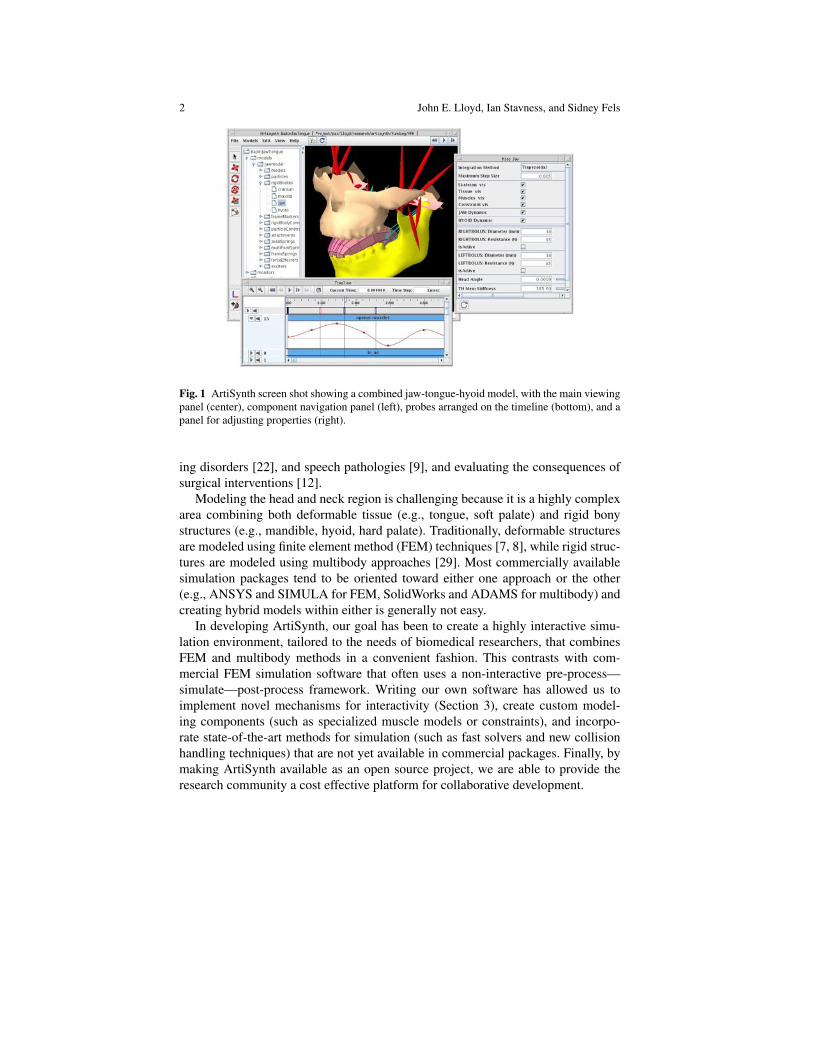
The ArtiSynth modeling platform has been developed at the University of BritishColumbia for the past several years. Originally created for modeling the mechanicsof speech production, the system has evolved into a general biomechanical simu-lation environment, with most usage to date focussed on modeling the head andneck region for research in physiology, medicine, dentistry, and linguistics (Figure1). Many applications are directed toward understanding and treating pathologies ofthe oral cavity and upper airway, including obstructive sleep apnea [19], swallow-
Lloyd and Fels: Department of Electrical and Computer EngineeringUniversity of British Columbia, e-mail: [email protected],[email protected]
Stavness: Department of BioengineeringStanford University, e-mail: [email protected]
1
2 John E. Lloyd, Ian Stavness, and Sidney Fels
Fig. 1 ArtiSynth screen shot showing a combined jaw-tongue-hyoid model, with the main viewingpanel (center), component navigation panel (left), probes arranged on the timeline (bottom), and apanel for adjusting properties (right).
ing disorders [22], and speech pathologies [9], and evaluating the consequences ofsurgical interventions [12].
Modeling the head and neck region is challenging because it is a highly complexarea combining both deformable tissue (e.g., tongue, soft palate) and rigid bonystructures (e.g., mandible, hyoid, hard palate). Traditionally, deformable structuresare modeled using finite element method (FEM) techniques [7, 8], while rigid struc-tures are modeled using multibody approaches [29]. Most commercially availablesimulation packages tend to be oriented toward either one approach or the other(e.g., ANSYS and SIMULA for FEM, SolidWorks and ADAMS for multibody) andcreating hybrid models within either is generally not easy.
In developing ArtiSynth, our goal has been to create a highly interactive simu-lation environment, tailored to the needs of biomedical researchers, that combinesFEM and multibody methods in a convenient fashion. This contrasts with com-mercial FEM simulation software that often uses a non-interactive pre-process—simulate—post-process framework. Writing our own software has allowed us toimplement novel mechanisms for interactivity (Section 3), create custom model-ing components (such as specialized muscle models or constraints), and incorpo-rate state-of-the-art methods for simulation (such as fast solvers and new collisionhandling techniques) that are not yet available in commercial packages. Finally, bymaking ArtiSynth available as an open source project, we are able to provide theresearch community a cost effective platform for collaborative development.
ArtiSynth: A Fast Interactive Biomechanical Modeling Toolkit 3
Key features of ArtiSynth include:
• A comprehensive API for creating and interconnecting anatomical models fromrigid bodies, joints, finite element models, point-to-point muscles (including Hilland other types), particles, etc.
• Tetrahedral, hexahedral, and higher-order FEM elements, along with materialsincluding co-rotated linear, hyperelastic, viscoelastic, and transverse isotropic.
• Fast simulation using state-of-the-art physics simulation that handles bilateraland unilateral constraints, contact and friction.
• Inverse simulation capabilities to determine the muscle activations required toachieve particular tasks.
• A Jython console for dynamic interaction and scripting.• A highly interactive environment, with GUI support for setting properties, trans-
forming and editing structure, and viewing and editing input and output data ona timeline.
• Extensibility, with the ability to easily add custom and special purpose compo-nents or override aspects of the simulation behavior.
Other open source systems for biomechanics have been developed in recentyears. These include: OpenSim [15], which provides a highly accurate multibodysimulator and lumped line-based muscle models for performing musculoskeletalanalysis; FEBio [26], a finite element package that uses a traditional pre-process—simulate—post-process framework with special support for tissue modeling andsome support for rigid bodies, contact and constraints. Systems geared toward sur-gical training include Gipsi [11] and Spring [24]. Sofa [2] provides a general soft-ware architecture in which models can be partitioned into different sub-models forsimulating appearance, behavior, and/or haptic response. ArtiSynth and Sofa bothprovide the ability to combine multibody and FEM models, with Sofa targetedmore towards realtime applications such as surgical simulation and ArtiSynth di-rected more towards precise physiological modeling. Sofa uses a very general scene-graph arrangement for creating models, while ArtiSynth employs a more traditionalcomponent-based approach. ArtiSynth also supplies a comprehensive simulation en-gine (Section 4) that can solve any Lagrangian based mechanical system containingboth bilateral and unilateral constraints.
The remainder of this chapter is organized as follows. An overview of ArtiSynth’sdesign is given in Section 2, followed by a description of the user interactivity fea-tures (Section 3), the forward-dynamics physics simulation (Section 4), and inversesimulation capabilities (Section 5). Section 6 gives a concise overview of some ofthe models that have been created to date, and concluding remarks and a discussionof future work is given in Section 7.
4 John E. Lloyd, Ian Stavness, and Sidney Fels
2 General System Design
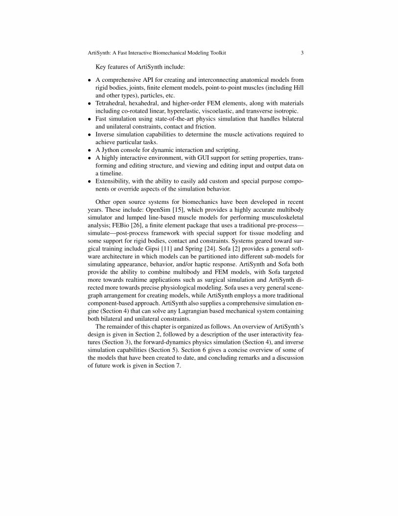
A primary design goal of ArtiSynth is to provide the user with comprehensive in-teractive simulation control, which is achieved using a rich graphical user interface(GUI). Figure 2 provides a overview schematic of the system’s organization. At thecenter are the models, composed of a hierarchy of components. The GUI allows auser to view and edit the model hierarchy, using one or more OpenGL-based view-ers, along with selection, navigation, and editing tools that allow components to beadded, modified, or deleted. The properties of selected components can be modifiedusing property panels. Play controls allow simulation to be started, paused, singlestepped, or reset. Simulation proceeds under the control of a scheduler, which co-ordinates the actions of the a physics simulator that advances the models throughtime. Streams of input and output data (known as probes) can be attached to themodel to control or observe the simulation as it proceeds. Typically, input probedata consists of external forces, muscle activation levels, or kinematically specifiedmotions, while output probe data contains simulation results such as positions, ve-locities, muscle forces, or reaction forces. Probes and their data can be observed,edited, and temporally arranged using a GUI timeline component. Applications canalso add controllers to preprocess and provide control inputs at the beginning ofeach time step, as well as monitors to collect and post-process observed data at theend of each time step.
Physicssimulation
Model hierarchy
Timeline
GUI
Viewers & edit tools
Property panels
SchedulerPlay controls
Input data Output data Probes
Controllers Monitors
Fig. 2 General organization of the ArtiSynth system.
ArtiSynth: A Fast Interactive Biomechanical Modeling Toolkit 5
2.1 Java implementation and basic component classes
ArtiSynth is implemented in Java. This decision was made to facilitate portability,particularly for the graphical interface, across various system platforms. While Javais slower than other languages (typically by a factor of two for optimized code afterjust-in-time compilation), this is not too problematic since the major computationalbottleneck is usually the linear solves required by the physics simulator (Section 4).These linear solves, in turn, are done using direct solvers compiled in native code.
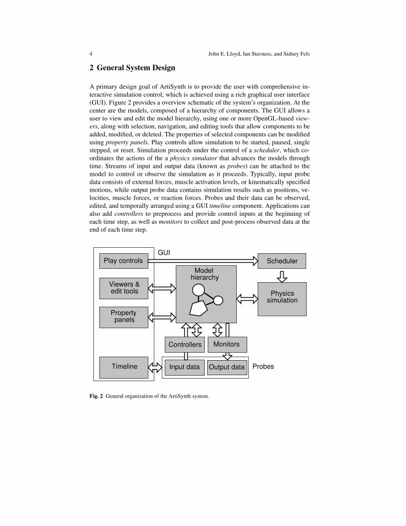
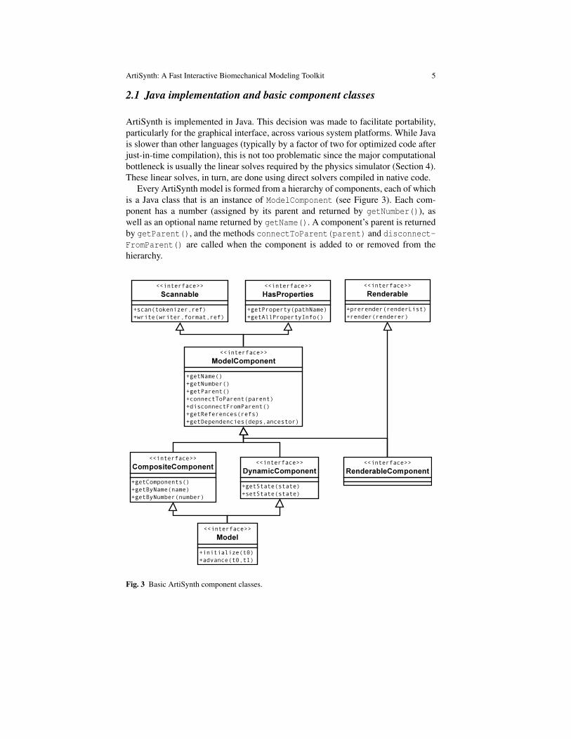
Every ArtiSynth model is formed from a hierarchy of components, each of whichis a Java class that is an instance of ModelComponent (see Figure 3). Each com-ponent has a number (assigned by its parent and returned by getNumber()), aswell as an optional name returned by getName(). A component’s parent is returnedby getParent(), and the methods connectToParent(parent) and disconnect-FromParent() are called when the component is added to or removed from thehierarchy.
Fig. 3 Basic ArtiSynth component classes.
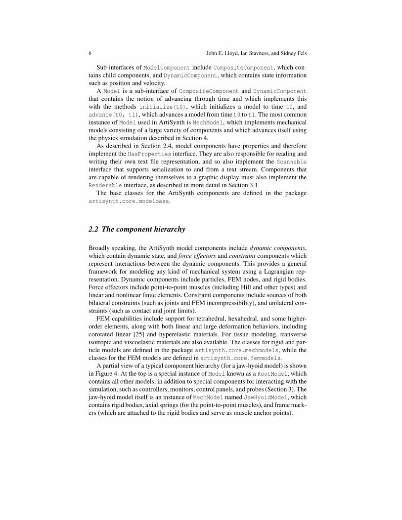
6 John E. Lloyd, Ian Stavness, and Sidney Fels
Sub-interfaces of ModelComponent include CompositeComponent, which con-tains child components, and DynamicComponent, which contains state informationsuch as position and velocity.
A Model is a sub-interface of CompositeComponent and DynamicComponentthat contains the notion of advancing through time and which implements thiswith the methods initialize(t0), which initializes a model to time t0, andadvance(t0, t1), which advances a model from time t0 to t1. The most commoninstance of Model used in ArtiSynth is MechModel, which implements mechanicalmodels consisting of a large variety of components and which advances itself usingthe physics simulation described in Section 4.
As described in Section 2.4, model components have properties and thereforeimplement the HasProperties interface. They are also responsible for reading andwriting their own text file representation, and so also implement the Scannableinterface that supports serialization to and from a text stream. Components thatare capable of rendering themselves to a graphic display must also implement theRenderable interface, as described in more detail in Section 3.1.
The base classes for the ArtiSynth components are defined in the packageartisynth.core.modelbase.
2.2 The component hierarchy
Broadly speaking, the ArtiSynth model components include dynamic components,which contain dynamic state, and force effectors and constraint components whichrepresent interactions between the dynamic components. This provides a generalframework for modeling any kind of mechanical system using a Lagrangian rep-resentation. Dynamic components include particles, FEM nodes, and rigid bodies.Force effectors include point-to-point muscles (including Hill and other types) andlinear and nonlinear finite elements. Constraint components include sources of bothbilateral constraints (such as joints and FEM incompressibility), and unilateral con-straints (such as contact and joint limits).
FEM capabilities include support for tetrahedral, hexahedral, and some higher-order elements, along with both linear and large deformation behaviors, includingcorotated linear [25] and hyperelastic materials. For tissue modeling, transverseisotropic and viscoelastic materials are also available. The classes for rigid and par-ticle models are defined in the package artisynth.core.mechmodels, while theclasses for the FEM models are defined in artisynth.core.femmodels.
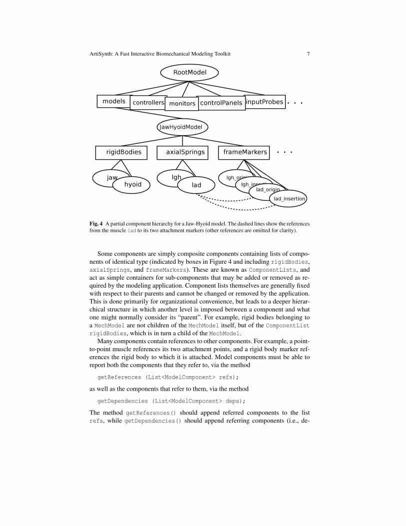
A partial view of a typical component hierarchy (for a jaw-hyoid model) is shownin Figure 4. At the top is a special instance of Model known as a RootModel, whichcontains all other models, in addition to special components for interacting with thesimulation, such as controllers, monitors, control panels, and probes (Section 3). Thejaw-hyoid model itself is an instance of MechModel named JawHyoidModel, whichcontains rigid bodies, axial springs (for the point-to-point muscles), and frame mark-ers (which are attached to the rigid bodies and serve as muscle anchor points).
ArtiSynth: A Fast Interactive Biomechanical Modeling Toolkit 7
Fig. 4 A partial component hierarchy for a Jaw-Hyoid model. The dashed lines show the referencesfrom the muscle lad to its two attachment markers (other references are omitted for clarity).
Some components are simply composite components containing lists of compo-nents of identical type (indicated by boxes in Figure 4 and including rigidBodies,axialSprings, and frameMarkers). These are known as ComponentLists, andact as simple containers for sub-components that may be added or removed as re-quired by the modeling application. Component lists themselves are generally fixedwith respect to their parents and cannot be changed or removed by the application.This is done primarily for organizational convenience, but leads to a deeper hierar-chical structure in which another level is imposed between a component and whatone might normally consider its “parent”. For example, rigid bodies belonging toa MechModel are not children of the MechModel itself, but of the ComponentListrigidBodies, which is in turn a child of the MechModel.
Many components contain references to other components. For example, a point-to-point muscle references its two attachment points, and a rigid body marker ref-erences the rigid body to which it is attached. Model components must be able toreport both the components that they refer to, via the method
getReferences (List<ModelComponent> refs);
as well as the components that refer to them, via the method
getDependencies (List<ModelComponent> deps);
The method getReferences() should append referred components to the listrefs, while getDependencies() should append referring components (i.e., de-
8 John E. Lloyd, Ian Stavness, and Sidney Fels
pendencies) to deps. Both getReferences() and getDependencies() are usedby the structural editing software described in Section 3.6. A component’s internalstructures which keep track of references and dependencies should be updated inconnectToParent() and disconnectFromParent() when components are con-nected and disconnected from the hierarchy.
The names and/or numbers of a component and its ancestors can be used to forma component path name. This path has a construction analogous to Unix file pathnames, with the ’/’ character acting as a separator. Absolute paths start with ’/’ andbegin above the root model. Relative paths omit the leading ’/’ and can begin lowerdown in the hierarchy. The absolute path name of the axial spring lad in Figure 4would be
/RootModel/models/JawHyoidModel/axialSprings/lad
A component can also be addressed by its number (returned by getNumber(), sothat even nameless components always have a valid path name. For example, the theaxial spring lad could also be addressed by the path name
/0/0/1/1
although this would be most likely to appear only in machine-generated output. Acomponent’s number is assigned when it is added to its parent, and that numberpersists until the component is removed, ensuring that path names remain valid aslong as a component is connected to the hierarchy.
2.3 Model creation
At present, ArtiSynth models are usually created in code, typically by declaring asubclass of the top level RootModel (described above) and then using its constructorto create the remainder of the component hierarchy. In this sense, the Java code takesthe role of a script that creates the various model components and assembles them.This idea is used in other systems, such as the .mac file format of ANSYS, which isessentially a scripting language.
There are several reasons for creating models in code. First, it tends to be morerepeatable, more precise, and (for complex models) easier that using a GUI. Second,models often require specialized code and classes, which cannot be specified easilyin a file format.
Biomechanical models will usually contain at least one instance of MechModel,which itself provides methods for adding sub-components in a straightforward fash-ion. A code fragment to construct the portion of the model hierarchy shown in Figure4 is:
MechModel jawHyoid = new MechModel ("JawHyoidModel");RigidBody jaw = RigidBody.createFromMesh (
"jaw", "jawMesh.obj", 1000, 1);RigidBody hyoid = RigidBody.createFromMesh (
ArtiSynth: A Fast Interactive Biomechanical Modeling Toolkit 9
"hyoid", "hyoidMesh.obj", 1000, 1);
jawHyoid.addRigidBody (jaw);jawHyoid.addRigidBody (hyoid);
Muscle lgh = Muscle.createPeck ("lgh", 40, 35, 45, 0.0);
FrameMarker lghOrigin = new FrameMarker("lgh_origin");FrameMarker lghInsertion = new FrameMarker("lgh_insertion");
jawHyoid.addFrameMarker (lghInsertion, hyoid, new Point3d ( 0.99, 1.69, 7.12));
jawHyoid.addFrameMarker (lghOrigin, jaw, new Point3d ( 1.99, -33.16, 14.74));
jawHyoid.attachAxialSpring (lghOrigin, lghInsertion, lgh);
addModel (jawHyoid);
First, an instance of MechModel, named JawHyoidModel, is created. The jaw andhyoid rigid bodies are then generated using createFromMesh(), which is a conve-nience routine that creates rigid bodies given a name, a mesh file, a density, and ascale factor. These are then added to the jaw-hyoid model using addRigidBody(),which inserts them into the rigidBodies component list. The muscle lgh is cre-ated next, using the convenience routine createPeck() that assigns names andparameters. Two FrameMarker components are then generated to act as the ori-gin and insertion points for the lgh muscle on the jaw and hyoid, and are addedto the model using addFrameMarker(), which attaches a marker to a particularrigid body at a particular location. Finally, the muscle is added to the model usingattachAxialSpring(), which connects it to the specified attachment points andinserts it into the axialSpring list, and the model itself is added to the RootModelusing addModel().
As suggested in the above example, model construction code often makes exten-sive use of geometric file formats. Surface meshes are often used to describe rigidbodies and can be read in from Alias Wavefront .obj files. Similarly, finite ele-ment models can be specified using volumetric meshes read in from either Tetgenor ANSYS .node and .elem files.
Once the model generation code has been written and compiled, it can be loadedinto ArtiSynth by specifying the name of the RootModel subclass in the GUI.A direct way to do this is to choose "Load from class" from the File menu,which invokes a dialog allowing the class to be specified. Alternatively, a specificset of RootModel classes may be assigned “demo” names in the configuration file.demoModels (located in any directory specified the user’s ARTISYNTH PATH envi-ronment variable), using entries that look like:
"Spring Mesh" artisynth.models.mechdemos.SpringMeshDemo
10 John E. Lloyd, Ian Stavness, and Sidney Fels
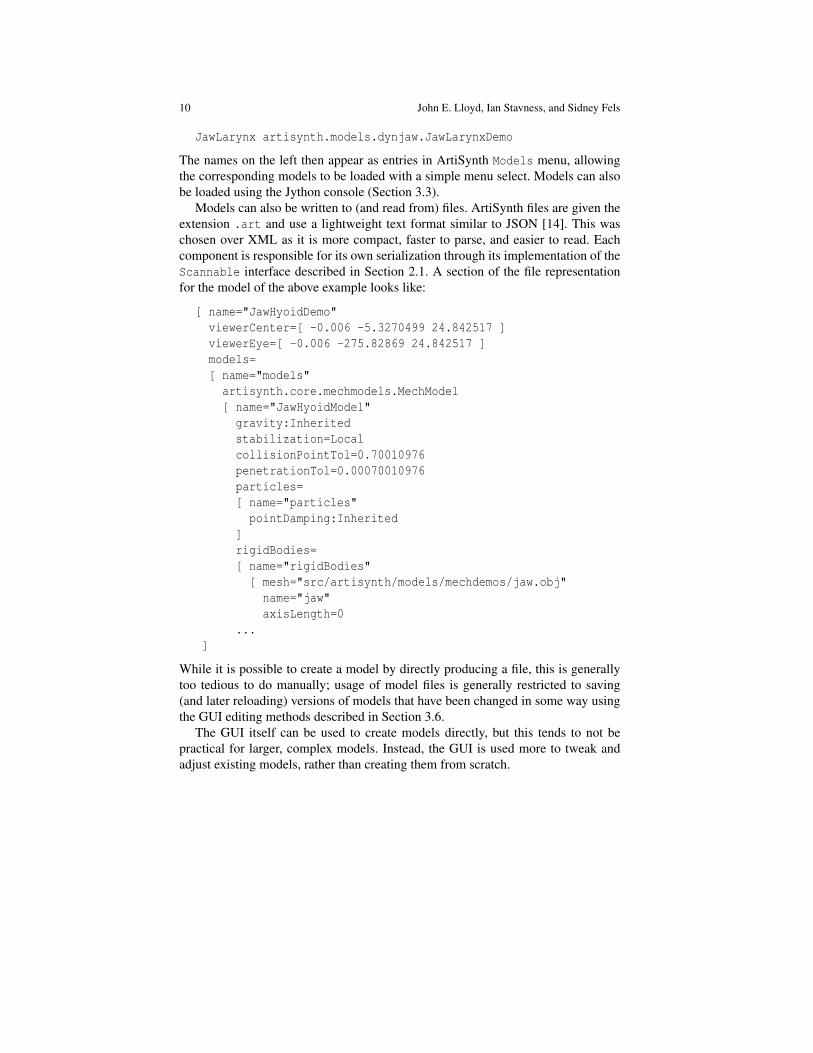
JawLarynx artisynth.models.dynjaw.JawLarynxDemo
The names on the left then appear as entries in ArtiSynth Models menu, allowingthe corresponding models to be loaded with a simple menu select. Models can alsobe loaded using the Jython console (Section 3.3).
Models can also be written to (and read from) files. ArtiSynth files are given theextension .art and use a lightweight text format similar to JSON [14]. This waschosen over XML as it is more compact, faster to parse, and easier to read. Eachcomponent is responsible for its own serialization through its implementation of theScannable interface described in Section 2.1. A section of the file representationfor the model of the above example looks like:
[ name="JawHyoidDemo"viewerCenter=[ -0.006 -5.3270499 24.842517 ]viewerEye=[ -0.006 -275.82869 24.842517 ]models=[ name="models"
artisynth.core.mechmodels.MechModel[ name="JawHyoidModel"gravity:Inheritedstabilization=LocalcollisionPointTol=0.70010976penetrationTol=0.00070010976particles=[ name="particles"
pointDamping:Inherited]rigidBodies=[ name="rigidBodies"
[ mesh="src/artisynth/models/mechdemos/jaw.obj"name="jaw"axisLength=0
...]
While it is possible to create a model by directly producing a file, this is generallytoo tedious to do manually; usage of model files is generally restricted to saving(and later reloading) versions of models that have been changed in some way usingthe GUI editing methods described in Section 3.6.
The GUI itself can be used to create models directly, but this tends to not bepractical for larger, complex models. Instead, the GUI is used more to tweak andadjust existing models, rather than creating them from scratch.
ArtiSynth: A Fast Interactive Biomechanical Modeling Toolkit 11
2.4 Properties
ArtiSynth components expose properties, which provide a uniform interface for ac-cessing their internal parameters and state. Properties vary from component to com-ponent; those for RigidBody include position, orientation, mass, and density,while those for Muscle include maxForce, excitation, and damping. Propertiesare extremely useful for automatically creating GUI widgets and input and outputprobes (Section 2.5). They are also useful in automating component serialization.
Each ArtiSynth component implements HasProperties, which is defined as
interface HasProperties{
Property getProperty (String name);PropertyInfoList getAllPropertyInfo ();
}
The method getProperty() returns a Property handle for the named property,while getAllPropertyInfo() returns information for all properties exposed bythe class. A Property handle, in turn, is defined as
interface Property{
Object get();void set (Object value);Object validate (Object value, StringHolder errMsg);HasProperties getHost();PropertyInfo getInfo();
}
where get() and set() access the property’s value, validate() can be used todetermine if a specific value is valid, getHost() returns the component object towhich the property belongs, and getInfo() returns detailed information about theproperty.
The code fragment below shows how to use the property interface to obtain thecurrent excitation value for a Muscle:
Muscle muscle;...Property prop = muscle.getProperty ("excitation");double excitation = (Double)prop.get();
Note, however, that properties are mostly used by generic system code; in an appli-cation, the above would more be likely be written directly as
double excitation = muscle.getExcitation();
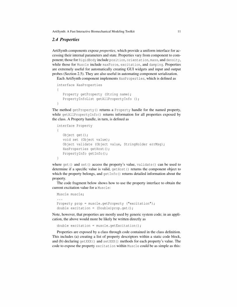
Properties are exposed by a class through code contained in the class definition.This includes (a) creating a list of property descriptors within a static code block,and (b) declaring getXXX() and setXXX() methods for each property’s value. Thecode to expose the property excitation within Muscle could be as simple as this:
12 John E. Lloyd, Ian Stavness, and Sidney Fels
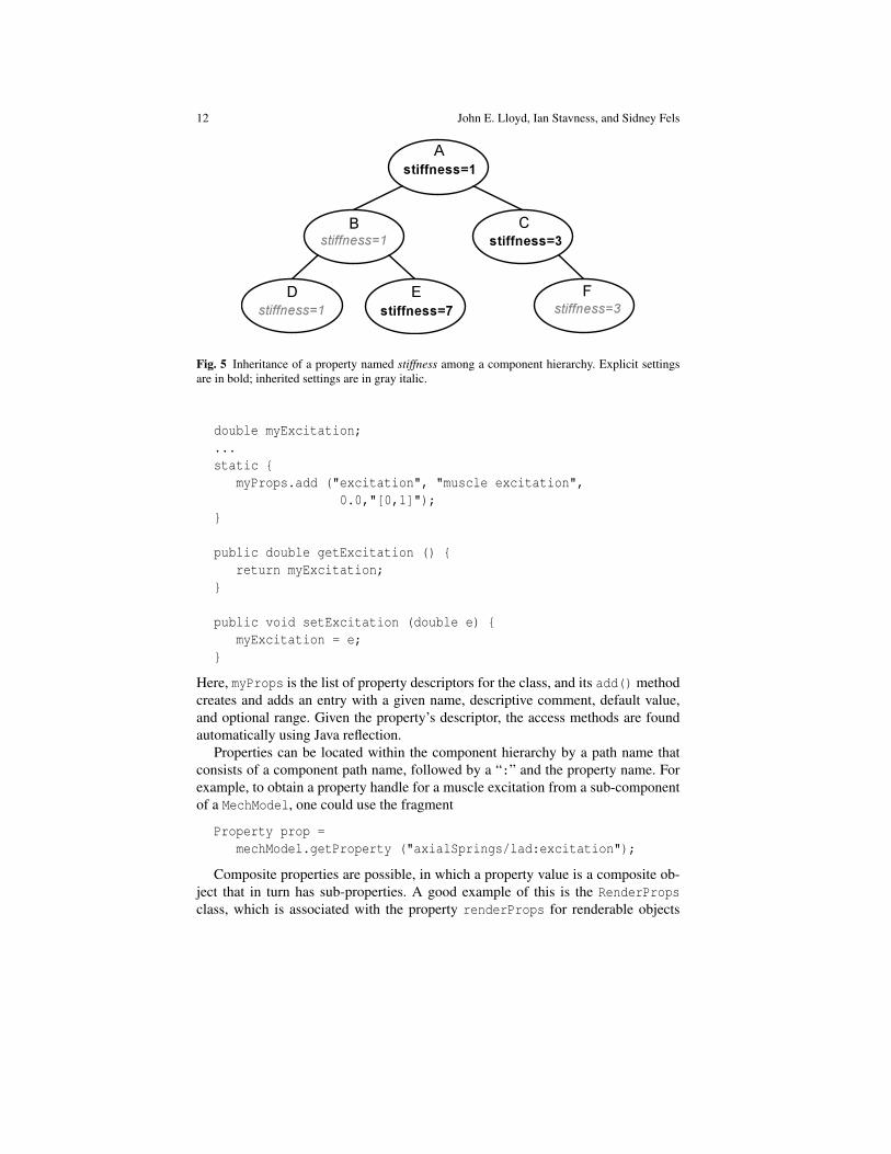
Fig. 5 Inheritance of a property named stiffness among a component hierarchy. Explicit settingsare in bold; inherited settings are in gray italic.
double myExcitation;...static {
myProps.add ("excitation", "muscle excitation",0.0,"[0,1]");
}
public double getExcitation () {return myExcitation;
}
public void setExcitation (double e) {myExcitation = e;
}
Here, myProps is the list of property descriptors for the class, and its add() methodcreates and adds an entry with a given name, descriptive comment, default value,and optional range. Given the property’s descriptor, the access methods are foundautomatically using Java reflection.
Properties can be located within the component hierarchy by a path name thatconsists of a component path name, followed by a “:” and the property name. Forexample, to obtain a property handle for a muscle excitation from a sub-componentof a MechModel, one could use the fragment
Property prop =mechModel.getProperty ("axialSprings/lad:excitation");
Composite properties are possible, in which a property value is a composite ob-ject that in turn has sub-properties. A good example of this is the RenderPropsclass, which is associated with the property renderProps for renderable objects
ArtiSynth: A Fast Interactive Biomechanical Modeling Toolkit 13
and which itself can have a number of sub-properties such as visible, faceStyle,faceColor, lineStyle, lineColor, etc.
Properties can be declared to be inheritable, so that their values can be inher-ited from the same properties hosted by ancestor components further up the compo-nent hierarchy. Inheritable properties require a more elaborate declaration and areassociated with a mode which may be either Explicit or Inherited. If a property’smode is inherited, then its value is obtained from the closest ancestor exposing thesame property whose mode is explicit. In Figure (5), the property stiffness is explic-itly set in components A, C, and E, and inherited in B and D (which inherit from A)and F (which inherits from C).
2.5 Probes, controllers, monitors and model advancement
As mentioned at the beginning of this section, it is possible to attach streams ofinput and output data, called probes, to a simulation for purposes of controlling itor recording its results. Input probes may include quantities such as muscle acti-vation levels or forces acting on a body. Output probes may include items such aspositions, velocities, or reaction forces. Most probes commonly used are instancesof NumericInputProbe or NumericOutputProbe, where the data stream takes theform of a vector of numbers interpolated over time, and this numeric data is thenmapped onto property values within selected model components.
Every probe is an instance of a Probe object, which implements a method
apply (t)
that is called repeatedly by the system at time t as simulation progresses. For aNumericInputProbe, apply will set its associated properties to the values of its datastream at time t. For a NumericOutputProbe, apply will collect the values of itsassociated properties and write them to its data stream. Applications can also definetheir own probes for special purposes.
In general, probes are associated with a model, and input and output probes beingcalled, respectively, before and after the model’s advance method. In addition, anapplication can define and associate with a model special purpose Controller andMonitor objects, each of which implements a method
apply (t0, t1)
that is called, respectively, before and after the model’s advance method. Con-trollers are generally used to control model inputs, while monitors are used to pro-cess outputs. While most controllers and monitors are defined by the application,the inverse controller of Section 5 is implemented using a special built-in controller.
The calling sequence for model advancement is summarized as follows:
for (each input probe p) {p.apply (t1);
}
14 John E. Lloyd, Ian Stavness, and Sidney Fels
for (each controller c) {c.apply (t0, t1);
}model.advance (t0, t1); // advance from time t0 to t1:for (each monitor m) {
m.apply (t0, t1);}for (each output probe p) {
p.apply (t1);}
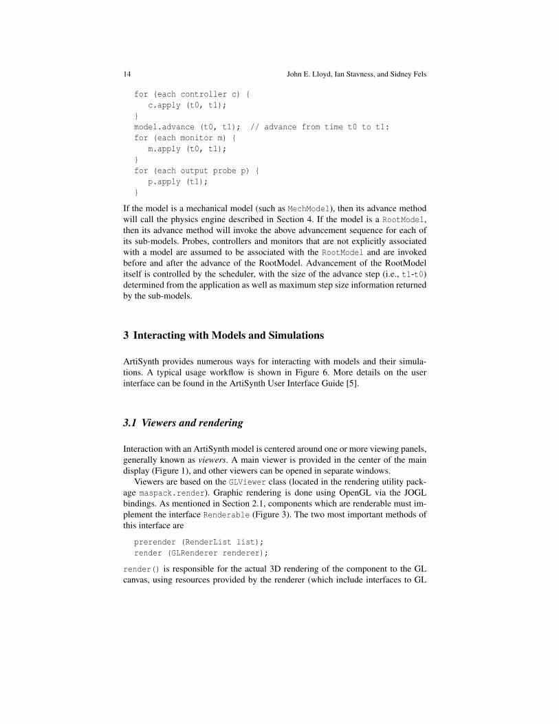
If the model is a mechanical model (such as MechModel), then its advance methodwill call the physics engine described in Section 4. If the model is a RootModel,then its advance method will invoke the above advancement sequence for each ofits sub-models. Probes, controllers and monitors that are not explicitly associatedwith a model are assumed to be associated with the RootModel and are invokedbefore and after the advance of the RootModel. Advancement of the RootModelitself is controlled by the scheduler, with the size of the advance step (i.e., t1-t0)determined from the application as well as maximum step size information returnedby the sub-models.
3 Interacting with Models and Simulations
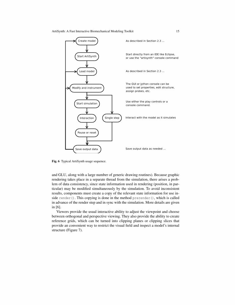
ArtiSynth provides numerous ways for interacting with models and their simula-tions. A typical usage workflow is shown in Figure 6. More details on the userinterface can be found in the ArtiSynth User Interface Guide [5].
3.1 Viewers and rendering
Interaction with an ArtiSynth model is centered around one or more viewing panels,generally known as viewers. A main viewer is provided in the center of the maindisplay (Figure 1), and other viewers can be opened in separate windows.
Viewers are based on the GLViewer class (located in the rendering utility pack-age maspack.render). Graphic rendering is done using OpenGL via the JOGLbindings. As mentioned in Section 2.1, components which are renderable must im-plement the interface Renderable (Figure 3). The two most important methods ofthis interface are
prerender (RenderList list);render (GLRenderer renderer);
render() is responsible for the actual 3D rendering of the component to the GLcanvas, using resources provided by the renderer (which include interfaces to GL
ArtiSynth: A Fast Interactive Biomechanical Modeling Toolkit 15
Fig. 6 Typical ArtiSynth usage sequence.
and GLU, along with a large number of generic drawing routines). Because graphicrendering takes place in a separate thread from the simulation, there arises a prob-lem of data consistency, since state information used in rendering (position, in par-ticular) may be modified simultaneously by the simulation. To avoid inconsistentresults, components must create a copy of the relevant state information for use in-side render(). This copying is done in the method prerender(), which is calledin advance of the render step and in sync with the simulation. More details are givenin [6].
Viewers provide the usual interactive ability to adjust the viewpoint and choosebetween orthogonal and perspective viewing. They also provide the ability to createreference grids, which can be turned into clipping planes or clipping slices thatprovide an convenient way to restrict the visual field and inspect a model’s internalstructure (Figure 7).
16 John E. Lloyd, Ian Stavness, and Sidney Fels
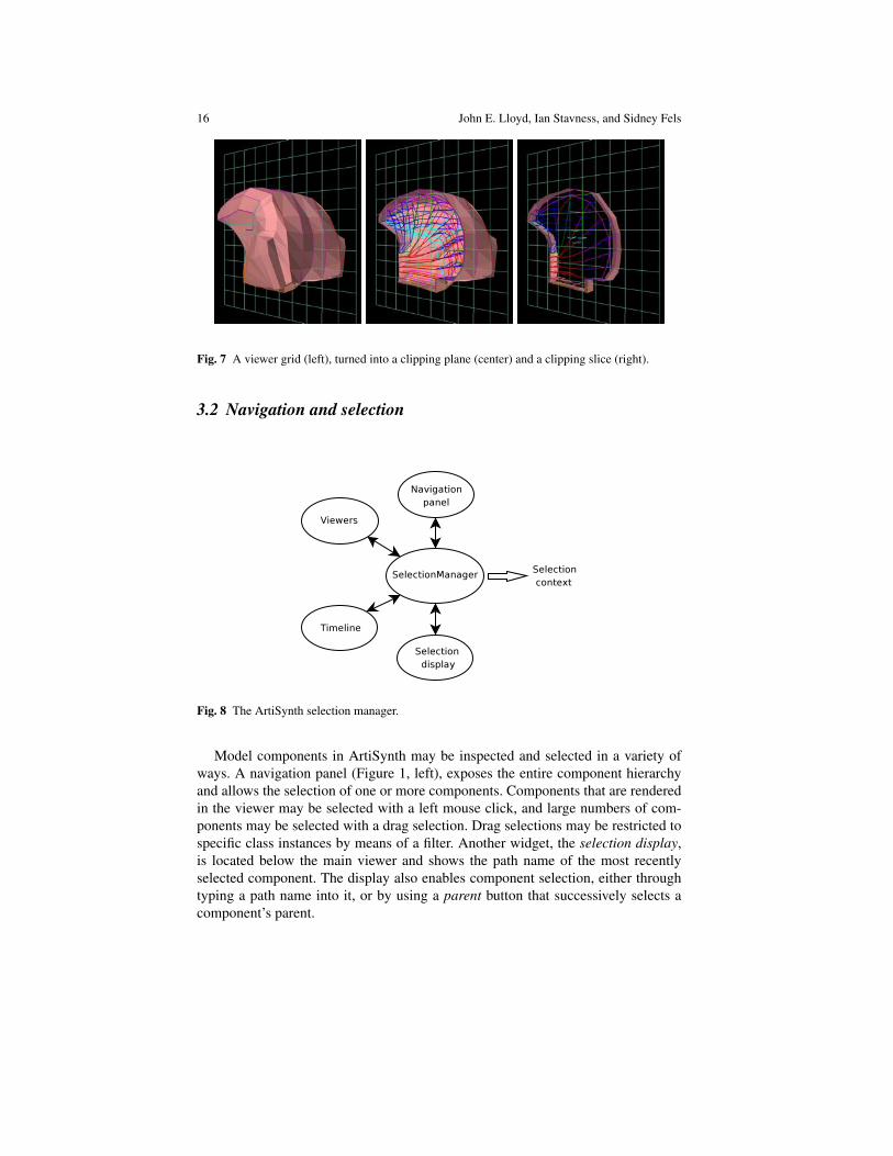
Fig. 7 A viewer grid (left), turned into a clipping plane (center) and a clipping slice (right).
3.2 Navigation and selection
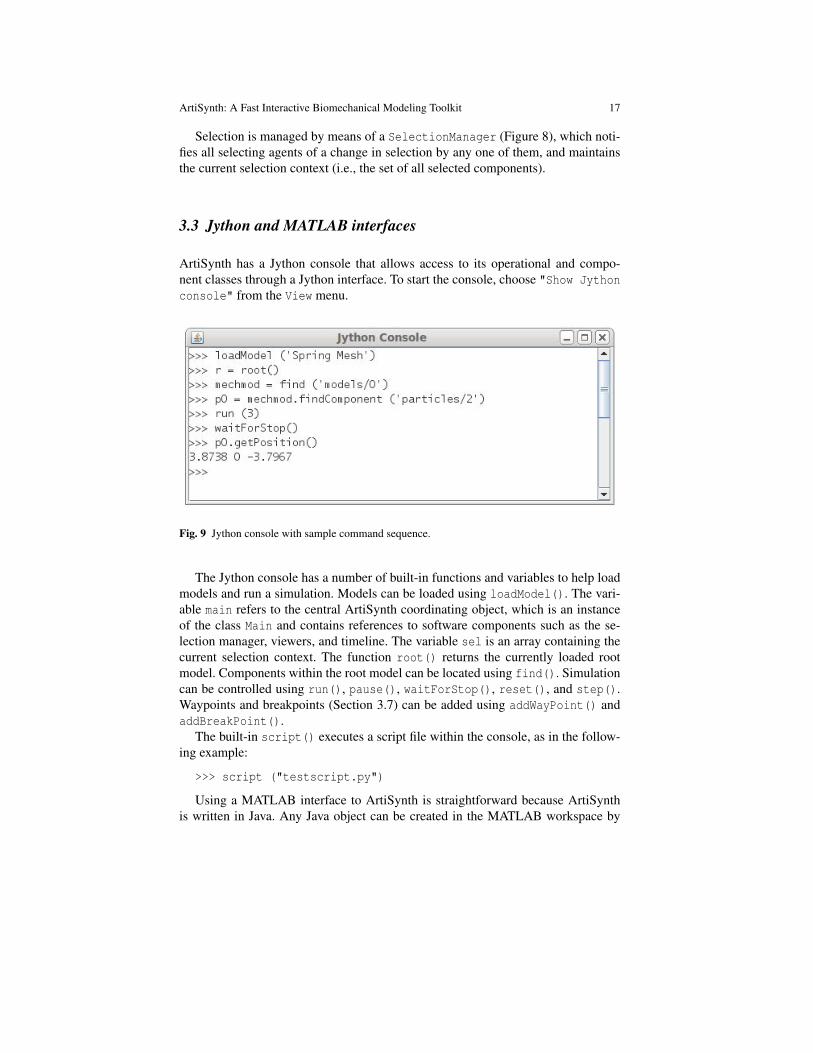
Fig. 8 The ArtiSynth selection manager.
Model components in ArtiSynth may be inspected and selected in a variety ofways. A navigation panel (Figure 1, left), exposes the entire component hierarchyand allows the selection of one or more components. Components that are renderedin the viewer may be selected with a left mouse click, and large numbers of com-ponents may be selected with a drag selection. Drag selections may be restricted tospecific class instances by means of a filter. Another widget, the selection display,is located below the main viewer and shows the path name of the most recentlyselected component. The display also enables component selection, either throughtyping a path name into it, or by using a parent button that successively selects acomponent’s parent.
ArtiSynth: A Fast Interactive Biomechanical Modeling Toolkit 17
Selection is managed by means of a SelectionManager (Figure 8), which noti-fies all selecting agents of a change in selection by any one of them, and maintainsthe current selection context (i.e., the set of all selected components).
3.3 Jython and MATLAB interfaces
ArtiSynth has a Jython console that allows access to its operational and compo-nent classes through a Jython interface. To start the console, choose "Show Jythonconsole" from the View menu.
Fig. 9 Jython console with sample command sequence.
The Jython console has a number of built-in functions and variables to help loadmodels and run a simulation. Models can be loaded using loadModel(). The vari-able main refers to the central ArtiSynth coordinating object, which is an instanceof the class Main and contains references to software components such as the se-lection manager, viewers, and timeline. The variable sel is an array containing thecurrent selection context. The function root() returns the currently loaded rootmodel. Components within the root model can be located using find(). Simulationcan be controlled using run(), pause(), waitForStop(), reset(), and step().Waypoints and breakpoints (Section 3.7) can be added using addWayPoint() andaddBreakPoint().
The built-in script() executes a script file within the console, as in the follow-ing example:
>>> script ("testscript.py")
Using a MATLAB interface to ArtiSynth is straightforward because ArtiSynthis written in Java. Any Java object can be created in the MATLAB workspace by
18 John E. Lloyd, Ian Stavness, and Sidney Fels
calling the constructor for that class1. ArtiSynth can be launched from MATLAB byfirst adding ArtiSynth classes to MATLAB’s classpath. The ArtiSynth Main classcan then be instantiated as follows:
>> main = artisynth.core.driver.Main;
and other ArtiSynth objects can then be accessed through main:
>> main.loadModel(’Spring Mesh’);>> rootmodel = main.getRootModel();
As with the Jython console, the MATLAB interface is a convenient way to scriptmultiple simulations. It is also a powerful way to interface with user defined MAT-LAB scripts and functions for pre-processing input probe data and for plotting andanalyzing output data from simulations.
3.4 Transforming geometry
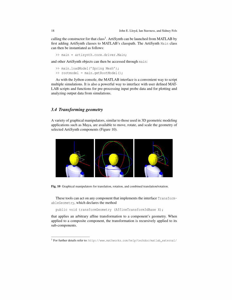
A variety of graphical manipulators, similar to those used in 3D geometric modelingapplications such as Maya, are available to move, rotate, and scale the geometry ofselected ArtiSynth components (Figure 10).
Fig. 10 Graphical manipulators for translation, rotation, and combined translation/rotation.
These tools can act on any component that implements the interface Transform-ableGeometry, which declares the method
public void transformGeometry (AffineTransform3dBase X);
that applies an arbitrary affine transformation to a component’s geometry. Whenapplied to a composite component, the transformation is recursively applied to itssub-components.
1 For further details refer to: http://www.mathworks.com/help/techdoc/matlab_external/
ArtiSynth: A Fast Interactive Biomechanical Modeling Toolkit 19
3.5 Editing properties
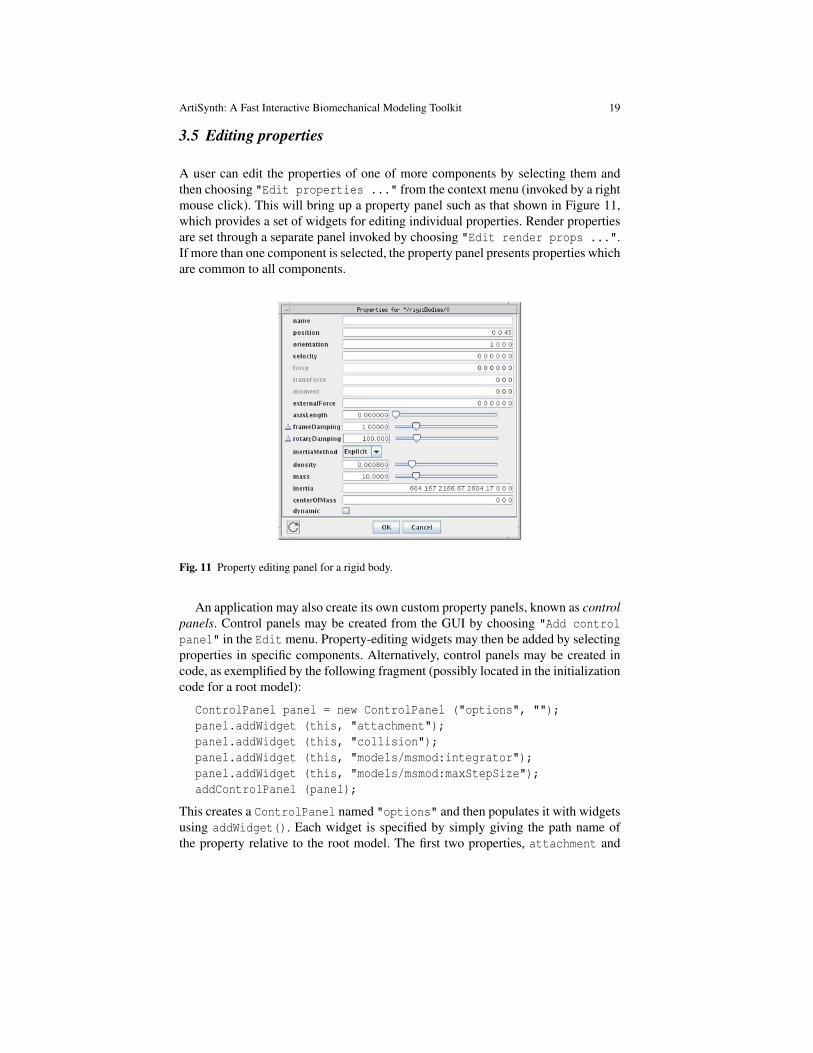
A user can edit the properties of one of more components by selecting them andthen choosing "Edit properties ..." from the context menu (invoked by a rightmouse click). This will bring up a property panel such as that shown in Figure 11,which provides a set of widgets for editing individual properties. Render propertiesare set through a separate panel invoked by choosing "Edit render props ...".If more than one component is selected, the property panel presents properties whichare common to all components.
Fig. 11 Property editing panel for a rigid body.
An application may also create its own custom property panels, known as controlpanels. Control panels may be created from the GUI by choosing "Add controlpanel" in the Edit menu. Property-editing widgets may then be added by selectingproperties in specific components. Alternatively, control panels may be created incode, as exemplified by the following fragment (possibly located in the initializationcode for a root model):
ControlPanel panel = new ControlPanel ("options", "");panel.addWidget (this, "attachment");panel.addWidget (this, "collision");panel.addWidget (this, "models/msmod:integrator");panel.addWidget (this, "models/msmod:maxStepSize");addControlPanel (panel);
This creates a ControlPanel named "options" and then populates it with widgetsusing addWidget(). Each widget is specified by simply giving the path name ofthe property relative to the root model. The first two properties, attachment and
20 John E. Lloyd, Ian Stavness, and Sidney Fels
collision, are properties of the root model itself, while the next two belong todescendant components. The appropriate widgets are created automatically usinginformation about the properties’ type. When finished, the panel is added to the rootmodel using addControlPanel().
A wide variety of widgets for graphically setting different quantities are definedin the package artisynth.core.gui.widgets.
3.6 Structural editing
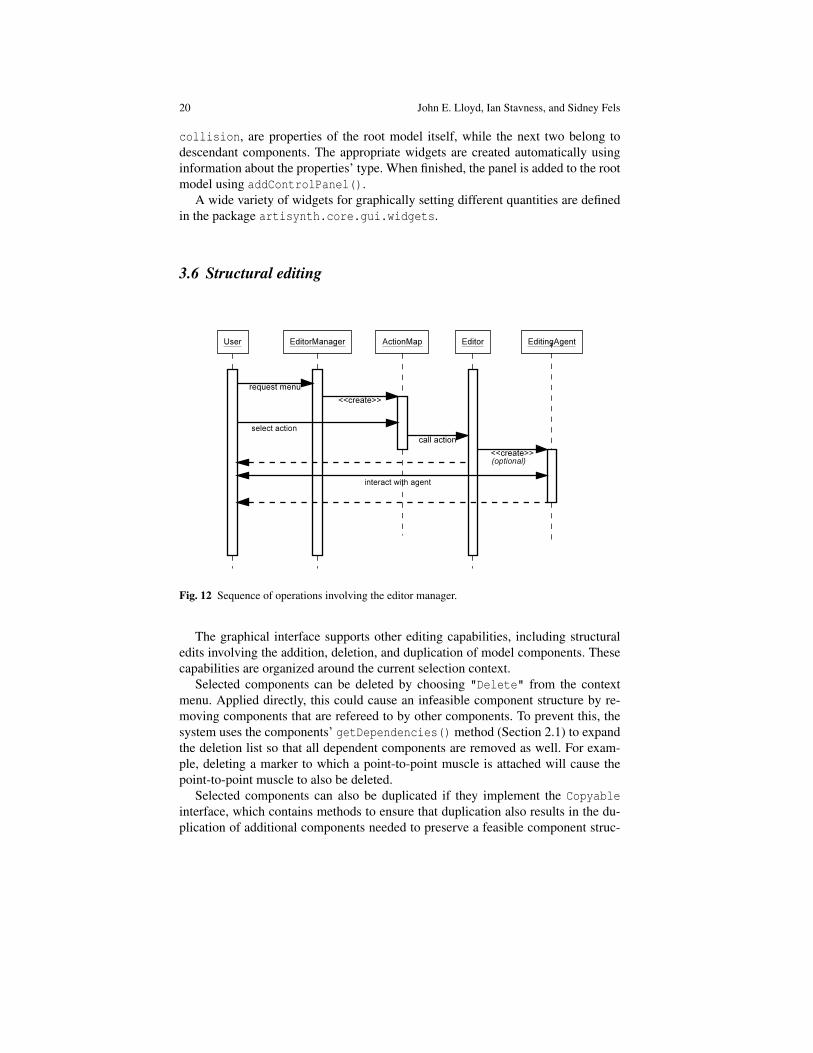
Fig. 12 Sequence of operations involving the editor manager.
The graphical interface supports other editing capabilities, including structuraledits involving the addition, deletion, and duplication of model components. Thesecapabilities are organized around the current selection context.
Selected components can be deleted by choosing "Delete" from the contextmenu. Applied directly, this could cause an infeasible component structure by re-moving components that are refereed to by other components. To prevent this, thesystem uses the components’ getDependencies() method (Section 2.1) to expandthe deletion list so that all dependent components are removed as well. For exam-ple, deleting a marker to which a point-to-point muscle is attached will cause thepoint-to-point muscle to also be deleted.
Selected components can also be duplicated if they implement the Copyableinterface, which contains methods to ensure that duplication also results in the du-plication of additional components needed to preserve a feasible component struc-
ArtiSynth: A Fast Interactive Biomechanical Modeling Toolkit 21
ture. For example, when duplicating a point-to-point muscle the points to which themuscle is attached are also duplicated.
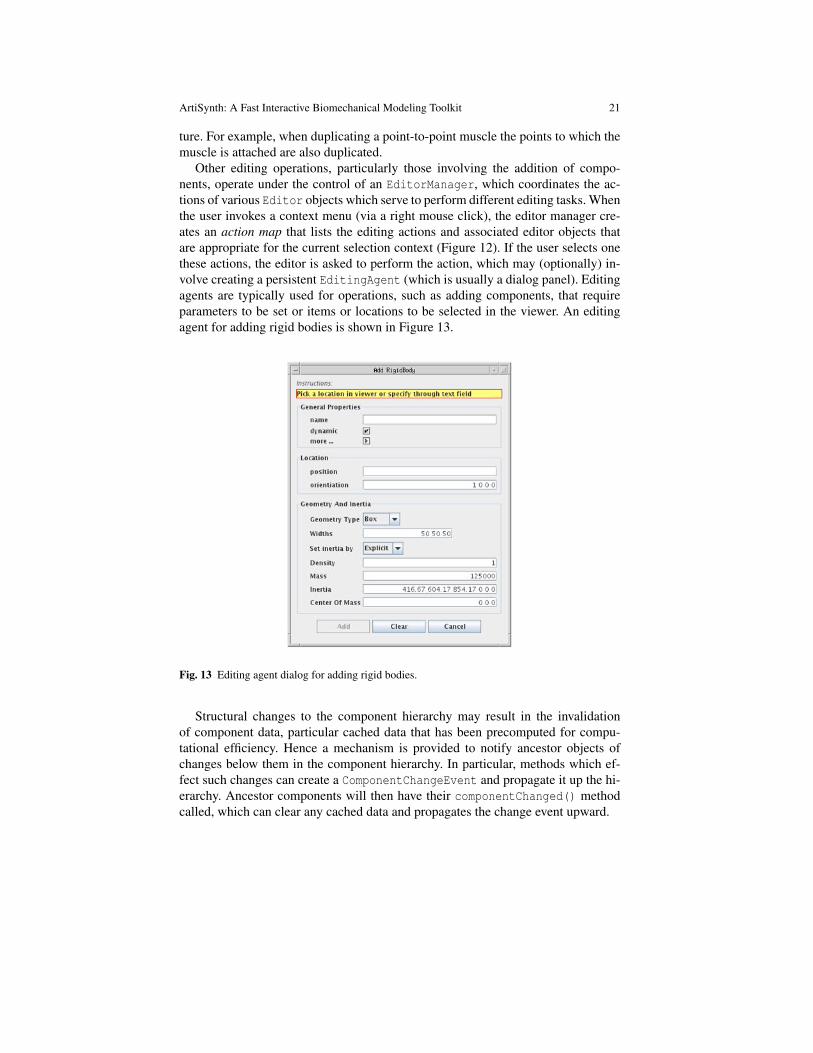
Other editing operations, particularly those involving the addition of compo-nents, operate under the control of an EditorManager, which coordinates the ac-tions of various Editor objects which serve to perform different editing tasks. Whenthe user invokes a context menu (via a right mouse click), the editor manager cre-ates an action map that lists the editing actions and associated editor objects thatare appropriate for the current selection context (Figure 12). If the user selects onethese actions, the editor is asked to perform the action, which may (optionally) in-volve creating a persistent EditingAgent (which is usually a dialog panel). Editingagents are typically used for operations, such as adding components, that requireparameters to be set or items or locations to be selected in the viewer. An editingagent for adding rigid bodies is shown in Figure 13.
Fig. 13 Editing agent dialog for adding rigid bodies.
Structural changes to the component hierarchy may result in the invalidationof component data, particular cached data that has been precomputed for compu-tational efficiency. Hence a mechanism is provided to notify ancestor objects ofchanges below them in the component hierarchy. In particular, methods which ef-fect such changes can create a ComponentChangeEvent and propagate it up the hi-erarchy. Ancestor components will then have their componentChanged() methodcalled, which can clear any cached data and propagates the change event upward.
22 John E. Lloyd, Ian Stavness, and Sidney Fels
3.7 The timeline
Fig. 14 Timeline with probes expanded to show data.
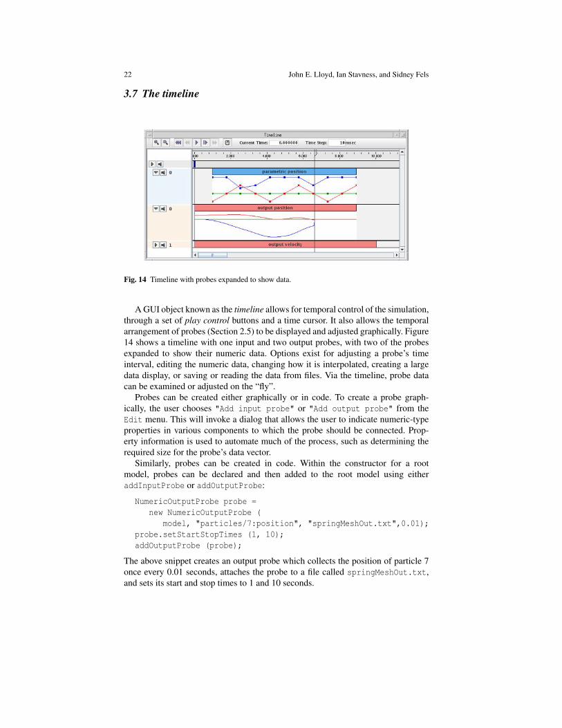
A GUI object known as the timeline allows for temporal control of the simulation,through a set of play control buttons and a time cursor. It also allows the temporalarrangement of probes (Section 2.5) to be displayed and adjusted graphically. Figure14 shows a timeline with one input and two output probes, with two of the probesexpanded to show their numeric data. Options exist for adjusting a probe’s timeinterval, editing the numeric data, changing how it is interpolated, creating a largedata display, or saving or reading the data from files. Via the timeline, probe datacan be examined or adjusted on the “fly”.
Probes can be created either graphically or in code. To create a probe graph-ically, the user chooses "Add input probe" or "Add output probe" from theEdit menu. This will invoke a dialog that allows the user to indicate numeric-typeproperties in various components to which the probe should be connected. Prop-erty information is used to automate much of the process, such as determining therequired size for the probe’s data vector.
Similarly, probes can be created in code. Within the constructor for a rootmodel, probes can be declared and then added to the root model using eitheraddInputProbe or addOutputProbe:
NumericOutputProbe probe =new NumericOutputProbe (
model, "particles/7:position", "springMeshOut.txt",0.01);probe.setStartStopTimes (1, 10);addOutputProbe (probe);
The above snippet creates an output probe which collects the position of particle 7once every 0.01 seconds, attaches the probe to a file called springMeshOut.txt,and sets its start and stop times to 1 and 10 seconds.
ArtiSynth: A Fast Interactive Biomechanical Modeling Toolkit 23
The timeline can also be used to set simulation waypoints and breakpoints. Awaypoint is a time location where state is saved when the simulation passes throughit, enabling the system to reset itself to that time later using the play control buttons(one cannot normally set the system to an arbitrary time since this requires physicalsimulation from a known state). A number of uniformly spaced waypoints can beused to create an animation of the simulation. A breakpoint is simply a waypoint atwhich simulation is also halted.
4 Physical Simulation
Physical simulation is required to advance ArtiSynth models forward in time. Inparticular, the advance method for the top-most mechanical model in the hierarchyneeds to solve the second-order ordinary differential equation (ODE) that resultsfrom the physics of the mechanical system. How that is done is the focus of thissection. Much of the material is taken from [37].
As mentioned in Section 2.2, ArtiSynth components can be roughly divided intodynamic components, force effectors, and constraints. At present, there are only twotypes of dynamic component: a six DOF RigidBody, and a three DOF Particle(the nodes of finite element models are subclasses of Particle). Other types ofdynamic components, such as reduced coordinate FEM models, may be added inthe future.
4.1 The mechanical system ODE
In this section we present the ODE associated with the mechanical system2. Let qand u be the generalized positions and velocities of all the dynamical componentsin the model hierarchy, with q related to u by q = Qu (Q generally equals theidentity, except for components such as rigid bodies, where it maps angular velocityonto the derivative of a unit quaternion). Let f(q ,u , t) be the force produced by allthe force effector components (including the finite elements), and let M be the com-posite mass matrix. For FEM models we currently use a lumped mass model, whichensures that M is block diagonal and makes it easier to interconnect FEMs withmass-spring and rigid body components. By representing rigid body velocity andacceleration in body coordinates we can also ensure that M is constant. Newton’ssecond law then gives
Mu = f(q ,u , t). (1)
In addition, bilateral and unilateral constraints give rise to locally linear constraintson u of the form
2 Since the ODE contains algebraic constraints, it is technically a differential algebraic equation,or DAE.
24 John E. Lloyd, Ian Stavness, and Sidney Fels
G(q)u = 0, N(q)u � 0. (2)
Bilateral constraints include rigid body joints, FEM incompressibility associatedwith the mixed u-P formulation [20], and point-surface constraints, while unilateralconstraints include contact and joint limits. Constraints give rise to constraint forces(in the directions G(q)T and N(q)T ) which supplement the forces of (1) in orderto enforce the constraint conditions. In addition, for unilateral constraints, we havea complementarity condition in which Nu > 0 implies no constraint force, and aconstraint force implies Nu = 0. Any given constraint usually involves only a fewdynamic components and so G and N are generally sparse.
4.2 Solving the ODE by trapezoidal integration
Solving the equations of motion requires integrating (1) together with (2). ArtiSynthprovides a number of integrators, both explicit and implicit, for doing this. Whendeformable bodies are present, the mechanical system is usually stiff, implying theneed for an implicit integrator to obtain efficient performance. One of the morecommonly used implicit integrators supplied by ArtiSynth is a semi-implicit second-order Newmark integrator [23], with g = 1/2 and b = 1/4, known more generallyas the trapezoidal rule.
Letting k denote the index of values at a particular time step, and h denote thetime step size, this leads to the update rules
u k+1 = u k +h2(u k + u k+1), q k+1 = q k +
h2(Q ku k +Q k+1u k+1), (3)
subject toG k+1u k+1 = 0, N k+1u k+1 � 0. (4)
Since G and N tend to vary slowly between time steps we can approximate (4)using
G ku k+1 = g k, N ku k+1 � n k, (5)
where g k ⌘ �hG ku k and n k ⌘ �hN ku k. Likewise, we use the approximationQ k+1 ⇡ Q k + hQ k. For u k+1, recalling that M is constant, an estimate of the (un-constrained) value of u k+1 can be obtained from u k+1 ⇡ M�1f k+1, with f k+1 ap-proximated by the first-order Taylor series
f k+1 ⇡ f k +∂f k
∂uDu +
∂f k
∂qDq .
Placing this into the expression for u k+1 in (3), multiplying by M , noting that
Dq = h/2(Q ku k +Q k+1u k+1) and Du = u k+1 �u k,
ArtiSynth: A Fast Interactive Biomechanical Modeling Toolkit 25
and incorporating the constraints (5), we obtain the mixed linear complementarityproblem
0
B@M k �G kT �N kT
G k 0 0N k 0 0
1
CA
0
@u k+1
l
l
l
z
1
A+
0
@�Mu k �hf k
�g k
�n k
1
A=
0
@00w
1
A ,
0 z ? w � 0, (6)
where w is a slack variable, l
l
l and z give the average constraint impulses over thetime step, and
M k ⌘ M � h2
∂f k
∂u� h2
4∂f k
∂qQ k+1 and f k ⌘ f k � 1
2∂f k
∂uu k +
h4
∂f k
∂qQ ku k.
The complementarity condition for unilateral constraints is enforced by 0 z ?w � 0. A more detailed explanation of this formulation can be found in [27].
A single solve of (6) is required to determine u k+1 for each semi-implicit inte-gration step. A fully implicit integrator (not currently implemented in ArtiSynth)would require (6) to be applied iteratively at each time step.
It should be noted that other integration schemes can result in same system as(6), only with different values for M k and f k. For example, for the first order semi-implicit Euler scheme, we have
M k ⌘ M �h∂f k
∂u�h2 ∂f k
∂qQ k+1 and f k ⌘ f k �h
∂f k
∂uu k,
while for the explicit forward Euler scheme we have M k ⌘ M and f k ⌘ f k.For finite element models, the localized stiffness and damping matrices are em-
bedded within ∂f k/∂q and ∂f k/∂u , which means that for models dominated by FEMcomponents M will have an FEM sparsity structure.
4.3 Friction, damping, and stabilization
Coulomb (dry) friction can be added to system (6) by including extra constraints thatcreate frictional forces along directions tangent to the contact points. A linearizedfriction cone [4, 27] can be created that provides an arbitrarily accurate frictionapproximation (depending on the number of facets in the cone), but results in a sys-tem of equations that is no longer positive-semidefinite and must be solved usingtechniques such as Lemke’s algorithm [13] which are difficult to implement in a nu-merically robust way. Box friction [21] is a more approximate model that assumesthe magnitudes of the contact normal forces are known a-priori (typically from theprevious solve step), but adds at most two extra constraints per contact point to (6)and can be solved using relatively robust pivoting methods such as Keller’s algo-
26 John E. Lloyd, Ian Stavness, and Sidney Fels
rithm [21]. Since Coulomb friction effects in our models tend to be small, ArtiSynthcurrently implements the numerically simpler box friction, applying it as a post-hoccorrection to u k+1 (in a manner similar to [30]), using a simplified version of (6),with M instead of M .
Different forms of viscous damping are available, including translational and ro-tary damping applied directly to particles and rigid bodies, and damping terms em-bedded in point-to-point springs and muscle actuators. For FEM models, Rayleighdamping is available, which takes the form
D F = aM F +bK F ,
where M F is the portion of the (lumped) mass matrix associated with the FEMnodes and K F is the (instantaneous) FEM stiffness matrix. D F is then embeddedwithin the overall system matrix ∂f/∂u .
In addition to solving for velocities, it is also necessary to correct positions to ac-count for drift from the constraints, including interpenetrations arising from contact.This can be done at each time step using a modified form of (6) which computes animpulse dq that corrects the positions while honoring the constraints:
0
B@M k �G kT �N kT
G k 0 0N k 0 0
1
CA
0
@dql
l
l
z
1
A+
0
@0d
d
dgd
d
dn
1
A=
0
@00w
1
A ,
0 z ? w � 0, (7)
where d
d
dg and d
d
dn are the constraint displacements that must be corrected. If thecorrections are sufficiently small, it is often permissible to use M in place of M k,which improves solution efficiency since M is constant and block-diagonal.
While such stabilization can sometimes be incorporated directly into (6) [3], weprefer to perform the position correction separately as this (a) allows for the possibil-ity of an iterative correction in the case of larger errors, and (b) explicitly separatesthe computed velocities from the impulses used to correct errors.
4.4 System solution and complexity
For notational convenience, in this section we will drop the k superscripts from M ,G , N , g , n , and f in (6) and assume that these quantities are all evaluated at timestep k.
System (6) is a large, sparse mixed linear complementarity problem [13] that isnot particularly easy to solve, given the unilateral constraints and the fact that Mis not block diagonal. If M is symmetric positive definite (SPD), it is equivalent toa convex quadratic program. If there are no unilateral constraints (N = /
0), then itreduces to a linear Karush-Kuhn-Tucker (KKT) system.
ArtiSynth: A Fast Interactive Biomechanical Modeling Toolkit 27
Generally, M is symmetric (unsymmetric terms sometimes arise from rotationaleffects but these are usually small enough to ignore) and hence will also be SPD forsmall enough h (since M is SPD). However, the resulting system is still harder tosolve than non-stiff multibody systems where M = M . This is because M , whilestill sparse, is not block-diagonal. Multibody systems are often solved using the pro-jected Gauss-Seidel method [21]. However, this involves a sequence of iterations,each requiring the computation of G iM
�1G Ti or N iM
�1N Ti , which is easy to do
for a block-diagonal M but much more costly for M .At present, ArtiSynth solves (6) by using a Schur complement to turn it into a
dense regular linear complementarity problem
NA�1N T z + NA�1b �n = w0 z ? w � 0 (8)
where
A ⌘✓
M �G T
G 0
◆, N ⌘
�N 0
�, b ⌘
✓Mu k +hf
g
◆.
which is solved using Keller’s algorithm [21]. u k+1 and l
l
l can then be obtainedusing back-substitution:
✓u k+1
l
l
l
◆= A�1
⇣b + N T z
⌘. (9)
Keller’s algorithm is a pivoting method with an expected complexity of O(m3),where m is the number of unilateral constraints. In addition, forming (8) and back-solving (9) requires m+ 1 solves of a system involving A . This is done using thePardiso sparse direct solver [28], and entails a once-per-step factoring of A , plusm+1 solve operations. Experimentally, we have determined that the complexity offactoring A (using Pardiso) for 3D FEM type problems is roughly O(n1.7), where nis the size of A . Similarly, we have also determined that the complexity of solvinga factored A is roughly O(n1.3). Hence we can expect the overall complexity forsolving (6) to be
O(m3)+mO(n1.3)+O(n1.7).
This works well provided that the number of unilateral constraints m is small. Tohelp achieve this, we can sometimes treat the unilateral constraints arising fromcontact as bilateral constraints (i.e., entries in G ) on a per-step basis, as describedfurther in Section 4.7.
4.5 Attachments between bodies
In creating comprehensive anatomical models, it is often necessary to attach variousbodies together. Most typically, this is done by connecting points of one body to
28 John E. Lloyd, Ian Stavness, and Sidney Fels
REST UNATTACHED
FEM ATTACHEDFEM & BLOCK ATTACHED
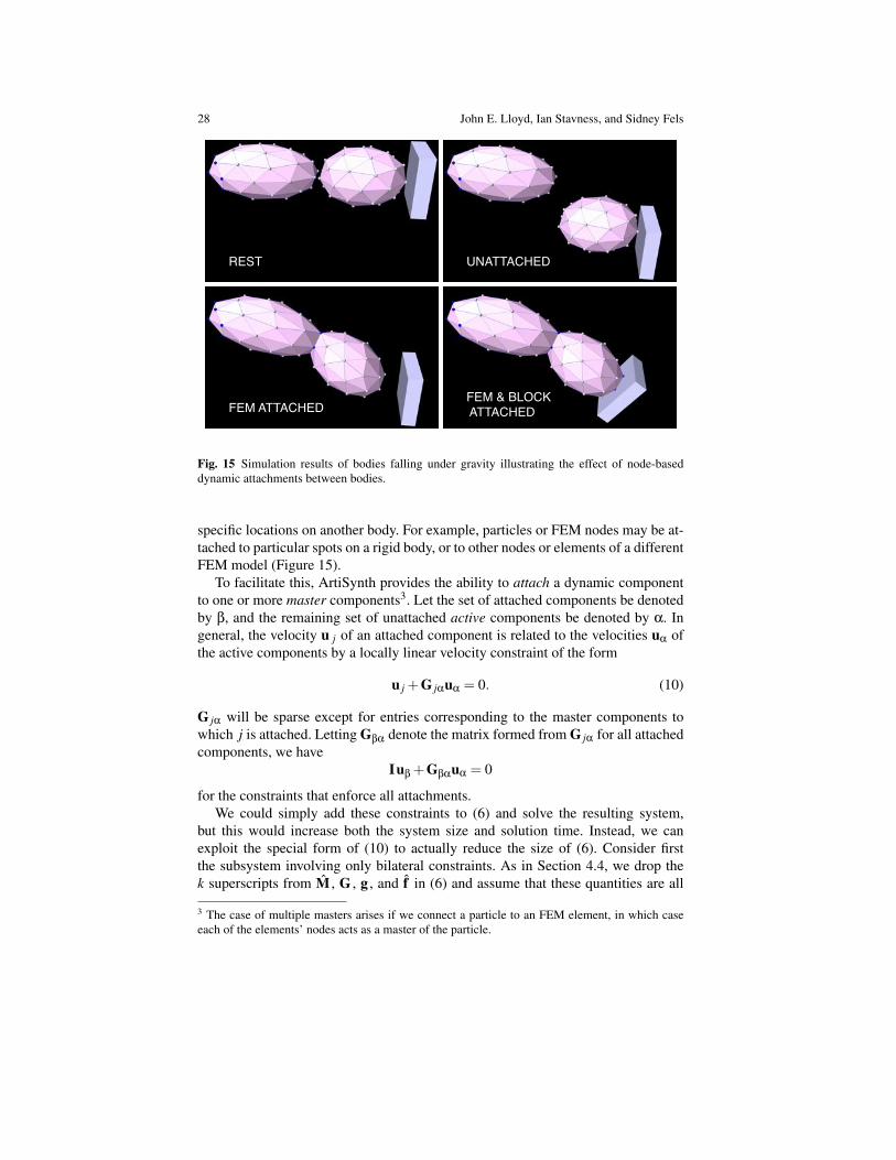
Fig. 15 Simulation results of bodies falling under gravity illustrating the effect of node-baseddynamic attachments between bodies.
specific locations on another body. For example, particles or FEM nodes may be at-tached to particular spots on a rigid body, or to other nodes or elements of a differentFEM model (Figure 15).
To facilitate this, ArtiSynth provides the ability to attach a dynamic componentto one or more master components3. Let the set of attached components be denotedby b, and the remaining set of unattached active components be denoted by a. Ingeneral, the velocity u j of an attached component is related to the velocities u
a
ofthe active components by a locally linear velocity constraint of the form
u j +G jaua
= 0. (10)
G ja will be sparse except for entries corresponding to the master components towhich j is attached. Letting G
ba
denote the matrix formed from G ja for all attachedcomponents, we have
Iub
+Gba
ua
= 0
for the constraints that enforce all attachments.We could simply add these constraints to (6) and solve the resulting system,
but this would increase both the system size and solution time. Instead, we canexploit the special form of (10) to actually reduce the size of (6). Consider firstthe subsystem involving only bilateral constraints. As in Section 4.4, we drop thek superscripts from M , G , g , and f in (6) and assume that these quantities are all
3 The case of multiple masters arises if we connect a particle to an FEM element, in which caseeach of the elements’ nodes acts as a master of the particle.
ArtiSynth: A Fast Interactive Biomechanical Modeling Toolkit 29
evaluated at time step k. Letting b ⌘ Mu k + hf and partitioning the system intoactive and attached components yields
0
BB@
Maa
Mab
GTaa
GTba
Mba
Mbb
GTab
IG
aa
Gab
0 0G
ba
I 0 0
1
CCA
0
BB@
uk+1a
uk+1b
l
l
l
a
l
l
l
b
1
CCA=
0
BB@
ba
bb
ga
0
1
CCA .
The identity submatrices make it easy to solve for uk+1b
and l
l
l
b
:
uk+1b
=�Gba
uk+1a
, l
l
l
b
= bb
�Mba
uk+1a
+Mbb
Gba
uk+1a
�GTab
l
l
l
a
and hence reduce the system to✓
M 0 G 0T
G 0 0
◆✓uk+1
a
l
l
l
a
◆=
✓b 0
ga
◆(11)
where
M 0 ⌘ PMP T , G 0 ⌘ GP T , b 0 ⌘ Pb , with P ⌘⇣
I �GTba
⌘.
Similarly, unilateral constraints can be reduced via N 0 = NP T . The reductionoperation can be performed in O(n) time and results in a system that is less sparsebut generally faster to solve than the original.
4.6 Kinematic control
It is possible to control selected dynamic components kinematically, so that theirvelocities are explicitly specified by an external source (such as a probe). The forcesacting on kinematically controlled components then become the unknowns that aresolved for. This is useful in situations where certain parts of a system’s movementare known a priori and we wish to determine the response of the rest of the system.In particular, it provides an easy way to include experimentally recorded kinematicdata in a simulation. A dynamic component can be made kinematic by setting itsdynamic property to false.
The solution for a system containing kinematic components is arranged as fol-lows. Let the set of active components be denoted by a, and the let the kinematiccomponents be r. As in Section 4.5, we consider first only bilateral constraints, andpartition (6) between a and r to obtain:
0
@M
aa
Mar
GTa
Mra
Mrr
GTr
Ga
Gr
0
1
A
0
@v
a
vr
l
l
l
1
A=
0
@fa
fr
g
g
g
1
A .
30 John E. Lloyd, Ian Stavness, and Sidney Fels
Since vr
is given, we can reduce the system to✓
Maa
GTa
Ga
0
◆✓v
a
l
l
l
◆=
✓fa
�Mar
vr
g
g
g�Gr
vr
◆.
and then solve for fr
as
fr
= Mra
va
+Mrr
vr
+GTr
l
l
l
A similar reduction can be applied to unilateral constraints, and an analogous,though more complex, formulation works in the presence of attachments.
4.7 Contact handling
t = 0s t = 0.25s t = 0.5s
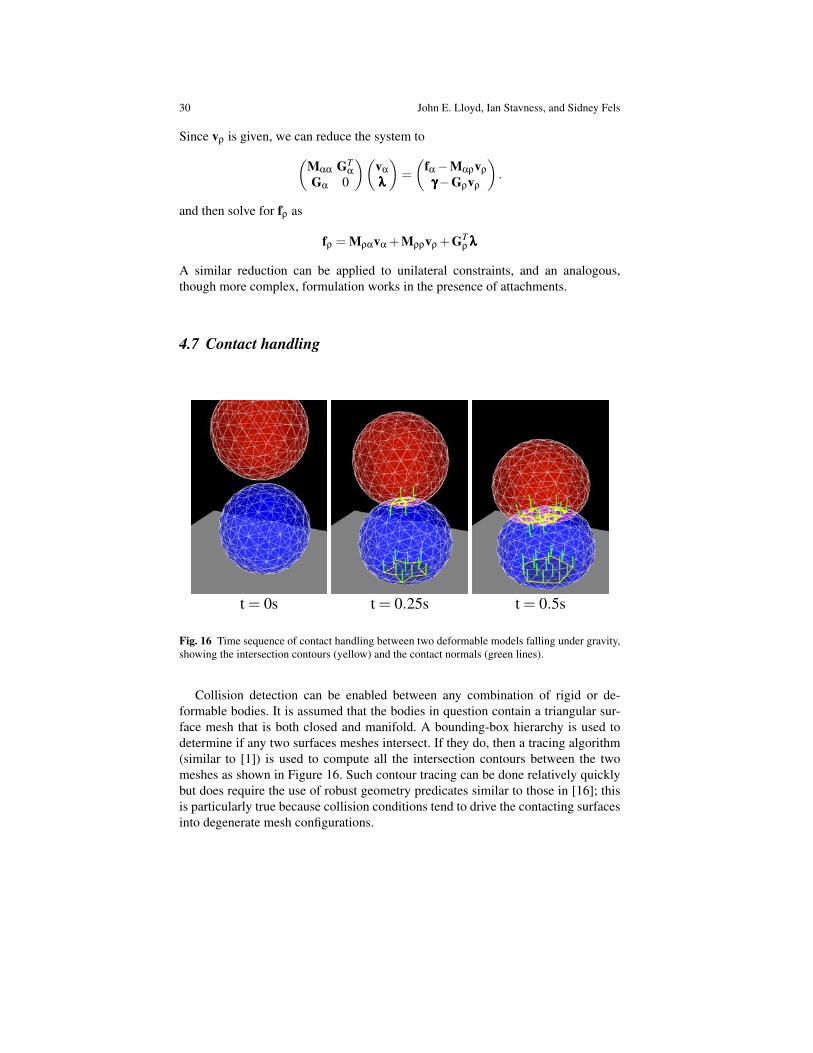
Fig. 16 Time sequence of contact handling between two deformable models falling under gravity,showing the intersection contours (yellow) and the contact normals (green lines).
Collision detection can be enabled between any combination of rigid or de-formable bodies. It is assumed that the bodies in question contain a triangular sur-face mesh that is both closed and manifold. A bounding-box hierarchy is used todetermine if any two surfaces meshes intersect. If they do, then a tracing algorithm(similar to [1]) is used to compute all the intersection contours between the twomeshes as shown in Figure 16. Such contour tracing can be done relatively quicklybut does require the use of robust geometry predicates similar to those in [16]; thisis particularly true because collision conditions tend to drive the contacting surfacesinto degenerate mesh configurations.
ArtiSynth: A Fast Interactive Biomechanical Modeling Toolkit 31
Determining the intersection contour allows us to create a set of constraints forcorrecting the interpenetration and preventing interpenetrating velocities. For rigidbodies, this is done by fitting a plane to each contour, projecting the contour ontothis plane, and then sampling the vertices of the projection’s 2D convex hull tocreate individual contact points, using the planar normal as the contact normal. Fordeformable bodies, contact constraints are generated for each interpenetrating nodeas described in [37]. The intersection contour can also provide an estimate of thecontact area, which can be used for determining contact pressure.
As mentioned in Section 4.4, the solution time of (6) can be greatly improved ifsome contact constraints can be temporarily treated as bilateral constraints withina particular time step. By default, ArtiSynth does this for contact involving de-formable bodies, since such bodies have many degrees of freedom and their con-tact constraints tend to be somewhat decoupled. To prevent sticking, each contact’svertex-face pair is stored between time steps, and if it reappears in the next step, itis used as a contact constraint only if its corresponding l
l
l value computed in (6) is� 0, implying that there is no force trying to make it separate. This is effectively anactive set method, with the active set used to solve (6) being updated between steps.
4.8 Physics engine summary
The ArtiSynth physics engine, using the trapezoidal integrator, is summarized be-low. It is applicable to most second-order mechanical systems which use a La-grangian representation of component state. For other ArtiSynth integrators, thestructure is similar.
1. Compute contacts (as per Section 4.7) and the bilateral and unilateral con-straint matrices G k and N k.
2. Correct positions q k to remove interpenetration and drift errors, using (7).3. If necessary, adjust G k and N k to reflect changes in q .4. Solve for u k+1 using (6).5. Adjust velocities u k+1 for dry friction, as described in Section 4.3.6. Compute new positions: q k+1 = q k +h/2(Q k+1u k+1 +Q ku k).
4.9 Interfacing the physics engine to ArtiSynth
The physics engine is implemented by the class MechSystemSolver, which is in-voked by the advance method of mechanical models (Section 2.5) to advance them-selves forward in time.
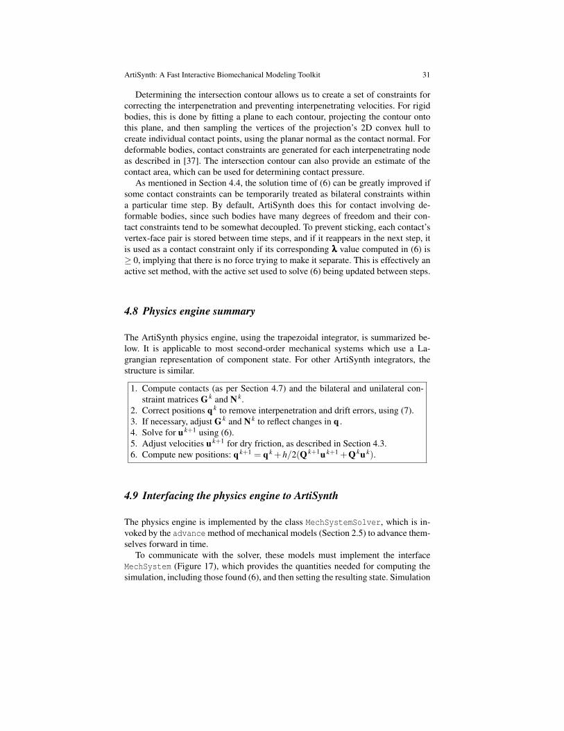
To communicate with the solver, these models must implement the interfaceMechSystem (Figure 17), which provides the quantities needed for computing thesimulation, including those found (6), and then setting the resulting state. Simulation
32 John E. Lloyd, Ian Stavness, and Sidney Fels
quantities include state, mass, forces, force Jacobians, and constraint information.The MechSystem interface provides a clean separation between the physics simu-lation and the ArtiSynth component structure, allowing the possibility for new anddifferent simulation mechanisms to be used in the future.
Fig. 17 ArtiSynth mechanical models, such as MechModel and the basic FEM model FemModel,must implement MechSystem, shown partially here.
5 Inverse simulation
ArtiSynth provides inverse simulation capabilities that compute muscle activationsrequired for a forward-dynamics model to track a prescribed kinematic task. This isa useful feature as it is often difficult to reliably measure muscle activations experi-mentally, or to estimate activations by hand for a particular model. In our trajectory-tracking formulation, muscle activations are determined using a quadratic programthat minimizes the errors for a desired movement goal while resolving motor re-dundancy at each integration time step. The description here is based on material in[31], Chapter 4.
For inverse simulation, the mechanical system forces are divided into passive andactive components, so that
f = f p(q ,u , t)+ f a(q ,u ,a(t))
ArtiSynth: A Fast Interactive Biomechanical Modeling Toolkit 33
where q and u are the position and velocity state vectors and a is a vector of muscleactivation levels (bounded between 0 and 1). We assume that f a is locally linear withrespect to a (which is true for a standard Hill-type muscle model), so that
f a = L(q ,u)a ,
where L is a matrix.At present, inverse simulation in ArtiSynth is currently only supported for sys-
tems with bilateral constraints4. The velocities u k+1 and constraint impulses l
l
l canbe determined from (6), which reduces to a linear system since we are not consider-ing unilateral constraints:
M k �G kT
G k 0
!✓u k+1
l
l
l
◆=
Mu k +hf k
+hL
kag k
!. (12)
We wish to determine a at the beginning of each forward-dynamics integrationtime step so as to track a movement goal. The movement goal is specified by a targetvelocity v ⇤ in a target velocity space v that is related to the system velocities u viaa Jacobian matrix J m, so that v = J mu . For time step k+ 1, it is easy to see from(12) that u k+1 is linear with respect to a , so that
u k+1 = u 0 +H ua ,
where u 0 is the solution of u k+1 for (12) with a set to zero, and each column j ofH u is the solution of u k+1 for (12) with a right hand side of
✓L
ke j0
◆, e j ⌘ elementary unit vector. (13)
We minimize the velocity tracking error kv ⇤ �J mu k+1k, which can be expressed inquadratic form as
fm(a)⌘12kv �H mak2, (14)
withv ⌘ v ⇤ �J mu 0 and H m ⌘ J mH u.
For some applications, such as computing muscle activations to generate a pre-scribed bite force with a dynamic jaw model (as done in [33]), we may also wishto specify a constraint force target x
x
x that is related to the constraint impulses l
l
l viaa Jacobian matrix, J c, so that hx
x
x = J cl
l
l. We minimize the constraint force trackingerror khx
x
x�J cl
l
lk, which can be expressed as
fc(a)⌘12kl
l
l�H cak2, (15)
4 The addition of unilateral constraints leads to a more complex mathematical programming prob-lem with complementarity constraints (MPCC).
34 John E. Lloyd, Ian Stavness, and Sidney Fels
withl
l
l ⌘ hx
x
x�J ml
l
l0 and H c ⌘ J cHl
,
where l
l
l0 and Hl
are computed in a similar manner as described for u 0 and H u.To resolve activation redundancies, we also include a weighted l2�norm regu-
larization term, 12 a T Wa , where W is a diagonal weighting matrix.
Combining the movement and constraint force goals, regularization, and muscleactivations bounds, we arrive at the following quadratic program:
mina
wmfm(a)+wcfc(a)+wa
2a T W�1a
subject to 0 a 1, (16)
where wm, wc, and wa are weights used to trade off between cost terms. This for-mulation can be extended to include optimizations over other biologically relevantvariables, such as stiffness or metabolic energy.
The optimization program (16) is solved at the beginning of each time step, usinga special built-in Controller (Section 2.5), in order to determine the activations tobe used in the forward dynamics simulation. The ArtiSynth system solver is usedto compute v , H m, l
l
l, and H c. The resulting quadratic program is dense but tendsto be small since its dimension is the size of a , i.e. the number of activations beingsolved for. The quadratic program is also convex, which means it can be solved as alinear complementarity problem, which is done using the ArtiSynth implementationof Keller’s algorithm [21].
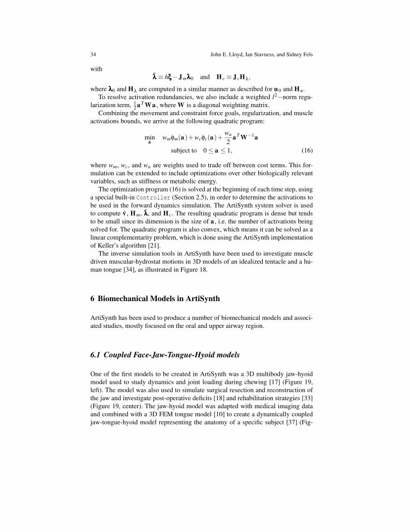
The inverse simulation tools in ArtiSynth have been used to investigate muscledriven muscular-hydrostat motions in 3D models of an idealized tentacle and a hu-man tongue [34], as illustrated in Figure 18.
6 Biomechanical Models in ArtiSynth
ArtiSynth has been used to produce a number of biomechanical models and associ-ated studies, mostly focused on the oral and upper airway region.
6.1 Coupled Face-Jaw-Tongue-Hyoid models
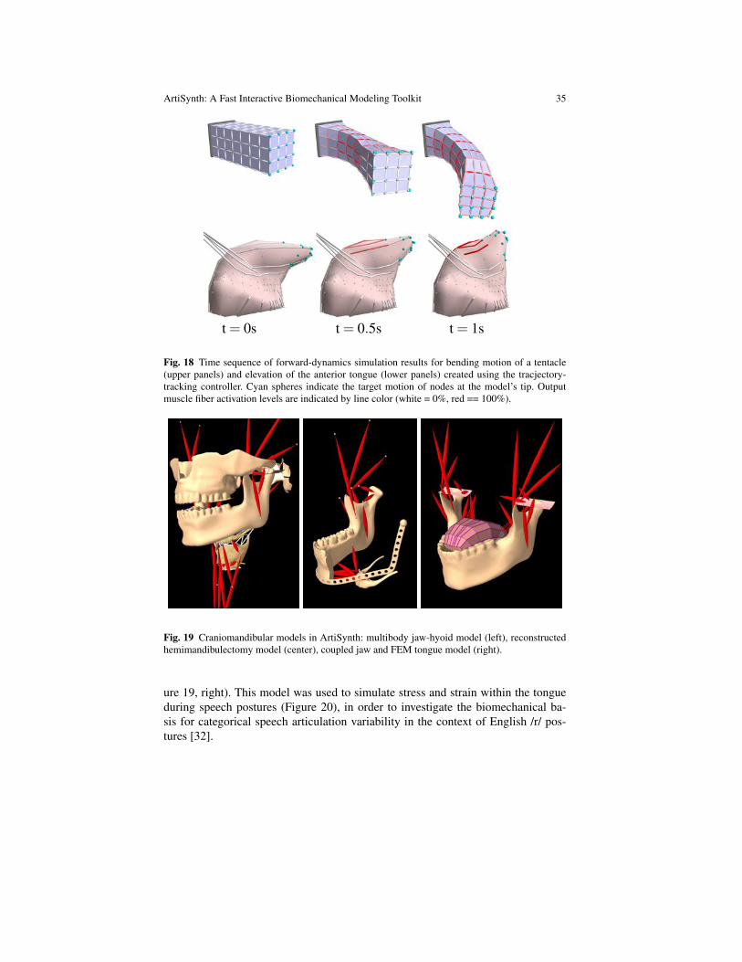
One of the first models to be created in ArtiSynth was a 3D multibody jaw-hyoidmodel used to study dynamics and joint loading during chewing [17] (Figure 19,left). The model was also used to simulate surgical resection and reconstruction ofthe jaw and investigate post-operative deficits [18] and rehabilitation strategies [33](Figure 19, center). The jaw-hyoid model was adapted with medical imaging dataand combined with a 3D FEM tongue model [10] to create a dynamically coupledjaw-tongue-hyoid model representing the anatomy of a specific subject [37] (Fig-
ArtiSynth: A Fast Interactive Biomechanical Modeling Toolkit 35
t = 0s t = 0.5s t = 1s
Fig. 18 Time sequence of forward-dynamics simulation results for bending motion of a tentacle(upper panels) and elevation of the anterior tongue (lower panels) created using the tracjectory-tracking controller. Cyan spheres indicate the target motion of nodes at the model’s tip. Outputmuscle fiber activation levels are indicated by line color (white = 0%, red == 100%).
Fig. 19 Craniomandibular models in ArtiSynth: multibody jaw-hyoid model (left), reconstructedhemimandibulectomy model (center), coupled jaw and FEM tongue model (right).
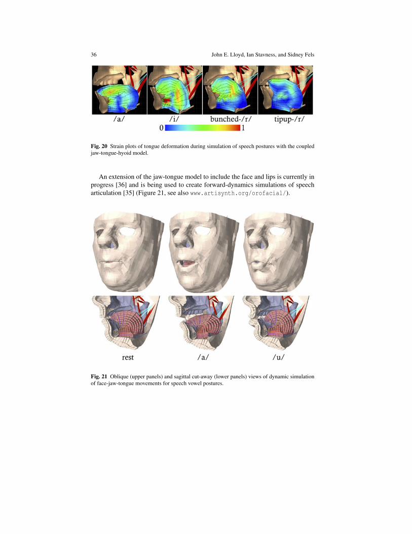
ure 19, right). This model was used to simulate stress and strain within the tongueduring speech postures (Figure 20), in order to investigate the biomechanical ba-sis for categorical speech articulation variability in the context of English /r/ pos-tures [32].
36 John E. Lloyd, Ian Stavness, and Sidney Fels
Fig. 20 Strain plots of tongue deformation during simulation of speech postures with the coupledjaw-tongue-hyoid model.
An extension of the jaw-tongue model to include the face and lips is currently inprogress [36] and is being used to create forward-dynamics simulations of speecharticulation [35] (Figure 21, see also www.artisynth.org/orofacial/).
Fig. 21 Oblique (upper panels) and sagittal cut-away (lower panels) views of dynamic simulationof face-jaw-tongue movements for speech vowel postures.
ArtiSynth: A Fast Interactive Biomechanical Modeling Toolkit 37
6.2 Comprehensive upper airway model
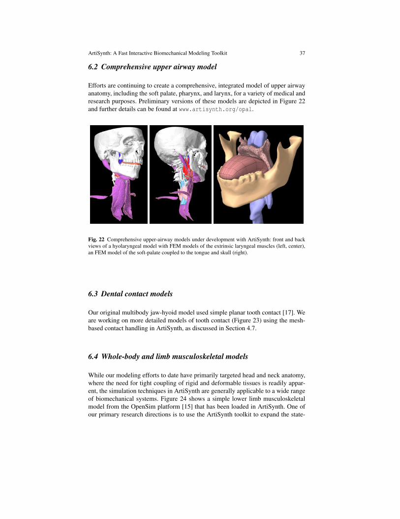
Efforts are continuing to create a comprehensive, integrated model of upper airwayanatomy, including the soft palate, pharynx, and larynx, for a variety of medical andresearch purposes. Preliminary versions of these models are depicted in Figure 22and further details can be found at www.artisynth.org/opal.
Fig. 22 Comprehensive upper-airway models under development with ArtiSynth: front and backviews of a hyolaryngeal model with FEM models of the extrinsic laryngeal muscles (left, center),an FEM model of the soft-palate coupled to the tongue and skull (right).
6.3 Dental contact models
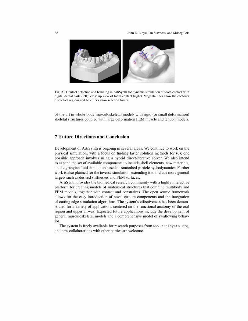
Our original multibody jaw-hyoid model used simple planar tooth contact [17]. Weare working on more detailed models of tooth contact (Figure 23) using the mesh-based contact handling in ArtiSynth, as discussed in Section 4.7.
6.4 Whole-body and limb musculoskeletal models
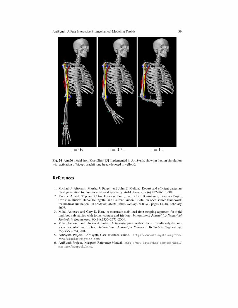
While our modeling efforts to date have primarily targeted head and neck anatomy,where the need for tight coupling of rigid and deformable tissues is readily appar-ent, the simulation techniques in ArtiSynth are generally applicable to a wide rangeof biomechanical systems. Figure 24 shows a simple lower limb musculoskeletalmodel from the OpenSim platform [15] that has been loaded in ArtiSynth. One ofour primary research directions is to use the ArtiSynth toolkit to expand the state-
38 John E. Lloyd, Ian Stavness, and Sidney Fels
Fig. 23 Contact detection and handling in ArtiSynth for dynamic simulation of tooth contact withdigital dental casts (left); close up view of tooth contact (right). Magenta lines show the contoursof contact regions and blue lines show reaction forces.
of-the-art in whole-body musculoskeletal models with rigid (or small deformation)skeletal structures coupled with large deformation FEM muscle and tendon models.
7 Future Directions and Conclusion
Development of ArtiSynth is ongoing in several areas. We continue to work on thephysical simulation, with a focus on finding faster solution methods for (6); onepossible approach involves using a hybrid direct-iterative solver. We also intendto expand the set of available components to include shell elements, new materials,and Lagrangian fluid simulation based on smoothed particle hydrodynamics. Furtherwork is also planned for the inverse simulation, extending it to include more generaltargets such as desired stiffnesses and FEM surfaces.
ArtiSynth provides the biomedical research community with a highly interactiveplatform for creating models of anatomical structures that combine multibody andFEM models, together with contact and constraints. The open source frameworkallows for the easy introduction of novel custom components and the integrationof cutting edge simulation algorithms. The system’s effectiveness has been demon-strated for a variety of applications centered on the functional anatomy of the oralregion and upper airway. Expected future applications include the development ofgeneral musculoskeletal models and a comprehensive model of swallowing behav-ior.
The system is freely available for research purposes from www.artisynth.org,and new collaborations with other parties are welcome.
ArtiSynth: A Fast Interactive Biomechanical Modeling Toolkit 39
t = 0s t = 0.5s t = 1s
Fig. 24 Arm26 model from OpenSim [15] implemented in ArtiSynth, showing flexion simulationwith activation of biceps brachii long head (denoted in yellow).
References
1. Michael J. Aftosmis, Marsha J. Berger, and John E. Melton. Robust and efficient cartesianmesh generation for component-based geometry. AIAA Journal, 36(6):952–960, 1998.
2. Jeremie Allard, Stephane Cotin, Francois Faure, Pierre-Jean Bensoussan, Francois Poyer,Christian Duriez, Herve Delingette, and Laurent Grisoni. Sofa an open source frameworkfor medical simulation. In Medicine Meets Virtual Reality (MMVR), pages 13–18, February2007.
3. Mihai Anitescu and Gary D. Hart. A constraint-stabilized time-stepping approach for rigidmultibody dynamics with joints, contact and friction. International Journal for NumericalMethods in Engineering, 60(14):2335–2371, 2004.
4. Mihai Anitescu and Florian A. Potra. A time-stepping method for stiff multibody dynam-ics with contact and friction. International Journal for Numerical Methods in Engineering,55(7):753–784, 2002.
5. ArtiSynth Project. Artisynth User Interface Guide. http://www.artisynth.org/doc/html/uiguide/uiguide.html.
6. ArtiSynth Project. Maspack Reference Manual. http://www.artisynth.org/doc/html/maspack/maspack.html.
40 John E. Lloyd, Ian Stavness, and Sidney Fels
7. Ted Belytschko, Wing Kam Liu, and Brian Moran. Nonlinear Finite Elements for Continuaand Structures. Wiley, 2000.
8. Javier Bonet and Richard D Wood. Nonlinear Continuum Mechanics for Finite Element Anal-ysis. Cambridge University Press, 2008.
9. Stephanie Buchaillard, Muriel Brix, Pascal Perrier, and Yohan Payan. Simulations of theconsequences of tongue surgery on tongue mobility: Implications for speech production inpost-surgery conditions. International Journal of Medical Robotics and Computer AssistedSurgery, 3(3):252, 2007.
10. Stephanie Buchaillard, Pascal Perrier, and Yohan Payan. A biomechanical model of cardinalvowel production: Muscle activations and the impact of gravity on tongue positioning. Journalof the Acoustical Society of America, 126(4):2033–2051, 2009.
11. Murat Cenk Cavusoglu, Tolga Goktekin, and Frank Tendick. Gipsi: A framework for opensource/open architecture software development for organ-level surgical simulation. IEEETransactions on Information Technology in Biomedicine, 10(2):312–322, 2006.
12. Matthieu Chabanas, Vincent Luboz, and Yohan Payan. Patient specific finite element modelof the face soft tissues for computer-assisted maxillofacial surgery. Medical Image Analysis,7(2):131–151, 2003.
13. Richard W. Cottle, Jong-Shi Pang, and Richard E. Stone. The Linear Complementarity Prob-lem. Academic Press, 1992.
14. Douglas Crockford. The application/json media type for javascript object notation (json).2006.
15. Scott Delp, Frank Anderson, Allison Arnold, Peter Loan, Ayman Habib, Chand John, EranGuendelman, and Darryl Thelen. OpenSim: Open-source software to create and ana-lyze dynamic simulations of movement. IEEE Transactions on Biomedical Engineering,54(11):1940–1950, 2007.
16. Herbert Edelsbrunner and Ernst Peter Mucke. Simulation of simplicity: a technique to copewith degenerate cases in geometric algorithms. ACM Trans. Graph., 9(1):66–104, 1990.
17. Alan G. Hannam, Ian Stavness, John E. Lloyd, and Sidney Fels. A dynamic model of jaw andhyoid biomechanics during chewing. J Biomechanics, 41(5):1069–1076, 2008.
18. Alan G. Hannam, Ian Stavness, John E. Lloyd, Sidney Fels, Art Miller, and Don Curtis. Acomparison of simulated jaw dynamics in models of segmental mandibular resection versusresection with alloplastic reconstruction. Journal of Prosthetic Dentistry, 104(3):191–198,2010.
19. Yaqi Huang, David White, and Atul Malhotra. Use of computational modeling to predictresponses to upper airway surgery in obstructive sleep apnea. Laryngoscope, 117:648–653,2007.
20. Thomas J.R. Hughes. The finite element method: linear static and dynamic finite elementanalysis. Dover Publications, New York, 2000.
21. Claude Lacoursiere. Ghosts and machines: regularized variational methods for interactivesimulations of multibodies with dry frictional contacts. PhD thesis, Computer Science Dept.,Umea University, Sweden, 2007.
22. Donna S. Lundy, Christine Smith, Laura Colangelo, Paula A. Sullivan, Jerilyn A. Logemann,Cathy L. Lazarus, Lisa A. Newman, Tom Murry, Lori Lombard, and Joy Gaziano. Aspiration:cause and implications. Otolaryngology-Head and Neck Surgery, 120(4):474–478, 1999.
23. Christoph Lunk and Benrd Simeon. Solving constrained mechanical systems by the fam-ily of newmark and a-methods. Journal of Applied Mathematics and Mechanics (ZAMM),86(10):772–784, 2006.
24. Kevin Montgomery, Cynthia Bruyns, Joel Brown, Stephen Sorkin, Frederic Mazzella, Guil-laume Thonier, Arnaud Tellier, Benjamin Lerman, and Anil Menon. Spring: A general frame-work for collaborative, real-time surgical simulation. In Medicine Meets Virtual Reality(MMVR), pages 23–26, 2002.
25. Matthias Muller and Markus Gross. Interactive virtual materials. In GI ’04: Proceedings ofGraphics Interface, pages 239–246, 2004.
26. Musculoskeletal Research Laboratories. FEBio: finite elements for biomechanics. http://mrl.sci.utah.edu/software/febio.
ArtiSynth: A Fast Interactive Biomechanical Modeling Toolkit 41
27. Florian A. Potra, Mihai Anitescu, Bogdan Gavrea, and Jeff Trinkle. A linearly implicit trape-zoidal method for integrating stiff multibody dynamics with contact, joints, and friction. In-ternational Journal for Numerical Methods in Engineering, 66(7):1079–1124, 2006.
28. Olaf Schenk and Klaus Gartner. Solving unsymmetric sparse systems of linear equations withPARDISO. Future Gener. Comput. Syst., 20(3):475–487, 2004.
29. Ahmed A. Shabana. Dynamics of Multibody Systems. Cambridge University Press, 1998.30. Tamar Shinar, Craig Schroeder, and Ron Fedkiw. Two-way coupling of rigid and deformable
bodies. In SCA ’08: Proceedings of the 2008 ACM SIGGRAPH/Eurographics Symposium onComputer Animation, pages 95–103, 2008.
31. Ian Stavness. Byte your tongue : a computational model of human mandibular-lingual biome-chanics for biomedical applications. PhD thesis, University of British Columbia, Dept. ofElectrical and Computer Engineering, 2010.
32. Ian Stavness, Bryan Gick, Donald Derrick, and Sidney Fels. Biomechanical modeling ofEnglish /r/ variants. In International Seminar of Speech Production, 2011.
33. Ian Stavness, Alan Hannam, John E. Lloyd, and Sidney Fels. Predicting muscle patterns forhemimandibulectomy models. Computer Methods in Biomechanics & Biomedical Engineer-ing, 13(4):483–491, 2010.
34. Ian Stavness, John Lloyd, and Sidney Fels. Inverse-dynamics simulation of muscular-hydrostat finite-element models. In 23rd International Society of Biomechanics Congress(ISB), number 933, July 2011.
35. Ian Stavness, John Lloyd, Yohan Payan, and Sidney Fels. Towards speech articulation sim-ulation with a dynamic coupled face-jaw-tongue model. In International Seminar of SpeechProduction, 2011.
36. Ian Stavness, John E. Lloyd, Yohan Payan, and Sidney Fels. Dynamic hard-soft tissue modelsfor orofacial biomechanics. In ACM SIGGRAPH Talks, page 1, 2010.
37. Ian Stavness, John E. Lloyd, Yohan Payan, and Sidney Fels. Coupled hard-soft tissue simula-tion with contact and constraints applied to jaw-tongue-hyoid dynamics. International Journalof Numerical Methods in Biomedical Engineering, 27:367–390, 2011.