arX

iv:h

ep-t

h/99

0914

0v2

12

Oct

199

9

hep-th/9909140

ETH-TH/99-25

ESI-759

September 1999

CONFORMAL BOUNDARY CONDITIONS

AND THREE-DIMENSIONAL

TOPOLOGICAL FIELD THEORY

Giovanni Felder , Jurg Frohlich , Jurgen Fuchs and Christoph Schweigert

ETH Zurich

CH – 8093 Zurich

Abstract

We present a general construction of all correlation functions of a two-dimensionalrational conformal field theory, for an arbitrary number of bulk and boundary fieldsand arbitrary topologies. The correlators are expressed in terms of Wilson graphsin a certain three-manifold, the connecting manifold. The amplitudes constructedthis way can be shown to be modular invariant and to obey the correct factorizationrules.

1

Two-dimensional conformal field theory plays a fundamental role in the theory of two-dimensional critical systems of classical statistical mechanics [1], in quasi one-dimensional con-densed matter physics [2] and in string theory [3]. The study of defects in systems of condensedmatter physics [4], of percolation probabilities [5] and of (open) string perturbation theoryin the background of certain string solitons, the so-called D-branes [6], forces one to analyzeconformal field theories on surfaces that may have boundaries and / or can be non-orientable.

In this letter we present a new description of correlation functions of an arbitrary numberof bulk and boundary fields on general surfaces. We also show how to compute various typesof operator product coefficients from our formulas. For simplicity, in this letter we restrictour attention to boundary conditions that preserve all bulk symmetries. Moreover, we takethe modular invariant torus partition function that encodes the spectrum of bulk fields of thetheory to be given by charge conjugation. Technical details and complete proofs will appear ina separate publication.

Given a chiral conformal field theory, such as a chiral free boson, our aim is to computecorrelation functions on a two-dimensional surface X that may be non-orientable and can havea boundary. To this end, we first construct the so-called double X of the surface X . Thisis an oriented surface, on which an orientation reversing map σ of order two acts in such away that X is obtained as the quotient of X by σ. Thus X is a two-fold cover of X ; but thiscover is branched over the boundary points, which correspond to fixed points of the map σ.For example, when X is the disk D, then X is the two-sphere and σ is the reflection aboutits equatorial plane. For X the cross-cap, i.e. the real projective plane RP

2, X is again thetwo-sphere, but σ is now the antipodal map. Finally, when X is closed and orientable, thedouble X consists of two disconnected copies of X with opposite orientation, X ∼=X⊔(−X).

Quite generally, correlation functions on a surface X can be constructed from conformalblocks on its double X [7,8]. As a first step, one has to find the pre-images on X of all insertionpoints on X , and associate a primary field of the chiral conformal field theory to each of them.Since bulk points have two pre-images, for a bulk field two chiral labels j and j∗ are needed,corresponding to left and right movers. Boundary fields, in contrast, carry a single label k; yet,they should not be thought of as chiral objects.

Having associated these labels to the geometric data, we can assign a vector space of confor-mal blocks, not necessarily of dimension one, to every collection of bulk and boundary fields onX . The correlation function is one specific element in this space. This element must obey mod-ular invariance and factorization properties. The conformal bootstrap programme [3] allows todetermine the correlation function by imposing these properties as constraints. Fortunately,the connection between conformal field theory in two dimensions and topological field theoryin three dimensions supplies us with a most direct way to construct concrete elements in thespaces of conformal blocks. What one must do in order to specify a a definite element in thespace of conformal blocks is to find a three-manifold MX whose boundary is X ,

∂MX = X , (1)

as well as a Wilson graph W in MX that ends at the marked points on X. This can be done forany arbitrary rational conformal field theory; for details, which are based on the axiomatizationin [9], we refer to [10]. In the particular case of WZW models, Chern--Simons theory can beused [11, 12, 13] for this construction. For these models, the element in the space of conformal

2

blocks is obtained by the Chern--Simons path integral∫

DA W exp ( i k

4π

∫

MX

Tr (A∧dA + 23 A∧A∧A) ) (2)

with appropriate parabolic conditions at the punctures.

Thus to obtain a correlation function on X , we first construct a certain three-manifold MX

with boundary X , which we call the connecting three-manifold . Technically, the manifold MX

can be characterized as follows. When X does not have a boundary, thenMX = (X×[−1,1])/Z2,where the group Z2 acts on X by σ and on the interval [−1,1] by the sign flip t 7→−t fort∈ [−1,1]. Thus MX consists of pairs (x, t) with x a point on the double X and t in [−1,1],modulo the identification (x, t)∼ (σ(x),−t). For fixed x, the points of the form (x, t) form asegment, the connecting interval , joining the two pre-images of a point in X . When X has aboundary, we obtainMX from (X × [−1,1])/Z2 by contracting the connecting intervals over theboundary to single points, in such a way that MX remains a smooth manifold. (An equivalentconstruction, in which the boundary intervals are not contracted, was given in [13].)

It is readily checked that the boundary of the connecting manifold MX is indeed the doubleX . Moreover, MX connects the two pre-images of a bulk point by an interval in such a mannerthat the connecting intervals for distinct bulk points do not intersect. Let us list a few examples.For a disk, the connecting manifold is a solid three-ball, and the connecting intervals are allperpendicular to the equatorial plane. Similarly, when X is the annulus, MX is a solid torus.For X the cross-cap, the connecting manifold MX is best characterized by the fact that whenglueing to its boundary a solid ball, we obtain S3/Z2

∼=RP3, which coincides with the group

manifold of the Lie group SO(3). For closed orientable surfaces X , the bundle MX is just thetrivial bundle X × [−1,1]; e.g. when X is a sphere, then MX can be visualized as consisting ofthe points between two concentric spheres.

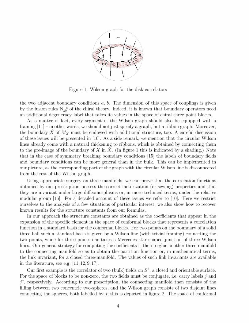
The next step is to specify a certain Wilson graph in MX . The prescription, which isillustrated in figure 1 for the case of a disk with an arbitrary number of insertions in the bulkand on the boundary, is as follows. First, for every bulk insertion j, one joins the pre-images ofthe insertion point by a Wilson line running along the connecting interval. Next, one inserts onecircular Wilson line parallel to each component of the boundary (a similar idea was presentedin [13]) and joins every boundary insertion k on the respective boundary component by a shortWilson line to the corresponding circular Wilson line. Moreover, the circular Wilson lines arerequired to run “close to the boundary”, in the sense that none of the connecting intervals ofthe bulk fields passes between the circular Wilson lines and the boundary of X .

So far we have only specified the geometric information for the conformal blocks. To proceed,we also must attach a primary label of the chiral conformal field theory to each segment of theWilson graph. For the bulk points, this prescription is immediate, as we are dealing with thecharge conjugation modular invariant. Similarly, we are naturally provided with the labels k forthe short Wilson lines that connect the boundary insertions with the circular Wilson lines. Inaddition, the segments of the circular Wilson lines should encode the boundary conditions of thecorresponding boundary segments. Recalling that those boundary conditions which preserve allbulk symmetries can be labelled by the primary fields of the chiral conformal field theory [14],we attach such a primary label a to every segment of the circular Wilson lines. Finally, we mustconsider the three-valent junctions on the circular Wilson lines. For each of them we choosean element α in the space of chiral couplings between the label k for the boundary field and

3

������������������������������������������������������������������������������������������

������������������������������������������������������������������������������������������

������������������������������������������������������

������������������������������������������������������

������������������������������������������

������������������������������������������

������������������������������������

������������������������������������

���������������

���������������

�����������������������������������������������������������������������������

�����������������������������������������������������������������������������

����������������������������������������

����������������������������������������

�����������������������������������

�����������������������������������

���������������������

���������������������

��������������������������������������������������������

��������������������������������������������������������

��������������������������������������������������������

��������������������������������������������������������

�����������������������������������

�����������������������������������

...

...

Figure 1: Wilson graph for the disk correlators

the two adjacent boundary conditions a, b. The dimension of this space of couplings is givenby the fusion rules N a

kb of the chiral theory. Indeed, it is known that boundary operators needan additional degeneracy label that takes its values in the space of chiral three-point blocks.

As a matter of fact, every segment of the Wilson graph should also be equipped with aframing [11] – in other words, we should not just specify a graph, but a ribbon graph. Moreover,the boundary X of MX must be endowed with additional structure, too. A careful discussionof these issues will be presented in [10]. As a side remark, we mention that the circular Wilsonlines already come with a natural thickening to ribbons, which is obtained by connecting themto the pre-image of the boundary of X in X . (In figure 1 this is indicated by a shading.) Notethat in the case of symmetry breaking boundary conditions [15] the labels of boundary fieldsand boundary conditions can be more general than in the bulk. This can be implemented inour picture, as the corresponding part of the graph with the circular Wilson line is disconnectedfrom the rest of the Wilson graph.

Using appropriate surgery on three-manifolds, we can prove that the correlation functionsobtained by our prescription possess the correct factorization (or sewing) properties and thatthey are invariant under large diffeomorphisms or, in more technical terms, under the relativemodular group [16]. For a detailed account of these issues we refer to [10]. Here we restrictourselves to the analysis of a few situations of particular interest; we also show how to recoverknown results for the structure constants from our formulas.

In our approach the structure constants are obtained as the coefficients that appear in theexpansion of the specific element in the space of conformal blocks that represents a correlationfunction in a standard basis for the conformal blocks. For two points on the boundary of a solidthree-ball such a standard basis is given by a Wilson line (with trivial framing) connecting thetwo points, while for three points one takes a Mercedes star shaped junction of three Wilsonlines. Our general strategy for computing the coefficients is then to glue another three-manifoldto the connecting manifold so as to obtain the partition function or, in mathematical terms,the link invariant, for a closed three-manifold. The values of such link invariants are availablein the literature, see e.g. [11, 12, 9, 17].

Our first example is the correlator of two (bulk) fields on S2, a closed and orientable surface.For the space of blocks to be non-zero, the two fields must be conjugate, i.e. carry labels j andj∗, respectively. According to our prescription, the connecting manifold then consists of thefilling between two concentric two-spheres, and the Wilson graph consists of two disjoint linesconnecting the spheres, both labelled by j; this is depicted in figure 2. The space of conformal

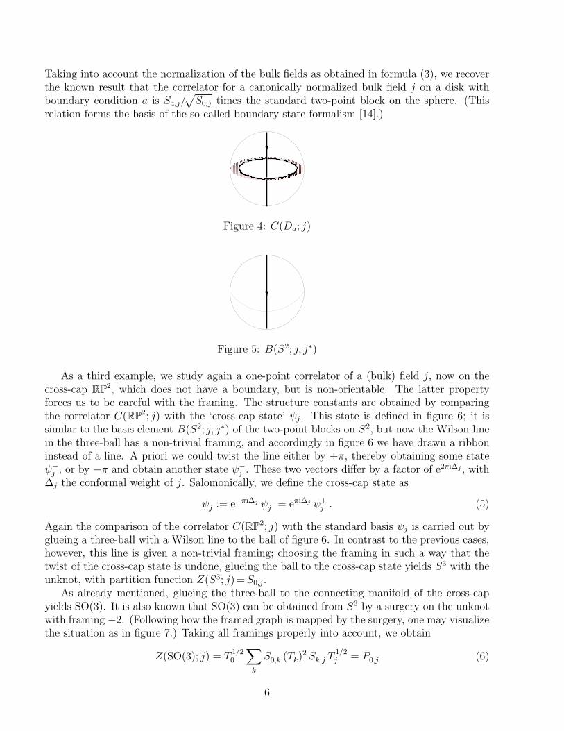
4

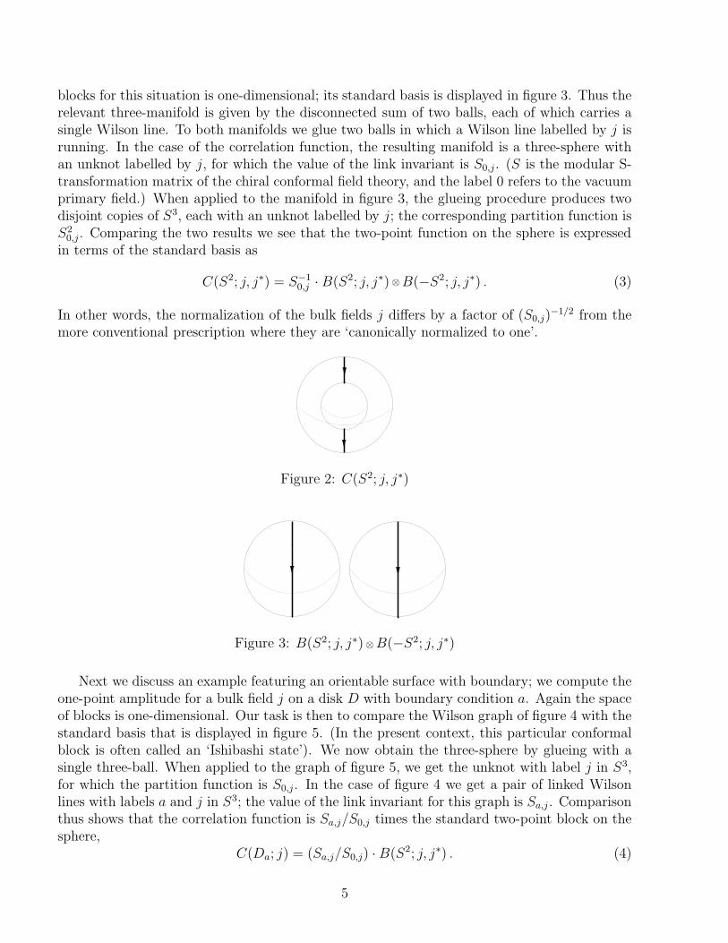
blocks for this situation is one-dimensional; its standard basis is displayed in figure 3. Thus therelevant three-manifold is given by the disconnected sum of two balls, each of which carries asingle Wilson line. To both manifolds we glue two balls in which a Wilson line labelled by j isrunning. In the case of the correlation function, the resulting manifold is a three-sphere withan unknot labelled by j, for which the value of the link invariant is S0,j. (S is the modular S-transformation matrix of the chiral conformal field theory, and the label 0 refers to the vacuumprimary field.) When applied to the manifold in figure 3, the glueing procedure produces twodisjoint copies of S3, each with an unknot labelled by j; the corresponding partition function isS20,j . Comparing the two results we see that the two-point function on the sphere is expressed

in terms of the standard basis as

C(S2; j, j∗) = S−10,j · B(S2; j, j∗) ⊗B(−S2; j, j∗) . (3)

In other words, the normalization of the bulk fields j differs by a factor of (S0,j)−1/2 from the

more conventional prescription where they are ‘canonically normalized to one’.

Figure 2: C(S2; j, j∗)

Figure 3: B(S2; j, j∗) ⊗B(−S2; j, j∗)

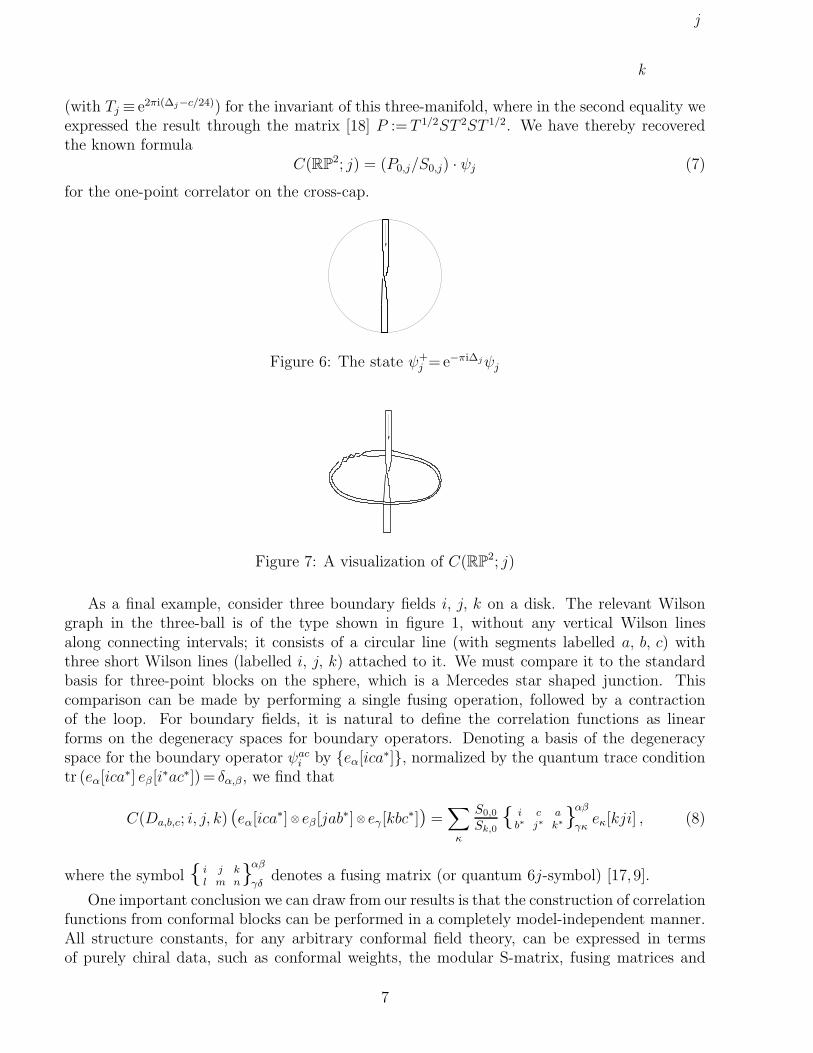
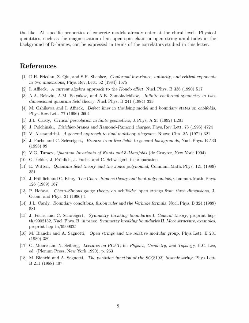
Next we discuss an example featuring an orientable surface with boundary; we compute theone-point amplitude for a bulk field j on a disk D with boundary condition a. Again the spaceof blocks is one-dimensional. Our task is then to compare the Wilson graph of figure 4 with thestandard basis that is displayed in figure 5. (In the present context, this particular conformalblock is often called an ‘Ishibashi state’). We now obtain the three-sphere by glueing with asingle three-ball. When applied to the graph of figure 5, we get the unknot with label j in S3,for which the partition function is S0,j. In the case of figure 4 we get a pair of linked Wilsonlines with labels a and j in S3; the value of the link invariant for this graph is Sa,j . Comparisonthus shows that the correlation function is Sa,j/S0,j times the standard two-point block on thesphere,

C(Da; j) = (Sa,j/S0,j) · B(S2; j, j∗) . (4)

5

Taking into account the normalization of the bulk fields as obtained in formula (3), we recoverthe known result that the correlator for a canonically normalized bulk field j on a disk withboundary condition a is Sa,j/

√

S0,j times the standard two-point block on the sphere. (Thisrelation forms the basis of the so-called boundary state formalism [14].)

��������������������������������������������������������������������������������������������������������������������������������������������������������������������������������������������������������������������������������������������������������������������������

��������������������������������������������������������������������������������������������������������������������������������������������������������������������������������������������������������������������������������������������������������������������������

������������������������������������������������������������������������������������������������������������������������������������������������������������������������������������������������������������������������������������������������������������

������������������������������������������������������������������������������������������������������������������������������������������������������������������������������������������������������������������������������������������������������������

Figure 4: C(Da; j)

Figure 5: B(S2; j, j∗)

As a third example, we study again a one-point correlator of a (bulk) field j, now on thecross-cap RP

2, which does not have a boundary, but is non-orientable. The latter propertyforces us to be careful with the framing. The structure constants are obtained by comparingthe correlator C(RP2; j) with the ‘cross-cap state’ ψj . This state is defined in figure 6; it issimilar to the basis element B(S2; j, j∗) of the two-point blocks on S2, but now the Wilson linein the three-ball has a non-trivial framing, and accordingly in figure 6 we have drawn a ribboninstead of a line. A priori we could twist the line either by +π, thereby obtaining some stateψ+j , or by −π and obtain another state ψ−

j . These two vectors differ by a factor of e2πi∆j , with∆j the conformal weight of j. Salomonically, we define the cross-cap state as

ψj := e−πi∆j ψ−

j = eπi∆j ψ+j . (5)

Again the comparison of the correlator C(RP2; j) with the standard basis ψj is carried out byglueing a three-ball with a Wilson line to the ball of figure 6. In contrast to the previous cases,however, this line is given a non-trivial framing; choosing the framing in such a way that thetwist of the cross-cap state is undone, glueing the ball to the cross-cap state yields S3 with theunknot, with partition function Z(S3; j) =S0,j.

As already mentioned, glueing the three-ball to the connecting manifold of the cross-capyields SO(3). It is also known that SO(3) can be obtained from S3 by a surgery on the unknotwith framing −2. (Following how the framed graph is mapped by the surgery, one may visualizethe situation as in figure 7.) Taking all framings properly into account, we obtain

Z(SO(3); j) = T1/20

∑

k

S0,k (Tk)2 Sk,j T

1/2j = P0,j (6)

6

(with Tj ≡ e2πi(∆j−c/24)) for the invariant of this three-manifold, where in the second equality weexpressed the result through the matrix [18] P := T 1/2ST 2ST 1/2. We have thereby recoveredthe known formula

C(RP2; j) = (P0,j/S0,j) · ψj (7)

for the one-point correlator on the cross-cap.

j

k

j

Figure 6: The state ψ+j =e−πi∆jψj

Figure 7: A visualization of C(RP2; j)

As a final example, consider three boundary fields i, j, k on a disk. The relevant Wilsongraph in the three-ball is of the type shown in figure 1, without any vertical Wilson linesalong connecting intervals; it consists of a circular line (with segments labelled a, b, c) withthree short Wilson lines (labelled i, j, k) attached to it. We must compare it to the standardbasis for three-point blocks on the sphere, which is a Mercedes star shaped junction. Thiscomparison can be made by performing a single fusing operation, followed by a contractionof the loop. For boundary fields, it is natural to define the correlation functions as linearforms on the degeneracy spaces for boundary operators. Denoting a basis of the degeneracyspace for the boundary operator ψac

i by {eα[ica∗]}, normalized by the quantum trace condition

tr (eα[ica∗] eβ[i

∗ac∗]) = δα,β, we find that

C(Da,b,c; i, j, k) (eα[ica∗] ⊗ eβ[jab∗] ⊗ eγ[kbc∗]) =∑

κ

S0,0

Sk,0{ i c a

b∗ j∗ k∗}αβ

γκeκ[kji] , (8)

where the symbol { i j kl m n}

αβ

γδdenotes a fusing matrix (or quantum 6j-symbol) [17, 9].

One important conclusion we can draw from our results is that the construction of correlationfunctions from conformal blocks can be performed in a completely model-independent manner.All structure constants, for any arbitrary conformal field theory, can be expressed in termsof purely chiral data, such as conformal weights, the modular S-matrix, fusing matrices and

7

the like. All specific properties of concrete models already enter at the chiral level. Physicalquantities, such as the magnetization of an open spin chain or open string amplitudes in thebackground of D-branes, can be expressed in terms of the correlators studied in this letter.

References

[1] D.H. Friedan, Z. Qiu, and S.H. Shenker, Conformal invariance, unitarity, and critical exponents

in two dimensions, Phys.Rev. Lett. 52 (1984) 1575

[2] I. Affleck, A current algebra approach to the Kondo effect, Nucl. Phys. B 336 (1990) 517

[3] A.A. Belavin, A.M. Polyakov, and A.B. Zamolodchikov, Infinite conformal symmetry in two-

dimensional quantum field theory, Nucl. Phys. B 241 (1984) 333

[4] M. Oshikawa and I. Affleck, Defect lines in the Ising model and boundary states on orbifolds,Phys.Rev. Lett. 77 (1996) 2604

[5] J.L. Cardy, Critical percolation in finite geometries, J. Phys. A 25 (1992) L201

[6] J. Polchinski, Dirichlet-branes and Ramond--Ramond charges, Phys.Rev. Lett. 75 (1995) 4724

[7] V. Alessandrini, A general approach to dual multiloop diagrams, Nuovo Cim. 2A (1971) 321

[8] J. Fuchs and C. Schweigert, Branes: from free fields to general backgrounds, Nucl. Phys. B 530(1998) 99

[9] V.G. Turaev, Quantum Invariants of Knots and 3-Manifolds (de Gruyter, New York 1994)

[10] G. Felder, J. Frohlich, J. Fuchs, and C. Schweigert, in preparation

[11] E. Witten, Quantum field theory and the Jones polynomial, Commun.Math. Phys. 121 (1989)351

[12] J. Frohlich and C. King, The Chern--Simons theory and knot polynomials, Commun.Math. Phys.126 (1989) 167

[13] P. Horava, Chern--Simons gauge theory on orbifolds: open strings from three dimensions, J.Geom. and Phys. 21 (1996) 1

[14] J.L. Cardy, Boundary conditions, fusion rules and the Verlinde formula, Nucl. Phys. B 324 (1989)581

[15] J. Fuchs and C. Schweigert, Symmetry breaking boundaries I. General theory, preprint hep-th/9902132, Nucl. Phys. B, in press; Symmetry breaking boundaries II. More structure, examples,preprint hep-th/9909025

[16] M. Bianchi and A. Sagnotti, Open strings and the relative modular group, Phys. Lett. B 231(1989) 389

[17] G. Moore and N. Seiberg, Lectures on RCFT, in: Physics, Geometry, and Topology, H.C. Lee,ed. (Plenum Press, New York 1990), p. 263

[18] M. Bianchi and A. Sagnotti, The partition function of the SO(8192) bosonic string, Phys. Lett.B 211 (1988) 407

8