Embed Size (px)
Citation preview

ASAP Reference Guide
ASAP | Contents | 2
Contents
ASAP Reference Guide - Introduction.................................................................12
Achieving Optimal Performance in ASAP...........................................................13
Setting the Working Directory..............................................................................14
Commands and Macros (A).................................................................................. 15a,b,c... (ASAP Command Argument).................................................................................................................15ABEL (ASAP Command).................................................................................................................................. 16ABERRATIONS (ASAP Command).................................................................................................................16ABG (ASAP Command).................................................................................................................................... 18$ABORT (ASAP Macro)................................................................................................................................... 19ABSORB (ASAP Command Argument)........................................................................................................... 20ACCURACY (ASAP Command)...................................................................................................................... 20ACTIVITY (ASAP Command Argument)........................................................................................................ 21AFOCAL (ASAP Command).............................................................................................................................22ALIGN (ASAP Command)................................................................................................................................ 23ALLOWED (ASAP Command).........................................................................................................................24ALTER (Edge Modifier) (ASAP Command).................................................................................................... 25ALTER (Lens Modifier) (ASAP Command).....................................................................................................26ALTER (Surface Modifier) (ASAP Command)................................................................................................ 27ANALYZE (ASAP Command)..........................................................................................................................28ANGLES (ASAP Command Argument)........................................................................................................... 28ANGLES (ASAP Command).............................................................................................................................29APODIZE (USERAPOD) (ASAP Command)...................................................................................................29APPEND (ASAP Command)............................................................................................................................. 31ARC (ASAP Command).................................................................................................................................... 32$ARGS (ASAP Macro)...................................................................................................................................... 32ARRAY (ASAP Command)...............................................................................................................................33ARRAY NONLINEAR (ASAP Command)...................................................................................................... 34ARROWS (ASAP Command)............................................................................................................................36ASCALE (ASAP Command)............................................................................................................................. 36$ASK (ASAP Macro).........................................................................................................................................37ASYM (ASAP Command)................................................................................................................................. 37AVERAGE (ASAP Command)..........................................................................................................................38AXICONIC (ASAP Command)......................................................................................................................... 39AXIS (ASAP Command)................................................................................................................................... 40
Commands and Macros (B)...................................................................................42BEAMS (ASAP Command)...............................................................................................................................42$BEEP (ASAP Macro)....................................................................................................................................... 42BEND (ASAP Command)..................................................................................................................................43BEZIER (ASAP Command)...............................................................................................................................43BIC (ASAP Command)......................................................................................................................................44BICONIC (ASAP Command)............................................................................................................................ 45
ASAP | Contents | 3
BILATERAL (ASAP Command)...................................................................................................................... 46BIN (ASAP Command)......................................................................................................................................47BOUNDS (ASAP Command)............................................................................................................................ 47BRANCH (ASAP Command)............................................................................................................................ 48BSDFDATA (ASAP Command)........................................................................................................................49
Commands and Macros (C).................................................................................. 53CADEXPORT (ASAP Command).....................................................................................................................53CARTOVAL (ASAP Command).......................................................................................................................54$CASE (ASAP Macro).......................................................................................................................................55CHARACTER (ASAP Command).................................................................................................................... 55CHROMATICITY (ASAP Command).............................................................................................................. 56
SOM Option Matrix for CIE-CHROMATICITY Commands............................................................... 58CIE (ASAP Command)...................................................................................................................................... 59
SOM Option Matrix for CIE-CHROMATICITY Commands............................................................... 60CIELAB (ASAP Command).............................................................................................................................. 61CIELUV (ASAP Command).............................................................................................................................. 62CIEUVW (ASAP Command).............................................................................................................................63$CLEAR (ASAP Macro)....................................................................................................................................64CLIP (ASAP Command Argument).................................................................................................................. 64CLIP (ASAP Command)....................................................................................................................................65COARSEN (ASAP Command).......................................................................................................................... 66COATINGS LAYERS (ASAP Command)........................................................................................................67COATINGS MODELS (ASAP Command).......................................................................................................68COATINGS PROPERTIES (ASAP Command)................................................................................................69COLLECTION (ASAP Command)....................................................................................................................70COLORS (ASAP Command Argument)........................................................................................................... 71COLORS (ASAP Command).............................................................................................................................72COMBINE (ASAP Command).......................................................................................................................... 74COMPOSITE (Edge Modifier) (ASAP Command)...........................................................................................74COMPOSITE (Lens Modifier) (ASAP Command)........................................................................................... 75CONDUIT (ASAP Command)...........................................................................................................................76CONIC (ASAP Command)................................................................................................................................ 76CONSIDER (ASAP Command).........................................................................................................................77CONTOUR (ASAP Command)......................................................................................................................... 78$COPY (ASAP Macro)...................................................................................................................................... 79CORNER (ASAP Command)............................................................................................................................ 80CPE (ASAP Command)..................................................................................................................................... 80CRYSTAL (ASAP Command Argument)......................................................................................................... 82CUTOFF (ASAP Command)............................................................................................................................. 83CVF (ASAP Command).....................................................................................................................................83
Commands and Macros (D).................................................................................. 86$DATIM (ASAP Macro)....................................................................................................................................86$DBG (ASAP Macro)........................................................................................................................................ 86DECOMPOSE (ASAP Command).................................................................................................................... 86DEFORM (ASAP Command)............................................................................................................................ 88DIMENSIONS (ASAP Command).................................................................................................................... 89DIRECTIONAL (ASAP Command)..................................................................................................................90$DISP (ASAP Macro)........................................................................................................................................ 90DISPLAY (ASAP Command)............................................................................................................................91DMAP (ASAP Command)................................................................................................................................. 93$DO (ASAP Macro)........................................................................................................................................... 93DOMACROS (ASAP Command)...................................................................................................................... 94
ASAP | Contents | 4
DOME (ASAP Command).................................................................................................................................95DOPL (ASAP Command).................................................................................................................................. 95DOUBLET (ASAP Command).......................................................................................................................... 96DRAWING (ASAP Command)......................................................................................................................... 97DUMP (ASAP Command)................................................................................................................................. 98
Commands and Macros (E)...................................................................................99$ECHO (ASAP Macro)......................................................................................................................................99EDGES/CURVES (ASAP Command)............................................................................................................... 99$EDIT (ASAP Macro)........................................................................................................................................99ELLIPSE (ASAP Command)........................................................................................................................... 100ELLIPSOID (ASAP Command)...................................................................................................................... 101EMITTING (ASAP Command)....................................................................................................................... 102EMITTING BOX/SPHEROID (ASAP Command)......................................................................................... 103EMITTING CONE/PYRAMID (ASAP Command)........................................................................................103EMITTING DATA (ASAP Command)........................................................................................................... 104EMITTING DISK/RECTANGLE (ASAP Command).................................................................................... 106EMITTING ENTITY or OBJECT (ASAP Command)................................................................................... 107EMITTING EULUMDAT (ASAP Command)................................................................................................108EMITTING FILAMENT (ASAP Command).................................................................................................. 108EMITTING HELIX (ASAP Command).......................................................................................................... 109EMITTING IES (ASAP Command)................................................................................................................ 110EMITTING RAYS (ASAP Command)........................................................................................................... 111ENCLOSED (ASAP Command)......................................................................................................................112END (ASAP Command).................................................................................................................................. 112ENTITIES (ASAP Command)......................................................................................................................... 113$ERR (ASAP Macro)....................................................................................................................................... 114EULUMDATFILE (ASAP Command)............................................................................................................114$EVAL (ASAP Macro).................................................................................................................................... 115$EXIT (ASAP Macro)......................................................................................................................................116$EXP (ASAP Macro)....................................................................................................................................... 117EXPLICIT (ASAP Command).........................................................................................................................117EXPLODE (ASAP Command)........................................................................................................................ 118EXTEND (ASAP Command)...........................................................................................................................119EXTREMES (ASAP Command)......................................................................................................................119
Commands and Macros (F).................................................................................121FACETS (ASAP Command)............................................................................................................................121$FAST (ASAP Macro)..................................................................................................................................... 121$FCN (ASAP Macro)....................................................................................................................................... 122$FF (ASAP Macro).......................................................................................................................................... 123FFAD (ASAP Command)................................................................................................................................ 123FFT (ASAP Command)....................................................................................................................................124FIELD (ASAP Command)............................................................................................................................... 125FIELDBPM (ASAP Command).......................................................................................................................129FIELDSUM (ASAP Command).......................................................................................................................131FITTED (ASAP Command).............................................................................................................................132FLUX (ASAP Command)................................................................................................................................ 134FMAP (ASAP Command)................................................................................................................................134FOCUS (ASAP Command)..............................................................................................................................135FOLD (ASAP Command)................................................................................................................................ 137FORM (ASAP Command)............................................................................................................................... 138FRESNEL (ASAP Command)......................................................................................................................... 138FTSIZE (ASAP Command)..............................................................................................................................140
ASAP | Contents | 5
Commands and Macros (G)................................................................................ 141GAUSSIAN (ASAP Command)...................................................................................................................... 141GENERAL (ASAP Command)........................................................................................................................ 142GET (ASAP Command)...................................................................................................................................145$GO (ASAP Macro)......................................................................................................................................... 147$GRAB (ASAP Macro)....................................................................................................................................148GRAPH (ASAP Command)............................................................................................................................. 148GRID DATA (ASAP Command).................................................................................................................... 149GRID ELLIPTIC (ASAP Command).............................................................................................................. 150GRID HEX (ASAP Command)....................................................................................................................... 151GRID OBJECT (ASAP Command)................................................................................................................. 152GRID POLAR (ASAP Command).................................................................................................................. 153GRID RECT (ASAP Command)..................................................................................................................... 154GRID WINDOW (ASAP Command).............................................................................................................. 155GRIN (ASAP Command Argument)............................................................................................................... 156GROUP (ASAP Command)............................................................................................................................. 156$GUI (ASAP Macro)........................................................................................................................................157GUM (ASAP Command)................................................................................................................................. 161
Commands and Macros (H)................................................................................ 164HALT (ASAP Command)................................................................................................................................ 164HARVEY (ASAP Command).......................................................................................................................... 165HEADER (ASAP Command).......................................................................................................................... 166HELIX (ASAP Command)...............................................................................................................................167$HELP (ASAP Macro).....................................................................................................................................168HISTOGRAM (ASAP Command)...................................................................................................................168HISTORY (ASAP Command)......................................................................................................................... 169HORN (ASAP Command)............................................................................................................................... 173
Commands and Macros (I)..................................................................................175IDEAL (ASAP Command)...............................................................................................................................175IESFILE (ASAP Command)............................................................................................................................ 176$IF (ASAP Macro)........................................................................................................................................... 178$IF THEN (ASAP Macro)............................................................................................................................... 179IMAGE Curve/Edge (ASAP Command)......................................................................................................... 180IMAGE (Global Point) (ASAP Command)..................................................................................................... 180IMAGE (Ray Positions) (ASAP Command)................................................................................................... 181IMMERSE (ASAP Command)........................................................................................................................ 181IMPORT (ASAP Command)............................................................................................................................182INTERFACE (ASAP Command).....................................................................................................................183INTERFACE POLARIZATION (Polarization Modifiers) (ASAP Command)...............................................185INTERFACE REPEAT (ASAP Command).................................................................................................... 186INVERT (ASAP Command)............................................................................................................................ 187$IO (ASAP Macro)...........................................................................................................................................187IRRADIANCE (ASAP Command).................................................................................................................. 190ISOMETRIC (ASAP Command)..................................................................................................................... 190$ITER (ASAP Macro)......................................................................................................................................191
Commands and Macros (JKL)............................................................................193JONES (ASAP Command)...............................................................................................................................193KCORRELATION (ASAP Command)............................................................................................................194
ASAP | Contents | 6
LAMBERTIAN (ASAP Command).................................................................................................................195LCC (ASAP Command)...................................................................................................................................195$LEAVE (ASAP Macro)..................................................................................................................................198LENSES (ASAP Command)............................................................................................................................ 198LEVEL (ASAP Command).............................................................................................................................. 199LIGHTS (ASAP Command)............................................................................................................................ 200LIMITS (ASAP Command)............................................................................................................................. 200LINE (ASAP Command)..................................................................................................................................202LIST (ASAP Command).................................................................................................................................. 202LIST ELLIPSE (ASAP Command)................................................................................................................. 203LIST INTEGER (ASAP Command)................................................................................................................204LIST (Parabasal Ray Data) (ASAP Command)...............................................................................................204LIST RAYS (ASAP Command)...................................................................................................................... 204$LOC (ASAP Macro).......................................................................................................................................205LOCAL (ASAP Command)............................................................................................................................. 206LSQFIT (ASAP Command)............................................................................................................................. 208
Commands and Macros (M)................................................................................209MANGIN (ASAP Command).......................................................................................................................... 209MAP (ASAP Command)..................................................................................................................................210MATRIX (ASAP Command)...........................................................................................................................211MEDIA (ASAP Command)..............................................................................................................................212
MEDIA Command Coefficients........................................................................................................... 214MEDIA ABSORB (ASAP Command)............................................................................................................ 215MEDIA BIAXIAL (ASAP Command)............................................................................................................216MEDIA CRYSTAL (ASAP Command).......................................................................................................... 217MEDIA GRIN (ASAP Command).................................................................................................................. 218MEDIA SCATTER (ASAP Command)...........................................................................................................220MEDIA USER (ASAP Command).................................................................................................................. 221$MENU (ASAP Macro)................................................................................................................................... 222MESH (ASAP Command)................................................................................................................................223MICROSTRUCTURE (ASAP Command)...................................................................................................... 223MINIMIZE (ASAP Command)........................................................................................................................225MINMAX (ASAP Command Argument)........................................................................................................ 227MIRROR (ASAP Command)...........................................................................................................................227MISSED (ASAP Command)............................................................................................................................ 228MODEL (ASAP Command Argument)........................................................................................................... 228MODELS (ASAP Command).......................................................................................................................... 229MODIFY (ASAP Command)...........................................................................................................................230MOVE (ASAP Command)...............................................................................................................................231MOVE PARABASALS (ASAP Command)....................................................................................................232MOVE TO FOCI (ASAP Command)..............................................................................................................233MOVE TO PLANE (ASAP Command).......................................................................................................... 233MOVE TO POINT (ASAP Command)........................................................................................................... 233MOVE TO SPHERE (ASAP Command)........................................................................................................ 234$MSGS (ASAP Macro)....................................................................................................................................234MUELLER (ASAP Command)........................................................................................................................234MULTIPLE (ASAP Command).......................................................................................................................236
Commands and Macros (N-O)............................................................................ 238$NEXT (ASAP Macro).................................................................................................................................... 238NONLINEAR (ASAP Command)................................................................................................................... 238NORMALIZE (ASAP Command)................................................................................................................... 241NUMBERS (ASAP Command)....................................................................................................................... 241

ASAP | Contents | 7
OBJECT (ASAP Command)............................................................................................................................ 242OBLIQUE (ASAP Command)......................................................................................................................... 243OFFSET (ASAP Command)............................................................................................................................ 244OPDMAP (ASAP Command).......................................................................................................................... 244OPTICAL (ASAP Command)..........................................................................................................................245OVAL (ASAP Command)................................................................................................................................247OVERLAY (ASAP Command Argument)...................................................................................................... 247
Commands and Macros (P).................................................................................249$PAGE (ASAP Macro).................................................................................................................................... 249PARABASAL (ASAP Command)...................................................................................................................249PARAMETERIZE (ASAP Command)............................................................................................................ 250PARTICLES (ASAP Command)..................................................................................................................... 251PATCHES (ASAP Command).........................................................................................................................252$PATH (ASAP Macro).................................................................................................................................... 253PATHS (ASAP Command).............................................................................................................................. 253PERFECT (ASAP Command)..........................................................................................................................255PHYSICAL (ASAP Command)....................................................................................................................... 256PICTURE (ASAP Command).......................................................................................................................... 256PIXELS (ASAP Command Argument)............................................................................................................257PIXELS (ASAP Command)............................................................................................................................. 257PLACE (CURVE/EDGE) (ASAP Command).................................................................................................258PLACE (Global Coordinate) (ASAP Command)............................................................................................ 258PLACE (Relative to Entity) (ASAP Command)..............................................................................................259PLANE (ASAP Command)..............................................................................................................................260PLANE NORMAL (ASAP Command)........................................................................................................... 261PLANE POINTS (ASAP Command)...............................................................................................................261$PLAY (ASAP Macro).................................................................................................................................... 262Plotting Commands...........................................................................................................................................262PLOT3D (ASAP Command)............................................................................................................................263PLOT BEAMS (ASAP Command)..................................................................................................................263PLOT CURVES (ASAP Command)................................................................................................................264PLOT EDGES (ASAP Command).................................................................................................................. 265PLOT ENTITIES (ASAP Command)..............................................................................................................265PLOT FACETS (ASAP Command).................................................................................................................266PLOT LENSES (ASAP Command).................................................................................................................268PLOT LIMITS (ASAP Command).................................................................................................................. 269PLOT LOCAL (ASAP Command).................................................................................................................. 269PLOT MESHES (ASAP Command)................................................................................................................270PLOT POLARIZATION (ASAP Command).................................................................................................. 271PLOT RAYS (ASAP Command).....................................................................................................................272PLOT SURFACES (ASAP Command)........................................................................................................... 272PLOT (ASAP Command Argument)............................................................................................................... 273$PLOT (ASAP Macro).....................................................................................................................................274POINTS (2D) (ASAP Command)....................................................................................................................274POINTS (3D) (ASAP Command)....................................................................................................................275POLARIZ (ASAP Command)..........................................................................................................................277POLARIZ K (Reference Ray Direction) (ASAP Command)..........................................................................278POLARIZ MODE (ASAP Command).............................................................................................................279POLARIZ (Polarization Vector) (ASAP Command).......................................................................................279POLARIZ RANDOM (ASAP Command).......................................................................................................280POLARIZ TREF (Transverse Reference Direction) (ASAP Command)........................................................ 281POLYNOMIAL/TRINOMIAL/BINOMIAL (ASAP Command)....................................................................282PostScript File Utility (PSCRIP) (ASAP Command)...................................................................................... 284PRINT (ASAP Command)............................................................................................................................... 285
ASAP | Contents | 8
PRINT (Polarization Models) (ASAP Command)...........................................................................................289PROFILES (ASAP Command)........................................................................................................................ 290PUT (ASAP Command)................................................................................................................................... 291
Commands and Macros (R)................................................................................ 294RACETRACK (ASAP Command)...................................................................................................................294RADIAL (ASAP Command)............................................................................................................................294RADIANT (ASAP Command).........................................................................................................................295$RAN (ASAP Macro)...................................................................................................................................... 297RANGE (ASAP Command).............................................................................................................................297RAWDATA (ASAP Command)...................................................................................................................... 298RAY (ASAP Command).................................................................................................................................. 298RAYS (ASAP Command)................................................................................................................................ 300RAYSET (ASAP Command)........................................................................................................................... 300$READ (ASAP Macro)....................................................................................................................................302RECTANGLE (ASAP Command)................................................................................................................... 302REDEFINE (ASAP Command)....................................................................................................................... 303REDUCE (ASAP Command)...........................................................................................................................304$REG (ASAP Macro).......................................................................................................................................304REMOVE (ASAP Command)..........................................................................................................................305RENDER (ASAP Command)...........................................................................................................................305RENORM (ASAP Command)..........................................................................................................................306REPEAT (ASAP Command)............................................................................................................................307REPLICATE (ASAP Command)..................................................................................................................... 308REPLOT (ASAP Command)............................................................................................................................308RESET (ASAP Command).............................................................................................................................. 309RESTRICT (ASAP Command)........................................................................................................................310RETURN (ASAP Command)...........................................................................................................................310REVERSE (ASAP Command).........................................................................................................................310REVOLUTION (ASAP Command)................................................................................................................. 311REVOLUTION (Fitted) (ASAP Command)....................................................................................................311RIGHT (ASAP Command).............................................................................................................................. 312RMS (ASAP Command).................................................................................................................................. 313ROOF (ASAP Command)................................................................................................................................ 314ROTATE (ASAP Command)...........................................................................................................................314ROUGHNESS (ASAP Command)...................................................................................................................315ROUNDED (ASAP Command)....................................................................................................................... 317RPM (ASAP Command).................................................................................................................................. 318RRM (ASAP Command)..................................................................................................................................319
Commands and Macros (S)................................................................................. 322SAG (ASAP Command)...................................................................................................................................322SAMPLED (ASAP Command)........................................................................................................................ 323SAMPLED (Cylindrical) (ASAP Command).................................................................................................. 325SAVE (ASAP Command)................................................................................................................................ 326SAWTOOTH (ASAP Command).................................................................................................................... 326SCALE (ASAP Command).............................................................................................................................. 327SCALE FROM (ASAP Command)................................................................................................................. 328SCATTER (ASAP Command Argument)....................................................................................................... 329SCATTER RANDOM or MODEL (ASAP Command).................................................................................. 329SCATTER REPEAT (ASAP Command).........................................................................................................331SCATTER RMS/BSDF (ASAP Command).................................................................................................... 331$SCR (ASAP Macro)....................................................................................................................................... 332SEARCH (ASAP Command)...........................................................................................................................333
ASAP | Contents | 9
$SEARCH (ASAP Macro)............................................................................................................................... 335SECTION (ASAP Command)..........................................................................................................................335SEED (ASAP Command).................................................................................................................................336SEGMENTS (ASAP Command)......................................................................................................................337SELECT (ASAP Command)............................................................................................................................ 337SEQUENCE (ASAP Command)......................................................................................................................340SET (ASAP Command)................................................................................................................................... 341SHAPE (ASAP Command).............................................................................................................................. 342SHIFT (ASAP Command)................................................................................................................................344SHOW (ASAP Command)...............................................................................................................................345$SHOW (ASAP Macro)................................................................................................................................... 346SINGLET (ASAP Command).......................................................................................................................... 346SKEW (ASAP Command)............................................................................................................................... 347SMOOTH (ASAP Command)..........................................................................................................................348SOLID (ASAP Command)...............................................................................................................................348SOURCE (ASAP Command)...........................................................................................................................349SOURCE POLYCHROMATIC (ASAP Command)....................................................................................... 350SOURCE WAVEFUNC (ASAP Command)................................................................................................... 353SPECTRUM (ASAP Command)......................................................................................................................354SPLINE, EXPLICIT 2D (ASAP Command)................................................................................................... 355SPLINE, GENERAL 3D (ASAP Command).................................................................................................. 356SPLIT (ASAP Command)................................................................................................................................ 356SPOTS (ASAP Command)...............................................................................................................................358SPREAD (ASAP Command)........................................................................................................................... 360$STAMP (ASAP Macro)..................................................................................................................................362STATS (ASAP Command).............................................................................................................................. 363STATS TRACE (ASAP Command)................................................................................................................ 363$STO/$RCL/&STO (ASAP Macro).................................................................................................................364STORE (ASAP Command).............................................................................................................................. 364SUBSET (ASAP Command)............................................................................................................................365SUM (ASAP Command)..................................................................................................................................365SUPERCONIC (ASAP Command)..................................................................................................................366SURFACES/FUNCTIONS (ASAP Command)............................................................................................... 367SWEEP (ASAP Command)..............................................................................................................................367$SYS (ASAP Macro)....................................................................................................................................... 368SYSTEM (ASAP Command)...........................................................................................................................369
Commands and Macros (T).................................................................................371TABLE (ASAP Command)..............................................................................................................................371TELESCOPE (ASAP Command).................................................................................................................... 371TERRAIN (ASAP Command)......................................................................................................................... 372TEST (ASAP Command)................................................................................................................................. 373TEXT (ASAP Command Argument)............................................................................................................... 374TEXTFILE (ASAP Command)........................................................................................................................ 375THRESHOLD (ASAP Command)...................................................................................................................377$TIC (ASAP Macro)........................................................................................................................................ 377TITLE (ASAP Command)................................................................................................................................378TORUS (ASAP Command)..............................................................................................................................378TOWARDS (ASAP Command).......................................................................................................................379TRACE (ASAP Command)..............................................................................................................................381TRANSPOSE (ASAP Command)....................................................................................................................383TREE (ASAP Command).................................................................................................................................383TUBE (ASAP Command)................................................................................................................................ 383
ASAP | Contents | 10
Commands and Macros (U)................................................................................ 386UNITS (ASAP Command)...............................................................................................................................386$UNVAR (ASAP Macro).................................................................................................................................387UPDATE (ASAP Command)...........................................................................................................................387APODIZE (USERAPOD) (ASAP Command).................................................................................................387USERAPOD ANGLES (ASAP Command).....................................................................................................389USERAPOD BOTH (ASAP Command)......................................................................................................... 391USERBSDF (ASAP Command)...................................................................................................................... 392USERCURVE (ASAP Command)...................................................................................................................395USERFUNC (ASAP Command)......................................................................................................................396USERSAG (ASAP Command)........................................................................................................................ 397UVSPACE (ASAP Command)........................................................................................................................ 398
Commands and Macros (V)................................................................................ 400VALUES (ASAP Command)...........................................................................................................................400VANES (ASAP Command)............................................................................................................................. 400VARIABLES (ASAP Command).................................................................................................................... 401VCAVITY (ASAP Command).........................................................................................................................402VERSION (ASAP Command)......................................................................................................................... 403VIEW (ASAP Command)................................................................................................................................ 403$VIEW (ASAP Macro).................................................................................................................................... 404VIOLATION (ASAP Command).....................................................................................................................405VOXELS (ASAP Command)...........................................................................................................................405VUFACETS (ASAP Command)...................................................................................................................... 406
Commands and Macros (W)............................................................................... 408$WAIT (ASAP Macro).................................................................................................................................... 408WARNINGS (ASAP Command)..................................................................................................................... 408WAVELENGTH(S) (ASAP Command)..........................................................................................................408WEDGE (ASAP Command)............................................................................................................................ 409WIDTHS (ASAP Command)........................................................................................................................... 410WINDOW (ASAP Command)......................................................................................................................... 411WRITE (ASAP Command).............................................................................................................................. 412
Commands and Macros (XYZ)........................................................................... 414XEQ (ASAP Command).................................................................................................................................. 414XMEMORY (ASAP Command)......................................................................................................................414XY[Z] and Other Plot Window Overrides (ASAP Command Argument)...................................................... 416ZERNIKE (ASAP Command)..........................................................................................................................416
Building Your System.......................................................................................... 419Achieving Optimal Performance in ASAP...................................................................................................... 419Setting the Working Directory......................................................................................................................... 420Building the Geometry..................................................................................................................................... 420
Define/Modify Entities or Single Entity Objects.................................................................................420Define/Modify Curve/Edge Entities..................................................................................................... 421Define/Modify Surface/Function Entities.............................................................................................422Define/Modify Lens Entities................................................................................................................ 424Create/Modify Media, Coatings, Scatter Models.................................................................................425Create/Modify Objects..........................................................................................................................426
ASAP | Contents | 11
Object Creation..................................................................................................................................... 428Building the Source.......................................................................................................................................... 428
Create Rays/Beams............................................................................................................................... 429Verifying the Geometry and Sources...............................................................................................................430
Setup Plots and Verify System............................................................................................................ 430Standard Plot Options...........................................................................................................................431Setup Beam Creation............................................................................................................................ 431Modify Ray/Beam Data........................................................................................................................432
Tracing the Rays...............................................................................................................................................432Tracing a Group of Rays or Beams..................................................................................................... 433Setup Trace........................................................................................................................................... 433Ray Tracing Data Saved by ASAP......................................................................................................434Trace Ray and Beams...........................................................................................................................435
Analyzing the Data........................................................................................................................................... 435Analyze Ray/Beam Data...................................................................................................................... 435Modify or Use Internal Ray/Beam Data as Input................................................................................ 436Calculate Diffraction/Propagation Effects............................................................................................436Save or Recover System Data and Control Execution........................................................................ 436Display/Modify Data Distributions...................................................................................................... 437
Kernel Capabilities Overview..............................................................................440Command Mode................................................................................................................................................440Examples of Command Scripts........................................................................................................................ 441Command Usage...............................................................................................................................................441Command Comment Strings............................................................................................................................ 442Command Description Notation.......................................................................................................................442Entries Repeated and Incremented................................................................................................................... 442Distribution Data Files Overview.................................................................................................................... 443Distribution Data Files Display........................................................................................................................443Distribution File Structure................................................................................................................................ 444File Naming Conventions in ASAP.................................................................................................................445Files Produced by ASAP..................................................................................................................................446File Structure of ASAP.................................................................................................................................... 448General Input Techniques.................................................................................................................................448Input Records.................................................................................................................................................... 450Mathematical Functions Supported.................................................................................................................. 450Mathematical Operators....................................................................................................................................452Registers for Storing Arithmetic Results......................................................................................................... 453Single- and Double-Precision Numbers........................................................................................................... 454Specifying Complex Numbers..........................................................................................................................454Variables............................................................................................................................................................454
Variable Substitution............................................................................................................................ 454Externally Named Variables.................................................................................................................455Internally Named Variables..................................................................................................................455
Quick Reference Guide........................................................................................ 457ASAP Syntax - Quick Reference.....................................................................................................................457Optical System Model - Quick Reference....................................................................................................... 457Verifying Optical System Model - Quick Reference.......................................................................................458Source Models - Quick Reference................................................................................................................... 459Verifying Source Model - Quick Reference.................................................................................................... 460Ray Tracing and Analysis - Quick Reference................................................................................................. 462Miscellaneous Useful Commands - Quick Reference..................................................................................... 462Macro Formatting - Quick Reference.............................................................................................................. 462
ASAP | ASAP Reference Guide - Introduction | 12
ASAP Reference Guide - Introduction
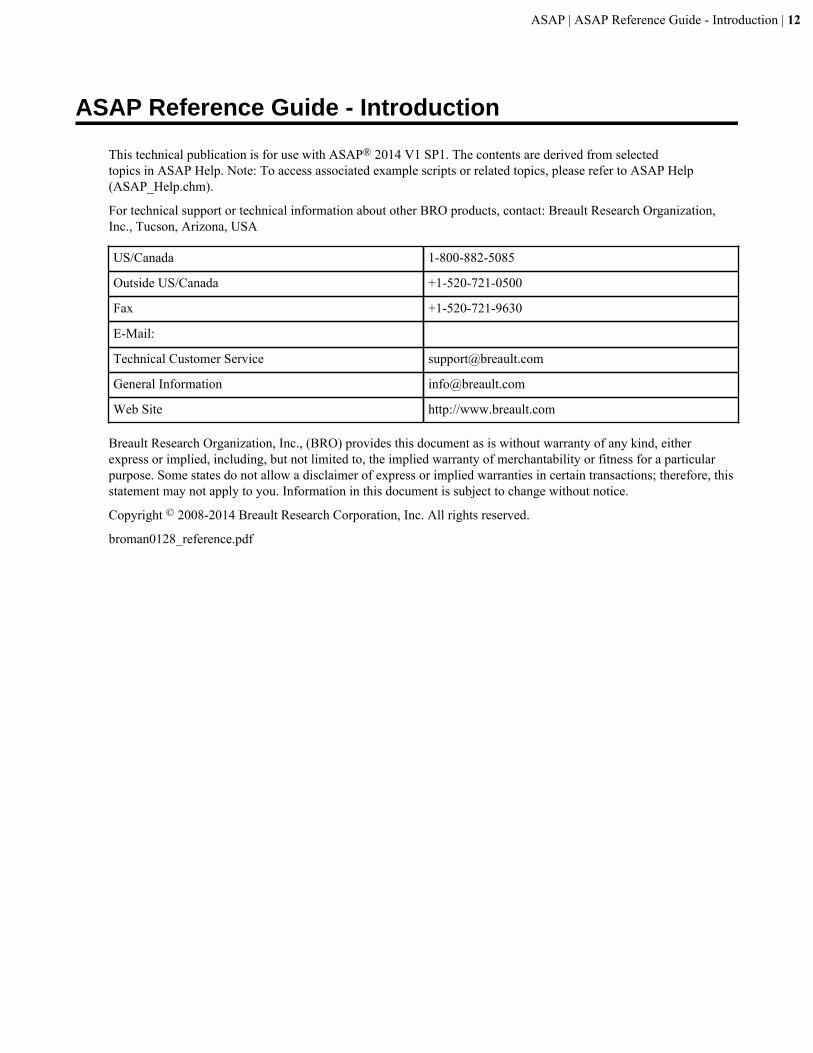
This technical publication is for use with ASAP® 2014 V1 SP1. The contents are derived from selectedtopics in ASAP Help. Note: To access associated example scripts or related topics, please refer to ASAP Help(ASAP_Help.chm).
For technical support or technical information about other BRO products, contact: Breault Research Organization,Inc., Tucson, Arizona, USA
US/Canada 1-800-882-5085
Outside US/Canada +1-520-721-0500
Fax +1-520-721-9630
E-Mail:
Technical Customer Service [email protected]
General Information [email protected]
Web Site http://www.breault.com
Breault Research Organization, Inc., (BRO) provides this document as is without warranty of any kind, eitherexpress or implied, including, but not limited to, the implied warranty of merchantability or fitness for a particularpurpose. Some states do not allow a disclaimer of express or implied warranties in certain transactions; therefore, thisstatement may not apply to you. Information in this document is subject to change without notice.
Copyright © 2008-2014 Breault Research Corporation, Inc. All rights reserved.
broman0128_reference.pdf
ASAP | Achieving Optimal Performance in ASAP | 13
Achieving Optimal Performance in ASAP
When determining your computer requirements, BRO encourages you to select an operating system that supportsoptimal performance for ASAP, and uses processor resources intensively for its computation, analysis, and graphicaloutput.
In particular, if you are running ASAP on Windows 7 operating systems with 64-bit versions, you can achieveoptimal performance from ASAP by adding as much memory as your budget allows. These operating systemsautomatically cache the virtual.pgs file in RAM up to the available amount of RAM memory. The virtual.pgs filecontains the rays used in the simulation. This is the file that ASAP uses to read and write rays during ray tracing, andit accesses this file for other analyses requiring ray data.
As a general rule, each ray of an incoherent extended source uses approximately 64 bytes of memory. If you knowthe number of rays in your source, you can use this simple relationship to estimate the size of the virtual.pgs file. Forexample, if you create 70 million rays, ASAP uses approximately 4.5 GB of available memory. If your initial sourcesize exceeds the available memory, ASAP uses the hard disk space, which is considerably slower and consequentlyaffects certain performances. Similarly, some simulations such as deterministic stray light analyses create rays andadd to the size of the virtual.pgs file.
The Windows operating system in 32-bit versions limits the memory available to 2 GB, regardless of the totalinstalled RAM. The operating system also requires memory of its own. A system with 2 GB of RAM typically canmake, at most, slightly over 1 GB of RAM available for ray data, before forcing ASAP to switch to a virtual.pgs fileon disk.
For faster speed, you may want to consider using SSD (solid-state drive) disks, regardless of the Windows operatingsystem, instead of traditional magnetic disks such as hard disk drives (HDDs). If ASAP runs out of available systemmemory, it uses disk storage. Therefore, ASAP performance improves with the speed of the disk drive systems.
ASAP | Setting the Working Directory | 14
Setting the Working Directory
The Working Directory in ASAP is the location where files are stored when you perform tasks such as runningscripts or translating files. This topic describes the default locations of this directory in Windows XP and Windows7 systems, which are different. Default settings are the recommended locations. The topic also describes how to set auser-designated location.
BRO recommends that you use the default settings for the Working Directory. Do not use a shared network drivelocation.
The default settings differ in Windows XP and Windows 7 systems. In Windows XP systems, alldirectories are writable, and the default location of the ASAP Working Directory is C:\Program Files\ASAPxxxxVx\Projects, where xxxxVx indicates the ASAP version you are using; for example, ASAP2014V1.In Windows 7 systems, security restrictions limit the location of writable files, and the Working Directory path that iswritable in Windows XP is not writable in Windows 7. For this reason, the default location of the Working Directoryin Windows 7 is C:\Users\username\AppData\Local\Breault Research Organization\ASAPxxxx.x\Projects, where ASAPxxxx.x indicates the ASAP version you are using; for example, 1404.1,where 14=year, and 01=version.
To set the Working Directory to a different location, the location must be writable. Follow these steps:
1. Click File, Set Working Directory in ASAP.2. In the Windows dialog box, select the folder to write the files, and click OK. Note: If you select a non-writable
location, unexpected behavior may result.
Assuming that the location of the Working Directory that you selected is writable, it is set until you change it.
ASAP | Commands and Macros (A) | 15
Commands and Macros (A)
Topics in this section of the Contents tab include ASAP commands and macros that begin with the letter “A”.
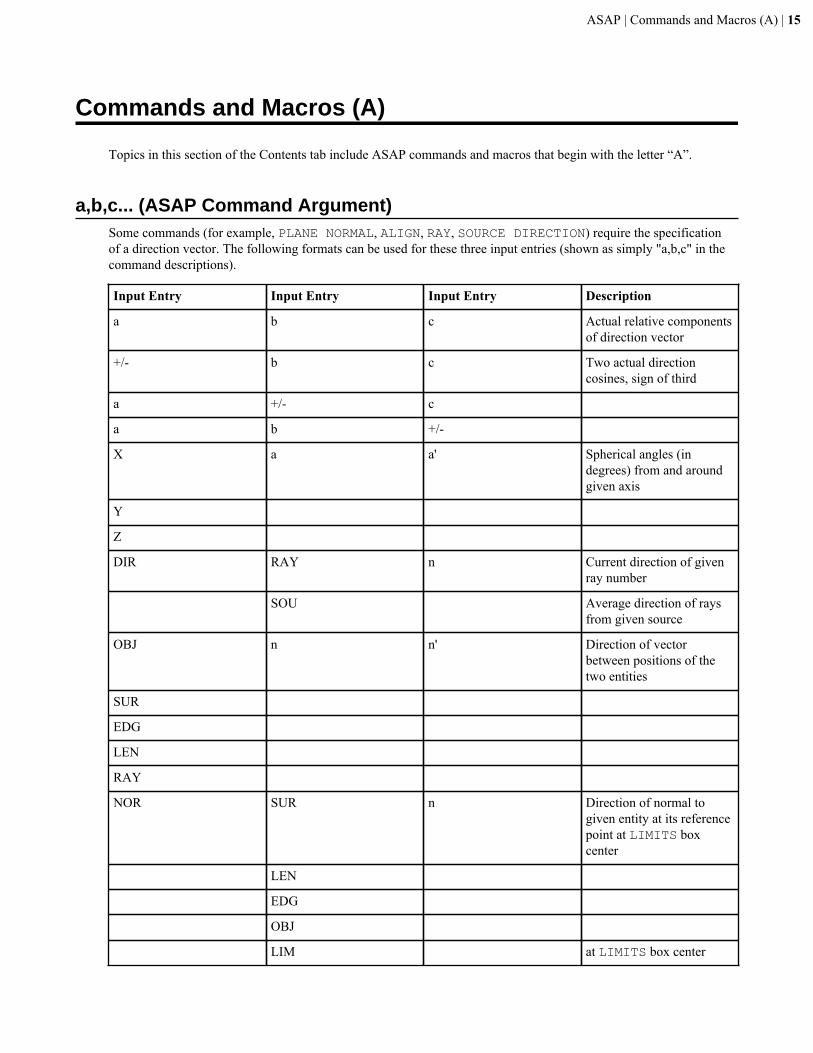
a,b,c... (ASAP Command Argument)Some commands (for example, PLANE NORMAL, ALIGN, RAY, SOURCE DIRECTION) require the specificationof a direction vector. The following formats can be used for these three input entries (shown as simply "a,b,c" in thecommand descriptions).
Input Entry Input Entry Input Entry Description
a b c Actual relative componentsof direction vector
+/- b c Two actual directioncosines, sign of third
a +/- c
a b +/-
X a a' Spherical angles (indegrees) from and aroundgiven axis
Y
Z
DIR RAY n Current direction of givenray number
SOU Average direction of raysfrom given source
OBJ n n' Direction of vectorbetween positions of thetwo entities
SUR
EDG
LEN
RAY
NOR SUR n Direction of normal togiven entity at its referencepoint at LIMITS boxcenter
LEN
EDG
OBJ
LIM at LIMITS box center
ASAP | Commands and Macros (A) | 16
Input Entry Input Entry Input Entry Description
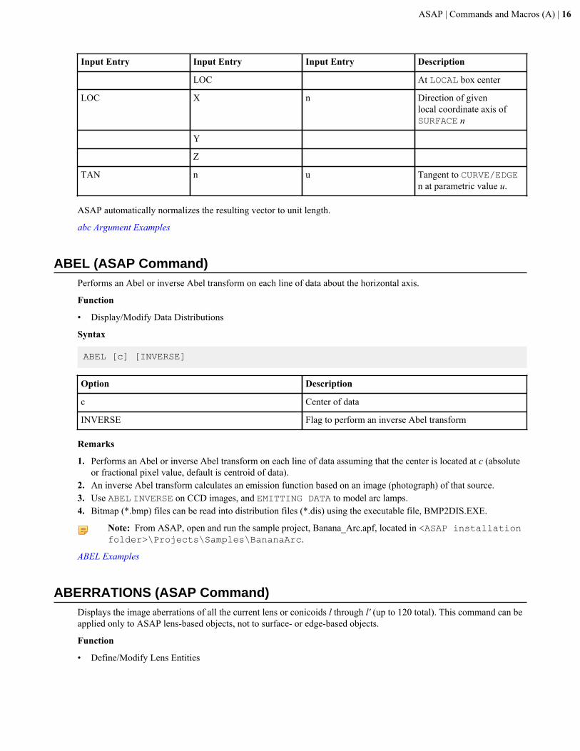
LOC At LOCAL box center
LOC X n Direction of givenlocal coordinate axis ofSURFACE n
Y
Z
TAN n u Tangent to CURVE/EDGEn at parametric value u.
ASAP automatically normalizes the resulting vector to unit length.
abc Argument Examples
ABEL (ASAP Command)Performs an Abel or inverse Abel transform on each line of data about the horizontal axis.
Function
• Display/Modify Data Distributions
Syntax
ABEL [c] [INVERSE]
Option Description
c Center of data
INVERSE Flag to perform an inverse Abel transform
Remarks
1. Performs an Abel or inverse Abel transform on each line of data assuming that the center is located at c (absoluteor fractional pixel value, default is centroid of data).
2. An inverse Abel transform calculates an emission function based on an image (photograph) of that source.3. Use ABEL INVERSE on CCD images, and EMITTING DATA to model arc lamps.4. Bitmap (*.bmp) files can be read into distribution files (*.dis) using the executable file, BMP2DIS.EXE.
Note: From ASAP, open and run the sample project, Banana_Arc.apf, located in <ASAP installationfolder>\Projects\Samples\BananaArc.
ABEL Examples
ABERRATIONS (ASAP Command)Displays the image aberrations of all the current lens or conicoids l through l' (up to 120 total). This command can beapplied only to ASAP lens-based objects, not to surface- or edge-based objects.
Function
• Define/Modify Lens Entities
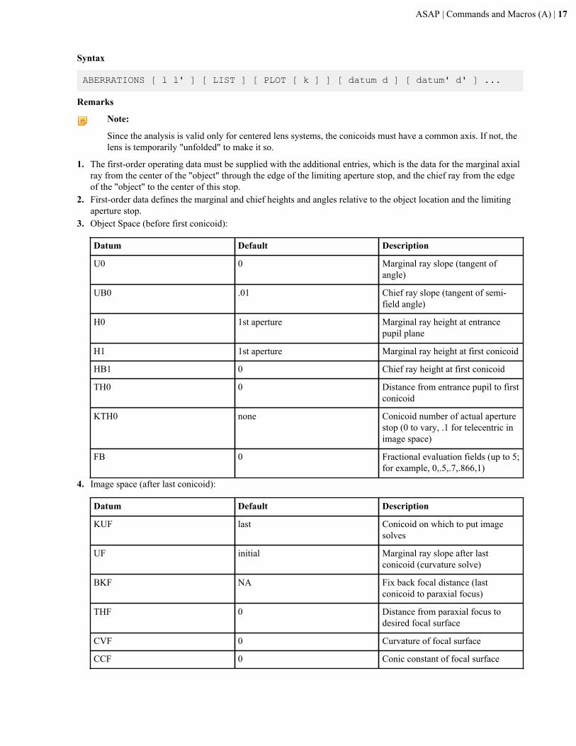
ASAP | Commands and Macros (A) | 17
Syntax
ABERRATIONS [ l l' ] [ LIST ] [ PLOT [ k ] ] [ datum d ] [ datum' d' ] ...
Remarks
Note:
Since the analysis is valid only for centered lens systems, the conicoids must have a common axis. If not, thelens is temporarily "unfolded" to make it so.
1. The first-order operating data must be supplied with the additional entries, which is the data for the marginal axialray from the center of the "object" through the edge of the limiting aperture stop, and the chief ray from the edgeof the "object" to the center of this stop.
2. First-order data defines the marginal and chief heights and angles relative to the object location and the limitingaperture stop.
3. Object Space (before first conicoid):
Datum Default Description
U0 0 Marginal ray slope (tangent ofangle)
UB0 .01 Chief ray slope (tangent of semi-field angle)
H0 1st aperture Marginal ray height at entrancepupil plane
H1 1st aperture Marginal ray height at first conicoid
HB1 0 Chief ray height at first conicoid
TH0 0 Distance from entrance pupil to firstconicoid
KTH0 none Conicoid number of actual aperturestop (0 to vary, .1 for telecentric inimage space)
FB 0 Fractional evaluation fields (up to 5;for example, 0,.5,.7,.866,1)
4. Image space (after last conicoid):
Datum Default Description
KUF last Conicoid on which to put imagesolves
UF initial Marginal ray slope after lastconicoid (curvature solve)
BKF NA Fix back focal distance (lastconicoid to paraxial focus)
THF 0 Distance from paraxial focus todesired focal surface
CVF 0 Curvature of focal surface
CCF 0 Conic constant of focal surface
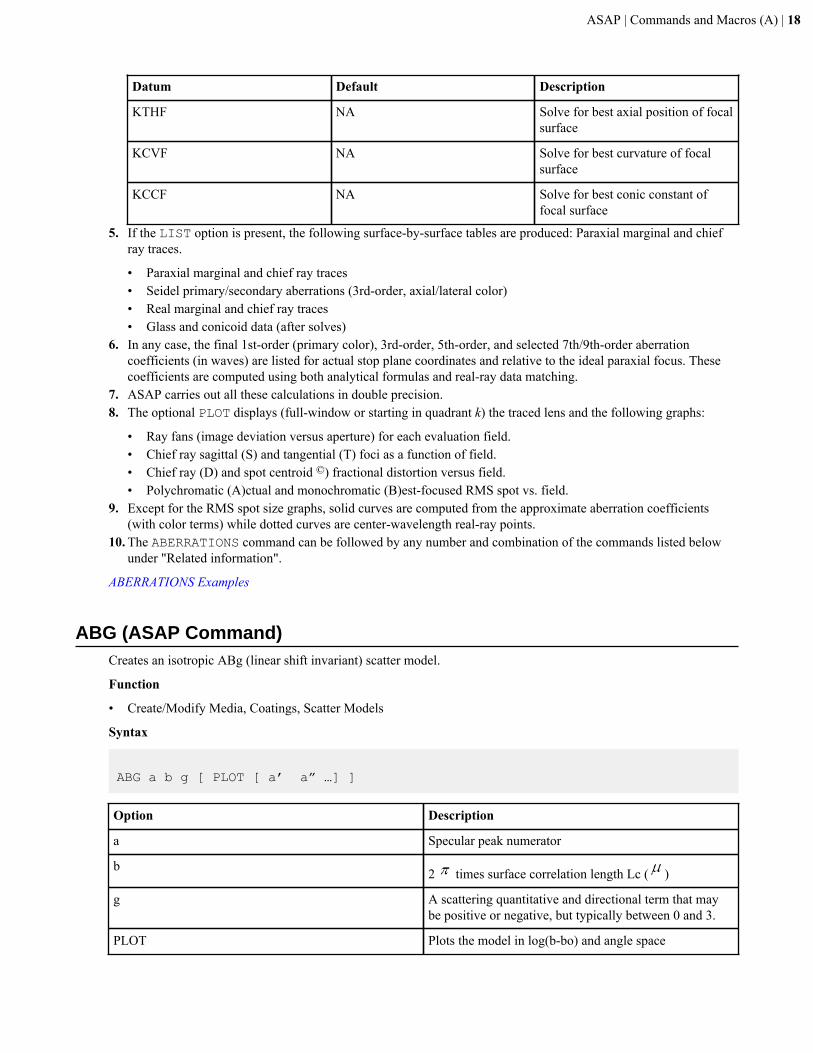
ASAP | Commands and Macros (A) | 18
Datum Default Description
KTHF NA Solve for best axial position of focalsurface
KCVF NA Solve for best curvature of focalsurface
KCCF NA Solve for best conic constant offocal surface
5. If the LIST option is present, the following surface-by-surface tables are produced: Paraxial marginal and chiefray traces.
• Paraxial marginal and chief ray traces• Seidel primary/secondary aberrations (3rd-order, axial/lateral color)• Real marginal and chief ray traces• Glass and conicoid data (after solves)
6. In any case, the final 1st-order (primary color), 3rd-order, 5th-order, and selected 7th/9th-order aberrationcoefficients (in waves) are listed for actual stop plane coordinates and relative to the ideal paraxial focus. Thesecoefficients are computed using both analytical formulas and real-ray data matching.
7. ASAP carries out all these calculations in double precision.8. The optional PLOT displays (full-window or starting in quadrant k) the traced lens and the following graphs:
• Ray fans (image deviation versus aperture) for each evaluation field.• Chief ray sagittal (S) and tangential (T) foci as a function of field.• Chief ray (D) and spot centroid ©) fractional distortion versus field.• Polychromatic (A)ctual and monochromatic (B)est-focused RMS spot vs. field.
9. Except for the RMS spot size graphs, solid curves are computed from the approximate aberration coefficients(with color terms) while dotted curves are center-wavelength real-ray points.
10. The ABERRATIONS command can be followed by any number and combination of the commands listed belowunder "Related information".
ABERRATIONS Examples
ABG (ASAP Command)Creates an isotropic ABg (linear shift invariant) scatter model.
Function
• Create/Modify Media, Coatings, Scatter Models
Syntax
ABG a b g [ PLOT [ a’ a” …] ]
Option Description
a Specular peak numerator
b 2 times surface correlation length Lc ( )
g A scattering quantitative and directional term that maybe positive or negative, but typically between 0 and 3.
PLOT Plots the model in log(b-bo) and angle space
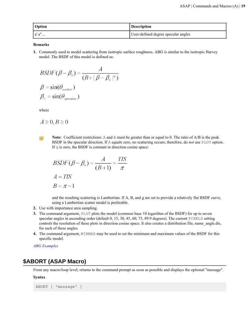
ASAP | Commands and Macros (A) | 19
Option Description
a' a"... User-defined degree specular angles
Remarks
1. Commonly used to model scattering from isotropic surface roughness. ABG is similar to the isotropic Harveymodel. The BSDF of this model is defined as:
where
Note: Coefficient restrictions: A and B must be greater than or equal to 0. The ratio of A/B is the peakBSDF in the specular direction. If A equals zero, no scattering occurs; therefore, do not use PLOT option.If g is zero, the BSDF is constant in direction cosine space:
and the resulting scattering is Lambertian. If A, B, and g are set to provide a relatively flat BSDF curve,using a Lambertian scatter model is preferable.
2. Use with importance area sampling.3. The command argument, PLOT plots the model (common base 10 logarithm of the BSDF) for up to seven
specular angles in ascending order (default 0, 15, 30, 45, 60, 75, 89.9 degrees). The current PIXELS settingcontrols the resolution of these plots in direction cosine space. It also creates a distribution file, name_angle.dis,for each of these angles.
4. The command argument, MINMAX may be used to set the minimum and maximum values of the BSDF for thisspecific model.
ABG Examples
$ABORT (ASAP Macro)From any macro/loop level, returns to the command prompt as soon as possible and displays the optional "message".
Syntax
ABORT [ 'message' ]

ASAP | Commands and Macros (A) | 20
Option Description
message Optional message to display
$ABORT Examples
ABSORB (ASAP Command Argument)Absorption or gain option, which is positive for an absorbing medium or negative for a gain (assigning) medium.
Syntax
... [ ABSORB a [ j q t ] ]
Option Description
a Volume absorption in inverse length units
j Its magnitude is the SURFACE designation for thisfunction when tracing a ray in this inhomogeneousmedium
t Step length
Remarks
1. If an absorption is not given (or zero), the program uses the wavelength and the imaginary part of the complexrefractive index (if specified) to calculate the absorption.
2. Inhomogeneous absorption or gain can be handled by assigning to the medium a GENERAL polynomial in theglobal coordinates X,Y,Z or USERFUNC function (with additional wavelength w dependence).
3. The magnitude of j is the SURFACE designation for this function.4. The absorption coefficient at each point in the medium is then given by:
5. The t is the step length to be used by the program when tracing a ray in this inhomogeneous medium.
ABSORB Examples
ACCURACY (ASAP Command)Provides user control of the trade-off between ray trace speed and accuracy when determining the ray/surfaceintersection.
Function
• Setup Trace
Syntax
ACCURACY [ HIGH | MEDIUM | LOW ] [ PARALLEL [ d ] ]
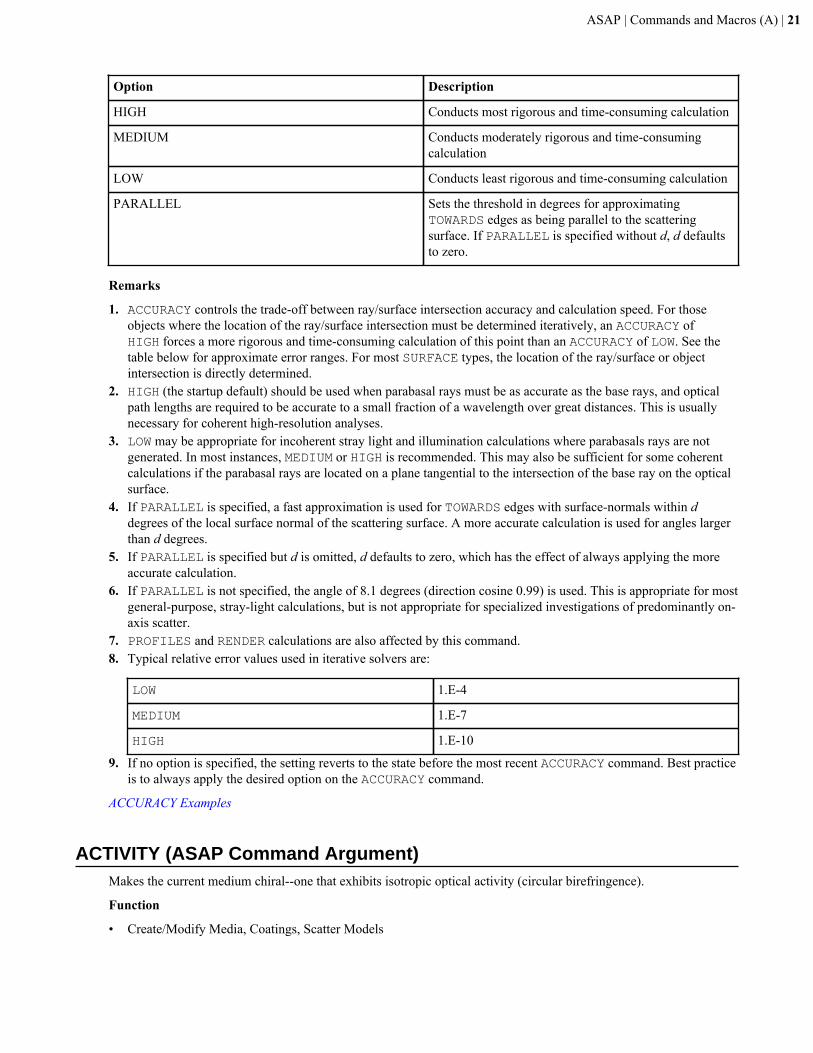
ASAP | Commands and Macros (A) | 21
Option Description
HIGH Conducts most rigorous and time-consuming calculation
MEDIUM Conducts moderately rigorous and time-consumingcalculation
LOW Conducts least rigorous and time-consuming calculation
PARALLEL Sets the threshold in degrees for approximatingTOWARDS edges as being parallel to the scatteringsurface. If PARALLEL is specified without d, d defaultsto zero.
Remarks
1. ACCURACY controls the trade-off between ray/surface intersection accuracy and calculation speed. For thoseobjects where the location of the ray/surface intersection must be determined iteratively, an ACCURACY ofHIGH forces a more rigorous and time-consuming calculation of this point than an ACCURACY of LOW. See thetable below for approximate error ranges. For most SURFACE types, the location of the ray/surface or objectintersection is directly determined.
2. HIGH (the startup default) should be used when parabasal rays must be as accurate as the base rays, and opticalpath lengths are required to be accurate to a small fraction of a wavelength over great distances. This is usuallynecessary for coherent high-resolution analyses.
3. LOW may be appropriate for incoherent stray light and illumination calculations where parabasals rays are notgenerated. In most instances, MEDIUM or HIGH is recommended. This may also be sufficient for some coherentcalculations if the parabasal rays are located on a plane tangential to the intersection of the base ray on the opticalsurface.
4. If PARALLEL is specified, a fast approximation is used for TOWARDS edges with surface-normals within ddegrees of the local surface normal of the scattering surface. A more accurate calculation is used for angles largerthan d degrees.
5. If PARALLEL is specified but d is omitted, d defaults to zero, which has the effect of always applying the moreaccurate calculation.
6. If PARALLEL is not specified, the angle of 8.1 degrees (direction cosine 0.99) is used. This is appropriate for mostgeneral-purpose, stray-light calculations, but is not appropriate for specialized investigations of predominantly on-axis scatter.
7. PROFILES and RENDER calculations are also affected by this command.8. Typical relative error values used in iterative solvers are:
LOW 1.E-4
MEDIUM 1.E-7
HIGH 1.E-10
9. If no option is specified, the setting reverts to the state before the most recent ACCURACY command. Best practiceis to always apply the desired option on the ACCURACY command.
ACCURACY Examples
ACTIVITY (ASAP Command Argument)Makes the current medium chiral--one that exhibits isotropic optical activity (circular birefringence).
Function
• Create/Modify Media, Coatings, Scatter Models
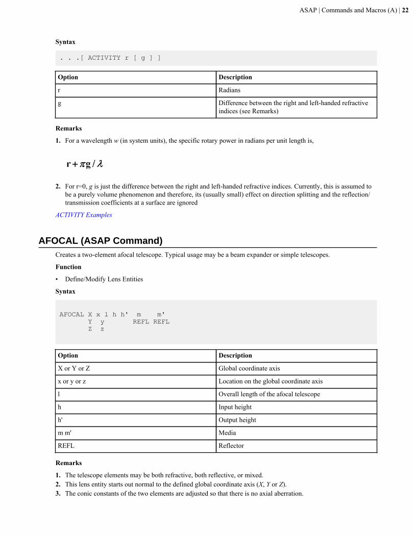
ASAP | Commands and Macros (A) | 22
Syntax
. . .[ ACTIVITY r [ g ] ]
Option Description
r Radians
g Difference between the right and left-handed refractiveindices (see Remarks)
Remarks
1. For a wavelength w (in system units), the specific rotary power in radians per unit length is,
2. For r=0, g is just the difference between the right and left-handed refractive indices. Currently, this is assumed to
be a purely volume phenomenon and therefore, its (usually small) effect on direction splitting and the reflection/transmission coefficients at a surface are ignored
ACTIVITY Examples
AFOCAL (ASAP Command)Creates a two-element afocal telescope. Typical usage may be a beam expander or simple telescopes.
Function
• Define/Modify Lens Entities
Syntax
AFOCAL X x l h h' m m' Y y REFL REFL Z z
Option Description
X or Y or Z Global coordinate axis
x or y or z Location on the global coordinate axis
l Overall length of the afocal telescope
h Input height
h' Output height
m m' Media
REFL Reflector
Remarks
1. The telescope elements may be both refractive, both reflective, or mixed.2. This lens entity starts out normal to the defined global coordinate axis (X, Y or Z).3. The conic constants of the two elements are adjusted so that there is no axial aberration.

ASAP | Commands and Macros (A) | 23
4. If h and h' are of opposite sign, there is an intermediate real focus.5. For a reflecting element, m should be -1 or REFL Either or both elements may be reflectors.
AFOCAL Examples
ALIGN (ASAP Command)Rotates object, entity, or source so that its direction vector is aligned to different specified direction.
Function
• Create/Modify Objects• Define/Modify Curvedge Entities• Define/Modify Lens Entities• Define/Modify Surfunc Entities• Modify Ray/Beam Data
Syntax
ALIGN a,b,c a',b',c' [ x,y,z ] [ LIST ]
Option Description
a, b, c First direction vector
a', b', c' Second direction vector
x, y, z Fixed point that the rotation axis passes through (defaultis the entity's reference point)
LIST Prints the resulting 4-by-4 transformation matrix
Remarks
1. ALIGN can be used when setting up systems for which you have only global vertex coordinates and global normalvectors. The rotation axis passes through the given point, and this point remains fixed during the transformation.Since it performs the most direct coordinate rotation, an ambiguous clocking rotation may occur. This commandrequires you to know the current direction vector as well as the desired orientation vector for each item.
2. Rotates object, entity, or source represented as a,b,c so that its direction vector is aligned to a different specifieddirection a', b', c.'
3. The rotation axis passes through a fixed point; that is, either point x,y,z or the entity's reference point (default).4. The LIST option causes the resulting 4-by-4 transformation matrix to be printed and decoded into simple
operations if possible.5. See the topic, General Input Techniques for various formats that are supported for the a, b, and c entries. For
instance, to align the average source direction with the positive Z axis direction, you can use the format, ALIGNDIR SOU 1 0 0 1. See the example.
6. Some commands, including SOURCE DIRECTION, require the specification of a direction vector. The followingformat can be used for this input entry.
Example
EMIT RECT Z 0 0 0 1LIST DIRSURFACE; PLANE Z 0ALIGN 0 0 1 DIR SOU 1PRINT
ALIGN Examples
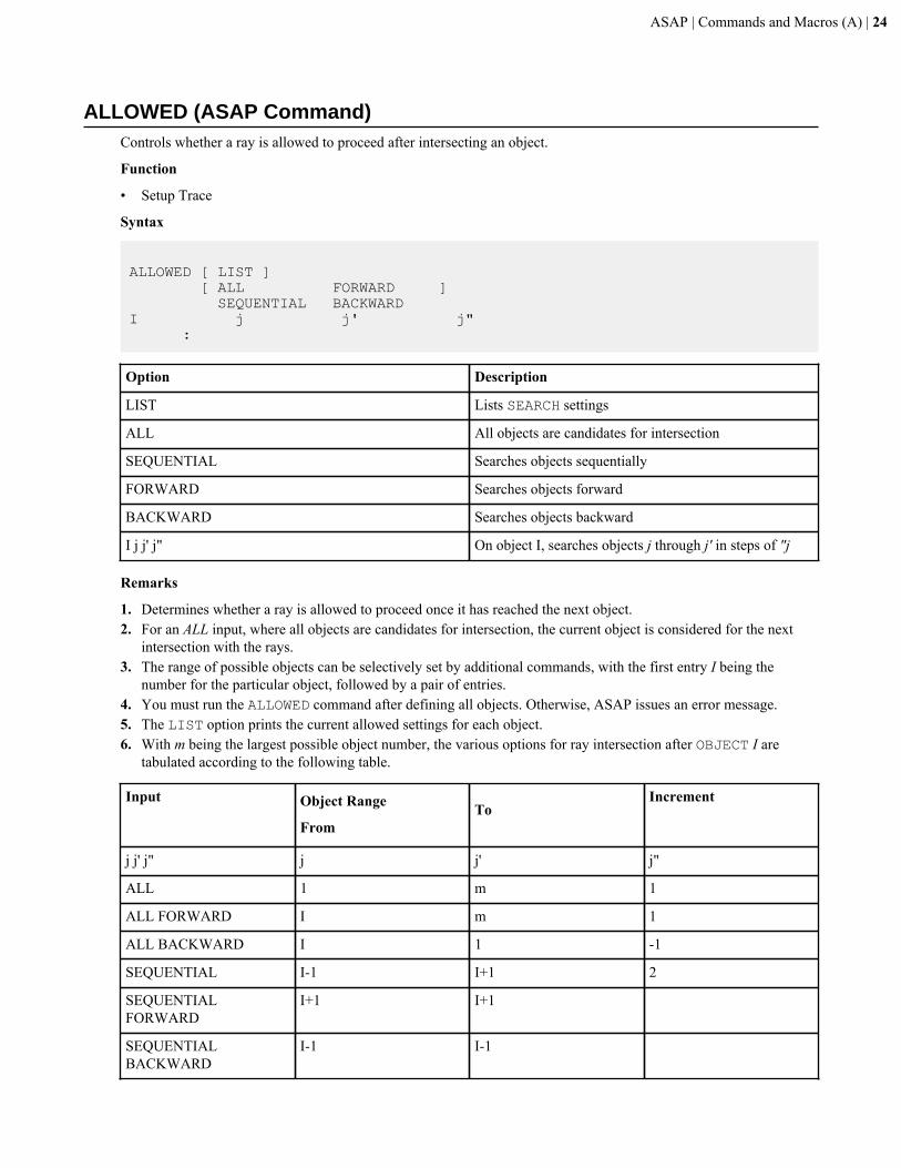
ASAP | Commands and Macros (A) | 24
ALLOWED (ASAP Command)Controls whether a ray is allowed to proceed after intersecting an object.
Function
• Setup Trace
Syntax
ALLOWED [ LIST ] [ ALL FORWARD ] SEQUENTIAL BACKWARDI j j' j" :
Option Description
LIST Lists SEARCH settings
ALL All objects are candidates for intersection
SEQUENTIAL Searches objects sequentially
FORWARD Searches objects forward
BACKWARD Searches objects backward
I j j' j" On object I, searches objects j through j' in steps of "j
Remarks
1. Determines whether a ray is allowed to proceed once it has reached the next object.2. For an ALL input, where all objects are candidates for intersection, the current object is considered for the next
intersection with the rays.3. The range of possible objects can be selectively set by additional commands, with the first entry I being the
number for the particular object, followed by a pair of entries.4. You must run the ALLOWED command after defining all objects. Otherwise, ASAP issues an error message.5. The LIST option prints the current allowed settings for each object.6. With m being the largest possible object number, the various options for ray intersection after OBJECT I are
tabulated according to the following table.
Input Object Range
FromTo
Increment
j j' j" j j' j"
ALL 1 m 1
ALL FORWARD I m 1
ALL BACKWARD I 1 -1
SEQUENTIAL I-1 I+1 2
SEQUENTIALFORWARD
I+1 I+1
SEQUENTIALBACKWARD
I-1 I-1
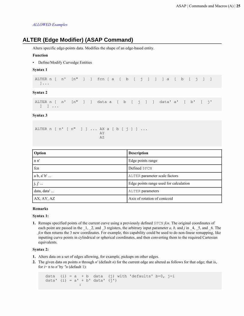
ASAP | Commands and Macros (A) | 25
ALLOWED Examples
ALTER (Edge Modifier) (ASAP Command)Alters specific edge-points data. Modifies the shape of an edge-based entity.
Function
• Define/Modify Curvedge Entities
Syntax 1
ALTER n [ n' [n" ] ] fcn [ a [ b [ j ] ] ] a [ b [ j ] ] ]...
Syntax 2
ALTER n [ n' [n" ] ] data a [ b [ j ] ] data' a' [ b' [ j' ] ] ...
Syntax 3
ALTER n [ n' [ n" ] ] ... AX a [ b [ j ] ] ... AY AZ
Option Description
n n' Edge points range
fcn Defined $FCN
a b, a' b' ... ALTER parameter scale factors
j, j' ... Edge points range used for calculation
data, data' ... ALTER parameters
AX, AY, AZ Axis of rotation of conicoid
Remarks
Syntax 1:
1. Remaps specified points of the current curve using a previously defined $FCN fcn. The original coordinates ofeach point are passed in the _1, _2, and _3 registers, the arbitrary input parameter a, b, and j in _4, _5, and _6. Thefcn then returns the 3 new coordinates. For example, this capability could be used to do non-linear remapping, likeinputting curve points in cylindrical or spherical coordinates, and then converting them to the required Cartesianequivalents.
Syntax 2:
1. Alters data on a set of edges allowing, for example, pickups on other edges.2. The given data on points n through n' (default n) for the current edge are altered as follows for that edge; that is,
for i= n to n' by "n (default 1):
data (i) = a + b data (j) with 'defaults' b=0, j=i data' (i) = a' + b' data' (j') :
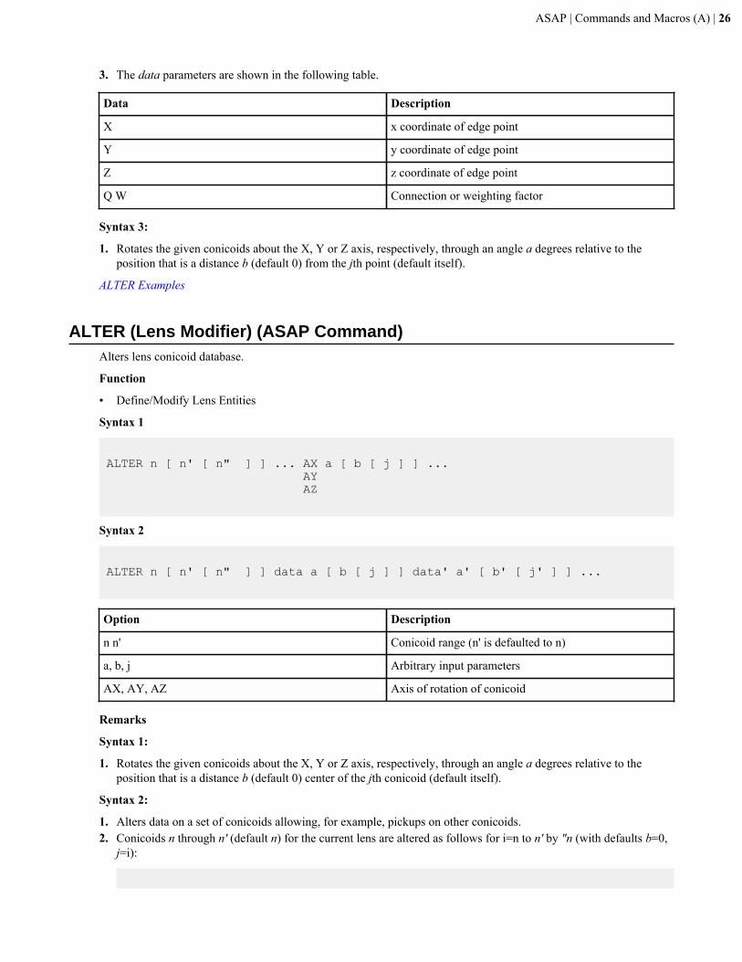
ASAP | Commands and Macros (A) | 26
3. The data parameters are shown in the following table.
Data Description
X x coordinate of edge point
Y y coordinate of edge point
Z z coordinate of edge point
Q W Connection or weighting factor
Syntax 3:
1. Rotates the given conicoids about the X, Y or Z axis, respectively, through an angle a degrees relative to theposition that is a distance b (default 0) from the jth point (default itself).
ALTER Examples
ALTER (Lens Modifier) (ASAP Command)Alters lens conicoid database.
Function
• Define/Modify Lens Entities
Syntax 1
ALTER n [ n' [ n" ] ] ... AX a [ b [ j ] ] ... AY AZ
Syntax 2
ALTER n [ n' [ n" ] ] data a [ b [ j ] ] data' a' [ b' [ j' ] ] ...
Option Description
n n' Conicoid range (n' is defaulted to n)
a, b, j Arbitrary input parameters
AX, AY, AZ Axis of rotation of conicoid
Remarks
Syntax 1:
1. Rotates the given conicoids about the X, Y or Z axis, respectively, through an angle a degrees relative to theposition that is a distance b (default 0) center of the jth conicoid (default itself).
Syntax 2:
1. Alters data on a set of conicoids allowing, for example, pickups on other conicoids.2. Conicoids n through n' (default n) for the current lens are altered as follows for i=n to n' by "n (with defaults b=0,
j=i):
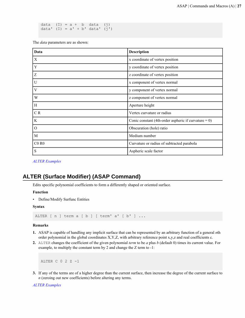
ASAP | Commands and Macros (A) | 27
data (I) = a + b data (j)data' (I) = a' + b' data' (j')
The data parameters are as shown:
Data Description
X x coordinate of vertex position
Y y coordinate of vertex position
Z z coordinate of vertex position
U x component of vertex normal
V y component of vertex normal
W z component of vertex normal
H Aperture height
C R Vertex curvature or radius
K Conic constant (4th-order aspheric if curvature = 0)
O Obscuration (hole) ratio
M Medium number
C0 R0 Curvature or radius of subtracted parabola
S Aspheric scale factor
ALTER Examples
ALTER (Surface Modifier) (ASAP Command)Edits specific polynomial coefficients to form a differently shaped or oriented surface.
Function
• Define/Modify Surfunc Entities
Syntax
ALTER [ n ] term a [ b ] [ term' a' [ b' ] ...
Remarks
1. ASAP is capable of handling any implicit surface that can be represented by an arbitrary function of a general nthorder polynomial in the global coordinates X,Y,Z, with arbitrary reference point x,y,z and real coefficients c.
2. ALTER changes the coefficient of the given polynomial term to be a plus b (default 0) times its current value. Forexample, to multiply the constant term by 2 and change the Z term to -1:
ALTER C 0 2 Z -1
3. If any of the terms are of a higher degree than the current surface, then increase the degree of the current surface ton (zeroing out new coefficients) before altering any terms.
ALTER Examples
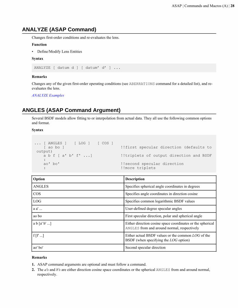
ASAP | Commands and Macros (A) | 28
ANALYZE (ASAP Command)Changes first-order conditions and re-evaluates the lens.
Function
• Define/Modify Lens Entities
Syntax
ANALYZE [ datum d ] [ datum’ d’ ] ...
Remarks
Changes any of the given first-order operating conditions (see ABERRATIONS command for a detailed list), and re-evaluates the lens.
ANALYZE Examples
ANGLES (ASAP Command Argument)Several BSDF models allow fitting to or interpolation from actual data. They all use the following common optionsand format.
Syntax
... [ ANGLES ] [ LOG ] [ COS ] [ ao bo ] !!first specular direction (defaults to output) a b f [ a' b' f' ...] !!triplets of output direction and BSDF : ao' bo' !!second specular direction : !!more triplets
Option Description
ANGLES Specifies spherical angle coordinates in degrees
COS Specifies angle coordinates in direction cosine
LOG Specifies common logarithmic BSDF values
a a' ... User-defined degree specular angles
ao bo First specular direction, polar and spherical angle
a b [a' b' ...] Either direction cosine space coordinates or the sphericalANGLES from and around normal, respectively
f [f' ...] Either actual BSDF values or the common LOG of theBSDF (when specifying the LOG option)
ao' bo' Second specular direction
Remarks
1. ASAP command arguments are optional and must follow a command.2. The a's and b's are either direction cosine space coordinates or the spherical ANGLES from and around normal,
respectively.
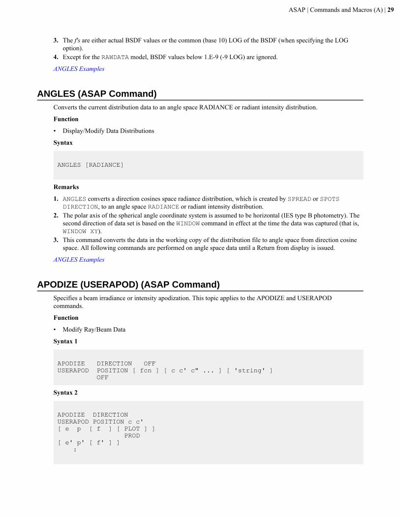
ASAP | Commands and Macros (A) | 29
3. The f's are either actual BSDF values or the common (base 10) LOG of the BSDF (when specifying the LOGoption).
4. Except for the RAWDATA model, BSDF values below 1.E-9 (-9 LOG) are ignored.
ANGLES Examples
ANGLES (ASAP Command)Converts the current distribution data to an angle space RADIANCE or radiant intensity distribution.
Function
• Display/Modify Data Distributions
Syntax
ANGLES [RADIANCE]
Remarks
1. ANGLES converts a direction cosines space radiance distribution, which is created by SPREAD or SPOTSDIRECTION, to an angle space RADIANCE or radiant intensity distribution.
2. The polar axis of the spherical angle coordinate system is assumed to be horizontal (IES type B photometry). Thesecond direction of data set is based on the WINDOW command in effect at the time the data was captured (that is,WINDOW XY).
3. This command converts the data in the working copy of the distribution file to angle space from direction cosinespace. All following commands are performed on angle space data until a Return from display is issued.
ANGLES Examples
APODIZE (USERAPOD) (ASAP Command)Specifies a beam irradiance or intensity apodization. This topic applies to the APODIZE and USERAPODcommands.
Function
• Modify Ray/Beam Data
Syntax 1
APODIZE DIRECTION OFFUSERAPOD POSITION [ fcn ] [ c c' c" ... ] [ 'string' ] OFF
Syntax 2
APODIZE DIRECTIONUSERAPOD POSITION c c'[ e p [ f ] [ PLOT ] ] PROD[ e' p' [ f' ] ] :
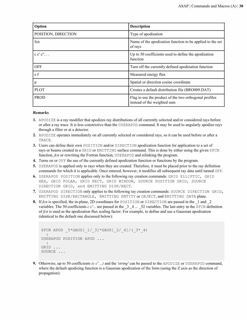
ASAP | Commands and Macros (A) | 30
Option Description
POSITION, DIRECTION Type of apodization
fcn Name of the apodization function to be applied to the setof rays
c c' c". . . Up to 50 coefficients used to define the apodizationfunction
OFF Turn off the currently defined apodization function
e f Measured energy flux
p Spatial or direction cosine coordinate
PLOT Creates a default distribution file (BRO009.DAT)
PROD Flag to use the product of the two orthogonal profilesinstead of the weighted sum
Remarks
1. APODIZE is a ray modifier that apodizes ray distributions of all currently selected and/or considered rays beforeor after a ray trace. It is less constrictive than the USERAPOD command. It may be used to angularly apodize raysthrough a filter or at a detector.
2. APODIZE operates immediately on all currently selected or considered rays, so it can be used before or after aTRACE.
3. Users can define their own POSITION and/or DIRECTION apodization function for application to a set ofrays or beams created in a GRID or EMITTING surface command. This is done by either using the given $FCNfunction, fcn or rewriting the Fortran function, USERAPOD and relinking the program.
4. Turns on or OFF the use of the currently defined apodization function or functions by the program.5. USERAPOD is applied only to rays when they are created. Therefore, it must be placed prior to the ray definition
commands for which it is applicable. Once entered, however, it modifies all subsequent ray data until turned OFF.6. USERAPOD POSITION applies only to the following ray creation commands: GRID ELLIPTIC, GRID
HEX, GRID POLAR, GRID RECT, GRID WINDOW, SOURCE POSITION GRID, SOURCEDIRECTION GRID, and EMITTING DISK/RECT.
7. USERAPOD DIRECTION only applies to the following ray creation commands: SOURCE DIRECTION GRID,EMITTING DISK/RECTANGLE, EMITTING ENTITY or OBJECT, and EMITTING DATA plane.
8. If fcn is specified, the in-plane, 2D coordinaes for POSITION or DIRECTION are passed in the _1 and _2variables. The 50 coefficients c c'... are passed in the _3 _4 ... _52 variables. The last entry in the $FCN definitionof fcn is used as the apodization flux scaling factor. For example, to define and use a Gaussian apodization(identical to the default one discussed below):
$FCN APOD _5*GAUS[_1/_3]*GAUS[_2/_4]/(_3*_4) :USERAPOD POSITION APOD ... :GRID ...SOURCE ...
9. Otherwise, up to 50 coefficients (c c' ...) and the 'string' can be passed to the APODIZE or USERAPOD command,where the default apodizing function is a Gaussian apodization of the form (using the Z axis as the direction ofpropagation):
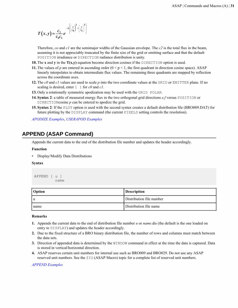
ASAP | Commands and Macros (A) | 31
Therefore, co and c1 are the semimajor widths of the Gaussian envelope. The c2 is the total flux in the beam,assuming it is not appreciably truncated by the finite size of the grid or emitting surface and that the defaultPOSITION irradiance or DIRECTION radiance distribution is unity.
10. The x and y in the T(x,y) equation become direction cosines if the DIRECTION option is used.11. The values of p are entered in ascending order (0 < p < 1, the first quadrant in direction cosine space). ASAP
linearly interpolates to obtain intermediate flux values. The remaining three quadrants are mapped by reflectionacross the coordinate axes.
12. The c0 and c1 values are used to scale p into the two coordinate values at the GRID or EMITTER plane. If noscaling is desired, enter 1 1 for c0 and c1.
13. Only a rotationally symmetric apodization may be used with the GRID POLAR.14. Syntax 2: a table of measured energy flux in the two orthogonal grid directions e,f versus POSITION or
DIRECTIONcosine p can be entered to apodize the grid.15. Syntax 2: If the PLOT option is used with the second syntax creates a default distribution file (BRO009.DAT) for
future plotting by the DISPLAY command (the current PIXELS setting controls the resolution).
APODIZE Examples, USERAPOD Examples
APPEND (ASAP Command)Appends the current data to the end of the distribution file number and updates the header accordingly.
Function
• Display/Modify Data Distributions
Syntax
APPEND [ u ] name
Option Description
u Distribution file number
name Distribution file name
Remarks
1. Appends the current data to the end of distribution file number u or name.dis (the default is the one loaded onentry to DISPLAY) and updates the header accordingly.
2. Due to the fixed structure of a BRO binary distribution file, the number of rows and columns must match betweenthe data sets.
3. Direction of appended data is determined by the WINDOW command in effect at the time the data is captured. Datais stored in vertical/horizontal direction.
4. ASAP reserves certain unit numbers for internal use such as BRO009 and BRO029. Do not use any ASAPreserved unit numbers. See the $IO (ASAP Macro) topic for a complete list of reserved unit numbers.
APPEND Examples
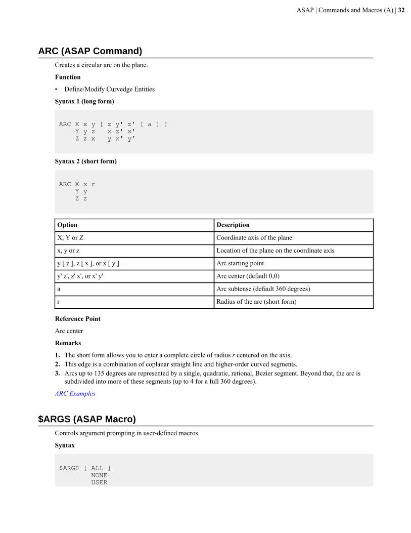
ASAP | Commands and Macros (A) | 32
ARC (ASAP Command)Creates a circular arc on the plane.
Function
• Define/Modify Curvedge Entities
Syntax 1 (long form)
ARC X x y [ z y' z' [ a ] ] Y y z x z' x' Z z x y x' y'
Syntax 2 (short form)
ARC X x r Y y Z z
Option Description
X, Y or Z Coordinate axis of the plane
x, y or z Location of the plane on the coordinate axis
y [ z ], z [ x ], or x [ y ] Arc starting point
y' z', z' x', or x' y' Arc center (default 0,0)
a Arc subtense (default 360 degrees)
r Radius of the arc (short form)
Reference Point
Arc center
Remarks
1. The short form allows you to enter a complete circle of radius r centered on the axis.2. This edge is a combination of coplanar straight line and higher-order curved segments.3. Arcs up to 135 degrees are represented by a single, quadratic, rational, Bezier segment. Beyond that, the arc is
subdivided into more of these segments (up to 4 for a full 360 degrees).
ARC Examples
$ARGS (ASAP Macro)Controls argument prompting in user-defined macros.
Syntax
$ARGS [ ALL ] NONE USER
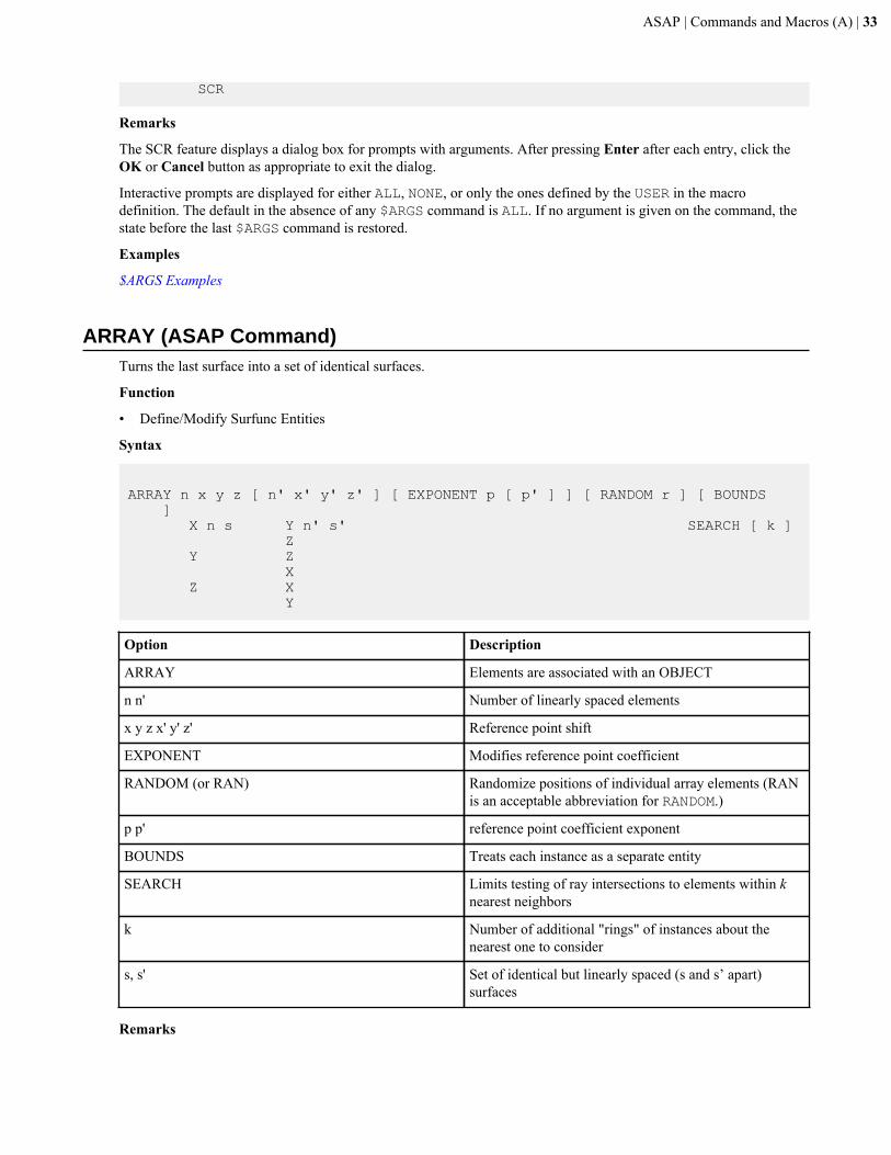
ASAP | Commands and Macros (A) | 33
SCR
Remarks
The SCR feature displays a dialog box for prompts with arguments. After pressing Enter after each entry, click theOK or Cancel button as appropriate to exit the dialog.
Interactive prompts are displayed for either ALL, NONE, or only the ones defined by the USER in the macrodefinition. The default in the absence of any $ARGS command is ALL. If no argument is given on the command, thestate before the last $ARGS command is restored.
Examples
$ARGS Examples
ARRAY (ASAP Command)Turns the last surface into a set of identical surfaces.
Function
• Define/Modify Surfunc Entities
Syntax
ARRAY n x y z [ n' x' y' z' ] [ EXPONENT p [ p' ] ] [ RANDOM r ] [ BOUNDS ] X n s Y n' s' SEARCH [ k ] Z Y Z X Z X Y
Option Description
ARRAY Elements are associated with an OBJECT
n n' Number of linearly spaced elements
x y z x' y' z' Reference point shift
EXPONENT Modifies reference point coefficient
RANDOM (or RAN) Randomize positions of individual array elements (RANis an acceptable abbreviation for RANDOM.)
p p' reference point coefficient exponent
BOUNDS Treats each instance as a separate entity
SEARCH Limits testing of ray intersections to elements within knearest neighbors
k Number of additional "rings" of instances about thenearest one to consider
s, s' Set of identical but linearly spaced (s and s’ apart)surfaces
Remarks

ASAP | Commands and Macros (A) | 34
1. Turns the last surface into an n+1 by n'+1 set of identical but linearly spaced (s and s' apart) surfaces. For the first,more general (possibly skew) syntax, the replicated surfaces are spaced according to the equation:
2. The EXPONENT option allows the reference point coefficient to be modified as follows:
3. The defaults for p and p' are both 1.4. Positions of each element of the array (except for the original one, i=0, j=0) can be RANDOMized a relative amount
given by the fractional part of r. The whole/integer part of r (default 0) determines a unique random sequence tobe used. See the topic, "Mathematical Functions Supported".
5. Each instance (that is, element) can be optionally treated as a separate entity on a BOUNDS command. Otherwise,if it is used as a base object surface, the SEARCH for any ray intersection is restricted to the instance nearest towhere the ray intersects the plane of the array (default is a k of zero). SEARCH cannot be applied to an ARRAYwith an ARRAY BOUNDS command.
6. The k option is the number of additional "rings" of instances about this nearest one to also consider. For largearrays, this can speed up the trace calculation by orders of magnitude, but runs the risk of some rays unphysicallymissing the object. Larger values of k reduce this risk but slow down the trace.
Note: From ASAP, open and run the sample project, backlight.apf, located in your <ASAP installfolder>\Projects\Samples\LCDbacklight.
Note: On the Quick Start toolbar in ASAP, click Interactive Scripts, Array Enhancers to view tools forcreating several forms of arrayed structures. If the toolbar is not visible, click View, Quick Start Bar.
ARRAY Examples
ARRAY NONLINEAR (ASAP Command)Turns the last surface into a set of identical but nonlinearly spaced surfaces.
Function
• Define/Modify Surface Entities
Syntax 1
ARRAY NONLINEAR v {f|TABLE|MVFCN|USERPROG} n v’ {f'|TABLE|MVFCN|USERPROG} n' [POSITION] [RANDOM r] [SEARCH k|BOUNDS]
Syntax 2
ARRAY NONLINEAR v {f|MVFCN|USERPROG} w v’ {f'|MVFCN|USERPROG} w' [WIDTH] [POSITION] [RANDOM r] [SEARCH k|BOUNDS]
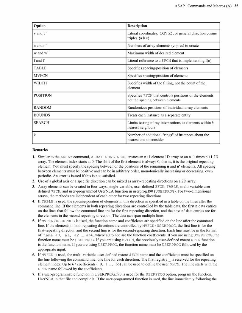
ASAP | Commands and Macros (A) | 35
Option Description
v and v’ Literal coordinates, {X|Y|Z}, or general direction cosinetriples {a b c}
n and n’ Numbers of array elements (copies) to create
w and w’ Maximum width of desired element
f and f’ Literal reference to a $FCN that is implementing f(n)
TABLE Specifies spacing/position of elements
MVFCN Specifies spacing/position of elements
WIDTH Specifies width of the filling, not the count of theelement
POSITION Specifies $FCN that controls positions of the elements,not the spacing between elements
RANDOM Randomizes positions of individual array elements
BOUNDS Treats each instance as a separate entity
SEARCH Limits testing of ray intersections to elements within knearest neighbors
k Number of additional "rings" of instances about thenearest one to consider
Remarks
1. Similar to the ARRAY command, ARRAY NONLINEAR creates an n+1 element 1D array or an n+1 times n'+1 2Darray. The element index starts at 0. The shift of the first element is always 0; that is, it is the original repeatingelement. You must specify the spacing between or the positions of the remaining n and n' elements. All spacingbetween elements must be positive and can be in arbitrary order, monotonically increasing or decreasing, evenperiodic. An error is issued if this is not satisfied.
2. Use of a global axis or a specific direction can be mixed as array-repeating directions on a 2D array.3. Array elements can be created in four ways: single-variable, user-defined $FCN, TABLE, multi-variable user-
defined $FCN, and user-programmed UserNLA function in userprog.f90 (USERPROG). For two-dimensionalarrays, the methods are independent of each other for two repeating directions.
4. If TABLE is used, the spacing/position of elements in this direction is specified in a table on the lines after thecommand line. If the elements in both repeating directions are controlled by the table data, the first n data entrieson the lines that follow the command line are for the first repeating direction, and the next n’ data entries are forthe elements in the second repeating direction. The data can span multiple lines.
5. If MVFCN/USERPROG is used, the function name and coefficients are specified on the line after the commandline. If the elements in both repeating directions are controlled by MVFCN/USERPROG, the first line is for thefirst-repeating direction and the second line is for the second-repeating direction. Each line must be in the formatof: name a0, a1, a2 … a66, where a0 to a66 are the function coefficients. If you are using USERPROG, thefunction name must be USERPROG. If you are using MVFCN, the previously user-defined macro $FCN functionis the function name. If you are using USERPROG, the function name must be USERPROG followed by theappropriate input.
6. If MVFCN is used, the multi-variable, user-defined macro $FCN name and the coefficients must be specified onthe line following the command line; one line for each direction. The first registry _ is reserved for the repeatingelement index. Up to 67 coefficients (_0, _1 ..., _66) can be used to define the user $FCN. The line starts with the$FCN name followed by the coefficients.
7. If a user-programmable function in USERPROG.f90 is used for the USERPROG option, program the function,UserNLA in that file and compile it. If the user-programmed function is used, the line immediately following the
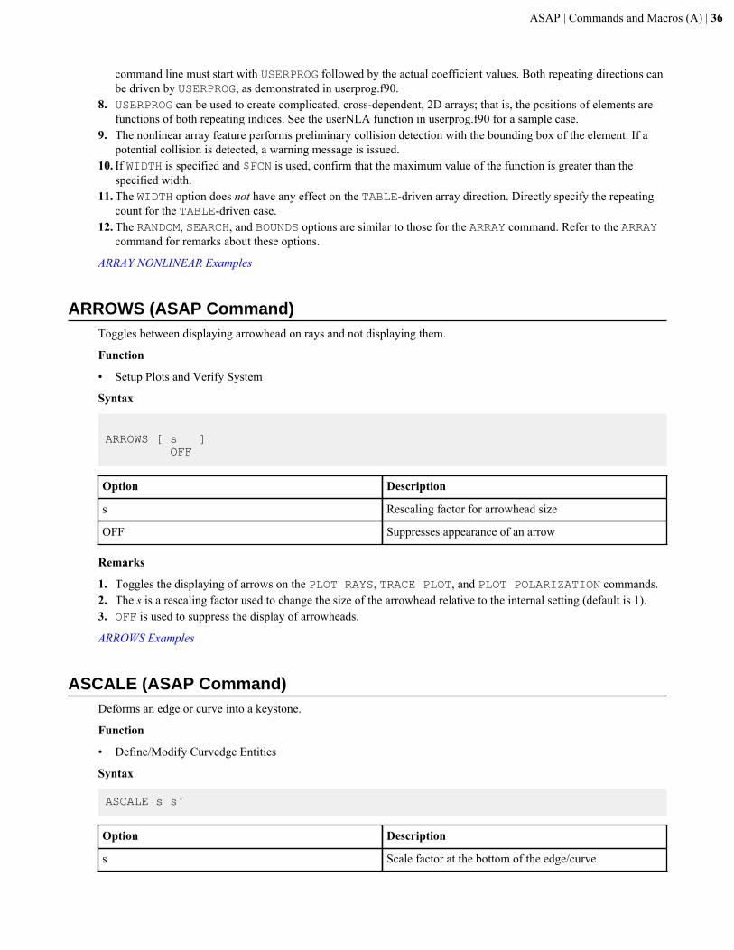
ASAP | Commands and Macros (A) | 36
command line must start with USERPROG followed by the actual coefficient values. Both repeating directions canbe driven by USERPROG, as demonstrated in userprog.f90.
8. USERPROG can be used to create complicated, cross-dependent, 2D arrays; that is, the positions of elements arefunctions of both repeating indices. See the userNLA function in userprog.f90 for a sample case.
9. The nonlinear array feature performs preliminary collision detection with the bounding box of the element. If apotential collision is detected, a warning message is issued.
10. If WIDTH is specified and $FCN is used, confirm that the maximum value of the function is greater than thespecified width.
11. The WIDTH option does not have any effect on the TABLE-driven array direction. Directly specify the repeatingcount for the TABLE-driven case.
12. The RANDOM, SEARCH, and BOUNDS options are similar to those for the ARRAY command. Refer to the ARRAYcommand for remarks about these options.
ARRAY NONLINEAR Examples
ARROWS (ASAP Command)Toggles between displaying arrowhead on rays and not displaying them.
Function
• Setup Plots and Verify System
Syntax
ARROWS [ s ] OFF
Option Description
s Rescaling factor for arrowhead size
OFF Suppresses appearance of an arrow
Remarks
1. Toggles the displaying of arrows on the PLOT RAYS, TRACE PLOT, and PLOT POLARIZATION commands.2. The s is a rescaling factor used to change the size of the arrowhead relative to the internal setting (default is 1).3. OFF is used to suppress the display of arrowheads.
ARROWS Examples
ASCALE (ASAP Command)Deforms an edge or curve into a keystone.
Function
• Define/Modify Curvedge Entities
Syntax
ASCALE s s'
Option Description
s Scale factor at the bottom of the edge/curve
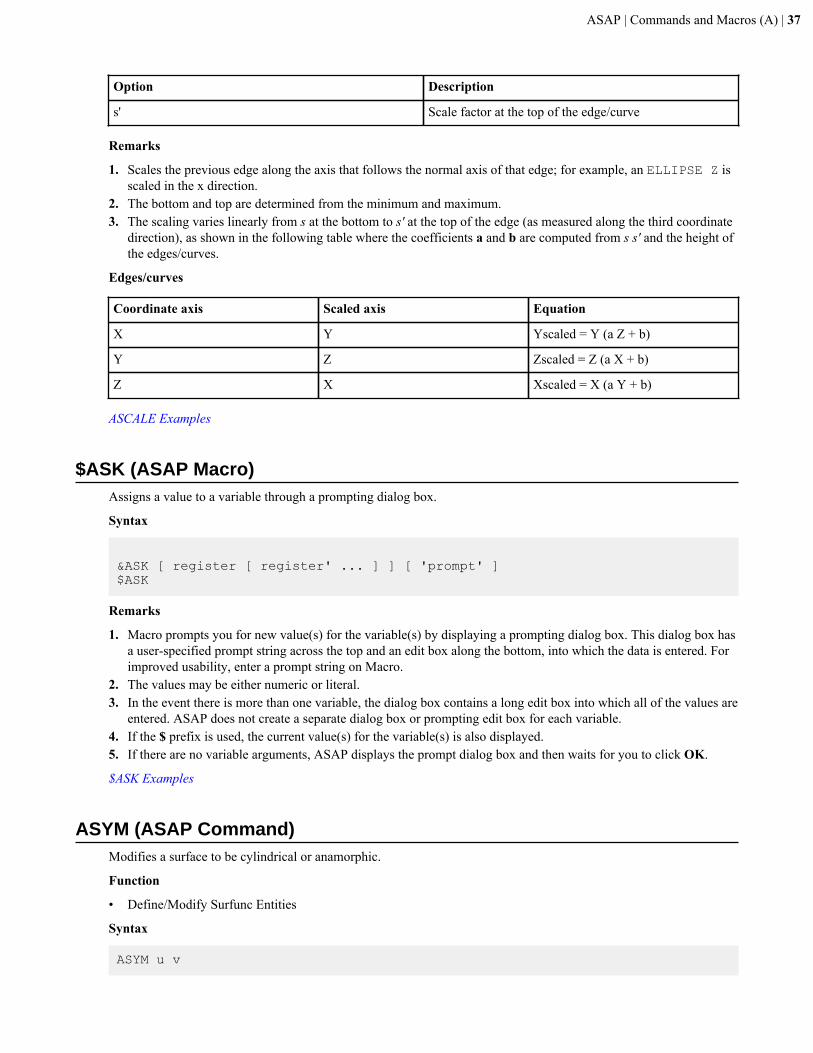
ASAP | Commands and Macros (A) | 37
Option Description
s' Scale factor at the top of the edge/curve
Remarks
1. Scales the previous edge along the axis that follows the normal axis of that edge; for example, an ELLIPSE Z isscaled in the x direction.
2. The bottom and top are determined from the minimum and maximum.3. The scaling varies linearly from s at the bottom to s' at the top of the edge (as measured along the third coordinate
direction), as shown in the following table where the coefficients a and b are computed from s s' and the height ofthe edges/curves.
Edges/curves
Coordinate axis Scaled axis Equation
X Y Yscaled = Y (a Z + b)
Y Z Zscaled = Z (a X + b)
Z X Xscaled = X (a Y + b)
ASCALE Examples
$ASK (ASAP Macro)Assigns a value to a variable through a prompting dialog box.
Syntax
&ASK [ register [ register' ... ] ] [ 'prompt' ]$ASK
Remarks
1. Macro prompts you for new value(s) for the variable(s) by displaying a prompting dialog box. This dialog box hasa user-specified prompt string across the top and an edit box along the bottom, into which the data is entered. Forimproved usability, enter a prompt string on Macro.
2. The values may be either numeric or literal.3. In the event there is more than one variable, the dialog box contains a long edit box into which all of the values are
entered. ASAP does not create a separate dialog box or prompting edit box for each variable.4. If the $ prefix is used, the current value(s) for the variable(s) is also displayed.5. If there are no variable arguments, ASAP displays the prompt dialog box and then waits for you to click OK.
$ASK Examples
ASYM (ASAP Command)Modifies a surface to be cylindrical or anamorphic.
Function
• Define/Modify Surfunc Entities
Syntax
ASYM u v
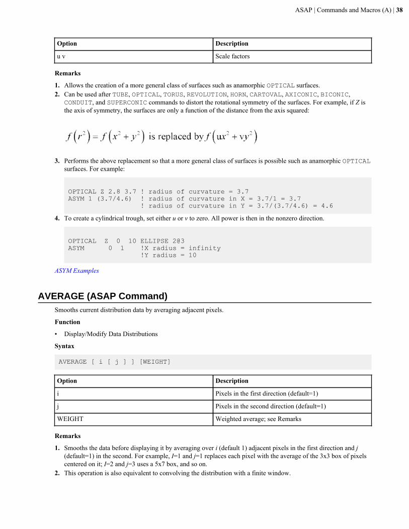
ASAP | Commands and Macros (A) | 38
Option Description
u v Scale factors
Remarks
1. Allows the creation of a more general class of surfaces such as anamorphic OPTICAL surfaces.2. Can be used after TUBE, OPTICAL, TORUS, REVOLUTION, HORN, CARTOVAL, AXICONIC, BICONIC,
CONDUIT, and SUPERCONIC commands to distort the rotational symmetry of the surfaces. For example, if Z isthe axis of symmetry, the surfaces are only a function of the distance from the axis squared:
3. Performs the above replacement so that a more general class of surfaces is possible such as anamorphic OPTICAL
surfaces. For example:
OPTICAL Z 2.8 3.7 ! radius of curvature = 3.7ASYM 1 (3.7/4.6) ! radius of curvature in X = 3.7/1 = 3.7 ! radius of curvature in Y = 3.7/(3.7/4.6) = 4.6
4. To create a cylindrical trough, set either u or v to zero. All power is then in the nonzero direction.
OPTICAL Z 0 10 ELLIPSE 2@3ASYM 0 1 !X radius = infinity !Y radius = 10
ASYM Examples
AVERAGE (ASAP Command)Smooths current distribution data by averaging adjacent pixels.
Function
• Display/Modify Data Distributions
Syntax
AVERAGE [ i [ j ] ] [WEIGHT]
Option Description
i Pixels in the first direction (default=1)
j Pixels in the second direction (default=1)
WEIGHT Weighted average; see Remarks
Remarks
1. Smooths the data before displaying it by averaging over i (default 1) adjacent pixels in the first direction and j(default=1) in the second. For example, I=1 and j=1 replaces each pixel with the average of the 3x3 box of pixelscentered on it; I=2 and j=3 uses a 5x7 box, and so on.
2. This operation is also equivalent to convolving the distribution with a finite window.
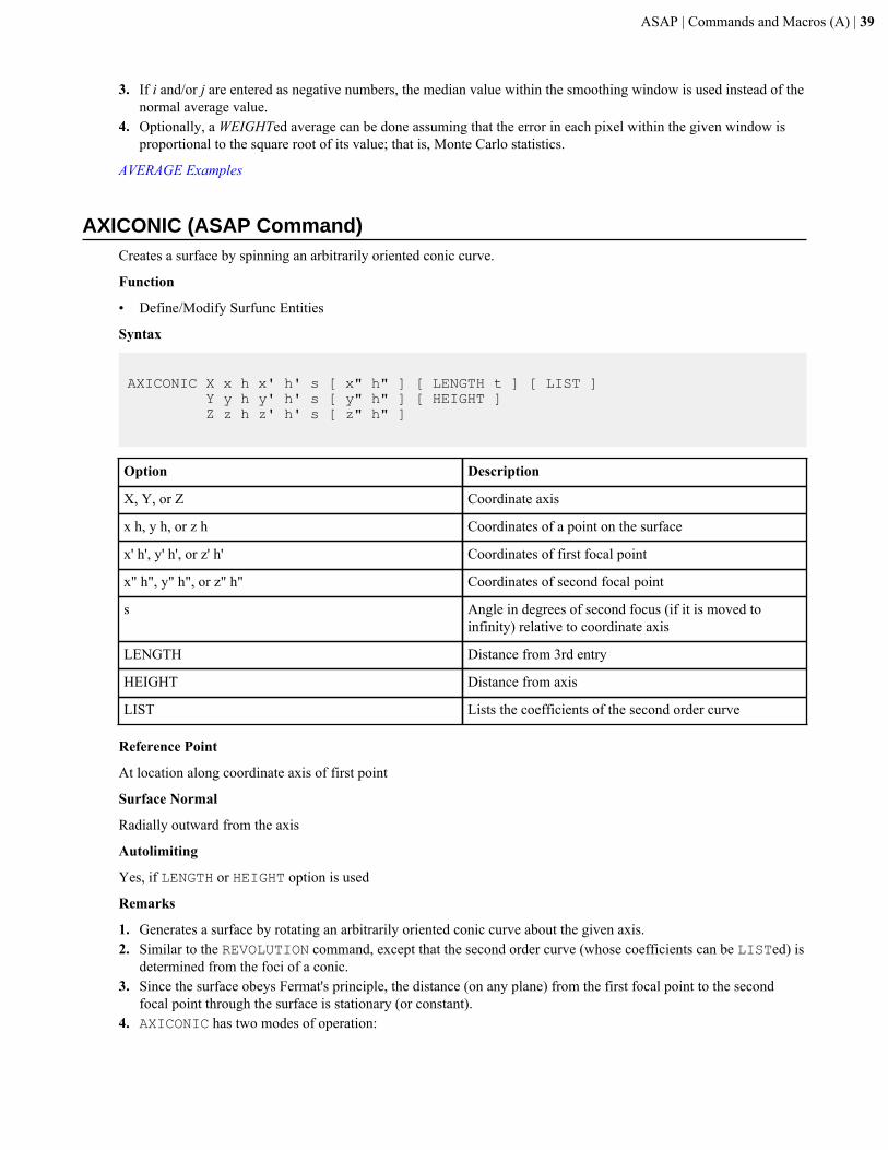
ASAP | Commands and Macros (A) | 39
3. If i and/or j are entered as negative numbers, the median value within the smoothing window is used instead of thenormal average value.
4. Optionally, a WEIGHTed average can be done assuming that the error in each pixel within the given window isproportional to the square root of its value; that is, Monte Carlo statistics.
AVERAGE Examples
AXICONIC (ASAP Command)Creates a surface by spinning an arbitrarily oriented conic curve.
Function
• Define/Modify Surfunc Entities
Syntax
AXICONIC X x h x' h' s [ x" h" ] [ LENGTH t ] [ LIST ] Y y h y' h' s [ y" h" ] [ HEIGHT ] Z z h z' h' s [ z" h" ]
Option Description
X, Y, or Z Coordinate axis
x h, y h, or z h Coordinates of a point on the surface
x' h', y' h', or z' h' Coordinates of first focal point
x" h", y" h", or z" h" Coordinates of second focal point
s Angle in degrees of second focus (if it is moved toinfinity) relative to coordinate axis
LENGTH Distance from 3rd entry
HEIGHT Distance from axis
LIST Lists the coefficients of the second order curve
Reference Point
At location along coordinate axis of first point
Surface Normal
Radially outward from the axis
Autolimiting
Yes, if LENGTH or HEIGHT option is used
Remarks
1. Generates a surface by rotating an arbitrarily oriented conic curve about the given axis.2. Similar to the REVOLUTION command, except that the second order curve (whose coefficients can be LISTed) is
determined from the foci of a conic.3. Since the surface obeys Fermat's principle, the distance (on any plane) from the first focal point to the second
focal point through the surface is stationary (or constant).4. AXICONIC has two modes of operation:
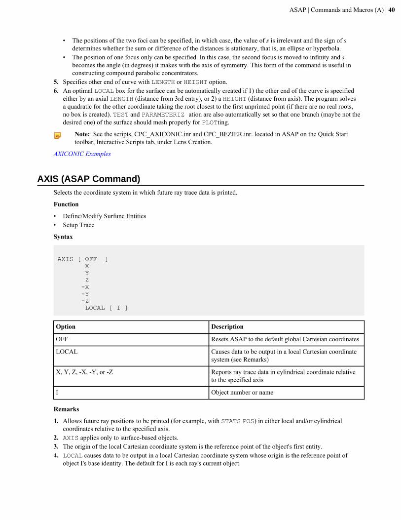
ASAP | Commands and Macros (A) | 40
• The positions of the two foci can be specified, in which case, the value of s is irrelevant and the sign of sdetermines whether the sum or difference of the distances is stationary, that is, an ellipse or hyperbola.
• The position of one focus only can be specified. In this case, the second focus is moved to infinity and sbecomes the angle (in degrees) it makes with the axis of symmetry. This form of the command is useful inconstructing compound parabolic concentrators.
5. Specifies other end of curve with LENGTH or HEIGHT option.6. An optimal LOCAL box for the surface can be automatically created if 1) the other end of the curve is specified
either by an axial LENGTH (distance from 3rd entry), or 2) a HEIGHT (distance from axis). The program solvesa quadratic for the other coordinate taking the root closest to the first unprimed point (if there are no real roots,no box is created). TEST and PARAMETERIZ ation are also automatically set so that one branch (maybe not thedesired one) of the surface should mesh properly for PLOTting.
Note: See the scripts, CPC_AXICONIC.inr and CPC_BEZIER.inr. located in ASAP on the Quick Starttoolbar, Interactive Scripts tab, under Lens Creation.
AXICONIC Examples
AXIS (ASAP Command)Selects the coordinate system in which future ray trace data is printed.
Function
• Define/Modify Surfunc Entities• Setup Trace
Syntax
AXIS [ OFF ] X Y Z -X -Y -Z LOCAL [ I ]
Option Description
OFF Resets ASAP to the default global Cartesian coordinates
LOCAL Causes data to be output in a local Cartesian coordinatesystem (see Remarks)
X, Y, Z, -X, -Y, or -Z Reports ray trace data in cylindrical coordinate relativeto the specified axis
I Object number or name
Remarks
1. Allows future ray positions to be printed (for example, with STATS POS) in either local and/or cylindricalcoordinates relative to the specified axis.
2. AXIS applies only to surface-based objects.3. The origin of the local Cartesian coordinate system is the reference point of the object's first entity.4. LOCAL causes data to be output in a local Cartesian coordinate system whose origin is the reference point of
object I's base identity. The default for I is each ray's current object.
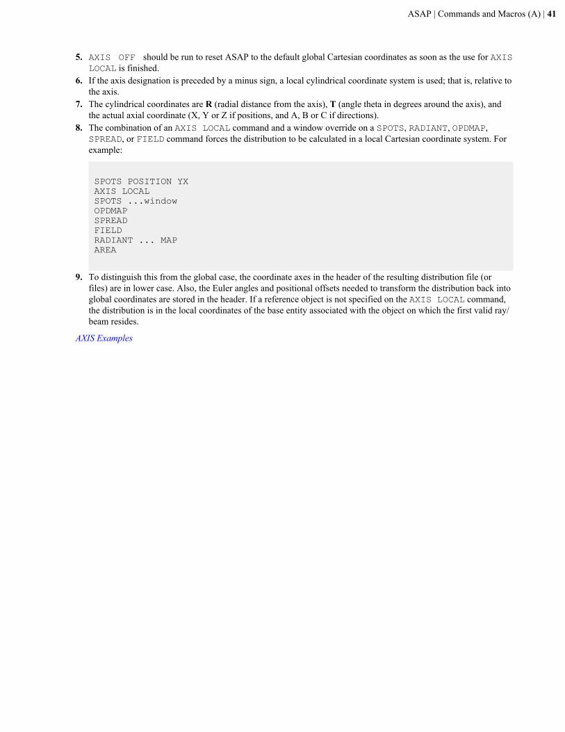
ASAP | Commands and Macros (A) | 41
5. AXIS OFF should be run to reset ASAP to the default global Cartesian coordinates as soon as the use for AXISLOCAL is finished.
6. If the axis designation is preceded by a minus sign, a local cylindrical coordinate system is used; that is, relative tothe axis.
7. The cylindrical coordinates are R (radial distance from the axis), T (angle theta in degrees around the axis), andthe actual axial coordinate (X, Y or Z if positions, and A, B or C if directions).
8. The combination of an AXIS LOCAL command and a window override on a SPOTS, RADIANT, OPDMAP,SPREAD, or FIELD command forces the distribution to be calculated in a local Cartesian coordinate system. Forexample:
SPOTS POSITION YXAXIS LOCALSPOTS ...windowOPDMAPSPREADFIELDRADIANT ... MAPAREA
9. To distinguish this from the global case, the coordinate axes in the header of the resulting distribution file (orfiles) are in lower case. Also, the Euler angles and positional offsets needed to transform the distribution back intoglobal coordinates are stored in the header. If a reference object is not specified on the AXIS LOCAL command,the distribution is in the local coordinates of the base entity associated with the object on which the first valid ray/beam resides.
AXIS Examples
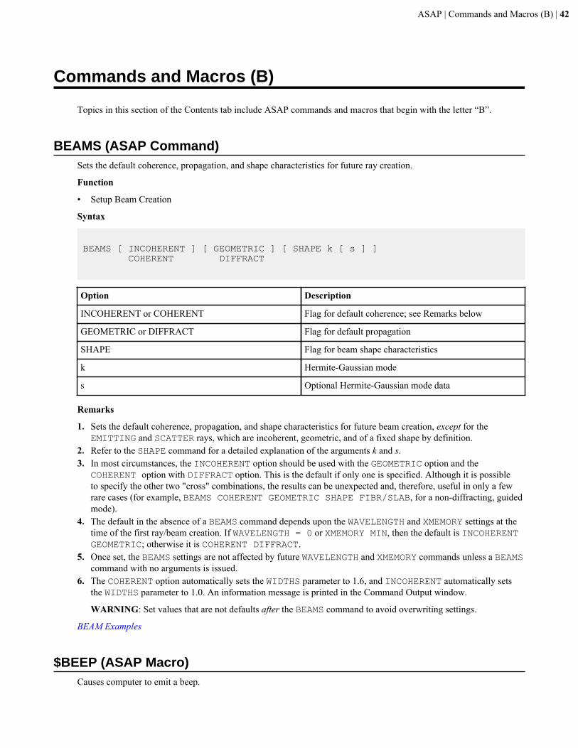
ASAP | Commands and Macros (B) | 42
Commands and Macros (B)
Topics in this section of the Contents tab include ASAP commands and macros that begin with the letter “B”.
BEAMS (ASAP Command)Sets the default coherence, propagation, and shape characteristics for future ray creation.
Function
• Setup Beam Creation
Syntax
BEAMS [ INCOHERENT ] [ GEOMETRIC ] [ SHAPE k [ s ] ] COHERENT DIFFRACT
Option Description
INCOHERENT or COHERENT Flag for default coherence; see Remarks below
GEOMETRIC or DIFFRACT Flag for default propagation
SHAPE Flag for beam shape characteristics
k Hermite-Gaussian mode
s Optional Hermite-Gaussian mode data
Remarks
1. Sets the default coherence, propagation, and shape characteristics for future beam creation, except for theEMITTING and SCATTER rays, which are incoherent, geometric, and of a fixed shape by definition.
2. Refer to the SHAPE command for a detailed explanation of the arguments k and s.3. In most circumstances, the INCOHERENT option should be used with the GEOMETRIC option and the
COHERENT option with DIFFRACT option. This is the default if only one is specified. Although it is possibleto specify the other two "cross" combinations, the results can be unexpected and, therefore, useful in only a fewrare cases (for example, BEAMS COHERENT GEOMETRIC SHAPE FIBR/SLAB, for a non-diffracting, guidedmode).
4. The default in the absence of a BEAMS command depends upon the WAVELENGTH and XMEMORY settings at thetime of the first ray/beam creation. If WAVELENGTH = 0 or XMEMORY MIN, then the default is INCOHERENTGEOMETRIC; otherwise it is COHERENT DIFFRACT.
5. Once set, the BEAMS settings are not affected by future WAVELENGTH and XMEMORY commands unless a BEAMScommand with no arguments is issued.
6. The COHERENT option automatically sets the WIDTHS parameter to 1.6, and INCOHERENT automatically setsthe WIDTHS parameter to 1.0. An information message is printed in the Command Output window.
WARNING: Set values that are not defaults after the BEAMS command to avoid overwriting settings.
BEAM Examples
$BEEP (ASAP Macro)Causes computer to emit a beep.

ASAP | Commands and Macros (B) | 43
Syntax
$BEEP [ n [ s ] ]
Remarks
Causes the terminal or console to beep n times (default 1) with s seconds (default 0.00) between each beep.
$BEEP Examples
BEND (ASAP Command)Bends the last surface along a parabolic curve.
Function
• Define/Modify Surfunc Entities
Syntax
BEND X c [ c' ] Y Z
Option Description
X Y or Z Axis which is bent
c c' Curvature coefficients of the bending
Remarks
1. Bends the surface (relative to its reference point) by replacing the given coordinate in its polynomial function witha quadratic in the other two coordinates, for example, for a BEND Z:
2. The c coefficients are the curvatures (inverse radii) of the bending.
Note: This operation may double the order of the polynomial.
BEND Examples
BEZIER (ASAP Command)Creates a Bezier edge/curve in the plane.
Function
• Define/Modify Curvedge Entities
Syntax
BEZIER X x y y' c [ c' [ c" ... ] ] Y y z z'
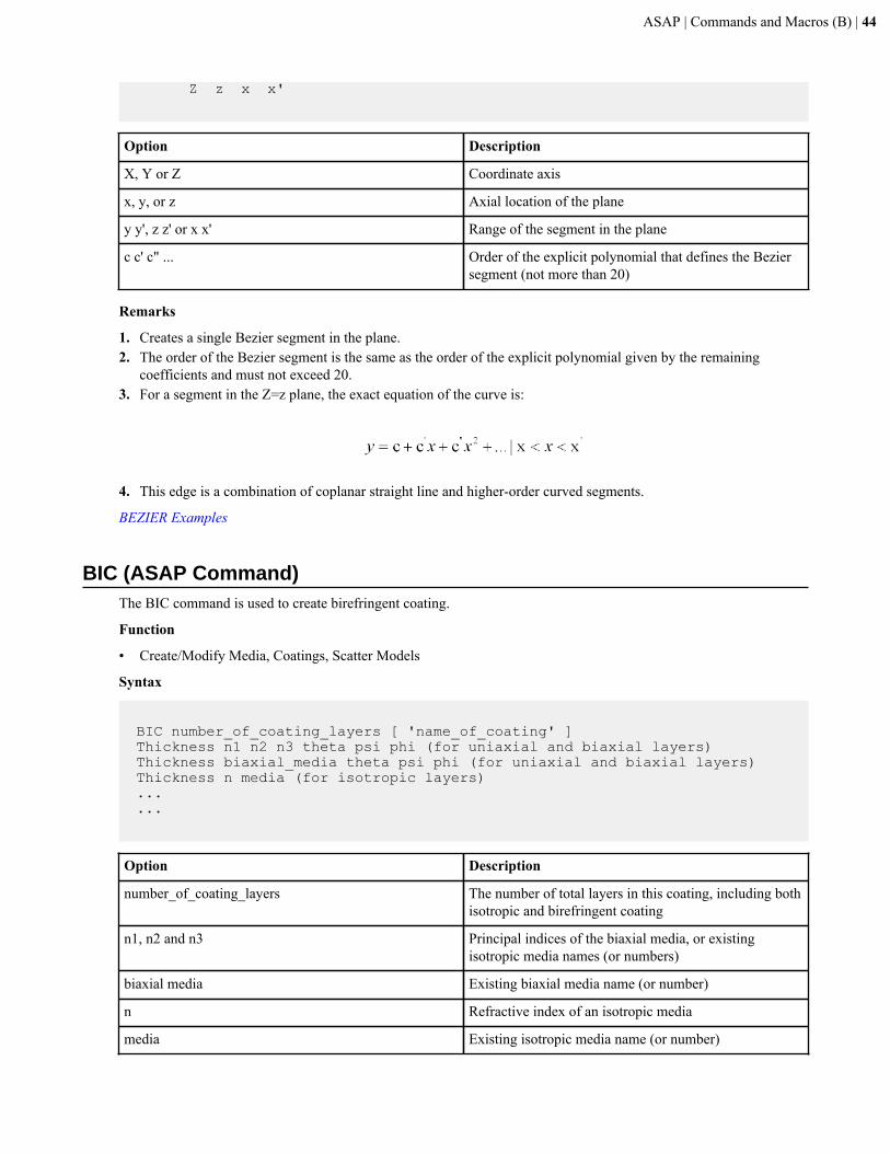
ASAP | Commands and Macros (B) | 44
Z z x x'
Option Description
X, Y or Z Coordinate axis
x, y, or z Axial location of the plane
y y', z z' or x x' Range of the segment in the plane
c c' c" ... Order of the explicit polynomial that defines the Beziersegment (not more than 20)
Remarks
1. Creates a single Bezier segment in the plane.2. The order of the Bezier segment is the same as the order of the explicit polynomial given by the remaining
coefficients and must not exceed 20.3. For a segment in the Z=z plane, the exact equation of the curve is:
4. This edge is a combination of coplanar straight line and higher-order curved segments.
BEZIER Examples
BIC (ASAP Command)The BIC command is used to create birefringent coating.
Function
• Create/Modify Media, Coatings, Scatter Models
Syntax
BIC number_of_coating_layers [ 'name_of_coating' ] Thickness n1 n2 n3 theta psi phi (for uniaxial and biaxial layers) Thickness biaxial_media theta psi phi (for uniaxial and biaxial layers) Thickness n media (for isotropic layers) ... ...
Option Description
number_of_coating_layers The number of total layers in this coating, including bothisotropic and birefringent coating
n1, n2 and n3 Principal indices of the biaxial media, or existingisotropic media names (or numbers)
biaxial media Existing biaxial media name (or number)
n Refractive index of an isotropic media
media Existing isotropic media name (or number)
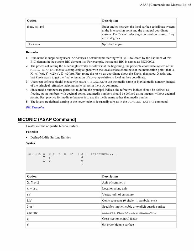
ASAP | Commands and Macros (B) | 45
Option Description
theta, psi, phi Euler angles between the local surface coordinate systemat the intersection point and the principal coordinatesystem. The Z-X-Z Euler angle convention is used. Theyare in degrees.
Thickness Specified in µm
Remarks
1. If no name is supplied by users, ASAP uses a default name starting with BIC, followed by the list index of thisBIC element in the system BIC element list. For example, the second BIC is named as BIC00002.
2. The process of setting the Euler angles works as follows: at the beginning, the principle coordinate system of theMEDIA BIAXIAL media is completely aligned with the local surface coordinate at the intersection point; that is,X->n1(xp), Y->n2(yp), Z->n3(zp). First rotate the xp-yp-zp coordinate about the Z axis, then about X axis, andlast Z axis again to get the final orientation of xp-yp-zp relative to local surface coordinate.
3. Users can define a biaxial media with MEDIA BIAXIAL to use the media name or biaxial media number, insteadof the principal refractive index numeric values in the BIC command.
4. Since media numbers are permitted to define the principal indices, the refractive indices should be defined asfloating-point numbers with decimal points, and media numbers should be defined using integers without decimalpoints. Best practice for media references is to use the media name rather than media number.
5. The layers are defined starting at the lower index side (usually air), as in the COATING LAYERS command.
BIC Examples
BICONIC (ASAP Command)Creates a cubic or quartic biconic surface.
Function
• Define/Modify Surfunc Entities
Syntax
BICONIC X x r r' k k' [ 3 ] [aperture... ] Y y 4 Z z q 6
Option Description
X, Y or Z Axis of symmetry
x, y or z Location along axis
r r' Vertex radii of curvature
k k' Conic constants (0 circle, -1 parabola, etc.)
3 or 4 Specifies implicit cubic or explicit quartic surface
aperture ELLIPSE, RECTANGLE, or HEXAGONAL
q Cross-section control factor
6 6th order biconic surface
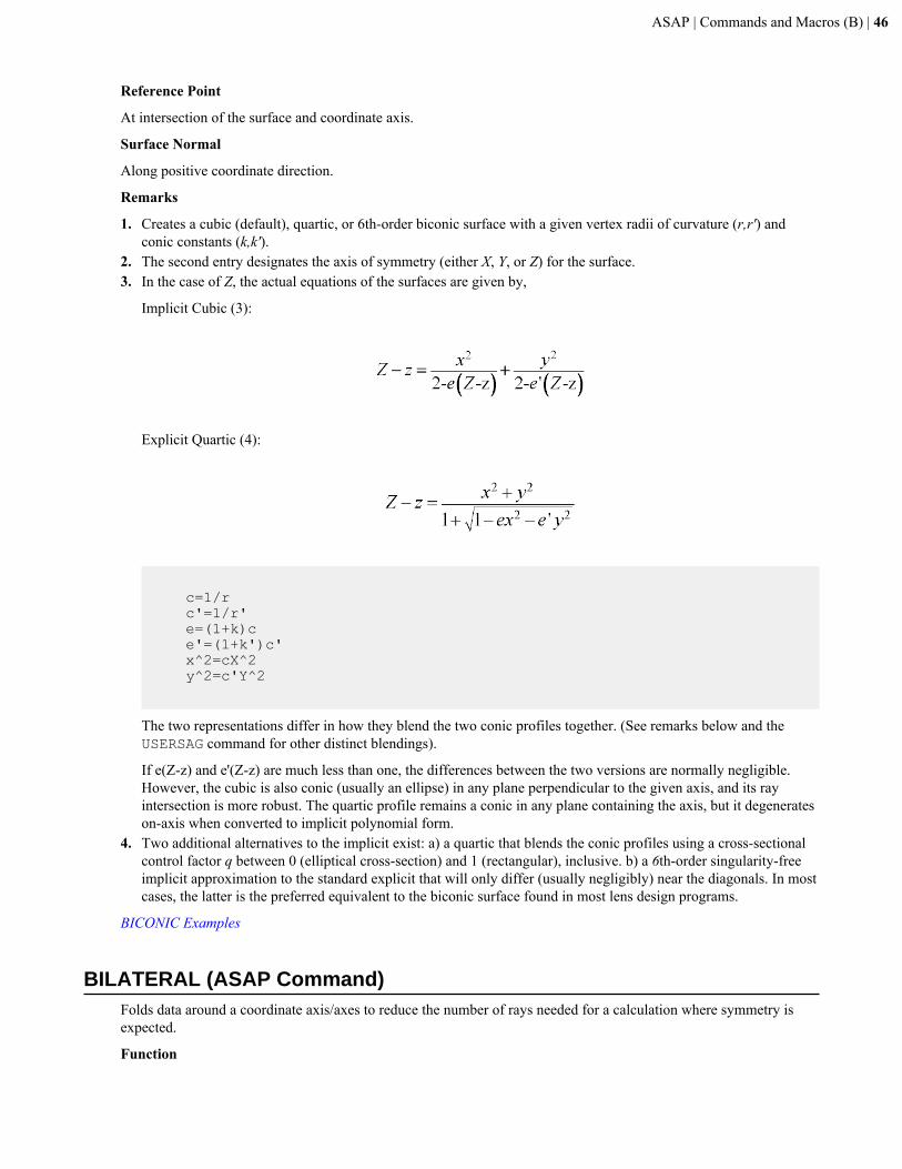
ASAP | Commands and Macros (B) | 46
Reference Point
At intersection of the surface and coordinate axis.
Surface Normal
Along positive coordinate direction.
Remarks
1. Creates a cubic (default), quartic, or 6th-order biconic surface with a given vertex radii of curvature (r,r') andconic constants (k,k').
2. The second entry designates the axis of symmetry (either X, Y, or Z) for the surface.3. In the case of Z, the actual equations of the surfaces are given by,
Implicit Cubic (3):
Explicit Quartic (4):
c=1/r c'=1/r' e=(1+k)c e'=(1+k')c' x^2=cX^2 y^2=c'Y^2
The two representations differ in how they blend the two conic profiles together. (See remarks below and theUSERSAG command for other distinct blendings).
If e(Z-z) and e'(Z-z) are much less than one, the differences between the two versions are normally negligible.However, the cubic is also conic (usually an ellipse) in any plane perpendicular to the given axis, and its rayintersection is more robust. The quartic profile remains a conic in any plane containing the axis, but it degenerateson-axis when converted to implicit polynomial form.
4. Two additional alternatives to the implicit exist: a) a quartic that blends the conic profiles using a cross-sectionalcontrol factor q between 0 (elliptical cross-section) and 1 (rectangular), inclusive. b) a 6th-order singularity-freeimplicit approximation to the standard explicit that will only differ (usually negligibly) near the diagonals. In mostcases, the latter is the preferred equivalent to the biconic surface found in most lens design programs.
BICONIC Examples
BILATERAL (ASAP Command)Folds data around a coordinate axis/axes to reduce the number of rays needed for a calculation where symmetry isexpected.
Function
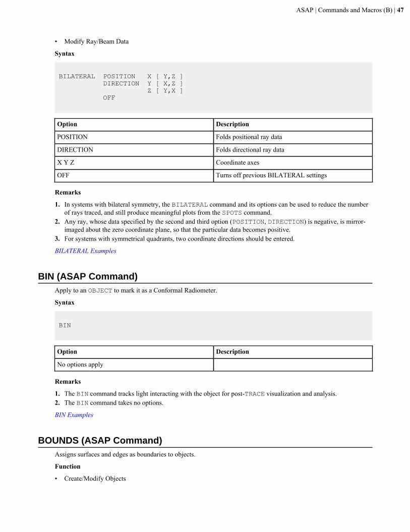
ASAP | Commands and Macros (B) | 47
• Modify Ray/Beam Data
Syntax
BILATERAL POSITION X [ Y,Z ] DIRECTION Y [ X,Z ] Z [ Y,X ] OFF
Option Description
POSITION Folds positional ray data
DIRECTION Folds directional ray data
X Y Z Coordinate axes
OFF Turns off previous BILATERAL settings
Remarks
1. In systems with bilateral symmetry, the BILATERAL command and its options can be used to reduce the numberof rays traced, and still produce meaningful plots from the SPOTS command.
2. Any ray, whose data specified by the second and third option (POSITION, DIRECTION) is negative, is mirror-imaged about the zero coordinate plane, so that the particular data becomes positive.
3. For systems with symmetrical quadrants, two coordinate directions should be entered.
BILATERAL Examples
BIN (ASAP Command)Apply to an OBJECT to mark it as a Conformal Radiometer.
Syntax
BIN
Option Description
No options apply
Remarks
1. The BIN command tracks light interacting with the object for post-TRACE visualization and analysis.2. The BIN command takes no options.
BIN Examples
BOUNDS (ASAP Command)Assigns surfaces and edges as boundaries to objects.
Function
• Create/Modify Objects
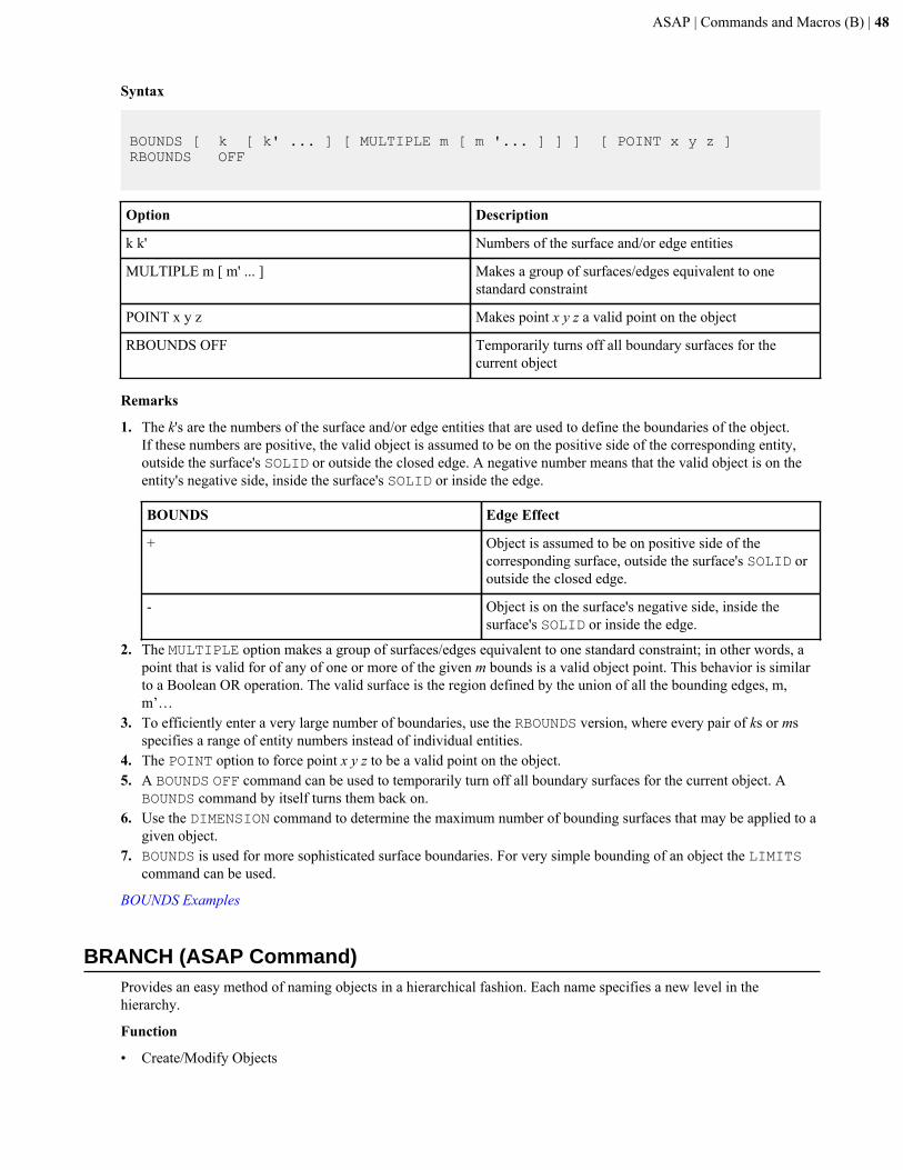
ASAP | Commands and Macros (B) | 48
Syntax
BOUNDS [ k [ k' ... ] [ MULTIPLE m [ m '... ] ] ] [ POINT x y z ]RBOUNDS OFF
Option Description
k k' Numbers of the surface and/or edge entities
MULTIPLE m [ m' ... ] Makes a group of surfaces/edges equivalent to onestandard constraint
POINT x y z Makes point x y z a valid point on the object
RBOUNDS OFF Temporarily turns off all boundary surfaces for thecurrent object
Remarks
1. The k's are the numbers of the surface and/or edge entities that are used to define the boundaries of the object.If these numbers are positive, the valid object is assumed to be on the positive side of the corresponding entity,outside the surface's SOLID or outside the closed edge. A negative number means that the valid object is on theentity's negative side, inside the surface's SOLID or inside the edge.
BOUNDS Edge Effect
+ Object is assumed to be on positive side of thecorresponding surface, outside the surface's SOLID oroutside the closed edge.
- Object is on the surface's negative side, inside thesurface's SOLID or inside the edge.
2. The MULTIPLE option makes a group of surfaces/edges equivalent to one standard constraint; in other words, apoint that is valid for of any of one or more of the given m bounds is a valid object point. This behavior is similarto a Boolean OR operation. The valid surface is the region defined by the union of all the bounding edges, m,m’…
3. To efficiently enter a very large number of boundaries, use the RBOUNDS version, where every pair of ks or msspecifies a range of entity numbers instead of individual entities.
4. The POINT option to force point x y z to be a valid point on the object.5. A BOUNDS OFF command can be used to temporarily turn off all boundary surfaces for the current object. A
BOUNDS command by itself turns them back on.6. Use the DIMENSION command to determine the maximum number of bounding surfaces that may be applied to a
given object.7. BOUNDS is used for more sophisticated surface boundaries. For very simple bounding of an object the LIMITS
command can be used.
BOUNDS Examples
BRANCH (ASAP Command)Provides an easy method of naming objects in a hierarchical fashion. Each name specifies a new level in thehierarchy.
Function
• Create/Modify Objects
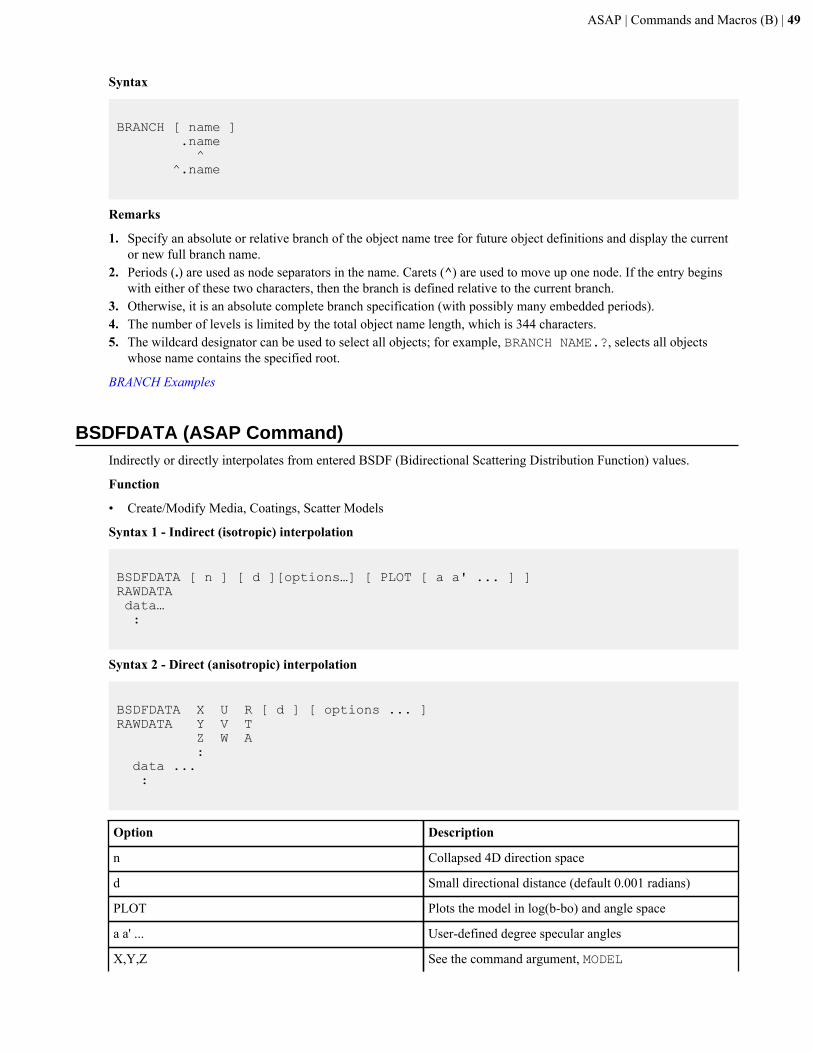
ASAP | Commands and Macros (B) | 49
Syntax
BRANCH [ name ] .name ^ ^.name
Remarks
1. Specify an absolute or relative branch of the object name tree for future object definitions and display the currentor new full branch name.
2. Periods (.) are used as node separators in the name. Carets (^) are used to move up one node. If the entry beginswith either of these two characters, then the branch is defined relative to the current branch.
3. Otherwise, it is an absolute complete branch specification (with possibly many embedded periods).4. The number of levels is limited by the total object name length, which is 344 characters.5. The wildcard designator can be used to select all objects; for example, BRANCH NAME.?, selects all objects
whose name contains the specified root.
BRANCH Examples
BSDFDATA (ASAP Command)Indirectly or directly interpolates from entered BSDF (Bidirectional Scattering Distribution Function) values.
Function
• Create/Modify Media, Coatings, Scatter Models
Syntax 1 - Indirect (isotropic) interpolation
BSDFDATA [ n ] [ d ][options…] [ PLOT [ a a' ... ] ] RAWDATA data… :
Syntax 2 - Direct (anisotropic) interpolation
BSDFDATA X U R [ d ] [ options ... ]RAWDATA Y V T Z W A : data ... :
Option Description
n Collapsed 4D direction space
d Small directional distance (default 0.001 radians)
PLOT Plots the model in log(b-bo) and angle space
a a' ... User-defined degree specular angles
X,Y,Z See the command argument, MODEL
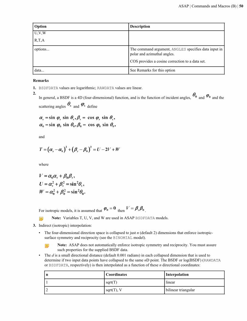
ASAP | Commands and Macros (B) | 50
Option DescriptionU,V,W
R,T,A
options... The command argument, ANGLES specifies data input inpolar and azimuthal angles.
COS provides a cosine correction to a data set.
data... See Remarks for this option
Remarks
1. BSDFDATA values are logarithmic; RAWDATA values are linear.2.
In general, a BSDF is a 4D (four-dimensional) function, and is the function of incident angles, and and the
scattering angles and define
and
where
For isotropic models, it is assumed that then .
Note: Variables T, U, V, and W are used in ASAP BSDFDATA models.
3. Indirect (isotropic) interpolation:
• The four-dimensional direction space is collapsed to just n (default 2) dimensions that enforce isotropic-surface symmetry and reciprocity (see the BINOMIAL model).
Note: ASAP does not automatically enforce isotropic symmetry and reciprocity. You must assuresuch properties for the supplied BSDF data.
• The d is a small directional distance (default 0.001 radians) in each collapsed dimension that is used todetermine if two input data points have collapsed to the same nD point. The BSDF or log(BSDF) (RAWDATAor BSDFDATA, respectively) is then interpolated as a function of these n directional coordinates:
n Coordinates Interpolation
1 sqrt(T) linear
2 sqrt(T), V bilinear triangular
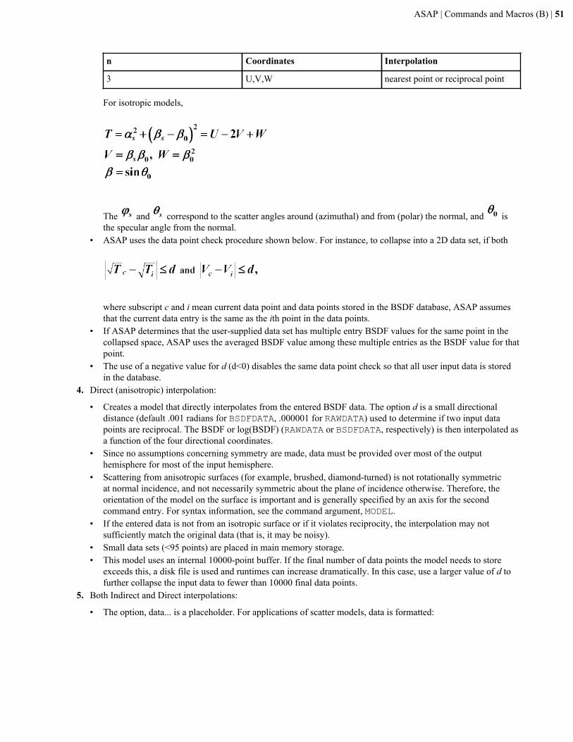
ASAP | Commands and Macros (B) | 51
n Coordinates Interpolation
3 U,V,W nearest point or reciprocal point
For isotropic models,
The and correspond to the scatter angles around (azimuthal) and from (polar) the normal, and isthe specular angle from the normal.
• ASAP uses the data point check procedure shown below. For instance, to collapse into a 2D data set, if both
where subscript c and i mean current data point and data points stored in the BSDF database, ASAP assumesthat the current data entry is the same as the ith point in the data points.
• If ASAP determines that the user-supplied data set has multiple entry BSDF values for the same point in thecollapsed space, ASAP uses the averaged BSDF value among these multiple entries as the BSDF value for thatpoint.
• The use of a negative value for d (d<0) disables the same data point check so that all user input data is storedin the database.
4. Direct (anisotropic) interpolation:
• Creates a model that directly interpolates from the entered BSDF data. The option d is a small directionaldistance (default .001 radians for BSDFDATA, .000001 for RAWDATA) used to determine if two input datapoints are reciprocal. The BSDF or log(BSDF) (RAWDATA or BSDFDATA, respectively) is then interpolated asa function of the four directional coordinates.
• Since no assumptions concerning symmetry are made, data must be provided over most of the outputhemisphere for most of the input hemisphere.
• Scattering from anisotropic surfaces (for example, brushed, diamond-turned) is not rotationally symmetricat normal incidence, and not necessarily symmetric about the plane of incidence otherwise. Therefore, theorientation of the model on the surface is important and is generally specified by an axis for the secondcommand entry. For syntax information, see the command argument, MODEL.
• If the entered data is not from an isotropic surface or if it violates reciprocity, the interpolation may notsufficiently match the original data (that is, it may be noisy).
• Small data sets (<95 points) are placed in main memory storage.• This model uses an internal 10000-point buffer. If the final number of data points the model needs to store
exceeds this, a disk file is used and runtimes can increase dramatically. In this case, use a larger value of d tofurther collapse the input data to fewer than 10000 final data points.
5. Both Indirect and Direct interpolations:
• The option, data... is a placeholder. For applications of scatter models, data is formatted:
ASAP | Commands and Macros (B) | 52
For applications of coating models, data is formatted:
•
For isotropic BSDF scatter models, must be 0.• Several BSDF models allow fitting to or interpolation from actual data. See the command argument, ANGLES
for common options and format.• The PLOT option plots the model (common base 10 logarithm of the BSDF) for up to seven specular angles
in ascending order (default 0, 15, 30, 45, 60, 75, 89.9 degrees). The current PIXELS setting controls theresolution of these plots in direction cosine space.
• Creates a distribution file name_angle.dis for each of these angles.• The command argument, MINMAX may be used to set the minimum and maximum values of the BSDF for this
specific model.• Works with a single normal-incidence scan.• Processed points are written TO and read FROM SYSTEM file.
BSDFDATA Examples
ASAP | Commands and Macros (C) | 53
Commands and Macros (C)
Topics in this section of the Contents tab include ASAP commands and macros that begin with the letter “C”.
CADEXPORT (ASAP Command)Writes out CAD-compatible system geometry file.
Function
• Save or Recover System Data
Syntax
CADEXPORT [ IGS [ name ] ] [ p a ] CADEXPORT DXF [ name [ block ] ] CADEXPORT VCR [ name ] CADEXPORT TRACE [ name [ vcr ] ]
Option Description
IGS Writes current geometry to an IGES file (the default)
DXF Writes current geometry to an AutoCAD DXF file usingAutoCAD 12 file format
VCR Reads geometry and rays from the current VCR file andwrites it to a DXF file
TRACE Reads only the rays from a named VCR file and writes itto an IGES file
name Names the output file to be written
block Holds the DXF file standards in the named file
vcr Names the VCR file from which ray data will be read bythe TRACE option
p The three-dimensional positional tolerance for IGESoutput, in system units
a The angular tolerance for IGES output, in degrees
Remarks
1. Writes a 3D CAD surface representation of the currently considered objects, or the 3D graphics in a VCR file, orjust the rays from the latest TRACE PLOT.
2. CADEXPORT supports the fixed IGES IGS (the default) and AutoCAD 12 DXF file standards (including theoption to put everything into a named block). The file created is name followed by one of these extensions: IGSfor IGES or DXF for AutoCAD 12.
3. CADEXPORT does not export a deformed surface that is produced in ASAP after a DEFORM command. The basesurface that is before DEFORM does export. Use the DEFORM command for phase / wavelength-level deformationsto base surfaces only in ASAP.
ASAP | Commands and Macros (C) | 54
4. The DXF and VCR options create DXF files; however, the DXF option converts from "system" geometry ratherthan the vector (VCR) file. BRO recommends you use the VCR option for DXF files to insure all trimming isconverted.
5. Trimming information (LIMITS, LOCAL, BOUNDS) is translated as of ASAP 2006 V1R1. BOUNDing entitiesmust have limiting apertures.
6. Limitations on surface export are:
• Advanced surface effects (REDEFINE SURF/NORM, DEFORM) are not translated.• IGS usually requires that the system UNITS must have been set.• All base surfaces in DXF are, by necessity, approximated by facets.• LENS, connected CURVE/EDGE, and SAMPLED base surfaces are exported exactly to IGES. Since no CAD
standard supports general algebraic surfaces, all other SURFACES are approximated by cubic spline patches orrevolved cubic spline curves when possible.
7. The TRACE option extracts ray trajectories from a VCR file vcr (ASAPTEMP.VCR by default), and writes therays to an IGES file name (ASAPTEMP.IGS by default).
CADEXPORT Examples
CARTOVAL (ASAP Command)Creates a Cartesian oval surface.
Function
• Define/Modify Surfunc Entities
Syntax
CARTOVAL X x d n d' n' [ aperture... ] Y y Z z
Option Description
X, Y, or Z Specifies axis of symmetry
x, y, or z Location along axis of symmetry
d Distance from surface to first focus point
n Refractive index of first medium
d' Distance from surface to second focus point
n' Refractive index of second medium
aperture ELLIPSE, RECTANGLE, or HEXAGONAL
Reference Point
At intersection of surface vertex and coordinate axis
Surface Normal
Along positive coordinate direction
Remarks
1. Creates a Cartesian Oval surface at the given location on the given axis.2. The second entry designates the axis of symmetry (either X, Y, or Z) for the surface.
ASAP | Commands and Macros (C) | 55
3. The surface perfectly images an axial point a distance d in the first medium of index n into an axial point adistance d' in the second medium of index n'
4. This surface can extend to infinity unless a LOCAL command follows, or a trailing aperture option of thefollowing form is specified:
ELLIPSE a [ a' [ o [ s [ s' ] ] ] ]RECTANGLEHEXAGONAL a [ o [ s [ s' ] ] ]
5. a a' are the heights in the other two transverse directions.6. For the HEXAGONAL form, a is the center-to-vertex distance (maximum height).7. o is an optional central hole ratio.8. s s' are the transverse coordinates of the center of the aperture.
CARTOVAL Examples
$CASE (ASAP Macro)Specifies case sensitivity.
Syntax
$CASE [ UPPER ] LOWER BOTH
Remarks
1. Macro instructs the parser to recognize only UPPER- or LOWER-case letters or BOTH.2. The case of the prompt displayed below the ASAP Command Input window reflects the setting of the $CASE
macro.3. If no argument is given on the command, the state before the last $CASE command is restored.4. Letters opposite in case to that set by the $CASE command can also be used as embedded comments, since
the program treats them as blanks. Trailing comments can be entered after an exclamation point "!", since thischaracter signals the program to stop decoding input from the command.
5. Opposite case letters: treated as blanks.6. Last entry, stop parsing: exclamation point.7. When using lower case for comments, do not include underscores "_" as these are treated as upper case and
generate an "Unrecognized command or macro" error.
$CASE Examples
CHARACTER (ASAP Command)Creates an edge of a specified string.
Function
• Define/Modify Curvedge Entities
Syntax
CHARACTER X x y [ z ] string
ASAP | Commands and Macros (C) | 56
Y y z x 'string' Z z x y
Option Description
X, Y or Z Character plane
x, y or z Character plane location
y, z or x Character width
z, x or y Character height (defaulted to the width)
string or 'string' Edge character string
Reference Point
First point of character
Remarks
1. Creates an edge patterned after the character string.2. This edge is a combination of coplanar straight line segments.
CHARACTER Examples
CHROMATICITY (ASAP Command)Calculates CIE tristimulus (XYZ) values and chromaticity (x,y) coordinates.
Function
• Analyze Ray/Beam Data
Syntax 1
CHROMATICITY INTENSITY|IRRADIANCE [SOM] [resolution] [NORM TF|MX|MY|MZ|CX| CY|CZ|AX|AY|AZ|nflux|xn, yn, X|Y|Z]
Syntax 2
CHROMATICITY RADIANT|RADIANCE [SOM] [resolution] [ANGLE X|Y|Z f f' n a a' n'] [NORM TF|MX|MY|MZ|CX|CY|CZ|AX|AY|AZ|nflux|xn, yn, X|Y|Z]
Option Description
CHROMATICITY INTENSITY/IRRADIANCE Calculates the chromaticity with radiance in the spatialcoordinate system, using the most recent WINDOW andPIXELS settings.
CHROMATICITY RADIANT/RADIANCE Calculates the chromaticity within the sphericalcoordinate system.
SOM Standard observer model for this colorimetry analysisconfiguration can be 1931 for 1931 2-degree observermodel or 1964 for 10-degree observer model.
resolution Wavelength resolution (in units of nm) for thisconfiguration. Must be an integer greater than 1. The

ASAP | Commands and Macros (C) | 57
Option Descriptionbuilt-in color matching functions for both the 1931 and1964 SOM standard are from 360nm to 830nm in 1nmresolution.
ANGLE X|Y|Z Polar angle
f f' Starting and ending polar (zenith/latitudinal) angles
n Number of polar subdivisions, must be 1 forCHROMATICITY RADIANCE option
a a' Starting and ending azimuthal (longitudinal) angles
n' Number of azimuthal subdivisions; must be 1 forCHROMATICITY RADIANCE option
NORM Normalization method for the tristimulus values.Currently, there are 14 ways to normalize XYZ values. IfNORM is not present, the default normalization method isthat the calculated tristimulus values are not normalized.If present, it must be in one of the following forms:
TF Normalization by the total flux of the rays used in thetristimulus calculation
MX, MY, MZ Normalization by the maximum values of the tristimulusvalues of X, Y, Z values
CX, CY, CZ Normalization by the X, Y, Z tristimulus values of thecenter pixel
AX, AY, AZ Normalization by the average values of tristimulusvalues of X, Y, Z nflux: normalization by the user-specified flux value, xn, yn: the spatial coordinate (x, y)in the sampling window of the pixel whose value is usedfor normalization
X|Y|Z X, Y, Z tristimulus value of the normalization pixel
Remarks
1. CHROMATICITY INTENSITY calculates the tristimulus values and chromaticity coordinates in a directioncosine coordinate system. The Y tristimulus value is computed in a direction cosine coordinate system, and it canbe converted to an angular coordinate system by using the ANGLES display modifier. The other components arecomputed in a direction cosine coordinate system; therefore, do not use the ANGLES display modifier, since itapplies a cosine modification to the distribution.
2. CHROMATICITY IRRADIANCE calculates the tristimulus values and chromaticity coordinates in a spatialcoordinate system.
3. CHROMATICITY RADIANT calculates the tristimulus values and chromaticity coordinates in a polar sphericalcoordinate system.
4. CHROMATICITY RADIANCE calculates the tristimulus values and chromaticity coordinates in a radianceformat; the spatial component is set with the current WINDOW and PIXEL settings, and the angular componentuses a polar spherical coordinate system that is set with the ANGLE option. See the RADIANT command for adescription of the ANGLE option.
When using CHROMATICITY RADIANT, the ANGLE parameters set the angular sampling window for both polarand azimuth angles. When using CHROMATICITY RADIANCE, the ANGLE parameter sets the sampling solidangle. Typically, the angular resolution for both polar and azimuth angle is set to a number greater than one (>1)for CHROMATICITY RADIANT and exactly one (=1) for CHROMATICITY RADIANCE.
ASAP | Commands and Macros (C) | 58
5. If the existing settings of SOM and/or the wavelength resolution of the current colorimetry analysis configurationare different from the new settings, all colorimetry analyses performed in this configuration are automaticallyupdated with the new SOM and/or wavelength resolution. These analyses include Lab, RGB, and LUV.
6. The CIE tristimulus (XYZ) and chromaticity coordinate (xy) values are calculated and saved in the distributionfile named as CIEXYZxy_ followed by the configuration name as entered on the most recent CIE command. Theorder of the tristimulus values and chromaticity coordinates in a data record of the output distribution file is X, Y,Z, x, y.
7. The CIE 1960, 1976 uniform color space chromaticity coordinate (uv), (u'v'), and correlated color temperature(CCT) are also calculated for each pixel and stored in the resulting distribution file in the order of u, v,u’, v’, and CCT after xy chromaticity. Therefore, a total of 10 CIE quantities exist for each pixel: X Y Ztristimulus, x y chromaticity 1931 CIE Standard, u v chromaticity in CIE 1960 uniform color space, u’ v’chromaticity in CIE 1976 uniform color space and correlated color temperature (CCT). Use DISPLAY"CIEXYZxy_CIE_configuration_name" first (1st) through tenth (10th) to access desired information.
8. Robertson's method[1] is used to determine the correlated color temperature (CCT). If the calculated CCT is outof the upper bound of the table (page 228), it is labeled as 1. If the calculated CCT is out of the lower bound ofthe table (page 228), it is labeled as -1. If the method is invalid, the CCT for that pixel, is labeled as 0. [1. ColorScience, Wyszechi and Stiles, second Edtion, pages 227-228 (2000).]
9. Multiple tristimulus value calculations (performed by multiple CHROMATICITY commands) can be carried outon a colorimetry analysis configuration.
10. See the topic, "SOM Option Matrix for CIE-CHROMATICITY Commands".
CHROMATICITY Examples
SOM Option Matrix for CIE-CHROMATICITY CommandsThis topic describes the SOM options matrix. The CIE command is intended to provide a single place to define userconfigurations of color calculations. The CHROMATICITY command is one type of color analysis that is controlledby the configuration, and others follow.
SOM Options Matrix
CIE Setting CHROMATICITY Setting Result
None None 1964
None 1964 1964
None 1931 1931
1964 None 1964
1964 1964 1964
1964 1931 1931
1931 None 1931
1931 1964 1964
1931 1931 1931
Summary
• The 1964 SOM is the default result if no SOM option is specified on either the CIE or CHROMATICITYcommand.
• If a SOM is specified with the CIE command, but is not specified with the CHROMATICITY command, the CIEoption is used.
• If a SOM is specified with the CHROMATICITY command, the specification on the CHROMATICITY commandoverrides that of the CIE command.

ASAP | Commands and Macros (C) | 59
Note: BRO recommends as a best practice to specify the SOM option on the CIE command. The overridingbehavior of the SOM option with theCHROMATICITY command should be used as an exception to your usualworkflow.
CIE-CHROMATICITY Resolution Options
The logic that coordinates the Resolution inputs to the CIE and CHROMATICITY commands is similar to the logicused for the SOM option:
• A 5-nm resolution is the default result if no Resolution option is specified on either the CIE or CHROMATICITYcommand.
• If the Resolution option is specified with the CIE command only (that is, none is specified with theCHROMATICITY command), the Resolution option of the CIE command is used.
• If Resolution is specified with the CHROMATICITY command, the specification on the CHROMATICITYcommand overrides that of the CIE command.
CIE (ASAP Command)Creates a new colorimetry analysis configuration or recalls an existing colorimetry analysis configuration.
Function
• Analyze Ray/Beam Data
Syntax 1
CIE NEW [SOM] [resolution] [‘name’]
Syntax 2
CIE ID|name [SOM] [resolution]
Option Description
SOM The standard observer model for this colorimetryanalysis configuration can be 1931 for the 1931 2-degreeobserver model, or 1964 for the 10-degree observermodel. The default is the 1964 10-degree observermodel.
resolution The wavelength resolution (in unit of nm) for thisconfiguration. Must be an integer greater than 1. If notspecified, the default resolution is 5nm. The built-incolor matching functions for both 1931 and 1964 SOMare from 360nm-830nm in 1nm resolution.
name Name of this colorimetry analysis configuration. It mustbe no longer than 40 characters and is case insensitive.If no name is specified, ASAP uses the default name inthe form of CACXXXXX, where XXXXX is the indexof the configuration. The configuration can be retrievedby its name or its index in the defined configuration list.
ID The index of the colorimetry configuration that the userwants to retrieve.
ASAP | Commands and Macros (C) | 60
Remarks
1. Before any colorimetry analysis, a colorimetry analysis configuration must be created. The default maximumnumber of colorimetry analysis configurations in ASAP is 25; users can change this with SET MNCC to anynumber.
2. The normal work flow of ASAP colorimetry is similar to the traditional four-step ASAP work flow, except theanalysis step replaced by the colorimetry analysis step.
3. As in classic ASAP radiometric analysis, specific ray set can be selected in ASAP colorimetry analysis with theSELECT command, and interested objects can be selected with the CONSIDER command. Also, the parametersof analysis window can be set with WINDOW and PIXEL commands. These parameters must be set before CIEanalysis can be performed.
4. The analysis results are saved to distribution files denoted with its configuration name. For example,the CIEtristimulus and chromaticity coordinate values generated by a CHROMATICITY command are saved in adistribution file named as CIEXYZxy_ followed by the configuration name entered on the most recent CIEcommand.
5. For any colorimetry analysis configuration, the wavelengths of sources must be in units of nm.6. Syntax 2 is used to recall or modify an existing colorimetry analysis configuration.7. If a configuration is recalled with a different SOM or different wavelength resolution other than its previous
settings, all colorimetry analysis performed in this configuration is automatically updated with the new SOM and/or wavelength resolution.
8. See the topic, "SOM Option Matrix for CIE-CHROMATICITY Commands".
CIE Examples
SOM Option Matrix for CIE-CHROMATICITY CommandsThis topic describes the SOM options matrix. The CIE command is intended to provide a single place to define userconfigurations of color calculations. The CHROMATICITY command is one type of color analysis that is controlledby the configuration, and others follow.
SOM Options Matrix
CIE Setting CHROMATICITY Setting Result
None None 1964
None 1964 1964
None 1931 1931
1964 None 1964
1964 1964 1964
1964 1931 1931
1931 None 1931
1931 1964 1964
1931 1931 1931
Summary
• The 1964 SOM is the default result if no SOM option is specified on either the CIE or CHROMATICITYcommand.
• If a SOM is specified with the CIE command, but is not specified with the CHROMATICITY command, the CIEoption is used.
• If a SOM is specified with the CHROMATICITY command, the specification on the CHROMATICITY commandoverrides that of the CIE command.
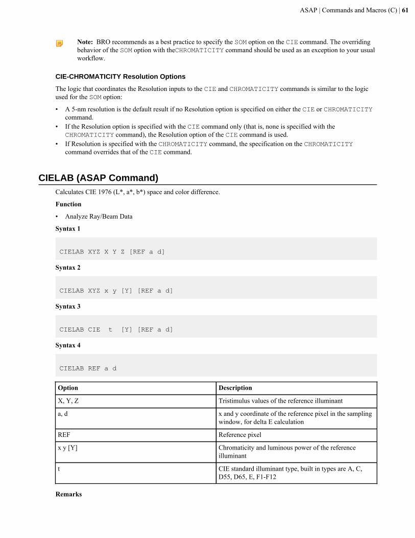
ASAP | Commands and Macros (C) | 61
Note: BRO recommends as a best practice to specify the SOM option on the CIE command. The overridingbehavior of the SOM option with theCHROMATICITY command should be used as an exception to your usualworkflow.
CIE-CHROMATICITY Resolution Options
The logic that coordinates the Resolution inputs to the CIE and CHROMATICITY commands is similar to the logicused for the SOM option:
• A 5-nm resolution is the default result if no Resolution option is specified on either the CIE or CHROMATICITYcommand.
• If the Resolution option is specified with the CIE command only (that is, none is specified with theCHROMATICITY command), the Resolution option of the CIE command is used.
• If Resolution is specified with the CHROMATICITY command, the specification on the CHROMATICITYcommand overrides that of the CIE command.
CIELAB (ASAP Command)Calculates CIE 1976 (L*, a*, b*) space and color difference.
Function
• Analyze Ray/Beam Data
Syntax 1
CIELAB XYZ X Y Z [REF a d]
Syntax 2
CIELAB XYZ x y [Y] [REF a d]
Syntax 3
CIELAB CIE t [Y] [REF a d]
Syntax 4
CIELAB REF a d
Option Description
X, Y, Z Tristimulus values of the reference illuminant
a, d x and y coordinate of the reference pixel in the samplingwindow, for delta E calculation
REF Reference pixel
x y [Y] Chromaticity and luminous power of the referenceilluminant
t CIE standard illuminant type, built in types are A, C,D55, D65, E, F1-F12
Remarks
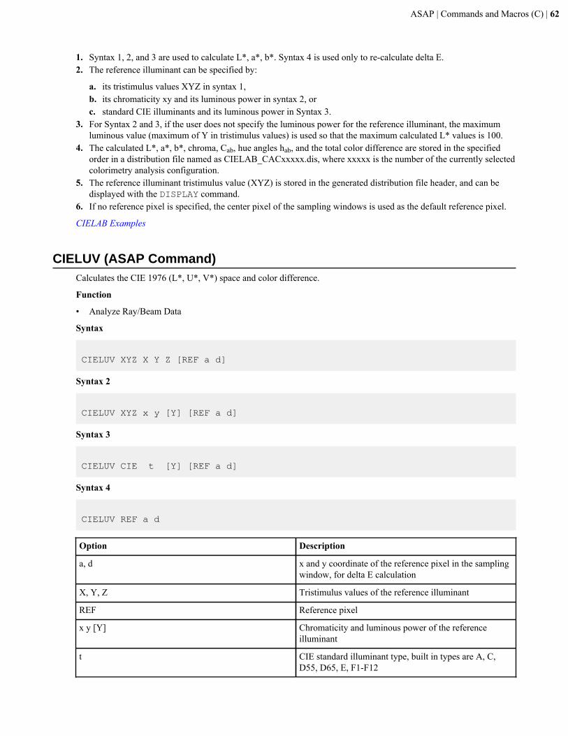
ASAP | Commands and Macros (C) | 62
1. Syntax 1, 2, and 3 are used to calculate L*, a*, b*. Syntax 4 is used only to re-calculate delta E.2. The reference illuminant can be specified by:
a. its tristimulus values XYZ in syntax 1,b. its chromaticity xy and its luminous power in syntax 2, orc. standard CIE illuminants and its luminous power in Syntax 3.
3. For Syntax 2 and 3, if the user does not specify the luminous power for the reference illuminant, the maximumluminous value (maximum of Y in tristimulus values) is used so that the maximum calculated L* values is 100.
4. The calculated L*, a*, b*, chroma, Cab, hue angles hab, and the total color difference are stored in the specifiedorder in a distribution file named as CIELAB_CACxxxxx.dis, where xxxxx is the number of the currently selectedcolorimetry analysis configuration.
5. The reference illuminant tristimulus value (XYZ) is stored in the generated distribution file header, and can bedisplayed with the DISPLAY command.
6. If no reference pixel is specified, the center pixel of the sampling windows is used as the default reference pixel.
CIELAB Examples
CIELUV (ASAP Command)Calculates the CIE 1976 (L*, U*, V*) space and color difference.
Function
• Analyze Ray/Beam Data
Syntax
CIELUV XYZ X Y Z [REF a d]
Syntax 2
CIELUV XYZ x y [Y] [REF a d]
Syntax 3
CIELUV CIE t [Y] [REF a d]
Syntax 4
CIELUV REF a d
Option Description
a, d x and y coordinate of the reference pixel in the samplingwindow, for delta E calculation
X, Y, Z Tristimulus values of the reference illuminant
REF Reference pixel
x y [Y] Chromaticity and luminous power of the referenceilluminant
t CIE standard illuminant type, built in types are A, C,D55, D65, E, F1-F12
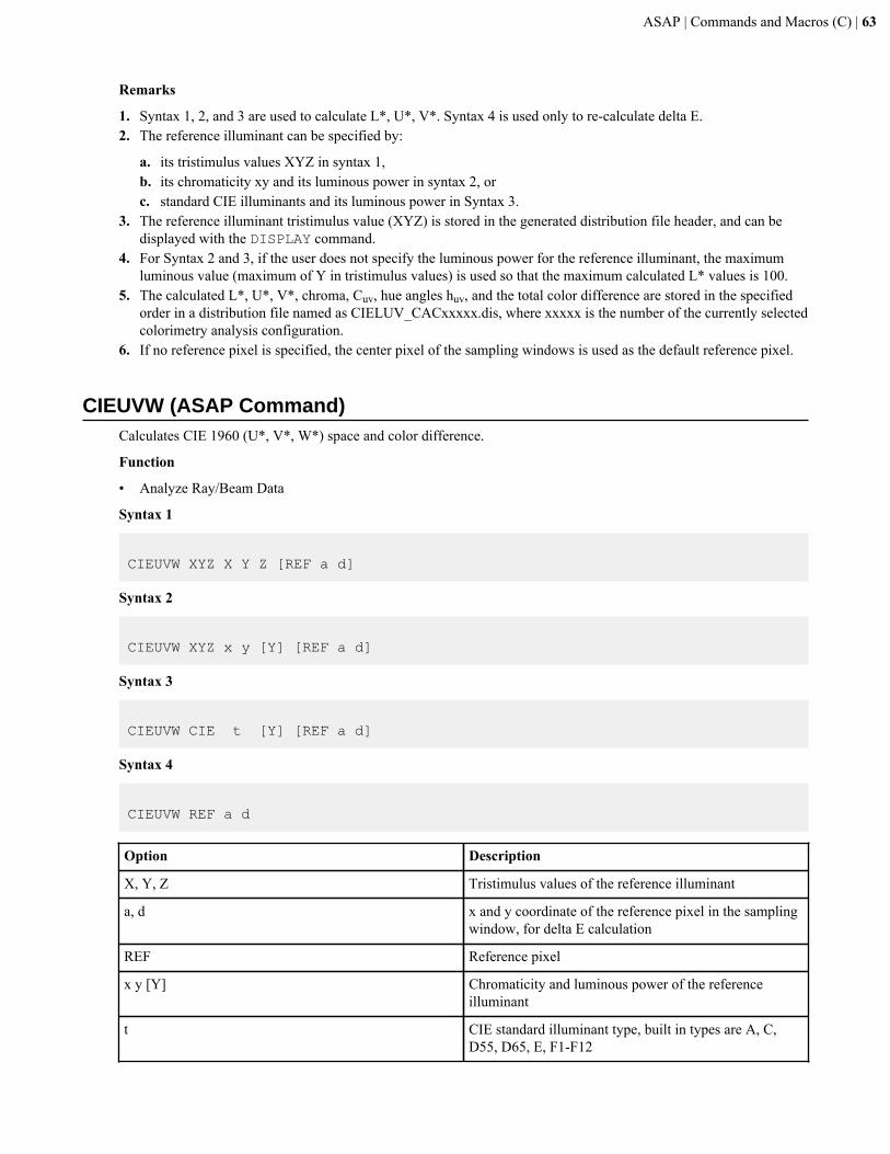
ASAP | Commands and Macros (C) | 63
Remarks
1. Syntax 1, 2, and 3 are used to calculate L*, U*, V*. Syntax 4 is used only to re-calculate delta E.2. The reference illuminant can be specified by:
a. its tristimulus values XYZ in syntax 1,b. its chromaticity xy and its luminous power in syntax 2, orc. standard CIE illuminants and its luminous power in Syntax 3.
3. The reference illuminant tristimulus value (XYZ) is stored in the generated distribution file header, and can bedisplayed with the DISPLAY command.
4. For Syntax 2 and 3, if the user does not specify the luminous power for the reference illuminant, the maximumluminous value (maximum of Y in tristimulus values) is used so that the maximum calculated L* values is 100.
5. The calculated L*, U*, V*, chroma, Cuv, hue angles huv, and the total color difference are stored in the specifiedorder in a distribution file named as CIELUV_CACxxxxx.dis, where xxxxx is the number of the currently selectedcolorimetry analysis configuration.
6. If no reference pixel is specified, the center pixel of the sampling windows is used as the default reference pixel.
CIEUVW (ASAP Command)Calculates CIE 1960 (U*, V*, W*) space and color difference.
Function
• Analyze Ray/Beam Data
Syntax 1
CIEUVW XYZ X Y Z [REF a d]
Syntax 2
CIEUVW XYZ x y [Y] [REF a d]
Syntax 3
CIEUVW CIE t [Y] [REF a d]
Syntax 4
CIEUVW REF a d
Option Description
X, Y, Z Tristimulus values of the reference illuminant
a, d x and y coordinate of the reference pixel in the samplingwindow, for delta E calculation
REF Reference pixel
x y [Y] Chromaticity and luminous power of the referenceilluminant
t CIE standard illuminant type, built in types are A, C,D55, D65, E, F1-F12
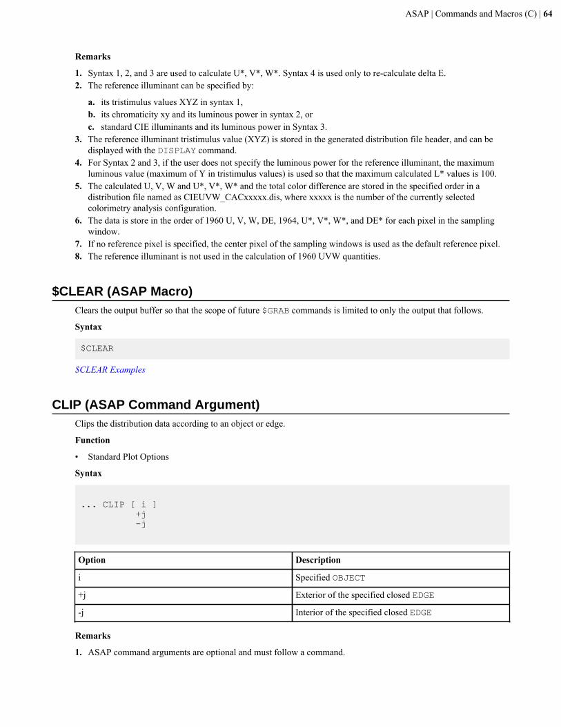
ASAP | Commands and Macros (C) | 64
Remarks
1. Syntax 1, 2, and 3 are used to calculate U*, V*, W*. Syntax 4 is used only to re-calculate delta E.2. The reference illuminant can be specified by:
a. its tristimulus values XYZ in syntax 1,b. its chromaticity xy and its luminous power in syntax 2, orc. standard CIE illuminants and its luminous power in Syntax 3.
3. The reference illuminant tristimulus value (XYZ) is stored in the generated distribution file header, and can bedisplayed with the DISPLAY command.
4. For Syntax 2 and 3, if the user does not specify the luminous power for the reference illuminant, the maximumluminous value (maximum of Y in tristimulus values) is used so that the maximum calculated L* values is 100.
5. The calculated U, V, W and U*, V*, W* and the total color difference are stored in the specified order in adistribution file named as CIEUVW_CACxxxxx.dis, where xxxxx is the number of the currently selectedcolorimetry analysis configuration.
6. The data is store in the order of 1960 U, V, W, DE, 1964, U*, V*, W*, and DE* for each pixel in the samplingwindow.
7. If no reference pixel is specified, the center pixel of the sampling windows is used as the default reference pixel.8. The reference illuminant is not used in the calculation of 1960 UVW quantities.
$CLEAR (ASAP Macro)Clears the output buffer so that the scope of future $GRAB commands is limited to only the output that follows.
Syntax
$CLEAR
$CLEAR Examples
CLIP (ASAP Command Argument)Clips the distribution data according to an object or edge.
Function
• Standard Plot Options
Syntax
... CLIP [ i ] +j -j
Option Description
i Specified OBJECT
+j Exterior of the specified closed EDGE
-j Interior of the specified closed EDGE
Remarks
1. ASAP command arguments are optional and must follow a command.
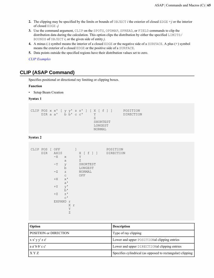
ASAP | Commands and Macros (C) | 65
2. The clipping may be specified by the limits or bounds of OBJECT i the exterior of closed EDGE +j or the interiorof closed EDGE -j
3. Use the command argument, CLIP on the SPOTS, OPDMAP, SPREAD, or FIELD commands to clip thedistribution data during the calculation. This option clips the distribution by either the specified LIMITS/BOUNDS of OBJECT i, or the given side of entity j.
4. A minus (-) symbol means the interior of a closed EDGE or the negative side of a SURFACE. A plus (+) symbolmeans the exterior of a closed EDGE or the positive side of a SURFACE.
5. Data points outside the specified regions have their distribution values set to zero.
CLIP Examples
CLIP (ASAP Command)Specifies positional or directional ray limiting or clipping boxes.
Function
• Setup Beam Creation
Syntax 1
CLIP POS x x' [ y y' z z' ] [ X [ f ] ] POSITION DIR a a' b b' c c' Y DIRECTION Z SHORTEST LONGEST NORMAL
Syntax 2
CLIP POS [ OFF ] POSITION DIR AXIS X [ f ] ] DIRECTION -X x Y a Z -Y y SHORTEST b LONGEST -Z z NORMAL c OFF +X x' a' +Y y' b' +Z z' c' EXPAND r X r Y Z
Option Description
POSITION or DIRECTION Type of ray clipping
x x' y y' z z' Lower and upper POSITIONal clipping entries
a a' b b' c c' Lower and upper DIRECTIONal clipping entries
X Y Z Specifies cylindrical (as opposed to rectangular) clipping
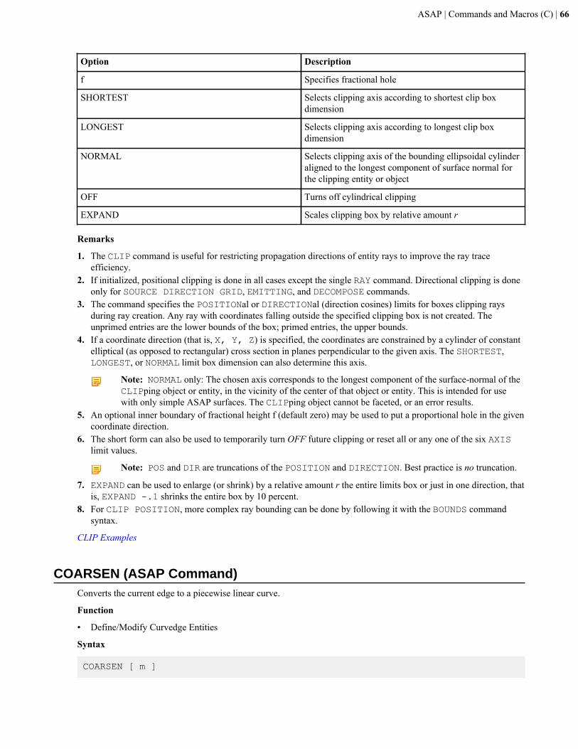
ASAP | Commands and Macros (C) | 66
Option Description
f Specifies fractional hole
SHORTEST Selects clipping axis according to shortest clip boxdimension
LONGEST Selects clipping axis according to longest clip boxdimension
NORMAL Selects clipping axis of the bounding ellipsoidal cylinderaligned to the longest component of surface normal forthe clipping entity or object
OFF Turns off cylindrical clipping
EXPAND Scales clipping box by relative amount r
Remarks
1. The CLIP command is useful for restricting propagation directions of entity rays to improve the ray traceefficiency.
2. If initialized, positional clipping is done in all cases except the single RAY command. Directional clipping is doneonly for SOURCE DIRECTION GRID, EMITTING, and DECOMPOSE commands.
3. The command specifies the POSITIONal or DIRECTIONal (direction cosines) limits for boxes clipping raysduring ray creation. Any ray with coordinates falling outside the specified clipping box is not created. Theunprimed entries are the lower bounds of the box; primed entries, the upper bounds.
4. If a coordinate direction (that is, X, Y, Z) is specified, the coordinates are constrained by a cylinder of constantelliptical (as opposed to rectangular) cross section in planes perpendicular to the given axis. The SHORTEST,LONGEST, or NORMAL limit box dimension can also determine this axis.
Note: NORMAL only: The chosen axis corresponds to the longest component of the surface-normal of theCLIPping object or entity, in the vicinity of the center of that object or entity. This is intended for usewith only simple ASAP surfaces. The CLIPping object cannot be faceted, or an error results.
5. An optional inner boundary of fractional height f (default zero) may be used to put a proportional hole in the givencoordinate direction.
6. The short form can also be used to temporarily turn OFF future clipping or reset all or any one of the six AXISlimit values.
Note: POS and DIR are truncations of the POSITION and DIRECTION. Best practice is no truncation.
7. EXPAND can be used to enlarge (or shrink) by a relative amount r the entire limits box or just in one direction, thatis, EXPAND -.1 shrinks the entire box by 10 percent.
8. For CLIP POSITION, more complex ray bounding can be done by following it with the BOUNDS commandsyntax.
CLIP Examples
COARSEN (ASAP Command)Converts the current edge to a piecewise linear curve.
Function
• Define/Modify Curvedge Entities
Syntax
COARSEN [ m ]
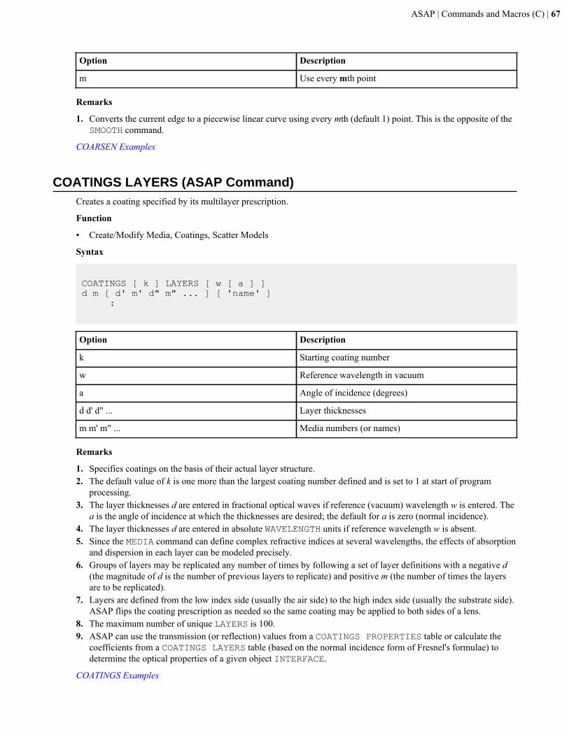
ASAP | Commands and Macros (C) | 67
Option Description
m Use every mth point
Remarks
1. Converts the current edge to a piecewise linear curve using every mth (default 1) point. This is the opposite of theSMOOTH command.
COARSEN Examples
COATINGS LAYERS (ASAP Command)Creates a coating specified by its multilayer prescription.
Function
• Create/Modify Media, Coatings, Scatter Models
Syntax
COATINGS [ k ] LAYERS [ w [ a ] ]d m [ d' m' d" m" ... ] [ 'name' ] :
Option Description
k Starting coating number
w Reference wavelength in vacuum
a Angle of incidence (degrees)
d d' d" ... Layer thicknesses
m m' m" ... Media numbers (or names)
Remarks
1. Specifies coatings on the basis of their actual layer structure.2. The default value of k is one more than the largest coating number defined and is set to 1 at start of program
processing.3. The layer thicknesses d are entered in fractional optical waves if reference (vacuum) wavelength w is entered. The
a is the angle of incidence at which the thicknesses are desired; the default for a is zero (normal incidence).4. The layer thicknesses d are entered in absolute WAVELENGTH units if reference wavelength w is absent.5. Since the MEDIA command can define complex refractive indices at several wavelengths, the effects of absorption
and dispersion in each layer can be modeled precisely.6. Groups of layers may be replicated any number of times by following a set of layer definitions with a negative d
(the magnitude of d is the number of previous layers to replicate) and positive m (the number of times the layersare to be replicated).
7. Layers are defined from the low index side (usually the air side) to the high index side (usually the substrate side).ASAP flips the coating prescription as needed so the same coating may be applied to both sides of a lens.
8. The maximum number of unique LAYERS is 100.9. ASAP can use the transmission (or reflection) values from a COATINGS PROPERTIES table or calculate the
coefficients from a COATINGS LAYERS table (based on the normal incidence form of Fresnel's formulae) todetermine the optical properties of a given object INTERFACE.
COATINGS Examples
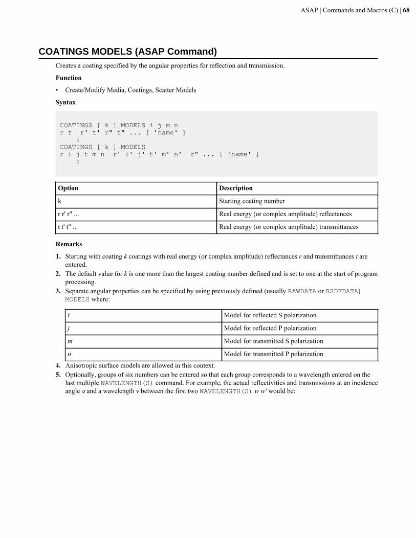
ASAP | Commands and Macros (C) | 68
COATINGS MODELS (ASAP Command)Creates a coating specified by the angular properties for reflection and transmission.
Function
• Create/Modify Media, Coatings, Scatter Models
Syntax
COATINGS [ k ] MODELS i j m n r t r' t' r" t" ... [ 'name' ] :COATINGS [ k ] MODELSr i j t m n r' i' j' t' m' n' r" ... [ 'name' ] :
Option Description
k Starting coating number
r r' r" ... Real energy (or complex amplitude) reflectances
t t' t" ... Real energy (or complex amplitude) transmittances
Remarks
1. Starting with coating k coatings with real energy (or complex amplitude) reflectances r and transmittances t areentered.
2. The default value for k is one more than the largest coating number defined and is set to one at the start of programprocessing.
3. Separate angular properties can be specified by using previously defined (usually RAWDATA or BSDFDATA)MODELS where:
i Model for reflected S polarization
j Model for reflected P polarization
m Model for transmitted S polarization
n Model for transmitted P polarization
4. Anisotropic surface models are allowed in this context.5. Optionally, groups of six numbers can be entered so that each group corresponds to a wavelength entered on the
last multiple WAVELENGTH(S) command. For example, the actual reflectivities and transmissions at an incidenceangle a and a wavelength v between the first two WAVELENGTH(S) w w' would be:
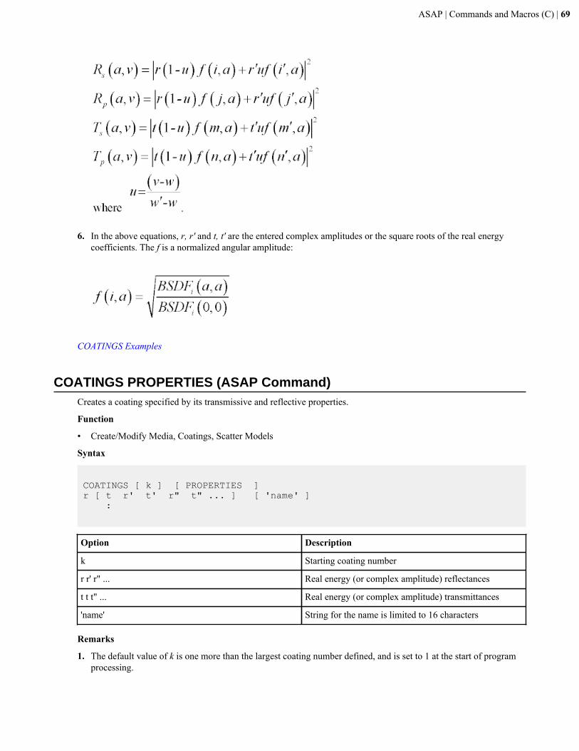
ASAP | Commands and Macros (C) | 69
6. In the above equations, r, r' and t, t' are the entered complex amplitudes or the square roots of the real energy
coefficients. The f is a normalized angular amplitude:
COATINGS Examples
COATINGS PROPERTIES (ASAP Command)Creates a coating specified by its transmissive and reflective properties.
Function
• Create/Modify Media, Coatings, Scatter Models
Syntax
COATINGS [ k ] [ PROPERTIES ]r [ t r' t' r" t" ... ] [ 'name' ] :
Option Description
k Starting coating number
r r' r" ... Real energy (or complex amplitude) reflectances
t t t" ... Real energy (or complex amplitude) transmittances
'name' String for the name is limited to 16 characters
Remarks
1. The default value of k is one more than the largest coating number defined, and is set to 1 at the start of programprocessing.
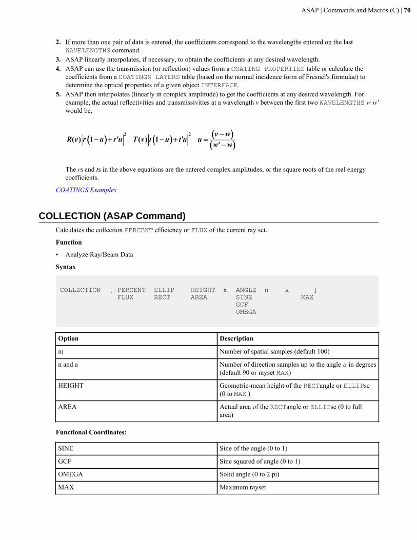
ASAP | Commands and Macros (C) | 70
2. If more than one pair of data is entered, the coefficients correspond to the wavelengths entered on the lastWAVELENGTHS command.
3. ASAP linearly interpolates, if necessary, to obtain the coefficients at any desired wavelength.4. ASAP can use the transmission (or reflection) values from a COATING PROPERTIES table or calculate the
coefficients from a COATINGS LAYERS table (based on the normal incidence form of Fresnel's formulae) todetermine the optical properties of a given object INTERFACE.
5. ASAP then interpolates (linearly in complex amplitude) to get the coefficients at any desired wavelength. Forexample, the actual reflectivities and transmissivities at a wavelength v between the first two WAVELENGTHS w w'would be,
The rs and ts in the above equations are the entered complex amplitudes, or the square roots of the real energycoefficients.
COATINGS Examples
COLLECTION (ASAP Command)Calculates the collection PERCENT efficiency or FLUX of the current ray set.
Function
• Analyze Ray/Beam Data
Syntax
COLLECTION [ PERCENT ELLIP HEIGHT m ANGLE n a ] FLUX RECT AREA SINE MAX GCF OMEGA
Option Description
m Number of spatial samples (default 100)
n and a Number of direction samples up to the angle a in degrees(default 90 or rayset MAX)
HEIGHT Geometric-mean height of the RECTangle or ELLIPse(0 to MAX )
AREA Actual area of the RECTangle or ELLIPse (0 to fullarea)
Functional Coordinates:
SINE Sine of the angle (0 to 1)
GCF Sine squared of angle (0 to 1)
OMEGA Solid angle (0 to 2 pi)
MAX Maximum rayset
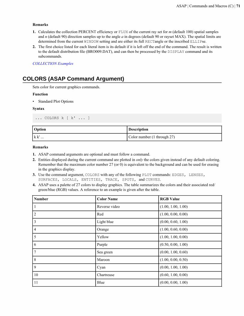
ASAP | Commands and Macros (C) | 71
Remarks
1. Calculates the collection PERCENT efficiency or FLUX of the current ray set for m (default 100) spatial samplesand n (default 90) direction samples up to the angle a in degrees (default 90 or rayset MAX). The spatial limits aredetermined from the current WINDOW setting and are either its full RECTangle or the inscribed ELLIPse.
2. The first choice listed for each literal item is its default if it is left off the end of the command. The result is writtento the default distribution file (BRO009.DAT), and can then be processed by the DISPLAY command and itssubcommands.
COLLECTION Examples
COLORS (ASAP Command Argument)Sets color for current graphics commands.
Function
• Standard Plot Options
Syntax
... COLORS k [ k' ... ]
Option Description
k k' ... Color number (1 through 27)
Remarks
1. ASAP command arguments are optional and must follow a command.2. Entities displayed during the current command are plotted in only the colors given instead of any default coloring.
Remember that the maximum color number 27 (or 0) is equivalent to the background and can be used for erasingin the graphics display.
3. Use the command argument, COLORS with any of the following PLOT commands: EDGES, LENSES,SURFACES, LOCALS, ENTITIES, TRACE, SPOTS, and CURVES.
4. ASAP uses a palette of 27 colors to display graphics. The table summarizes the colors and their associated red/green/blue (RGB) values. A reference to an example is given after the table.
Number Color Name RGB Value
1 Reverse video (1.00, 1.00, 1.00)
2 Red (1.00, 0.00, 0.00)
3 Light blue (0.00, 0.60, 1.00)
4 Orange (1.00, 0.60, 0.00)
5 Yellow (1.00, 1.00, 0.00)
6 Purple (0.50, 0.00, 1.00)
7 Sea green (0.00, 1.00, 0.60)
8 Maroon (1.00, 0.00, 0.50)
9 Cyan (0.00, 1.00, 1.00)
10 Chartreuse (0.60, 1.00, 0.00)
11 Blue (0.00, 0.00, 1.00)
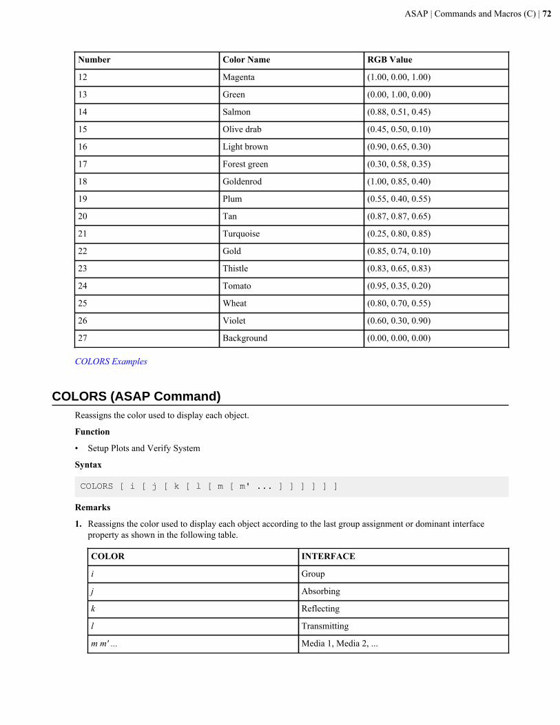
ASAP | Commands and Macros (C) | 72
Number Color Name RGB Value
12 Magenta (1.00, 0.00, 1.00)
13 Green (0.00, 1.00, 0.00)
14 Salmon (0.88, 0.51, 0.45)
15 Olive drab (0.45, 0.50, 0.10)
16 Light brown (0.90, 0.65, 0.30)
17 Forest green (0.30, 0.58, 0.35)
18 Goldenrod (1.00, 0.85, 0.40)
19 Plum (0.55, 0.40, 0.55)
20 Tan (0.87, 0.87, 0.65)
21 Turquoise (0.25, 0.80, 0.85)
22 Gold (0.85, 0.74, 0.10)
23 Thistle (0.83, 0.65, 0.83)
24 Tomato (0.95, 0.35, 0.20)
25 Wheat (0.80, 0.70, 0.55)
26 Violet (0.60, 0.30, 0.90)
27 Background (0.00, 0.00, 0.00)
COLORS Examples
COLORS (ASAP Command)Reassigns the color used to display each object.
Function
• Setup Plots and Verify System
Syntax
COLORS [ i [ j [ k [ l [ m [ m' ... ] ] ] ] ] ]
Remarks
1. Reassigns the color used to display each object according to the last group assignment or dominant interfaceproperty as shown in the following table.
COLOR INTERFACE
i Group
j Absorbing
k Reflecting
l Transmitting
m m' ... Media 1, Media 2, ...
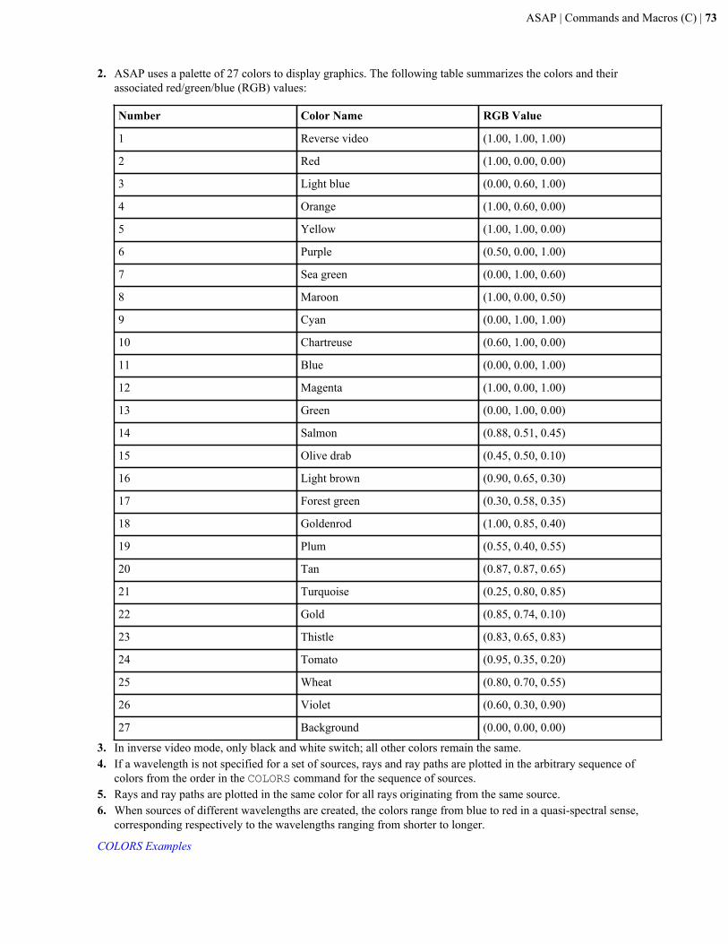
ASAP | Commands and Macros (C) | 73
2. ASAP uses a palette of 27 colors to display graphics. The following table summarizes the colors and theirassociated red/green/blue (RGB) values:
Number Color Name RGB Value
1 Reverse video (1.00, 1.00, 1.00)
2 Red (1.00, 0.00, 0.00)
3 Light blue (0.00, 0.60, 1.00)
4 Orange (1.00, 0.60, 0.00)
5 Yellow (1.00, 1.00, 0.00)
6 Purple (0.50, 0.00, 1.00)
7 Sea green (0.00, 1.00, 0.60)
8 Maroon (1.00, 0.00, 0.50)
9 Cyan (0.00, 1.00, 1.00)
10 Chartreuse (0.60, 1.00, 0.00)
11 Blue (0.00, 0.00, 1.00)
12 Magenta (1.00, 0.00, 1.00)
13 Green (0.00, 1.00, 0.00)
14 Salmon (0.88, 0.51, 0.45)
15 Olive drab (0.45, 0.50, 0.10)
16 Light brown (0.90, 0.65, 0.30)
17 Forest green (0.30, 0.58, 0.35)
18 Goldenrod (1.00, 0.85, 0.40)
19 Plum (0.55, 0.40, 0.55)
20 Tan (0.87, 0.87, 0.65)
21 Turquoise (0.25, 0.80, 0.85)
22 Gold (0.85, 0.74, 0.10)
23 Thistle (0.83, 0.65, 0.83)
24 Tomato (0.95, 0.35, 0.20)
25 Wheat (0.80, 0.70, 0.55)
26 Violet (0.60, 0.30, 0.90)
27 Background (0.00, 0.00, 0.00)
3. In inverse video mode, only black and white switch; all other colors remain the same.4. If a wavelength is not specified for a set of sources, rays and ray paths are plotted in the arbitrary sequence of
colors from the order in the COLORS command for the sequence of sources.5. Rays and ray paths are plotted in the same color for all rays originating from the same source.6. When sources of different wavelengths are created, the colors range from blue to red in a quasi-spectral sense,
corresponding respectively to the wavelengths ranging from shorter to longer.
COLORS Examples
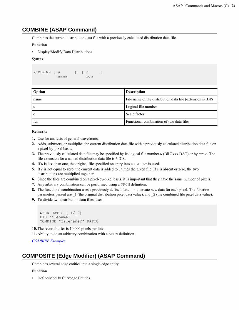
ASAP | Commands and Macros (C) | 74
COMBINE (ASAP Command)Combines the current distribution data file with a previously calculated distribution data file.
Function
• Display/Modify Data Distributions
Syntax
COMBINE [ u ] [ c ] name fcn
Option Description
name File name of the distribution data file (extension is .DIS)
u Logical file number
c Scale factor
fcn Functional combination of two data files
Remarks
1. Use for analysis of general wavefronts.2. Adds, subtracts, or multiplies the current distribution data file with a previously calculated distribution data file on
a pixel-by-pixel basis.3. The previously calculated data file may be specified by its logical file number u (BROxxx.DAT) or by name. The
file extension for a named distribution data file is *.DIS.4. If u is less than one, the original file specified on entry into DISPLAY is used.5. If c is not equal to zero, the current data is added to c times the given file. If c is absent or zero, the two
distributions are multiplied together.6. Since the files are combined on a pixel-by-pixel basis, it is important that they have the same number of pixels.7. Any arbitrary combination can be performed using a $FCN definition.8. The functional combination uses a previously defined function to create new data for each pixel. The function
parameters passed are _1 (the original distribution pixel data value), and _2 (the combined file pixel data value).9. To divide two distribution data files, use:
$FCN RATIO (_1/_2)DIS filename1COMBINE "filename2" RATIO
10. The record buffer is 10,000 pixels per line.11. Ability to do an arbitrary combination with a $FCN definition.
COMBINE Examples
COMPOSITE (Edge Modifier) (ASAP Command)Combines several edge entities into a single edge entity.
Function
• Define/Modify Curvedge Entities
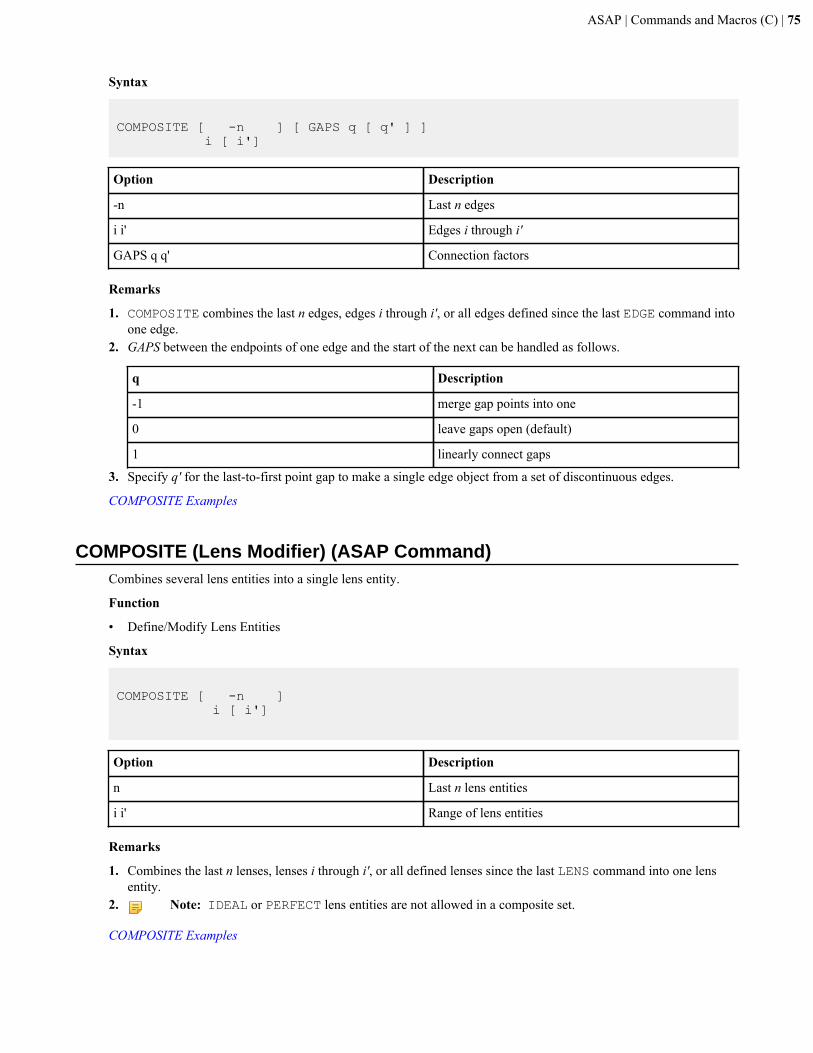
ASAP | Commands and Macros (C) | 75
Syntax
COMPOSITE [ -n ] [ GAPS q [ q' ] ] i [ i']
Option Description
-n Last n edges
i i' Edges i through i'
GAPS q q' Connection factors
Remarks
1. COMPOSITE combines the last n edges, edges i through i', or all edges defined since the last EDGE command intoone edge.
2. GAPS between the endpoints of one edge and the start of the next can be handled as follows.
q Description
-1 merge gap points into one
0 leave gaps open (default)
1 linearly connect gaps
3. Specify q' for the last-to-first point gap to make a single edge object from a set of discontinuous edges.
COMPOSITE Examples
COMPOSITE (Lens Modifier) (ASAP Command)Combines several lens entities into a single lens entity.
Function
• Define/Modify Lens Entities
Syntax
COMPOSITE [ -n ] i [ i']
Option Description
n Last n lens entities
i i' Range of lens entities
Remarks
1. Combines the last n lenses, lenses i through i', or all defined lenses since the last LENS command into one lensentity.
2. Note: IDEAL or PERFECT lens entities are not allowed in a composite set.
COMPOSITE Examples
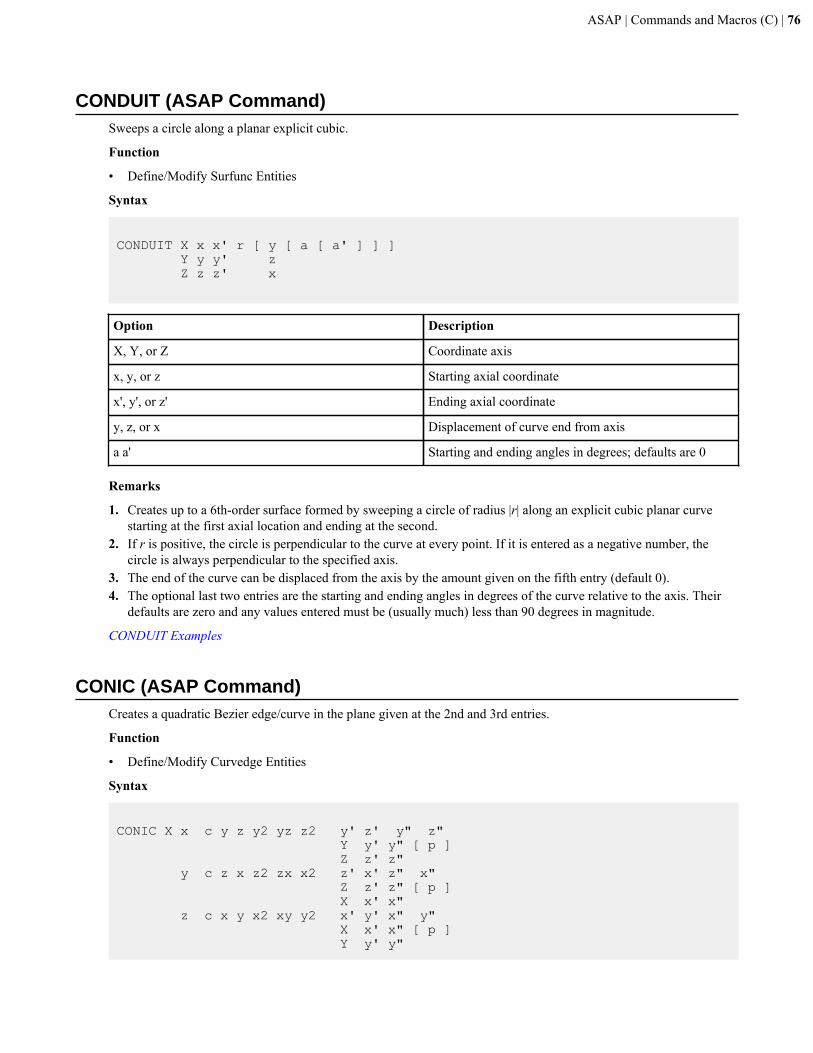
ASAP | Commands and Macros (C) | 76
CONDUIT (ASAP Command)Sweeps a circle along a planar explicit cubic.
Function
• Define/Modify Surfunc Entities
Syntax
CONDUIT X x x' r [ y [ a [ a' ] ] ] Y y y' z Z z z' x
Option Description
X, Y, or Z Coordinate axis
x, y, or z Starting axial coordinate
x', y', or z' Ending axial coordinate
y, z, or x Displacement of curve end from axis
a a' Starting and ending angles in degrees; defaults are 0
Remarks
1. Creates up to a 6th-order surface formed by sweeping a circle of radius |r| along an explicit cubic planar curvestarting at the first axial location and ending at the second.
2. If r is positive, the circle is perpendicular to the curve at every point. If it is entered as a negative number, thecircle is always perpendicular to the specified axis.
3. The end of the curve can be displaced from the axis by the amount given on the fifth entry (default 0).4. The optional last two entries are the starting and ending angles in degrees of the curve relative to the axis. Their
defaults are zero and any values entered must be (usually much) less than 90 degrees in magnitude.
CONDUIT Examples
CONIC (ASAP Command)Creates a quadratic Bezier edge/curve in the plane given at the 2nd and 3rd entries.
Function
• Define/Modify Curvedge Entities
Syntax
CONIC X x c y z y2 yz z2 y' z' y" z" Y y' y" [ p ] Z z' z" y c z x z2 zx x2 z' x' z" x" Z z' z" [ p ] X x' x" z c x y x2 xy y2 x' y' x" y" X x' x" [ p ] Y y' y"
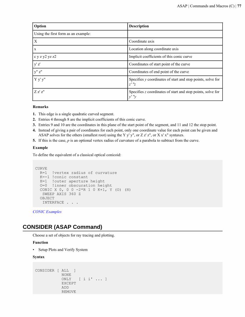
ASAP | Commands and Macros (C) | 77
Option Description
Using the first form as an example:
X Coordinate axis
x Location along coordinate axis
c y z y2 yz z2 Implicit coefficients of this conic curve
y' z' Coordinates of start point of the curve
y" z" Coordinates of end point of the curve
Y y' y" Specifies y coordinates of start and stop points, solve forz' "z
Z z' z" Specifies z coordinates of start and stop points, solve fory' "y
Remarks
1. This edge is a single quadratic curved segment.2. Entries 4 through 8 are the implicit coefficients of this conic curve.3. Entries 9 and 10 are the coordinates in this plane of the start point of the segment, and 11 and 12 the stop point.4. Instead of giving a pair of coordinates for each point, only one coordinate value for each point can be given and
ASAP solves for the others (smallest root) using the Y y' y", or Z z' z", or X x' x" syntaxes.5. If this is the case, p is an optional vertex radius of curvature of a parabola to subtract from the curve.
Example
To define the equivalent of a classical optical conicoid:
CURVE R=1 !vertex radius of curvature K=-1 !conic constant H=1 !outer aperture height O=0 !inner obscuration height CONIC X 0, 0 0 -2*R 1 0 K+1, Y (O) (H) SWEEP AXIS 360 Z OBJECT INTERFACE . . .
CONIC Examples
CONSIDER (ASAP Command)Choose a set of objects for ray tracing and plotting.
Function
• Setup Plots and Verify System
Syntax
CONSIDER [ ALL ] NONE ONLY [ i i' ... ] EXCEPT ADD REMOVE

ASAP | Commands and Macros (C) | 78
Option Description
ALL Consider all known objects
NONE Consider no objects
ONLY Consider only the objects specified (default is the currentGROUP)
i i' ... OBJECT numbers or names to be considered
EXCEPT Consider all objects except those specified (default is thecurrent GROUP)
ADD Adds the specified objects to the previous CONSIDERcommand
REMOVE Removes the specified objects from the previousCONSIDER command
Remarks
1. The CONSIDER command is used to isolate geometry, as well as all rays currently associated with that geometry.2. Provides control over the current set of objects that ASAP is to consider in all calculations and output. All objects
remain in the database at all times (that is, even when they are temporarily ignored with options other than ALL,they are not deleted).
3. By default all objects in the system database are CONSIDERed.4. A CONSIDER command by itself (with no entries) produces a list of the currently CONSIDERed objects.5. The EXCEPT option restricts the current object set to all objects except those specified (default is the current
GROUP). All objects except those specified may be drawn, ray traced, or analyzed.6. Particular object numbers (or names with "?" wildcards) can be either excluded with the EXCEPT option or be the
ONLY ones CONSIDERed. If no object list is given, the last GROUP is used.7. The current state (that is, a previous CONSIDER command) can be updated using ADD or REMOVE instead of
ONLY or EXCEPT, respectively.8. The ADD option adds the specified objects to the CONSIDER list. REMOVE subtracts the specified objects from the
CONSIDER list.9. Ray data are initially referenced by OBJECT 0. Before ray tracing, CONSIDER EXCEPT 0 effectively turns off
the ray data while maintaining all other geometry.10. When using OBJECT names, you can use only 40 characters in the name when you CONSIDER them.
CONSIDER Examples
CONTOUR (ASAP Command)Creates a contour plot of the current distribution data file.
Function
• Display/Modify Data Distributions
Syntax
CONTOUR n [ LOW ] [ TICS t [ t' ] ] [ VECTOR ] [ 'title' ] c' [ c" ... ] HIGH GRID
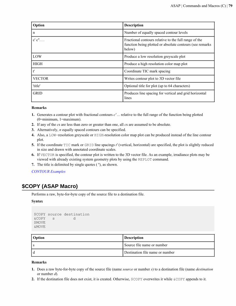
ASAP | Commands and Macros (C) | 79
Option Description
n Number of equally spaced contour levels
c' c". . . Fractional contours relative to the full range of thefunction being plotted or absolute contours (see remarksbelow)
LOW Produce a low resolution greyscale plot
HIGH Produce a high resolution color map plot
t' Coordinate TIC mark spacing
VECTOR Writes contour plot to 3D vector file
'title' Optional title for plot (up to 64 characters)
GRID Produces line spacing for vertical and grid horizontallines
Remarks
1. Generates a contour plot with fractional contours c' ... relative to the full range of the function being plotted(0=minimum, 1=maximum).
2. If any of the cs are less than zero or greater than one, all cs are assumed to be absolute.3. Alternatively, n equally spaced contours can be specified.4. Also, a LOW-resolution greyscale or HIGH-resolution color map plot can be produced instead of the line contour
plot.5. If the coordinate TIC mark or GRID line spacings t' (vertical, horizontal) are specified, the plot is slightly reduced
in size and drawn with annotated coordinate scales.6. If VECTOR is specified, the contour plot is written to the 3D vector file. As an example, irradiance plots may be
viewed with already existing system geometry plots by using the REPLOT command.7. The title is delimited by single quotes ( '), as shown.
CONTOUR Examples
$COPY (ASAP Macro)Performs a raw, byte-for-byte copy of the source file to a destination file.
Syntax
$COPY source destination© s d$MOVE&MOVE
Option Description
s Source file name or number
d Destination file name or number
Remarks
1. Does a raw byte-for-byte copy of the source file (name source or number s) to a destination file (name destinationor number d).
2. If the destination file does not exist, it is created. Otherwise, $COPY overwrites it while © appends to it.
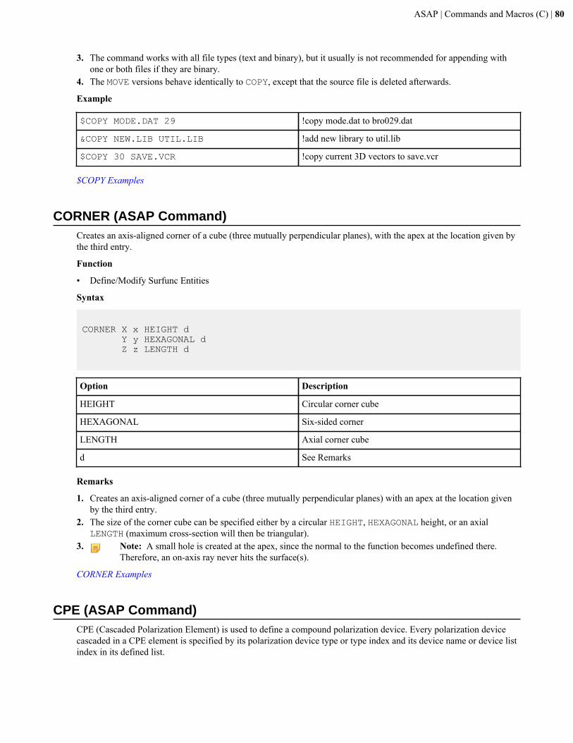
ASAP | Commands and Macros (C) | 80
3. The command works with all file types (text and binary), but it usually is not recommended for appending withone or both files if they are binary.
4. The MOVE versions behave identically to COPY, except that the source file is deleted afterwards.
Example
$COPY MODE.DAT 29 !copy mode.dat to bro029.dat
© NEW.LIB UTIL.LIB !add new library to util.lib
$COPY 30 SAVE.VCR !copy current 3D vectors to save.vcr
$COPY Examples
CORNER (ASAP Command)Creates an axis-aligned corner of a cube (three mutually perpendicular planes), with the apex at the location given bythe third entry.
Function
• Define/Modify Surfunc Entities
Syntax
CORNER X x HEIGHT d Y y HEXAGONAL d Z z LENGTH d
Option Description
HEIGHT Circular corner cube
HEXAGONAL Six-sided corner
LENGTH Axial corner cube
d See Remarks
Remarks
1. Creates an axis-aligned corner of a cube (three mutually perpendicular planes) with an apex at the location givenby the third entry.
2. The size of the corner cube can be specified either by a circular HEIGHT, HEXAGONAL height, or an axialLENGTH (maximum cross-section will then be triangular).
3. Note: A small hole is created at the apex, since the normal to the function becomes undefined there.Therefore, an on-axis ray never hits the surface(s).
CORNER Examples
CPE (ASAP Command)CPE (Cascaded Polarization Element) is used to define a compound polarization device. Every polarization devicecascaded in a CPE element is specified by its polarization device type or type index and its device name or device listindex in its defined list.
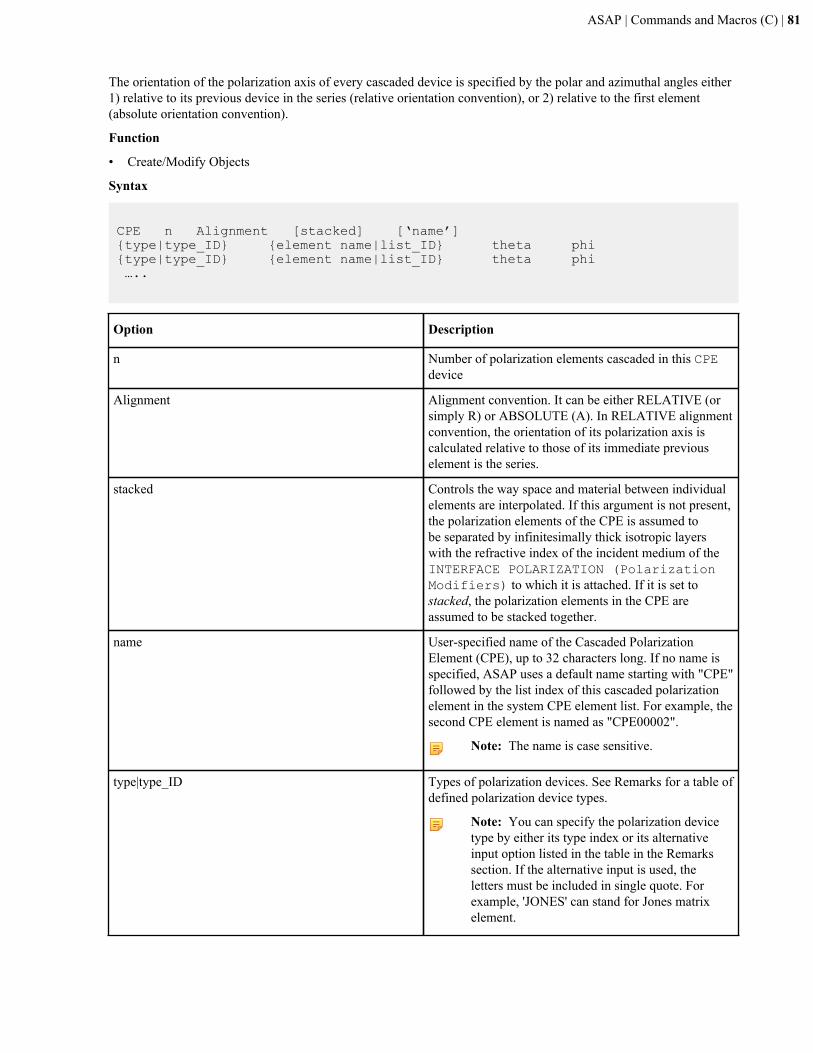
ASAP | Commands and Macros (C) | 81
The orientation of the polarization axis of every cascaded device is specified by the polar and azimuthal angles either1) relative to its previous device in the series (relative orientation convention), or 2) relative to the first element(absolute orientation convention).
Function
• Create/Modify Objects
Syntax
CPE n Alignment [stacked] [‘name’] {type|type_ID} {element name|list_ID} theta phi{type|type_ID} {element name|list_ID} theta phi …..
Option Description
n Number of polarization elements cascaded in this CPEdevice
Alignment Alignment convention. It can be either RELATIVE (orsimply R) or ABSOLUTE (A). In RELATIVE alignmentconvention, the orientation of its polarization axis iscalculated relative to those of its immediate previouselement is the series.
stacked Controls the way space and material between individualelements are interpolated. If this argument is not present,the polarization elements of the CPE is assumed tobe separated by infinitesimally thick isotropic layerswith the refractive index of the incident medium of theINTERFACE POLARIZATION (PolarizationModifiers) to which it is attached. If it is set tostacked, the polarization elements in the CPE areassumed to be stacked together.
name User-specified name of the Cascaded PolarizationElement (CPE), up to 32 characters long. If no name isspecified, ASAP uses a default name starting with "CPE"followed by the list index of this cascaded polarizationelement in the system CPE element list. For example, thesecond CPE element is named as "CPE00002".
Note: The name is case sensitive.
type|type_ID Types of polarization devices. See Remarks for a table ofdefined polarization device types.
Note: You can specify the polarization devicetype by either its type index or its alternativeinput option listed in the table in the Remarkssection. If the alternative input is used, theletters must be included in single quote. Forexample, 'JONES' can stand for Jones matrixelement.
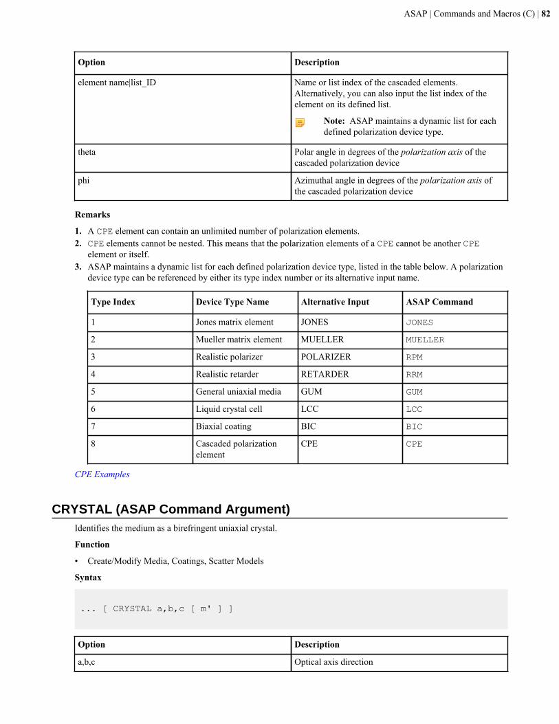
ASAP | Commands and Macros (C) | 82
Option Description
element name|list_ID Name or list index of the cascaded elements.Alternatively, you can also input the list index of theelement on its defined list.
Note: ASAP maintains a dynamic list for eachdefined polarization device type.
theta Polar angle in degrees of the polarization axis of thecascaded polarization device
phi Azimuthal angle in degrees of the polarization axis ofthe cascaded polarization device
Remarks
1. A CPE element can contain an unlimited number of polarization elements.2. CPE elements cannot be nested. This means that the polarization elements of a CPE cannot be another CPE
element or itself.3. ASAP maintains a dynamic list for each defined polarization device type, listed in the table below. A polarization
device type can be referenced by either its type index number or its alternative input name.
Type Index Device Type Name Alternative Input ASAP Command
1 Jones matrix element JONES JONES
2 Mueller matrix element MUELLER MUELLER
3 Realistic polarizer POLARIZER RPM
4 Realistic retarder RETARDER RRM
5 General uniaxial media GUM GUM
6 Liquid crystal cell LCC LCC
7 Biaxial coating BIC BIC
8 Cascaded polarizationelement
CPE CPE
CPE Examples
CRYSTAL (ASAP Command Argument)Identifies the medium as a birefringent uniaxial crystal.
Function
• Create/Modify Media, Coatings, Scatter Models
Syntax
... [ CRYSTAL a,b,c [ m' ] ]
Option Description
a,b,c Optical axis direction

ASAP | Commands and Macros (C) | 83
Option Description
m' Previous medium
Remarks
1. The command argument, CRYSTAL, identifies the medium as a birefringent uniaxial crystal with optical axisdirection a,b,c, and given extraordinary refractive indices.
2. Ordinary indices are specified on a previous medium m' (default is last). For example, a calcite crystal with itsoptical axis initially aligned along the Y direction is defined as follows:
MEDIA 1.66 !ordinary index for following extraordinary 1.49 CRYSTAL 0 1 0 =CALCITE
3. If SPLIT is one or higher, ASAP automatically generates an ordinary and an extraordinary ray/beam at eachcrystal interface.
4. If you linearly transform an object (for example, rotation) assigned a birefringent MEDIA, the lineartransformation is applied also to the optical axis direction of the medium. Any other object using this mediumis therefore affected. Thus, if a ROTATE or MATRIX command is applied to one object using the CRYSTALmedium, the medium itself is transformed and its instances on previous object interfaces are also affected. Thiseffect might be avoided by applying the transformation to the entity before it is used to form the object.
CRYSTAL Examples
CUTOFF (ASAP Command)Sets the conditions controlling ray termination.
Function
• Setup Trace
Syntax
CUTOFF [ t ] [ n ]
Option Description
t Absolute flux threshold (must be in decimal format)
n Maximum number of total object intersections for anyray (must be in integer format)
Remarks
1. Causes rays to be ignored.2. Sets the absolute flux threshold; below this value, ASAP ignores the rays to the decimal number t (default 1.E-18).3. The maximum number of total object intersections for any ray can be set to the integer n (default 1000).4. Tracing of CUTOFF rays cannot be continued.
CUTOFF Examples
CVF (ASAP Command)The CVF (Complex Vector Field) command provides a bidirectional translation facility between ASAP and FDTDSolutions™ by Lumerical.
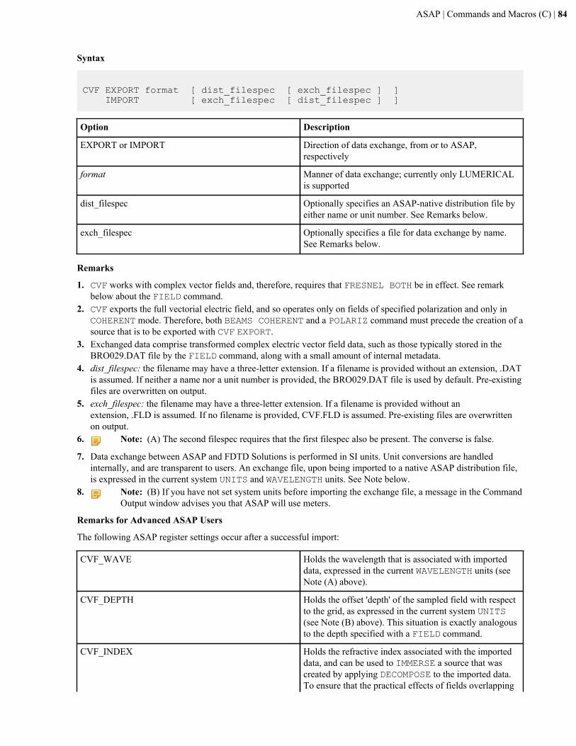
ASAP | Commands and Macros (C) | 84
Syntax
CVF EXPORT format [ dist_filespec [ exch_filespec ] ] IMPORT [ exch_filespec [ dist_filespec ] ]
Option Description
EXPORT or IMPORT Direction of data exchange, from or to ASAP,respectively
format Manner of data exchange; currently only LUMERICALis supported
dist_filespec Optionally specifies an ASAP-native distribution file byeither name or unit number. See Remarks below.
exch_filespec Optionally specifies a file for data exchange by name.See Remarks below.
Remarks
1. CVF works with complex vector fields and, therefore, requires that FRESNEL BOTH be in effect. See remarkbelow about the FIELD command.
2. CVF exports the full vectorial electric field, and so operates only on fields of specified polarization and only inCOHERENT mode. Therefore, both BEAMS COHERENT and a POLARIZ command must precede the creation of asource that is to be exported with CVF EXPORT.
3. Exchanged data comprise transformed complex electric vector field data, such as those typically stored in theBRO029.DAT file by the FIELD command, along with a small amount of internal metadata.
4. dist_filespec: the filename may have a three-letter extension. If a filename is provided without an extension, .DATis assumed. If neither a name nor a unit number is provided, the BRO029.DAT file is used by default. Pre-existingfiles are overwritten on output.
5. exch_filespec: the filename may have a three-letter extension. If a filename is provided without anextension, .FLD is assumed. If no filename is provided, CVF.FLD is assumed. Pre-existing files are overwrittenon output.
6. Note: (A) The second filespec requires that the first filespec also be present. The converse is false.
7. Data exchange between ASAP and FDTD Solutions is performed in SI units. Unit conversions are handledinternally, and are transparent to users. An exchange file, upon being imported to a native ASAP distribution file,is expressed in the current system UNITS and WAVELENGTH units. See Note below.
8. Note: (B) If you have not set system units before importing the exchange file, a message in the CommandOutput window advises you that ASAP will use meters.
Remarks for Advanced ASAP Users
The following ASAP register settings occur after a successful import:
CVF_WAVE Holds the wavelength that is associated with importeddata, expressed in the current WAVELENGTH units (seeNote (A) above).
CVF_DEPTH Holds the offset 'depth' of the sampled field with respectto the grid, as expressed in the current system UNITS(see Note (B) above). This situation is exactly analogousto the depth specified with a FIELD command.
CVF_INDEX Holds the refractive index associated with the importeddata, and can be used to IMMERSE a source that wascreated by applying DECOMPOSE to the imported data.To ensure that the practical effects of fields overlapping
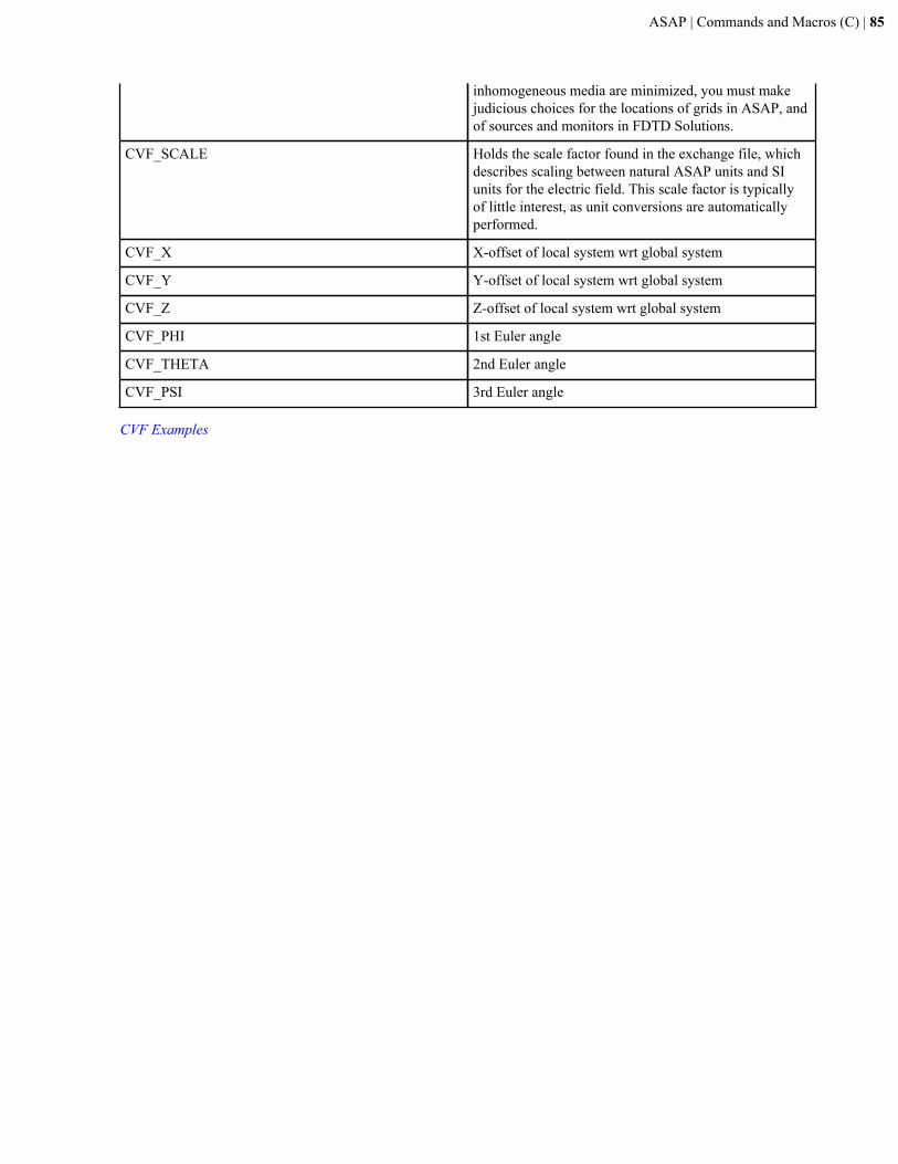
ASAP | Commands and Macros (C) | 85
inhomogeneous media are minimized, you must makejudicious choices for the locations of grids in ASAP, andof sources and monitors in FDTD Solutions.
CVF_SCALE Holds the scale factor found in the exchange file, whichdescribes scaling between natural ASAP units and SIunits for the electric field. This scale factor is typicallyof little interest, as unit conversions are automaticallyperformed.
CVF_X X-offset of local system wrt global system
CVF_Y Y-offset of local system wrt global system
CVF_Z Z-offset of local system wrt global system
CVF_PHI 1st Euler angle
CVF_THETA 2nd Euler angle
CVF_PSI 3rd Euler angle
CVF Examples
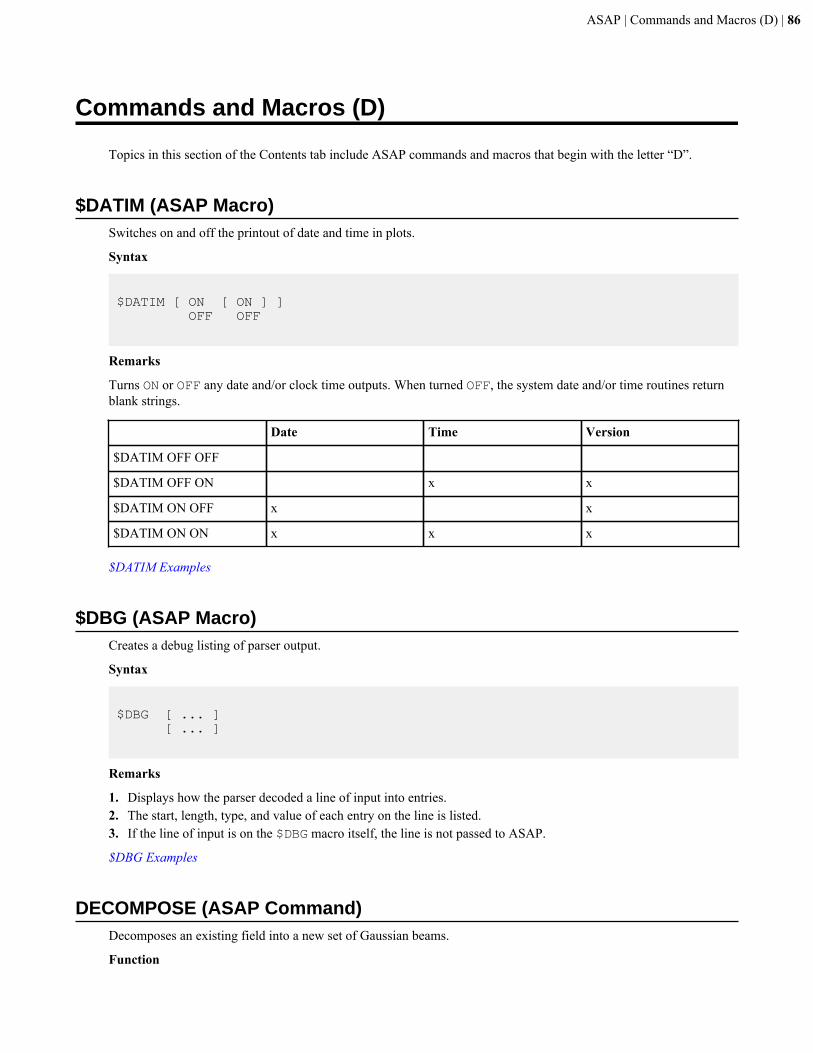
ASAP | Commands and Macros (D) | 86
Commands and Macros (D)
Topics in this section of the Contents tab include ASAP commands and macros that begin with the letter “D”.
$DATIM (ASAP Macro)Switches on and off the printout of date and time in plots.
Syntax
$DATIM [ ON [ ON ] ] OFF OFF
Remarks
Turns ON or OFF any date and/or clock time outputs. When turned OFF, the system date and/or time routines returnblank strings.
Date Time Version
$DATIM OFF OFF
$DATIM OFF ON x x
$DATIM ON OFF x x
$DATIM ON ON x x x
$DATIM Examples
$DBG (ASAP Macro)Creates a debug listing of parser output.
Syntax
$DBG [ ... ] [ ... ]
Remarks
1. Displays how the parser decoded a line of input into entries.2. The start, length, type, and value of each entry on the line is listed.3. If the line of input is on the $DBG macro itself, the line is not passed to ASAP.
$DBG Examples
DECOMPOSE (ASAP Command)Decomposes an existing field into a new set of Gaussian beams.
Function
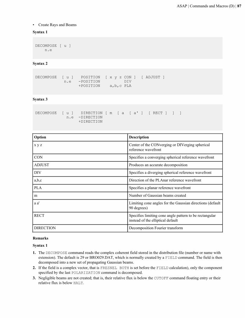
ASAP | Commands and Macros (D) | 87
• Create Rays and Beams
Syntax 1
DECOMPOSE [ u ] n.e
Syntax 2
DECOMPOSE [ u ] POSITION [ x y z CON ] [ ADJUST ] n.e -POSITION DIV +POSITION a,b,c PLA
Syntax 3
DECOMPOSE [ u ] DIRECTION [ m [ a [ a' ] [ RECT ] ] ] n.e -DIRECTION +DIRECTION
Option Description
x y z Center of the CONverging or DIVerging sphericalreference wavefront
CON Specifies a converging spherical reference wavefront
ADJUST Produces an accurate decomposition
DIV Specifies a diverging spherical reference wavefront
a,b,c Direction of the PLAnar reference wavefront
PLA Specifies a planar reference wavefront
m Number of Gaussian beams created
a a' Limiting cone angles for the Gaussian directions (default90 degrees)
RECT Specifies limiting cone angle pattern to be rectangularinstead of the elliptical default
DIRECTION Decomposition Fourier transform
Remarks
Syntax 1
1. The DECOMPOSE command reads the complex coherent field stored in the distribution file (number or name withextension). The default is 29 or BRO029.DAT, which is normally created by a FIELD command. The field is thendecomposed into a new set of propagating Gaussian beams.
2. If the field is a complex vector, that is FRESNEL BOTH is set before the FIELD calculation), only the componentspecified by the last POLARIZATION command is decomposed.
3. Negligible beams are not created; that is, their relative flux is below the CUTOFF command floating entry or theirrelative flux is below HALT.
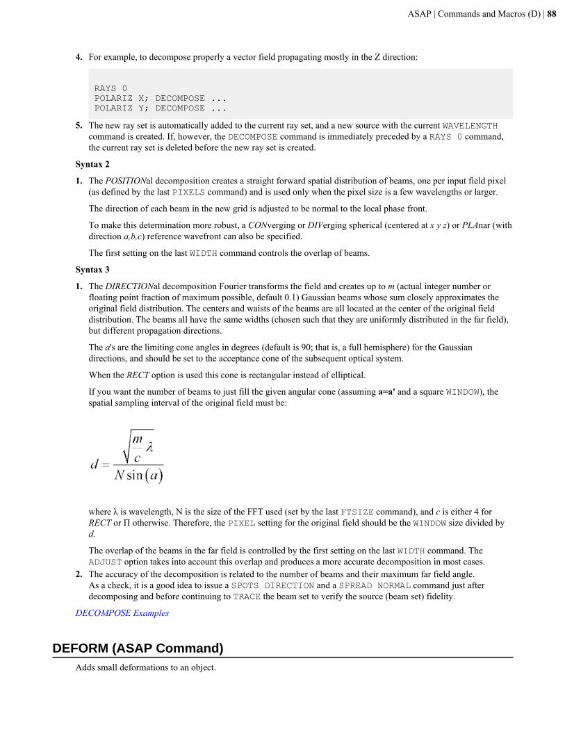
ASAP | Commands and Macros (D) | 88
4. For example, to decompose properly a vector field propagating mostly in the Z direction:
RAYS 0POLARIZ X; DECOMPOSE ...POLARIZ Y; DECOMPOSE ...
5. The new ray set is automatically added to the current ray set, and a new source with the current WAVELENGTHcommand is created. If, however, the DECOMPOSE command is immediately preceded by a RAYS 0 command,the current ray set is deleted before the new ray set is created.
Syntax 2
1. The POSITIONal decomposition creates a straight forward spatial distribution of beams, one per input field pixel(as defined by the last PIXELS command) and is used only when the pixel size is a few wavelengths or larger.
The direction of each beam in the new grid is adjusted to be normal to the local phase front.
To make this determination more robust, a CONverging or DIVerging spherical (centered at x y z) or PLAnar (withdirection a,b,c) reference wavefront can also be specified.
The first setting on the last WIDTH command controls the overlap of beams.
Syntax 3
1. The DIRECTIONal decomposition Fourier transforms the field and creates up to m (actual integer number orfloating point fraction of maximum possible, default 0.1) Gaussian beams whose sum closely approximates theoriginal field distribution. The centers and waists of the beams are all located at the center of the original fielddistribution. The beams all have the same widths (chosen such that they are uniformly distributed in the far field),but different propagation directions.
The a's are the limiting cone angles in degrees (default is 90; that is, a full hemisphere) for the Gaussiandirections, and should be set to the acceptance cone of the subsequent optical system.
When the RECT option is used this cone is rectangular instead of elliptical.
If you want the number of beams to just fill the given angular cone (assuming a=a' and a square WINDOW), thespatial sampling interval of the original field must be:
where λ is wavelength, N is the size of the FFT used (set by the last FTSIZE command), and c is either 4 forRECT or Π otherwise. Therefore, the PIXEL setting for the original field should be the WINDOW size divided byd.
The overlap of the beams in the far field is controlled by the first setting on the last WIDTH command. TheADJUST option takes into account this overlap and produces a more accurate decomposition in most cases.
2. The accuracy of the decomposition is related to the number of beams and their maximum far field angle.As a check, it is a good idea to issue a SPOTS DIRECTION and a SPREAD NORMAL command just afterdecomposing and before continuing to TRACE the beam set to verify the source (beam set) fidelity.
DECOMPOSE Examples
DEFORM (ASAP Command)Adds small deformations to an object.
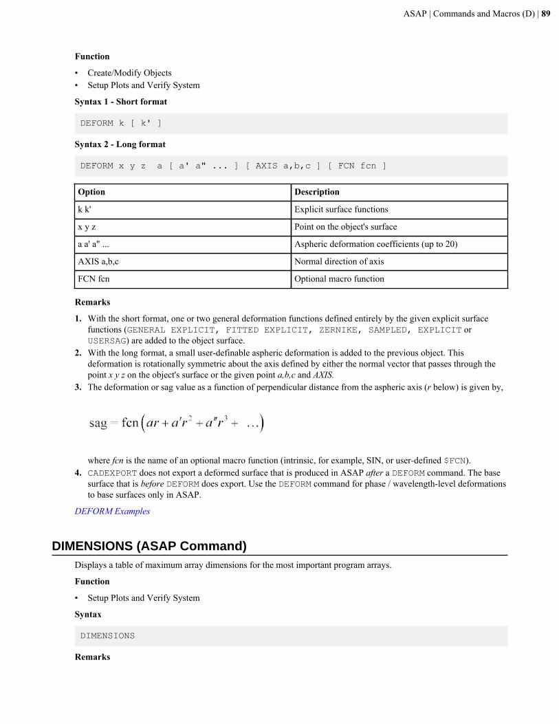
ASAP | Commands and Macros (D) | 89
Function
• Create/Modify Objects• Setup Plots and Verify System
Syntax 1 - Short format
DEFORM k [ k' ]
Syntax 2 - Long format
DEFORM x y z a [ a' a" ... ] [ AXIS a,b,c ] [ FCN fcn ]
Option Description
k k' Explicit surface functions
x y z Point on the object's surface
a a' a" ... Aspheric deformation coefficients (up to 20)
AXIS a,b,c Normal direction of axis
FCN fcn Optional macro function
Remarks
1. With the short format, one or two general deformation functions defined entirely by the given explicit surfacefunctions (GENERAL EXPLICIT, FITTED EXPLICIT, ZERNIKE, SAMPLED, EXPLICIT orUSERSAG) are added to the object surface.
2. With the long format, a small user-definable aspheric deformation is added to the previous object. Thisdeformation is rotationally symmetric about the axis defined by either the normal vector that passes through thepoint x y z on the object's surface or the given point a,b,c and AXIS.
3. The deformation or sag value as a function of perpendicular distance from the aspheric axis (r below) is given by,
where fcn is the name of an optional macro function (intrinsic, for example, SIN, or user-defined $FCN).4. CADEXPORT does not export a deformed surface that is produced in ASAP after a DEFORM command. The base
surface that is before DEFORM does export. Use the DEFORM command for phase / wavelength-level deformationsto base surfaces only in ASAP.
DEFORM Examples
DIMENSIONS (ASAP Command)Displays a table of maximum array dimensions for the most important program arrays.
Function
• Setup Plots and Verify System
Syntax
DIMENSIONS
Remarks
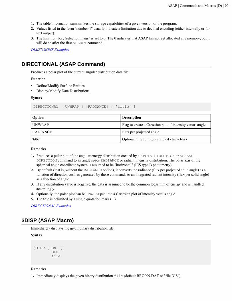
ASAP | Commands and Macros (D) | 90
1. The table information summarizes the storage capabilities of a given version of the program.2. Values listed in the form "number-1" usually indicate a limitation due to decimal encoding (either internally or for
text output).3. The limit for "Ray Selection Flags" is set to 0. The 0 indicates that ASAP has not yet allocated any memory, but it
will do so after the first SELECT command.
DIMENSIONS Examples
DIRECTIONAL (ASAP Command)Produces a polar plot of the current angular distribution data file.
Function
• Define/Modify Surfunc Entities• Display/Modify Data Distributions
Syntax
DIRECTIONAL [ UNWRAP ] [RADIANCE] [ 'title' ]
Option Description
UNWRAP Flag to create a Cartesian plot of intensity versus angle
RADIANCE Flux per projected angle
'title' Optional title for plot (up to 64 characters)
Remarks
1. Produces a polar plot of the angular energy distribution created by a SPOTS DIRECTION or SPREADDIRECTION command to an angle space RADIANCE or radiant intensity distribution. The polar axis of thespherical angle coordinate system is assumed to be "horizontal" (IES type B photometry).
2. By default (that is, without the RADIANCE option), it converts the radiance (flux per projected solid angle) as afunction of direction cosines generated by these commands to an integrated radiant intensity (flux per solid angle)as a function of angle.
3. If any distribution value is negative, the data is assumed to be the common logarithm of energy and is handledaccordingly.
4. Optionally, the polar plot can be UNWRAPped into a Cartesian plot of intensity versus angle.5. The title is delimited by a single quotation mark ( ' ).
DIRECTIONAL Examples
$DISP (ASAP Macro)Immediately displays the given binary distribution file.
Syntax
$DISP [ ON ] OFF file
Remarks
1. Immediately displays the given binary distribution file (default BRO009.DAT or "file.DIS").
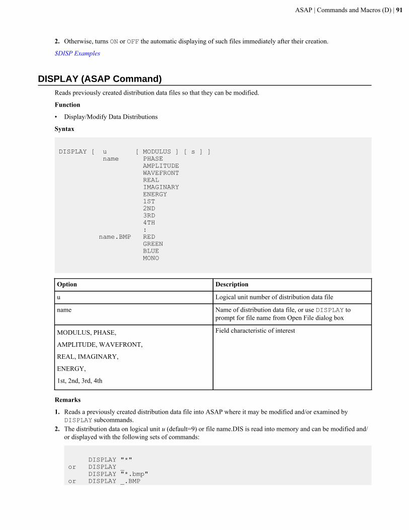
ASAP | Commands and Macros (D) | 91
2. Otherwise, turns ON or OFF the automatic displaying of such files immediately after their creation.
$DISP Examples
DISPLAY (ASAP Command)Reads previously created distribution data files so that they can be modified.
Function
• Display/Modify Data Distributions
Syntax
DISPLAY [ u [ MODULUS ] [ s ] ] name PHASE AMPLITUDE WAVEFRONT REAL IMAGINARY ENERGY 1ST 2ND 3RD 4TH : name.BMP RED GREEN BLUE MONO
Option Description
u Logical unit number of distribution data file
name Name of distribution data file, or use DISPLAY toprompt for file name from Open File dialog box
MODULUS, PHASE,
AMPLITUDE, WAVEFRONT,
REAL, IMAGINARY,
ENERGY,
1st, 2nd, 3rd, 4th
Field characteristic of interest
Remarks
1. Reads a previously created distribution data file into ASAP where it may be modified and/or examined byDISPLAY subcommands.
2. The distribution data on logical unit u (default=9) or file name.DIS is read into memory and can be modified and/or displayed with the following sets of commands:
DISPLAY "*"or DISPLAY _ DISPLAY "*.bmp"or DISPLAY _.BMP
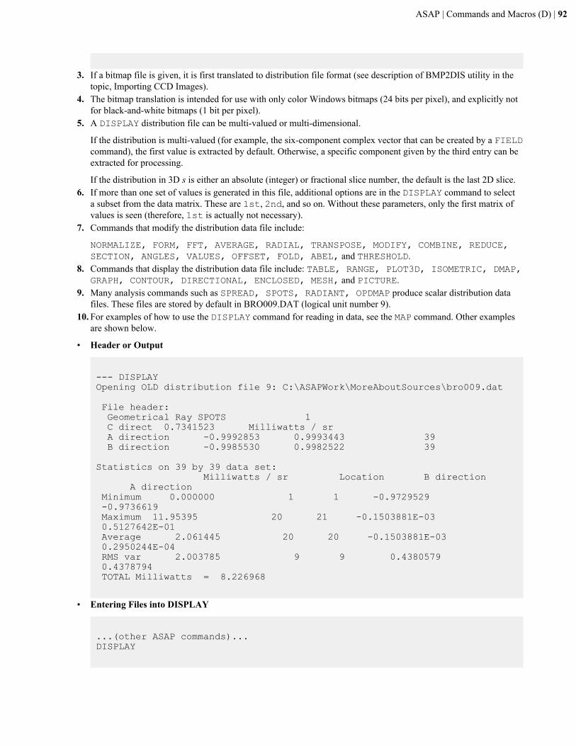
ASAP | Commands and Macros (D) | 92
3. If a bitmap file is given, it is first translated to distribution file format (see description of BMP2DIS utility in thetopic, Importing CCD Images).
4. The bitmap translation is intended for use with only color Windows bitmaps (24 bits per pixel), and explicitly notfor black-and-white bitmaps (1 bit per pixel).
5. A DISPLAY distribution file can be multi-valued or multi-dimensional.
If the distribution is multi-valued (for example, the six-component complex vector that can be created by a FIELDcommand), the first value is extracted by default. Otherwise, a specific component given by the third entry can beextracted for processing.
If the distribution in 3D s is either an absolute (integer) or fractional slice number, the default is the last 2D slice.6. If more than one set of values is generated in this file, additional options are in the DISPLAY command to select
a subset from the data matrix. These are 1st, 2nd, and so on. Without these parameters, only the first matrix ofvalues is seen (therefore, 1st is actually not necessary).
7. Commands that modify the distribution data file include:
NORMALIZE, FORM, FFT, AVERAGE, RADIAL, TRANSPOSE, MODIFY, COMBINE, REDUCE,SECTION, ANGLES, VALUES, OFFSET, FOLD, ABEL, and THRESHOLD.
8. Commands that display the distribution data file include: TABLE, RANGE, PLOT3D, ISOMETRIC, DMAP,GRAPH, CONTOUR, DIRECTIONAL, ENCLOSED, MESH, and PICTURE.
9. Many analysis commands such as SPREAD, SPOTS, RADIANT, OPDMAP produce scalar distribution datafiles. These files are stored by default in BRO009.DAT (logical unit number 9).
10. For examples of how to use the DISPLAY command for reading in data, see the MAP command. Other examplesare shown below.
• Header or Output
--- DISPLAYOpening OLD distribution file 9: C:\ASAPWork\MoreAboutSources\bro009.dat
File header: Geometrical Ray SPOTS 1 C direct 0.7341523 Milliwatts / sr A direction -0.9992853 0.9993443 39 B direction -0.9985530 0.9982522 39
Statistics on 39 by 39 data set: Milliwatts / sr Location B direction A direction Minimum 0.000000 1 1 -0.9729529 -0.9736619 Maximum 11.95395 20 21 -0.1503881E-03 0.5127642E-01 Average 2.061445 20 20 -0.1503881E-03 0.2950244E-04 RMS var 2.003785 9 9 0.4380579 0.4378794 TOTAL Milliwatts = 8.226968
• Entering Files into DISPLAY
...(other ASAP commands)...DISPLAY
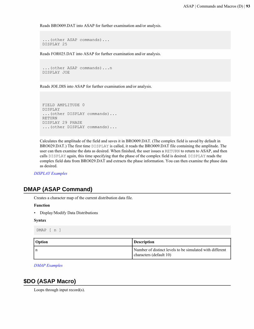
ASAP | Commands and Macros (D) | 93
Reads BRO009.DAT into ASAP for further examination and/or analysis.
...(other ASAP commands)...DISPLAY 25
Reads FOR025.DAT into ASAP for further examination and/or analysis.
...(other ASAP commands)...nDISPLAY JOE
Reads JOE.DIS into ASAP for further examination and/or analysis.
FIELD AMPLITUDE 0DISPLAY...(other DISPLAY commands)...RETURNDISPLAY 29 PHASE...(other DISPLAY commands)...
Calculates the amplitude of the field and saves it in BRO009.DAT. (The complex field is saved by default inBRO029.DAT.) The first time DISPLAY is called, it reads the BRO009.DAT file containing the amplitude. Theuser can then examine the data as desired. When finished, the user issues a RETURN to return to ASAP, and thencalls DISPLAY again, this time specifying that the phase of the complex field is desired. DISPLAY reads thecomplex field data from BRO029.DAT and extracts the phase information. You can then examine the phase dataas desired.
DISPLAY Examples
DMAP (ASAP Command)Creates a character map of the current distribution data file.
Function
• Display/Modify Data Distributions
Syntax
DMAP [ n ]
Option Description
n Number of distinct levels to be simulated with differentcharacters (default 10)
DMAP Examples
$DO (ASAP Macro)Loops through input record(s).
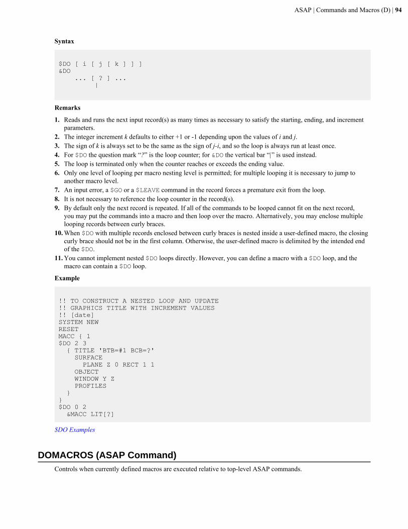
ASAP | Commands and Macros (D) | 94
Syntax
$DO [ i [ j [ k ] ] ]&DO ... [ ? ] ... |
Remarks
1. Reads and runs the next input record(s) as many times as necessary to satisfy the starting, ending, and incrementparameters.
2. The integer increment k defaults to either +1 or -1 depending upon the values of i and j.3. The sign of k is always set to be the same as the sign of j-i, and so the loop is always run at least once.4. For $DO the question mark “?” is the loop counter; for &DO the vertical bar “|” is used instead.5. The loop is terminated only when the counter reaches or exceeds the ending value.6. Only one level of looping per macro nesting level is permitted; for multiple looping it is necessary to jump to
another macro level.7. An input error, a $GO or a $LEAVE command in the record forces a premature exit from the loop.8. It is not necessary to reference the loop counter in the record(s).9. By default only the next record is repeated. If all of the commands to be looped cannot fit on the next record,
you may put the commands into a macro and then loop over the macro. Alternatively, you may enclose multiplelooping records between curly braces.
10. When $DO with multiple records enclosed between curly braces is nested inside a user-defined macro, the closingcurly brace should not be in the first column. Otherwise, the user-defined macro is delimited by the intended endof the $DO.
11. You cannot implement nested $DO loops directly. However, you can define a macro with a $DO loop, and themacro can contain a $DO loop.
Example
!! TO CONSTRUCT A NESTED LOOP AND UPDATE !! GRAPHICS TITLE WITH INCREMENT VALUES!! [date]SYSTEM NEWRESETMACC { 1$DO 2 3 { TITLE 'BTB=#1 BCB=?' SURFACE PLANE Z 0 RECT 1 1 OBJECT WINDOW Y Z PROFILES } } $DO 0 2 &MACC LIT[?]
$DO Examples
DOMACROS (ASAP Command)Controls when currently defined macros are executed relative to top-level ASAP commands.
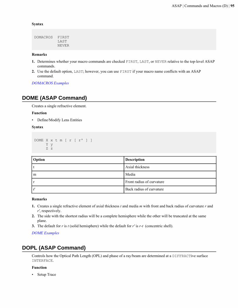
ASAP | Commands and Macros (D) | 95
Syntax
DOMACROS FIRST LAST NEVER
Remarks
1. Determines whether your macro commands are checked FIRST, LAST, or NEVER relative to the top-level ASAPcommands.
2. Use the default option, LAST; however, you can use FIRST if your macro name conflicts with an ASAPcommand.
DOMACROS Examples
DOME (ASAP Command)Creates a single refractive element.
Function
• Define/Modify Lens Entities
Syntax
DOME X x t m [ r [ r' ] ] Y y Z z
Option Description
t Axial thickness
m Media
r Front radius of curvature
r' Back radius of curvature
Remarks
1. Creates a single refractive element of axial thickness t and media m with front and back radius of curvature r andr', respectively.
2. The side with the shortest radius will be a complete hemisphere while the other will be truncated at the sameplane.
3. The default for r is t (solid hemisphere) while the default for r' is r-t (concentric shell).
DOME Examples
DOPL (ASAP Command)Controls how the Optical Path Length (OPL) and phase of a ray/beam are determined at a DIFFRACTive surfaceINTERFACE.
Function
• Setup Trace
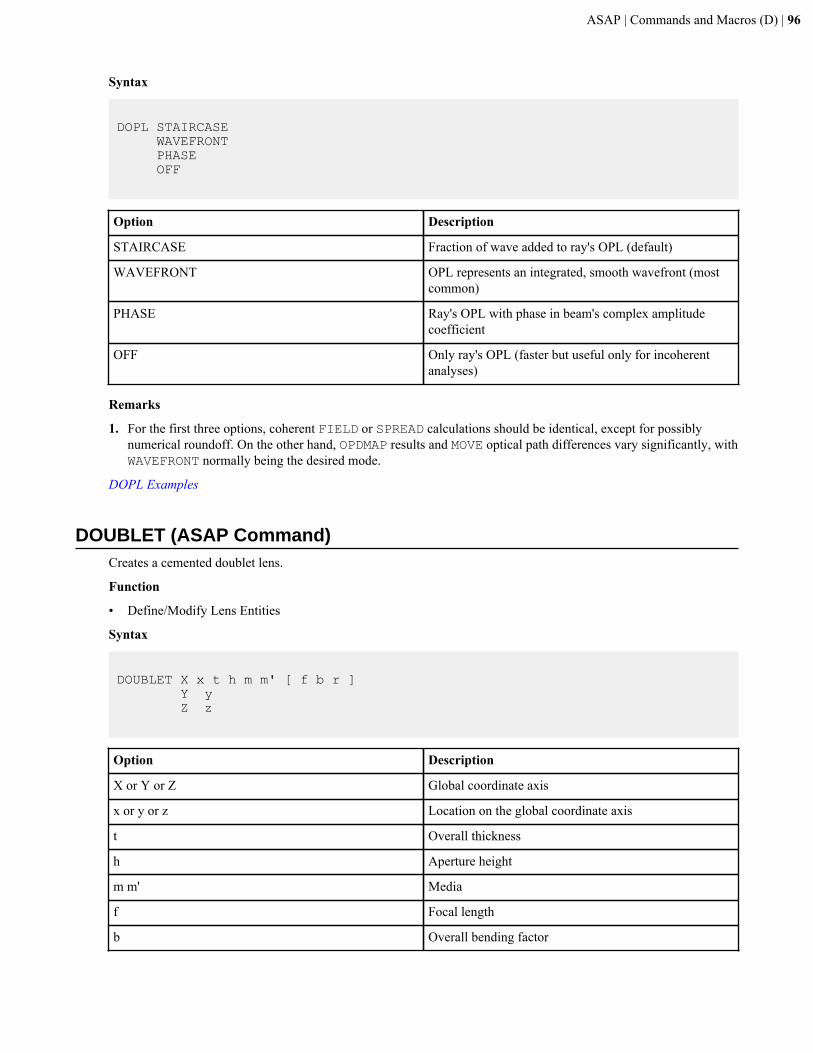
ASAP | Commands and Macros (D) | 96
Syntax
DOPL STAIRCASE WAVEFRONT PHASE OFF
Option Description
STAIRCASE Fraction of wave added to ray's OPL (default)
WAVEFRONT OPL represents an integrated, smooth wavefront (mostcommon)
PHASE Ray's OPL with phase in beam's complex amplitudecoefficient
OFF Only ray's OPL (faster but useful only for incoherentanalyses)
Remarks
1. For the first three options, coherent FIELD or SPREAD calculations should be identical, except for possiblynumerical roundoff. On the other hand, OPDMAP results and MOVE optical path differences vary significantly, withWAVEFRONT normally being the desired mode.
DOPL Examples
DOUBLET (ASAP Command)Creates a cemented doublet lens.
Function
• Define/Modify Lens Entities
Syntax
DOUBLET X x t h m m' [ f b r ] Y y Z z
Option Description
X or Y or Z Global coordinate axis
x or y or z Location on the global coordinate axis
t Overall thickness
h Aperture height
m m' Media
f Focal length
b Overall bending factor
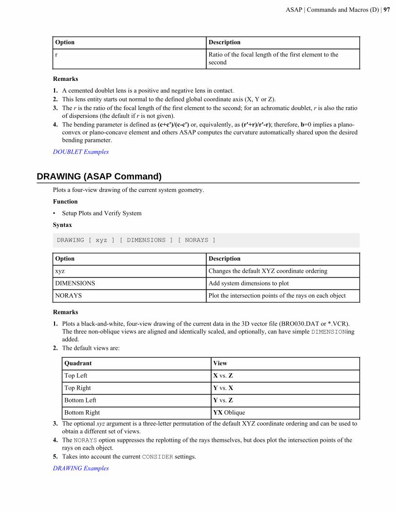
ASAP | Commands and Macros (D) | 97
Option Description
r Ratio of the focal length of the first element to thesecond
Remarks
1. A cemented doublet lens is a positive and negative lens in contact.2. This lens entity starts out normal to the defined global coordinate axis (X, Y or Z).3. The r is the ratio of the focal length of the first element to the second; for an achromatic doublet, r is also the ratio
of dispersions (the default if r is not given).4. The bending parameter is defined as (c+c')/(c-c') or, equivalently, as (r'+r)/r'-r); therefore, b=0 implies a plano-
convex or plano-concave element and others ASAP computes the curvature automatically shared upon the desiredbending parameter.
DOUBLET Examples
DRAWING (ASAP Command)Plots a four-view drawing of the current system geometry.
Function
• Setup Plots and Verify System
Syntax
DRAWING [ xyz ] [ DIMENSIONS ] [ NORAYS ]
Option Description
xyz Changes the default XYZ coordinate ordering
DIMENSIONS Add system dimensions to plot
NORAYS Plot the intersection points of the rays on each object
Remarks
1. Plots a black-and-white, four-view drawing of the current data in the 3D vector file (BRO030.DAT or *.VCR).The three non-oblique views are aligned and identically scaled, and optionally, can have simple DIMENSIONingadded.
2. The default views are:
Quadrant View
Top Left X vs. Z
Top Right Y vs. X
Bottom Left Y vs. Z
Bottom Right YX Oblique
3. The optional xyz argument is a three-letter permutation of the default XYZ coordinate ordering and can be used toobtain a different set of views.
4. The NORAYS option suppresses the replotting of the rays themselves, but does plot the intersection points of therays on each object.
5. Takes into account the current CONSIDER settings.
DRAWING Examples
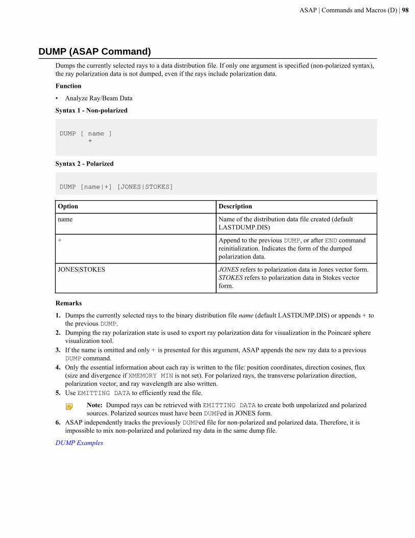
ASAP | Commands and Macros (D) | 98
DUMP (ASAP Command)Dumps the currently selected rays to a data distribution file. If only one argument is specified (non-polarized syntax),the ray polarization data is not dumped, even if the rays include polarization data.
Function
• Analyze Ray/Beam Data
Syntax 1 - Non-polarized
DUMP [ name ] +
Syntax 2 - Polarized
DUMP [name|+] [JONES|STOKES]
Option Description
name Name of the distribution data file created (defaultLASTDUMP.DIS)
+ Append to the previous DUMP, or after END commandreinitialization. Indicates the form of the dumpedpolarization data.
JONES|STOKES JONES refers to polarization data in Jones vector form.STOKES refers to polarization data in Stokes vectorform.
Remarks
1. Dumps the currently selected rays to the binary distribution file name (default LASTDUMP.DIS) or appends + tothe previous DUMP.
2. Dumping the ray polarization state is used to export ray polarization data for visualization in the Poincaré spherevisualization tool.
3. If the name is omitted and only + is presented for this argument, ASAP appends the new ray data to a previousDUMP command.
4. Only the essential information about each ray is written to the file: position coordinates, direction cosines, flux(size and divergence if XMEMORY MIN is not set). For polarized rays, the transverse polarization direction,polarization vector, and ray wavelength are also written.
5. Use EMITTING DATA to efficiently read the file.
Note: Dumped rays can be retrieved with EMITTING DATA to create both unpolarized and polarizedsources. Polarized sources must have been DUMPed in JONES form.
6. ASAP independently tracks the previously DUMPed file for non-polarized and polarized data. Therefore, it isimpossible to mix non-polarized and polarized ray data in the same dump file.
DUMP Examples
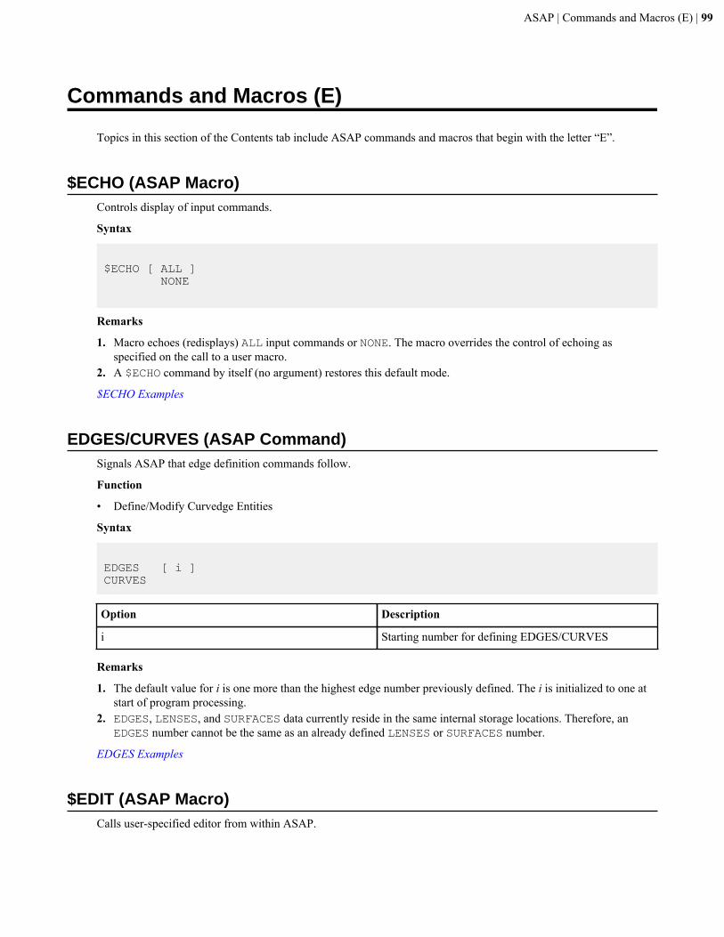
ASAP | Commands and Macros (E) | 99
Commands and Macros (E)
Topics in this section of the Contents tab include ASAP commands and macros that begin with the letter “E”.
$ECHO (ASAP Macro)Controls display of input commands.
Syntax
$ECHO [ ALL ] NONE
Remarks
1. Macro echoes (redisplays) ALL input commands or NONE. The macro overrides the control of echoing asspecified on the call to a user macro.
2. A $ECHO command by itself (no argument) restores this default mode.
$ECHO Examples
EDGES/CURVES (ASAP Command)Signals ASAP that edge definition commands follow.
Function
• Define/Modify Curvedge Entities
Syntax
EDGES [ i ]CURVES
Option Description
i Starting number for defining EDGES/CURVES
Remarks
1. The default value for i is one more than the highest edge number previously defined. The i is initialized to one atstart of program processing.
2. EDGES, LENSES, and SURFACES data currently reside in the same internal storage locations. Therefore, anEDGES number cannot be the same as an already defined LENSES or SURFACES number.
EDGES Examples
$EDIT (ASAP Macro)Calls user-specified editor from within ASAP.
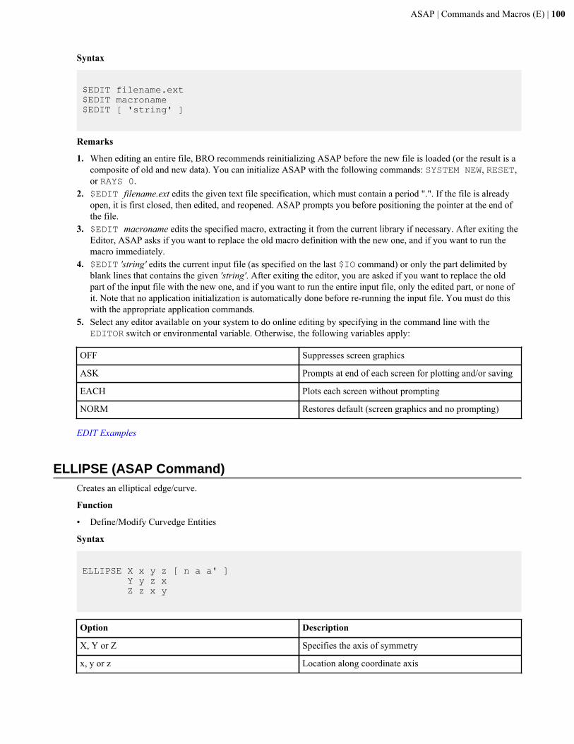
ASAP | Commands and Macros (E) | 100
Syntax
$EDIT filename.ext$EDIT macroname$EDIT [ 'string' ]
Remarks
1. When editing an entire file, BRO recommends reinitializing ASAP before the new file is loaded (or the result is acomposite of old and new data). You can initialize ASAP with the following commands: SYSTEM NEW, RESET,or RAYS 0.
2. $EDIT filename.ext edits the given text file specification, which must contain a period ".". If the file is alreadyopen, it is first closed, then edited, and reopened. ASAP prompts you before positioning the pointer at the end ofthe file.
3. $EDIT macroname edits the specified macro, extracting it from the current library if necessary. After exiting theEditor, ASAP asks if you want to replace the old macro definition with the new one, and if you want to run themacro immediately.
4. $EDIT 'string' edits the current input file (as specified on the last $IO command) or only the part delimited byblank lines that contains the given 'string'. After exiting the editor, you are asked if you want to replace the oldpart of the input file with the new one, and if you want to run the entire input file, only the edited part, or none ofit. Note that no application initialization is automatically done before re-running the input file. You must do thiswith the appropriate application commands.
5. Select any editor available on your system to do online editing by specifying in the command line with theEDITOR switch or environmental variable. Otherwise, the following variables apply:
OFF Suppresses screen graphics
ASK Prompts at end of each screen for plotting and/or saving
EACH Plots each screen without prompting
NORM Restores default (screen graphics and no prompting)
EDIT Examples
ELLIPSE (ASAP Command)Creates an elliptical edge/curve.
Function
• Define/Modify Curvedge Entities
Syntax
ELLIPSE X x y z [ n a a' ] Y y z x Z z x y
Option Description
X, Y or Z Specifies the axis of symmetry
x, y or z Location along coordinate axis
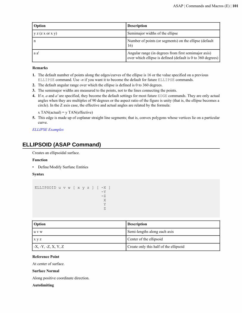
ASAP | Commands and Macros (E) | 101
Option Description
y z (z x or x y) Semimajor widths of the ellipse
n Number of points (or segments) on the ellipse (default16)
a a' Angular range (in degrees from first semimajor axis)over which ellipse is defined (default is 0 to 360 degrees)
Remarks
1. The default number of points along the edges/curves of the ellipse is 16 or the value specified on a previousELLIPSE command. Use -n if you want it to become the default for future ELLIPSE commands.
2. The default angular range over which the ellipse is defined is 0 to 360 degrees.3. The semimajor widths are measured to the points, not to the lines connecting the points.4. If n, a and a' are specified, they become the default settings for most future EDGE commands. They are only actual
angles when they are multiples of 90 degrees or the aspect ratio of the figure is unity (that is, the ellipse becomes acircle). In the Z axis case, the effective and actual angles are related by the formula:
x TAN(actual) = y TAN(effective)5. This edge is made up of coplanar straight line segments; that is, convex polygons whose vertices lie on a particular
curve.
ELLIPSE Examples
ELLIPSOID (ASAP Command)Creates an ellipsoidal surface.
Function
• Define/Modify Surfunc Entities
Syntax
ELLIPSOID u v w [ x y z ] [ -X ] -Y -Z X Y Z
Option Description
u v w Semi-lengths along each axis
x y z Center of the ellipsoid
-X, -Y, -Z, X, Y, Z Create only this half of the ellipsoid
Reference Point
At center of surface.
Surface Normal
Along positive coordinate direction.
Autolimiting
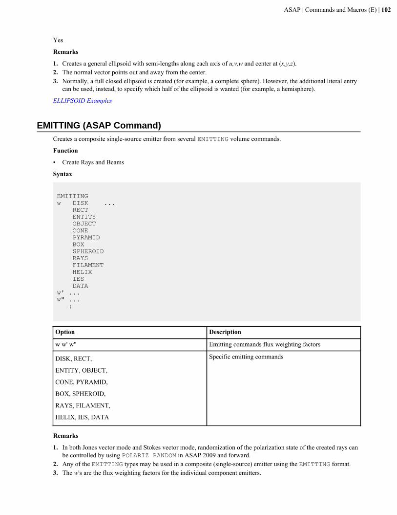
ASAP | Commands and Macros (E) | 102
Yes
Remarks
1. Creates a general ellipsoid with semi-lengths along each axis of u,v,w and center at (x,y,z).2. The normal vector points out and away from the center.3. Normally, a full closed ellipsoid is created (for example, a complete sphere). However, the additional literal entry
can be used, instead, to specify which half of the ellipsoid is wanted (for example, a hemisphere).
ELLIPSOID Examples
EMITTING (ASAP Command)Creates a composite single-source emitter from several EMITTING volume commands.
Function
• Create Rays and Beams
Syntax
EMITTINGw DISK ... RECT ENTITY OBJECT CONE PYRAMID BOX SPHEROID RAYS FILAMENT HELIX IES DATAw' ...w" ... :
Option Description
w w' w" Emitting commands flux weighting factors
DISK, RECT,
ENTITY, OBJECT,
CONE, PYRAMID,
BOX, SPHEROID,
RAYS, FILAMENT,
HELIX, IES, DATA
Specific emitting commands
Remarks
1. In both Jones vector mode and Stokes vector mode, randomization of the polarization state of the created rays canbe controlled by using POLARIZ RANDOM in ASAP 2009 and forward.
2. Any of the EMITTING types may be used in a composite (single-source) emitter using the EMITTING format.3. The w's are the flux weighting factors for the individual component emitters.
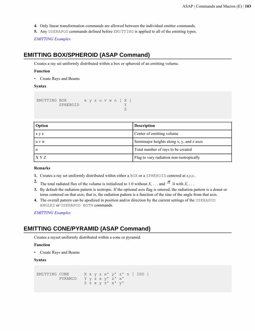
ASAP | Commands and Macros (E) | 103
4. Only linear transformation commands are allowed between the individual emitter commands.5. Any USERAPOD commands defined before EMITTING is applied to all of the emitting types.
EMITTING Examples
EMITTING BOX/SPHEROID (ASAP Command)Creates a ray set uniformly distributed within a box or spheroid of an emitting volume.
Function
• Create Rays and Beams
Syntax
EMITTING BOX x y z u v w n [ X ] SPHEROID Y Z
Option Description
x y z Center of emitting volume
u v w Semimajor heights along x, y, and z axes
n Total number of rays to be created
X Y Z Flag to vary radiation non-isotropically
Remarks
1. Creates a ray set uniformly distributed within either a BOX or a SPHEROID centered at x,y,z..2. The total radiated flux of the volume is initialized to 1.0 without X, . . . and /4 with X, . . .3. By default the radiation pattern is isotropic. If the optional axis flag is entered, the radiation pattern is a donut or
torus centered on that axis; that is, the radiation pattern is a function of the sine of the angle from that axis.4. The overall pattern can be apodized in position and/or direction by the current settings of the USERAPOD
ANGLES or USERAPOD BOTH commands.
EMITTING Examples
EMITTING CONE/PYRAMID (ASAP Command)Creates a rayset uniformly distributed within a cone or pyramid.
Function
• Create Rays and Beams
Syntax
EMITTING CONE X x y z x' y' z' n [ ISO ] PYRAMID Y y z x y' z' x' Z z x y z' x' y'
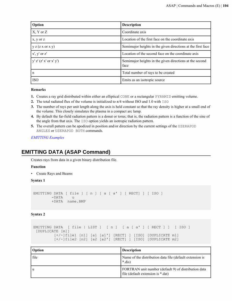
ASAP | Commands and Macros (E) | 104
Option Description
X, Y or Z Coordinate axis
x, y or z Location of the first face on the coordinate axis
y z (z x or x y) Semimajor heights in the given directions at the first face
x', y' or z' Location of the second face on the coordinate axis
y' z' (z' x' or x' y') Semimajor heights in the given directions at the secondface
n Total number of rays to be created
ISO Emits as an isotropic source
Remarks
1. Creates a ray grid distributed within either an elliptical CONE or a rectangular PYRAMID emitting volume.2. The total radiated flux of the volume is initialized to π/4 without ISO and 1.0 with ISO3. The number of rays per unit length along the axis is held constant so that the ray density is higher at a small end of
the volume. This closely simulates the plasma in a compact arc lamp.4. By default the far-field radiation pattern is a donut or torus; that is, the radiation pattern is a function of the sine of
the angle from that axis. The ISO option yields an isotropic radiation pattern.5. The overall pattern can be apodized in position and/or direction by the current settings of the USERAPOD
ANGLES or USERAPOD BOTH commands.
EMITTING Examples
EMITTING DATA (ASAP Command)Creates rays from data in a given binary distribution file.
Function
• Create Rays and Beams
Syntax 1
EMITTING DATA [ file ] [ n ] [ a [ a' ] [ RECT] ] [ ISO ] -DATA u +DATA name.BMP
Syntax 2
EMITTING DATA [ file | LIST ] [ n ] [ a [ a' ] [ RECT ] ] [ ISO ] [DUPLICATE [m]] [+/-]file1 [n1] [a1 [a1'] [RECT] ] [ISO] [DUPLICATE m1] [+/-]file2 [n2] [a2 [a2'] [RECT] ] [ISO] [DUPLICATE m2]
Option Description
file Name of the distribution data file (default extension is*.dis)
u FORTRAN unit number (default 9) of distribution datafile (default extension is *.dat)
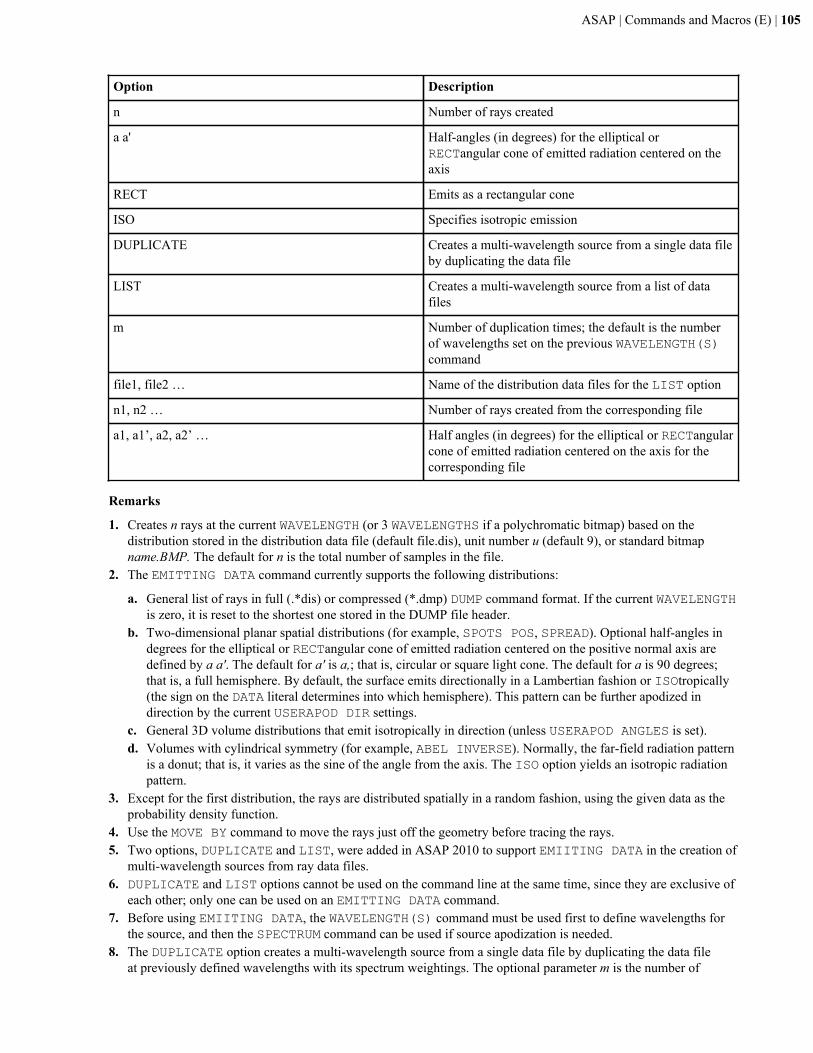
ASAP | Commands and Macros (E) | 105
Option Description
n Number of rays created
a a' Half-angles (in degrees) for the elliptical orRECTangular cone of emitted radiation centered on theaxis
RECT Emits as a rectangular cone
ISO Specifies isotropic emission
DUPLICATE Creates a multi-wavelength source from a single data fileby duplicating the data file
LIST Creates a multi-wavelength source from a list of datafiles
m Number of duplication times; the default is the numberof wavelengths set on the previous WAVELENGTH(S)command
file1, file2 … Name of the distribution data files for the LIST option
n1, n2 … Number of rays created from the corresponding file
a1, a1’, a2, a2’ … Half angles (in degrees) for the elliptical or RECTangularcone of emitted radiation centered on the axis for thecorresponding file
Remarks
1. Creates n rays at the current WAVELENGTH (or 3 WAVELENGTHS if a polychromatic bitmap) based on thedistribution stored in the distribution data file (default file.dis), unit number u (default 9), or standard bitmapname.BMP. The default for n is the total number of samples in the file.
2. The EMITTING DATA command currently supports the following distributions:
a. General list of rays in full (.*dis) or compressed (*.dmp) DUMP command format. If the current WAVELENGTHis zero, it is reset to the shortest one stored in the DUMP file header.
b. Two-dimensional planar spatial distributions (for example, SPOTS POS, SPREAD). Optional half-angles indegrees for the elliptical or RECTangular cone of emitted radiation centered on the positive normal axis aredefined by a a'. The default for a' is a,; that is, circular or square light cone. The default for a is 90 degrees;that is, a full hemisphere. By default, the surface emits directionally in a Lambertian fashion or ISOtropically(the sign on the DATA literal determines into which hemisphere). This pattern can be further apodized indirection by the current USERAPOD DIR settings.
c. General 3D volume distributions that emit isotropically in direction (unless USERAPOD ANGLES is set).d. Volumes with cylindrical symmetry (for example, ABEL INVERSE). Normally, the far-field radiation pattern
is a donut; that is, it varies as the sine of the angle from the axis. The ISO option yields an isotropic radiationpattern.
3. Except for the first distribution, the rays are distributed spatially in a random fashion, using the given data as theprobability density function.
4. Use the MOVE BY command to move the rays just off the geometry before tracing the rays.5. Two options, DUPLICATE and LIST, were added in ASAP 2010 to support EMIITING DATA in the creation of
multi-wavelength sources from ray data files.6. DUPLICATE and LIST options cannot be used on the command line at the same time, since they are exclusive of
each other; only one can be used on an EMITTING DATA command.7. Before using EMIITING DATA, the WAVELENGTH(S) command must be used first to define wavelengths for
the source, and then the SPECTRUM command can be used if source apodization is needed.8. The DUPLICATE option creates a multi-wavelength source from a single data file by duplicating the data file
at previously defined wavelengths with its spectrum weightings. The optional parameter m is the number of
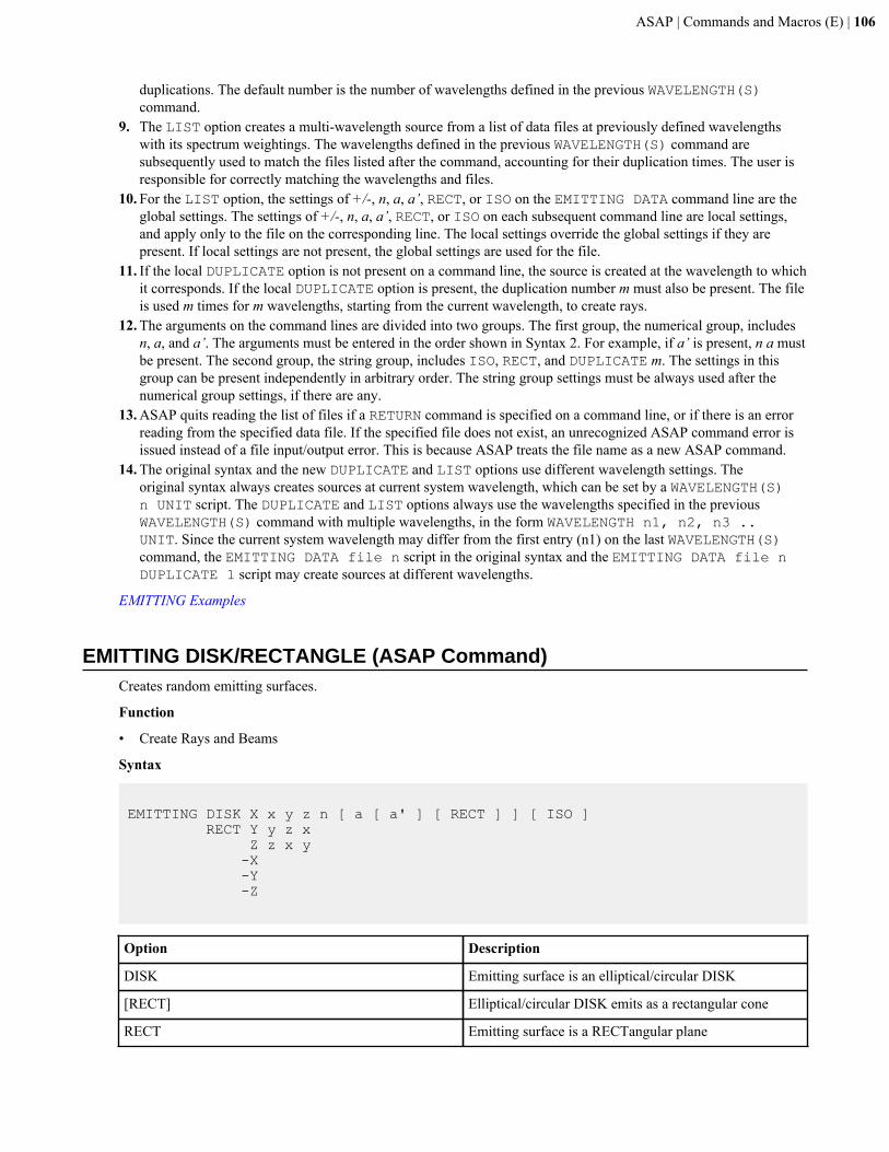
ASAP | Commands and Macros (E) | 106
duplications. The default number is the number of wavelengths defined in the previous WAVELENGTH(S)command.
9. The LIST option creates a multi-wavelength source from a list of data files at previously defined wavelengthswith its spectrum weightings. The wavelengths defined in the previous WAVELENGTH(S) command aresubsequently used to match the files listed after the command, accounting for their duplication times. The user isresponsible for correctly matching the wavelengths and files.
10. For the LIST option, the settings of +/-, n, a, a’, RECT, or ISO on the EMITTING DATA command line are theglobal settings. The settings of +/-, n, a, a’, RECT, or ISO on each subsequent command line are local settings,and apply only to the file on the corresponding line. The local settings override the global settings if they arepresent. If local settings are not present, the global settings are used for the file.
11. If the local DUPLICATE option is not present on a command line, the source is created at the wavelength to whichit corresponds. If the local DUPLICATE option is present, the duplication number m must also be present. The fileis used m times for m wavelengths, starting from the current wavelength, to create rays.
12. The arguments on the command lines are divided into two groups. The first group, the numerical group, includesn, a, and a’. The arguments must be entered in the order shown in Syntax 2. For example, if a’ is present, n a mustbe present. The second group, the string group, includes ISO, RECT, and DUPLICATE m. The settings in thisgroup can be present independently in arbitrary order. The string group settings must be always used after thenumerical group settings, if there are any.
13. ASAP quits reading the list of files if a RETURN command is specified on a command line, or if there is an errorreading from the specified data file. If the specified file does not exist, an unrecognized ASAP command error isissued instead of a file input/output error. This is because ASAP treats the file name as a new ASAP command.
14. The original syntax and the new DUPLICATE and LIST options use different wavelength settings. Theoriginal syntax always creates sources at current system wavelength, which can be set by a WAVELENGTH(S)n UNIT script. The DUPLICATE and LIST options always use the wavelengths specified in the previousWAVELENGTH(S) command with multiple wavelengths, in the form WAVELENGTH n1, n2, n3 ..UNIT. Since the current system wavelength may differ from the first entry (n1) on the last WAVELENGTH(S)command, the EMITTING DATA file n script in the original syntax and the EMITTING DATA file nDUPLICATE 1 script may create sources at different wavelengths.
EMITTING Examples
EMITTING DISK/RECTANGLE (ASAP Command)Creates random emitting surfaces.
Function
• Create Rays and Beams
Syntax
EMITTING DISK X x y z n [ a [ a' ] [ RECT ] ] [ ISO ] RECT Y y z x Z z x y -X -Y -Z
Option Description
DISK Emitting surface is an elliptical/circular DISK
[RECT] Elliptical/circular DISK emits as a rectangular cone
RECT Emitting surface is a RECTangular plane
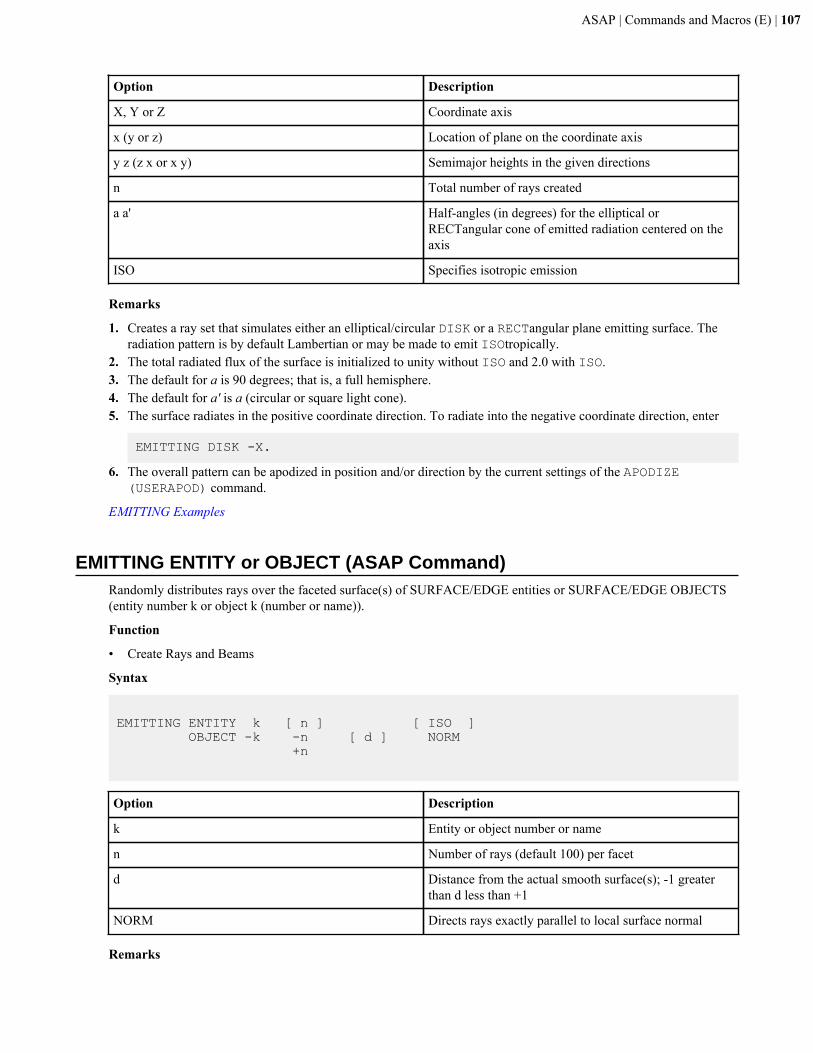
ASAP | Commands and Macros (E) | 107
Option Description
X, Y or Z Coordinate axis
x (y or z) Location of plane on the coordinate axis
y z (z x or x y) Semimajor heights in the given directions
n Total number of rays created
a a' Half-angles (in degrees) for the elliptical orRECTangular cone of emitted radiation centered on theaxis
ISO Specifies isotropic emission
Remarks
1. Creates a ray set that simulates either an elliptical/circular DISK or a RECTangular plane emitting surface. Theradiation pattern is by default Lambertian or may be made to emit ISOtropically.
2. The total radiated flux of the surface is initialized to unity without ISO and 2.0 with ISO.3. The default for a is 90 degrees; that is, a full hemisphere.4. The default for a' is a (circular or square light cone).5. The surface radiates in the positive coordinate direction. To radiate into the negative coordinate direction, enter
EMITTING DISK -X.
6. The overall pattern can be apodized in position and/or direction by the current settings of the APODIZE(USERAPOD) command.
EMITTING Examples
EMITTING ENTITY or OBJECT (ASAP Command)Randomly distributes rays over the faceted surface(s) of SURFACE/EDGE entities or SURFACE/EDGE OBJECTS(entity number k or object k (number or name)).
Function
• Create Rays and Beams
Syntax
EMITTING ENTITY k [ n ] [ ISO ] OBJECT -k -n [ d ] NORM +n
Option Description
k Entity or object number or name
n Number of rays (default 100) per facet
d Distance from the actual smooth surface(s); -1 greaterthan d less than +1
NORM Directs rays exactly parallel to local surface normal
Remarks
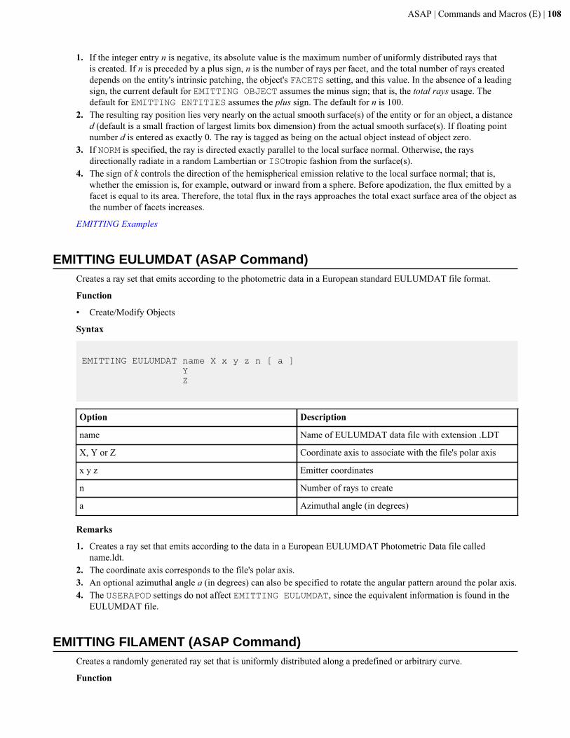
ASAP | Commands and Macros (E) | 108
1. If the integer entry n is negative, its absolute value is the maximum number of uniformly distributed rays thatis created. If n is preceded by a plus sign, n is the number of rays per facet, and the total number of rays createddepends on the entity's intrinsic patching, the object's FACETS setting, and this value. In the absence of a leadingsign, the current default for EMITTING OBJECT assumes the minus sign; that is, the total rays usage. Thedefault for EMITTING ENTITIES assumes the plus sign. The default for n is 100.
2. The resulting ray position lies very nearly on the actual smooth surface(s) of the entity or for an object, a distanced (default is a small fraction of largest limits box dimension) from the actual smooth surface(s). If floating pointnumber d is entered as exactly 0. The ray is tagged as being on the actual object instead of object zero.
3. If NORM is specified, the ray is directed exactly parallel to the local surface normal. Otherwise, the raysdirectionally radiate in a random Lambertian or ISOtropic fashion from the surface(s).
4. The sign of k controls the direction of the hemispherical emission relative to the local surface normal; that is,whether the emission is, for example, outward or inward from a sphere. Before apodization, the flux emitted by afacet is equal to its area. Therefore, the total flux in the rays approaches the total exact surface area of the object asthe number of facets increases.
EMITTING Examples
EMITTING EULUMDAT (ASAP Command)Creates a ray set that emits according to the photometric data in a European standard EULUMDAT file format.
Function
• Create/Modify Objects
Syntax
EMITTING EULUMDAT name X x y z n [ a ] Y Z
Option Description
name Name of EULUMDAT data file with extension .LDT
X, Y or Z Coordinate axis to associate with the file's polar axis
x y z Emitter coordinates
n Number of rays to create
a Azimuthal angle (in degrees)
Remarks
1. Creates a ray set that emits according to the data in a European EULUMDAT Photometric Data file calledname.ldt.
2. The coordinate axis corresponds to the file's polar axis.3. An optional azimuthal angle a (in degrees) can also be specified to rotate the angular pattern around the polar axis.4. The USERAPOD settings do not affect EMITTING EULUMDAT, since the equivalent information is found in the
EULUMDAT file.
EMITTING FILAMENT (ASAP Command)Creates a randomly generated ray set that is uniformly distributed along a predefined or arbitrary curve.
Function
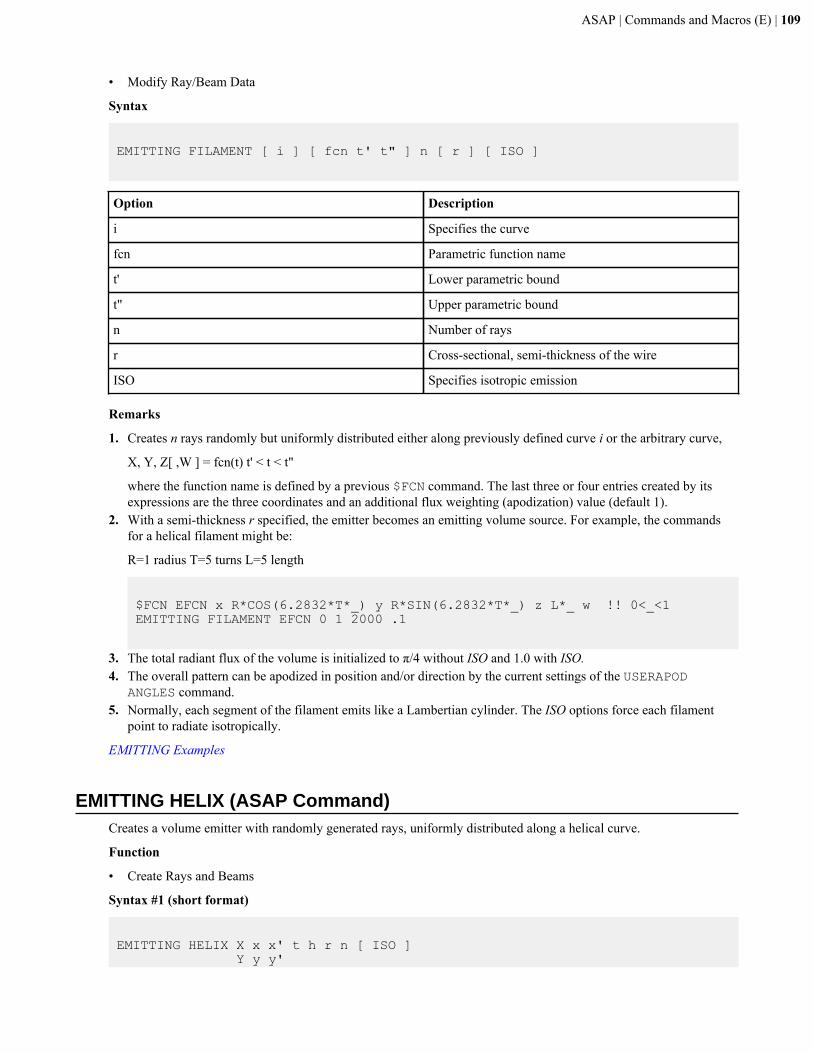
ASAP | Commands and Macros (E) | 109
• Modify Ray/Beam Data
Syntax
EMITTING FILAMENT [ i ] [ fcn t' t" ] n [ r ] [ ISO ]
Option Description
i Specifies the curve
fcn Parametric function name
t' Lower parametric bound
t" Upper parametric bound
n Number of rays
r Cross-sectional, semi-thickness of the wire
ISO Specifies isotropic emission
Remarks
1. Creates n rays randomly but uniformly distributed either along previously defined curve i or the arbitrary curve,
X, Y, Z[ ,W ] = fcn(t) t' < t < t"
where the function name is defined by a previous $FCN command. The last three or four entries created by itsexpressions are the three coordinates and an additional flux weighting (apodization) value (default 1).
2. With a semi-thickness r specified, the emitter becomes an emitting volume source. For example, the commandsfor a helical filament might be:
R=1 radius T=5 turns L=5 length
$FCN EFCN x R*COS(6.2832*T*_) y R*SIN(6.2832*T*_) z L*_ w !! 0<_<1EMITTING FILAMENT EFCN 0 1 2000 .1
3. The total radiant flux of the volume is initialized to π/4 without ISO and 1.0 with ISO.4. The overall pattern can be apodized in position and/or direction by the current settings of the USERAPOD
ANGLES command.5. Normally, each segment of the filament emits like a Lambertian cylinder. The ISO options force each filament
point to radiate isotropically.
EMITTING Examples
EMITTING HELIX (ASAP Command)Creates a volume emitter with randomly generated rays, uniformly distributed along a helical curve.
Function
• Create Rays and Beams
Syntax #1 (short format)
EMITTING HELIX X x x' t h r n [ ISO ] Y y y'
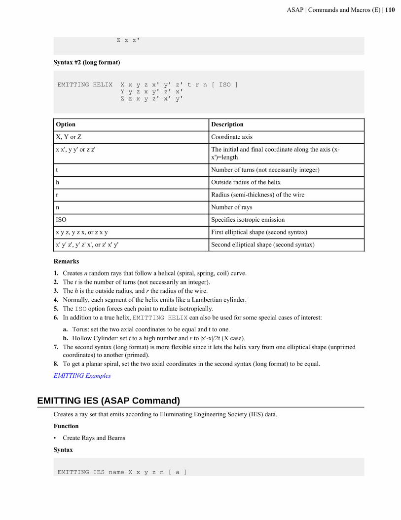
ASAP | Commands and Macros (E) | 110
Z z z'
Syntax #2 (long format)
EMITTING HELIX X x y z x' y' z' t r n [ ISO ] Y y z x y' z' x' Z z x y z' x' y'
Option Description
X, Y or Z Coordinate axis
x x', y y' or z z' The initial and final coordinate along the axis (x-x')=length
t Number of turns (not necessarily integer)
h Outside radius of the helix
r Radius (semi-thickness) of the wire
n Number of rays
ISO Specifies isotropic emission
x y z, y z x, or z x y First elliptical shape (second syntax)
x' y' z', y' z' x', or z' x' y' Second elliptical shape (second syntax)
Remarks
1. Creates n random rays that follow a helical (spiral, spring, coil) curve.2. The t is the number of turns (not necessarily an integer).3. The h is the outside radius, and r the radius of the wire.4. Normally, each segment of the helix emits like a Lambertian cylinder.5. The ISO option forces each point to radiate isotropically.6. In addition to a true helix, EMITTING HELIX can also be used for some special cases of interest:
a. Torus: set the two axial coordinates to be equal and t to one.b. Hollow Cylinder: set t to a high number and r to |x'-x|/2t (X case).
7. The second syntax (long format) is more flexible since it lets the helix vary from one elliptical shape (unprimedcoordinates) to another (primed).
8. To get a planar spiral, set the two axial coordinates in the second syntax (long format) to be equal.
EMITTING Examples
EMITTING IES (ASAP Command)Creates a ray set that emits according to Illuminating Engineering Society (IES) data.
Function
• Create Rays and Beams
Syntax
EMITTING IES name X x y z n [ a ]
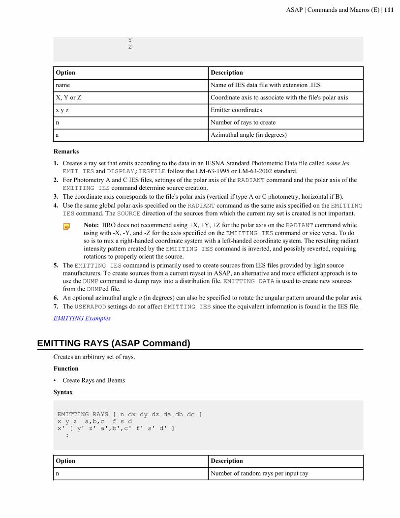
ASAP | Commands and Macros (E) | 111
Y Z
Option Description
name Name of IES data file with extension .IES
X, Y or Z Coordinate axis to associate with the file's polar axis
x y z Emitter coordinates
n Number of rays to create
a Azimuthal angle (in degrees)
Remarks
1. Creates a ray set that emits according to the data in an IESNA Standard Photometric Data file called name.ies.EMIT IES and DISPLAY;IESFILE follow the LM-63-1995 or LM-63-2002 standard.
2. For Photometry A and C IES files, settings of the polar axis of the RADIANT command and the polar axis of theEMITTING IES command determine source creation.
3. The coordinate axis corresponds to the file's polar axis (vertical if type A or C photometry, horizontal if B).4. Use the same global polar axis specified on the RADIANT command as the same axis specified on the EMITTING
IES command. The SOURCE direction of the sources from which the current ray set is created is not important.
Note: BRO does not recommend using +X, +Y, +Z for the polar axis on the RADIANT command whileusing with -X, -Y, and -Z for the axis specified on the EMIITING IES command or vice versa. To doso is to mix a right-handed coordinate system with a left-handed coordinate system. The resulting radiantintensity pattern created by the EMIITING IES command is inverted, and possibly reverted, requiringrotations to properly orient the source.
5. The EMITTING IES command is primarily used to create sources from IES files provided by light sourcemanufacturers. To create sources from a current rayset in ASAP, an alternative and more efficient approach is touse the DUMP command to dump rays into a distribution file. EMITTING DATA is used to create new sourcesfrom the DUMPed file.
6. An optional azimuthal angle a (in degrees) can also be specified to rotate the angular pattern around the polar axis.7. The USERAPOD settings do not affect EMITTING IES since the equivalent information is found in the IES file.
EMITTING Examples
EMITTING RAYS (ASAP Command)Creates an arbitrary set of rays.
Function
• Create Rays and Beams
Syntax
EMITTING RAYS [ n dx dy dz da db dc ]x y z a,b,c f s dx' [ y' z' a',b',c' f' s' d' ] :
Option Description
n Number of random rays per input ray
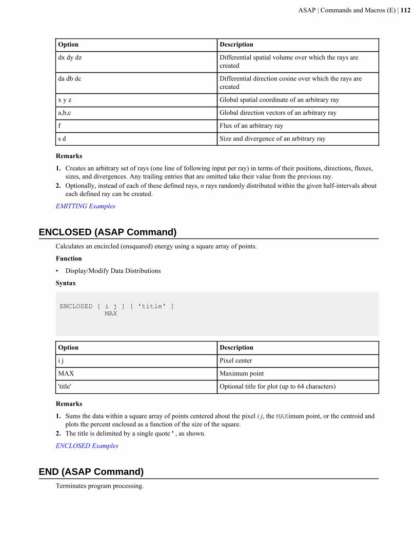
ASAP | Commands and Macros (E) | 112
Option Description
dx dy dz Differential spatial volume over which the rays arecreated
da db dc Differential direction cosine over which the rays arecreated
x y z Global spatial coordinate of an arbitrary ray
a,b,c Global direction vectors of an arbitrary ray
f Flux of an arbitrary ray
s d Size and divergence of an arbitrary ray
Remarks
1. Creates an arbitrary set of rays (one line of following input per ray) in terms of their positions, directions, fluxes,sizes, and divergences. Any trailing entries that are omitted take their value from the previous ray.
2. Optionally, instead of each of these defined rays, n rays randomly distributed within the given half-intervals abouteach defined ray can be created.
EMITTING Examples
ENCLOSED (ASAP Command)Calculates an encircled (ensquared) energy using a square array of points.
Function
• Display/Modify Data Distributions
Syntax
ENCLOSED [ i j ] [ 'title' ] MAX
Option Description
i j Pixel center
MAX Maximum point
'title' Optional title for plot (up to 64 characters)
Remarks
1. Sums the data within a square array of points centered about the pixel i j, the MAXimum point, or the centroid andplots the percent enclosed as a function of the size of the square.
2. The title is delimited by a single quote ' , as shown.
ENCLOSED Examples
END (ASAP Command)Terminates program processing.
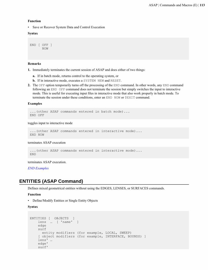
ASAP | Commands and Macros (E) | 113
Function
• Save or Recover System Data and Control Execution
Syntax
END [ OFF ] NOW
Remarks
1. Immediately terminates the current session of ASAP and does either of two things:
a. If in batch mode, returns control to the operating system, orb. If in interactive mode, executes a SYSTEM NEW and RESET.
2. The OFF option temporarily turns off the processing of the END command. In other words, any END commandfollowing an END OFF command does not terminate the session but simply switches the input to interactivemode. This is useful for executing input files in interactive mode that also work properly in batch mode. Toterminate the session under these conditions, enter an END NOW or $EXIT command.
Examples
...(other ASAP commands entered in batch mode)...END OFF
toggles input to interactive mode
...(other ASAP commands entered in interactive mode)...END NOW
terminates ASAP execution
...(other ASAP commands entered in interactive mode)...END
terminates ASAP execution.
END Examples
ENTITIES (ASAP Command)Defines mixed geometrical entities without using the EDGES, LENSES, or SURFACES commands.
Function
• Define/Modify Entities or Single Entity Objects
Syntax
ENTITIES [ OBJECTS ] lens … [ 'name' ] edge surf entity modifiers (for example, LOCAL, SWEEP) [ object modifiers (for example, INTERFACE, BOUNDS) ] lens' … edge' surf'
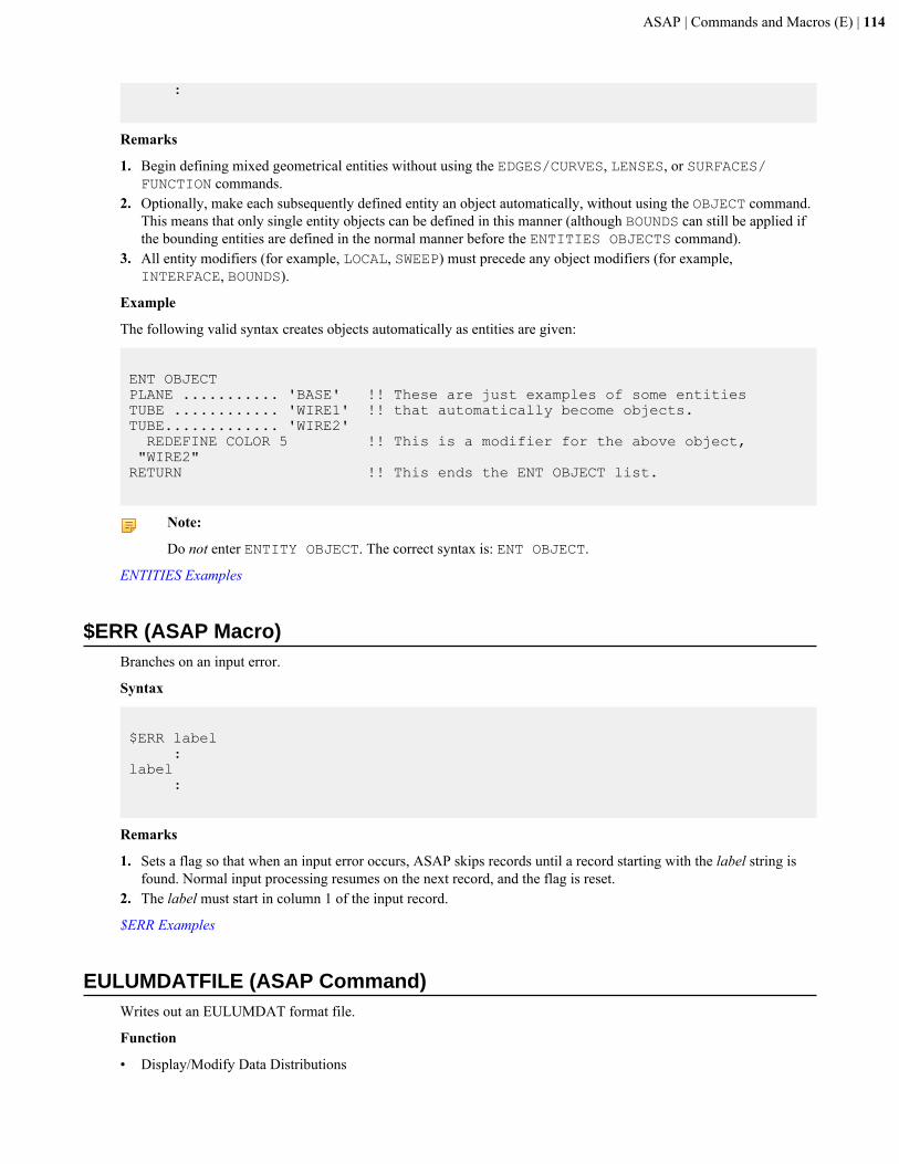
ASAP | Commands and Macros (E) | 114
:
Remarks
1. Begin defining mixed geometrical entities without using the EDGES/CURVES, LENSES, or SURFACES/FUNCTION commands.
2. Optionally, make each subsequently defined entity an object automatically, without using the OBJECT command.This means that only single entity objects can be defined in this manner (although BOUNDS can still be applied ifthe bounding entities are defined in the normal manner before the ENTITIES OBJECTS command).
3. All entity modifiers (for example, LOCAL, SWEEP) must precede any object modifiers (for example,INTERFACE, BOUNDS).
Example
The following valid syntax creates objects automatically as entities are given:
ENT OBJECT PLANE ........... 'BASE' !! These are just examples of some entitiesTUBE ............ 'WIRE1' !! that automatically become objects.TUBE............. 'WIRE2' REDEFINE COLOR 5 !! This is a modifier for the above object, "WIRE2"RETURN !! This ends the ENT OBJECT list.
Note:
Do not enter ENTITY OBJECT. The correct syntax is: ENT OBJECT.
ENTITIES Examples
$ERR (ASAP Macro)Branches on an input error.
Syntax
$ERR label :label :
Remarks
1. Sets a flag so that when an input error occurs, ASAP skips records until a record starting with the label string isfound. Normal input processing resumes on the next record, and the flag is reset.
2. The label must start in column 1 of the input record.
$ERR Examples
EULUMDATFILE (ASAP Command)Writes out an EULUMDAT format file.
Function
• Display/Modify Data Distributions
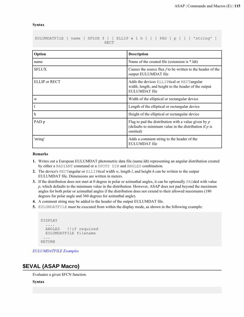
ASAP | Commands and Macros (E) | 115
Syntax
EULUMDATFILE [ name [ SFLUX f ] [ ELLIP w l h ] ] [ PAD [ p ] ] [ 'string' ] RECT
Option Description
name Name of the created file (extension is *.ldt)
SFLUX Causes the source flux f to be written to the header of theoutput EULUMDAT file
ELLIP or RECT Adds the devices ELLIPtical or RECTangularwidth, length, and height to the header of the outputEULUMDAT file
w Width of the elliptical or rectangular device
l Length of the elliptical or rectangular device
h Height of the elliptical or rectangular device
PAD p Flag to pad the distribution with a value given by p(defaults to minimum value in the distribution if p isomitted)
'string' Adds a comment string to the header of theEULUMDAT file
Remarks
1. Writes out a European EULUMDAT photometric data file (name.ldt) representing an angular distribution createdby either a RADIANT command or a SPOTS DIR and ANGLES combination.
2. The device's RECTangular or ELLIPtical width w, length l, and height h can be written to the outputEULUMDAT file. Dimensions are written in meters.
3. If the distribution does not start at 0 degree in polar or azimuthal angles, it can be optionally PADded with valuep, which defaults to the minimum value in the distribution. However, ASAP does not pad beyond the maximumangles for both polar or azimuthal angles if the distribution does not extend to their allowed maximums (180degrees for polar angle and 360 degrees for azimuthal angle).
4. A comment string may be added to the header of the output EULUMDAT file.5. EULUMDATFILE must be executed from within the display mode, as shown in the following example:
DISPLAY .... ANGLES !!if required EULUMDATFILE filename ...RETURN
EULUMDATFILE Examples
$EVAL (ASAP Macro)Evaluates a given $FCN function.
Syntax
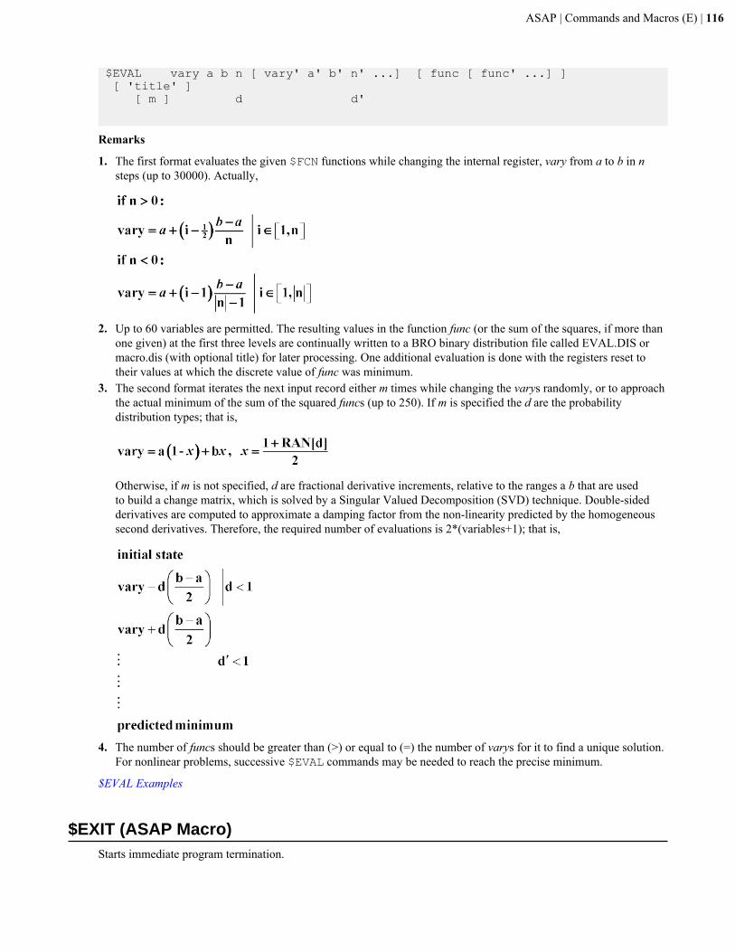
ASAP | Commands and Macros (E) | 116
$EVAL vary a b n [ vary' a' b' n' ...] [ func [ func' ...] ] [ 'title' ] [ m ] d d'
Remarks
1. The first format evaluates the given $FCN functions while changing the internal register, vary from a to b in nsteps (up to 30000). Actually,
2. Up to 60 variables are permitted. The resulting values in the function func (or the sum of the squares, if more thanone given) at the first three levels are continually written to a BRO binary distribution file called EVAL.DIS ormacro.dis (with optional title) for later processing. One additional evaluation is done with the registers reset totheir values at which the discrete value of func was minimum.
3. The second format iterates the next input record either m times while changing the varys randomly, or to approachthe actual minimum of the sum of the squared funcs (up to 250). If m is specified the d are the probabilitydistribution types; that is,
Otherwise, if m is not specified, d are fractional derivative increments, relative to the ranges a b that are usedto build a change matrix, which is solved by a Singular Valued Decomposition (SVD) technique. Double-sidedderivatives are computed to approximate a damping factor from the non-linearity predicted by the homogeneoussecond derivatives. Therefore, the required number of evaluations is 2*(variables+1); that is,
4. The number of funcs should be greater than (>) or equal to (=) the number of varys for it to find a unique solution.For nonlinear problems, successive $EVAL commands may be needed to reach the precise minimum.
$EVAL Examples
$EXIT (ASAP Macro)Starts immediate program termination.
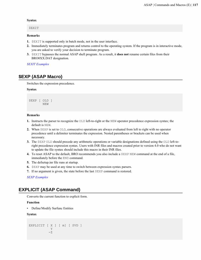
ASAP | Commands and Macros (E) | 117
Syntax
$EXIT
Remarks
1. $EXIT is supported only in batch mode, not in the user interface.2. Immediately terminates program and returns control to the operating system. If the program is in interactive mode,
you are asked to verify your decision to terminate program.3. $EXIT bypasses the normal ASAP shell program. As a result, it does not rename certain files from their
BRO0XX.DAT designation.
$EXIT Examples
$EXP (ASAP Macro)Switches the expression precedence.
Syntax
$EXP [ OLD ] NEW
Remarks
1. Instructs the parser to recognize the OLD left-to-right or the NEW operator precedence expression syntax; thedefault is NEW.
2. When $EXP is set to OLD, consecutive operations are always evaluated from left to right with no operatorprecedence until a delimiter terminates the expression. Nested parentheses or brackets can be used whennecessary.
3. The $EXP OLD should precede any arithmetic operations or variable designations defined using the OLD left-to-right precedence expression syntax. Users with INR files and macros created prior to version 4.0 who do not wantto update the file syntax should include this macro in their INR files.
4. To reset ASAP to the default, BRO recommends you also include a $EXP NEW command at the end of a file,immediately before the END command.
5. The defsetup.inr file runs at startup.6. $EXP may be used at any time to switch between expression syntax parsers.7. If no argument is given, the state before the last $EXP command is restored.
$EXP Examples
EXPLICIT (ASAP Command)Converts the current function to explicit form.
Function
• Define/Modify Surfunc Entities
Syntax
EXPLICIT [ X ] [ m] [ SVD ] Y -Z
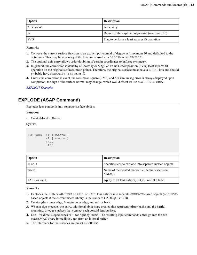
ASAP | Commands and Macros (E) | 118
Option Description
X, Y, or -Z Axis entry
m Degree of the explicit polynomial (maximum 20)
SVD Flag to perform a least squares fit operation
Remarks
1. Converts the current surface function to an explicit polynomial of degree m (maximum 20 and defaulted to theoptimum). This may be necessary if the function is used as a DEFORM on an OBJECT.
2. The optional axis entry allows order doubling of certain coordinates to enforce symmetry.3. In general, the conversion is done by a Cholesky or Singular Value Decomposition (SVD) least squares fit
operation on the original surface's mesh points. Therefore, the original surface must have a LOCAL box and shouldprobably have PARAMETERIZE set to -Z.
4. Unless the conversion is exact, the root-mean square (RMS) and MAXimum sag error is always displayed uponcompletion, the sign of the surface normal may change, which would affect its use as a BOUNDS entity.
EXPLICIT Examples
EXPLODE (ASAP Command)Explodes lens conicoids into separate surface objects.
Function
• Create/Modify Objects
Syntax
EXPLODE +l [ macro ] -l [ macro ] +ALL -ALL
Option Description
+l or -1 Specifies lens to explode into separate surface objects
macro Name of the created macro file (default extension*.MAC)
+ALL or -ALL Apply to all lens entities, not just one at a time
Remarks
1. Explodes the + lth or -lth LENS or +ALL or -ALL lens entities into separate SURFACE-based objects (or CURVE-based objects if the current macro library is the standard CADEQUIV.LIB).
2. Creates glass inner edge, Mangin outer edge, and mirror back.3. When a sign precedes the entry, additional objects are created that represent mirror backs and the baffle,
mounting, or edge surfaces that connect each coaxial lens surface.4. Use - for direct sloped cones or + for right cylinders. The resulting input commands either go into the file
macro.MAC or are immediately run from an internal buffer.5. The interfaces for the surfaces are preset as follows:
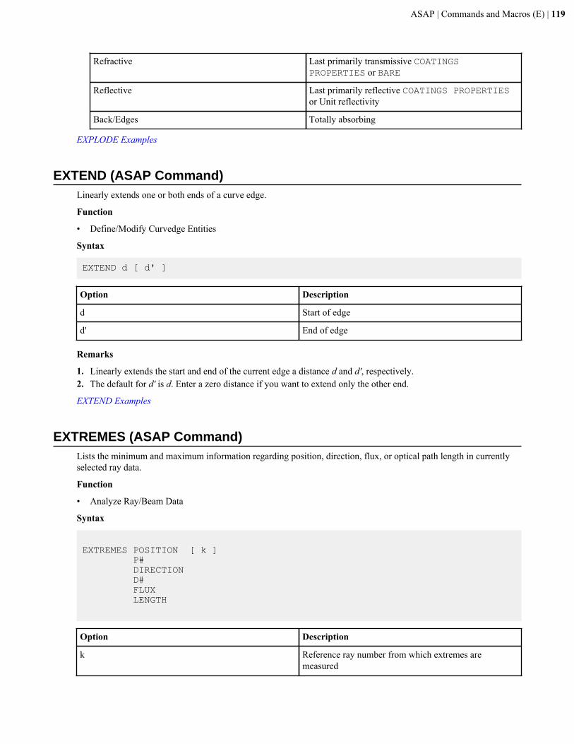
ASAP | Commands and Macros (E) | 119
Refractive Last primarily transmissive COATINGSPROPERTIES or BARE
Reflective Last primarily reflective COATINGS PROPERTIESor Unit reflectivity
Back/Edges Totally absorbing
EXPLODE Examples
EXTEND (ASAP Command)Linearly extends one or both ends of a curve edge.
Function
• Define/Modify Curvedge Entities
Syntax
EXTEND d [ d' ]
Option Description
d Start of edge
d' End of edge
Remarks
1. Linearly extends the start and end of the current edge a distance d and d', respectively.2. The default for d' is d. Enter a zero distance if you want to extend only the other end.
EXTEND Examples
EXTREMES (ASAP Command)Lists the minimum and maximum information regarding position, direction, flux, or optical path length in currentlyselected ray data.
Function
• Analyze Ray/Beam Data
Syntax
EXTREMES POSITION [ k ] P# DIRECTION D# FLUX LENGTH
Option Description
k Reference ray number from which extremes aremeasured
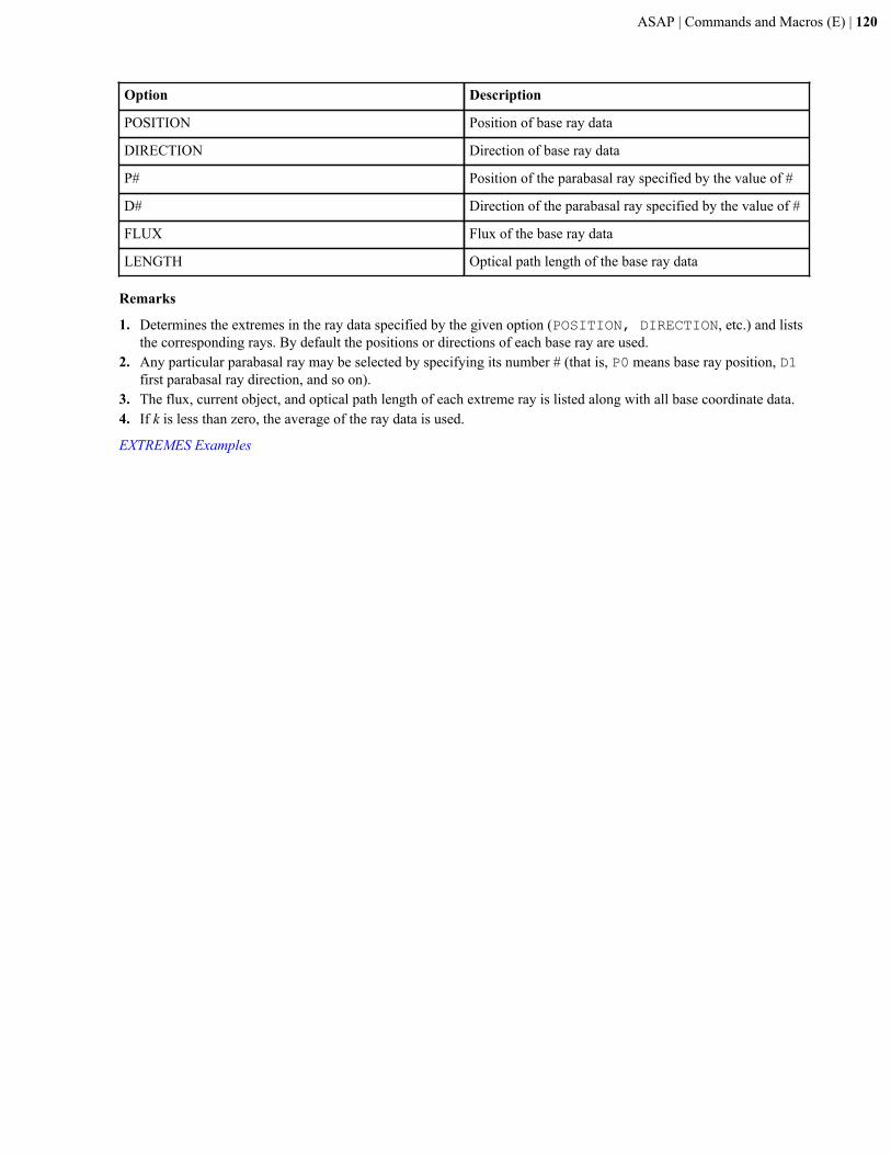
ASAP | Commands and Macros (E) | 120
Option Description
POSITION Position of base ray data
DIRECTION Direction of base ray data
P# Position of the parabasal ray specified by the value of #
D# Direction of the parabasal ray specified by the value of #
FLUX Flux of the base ray data
LENGTH Optical path length of the base ray data
Remarks
1. Determines the extremes in the ray data specified by the given option (POSITION, DIRECTION, etc.) and liststhe corresponding rays. By default the positions or directions of each base ray are used.
2. Any particular parabasal ray may be selected by specifying its number # (that is, P0 means base ray position, D1first parabasal ray direction, and so on).
3. The flux, current object, and optical path length of each extreme ray is listed along with all base coordinate data.4. If k is less than zero, the average of the ray data is used.
EXTREMES Examples
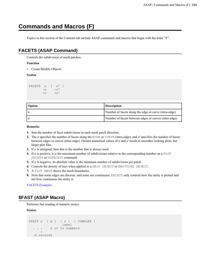
ASAP | Commands and Macros (F) | 121
Commands and Macros (F)
Topics in this section of the Contents tab include ASAP commands and macros that begin with the letter “F”.
FACETS (ASAP Command)Controls the subdivision of mesh patches.
Function
• Create/Modify Objects
Syntax
FACETS n [ n' ] -n -n' +n +n'
Option Description
n Number of facets along the edge or curve (intra-edge)
n' Number of facets between edges or curves (inter-edge)
Remarks
1. Sets the number of facet subdivisions in each mesh patch direction.2. The n specifies the number of facets along the EDGE or CURVE (intra-edge), and n' specifies the number of facets
between edges or curves (inter-edge). Greater numerical values of n and n' result in smoother looking plots, butlarger plot files.
3. If n is unsigned, then this is the number that is always used.4. If n is positive, it is the maximum number of subdivisions relative to the corresponding number on a PLOT
FACETS or VUFACETS command.5. If n is negative, its absolute value is the minimum number of subdivisions per patch.6. Controls the density of rays when applied to a GRID OBJECT or EMITTING OBJECT.7. A PLOT MESH shows the mesh boundaries.8. Note that some edges are discrete, and some are continuous; FACETS only controls how the entity is plotted and
not how continuous the entity is.
FACETS Examples
$FAST (ASAP Macro)Performs fast reading of numeric arrays.
Syntax
$FAST n [ m ] [ s ] [ COMPLEX ] label . . . n or 2n numbers : m records
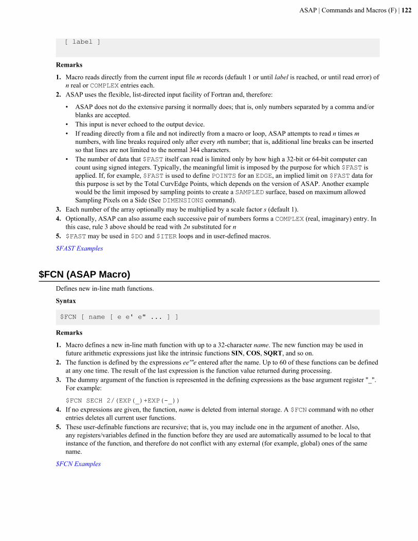
ASAP | Commands and Macros (F) | 122
[ label ]
Remarks
1. Macro reads directly from the current input file m records (default 1 or until label is reached, or until read error) ofn real or COMPLEX entries each.
2. ASAP uses the flexible, list-directed input facility of Fortran and, therefore:
• ASAP does not do the extensive parsing it normally does; that is, only numbers separated by a comma and/orblanks are accepted.
• This input is never echoed to the output device.• If reading directly from a file and not indirectly from a macro or loop, ASAP attempts to read n times m
numbers, with line breaks required only after every nth number; that is, additional line breaks can be insertedso that lines are not limited to the normal 344 characters.
• The number of data that $FAST itself can read is limited only by how high a 32-bit or 64-bit computer cancount using signed integers. Typically, the meaningful limit is imposed by the purpose for which $FAST isapplied. If, for example, $FAST is used to define POINTS for an EDGE, an implied limit on $FAST data forthis purpose is set by the Total CurvEdge Points, which depends on the version of ASAP. Another examplewould be the limit imposed by sampling points to create a SAMPLED surface, based on maximum allowedSampling Pixels on a Side (See DIMENSIONS command).
3. Each number of the array optionally may be multiplied by a scale factor s (default 1).4. Optionally, ASAP can also assume each successive pair of numbers forms a COMPLEX (real, imaginary) entry. In
this case, rule 3 above should be read with 2n substituted for n5. $FAST may be used in $DO and $ITER loops and in user-defined macros.
$FAST Examples
$FCN (ASAP Macro)Defines new in-line math functions.
Syntax
$FCN [ name [ e e' e" ... ] ]
Remarks
1. Macro defines a new in-line math function with up to a 32-character name. The new function may be used infuture arithmetic expressions just like the intrinsic functions SIN, COS, SQRT, and so on.
2. The function is defined by the expressions ee'"e entered after the name. Up to 60 of these functions can be definedat any one time. The result of the last expression is the function value returned during processing.
3. The dummy argument of the function is represented in the defining expressions as the base argument register "_".For example:
$FCN SECH 2/(EXP(_)+EXP(-_))4. If no expressions are given, the function, name is deleted from internal storage. A $FCN command with no other
entries deletes all current user functions.5. These user-definable functions are recursive; that is, you may include one in the argument of another. Also,
any registers/variables defined in the function before they are used are automatically assumed to be local to thatinstance of the function, and therefore do not conflict with any external (for example, global) ones of the samename.
$FCN Examples
ASAP | Commands and Macros (F) | 123
$FF (ASAP Macro)Inserts a form feed into the output stream.
Syntax
$FF [ text ]&FF k
Remarks
1. If $ prefix is used, a page advances or form feed is sent to the current output unit. Any text present on thiscommand (up to 62 characters) is also printed at the top of the page along with the current date and time.
2. The integer entry form outputs only a form feed to logical unit k instead.3. If the &FF syntax is used, only the text (up to 80 characters) that is preceded and followed by single blank lines is
written.
$FF Examples
FFAD (ASAP Command)Formats currently selected ray data and plots full-field aberration displays (FFAD).
Function
• Analyze Ray/Beam Data
Syntax
FFAD [ SPOTS [ s ] ] [ REFERENCE w [k] ] [ LIST ]
Option Description
SPOTS Plots spot diagram at each field point
s Spot diagram scale factor
REFERENCE w k Smallest spot identifier
LIST Lists the flux, centroids, and RMS sizes of each source
Remarks
1. Produces a real Full Field Aberration Display, which is a plot of the 3D best-focused RMS spot ellipses for eachfield position entered on the SOURCE command. The ellipses are scaled up so that the largest one just touches thespot from an adjacent field position. These plots are useful for identifying aberration nodes on the image surfacesof non-centered or perturbed systems.
2. FFAD prints the statistics of the spots, including the best-fit planar and curved surface parameters.3. The corresponding unfocused ray SPOTS can also be plotted. The s (default=0.3) is an additional scale factor used
to make room for the spot patterns since they are always larger than the RMS ellipses.4. The REFERENCE option specifies the width w (in system units) of a square that is drawn around the smallest (or
kth) spot.5. FFAD also prints out the statistics of the spots including the best-fit planar and curved surface parameters.6. The flux, centroids, and RMS sizes of each source can also be LISTed.
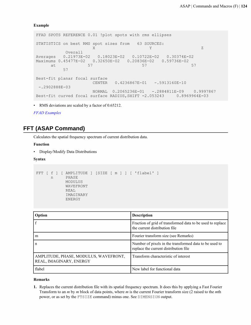
ASAP | Commands and Macros (F) | 124
Example
FFAD SPOTS REFERENCE 0.01 !plot spots with rms ellipses
STATISTICS on best RMS spot sizes from 63 SOURCES: X Y Z OverallAverages 0.21973E-02 0.18023E-02 0.10722E-02 0.30374E-02Maximums 0.45477E-02 0.32650E-02 0.20836E-02 0.59736E-02 at 57 57 57 57
Best-fit planar focal surface CENTER 0.4236867E-01 -.5913160E-10 -.2902888E-03 NORMAL 0.2065236E-01 -.2884811E-09 0.9997867Best-fit curved focal surface RADIUS,SHIFT -2.053243 0.8969964E-03
• RMS deviations are scaled by a factor of 0.65212.
FFAD Examples
FFT (ASAP Command)Calculates the spatial frequency spectrum of current distribution data.
Function
• Display/Modify Data Distributions
Syntax
FFT [ f ] [ AMPLITUDE ] [SIZE [ m ] ] [ 'flabel' ] n PHASE MODULUS WAVEFRONT REAL IMAGINARY ENERGY
Option Description
f Fraction of grid of transformed data to be used to replacethe current distribution file
m Fourier transform size (see Remarks)
n Number of pixels in the transformed data to be used toreplace the current distribution file
AMPLITUDE, PHASE, MODULUS, WAVEFRONT,REAL, IMAGINARY, ENERGY
Transform characteristic of interest
flabel New label for functional data
Remarks
1. Replaces the current distribution file with its spatial frequency spectrum. It does this by applying a Fast FourierTransform to an m by m block of data points, where m is the current Fourier transform size (2 raised to the mthpower, or as set by the FTSIZE command) minus one. See DIMENSION output.

ASAP | Commands and Macros (F) | 125
2. If the original data area is smaller than m-by-m, the data is centered and any excess is zero filled.3. If the original data area is larger, you must make sure that most of the energy lies in the first m-by-m block. ASAP
then takes the selected part (default MODULUS) of the center n-by-n or f*m-by-b*m area of the FFT as the currentdata set.
4. If f is an integer n greater than one, it is the actual number of pixels to use. ASAP calculates the default for n tomaintain the original data size.
5. If f or n, are a negative number, the inverse FFT operation is performed.6. Applying the FFT command to the diffraction image of a point object generated by a SPREAD or OPDMAP
command produces the classical MTF (Modulation Transfer Function) of the system.7. The spacing S' between sample points after the FFT is related to the original spacing S by:
where the maximum pixel value determines the constant in the above expression.
Use the flabel option to relabel the functional data.8. If the Fourier transformed field U(p,q) is written in the form:
where A(p,q) is the real part and B(p,q) is the imaginary part of the field, then the components of the complexfield that can be displayed include:
Option Operation Physical Significance
AMPLITUDE sign(real( U )) | U | signed modulus of field
PHASE arctan( B / A ) phase in radians
MODULUS | U | modulus of the field
WAVEFRONT arctan( B / A ) / 2 p wavefront in waves
REAL real( U ) or A real part of field
IMAGINARY imaginary( U ) or B imaginary part of field
ENERGY U U* modulus squared of field (energydensity)
9. The phase transfer function (PTF) may be obtained by extracting the phase or wavefront from the FFT operation.The wavefront is usually better choice because it attempts to remove the 2π phase steps from the wavefront.
FFT Examples
FIELD (ASAP Command)Calculates the exact complex field distribution.
Function
• Calculate Diffraction/Propagation Effects
Syntax 1
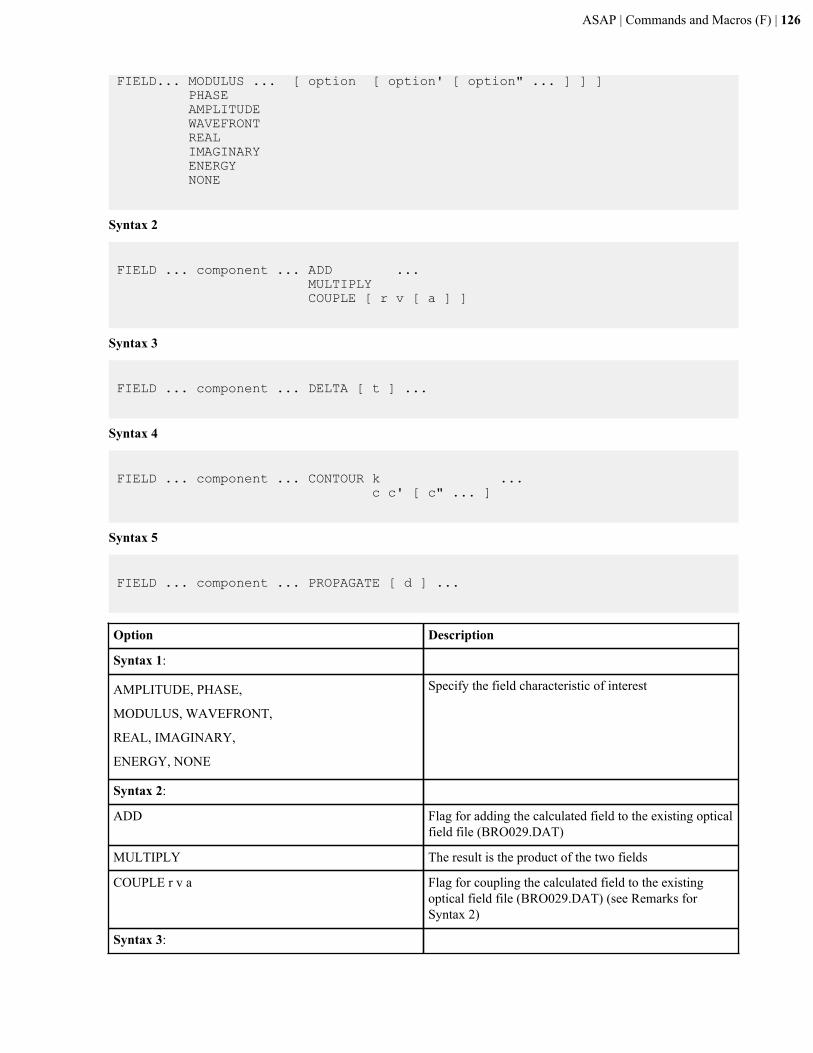
ASAP | Commands and Macros (F) | 126
FIELD... MODULUS ... [ option [ option' [ option" ... ] ] ] PHASE AMPLITUDE WAVEFRONT REAL IMAGINARY ENERGY NONE
Syntax 2
FIELD ... component ... ADD ... MULTIPLY COUPLE [ r v [ a ] ]
Syntax 3
FIELD ... component ... DELTA [ t ] ...
Syntax 4
FIELD ... component ... CONTOUR k ... c c' [ c" ... ]
Syntax 5
FIELD ... component ... PROPAGATE [ d ] ...
Option Description
Syntax 1:
AMPLITUDE, PHASE,
MODULUS, WAVEFRONT,
REAL, IMAGINARY,
ENERGY, NONE
Specify the field characteristic of interest
Syntax 2:
ADD Flag for adding the calculated field to the existing opticalfield file (BRO029.DAT)
MULTIPLY The result is the product of the two fields
COUPLE r v a Flag for coupling the calculated field to the existingoptical field file (BRO029.DAT) (see Remarks forSyntax 2)
Syntax 3:
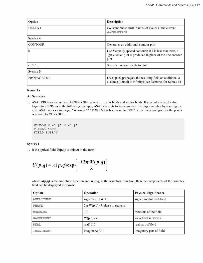
ASAP | Commands and Macros (F) | 127
Option Description
DELTA t Constant phase shift in units of cycles at the currentWAVELENGTH
Syntax 4:
CONTOUR Generates an additional contour plot
k Use k equally spaced contours; if k is less than zero, a"gray scale" plot is produced in place of the line contourplot
c c' c" ... Specific contour levels to plot
Syntax 5:
PROPAGATE d Free-space propagate the resulting field an additional ddistance (default is infinity) (see Remarks for Syntax 5)
Remarks
All Syntaxes
1. ASAP PRO can use only up to 2896X2896 pixels for scalar fields and vector fields. If you enter a pixel valuelarger than 2896, as in the following example, ASAP attempts to accommodate the larger number by resizing thegrid. ASAP issues a message: "Warning *** PIXELS has been reset to 3999", while the actual grid for the pixelsis resized to 3999X2096.
WINDOW X -2 @1 Y -2 @1PIXELS 4000FIELD ENERGY
Syntax 1
1. If the optical field U(p,q) is written in the form:
where A(p,q) is the amplitude function and W(p,q) is the wavefront function, then the components of the complexfield can be displayed as shown:
Option Operation Physical Significance
AMPLITUDE sign(real( U )) | U | signed modulus of field
PHASE 2 π W(p,q) / λ phase in radians
MODULUS | U | modulus of the field
WAVEFRONT W(p,q) / λ wavefront in waves
REAL real( U ) real part of field
IMAGINARY imaginary( U ) imaginary part of field

ASAP | Commands and Macros (F) | 128
Option Operation Physical Significance
ENERGY U U* modulus squared of field (energydensity)
NONE -- none
2. Except for NONE, writes the given component of the complex scalar (or last vector POLARIZATION) field to thestandard distribution file BRO009.DAT for later processing by DISPLAY. The original full complex scalar/vectorfield is always written to unit 29 (file BRO029.DAT).
Syntax 2
1. If the ADD option is present, the calculated complex field is added to the previously stored field in theBRO029.DAT file.
2. If the COUPLE option is present, the calculated field is coupled to the field previously stored in the file.3. Alternatively, you can directly COUPLE to the fundamental mode field of a circular fiber of core radius r,
normalized frequency v, and optional gradient index power a (for example, 2 for parabolic, absent for step index).If MULTIPLY is specified, the result is the product of the two fields. In all three cases, the two fields should becalculated under the same conditions; that is, WAVELENGTH, PIXELS, and WINDOW settings. If you attempt tocalculate under differing PIXEL conditions, ASAP issues an error and does not perform the calculation. You cancombine (with ADD, MULTIPLY, or COUPLE) any two distributions having the same PIXEL settings. Theresults are typically sensible only if the WINDOW settings and the WAVELENGTH settings also match.
Syntax 3
1. A constant phase shift t (in cycles at the current WAVELENGTH) can be added to each beam. This is equivalentto calculating the field at a time other than t=0. If this DELTA option is present and a vector field is beingcalculated (that is, FRESNEL BOTH is set), ASAP produces a plot of polarization ellipses, or if t is given, arrowsrepresenting the relative magnitude and direction of the instantaneous electric field at each sample point.
Syntax 4
1. The CONTOUR option generates an additional contour plot with fractional contours c c' ... relative to the full rangeof the function being plotted. Alternatively, k equally spaced contours can be specified. If k is less than zero, agrey scale plot is produced instead of the line contour plot.
Syntax 5
1. At the current IMMERSE index and WAVELENGTH, free-space PROPAGATE the resulting field an additionaldistance d (default is infinity), using an approximate (ACCURACY LOW) to an exact (ACCURACY HIGH) FastFourier Transform (FFT) technique.
Note:
Regardless of the order the previous options are entered, the order in which FIELD actually performs itscalculations is as follows:
1. Read/calculate field2. ADD, MULTIPLY or COUPLE with another3. CLIP with an entity or object4. DELTA polarization plot5. PROPAGATE additional distance6. Write distribution files7. CONTOUR plot
Example
FIELD ENERGY -1
Distribution of data within: Across or Vertical: Z = -2.50000 to 2.50000 ( 5.00000 )
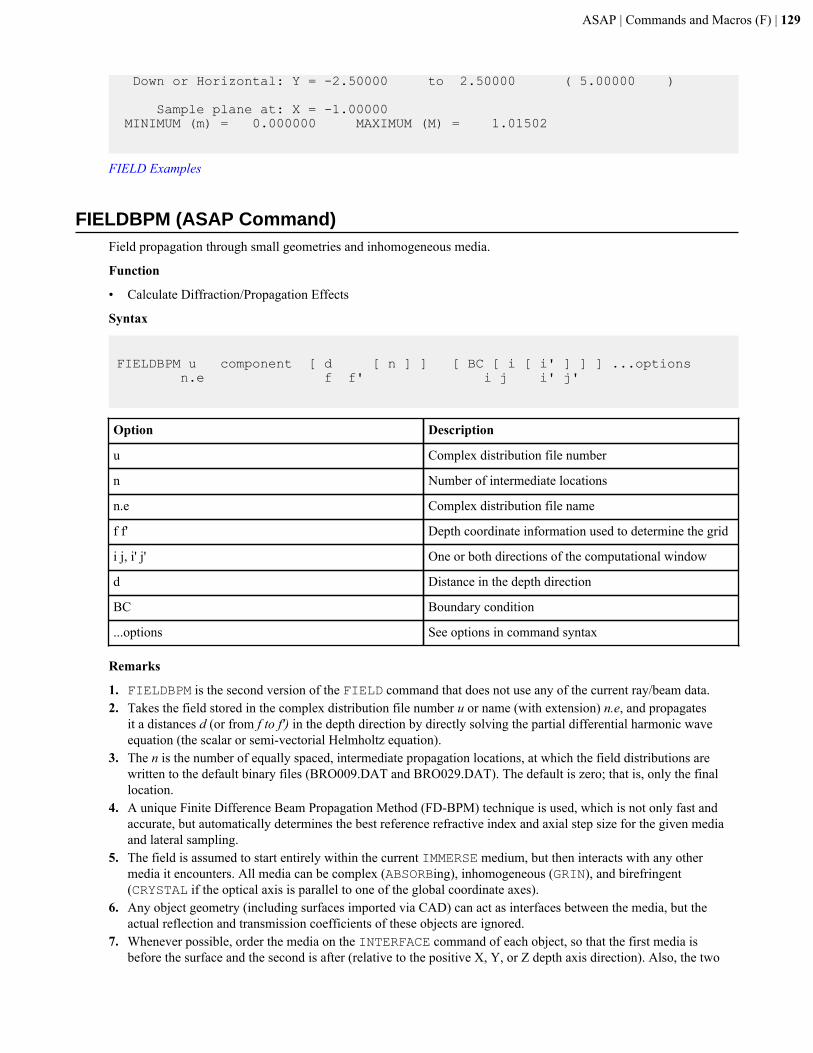
ASAP | Commands and Macros (F) | 129
Down or Horizontal: Y = -2.50000 to 2.50000 ( 5.00000 )
Sample plane at: X = -1.00000 MINIMUM (m) = 0.000000 MAXIMUM (M) = 1.01502
FIELD Examples
FIELDBPM (ASAP Command)Field propagation through small geometries and inhomogeneous media.
Function
• Calculate Diffraction/Propagation Effects
Syntax
FIELDBPM u component [ d [ n ] ] [ BC [ i [ i' ] ] ] ...options n.e f f' i j i' j'
Option Description
u Complex distribution file number
n Number of intermediate locations
n.e Complex distribution file name
f f' Depth coordinate information used to determine the grid
i j, i' j' One or both directions of the computational window
d Distance in the depth direction
BC Boundary condition
...options See options in command syntax
Remarks
1. FIELDBPM is the second version of the FIELD command that does not use any of the current ray/beam data.2. Takes the field stored in the complex distribution file number u or name (with extension) n.e, and propagates
it a distances d (or from f to f') in the depth direction by directly solving the partial differential harmonic waveequation (the scalar or semi-vectorial Helmholtz equation).
3. The n is the number of equally spaced, intermediate propagation locations, at which the field distributions arewritten to the default binary files (BRO009.DAT and BRO029.DAT). The default is zero; that is, only the finallocation.
4. A unique Finite Difference Beam Propagation Method (FD-BPM) technique is used, which is not only fast andaccurate, but automatically determines the best reference refractive index and axial step size for the given mediaand lateral sampling.
5. The field is assumed to start entirely within the current IMMERSE medium, but then interacts with any othermedia it encounters. All media can be complex (ABSORBing), inhomogeneous (GRIN), and birefringent(CRYSTAL if the optical axis is parallel to one of the global coordinate axes).
6. Any object geometry (including surfaces imported via CAD) can act as interfaces between the media, but theactual reflection and transmission coefficients of these objects are ignored.
7. Whenever possible, order the media on the INTERFACE command of each object, so that the first media isbefore the surface and the second is after (relative to the positive X, Y, or Z depth axis direction). Also, the two
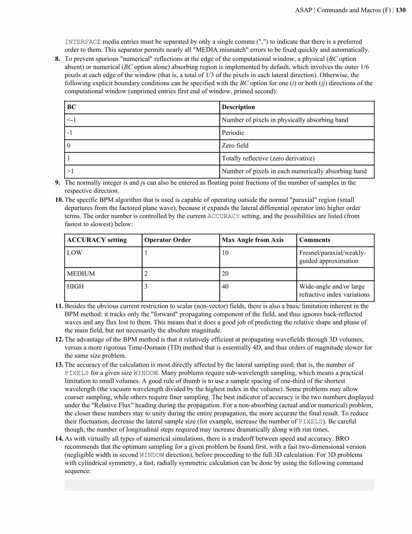
ASAP | Commands and Macros (F) | 130
INTERFACE media entries must be separated by only a single comma (",") to indicate that there is a preferredorder to them. This separator permits nearly all "MEDIA mismatch" errors to be fixed quickly and automatically.
8. To prevent spurious "numerical" reflections at the edge of the computational window, a physical (BC optionabsent) or numerical (BC option alone) absorbing region is implemented by default, which involves the outer 1/6pixels at each edge of the window (that is, a total of 1/3 of the pixels in each lateral direction). Otherwise, thefollowing explicit boundary conditions can be specified with the BC option for one (i) or both (ij) directions of thecomputational window (unprimed entries first end of window, primed second):
BC Description
<-1 Number of pixels in physically absorbing band
-1 Periodic
0 Zero field
1 Totally reflective (zero derivative)
>1 Number of pixels in each numerically absorbing band
9. The normally integer is and js can also be entered as floating point fractions of the number of samples in therespective direction.
10. The specific BPM algorithm that is used is capable of operating outside the normal "paraxial" region (smalldepartures from the factored plane wave), because it expands the lateral differential operator into higher orderterms. The order number is controlled by the current ACCURACY setting, and the possibilities are listed (fromfastest to slowest) below:
ACCURACY setting Operator Order Max Angle from Axis Comments
LOW 1 10 Fresnel/paraxial/weakly-guided approximation
MEDIUM 2 20
HIGH 3 40 Wide-angle and/or largerefractive index variations
11. Besides the obvious current restriction to scalar (non-vector) fields, there is also a basic limitation inherent in theBPM method: it tracks only the "forward" propagating component of the field, and thus ignores back-reflectedwaves and any flux lost to them. This means that it does a good job of predicting the relative shape and phase ofthe main field, but not necessarily the absolute magnitude.
12. The advantage of the BPM method is that it relatively efficient at propagating wavefields through 3D volumes,versus a more rigorous Time-Domain (TD) method that is essentially 4D, and thus orders of magnitude slower forthe same size problem.
13. The accuracy of the calculation is most directly affected by the lateral sampling used; that is, the number ofPIXELS for a given size WINDOW. Many problems require sub-wavelength sampling, which means a practicallimitation to small volumes. A good rule of thumb is to use a sample spacing of one-third of the shortestwavelength (the vacuum wavelength divided by the highest index in the volume). Some problems may allowcoarser sampling, while others require finer sampling. The best indicator of accuracy is the two numbers displayedunder the "Relative Flux" heading during the propagation. For a non-absorbing (actual and/or numerical) problem,the closer these numbers stay to unity during the entire propagation, the more accurate the final result. To reducetheir fluctuation, decrease the lateral sample size (for example, increase the number of PIXELS). Be carefulthough, the number of longitudinal steps required may increase dramatically along with run times.
14. As with virtually all types of numerical simulations, there is a tradeoff between speed and accuracy. BROrecommends that the optimum sampling for a given problem be found first, with a fast two-dimensional version(negligible width in second WINDOW direction), before proceeding to the full 3D calculation. For 3D problemswith cylindrical symmetry, a fast, radially symmetric calculation can be done by using the following commandsequence:
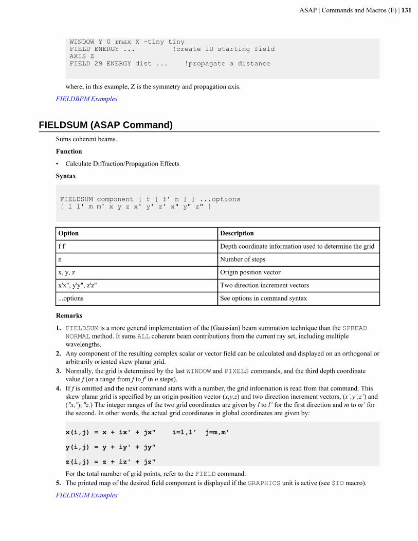
ASAP | Commands and Macros (F) | 131
WINDOW Y 0 rmax X -tiny tinyFIELD ENERGY ... !create 1D starting fieldAXIS ZFIELD 29 ENERGY dist ... !propagate a distance
where, in this example, Z is the symmetry and propagation axis.
FIELDBPM Examples
FIELDSUM (ASAP Command)Sums coherent beams.
Function
• Calculate Diffraction/Propagation Effects
Syntax
FIELDSUM component [ f [ f' n ] ] ...options[ l l' m m' x y z x' y' z' x" y" z" ]
Option Description
f f' Depth coordinate information used to determine the grid
n Number of steps
x, y, z Origin position vector
x'x", y'y", z'z" Two direction increment vectors
...options See options in command syntax
Remarks
1. FIELDSUM is a more general implementation of the (Gaussian) beam summation technique than the SPREADNORMAL method. It sums ALL coherent beam contributions from the current ray set, including multiplewavelengths.
2. Any component of the resulting complex scalar or vector field can be calculated and displayed on an orthogonal orarbitrarily oriented skew planar grid.
3. Normally, the grid is determined by the last WINDOW and PIXELS commands, and the third depth coordinatevalue f (or a range from f to f' in n steps).
4. If f is omitted and the next command starts with a number, the grid information is read from that command. Thisskew planar grid is specified by an origin position vector (x,y,z) and two direction increment vectors, (x’,y’,z’) and("x,"y,"z.) The integer ranges of the two grid coordinates are given by l to l’ for the first direction and m to m’ forthe second. In other words, the actual grid coordinates in global coordinates are given by:
x(i,j) = x + ix' + jx" i=l,l' j=m,m'
y(i,j) = y + iy' + jy"
z(i,j) = z + iz' + jz"
For the total number of grid points, refer to the FIELD command.5. The printed map of the desired field component is displayed if the GRAPHICS unit is active (see $IO macro).
FIELDSUM Examples
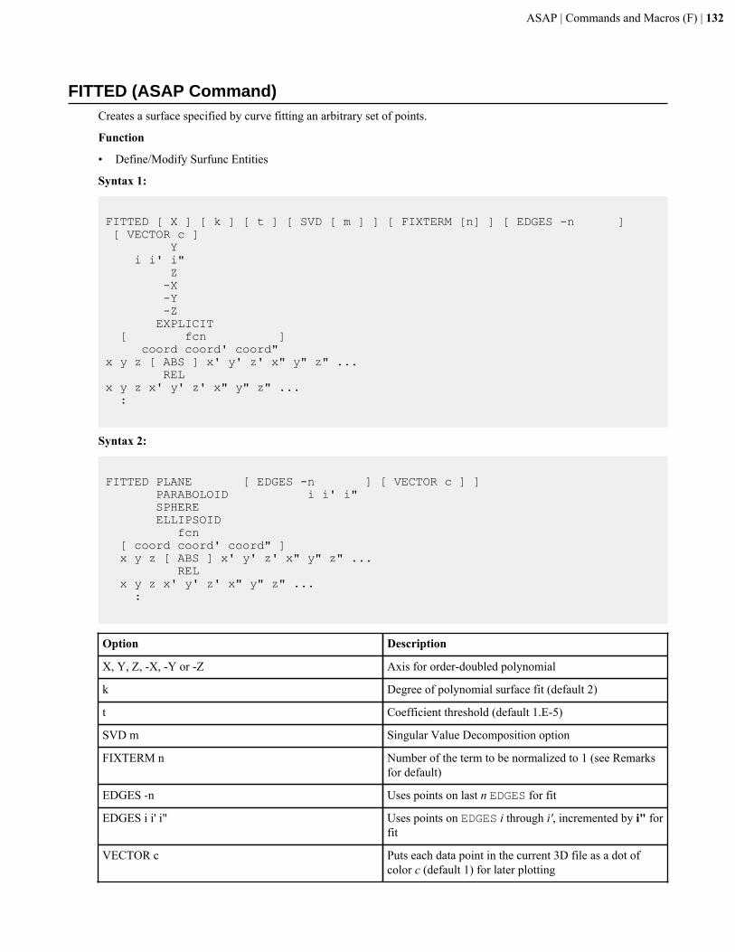
ASAP | Commands and Macros (F) | 132
FITTED (ASAP Command)Creates a surface specified by curve fitting an arbitrary set of points.
Function
• Define/Modify Surfunc Entities
Syntax 1:
FITTED [ X ] [ k ] [ t ] [ SVD [ m ] ] [ FIXTERM [n] ] [ EDGES -n ] [ VECTOR c ] Y i i' i" Z -X -Y -Z EXPLICIT [ fcn ] coord coord' coord" x y z [ ABS ] x' y' z' x" y" z" ... RELx y z x' y' z' x" y" z" ... :
Syntax 2:
FITTED PLANE [ EDGES -n ] [ VECTOR c ] ] PARABOLOID i i' i" SPHERE ELLIPSOID fcn [ coord coord' coord" ] x y z [ ABS ] x' y' z' x" y" z" ... REL x y z x' y' z' x" y" z" ... :
Option Description
X, Y, Z, -X, -Y or -Z Axis for order-doubled polynomial
k Degree of polynomial surface fit (default 2)
t Coefficient threshold (default 1.E-5)
SVD m Singular Value Decomposition option
FIXTERM n Number of the term to be normalized to 1 (see Remarksfor default)
EDGES -n Uses points on last n EDGES for fit
EDGES i i' i" Uses points on EDGES i through i', incremented by i" forfit
VECTOR c Puts each data point in the current 3D file as a dot ofcolor c (default 1) for later plotting
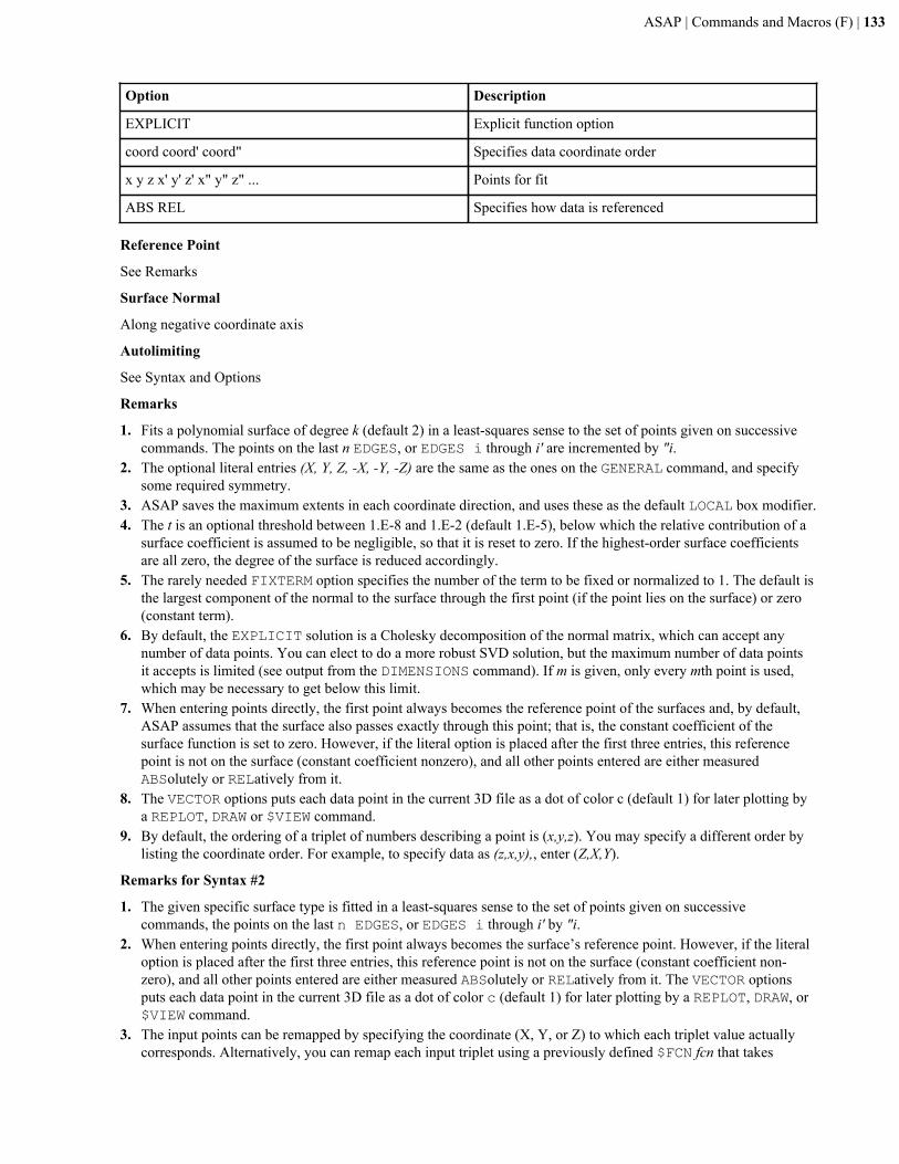
ASAP | Commands and Macros (F) | 133
Option Description
EXPLICIT Explicit function option
coord coord' coord" Specifies data coordinate order
x y z x' y' z' x" y" z" ... Points for fit
ABS REL Specifies how data is referenced
Reference Point
See Remarks
Surface Normal
Along negative coordinate axis
Autolimiting
See Syntax and Options
Remarks
1. Fits a polynomial surface of degree k (default 2) in a least-squares sense to the set of points given on successivecommands. The points on the last n EDGES, or EDGES i through i' are incremented by "i.
2. The optional literal entries (X, Y, Z, -X, -Y, -Z) are the same as the ones on the GENERAL command, and specifysome required symmetry.
3. ASAP saves the maximum extents in each coordinate direction, and uses these as the default LOCAL box modifier.4. The t is an optional threshold between 1.E-8 and 1.E-2 (default 1.E-5), below which the relative contribution of a
surface coefficient is assumed to be negligible, so that it is reset to zero. If the highest-order surface coefficientsare all zero, the degree of the surface is reduced accordingly.
5. The rarely needed FIXTERM option specifies the number of the term to be fixed or normalized to 1. The default isthe largest component of the normal to the surface through the first point (if the point lies on the surface) or zero(constant term).
6. By default, the EXPLICIT solution is a Cholesky decomposition of the normal matrix, which can accept anynumber of data points. You can elect to do a more robust SVD solution, but the maximum number of data pointsit accepts is limited (see output from the DIMENSIONS command). If m is given, only every mth point is used,which may be necessary to get below this limit.
7. When entering points directly, the first point always becomes the reference point of the surfaces and, by default,ASAP assumes that the surface also passes exactly through this point; that is, the constant coefficient of thesurface function is set to zero. However, if the literal option is placed after the first three entries, this referencepoint is not on the surface (constant coefficient nonzero), and all other points entered are either measuredABSolutely or RELatively from it.
8. The VECTOR options puts each data point in the current 3D file as a dot of color c (default 1) for later plotting bya REPLOT, DRAW or $VIEW command.
9. By default, the ordering of a triplet of numbers describing a point is (x,y,z). You may specify a different order bylisting the coordinate order. For example, to specify data as (z,x,y),, enter (Z,X,Y).
Remarks for Syntax #2
1. The given specific surface type is fitted in a least-squares sense to the set of points given on successivecommands, the points on the last n EDGES, or EDGES i through i' by "i.
2. When entering points directly, the first point always becomes the surface’s reference point. However, if the literaloption is placed after the first three entries, this reference point is not on the surface (constant coefficient non-zero), and all other points entered are either measured ABSolutely or RELatively from it. The VECTOR optionsputs each data point in the current 3D file as a dot of color c (default 1) for later plotting by a REPLOT, DRAW, or$VIEW command.
3. The input points can be remapped by specifying the coordinate (X, Y, or Z) to which each triplet value actuallycorresponds. Alternatively, you can remap each input triplet using a previously defined $FCN fcn that takes
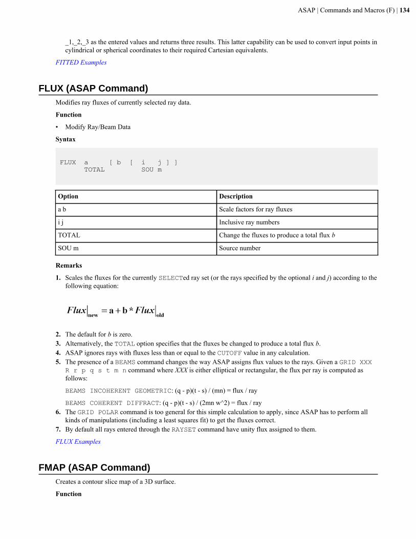
ASAP | Commands and Macros (F) | 134
_1,_2,_3 as the entered values and returns three results. This latter capability can be used to convert input points incylindrical or spherical coordinates to their required Cartesian equivalents.
FITTED Examples
FLUX (ASAP Command)Modifies ray fluxes of currently selected ray data.
Function
• Modify Ray/Beam Data
Syntax
FLUX a [ b [ i j ] ] TOTAL SOU m
Option Description
a b Scale factors for ray fluxes
i j Inclusive ray numbers
TOTAL Change the fluxes to produce a total flux b
SOU m Source number
Remarks
1. Scales the fluxes for the currently SELECTed ray set (or the rays specified by the optional i and j) according to thefollowing equation:
2. The default for b is zero.3. Alternatively, the TOTAL option specifies that the fluxes be changed to produce a total flux b.4. ASAP ignores rays with fluxes less than or equal to the CUTOFF value in any calculation.5. The presence of a BEAMS command changes the way ASAP assigns flux values to the rays. Given a GRID XXX
R r p q s t m n command where XXX is either elliptical or rectangular, the flux per ray is computed asfollows:
BEAMS INCOHERENT GEOMETRIC: (q - p)(t - s) / (mn) = flux / ray
BEAMS COHERENT DIFFRACT: (q - p)(t - s) / (2mn w^2) = flux / ray6. The GRID POLAR command is too general for this simple calculation to apply, since ASAP has to perform all
kinds of manipulations (including a least squares fit) to get the fluxes correct.7. By default all rays entered through the RAYSET command have unity flux assigned to them.
FLUX Examples
FMAP (ASAP Command)Creates a contour slice map of a 3D surface.
Function
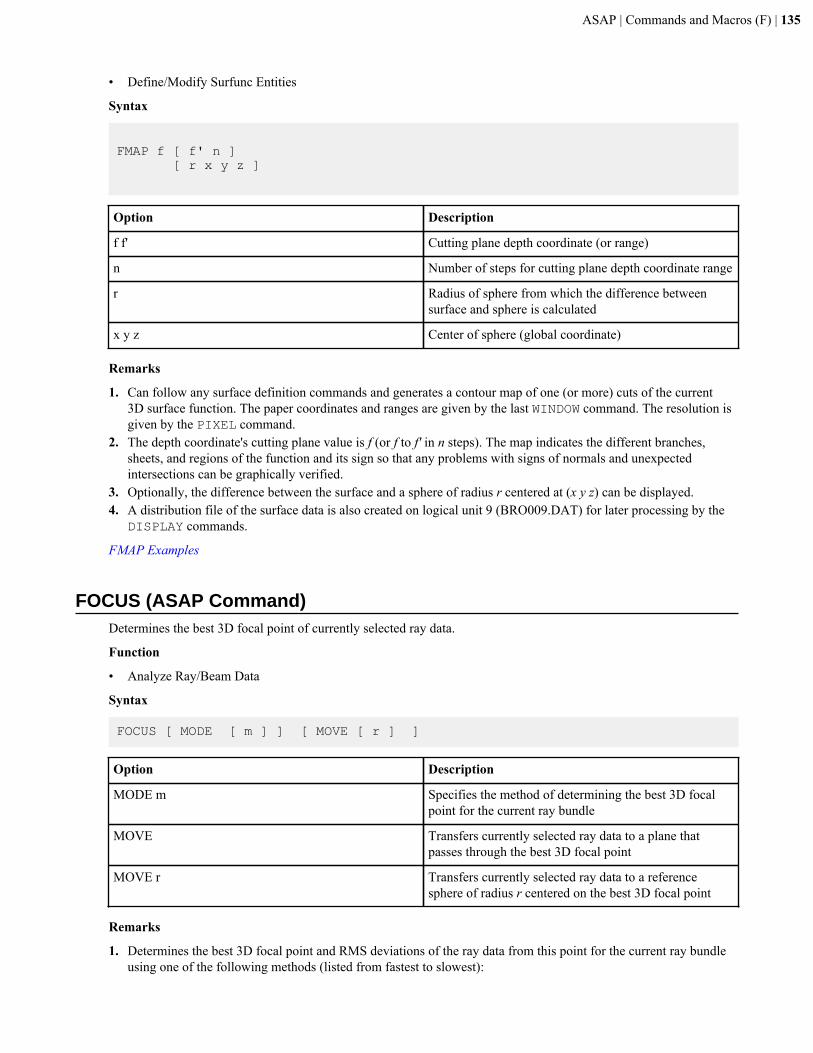
ASAP | Commands and Macros (F) | 135
• Define/Modify Surfunc Entities
Syntax
FMAP f [ f' n ] [ r x y z ]
Option Description
f f' Cutting plane depth coordinate (or range)
n Number of steps for cutting plane depth coordinate range
r Radius of sphere from which the difference betweensurface and sphere is calculated
x y z Center of sphere (global coordinate)
Remarks
1. Can follow any surface definition commands and generates a contour map of one (or more) cuts of the current3D surface function. The paper coordinates and ranges are given by the last WINDOW command. The resolution isgiven by the PIXEL command.
2. The depth coordinate's cutting plane value is f (or f to f' in n steps). The map indicates the different branches,sheets, and regions of the function and its sign so that any problems with signs of normals and unexpectedintersections can be graphically verified.
3. Optionally, the difference between the surface and a sphere of radius r centered at (x y z) can be displayed.4. A distribution file of the surface data is also created on logical unit 9 (BRO009.DAT) for later processing by the
DISPLAY commands.
FMAP Examples
FOCUS (ASAP Command)Determines the best 3D focal point of currently selected ray data.
Function
• Analyze Ray/Beam Data
Syntax
FOCUS [ MODE [ m ] ] [ MOVE [ r ] ]
Option Description
MODE m Specifies the method of determining the best 3D focalpoint for the current ray bundle
MOVE Transfers currently selected ray data to a plane thatpasses through the best 3D focal point
MOVE r Transfers currently selected ray data to a referencesphere of radius r centered on the best 3D focal point
Remarks
1. Determines the best 3D focal point and RMS deviations of the ray data from this point for the current ray bundleusing one of the following methods (listed from fastest to slowest):
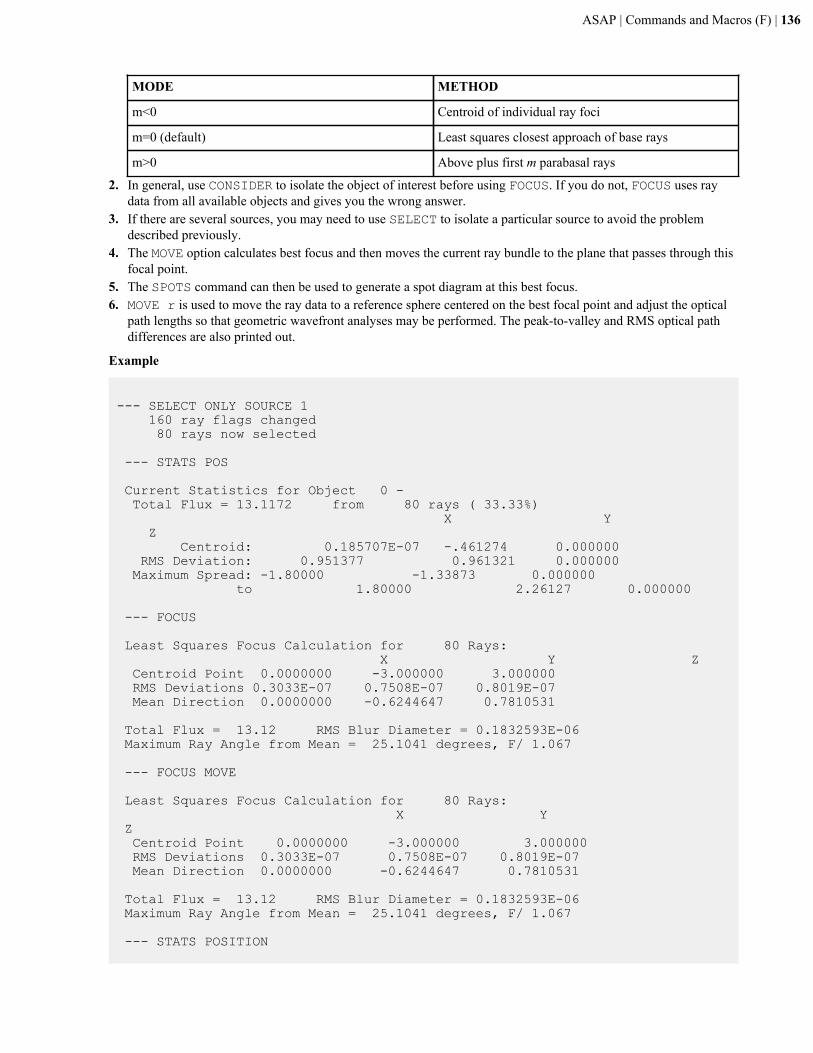
ASAP | Commands and Macros (F) | 136
MODE METHOD
m<0 Centroid of individual ray foci
m=0 (default) Least squares closest approach of base rays
m>0 Above plus first m parabasal rays
2. In general, use CONSIDER to isolate the object of interest before using FOCUS. If you do not, FOCUS uses raydata from all available objects and gives you the wrong answer.
3. If there are several sources, you may need to use SELECT to isolate a particular source to avoid the problemdescribed previously.
4. The MOVE option calculates best focus and then moves the current ray bundle to the plane that passes through thisfocal point.
5. The SPOTS command can then be used to generate a spot diagram at this best focus.6. MOVE r is used to move the ray data to a reference sphere centered on the best focal point and adjust the optical
path lengths so that geometric wavefront analyses may be performed. The peak-to-valley and RMS optical pathdifferences are also printed out.
Example
--- SELECT ONLY SOURCE 1 160 ray flags changed 80 rays now selected
--- STATS POS
Current Statistics for Object 0 - Total Flux = 13.1172 from 80 rays ( 33.33%) X Y Z Centroid: 0.185707E-07 -.461274 0.000000 RMS Deviation: 0.951377 0.961321 0.000000 Maximum Spread: -1.80000 -1.33873 0.000000 to 1.80000 2.26127 0.000000
--- FOCUS
Least Squares Focus Calculation for 80 Rays: X Y Z Centroid Point 0.0000000 -3.000000 3.000000 RMS Deviations 0.3033E-07 0.7508E-07 0.8019E-07 Mean Direction 0.0000000 -0.6244647 0.7810531
Total Flux = 13.12 RMS Blur Diameter = 0.1832593E-06 Maximum Ray Angle from Mean = 25.1041 degrees, F/ 1.067
--- FOCUS MOVE
Least Squares Focus Calculation for 80 Rays: X Y Z Centroid Point 0.0000000 -3.000000 3.000000 RMS Deviations 0.3033E-07 0.7508E-07 0.8019E-07 Mean Direction 0.0000000 -0.6244647 0.7810531
Total Flux = 13.12 RMS Blur Diameter = 0.1832593E-06 Maximum Ray Angle from Mean = 25.1041 degrees, F/ 1.067
--- STATS POSITION
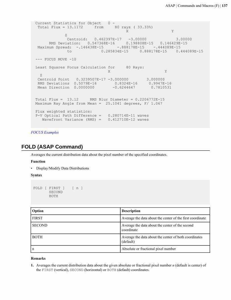
ASAP | Commands and Macros (F) | 137
Current Statistics for Object 0 - Total Flux = 13.1172 from 80 rays ( 33.33%) X Y Z Centroid: 0.462397E-17 -3.00000 3.00000 RMS Deviation: 0.547368E-16 0.198808E-15 0.146429E-15 Maximum Spread: -.146438E-15 -.888178E-15 -.444089E-15 to 0.285834E-15 0.888178E-15 0.444089E-15
--- FOCUS MOVE -10
Least Squares Focus Calculation for 80 Rays: X Y Z Centroid Point 0.3239507E-17 -3.000000 3.000000 RMS Deviations 0.5079E-16 0.8324E-16 0.9947E-16 Mean Direction 0.0000000 -0.6244647 0.7810531
Total Flux = 13.12 RMS Blur Diameter = 0.2206772E-15 Maximum Ray Angle from Mean = 25.1041 degrees, F/ 1.067
Flux weighted statistics: P-V Optical Path Difference = 0.280714E-11 waves Wavefront Variance (RMS) = 0.412710E-12 waves
FOCUS Examples
FOLD (ASAP Command)Averages the current distribution data about the pixel number of the specified coordinates.
Function
• Display/Modify Data Distributions
Syntax
FOLD [ FIRST ] [ n ] SECOND BOTH
Option Description
FIRST Average the data about the center of the first coordinate
SECOND Average the data about the center of the secondcoordinate
BOTH Average the data about the center of both coordinates(default)
n Absolute or fractional pixel number
Remarks
1. Averages the current distribution data about the given absolute or fractional pixel number n (default is center) ofthe FIRST (vertical), SECOND (horizontal) or BOTH (default) coordinates.
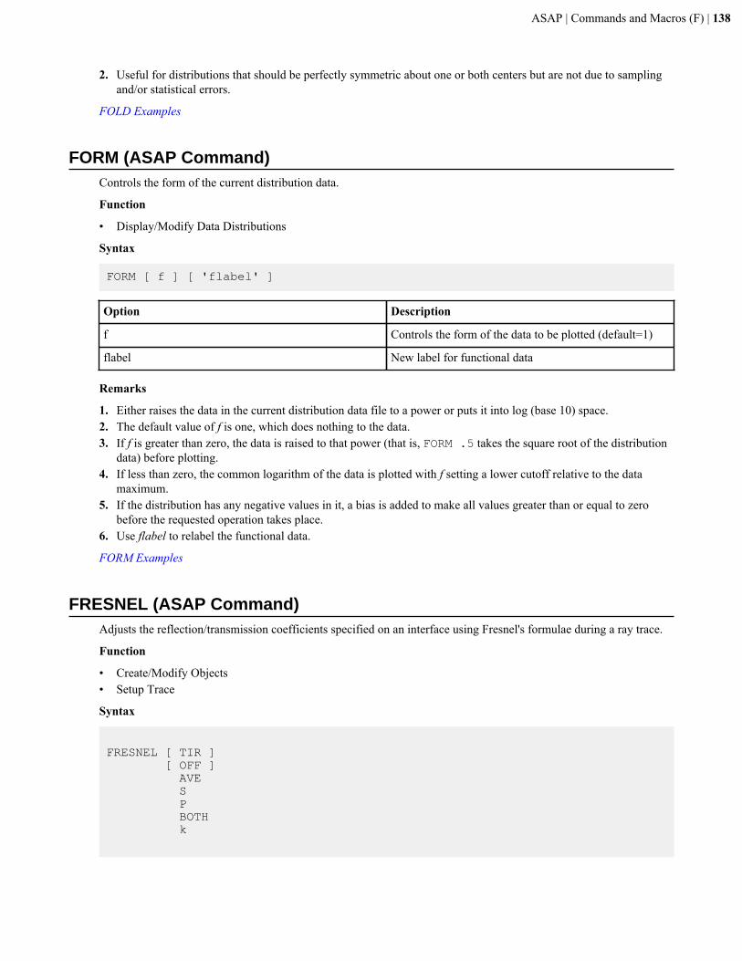
ASAP | Commands and Macros (F) | 138
2. Useful for distributions that should be perfectly symmetric about one or both centers but are not due to samplingand/or statistical errors.
FOLD Examples
FORM (ASAP Command)Controls the form of the current distribution data.
Function
• Display/Modify Data Distributions
Syntax
FORM [ f ] [ 'flabel' ]
Option Description
f Controls the form of the data to be plotted (default=1)
flabel New label for functional data
Remarks
1. Either raises the data in the current distribution data file to a power or puts it into log (base 10) space.2. The default value of f is one, which does nothing to the data.3. If f is greater than zero, the data is raised to that power (that is, FORM .5 takes the square root of the distribution
data) before plotting.4. If less than zero, the common logarithm of the data is plotted with f setting a lower cutoff relative to the data
maximum.5. If the distribution has any negative values in it, a bias is added to make all values greater than or equal to zero
before the requested operation takes place.6. Use flabel to relabel the functional data.
FORM Examples
FRESNEL (ASAP Command)Adjusts the reflection/transmission coefficients specified on an interface using Fresnel's formulae during a ray trace.
Function
• Create/Modify Objects• Setup Trace
Syntax
FRESNEL [ TIR ] [ OFF ] AVE S P BOTH k

ASAP | Commands and Macros (F) | 139
Option Description
TIR No variation with angle of incidence up to the criticalangle, then TIR
OFF No variation with angle of incidence (default)
AVE Incoherent average of polarizations
S S polarization coefficient only
P P polarization coefficient only
BOTH Both separately
k Controls which Fresnel coefficient to use in therefraction calculation
Remarks
1. This command can be used either as a local command to override defaults for the current object, or as a globalcommand. In the latter case, the command acts as an interface control and becomes the default used by any objectfor which it is not explicitly set. Since the global command is identical to the OBJECT subcommand, make sureyou are not at the OBJ> prompt when you use it as a global command. If you are, issue a RETURN command first.
2. FRESNEL is typically used with a bare coating, specified on the INTERFACE command, and a split level of oneor higher. See the topic, "Combinations of INTERFACE and FRESNEL Settings" for other settings.
3. FRESNEL can be applied globally or on an OBJECT-by-OBJECT basis, as a global modifier. One of thepolarization components of a ray is eliminated at any objects that do not have FRESNEL BOTH set.
4. Signals ASAP to take into account the variation of the reflection and transmission coefficients with incidenceangle at the object's interface and adjust the flux accordingly. It does this by evaluating the media on either side ofthe interface and then applying the Fresnel formulae.
CAUTION
• It is not possible to globally apply FRESNEL BOTH and then locally (to a specific surface, for example) applyFRESNEL OFF. The FRESNEL OFF is ignored.
• FRESNEL must be used whenever you want to recalculate the reflection/transmission coefficients for each rayduring a ray trace.
• The k parameter, or equivalent literal entry, determines which Fresnel coefficient to use in the refractioncalculation, as shown by the following:
Literal Integer k Definition
TIR -2 Allow TIR rays but no angular fluxvariation for others
OFF -1 Use normal incidence properties forall rays (default)
AVE 0 Incoherent average of polarizations
S 1 S polarization coefficient only
P 2 P polarization only
BOTH 3 Both polarizations separately
FRESNEL Examples
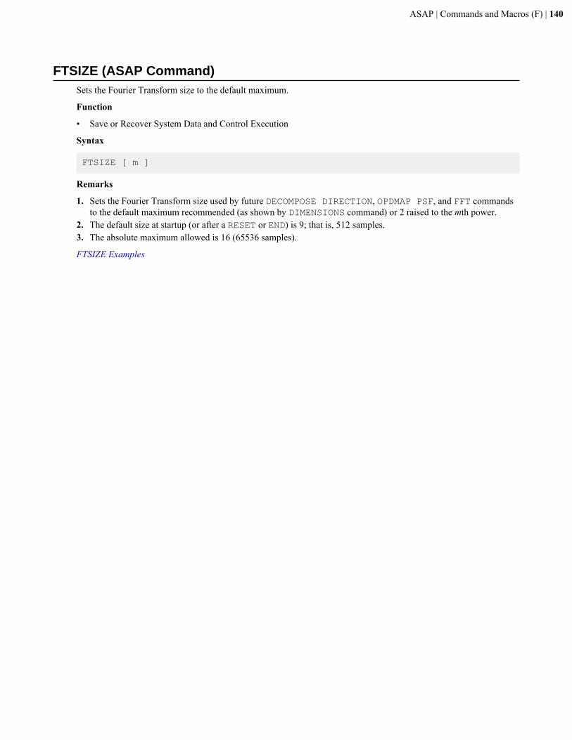
ASAP | Commands and Macros (F) | 140
FTSIZE (ASAP Command)Sets the Fourier Transform size to the default maximum.
Function
• Save or Recover System Data and Control Execution
Syntax
FTSIZE [ m ]
Remarks
1. Sets the Fourier Transform size used by future DECOMPOSE DIRECTION, OPDMAP PSF, and FFT commandsto the default maximum recommended (as shown by DIMENSIONS command) or 2 raised to the mth power.
2. The default size at startup (or after a RESET or END) is 9; that is, 512 samples.3. The absolute maximum allowed is 16 (65536 samples).
FTSIZE Examples
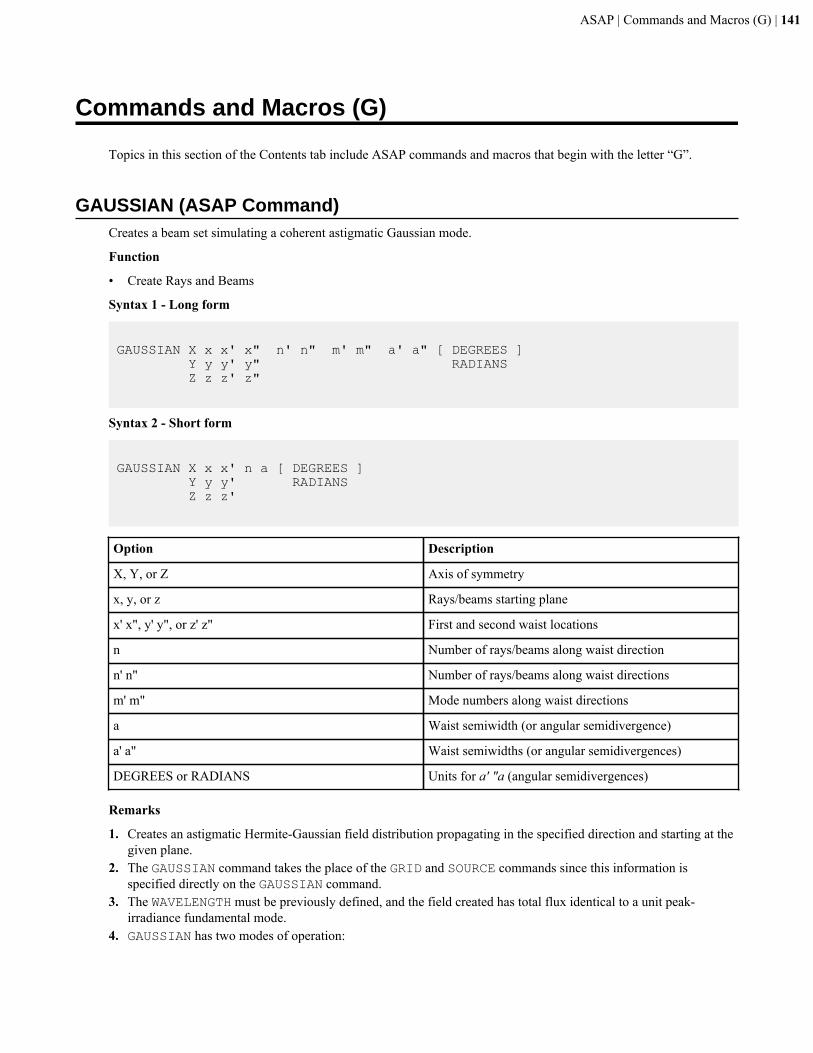
ASAP | Commands and Macros (G) | 141
Commands and Macros (G)
Topics in this section of the Contents tab include ASAP commands and macros that begin with the letter “G”.
GAUSSIAN (ASAP Command)Creates a beam set simulating a coherent astigmatic Gaussian mode.
Function
• Create Rays and Beams
Syntax 1 - Long form
GAUSSIAN X x x' x" n' n" m' m" a' a" [ DEGREES ] Y y y' y" RADIANS Z z z' z"
Syntax 2 - Short form
GAUSSIAN X x x' n a [ DEGREES ] Y y y' RADIANS Z z z'
Option Description
X, Y, or Z Axis of symmetry
x, y, or z Rays/beams starting plane
x' x", y' y", or z' z" First and second waist locations
n Number of rays/beams along waist direction
n' n" Number of rays/beams along waist directions
m' m" Mode numbers along waist directions
a Waist semiwidth (or angular semidivergence)
a' a" Waist semiwidths (or angular semidivergences)
DEGREES or RADIANS Units for a' "a (angular semidivergences)
Remarks
1. Creates an astigmatic Hermite-Gaussian field distribution propagating in the specified direction and starting at thegiven plane.
2. The GAUSSIAN command takes the place of the GRID and SOURCE commands since this information isspecified directly on the GAUSSIAN command.
3. The WAVELENGTH must be previously defined, and the field created has total flux identical to a unit peak-irradiance fundamental mode.
4. GAUSSIAN has two modes of operation:

ASAP | Commands and Macros (G) | 142
• Specify the general astigmatic properties of the GAUSSIAN beam in terms of waist locations and semiwidths(that is, a HeNe laser).
• Specify the general astigmatic properties of the GAUSSIAN beam in terms of the waist locations and angularsemidivergences (that is, a semiconductor-like laser).
5. The waist location is determined by the right-hand rule. For example, x' is the waist location (or line focus) alongthe y direction, and "x is the waist location (or line focus) along the z direction.
6. When you specify angular semidivergences, you should not have a coincident ray starting plane and waistlocations. Start the rays at a distance away from the waist locations and use the MOVE command to move the raysto the actual waist locations.
7. The current CLIP POSITION and flux CUTOFF/HALT settings may be used to truncate the rays created withthe GAUSSIAN command.
8. When the beam is in the fundamental mode, circularly symmetric, and not astigmatic, then the short form may beused.
Example
--- CF=0.8862269 --- UNITS MM --- RAYS 0 0 rays defined
--- WAVELENGTH 0.6328 UM --- PARABASAL 4; WIDTH 1.6 --- GAUSSIAN Z 0 0 0 21 21 0 0 0.4*CF 0.6*CF OVERALL Gaussian semi-widths 0.354491 0.531736 wavefront curvatures 0.000000 0.000000 Individual beam semi-widths 0.716071E-01 0.107411 ( 113.159 169.739 waves) 293 rays created in a GAUSSIAN distribution for a total 293
GAUSSIAN Examples
GENERAL (ASAP Command)Creates a general surface defined by polynomial coefficients.
Function
• Define/Modify Surfunc Entities
Syntax
GENERAL [ X ] [ x y z [ c c' c" ... ] ]COEFFICIENTS Y Z -X -Y -Z EXPLICITXiYjZk c [ c' c" ... ] :
Option Description
X, Y, Z, -X, -Y, or -Z Axis for order-doubled polynomial
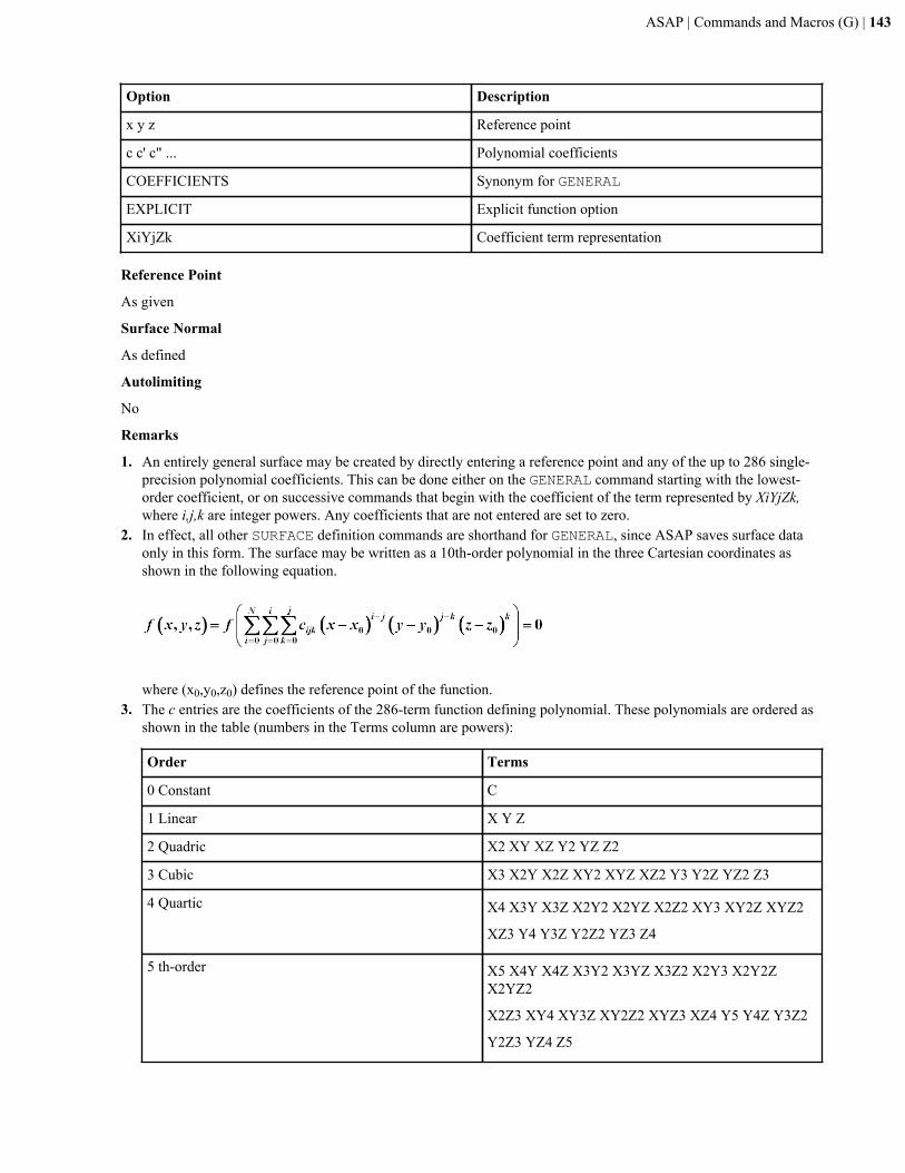
ASAP | Commands and Macros (G) | 143
Option Description
x y z Reference point
c c' c" ... Polynomial coefficients
COEFFICIENTS Synonym for GENERAL
EXPLICIT Explicit function option
XiYjZk Coefficient term representation
Reference Point
As given
Surface Normal
As defined
Autolimiting
No
Remarks
1. An entirely general surface may be created by directly entering a reference point and any of the up to 286 single-precision polynomial coefficients. This can be done either on the GENERAL command starting with the lowest-order coefficient, or on successive commands that begin with the coefficient of the term represented by XiYjZk,where i,j,k are integer powers. Any coefficients that are not entered are set to zero.
2. In effect, all other SURFACE definition commands are shorthand for GENERAL, since ASAP saves surface dataonly in this form. The surface may be written as a 10th-order polynomial in the three Cartesian coordinates asshown in the following equation.
where (x0,y0,z0) defines the reference point of the function.3. The c entries are the coefficients of the 286-term function defining polynomial. These polynomials are ordered as
shown in the table (numbers in the Terms column are powers):
Order Terms
0 Constant C
1 Linear X Y Z
2 Quadric X2 XY XZ Y2 YZ Z2
3 Cubic X3 X2Y X2Z XY2 XYZ XZ2 Y3 Y2Z YZ2 Z3
4 Quartic X4 X3Y X3Z X2Y2 X2YZ X2Z2 XY3 XY2Z XYZ2
XZ3 Y4 Y3Z Y2Z2 YZ3 Z4
5 th-order X5 X4Y X4Z X3Y2 X3YZ X3Z2 X2Y3 X2Y2ZX2YZ2
X2Z3 XY4 XY3Z XY2Z2 XYZ3 XZ4 Y5 Y4Z Y3Z2
Y2Z3 YZ4 Z5
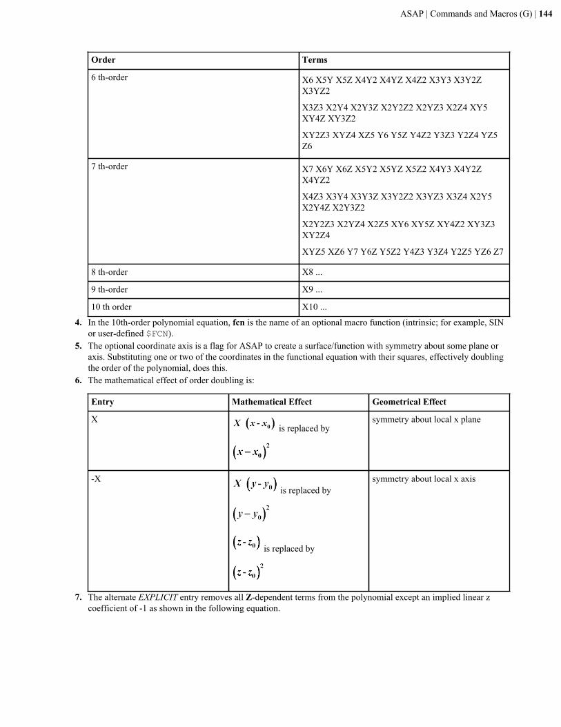
ASAP | Commands and Macros (G) | 144
Order Terms
6 th-order X6 X5Y X5Z X4Y2 X4YZ X4Z2 X3Y3 X3Y2ZX3YZ2
X3Z3 X2Y4 X2Y3Z X2Y2Z2 X2YZ3 X2Z4 XY5XY4Z XY3Z2
XY2Z3 XYZ4 XZ5 Y6 Y5Z Y4Z2 Y3Z3 Y2Z4 YZ5Z6
7 th-order X7 X6Y X6Z X5Y2 X5YZ X5Z2 X4Y3 X4Y2ZX4YZ2
X4Z3 X3Y4 X3Y3Z X3Y2Z2 X3YZ3 X3Z4 X2Y5X2Y4Z X2Y3Z2
X2Y2Z3 X2YZ4 X2Z5 XY6 XY5Z XY4Z2 XY3Z3XY2Z4
XYZ5 XZ6 Y7 Y6Z Y5Z2 Y4Z3 Y3Z4 Y2Z5 YZ6 Z7
8 th-order X8 ...
9 th-order X9 ...
10 th order X10 ...
4. In the 10th-order polynomial equation, fcn is the name of an optional macro function (intrinsic; for example, SINor user-defined $FCN).
5. The optional coordinate axis is a flag for ASAP to create a surface/function with symmetry about some plane oraxis. Substituting one or two of the coordinates in the functional equation with their squares, effectively doublingthe order of the polynomial, does this.
6. The mathematical effect of order doubling is:
Entry Mathematical Effect Geometrical Effect
X is replaced by
symmetry about local x plane
-X is replaced by
is replaced by
symmetry about local x axis
7. The alternate EXPLICIT entry removes all Z-dependent terms from the polynomial except an implied linear zcoefficient of -1 as shown in the following equation.
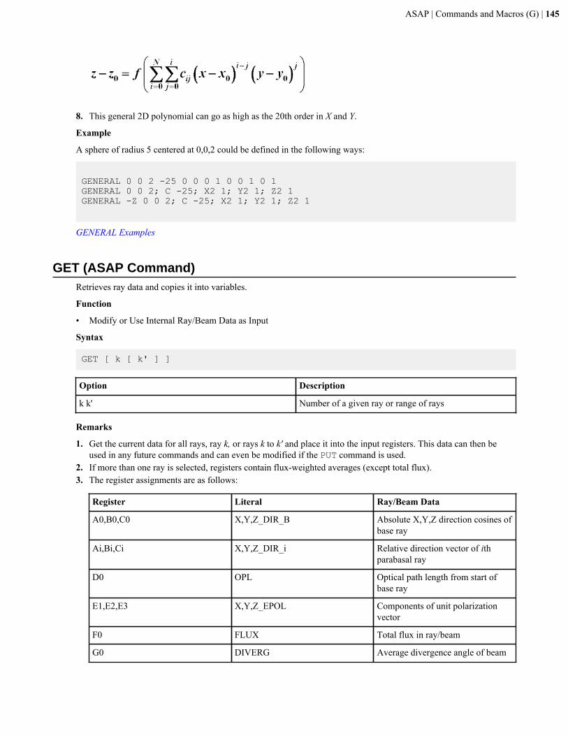
ASAP | Commands and Macros (G) | 145
8. This general 2D polynomial can go as high as the 20th order in X and Y.
Example
A sphere of radius 5 centered at 0,0,2 could be defined in the following ways:
GENERAL 0 0 2 -25 0 0 0 1 0 0 1 0 1GENERAL 0 0 2; C -25; X2 1; Y2 1; Z2 1GENERAL -Z 0 0 2; C -25; X2 1; Y2 1; Z2 1
GENERAL Examples
GET (ASAP Command)Retrieves ray data and copies it into variables.
Function
• Modify or Use Internal Ray/Beam Data as Input
Syntax
GET [ k [ k' ] ]
Option Description
k k' Number of a given ray or range of rays
Remarks
1. Get the current data for all rays, ray k, or rays k to k' and place it into the input registers. This data can then beused in any future commands and can even be modified if the PUT command is used.
2. If more than one ray is selected, registers contain flux-weighted averages (except total flux).3. The register assignments are as follows:
Register Literal Ray/Beam Data
A0,B0,C0 X,Y,Z_DIR_B Absolute X,Y,Z direction cosines ofbase ray
Ai,Bi,Ci X,Y,Z_DIR_i Relative direction vector of ithparabasal ray
D0 OPL Optical path length from start ofbase ray
E1,E2,E3 X,Y,Z_EPOL Components of unit polarizationvector
F0 FLUX Total flux in ray/beam
G0 DIVERG Average divergence angle of beam
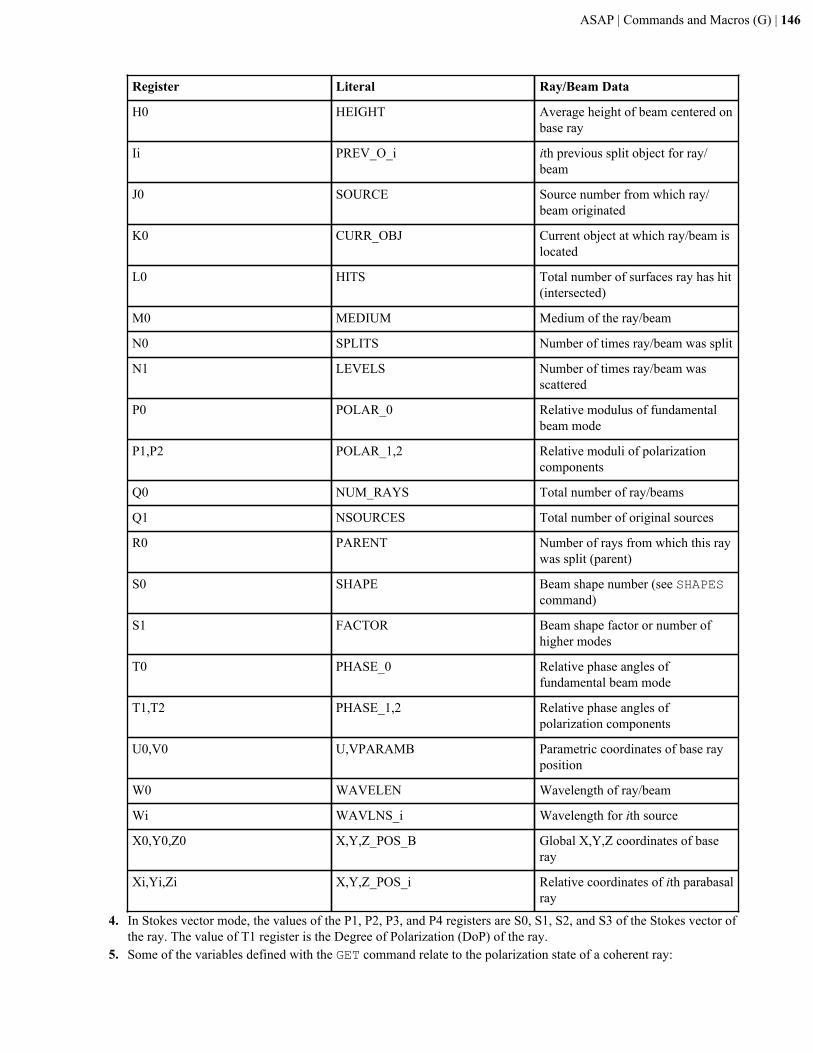
ASAP | Commands and Macros (G) | 146
Register Literal Ray/Beam Data
H0 HEIGHT Average height of beam centered onbase ray
Ii PREV_O_i ith previous split object for ray/beam
J0 SOURCE Source number from which ray/beam originated
K0 CURR_OBJ Current object at which ray/beam islocated
L0 HITS Total number of surfaces ray has hit(intersected)
M0 MEDIUM Medium of the ray/beam
N0 SPLITS Number of times ray/beam was split
N1 LEVELS Number of times ray/beam wasscattered
P0 POLAR_0 Relative modulus of fundamentalbeam mode
P1,P2 POLAR_1,2 Relative moduli of polarizationcomponents
Q0 NUM_RAYS Total number of ray/beams
Q1 NSOURCES Total number of original sources
R0 PARENT Number of rays from which this raywas split (parent)
S0 SHAPE Beam shape number (see SHAPEScommand)
S1 FACTOR Beam shape factor or number ofhigher modes
T0 PHASE_0 Relative phase angles offundamental beam mode
T1,T2 PHASE_1,2 Relative phase angles ofpolarization components
U0,V0 U,VPARAMB Parametric coordinates of base rayposition
W0 WAVELEN Wavelength of ray/beam
Wi WAVLNS_i Wavelength for ith source
X0,Y0,Z0 X,Y,Z_POS_B Global X,Y,Z coordinates of baseray
Xi,Yi,Zi X,Y,Z_POS_i Relative coordinates of ith parabasalray
4. In Stokes vector mode, the values of the P1, P2, P3, and P4 registers are S0, S1, S2, and S3 of the Stokes vector ofthe ray. The value of T1 register is the Degree of Polarization (DoP) of the ray.
5. Some of the variables defined with the GET command relate to the polarization state of a coherent ray:
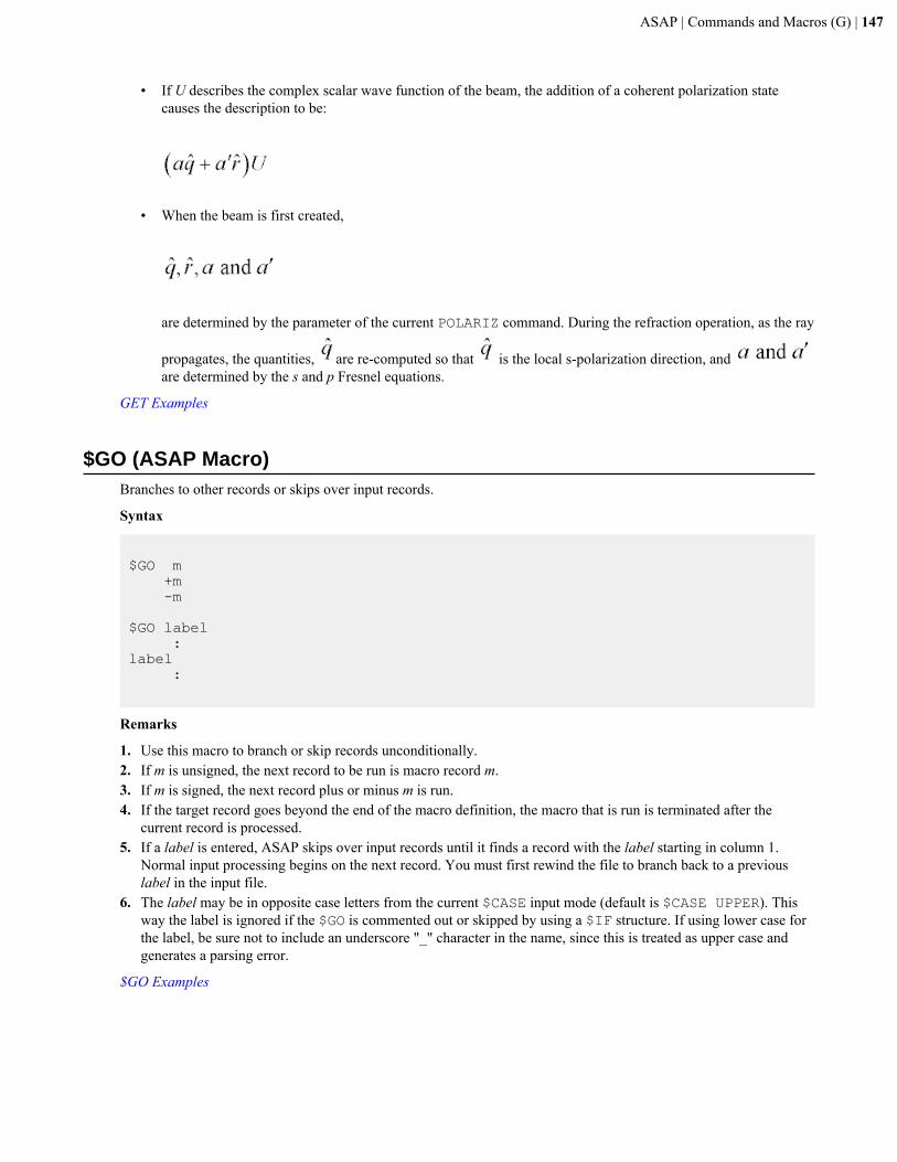
ASAP | Commands and Macros (G) | 147
• If U describes the complex scalar wave function of the beam, the addition of a coherent polarization statecauses the description to be:
• When the beam is first created,
are determined by the parameter of the current POLARIZ command. During the refraction operation, as the ray
propagates, the quantities, are re-computed so that is the local s-polarization direction, and are determined by the s and p Fresnel equations.
GET Examples
$GO (ASAP Macro)Branches to other records or skips over input records.
Syntax
$GO m +m -m
$GO label :label :
Remarks
1. Use this macro to branch or skip records unconditionally.2. If m is unsigned, the next record to be run is macro record m.3. If m is signed, the next record plus or minus m is run.4. If the target record goes beyond the end of the macro definition, the macro that is run is terminated after the
current record is processed.5. If a label is entered, ASAP skips over input records until it finds a record with the label starting in column 1.
Normal input processing begins on the next record. You must first rewind the file to branch back to a previouslabel in the input file.
6. The label may be in opposite case letters from the current $CASE input mode (default is $CASE UPPER). Thisway the label is ignored if the $GO is commented out or skipped by using a $IF structure. If using lower case forthe label, be sure not to include an underscore "_" character in the name, since this is treated as upper case andgenerates a parsing error.
$GO Examples
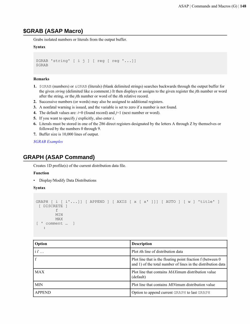
ASAP | Commands and Macros (G) | 148
$GRAB (ASAP Macro)Grabs isolated numbers or literals from the output buffer.
Syntax
$GRAB 'string' [ i j ] [ reg [ reg '...]]$GRAB
Remarks
1. $GRAB (numbers) or &GRAB (literals) (blank delimited strings) searches backwards through the output buffer forthe given string (delimited like a comment.) It then displays or assigns to the given register the jth number or wordafter the string, or the jth number or word of the ith relative record.
2. Successive numbers (or words) may also be assigned to additional registers.3. A nonfatal warning is issued, and the variable is set to zero if a number is not found.4. The default values are: i=0 (found record) and j=1 (next number or word).5. If you want to specify j explicitly, also enter i.6. Literals must be stored in one of the 286 direct registers designated by the letters A through Z by themselves or
followed by the numbers 0 through 9.7. Buffer size is 10,000 lines of output.
$GRAB Examples
GRAPH (ASAP Command)Creates 1D profile(s) of the current distribution data file.
Function
• Display/Modify Data Distributions
Syntax
GRAPH [ i [ i'...]] [ APPEND ] [ AXIS [ x [ x' ]]] [ AUTO ] [ w ] 'title' ] [ DISCRETE ] f MIN MAX[ ' comment … ] :
Option Description
i i' … Plot ith line of distribution data
f Plot line that is the floating point fraction f (between 0and 1) of the total number of lines in the distribution data
MAX Plot line that contains MAXimum distribution value(default)
MIN Plot line that contains MINimum distribution value
APPEND Option to append current GRAPH to last GRAPH
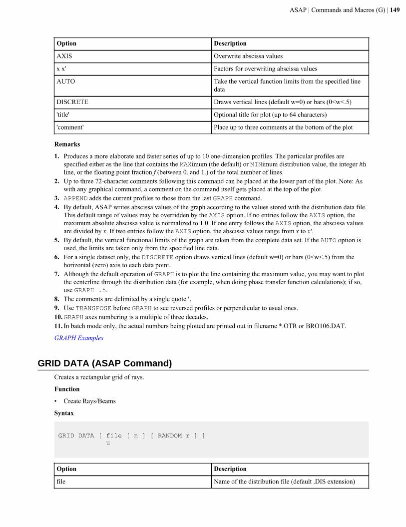
ASAP | Commands and Macros (G) | 149
Option Description
AXIS Overwrite abscissa values
x x' Factors for overwriting abscissa values
AUTO Take the vertical function limits from the specified linedata
DISCRETE Draws vertical lines (default w=0) or bars (0<w<.5)
'title' Optional title for plot (up to 64 characters)
'comment' Place up to three comments at the bottom of the plot
Remarks
1. Produces a more elaborate and faster series of up to 10 one-dimension profiles. The particular profiles arespecified either as the line that contains the MAXimum (the default) or MINimum distribution value, the integer ithline, or the floating point fraction f (between 0. and 1.) of the total number of lines.
2. Up to three 72-character comments following this command can be placed at the lower part of the plot. Note: Aswith any graphical command, a comment on the command itself gets placed at the top of the plot.
3. APPEND adds the current profiles to those from the last GRAPH command.4. By default, ASAP writes abscissa values of the graph according to the values stored with the distribution data file.
This default range of values may be overridden by the AXIS option. If no entries follow the AXIS option, themaximum absolute abscissa value is normalized to 1.0. If one entry follows the AXIS option, the abscissa valuesare divided by x. If two entries follow the AXIS option, the abscissa values range from x to x'.
5. By default, the vertical functional limits of the graph are taken from the complete data set. If the AUTO option isused, the limits are taken only from the specified line data.
6. For a single dataset only, the DISCRETE option draws vertical lines (default w=0) or bars (0<w<.5) from thehorizontal (zero) axis to each data point.
7. Although the default operation of GRAPH is to plot the line containing the maximum value, you may want to plotthe centerline through the distribution data (for example, when doing phase transfer function calculations); if so,use GRAPH .5.
8. The comments are delimited by a single quote '.9. Use TRANSPOSE before GRAPH to see reversed profiles or perpendicular to usual ones.10.GRAPH axes numbering is a multiple of three decades.11. In batch mode only, the actual numbers being plotted are printed out in filename *.OTR or BRO106.DAT.
GRAPH Examples
GRID DATA (ASAP Command)Creates a rectangular grid of rays.
Function
• Create Rays/Beams
Syntax
GRID DATA [ file [ n ] [ RANDOM r ] ] u
Option Description
file Name of the distribution file (default .DIS extension)
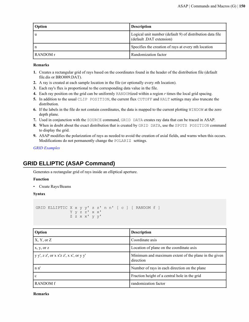
ASAP | Commands and Macros (G) | 150
Option Description
u Logical unit number (default 9) of distribution data file(default .DAT extension)
n Specifies the creation of rays at every nth location
RANDOM r Randomization factor
Remarks
1. Creates a rectangular grid of rays based on the coordinates found in the header of the distribution file (defaultfile.dis or BRO009.DAT).
2. A ray is created at each sample location in the file (or optionally every nth location).3. Each ray's flux is proportional to the corresponding data value in the file.4. Each ray position on the grid can be uniformly RANDOMized within a region r times the local grid spacing.5. In addition to the usual CLIP POSITION, the current flux CUTOFF and HALT settings may also truncate the
distribution.6. If the labels in the file do not contain coordinates, the data is mapped to the current plotting WINDOW at the zero
depth plane.7. Used in conjunction with the SOURCE command, GRID DATA creates ray data that can be traced in ASAP.8. When in doubt about the exact distribution that is created by GRID DATA, use the SPOTS POSITION command
to display the grid.9. ASAP modifies the polarization of rays as needed to avoid the creation of axial fields, and warns when this occurs.
Modifications do not permanently change the POLARIZ settings.
GRID Examples
GRID ELLIPTIC (ASAP Command)Generates a rectangular grid of rays inside an elliptical aperture.
Function
• Create Rays/Beams
Syntax
GRID ELLIPTIC X x y y' z z' n n' [ c ] [ RANDOM f ] Y y z z' x x' Z z x x' y y'
Option Description
X, Y, or Z Coordinate axis
x, y, or z Location of plane on the coordinate axis
y y', z z', or x x'z z', x x', or y y' Minimum and maximum extent of the plane in the givendirection
n n' Number of rays in each direction on the plane
c Fraction height of a central hole in the grid
RANDOM f randomization factor
Remarks
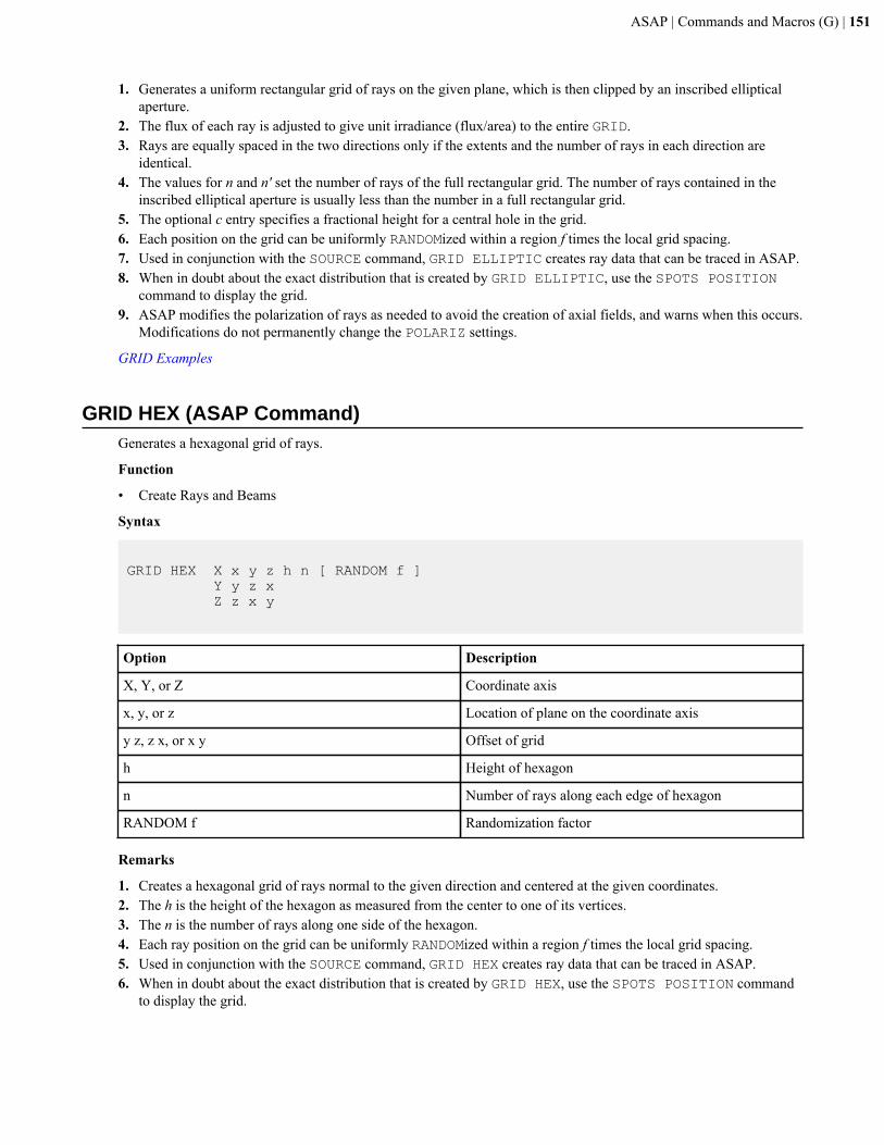
ASAP | Commands and Macros (G) | 151
1. Generates a uniform rectangular grid of rays on the given plane, which is then clipped by an inscribed ellipticalaperture.
2. The flux of each ray is adjusted to give unit irradiance (flux/area) to the entire GRID.3. Rays are equally spaced in the two directions only if the extents and the number of rays in each direction are
identical.4. The values for n and n' set the number of rays of the full rectangular grid. The number of rays contained in the
inscribed elliptical aperture is usually less than the number in a full rectangular grid.5. The optional c entry specifies a fractional height for a central hole in the grid.6. Each position on the grid can be uniformly RANDOMized within a region f times the local grid spacing.7. Used in conjunction with the SOURCE command, GRID ELLIPTIC creates ray data that can be traced in ASAP.8. When in doubt about the exact distribution that is created by GRID ELLIPTIC, use the SPOTS POSITION
command to display the grid.9. ASAP modifies the polarization of rays as needed to avoid the creation of axial fields, and warns when this occurs.
Modifications do not permanently change the POLARIZ settings.
GRID Examples
GRID HEX (ASAP Command)Generates a hexagonal grid of rays.
Function
• Create Rays and Beams
Syntax
GRID HEX X x y z h n [ RANDOM f ] Y y z x Z z x y
Option Description
X, Y, or Z Coordinate axis
x, y, or z Location of plane on the coordinate axis
y z, z x, or x y Offset of grid
h Height of hexagon
n Number of rays along each edge of hexagon
RANDOM f Randomization factor
Remarks
1. Creates a hexagonal grid of rays normal to the given direction and centered at the given coordinates.2. The h is the height of the hexagon as measured from the center to one of its vertices.3. The n is the number of rays along one side of the hexagon.4. Each ray position on the grid can be uniformly RANDOMized within a region f times the local grid spacing.5. Used in conjunction with the SOURCE command, GRID HEX creates ray data that can be traced in ASAP.6. When in doubt about the exact distribution that is created by GRID HEX, use the SPOTS POSITION command
to display the grid.
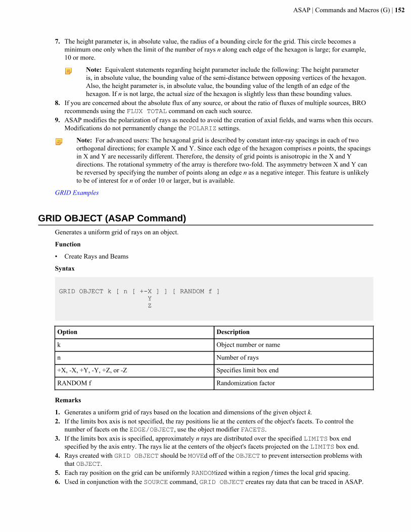
ASAP | Commands and Macros (G) | 152
7. The height parameter is, in absolute value, the radius of a bounding circle for the grid. This circle becomes aminimum one only when the limit of the number of rays n along each edge of the hexagon is large; for example,10 or more.
Note: Equivalent statements regarding height parameter include the following: The height parameteris, in absolute value, the bounding value of the semi-distance between opposing vertices of the hexagon.Also, the height parameter is, in absolute value, the bounding value of the length of an edge of thehexagon. If n is not large, the actual size of the hexagon is slightly less than these bounding values.
8. If you are concerned about the absolute flux of any source, or about the ratio of fluxes of multiple sources, BROrecommends using the FLUX TOTAL command on each such source.
9. ASAP modifies the polarization of rays as needed to avoid the creation of axial fields, and warns when this occurs.Modifications do not permanently change the POLARIZ settings.
Note: For advanced users: The hexagonal grid is described by constant inter-ray spacings in each of twoorthogonal directions; for example X and Y. Since each edge of the hexagon comprises n points, the spacingsin X and Y are necessarily different. Therefore, the density of grid points is anisotropic in the X and Ydirections. The rotational symmetry of the array is therefore two-fold. The asymmetry between X and Y canbe reversed by specifying the number of points along an edge n as a negative integer. This feature is unlikelyto be of interest for n of order 10 or larger, but is available.
GRID Examples
GRID OBJECT (ASAP Command)Generates a uniform grid of rays on an object.
Function
• Create Rays and Beams
Syntax
GRID OBJECT k [ n [ +-X ] ] [ RANDOM f ] Y Z
Option Description
k Object number or name
n Number of rays
+X, -X, +Y, -Y, +Z, or -Z Specifies limit box end
RANDOM f Randomization factor
Remarks
1. Generates a uniform grid of rays based on the location and dimensions of the given object k.2. If the limits box axis is not specified, the ray positions lie at the centers of the object's facets. To control the
number of facets on the EDGE/OBJECT, use the object modifier FACETS.3. If the limits box axis is specified, approximately n rays are distributed over the specified LIMITS box end
specified by the axis entry. The rays lie at the centers of the object's facets projected on the LIMITS box end.4. Rays created with GRID OBJECT should be MOVEd off of the OBJECT to prevent intersection problems with
that OBJECT.5. Each ray position on the grid can be uniformly RANDOMized within a region f times the local grid spacing.6. Used in conjunction with the SOURCE command, GRID OBJECT creates ray data that can be traced in ASAP.
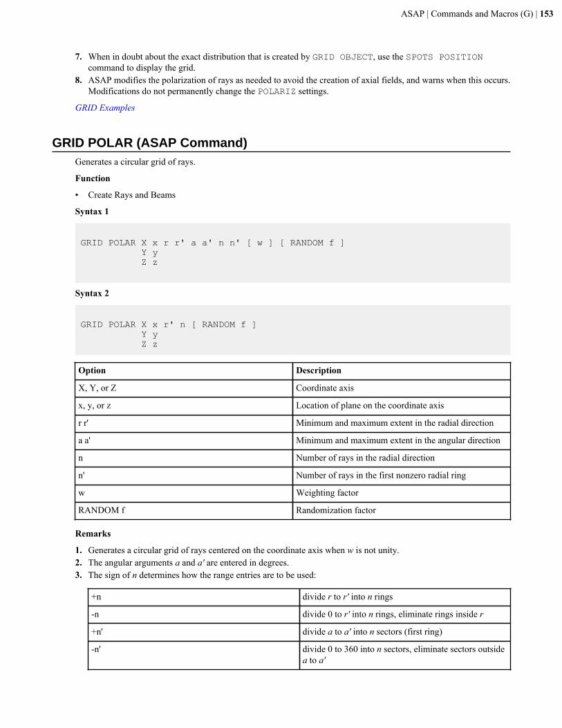
ASAP | Commands and Macros (G) | 153
7. When in doubt about the exact distribution that is created by GRID OBJECT, use the SPOTS POSITIONcommand to display the grid.
8. ASAP modifies the polarization of rays as needed to avoid the creation of axial fields, and warns when this occurs.Modifications do not permanently change the POLARIZ settings.
GRID Examples
GRID POLAR (ASAP Command)Generates a circular grid of rays.
Function
• Create Rays and Beams
Syntax 1
GRID POLAR X x r r' a a' n n' [ w ] [ RANDOM f ] Y y Z z
Syntax 2
GRID POLAR X x r' n [ RANDOM f ] Y y Z z
Option Description
X, Y, or Z Coordinate axis
x, y, or z Location of plane on the coordinate axis
r r' Minimum and maximum extent in the radial direction
a a' Minimum and maximum extent in the angular direction
n Number of rays in the radial direction
n' Number of rays in the first nonzero radial ring
w Weighting factor
RANDOM f Randomization factor
Remarks
1. Generates a circular grid of rays centered on the coordinate axis when w is not unity.2. The angular arguments a and a' are entered in degrees.3. The sign of n determines how the range entries are to be used:
+n divide r to r' into n rings
-n divide 0 to r' into n rings, eliminate rings inside r
+n' divide a to a' into n sectors (first ring)
-n' divide 0 to 360 into n sectors, eliminate sectors outsidea to a'

ASAP | Commands and Macros (G) | 154
4. For r=0 or n<0, the rays are distributed radially according to the formula R(i) = r'(i/n)^w.5. The rays are distributed evenly in the angular direction. The number in each ring is chosen so that all rays
represent an equal area on the plane. Therefore, when w=1 (the default), the grid is equi-polar; when w=.5, the gridis a standard straight spokes distribution.
6. If r is equal to zero, there is a ray/beam at the center of the grid.7. The flux of each ray is adjusted to give unit irradiance (flux/area) to the entire grid. GRID POLAR (in the final
sequence) in coherent mode, using a central hole, does not produce an irradiance of near 1, but actually muchhigher.
8. Each ray position on the grid can be uniformly RANDOMized within a region f times the local grid spacing.9. The second syntax is an alternate shorter form is available that creates a full circular (of radius r') hexapolar grid
(with n rings):
GRID POLAR X x r' n [ RANDOM f ] Y y Z z
10. Only a rotationally symmetric apodization may be entered with APODIZE.11. Used in conjunction with the SOURCE command, GRID POLAR creates ray data that can be traced in ASAP.12. When in doubt about the exact distribution that is created by GRID POLAR, use the SPOTS POSITION
command to display the grid.13. ASAP modifies the polarization of rays as needed to avoid the creation of axial fields, and warns when this occurs.
Modifications do not permanently change the POLARIZ settings.
GRID Examples
GRID RECT (ASAP Command)Generates a rectangular grid of rays inside a rectangular aperture.
Function
• Create Rays and Beams
Syntax
GRID RECT X x y y' z z' n n' [ c ] [ RANDOM f ] Y y z z' x x' Z z x x' y y'
Option Description
X, Y, or Z Coordinate axis
x, y, or z Location of plane on the coordinate axis
y y', z z', or x x'z z', x x', or y y' Minimum and maximum extent of the plane in the givendirection
n n' Number of rays in each direction on the plane
c Fraction height of a central hole in the grid
RANDOM f Randomization factor
Remarks
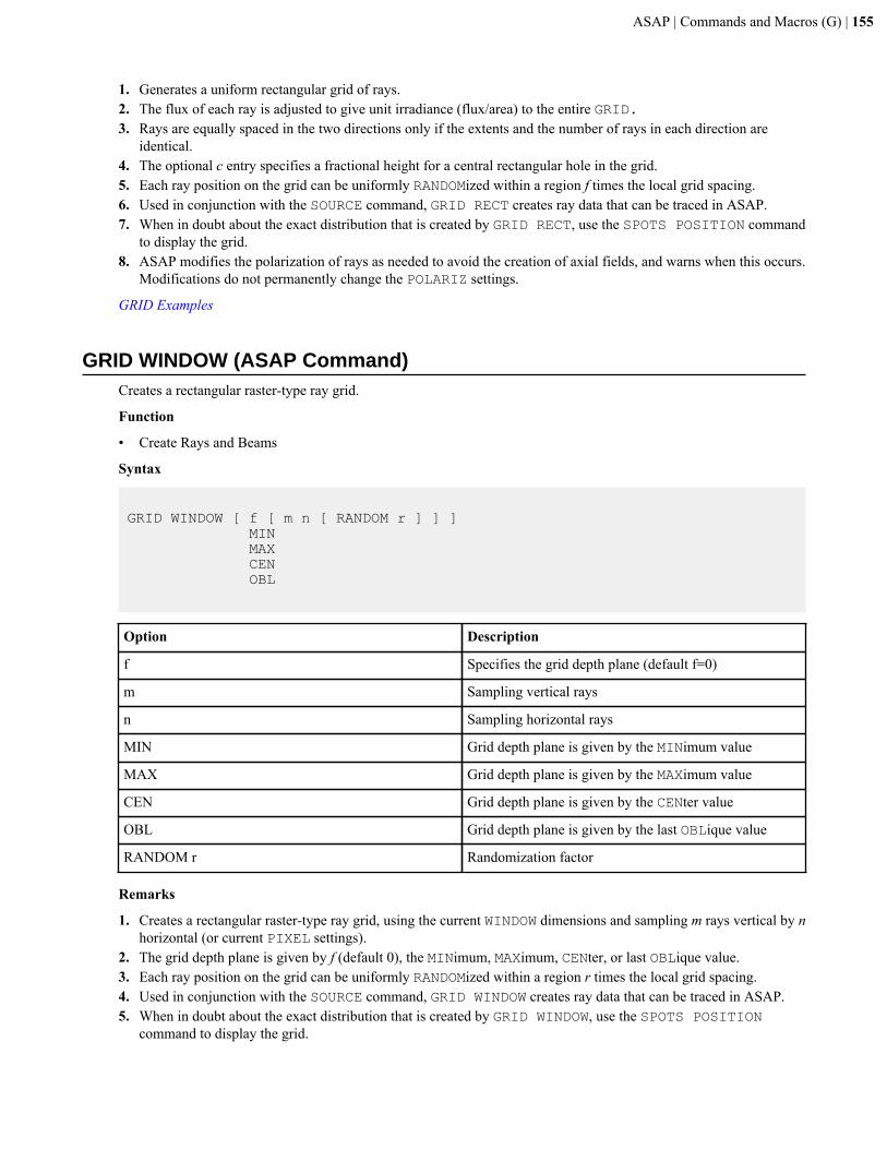
ASAP | Commands and Macros (G) | 155
1. Generates a uniform rectangular grid of rays.2. The flux of each ray is adjusted to give unit irradiance (flux/area) to the entire GRID.3. Rays are equally spaced in the two directions only if the extents and the number of rays in each direction are
identical.4. The optional c entry specifies a fractional height for a central rectangular hole in the grid.5. Each ray position on the grid can be uniformly RANDOMized within a region f times the local grid spacing.6. Used in conjunction with the SOURCE command, GRID RECT creates ray data that can be traced in ASAP.7. When in doubt about the exact distribution that is created by GRID RECT, use the SPOTS POSITION command
to display the grid.8. ASAP modifies the polarization of rays as needed to avoid the creation of axial fields, and warns when this occurs.
Modifications do not permanently change the POLARIZ settings.
GRID Examples
GRID WINDOW (ASAP Command)Creates a rectangular raster-type ray grid.
Function
• Create Rays and Beams
Syntax
GRID WINDOW [ f [ m n [ RANDOM r ] ] ] MIN MAX CEN OBL
Option Description
f Specifies the grid depth plane (default f=0)
m Sampling vertical rays
n Sampling horizontal rays
MIN Grid depth plane is given by the MINimum value
MAX Grid depth plane is given by the MAXimum value
CEN Grid depth plane is given by the CENter value
OBL Grid depth plane is given by the last OBLique value
RANDOM r Randomization factor
Remarks
1. Creates a rectangular raster-type ray grid, using the current WINDOW dimensions and sampling m rays vertical by nhorizontal (or current PIXEL settings).
2. The grid depth plane is given by f (default 0), the MINimum, MAXimum, CENter, or last OBLique value.3. Each ray position on the grid can be uniformly RANDOMized within a region r times the local grid spacing.4. Used in conjunction with the SOURCE command, GRID WINDOW creates ray data that can be traced in ASAP.5. When in doubt about the exact distribution that is created by GRID WINDOW, use the SPOTS POSITION
command to display the grid.
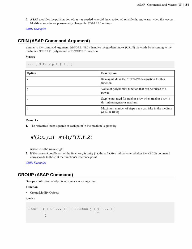
ASAP | Commands and Macros (G) | 156
6. ASAP modifies the polarization of rays as needed to avoid the creation of axial fields, and warns when this occurs.Modifications do not permanently change the POLARIZ settings.
GRID Examples
GRIN (ASAP Command Argument)Similar to the command argument, ABSORB, GRIN handles the gradient index (GRIN) materials by assigning to themedium a GENERAL polynomial or USERFUNC function.
Syntax
... [ GRIN k p t [ l ] ]
Option Description
k Its magnitude is the SURFACE designation for thisfunction
p Value of polynomial function that can be raised to apower
t Step length used for tracing a ray when tracing a ray inthis inhomogeneous medium
l Maximum number of steps a ray can take in the medium(default 1000)
Remarks
1. The refractive index squared at each point in the medium is given by:
where w is the wavelength.2. If the constant coefficient of the function f is unity (1), the refractive indices entered after the MEDIA command
corresponds to those at the function’s reference point.
GRIN Examples
GROUP (ASAP Command)Groups a collection of objects or sources as a single unit.
Function
• Create/Modify Objects
Syntax
GROUP [ i [ i' ... ] ] [ SOURCES j [ j' ... ] ] -n -n 0
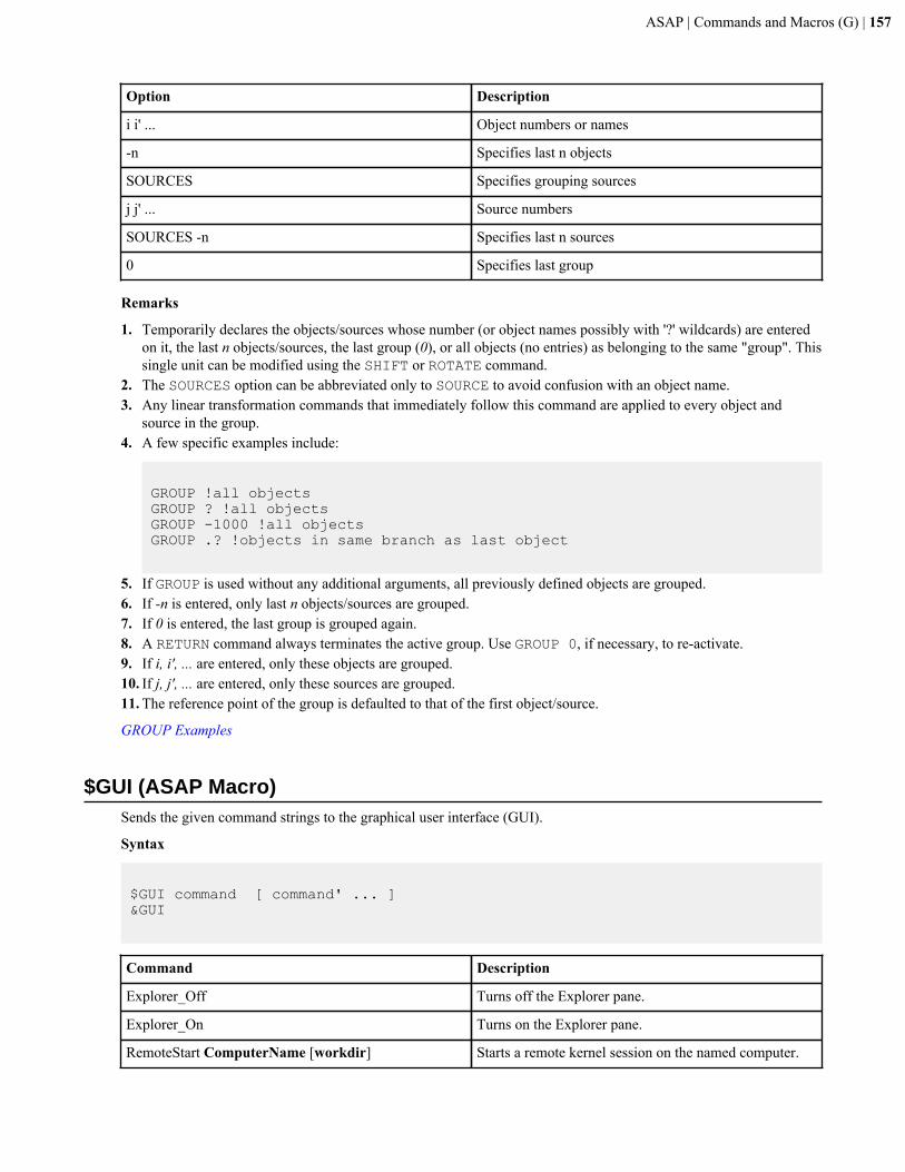
ASAP | Commands and Macros (G) | 157
Option Description
i i' ... Object numbers or names
-n Specifies last n objects
SOURCES Specifies grouping sources
j j' ... Source numbers
SOURCES -n Specifies last n sources
0 Specifies last group
Remarks
1. Temporarily declares the objects/sources whose number (or object names possibly with '?' wildcards) are enteredon it, the last n objects/sources, the last group (0), or all objects (no entries) as belonging to the same "group". Thissingle unit can be modified using the SHIFT or ROTATE command.
2. The SOURCES option can be abbreviated only to SOURCE to avoid confusion with an object name.3. Any linear transformation commands that immediately follow this command are applied to every object and
source in the group.4. A few specific examples include:
GROUP !all objectsGROUP ? !all objectsGROUP -1000 !all objectsGROUP .? !objects in same branch as last object
5. If GROUP is used without any additional arguments, all previously defined objects are grouped.6. If -n is entered, only last n objects/sources are grouped.7. If 0 is entered, the last group is grouped again.8. A RETURN command always terminates the active group. Use GROUP 0, if necessary, to re-activate.9. If i, i', ... are entered, only these objects are grouped.10. If j, j', ... are entered, only these sources are grouped.11. The reference point of the group is defaulted to that of the first object/source.
GROUP Examples
$GUI (ASAP Macro)Sends the given command strings to the graphical user interface (GUI).
Syntax
$GUI command [ command' ... ]&GUI
Command Description
Explorer_Off Turns off the Explorer pane.
Explorer_On Turns on the Explorer pane.
RemoteStart ComputerName [workdir] Starts a remote kernel session on the named computer.
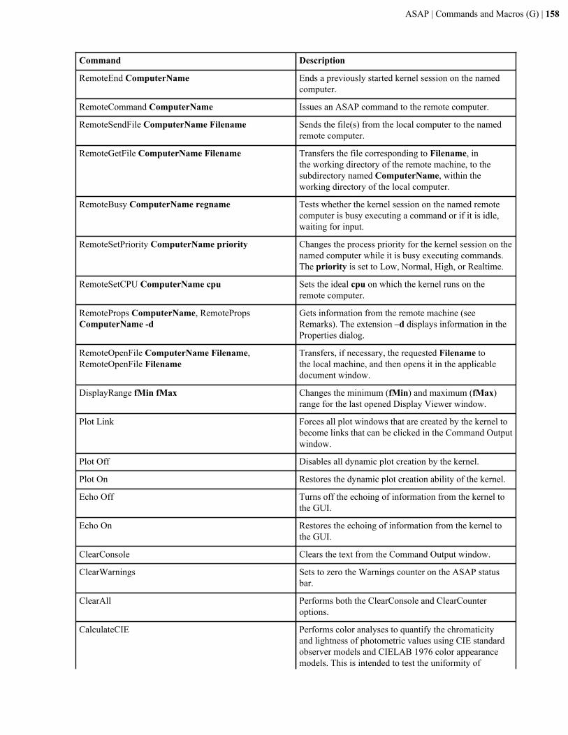
ASAP | Commands and Macros (G) | 158
Command Description
RemoteEnd ComputerName Ends a previously started kernel session on the namedcomputer.
RemoteCommand ComputerName Issues an ASAP command to the remote computer.
RemoteSendFile ComputerName Filename Sends the file(s) from the local computer to the namedremote computer.
RemoteGetFile ComputerName Filename Transfers the file corresponding to Filename, inthe working directory of the remote machine, to thesubdirectory named ComputerName, within theworking directory of the local computer.
RemoteBusy ComputerName regname Tests whether the kernel session on the named remotecomputer is busy executing a command or if it is idle,waiting for input.
RemoteSetPriority ComputerName priority Changes the process priority for the kernel session on thenamed computer while it is busy executing commands.The priority is set to Low, Normal, High, or Realtime.
RemoteSetCPU ComputerName cpu Sets the ideal cpu on which the kernel runs on theremote computer.
RemoteProps ComputerName, RemotePropsComputerName -d
Gets information from the remote machine (seeRemarks). The extension –d displays information in theProperties dialog.
RemoteOpenFile ComputerName Filename,RemoteOpenFile Filename
Transfers, if necessary, the requested Filename tothe local machine, and then opens it in the applicabledocument window.
DisplayRange fMin fMax Changes the minimum (fMin) and maximum (fMax)range for the last opened Display Viewer window.
Plot Link Forces all plot windows that are created by the kernel tobecome links that can be clicked in the Command Outputwindow.
Plot Off Disables all dynamic plot creation by the kernel.
Plot On Restores the dynamic plot creation ability of the kernel.
Echo Off Turns off the echoing of information from the kernel tothe GUI.
Echo On Restores the echoing of information from the kernel tothe GUI.
ClearConsole Clears the text from the Command Output window.
ClearWarnings Sets to zero the Warnings counter on the ASAP statusbar.
ClearAll Performs both the ClearConsole and ClearCounteroptions.
CalculateCIE Performs color analyses to quantify the chromaticityand lightness of photometric values using CIE standardobserver models and CIELAB 1976 color appearancemodels. This is intended to test the uniformity of
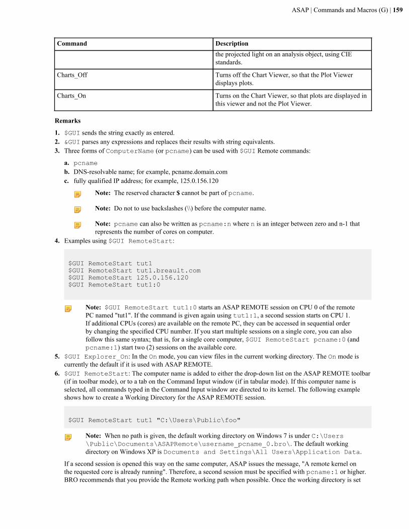
ASAP | Commands and Macros (G) | 159
Command Descriptionthe projected light on an analysis object, using CIEstandards.
Charts_Off Turns off the Chart Viewer, so that the Plot Viewerdisplays plots.
Charts_On Turns on the Chart Viewer, so that plots are displayed inthis viewer and not the Plot Viewer.
Remarks
1. $GUI sends the string exactly as entered.2. &GUI parses any expressions and replaces their results with string equivalents.3. Three forms of ComputerName (or pcname) can be used with $GUI Remote commands:
a. pcnameb. DNS-resolvable name; for example, pcname.domain.comc. fully qualified IP address; for example, 125.0.156.120
Note: The reserved character $ cannot be part of pcname.
Note: Do not to use backslashes (\\) before the computer name.
Note: pcname can also be written as pcname:n where n is an integer between zero and n-1 thatrepresents the number of cores on computer.
4. Examples using $GUI RemoteStart:
$GUI RemoteStart tut1$GUI RemoteStart tut1.breault.com$GUI RemoteStart 125.0.156.120$GUI RemoteStart tut1:0
Note: $GUI RemoteStart tut1:0 starts an ASAP REMOTE session on CPU 0 of the remotePC named "tut1". If the command is given again using tut1:1, a second session starts on CPU 1.If additional CPUs (cores) are available on the remote PC, they can be accessed in sequential orderby changing the specified CPU number. If you start multiple sessions on a single core, you can alsofollow this same syntax; that is, for a single core computer, $GUI RemoteStart pcname:0 (andpcname:1) start two (2) sessions on the available core.
5. $GUI Explorer_On: In the On mode, you can view files in the current working directory. The On mode iscurrently the default if it is used with ASAP REMOTE.
6. $GUI RemoteStart: The computer name is added to either the drop-down list on the ASAP REMOTE toolbar(if in toolbar mode), or to a tab on the Command Input window (if in tabular mode). If this computer name isselected, all commands typed in the Command Input window are directed to its kernel. The following exampleshows how to create a Working Directory for the ASAP REMOTE session.
$GUI RemoteStart tut1 "C:\Users\Public\foo"
Note: When no path is given, the default working directory on Windows 7 is under C:\Users\Public\Documents\ASAPRemote\username_pcname_0.bro\. The default workingdirectory on Windows XP is Documents and Settings\All Users\Application Data.
If a second session is opened this way on the same computer, ASAP issues the message, "A remote kernel onthe requested core is already running". Therefore, a second session must be specified with pcname:1 or higher.BRO recommends that you provide the Remote working path when possible. Once the working directory is set
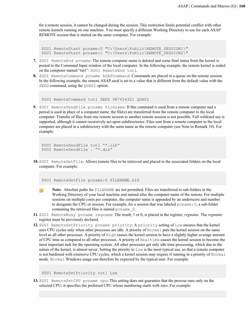
ASAP | Commands and Macros (G) | 160
for a remote session, it cannot be changed during the session. This restriction limits potential conflict with otherremote kernels running on one machine. You must specify a different Working Directory to use for each ASAPREMOTE session that is started on the same computer. For example:
$GUI RemoteStart pcname:0 "C:\Users\Public\REMOTE_SESSION1\" $GUI RemoteStart pcname:1 "C:\Users\Public\REMOTE_SESSION2\"
7. $GUI RemoteEnd pcname: The remote computer name is deleted and some final status from the kernel isposted to the Command Input window of the local computer. In the following example, the remote kernel is endedon the computer named “tut1”: $GUI RemoteEnd tut1.
8. $GUI RemoteCommand pcname ASAPCommand: Commands are placed in a queue on the remote session.In the following example, the remote ASAP seed is set to a value that is different from the default value with theSEED command, using the QUASI option:
$GUI RemoteCommand tut1 SEED 987654321 QUASI
9. $GUI RemoteSendFile pcname Filename: If this command is used from a remote computer and aperiod is used in place of a computer name, the file(s) are transferred from the remote computer to the localcomputer. Transfer of files from one remote session to another remote session is not possible. Full wildcard use issupported, although it cannot recursively act upon subdirectories. Files sent from a remote computer to the localcomputer are placed in a subdirectory with the same name as the remote computer (see Note in Remark 10). Forexample:
$GUI RemoteSendFile tut1 “*.lib”$GUI RemoteSendFile . “*.dis”
10.$GUI RemoteGetFile: Allows remote files to be retrieved and placed in the associated folders on the localcomputer. For example:
$GUI RemoteGetFile pcname:0 FILENAME.DIS
Note: Absolute paths for FILENAME are not permitted. Files are transferred to sub-folders in theWorking Directory of your local machine and named after the computer name of the remote. For multiplesessions on multiple cores per computer, the computer name is appended by an underscore and numberto designate the CPU or session. For example, for a session that was labeled pcname:0, a sub-foldercontaining the retrieved files is named pcname_0.
11.$GUI RemoteBusy pcname regname: The result, 1 or 0, is placed in the register, regname. The regnameregister must be previously declared.
12.$GUI RemoteSetPriority pcname priority: A priority setting of Low ensures that the kerneluses CPU cycles only when other processes are idle. A priority of Normal puts the kernel session on the samelevel as all other processes. A priority of High causes the kernel session to have a slightly higher average amountof CPU time as compared to all other processes. A priority of Realtime causes the kernel session to become themost important task for the operating system. All other processes get only idle time processing, which due to thenature of the kernel, is almost never. Setting the priority to Low is the most typical use, so that a remote computeris not burdened with extensive CPU cycles, which a kernel session may require if running in a priority of Normalmode. Normal Windows usage can therefore be expected by the typical user. For example:
$GUI RemoteSetPriority tut1 Low
13.$GUI RemoteSetCPU pcname cpu: This setting does not guarantee that the process runs only on theselected CPU; it specifies the preferred CPU whose numbering starts with zero. For example:
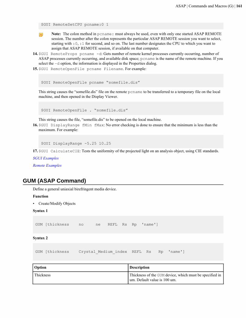
ASAP | Commands and Macros (G) | 161
$GUI RemoteSetCPU pcname:0 1
Note: The colon method in pcname: must always be used, even with only one started ASAP REMOTEsession. The number after the colon represents the particular ASAP REMOTE session you want to select,starting with :0, :1 for second, and so on. The last number designates the CPU to which you want toassign that ASAP REMOTE session, if available on that computer.
14.$GUI RemoteProps pcname -d: Gets number of remote kernel processes currently occurring, number ofASAP processes currently occurring, and available disk space; pcname is the name of the remote machine. If youselect the –d option, the information is displayed in the Properties dialog.
15.$GUI RemoteOpenFile pcname Filename. For example:
$GUI RemoteOpenFile pcname “somefile.dis”
This string causes the “somefile.dis” file on the remote pcname to be transferred to a temporary file on the localmachine, and then opened in the Display Viewer.
$GUI RemoteOpenFile . “somefile.dis”
This string causes the file, “somefile.dis” to be opened on the local machine.16.$GUI DisplayRange fMin fMax: No error checking is done to ensure that the minimum is less than the
maximum. For example:
$GUI DisplayRange -5.25 10.25
17.$GUI CalculateCIE: Tests the uniformity of the projected light on an analysis object, using CIE standards.
$GUI Examples
Remote Examples
GUM (ASAP Command)Define a general uniaxial birefringent media device.
Function
• Create/Modify Objects
Syntax 1
GUM [thickness no ne REFL Rs Rp 'name']
Syntax 2
GUM [thickness Crystal_Medium_index REFL Rs Rp 'name']
Option Description
Thickness Thickness of the GUM device, which must be specified inum. Default value is 100 um.
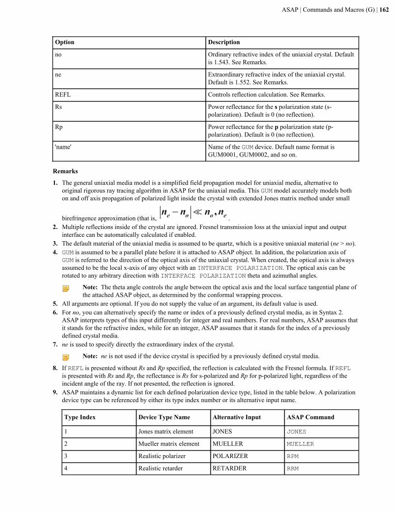
ASAP | Commands and Macros (G) | 162
Option Description
no Ordinary refractive index of the uniaxial crystal. Defaultis 1.543. See Remarks.
ne Extraordinary refractive index of the uniaxial crystal.Default is 1.552. See Remarks.
REFL Controls reflection calculation. See Remarks.
Rs Power reflectance for the s polarization state (s-polarization). Default is 0 (no reflection).
Rp Power reflectance for the p polarization state (p-polarization). Default is 0 (no reflection).
'name' Name of the GUM device. Default name format isGUM0001, GUM0002, and so on.
Remarks
1. The general uniaxial media model is a simplified field propagation model for uniaxial media, alternative tooriginal rigorous ray tracing algorithm in ASAP for the uniaxial media. This GUM model accurately models bothon and off axis propagation of polarized light inside the crystal with extended Jones matrix method under small
birefringence approximation (that is, .2. Multiple reflections inside of the crystal are ignored. Fresnel transmission loss at the uniaxial input and output
interface can be automatically calculated if enabled.3. The default material of the uniaxial media is assumed to be quartz, which is a positive uniaxial material (ne > no).4. GUM is assumed to be a parallel plate before it is attached to ASAP object. In addition, the polarization axis of
GUM is referred to the direction of the optical axis of the uniaxial crystal. When created, the optical axis is alwaysassumed to be the local x-axis of any object with an INTERFACE POLARIZATION. The optical axis can berotated to any arbitrary direction with INTERFACE POLARIZATION theta and azimuthal angles.
Note: The theta angle controls the angle between the optical axis and the local surface tangential plane ofthe attached ASAP object, as determined by the conformal wrapping process.
5. All arguments are optional. If you do not supply the value of an argument, its default value is used.6. For no, you can alternatively specify the name or index of a previously defined crystal media, as in Syntax 2.
ASAP interprets types of this input differently for integer and real numbers. For real numbers, ASAP assumes thatit stands for the refractive index, while for an integer, ASAP assumes that it stands for the index of a previouslydefined crystal media.
7. ne is used to specify directly the extraordinary index of the crystal.
Note: ne is not used if the device crystal is specified by a previously defined crystal media.
8. If REFL is presented without Rs and Rp specified, the reflection is calculated with the Fresnel formula. If REFLis presented with Rs and Rp, the reflectance is Rs for s-polarized and Rp for p-polarized light, regardless of theincident angle of the ray. If not presented, the reflection is ignored.
9. ASAP maintains a dynamic list for each defined polarization device type, listed in the table below. A polarizationdevice type can be referenced by either its type index number or its alternative input name.
Type Index Device Type Name Alternative Input ASAP Command
1 Jones matrix element JONES JONES
2 Mueller matrix element MUELLER MUELLER
3 Realistic polarizer POLARIZER RPM
4 Realistic retarder RETARDER RRM
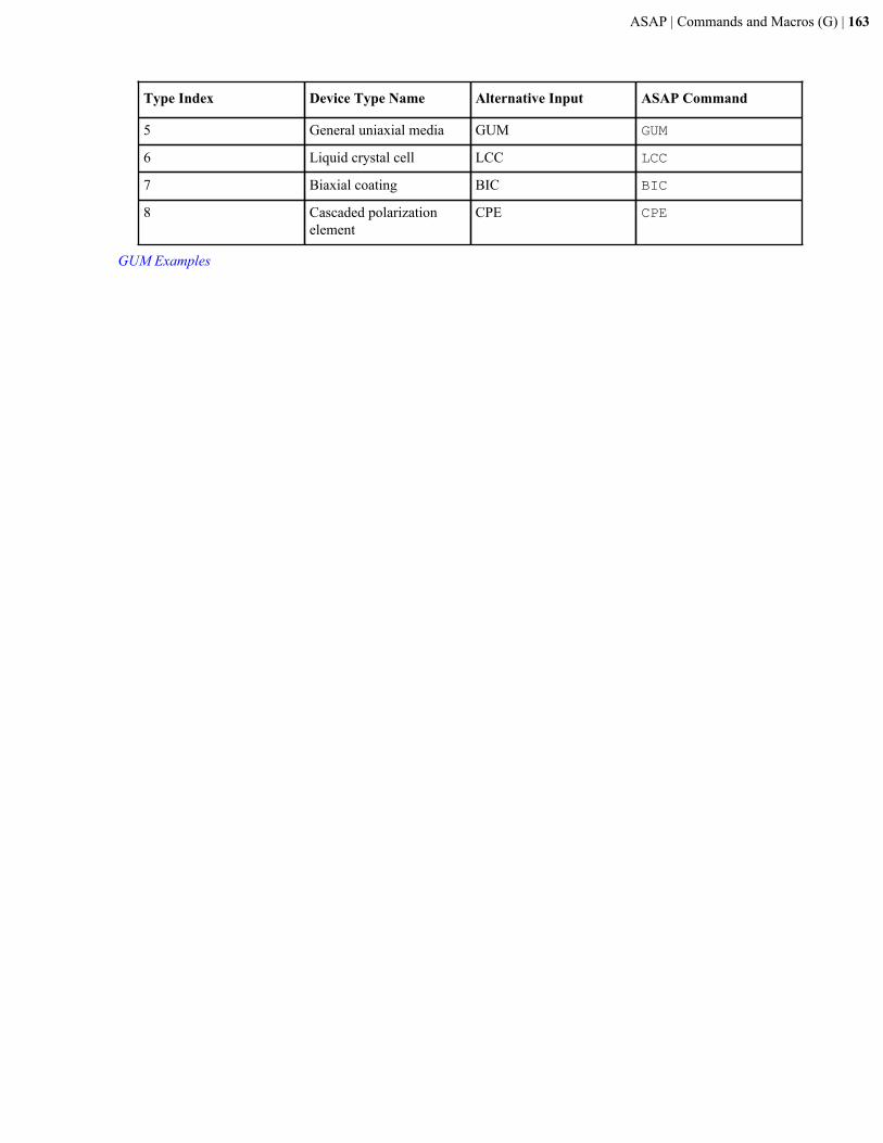
ASAP | Commands and Macros (G) | 163
Type Index Device Type Name Alternative Input ASAP Command
5 General uniaxial media GUM GUM
6 Liquid crystal cell LCC LCC
7 Biaxial coating BIC BIC
8 Cascaded polarizationelement
CPE CPE
GUM Examples
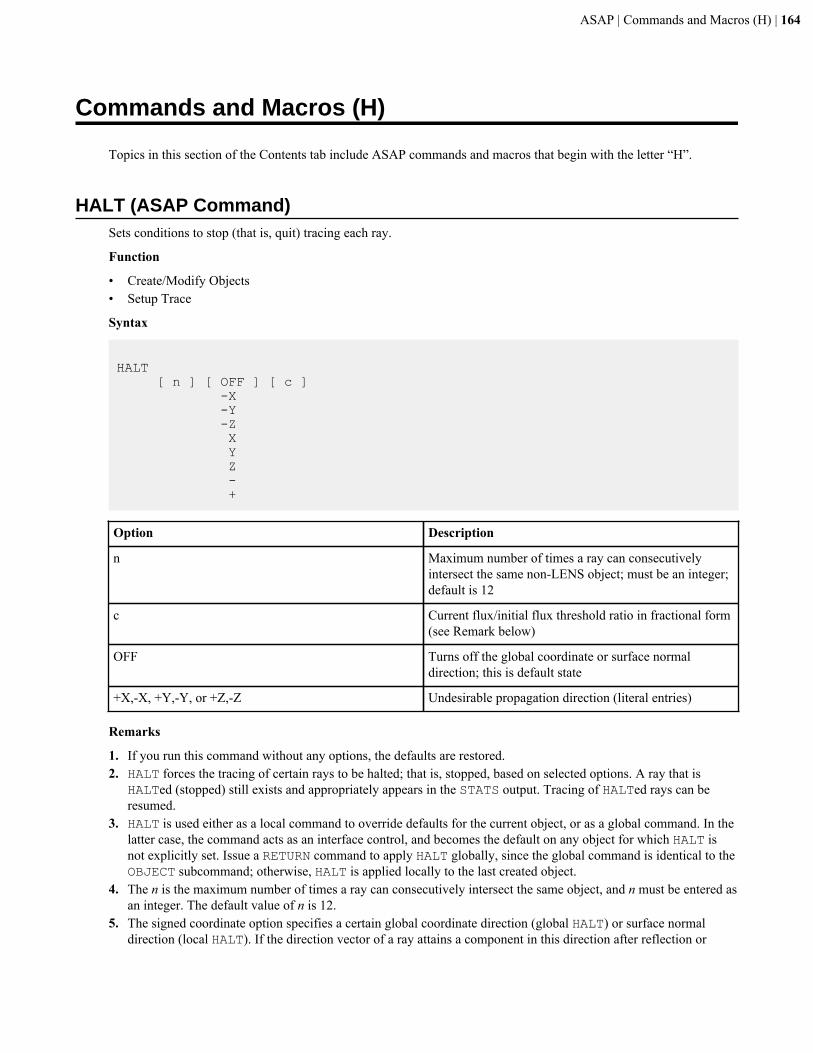
ASAP | Commands and Macros (H) | 164
Commands and Macros (H)
Topics in this section of the Contents tab include ASAP commands and macros that begin with the letter “H”.
HALT (ASAP Command)Sets conditions to stop (that is, quit) tracing each ray.
Function
• Create/Modify Objects• Setup Trace
Syntax
HALT [ n ] [ OFF ] [ c ] -X -Y -Z X Y Z - +
Option Description
n Maximum number of times a ray can consecutivelyintersect the same non-LENS object; must be an integer;default is 12
c Current flux/initial flux threshold ratio in fractional form(see Remark below)
OFF Turns off the global coordinate or surface normaldirection; this is default state
+X,-X, +Y,-Y, or +Z,-Z Undesirable propagation direction (literal entries)
Remarks
1. If you run this command without any options, the defaults are restored.2. HALT forces the tracing of certain rays to be halted; that is, stopped, based on selected options. A ray that is
HALTed (stopped) still exists and appropriately appears in the STATS output. Tracing of HALTed rays can beresumed.
3. HALT is used either as a local command to override defaults for the current object, or as a global command. In thelatter case, the command acts as an interface control, and becomes the default on any object for which HALT isnot explicitly set. Issue a RETURN command to apply HALT globally, since the global command is identical to theOBJECT subcommand; otherwise, HALT is applied locally to the last created object.
4. The n is the maximum number of times a ray can consecutively intersect the same object, and n must be entered asan integer. The default value of n is 12.
5. The signed coordinate option specifies a certain global coordinate direction (global HALT) or surface normaldirection (local HALT). If the direction vector of a ray attains a component in this direction after reflection or
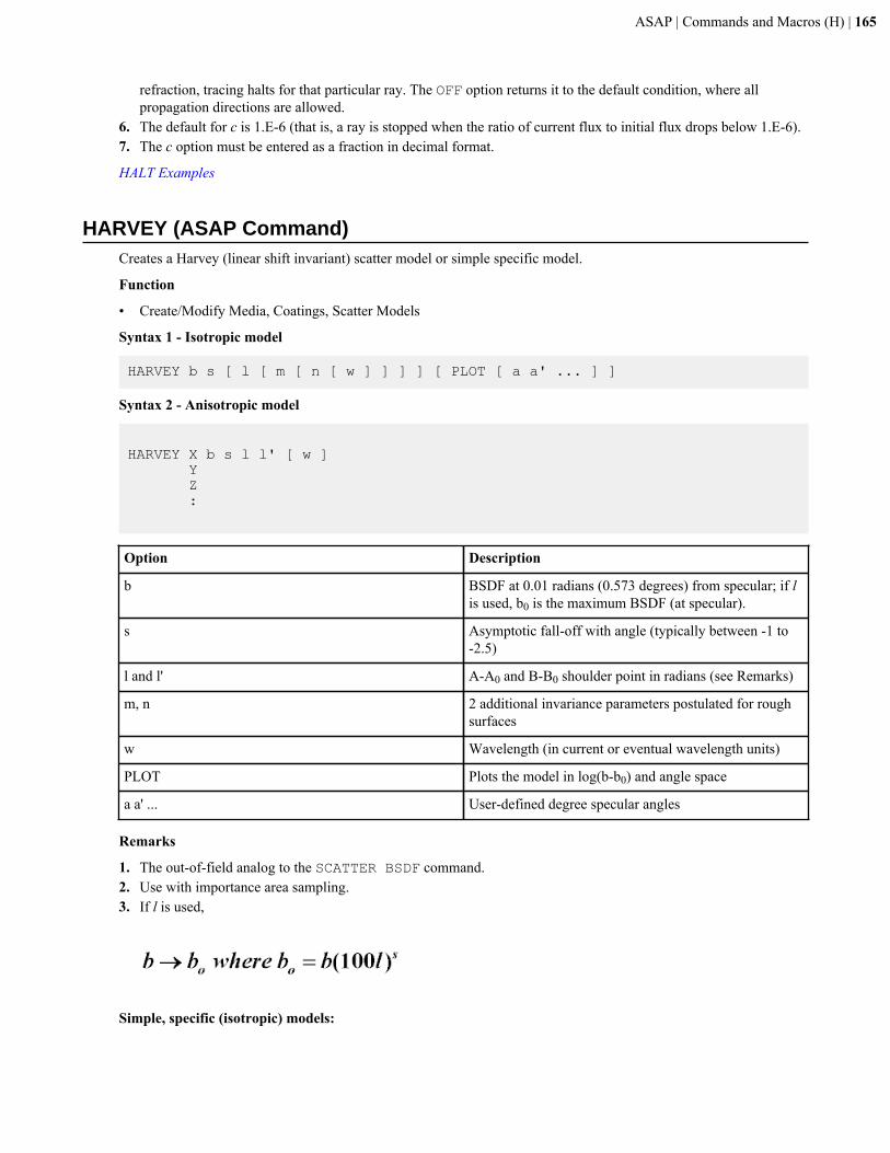
ASAP | Commands and Macros (H) | 165
refraction, tracing halts for that particular ray. The OFF option returns it to the default condition, where allpropagation directions are allowed.
6. The default for c is 1.E-6 (that is, a ray is stopped when the ratio of current flux to initial flux drops below 1.E-6).7. The c option must be entered as a fraction in decimal format.
HALT Examples
HARVEY (ASAP Command)Creates a Harvey (linear shift invariant) scatter model or simple specific model.
Function
• Create/Modify Media, Coatings, Scatter Models
Syntax 1 - Isotropic model
HARVEY b s [ l [ m [ n [ w ] ] ] ] [ PLOT [ a a' ... ] ]
Syntax 2 - Anisotropic model
HARVEY X b s l l' [ w ] Y Z :
Option Description
b BSDF at 0.01 radians (0.573 degrees) from specular; if lis used, b0 is the maximum BSDF (at specular).
s Asymptotic fall-off with angle (typically between -1 to-2.5)
l and l' A-A0 and B-B0 shoulder point in radians (see Remarks)
m, n 2 additional invariance parameters postulated for roughsurfaces
w Wavelength (in current or eventual wavelength units)
PLOT Plots the model in log(b-b0) and angle space
a a' ... User-defined degree specular angles
Remarks
1. The out-of-field analog to the SCATTER BSDF command.2. Use with importance area sampling.3. If l is used,
Simple, specific (isotropic) models:
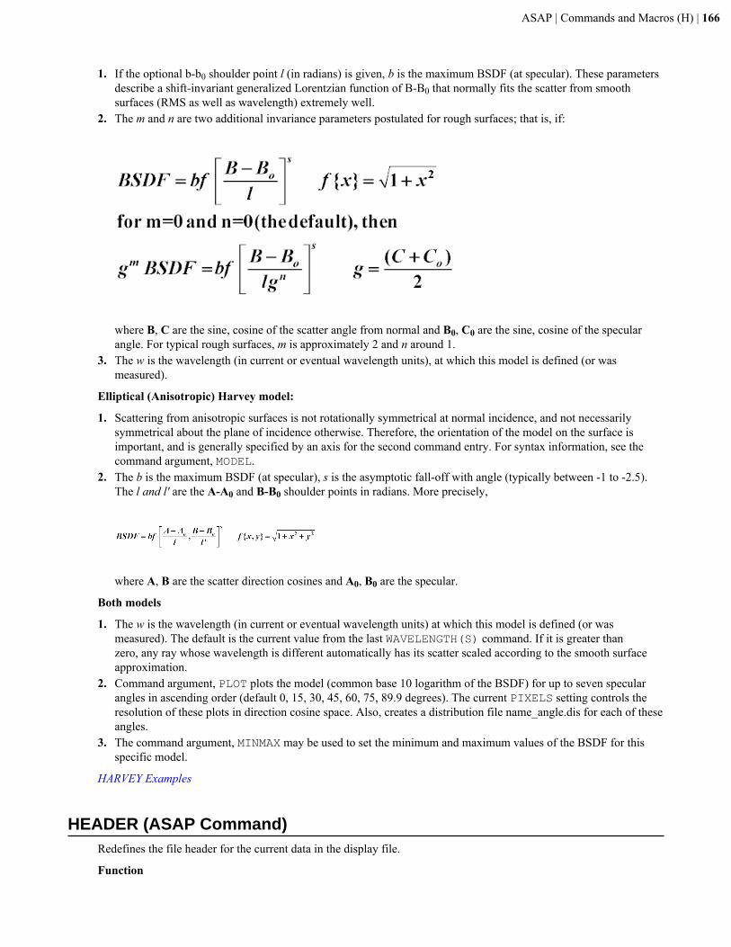
ASAP | Commands and Macros (H) | 166
1. If the optional b-b0 shoulder point l (in radians) is given, b is the maximum BSDF (at specular). These parametersdescribe a shift-invariant generalized Lorentzian function of B-B0 that normally fits the scatter from smoothsurfaces (RMS as well as wavelength) extremely well.
2. The m and n are two additional invariance parameters postulated for rough surfaces; that is, if:
where B, C are the sine, cosine of the scatter angle from normal and B0, C0 are the sine, cosine of the specularangle. For typical rough surfaces, m is approximately 2 and n around 1.
3. The w is the wavelength (in current or eventual wavelength units), at which this model is defined (or wasmeasured).
Elliptical (Anisotropic) Harvey model:
1. Scattering from anisotropic surfaces is not rotationally symmetrical at normal incidence, and not necessarilysymmetrical about the plane of incidence otherwise. Therefore, the orientation of the model on the surface isimportant, and is generally specified by an axis for the second command entry. For syntax information, see thecommand argument, MODEL.
2. The b is the maximum BSDF (at specular), s is the asymptotic fall-off with angle (typically between -1 to -2.5).The l and l' are the A-A0 and B-B0 shoulder points in radians. More precisely,
where A, B are the scatter direction cosines and A0, B0 are the specular.
Both models
1. The w is the wavelength (in current or eventual wavelength units) at which this model is defined (or wasmeasured). The default is the current value from the last WAVELENGTH(S) command. If it is greater thanzero, any ray whose wavelength is different automatically has its scatter scaled according to the smooth surfaceapproximation.
2. Command argument, PLOT plots the model (common base 10 logarithm of the BSDF) for up to seven specularangles in ascending order (default 0, 15, 30, 45, 60, 75, 89.9 degrees). The current PIXELS setting controls theresolution of these plots in direction cosine space. Also, creates a distribution file name_angle.dis for each of theseangles.
3. The command argument, MINMAX may be used to set the minimum and maximum values of the BSDF for thisspecific model.
HARVEY Examples
HEADER (ASAP Command)Redefines the file header for the current data in the display file.
Function
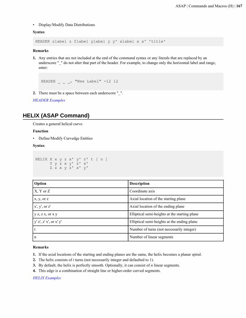
ASAP | Commands and Macros (H) | 167
• Display/Modify Data Distributions
Syntax
HEADER zlabel z flabel ylabel y y' xlabel x x' 'title'
Remarks
1. Any entries that are not included at the end of the command syntax or any literals that are replaced by anunderscore "_" do not alter that part of the header. For example, to change only the horizontal label and range,enter:
HEADER _ _ _, "New Label" -12 12
2. There must be a space between each underscore "_".
HEADER Examples
HELIX (ASAP Command)Creates a general helical curve.
Function
• Define/Modify Curvedge Entities
Syntax
HELIX X x y z x' y' z' t [ n ] Y y z x y' z' x' Z z x y z' x' y'
Option Description
X, Y or Z Coordinate axis
x, y, or z Axial location of the starting plane
x', y', or z' Axial location of the ending plane
y z, z x, or x y Elliptical semi-heights at the starting plane
y' z', z' x', or x' y' Elliptical semi-heights at the ending plane
t Number of turns (not necessarily integer)
n Number of linear segments
Remarks
1. If the axial locations of the starting and ending planes are the same, the helix becomes a planar spiral.2. The helix consists of t turns (not necessarily integer and defaulted to 1).3. By default, the helix is perfectly smooth. Optionally, it can consist of n linear segments.4. This edge is a combination of straight line or higher-order curved segments.
HELIX Examples
ASAP | Commands and Macros (H) | 168
$HELP (ASAP Macro)Displays information on all or one command or a listing of the MACROS in the current library.
Syntax
$HELP [ command ]
Remarks
1. The content that is displayed by $HELP is archival. Please see ASAP Help for current information on anycommand or macro. ASAP Help is acccessible by highlighting a command name in an INR file and clickingF1, by clicking Content on the Help menu in ASAP, or in the bin folder of your ASAP installation area(ASAP_Help.chm).
2. $HELP displays a popup window that lists many ASAP commands. Upon selecting a command on the list, thecontent is displayed in the output window. For example, OBJECTS; $HELP displays a popup window that listsonly object modifier commands; $IO LIB UTIL lists the utility .lib file; and $HELP MACROS opens a windowthat lists all macros in the macros .lib file.
3. If no entry is given, an abbreviated list of all commands is displayed.4. If only one command (up to two literals) is specified, a complete one or two paragraph explanation of the
command is shown.5. The &HELP form displays only the format of the command with no accompanying text.
$HELP Examples
HISTOGRAM (ASAP Command)Displays a plot of the number of data values.
Function
• Display/Modify Data Distributions
Syntax
HISTOGRAM [ n ] [ w ] [ NORMALIZED ] PROBABILITY
Options Description
n Number of intervals
w Relative width of the plot bars
NORMALIZED Sets the peak value to unity
PROBABILITY Scales the data values (see Remarks)
Remarks
1. Displays a plot of the number of data values within n intervals (equally spaced between the minimum andmaximum values). The default for n is 21.
2. The w option controls the relative width of the plotted bars (see GRAPH DISCRETE). The default for w is 0.4.The range for w is greater than 0 and less than 0.5.
3. The plot can be optionally NORMALIZED to a peak value of one.4. The PROBABILITY option scales the data values so that the area under the curve is unity, consistent with the
definition of a probability density function.
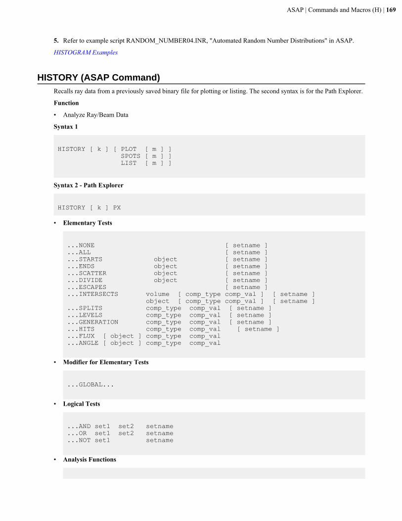
ASAP | Commands and Macros (H) | 169
5. Refer to example script RANDOM_NUMBER04.INR, "Automated Random Number Distributions" in ASAP.
HISTOGRAM Examples
HISTORY (ASAP Command)Recalls ray data from a previously saved binary file for plotting or listing. The second syntax is for the Path Explorer.
Function
• Analyze Ray/Beam Data
Syntax 1
HISTORY [ k ] [ PLOT [ m ] ] SPOTS [ m ] ] LIST [ m ] ]
Syntax 2 - Path Explorer
HISTORY [ k ] PX
• Elementary Tests
...NONE [ setname ]
...ALL [ setname ]
...STARTS object [ setname ]
...ENDS object [ setname ]
...SCATTER object [ setname ]
...DIVIDE object [ setname ]
...ESCAPES [ setname ]
...INTERSECTS volume [ comp_type comp_val ] [ setname ] object [ comp_type comp_val ] [ setname ]...SPLITS comp_type comp_val [ setname ]...LEVELS comp_type comp_val [ setname ]...GENERATION comp_type comp_val [ setname ]...HITS comp_type comp_val [ setname ]...FLUX [ object ] comp_type comp_val...ANGLE [ object ] comp_type comp_val
• Modifier for Elementary Tests
...GLOBAL...
• Logical Tests
...AND set1 set2 setname
...OR set1 set2 setname
...NOT set1 setname
• Analysis Functions

ASAP | Commands and Macros (H) | 170
...LIST [ setname ] [ m ]
...PLOT [ setname ] [ m ]
...SPOTS [ setname ] [ m ]
...WINDOW...
...REFRESH
...SUMMARY [ setname ]
• Session Management
...STORE setname
...RECALL [ setname ]
...RETURN
Option Description
k SAVE file number from the last TRACE command
LIST LIST the trajectories in the selected path-set
PLOT PLOT paths graphically for the selected path-set
SPOTS Display a spots diagram for the selected path-set
m Stride (default 1) with which to choose paths output byPLOT, SPOTS or LIST; that is, every mth ray.
WINDOW Set window parameters for plotting paths; see mainWINDOW command
REFRESH Refresh the 3D graphics file for plotting paths
SUMMARY Report statistics on the selected path-set
GLOBAL Modifier that can appear only at the end of anyElementary Test and specifies that the test applies to theentire ray history file (not the ACTIVE path-set)
NONE Creates a path-set containing no paths and makes this theactive set
ALL Creates a path-set containing all paths and makes this theactive set
STARTS Creates a path-set containing all paths in the active setstarting on a specified object
ENDS Creates a path-set containing all paths in the active setending on a specified object
SCATTER Creates a path-set containing all paths in the active setscattering from the specified object
DIVIDE Creates a path-set containing all paths in the active setsplitting from the specified object
ESCAPES Creates a path-set containing all paths in the active setthat escaped; that is, missed rays.
INTERSECTS Creates a path-set containing all paths in the active set,including a specified number of, or upper bound or lowerbound on, the number of intersections with a specified
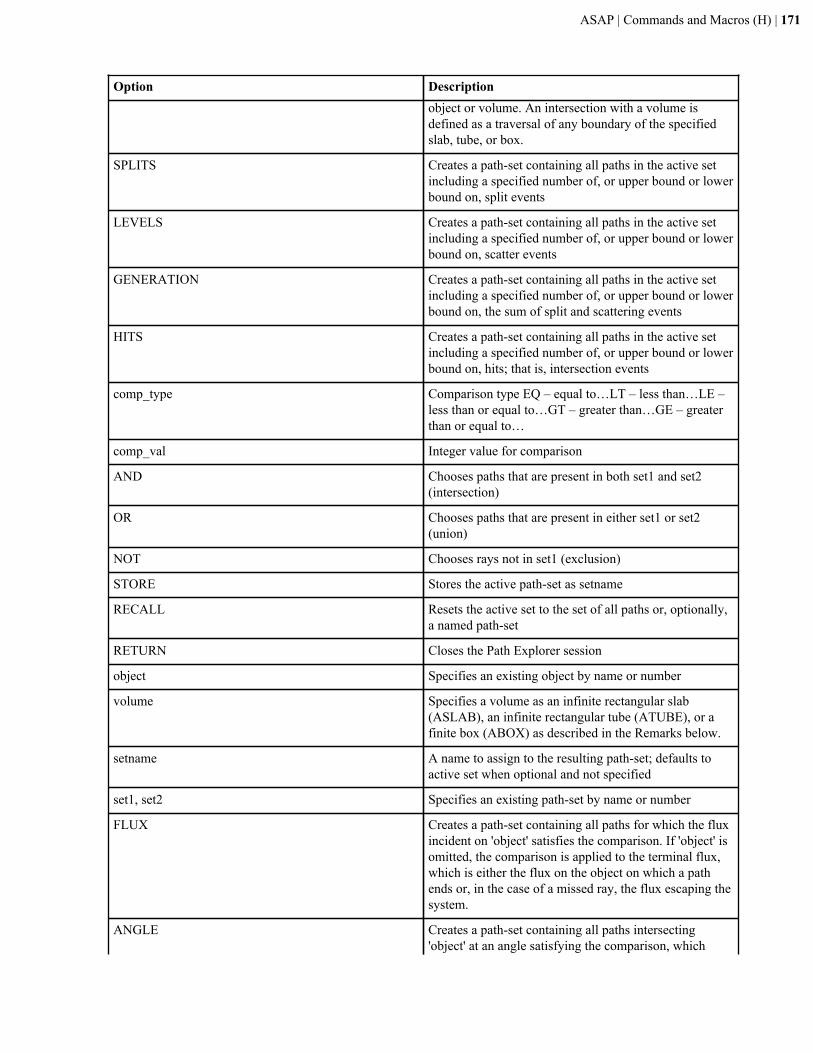
ASAP | Commands and Macros (H) | 171
Option Descriptionobject or volume. An intersection with a volume isdefined as a traversal of any boundary of the specifiedslab, tube, or box.
SPLITS Creates a path-set containing all paths in the active setincluding a specified number of, or upper bound or lowerbound on, split events
LEVELS Creates a path-set containing all paths in the active setincluding a specified number of, or upper bound or lowerbound on, scatter events
GENERATION Creates a path-set containing all paths in the active setincluding a specified number of, or upper bound or lowerbound on, the sum of split and scattering events
HITS Creates a path-set containing all paths in the active setincluding a specified number of, or upper bound or lowerbound on, hits; that is, intersection events
comp_type Comparison type EQ – equal to…LT – less than…LE –less than or equal to…GT – greater than…GE – greaterthan or equal to…
comp_val Integer value for comparison
AND Chooses paths that are present in both set1 and set2(intersection)
OR Chooses paths that are present in either set1 or set2(union)
NOT Chooses rays not in set1 (exclusion)
STORE Stores the active path-set as setname
RECALL Resets the active set to the set of all paths or, optionally,a named path-set
RETURN Closes the Path Explorer session
object Specifies an existing object by name or number
volume Specifies a volume as an infinite rectangular slab(ASLAB), an infinite rectangular tube (ATUBE), or afinite box (ABOX) as described in the Remarks below.
setname A name to assign to the resulting path-set; defaults toactive set when optional and not specified
set1, set2 Specifies an existing path-set by name or number
FLUX Creates a path-set containing all paths for which the fluxincident on 'object' satisfies the comparison. If 'object' isomitted, the comparison is applied to the terminal flux,which is either the flux on the object on which a pathends or, in the case of a missed ray, the flux escaping thesystem.
ANGLE Creates a path-set containing all paths intersecting'object' at an angle satisfying the comparison, which
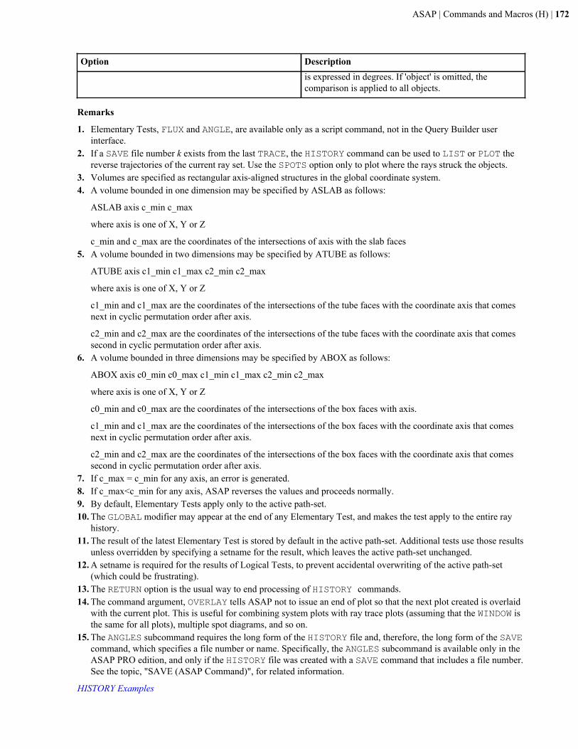
ASAP | Commands and Macros (H) | 172
Option Descriptionis expressed in degrees. If 'object' is omitted, thecomparison is applied to all objects.
Remarks
1. Elementary Tests, FLUX and ANGLE, are available only as a script command, not in the Query Builder userinterface.
2. If a SAVE file number k exists from the last TRACE, the HISTORY command can be used to LIST or PLOT thereverse trajectories of the current ray set. Use the SPOTS option only to plot where the rays struck the objects.
3. Volumes are specified as rectangular axis-aligned structures in the global coordinate system.4. A volume bounded in one dimension may be specified by ASLAB as follows:
ASLAB axis c_min c_max
where axis is one of X, Y or Z
c_min and c_max are the coordinates of the intersections of axis with the slab faces5. A volume bounded in two dimensions may be specified by ATUBE as follows:
ATUBE axis c1_min c1_max c2_min c2_max
where axis is one of X, Y or Z
c1_min and c1_max are the coordinates of the intersections of the tube faces with the coordinate axis that comesnext in cyclic permutation order after axis.
c2_min and c2_max are the coordinates of the intersections of the tube faces with the coordinate axis that comessecond in cyclic permutation order after axis.
6. A volume bounded in three dimensions may be specified by ABOX as follows:
ABOX axis c0_min c0_max c1_min c1_max c2_min c2_max
where axis is one of X, Y or Z
c0_min and c0_max are the coordinates of the intersections of the box faces with axis.
c1_min and c1_max are the coordinates of the intersections of the box faces with the coordinate axis that comesnext in cyclic permutation order after axis.
c2_min and c2_max are the coordinates of the intersections of the box faces with the coordinate axis that comessecond in cyclic permutation order after axis.
7. If c_max = c_min for any axis, an error is generated.8. If c_max<c_min for any axis, ASAP reverses the values and proceeds normally.9. By default, Elementary Tests apply only to the active path-set.10. The GLOBAL modifier may appear at the end of any Elementary Test, and makes the test apply to the entire ray
history.11. The result of the latest Elementary Test is stored by default in the active path-set. Additional tests use those results
unless overridden by specifying a setname for the result, which leaves the active path-set unchanged.12. A setname is required for the results of Logical Tests, to prevent accidental overwriting of the active path-set
(which could be frustrating).13. The RETURN option is the usual way to end processing of HISTORY commands.14. The command argument, OVERLAY tells ASAP not to issue an end of plot so that the next plot created is overlaid
with the current plot. This is useful for combining system plots with ray trace plots (assuming that the WINDOW isthe same for all plots), multiple spot diagrams, and so on.
15. The ANGLES subcommand requires the long form of the HISTORY file and, therefore, the long form of the SAVEcommand, which specifies a file number or name. Specifically, the ANGLES subcommand is available only in theASAP PRO edition, and only if the HISTORY file was created with a SAVE command that includes a file number.See the topic, "SAVE (ASAP Command)", for related information.
HISTORY Examples
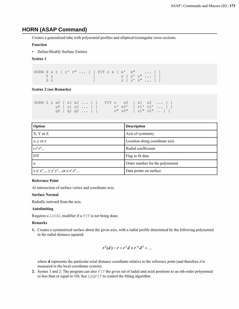
ASAP | Commands and Macros (H) | 173
HORN (ASAP Command)Creates a generalized tube with polynomial profiles and elliptical/rectangular cross-sections.
Function
• Define/Modify Surfunc Entities
Syntax 1
HORN X x r [ r' r" ... ] [ FIT n x [ x' x" ... ] ] Y y [ y [ y' y" ... ] ] Z z [ z [ z' z" ... ] ]
Syntax 2 (see Remarks)
HORN Z z x0 [ x1 x2 ... ] [ FIT n z0 [ z1 z2 ... ] ] y0 [ y1 y2 ... ] [ n' z0' [ z1' z2' ... ] ] q0 [ q1 q2 ... ] [ n" z0" [ z1" z2" .. ] ]
Option Description
X, Y or Z Axis of symmetry
x, y or z Location along coordinate axis
r r' r"... Radial coefficients
FIT Flag to fit data
n Order number for the polynomial
x x' x"..., y y' y"...,or z z' z"... Data points on surface
Reference Point
At intersection of surface vertex and coordinate axis.
Surface Normal
Radially outward from the axis.
Autolimiting
Requires a LOCAL modifier if a FIT is not being done.
Remarks
1. Creates a symmetrical surface about the given axis, with a radial profile determined by the following polynomialin the radial distance squared:
where d represents the particular axial distance coordinate relative to the reference point (and therefore d ismeasured in the local coordinate system).
2. Syntax 1 and 2: The program can also FIT the given set of radial and axial positions to an nth-order polynomial(n less than or equal to 10). See LSQFIT to control the fitting algorithm.
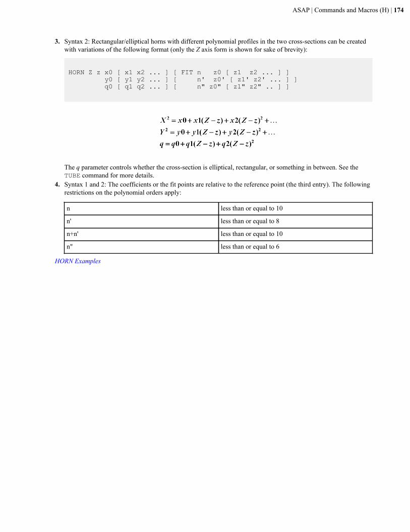
ASAP | Commands and Macros (H) | 174
3. Syntax 2: Rectangular/elliptical horns with different polynomial profiles in the two cross-sections can be createdwith variations of the following format (only the Z axis form is shown for sake of brevity):
HORN Z z x0 [ x1 x2 ... ] [ FIT n z0 [ z1 z2 ... ] ] y0 [ y1 y2 ... ] [ n' z0' [ z1' z2' ... ] ] q0 [ q1 q2 ... ] [ n" z0" [ z1" z2" .. ] ]
The q parameter controls whether the cross-section is elliptical, rectangular, or something in between. See theTUBE command for more details.
4. Syntax 1 and 2: The coefficients or the fit points are relative to the reference point (the third entry). The followingrestrictions on the polynomial orders apply:
n less than or equal to 10
n' less than or equal to 8
n+n' less than or equal to 10
n" less than or equal to 6
HORN Examples
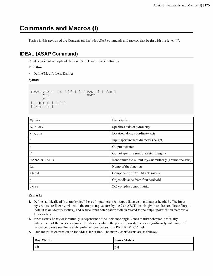
ASAP | Commands and Macros (I) | 175
Commands and Macros (I)
Topics in this section of the Contents tab include ASAP commands and macros that begin with the letter “I”.
IDEAL (ASAP Command)Creates an idealized optical element (ABCD and Jones matrices).
Function
• Define/Modify Lens Entities
Syntax
IDEAL X x h [ t [ h' ] ] [ RANA ] [ fcn ] Y y RANB Z z[ a b c d [ o ] ][ p q r s ]
Option Description
X, Y, or Z Specifies axis of symmetry
x, y, or z Location along coordinate axis
h Input aperture semidiameter (height)
t Output distance
h' Output aperture semidiameter (height)
RANA or RANB Randomize the output rays azimuthally (around the axis)
fcn Name of the function
a b c d Components of 2x2 ABCD matrix
o Object distance from first conicoid
p q r s 2x2 complex Jones matrix
Remarks
1. Defines an idealized (but unphysical) lens of input height h, output distance t, and output height h'. The inputray vectors are linearly related to the output ray vectors by the 2x2 ABCD matrix given on the next line of input(default is an identity matrix), and whose input polarization state is related to the output polarization state via aJones matrix.
2. Jones matrix behavior is virtually independent of the incidence angle. Jones matrix behavior is virtuallyindependent of the incidence angle. For devices where the polarization state varies significantly with angle ofincidence, please see the realistic polarizer devices such as RRP, RPM, CPE, etc.
3. Each matrix is entered on an individual input line. The matrix coefficients are as follows:
Ray Matrix Jones Matrix
a b p q
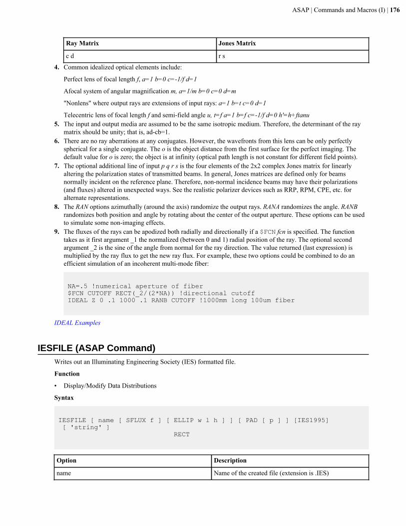
ASAP | Commands and Macros (I) | 176
Ray Matrix Jones Matrix
c d r s
4. Common idealized optical elements include:
Perfect lens of focal length f, a=1 b=0 c=-1/f d=1
Afocal system of angular magnification m, a=1/m b=0 c=0 d=m
"Nonlens" where output rays are extensions of input rays: a=1 b=t c=0 d=1
Telecentric lens of focal length f and semi-field angle u, t=f a=1 b=f c=-1/f d=0 h'=h+ftanu5. The input and output media are assumed to be the same isotropic medium. Therefore, the determinant of the ray
matrix should be unity; that is, ad-cb=1.6. There are no ray aberrations at any conjugates. However, the wavefronts from this lens can be only perfectly
spherical for a single conjugate. The o is the object distance from the first surface for the perfect imaging. Thedefault value for o is zero; the object is at infinity (optical path length is not constant for different field points).
7. The optional additional line of input p q r s is the four elements of the 2x2 complex Jones matrix for linearlyaltering the polarization states of transmitted beams. In general, Jones matrices are defined only for beamsnormally incident on the reference plane. Therefore, non-normal incidence beams may have their polarizations(and fluxes) altered in unexpected ways. See the realistic polarizer devices such as RRP, RPM, CPE, etc. foralternate representations.
8. The RAN options azimuthally (around the axis) randomize the output rays. RANA randomizes the angle. RANBrandomizes both position and angle by rotating about the center of the output aperture. These options can be usedto simulate some non-imaging effects.
9. The fluxes of the rays can be apodized both radially and directionally if a $FCN fcn is specified. The functiontakes as it first argument _1 the normalized (between 0 and 1) radial position of the ray. The optional secondargument _2 is the sine of the angle from normal for the ray direction. The value returned (last expression) ismultiplied by the ray flux to get the new ray flux. For example, these two options could be combined to do anefficient simulation of an incoherent multi-mode fiber:
NA=.5 !numerical aperture of fiber$FCN CUTOFF RECT(_2/(2*NA)) !directional cutoffIDEAL Z 0 .1 1000 .1 RANB CUTOFF !1000mm long 100um fiber
IDEAL Examples
IESFILE (ASAP Command)Writes out an Illuminating Engineering Society (IES) formatted file.
Function
• Display/Modify Data Distributions
Syntax
IESFILE [ name [ SFLUX f ] [ ELLIP w l h ] ] [ PAD [ p ] ] [IES1995] [ 'string' ] RECT
Option Description
name Name of the created file (extension is .IES)
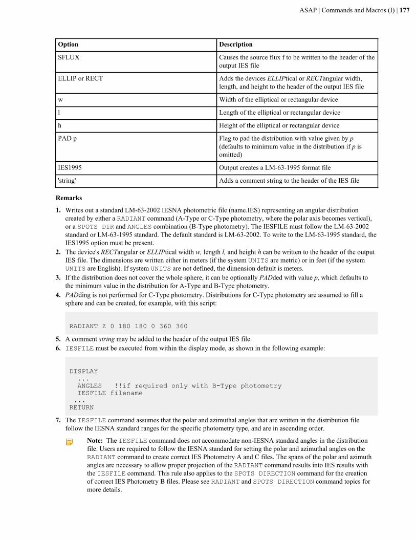
ASAP | Commands and Macros (I) | 177
Option Description
SFLUX Causes the source flux f to be written to the header of theoutput IES file
ELLIP or RECT Adds the devices ELLIPtical or RECTangular width,length, and height to the header of the output IES file
w Width of the elliptical or rectangular device
l Length of the elliptical or rectangular device
h Height of the elliptical or rectangular device
PAD p Flag to pad the distribution with value given by p(defaults to minimum value in the distribution if p isomitted)
IES1995 Output creates a LM-63-1995 format file
'string' Adds a comment string to the header of the IES file
Remarks
1. Writes out a standard LM-63-2002 IESNA photometric file (name.IES) representing an angular distributioncreated by either a RADIANT command (A-Type or C-Type photometry, where the polar axis becomes vertical),or a SPOTS DIR and ANGLES combination (B-Type photometry). The IESFILE must follow the LM-63-2002standard or LM-63-1995 standard. The default standard is LM-63-2002. To write to the LM-63-1995 standard, theIES1995 option must be present.
2. The device's RECTangular or ELLIPtical width w, length l, and height h can be written to the header of the outputIES file. The dimensions are written either in meters (if the system UNITS are metric) or in feet (if the systemUNITS are English). If system UNITS are not defined, the dimension default is meters.
3. If the distribution does not cover the whole sphere, it can be optionally PADded with value p, which defaults tothe minimum value in the distribution for A-Type and B-Type photometry.
4. PADding is not performed for C-Type photometry. Distributions for C-Type photometry are assumed to fill asphere and can be created, for example, with this script:
RADIANT Z 0 180 180 0 360 360
5. A comment string may be added to the header of the output IES file.6. IESFILE must be executed from within the display mode, as shown in the following example:
DISPLAY ... ANGLES !!if required only with B-Type photometry IESFILE filename ...RETURN
7. The IESFILE command assumes that the polar and azimuthal angles that are written in the distribution filefollow the IESNA standard ranges for the specific photometry type, and are in ascending order.
Note: The IESFILE command does not accommodate non-IESNA standard angles in the distributionfile. Users are required to follow the IESNA standard for setting the polar and azimuthal angles on theRADIANT command to create correct IES Photometry A and C files. The spans of the polar and azimuthangles are necessary to allow proper projection of the RADIANT command results into IES results withthe IESFILE command. This rule also applies to the SPOTS DIRECTION command for the creationof correct IES Photometry B files. Please see RADIANT and SPOTS DIRECTION command topics formore details.
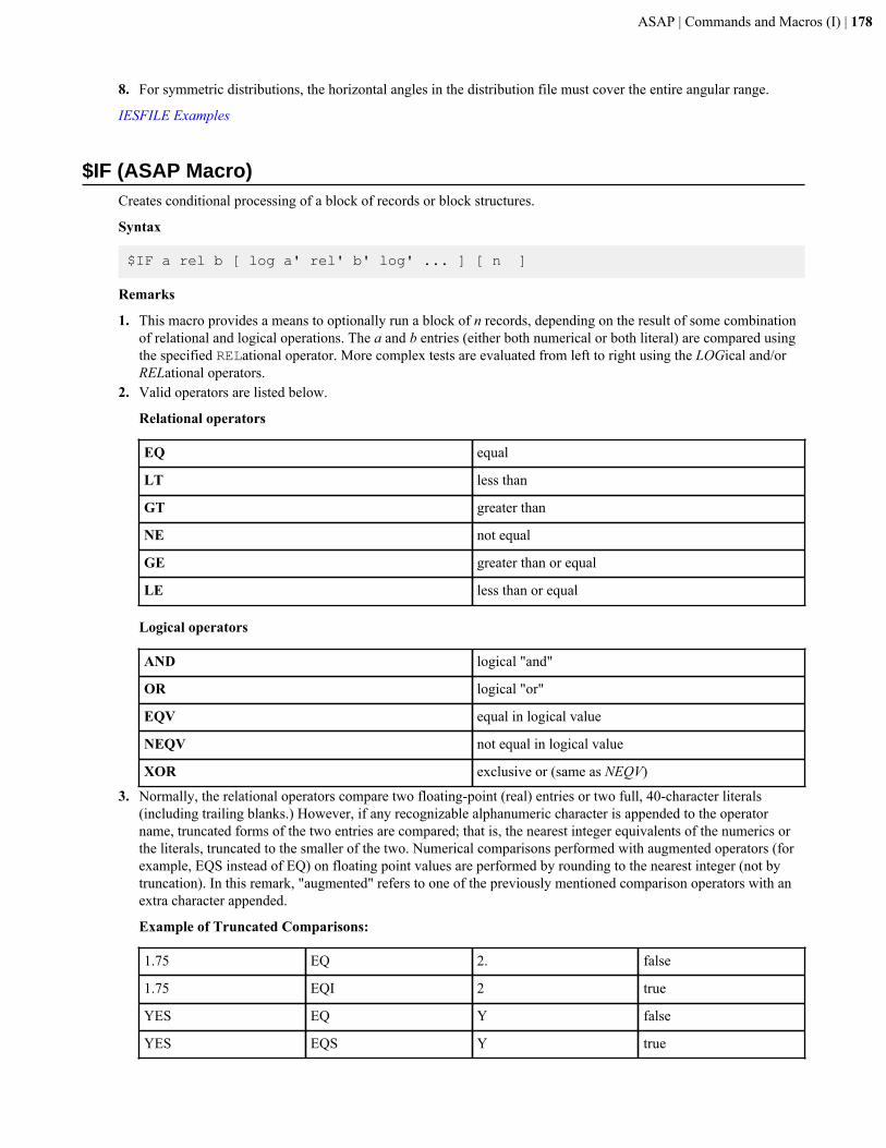
ASAP | Commands and Macros (I) | 178
8. For symmetric distributions, the horizontal angles in the distribution file must cover the entire angular range.
IESFILE Examples
$IF (ASAP Macro)Creates conditional processing of a block of records or block structures.
Syntax
$IF a rel b [ log a' rel' b' log' ... ] [ n ]
Remarks
1. This macro provides a means to optionally run a block of n records, depending on the result of some combinationof relational and logical operations. The a and b entries (either both numerical or both literal) are compared usingthe specified RELational operator. More complex tests are evaluated from left to right using the LOGical and/orRELational operators.
2. Valid operators are listed below.
Relational operators
EQ equal
LT less than
GT greater than
NE not equal
GE greater than or equal
LE less than or equal
Logical operators
AND logical "and"
OR logical "or"
EQV equal in logical value
NEQV not equal in logical value
XOR exclusive or (same as NEQV)
3. Normally, the relational operators compare two floating-point (real) entries or two full, 40-character literals(including trailing blanks.) However, if any recognizable alphanumeric character is appended to the operatorname, truncated forms of the two entries are compared; that is, the nearest integer equivalents of the numerics orthe literals, truncated to the smaller of the two. Numerical comparisons performed with augmented operators (forexample, EQS instead of EQ) on floating point values are performed by rounding to the nearest integer (not bytruncation). In this remark, "augmented" refers to one of the previously mentioned comparison operators with anextra character appended.
Example of Truncated Comparisons:
1.75 EQ 2. false
1.75 EQI 2 true
YES EQ Y false
YES EQS Y true
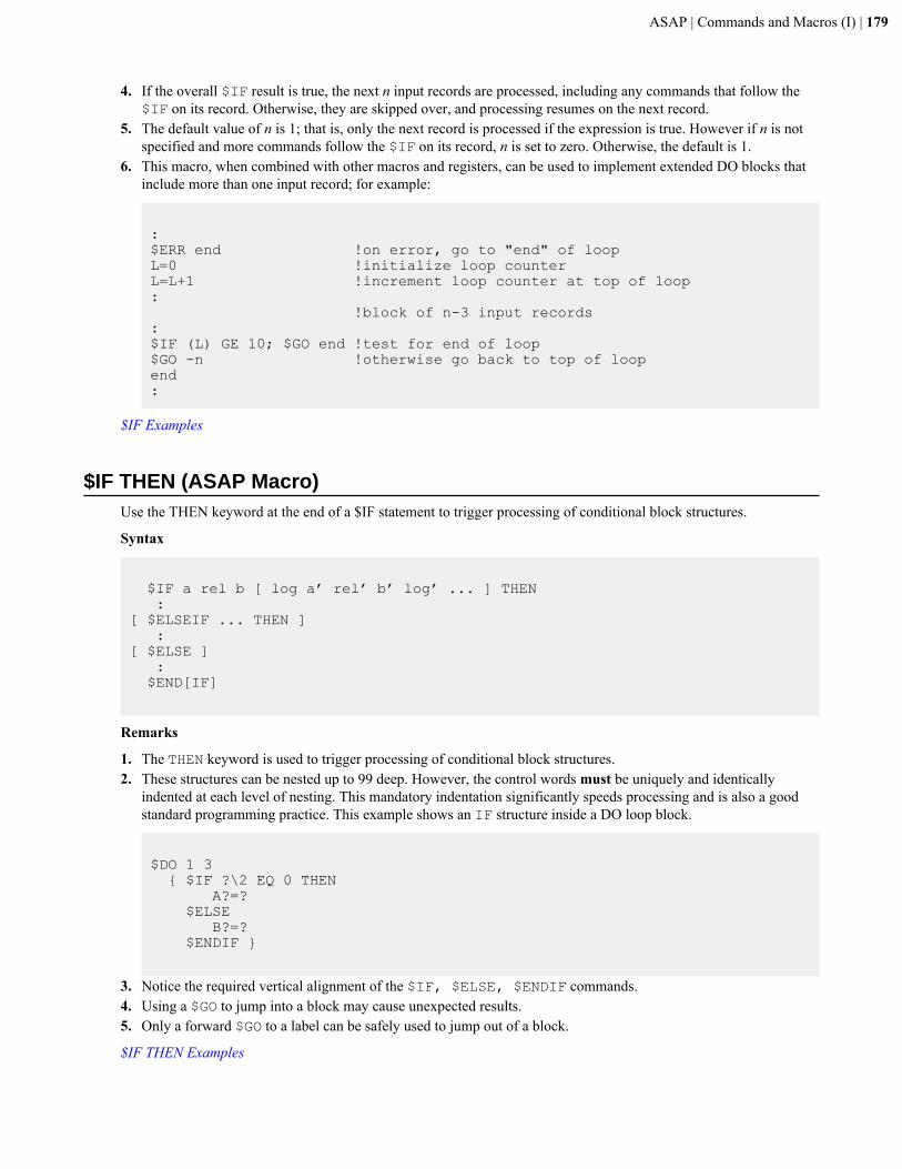
ASAP | Commands and Macros (I) | 179
4. If the overall $IF result is true, the next n input records are processed, including any commands that follow the$IF on its record. Otherwise, they are skipped over, and processing resumes on the next record.
5. The default value of n is 1; that is, only the next record is processed if the expression is true. However if n is notspecified and more commands follow the $IF on its record, n is set to zero. Otherwise, the default is 1.
6. This macro, when combined with other macros and registers, can be used to implement extended DO blocks thatinclude more than one input record; for example:
:$ERR end !on error, go to "end" of loopL=0 !initialize loop counterL=L+1 !increment loop counter at top of loop: !block of n-3 input records:$IF (L) GE 10; $GO end !test for end of loop$GO -n !otherwise go back to top of loopend:
$IF Examples
$IF THEN (ASAP Macro)Use the THEN keyword at the end of a $IF statement to trigger processing of conditional block structures.
Syntax
$IF a rel b [ log a’ rel’ b’ log’ ... ] THEN :[ $ELSEIF ... THEN ] :[ $ELSE ] : $END[IF]
Remarks
1. The THEN keyword is used to trigger processing of conditional block structures.2. These structures can be nested up to 99 deep. However, the control words must be uniquely and identically
indented at each level of nesting. This mandatory indentation significantly speeds processing and is also a goodstandard programming practice. This example shows an IF structure inside a DO loop block.
$DO 1 3 { $IF ?\2 EQ 0 THEN A?=? $ELSE B?=? $ENDIF }
3. Notice the required vertical alignment of the $IF, $ELSE, $ENDIF commands.4. Using a $GO to jump into a block may cause unexpected results.5. Only a forward $GO to a label can be safely used to jump out of a block.
$IF THEN Examples
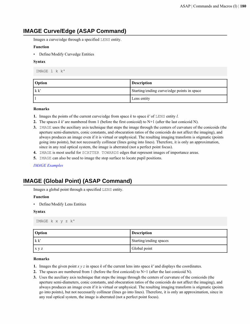
ASAP | Commands and Macros (I) | 180
IMAGE Curve/Edge (ASAP Command)Images a curve/edge through a specified LENS entity.
Function
• Define/Modify Curvedge Entities
Syntax
IMAGE l k k'
Option Description
k k' Starting/ending curve/edge points in space
l Lens entity
Remarks
1. Images the points of the current curve/edge from space k to space k' of LENS entity l.2. The spaces k k' are numbered from 1 (before the first conicoid) to N+1 (after the last conicoid N).3. IMAGE uses the auxiliary axis technique that steps the image through the centers of curvature of the conicoids (the
aperture semi-diameters, conic constants, and obscuration ratios of the conicoids do not affect the imaging), andalways produces an image even if it is virtual or unphysical. The resulting imaging transform is stigmatic (pointsgoing into points), but not necessarily collinear (lines going into lines). Therefore, it is only an approximation,since in any real optical system, the image is aberrated (not a perfect point focus).
4. IMAGE is most useful for SCATTER TOWARDS edges that represent images of importance areas.5. IMAGE can also be used to image the stop surface to locate pupil positions.
IMAGE Examples
IMAGE (Global Point) (ASAP Command)Images a global point through a specified LENS entity.
Function
• Define/Modify Lens Entities
Syntax
IMAGE k x y z k'
Option Description
k k' Starting/ending spaces
x y z Global point
Remarks
1. Images the given point x y z in space k of the current lens into space k' and displays the coordinates.2. The spaces are numbered from 1 (before the first conicoid) to N+1 (after the last conicoid N).3. Uses the auxiliary axis technique that steps the image through the centers of curvature of the conicoids (the
aperture semi-diameters, conic constants, and obscuration ratios of the conicoids do not affect the imaging), andalways produces an image even if it is virtual or unphysical. The resulting imaging transform is stigmatic (pointsgo into points), but not necessarily collinear (lines go into lines). Therefore, it is only an approximation, since inany real optical system, the image is aberrated (not a perfect point focus).
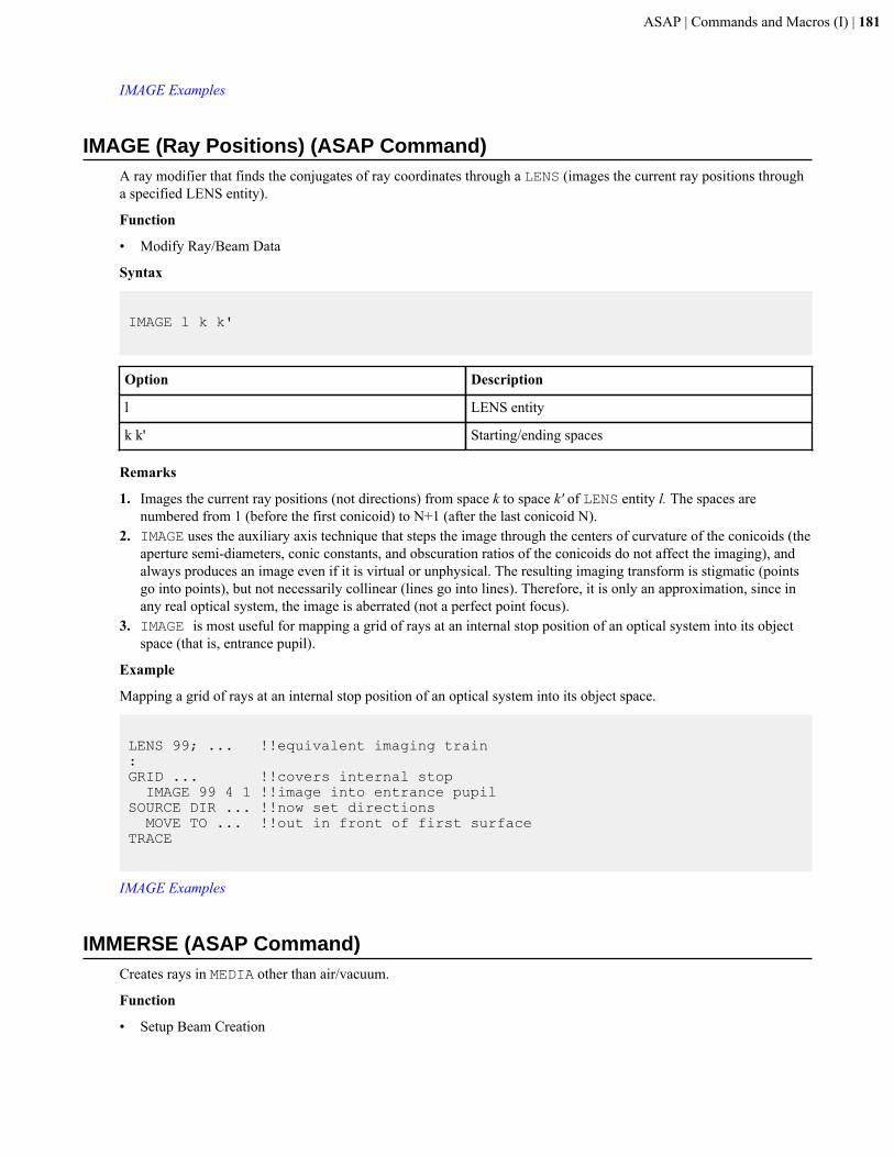
ASAP | Commands and Macros (I) | 181
IMAGE Examples
IMAGE (Ray Positions) (ASAP Command)A ray modifier that finds the conjugates of ray coordinates through a LENS (images the current ray positions througha specified LENS entity).
Function
• Modify Ray/Beam Data
Syntax
IMAGE l k k'
Option Description
l LENS entity
k k' Starting/ending spaces
Remarks
1. Images the current ray positions (not directions) from space k to space k' of LENS entity l. The spaces arenumbered from 1 (before the first conicoid) to N+1 (after the last conicoid N).
2. IMAGE uses the auxiliary axis technique that steps the image through the centers of curvature of the conicoids (theaperture semi-diameters, conic constants, and obscuration ratios of the conicoids do not affect the imaging), andalways produces an image even if it is virtual or unphysical. The resulting imaging transform is stigmatic (pointsgo into points), but not necessarily collinear (lines go into lines). Therefore, it is only an approximation, since inany real optical system, the image is aberrated (not a perfect point focus).
3. IMAGE is most useful for mapping a grid of rays at an internal stop position of an optical system into its objectspace (that is, entrance pupil).
Example
Mapping a grid of rays at an internal stop position of an optical system into its object space.
LENS 99; ... !!equivalent imaging train:GRID ... !!covers internal stop IMAGE 99 4 1 !!image into entrance pupilSOURCE DIR ... !!now set directions MOVE TO ... !!out in front of first surfaceTRACE
IMAGE Examples
IMMERSE (ASAP Command)Creates rays in MEDIA other than air/vacuum.
Function
• Setup Beam Creation
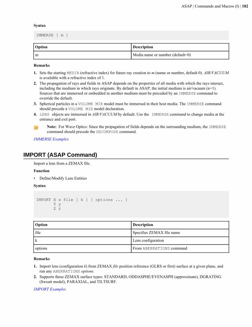
ASAP | Commands and Macros (I) | 182
Syntax
IMMERSE [ m ]
Option Description
m Media name or number (default=0)
Remarks
1. Sets the starting MEDIA (refractive index) for future ray creation to m (name or number, default 0). AIR/VACUUMis available with a refractive index of 1.
2. The propagation of rays and fields in ASAP depends on the properties of all media with which the rays interact,including the medium in which rays originate. By default in ASAP, the initial medium is air/vacuum (n=1).Sources that are immersed or embedded in another medium must be preceded by an IMMERSE command tooverride the default.
3. Spherical particles in a VOLUME MIE model must be immersed in their host media. The IMMERSE commandshould precede a VOLUME MIE model declaration.
4. LENS objects are immersed in AIR/VACUUM by default. Use the IMMERSE command to change media at theentrance and exit port.
Note: For Wave Optics: Since the propagation of fields depends on the surrounding medium, the IMMERSEcommand should precede the DECOMPOSE command.
IMMERSE Examples
IMPORT (ASAP Command)Import a lens from a ZEMAX file.
Function
• Define/Modify Lens Entities
Syntax
IMPORT X x file [ k ] [ options ... ] Y y Z z
Option Description
file Specifies ZEMAX file name
k Lens configuration
options From ABERRATIONS command
Remarks
1. Import lens (configuration k) from ZEMAX file position reference (GLRS or first) surface at a given plane, andrun any ABERRATIONS options.
2. Supports these ZEMAX surface types: STANDARD, ODDASPHE/EVENASPH (approximate), DGRATING(Sweatt model), PARAXIAL, and TILTSURF.
IMPORT Examples
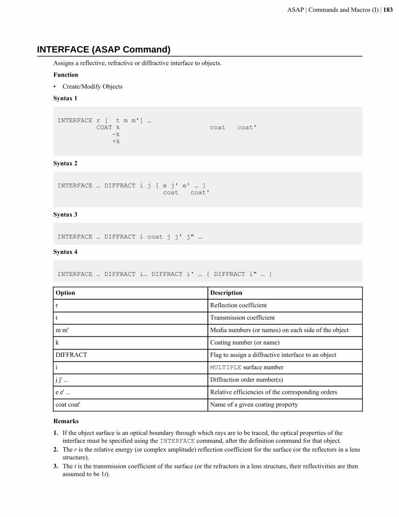
ASAP | Commands and Macros (I) | 183
INTERFACE (ASAP Command)Assigns a reflective, refractive or diffractive interface to objects.
Function
• Create/Modify Objects
Syntax 1
INTERFACE r [ t m m'] … COAT k coat coat' -k +k
Syntax 2
INTERFACE … DIFFRACT i j [ e j' e' … ] coat coat'
Syntax 3
INTERFACE … DIFFRACT i coat j j' j" …
Syntax 4
INTERFACE … DIFFRACT i… DIFFRACT i' … [ DIFFRACT i" … ]
Option Description
r Reflection coefficient
t Transmission coefficient
m m' Media numbers (or names) on each side of the object
k Coating number (or name)
DIFFRACT Flag to assign a diffractive interface to an object
i MULTIPLE surface number
j j' ... Diffraction order number(s)
e e' ... Relative efficiencies of the corresponding orders
coat coat' Name of a given coating property
Remarks
1. If the object surface is an optical boundary through which rays are to be traced, the optical properties of theinterface must be specified using the INTERFACE command, after the definition command for that object.
2. The r is the relative energy (or complex amplitude) reflection coefficient for the surface (or the reflectors in a lensstructure).
3. The t is the transmission coefficient of the surface (or the refractors in a lens structure, their reflectivities are thenassumed to be 1t).
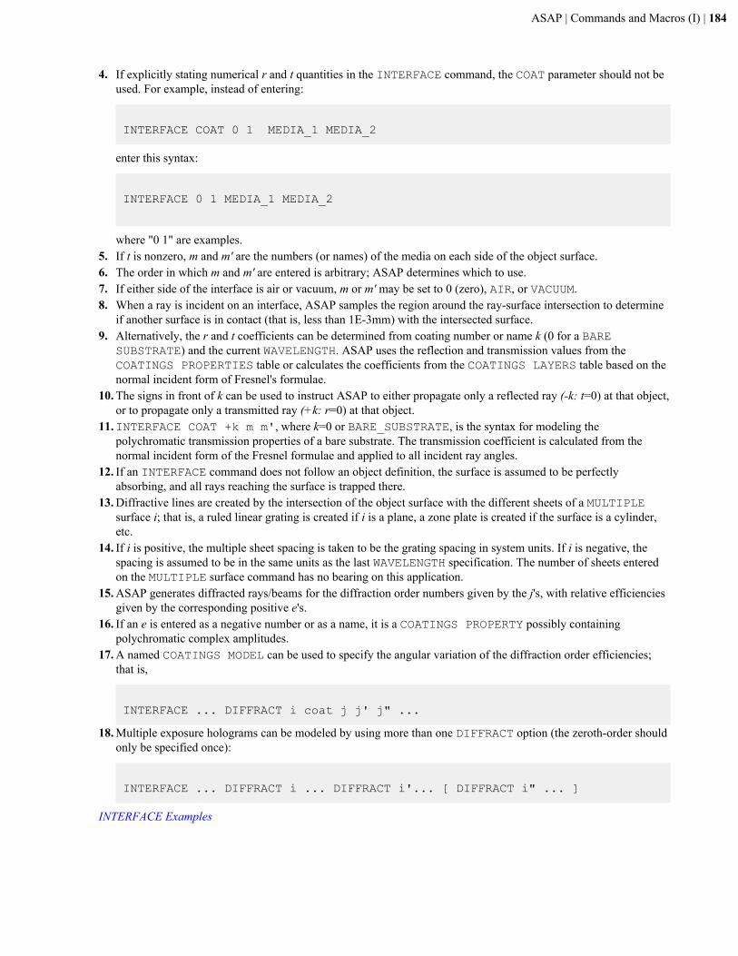
ASAP | Commands and Macros (I) | 184
4. If explicitly stating numerical r and t quantities in the INTERFACE command, the COAT parameter should not beused. For example, instead of entering:
INTERFACE COAT 0 1 MEDIA_1 MEDIA_2
enter this syntax:
INTERFACE 0 1 MEDIA_1 MEDIA_2
where "0 1" are examples.5. If t is nonzero, m and m' are the numbers (or names) of the media on each side of the object surface.6. The order in which m and m' are entered is arbitrary; ASAP determines which to use.7. If either side of the interface is air or vacuum, m or m' may be set to 0 (zero), AIR, or VACUUM.8. When a ray is incident on an interface, ASAP samples the region around the ray-surface intersection to determine
if another surface is in contact (that is, less than 1E-3mm) with the intersected surface.9. Alternatively, the r and t coefficients can be determined from coating number or name k (0 for a BARE
SUBSTRATE) and the current WAVELENGTH. ASAP uses the reflection and transmission values from theCOATINGS PROPERTIES table or calculates the coefficients from the COATINGS LAYERS table based on thenormal incident form of Fresnel's formulae.
10. The signs in front of k can be used to instruct ASAP to either propagate only a reflected ray (-k: t=0) at that object,or to propagate only a transmitted ray (+k: r=0) at that object.
11.INTERFACE COAT +k m m', where k=0 or BARE_SUBSTRATE, is the syntax for modeling thepolychromatic transmission properties of a bare substrate. The transmission coefficient is calculated from thenormal incident form of the Fresnel formulae and applied to all incident ray angles.
12. If an INTERFACE command does not follow an object definition, the surface is assumed to be perfectlyabsorbing, and all rays reaching the surface is trapped there.
13. Diffractive lines are created by the intersection of the object surface with the different sheets of a MULTIPLEsurface i; that is, a ruled linear grating is created if i is a plane, a zone plate is created if the surface is a cylinder,etc.
14. If i is positive, the multiple sheet spacing is taken to be the grating spacing in system units. If i is negative, thespacing is assumed to be in the same units as the last WAVELENGTH specification. The number of sheets enteredon the MULTIPLE surface command has no bearing on this application.
15. ASAP generates diffracted rays/beams for the diffraction order numbers given by the j's, with relative efficienciesgiven by the corresponding positive e's.
16. If an e is entered as a negative number or as a name, it is a COATINGS PROPERTY possibly containingpolychromatic complex amplitudes.
17. A named COATINGS MODEL can be used to specify the angular variation of the diffraction order efficiencies;that is,
INTERFACE ... DIFFRACT i coat j j' j" ...
18. Multiple exposure holograms can be modeled by using more than one DIFFRACT option (the zeroth-order shouldonly be specified once):
INTERFACE ... DIFFRACT i ... DIFFRACT i'... [ DIFFRACT i" ... ]
INTERFACE Examples
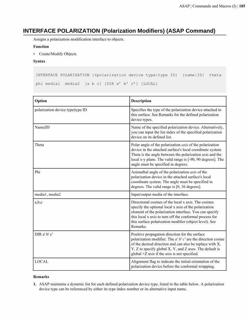
ASAP | Commands and Macros (I) | 185
INTERFACE POLARIZATION (Polarization Modifiers) (ASAP Command)Assigns a polarization modification interface to objects.
Function
• Create/Modify Objects
Syntax
INTERFACE POLARIZATION {±polarization device type|type ID} {name|ID} theta phi media1 media2 [a b c] [DIR a’ b’ c’] [LOCAL]
Option Description
polarization device type|type ID Specifies the type of the polarization device attached tothis surface. See Remarks for the defined polarizationdevice types.
Name|ID Name of the specified polarization device. Alternatively,you can input the list index of the specified polarizationdevice on its defined list.
Theta Polar angle of the polarization axis of the polarizationdevice in the attached surface's local coordinate system.Theta is the angle between the polarization axis and thelocal x-y plane. The valid range is [-90, 90 degrees]. Theangle must be specified in degrees.
Phi Azimuthal angle of the polarization axis of thepolarization device in the attached surface's localcoordinate system. The angle must be specified indegrees. The valid range is [0, 36 degrees].
media1, media2 Input/output media of the interface.
a,b,c Directional cosines of the local x axis. The cosinesspecify the optional local x axis of the polarizationelement of the polarization interface. You can specifythis local x axis to turn off the conformal process forthis surface polarization modifier (object level). SeeRemarks.
DIR a' b' c' Positive propagation direction for the surfacepolarization modifier. The a' b' c' are the direction cosineof the desired direction and can also be replace with X,Y, Z to specify global X, Y, and Z axes. The default isglobal +Z axis if the axis is not specified.
LOCAL Alignment flag to indicate the initial orientation of thepolarization device before the conformal wrapping.
Remarks
1. ASAP maintains a dynamic list for each defined polarization device type, listed in the table below. A polarizationdevice type can be referenced by either its type index number or its alternative input name.
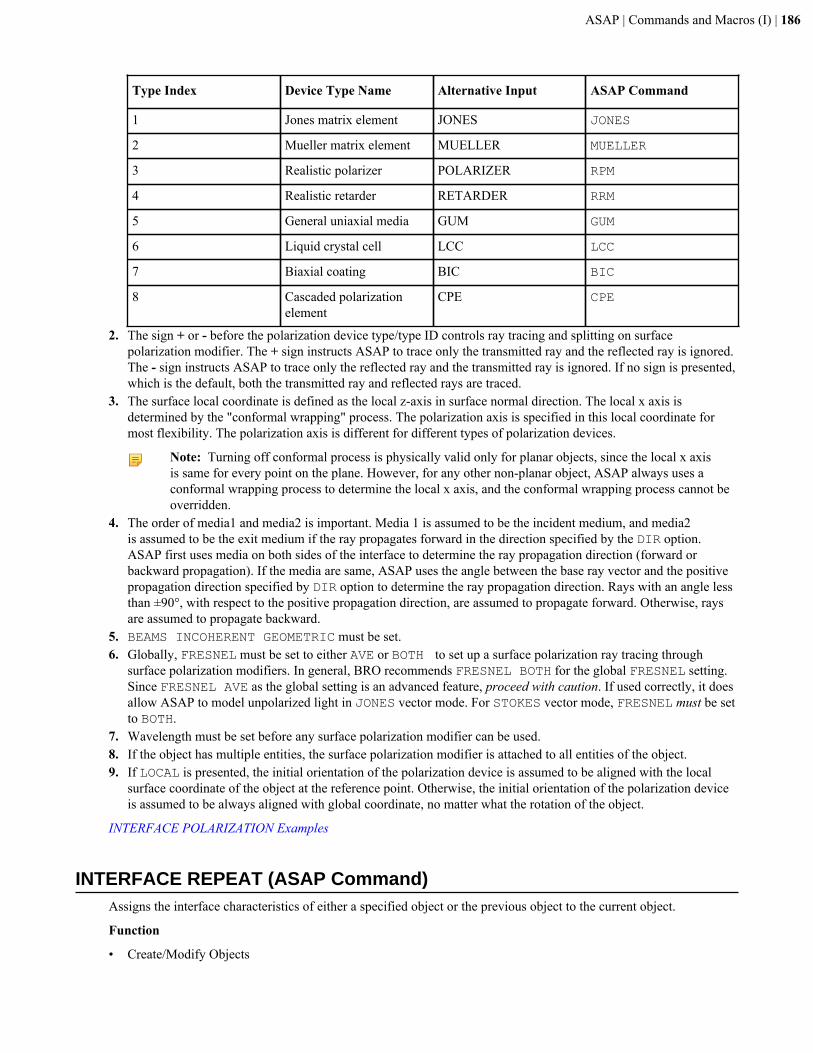
ASAP | Commands and Macros (I) | 186
Type Index Device Type Name Alternative Input ASAP Command
1 Jones matrix element JONES JONES
2 Mueller matrix element MUELLER MUELLER
3 Realistic polarizer POLARIZER RPM
4 Realistic retarder RETARDER RRM
5 General uniaxial media GUM GUM
6 Liquid crystal cell LCC LCC
7 Biaxial coating BIC BIC
8 Cascaded polarizationelement
CPE CPE
2. The sign + or - before the polarization device type/type ID controls ray tracing and splitting on surfacepolarization modifier. The + sign instructs ASAP to trace only the transmitted ray and the reflected ray is ignored.The - sign instructs ASAP to trace only the reflected ray and the transmitted ray is ignored. If no sign is presented,which is the default, both the transmitted ray and reflected rays are traced.
3. The surface local coordinate is defined as the local z-axis in surface normal direction. The local x axis isdetermined by the "conformal wrapping" process. The polarization axis is specified in this local coordinate formost flexibility. The polarization axis is different for different types of polarization devices.
Note: Turning off conformal process is physically valid only for planar objects, since the local x axisis same for every point on the plane. However, for any other non-planar object, ASAP always uses aconformal wrapping process to determine the local x axis, and the conformal wrapping process cannot beoverridden.
4. The order of media1 and media2 is important. Media 1 is assumed to be the incident medium, and media2is assumed to be the exit medium if the ray propagates forward in the direction specified by the DIR option.ASAP first uses media on both sides of the interface to determine the ray propagation direction (forward orbackward propagation). If the media are same, ASAP uses the angle between the base ray vector and the positivepropagation direction specified by DIR option to determine the ray propagation direction. Rays with an angle lessthan ±90°, with respect to the positive propagation direction, are assumed to propagate forward. Otherwise, raysare assumed to propagate backward.
5. BEAMS INCOHERENT GEOMETRIC must be set.6. Globally, FRESNEL must be set to either AVE or BOTH to set up a surface polarization ray tracing through
surface polarization modifiers. In general, BRO recommends FRESNEL BOTH for the global FRESNEL setting.Since FRESNEL AVE as the global setting is an advanced feature, proceed with caution. If used correctly, it doesallow ASAP to model unpolarized light in JONES vector mode. For STOKES vector mode, FRESNEL must be setto BOTH.
7. Wavelength must be set before any surface polarization modifier can be used.8. If the object has multiple entities, the surface polarization modifier is attached to all entities of the object.9. If LOCAL is presented, the initial orientation of the polarization device is assumed to be aligned with the local
surface coordinate of the object at the reference point. Otherwise, the initial orientation of the polarization deviceis assumed to be always aligned with global coordinate, no matter what the rotation of the object.
INTERFACE POLARIZATION Examples
INTERFACE REPEAT (ASAP Command)Assigns the interface characteristics of either a specified object or the previous object to the current object.
Function
• Create/Modify Objects
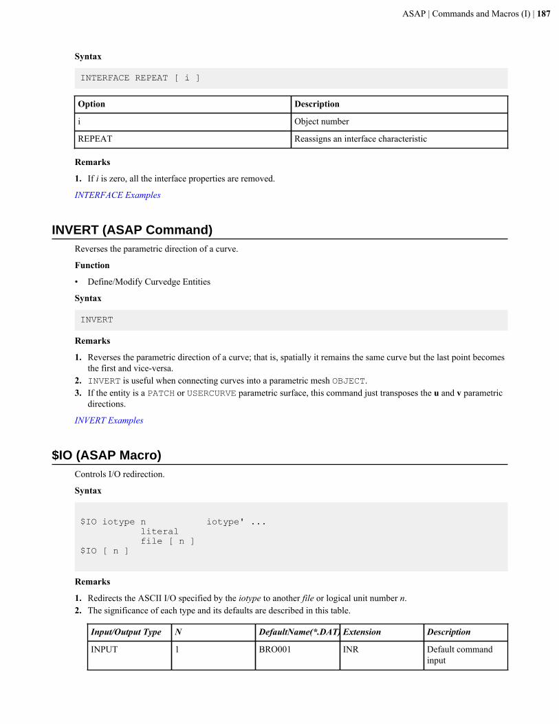
ASAP | Commands and Macros (I) | 187
Syntax
INTERFACE REPEAT [ i ]
Option Description
i Object number
REPEAT Reassigns an interface characteristic
Remarks
1. If i is zero, all the interface properties are removed.
INTERFACE Examples
INVERT (ASAP Command)Reverses the parametric direction of a curve.
Function
• Define/Modify Curvedge Entities
Syntax
INVERT
Remarks
1. Reverses the parametric direction of a curve; that is, spatially it remains the same curve but the last point becomesthe first and vice-versa.
2. INVERT is useful when connecting curves into a parametric mesh OBJECT.3. If the entity is a PATCH or USERCURVE parametric surface, this command just transposes the u and v parametric
directions.
INVERT Examples
$IO (ASAP Macro)Controls I/O redirection.
Syntax
$IO iotype n iotype' ... literal file [ n ]$IO [ n ]
Remarks
1. Redirects the ASCII I/O specified by the iotype to another file or logical unit number n.2. The significance of each type and its defaults are described in this table.
Input/Output Type N DefaultName(*.DAT) Extension Description
INPUT 1 BRO001 INR Default commandinput
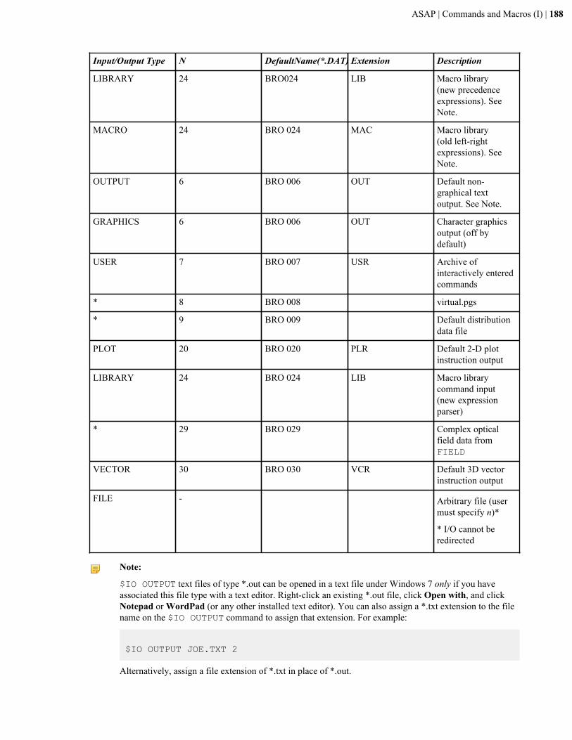
ASAP | Commands and Macros (I) | 188
Input/Output Type N DefaultName(*.DAT) Extension Description
LIBRARY 24 BRO024 LIB Macro library(new precedenceexpressions). SeeNote.
MACRO 24 BRO 024 MAC Macro library(old left-rightexpressions). SeeNote.
OUTPUT 6 BRO 006 OUT Default non-graphical textoutput. See Note.
GRAPHICS 6 BRO 006 OUT Character graphicsoutput (off bydefault)
USER 7 BRO 007 USR Archive ofinteractively enteredcommands
* 8 BRO 008 virtual.pgs
* 9 BRO 009 Default distributiondata file
PLOT 20 BRO 020 PLR Default 2-D plotinstruction output
LIBRARY 24 BRO 024 LIB Macro librarycommand input(new expressionparser)
* 29 BRO 029 Complex opticalfield data fromFIELD
VECTOR 30 BRO 030 VCR Default 3D vectorinstruction output
FILE - Arbitrary file (usermust specify n)*
* I/O cannot beredirected
Note:
$IO OUTPUT text files of type *.out can be opened in a text file under Windows 7 only if you haveassociated this file type with a text editor. Right-click an existing *.out file, click Open with, and clickNotepad or WordPad (or any other installed text editor). You can also assign a *.txt extension to the filename on the $IO OUTPUT command to assign that extension. For example:
$IO OUTPUT JOE.TXT 2
Alternatively, assign a file extension of *.txt in place of *.out.
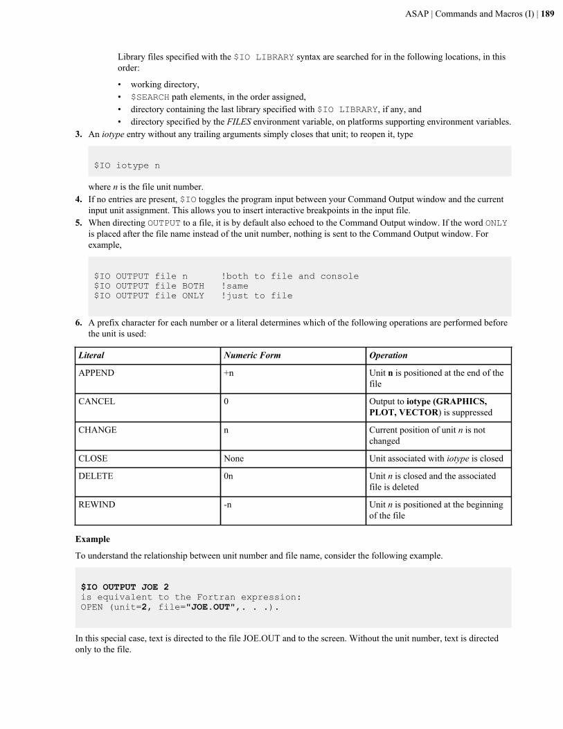
ASAP | Commands and Macros (I) | 189
Library files specified with the $IO LIBRARY syntax are searched for in the following locations, in thisorder:
• working directory,• $SEARCH path elements, in the order assigned,• directory containing the last library specified with $IO LIBRARY, if any, and• directory specified by the FILES environment variable, on platforms supporting environment variables.
3. An iotype entry without any trailing arguments simply closes that unit; to reopen it, type
$IO iotype n
where n is the file unit number.4. If no entries are present, $IO toggles the program input between your Command Output window and the current
input unit assignment. This allows you to insert interactive breakpoints in the input file.5. When directing OUTPUT to a file, it is by default also echoed to the Command Output window. If the word ONLY
is placed after the file name instead of the unit number, nothing is sent to the Command Output window. Forexample,
$IO OUTPUT file n !both to file and console$IO OUTPUT file BOTH !same$IO OUTPUT file ONLY !just to file
6. A prefix character for each number or a literal determines which of the following operations are performed beforethe unit is used:
Literal Numeric Form Operation
APPEND +n Unit n is positioned at the end of thefile
CANCEL 0 Output to iotype (GRAPHICS,PLOT, VECTOR) is suppressed
CHANGE n Current position of unit n is notchanged
CLOSE None Unit associated with iotype is closed
DELETE 0n Unit n is closed and the associatedfile is deleted
REWIND -n Unit n is positioned at the beginningof the file
Example
To understand the relationship between unit number and file name, consider the following example.
$IO OUTPUT JOE 2 is equivalent to the Fortran expression:OPEN (unit=2, file="JOE.OUT",. . .).
In this special case, text is directed to the file JOE.OUT and to the screen. Without the unit number, text is directedonly to the file.
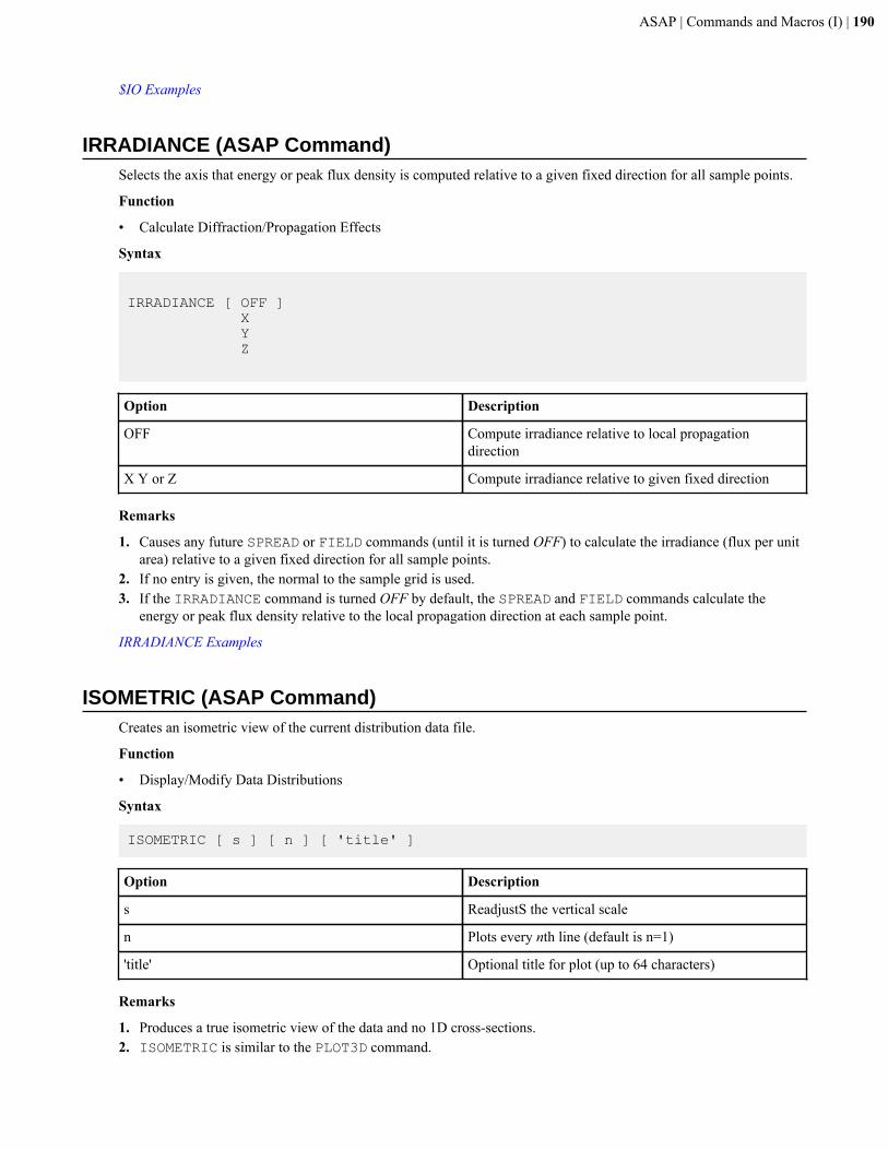
ASAP | Commands and Macros (I) | 190
$IO Examples
IRRADIANCE (ASAP Command)Selects the axis that energy or peak flux density is computed relative to a given fixed direction for all sample points.
Function
• Calculate Diffraction/Propagation Effects
Syntax
IRRADIANCE [ OFF ] X Y Z
Option Description
OFF Compute irradiance relative to local propagationdirection
X Y or Z Compute irradiance relative to given fixed direction
Remarks
1. Causes any future SPREAD or FIELD commands (until it is turned OFF) to calculate the irradiance (flux per unitarea) relative to a given fixed direction for all sample points.
2. If no entry is given, the normal to the sample grid is used.3. If the IRRADIANCE command is turned OFF by default, the SPREAD and FIELD commands calculate the
energy or peak flux density relative to the local propagation direction at each sample point.
IRRADIANCE Examples
ISOMETRIC (ASAP Command)Creates an isometric view of the current distribution data file.
Function
• Display/Modify Data Distributions
Syntax
ISOMETRIC [ s ] [ n ] [ 'title' ]
Option Description
s ReadjustS the vertical scale
n Plots every nth line (default is n=1)
'title' Optional title for plot (up to 64 characters)
Remarks
1. Produces a true isometric view of the data and no 1D cross-sections.2. ISOMETRIC is similar to the PLOT3D command.
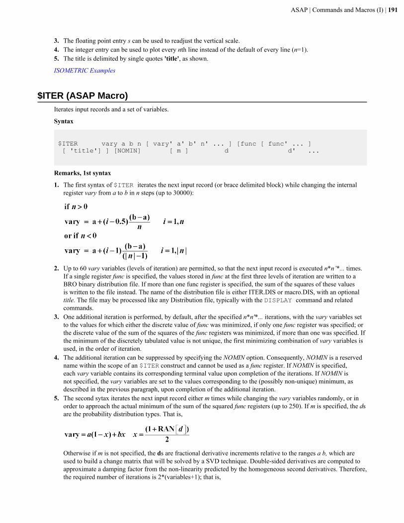
ASAP | Commands and Macros (I) | 191
3. The floating point entry s can be used to readjust the vertical scale.4. The integer entry can be used to plot every nth line instead of the default of every line (n=1).5. The title is delimited by single quotes 'title', as shown.
ISOMETRIC Examples
$ITER (ASAP Macro)Iterates input records and a set of variables.
Syntax
$ITER vary a b n [ vary' a' b' n' ... ] [func [ func' ... ] [ 'title'] ] [NOMIN] [ m ] d d' ...
Remarks, 1st syntax
1. The first syntax of $ITER iterates the next input record (or brace delimited block) while changing the internalregister vary from a to b in n steps (up to 30000):
2. Up to 60 vary variables (levels of iteration) are permitted, so that the next input record is executed n*n’*... times.If a single register func is specified, the values stored in func at the first three levels of iteration are written to aBRO binary distribution file. If more than one func register is specified, the sum of the squares of these valuesis written to the file instead. The name of the distribution file is either ITER.DIS or macro.DIS, with an optionaltitle. The file may be processed like any Distribution file, typically with the DISPLAY command and relatedcommands.
3. One additional iteration is performed, by default, after the specified n*n'*... iterations, with the vary variables setto the values for which either the discrete value of func was minimized, if only one func register was specified; orthe discrete value of the sum of the squares of the func registers was minimized, if more than one was specified. Ifthe minimum of the discretely tabulated value is not unique, the first minimizing combination of vary variables isused, in the order of iteration.
4. The additional iteration can be suppressed by specifying the NOMIN option. Consequently, NOMIN is a reservedname within the scope of an $ITER construct and cannot be used as a func register. If NOMIN is specified,each vary variable contains its corresponding terminal value upon completion of the iterations. If NOMIN isnot specified, the vary variables are set to the values corresponding to the (possibly non-unique) minimum, asdescribed in the previous paragraph, upon completion of the additional iteration.
5. The second sytax iterates the next input record either m times while changing the vary variables randomly, or inorder to approach the actual minimum of the sum of the squared func registers (up to 250). If m is specified, the dsare the probability distribution types. That is,
Otherwise if m is not specified, the ds are fractional derivative increments relative to the ranges a b, which areused to build a change matrix that will be solved by a SVD technique. Double-sided derivatives are computed toapproximate a damping factor from the non-linearity predicted by the homogeneous second derivatives. Therefore,the required number of iterations is 2*(variables+1); that is,
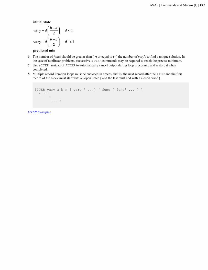
ASAP | Commands and Macros (I) | 192
6. The number of funcs should be greater than (>) or equal to (=) the number of vary's to find a unique solution. Inthe case of nonlinear problems, successive $ITER commands may be required to reach the precise minimum.
7. Use &ITER instead of $ITER to automatically cancel output during loop processing and restore it whencompleted.
8. Multiple record iteration loops must be enclosed in braces; that is, the next record after the ITER and the firstrecord of the block must start with an open brace { and the last must end with a closed brace }.
$ITER vary a b n [ vary ' ...] [ func [ func' ... ] ] { ... : ... }
$ITER Examples
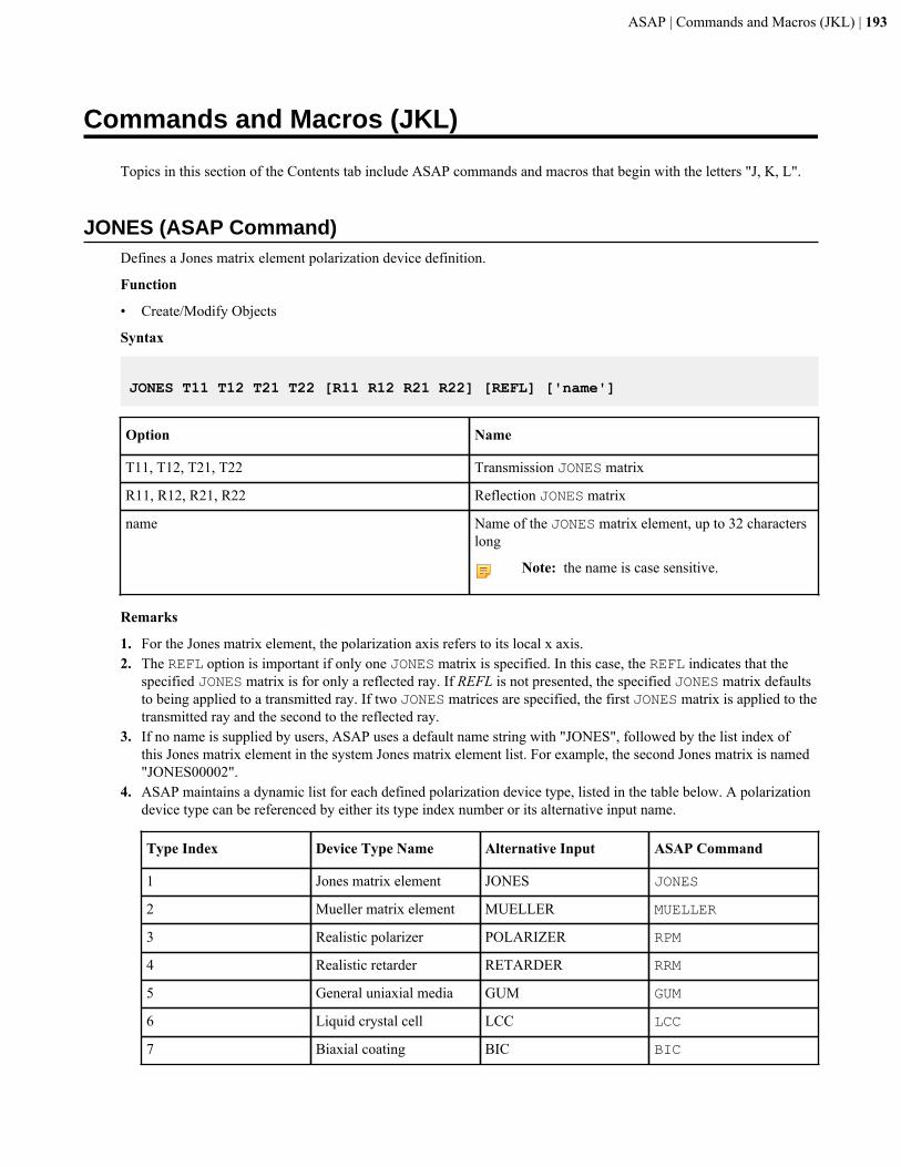
ASAP | Commands and Macros (JKL) | 193
Commands and Macros (JKL)
Topics in this section of the Contents tab include ASAP commands and macros that begin with the letters "J, K, L".
JONES (ASAP Command)Defines a Jones matrix element polarization device definition.
Function
• Create/Modify Objects
Syntax
JONES T11 T12 T21 T22 [R11 R12 R21 R22] [REFL] ['name']
Option Name
T11, T12, T21, T22 Transmission JONES matrix
R11, R12, R21, R22 Reflection JONES matrix
name Name of the JONES matrix element, up to 32 characterslong
Note: the name is case sensitive.
Remarks
1. For the Jones matrix element, the polarization axis refers to its local x axis.2. The REFL option is important if only one JONES matrix is specified. In this case, the REFL indicates that the
specified JONES matrix is for only a reflected ray. If REFL is not presented, the specified JONES matrix defaultsto being applied to a transmitted ray. If two JONES matrices are specified, the first JONES matrix is applied to thetransmitted ray and the second to the reflected ray.
3. If no name is supplied by users, ASAP uses a default name string with "JONES", followed by the list index ofthis Jones matrix element in the system Jones matrix element list. For example, the second Jones matrix is named"JONES00002".
4. ASAP maintains a dynamic list for each defined polarization device type, listed in the table below. A polarizationdevice type can be referenced by either its type index number or its alternative input name.
Type Index Device Type Name Alternative Input ASAP Command
1 Jones matrix element JONES JONES
2 Mueller matrix element MUELLER MUELLER
3 Realistic polarizer POLARIZER RPM
4 Realistic retarder RETARDER RRM
5 General uniaxial media GUM GUM
6 Liquid crystal cell LCC LCC
7 Biaxial coating BIC BIC
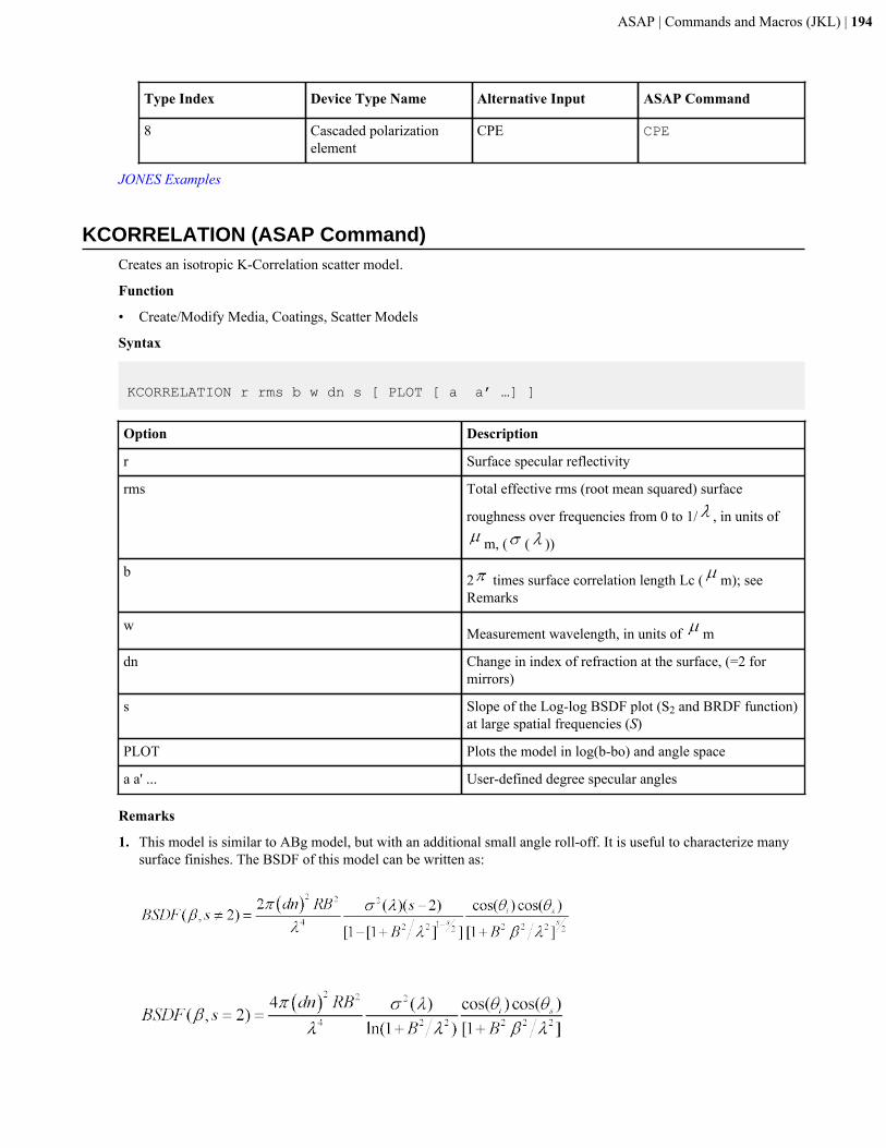
ASAP | Commands and Macros (JKL) | 194
Type Index Device Type Name Alternative Input ASAP Command
8 Cascaded polarizationelement
CPE CPE
JONES Examples
KCORRELATION (ASAP Command)Creates an isotropic K-Correlation scatter model.
Function
• Create/Modify Media, Coatings, Scatter Models
Syntax
KCORRELATION r rms b w dn s [ PLOT [ a a’ …] ]
Option Description
r Surface specular reflectivity
rms Total effective rms (root mean squared) surface
roughness over frequencies from 0 to 1/ , in units of
m, ( ( ))
b 2 times surface correlation length Lc ( m); seeRemarks
w Measurement wavelength, in units of m
dn Change in index of refraction at the surface, (=2 formirrors)
s Slope of the Log-log BSDF plot (S2 and BRDF function)at large spatial frequencies (S)
PLOT Plots the model in log(b-bo) and angle space
a a' ... User-defined degree specular angles
Remarks
1. This model is similar to ABg model, but with an additional small angle roll-off. It is useful to characterize manysurface finishes. The BSDF of this model can be written as:

ASAP | Commands and Macros (JKL) | 195
Note: See the technical guide, "Scattering in ASAP" on the Knowledge Base for more information on thisfeature.
2. May be used with importance area sampling.3. The w is the wavelength (in unit of m) at which this model is defined (or was measured).4. Command argument, PLOT plots the model (common base 10 logarithm of the BSDF) for up to seven specular
angles in ascending order (default 0, 15, 30, 45, 60, 75, 89.9 degrees). The current PIXELS setting controls theresolution of these plots in direction cosine space, and creates a distribution file, name_angle.dis, for each of theseangles.
5. The command argument, MINMAX can be used to set the minimum and maximum values of the BSDF for thisspecific model.
KCORRELATION Examples
LAMBERTIAN (ASAP Command)Creates a Lambertian scatter model.
Function
• Create/Modify Media, Coatings, Scatter Models
Syntax
LAMBERTIAN t [ PLOT [ a a' ... ] ]
Option Description
t Total hemispherical diffuse scatter ratio (<1 or =1)
PLOT Plots the model in log(b-bo) and angle space
a a' ... User-defined degree specular angles
Remarks
1. Use with importance area sampling.2. The PLOT option plots the model (common base 10 logarithm of the BSDF) for up to seven specular angles in
ascending order (default 0, 15, 30, 45, 60, 75, 89.9 degrees). The current PIXELS setting controls the resolutionof these plots in direction cosine space.
3. The BSDF is independent of wavelength, incidence direction, and scatter direction.4. Creates a distribution file name_angle.dis for each of these angles.5. The command argument, MINMAX may be used to set the minimum and maximum values of the BSDF for this
specific model.6. t does not affect ROUGHNESS models, but is still necessary for the command to run. You may leave the value as
1.
LAMBERTIAN Examples
LCC (ASAP Command)Defines a liquid crystal cell (LCC) layer device model. The LCC accurately models both on- and off-axis propagationof polarized light inside a crystal.
Function
• Create/Modify Objects
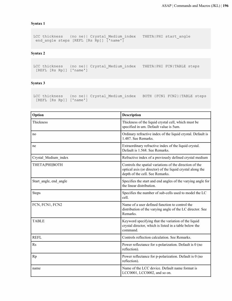
ASAP | Commands and Macros (JKL) | 196
Syntax 1
LCC thickness {no ne}| Crystal_Medium_index THETA|PHI start_angle end_angle steps [REFL [Rs Rp]] ['name']
Syntax 2
LCC thickness {no ne}| Crystal_Medium_index THETA|PHI FCN|TABLE steps [REFL [Rs Rp]] ['name']
Syntax 3
LCC thickness {no ne}| Crystal_Medium_index BOTH {FCN1 FCN2}|TABLE steps [REFL [Rs Rp]] ['name']
Option Description
Thickness Thickness of the liquid crystal cell, which must bespecified in um. Default value is 5um.
no Ordinary refractive index of the liquid crystal. Default is1.487. See Remarks.
ne Extraordinary refractive index of the liquid crystal.Default is 1.568. See Remarks.
Crystal_Medium_index Refractive index of a previously defined crystal medium
THETA|PHI|BOTH Controls the spatial variations of the direction of theoptical axis (or director) of the liquid crystal along thedepth of the cell. See Remarks.
Start_angle, end_angle Specifies the start and end angles of the varying angle forthe linear distribution.
Steps Specifies the number of sub-cells used to model the LCcell.
FCN, FCN1, FCN2 Name of a user defined function to control thedistribution of the varying angle of the LC director. SeeRemarks.
TABLE Keyword specifying that the variation of the liquidcrystal director, which is listed in a table below thecommand.
REFL Controls reflection calculation. See Remarks.
Rs Power reflectance for s-polarization. Default is 0 (noreflection).
Rp Power reflectance for p-polarization. Default is 0 (noreflection).
name Name of the LCC device. Default name format isLCC0001, LCC0002, and so on.
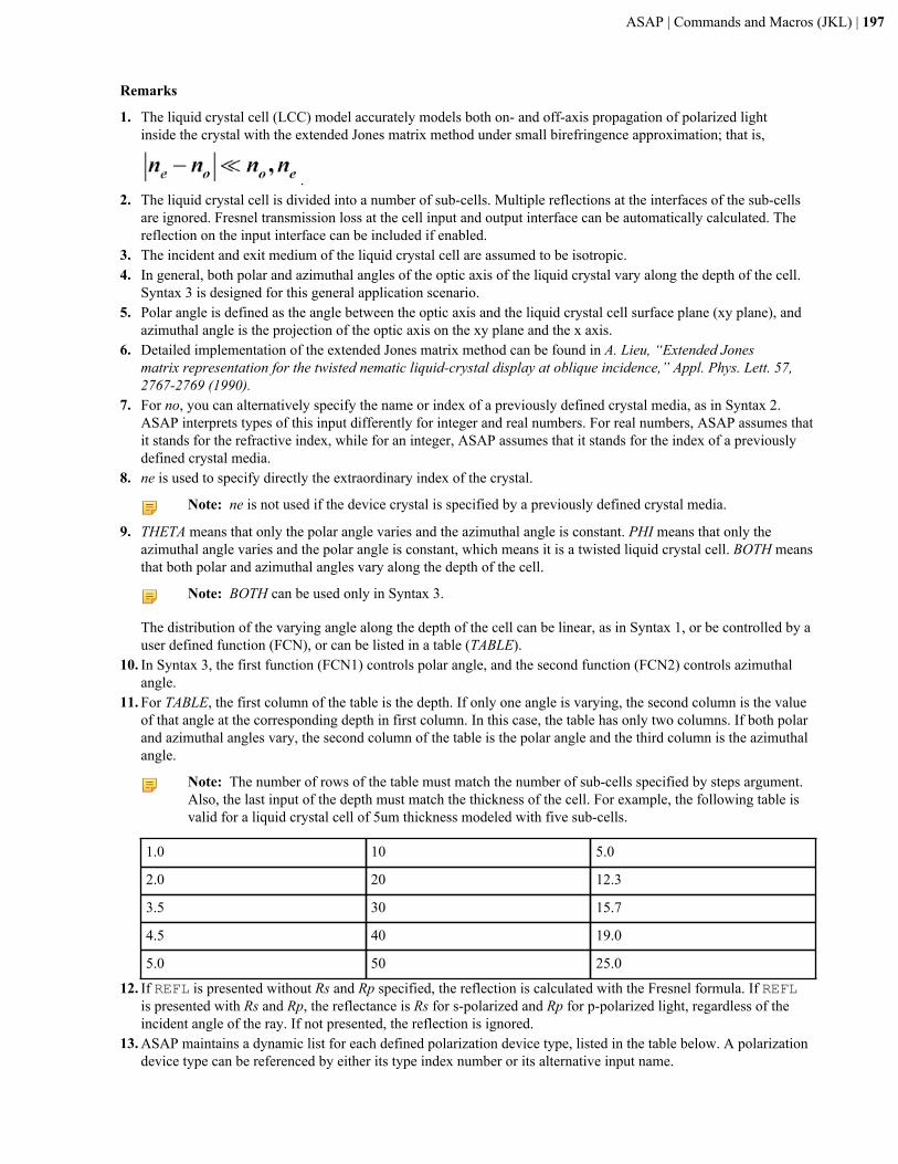
ASAP | Commands and Macros (JKL) | 197
Remarks
1. The liquid crystal cell (LCC) model accurately models both on- and off-axis propagation of polarized lightinside the crystal with the extended Jones matrix method under small birefringence approximation; that is,
.2. The liquid crystal cell is divided into a number of sub-cells. Multiple reflections at the interfaces of the sub-cells
are ignored. Fresnel transmission loss at the cell input and output interface can be automatically calculated. Thereflection on the input interface can be included if enabled.
3. The incident and exit medium of the liquid crystal cell are assumed to be isotropic.4. In general, both polar and azimuthal angles of the optic axis of the liquid crystal vary along the depth of the cell.
Syntax 3 is designed for this general application scenario.5. Polar angle is defined as the angle between the optic axis and the liquid crystal cell surface plane (xy plane), and
azimuthal angle is the projection of the optic axis on the xy plane and the x axis.6. Detailed implementation of the extended Jones matrix method can be found in A. Lieu, “Extended Jones
matrix representation for the twisted nematic liquid-crystal display at oblique incidence,” Appl. Phys. Lett. 57,2767-2769 (1990).
7. For no, you can alternatively specify the name or index of a previously defined crystal media, as in Syntax 2.ASAP interprets types of this input differently for integer and real numbers. For real numbers, ASAP assumes thatit stands for the refractive index, while for an integer, ASAP assumes that it stands for the index of a previouslydefined crystal media.
8. ne is used to specify directly the extraordinary index of the crystal.
Note: ne is not used if the device crystal is specified by a previously defined crystal media.
9. THETA means that only the polar angle varies and the azimuthal angle is constant. PHI means that only theazimuthal angle varies and the polar angle is constant, which means it is a twisted liquid crystal cell. BOTH meansthat both polar and azimuthal angles vary along the depth of the cell.
Note: BOTH can be used only in Syntax 3.
The distribution of the varying angle along the depth of the cell can be linear, as in Syntax 1, or be controlled by auser defined function (FCN), or can be listed in a table (TABLE).
10. In Syntax 3, the first function (FCN1) controls polar angle, and the second function (FCN2) controls azimuthalangle.
11. For TABLE, the first column of the table is the depth. If only one angle is varying, the second column is the valueof that angle at the corresponding depth in first column. In this case, the table has only two columns. If both polarand azimuthal angles vary, the second column of the table is the polar angle and the third column is the azimuthalangle.
Note: The number of rows of the table must match the number of sub-cells specified by steps argument.Also, the last input of the depth must match the thickness of the cell. For example, the following table isvalid for a liquid crystal cell of 5um thickness modeled with five sub-cells.
1.0 10 5.0
2.0 20 12.3
3.5 30 15.7
4.5 40 19.0
5.0 50 25.0
12. If REFL is presented without Rs and Rp specified, the reflection is calculated with the Fresnel formula. If REFLis presented with Rs and Rp, the reflectance is Rs for s-polarized and Rp for p-polarized light, regardless of theincident angle of the ray. If not presented, the reflection is ignored.
13. ASAP maintains a dynamic list for each defined polarization device type, listed in the table below. A polarizationdevice type can be referenced by either its type index number or its alternative input name.
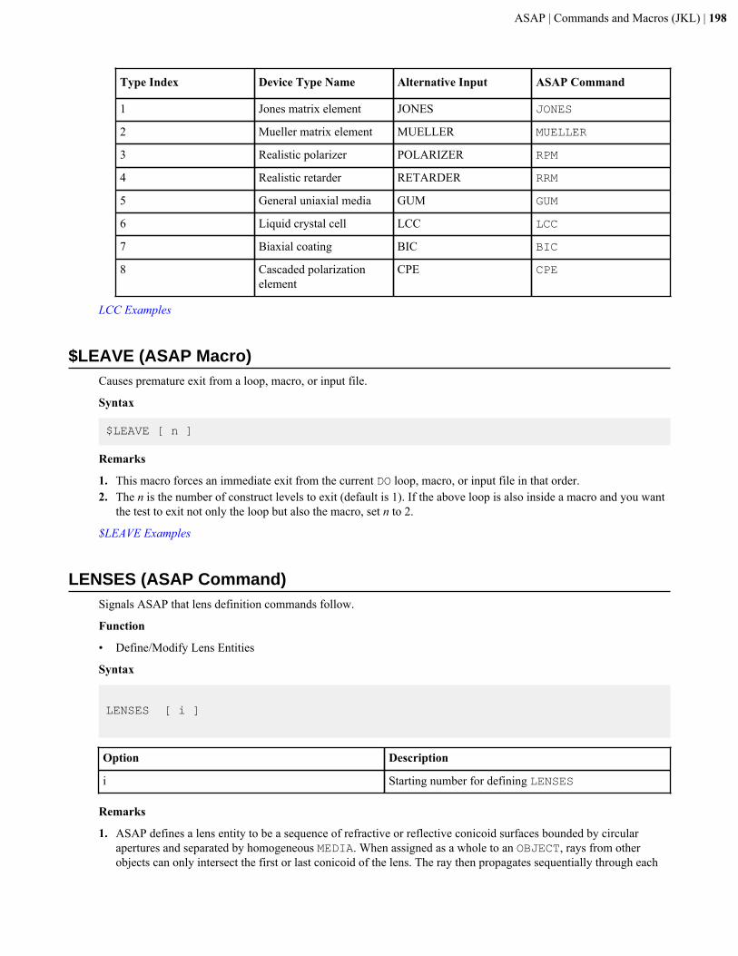
ASAP | Commands and Macros (JKL) | 198
Type Index Device Type Name Alternative Input ASAP Command
1 Jones matrix element JONES JONES
2 Mueller matrix element MUELLER MUELLER
3 Realistic polarizer POLARIZER RPM
4 Realistic retarder RETARDER RRM
5 General uniaxial media GUM GUM
6 Liquid crystal cell LCC LCC
7 Biaxial coating BIC BIC
8 Cascaded polarizationelement
CPE CPE
LCC Examples
$LEAVE (ASAP Macro)Causes premature exit from a loop, macro, or input file.
Syntax
$LEAVE [ n ]
Remarks
1. This macro forces an immediate exit from the current DO loop, macro, or input file in that order.2. The n is the number of construct levels to exit (default is 1). If the above loop is also inside a macro and you want
the test to exit not only the loop but also the macro, set n to 2.
$LEAVE Examples
LENSES (ASAP Command)Signals ASAP that lens definition commands follow.
Function
• Define/Modify Lens Entities
Syntax
LENSES [ i ]
Option Description
i Starting number for defining LENSES
Remarks
1. ASAP defines a lens entity to be a sequence of refractive or reflective conicoid surfaces bounded by circularapertures and separated by homogeneous MEDIA. When assigned as a whole to an OBJECT, rays from otherobjects can only intersect the first or last conicoid of the lens. The ray then propagates sequentially through each
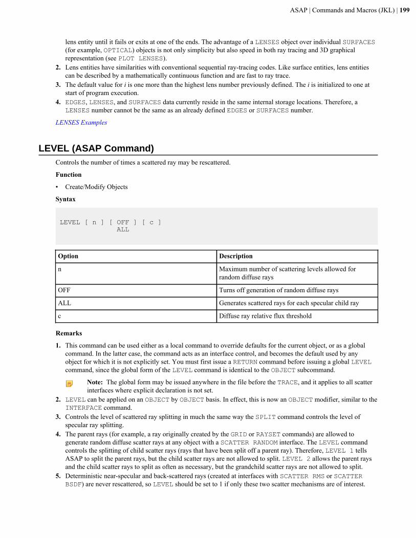
ASAP | Commands and Macros (JKL) | 199
lens entity until it fails or exits at one of the ends. The advantage of a LENSES object over individual SURFACES(for example, OPTICAL) objects is not only simplicity but also speed in both ray tracing and 3D graphicalrepresentation (see PLOT LENSES).
2. Lens entities have similarities with conventional sequential ray-tracing codes. Like surface entities, lens entitiescan be described by a mathematically continuous function and are fast to ray trace.
3. The default value for i is one more than the highest lens number previously defined. The i is initialized to one atstart of program execution.
4. EDGES, LENSES, and SURFACES data currently reside in the same internal storage locations. Therefore, aLENSES number cannot be the same as an already defined EDGES or SURFACES number.
LENSES Examples
LEVEL (ASAP Command)Controls the number of times a scattered ray may be rescattered.
Function
• Create/Modify Objects
Syntax
LEVEL [ n ] [ OFF ] [ c ] ALL
Option Description
n Maximum number of scattering levels allowed forrandom diffuse rays
OFF Turns off generation of random diffuse rays
ALL Generates scattered rays for each specular child ray
c Diffuse ray relative flux threshold
Remarks
1. This command can be used either as a local command to override defaults for the current object, or as a globalcommand. In the latter case, the command acts as an interface control, and becomes the default used by anyobject for which it is not explicitly set. You must first issue a RETURN command before issuing a global LEVELcommand, since the global form of the LEVEL command is identical to the OBJECT subcommand.
Note: The global form may be issued anywhere in the file before the TRACE, and it applies to all scatterinterfaces where explicit declaration is not set.
2. LEVEL can be applied on an OBJECT by OBJECT basis. In effect, this is now an OBJECT modifier, similar to theINTERFACE command.
3. Controls the level of scattered ray splitting in much the same way the SPLIT command controls the level ofspecular ray splitting.
4. The parent rays (for example, a ray originally created by the GRID or RAYSET commands) are allowed togenerate random diffuse scatter rays at any object with a SCATTER RANDOM interface. The LEVEL commandcontrols the splitting of child scatter rays (rays that have been split off a parent ray). Therefore, LEVEL 1 tellsASAP to split the parent rays, but the child scatter rays are not allowed to split. LEVEL 2 allows the parent raysand the child scatter rays to split as often as necessary, but the grandchild scatter rays are not allowed to split.
5. Deterministic near-specular and back-scattered rays (created at interfaces with SCATTER RMS or SCATTERBSDF) are never rescattered, so LEVEL should be set to 1 if only these two scatter mechanisms are of interest.
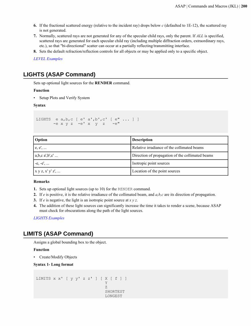
ASAP | Commands and Macros (JKL) | 200
6. If the fractional scattered energy (relative to the incident ray) drops below c (defaulted to 1E-12), the scattered rayis not generated.
7. Normally, scattered rays are not generated for any of the specular child rays, only the parent. If ALL is specified,scattered rays are generated for each specular child ray (including multiple diffraction orders, extraordinary rays,etc.), so that "bi-directional" scatter can occur at a partially reflecting/transmitting interface.
8. Sets the default refraction/reflection controls for all objects or may be applied only to a specific object.
LEVEL Examples
LIGHTS (ASAP Command)Sets up optional light sources for the RENDER command.
Function
• Setup Plots and Verify System
Syntax
LIGHTS e a,b,c [ e' a',b',c' [ e" ... ] ] -e x y z -e' x y z -e"
Option Description
e, e', ... Relative irradiance of the collimated beams
a,b,c a',b',c' ... Direction of propagation of the collimated beams
-e, -e', ... Isotropic point sources
x y z, x' y' z', ... Location of the point sources
Remarks
1. Sets up optional light sources (up to 10) for the RENDER command.2. If e is positive, it is the relative irradiance of the collimated beam, and a,b,c are its direction of propagation.3. If e is negative, the light is an isotropic point source at x y z.4. The addition of these light sources can significantly increase the time it takes to render a scene, because ASAP
must check for obscurations along the path of the light sources.
LIGHTS Examples
LIMITS (ASAP Command)Assigns a global bounding box to the object.
Function
• Create/Modify Objects
Syntax 1- Long format
LIMITS x x' [ y y' z z' ] [ X [ f ] ] Y Z SHORTEST LONGEST

ASAP | Commands and Macros (JKL) | 201
NORMAL
Syntax 2- Short format
LIMITS [ OFF ] REPEAT i [ X [ f ] ] STATS Y AXIS Z -X x SHORTEST -Y y LONGEST -Z z NORMAL +X x' OFF +Y y' +Z z' EXPAND r X r Y Z
Option Description
x x' Minimum and maximum extent in the global x direction
y y' Minimum and maximum extent in the global y direction
z z' Minimum and maximum extent in the global z direction
X, Y, or Z Coordinate direction
SHORTEST Coordinate axis determined by shortest limit boxdimension
LONGEST Coordinate axis determined by longest limit boxdimension
NORMAL Coordinate axis determined by coordinate directionnearest to the surface normal
OFF Makes limits a rectangular box nearest surface normal
f Fractional height of inner boundary (default=0)
LIMITS OFF Temporarily turn off future limits checking
REPEAT i Copies/repeats the limits box from object i
STATS Resets the limits box according to the previous TRACESTATS command
AXIS Resets the limits axis
-X x, -Y y, -Z z ... Specifies the specific bounding box side
EXPAND Scales the limits box
r Relative scale factor
Remarks
1. The minimum and maximum extents are defined in global coordinates.2. If the coordinate direction is not entered, the object is constrained by a rectangular box whose endpoints are given
by the minimum and maximum extent.
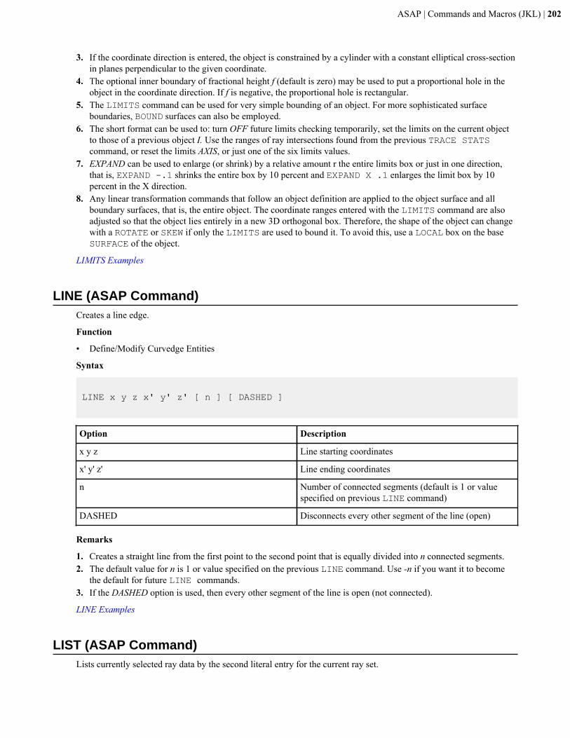
ASAP | Commands and Macros (JKL) | 202
3. If the coordinate direction is entered, the object is constrained by a cylinder with a constant elliptical cross-sectionin planes perpendicular to the given coordinate.
4. The optional inner boundary of fractional height f (default is zero) may be used to put a proportional hole in theobject in the coordinate direction. If f is negative, the proportional hole is rectangular.
5. The LIMITS command can be used for very simple bounding of an object. For more sophisticated surfaceboundaries, BOUND surfaces can also be employed.
6. The short format can be used to: turn OFF future limits checking temporarily, set the limits on the current objectto those of a previous object I. Use the ranges of ray intersections found from the previous TRACE STATScommand, or reset the limits AXIS, or just one of the six limits values.
7. EXPAND can be used to enlarge (or shrink) by a relative amount r the entire limits box or just in one direction,that is, EXPAND -.1 shrinks the entire box by 10 percent and EXPAND X .1 enlarges the limit box by 10percent in the X direction.
8. Any linear transformation commands that follow an object definition are applied to the object surface and allboundary surfaces, that is, the entire object. The coordinate ranges entered with the LIMITS command are alsoadjusted so that the object lies entirely in a new 3D orthogonal box. Therefore, the shape of the object can changewith a ROTATE or SKEW if only the LIMITS are used to bound it. To avoid this, use a LOCAL box on the baseSURFACE of the object.
LIMITS Examples
LINE (ASAP Command)Creates a line edge.
Function
• Define/Modify Curvedge Entities
Syntax
LINE x y z x' y' z' [ n ] [ DASHED ]
Option Description
x y z Line starting coordinates
x' y' z' Line ending coordinates
n Number of connected segments (default is 1 or valuespecified on previous LINE command)
DASHED Disconnects every other segment of the line (open)
Remarks
1. Creates a straight line from the first point to the second point that is equally divided into n connected segments.2. The default value for n is 1 or value specified on the previous LINE command. Use -n if you want it to become
the default for future LINE commands.3. If the DASHED option is used, then every other segment of the line is open (not connected).
LINE Examples
LIST (ASAP Command)Lists currently selected ray data by the second literal entry for the current ray set.
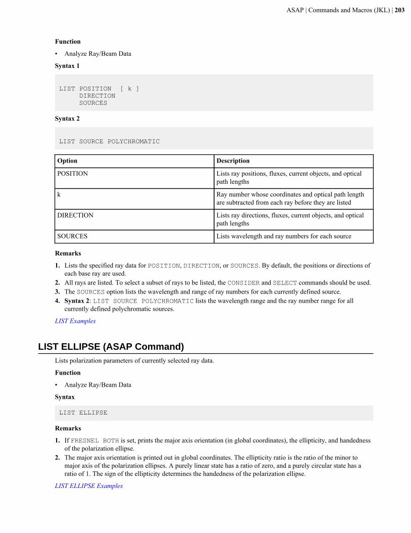
ASAP | Commands and Macros (JKL) | 203
Function
• Analyze Ray/Beam Data
Syntax 1
LIST POSITION [ k ] DIRECTION SOURCES
Syntax 2
LIST SOURCE POLYCHROMATIC
Option Description
POSITION Lists ray positions, fluxes, current objects, and opticalpath lengths
k Ray number whose coordinates and optical path lengthare subtracted from each ray before they are listed
DIRECTION Lists ray directions, fluxes, current objects, and opticalpath lengths
SOURCES Lists wavelength and ray numbers for each source
Remarks
1. Lists the specified ray data for POSITION, DIRECTION, or SOURCES. By default, the positions or directions ofeach base ray are used.
2. All rays are listed. To select a subset of rays to be listed, the CONSIDER and SELECT commands should be used.3. The SOURCES option lists the wavelength and range of ray numbers for each currently defined source.4. Syntax 2: LIST SOURCE POLYCHROMATIC lists the wavelength range and the ray number range for all
currently defined polychromatic sources.
LIST Examples
LIST ELLIPSE (ASAP Command)Lists polarization parameters of currently selected ray data.
Function
• Analyze Ray/Beam Data
Syntax
LIST ELLIPSE
Remarks
1. If FRESNEL BOTH is set, prints the major axis orientation (in global coordinates), the ellipticity, and handednessof the polarization ellipse.
2. The major axis orientation is printed out in global coordinates. The ellipticity ratio is the ratio of the minor tomajor axis of the polarization ellipses. A purely linear state has a ratio of zero, and a purely circular state has aratio of 1. The sign of the ellipticity determines the handedness of the polarization ellipse.
LIST ELLIPSE Examples
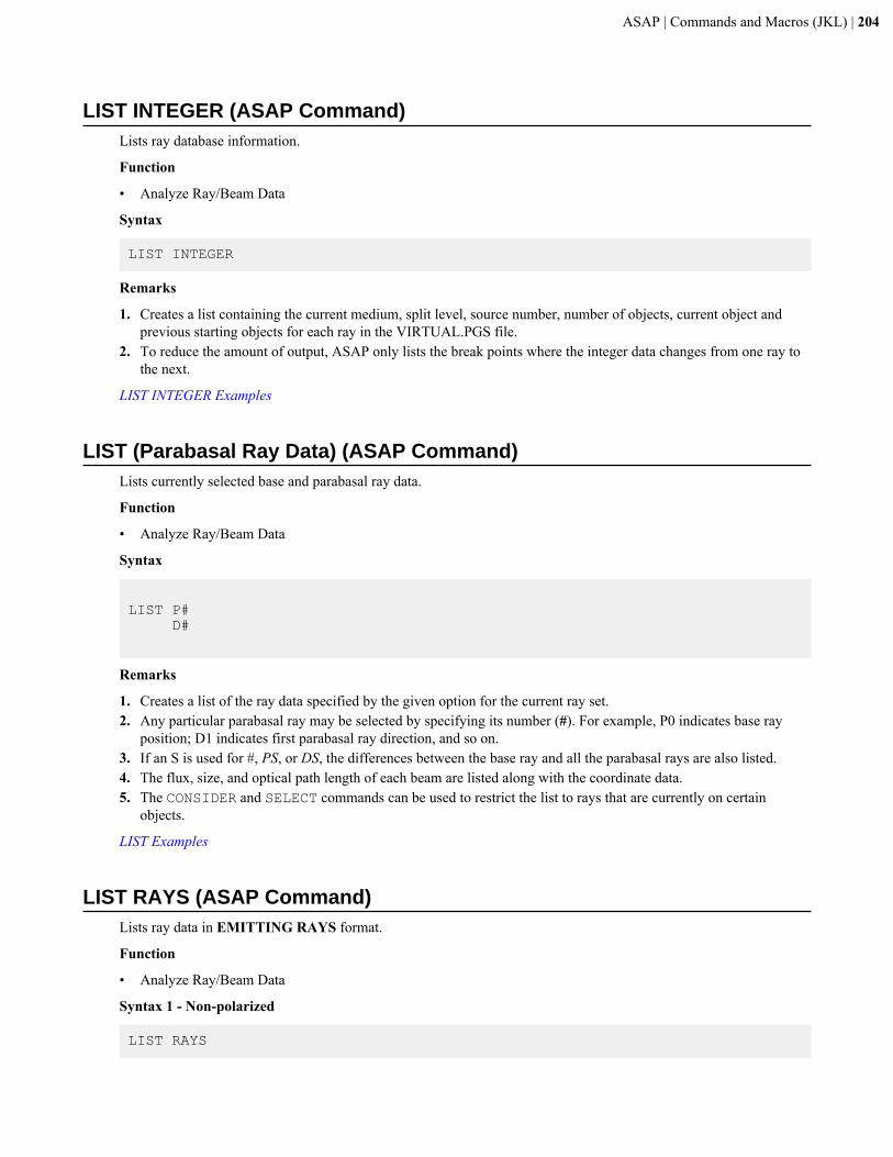
ASAP | Commands and Macros (JKL) | 204
LIST INTEGER (ASAP Command)Lists ray database information.
Function
• Analyze Ray/Beam Data
Syntax
LIST INTEGER
Remarks
1. Creates a list containing the current medium, split level, source number, number of objects, current object andprevious starting objects for each ray in the VIRTUAL.PGS file.
2. To reduce the amount of output, ASAP only lists the break points where the integer data changes from one ray tothe next.
LIST INTEGER Examples
LIST (Parabasal Ray Data) (ASAP Command)Lists currently selected base and parabasal ray data.
Function
• Analyze Ray/Beam Data
Syntax
LIST P# D#
Remarks
1. Creates a list of the ray data specified by the given option for the current ray set.2. Any particular parabasal ray may be selected by specifying its number (#). For example, P0 indicates base ray
position; D1 indicates first parabasal ray direction, and so on.3. If an S is used for #, PS, or DS, the differences between the base ray and all the parabasal rays are also listed.4. The flux, size, and optical path length of each beam are listed along with the coordinate data.5. The CONSIDER and SELECT commands can be used to restrict the list to rays that are currently on certain
objects.
LIST Examples
LIST RAYS (ASAP Command)Lists ray data in EMITTING RAYS format.
Function
• Analyze Ray/Beam Data
Syntax 1 - Non-polarized
LIST RAYS
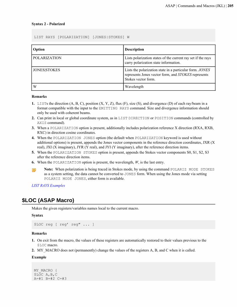
ASAP | Commands and Macros (JKL) | 205
Syntax 2 - Polarized
LIST RAYS [POLARIZATION] [JONES|STOKES] W
Option Description
POLARIZATION Lists polarization states of the current ray set if the rayscarry polarization state information.
JONES|STOKES Lists the polarization state in a particular form. JONESrepresents Jones vector form, and STOKES representsStokes vector form.
W Wavelength
Remarks
1. LISTs the direction (A, B, C), position (X, Y, Z), flux (F), size (S), and divergence (D) of each ray/beam in aformat compatible with the input to the EMITTING RAYS command. Size and divergence information shouldonly be used with coherent beams.
2. Can print in local or global coordinate system, as in LIST DIRECTION or POSITION commands (controlled byAXIS command).
3. When a POLARIZATION option is present, additionally includes polarization reference X direction (RXA, RXB,RXC) in direction cosine coordinates.
4. When the POLARIZATION JONES option (the default when POLARIZATION keyword is used withoutadditional options) is present, appends the Jones vector components in the reference direction coordinates, JXR (Xreal), JXI (X imaginary), JYR (Y real), and JYI (Y imaginary), after the reference direction items.
5. When the POLARIZATION STOKES option is present, appends the Stokes vector components S0, S1, S2, S3after the reference direction items.
6. When the POLARIZATION option is present, the wavelength, W, is the last entry.
Note: When polarization is being traced in Stokes mode, by using the command POLARIZ MODE STOKESas a system setting, the data cannot be converted to JONES form. When using the Jones mode via settingPOLARIZ MODE JONES, either form is available.
LIST RAYS Examples
$LOC (ASAP Macro)Makes the given registers/variables names local to the current macro.
Syntax
$LOC reg [ reg’ reg" ... ]
Remarks
1. On exit from the macro, the values of these registers are automatically restored to their values previous to the$LOC macro.
2. MY_MACRO does not (permanently) change the values of the registers A, B, and C when it is called.
Example
MY_MACRO {$LOC A,B,CA=#1 B=#2 C=#3
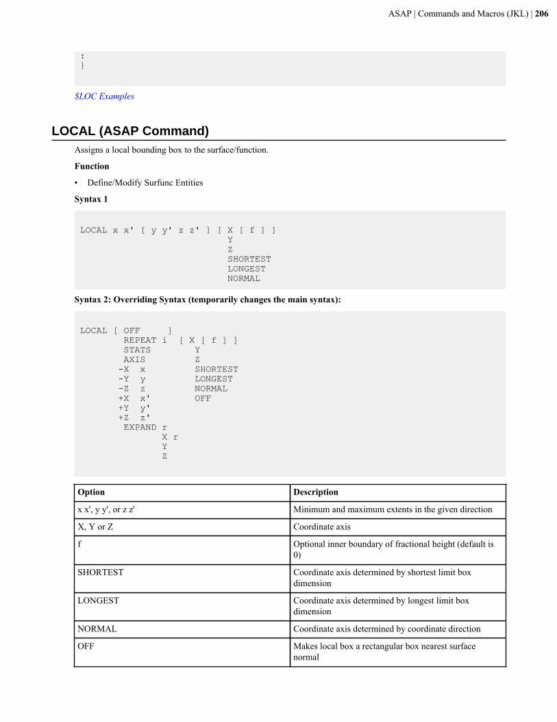
ASAP | Commands and Macros (JKL) | 206
:}
$LOC Examples
LOCAL (ASAP Command)Assigns a local bounding box to the surface/function.
Function
• Define/Modify Surfunc Entities
Syntax 1
LOCAL x x' [ y y' z z' ] [ X [ f ] ] Y Z SHORTEST LONGEST NORMAL
Syntax 2: Overriding Syntax (temporarily changes the main syntax):
LOCAL [ OFF ] REPEAT i [ X [ f ] ] STATS Y AXIS Z -X x SHORTEST -Y y LONGEST -Z z NORMAL +X x' OFF +Y y' +Z z' EXPAND r X r Y Z
Option Description
x x', y y', or z z' Minimum and maximum extents in the given direction
X, Y or Z Coordinate axis
f Optional inner boundary of fractional height (default is0)
SHORTEST Coordinate axis determined by shortest limit boxdimension
LONGEST Coordinate axis determined by longest limit boxdimension
NORMAL Coordinate axis determined by coordinate direction
OFF Makes local box a rectangular box nearest surfacenormal
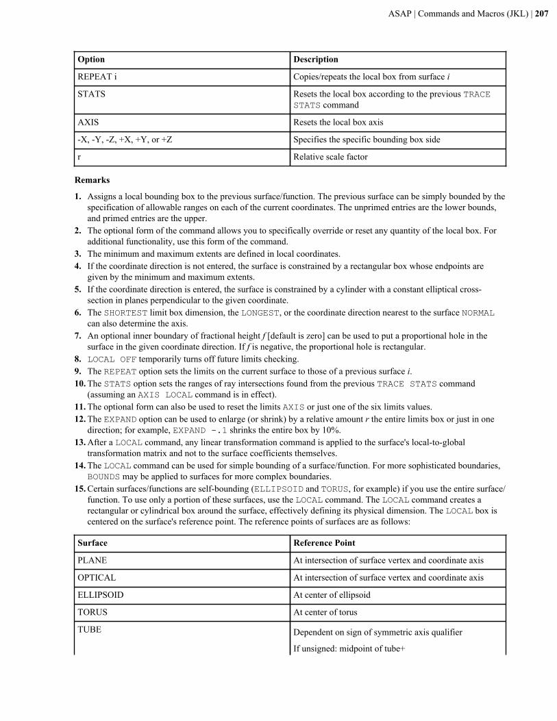
ASAP | Commands and Macros (JKL) | 207
Option Description
REPEAT i Copies/repeats the local box from surface i
STATS Resets the local box according to the previous TRACESTATS command
AXIS Resets the local box axis
-X, -Y, -Z, +X, +Y, or +Z Specifies the specific bounding box side
r Relative scale factor
Remarks
1. Assigns a local bounding box to the previous surface/function. The previous surface can be simply bounded by thespecification of allowable ranges on each of the current coordinates. The unprimed entries are the lower bounds,and primed entries are the upper.
2. The optional form of the command allows you to specifically override or reset any quantity of the local box. Foradditional functionality, use this form of the command.
3. The minimum and maximum extents are defined in local coordinates.4. If the coordinate direction is not entered, the surface is constrained by a rectangular box whose endpoints are
given by the minimum and maximum extents.5. If the coordinate direction is entered, the surface is constrained by a cylinder with a constant elliptical cross-
section in planes perpendicular to the given coordinate.6. The SHORTEST limit box dimension, the LONGEST, or the coordinate direction nearest to the surface NORMAL
can also determine the axis.7. An optional inner boundary of fractional height f [default is zero] can be used to put a proportional hole in the
surface in the given coordinate direction. If f is negative, the proportional hole is rectangular.8. LOCAL OFF temporarily turns off future limits checking.9. The REPEAT option sets the limits on the current surface to those of a previous surface i.10. The STATS option sets the ranges of ray intersections found from the previous TRACE STATS command
(assuming an AXIS LOCAL command is in effect).11. The optional form can also be used to reset the limits AXIS or just one of the six limits values.12. The EXPAND option can be used to enlarge (or shrink) by a relative amount r the entire limits box or just in one
direction; for example, EXPAND -.1 shrinks the entire box by 10%.13. After a LOCAL command, any linear transformation command is applied to the surface's local-to-global
transformation matrix and not to the surface coefficients themselves.14. The LOCAL command can be used for simple bounding of a surface/function. For more sophisticated boundaries,
BOUNDS may be applied to surfaces for more complex boundaries.15. Certain surfaces/functions are self-bounding (ELLIPSOID and TORUS, for example) if you use the entire surface/
function. To use only a portion of these surfaces, use the LOCAL command. The LOCAL command creates arectangular or cylindrical box around the surface, effectively defining its physical dimension. The LOCAL box iscentered on the surface's reference point. The reference points of surfaces are as follows:
Surface Reference Point
PLANE At intersection of surface vertex and coordinate axis
OPTICAL At intersection of surface vertex and coordinate axis
ELLIPSOID At center of ellipsoid
TORUS At center of torus
TUBE Dependent on sign of symmetric axis qualifier
If unsigned: midpoint of tube+
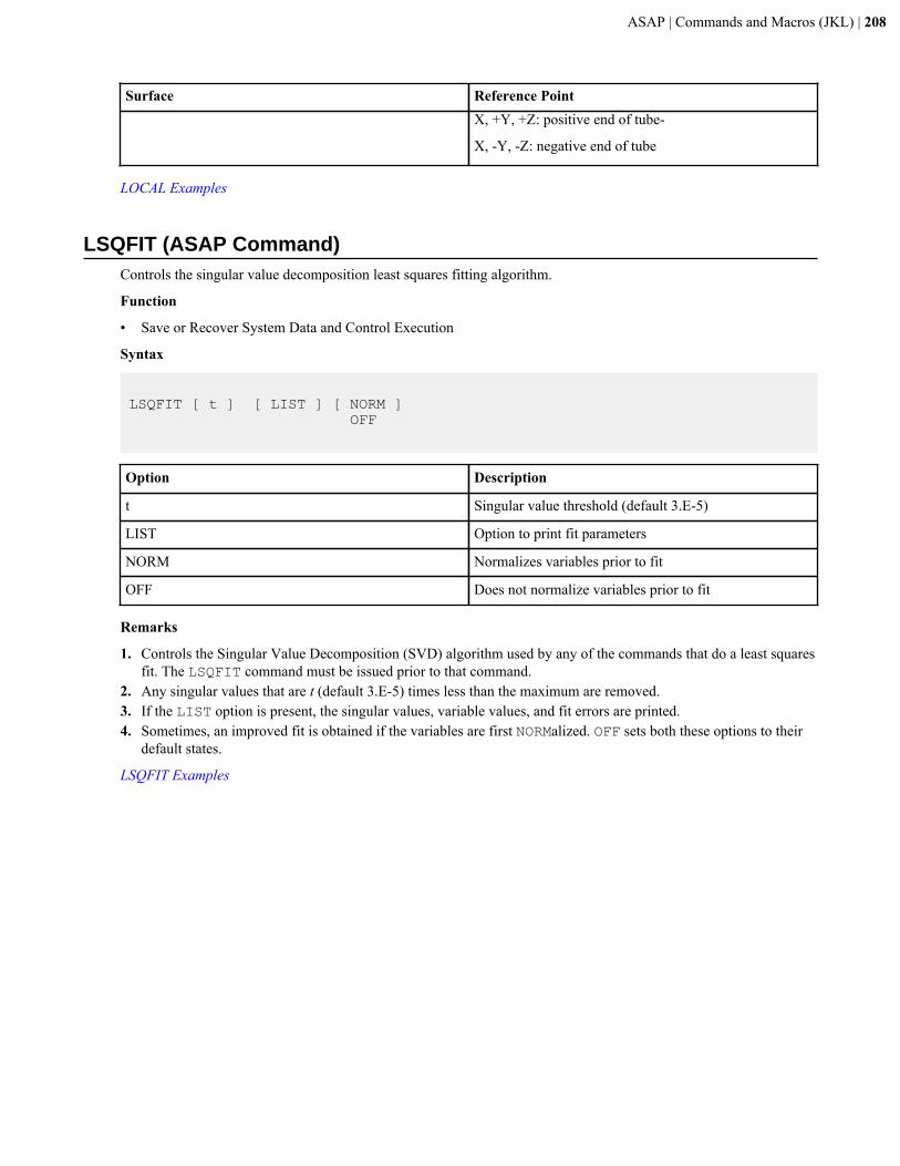
ASAP | Commands and Macros (JKL) | 208
Surface Reference PointX, +Y, +Z: positive end of tube-
X, -Y, -Z: negative end of tube
LOCAL Examples
LSQFIT (ASAP Command)Controls the singular value decomposition least squares fitting algorithm.
Function
• Save or Recover System Data and Control Execution
Syntax
LSQFIT [ t ] [ LIST ] [ NORM ] OFF
Option Description
t Singular value threshold (default 3.E-5)
LIST Option to print fit parameters
NORM Normalizes variables prior to fit
OFF Does not normalize variables prior to fit
Remarks
1. Controls the Singular Value Decomposition (SVD) algorithm used by any of the commands that do a least squaresfit. The LSQFIT command must be issued prior to that command.
2. Any singular values that are t (default 3.E-5) times less than the maximum are removed.3. If the LIST option is present, the singular values, variable values, and fit errors are printed.4. Sometimes, an improved fit is obtained if the variables are first NORMalized. OFF sets both these options to their
default states.
LSQFIT Examples

ASAP | Commands and Macros (M) | 209
Commands and Macros (M)
Topics in this section of the Contents tab include ASAP commands and macros that begin with the letter “M”.
MANGIN (ASAP Command)Creates a Mangin mirror.
Function
• Define/Modify Lens Entities
Syntax
MANGIN X x t h m [ RD r r' ] Y y CV c c' Z z FL f b [ a ] a APLANAT
Option Description
X Y or Z Global coordinate axis
x y or z Location on the global coordinate axis
t Lens thickness
h Aperture height
m Internal medium (number or name)
f Focal length
b Bending parameter
c c' Curvatures of the two surfaces
r r' Radii of curvature of the two surfaces
RD Surfaces defined by radius values
CV Surfaces defined by curvature values
FL Surfaces defined by focal length and bending parameter
APLANAT Bending factor and one conic constant are automaticallycalculated
a Conjugate factor
Remarks
1. A Mangin mirror is a lens with a reflective second conicoid; rays are refracted twice at the first conicoid.2. The format of this command is identical to that of the SINGLET, except that the second surface is reflective; that
is, rays are refracted twice at the first surface. The following remarks are the same for the SINGLET.3. This lens entity starts out normal to the defined global coordinate axis (X, Y or Z).4. RD is used to specify radii of curvature (r r'), CV is used to specify curvatures (c c'), and FL is used to specify
focal length f and bending parameter b.
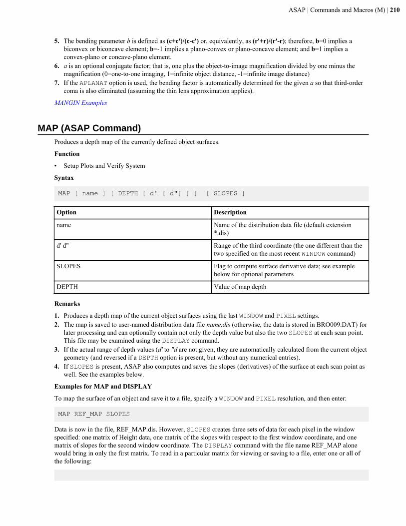
ASAP | Commands and Macros (M) | 210
5. The bending parameter b is defined as (c+c')/(c-c') or, equivalently, as (r'+r)/(r'-r); therefore, b=0 implies abiconvex or biconcave element; b=-1 implies a plano-convex or plano-concave element; and b=1 implies aconvex-plano or concave-plano element.
6. a is an optional conjugate factor; that is, one plus the object-to-image magnification divided by one minus themagnification (0=one-to-one imaging, 1=infinite object distance, -1=infinite image distance)
7. If the APLANAT option is used, the bending factor is automatically determined for the given a so that third-ordercoma is also eliminated (assuming the thin lens approximation applies).
MANGIN Examples
MAP (ASAP Command)Produces a depth map of the currently defined object surfaces.
Function
• Setup Plots and Verify System
Syntax
MAP [ name ] [ DEPTH [ d' [ d"] ] ] [ SLOPES ]
Option Description
name Name of the distribution data file (default extension*.dis)
d' d" Range of the third coordinate (the one different than thetwo specified on the most recent WINDOW command)
SLOPES Flag to compute surface derivative data; see examplebelow for optional parameters
DEPTH Value of map depth
Remarks
1. Produces a depth map of the current object surfaces using the last WINDOW and PIXEL settings.2. The map is saved to user-named distribution data file name.dis (otherwise, the data is stored in BRO009.DAT) for
later processing and can optionally contain not only the depth value but also the two SLOPES at each scan point.This file may be examined using the DISPLAY command.
3. If the actual range of depth values (d' to "d are not given, they are automatically calculated from the current objectgeometry (and reversed if a DEPTH option is present, but without any numerical entries).
4. If SLOPES is present, ASAP also computes and saves the slopes (derivatives) of the surface at each scan point aswell. See the examples below.
Examples for MAP and DISPLAY
To map the surface of an object and save it to a file, specify a WINDOW and PIXEL resolution, and then enter:
MAP REF_MAP SLOPES
Data is now in the file, REF_MAP.dis. However, SLOPES creates three sets of data for each pixel in the windowspecified: one matrix of Height data, one matrix of the slopes with respect to the first window coordinate, and onematrix of slopes for the second window coordinate. The DISPLAY command with the file name REF_MAP alonewould bring in only the first matrix. To read in a particular matrix for viewing or saving to a file, enter one or all ofthe following:
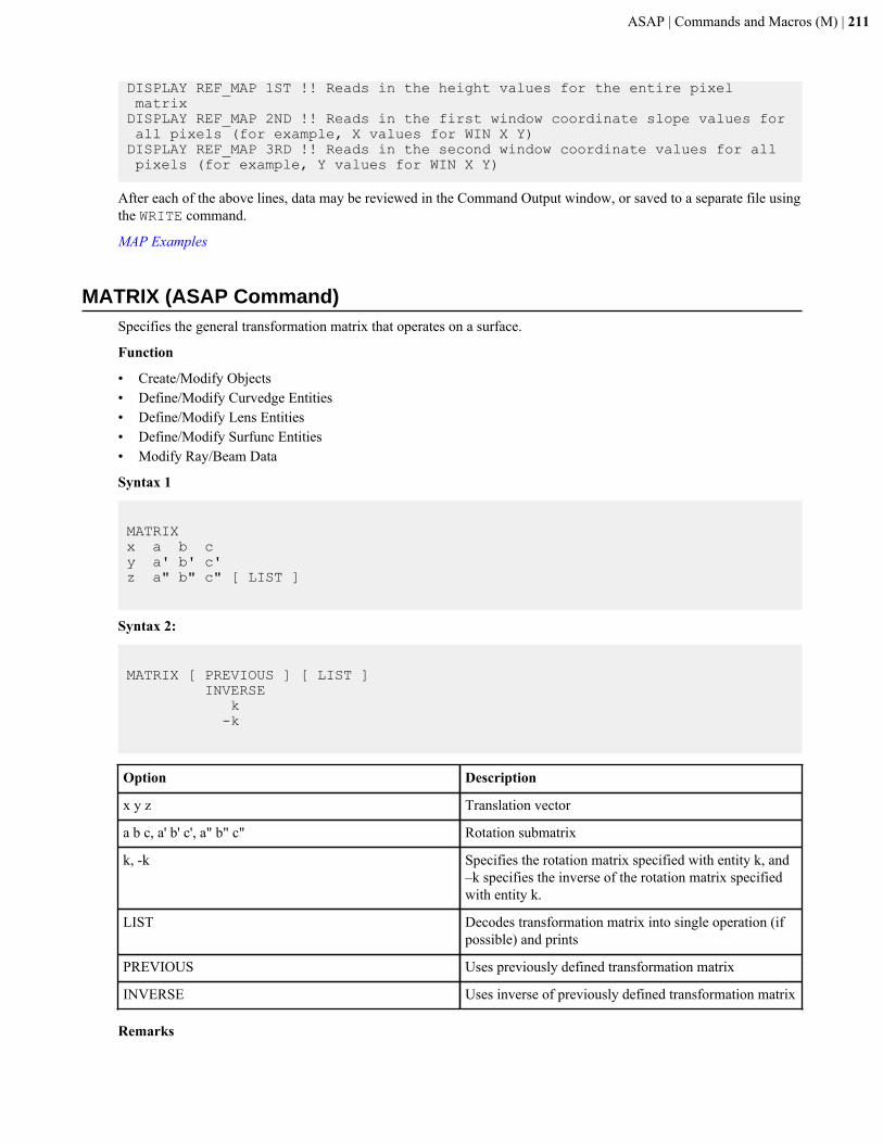
ASAP | Commands and Macros (M) | 211
DISPLAY REF_MAP 1ST !! Reads in the height values for the entire pixel matrixDISPLAY REF_MAP 2ND !! Reads in the first window coordinate slope values for all pixels (for example, X values for WIN X Y)DISPLAY REF_MAP 3RD !! Reads in the second window coordinate values for all pixels (for example, Y values for WIN X Y)
After each of the above lines, data may be reviewed in the Command Output window, or saved to a separate file usingthe WRITE command.
MAP Examples
MATRIX (ASAP Command)Specifies the general transformation matrix that operates on a surface.
Function
• Create/Modify Objects• Define/Modify Curvedge Entities• Define/Modify Lens Entities• Define/Modify Surfunc Entities• Modify Ray/Beam Data
Syntax 1
MATRIXx a b cy a' b' c'z a" b" c" [ LIST ]
Syntax 2:
MATRIX [ PREVIOUS ] [ LIST ] INVERSE k -k
Option Description
x y z Translation vector
a b c, a' b' c', a" b" c" Rotation submatrix
k, -k Specifies the rotation matrix specified with entity k, and–k specifies the inverse of the rotation matrix specifiedwith entity k.
LIST Decodes transformation matrix into single operation (ifpossible) and prints
PREVIOUS Uses previously defined transformation matrix
INVERSE Uses inverse of previously defined transformation matrix
Remarks
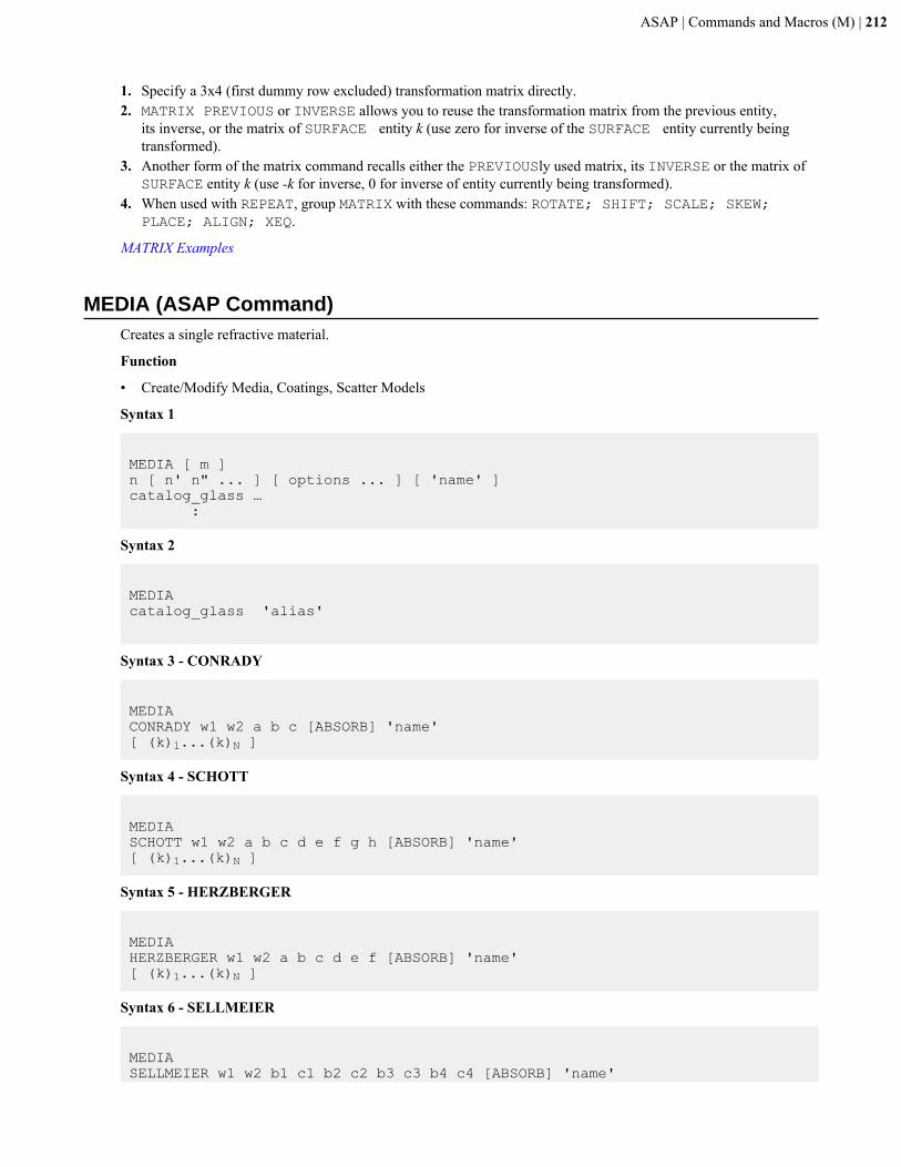
ASAP | Commands and Macros (M) | 212
1. Specify a 3x4 (first dummy row excluded) transformation matrix directly.2. MATRIX PREVIOUS or INVERSE allows you to reuse the transformation matrix from the previous entity,
its inverse, or the matrix of SURFACE entity k (use zero for inverse of the SURFACE entity currently beingtransformed).
3. Another form of the matrix command recalls either the PREVIOUSly used matrix, its INVERSE or the matrix ofSURFACE entity k (use -k for inverse, 0 for inverse of entity currently being transformed).
4. When used with REPEAT, group MATRIX with these commands: ROTATE; SHIFT; SCALE; SKEW;PLACE; ALIGN; XEQ.
MATRIX Examples
MEDIA (ASAP Command)Creates a single refractive material.
Function
• Create/Modify Media, Coatings, Scatter Models
Syntax 1
MEDIA [ m ] n [ n' n" ... ] [ options ... ] [ 'name' ]catalog_glass … :
Syntax 2
MEDIAcatalog_glass 'alias'
Syntax 3 - CONRADY
MEDIA CONRADY w1 w2 a b c [ABSORB] 'name'[ (k)1...(k)N ]
Syntax 4 - SCHOTT
MEDIA SCHOTT w1 w2 a b c d e f g h [ABSORB] 'name'[ (k)1...(k)N ]
Syntax 5 - HERZBERGER
MEDIA HERZBERGER w1 w2 a b c d e f [ABSORB] 'name'[ (k)1...(k)N ]
Syntax 6 - SELLMEIER
MEDIA SELLMEIER w1 w2 b1 c1 b2 c2 b3 c3 b4 c4 [ABSORB] 'name'
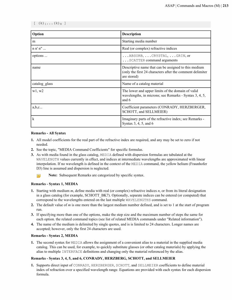
ASAP | Commands and Macros (M) | 213
[ (k)1...(k)N ]
Option Description
m Starting media number
n n' n" ... Real (or complex) refractive indices
options ... ...ABSORB, ...CRYSTAL, ...GRIN, or...SCATTER command arguments
name Descriptive name that can be assigned to this medium(only the first 24 characters after the comment delimiterare stored)
catalog_glass Name of a catalog material
w1, w2 The lower and upper limits of the domain of validwavelengths, in microns; see Remarks - Syntax 3, 4, 5,and 6
a,b,c... Coefficient parameters (CONRADY, HERZBERGER,SCHOTT, and SELLMEIER)
k Imaginary parts of the refractive index; see Remarks -Syntax 3, 4, 5, and 6
Remarks - All Syntax
1. All model coefficients for the real part of the refractive index are required, and any may be set to zero if notneeded.
2. See the topic, "MEDIA Command Coefficients" for specific formulas.3. As with media found in the glass catalog, MEDIA defined with dispersion formulas are tabulated at the
WAVELENGTH values currently in effect, and indices at intermediate wavelengths are approximated with linearinterpolation. If no wavelength is defined in the context of the MEDIA command, the yellow helium (FraunhoferD3) line is assumed and dispersion is neglected.
Note: Subsequent Remarks are categorized by specific syntax.
Remarks - Syntax 1, MEDIA
1. Starting with medium m, define media with real (or complex) refractive indices n, or from its literal designationin a glass catalog (for example, SCHOTT_BK7). Optionally, separate indices can be entered (or computed) thatcorrespond to the wavelengths entered on the last multiple WAVELENGTHS command.
2. The default value of m is one more than the largest medium number defined, and is set to 1 at the start of programrun.
3. If specifying more than one of the options, make the step size and the maximum number of steps the same foreach option. the related command topics (see list of related MEDIA commands under "Related information").
4. The name of the medium is delimited by single quotes, and is is limited to 24 characters. Longer names areaccepted; however, only the first 24 characters are used.
Remarks - Syntax 2, MEDIA
1. The second syntax for MEDIA allows the assignment of a convenient alias to a material in the supplied mediacatalog. This can be used, for example, to quickly substitute glasses (or other catalog materials) by applying thealias to multiple INTERFACE definitions and changing only the material referenced by the alias.
Remarks - Syntax 3, 4, 5, and 6, CONRADY, HERZBERG, SCHOTT, and SELLMEIER
1. Supports direct input of CONRADY, HERZBERGER, SCHOTT, and SELLMEIER coefficients to define materialindex of refraction over a specified wavelength range. Equations are provided with each syntax for each dispersionformula.
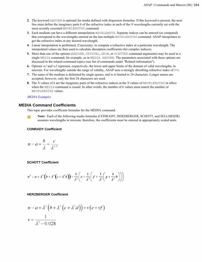
ASAP | Commands and Macros (M) | 214
2. The keyword ABSORB is optional for media defined with dispersion formulae. If this keyword is present, the nextline must define the imaginary parts k of the refractive index at each of the N wavelengths currently set with themost recently executed WAVELENGTHS command.
3. Each medium can have a different interpolation WAVELENGTH. Separate indices can be entered (or computed)that correspond to the wavelengths entered on the last multiple WAVELENGTHS command. ASAP interpolates toget the refractive index at any desired wavelength.
4. Linear interpolation is performed, if necessary, to compute a refractive index at a particular wavelength. Theinterpolated values are then used to calculate absorption coefficients (for complex indices).
5. More than one of the options (ABSORB, CRYSTAL, GRIN, or SCATTER command arguments) may be used in asingle MEDIA command; for example, as in MEDIA ABSORB. The parameters associated with these options arediscussed in the related command topics (see list of commands under "Related information").
6. Options w1 and w2 represent, respectively, the lower and upper limits of the domain of valid wavelengths, inmicrons. For wavelengths outside the range of validity, ASAP uses a strongly absorbing refractive index of 1+i.
7. The name of the medium is delimited by single quotes, and is is limited to 24 characters. Longer names areaccepted; however, only the first 24 characters are used.
8. The N values of k are the imaginary parts of the refractive indices at the N values of WAVELENGTHS in effectwhen the MEDIA command is issued. In other words, the number of k values must match the number ofWAVELENGTHS values.
MEDIA Examples
MEDIA Command CoefficientsThis topic provides coefficient formulas for the MEDIA command.
Note: Each of the following media formulas (CONRADY, HERZBERGER, SCHOTT, and SELLMEIER)assumes wavelengths in microns; therefore, the coefficients must be entered in appropriately scaled units.
CONRADY Coefficient
SCHOTT Coefficient
HERZBERGER Coefficient
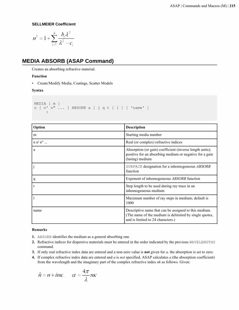
ASAP | Commands and Macros (M) | 215
SELLMEIER Coefficient
MEDIA ABSORB (ASAP Command)Creates an absorbing refractive material.
Function
• Create/Modify Media, Coatings, Scatter Models
Syntax
MEDIA [ m ]n [ n' n" ... ] ABSORB a [ j q t [ l ] [ 'name' ] :
Option Description
m Starting media number
n n' n" ... Real (or complex) refractive indices
a Absorption (or gain) coefficient (inverse length units);positive for an absorbing medium or negative for a gain(lasing) medium
j SURFACE designation for a inhomogeneous ABSORBfunction
q Exponent of inhomogeneous ABSORB function
t Step length to be used during ray trace in aninhomogeneous medium
l Maximum number of ray steps in medium; default is1000
name Descriptive name that can be assigned to this medium.(The name of the medium is delimited by single quotes,and is limited to 24 characters.)
Remarks
1. ABSORB identifies the medium as a general absorbing one.2. Refractive indices for dispersive materials must be entered in the order indicated by the previous WAVELENGTHS
command.3. If only real refractive index data are entered and a non-zero value is not given for a, the absorption is set to zero.4. If complex refractive index data are entered and a is not specified, ASAP calculates a (the absorption coefficient)
from the wavelength and the imaginary part of the complex refractive index nk as follows. Given:
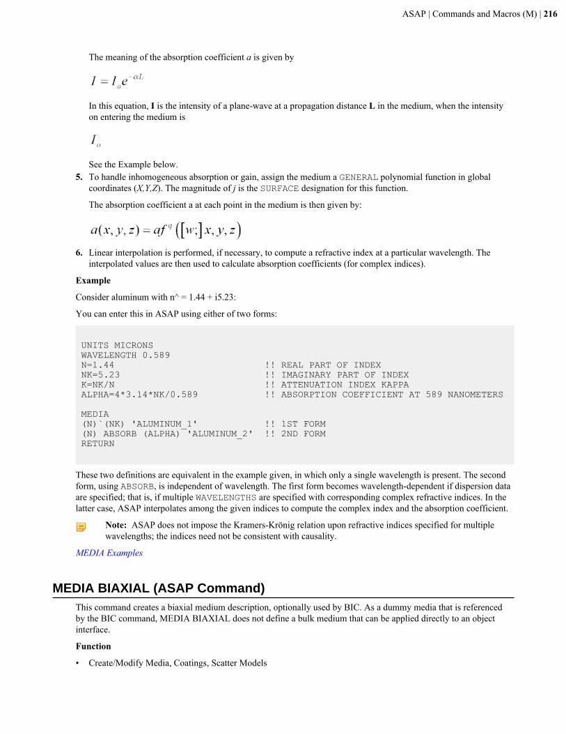
ASAP | Commands and Macros (M) | 216
The meaning of the absorption coefficient a is given by
In this equation, I is the intensity of a plane-wave at a propagation distance L in the medium, when the intensityon entering the medium is
See the Example below.5. To handle inhomogeneous absorption or gain, assign the medium a GENERAL polynomial function in global
coordinates (X,Y,Z). The magnitude of j is the SURFACE designation for this function.
The absorption coefficient a at each point in the medium is then given by:
6. Linear interpolation is performed, if necessary, to compute a refractive index at a particular wavelength. Theinterpolated values are then used to calculate absorption coefficients (for complex indices).
Example
Consider aluminum with n^ = 1.44 + i5.23:
You can enter this in ASAP using either of two forms:
UNITS MICRONSWAVELENGTH 0.589N=1.44 !! REAL PART OF INDEXNK=5.23 !! IMAGINARY PART OF INDEXK=NK/N !! ATTENUATION INDEX KAPPAALPHA=4*3.14*NK/0.589 !! ABSORPTION COEFFICIENT AT 589 NANOMETERS
MEDIA(N)`(NK) 'ALUMINUM_1' !! 1ST FORM(N) ABSORB (ALPHA) 'ALUMINUM_2' !! 2ND FORMRETURN
These two definitions are equivalent in the example given, in which only a single wavelength is present. The secondform, using ABSORB, is independent of wavelength. The first form becomes wavelength-dependent if dispersion dataare specified; that is, if multiple WAVELENGTHS are specified with corresponding complex refractive indices. In thelatter case, ASAP interpolates among the given indices to compute the complex index and the absorption coefficient.
Note: ASAP does not impose the Kramers-Krönig relation upon refractive indices specified for multiplewavelengths; the indices need not be consistent with causality.
MEDIA Examples
MEDIA BIAXIAL (ASAP Command)This command creates a biaxial medium description, optionally used by BIC. As a dummy media that is referencedby the BIC command, MEDIA BIAXIAL does not define a bulk medium that can be applied directly to an objectinterface.
Function
• Create/Modify Media, Coatings, Scatter Models
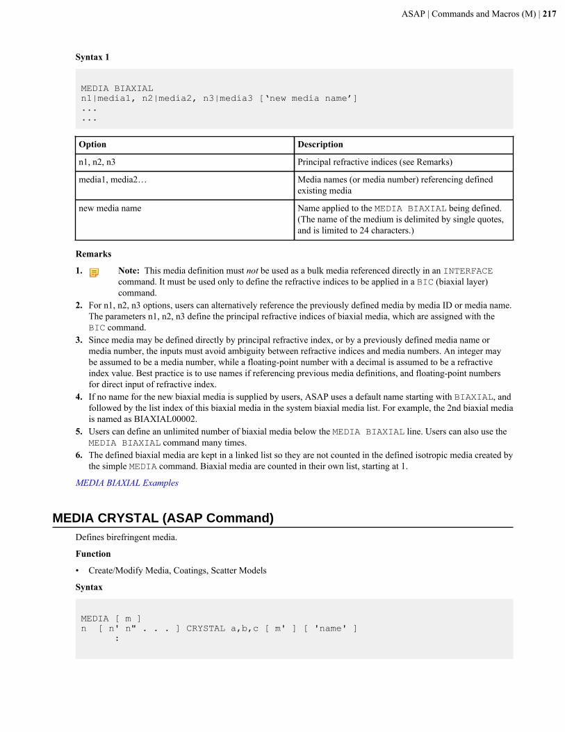
ASAP | Commands and Macros (M) | 217
Syntax 1
MEDIA BIAXIALn1|media1, n2|media2, n3|media3 [‘new media name’]......
Option Description
n1, n2, n3 Principal refractive indices (see Remarks)
media1, media2… Media names (or media number) referencing definedexisting media
new media name Name applied to the MEDIA BIAXIAL being defined.(The name of the medium is delimited by single quotes,and is limited to 24 characters.)
Remarks
1. Note: This media definition must not be used as a bulk media referenced directly in an INTERFACEcommand. It must be used only to define the refractive indices to be applied in a BIC (biaxial layer)command.
2. For n1, n2, n3 options, users can alternatively reference the previously defined media by media ID or media name.The parameters n1, n2, n3 define the principal refractive indices of biaxial media, which are assigned with theBIC command.
3. Since media may be defined directly by principal refractive index, or by a previously defined media name ormedia number, the inputs must avoid ambiguity between refractive indices and media numbers. An integer maybe assumed to be a media number, while a floating-point number with a decimal is assumed to be a refractiveindex value. Best practice is to use names if referencing previous media definitions, and floating-point numbersfor direct input of refractive index.
4. If no name for the new biaxial media is supplied by users, ASAP uses a default name starting with BIAXIAL, andfollowed by the list index of this biaxial media in the system biaxial media list. For example, the 2nd biaxial mediais named as BIAXIAL00002.
5. Users can define an unlimited number of biaxial media below the MEDIA BIAXIAL line. Users can also use theMEDIA BIAXIAL command many times.
6. The defined biaxial media are kept in a linked list so they are not counted in the defined isotropic media created bythe simple MEDIA command. Biaxial media are counted in their own list, starting at 1.
MEDIA BIAXIAL Examples
MEDIA CRYSTAL (ASAP Command)Defines birefringent media.
Function
• Create/Modify Media, Coatings, Scatter Models
Syntax
MEDIA [ m ]n [ n' n" . . . ] CRYSTAL a,b,c [ m' ] [ 'name' ] :
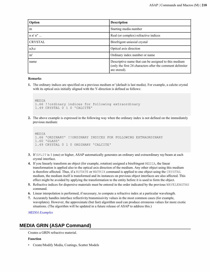
ASAP | Commands and Macros (M) | 218
Option Description
m Starting media number
n n' n" ... Real (or complex) refractive indices
CRYSTAL Birefrigent uniaxial crystal
a,b,c Optical axis direction
m' Ordinary index number or name
name Descriptive name that can be assigned to this medium(only the first 24 characters after the comment delimiterare stored).
Remarks
1. The ordinary indices are specified on a previous medium m' (default is last media). For example, a calcite crystalwith its optical axis initially aligned with the Y-direction is defined as follows:
MEDIA1.66 !!ordinary indices for following extraordinary1.49 CRYSTAL 0 1 0 'CALCITE'
2. The above example is expressed in the following way when the ordinary index is not defined on the immediatelyprevious medium:
MEDIA1.66 'ORDINARY' !!ORDINARY INDICES FOR FOLLOWING EXTRAORDINARY1.60 'GLASS'1.49 CRYSTAL 0 1 0 ORDINARY 'CALCITE'
3. If SPLIT is 1 (one) or higher, ASAP automatically generates an ordinary and extraordinary ray/beam at eachcrystal interface.
4. If you linearly transform an object (for example, rotation) assigned a birefringent MEDIA, the lineartransformation is applied also to the optical axis direction of the medium. Any other object using this mediumis therefore affected. Thus, if a ROTATE or MATRIX command is applied to one object using the CRYSTALmedium, the medium itself is transformed and its instances on previous object interfaces are also affected. Thiseffect might be avoided by applying the transformation to the entity before it is used to form the object.
5. Refractive indices for dispersive materials must be entered in the order indicated by the previous WAVELENGTHScommand.
6. Linear interpolation is performed, if necessary, to compute a refractive index at a particular wavelength.7. Accurately handles interface reflectivity/transmissivity values in the most common cases (for example,
waveplates). However, the approximate (but fast) algorithm used can produce erroneous values for more exoticsituations. (The algorithm will be updated in a future release of ASAP to address this.)
MEDIA Examples
MEDIA GRIN (ASAP Command)Creates a GRIN refractive material.
Function
• Create/Modify Media, Coatings, Scatter Models
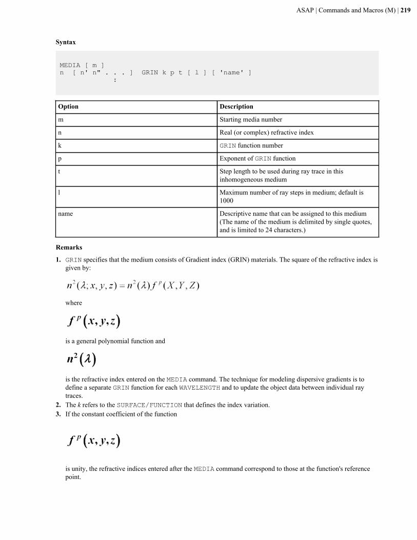
ASAP | Commands and Macros (M) | 219
Syntax
MEDIA [ m ]n [ n' n" . . . ] GRIN k p t [ l ] [ 'name' ] :
Option Description
m Starting media number
n Real (or complex) refractive index
k GRIN function number
p Exponent of GRIN function
t Step length to be used during ray trace in thisinhomogeneous medium
l Maximum number of ray steps in medium; default is1000
name Descriptive name that can be assigned to this medium(The name of the medium is delimited by single quotes,and is limited to 24 characters.)
Remarks
1. GRIN specifies that the medium consists of Gradient index (GRIN) materials. The square of the refractive index isgiven by:
where
is a general polynomial function and
is the refractive index entered on the MEDIA command. The technique for modeling dispersive gradients is todefine a separate GRIN function for each WAVELENGTH and to update the object data between individual raytraces.
2. The k refers to the SURFACE/FUNCTION that defines the index variation.3. If the constant coefficient of the function
is unity, the refractive indices entered after the MEDIA command correspond to those at the function's referencepoint.

ASAP | Commands and Macros (M) | 220
4. The GRIN function is defined in global coordinates. This is of little consequence if the gradients are radial (thereis no position dependence along the axis), but if the desired gradient is axial, you may have to SHIFT the gradientto the correct global coordinates to align the gradient with the object.
5. The function can be ARRAYed.6. You may need to adjust the HALT and/or CUTOFF values to account for step length and maximum number of ray
steps.
MEDIA Examples
MEDIA SCATTER (ASAP Command)Assigns to medium a GENERAL polynomial or USERFUNC function in the global coordinates X, Y, Z.
Function
• Create/Modify Media, Coatings, Scatter Models
Syntax
MEDIA [ i ]n [ n' n" . . . ] SCATTER m [ k e t [ l ] ] 'name' :
Option Description
i Starting media number
SCATTER Allows specification of the maximum number ofscattering events per ray for all volumetric models,including homogeneous models expressed by the shortform. The maximum number of scattering events per raydefaults to 1000 if l is not specified.
m Refers to a VOLUME scattering MODEL
k Its magnitude is the SURFACE designation for thisfunction
e Exponent of the scattering function
t Step length used for tracing a ray when tracing a ray inthis inhomogeneous medium
l Maximum number of ray steps in medium
name Descriptive name that can be assigned to this medium(The name of the medium is delimited by single quotes,and is limited to 24 characters.)
Remarks
1. The medium is homogeneously scattering by default.2. The medium is inhomogeneously scattering if a SURFACE k is specified, which has the effect of multiplying the
homogeneous scattering model m by the modified SURFACE function.
3. The SURFACE function k, if specified, must be greater than zero at all points in regions characterized by mediumi.
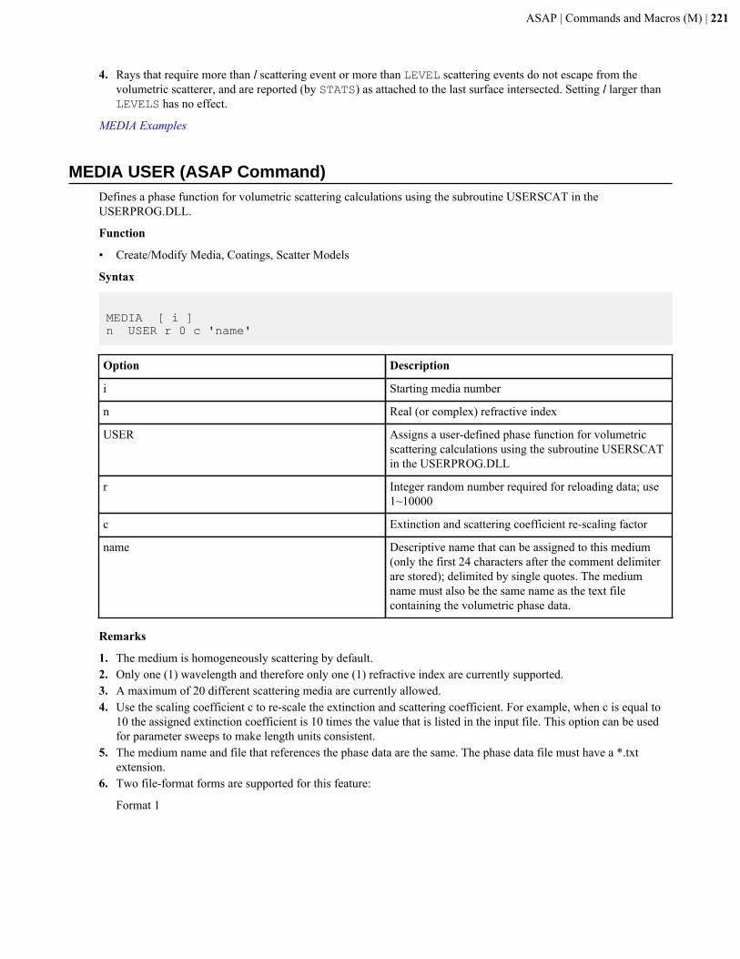
ASAP | Commands and Macros (M) | 221
4. Rays that require more than l scattering event or more than LEVEL scattering events do not escape from thevolumetric scatterer, and are reported (by STATS) as attached to the last surface intersected. Setting l larger thanLEVELS has no effect.
MEDIA Examples
MEDIA USER (ASAP Command)Defines a phase function for volumetric scattering calculations using the subroutine USERSCAT in theUSERPROG.DLL.
Function
• Create/Modify Media, Coatings, Scatter Models
Syntax
MEDIA [ i ]n USER r 0 c 'name'
Option Description
i Starting media number
n Real (or complex) refractive index
USER Assigns a user-defined phase function for volumetricscattering calculations using the subroutine USERSCATin the USERPROG.DLL
r Integer random number required for reloading data; use1~10000
c Extinction and scattering coefficient re-scaling factor
name Descriptive name that can be assigned to this medium(only the first 24 characters after the comment delimiterare stored); delimited by single quotes. The mediumname must also be the same name as the text filecontaining the volumetric phase data.
Remarks
1. The medium is homogeneously scattering by default.2. Only one (1) wavelength and therefore only one (1) refractive index are currently supported.3. A maximum of 20 different scattering media are currently allowed.4. Use the scaling coefficient c to re-scale the extinction and scattering coefficient. For example, when c is equal to
10 the assigned extinction coefficient is 10 times the value that is listed in the input file. This option can be usedfor parameter sweeps to make length units consistent.
5. The medium name and file that references the phase data are the same. The phase data file must have a *.txtextension.
6. Two file-format forms are supported for this feature:
Format 1
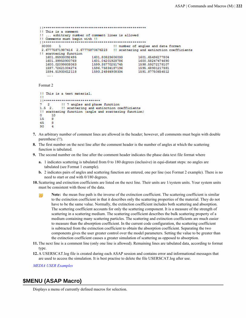
ASAP | Commands and Macros (M) | 222
Format 2
7. An arbitrary number of comment lines are allowed in the header; however, all comments must begin with doubleparenthese (!!).
8. The first number on the next line after the comment header is the number of angles at which the scatteringfunction is tabulated.
9. The second number on the line after the comment header indicates the phase data text file format where
a. 1 indicates scattering is tabulated from 0 to 180 degrees (inclusive) in equi-distant steps: no angles aretabulated (see Format 1 example).
b. 2 indicates pairs of angles and scattering function are entered, one per line (see Format 2 example). There is noneed to start or end with 0/180 degrees.
10. Scattering and extinction coefficients are listed on the next line. Their units are 1/system units. Your system unitsmust be consistent with those of the data.
Note: the mean free path is the inverse of the extinction coefficient. The scattering coefficient is similarto the extinction coefficient in that it describes only the scattering properties of the material. They do nothave to be the same value. Normally, the extinction coefficient includes both scattering and absorption.The scattering coefficient accounts for only the scattering component. It is a measure of the strength ofscattering in a scattering medium. The scattering coefficient describes the bulk scattering property of amedium containing many scattering particles. The scattering and extinction coefficients are much easierto measure than the absorption coefficient. In the current code configuration, the scattering coefficientis subtracted from the extinction coefficient to obtain the absorption coefficient. Separating the twocomponents gives the user greater control over the model parameters. Setting the value to be greater thanthe extinction coefficient causes a greater simulation of scattering as opposed to absorption.
11. The next line is a comment line (only one line is allowed). Remaining lines are tabulated data, according to formattype.
12. A USERSCAT.log file is created during each ASAP session and contains error and informational messages thatare used to access the simulation. It is best practise to delete the file USERSCAT.log after use.
MEDIA USER Examples
$MENU (ASAP Macro)Displays a menu of currently defined macros for selection.
ASAP | Commands and Macros (M) | 223
Syntax
$MENU [ m ] [ 'title' ]&MENU
Remarks
1. Displays a menu of current macro library names (and any descriptions found on the definition line). Make aselection by selecting the name of the desired macro and clicking OK.
2. The menu entries are displayed horizontally in columns by default. The m is the maximum number of columns touse (default 6). For example, entering a 1 would force the menu entries into one vertical column.
$MENU Examples
MESH (ASAP Command)Creates a 3D representation of the distribution in the system vector (*.VCR) file.
Function
• Display/Modify Data Distributions
Syntax
MESH [ i [ j ] ] [ LOW ] HIGH
Option Description
i Line across specification
j Line down specification
Remarks
1. Writes a three-dimensional representation (wireframe or LOW / HIGH-resolution shaded "surfaces") of thedistribution into the 3D system vector file so that it can be REPLOTted with other geometrical entities.
2. If given, only every ith line across or jth line down is written (defaults are 1).
MESH Examples
MICROSTRUCTURE (ASAP Command)Creates a replicated microstructure scattering geometry/object.
Function
• Define/Modify Entities or Single Entity Objects• Define/Modify Surface/Function Entities• Object Creation
Syntax 1
MICROSTRUCTURE X e j1 j2 j3 … [ SCALE SFAC ] [ PITCH PITFUNCX PITFUNCY ]
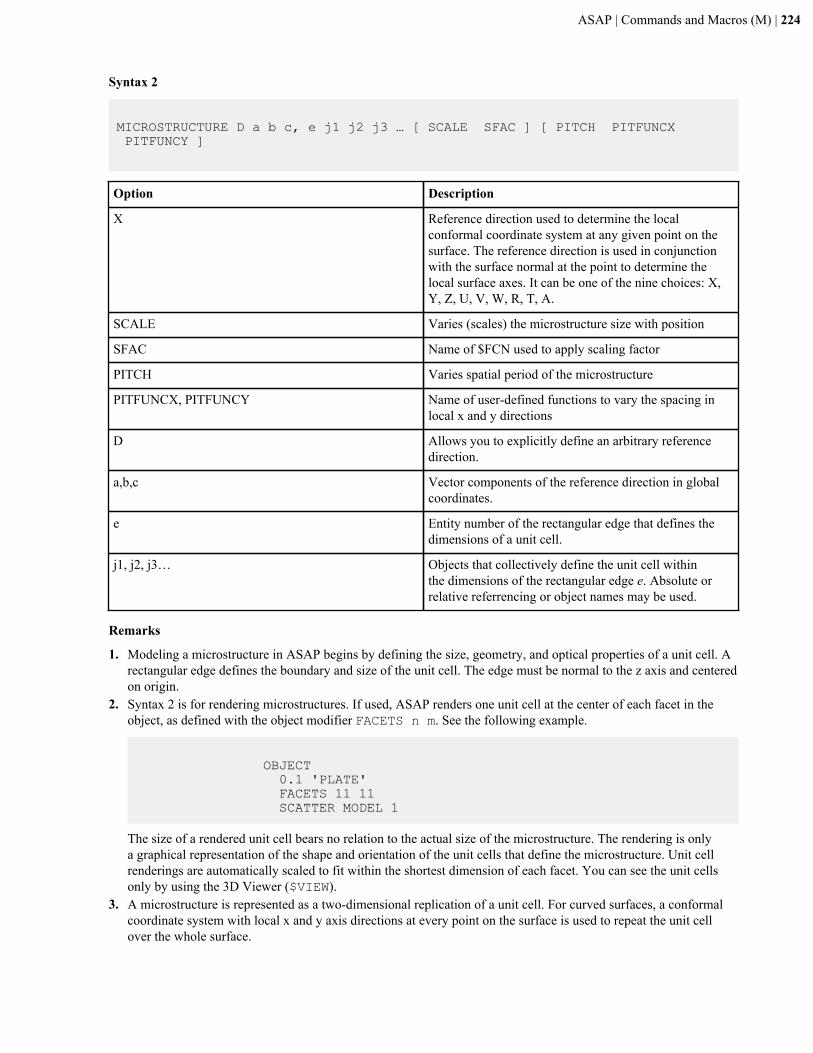
ASAP | Commands and Macros (M) | 224
Syntax 2
MICROSTRUCTURE D a b c, e j1 j2 j3 … [ SCALE SFAC ] [ PITCH PITFUNCX PITFUNCY ]
Option Description
X Reference direction used to determine the localconformal coordinate system at any given point on thesurface. The reference direction is used in conjunctionwith the surface normal at the point to determine thelocal surface axes. It can be one of the nine choices: X,Y, Z, U, V, W, R, T, A.
SCALE Varies (scales) the microstructure size with position
SFAC Name of $FCN used to apply scaling factor
PITCH Varies spatial period of the microstructure
PITFUNCX, PITFUNCY Name of user-defined functions to vary the spacing inlocal x and y directions
D Allows you to explicitly define an arbitrary referencedirection.
a,b,c Vector components of the reference direction in globalcoordinates.
e Entity number of the rectangular edge that defines thedimensions of a unit cell.
j1, j2, j3… Objects that collectively define the unit cell withinthe dimensions of the rectangular edge e. Absolute orrelative referrencing or object names may be used.
Remarks
1. Modeling a microstructure in ASAP begins by defining the size, geometry, and optical properties of a unit cell. Arectangular edge defines the boundary and size of the unit cell. The edge must be normal to the z axis and centeredon origin.
2. Syntax 2 is for rendering microstructures. If used, ASAP renders one unit cell at the center of each facet in theobject, as defined with the object modifier FACETS n m. See the following example.
OBJECT 0.1 'PLATE' FACETS 11 11 SCATTER MODEL 1
The size of a rendered unit cell bears no relation to the actual size of the microstructure. The rendering is onlya graphical representation of the shape and orientation of the unit cells that define the microstructure. Unit cellrenderings are automatically scaled to fit within the shortest dimension of each facet. You can see the unit cellsonly by using the 3D Viewer ($VIEW).
3. A microstructure is represented as a two-dimensional replication of a unit cell. For curved surfaces, a conformalcoordinate system with local x and y axis directions at every point on the surface is used to repeat the unit cellover the whole surface.
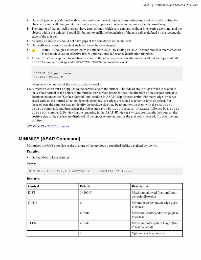
ASAP | Commands and Macros (M) | 225
4. Unit-cell geometry is defined with surface and edge (curve) objects. Lens entities may not be used to define theobjects in a unit cell. Assign interface and scatter properties to objects in the unit cell in the usual way.
5. The interior of the unit cell must not have gaps through which rays can pass without intersecting anything, and theobjects within the unit cell should fill, but not overfill, the boundaries of the unit cell as defined by the rectangularedge of the unit cell.
6. An array of unit cells should not have gaps at the boundaries of the unit cell.7. Unit cells must avoid coincident surfaces when they are arrayed.8. Note: Although a microstructure is defined in ASAP by adding an ASAP scatter model, a microstructure
is not modeled as an effective BRDF (bidirectional reflectance distribution function).9. A microstructure is applied to an object/surface in the same way as any scatter model: call out an object with the
OBJECT command and append a SCATTER MODEL command below it:
OBJECT 'object_name'SCATTER MODEL m
where m is the number of the microstructure model.10. A microstructure must be applied to the correct side of the surface. The side of any ASAP surface is related to
the surface normal at the points of the surface. For surface-based entities, the direction of the surface normal isdocumented under the "Surface Normal" sub-heading in ASAP Help for each entity. For many edge- or curve-based entities, the normal direction depends upon how the edges are joined together to form an object. Forthese objects the simplest way to identify the positive side may be to put rays on them with the EMITTINGOBJECT command, and then render the object and rays with PLOT FACETS OVERLAY followed by a SPOTSPOSITION command. By viewing the rendering in the ASAP 3D viewer ($VIEW command), the spots on thepositive side of the surface are displayed. If the opposite orientation for the unit cell is desired, flip over the unitcell itself.
MICROSTRUCTURE Examples
MINIMIZE (ASAP Command)Minimizes the RMS spot size or the average of the previously specified fields, weighted by the w's.
Function
• Define/Modify Lens Entities
Syntax
MINIMIZE [ w w'...] [ control c ] [ control c' ] ...
Remarks
Control Default Description
DIST 1 (100%) Maximum allowed fractional spot-centroid distortion
GLTH 0 Minimum center and/or edge glassthickness
infinite Maximum center and/or edge glassthickness
TLEN infinite Maximum total system length (firstto last conicoid)
1 Optional starting conicoid
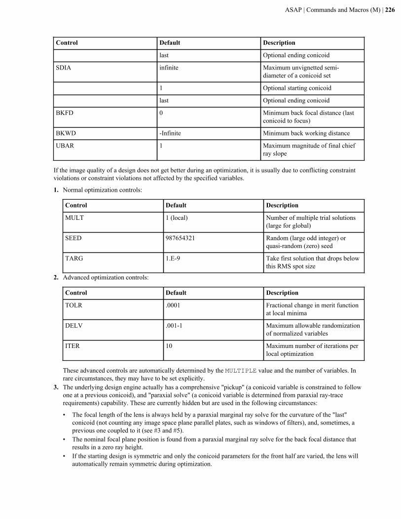
ASAP | Commands and Macros (M) | 226
Control Default Description
last Optional ending conicoid
SDIA infinite Maximum unvignetted semi-diameter of a conicoid set
1 Optional starting conicoid
last Optional ending conicoid
BKFD 0 Minimum back focal distance (lastconicoid to focus)
BKWD -Infinite Minimum back working distance
UBAR 1 Maximum magnitude of final chiefray slope
If the image quality of a design does not get better during an optimization, it is usually due to conflicting constraintviolations or constraint violations not affected by the specified variables.
1. Normal optimization controls:
Control Default Description
MULT 1 (local) Number of multiple trial solutions(large for global)
SEED 987654321 Random (large odd integer) orquasi-random (zero) seed
TARG 1.E-9 Take first solution that drops belowthis RMS spot size
2. Advanced optimization controls:
Control Default Description
TOLR .0001 Fractional change in merit functionat local minima
DELV .001-1 Maximum allowable randomizationof normalized variables
ITER 10 Maximum number of iterations perlocal optimization
These advanced controls are automatically determined by the MULTIPLE value and the number of variables. Inrare circumstances, they may have to be set explicitly.
3. The underlying design engine actually has a comprehensive "pickup" (a conicoid variable is constrained to followone at a previous conicoid), and "paraxial solve" (a conicoid variable is determined from paraxial ray-tracerequirements) capability. These are currently hidden but are used in the following circumstances:
• The focal length of the lens is always held by a paraxial marginal ray solve for the curvature of the "last"conicoid (not counting any image space plane parallel plates, such as windows of filters), and, sometimes, aprevious one coupled to it (see #3 and #5).
• The nominal focal plane position is found from a paraxial marginal ray solve for the back focal distance thatresults in a zero ray height.
• If the starting design is symmetric and only the conicoid parameters for the front half are varied, the lens willautomatically remain symmetric during optimization.
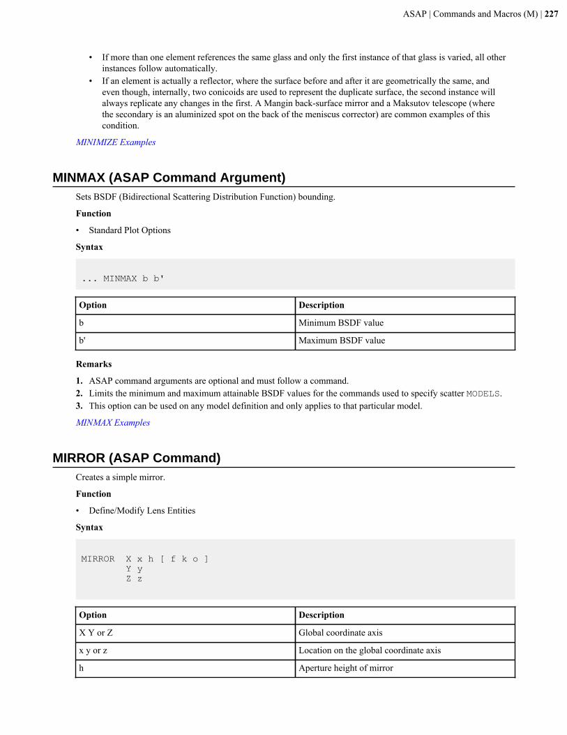
ASAP | Commands and Macros (M) | 227
• If more than one element references the same glass and only the first instance of that glass is varied, all otherinstances follow automatically.
• If an element is actually a reflector, where the surface before and after it are geometrically the same, andeven though, internally, two conicoids are used to represent the duplicate surface, the second instance willalways replicate any changes in the first. A Mangin back-surface mirror and a Maksutov telescope (wherethe secondary is an aluminized spot on the back of the meniscus corrector) are common examples of thiscondition.
MINIMIZE Examples
MINMAX (ASAP Command Argument)Sets BSDF (Bidirectional Scattering Distribution Function) bounding.
Function
• Standard Plot Options
Syntax
... MINMAX b b'
Option Description
b Minimum BSDF value
b' Maximum BSDF value
Remarks
1. ASAP command arguments are optional and must follow a command.2. Limits the minimum and maximum attainable BSDF values for the commands used to specify scatter MODELS.3. This option can be used on any model definition and only applies to that particular model.
MINMAX Examples
MIRROR (ASAP Command)Creates a simple mirror.
Function
• Define/Modify Lens Entities
Syntax
MIRROR X x h [ f k o ] Y y Z z
Option Description
X Y or Z Global coordinate axis
x y or z Location on the global coordinate axis
h Aperture height of mirror
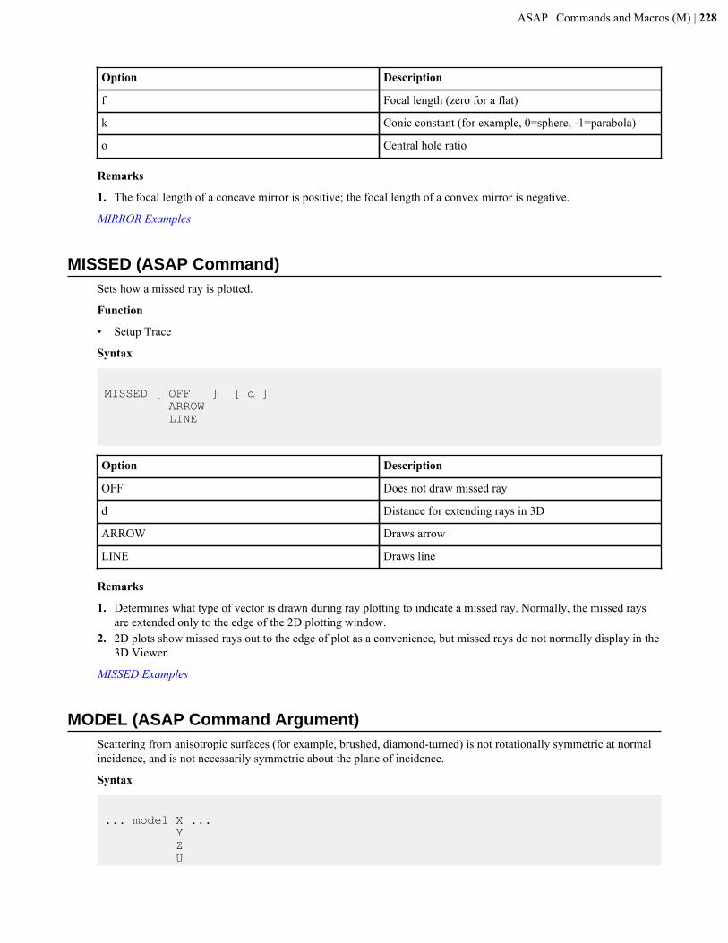
ASAP | Commands and Macros (M) | 228
Option Description
f Focal length (zero for a flat)
k Conic constant (for example, 0=sphere, -1=parabola)
o Central hole ratio
Remarks
1. The focal length of a concave mirror is positive; the focal length of a convex mirror is negative.
MIRROR Examples
MISSED (ASAP Command)Sets how a missed ray is plotted.
Function
• Setup Trace
Syntax
MISSED [ OFF ] [ d ] ARROW LINE
Option Description
OFF Does not draw missed ray
d Distance for extending rays in 3D
ARROW Draws arrow
LINE Draws line
Remarks
1. Determines what type of vector is drawn during ray plotting to indicate a missed ray. Normally, the missed raysare extended only to the edge of the 2D plotting window.
2. 2D plots show missed rays out to the edge of plot as a convenience, but missed rays do not normally display in the3D Viewer.
MISSED Examples
MODEL (ASAP Command Argument)Scattering from anisotropic surfaces (for example, brushed, diamond-turned) is not rotationally symmetric at normalincidence, and is not necessarily symmetric about the plane of incidence.
Syntax
... model X ... Y Z U
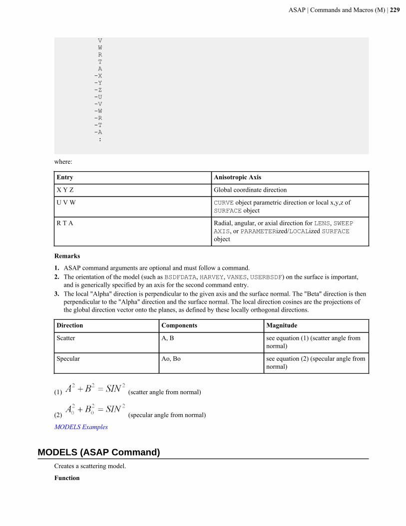
ASAP | Commands and Macros (M) | 229
V W R T A -X -Y -Z -U -V -W -R -T -A :
where:
Entry Anisotropic Axis
X Y Z Global coordinate direction
U V W CURVE object parametric direction or local x,y,z ofSURFACE object
R T A Radial, angular, or axial direction for LENS, SWEEPAXIS, or PARAMETERized/LOCALized SURFACEobject
Remarks
1. ASAP command arguments are optional and must follow a command.2. The orientation of the model (such as BSDFDATA, HARVEY, VANES, USERBSDF) on the surface is important,
and is generically specified by an axis for the second command entry.3. The local "Alpha" direction is perpendicular to the given axis and the surface normal. The "Beta" direction is then
perpendicular to the "Alpha" direction and the surface normal. The local direction cosines are the projections ofthe global direction vector onto the planes, as defined by these locally orthogonal directions.
Direction Components Magnitude
Scatter A, B see equation (1) (scatter angle fromnormal)
Specular Ao, Bo see equation (2) (specular angle fromnormal)
(1) (scatter angle from normal)
(2) (specular angle from normal)
MODELS Examples
MODELS (ASAP Command)Creates a scattering model.
Function
ASAP | Commands and Macros (M) | 230
• Create/Modify Media, Coatings, Scatter Models
Syntax
MODELS [ i [ PLOT [ a a'...] ] ]
Option Description
i Beginning model number
PLOT Plots the model in log (b-bo) and angle space
a a' ... User-defined degree specular angles
Remarks
1. Defines a specific scatter model from a general set of Bi-directional Scattering Distribution Function (BSDF)scattering models.
2. Begin defining scatter MODELS at number i (the default model number is one more than the highest defined).3. Similar to the MEDIA and the COATING commands, it constructs a database for use in the construction of an
OBJECT.4. Creates a distribution file name_angle.dis for each of these angles.5. Both the r and t values on the INTERFACE command must be non-zero.6. The command argument, MINMAX may be used to set the minimum and maximum values of the BSDF for this
specific model.
MODELS Examples
MODIFY (ASAP Command)Modifies current distribution data.
Function
• Display/Modify Data Distributions
Syntax
MODIFY [ m m' n n' [ a b ] ] [ 'flabel' ] fcn[ m m' n n' [ a b ] ] fcn :
Option Description
m m' Integer pixel ranges in the across direction
n n' Integer pixel ranges in the down direction
a b Scale factors
fcn Internally or user-defined function
'flabel' Optional text to relabel the functional data
Remarks
1. Modifies the data region specified by the two integer pixel ranges, m to m' (across) and n to n' (down). The data inthat region is replaced by a plus b times the data value, that is:
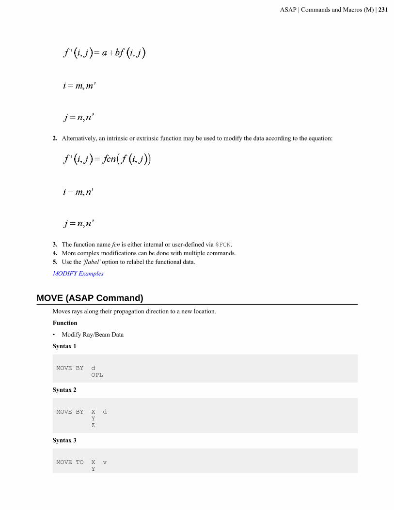
ASAP | Commands and Macros (M) | 231
2. Alternatively, an intrinsic or extrinsic function may be used to modify the data according to the equation:
3. The function name fcn is either internal or user-defined via $FCN.4. More complex modifications can be done with multiple commands.5. Use the 'flabel' option to relabel the functional data.
MODIFY Examples
MOVE (ASAP Command)Moves rays along their propagation direction to a new location.
Function
• Modify Ray/Beam Data
Syntax 1
MOVE BY d OPL
Syntax 2
MOVE BY X d Y Z
Syntax 3
MOVE TO X v Y

ASAP | Commands and Macros (M) | 232
Z
Option Description
BY Relative move
TO Absolute move
d Distance along a given coordinate direction
X Y Z Direction vectors
OPL Optical path length
v Value for location of ray intersection
Remarks for Syntax 1
1. MOVEs rays along their direction vectors BY the specified distance d, or projected distance along direction vectorX, Y, or Z.
2. MOVEs rays along their direction vectors BY the specified OPL, accounting for the index of the media in which therays currently exist.
Remarks for Syntax 2
1. MOVEs the rays along their direction vectors BY the projected distance d along the specified axis.
Remarks for Syntax 3
1. MOVEs rays along their direction vectors TO the specified location value v or to the point of closest approach if theprojection vector does not intersect value v.
Remarks - General
1. During the MOVE operation, the rays are projected along their direction vectors. The rays do not intersect anyOBJECTS along the way.
2. Commonly used for virtual ray tracing from a buried entrance pupil to object space, so that the beam may then betraced through the system.
3. Use MOVE to observe the effects of defocus on a beam.
MOVE Examples
MOVE PARABASALS (ASAP Command)Moves the parabasal rays for each ray/beam to its base ray plane.
Function
• Modify Ray/Beam Data
Syntax
MOVE PARABASALS
Remarks
1. Moves parabasals to a plane perpendicular to the base point. It does not in any way change the beamcharacteristics, but does affect the PLOT BEAMS display since, by default, the parabasals lie on the current objectsurface.
MOVE Examples
ASAP | Commands and Macros (M) | 233
MOVE TO FOCI (ASAP Command)Moves rays or beams along the propagation direction to a focus determined by the plane of minimum RMS spot size.
Function
• Modify Ray/Beam Data
Syntax
MOVE TO FOCI [ n n' n" ... ]
Option Description
n n' n" ... Specified parabasal rays
Remarks
1. Moves each ray/beam to the centroid of the intersections of the given parabasal rays with the base ray.
MOVE Examples
MOVE TO PLANE (ASAP Command)Moves rays along their propagation direction to a specified reference plane.
Function
• Modify Ray/Beam Data
Syntax
MOVE TO PLANE [ x y z ] [ a,b,c ]
Option Description
x y z Global coordinate of a reference plane
a,b,c Global direction vector of the surface normal of theplane
Remarks
1. Transfers the current ray/beam set to a plane with normal (a,b,c) through the point (x,y,z).2. The default point is the average of the current base ray coordinates.3. The default for the normal to the plane is the average of the current base ray directions.4. The peak-to-valley optical path difference on this surface is also printed so that normally it represents the
reference plane of an afocal system.
MOVE TO PLANE Examples
MOVE TO POINT (ASAP Command)Moves rays along their trajectories to their closest approach to the given point (x y z).
Function
• Modify Ray/Beam Data
ASAP | Commands and Macros (M) | 234
Syntax
MOVE TO POINT x y z
MOVE TO POINT Examples
MOVE TO SPHERE (ASAP Command)Moves rays along their propagation direction to a specified different sphere.
Function
• Modify Ray/Beam Data
Syntax
MOVE TO SPHERE r [ x y z ]
Option Description
r Radius of reference sphere
x y z Coordinate of center of reference sphere
Remarks
1. Transfers the current ray/beam set to the surface of a sphere of radius r centered on the point (x,y,z) or a PLANEwith normal (a,b,c) through point (x, y, z) by using the variation of the MOVE command.
2. The default point is the average of the current base ray coordinates.3. The peak-to-valley optical path difference on this surface is also printed so that normally it represents the
reference sphere of a focusing system.4. If none of the SPHERE data is given, a best-fit spherical wavefront is used.5. The default for the normal to the PLANE is the average of the current base ray directions.6. The default point is the average of the current base ray coordinates.7. The peak-to-valley and RMS optical path difference on this surface are also printed so that normally it represents
either the reference sphere of a focussing system or the reference plane of an afocal system.
MOVE TO SPHERE Examples
$MSGS (ASAP Macro)Switch on or off the display of warning and informative messages other than error messages.
Syntax
$MSGS [ ON ] OFF
$MSGS Examples
MUELLER (ASAP Command)Creates Mueller matrix elements.
Function
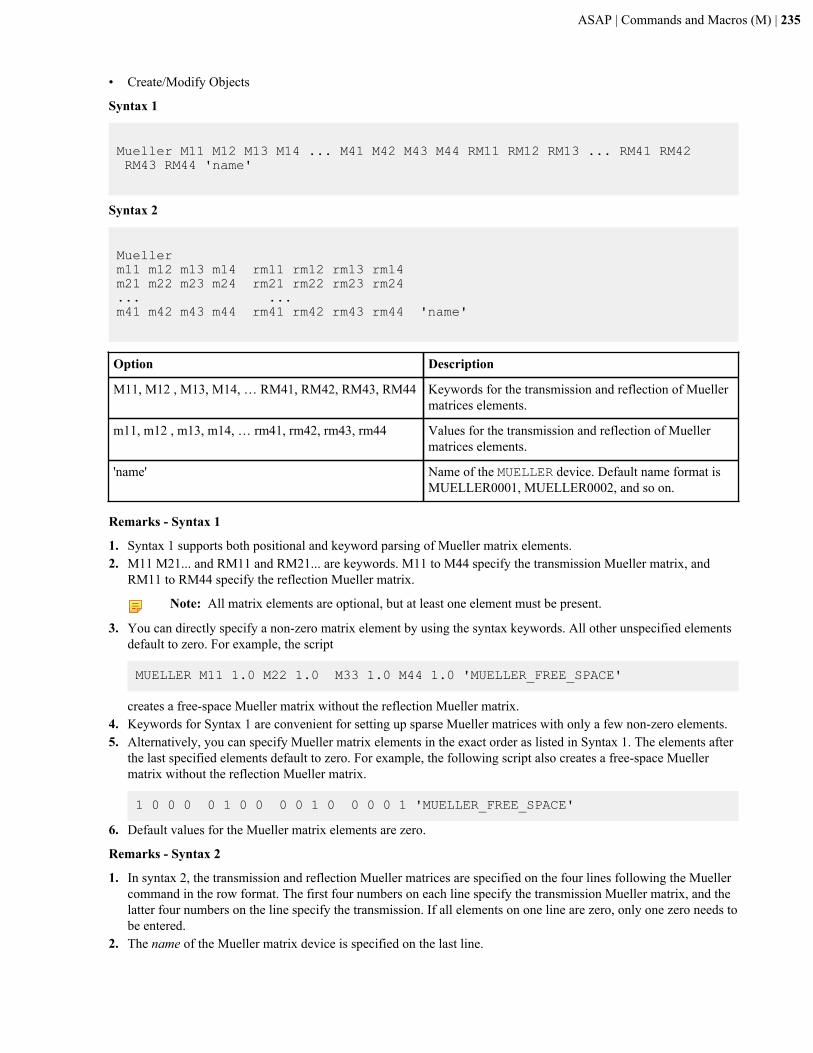
ASAP | Commands and Macros (M) | 235
• Create/Modify Objects
Syntax 1
Mueller M11 M12 M13 M14 ... M41 M42 M43 M44 RM11 RM12 RM13 ... RM41 RM42 RM43 RM44 'name'
Syntax 2
Mueller m11 m12 m13 m14 rm11 rm12 rm13 rm14m21 m22 m23 m24 rm21 rm22 rm23 rm24... ... m41 m42 m43 m44 rm41 rm42 rm43 rm44 'name'
Option Description
M11, M12 , M13, M14, … RM41, RM42, RM43, RM44 Keywords for the transmission and reflection of Muellermatrices elements.
m11, m12 , m13, m14, … rm41, rm42, rm43, rm44 Values for the transmission and reflection of Muellermatrices elements.
'name' Name of the MUELLER device. Default name format isMUELLER0001, MUELLER0002, and so on.
Remarks - Syntax 1
1. Syntax 1 supports both positional and keyword parsing of Mueller matrix elements.2. M11 M21... and RM11 and RM21... are keywords. M11 to M44 specify the transmission Mueller matrix, and
RM11 to RM44 specify the reflection Mueller matrix.
Note: All matrix elements are optional, but at least one element must be present.
3. You can directly specify a non-zero matrix element by using the syntax keywords. All other unspecified elementsdefault to zero. For example, the script
MUELLER M11 1.0 M22 1.0 M33 1.0 M44 1.0 'MUELLER_FREE_SPACE'
creates a free-space Mueller matrix without the reflection Mueller matrix.4. Keywords for Syntax 1 are convenient for setting up sparse Mueller matrices with only a few non-zero elements.5. Alternatively, you can specify Mueller matrix elements in the exact order as listed in Syntax 1. The elements after
the last specified elements default to zero. For example, the following script also creates a free-space Muellermatrix without the reflection Mueller matrix.
1 0 0 0 0 1 0 0 0 0 1 0 0 0 0 1 'MUELLER_FREE_SPACE'
6. Default values for the Mueller matrix elements are zero.
Remarks - Syntax 2
1. In syntax 2, the transmission and reflection Mueller matrices are specified on the four lines following the Muellercommand in the row format. The first four numbers on each line specify the transmission Mueller matrix, and thelatter four numbers on the line specify the transmission. If all elements on one line are zero, only one zero needs tobe entered.
2. The name of the Mueller matrix device is specified on the last line.
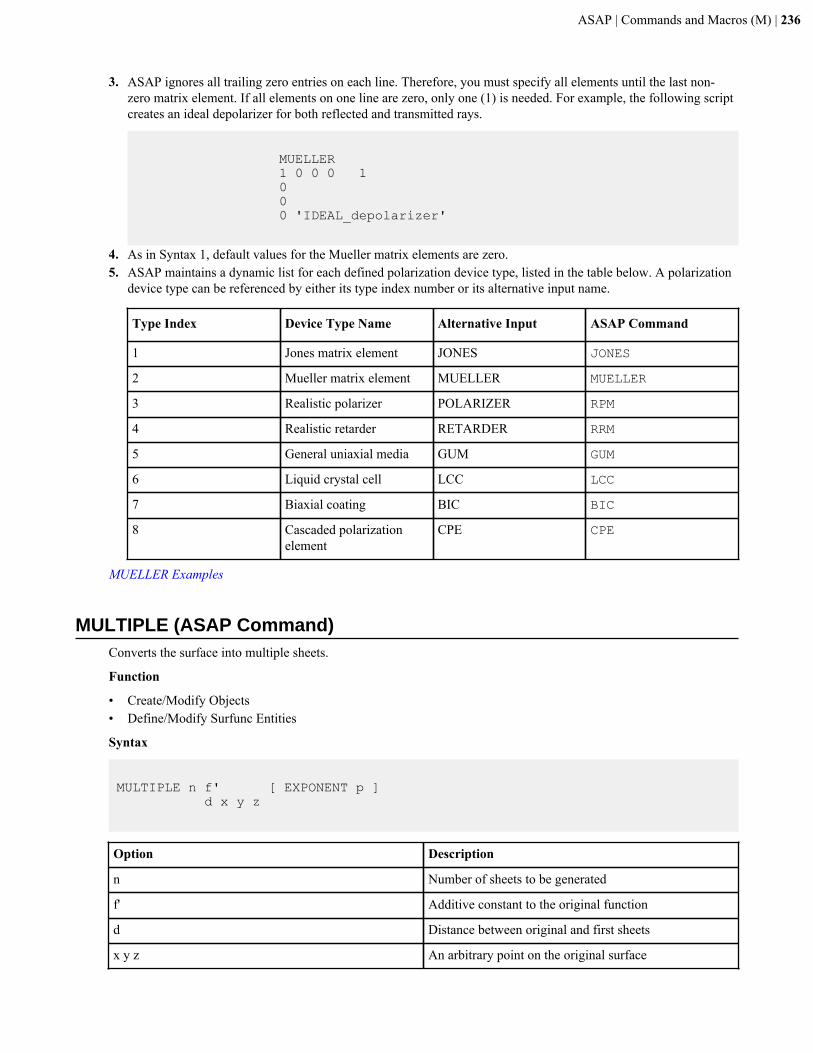
ASAP | Commands and Macros (M) | 236
3. ASAP ignores all trailing zero entries on each line. Therefore, you must specify all elements until the last non-zero matrix element. If all elements on one line are zero, only one (1) is needed. For example, the following scriptcreates an ideal depolarizer for both reflected and transmitted rays.
MUELLER 1 0 0 0 1 0 0 0 'IDEAL_depolarizer'
4. As in Syntax 1, default values for the Mueller matrix elements are zero.5. ASAP maintains a dynamic list for each defined polarization device type, listed in the table below. A polarization
device type can be referenced by either its type index number or its alternative input name.
Type Index Device Type Name Alternative Input ASAP Command
1 Jones matrix element JONES JONES
2 Mueller matrix element MUELLER MUELLER
3 Realistic polarizer POLARIZER RPM
4 Realistic retarder RETARDER RRM
5 General uniaxial media GUM GUM
6 Liquid crystal cell LCC LCC
7 Biaxial coating BIC BIC
8 Cascaded polarizationelement
CPE CPE
MUELLER Examples
MULTIPLE (ASAP Command)Converts the surface into multiple sheets.
Function
• Create/Modify Objects• Define/Modify Surfunc Entities
Syntax
MULTIPLE n f' [ EXPONENT p ] d x y z
Option Description
n Number of sheets to be generated
f' Additive constant to the original function
d Distance between original and first sheets
x y z An arbitrary point on the original surface
ASAP | Commands and Macros (M) | 237
Option Description
EXPONENT p Exponent to which sheet number is raised
Remarks
1. The surface is converted into multiple parallel surfaces. In other words, the equation of the surfaces becomes:
2. The zeroth sheet is the original surface.3. Alternatively, ASAP can calculate f' such that the distance from a point x,y,z on the original surface to the first
sheet is d.4. The exponent p is defaulted to 1, but can be used, for example, to get evenly spaced cylinders or spheres (p=2).5. If MULTIPLE is being used to define a diffraction grating, then the value of n is irrelevant.6. Graphical viewing (for example, PROFILES or RENDER) of changes to sheet spacing that use the EXPONENT
option is not possible. Instead, verification may be made after tracing an INTERFACE...DIFFRACT object thatreferences this multiple surface.
MULTIPLE Examples
ASAP | Commands and Macros (N-O) | 238
Commands and Macros (N-O)
Topics in this section of the Contents tab include ASAP commands and macros that begin with the letter “N-O”.
$NEXT (ASAP Macro)Immediately begins processing of the next $DO or $ITER iteration by forcing a branch to the top of the current loopblock.
Syntax
$NEXT
Example
$DO 1 10{ :
This block is executed every iteration:$IF ? LE 5; $NEXT:This block is executed only for iterations 6 through 10:
$NEXT Examples
NONLINEAR (ASAP Command)Creates a scatter model based on the combination of the Phong and Harvey models.
Function
• Create/Modify Media, Coatings, Scatter Models
Syntax 1- Isotropic (polynomial coefficients)
NONLINEAR a1 b1 c1 d1 e1 [ a2' b2' c2' d2' e2' [ a3" b3" c3" d3" e3" ...] ] ] [ PLOT [ a a' ...] ]
Syntax 2 - Anisotropic
NONLINEAR X p q a b c d e [ p' q' a' b' c' d' e' ... ] ] Y Z :
Syntax 3 - Fitting BSDF values
NONLINEAR FIT [ n ] [ options ] FRAC e e' ...
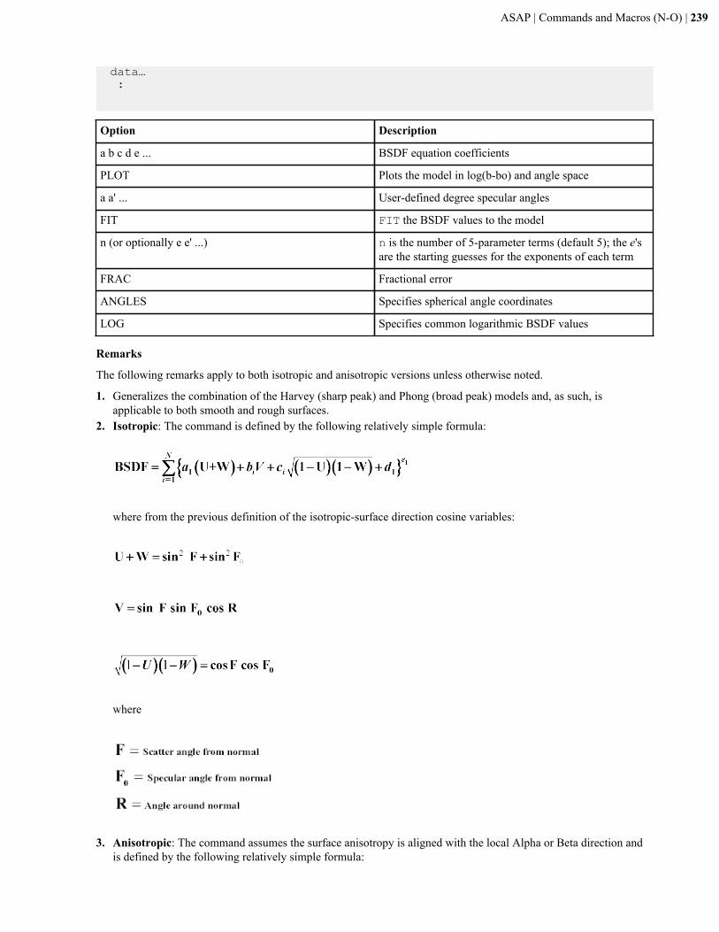
ASAP | Commands and Macros (N-O) | 239
data… :
Option Description
a b c d e ... BSDF equation coefficients
PLOT Plots the model in log(b-bo) and angle space
a a' ... User-defined degree specular angles
FIT FIT the BSDF values to the model
n (or optionally e e' ...) n is the number of 5-parameter terms (default 5); the e'sare the starting guesses for the exponents of each term
FRAC Fractional error
ANGLES Specifies spherical angle coordinates
LOG Specifies common logarithmic BSDF values
Remarks
The following remarks apply to both isotropic and anisotropic versions unless otherwise noted.
1. Generalizes the combination of the Harvey (sharp peak) and Phong (broad peak) models and, as such, isapplicable to both smooth and rough surfaces.
2. Isotropic: The command is defined by the following relatively simple formula:
where from the previous definition of the isotropic-surface direction cosine variables:
where
3. Anisotropic: The command assumes the surface anisotropy is aligned with the local Alpha or Beta direction and
is defined by the following relatively simple formula:
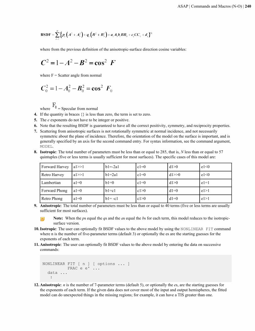
ASAP | Commands and Macros (N-O) | 240
where from the previous definition of the anisotropic-surface direction cosine variables:
where F = Scatter angle from normal
where = Specular from normal4. If the quantity in braces {} is less than zero, the term is set to zero.5. The e exponents do not have to be integer or positive.6. Note that the resulting BSDF is guaranteed to have all the correct positivity, symmetry, and reciprocity properties.7. Scattering from anisotropic surfaces is not rotationally symmetric at normal incidence, and not necessarily
symmetric about the plane of incidence. Therefore, the orientation of the model on the surface is important, and isgenerally specified by an axis for the second command entry. For syntax information, see the command argument,MODEL.
8. Isotropic: The total number of parameters must be less than or equal to 285, that is, N less than or equal to 57quintuples (five or less terms is usually sufficient for most surfaces). The specific cases of this model are:
Forward Harvey a1>>1 b1=-2a1 c1=0 d1>0 e1<0
Retro Harvey a1>>1 b1=2a1 c1=0 d1>>0 e1<0
Lambertian a1=0 b1=0 c1=0 d1>0 e1=1
Forward Phong a1=0 b1=c1 c1>0 d1=0 e1>1
Retro Phong a1=0 b1= -c1 c1>0 d1=0 e1>1
9. Anisotropic: The total number of parameters must be less than or equal to 40 terms (five or less terms are usuallysufficient for most surfaces).
Note: When the ps equal the qs and the as equal the bs for each term, this model reduces to the isotropic-surface version.
10. Isotropic: The user can optionally fit BSDF values to the above model by using the NONLINEAR FIT commandwhere n is the number of five-parameter terms (default 3) or optionally the es are the starting guesses for theexponents of each term.
11. Anisotropic: The user can optionally fit BSDF values to the above model by entering the data on successivecommands:
NONLINEAR FIT [ n ] [ options ... ] FRAC e e' ... data ... :
12. Anisotropic: n is the number of 7-parameter terms (default 5), or optionally the es, are the starting guesses forthe exponents of each term. If the given data does not cover most of the input and output hemispheres, the fittedmodel can do unexpected things in the missing regions; for example, it can have a TIS greater than one.
ASAP | Commands and Macros (N-O) | 241
13. Since the NONLINEAR model is not defined in logarithm space (like the POLYNOMIAL model), the FIT mayhave difficulty in accurately reproducing any BSDF with a high dynamic range. Optionally, the FRACtional errorat each data point can be used instead of the absolute error. This has about the same effect as fitting in logarithmspace. In either case, the fit is done using an iterative non-linear damped least-squares algorithm. Therefore,it converges to one of the local minima and not necessarily the best one. An off-line, time-consuming, globaloptimization technique (for example, simulated annealing) could be used if the data only needs to be fit once.
14. The PLOT option plots the model (common base 10 logarithm of the BSDF) for up to seven specular angles inascending order (default 0, 15, 30, 45, 60, 75, 89.9 degrees). The current PIXELS setting controls the resolutionof these plots in direction cosine space, and it creates a distribution file, name_angle.dis for each of these angles.
15. The command argument, MINMAX may be used to set the minimum and maximum values of the BSDF for thisspecific model.
NONLINEAR Examples
NORMALIZE (ASAP Command)Renormalizes the current distribution data.
Function
• Display/Modify Data Distributions
Syntax
NORMALIZE [ d [ v [ h ] ] ] [ 'flabel' ] MAX MAX
Option Description
d Data renormalization value
v Vertical scale factor
h Horizontal scale factor
MAX Maximum distribution data or coordinate value
'flabel' New label for functional data
Remarks
1. Renormalizes distribution data (divides functional values) by the value of the last NORMALIZE command(default).
2. Alternatively, the data may be normalized by the given value d or the MAXimum value in the distribution data.3. Vertical v and horizontal h coordinate ranges can also be normalized in a similar manner by the optional third and
fourth entries.4. Use the flabel option to relabel the functional data.5. Different scale factors can be used for the two coordinate ranges.
NORMALIZE Examples
NUMBERS (ASAP Command)Displays current valid media, surfaces, edges, lenses, and object numbers.
Function
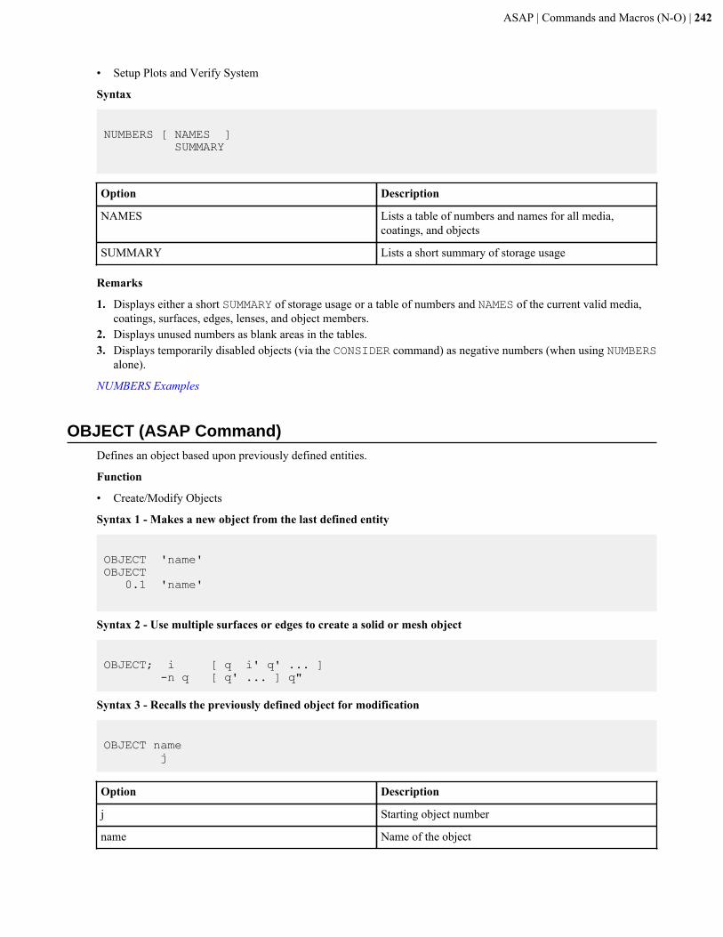
ASAP | Commands and Macros (N-O) | 242
• Setup Plots and Verify System
Syntax
NUMBERS [ NAMES ] SUMMARY
Option Description
NAMES Lists a table of numbers and names for all media,coatings, and objects
SUMMARY Lists a short summary of storage usage
Remarks
1. Displays either a short SUMMARY of storage usage or a table of numbers and NAMES of the current valid media,coatings, surfaces, edges, lenses, and object members.
2. Displays unused numbers as blank areas in the tables.3. Displays temporarily disabled objects (via the CONSIDER command) as negative numbers (when using NUMBERS
alone).
NUMBERS Examples
OBJECT (ASAP Command)Defines an object based upon previously defined entities.
Function
• Create/Modify Objects
Syntax 1 - Makes a new object from the last defined entity
OBJECT 'name' OBJECT 0.1 'name'
Syntax 2 - Use multiple surfaces or edges to create a solid or mesh object
OBJECT; i [ q i' q' ... ] -n q [ q' ... ] q"
Syntax 3 - Recalls the previously defined object for modification
OBJECT name j
Option Description
j Starting object number
name Name of the object
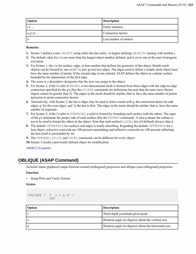
ASAP | Commands and Macros (N-O) | 243
Option Description
i i' ... Entity numbers
q q' q" ... Connection factors
n Last number of entities
Remarks
1. Syntax 1 defines a new OBJECT using either the last entity, or begins defining OBJECTS starting with number j.2. The default value for j is one more than the largest object number defined, and is set to one at the start of program
execution.3. For Syntax 1, the i is the surface, edge, or lens number that defines the geometry of the object. Simple mesh
objects can be formed by one or (if i' is also given) two edges. The edges used to define a simple mesh object musthave the same number of points. If the second edge is not entered, ASAP defines the object as a planar surfacebounded by the dimensions of the first edge.
4. The name is a descriptive designator that the user can assign to the object.5. For Syntax 2, if the i's refer to EDGES, a two-dimensional mesh is formed from these edges with the edge-to-edge
connection specified by the q's (See the POINTS commands for definitions but note that the inter-curve Bezierdegree cannot be greater than 2). The edges in the mesh should be similar; that is, have the same number of pointsand point-to-point connection factors.
6. Alternatively, with Syntax 2, the last n edges may be used to form a mesh with q, the connection factor for oddedges, q' for the even edges, and "q the last to first. The edges in the mesh should be similar; that is, have the samenumber of segments.
7. For Syntax 2, if the i's refer to SURFACES, a solid is formed by bounding each surface with the others. The signsof the q's determine the proper side of each surface (See the BOUNDS command). A zero q means the surface isnot to be used to bound the others in the object. Note that each surface's LOCAL box (if defined) always clips it.
8. The default INTERFACE for surfaces and edges is totally absorbing. Regarding the default INTERFACE for alens object, refractive conicoids are 100 percent transmitting and reflective conicoids are 100 percent reflecting;the lens itself is surrounded by air.
9. The FRESNEL, SPLIT, and LEVEL commands can be different for every object.10. Syntax 3 recalls a previously defined object for modification.
OBJECT Examples
OBLIQUE (ASAP Command)Switches future graphical output between normal (orthogonal) projection and oblique (non-orthogonal) projection.
Function
• Setup Plots and Verify System
Syntax
OBLIQUE [ f ] [ a a' ] OFF
Option Description
f Third depth coordinate pivot point
a Rotation angle (in degrees) about the vertical axis
a' Rotation angle (in degrees) about the horizontal axis
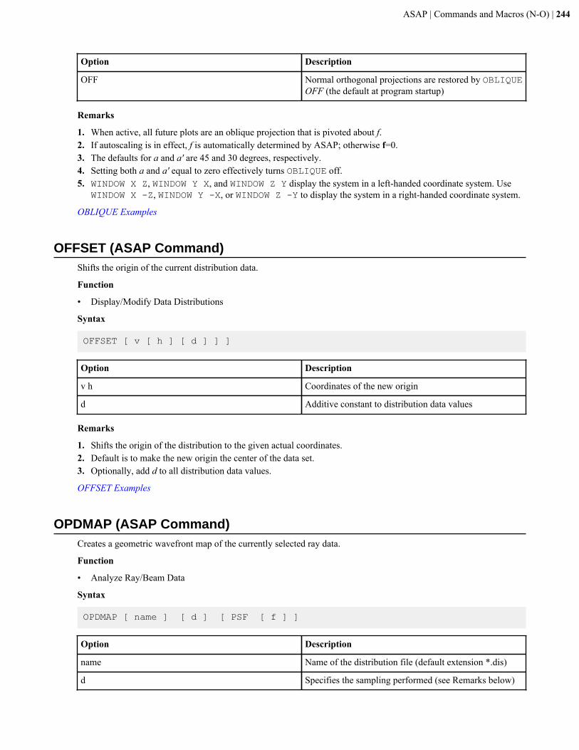
ASAP | Commands and Macros (N-O) | 244
Option Description
OFF Normal orthogonal projections are restored by OBLIQUEOFF (the default at program startup)
Remarks
1. When active, all future plots are an oblique projection that is pivoted about f.2. If autoscaling is in effect, f is automatically determined by ASAP; otherwise f=0.3. The defaults for a and a' are 45 and 30 degrees, respectively.4. Setting both a and a' equal to zero effectively turns OBLIQUE off.5. WINDOW X Z, WINDOW Y X, and WINDOW Z Y display the system in a left-handed coordinate system. Use
WINDOW X -Z, WINDOW Y -X, or WINDOW Z -Y to display the system in a right-handed coordinate system.
OBLIQUE Examples
OFFSET (ASAP Command)Shifts the origin of the current distribution data.
Function
• Display/Modify Data Distributions
Syntax
OFFSET [ v [ h ] [ d ] ] ]
Option Description
v h Coordinates of the new origin
d Additive constant to distribution data values
Remarks
1. Shifts the origin of the distribution to the given actual coordinates.2. Default is to make the new origin the center of the data set.3. Optionally, add d to all distribution data values.
OFFSET Examples
OPDMAP (ASAP Command)Creates a geometric wavefront map of the currently selected ray data.
Function
• Analyze Ray/Beam Data
Syntax
OPDMAP [ name ] [ d ] [ PSF [ f ] ]
Option Description
name Name of the distribution file (default extension *.dis)
d Specifies the sampling performed (see Remarks below)
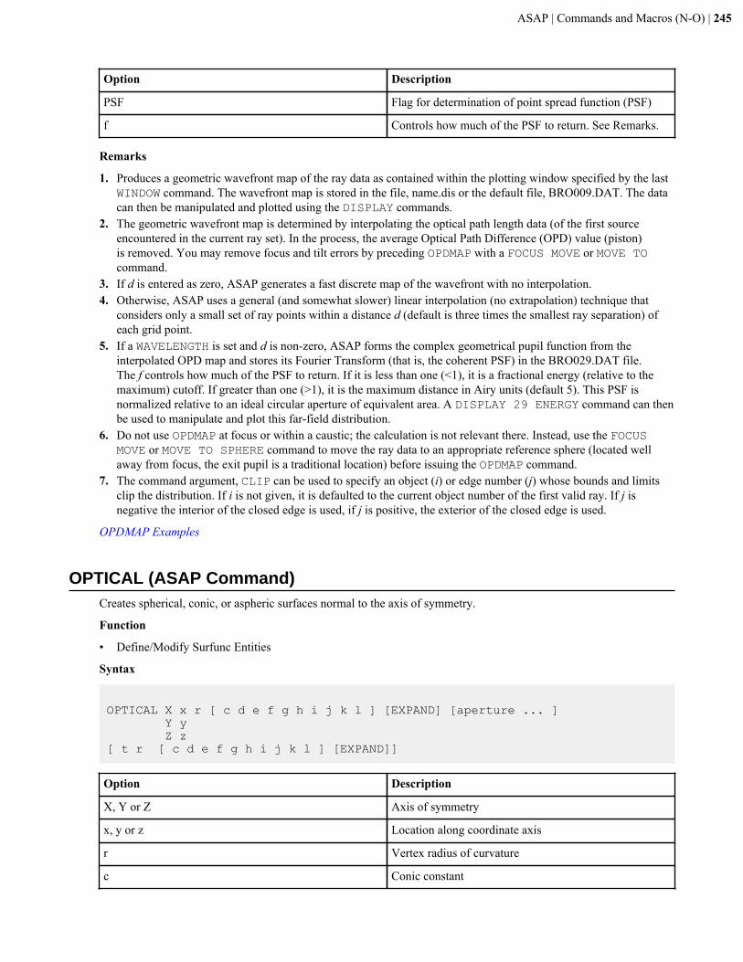
ASAP | Commands and Macros (N-O) | 245
Option Description
PSF Flag for determination of point spread function (PSF)
f Controls how much of the PSF to return. See Remarks.
Remarks
1. Produces a geometric wavefront map of the ray data as contained within the plotting window specified by the lastWINDOW command. The wavefront map is stored in the file, name.dis or the default file, BRO009.DAT. The datacan then be manipulated and plotted using the DISPLAY commands.
2. The geometric wavefront map is determined by interpolating the optical path length data (of the first sourceencountered in the current ray set). In the process, the average Optical Path Difference (OPD) value (piston)is removed. You may remove focus and tilt errors by preceding OPDMAP with a FOCUS MOVE or MOVE TOcommand.
3. If d is entered as zero, ASAP generates a fast discrete map of the wavefront with no interpolation.4. Otherwise, ASAP uses a general (and somewhat slower) linear interpolation (no extrapolation) technique that
considers only a small set of ray points within a distance d (default is three times the smallest ray separation) ofeach grid point.
5. If a WAVELENGTH is set and d is non-zero, ASAP forms the complex geometrical pupil function from theinterpolated OPD map and stores its Fourier Transform (that is, the coherent PSF) in the BRO029.DAT file.The f controls how much of the PSF to return. If it is less than one (<1), it is a fractional energy (relative to themaximum) cutoff. If greater than one (>1), it is the maximum distance in Airy units (default 5). This PSF isnormalized relative to an ideal circular aperture of equivalent area. A DISPLAY 29 ENERGY command can thenbe used to manipulate and plot this far-field distribution.
6. Do not use OPDMAP at focus or within a caustic; the calculation is not relevant there. Instead, use the FOCUSMOVE or MOVE TO SPHERE command to move the ray data to an appropriate reference sphere (located wellaway from focus, the exit pupil is a traditional location) before issuing the OPDMAP command.
7. The command argument, CLIP can be used to specify an object (i) or edge number (j) whose bounds and limitsclip the distribution. If i is not given, it is defaulted to the current object number of the first valid ray. If j isnegative the interior of the closed edge is used, if j is positive, the exterior of the closed edge is used.
OPDMAP Examples
OPTICAL (ASAP Command)Creates spherical, conic, or aspheric surfaces normal to the axis of symmetry.
Function
• Define/Modify Surfunc Entities
Syntax
OPTICAL X x r [ c d e f g h i j k l ] [EXPAND] [aperture ... ] Y y Z z[ t r [ c d e f g h i j k l ] [EXPAND]]
Option Description
X, Y or Z Axis of symmetry
x, y or z Location along coordinate axis
r Vertex radius of curvature
c Conic constant
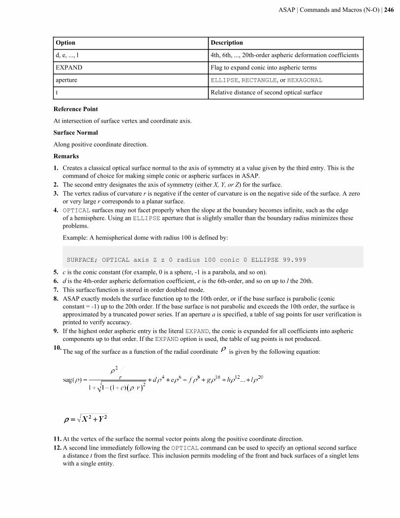
ASAP | Commands and Macros (N-O) | 246
Option Description
d, e, ..., l 4th, 6th, ..., 20th-order aspheric deformation coefficients
EXPAND Flag to expand conic into aspheric terms
aperture ELLIPSE, RECTANGLE, or HEXAGONAL
t Relative distance of second optical surface
Reference Point
At intersection of surface vertex and coordinate axis.
Surface Normal
Along positive coordinate direction.
Remarks
1. Creates a classical optical surface normal to the axis of symmetry at a value given by the third entry. This is thecommand of choice for making simple conic or aspheric surfaces in ASAP.
2. The second entry designates the axis of symmetry (either X, Y, or Z) for the surface.3. The vertex radius of curvature r is negative if the center of curvature is on the negative side of the surface. A zero
or very large r corresponds to a planar surface.4. OPTICAL surfaces may not facet properly when the slope at the boundary becomes infinite, such as the edge
of a hemisphere. Using an ELLIPSE aperture that is slightly smaller than the boundary radius minimizes theseproblems.
Example: A hemispherical dome with radius 100 is defined by:
SURFACE; OPTICAL axis Z z 0 radius 100 conic 0 ELLIPSE 99.999
5. c is the conic constant (for example, 0 is a sphere, -1 is a parabola, and so on).6. d is the 4th-order aspheric deformation coefficient, e is the 6th-order, and so on up to l the 20th.7. This surface/function is stored in order doubled mode.8. ASAP exactly models the surface function up to the 10th order, or if the base surface is parabolic (conic
constant = -1) up to the 20th order. If the base surface is not parabolic and exceeds the 10th order, the surface isapproximated by a truncated power series. If an aperture a is specified, a table of sag points for user verification isprinted to verify accuracy.
9. If the highest order aspheric entry is the literal EXPAND, the conic is expanded for all coefficients into asphericcomponents up to that order. If the EXPAND option is used, the table of sag points is not produced.
10. The sag of the surface as a function of the radial coordinate is given by the following equation:
11. At the vertex of the surface the normal vector points along the positive coordinate direction.12. A second line immediately following the OPTICAL command can be used to specify an optional second surface
a distance t from the first surface. This inclusion permits modeling of the front and back surfaces of a singlet lenswith a single entity.
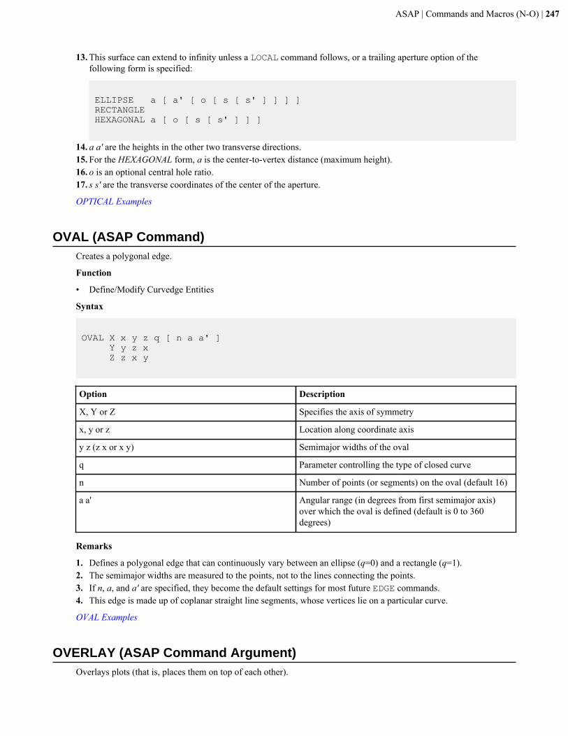
ASAP | Commands and Macros (N-O) | 247
13. This surface can extend to infinity unless a LOCAL command follows, or a trailing aperture option of thefollowing form is specified:
ELLIPSE a [ a' [ o [ s [ s' ] ] ] ]RECTANGLEHEXAGONAL a [ o [ s [ s' ] ] ]
14. a a' are the heights in the other two transverse directions.15. For the HEXAGONAL form, a is the center-to-vertex distance (maximum height).16. o is an optional central hole ratio.17. s s' are the transverse coordinates of the center of the aperture.
OPTICAL Examples
OVAL (ASAP Command)Creates a polygonal edge.
Function
• Define/Modify Curvedge Entities
Syntax
OVAL X x y z q [ n a a' ] Y y z x Z z x y
Option Description
X, Y or Z Specifies the axis of symmetry
x, y or z Location along coordinate axis
y z (z x or x y) Semimajor widths of the oval
q Parameter controlling the type of closed curve
n Number of points (or segments) on the oval (default 16)
a a' Angular range (in degrees from first semimajor axis)over which the oval is defined (default is 0 to 360degrees)
Remarks
1. Defines a polygonal edge that can continuously vary between an ellipse (q=0) and a rectangle (q=1).2. The semimajor widths are measured to the points, not to the lines connecting the points.3. If n, a, and a' are specified, they become the default settings for most future EDGE commands.4. This edge is made up of coplanar straight line segments, whose vertices lie on a particular curve.
OVAL Examples
OVERLAY (ASAP Command Argument)Overlays plots (that is, places them on top of each other).
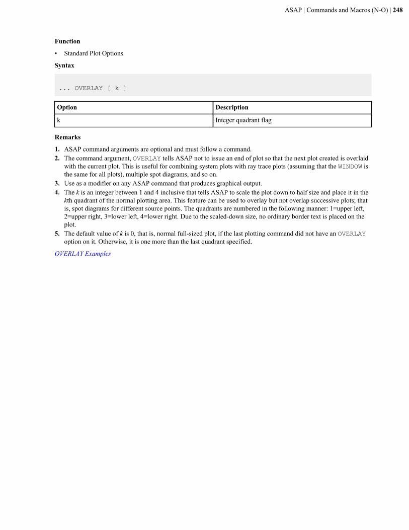
ASAP | Commands and Macros (N-O) | 248
Function
• Standard Plot Options
Syntax
... OVERLAY [ k ]
Option Description
k Integer quadrant flag
Remarks
1. ASAP command arguments are optional and must follow a command.2. The command argument, OVERLAY tells ASAP not to issue an end of plot so that the next plot created is overlaid
with the current plot. This is useful for combining system plots with ray trace plots (assuming that the WINDOW isthe same for all plots), multiple spot diagrams, and so on.
3. Use as a modifier on any ASAP command that produces graphical output.4. The k is an integer between 1 and 4 inclusive that tells ASAP to scale the plot down to half size and place it in the
kth quadrant of the normal plotting area. This feature can be used to overlay but not overlap successive plots; thatis, spot diagrams for different source points. The quadrants are numbered in the following manner: 1=upper left,2=upper right, 3=lower left, 4=lower right. Due to the scaled-down size, no ordinary border text is placed on theplot.
5. The default value of k is 0, that is, normal full-sized plot, if the last plotting command did not have an OVERLAYoption on it. Otherwise, it is one more than the last quadrant specified.
OVERLAY Examples
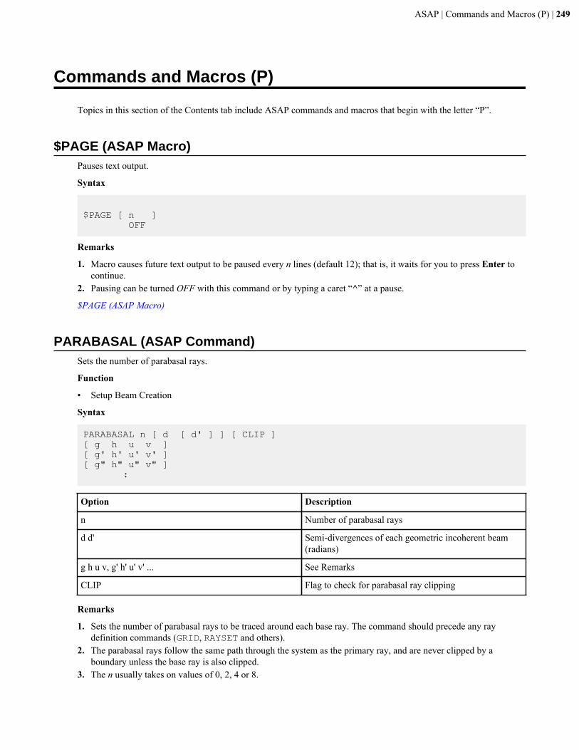
ASAP | Commands and Macros (P) | 249
Commands and Macros (P)
Topics in this section of the Contents tab include ASAP commands and macros that begin with the letter “P”.
$PAGE (ASAP Macro)Pauses text output.
Syntax
$PAGE [ n ] OFF
Remarks
1. Macro causes future text output to be paused every n lines (default 12); that is, it waits for you to press Enter tocontinue.
2. Pausing can be turned OFF with this command or by typing a caret “^” at a pause.
$PAGE (ASAP Macro)
PARABASAL (ASAP Command)Sets the number of parabasal rays.
Function
• Setup Beam Creation
Syntax
PARABASAL n [ d [ d' ] ] [ CLIP ][ g h u v ][ g' h' u' v' ][ g" h" u" v" ] :
Option Description
n Number of parabasal rays
d d' Semi-divergences of each geometric incoherent beam(radians)
g h u v, g' h' u' v' ... See Remarks
CLIP Flag to check for parabasal ray clipping
Remarks
1. Sets the number of parabasal rays to be traced around each base ray. The command should precede any raydefinition commands (GRID, RAYSET and others).
2. The parabasal rays follow the same path through the system as the primary ray, and are never clipped by aboundary unless the base ray is also clipped.
3. The n usually takes on values of 0, 2, 4 or 8.

ASAP | Commands and Macros (P) | 250
4. If n equals four or eight and a WAVELENGTH is specified, the parabasal rays are used to define general Gaussianbeams centered on each base ray.
5. The d and d' set the defaults for the semi-divergences of each geometrical incoherent beam in radians. This valueis used only if n=0 or 4, and the current WAVELENGTH is zero; that is, a geometrical optics radiant beam.
6. The CLIP option signals ASAP to check for clipping of the parabasal rays by boundaries, and to reduce the beamflux accordingly. The parabasal rays are not actually clipped from the beam, however.
7. Parabasal rays are numbered according to the following scheme (where Wi refers to a waist ray displaced in thepositive ith direction and Di refers to a divergence ray propagating in the positive ith direction):
Parabasal Ray Number
n 1 2 3 4 5 6 7 8
1 Wx
2 Wx Wy
3 Wx Wy Dx
4 Wx Wy Dx Dy
5 Wx Wy Dx Dy -Wx
6 Wx Wy Dx Dy -Wx -Wy
7 Wx Wy Dx Dy -Wx -Wy -Dx
8 Wx Wy Dx Dy -Wx -Wy -Dx -Dy
8. The divergence angle, u, of the parabasal rays is calculated from the equation:
where is the WAVELENGTH of the beam and h is the waist semi-diameter of the Gaussianbeam. This definition was chosen so that the width of the Gaussian beam corresponds to
or roughly the 45 percent amplitude point.9. Normally, depending upon the properties of the beams being created, the transverse positions and direction of the
parabasal rays are automatically set by ASAP. However, an override table can be entered, one line per parabasalray. The g's and h's are the relative heights in the two orthogonal directions. The u's and v's are the orthogonalconvergence/divergence angles in radians.
10. The WIDTHS command modifies the default parabasal ray settings, scaling the width of the parabasal rays.
PARABASAL Examples
PARAMETERIZE (ASAP Command)Sets the parameterization axis for meshing the current surface.
Function
• Define/Modify Surfunc Entities
Syntax
PARAMETERIZE -X -Y -Z +X +Y +Z
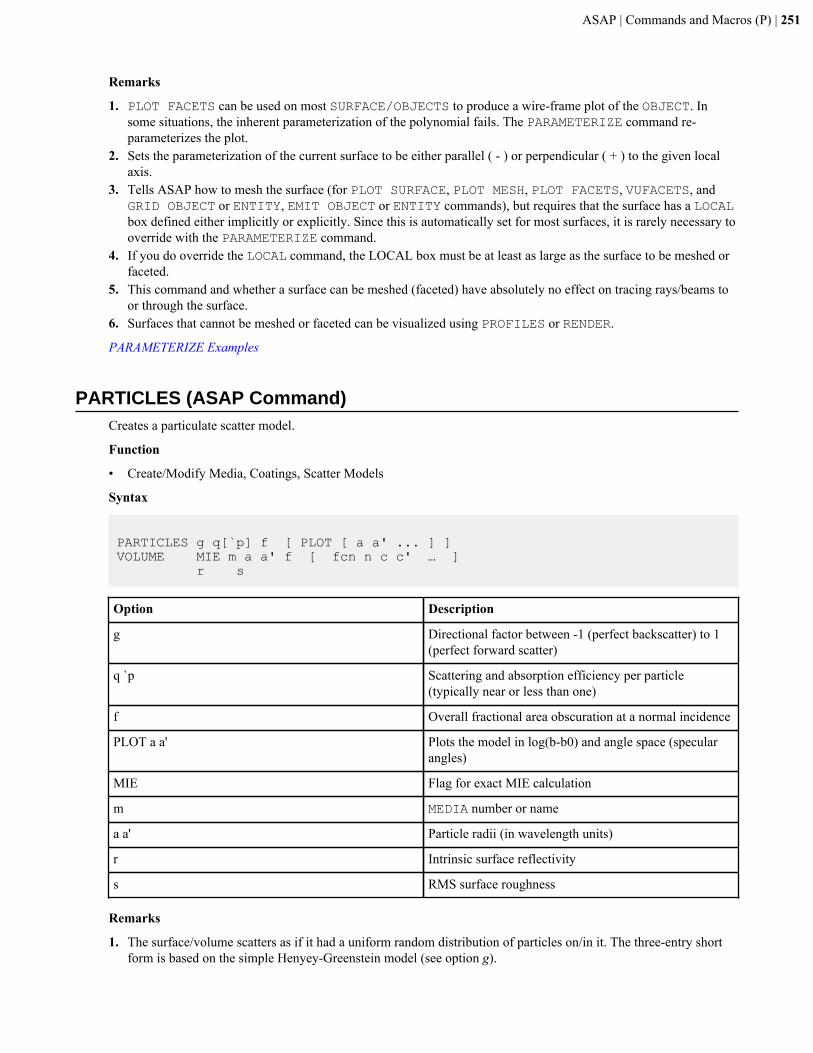
ASAP | Commands and Macros (P) | 251
Remarks
1. PLOT FACETS can be used on most SURFACE/OBJECTS to produce a wire-frame plot of the OBJECT. Insome situations, the inherent parameterization of the polynomial fails. The PARAMETERIZE command re-parameterizes the plot.
2. Sets the parameterization of the current surface to be either parallel ( - ) or perpendicular ( + ) to the given localaxis.
3. Tells ASAP how to mesh the surface (for PLOT SURFACE, PLOT MESH, PLOT FACETS, VUFACETS, andGRID OBJECT or ENTITY, EMIT OBJECT or ENTITY commands), but requires that the surface has a LOCALbox defined either implicitly or explicitly. Since this is automatically set for most surfaces, it is rarely necessary tooverride with the PARAMETERIZE command.
4. If you do override the LOCAL command, the LOCAL box must be at least as large as the surface to be meshed orfaceted.
5. This command and whether a surface can be meshed (faceted) have absolutely no effect on tracing rays/beams toor through the surface.
6. Surfaces that cannot be meshed or faceted can be visualized using PROFILES or RENDER.
PARAMETERIZE Examples
PARTICLES (ASAP Command)Creates a particulate scatter model.
Function
• Create/Modify Media, Coatings, Scatter Models
Syntax
PARTICLES g q[`p] f [ PLOT [ a a' ... ] ]VOLUME MIE m a a' f [ fcn n c c' … ] r s
Option Description
g Directional factor between -1 (perfect backscatter) to 1(perfect forward scatter)
q `p Scattering and absorption efficiency per particle(typically near or less than one)
f Overall fractional area obscuration at a normal incidence
PLOT a a' Plots the model in log(b-b0) and angle space (specularangles)
MIE Flag for exact MIE calculation
m MEDIA number or name
a a' Particle radii (in wavelength units)
r Intrinsic surface reflectivity
s RMS surface roughness
Remarks
1. The surface/volume scatters as if it had a uniform random distribution of particles on/in it. The three-entry shortform is based on the simple Henyey-Greenstein model (see option g).
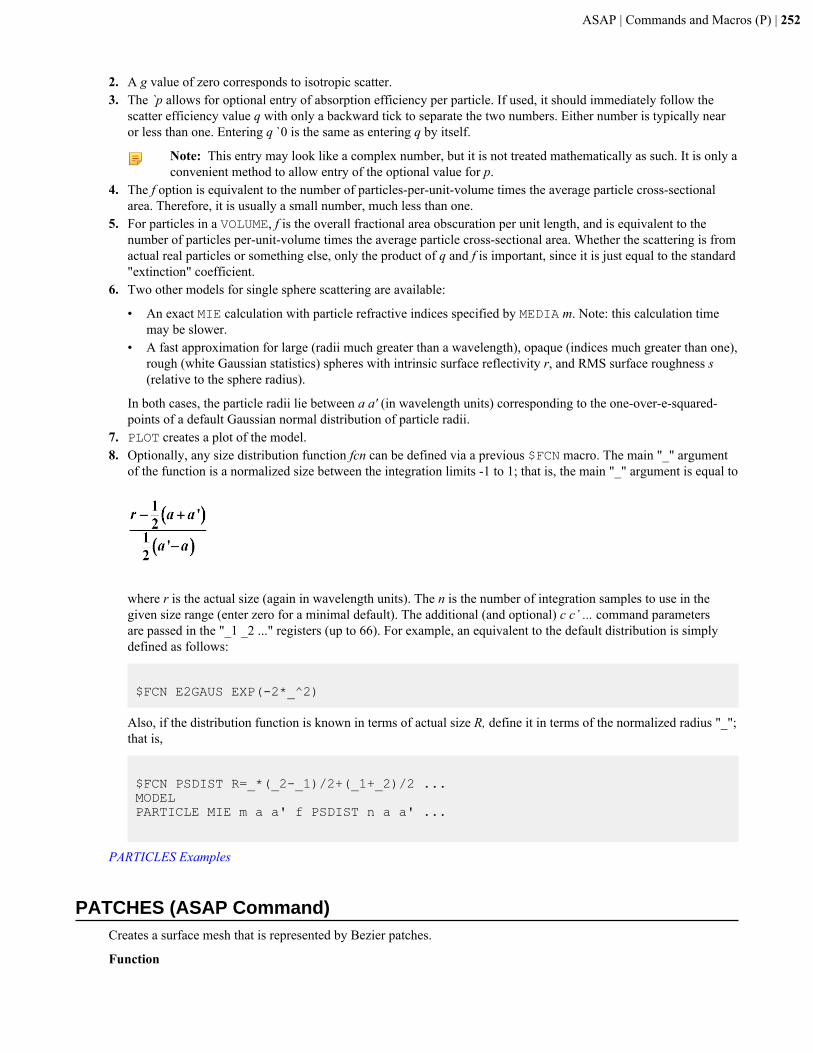
ASAP | Commands and Macros (P) | 252
2. A g value of zero corresponds to isotropic scatter.3. The `p allows for optional entry of absorption efficiency per particle. If used, it should immediately follow the
scatter efficiency value q with only a backward tick to separate the two numbers. Either number is typically nearor less than one. Entering q `0 is the same as entering q by itself.
Note: This entry may look like a complex number, but it is not treated mathematically as such. It is only aconvenient method to allow entry of the optional value for p.
4. The f option is equivalent to the number of particles-per-unit-volume times the average particle cross-sectionalarea. Therefore, it is usually a small number, much less than one.
5. For particles in a VOLUME, f is the overall fractional area obscuration per unit length, and is equivalent to thenumber of particles per-unit-volume times the average particle cross-sectional area. Whether the scattering is fromactual real particles or something else, only the product of q and f is important, since it is just equal to the standard"extinction" coefficient.
6. Two other models for single sphere scattering are available:
• An exact MIE calculation with particle refractive indices specified by MEDIA m. Note: this calculation timemay be slower.
• A fast approximation for large (radii much greater than a wavelength), opaque (indices much greater than one),rough (white Gaussian statistics) spheres with intrinsic surface reflectivity r, and RMS surface roughness s(relative to the sphere radius).
In both cases, the particle radii lie between a a' (in wavelength units) corresponding to the one-over-e-squared-points of a default Gaussian normal distribution of particle radii.
7. PLOT creates a plot of the model.8. Optionally, any size distribution function fcn can be defined via a previous $FCN macro. The main "_" argument
of the function is a normalized size between the integration limits -1 to 1; that is, the main "_" argument is equal to
where r is the actual size (again in wavelength units). The n is the number of integration samples to use in thegiven size range (enter zero for a minimal default). The additional (and optional) c c’ ... command parametersare passed in the "_1 _2 ..." registers (up to 66). For example, an equivalent to the default distribution is simplydefined as follows:
$FCN E2GAUS EXP(-2*_^2)
Also, if the distribution function is known in terms of actual size R, define it in terms of the normalized radius "_";that is,
$FCN PSDIST R=_*(_2-_1)/2+(_1+_2)/2 ...MODELPARTICLE MIE m a a' f PSDIST n a a' ...
PARTICLES Examples
PATCHES (ASAP Command)Creates a surface mesh that is represented by Bezier patches.
Function
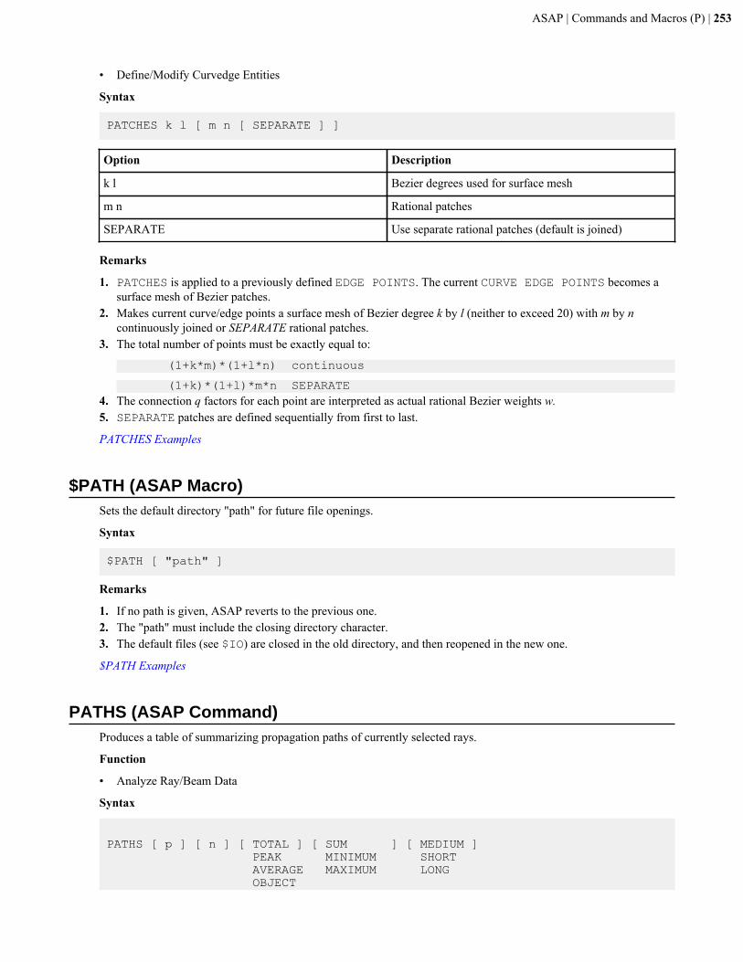
ASAP | Commands and Macros (P) | 253
• Define/Modify Curvedge Entities
Syntax
PATCHES k l [ m n [ SEPARATE ] ]
Option Description
k l Bezier degrees used for surface mesh
m n Rational patches
SEPARATE Use separate rational patches (default is joined)
Remarks
1. PATCHES is applied to a previously defined EDGE POINTS. The current CURVE EDGE POINTS becomes asurface mesh of Bezier patches.
2. Makes current curve/edge points a surface mesh of Bezier degree k by l (neither to exceed 20) with m by ncontinuously joined or SEPARATE rational patches.
3. The total number of points must be exactly equal to:
(1+k*m)*(1+l*n) continuous
(1+k)*(1+l)*m*n SEPARATE4. The connection q factors for each point are interpreted as actual rational Bezier weights w.5. SEPARATE patches are defined sequentially from first to last.
PATCHES Examples
$PATH (ASAP Macro)Sets the default directory "path" for future file openings.
Syntax
$PATH [ "path" ]
Remarks
1. If no path is given, ASAP reverts to the previous one.2. The "path" must include the closing directory character.3. The default files (see $IO) are closed in the old directory, and then reopened in the new one.
$PATH Examples
PATHS (ASAP Command)Produces a table of summarizing propagation paths of currently selected rays.
Function
• Analyze Ray/Beam Data
Syntax
PATHS [ p ] [ n ] [ TOTAL ] [ SUM ] [ MEDIUM ] PEAK MINIMUM SHORT AVERAGE MAXIMUM LONG OBJECT
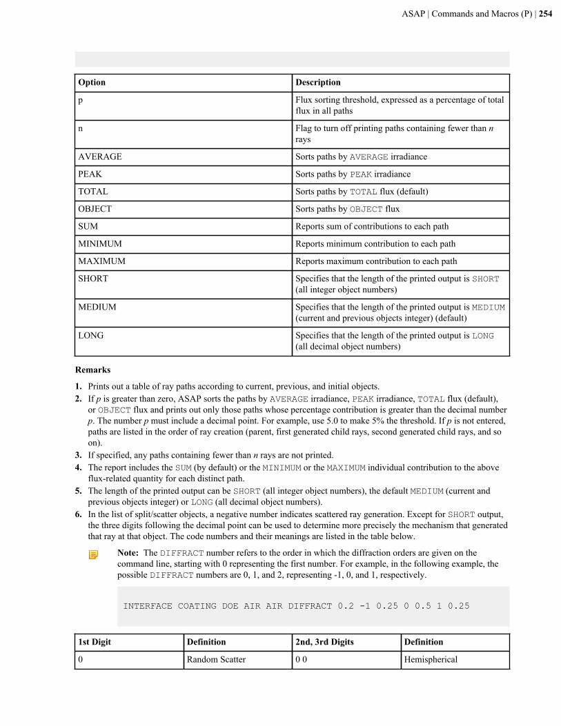
ASAP | Commands and Macros (P) | 254
Option Description
p Flux sorting threshold, expressed as a percentage of totalflux in all paths
n Flag to turn off printing paths containing fewer than nrays
AVERAGE Sorts paths by AVERAGE irradiance
PEAK Sorts paths by PEAK irradiance
TOTAL Sorts paths by TOTAL flux (default)
OBJECT Sorts paths by OBJECT flux
SUM Reports sum of contributions to each path
MINIMUM Reports minimum contribution to each path
MAXIMUM Reports maximum contribution to each path
SHORT Specifies that the length of the printed output is SHORT(all integer object numbers)
MEDIUM Specifies that the length of the printed output is MEDIUM(current and previous objects integer) (default)
LONG Specifies that the length of the printed output is LONG(all decimal object numbers)
Remarks
1. Prints out a table of ray paths according to current, previous, and initial objects.2. If p is greater than zero, ASAP sorts the paths by AVERAGE irradiance, PEAK irradiance, TOTAL flux (default),
or OBJECT flux and prints out only those paths whose percentage contribution is greater than the decimal numberp. The number p must include a decimal point. For example, use 5.0 to make 5% the threshold. If p is not entered,paths are listed in the order of ray creation (parent, first generated child rays, second generated child rays, and soon).
3. If specified, any paths containing fewer than n rays are not printed.4. The report includes the SUM (by default) or the MINIMUM or the MAXIMUM individual contribution to the above
flux-related quantity for each distinct path.5. The length of the printed output can be SHORT (all integer object numbers), the default MEDIUM (current and
previous objects integer) or LONG (all decimal object numbers).6. In the list of split/scatter objects, a negative number indicates scattered ray generation. Except for SHORT output,
the three digits following the decimal point can be used to determine more precisely the mechanism that generatedthat ray at that object. The code numbers and their meanings are listed in the table below.
Note: The DIFFRACT number refers to the order in which the diffraction orders are given on thecommand line, starting with 0 representing the first number. For example, in the following example, thepossible DIFFRACT numbers are 0, 1, and 2, representing -1, 0, and 1, respectively.
INTERFACE COATING DOE AIR AIR DIFFRACT 0.2 -1 0.25 0 0.5 1 0.25
1st Digit Definition 2nd, 3rd Digits Definition
0 Random Scatter 0 0 Hemispherical
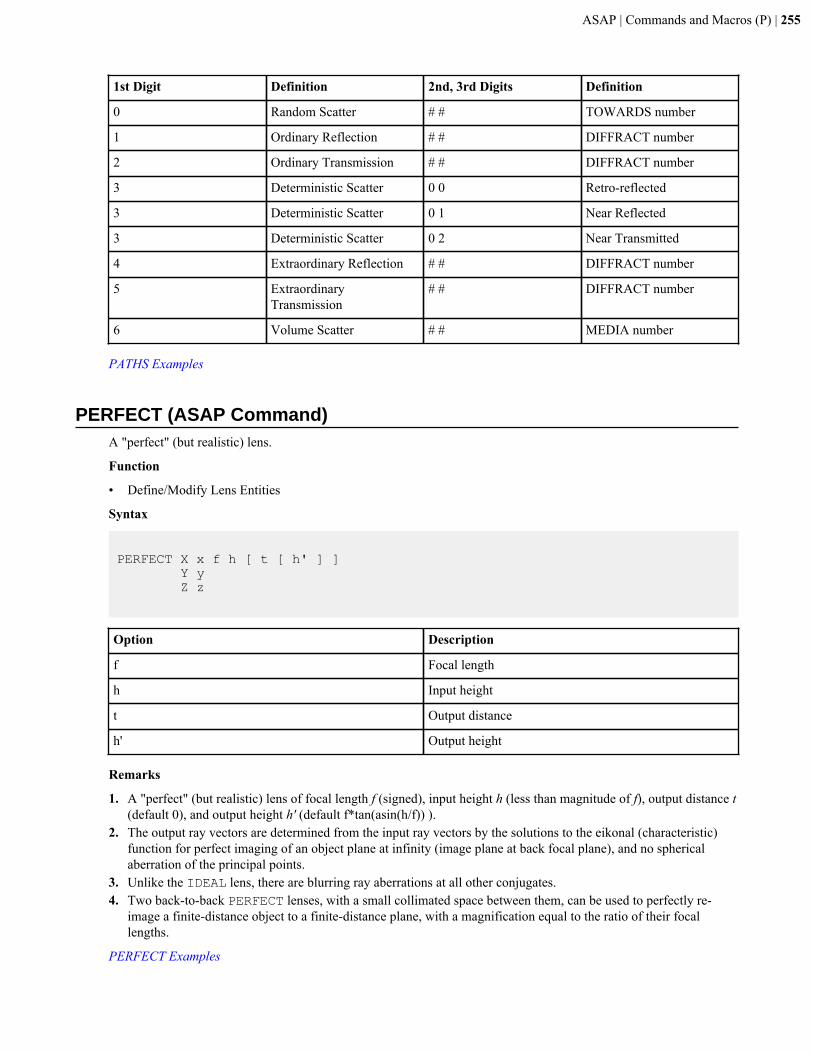
ASAP | Commands and Macros (P) | 255
1st Digit Definition 2nd, 3rd Digits Definition
0 Random Scatter # # TOWARDS number
1 Ordinary Reflection # # DIFFRACT number
2 Ordinary Transmission # # DIFFRACT number
3 Deterministic Scatter 0 0 Retro-reflected
3 Deterministic Scatter 0 1 Near Reflected
3 Deterministic Scatter 0 2 Near Transmitted
4 Extraordinary Reflection # # DIFFRACT number
5 ExtraordinaryTransmission
# # DIFFRACT number
6 Volume Scatter # # MEDIA number
PATHS Examples
PERFECT (ASAP Command)A "perfect" (but realistic) lens.
Function
• Define/Modify Lens Entities
Syntax
PERFECT X x f h [ t [ h' ] ] Y y Z z
Option Description
f Focal length
h Input height
t Output distance
h' Output height
Remarks
1. A "perfect" (but realistic) lens of focal length f (signed), input height h (less than magnitude of f), output distance t(default 0), and output height h' (default f*tan(asin(h/f)) ).
2. The output ray vectors are determined from the input ray vectors by the solutions to the eikonal (characteristic)function for perfect imaging of an object plane at infinity (image plane at back focal plane), and no sphericalaberration of the principal points.
3. Unlike the IDEAL lens, there are blurring ray aberrations at all other conjugates.4. Two back-to-back PERFECT lenses, with a small collimated space between them, can be used to perfectly re-
image a finite-distance object to a finite-distance plane, with a magnification equal to the ratio of their focallengths.
PERFECT Examples
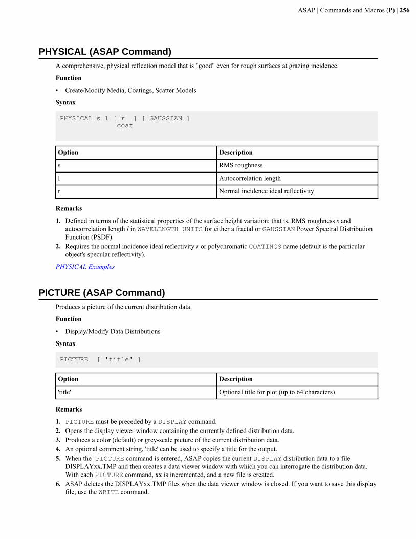
ASAP | Commands and Macros (P) | 256
PHYSICAL (ASAP Command)A comprehensive, physical reflection model that is "good" even for rough surfaces at grazing incidence.
Function
• Create/Modify Media, Coatings, Scatter Models
Syntax
PHYSICAL s l [ r ] [ GAUSSIAN ] coat
Option Description
s RMS roughness
l Autocorrelation length
r Normal incidence ideal reflectivity
Remarks
1. Defined in terms of the statistical properties of the surface height variation; that is, RMS roughness s andautocorrelation length l in WAVELENGTH UNITS for either a fractal or GAUSSIAN Power Spectral DistributionFunction (PSDF).
2. Requires the normal incidence ideal reflectivity r or polychromatic COATINGS name (default is the particularobject's specular reflectivity).
PHYSICAL Examples
PICTURE (ASAP Command)Produces a picture of the current distribution data.
Function
• Display/Modify Data Distributions
Syntax
PICTURE [ 'title' ]
Option Description
'title' Optional title for plot (up to 64 characters)
Remarks
1. PICTURE must be preceded by a DISPLAY command.2. Opens the display viewer window containing the currently defined distribution data.3. Produces a color (default) or grey-scale picture of the current distribution data.4. An optional comment string, 'title' can be used to specify a title for the output.5. When the PICTURE command is entered, ASAP copies the current DISPLAY distribution data to a file
DISPLAYxx.TMP and then creates a data viewer window with which you can interrogate the distribution data.With each PICTURE command, xx is incremented, and a new file is created.
6. ASAP deletes the DISPLAYxx.TMP files when the data viewer window is closed. If you want to save this displayfile, use the WRITE command.
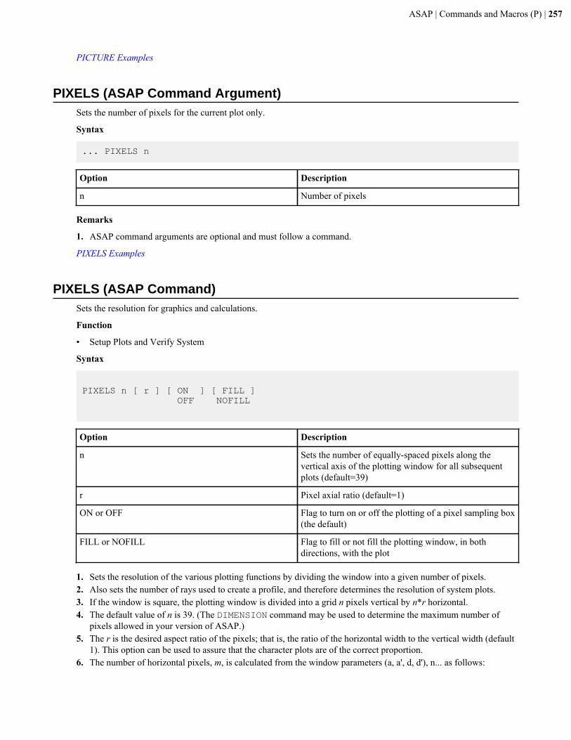
ASAP | Commands and Macros (P) | 257
PICTURE Examples
PIXELS (ASAP Command Argument)Sets the number of pixels for the current plot only.
Syntax
... PIXELS n
Option Description
n Number of pixels
Remarks
1. ASAP command arguments are optional and must follow a command.
PIXELS Examples
PIXELS (ASAP Command)Sets the resolution for graphics and calculations.
Function
• Setup Plots and Verify System
Syntax
PIXELS n [ r ] [ ON ] [ FILL ] OFF NOFILL
Option Description
n Sets the number of equally-spaced pixels along thevertical axis of the plotting window for all subsequentplots (default=39)
r Pixel axial ratio (default=1)
ON or OFF Flag to turn on or off the plotting of a pixel sampling box(the default)
FILL or NOFILL Flag to fill or not fill the plotting window, in bothdirections, with the plot
1. Sets the resolution of the various plotting functions by dividing the window into a given number of pixels.2. Also sets the number of rays used to create a profile, and therefore determines the resolution of system plots.3. If the window is square, the plotting window is divided into a grid n pixels vertical by n*r horizontal.4. The default value of n is 39. (The DIMENSION command may be used to determine the maximum number of
pixels allowed in your version of ASAP.)5. The r is the desired aspect ratio of the pixels; that is, the ratio of the horizontal width to the vertical width (default
1). This option can be used to assure that the character plots are of the correct proportion.6. The number of horizontal pixels, m, is calculated from the window parameters (a, a', d, d'), n... as follows:
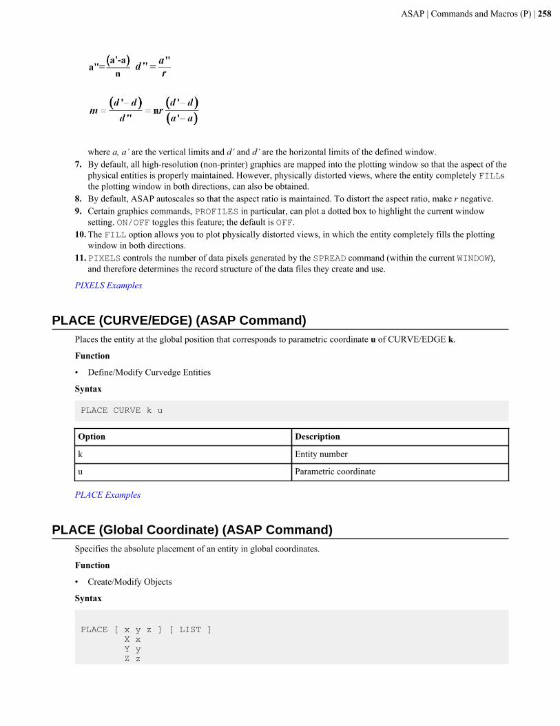
ASAP | Commands and Macros (P) | 258
where a, a’ are the vertical limits and d’ and d’ are the horizontal limits of the defined window.7. By default, all high-resolution (non-printer) graphics are mapped into the plotting window so that the aspect of the
physical entities is properly maintained. However, physically distorted views, where the entity completely FILLsthe plotting window in both directions, can also be obtained.
8. By default, ASAP autoscales so that the aspect ratio is maintained. To distort the aspect ratio, make r negative.9. Certain graphics commands, PROFILES in particular, can plot a dotted box to highlight the current window
setting. ON/OFF toggles this feature; the default is OFF.10. The FILL option allows you to plot physically distorted views, in which the entity completely fills the plotting
window in both directions.11.PIXELS controls the number of data pixels generated by the SPREAD command (within the current WINDOW),
and therefore determines the record structure of the data files they create and use.
PIXELS Examples
PLACE (CURVE/EDGE) (ASAP Command)Places the entity at the global position that corresponds to parametric coordinate u of CURVE/EDGE k.
Function
• Define/Modify Curvedge Entities
Syntax
PLACE CURVE k u
Option Description
k Entity number
u Parametric coordinate
PLACE Examples
PLACE (Global Coordinate) (ASAP Command)Specifies the absolute placement of an entity in global coordinates.
Function
• Create/Modify Objects
Syntax
PLACE [ x y z ] [ LIST ] X x Y y Z z
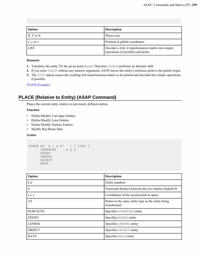
ASAP | Commands and Macros (P) | 259
Option Description
X, Y or Z Places axis
x, y or z Position in global coordinates
LIST Decodes a 4-by-4 transformation matrix into simpleoperations (if possible) and prints
Remarks
1. Translates the entity TO the given point (x,y,z). Therefore, PLACE performs an absolute shift.2. If you enter PLACE without any numeric arguments, ASAP moves the entity's reference point to the global origin.3. The LIST option causes the resulting 4x4 transformation matrix to be printed and decoded into simple operations,
if possible.
PLACE Examples
PLACE (Relative to Entity) (ASAP Command)Places the current entity relative to previously defined entities.
Function
• Define/Modify Curvedge Entities• Define/Modify Lens Entities• Define/Modify Surfunc Entities• Modify Ray/Beam Data
Syntax
PLACE AT k [ d k' ] [ LIST ] SURFACES x y z EDGES LENSES OBJECT RAYS
Option Description
k k' Entity numbers
d Fractional distance between the two entities (default 0)
x y z Coordinates of the second point in space
AT Refers to the same entity type as the entity beingtransformed
SURFACES Specifies SURFACES entity
EDGES Specifies EDGES entity
LENSES Specifies LENSES entity
OBJECT Specifies OBJECT entity
RAYS Specifies RAYS entity
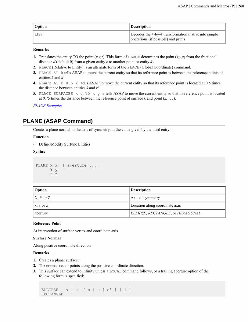
ASAP | Commands and Macros (P) | 260
Option Description
LIST Decodes the 4-by-4 transformation matrix into simpleoperations (if possible) and prints
Remarks
1. Translates the entity TO the point (x,y,z). This form of PLACE determines the point (x,y,z) from the fractionaldistance d (default 0) from a given entity k to another point or entity k'.
2. PLACE (Relative to Entity) is an alternate form of the PLACE (Global Coordinate) command.3. PLACE AT k tells ASAP to move the current entity so that its reference point is between the reference points of
entities k and k'4. PLACE AT k 0.5 k' tells ASAP to move the current entity so that its reference point is located at 0.5 times
the distance between entities k and k'.5. PLACE SURFACES k 0.75 x y z tells ASAP to move the current entity so that its reference point is located
at 0.75 times the distance between the reference point of surface k and point (x, y, z).
PLACE Examples
PLANE (ASAP Command)Creates a plane normal to the axis of symmetry, at the value given by the third entry.
Function
• Define/Modify Surfunc Entities
Syntax
PLANE X x [ aperture ... ] Y y Z z
Option Description
X, Y or Z Axis of symmetry
x, y or z Location along coordinate axis
aperture ELLIPSE, RECTANGLE, or HEXAGONAL
Reference Point
At intersection of surface vertex and coordinate axis
Surface Normal
Along positive coordinate direction
Remarks
1. Creates a planar surface.2. The normal vector points along the positive coordinate direction.3. This surface can extend to infinity unless a LOCAL command follows, or a trailing aperture option of the
following form is specified:
ELLIPSE a [ a' [ o [ s [ s' ] ] ] ]RECTANGLE
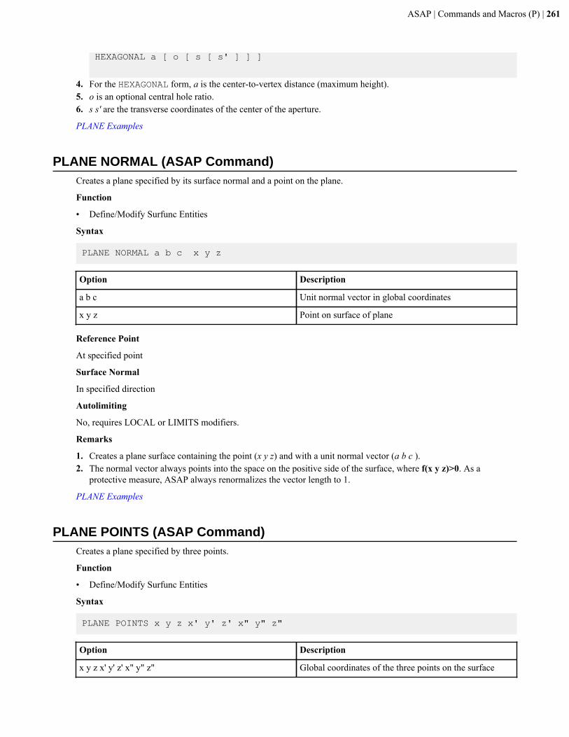
ASAP | Commands and Macros (P) | 261
HEXAGONAL a [ o [ s [ s' ] ] ]
4. For the HEXAGONAL form, a is the center-to-vertex distance (maximum height).5. o is an optional central hole ratio.6. s s' are the transverse coordinates of the center of the aperture.
PLANE Examples
PLANE NORMAL (ASAP Command)Creates a plane specified by its surface normal and a point on the plane.
Function
• Define/Modify Surfunc Entities
Syntax
PLANE NORMAL a b c x y z
Option Description
a b c Unit normal vector in global coordinates
x y z Point on surface of plane
Reference Point
At specified point
Surface Normal
In specified direction
Autolimiting
No, requires LOCAL or LIMITS modifiers.
Remarks
1. Creates a plane surface containing the point (x y z) and with a unit normal vector (a b c ).2. The normal vector always points into the space on the positive side of the surface, where f(x y z)>0. As a
protective measure, ASAP always renormalizes the vector length to 1.
PLANE Examples
PLANE POINTS (ASAP Command)Creates a plane specified by three points.
Function
• Define/Modify Surfunc Entities
Syntax
PLANE POINTS x y z x' y' z' x" y" z"
Option Description
x y z x' y' z' x" y" z" Global coordinates of the three points on the surface
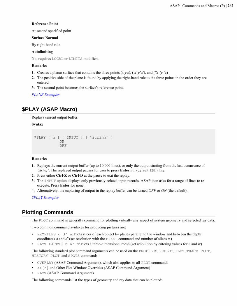
ASAP | Commands and Macros (P) | 262
Reference Point
At second specified point
Surface Normal
By right-hand rule
Autolimiting
No, requires LOCAL or LIMITS modifiers.
Remarks
1. Creates a planar surface that contains the three points (x y z), ( x' y' z'), and ("x "y "z)2. The positive side of the plane is found by applying the right-hand rule to the three points in the order they are
entered.3. The second point becomes the surface's reference point.
PLANE Examples
$PLAY (ASAP Macro)Replays current output buffer.
Syntax
$PLAY [ n ] [ INPUT ] [ ’string’ ] ON OFF
Remarks
1. Replays the current output buffer (up to 10,000 lines), or only the output starting from the last occurrence of’string’. The replayed output pauses for user to press Enter nth (default 12th) line.
2. Press either Ctrl-Z or Ctrl-D at the pause to exit the replay.3. The INPUT option displays only previously echoed input records. ASAP then asks for a range of lines to re-
execute. Press Enter for none.4. Alternatively, the capturing of output in the replay buffer can be turned OFF or ON (the default).
$PLAY Examples
Plotting CommandsThe PLOT command is generally command for plotting virtually any aspect of system geometry and selected ray data.
Two common command syntaxes for producing pictures are:
• PROFILES d d' n: Plots slices of each object by planes parallel to the window and between the depthcoordinates d and d' (set resolution with the PIXEL command and number of slices n.)
• PLOT FACETS n n' m: Plots a three-dimensional mesh (set resolution by entering values for n and n').
The following standard plot command arguments can be used on the PROFILES, REPLOT, PLOT, TRACE PLOT,HISTORY PLOT, and SPOTS commands:
• OVERLAY (ASAP Command Argument), which also applies to all PLOT commands• XY[Z] and Other Plot Window Overrides (ASAP Command Argument)• PLOT (ASAP Command Argument).
The following commands list the types of geometry and ray data that can be plotted:
ASAP | Commands and Macros (P) | 263
• PLOT3D• PLOT CURVES• PLOT BEAMS• PLOT EDGES• PLOT ENTITIES• PLOT FACETS• PLOT LENSES• PLOT LIMITS• PLOT LOCAL• PLOT MESHES• PLOT POLARIZATION• PLOT RAYS• PLOT SURFACES
PLOT3D (ASAP Command)Creates a 3D representation of the current distribution data file with 1D cross-sections.
Function
• Display/Modify Data Distributions
Syntax
PLOT3D [ s ] [ t [ r ] ]
Option Description
s Readjusts the vertical scale
t Tilt (default 18)
r Rotation (default 33)
Remarks
1. Produces a 3D hidden line representation of the data and a set of 1D cross-sections on the same plot.2. The s can be used to readjust the vertical scale of the plot downward (that is, s less than 1).3. The actual view is controlled by the tilt t and rotation r angles in degrees (defaults 18 and 33). Both these angles
should be greather than 1.5 degrees and less than 90.4. The OVERLAY command argument tells ASAP not to issue an end of plot so that the next plot created is overlaid
with the current plot. This is useful for combining system plots with ray trace plots (assuming that the WINDOW isthe same for all plots), multiple spot diagrams, and so on.
PLOT3D Examples
PLOT BEAMS (ASAP Command)Plots extent of each Gaussian beam within the currently specified graphics window.
Function
• Analyze Ray/Beam Data
Syntax
PLOT BEAMS [ 'title' ]
ASAP | Commands and Macros (P) | 264
Option Description
'title' Optional title for plot (up to 64 characters); delimited bysingle quotes
Remarks
1. Plots either existing parabasal ray data or internally generated, symmetric, Gaussian ray data within the windowspecified by the WINDOW command. The half-amplitude ellipses are plotted.
2. May be executed at any time after the beam is constructed. Use the WINDOW command to set the plotting window.3. WINDOW, WINDOW X Z, WINDOW Y X, and WINDOW Z Y display the system in a left-handed coordinate
system. Use WINDOW X -Z, WINDOW Y -X, or WINDOW Z -Y to display the system in a right-handedcoordinate system.
4. Use the SELECT and CONSIDER commands to restrict either the ray set or the objects.5. In addition to the 2D plot that is generated, the full 3D data is written to the VECTOR (*.vcr) file (default logical
unit 30).6. The OVERLAY command argument tells ASAP not to issue an end of plot so that the next plot created is overlaid
with the current plot. This is useful for combining system plots with ray trace plots (assuming that the WINDOW isthe same for all plots), multiple spot diagrams, and so on.
PLOT Examples
PLOT CURVES (ASAP Command)Plots a wire-frame outline of curves, with the control points displayed, in the currently specified graphics window.
Function
• Setup Plots and Verify System
Syntax
PLOT CURVES [ -n ] [ 'title' ] [ k [ k' [ k" ] ] ]
Option Description
n Plot last n curves
k k' k" Range of edges (k to k') to be plotted in "k steps
'title' Optional title for plot (up to 64 characters); delimited bysingle quotes
Remarks
1. By default, plots all currently defined curves, whether or not they are assigned to objects.2. If n is negative, the last n curves are plotted.3. If k is positive and no other entries are present, only the kth curves is plotted.4. If k and k' are present, curves k through k' are plotted.5. If k, k', and "k are all present, ASAP plots curves k through k' in steps of "k (that is, PLOT CURVES 1 5 2 tells
ASAP to plot curves 1, 3, and 5).6. WINDOW, WINDOW X Z, WINDOW Y X, and WINDOW Z Y display the system in a left-handed coordinate
system. Use WINDOW X -Z, WINDOW Y -X, or WINDOW Z -Y to display the system in a right-handedcoordinate system.
ASAP | Commands and Macros (P) | 265
7. In addition to the 2D plot that is generated, the full 3D data is written to the VECTOR file (default logical unit30).
8. The OVERLAY command argument instructs ASAP not to issue an end of plot so that the next plot created isoverlaid with the current plot. This is useful for combining system plots with ray trace plots (assuming that theWINDOW is the same for all plots), multiple spot diagrams, and so on.
PLOT Examples
PLOT EDGES (ASAP Command)Plots a wireframe outline of edges in the currently specified graphics window.
Function
• Setup Plots and Verify System
Syntax
PLOT EDGES [ -n ] [ 'title' ] [ k [ k' [ k" ] ] ]
Option Description
n Plot last n edges
k k' k" Range of edges (k to k') to be plotted in "k steps
'title' Optional title for plot (up to 64 characters); delimited bysingle quotes
Remarks
1. By default, plots all currently defined edges, whether or not they are assigned to objects.2. If n is negative, the last n edges are plotted.3. If k is positive and no other entries are present, only the kth edge is plotted.4. If k and k' are present, edges k through k' are plotted.5. If k, k', and "k are all present, ASAP plots edges k through k' in steps of "k (that is, PLOT EDGES 1 5 2 tells
ASAP to plot edges 1, 3, and 5).6. WINDOW, WINDOW X Z, WINDOW Y X, and WINDOW Z Y display the system in a left-handed coordinate
system. Use WINDOW X -Z, WINDOW Y -X, or WINDOW Z -Y to display the system in a right-handedcoordinate system.
7. In addition to the 2D plot that is generated, the full 3D data is written to the VECTOR file (default logical unit30).
8. The OVERLAY command argument tells ASAP not to issue an end of plot, so that the next plot created is overlaidwith the current plot. This is useful for combining system plots with ray trace plots (assuming that the WINDOW isthe same for all plots), multiple spot diagrams, and so on.
PLOT Examples
PLOT ENTITIES (ASAP Command)Plots surface, edge, and lens entities in the currently specified graphics window.
Function
• Setup Plots and Verify System
ASAP | Commands and Macros (P) | 266
Syntax
PLOT ENTITIES [ -n ] [ 'title' ] [ k [ k' [ k" ] ] ]
Option Description
n Plot last n entities
k k' k" Range of edges (k to k') to be plotted in "k steps
'title' Optional title for plot (up to 64 characters); delimited bysingle quotes
Remarks
1. By default, plots all currently defined surface, edge, and lens entities, whether or not they are assigned to objects.2. If n is negative, the last n entities are plotted.3. If k is positive and no other entries are present, only the kth entity is plotted.4. If k and k' are entered, entities k through k' are plotted.5. If k, k', and "k are all present, ASAP plots entities k through k' in steps of "k (that is, PLOT ENTITIES 1 5 2
tells ASAP to plot entities 1, 3, and 5).6. WINDOW, WINDOW X Z, WINDOW Y X, and WINDOW Z Y display the system in a left-handed coordinate
system. Use WINDOW X -Z, WINDOW Y -X, or WINDOW Z -Y to display the system in a right-handedcoordinate system.
7. In addition to the 2D plot that is generated, the full 3D data is written to the VECTOR file (default logical unit30).
8. The OVERLAY command argument tells ASAP not to issue an end of plot so that the next plot created is overlaidwith the current plot. This is useful for combining system plots with ray trace plots (assuming that the WINDOW isthe same for all plots), multiple spot diagrams, and so on.
PLOT Examples
PLOT FACETS (ASAP Command)Plots parametric mesh representation of objects in the currently specified graphics window.
Function
• Setup Plots and Verify System
Syntax 1
PLOT FACETS [ n n' [ m ] ] [ REMOVE ] [ 'title' ] HIDE [ d ]
Syntax 2
PLOT FACETS n m [MICROSTRUCTURE nc mc|AXIS]
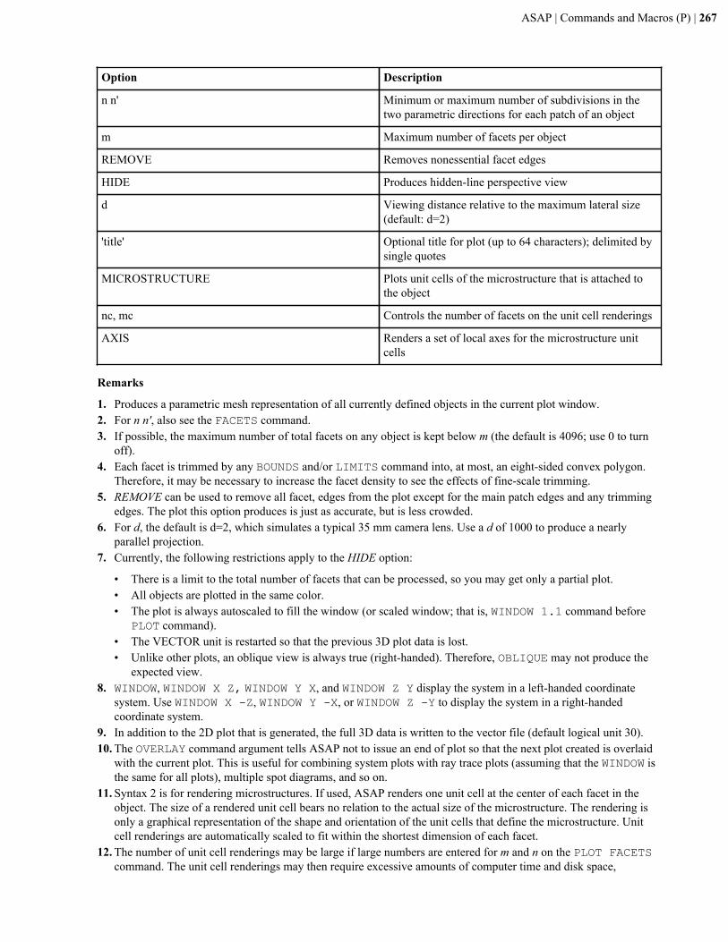
ASAP | Commands and Macros (P) | 267
Option Description
n n' Minimum or maximum number of subdivisions in thetwo parametric directions for each patch of an object
m Maximum number of facets per object
REMOVE Removes nonessential facet edges
HIDE Produces hidden-line perspective view
d Viewing distance relative to the maximum lateral size(default: d=2)
'title' Optional title for plot (up to 64 characters); delimited bysingle quotes
MICROSTRUCTURE Plots unit cells of the microstructure that is attached tothe object
nc, mc Controls the number of facets on the unit cell renderings
AXIS Renders a set of local axes for the microstructure unitcells
Remarks
1. Produces a parametric mesh representation of all currently defined objects in the current plot window.2. For n n', also see the FACETS command.3. If possible, the maximum number of total facets on any object is kept below m (the default is 4096; use 0 to turn
off).4. Each facet is trimmed by any BOUNDS and/or LIMITS command into, at most, an eight-sided convex polygon.
Therefore, it may be necessary to increase the facet density to see the effects of fine-scale trimming.5. REMOVE can be used to remove all facet, edges from the plot except for the main patch edges and any trimming
edges. The plot this option produces is just as accurate, but is less crowded.6. For d, the default is d=2, which simulates a typical 35 mm camera lens. Use a d of 1000 to produce a nearly
parallel projection.7. Currently, the following restrictions apply to the HIDE option:
• There is a limit to the total number of facets that can be processed, so you may get only a partial plot.• All objects are plotted in the same color.• The plot is always autoscaled to fill the window (or scaled window; that is, WINDOW 1.1 command before
PLOT command).• The VECTOR unit is restarted so that the previous 3D plot data is lost.• Unlike other plots, an oblique view is always true (right-handed). Therefore, OBLIQUE may not produce the
expected view.8. WINDOW, WINDOW X Z, WINDOW Y X, and WINDOW Z Y display the system in a left-handed coordinate
system. Use WINDOW X -Z, WINDOW Y -X, or WINDOW Z -Y to display the system in a right-handedcoordinate system.
9. In addition to the 2D plot that is generated, the full 3D data is written to the vector file (default logical unit 30).10. The OVERLAY command argument tells ASAP not to issue an end of plot so that the next plot created is overlaid
with the current plot. This is useful for combining system plots with ray trace plots (assuming that the WINDOW isthe same for all plots), multiple spot diagrams, and so on.
11. Syntax 2 is for rendering microstructures. If used, ASAP renders one unit cell at the center of each facet in theobject. The size of a rendered unit cell bears no relation to the actual size of the microstructure. The rendering isonly a graphical representation of the shape and orientation of the unit cells that define the microstructure. Unitcell renderings are automatically scaled to fit within the shortest dimension of each facet.
12. The number of unit cell renderings may be large if large numbers are entered for m and n on the PLOT FACETScommand. The unit cell renderings may then require excessive amounts of computer time and disk space,
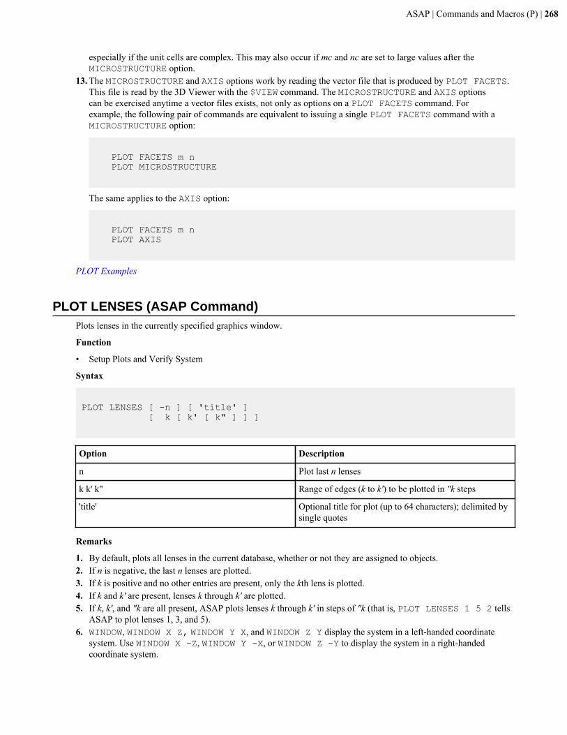
ASAP | Commands and Macros (P) | 268
especially if the unit cells are complex. This may also occur if mc and nc are set to large values after theMICROSTRUCTURE option.
13. The MICROSTRUCTURE and AXIS options work by reading the vector file that is produced by PLOT FACETS.This file is read by the 3D Viewer with the $VIEW command. The MICROSTRUCTURE and AXIS optionscan be exercised anytime a vector files exists, not only as options on a PLOT FACETS command. Forexample, the following pair of commands are equivalent to issuing a single PLOT FACETS command with aMICROSTRUCTURE option:
PLOT FACETS m n PLOT MICROSTRUCTURE
The same applies to the AXIS option:
PLOT FACETS m n PLOT AXIS
PLOT Examples
PLOT LENSES (ASAP Command)Plots lenses in the currently specified graphics window.
Function
• Setup Plots and Verify System
Syntax
PLOT LENSES [ -n ] [ 'title' ] [ k [ k' [ k" ] ] ]
Option Description
n Plot last n lenses
k k' k" Range of edges (k to k') to be plotted in "k steps
'title' Optional title for plot (up to 64 characters); delimited bysingle quotes
Remarks
1. By default, plots all lenses in the current database, whether or not they are assigned to objects.2. If n is negative, the last n lenses are plotted.3. If k is positive and no other entries are present, only the kth lens is plotted.4. If k and k' are present, lenses k through k' are plotted.5. If k, k', and "k are all present, ASAP plots lenses k through k' in steps of "k (that is, PLOT LENSES 1 5 2 tells
ASAP to plot lenses 1, 3, and 5).6. WINDOW, WINDOW X Z, WINDOW Y X, and WINDOW Z Y display the system in a left-handed coordinate
system. Use WINDOW X -Z, WINDOW Y -X, or WINDOW Z -Y to display the system in a right-handedcoordinate system.
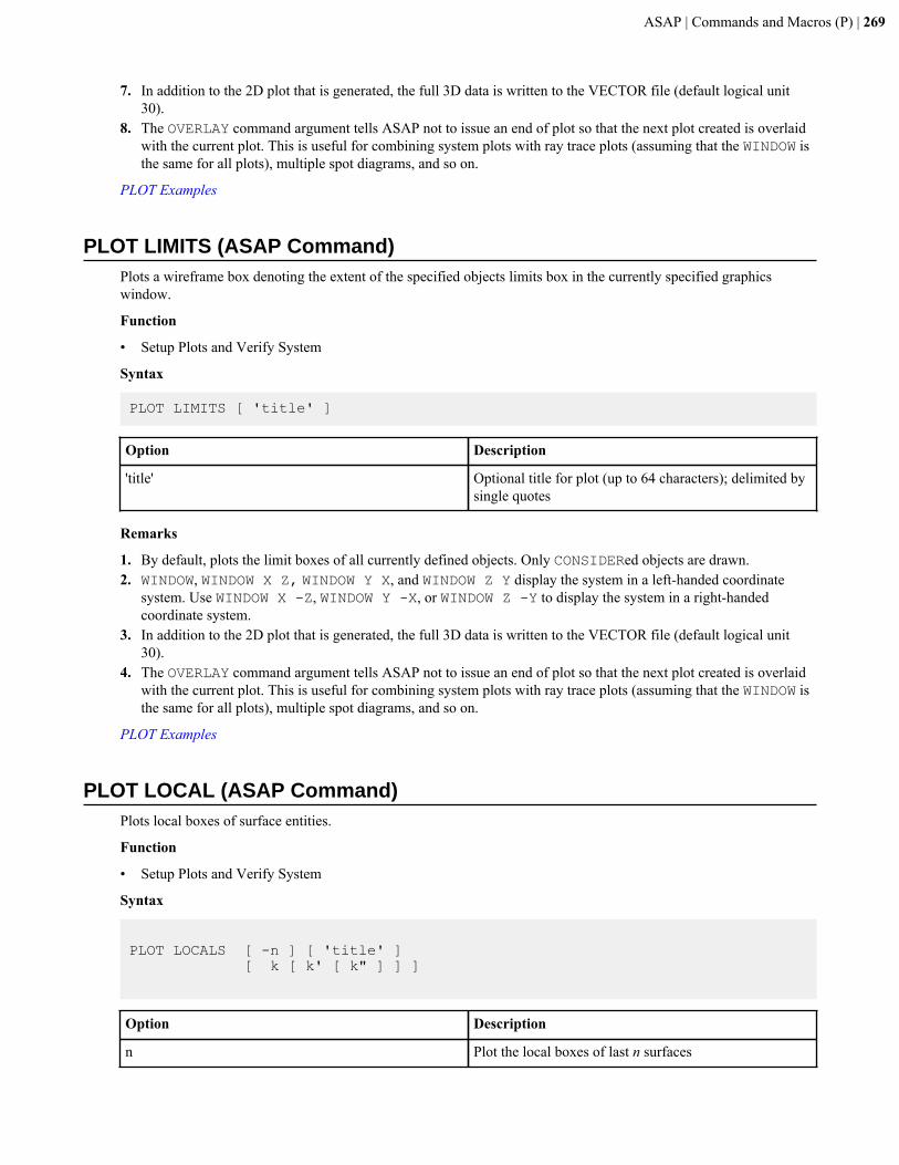
ASAP | Commands and Macros (P) | 269
7. In addition to the 2D plot that is generated, the full 3D data is written to the VECTOR file (default logical unit30).
8. The OVERLAY command argument tells ASAP not to issue an end of plot so that the next plot created is overlaidwith the current plot. This is useful for combining system plots with ray trace plots (assuming that the WINDOW isthe same for all plots), multiple spot diagrams, and so on.
PLOT Examples
PLOT LIMITS (ASAP Command)Plots a wireframe box denoting the extent of the specified objects limits box in the currently specified graphicswindow.
Function
• Setup Plots and Verify System
Syntax
PLOT LIMITS [ 'title' ]
Option Description
'title' Optional title for plot (up to 64 characters); delimited bysingle quotes
Remarks
1. By default, plots the limit boxes of all currently defined objects. Only CONSIDERed objects are drawn.2. WINDOW, WINDOW X Z, WINDOW Y X, and WINDOW Z Y display the system in a left-handed coordinate
system. Use WINDOW X -Z, WINDOW Y -X, or WINDOW Z -Y to display the system in a right-handedcoordinate system.
3. In addition to the 2D plot that is generated, the full 3D data is written to the VECTOR file (default logical unit30).
4. The OVERLAY command argument tells ASAP not to issue an end of plot so that the next plot created is overlaidwith the current plot. This is useful for combining system plots with ray trace plots (assuming that the WINDOW isthe same for all plots), multiple spot diagrams, and so on.
PLOT Examples
PLOT LOCAL (ASAP Command)Plots local boxes of surface entities.
Function
• Setup Plots and Verify System
Syntax
PLOT LOCALS [ -n ] [ 'title' ] [ k [ k' [ k" ] ] ]
Option Description
n Plot the local boxes of last n surfaces
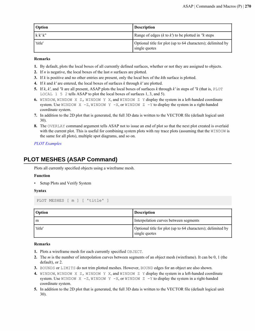
ASAP | Commands and Macros (P) | 270
Option Description
k k' k" Range of edges (k to k') to be plotted in "k steps
'title' Optional title for plot (up to 64 characters); delimited bysingle quotes
Remarks
1. By default, plots the local boxes of all currently defined surfaces, whether or not they are assigned to objects.2. If n is negative, the local boxes of the last n surfaces are plotted.3. If k is positive and no other entries are present, only the local box of the kth surface is plotted.4. If k and k' are entered, the local boxes of surfaces k through k' are plotted.5. If k, k', and "k are all present, ASAP plots the local boxes of surfaces k through k' in steps of "k (that is, PLOT
LOCAL 1 5 2 tells ASAP to plot the local boxes of surfaces 1, 3, and 5).6. WINDOW, WINDOW X Z, WINDOW Y X, and WINDOW Z Y display the system in a left-handed coordinate
system. Use WINDOW X -Z, WINDOW Y -X, or WINDOW Z -Y to display the system in a right-handedcoordinate system.
7. In addition to the 2D plot that is generated, the full 3D data is written to the VECTOR file (default logical unit30).
8. The OVERLAY command argument tells ASAP not to issue an end of plot so that the next plot created is overlaidwith the current plot. This is useful for combining system plots with ray trace plots (assuming that the WINDOW isthe same for all plots), multiple spot diagrams, and so on.
PLOT Examples
PLOT MESHES (ASAP Command)Plots all currently specified objects using a wireframe mesh.
Function
• Setup Plots and Verify System
Syntax
PLOT MESHES [ m ] [ 'title' ]
Option Description
m Interpolation curves between segments
'title' Optional title for plot (up to 64 characters); delimited bysingle quotes
Remarks
1. Plots a wireframe mesh for each currently specified OBJECT.2. The m is the number of interpolation curves between segments of an object mesh (wireframe). It can be 0, 1 (the
default), or 2.3. BOUNDS or LIMITS do not trim plotted meshes. However, BOUND edges for an object are also shown.4. WINDOW, WINDOW X Z, WINDOW Y X, and WINDOW Z Y display the system in a left-handed coordinate
system. Use WINDOW X -Z, WINDOW Y -X, or WINDOW Z -Y to display the system in a right-handedcoordinate system.
5. In addition to the 2D plot that is generated, the full 3D data is written to the VECTOR file (default logical unit30).
ASAP | Commands and Macros (P) | 271
6. The OVERLAY command argument tells ASAP not to issue an end of plot so that the next plot created is overlaidwith the current plot. This is useful for combining system plots with ray trace plots (assuming that the WINDOW isthe same for all plots), multiple spot diagrams, and so on.
PLOT Examples
PLOT POLARIZATION (ASAP Command)Plots polarization state ellipses.
Function
• Create Rays and Beams• Analyze Ray/Beam Data
Syntax
PLOT POLARIZATION [ e ] [ 'title' ]
Option Description
e Size of the ellipses is proportional to the ray/beam's fluxraised to the "e" power.
'title' Optional title for plot (up to 64 characters); delimited bysingle quotes
Remarks
CAUTION: The SOURCE propagation direction must be initialized before running PLOT POLARIZATION, or thecommand does not plot anything.
1. The polarization state ellipses for each ray/beam are plotted. The size of the ellipses is proportional to the ray/beam's flux raised to the e (default 1) power.
2. Arrows are drawn to show the handedness of the polarization state. In the case of linear polarization, arrows aredrawn on both ends of the degenerate ellipse. The size of the tip of the arrow used to show the handedness of thepolarization is determined by the overall size of the polarization ellipse. At times it might be necessary to use theARROW command to scale the tip for better visibility.
3. In Jones vector mode, PLOT POLARIZATION e, when e is less than 0, invokes the Poincare SphereVisualization Tool (PSVT) to visualize the polarization state in forms of Stokes vector. In Stokes vector mode,PLOT POLARIZATION always uses the PSVT to visualize the polarization state.
4. May be executed at any time after the beam is constructed.5. WINDOW, WINDOW X Z, WINDOW Y X, and WINDOW Z Y display the system in a left-handed coordinate
system. Use WINDOW X -Z, WINDOW Y -X, or WINDOW Z -Y to display the system in a right-handedcoordinate system.
6. In addition to the 2D plot that is generated, the full 3D data is written to the VECTOR file (default logical unit30).
7. The OVERLAY command argument tells ASAP not to issue an end of plot so that the next plot created is overlaidwith the current plot. This is useful for combining system plots with ray trace plots (assuming that the WINDOW isthe same for all plots), multiple spot diagrams, and so on.
PLOT Examples
ASAP | Commands and Macros (P) | 272
PLOT RAYS (ASAP Command)Plots vectors along the direction of each ray that is contained within the currently specified graphics window.
Function
• Analyze Ray/Beam Data
Syntax
PLOT RAYS d [ i ] [ 'title' ]
Option Description
d Scale factor for ray plot vector
i Plot only every ith ray
'title' Optional title for plot (up to 64 characters); delimited bysingle quotes
Remarks
1. Plots a line from the current position of each ray along its direction vector. The actual distance plotted is d timesthe flux of the ray divided by the maximum ray flux.
2. If d is entered as a negative number, only the endpoint of this vector is plotted. This structure is useful forproducing 3D far-field intensity distribution point clouds if d is much larger than any inter-ray distance. Thedefault for d is approximately 1/10th the window size.
3. WINDOW, WINDOW X Z, WINDOW Y X, and WINDOW Z Y display the system in a left-handed coordinatesystem. Use WINDOW X -Z, WINDOW Y -X, or WINDOW Z -Y to display the system in a right-handedcoordinate system.
4. In addition to the 2D plot that is generated, the full 3D data is written to the VECTOR file (default logical unit30).
5. The OVERLAY command argument tells ASAP not to issue an end of plot so that the next plot created is overlaidwith the current plot. This is useful for combining system plots with ray trace plots (assuming that the WINDOW isthe same for all plots), multiple spot diagrams, and so on.
PLOT RAYS Examples
PLOT SURFACES (ASAP Command)Plots surfaces in the currently specified graphics window.
Function
• Trace Rays/Beams
Syntax
PLOT SURFACES [ -n ] [ 'title' ] [ k [ k' [ k" ] ] ]
Option Description
n Plot last n surfaces
k k' k" Range of edges (k to k') to be plotted in "k steps
ASAP | Commands and Macros (P) | 273
Option Description
'title' Optional title for plot (up to 64 characters); delimited bysingle quotes
Remarks
1. By default, plots all currently defined surfaces, whether or not they are assigned to objects.2. If n is negative, the last n surfaces are plotted.3. If k is positive and no other entries are present, only the kth surface is plotted.4. If k and k' are entered, surfaces k through k' are plotted.5. If k, k', and "k are all present, ASAP plots surfaces k through k' in steps of "k (that is, PLOT SURFACES 1 5 2
tells ASAP to plot surfaces 1, 3, and 5).6. WINDOW, WINDOW X Z, WINDOW Y X, and WINDOW Z Y display the system in a left-handed coordinate
system. Use WINDOW X -Z, WINDOW Y -X, or WINDOW Z -Y to display the system in a right-handedcoordinate system.
7. In addition to the 2D plot that is generated, the full 3D data is written to the VECTOR file (default logical unit30).
8. The OVERLAY command argument tells ASAP not to issue an end of plot so that the next plot created is overlaidwith the current plot. This is useful for combining system plots with ray trace plots (assuming that the WINDOW isthe same for all plots), multiple spot diagrams, and so on.
PLOT Examples
PLOT (ASAP Command Argument)Plots the current model.
Syntax
... [ PLOT [ a a' ... ] [ OVERLAY ] ]
Option Description
a a' Specular angles
Remarks
1. ASAP command arguments are optional and must follow a command.2. Plots the model's BSDF for up to seven specular angles in ascending order (default 0, 15, 30, 45, 60, 75, 89.9
degrees).3. The current PIXELS setting controls the resolution of these plots in direction cosine space.4. For the default angles and a model sharply peaked at specular, the optimum setting for PIXELS is 580.5. Optionally, the multiple graphs plotted can be OVERLAYed into separate quadrants. If the angles a a' … are
explicitly given, PLOT also creates a full-hemispherical 2D distribution file, "name_angle.DIS", for each of thespecular angles.
6. Otherwise, the command argument, PLOT creates a 3D distribution file, name.dis, for each of these angles.7. Use command argument, OVERLAY to plot multiple graphs into separate quadrants.8. Assumes a unit reflectivity surface in the current IMMERSE media and at the current WAVELENGTH when a model
is plotted.
PLOT Examples
ASAP | Commands and Macros (P) | 274
$PLOT (ASAP Macro)Used to control screen graphics and plots.
Syntax
$PLOT [ OFF ] ASK EACH NORM
Option Description
OFF Suppresses screen graphics
ASK Prompts at end of each screen for plotting and/or saving
EACH Plots each screen without prompting
NORM Restores default (screen graphics and no prompting)
$PLOT Examples
POINTS (2D) (ASAP Command)Creates a generalized planar edge.
Function
• Define/Modify Curvedge Entities• Define/Modify Surfunc Entities
Syntax
POINTS X x y z q [ y' z' q' ... ] ABS REL Y y z x z' x' Z z x y x' y' :
Option Description
X, Y or Z Specifies coordinate axis
x, y or z Specifies location along coordinate axis
y z (z x or x y), y' z' ... Coordinates of point in orthogonal axes
q q' ... Connection parameters
ABS Measure all points in the global coordinate system
REL Measure all points RELative to the reference point
Reference Point
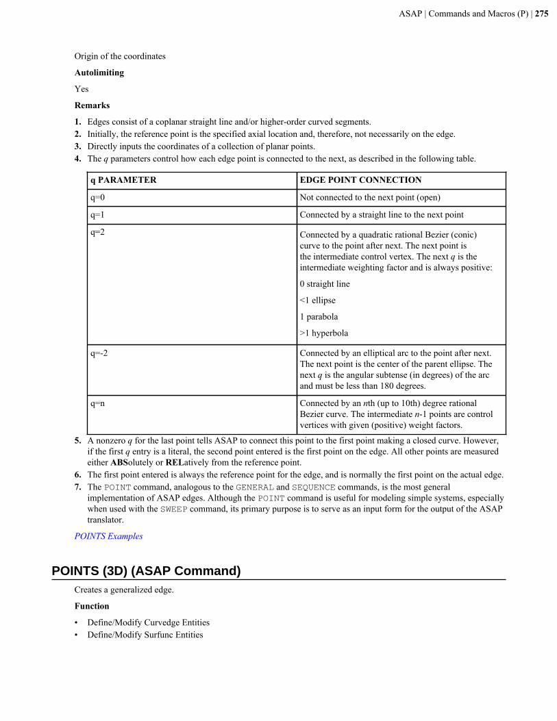
ASAP | Commands and Macros (P) | 275
Origin of the coordinates
Autolimiting
Yes
Remarks
1. Edges consist of a coplanar straight line and/or higher-order curved segments.2. Initially, the reference point is the specified axial location and, therefore, not necessarily on the edge.3. Directly inputs the coordinates of a collection of planar points.4. The q parameters control how each edge point is connected to the next, as described in the following table.
q PARAMETER EDGE POINT CONNECTION
q=0 Not connected to the next point (open)
q=1 Connected by a straight line to the next point
q=2 Connected by a quadratic rational Bezier (conic)curve to the point after next. The next point isthe intermediate control vertex. The next q is theintermediate weighting factor and is always positive:
0 straight line
<1 ellipse
1 parabola
>1 hyperbola
q=-2 Connected by an elliptical arc to the point after next.The next point is the center of the parent ellipse. Thenext q is the angular subtense (in degrees) of the arcand must be less than 180 degrees.
q=n Connected by an nth (up to 10th) degree rationalBezier curve. The intermediate n-1 points are controlvertices with given (positive) weight factors.
5. A nonzero q for the last point tells ASAP to connect this point to the first point making a closed curve. However,if the first q entry is a literal, the second point entered is the first point on the edge. All other points are measuredeither ABSolutely or RELatively from the reference point.
6. The first point entered is always the reference point for the edge, and is normally the first point on the actual edge.7. The POINT command, analogous to the GENERAL and SEQUENCE commands, is the most general
implementation of ASAP edges. Although the POINT command is useful for modeling simple systems, especiallywhen used with the SWEEP command, its primary purpose is to serve as an input form for the output of the ASAPtranslator.
POINTS Examples
POINTS (3D) (ASAP Command)Creates a generalized edge.
Function
• Define/Modify Curvedge Entities• Define/Modify Surfunc Entities
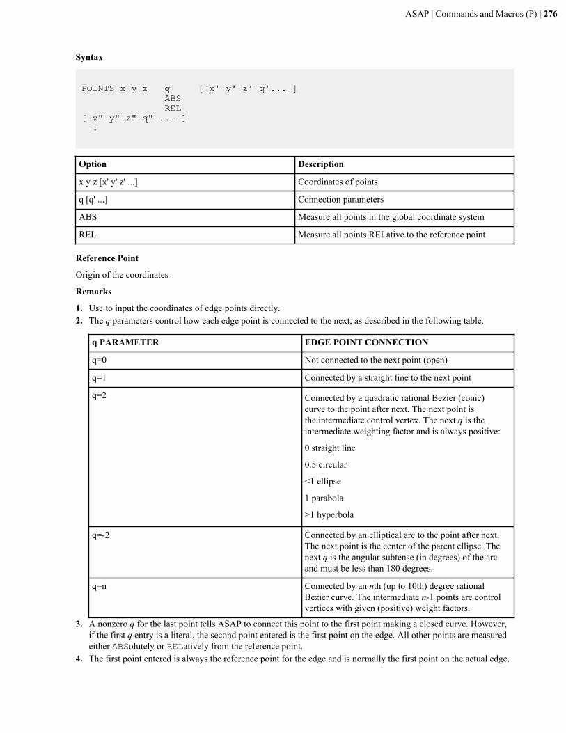
ASAP | Commands and Macros (P) | 276
Syntax
POINTS x y z q [ x' y' z' q'... ] ABS REL[ x" y" z" q" ... ] :
Option Description
x y z [x' y' z' ...] Coordinates of points
q [q' ...] Connection parameters
ABS Measure all points in the global coordinate system
REL Measure all points RELative to the reference point
Reference Point
Origin of the coordinates
Remarks
1. Use to input the coordinates of edge points directly.2. The q parameters control how each edge point is connected to the next, as described in the following table.
q PARAMETER EDGE POINT CONNECTION
q=0 Not connected to the next point (open)
q=1 Connected by a straight line to the next point
q=2 Connected by a quadratic rational Bezier (conic)curve to the point after next. The next point isthe intermediate control vertex. The next q is theintermediate weighting factor and is always positive:
0 straight line
0.5 circular
<1 ellipse
1 parabola
>1 hyperbola
q=-2 Connected by an elliptical arc to the point after next.The next point is the center of the parent ellipse. Thenext q is the angular subtense (in degrees) of the arcand must be less than 180 degrees.
q=n Connected by an nth (up to 10th) degree rationalBezier curve. The intermediate n-1 points are controlvertices with given (positive) weight factors.
3. A nonzero q for the last point tells ASAP to connect this point to the first point making a closed curve. However,if the first q entry is a literal, the second point entered is the first point on the edge. All other points are measuredeither ABSolutely or RELatively from the reference point.
4. The first point entered is always the reference point for the edge and is normally the first point on the actual edge.
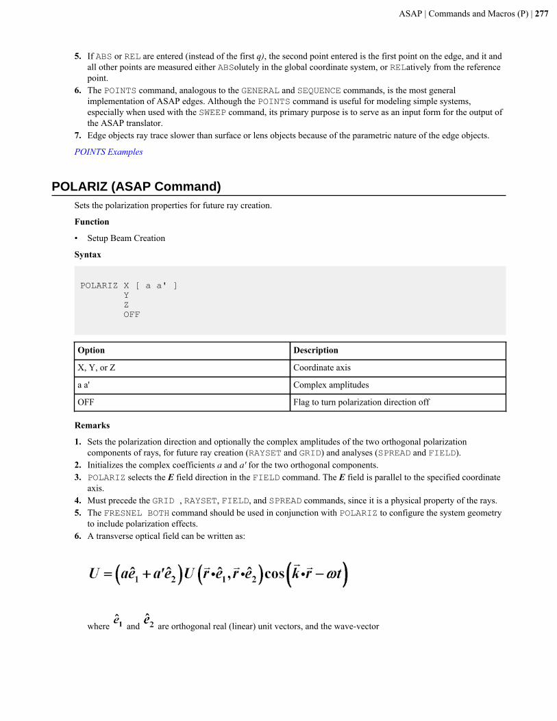
ASAP | Commands and Macros (P) | 277
5. If ABS or REL are entered (instead of the first q), the second point entered is the first point on the edge, and it andall other points are measured either ABSolutely in the global coordinate system, or RELatively from the referencepoint.
6. The POINTS command, analogous to the GENERAL and SEQUENCE commands, is the most generalimplementation of ASAP edges. Although the POINTS command is useful for modeling simple systems,especially when used with the SWEEP command, its primary purpose is to serve as an input form for the output ofthe ASAP translator.
7. Edge objects ray trace slower than surface or lens objects because of the parametric nature of the edge objects.
POINTS Examples
POLARIZ (ASAP Command)Sets the polarization properties for future ray creation.
Function
• Setup Beam Creation
Syntax
POLARIZ X [ a a' ] Y Z OFF
Option Description
X, Y, or Z Coordinate axis
a a' Complex amplitudes
OFF Flag to turn polarization direction off
Remarks
1. Sets the polarization direction and optionally the complex amplitudes of the two orthogonal polarizationcomponents of rays, for future ray creation (RAYSET and GRID) and analyses (SPREAD and FIELD).
2. Initializes the complex coefficients a and a' for the two orthogonal components.3. POLARIZ selects the E field direction in the FIELD command. The E field is parallel to the specified coordinate
axis.4. Must precede the GRID , RAYSET, FIELD, and SPREAD commands, since it is a physical property of the rays.5. The FRESNEL BOTH command should be used in conjunction with POLARIZ to configure the system geometry
to include polarization effects.6. A transverse optical field can be written as:
where and are orthogonal real (linear) unit vectors, and the wave-vector
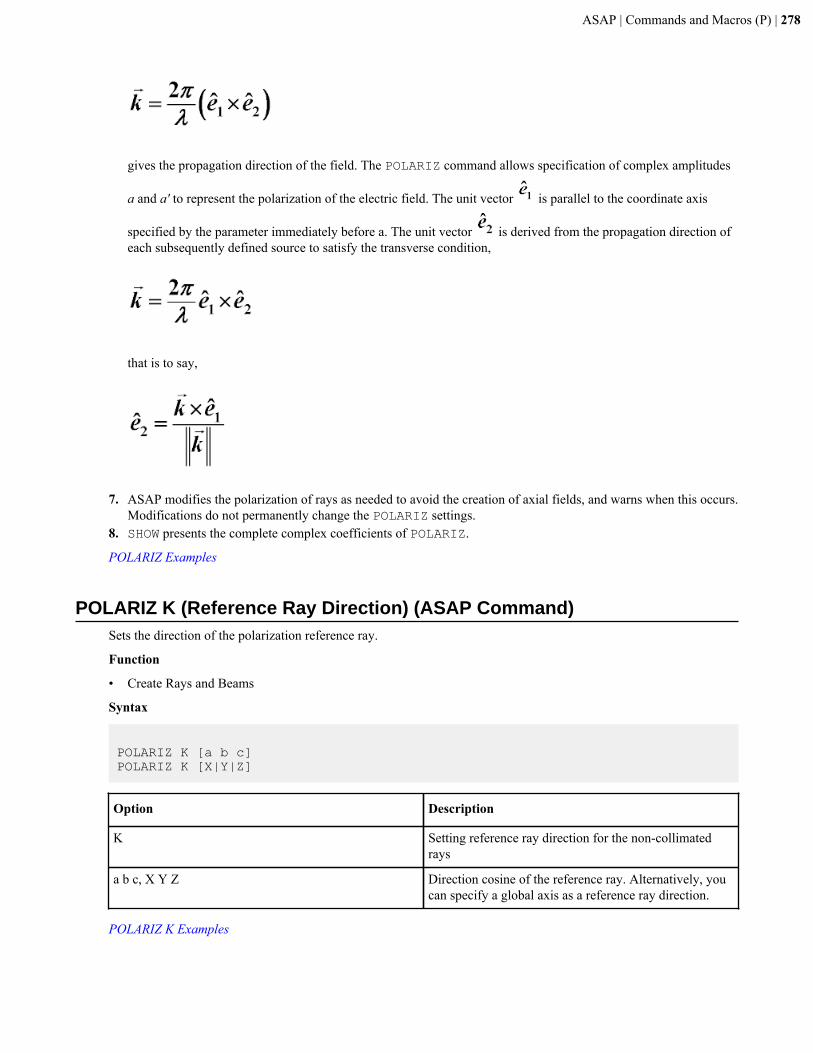
ASAP | Commands and Macros (P) | 278
gives the propagation direction of the field. The POLARIZ command allows specification of complex amplitudes
a and a' to represent the polarization of the electric field. The unit vector is parallel to the coordinate axis
specified by the parameter immediately before a. The unit vector is derived from the propagation direction ofeach subsequently defined source to satisfy the transverse condition,
that is to say,
7. ASAP modifies the polarization of rays as needed to avoid the creation of axial fields, and warns when this occurs.
Modifications do not permanently change the POLARIZ settings.8. SHOW presents the complete complex coefficients of POLARIZ.
POLARIZ Examples
POLARIZ K (Reference Ray Direction) (ASAP Command)Sets the direction of the polarization reference ray.
Function
• Create Rays and Beams
Syntax
POLARIZ K [a b c]POLARIZ K [X|Y|Z]
Option Description
K Setting reference ray direction for the non-collimatedrays
a b c, X Y Z Direction cosine of the reference ray. Alternatively, youcan specify a global axis as a reference ray direction.
POLARIZ K Examples
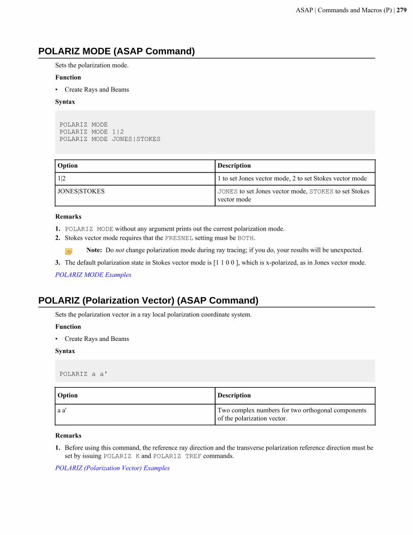
ASAP | Commands and Macros (P) | 279
POLARIZ MODE (ASAP Command)Sets the polarization mode.
Function
• Create Rays and Beams
Syntax
POLARIZ MODEPOLARIZ MODE 1|2POLARIZ MODE JONES|STOKES
Option Description
1|2 1 to set Jones vector mode, 2 to set Stokes vector mode
JONES|STOKES JONES to set Jones vector mode, STOKES to set Stokesvector mode
Remarks
1. POLARIZ MODE without any argument prints out the current polarization mode.2. Stokes vector mode requires that the FRESNEL setting must be BOTH.
Note: Do not change polarization mode during ray tracing; if you do, your results will be unexpected.
3. The default polarization state in Stokes vector mode is [1 1 0 0 ], which is x-polarized, as in Jones vector mode.
POLARIZ MODE Examples
POLARIZ (Polarization Vector) (ASAP Command)Sets the polarization vector in a ray local polarization coordinate system.
Function
• Create Rays and Beams
Syntax
POLARIZ a a'
Option Description
a a' Two complex numbers for two orthogonal componentsof the polarization vector.
Remarks
1. Before using this command, the reference ray direction and the transverse polarization reference direction must beset by issuing POLARIZ K and POLARIZ TREF commands.
POLARIZ (Polarization Vector) Examples
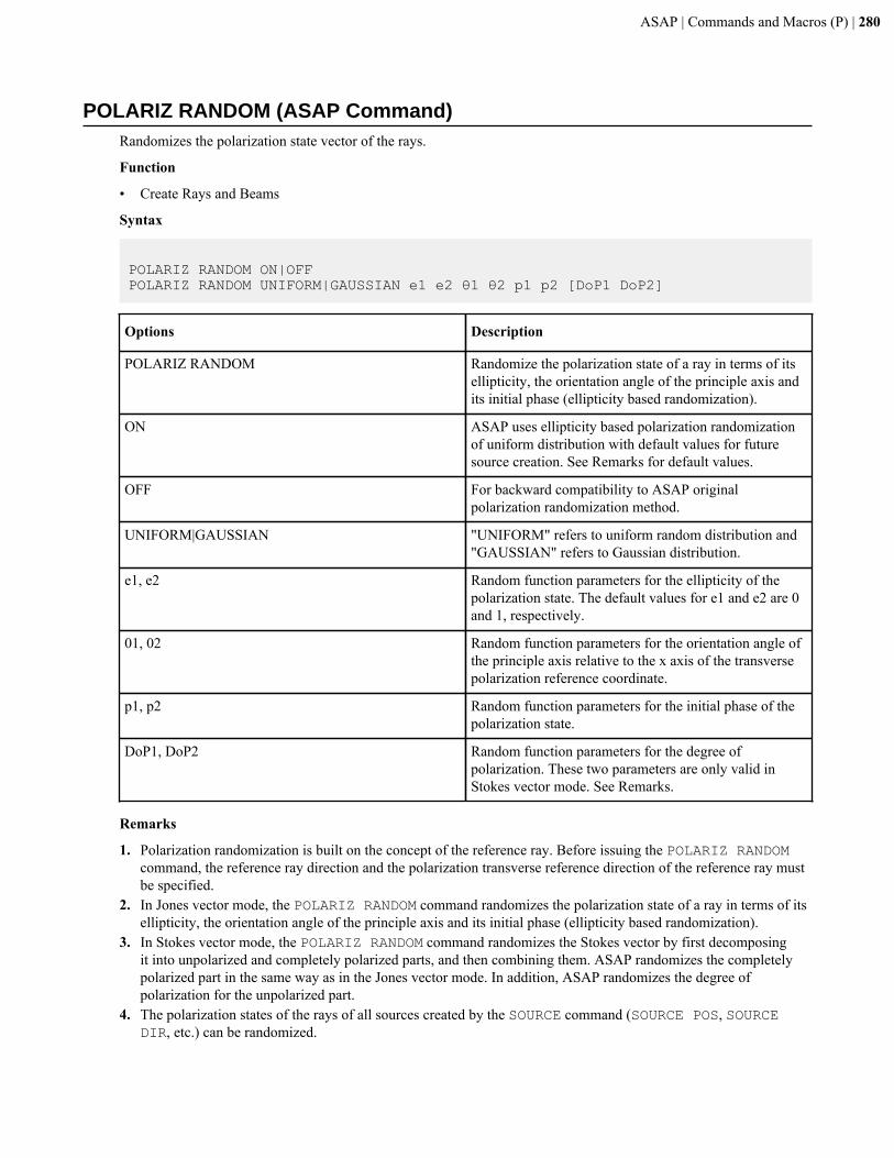
ASAP | Commands and Macros (P) | 280
POLARIZ RANDOM (ASAP Command)Randomizes the polarization state vector of the rays.
Function
• Create Rays and Beams
Syntax
POLARIZ RANDOM ON|OFFPOLARIZ RANDOM UNIFORM|GAUSSIAN e1 e2 θ1 θ2 p1 p2 [DoP1 DoP2]
Options Description
POLARIZ RANDOM Randomize the polarization state of a ray in terms of itsellipticity, the orientation angle of the principle axis andits initial phase (ellipticity based randomization).
ON ASAP uses ellipticity based polarization randomizationof uniform distribution with default values for futuresource creation. See Remarks for default values.
OFF For backward compatibility to ASAP originalpolarization randomization method.
UNIFORM|GAUSSIAN "UNIFORM" refers to uniform random distribution and"GAUSSIAN" refers to Gaussian distribution.
e1, e2 Random function parameters for the ellipticity of thepolarization state. The default values for e1 and e2 are 0and 1, respectively.
01, 02 Random function parameters for the orientation angle ofthe principle axis relative to the x axis of the transversepolarization reference coordinate.
p1, p2 Random function parameters for the initial phase of thepolarization state.
DoP1, DoP2 Random function parameters for the degree ofpolarization. These two parameters are only valid inStokes vector mode. See Remarks.
Remarks
1. Polarization randomization is built on the concept of the reference ray. Before issuing the POLARIZ RANDOMcommand, the reference ray direction and the polarization transverse reference direction of the reference ray mustbe specified.
2. In Jones vector mode, the POLARIZ RANDOM command randomizes the polarization state of a ray in terms of itsellipticity, the orientation angle of the principle axis and its initial phase (ellipticity based randomization).
3. In Stokes vector mode, the POLARIZ RANDOM command randomizes the Stokes vector by first decomposingit into unpolarized and completely polarized parts, and then combining them. ASAP randomizes the completelypolarized part in the same way as in the Jones vector mode. In addition, ASAP randomizes the degree ofpolarization for the unpolarized part.
4. The polarization states of the rays of all sources created by the SOURCE command (SOURCE POS, SOURCEDIR, etc.) can be randomized.
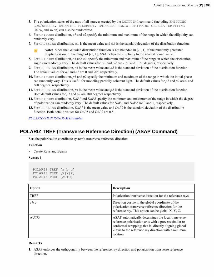
ASAP | Commands and Macros (P) | 281
5. The polarization states of the rays of all sources created by the EMITTING command (including EMITTINGBOX/SPHERE, EMITTING FILAMENT, EMITTING HELIX, EMITTING OBJECT, EMITTINGDATA, and so on) can also be randomized.
6. For UNIFORM distribution, e1 and e2 specify the minimum and maximum of the range in which the ellipticity canrandomly vary.
7. For GAUSSIAN distribution, e1 is the mean value and e2 is the standard deviation of the distribution function.
Note: Since the Gaussian distribution function is not bounded in [-1, 1], if the randomly generatedellipticity is out of the range of [-1, 1], ASAP clips the ellipticity to the nearest bound value.
8. For UNIFORM distribution, o1 and o2 specify the minimum and maximum of the range in which the orientationangle can randomly vary. The default values for o1 and o2 are -180 and +180 degrees, respectively.
9. For GAUSSIAN distribution, o1 is the mean value and o2 is the standard deviation of the distribution function.The default values for o1 and o2 are 0 and 90°, respectively.
10. For UNIFORM distribution, p1 and p2 specify the minimum and maximum of the range in which the initial phasecan randomly vary. This is useful for modeling partially coherent light. The default values for p1 and p2 are 0 and360 degrees, respectively.
11. For GAUSSIAN distribution, p1 is the mean value and p2 is the standard deviation of the distribution function.Both default values for p1 and p2 are 180 degrees respectively.
12. For UNIFORM distribution, DoP1 and DoP2 specify the minimum and maximum of the range in which the degreeof polarization can randomly vary. The default values for DoP1 and DoP2 are 0 and 1, respectively.
13. For GAUSSIAN distribution, DoP1 is the mean value and DoP2 is the standard deviation of the distributionfunction. Both default values for DoP1 and DoP2 are 0.5.
POLARIZATION RANDOM Examples
POLARIZ TREF (Transverse Reference Direction) (ASAP Command)Sets the polarization coordinate system's transverse reference direction.
Function
• Create Rays and Beams
Syntax 1
POLARIZ TREF [a b c] POLARIZ TREF [X|Y|Z] POLARIZ TREF [AUTO]
Option Description
TREF Polarization transverse direction for the reference rays.
a b c Direction cosine in the global coordinate of thepolarization transverse reference direction for thereference ray. This option can be global X, Y, Z.
AUTO ASAP automatically determines the local transversereference polarization axis with a process similar toconformal wrapping; that is, directly aligning globalZ axis to the reference ray direction with a minimumrotation.
Remarks
1. ASAP enforces the orthogonality between the reference ray direction and polarization transverse referencedirection.
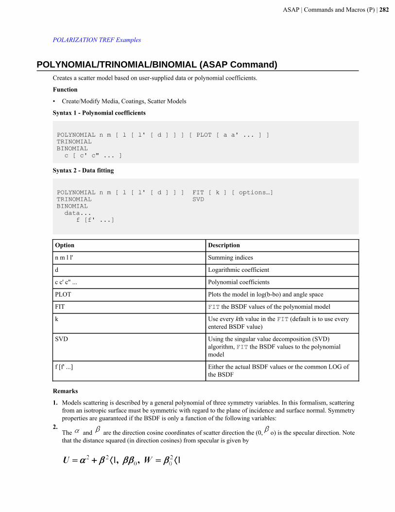
ASAP | Commands and Macros (P) | 282
POLARIZATION TREF Examples
POLYNOMIAL/TRINOMIAL/BINOMIAL (ASAP Command)Creates a scatter model based on user-supplied data or polynomial coefficients.
Function
• Create/Modify Media, Coatings, Scatter Models
Syntax 1 - Polynomial coefficients
POLYNOMIAL n m [ l [ l' [ d ] ] ] [ PLOT [ a a' ... ] ]TRINOMIALBINOMIAL c [ c' c" ... ]
Syntax 2 - Data fitting
POLYNOMIAL n m [ l [ l' [ d ] ] ] FIT [ k ] [ options…]TRINOMIAL SVDBINOMIAL data... f [f' ...]
Option Description
n m l l' Summing indices
d Logarithmic coefficient
c c' c" ... Polynomial coefficients
PLOT Plots the model in log(b-bo) and angle space
FIT FIT the BSDF values of the polynomial model
k Use every kth value in the FIT (default is to use everyentered BSDF value)
SVD Using the singular value decomposition (SVD)algorithm, FIT the BSDF values to the polynomialmodel
f [f' ...] Either the actual BSDF values or the common LOG ofthe BSDF
Remarks
1. Models scattering is described by a general polynomial of three symmetry variables. In this formalism, scatteringfrom an isotropic surface must be symmetric with regard to the plane of incidence and surface normal. Symmetryproperties are guaranteed if the BSDF is only a function of the following variables:
2.The and are the direction cosine coordinates of scatter direction the (0, o) is the specular direction. Notethat the distance squared (in direction cosines) from specular is given by

ASAP | Commands and Macros (P) | 283
3. The scattering is modeled by a general polynomial of 2 or 3 symmetry variables with coefficients c ... (up to 286);
that is:
POLYNOMIAL
TRINOMIAL
BINOMIAL
4. If m is entered as a negative number, the upper limit of the second sum becomes |m|-k. The coefficients are
entered in the order in which they appear in the previous equations for the given n m l l'.5. Note that if d is zero, all the Lorentzian (log specular) terms vanish.6. If FIT or SVD is entered, ASAP fits the user-supplied BSDF data to the specified polynomial form. Under the SVD
option, a limited number of data points can be fitted. (See DIMENSIONS command output.)7. By default, every BSDF value entered (above 1.E-9, -9 LOG) is used in the fit. Optionally, only every kth value
can be used.8. The restricted variables used in the BINOMIAL form and the term symmetry in the POLYNOMIAL form assure
that the resulting BSDF exactly obeys reciprocity. The TRINOMIAL form is not, by definition, reciprocal; but,
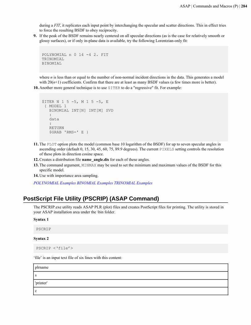
ASAP | Commands and Macros (P) | 284
during a FIT, it replicates each input point by interchanging the specular and scatter directions. This in effect triesto force the resulting BSDF to obey reciprocity.
9. If the peak of the BSDF remains nearly centered on all specular directions (as is the case for relatively smooth orglossy surfaces), or if only in-plane data is available, try the following Lorentzian-only fit:
POLYNOMIAL n 0 14 -4 2. FITTRINOMIALBINOMIAL
where n is less than or equal to the number of non-normal incident directions in the data. This generates a modelwith 20(n+1) coefficients. Confirm that there are at least as many BSDF values (a few times more is better).
10. Another more general technique is to use $ITER to do a "regressive" fit. For example:
$ITER N 1 5 -5, M 1 5 -5, E { MODEL 1 BINOMIAL INT[N] INT[M] SVD : data : RETURN $GRAB 'RMS=' E }
11. The PLOT option plots the model (common base 10 logarithm of the BSDF) for up to seven specular angles inascending order (default 0, 15, 30, 45, 60, 75, 89.9 degrees). The current PIXELS setting controls the resolutionof these plots in direction cosine space.
12. Creates a distribution file name_angle.dis for each of these angles.13. The command argument, MINMAX may be used to set the minimum and maximum values of the BSDF for this
specific model.14. Use with importance area sampling.
POLYNOMIAL Examples BINOMIAL Examples TRINOMIAL Examples
PostScript File Utility (PSCRIP) (ASAP Command)The PSCRIP.exe utility reads ASAP PLR (plot) files and creates PostScript files for printing. The utility is stored inyour ASAP installation area under the \bin folder.
Syntax 1
PSCRIP
Syntax 2
PSCRIP <‘file’>
‘file’ is an input text file of six lines with this content:
plrname
s
'printer'
c
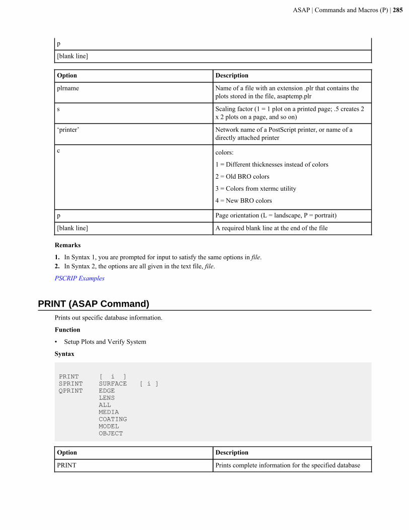
ASAP | Commands and Macros (P) | 285
p
[blank line]
Option Description
plrname Name of a file with an extension .plr that contains theplots stored in the file, asaptemp.plr
s Scaling factor (1 = 1 plot on a printed page; .5 creates 2x 2 plots on a page, and so on)
‘printer’ Network name of a PostScript printer, or name of adirectly attached printer
c colors:
1 = Different thicknesses instead of colors
2 = Old BRO colors
3 = Colors from xtermc utility
4 = New BRO colors
p Page orientation (L = landscape, P = portrait)
[blank line] A required blank line at the end of the file
Remarks
1. In Syntax 1, you are prompted for input to satisfy the same options in file.2. In Syntax 2, the options are all given in the text file, file.
PSCRIP Examples
PRINT (ASAP Command)Prints out specific database information.
Function
• Setup Plots and Verify System
Syntax
PRINT [ i ]SPRINT SURFACE [ i ]QPRINT EDGE LENS ALL MEDIA COATING MODEL OBJECT
Option Description
PRINT Prints complete information for the specified database
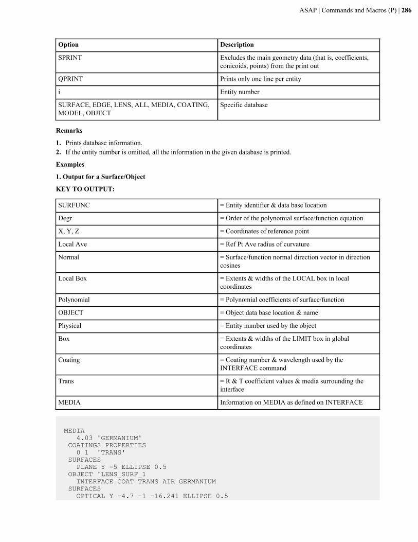
ASAP | Commands and Macros (P) | 286
Option Description
SPRINT Excludes the main geometry data (that is, coefficients,conicoids, points) from the print out
QPRINT Prints only one line per entity
i Entity number
SURFACE, EDGE, LENS, ALL, MEDIA, COATING,MODEL, OBJECT
Specific database
Remarks
1. Prints database information.2. If the entity number is omitted, all the information in the given database is printed.
Examples
1. Output for a Surface/Object
KEY TO OUTPUT:
SURFUNC = Entity identifier & data base location
Degr = Order of the polynomial surface/function equation
X, Y, Z = Coordinates of reference point
Local Ave = Ref Pt Ave radius of curvature
Normal = Surface/function normal direction vector in directioncosines
Local Box = Extents & widths of the LOCAL box in localcoordinates
Polynomial = Polynomial coefficients of surface/function
OBJECT = Object data base location & name
Physical = Entity number used by the object
Box = Extents & widths of the LIMIT box in globalcoordinates
Coating = Coating number & wavelength used by theINTERFACE command
Trans = R & T coefficient values & media surrounding theinterface
MEDIA Information on MEDIA as defined on INTERFACE
MEDIA 4.03 'GERMANIUM' COATINGS PROPERTIES 0 1 'TRANS' SURFACES PLANE Y -5 ELLIPSE 0.5 OBJECT 'LENS_SURF_1 INTERFACE COAT TRANS AIR GERMANIUM SURFACES OPTICAL Y -4.7 -1 -16.241 ELLIPSE 0.5
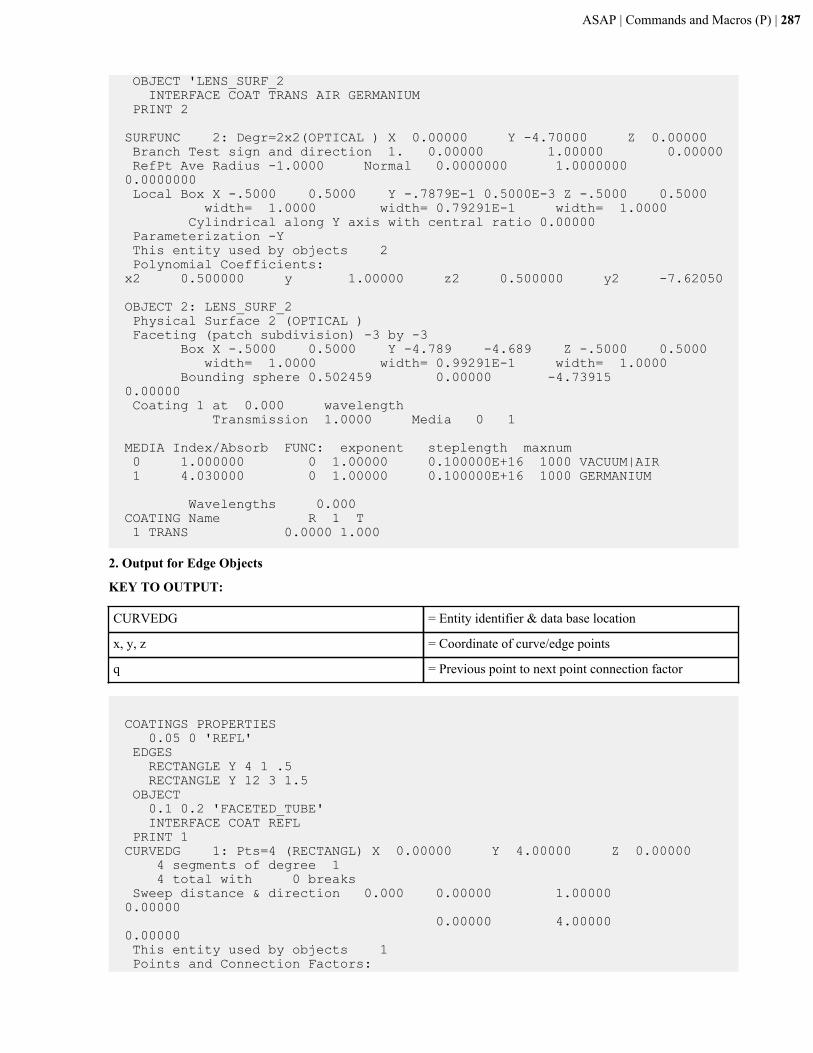
ASAP | Commands and Macros (P) | 287
OBJECT 'LENS_SURF_2 INTERFACE COAT TRANS AIR GERMANIUM PRINT 2 SURFUNC 2: Degr=2x2(OPTICAL ) X 0.00000 Y -4.70000 Z 0.00000 Branch Test sign and direction 1. 0.00000 1.00000 0.00000 RefPt Ave Radius -1.0000 Normal 0.0000000 1.0000000 0.0000000 Local Box X -.5000 0.5000 Y -.7879E-1 0.5000E-3 Z -.5000 0.5000 width= 1.0000 width= 0.79291E-1 width= 1.0000 Cylindrical along Y axis with central ratio 0.00000 Parameterization -Y This entity used by objects 2 Polynomial Coefficients: x2 0.500000 y 1.00000 z2 0.500000 y2 -7.62050
OBJECT 2: LENS_SURF_2 Physical Surface 2 (OPTICAL ) Faceting (patch subdivision) -3 by -3 Box X -.5000 0.5000 Y -4.789 -4.689 Z -.5000 0.5000 width= 1.0000 width= 0.99291E-1 width= 1.0000 Bounding sphere 0.502459 0.00000 -4.73915 0.00000 Coating 1 at 0.000 wavelength Transmission 1.0000 Media 0 1
MEDIA Index/Absorb FUNC: exponent steplength maxnum 0 1.000000 0 1.00000 0.100000E+16 1000 VACUUM|AIR 1 4.030000 0 1.00000 0.100000E+16 1000 GERMANIUM
Wavelengths 0.000 COATING Name R 1 T 1 TRANS 0.0000 1.000
2. Output for Edge Objects
KEY TO OUTPUT:
CURVEDG = Entity identifier & data base location
x, y, z = Coordinate of curve/edge points
q = Previous point to next point connection factor
COATINGS PROPERTIES 0.05 0 'REFL' EDGES RECTANGLE Y 4 1 .5 RECTANGLE Y 12 3 1.5 OBJECT 0.1 0.2 'FACETED_TUBE' INTERFACE COAT REFL PRINT 1 CURVEDG 1: Pts=4 (RECTANGL) X 0.00000 Y 4.00000 Z 0.00000 4 segments of degree 1 4 total with 0 breaks Sweep distance & direction 0.000 0.00000 1.00000 0.00000 0.00000 4.00000 0.00000 This entity used by objects 1 Points and Connection Factors:

ASAP | Commands and Macros (P) | 288
x y z q x y z q -0.500000 0.000000 1.000000 1.00000 0.500000 0.000000 1.000000 1.00000 0.500000 0.000000 -1.000000 1.00000 -0.500000 0.000000 -1.000000 1.00000
CURVEDG 2: Pts=4 (RECTANGL) X 0.00000 Y 12.0000 Z 0.00000 4 segments of degree 1 4 total with 0 breaks Sweep distance & direction 0.000 0.00000 1.00000 0.00000 0.00000 12.0000 0.00000 This entity used by objects 1 Points and Connection Factors: x y z q x y z q -1.500000 0.000000 3.000000 1.00000 1.500000 0.000000 3.000000 1.00000 1.500000 0.000000 -3.000000 1.00000 -1.500000 0.000000 -3.000000 1.00000
OBJECT 1: FACETED_TUBE Physical Surface 2 (RECTANGL) to 1 (RECTANGL) 1 segments of degree 1 1 total with 1 breaks Faceting (patch subdivision) +1 by +1 Box X -1.580 1.580 Y 3.920 12.08 Z -3.080 3.080 width= 3.1600 width= 8.1600 width= 6.1600 Bounding sphere 5.35063 0.596046E-07 8.00000 0.00000 Coating 1 at 0.000 wavelength Interface Reflectivity 0.50000E-01
Wavelengths 0.000 COATING Name R 1 T
3. Output for Lens Objects
KEY TO OUTPUT:
LENS = Entity identifier & data base location
Srfs = Number of conicoids of lens
X, Y, Z = Coordinates of reference point
Conicoid Data:
X, Y, Z = Coordinates of first conicoid
A, B, C = Conicoid normal direction vector in direction cosines
APT = Conicoid aperture semi-diameter
CRV = Conicoid base curvature
CON = Conicoid conic constant
OBS = Conicoid obscuration ratio
MED = Media after conicoid
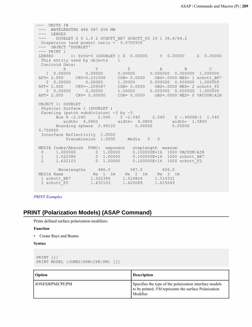
ASAP | Commands and Macros (P) | 289
--- UNITS IN --- WAVELENGTHS 486 587 656 NM --- LENSES --- DOUBLET Z 0 1.5 2 SCHOTT_BK7 SCHOTT_F2 10 1 36.6/64.2 Dispersion (and power) ratio = 0.5700935 --- OBJECT 'DOUBLET' --- PRINT 1 LENSES 1: Srfs=3 (DOUBLET ) X 0.00000 Y 0.00000 Z 0.00000 This entity used by objects 1 Conicoid Data: X Y Z A B C 1 0.00000 0.00000 0.00000 0.000000 0.000000 1.000000 APT= 2.000 CRV=0.231506 CON= 0.0000 OBS=.0000 MED= 1 schott_BK7 2 0.00000 0.00000 1.35000 0.000000 0.000000 1.000000 APT= 2.000 CRV=-.209587 CON= 0.0000 OBS=.0000 MED= 2 schott_F2 3 0.00000 0.00000 1.50000 0.000000 0.000000 1.000000 APT= 2.000 CRV= 0.00000 CON= 0.0000 OBS=.0000 MED= 0 VACUUM|AIR
OBJECT 1: DOUBLET Physical Surface 1 (DOUBLET ) Faceting (patch subdivision) -3 by -3 Box X -2.040 2.040 Y -2.040 2.040 Z -.4000E-1 1.540 width= 4.0800 width= 4.0800 width= 1.5800 Bounding sphere 2.99120 0.00000 0.00000 0.750000 Interface Reflectivity 1.0000 Transmission 1.0000 Media 0 0
MEDIA Index/Absorb FUNC: exponent steplength maxnum 0 1.000000 0 1.00000 0.100000E+16 1000 VACUUM|AIR 1 1.522386 0 1.00000 0.100000E+16 1000 schott_BK7 2 1.632103 0 1.00000 0.100000E+16 1000 schott_F2
Wavelengths 486.0 587.0 656.0 MEDIA Name Re 1 Im Re 2 Im Re 3 Im 1 schott_BK7 1.522386 1.516824 1.514331 2 schott_F2 1.632103 1.620089 1.615049
PRINT Examples
PRINT (Polarization Models) (ASAP Command)Prints defined surface polarization modifiers.
Function
• Create Rays and Beams
Syntax
PRINT [i] PRINT MODEL {JONES|RPM|CPE|PM} [j]
Option Description
JONES|RPM|CPE|PM Specifies the type of the polarization interface modelsto be printed. PM represents the surface PolarizationModifier.
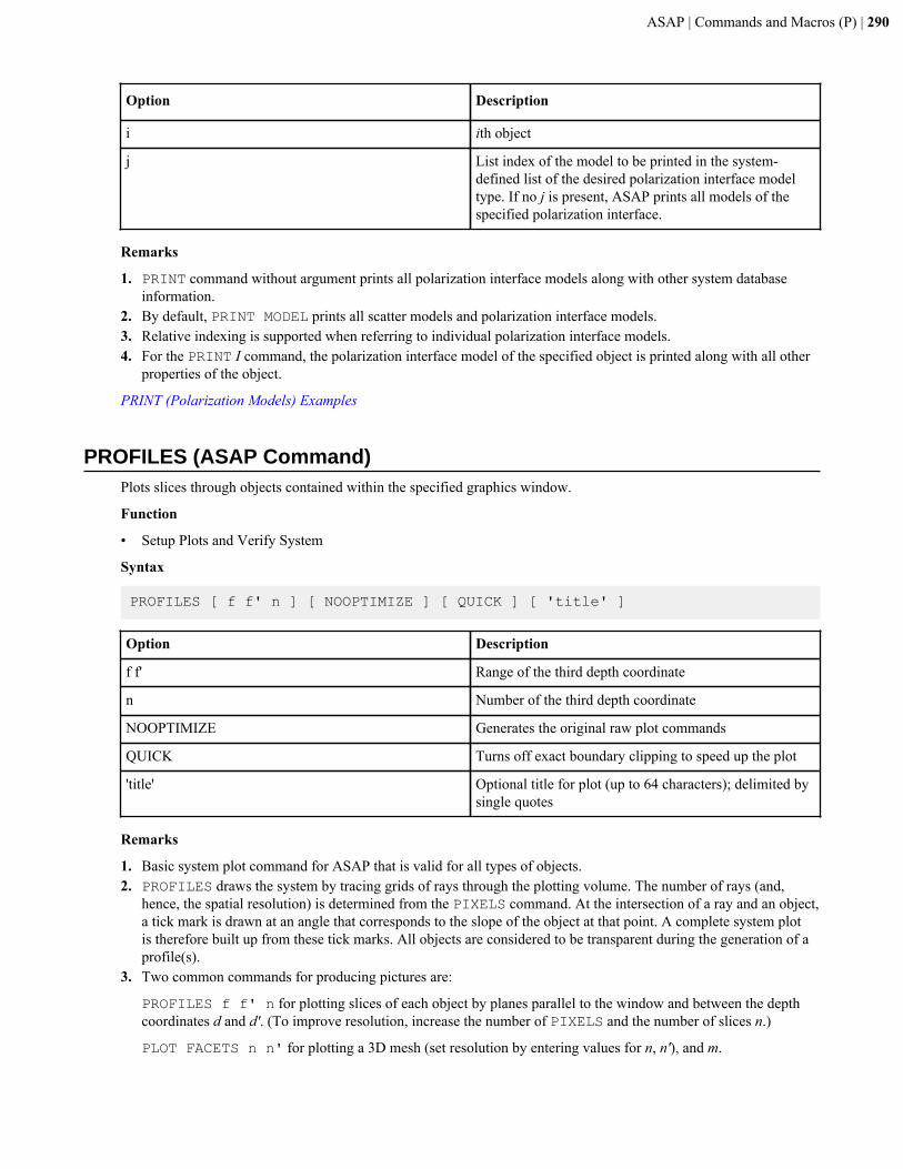
ASAP | Commands and Macros (P) | 290
Option Description
i ith object
j List index of the model to be printed in the system-defined list of the desired polarization interface modeltype. If no j is present, ASAP prints all models of thespecified polarization interface.
Remarks
1. PRINT command without argument prints all polarization interface models along with other system databaseinformation.
2. By default, PRINT MODEL prints all scatter models and polarization interface models.3. Relative indexing is supported when referring to individual polarization interface models.4. For the PRINT I command, the polarization interface model of the specified object is printed along with all other
properties of the object.
PRINT (Polarization Models) Examples
PROFILES (ASAP Command)Plots slices through objects contained within the specified graphics window.
Function
• Setup Plots and Verify System
Syntax
PROFILES [ f f' n ] [ NOOPTIMIZE ] [ QUICK ] [ 'title' ]
Option Description
f f' Range of the third depth coordinate
n Number of the third depth coordinate
NOOPTIMIZE Generates the original raw plot commands
QUICK Turns off exact boundary clipping to speed up the plot
'title' Optional title for plot (up to 64 characters); delimited bysingle quotes
Remarks
1. Basic system plot command for ASAP that is valid for all types of objects.2. PROFILES draws the system by tracing grids of rays through the plotting volume. The number of rays (and,
hence, the spatial resolution) is determined from the PIXELS command. At the intersection of a ray and an object,a tick mark is drawn at an angle that corresponds to the slope of the object at that point. A complete system plotis therefore built up from these tick marks. All objects are considered to be transparent during the generation of aprofile(s).
3. Two common commands for producing pictures are:
PROFILES f f' n for plotting slices of each object by planes parallel to the window and between the depthcoordinates d and d'. (To improve resolution, increase the number of PIXELS and the number of slices n.)
PLOT FACETS n n' for plotting a 3D mesh (set resolution by entering values for n, n'), and m.
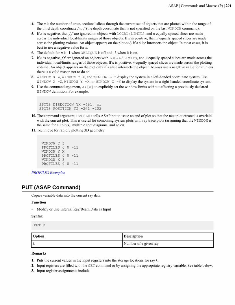
ASAP | Commands and Macros (P) | 291
4. The n is the number of cross-sectional slices through the current set of objects that are plotted within the range ofthe third depth coordinate f to f' (the depth coordinate that is not specified on the last WINDOW command).
5. If n is negative, then f f' are ignored on objects with LOCAL/LIMITS, and n equally spaced slices are madeacross the individual local/limits ranges of those objects. If n is positive, then n equally spaced slices are madeacross the plotting volume. An object appears on the plot only if a slice intersects the object. In most cases, it isbest to use a negative value for n.
6. The default for n is -1 when OBLIQUE is off and -5 when it is on.7. If n is negative, f f' are ignored on objects with LOCAL/LIMITS, and n equally spaced slices are made across the
individual local/limits ranges of those objects. If n is positive, n equally spaced slices are made across the plottingvolume. An object appears on the plot only if a slice intersects the object. Always use a negative value for n unlessthere is a valid reason not to do so.
8. WINDOW X Z, WINDOW Y X, and WINDOW Z Y display the system in a left-handed coordinate system. UseWINDOW X -Z, WINDOW Y -X, or WINDOW Z -Y to display the system in a right-handed coordinate system.
9. Use the command argument, XY[Z] to explicitly set the window limits without affecting a previously declaredWINDOW definition. For example:
SPOTS DIRECTION YX -4@1, orSPOTS POSITION YZ -2@1 -2@2
10. The command argument, OVERLAY tells ASAP not to issue an end of plot so that the next plot created is overlaidwith the current plot. This is useful for combining system plots with ray trace plots (assuming that the WINDOW isthe same for all plots), multiple spot diagrams, and so on.
11. Technique for rapidly plotting 3D geometry:
WINDOW Y Z PROFILES 0 0 -11 WINDOW Y X PROFILES 0 0 -11 WINDOW X Z PROFILES 0 0 -11
PROFILES Examples
PUT (ASAP Command)Copies variable data into the current ray data.
Function
• Modify or Use Internal Ray/Beam Data as Input
Syntax
PUT k
Option Description
k Number of a given ray
Remarks
1. Puts the current values in the input registers into the storage locations for ray k.2. Input registers are filled with the GET command or by assigning the appropriate registry variable. See table below.3. Input register assignments include:
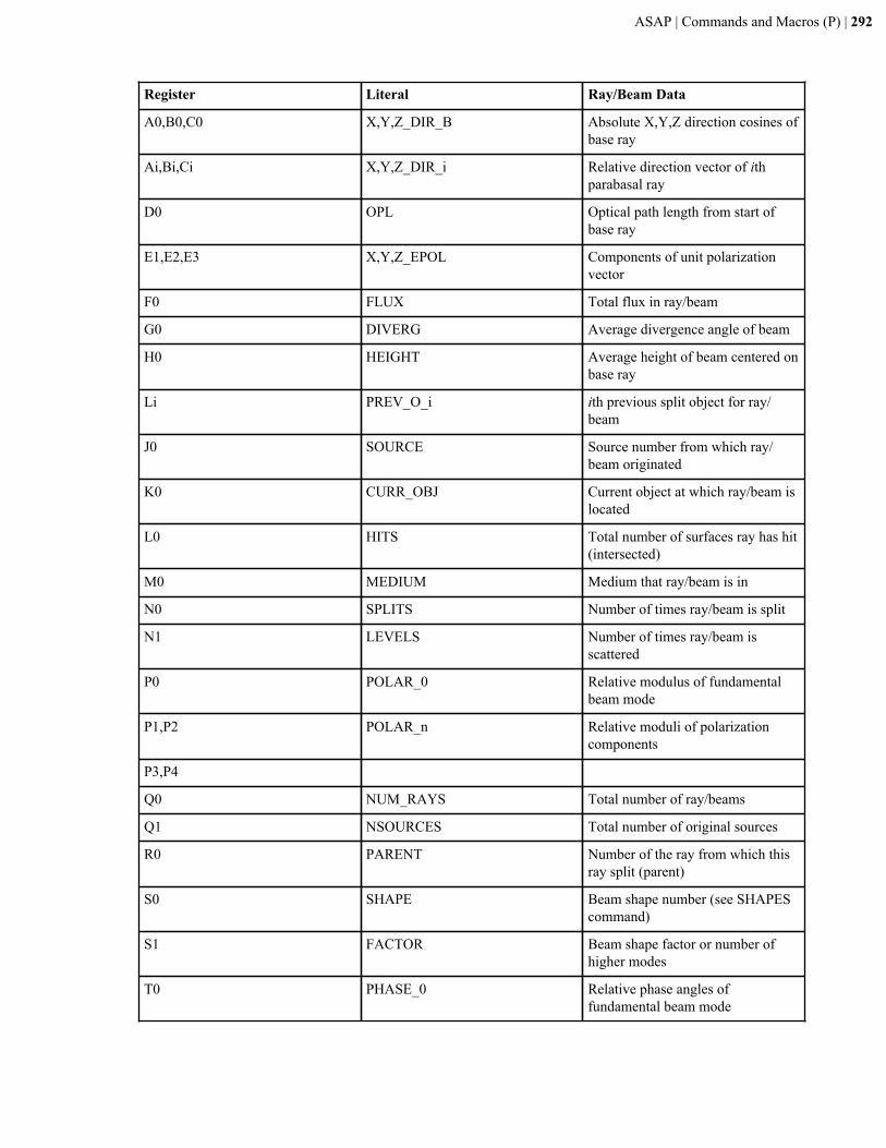
ASAP | Commands and Macros (P) | 292
Register Literal Ray/Beam Data
A0,B0,C0 X,Y,Z_DIR_B Absolute X,Y,Z direction cosines ofbase ray
Ai,Bi,Ci X,Y,Z_DIR_i Relative direction vector of ithparabasal ray
D0 OPL Optical path length from start ofbase ray
E1,E2,E3 X,Y,Z_EPOL Components of unit polarizationvector
F0 FLUX Total flux in ray/beam
G0 DIVERG Average divergence angle of beam
H0 HEIGHT Average height of beam centered onbase ray
Li PREV_O_i ith previous split object for ray/beam
J0 SOURCE Source number from which ray/beam originated
K0 CURR_OBJ Current object at which ray/beam islocated
L0 HITS Total number of surfaces ray has hit(intersected)
M0 MEDIUM Medium that ray/beam is in
N0 SPLITS Number of times ray/beam is split
N1 LEVELS Number of times ray/beam isscattered
P0 POLAR_0 Relative modulus of fundamentalbeam mode
P1,P2 POLAR_n Relative moduli of polarizationcomponents
P3,P4
Q0 NUM_RAYS Total number of ray/beams
Q1 NSOURCES Total number of original sources
R0 PARENT Number of the ray from which thisray split (parent)
S0 SHAPE Beam shape number (see SHAPEScommand)
S1 FACTOR Beam shape factor or number ofhigher modes
T0 PHASE_0 Relative phase angles offundamental beam mode
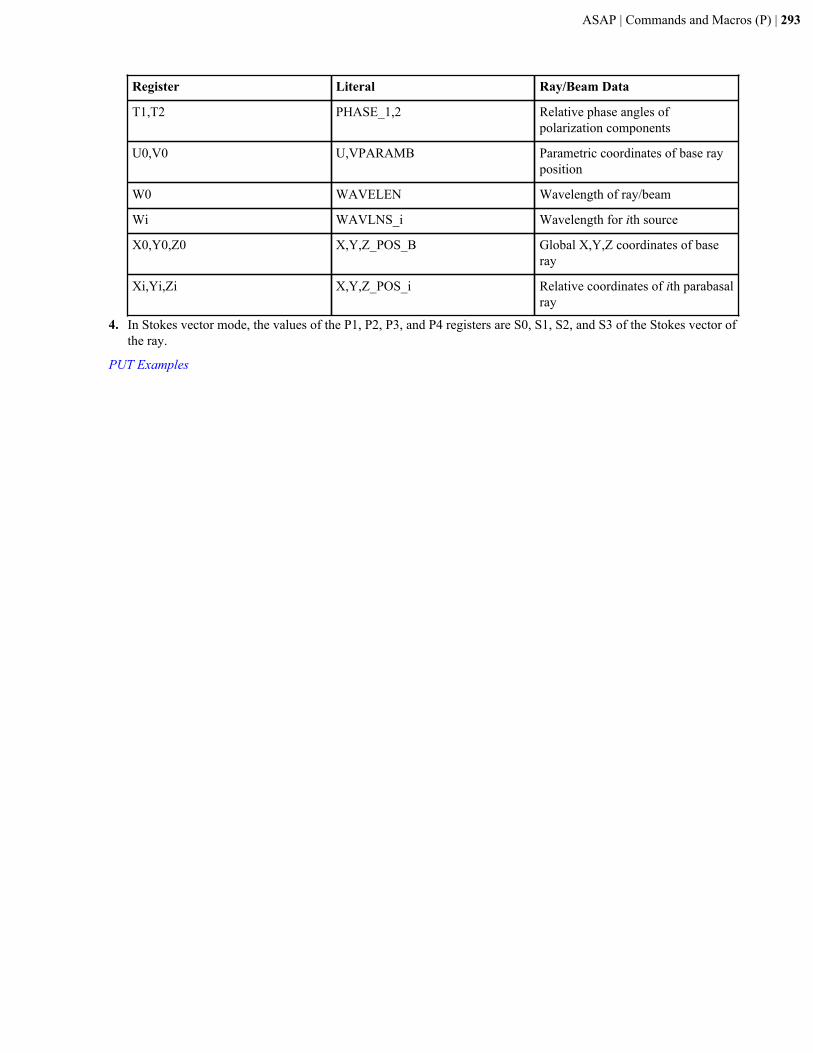
ASAP | Commands and Macros (P) | 293
Register Literal Ray/Beam Data
T1,T2 PHASE_1,2 Relative phase angles ofpolarization components
U0,V0 U,VPARAMB Parametric coordinates of base rayposition
W0 WAVELEN Wavelength of ray/beam
Wi WAVLNS_i Wavelength for ith source
X0,Y0,Z0 X,Y,Z_POS_B Global X,Y,Z coordinates of baseray
Xi,Yi,Zi X,Y,Z_POS_i Relative coordinates of ith parabasalray
4. In Stokes vector mode, the values of the P1, P2, P3, and P4 registers are S0, S1, S2, and S3 of the Stokes vector ofthe ray.
PUT Examples
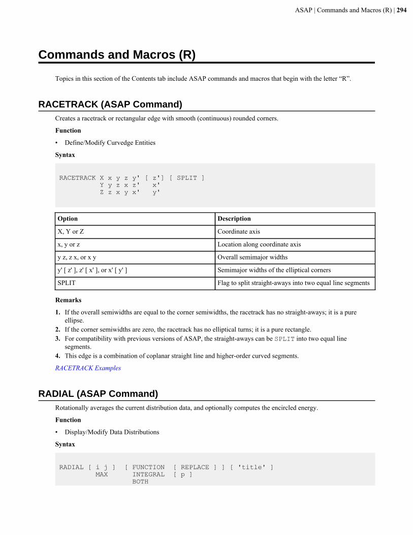
ASAP | Commands and Macros (R) | 294
Commands and Macros (R)
Topics in this section of the Contents tab include ASAP commands and macros that begin with the letter “R”.
RACETRACK (ASAP Command)Creates a racetrack or rectangular edge with smooth (continuous) rounded corners.
Function
• Define/Modify Curvedge Entities
Syntax
RACETRACK X x y z y' [ z'] [ SPLIT ] Y y z x z' x' Z z x y x' y'
Option Description
X, Y or Z Coordinate axis
x, y or z Location along coordinate axis
y z, z x, or x y Overall semimajor widths
y' [ z' ], z' [ x' ], or x' [ y' ] Semimajor widths of the elliptical corners
SPLIT Flag to split straight-aways into two equal line segments
Remarks
1. If the overall semiwidths are equal to the corner semiwidths, the racetrack has no straight-aways; it is a pureellipse.
2. If the corner semiwidths are zero, the racetrack has no elliptical turns; it is a pure rectangle.3. For compatibility with previous versions of ASAP, the straight-aways can be SPLIT into two equal line
segments.4. This edge is a combination of coplanar straight line and higher-order curved segments.
RACETRACK Examples
RADIAL (ASAP Command)Rotationally averages the current distribution data, and optionally computes the encircled energy.
Function
• Display/Modify Data Distributions
Syntax
RADIAL [ i j ] [ FUNCTION [ REPLACE ] ] [ 'title' ] MAX INTEGRAL [ p ] BOTH
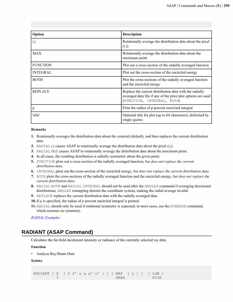
ASAP | Commands and Macros (R) | 295
Option Description
i j Rotationally average the distribution data about the pixel(i j)
MAX Rotationally average the distribution data about themaximum point
FUNCTION Plot out a cross-section of the radially averaged function
INTEGRAL Plot out the cross-section of the encircled energy
BOTH Plot the cross-sections of the radially averaged functionand the encircled energy
REPLACE Replace the current distribution data with the radiallyaveraged data file if any of the prior plot options are used(FUNCTION, INTEGRAL, BOTH)
p Print the radius of p percent encircled integral
'title' Optional title for plot (up to 64 characters); delimited bysingle quotes
Remarks
1. Rotationally averages the distribution data about the centroid (default), and then replaces the current distributiondata.
2. RADIAL i j causes ASAP to rotationally average the distribution data about the pixel (i j).3. RADIAL MAX causes ASAP to rotationally average the distribution data about the maximum point.4. In all cases, the resulting distribution is radially symmetric about the given point.5. FUNCTION plots out a cross-section of the radially averaged function, but does not replace the current
distribution data.6. INTEGRAL plots out the cross-section of the encircled energy, but does not replace the current distribution data.7. BOTH plots the cross-sections of the radially averaged function and the encircled energy, but does not replace the
current distribution data.8. RADIAL BOTH and RADIAL INTEGRAL should not be used after the ANGLES command if averaging directional
distributions. ANGLES remapping distorts the coordinate system, making the radial average invalid.9. REPLACE replaces the current distribution data with the radially averaged data.10. If p is specified, the radius of p percent encircled integral is printed.11.RADIAL should only be used if rotational symmetry is expected; in most cases, use the AVERAGE command,
which assumes no symmetry.
RADIAL Examples
RADIANT (ASAP Command)Calculates the far-field incoherent intensity or radiance of the currently selected ray data.
Function
• Analyze Ray/Beam Data
Syntax
RADIANT [ X [ f f' n a a' n' ] ] [ MAP [ s ] ] [ LOW ] Y AREA HIGH
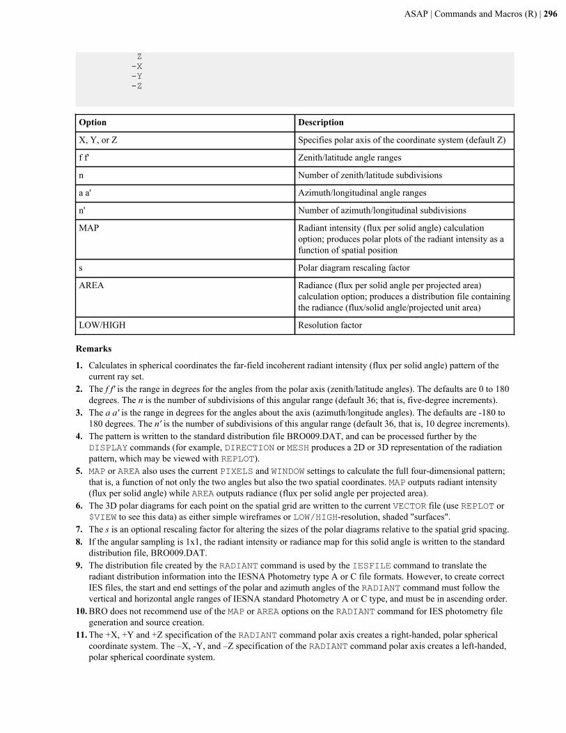
ASAP | Commands and Macros (R) | 296
Z -X -Y -Z
Option Description
X, Y, or Z Specifies polar axis of the coordinate system (default Z)
f f' Zenith/latitude angle ranges
n Number of zenith/latitude subdivisions
a a' Azimuth/longitudinal angle ranges
n' Number of azimuth/longitudinal subdivisions
MAP Radiant intensity (flux per solid angle) calculationoption; produces polar plots of the radiant intensity as afunction of spatial position
s Polar diagram rescaling factor
AREA Radiance (flux per solid angle per projected area)calculation option; produces a distribution file containingthe radiance (flux/solid angle/projected unit area)
LOW/HIGH Resolution factor
Remarks
1. Calculates in spherical coordinates the far-field incoherent radiant intensity (flux per solid angle) pattern of thecurrent ray set.
2. The f f' is the range in degrees for the angles from the polar axis (zenith/latitude angles). The defaults are 0 to 180degrees. The n is the number of subdivisions of this angular range (default 36; that is, five-degree increments).
3. The a a' is the range in degrees for the angles about the axis (azimuth/longitude angles). The defaults are -180 to180 degrees. The n' is the number of subdivisions of this angular range (default 36, that is, 10 degree increments).
4. The pattern is written to the standard distribution file BRO009.DAT, and can be processed further by theDISPLAY commands (for example, DIRECTION or MESH produces a 2D or 3D representation of the radiationpattern, which may be viewed with REPLOT).
5. MAP or AREA also uses the current PIXELS and WINDOW settings to calculate the full four-dimensional pattern;that is, a function of not only the two angles but also the two spatial coordinates. MAP outputs radiant intensity(flux per solid angle) while AREA outputs radiance (flux per solid angle per projected area).
6. The 3D polar diagrams for each point on the spatial grid are written to the current VECTOR file (use REPLOT or$VIEW to see this data) as either simple wireframes or LOW/HIGH-resolution, shaded "surfaces".
7. The s is an optional rescaling factor for altering the sizes of the polar diagrams relative to the spatial grid spacing.8. If the angular sampling is 1x1, the radiant intensity or radiance map for this solid angle is written to the standard
distribution file, BRO009.DAT.9. The distribution file created by the RADIANT command is used by the IESFILE command to translate the
radiant distribution information into the IESNA Photometry type A or C file formats. However, to create correctIES files, the start and end settings of the polar and azimuth angles of the RADIANT command must follow thevertical and horizontal angle ranges of IESNA standard Photometry A or C type, and must be in ascending order.
10. BRO does not recommend use of the MAP or AREA options on the RADIANT command for IES photometry filegeneration and source creation.
11. The +X, +Y and +Z specification of the RADIANT command polar axis creates a right-handed, polar sphericalcoordinate system. The –X, -Y, and –Z specification of the RADIANT command polar axis creates a left-handed,polar spherical coordinate system.
ASAP | Commands and Macros (R) | 297
12. For a Photometry A IES file, the polar angle spans from -90 to 90 degree, and the azimuth angles spans from -180to 180 degrees.
13. For a Photometry C IES file, the polar angle spans from 0 to 180 degree, and the azimuth angles spans from 0 to360 degrees.
14. The start and end settings for the polar angle of the RADIANT command determine which type of IES photometry
file can be created. If , the created distribution file can be used only to create a Photometry A IESfile. Otherwise, the distribution file can be used only to create a Photometry C IES file.
RADIANT Examples
$RAN (ASAP Macro)Resets the random number seed for the "~" operator to the integer i (default 2000000001).
Syntax
$RAN [ i ] [DEC] BEST
Remarks
1. The default uniform random number generator (upon which all others are based) is identical to that used onthe Digital Equipment Corporation systems. You can switch to the BEST possible generator based on the samealgorithm, but using different numerical constants, and thus a different seed sequence.
2. $RAN affects only the ~ (tilde) operator. Use SEED to reset the seed for random numbers for all other randomnumber generation; for example, for GRID, RANDOM, and EMITTER commands.
$RAN Examples
RANGE (ASAP Command)Adjusts the vertical plotting scale of the current distribution data.
Function
• Display/Modify Data Distributions
Syntax
RANGE [ d [ d' ] ]
Option Description
d Minimum values to be plotted
d' Maximum values to be plotted
Remarks
1. Plots different data at the same fixed scale.2. Expands or recalculates the minimum d and/or maximum d' values to be plotted by the GRAPH, PLOT3D,
ISOMETRIC, CONTOUR and MESH commands.3. This command can only make the plotting range larger than the actual data range. Use the THRESHOLD command
to "clamp" the data values to a smaller range.
RANGE Examples
ASAP | Commands and Macros (R) | 298
RAWDATA (ASAP Command)See the command BSDFDATA.
RAWDATA Examples
RAY (ASAP Command)Defines and traces a single ray.
Function
• Trace Rays/Beams
Syntax
RAY x y z a,b,c [h] [DIR] [PLOT [d]] [SEARCH] [KEEP] [LENS [n]]
Option Description
x y z Starting coordinates of ray
a,b,c Initial direction vector of ray
h Cross-sectional, semidiameter (default 1)
DIR Prints ray coordinates and direction cosines at eachintersection
PLOT Plots ray and any PARABASALS in current graphicsWINDOW
d Ray depth coordinate
SEARCH Ray intersection logic option
KEEP Adds ray to current ray storage after ray tracing;otherwise, deletes
LENS n Creates a lens entity n from the sequence of surfacesencountered by the parent ray
Remarks
1. Traces a single ray/beam through the entire system, starting in the IMMERSE medium at the point (x y z), with adirection given by the vector (a b c) and cross-sectional, semidiameter h (default 1).
2. The program always lists the ray coordinates at each surface intersected. The DIR option adds the ray directions tothe listing.
3. The PLOT option plots the ray and any PARABASALS in the current graphics WINDOW. If you enter RAYinteractively and the ray is being overlaid on a previous system graphics screen, you may trace more rays bymarking the starting point (depth x y z) and second point (depth d) with the graphics pointer. Right-click (or pressthe Enter key) to terminate this mode.
4. The d is the depth of each ray starting coordinate within the plotting window.5. The SEARCH option resets the allowable object intersections for future rays according to the sequence of objects
encountered during this single ray trace.6. Unless the KEEP option is used, any rays traced with RAY are deleted from storage after they are traced.7. The sequence of surfaces encountered by the parent ray can be optionally used to create LENS entity n (default is
one more than current highest entity number).

ASAP | Commands and Macros (R) | 299
Some commands, including RAY, require the specification of a direction vector. The following format can be usedfor this input entry:
RAY direction of vector between positions of the two entities.
Example - General Format
Ray number IObject X Y Z Size Flux U Vobject nameobject number x y z beam size flux before intersection u v Nrm l m n average curvature incident angle Inc Dir a b c beam divergence flux after intersection
Note: for u and v parameters,
• The u and v are not printed for a SURFACE; OBJECT unless the SURFACE is a SURFACE; ARRAY;OBJECT, inwhich case the u is the nth array element of the OBJECT and the v is the nth array element of the OBJECT that theray intersects.
• The u indicates the conicoid number for the LENS;OBJECT the ray intersects.• The u and v for an EDGE;OBJECT parametrically indicate the mesh number and the fractional coordinate within
the mesh that the ray intersects.
Example - Plot Options
--- WIN Y Z; WIN 1.5 --- PROFILE 'RAY COMMAND RAY TRACE AND PROFILE' OVER Window Vertical: Y = -7.50000 to 7.50000 ( 15.0000 ) Horizontal: Z = -21.3806 to 16.2821 ( 37.6627 )
-1 Cuts for X=0.000000 to 0.000000 --- RAY 2 2 -20 0 0 1 PLOT 2 SEARCH Window Vertical: Y = -7.50000 to 7.50000 ( 15.0000 ) Horizontal: Z = -21.3806 to 16.2821 ( 37.6627 )
Ray number 1 Object X Y Z Size Flux 0 2.000000 2.000000 -20.00000 1.000000 1.000000 2 2.000000 2.000000 -.1000000 1.000000 1.000000 1 0.5005005 0.5005005 -15.02002 0.2502502 0.8999999 3 -.1916530E-06 -.1916530E-06 10.00000 0.5674274E-06 0.8099998 Total OPL = 60.00000000381213 Effective Focal Length = 100.020
Window Vertical: Y = -7.50000 to 7.50000 ( 15.0000 ) Horizontal: Z = -21.3806 to 16.2821 ( 37.6627 )
Ray number 2 Object X Y Z Size Flux
ASAP | Commands and Macros (R) | 300
0 2.000000 -4.188794 -10.49998 1.000000 1.000000 2 2.000000 -2.989614 -.1617224 1.000000 1.000000 1 0.4851324 1.061682 -15.05435 0.2309581 0.8999999 ***Ray 2 missed after object 1 - SECONDARY_MIRROR Effective Focal Length = 74.5145
--- SEARCH LIST Object From To By Description 0 2 2 1 1 1 300 1 SECONDARY_MIRROR 2 1 1 1 PRIMARY_MIRROR 3 1 300 1 DETECTOR
RAY Examples
RAYS (ASAP Command)Sets the total number of rays in the virtual memory paging.
Function
• Setup Plots and Verify System
Syntax
RAYS [ n ]
Option Description
n Total number of rays in storage
Remarks
1. A shortened version of the RAYSET command for resetting the total number of rays in storage to n. The default isthe number of rays in the current virtual ray file; that is, the rays from a previous run can be restored with RAYS.The following two commands restart an analysis from the last time ASAP was run within the current directory:
SYSTEM FROM !!restores system from the LASTEXEC.SYS fileRAYS !!restores rays/beams from the VIRTUAL.PGS file
2. Reinitialize ray storage by entering RAYS 0.
RAYS Examples
RAYSET (ASAP Command)Specifies an arbitrary set of rays.
Function
• Create Rays and Beams
Syntax 1 - if rays originate in the X plane
RAYSET X xy [ z f y' z' k [ a a' a" ... ] ] [ NOSPLIT ] : s
ASAP | Commands and Macros (R) | 301
Syntax 2 - if rays originate in the Y plane
RAYSET Y yz [ x f z' x' k [ a a' a" ... ] [ NOSPLIT ] : s
Syntax 3 - if rays originate in the Z plane
RAYSET Z zx [ y f x' y' k [ a a' a" ... ] [ NOSPLIT ] : s
Option Description
X, Y, or Z Plane in which rays originate
x, y or z Location of plane from which rays originate
y z, z x, or x y Coordinates of ray on that plane
f Flux assigned to the ray
y' z', z' x', or x' y' 45 percent amplitude semidiameters of the parabasal raywaist
k Beam shape and coherence parameter
a Complex amplitude of TEMoo beam mode
a' a" ... Complex amplitudes of higher order beam modes
s Optional beam shape parameter
NOSPLIT Flag to never split this ray, regardless of what theSPLIT command indicates
Remarks
1. Object zero is used to refer to the ray data.2. Any number of ray coordinates may follow the RAYSET command.3. RAYSET always adds rays to the current ray storage until a TRACE is performed.4. The f is the flux (energy per unit time) to be assigned to each corresponding ray (default=1, unity).5. The primed coordinates are the relative positions of the 2 orthogonal parabasal rays to be traced if the number of
parabasal rays was previously set by a PARABASAL command.6. The k sets the beam shape and coherence of the ray (See the SHAPE command for a definition of s and further
information).7. If k=0, the beam is a coherent set of Hermite-Gaussian modes and a a' "a. . . are the complex amplitude
coefficients for each mode. The modes are ordered as follows: 00 10 01 20 11 02 30 21 12 03 40 31 22 13 04 50.8. The default amplitude for the fundamental mode (TEMoo) is 1 (unity). The amplitudes of the higher-order beam
modes default to zero.9. If higher-order beam modes are desired, both the number of higher-order modes and their amplitudes must be
entered. The number of higher-order beam modes is given by n. (See the SHAPE command.)10. The NOSPLIT option tells ASAP never to split this ray, regardless of what the SPLIT or LEVEL commands
indicate.11. The RAYS command (short form for the RAYSET command) resets the number of rays in storage to n. The
RAYSET and GRID commands always add their rays to the ones already in storage until a TRACE is performed.
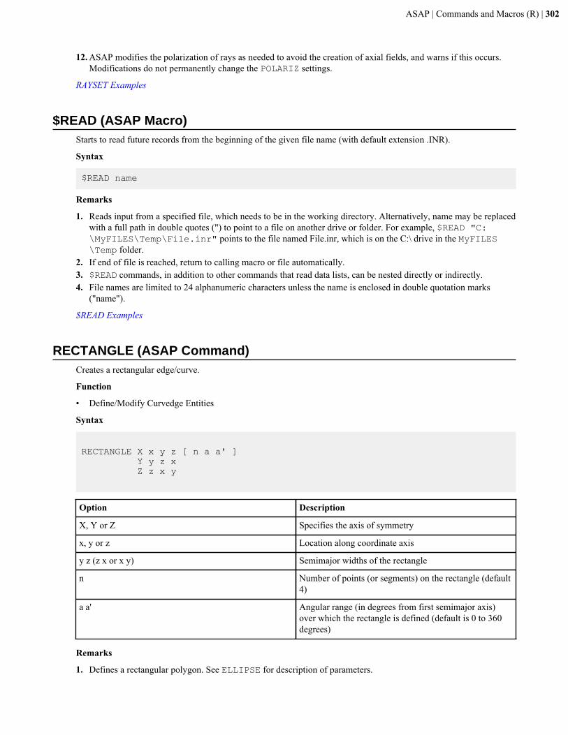
ASAP | Commands and Macros (R) | 302
12. ASAP modifies the polarization of rays as needed to avoid the creation of axial fields, and warns if this occurs.Modifications do not permanently change the POLARIZ settings.
RAYSET Examples
$READ (ASAP Macro)Starts to read future records from the beginning of the given file name (with default extension .INR).
Syntax
$READ name
Remarks
1. Reads input from a specified file, which needs to be in the working directory. Alternatively, name may be replacedwith a full path in double quotes (") to point to a file on another drive or folder. For example, $READ "C:\MyFILES\Temp\File.inr" points to the file named File.inr, which is on the C:\ drive in the MyFILES\Temp folder.
2. If end of file is reached, return to calling macro or file automatically.3. $READ commands, in addition to other commands that read data lists, can be nested directly or indirectly.4. File names are limited to 24 alphanumeric characters unless the name is enclosed in double quotation marks
("name").
$READ Examples
RECTANGLE (ASAP Command)Creates a rectangular edge/curve.
Function
• Define/Modify Curvedge Entities
Syntax
RECTANGLE X x y z [ n a a' ] Y y z x Z z x y
Option Description
X, Y or Z Specifies the axis of symmetry
x, y or z Location along coordinate axis
y z (z x or x y) Semimajor widths of the rectangle
n Number of points (or segments) on the rectangle (default4)
a a' Angular range (in degrees from first semimajor axis)over which the rectangle is defined (default is 0 to 360degrees)
Remarks
1. Defines a rectangular polygon. See ELLIPSE for description of parameters.
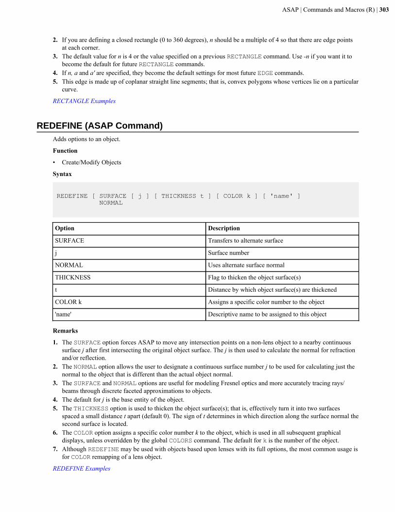
ASAP | Commands and Macros (R) | 303
2. If you are defining a closed rectangle (0 to 360 degrees), n should be a multiple of 4 so that there are edge pointsat each corner.
3. The default value for n is 4 or the value specified on a previous RECTANGLE command. Use -n if you want it tobecome the default for future RECTANGLE commands.
4. If n, a and a' are specified, they become the default settings for most future EDGE commands.5. This edge is made up of coplanar straight line segments; that is, convex polygons whose vertices lie on a particular
curve.
RECTANGLE Examples
REDEFINE (ASAP Command)Adds options to an object.
Function
• Create/Modify Objects
Syntax
REDEFINE [ SURFACE [ j ] [ THICKNESS t ] [ COLOR k ] [ 'name' ] NORMAL
Option Description
SURFACE Transfers to alternate surface
j Surface number
NORMAL Uses alternate surface normal
THICKNESS Flag to thicken the object surface(s)
t Distance by which object surface(s) are thickened
COLOR k Assigns a specific color number to the object
'name' Descriptive name to be assigned to this object
Remarks
1. The SURFACE option forces ASAP to move any intersection points on a non-lens object to a nearby continuoussurface j after first intersecting the original object surface. The j is then used to calculate the normal for refractionand/or reflection.
2. The NORMAL option allows the user to designate a continuous surface number j to be used for calculating just thenormal to the object that is different than the actual object normal.
3. The SURFACE and NORMAL options are useful for modeling Fresnel optics and more accurately tracing rays/beams through discrete faceted approximations to objects.
4. The default for j is the base entity of the object.5. The THICKNESS option is used to thicken the object surface(s); that is, effectively turn it into two surfaces
spaced a small distance t apart (default 0). The sign of t determines in which direction along the surface normal thesecond surface is located.
6. The COLOR option assigns a specific color number k to the object, which is used in all subsequent graphicaldisplays, unless overridden by the global COLORS command. The default for k is the number of the object.
7. Although REDEFINE may be used with objects based upon lenses with its full options, the most common usage isfor COLOR remapping of a lens object.
REDEFINE Examples
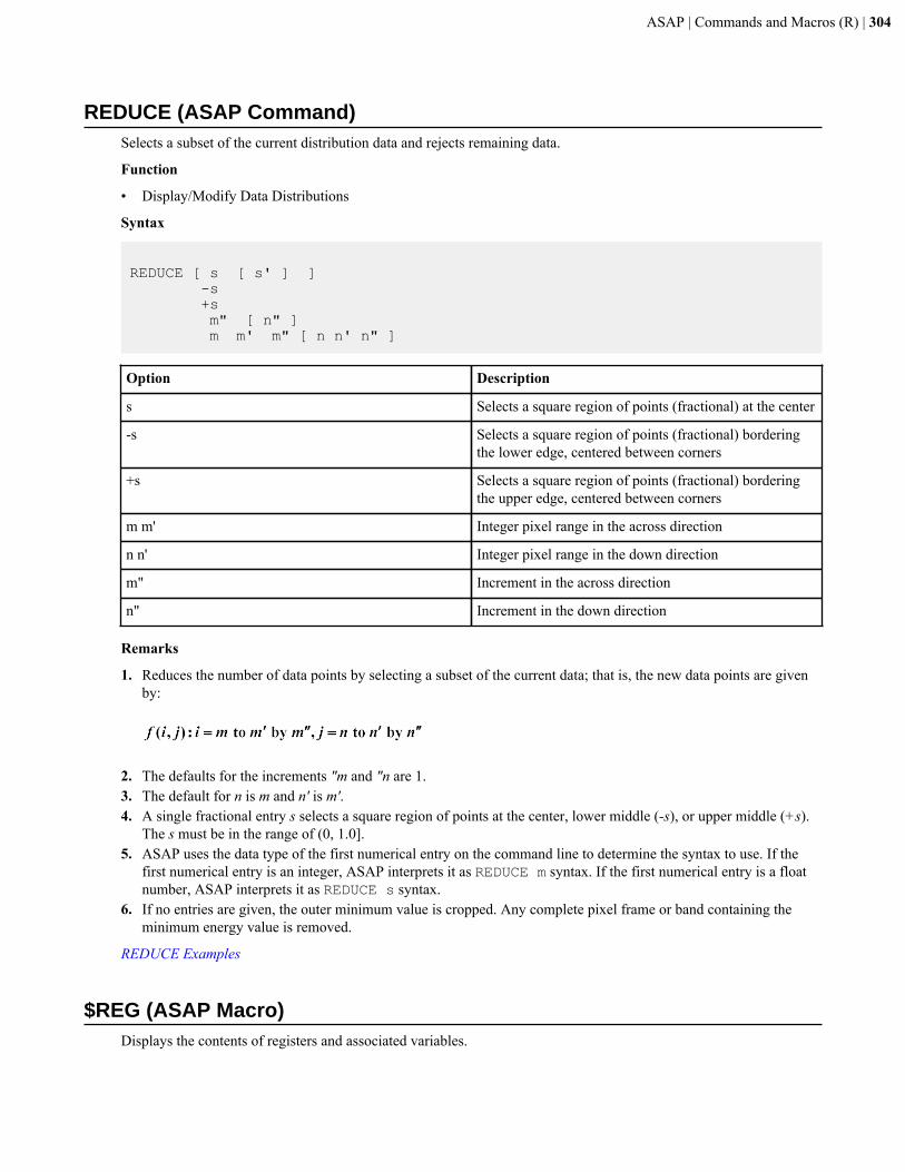
ASAP | Commands and Macros (R) | 304
REDUCE (ASAP Command)Selects a subset of the current distribution data and rejects remaining data.
Function
• Display/Modify Data Distributions
Syntax
REDUCE [ s [ s' ] ] -s +s m" [ n" ] m m' m" [ n n' n" ]
Option Description
s Selects a square region of points (fractional) at the center
-s Selects a square region of points (fractional) borderingthe lower edge, centered between corners
+s Selects a square region of points (fractional) borderingthe upper edge, centered between corners
m m' Integer pixel range in the across direction
n n' Integer pixel range in the down direction
m" Increment in the across direction
n" Increment in the down direction
Remarks
1. Reduces the number of data points by selecting a subset of the current data; that is, the new data points are givenby:
2. The defaults for the increments "m and "n are 1.3. The default for n is m and n' is m'.4. A single fractional entry s selects a square region of points at the center, lower middle (-s), or upper middle (+s).
The s must be in the range of (0, 1.0].5. ASAP uses the data type of the first numerical entry on the command line to determine the syntax to use. If the
first numerical entry is an integer, ASAP interprets it as REDUCE m syntax. If the first numerical entry is a floatnumber, ASAP interprets it as REDUCE s syntax.
6. If no entries are given, the outer minimum value is cropped. Any complete pixel frame or band containing theminimum energy value is removed.
REDUCE Examples
$REG (ASAP Macro)Displays the contents of registers and associated variables.

ASAP | Commands and Macros (R) | 305
Syntax
$REG [ register register' ... ] [ 'text' ]®
Remarks
1. Macro displays the contents of a given register or set of registers with optional 'text'2. If no registers or variables are entered, all the registers or variables for which content has changed since program
startup are displayed.3. $REG prints the internal ASAP register name in addition to the variable name(s) and value(s). ® prints only
the variable name(s) and value(s).
Examples
$REG Examples
REMOVE (ASAP Command)Subtracts best-fit polynomial.
Function
• Display/Modify Data Distributions
Syntax
REMOVE [ k ]
Option Description
k Degree of best-fit, 1D polynomial (default 1, linear)
Remarks
1. Removes (subtracts) best-fit, 1D polynomial of degree k from distribution data that is averaged in the otherdirection.
2. Takes the average of the data in the cross-direction and determines the best-fit polynomial of order k to thataveraged data. The best-fit polynomial is then subtracted from all rows and columns of the original data.
3. Use a TRANSPOSE and another REMOVE command to subtract a 2D polynomial (excluding any cross terms).
REMOVE Examples
RENDER (ASAP Command)Creates rendered graphics of the system geometry and ray trace.
Function
• Setup Plots and Verify System
Syntax
RENDER [ d ] [ DEPTH [ d' [ d"] ] ] [ RAYS [ s ] ] [MODEL [ m ] ] x y z
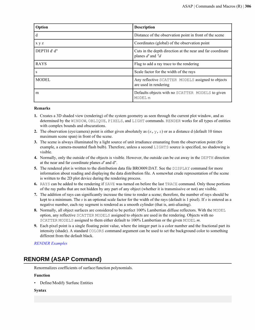
ASAP | Commands and Macros (R) | 306
Option Description
d Distance of the observation point in front of the scene
x y z Coordinates (global) of the observation point
DEPTH d' d" Cuts in the depth direction at the near and far coordinateplanes d' and "d
RAYS Flag to add a ray trace to the rendering
s Scale factor for the width of the rays
MODEL Any reflective SCATTER MODELS assigned to objectsare used in rendering
m Defaults objects with no SCATTER MODELS to givenMODEL m
Remarks
1. Creates a 3D shaded view (rendering) of the system geometry as seen through the current plot window, and asdetermined by the WINDOW, OBLIQUE, PIXELS, and LIGHT commands. RENDER works for all types of entitieswith complex bounds and obscurations.
2. The observation (eye/camera) point is either given absolutely as (x,y,z) or as a distance d (default 10 timesmaximum scene span) in front of the scene.
3. The scene is always illuminated by a light source of unit irradiance emanating from the observation point (forexample, a camera-mounted flash bulb). Therefore, unless a second LIGHTS source is specified, no shadowing isvisible.
4. Normally, only the outside of the objects is visible. However, the outside can be cut away in the DEPTH directionat the near and far coordinate planes d' and d".
5. The rendered plot is written to the distribution data file BRO009.DAT. See the DISPLAY command for moreinformation about reading and displaying the data distribution file. A somewhat crude representation of the sceneis written to the 2D plot device during the rendering process.
6. RAYS can be added to the rendering if SAVE was turned on before the last TRACE command. Only those portionsof the ray paths that are not hidden by any part of any object (whether it is transmissive or not) are visible.
7. The addition of rays can significantly increase the time to render a scene; therefore, the number of rays should bekept to a minimum. The s is an optional scale factor for the width of the rays (default is 1 pixel). If s is entered as anegative number, each ray segment is rendered as a smooth cylinder (that is, anti-aliasing).
8. Normally, all object surfaces are considered to be perfect 100% Lambertian diffuse reflectors. With the MODELoption, any reflective SCATTER MODELS assigned to objects are used in the rendering. Objects with noSCATTER MODELS assigned to them either default to 100% Lambertian or the given MODEL m.
9. Each pixel point is a single floating point value, where the integer part is a color number and the fractional part itsintensity (shade). A standard COLORS command argument can be used to set the background color to somethingdifferent from the default black.
RENDER Examples
RENORM (ASAP Command)Renormalizes coefficients of surface/function polynomials.
Function
• Define/Modify Surfunc Entities
Syntax
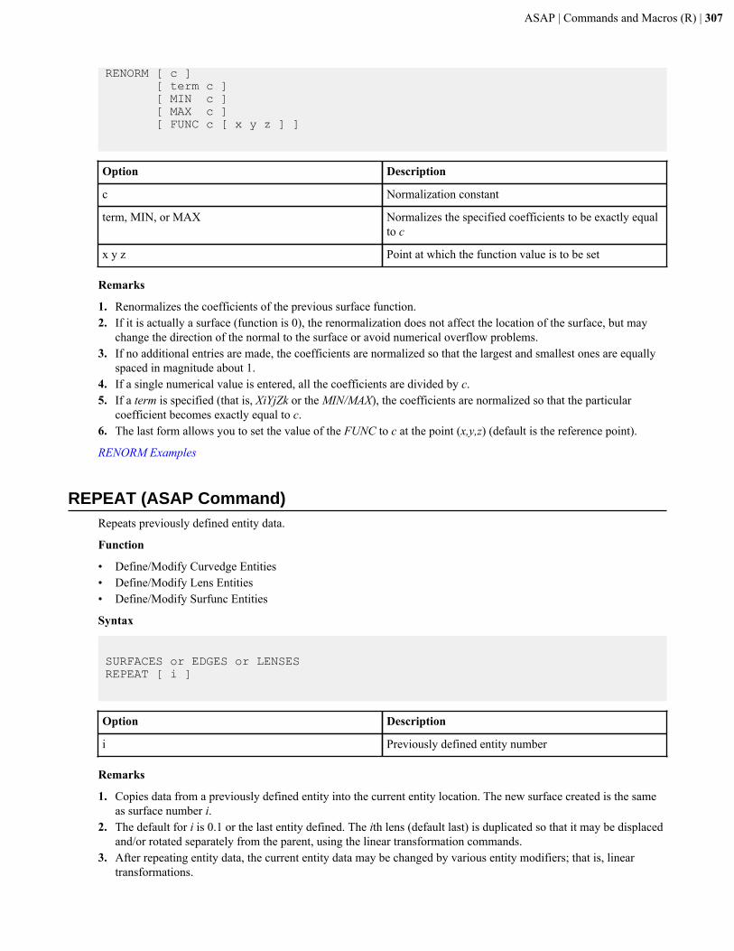
ASAP | Commands and Macros (R) | 307
RENORM [ c ] [ term c ] [ MIN c ] [ MAX c ] [ FUNC c [ x y z ] ]
Option Description
c Normalization constant
term, MIN, or MAX Normalizes the specified coefficients to be exactly equalto c
x y z Point at which the function value is to be set
Remarks
1. Renormalizes the coefficients of the previous surface function.2. If it is actually a surface (function is 0), the renormalization does not affect the location of the surface, but may
change the direction of the normal to the surface or avoid numerical overflow problems.3. If no additional entries are made, the coefficients are normalized so that the largest and smallest ones are equally
spaced in magnitude about 1.4. If a single numerical value is entered, all the coefficients are divided by c.5. If a term is specified (that is, XiYjZk or the MIN/MAX), the coefficients are normalized so that the particular
coefficient becomes exactly equal to c.6. The last form allows you to set the value of the FUNC to c at the point (x,y,z) (default is the reference point).
RENORM Examples
REPEAT (ASAP Command)Repeats previously defined entity data.
Function
• Define/Modify Curvedge Entities• Define/Modify Lens Entities• Define/Modify Surfunc Entities
Syntax
SURFACES or EDGES or LENSESREPEAT [ i ]
Option Description
i Previously defined entity number
Remarks
1. Copies data from a previously defined entity into the current entity location. The new surface created is the sameas surface number i.
2. The default for i is 0.1 or the last entity defined. The ith lens (default last) is duplicated so that it may be displacedand/or rotated separately from the parent, using the linear transformation commands.
3. After repeating entity data, the current entity data may be changed by various entity modifiers; that is, lineartransformations.
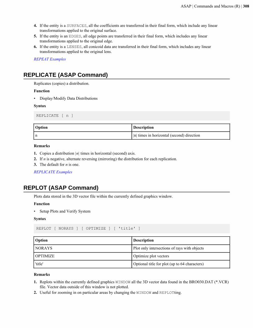
ASAP | Commands and Macros (R) | 308
4. If the entity is a SURFACES, all the coefficients are transferred in their final form, which include any lineartransformations applied to the original surface.
5. If the entity is an EDGES, all edge points are transferred in their final form, which includes any lineartransformations applied to the original edge.
6. If the entity is a LENSES, all conicoid data are transferred in their final form, which includes any lineartransformations applied to the original lens.
REPEAT Examples
REPLICATE (ASAP Command)Replicates (copies) a distribution.
Function
• Display/Modify Data Distributions
Syntax
REPLICATE [ n ]
Option Description
n |n| times in horizontal (second) direction
Remarks
1. Copies a distribution |n| times in horizontal (second) axis.2. If n is negative, alternate reversing (mirroring) the distribution for each replication.3. The default for n is one.
REPLICATE Examples
REPLOT (ASAP Command)Plots data stored in the 3D vector file within the currently defined graphics window.
Function
• Setup Plots and Verify System
Syntax
REPLOT [ NORAYS ] [ OPTIMIZE ] [ 'title' ]
Option Description
NORAYS Plot only intersections of rays with objects
OPTIMIZE Optimize plot vectors
'title' Optional title for plot (up to 64 characters)
Remarks
1. Replots within the currently defined graphics WINDOW all the 3D vector data found in the BRO030.DAT (*.VCR)file. Vector data outside of this window is not plotted.
2. Useful for zooming in on particular areas by changing the WINDOW and REPLOTting.
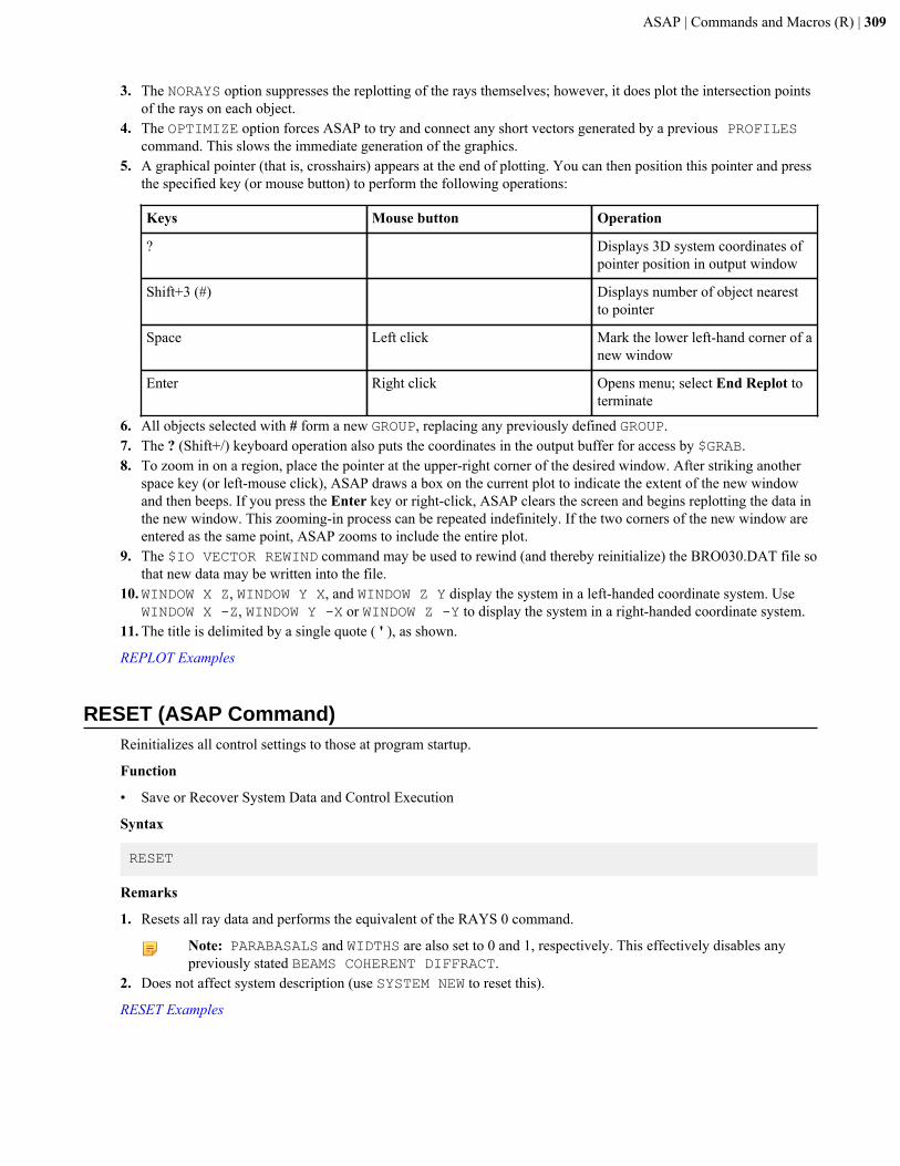
ASAP | Commands and Macros (R) | 309
3. The NORAYS option suppresses the replotting of the rays themselves; however, it does plot the intersection pointsof the rays on each object.
4. The OPTIMIZE option forces ASAP to try and connect any short vectors generated by a previous PROFILEScommand. This slows the immediate generation of the graphics.
5. A graphical pointer (that is, crosshairs) appears at the end of plotting. You can then position this pointer and pressthe specified key (or mouse button) to perform the following operations:
Keys Mouse button Operation
? Displays 3D system coordinates ofpointer position in output window
Shift+3 (#) Displays number of object nearestto pointer
Space Left click Mark the lower left-hand corner of anew window
Enter Right click Opens menu; select End Replot toterminate
6. All objects selected with # form a new GROUP, replacing any previously defined GROUP.7. The ? (Shift+/) keyboard operation also puts the coordinates in the output buffer for access by $GRAB.8. To zoom in on a region, place the pointer at the upper-right corner of the desired window. After striking another
space key (or left-mouse click), ASAP draws a box on the current plot to indicate the extent of the new windowand then beeps. If you press the Enter key or right-click, ASAP clears the screen and begins replotting the data inthe new window. This zooming-in process can be repeated indefinitely. If the two corners of the new window areentered as the same point, ASAP zooms to include the entire plot.
9. The $IO VECTOR REWIND command may be used to rewind (and thereby reinitialize) the BRO030.DAT file sothat new data may be written into the file.
10.WINDOW X Z, WINDOW Y X, and WINDOW Z Y display the system in a left-handed coordinate system. UseWINDOW X -Z, WINDOW Y -X or WINDOW Z -Y to display the system in a right-handed coordinate system.
11. The title is delimited by a single quote ( ' ), as shown.
REPLOT Examples
RESET (ASAP Command)Reinitializes all control settings to those at program startup.
Function
• Save or Recover System Data and Control Execution
Syntax
RESET
Remarks
1. Resets all ray data and performs the equivalent of the RAYS 0 command.
Note: PARABASALS and WIDTHS are also set to 0 and 1, respectively. This effectively disables anypreviously stated BEAMS COHERENT DIFFRACT.
2. Does not affect system description (use SYSTEM NEW to reset this).
RESET Examples
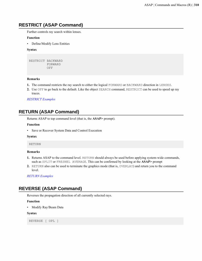
ASAP | Commands and Macros (R) | 310
RESTRICT (ASAP Command)Further controls ray search within lenses.
Function
• Define/Modify Lens Entities
Syntax
RESTRICT BACKWARD FORWARD OFF
Remarks
1. The command restricts the ray search to either the logical FORWARD or BACKWARD direction in LENSES.2. Use OFF to go back to the default. Like the object SEARCH command, RESTRICT can be used to speed up ray
traces.
RESTRICT Examples
RETURN (ASAP Command)Returns ASAP to top command level (that is, the ASAP> prompt).
Function
• Save or Recover System Data and Control Execution
Syntax
RETURN
Remarks
1. Returns ASAP to the command level. RETURN should always be used before applying system-wide commands,such as SPLIT or FRESNEL AVERAGE. This can be confirmed by looking at the ASAP> prompt
2. RETURN also can be used to terminate the graphics mode (that is, OVERLAY) and return you to the commandlevel.
RETURN Examples
REVERSE (ASAP Command)Reverses the propagation direction of all currently selected rays.
Function
• Modify Ray/Beam Data
Syntax
REVERSE [ OPL ]
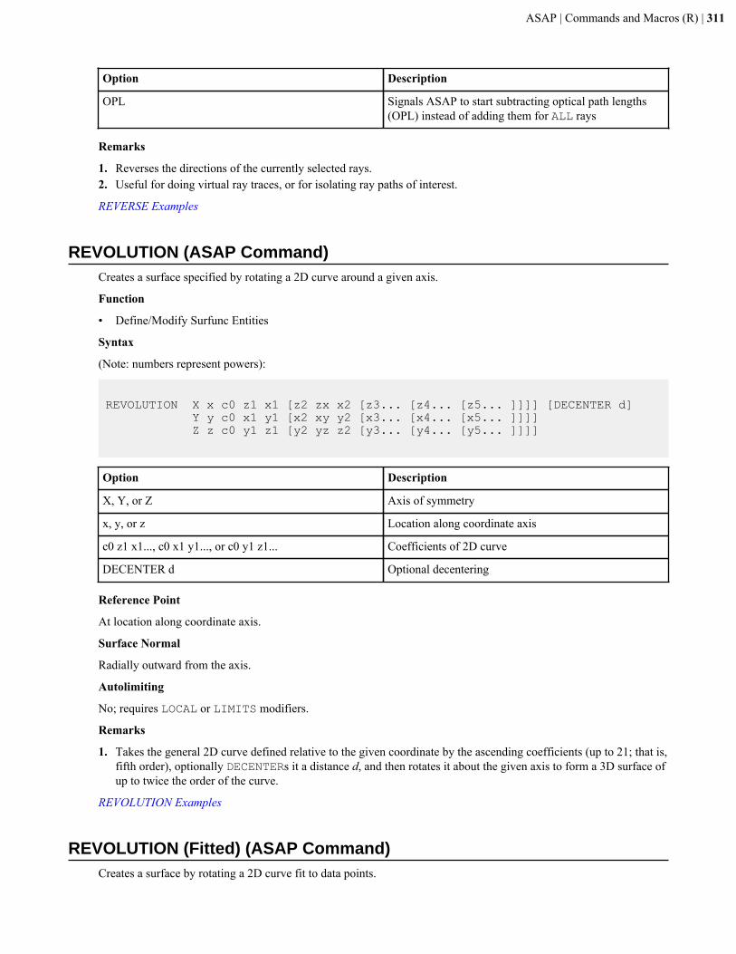
ASAP | Commands and Macros (R) | 311
Option Description
OPL Signals ASAP to start subtracting optical path lengths(OPL) instead of adding them for ALL rays
Remarks
1. Reverses the directions of the currently selected rays.2. Useful for doing virtual ray traces, or for isolating ray paths of interest.
REVERSE Examples
REVOLUTION (ASAP Command)Creates a surface specified by rotating a 2D curve around a given axis.
Function
• Define/Modify Surfunc Entities
Syntax
(Note: numbers represent powers):
REVOLUTION X x c0 z1 x1 [z2 zx x2 [z3... [z4... [z5... ]]]] [DECENTER d] Y y c0 x1 y1 [x2 xy y2 [x3... [x4... [x5... ]]]] Z z c0 y1 z1 [y2 yz z2 [y3... [y4... [y5... ]]]]
Option Description
X, Y, or Z Axis of symmetry
x, y, or z Location along coordinate axis
c0 z1 x1..., c0 x1 y1..., or c0 y1 z1... Coefficients of 2D curve
DECENTER d Optional decentering
Reference Point
At location along coordinate axis.
Surface Normal
Radially outward from the axis.
Autolimiting
No; requires LOCAL or LIMITS modifiers.
Remarks
1. Takes the general 2D curve defined relative to the given coordinate by the ascending coefficients (up to 21; that is,fifth order), optionally DECENTERs it a distance d, and then rotates it about the given axis to form a 3D surface ofup to twice the order of the curve.
REVOLUTION Examples
REVOLUTION (Fitted) (ASAP Command)Creates a surface by rotating a 2D curve fit to data points.
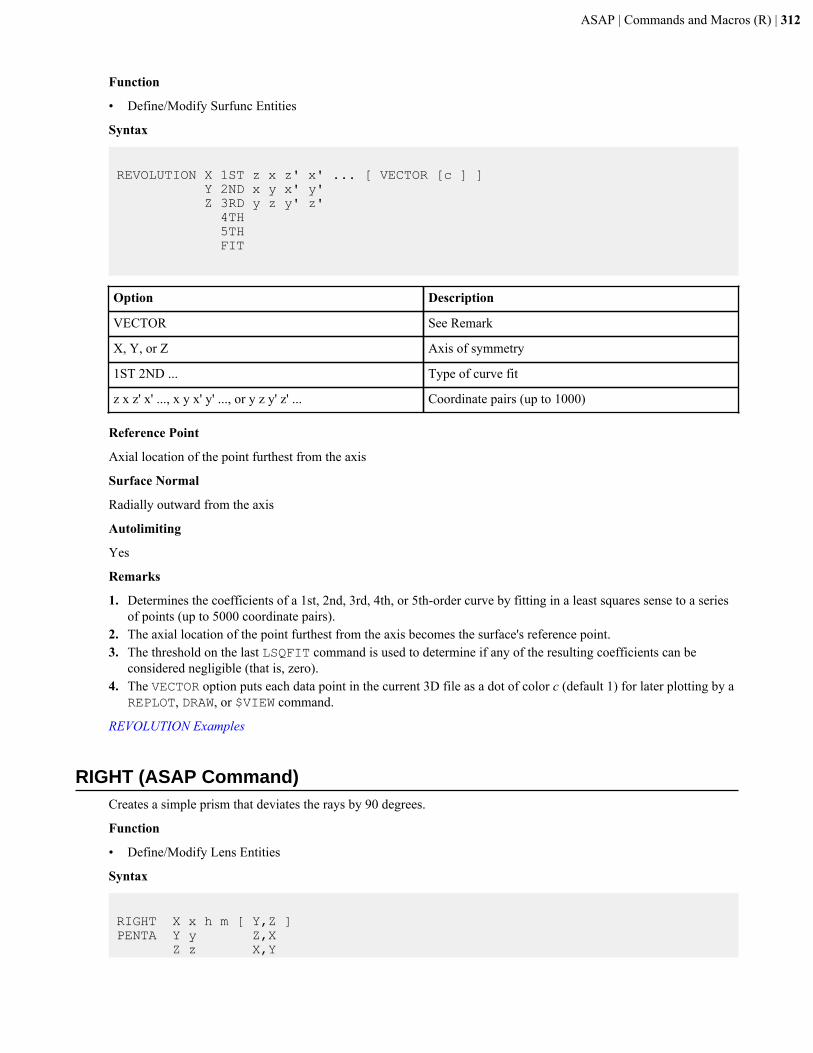
ASAP | Commands and Macros (R) | 312
Function
• Define/Modify Surfunc Entities
Syntax
REVOLUTION X 1ST z x z' x' ... [ VECTOR [c ] ] Y 2ND x y x' y' Z 3RD y z y' z' 4TH 5TH FIT
Option Description
VECTOR See Remark
X, Y, or Z Axis of symmetry
1ST 2ND ... Type of curve fit
z x z' x' ..., x y x' y' ..., or y z y' z' ... Coordinate pairs (up to 1000)
Reference Point
Axial location of the point furthest from the axis
Surface Normal
Radially outward from the axis
Autolimiting
Yes
Remarks
1. Determines the coefficients of a 1st, 2nd, 3rd, 4th, or 5th-order curve by fitting in a least squares sense to a seriesof points (up to 5000 coordinate pairs).
2. The axial location of the point furthest from the axis becomes the surface's reference point.3. The threshold on the last LSQFIT command is used to determine if any of the resulting coefficients can be
considered negligible (that is, zero).4. The VECTOR option puts each data point in the current 3D file as a dot of color c (default 1) for later plotting by a
REPLOT, DRAW, or $VIEW command.
REVOLUTION Examples
RIGHT (ASAP Command)Creates a simple prism that deviates the rays by 90 degrees.
Function
• Define/Modify Lens Entities
Syntax
RIGHT X x h m [ Y,Z ]PENTA Y y Z,X Z z X,Y
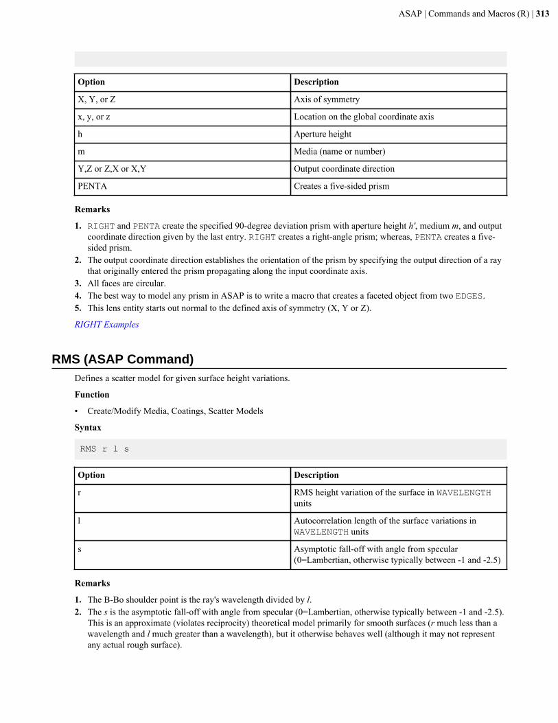
ASAP | Commands and Macros (R) | 313
Option Description
X, Y, or Z Axis of symmetry
x, y, or z Location on the global coordinate axis
h Aperture height
m Media (name or number)
Y,Z or Z,X or X,Y Output coordinate direction
PENTA Creates a five-sided prism
Remarks
1. RIGHT and PENTA create the specified 90-degree deviation prism with aperture height h', medium m, and outputcoordinate direction given by the last entry. RIGHT creates a right-angle prism; whereas, PENTA creates a five-sided prism.
2. The output coordinate direction establishes the orientation of the prism by specifying the output direction of a raythat originally entered the prism propagating along the input coordinate axis.
3. All faces are circular.4. The best way to model any prism in ASAP is to write a macro that creates a faceted object from two EDGES.5. This lens entity starts out normal to the defined axis of symmetry (X, Y or Z).
RIGHT Examples
RMS (ASAP Command)Defines a scatter model for given surface height variations.
Function
• Create/Modify Media, Coatings, Scatter Models
Syntax
RMS r l s
Option Description
r RMS height variation of the surface in WAVELENGTHunits
l Autocorrelation length of the surface variations inWAVELENGTH units
s Asymptotic fall-off with angle from specular(0=Lambertian, otherwise typically between -1 and -2.5)
Remarks
1. The B-Bo shoulder point is the ray's wavelength divided by l.2. The s is the asymptotic fall-off with angle from specular (0=Lambertian, otherwise typically between -1 and -2.5).
This is an approximate (violates reciprocity) theoretical model primarily for smooth surfaces (r much less than awavelength and l much greater than a wavelength), but it otherwise behaves well (although it may not representany actual rough surface).

ASAP | Commands and Macros (R) | 314
3. The BSDF varies with wavelength, incidence direction, scatter direction, and the specific object's INTERFACEproperties. It also automatically conserves energy (within standard statistical variations) if a ROUGHNESS r lcommand is also assigned to the object.
RMS Examples
ROOF (ASAP Command)Two rectangles that are "hinged" at a common side.
Function
• Define/Modify Surfunc Entities
Syntax
ROOF X x y [ z [ a ] ] Y y z x Z z x y
Remarks
1. Two rectangles with a (nearly) common edge at the given location, and with an apex angle a in degrees (default90) between them.
2. The "base" of the roof (which is perpendicular to the given AXIS) has semiwidths specified by the third andfourth entries.
3. A small gap exists between the rectangles, because they must be represented by a single, implicit equation, and thenormal is undefined there.
ROOF Examples
ROTATE (ASAP Command)Rotates an entity, object, or source about a point.
Function
• Create/Modify Objects• Define/Modify Curvedge Entities• Define/Modify Lens Entities• Define/Modify Surfunc Entities• Modify Ray/Beam Data
Syntax 1
ROTATE X d [ y z ] [ LIST ] Y d z x Z d x y
Syntax 2
ROTATE d ABOUT a,b,c [ x y z ] [ LIST ]
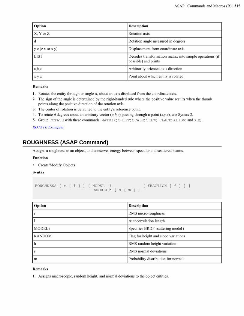
ASAP | Commands and Macros (R) | 315
Option Description
X, Y or Z Rotation axis
d Rotation angle measured in degrees
y z (z x or x y) Displacement from coordinate axis
LIST Decodes transformation matrix into simple operations (ifpossible) and prints
a,b,c Arbitrarily oriented axis direction
x y z Point about which entity is rotated
Remarks
1. Rotates the entity through an angle d, about an axis displaced from the coordinate axis.2. The sign of the angle is determined by the right-handed rule where the positive value results when the thumb
points along the positive direction of the rotation axis.3. The center of rotation is defaulted to the entity's reference point.4. To rotate d degrees about an arbitrary vector (a,b,c) passing through a point (x,y,z), use Syntax 2.5. Group ROTATE with these commands: MATRIX; SHIFT; SCALE; SKEW; PLACE; ALIGN; and XEQ.
ROTATE Examples
ROUGHNESS (ASAP Command)Assigns a roughness to an object, and conserves energy between specular and scattered beams.
Function
• Create/Modify Objects
Syntax
ROUGHNESS [ r [ l ] ] [ MODEL i [ FRACTION [ f ] ] ] RANDOM h [ s [ m ] ]
Option Description
r RMS micro-roughness
l Autocorrelation length
MODEL i Specifies BRDF scattering model i
RANDOM Flag for height and slope variations
h RMS random height variation
s RMS normal deviations
m Probability distribution for normal
Remarks
1. Assigns macroscopic, random height, and normal deviations to the object entities.
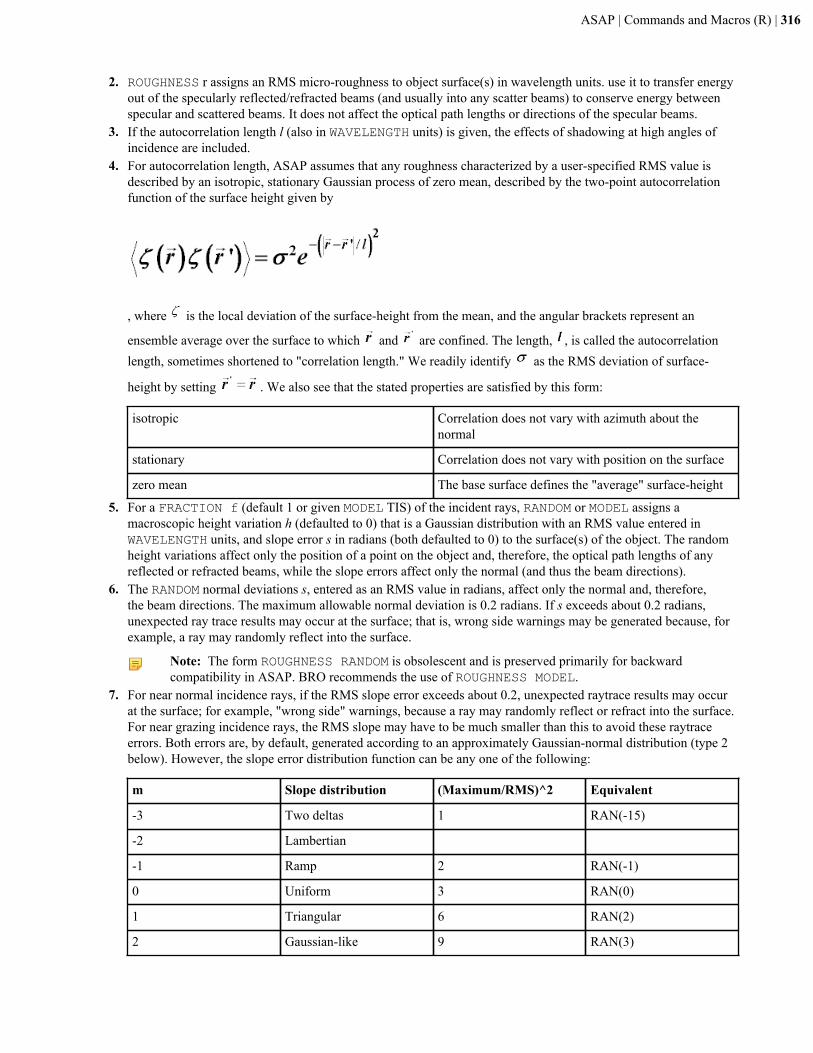
ASAP | Commands and Macros (R) | 316
2. ROUGHNESS r assigns an RMS micro-roughness to object surface(s) in wavelength units. use it to transfer energyout of the specularly reflected/refracted beams (and usually into any scatter beams) to conserve energy betweenspecular and scattered beams. It does not affect the optical path lengths or directions of the specular beams.
3. If the autocorrelation length l (also in WAVELENGTH units) is given, the effects of shadowing at high angles ofincidence are included.
4. For autocorrelation length, ASAP assumes that any roughness characterized by a user-specified RMS value isdescribed by an isotropic, stationary Gaussian process of zero mean, described by the two-point autocorrelationfunction of the surface height given by
, where is the local deviation of the surface-height from the mean, and the angular brackets represent an
ensemble average over the surface to which and are confined. The length, , is called the autocorrelationlength, sometimes shortened to "correlation length." We readily identify as the RMS deviation of surface-
height by setting . We also see that the stated properties are satisfied by this form:
isotropic Correlation does not vary with azimuth about thenormal
stationary Correlation does not vary with position on the surface
zero mean The base surface defines the "average" surface-height
5. For a FRACTION f (default 1 or given MODEL TIS) of the incident rays, RANDOM or MODEL assigns amacroscopic height variation h (defaulted to 0) that is a Gaussian distribution with an RMS value entered inWAVELENGTH units, and slope error s in radians (both defaulted to 0) to the surface(s) of the object. The randomheight variations affect only the position of a point on the object and, therefore, the optical path lengths of anyreflected or refracted beams, while the slope errors affect only the normal (and thus the beam directions).
6. The RANDOM normal deviations s, entered as an RMS value in radians, affect only the normal and, therefore,the beam directions. The maximum allowable normal deviation is 0.2 radians. If s exceeds about 0.2 radians,unexpected ray trace results may occur at the surface; that is, wrong side warnings may be generated because, forexample, a ray may randomly reflect into the surface.
Note: The form ROUGHNESS RANDOM is obsolescent and is preserved primarily for backwardcompatibility in ASAP. BRO recommends the use of ROUGHNESS MODEL.
7. For near normal incidence rays, if the RMS slope error exceeds about 0.2, unexpected raytrace results may occurat the surface; for example, "wrong side" warnings, because a ray may randomly reflect or refract into the surface.For near grazing incidence rays, the RMS slope may have to be much smaller than this to avoid these raytraceerrors. Both errors are, by default, generated according to an approximately Gaussian-normal distribution (type 2below). However, the slope error distribution function can be any one of the following:
m Slope distribution (Maximum/RMS)^2 Equivalent
-3 Two deltas 1 RAN(-15)
-2 Lambertian
-1 Ramp 2 RAN(-1)
0 Uniform 3 RAN(0)
1 Triangular 6 RAN(2)
2 Gaussian-like 9 RAN(3)
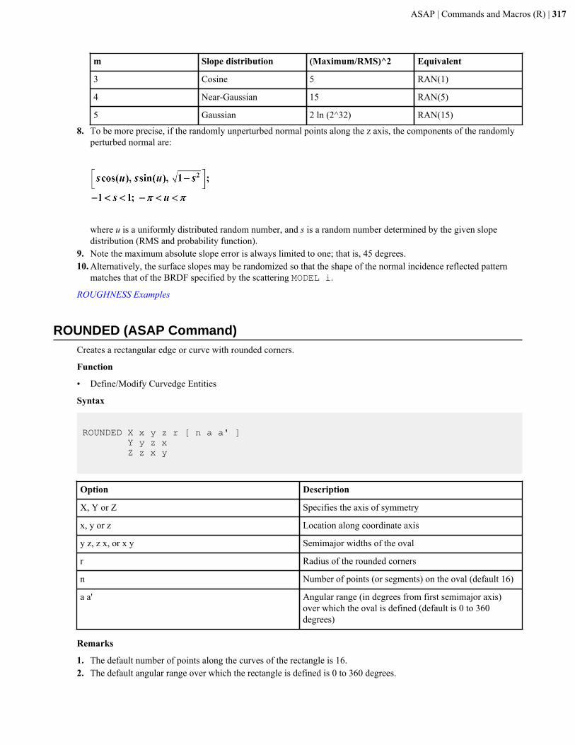
ASAP | Commands and Macros (R) | 317
m Slope distribution (Maximum/RMS)^2 Equivalent
3 Cosine 5 RAN(1)
4 Near-Gaussian 15 RAN(5)
5 Gaussian 2 ln (2^32) RAN(15)
8. To be more precise, if the randomly unperturbed normal points along the z axis, the components of the randomlyperturbed normal are:
where u is a uniformly distributed random number, and s is a random number determined by the given slopedistribution (RMS and probability function).
9. Note the maximum absolute slope error is always limited to one; that is, 45 degrees.10. Alternatively, the surface slopes may be randomized so that the shape of the normal incidence reflected pattern
matches that of the BRDF specified by the scattering MODEL i.
ROUGHNESS Examples
ROUNDED (ASAP Command)Creates a rectangular edge or curve with rounded corners.
Function
• Define/Modify Curvedge Entities
Syntax
ROUNDED X x y z r [ n a a' ] Y y z x Z z x y
Option Description
X, Y or Z Specifies the axis of symmetry
x, y or z Location along coordinate axis
y z, z x, or x y Semimajor widths of the oval
r Radius of the rounded corners
n Number of points (or segments) on the oval (default 16)
a a' Angular range (in degrees from first semimajor axis)over which the oval is defined (default is 0 to 360degrees)
Remarks
1. The default number of points along the curves of the rectangle is 16.2. The default angular range over which the rectangle is defined is 0 to 360 degrees.
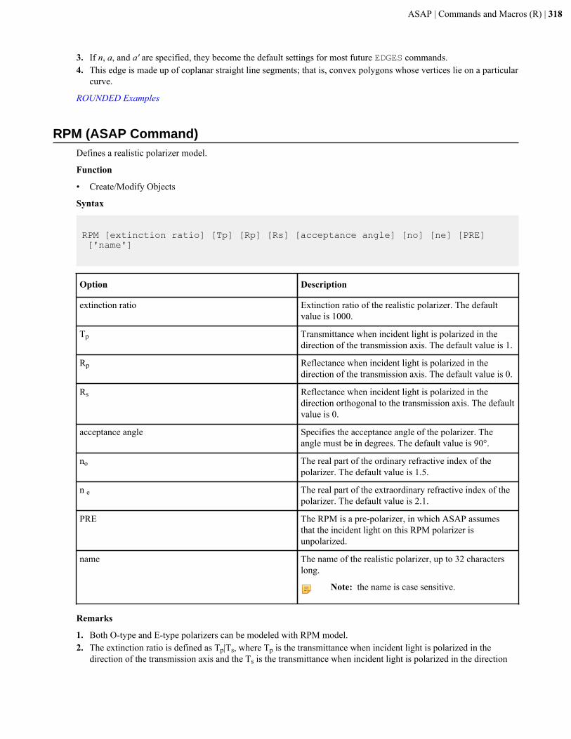
ASAP | Commands and Macros (R) | 318
3. If n, a, and a' are specified, they become the default settings for most future EDGES commands.4. This edge is made up of coplanar straight line segments; that is, convex polygons whose vertices lie on a particular
curve.
ROUNDED Examples
RPM (ASAP Command)Defines a realistic polarizer model.
Function
• Create/Modify Objects
Syntax
RPM [extinction ratio] [Tp] [Rp] [Rs] [acceptance angle] [no] [ne] [PRE] ['name']
Option Description
extinction ratio Extinction ratio of the realistic polarizer. The defaultvalue is 1000.
Tp Transmittance when incident light is polarized in thedirection of the transmission axis. The default value is 1.
Rp Reflectance when incident light is polarized in thedirection of the transmission axis. The default value is 0.
Rs Reflectance when incident light is polarized in thedirection orthogonal to the transmission axis. The defaultvalue is 0.
acceptance angle Specifies the acceptance angle of the polarizer. Theangle must be in degrees. The default value is 90°.
no The real part of the ordinary refractive index of thepolarizer. The default value is 1.5.
n e The real part of the extraordinary refractive index of thepolarizer. The default value is 2.1.
PRE The RPM is a pre-polarizer, in which ASAP assumesthat the incident light on this RPM polarizer isunpolarized.
name The name of the realistic polarizer, up to 32 characterslong.
Note: the name is case sensitive.
Remarks
1. Both O-type and E-type polarizers can be modeled with RPM model.2. The extinction ratio is defined as Tp|Ts, where Tp is the transmittance when incident light is polarized in the
direction of the transmission axis and the Ts is the transmittance when incident light is polarized in the direction
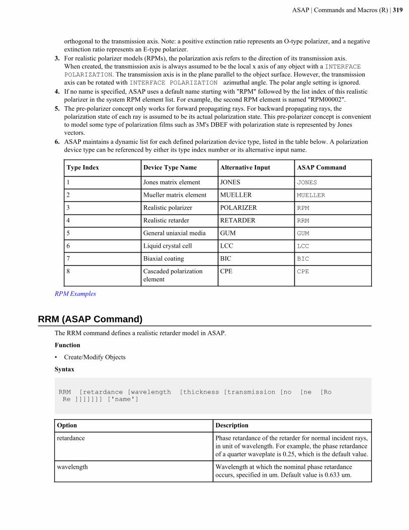
ASAP | Commands and Macros (R) | 319
orthogonal to the transmission axis. Note: a positive extinction ratio represents an O-type polarizer, and a negativeextinction ratio represents an E-type polarizer.
3. For realistic polarizer models (RPMs), the polarization axis refers to the direction of its transmission axis.When created, the transmission axis is always assumed to be the local x axis of any object with a INTERFACEPOLARIZATION. The transmission axis is in the plane parallel to the object surface. However, the transmissionaxis can be rotated with INTERFACE POLARIZATION azimuthal angle. The polar angle setting is ignored.
4. If no name is specified, ASAP uses a default name starting with "RPM" followed by the list index of this realisticpolarizer in the system RPM element list. For example, the second RPM element is named "RPM00002".
5. The pre-polarizer concept only works for forward propagating rays. For backward propagating rays, thepolarization state of each ray is assumed to be its actual polarization state. This pre-polarizer concept is convenientto model some type of polarization films such as 3M's DBEF with polarization state is represented by Jonesvectors.
6. ASAP maintains a dynamic list for each defined polarization device type, listed in the table below. A polarizationdevice type can be referenced by either its type index number or its alternative input name.
Type Index Device Type Name Alternative Input ASAP Command
1 Jones matrix element JONES JONES
2 Mueller matrix element MUELLER MUELLER
3 Realistic polarizer POLARIZER RPM
4 Realistic retarder RETARDER RRM
5 General uniaxial media GUM GUM
6 Liquid crystal cell LCC LCC
7 Biaxial coating BIC BIC
8 Cascaded polarizationelement
CPE CPE
RPM Examples
RRM (ASAP Command)The RRM command defines a realistic retarder model in ASAP.
Function
• Create/Modify Objects
Syntax
RRM [retardance [wavelength [thickness [transmission [no [ne [Ro Re ]]]]]]] ['name']
Option Description
retardance Phase retardance of the retarder for normal incident rays,in unit of wavelength. For example, the phase retardanceof a quarter waveplate is 0.25, which is the default value.
wavelength Wavelength at which the nominal phase retardanceoccurs, specified in um. Default value is 0.633 um.
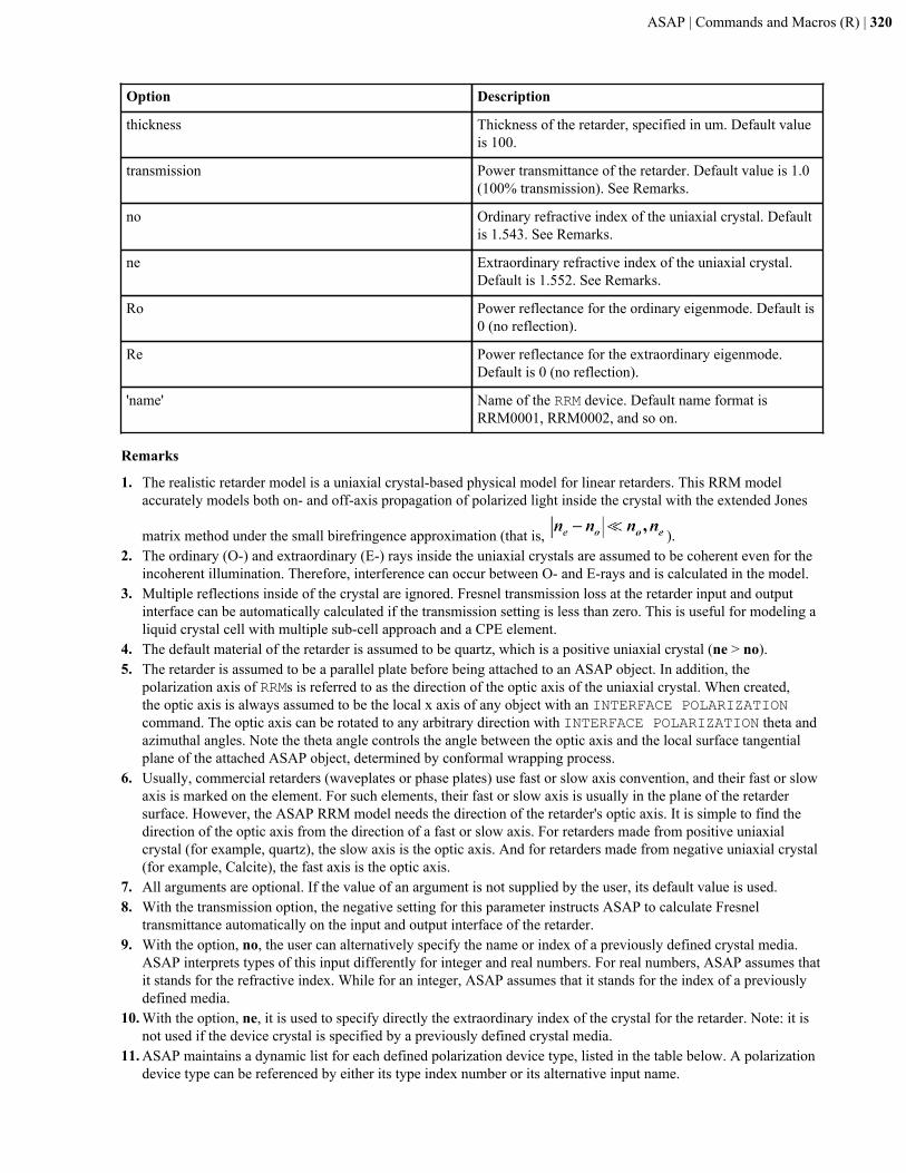
ASAP | Commands and Macros (R) | 320
Option Description
thickness Thickness of the retarder, specified in um. Default valueis 100.
transmission Power transmittance of the retarder. Default value is 1.0(100% transmission). See Remarks.
no Ordinary refractive index of the uniaxial crystal. Defaultis 1.543. See Remarks.
ne Extraordinary refractive index of the uniaxial crystal.Default is 1.552. See Remarks.
Ro Power reflectance for the ordinary eigenmode. Default is0 (no reflection).
Re Power reflectance for the extraordinary eigenmode.Default is 0 (no reflection).
'name' Name of the RRM device. Default name format isRRM0001, RRM0002, and so on.
Remarks
1. The realistic retarder model is a uniaxial crystal-based physical model for linear retarders. This RRM modelaccurately models both on- and off-axis propagation of polarized light inside the crystal with the extended Jones
matrix method under the small birefringence approximation (that is, ).2. The ordinary (O-) and extraordinary (E-) rays inside the uniaxial crystals are assumed to be coherent even for the
incoherent illumination. Therefore, interference can occur between O- and E-rays and is calculated in the model.3. Multiple reflections inside of the crystal are ignored. Fresnel transmission loss at the retarder input and output
interface can be automatically calculated if the transmission setting is less than zero. This is useful for modeling aliquid crystal cell with multiple sub-cell approach and a CPE element.
4. The default material of the retarder is assumed to be quartz, which is a positive uniaxial crystal (ne > no).5. The retarder is assumed to be a parallel plate before being attached to an ASAP object. In addition, the
polarization axis of RRMs is referred to as the direction of the optic axis of the uniaxial crystal. When created,the optic axis is always assumed to be the local x axis of any object with an INTERFACE POLARIZATIONcommand. The optic axis can be rotated to any arbitrary direction with INTERFACE POLARIZATION theta andazimuthal angles. Note the theta angle controls the angle between the optic axis and the local surface tangentialplane of the attached ASAP object, determined by conformal wrapping process.
6. Usually, commercial retarders (waveplates or phase plates) use fast or slow axis convention, and their fast or slowaxis is marked on the element. For such elements, their fast or slow axis is usually in the plane of the retardersurface. However, the ASAP RRM model needs the direction of the retarder's optic axis. It is simple to find thedirection of the optic axis from the direction of a fast or slow axis. For retarders made from positive uniaxialcrystal (for example, quartz), the slow axis is the optic axis. And for retarders made from negative uniaxial crystal(for example, Calcite), the fast axis is the optic axis.
7. All arguments are optional. If the value of an argument is not supplied by the user, its default value is used.8. With the transmission option, the negative setting for this parameter instructs ASAP to calculate Fresnel
transmittance automatically on the input and output interface of the retarder.9. With the option, no, the user can alternatively specify the name or index of a previously defined crystal media.
ASAP interprets types of this input differently for integer and real numbers. For real numbers, ASAP assumes thatit stands for the refractive index. While for an integer, ASAP assumes that it stands for the index of a previouslydefined media.
10. With the option, ne, it is used to specify directly the extraordinary index of the crystal for the retarder. Note: it isnot used if the device crystal is specified by a previously defined crystal media.
11. ASAP maintains a dynamic list for each defined polarization device type, listed in the table below. A polarizationdevice type can be referenced by either its type index number or its alternative input name.
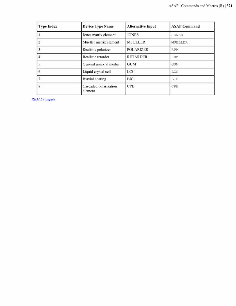
ASAP | Commands and Macros (R) | 321
Type Index Device Type Name Alternative Input ASAP Command
1 Jones matrix element JONES JONES
2 Mueller matrix element MUELLER MUELLER
3 Realistic polarizer POLARIZER RPM
4 Realistic retarder RETARDER RRM
5 General uniaxial media GUM GUM
6 Liquid crystal cell LCC LCC
7 Biaxial coating BIC BIC
8 Cascaded polarizationelement
CPE CPE
RRM Examples
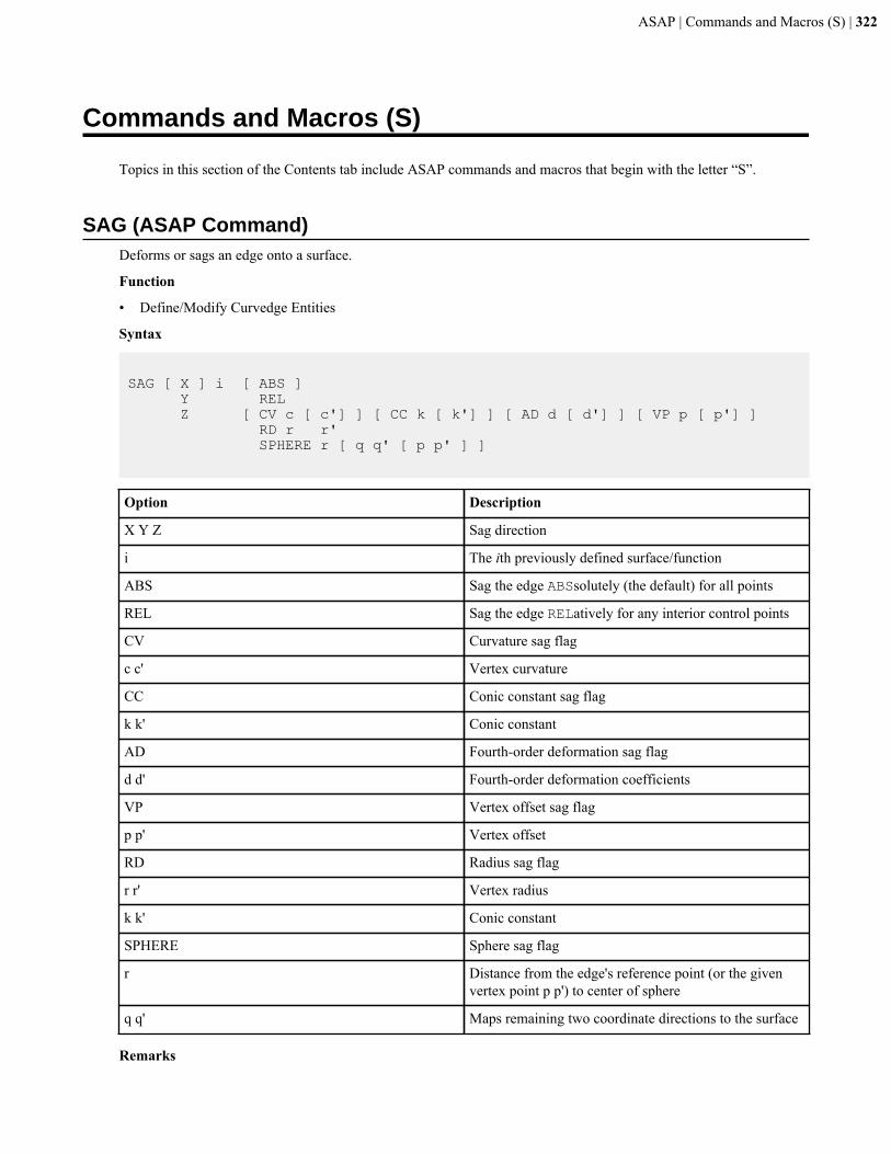
ASAP | Commands and Macros (S) | 322
Commands and Macros (S)
Topics in this section of the Contents tab include ASAP commands and macros that begin with the letter “S”.
SAG (ASAP Command)Deforms or sags an edge onto a surface.
Function
• Define/Modify Curvedge Entities
Syntax
SAG [ X ] i [ ABS ] Y REL Z [ CV c [ c'] ] [ CC k [ k'] ] [ AD d [ d'] ] [ VP p [ p'] ] RD r r' SPHERE r [ q q' [ p p' ] ]
Option Description
X Y Z Sag direction
i The ith previously defined surface/function
ABS Sag the edge ABSsolutely (the default) for all points
REL Sag the edge RELatively for any interior control points
CV Curvature sag flag
c c' Vertex curvature
CC Conic constant sag flag
k k' Conic constant
AD Fourth-order deformation sag flag
d d' Fourth-order deformation coefficients
VP Vertex offset sag flag
p p' Vertex offset
RD Radius sag flag
r r' Vertex radius
k k' Conic constant
SPHERE Sphere sag flag
r Distance from the edge's reference point (or the givenvertex point p p') to center of sphere
q q' Maps remaining two coordinate directions to the surface
Remarks
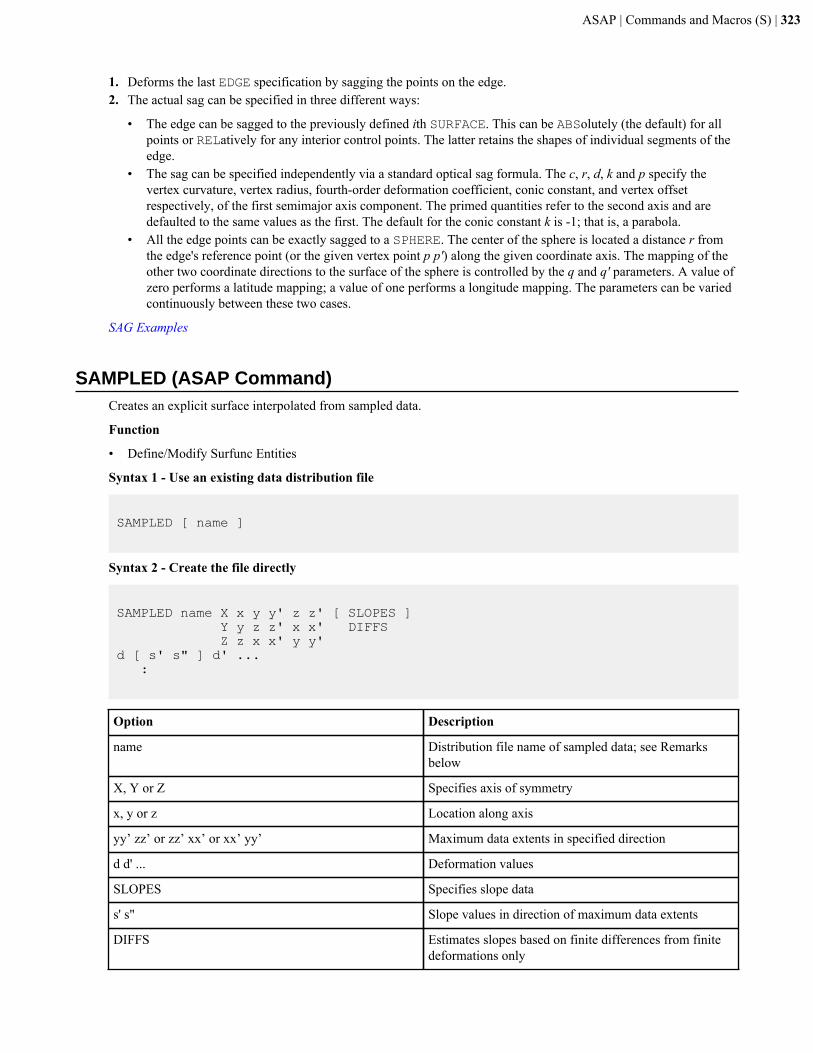
ASAP | Commands and Macros (S) | 323
1. Deforms the last EDGE specification by sagging the points on the edge.2. The actual sag can be specified in three different ways:
• The edge can be sagged to the previously defined ith SURFACE. This can be ABSolutely (the default) for allpoints or RELatively for any interior control points. The latter retains the shapes of individual segments of theedge.
• The sag can be specified independently via a standard optical sag formula. The c, r, d, k and p specify thevertex curvature, vertex radius, fourth-order deformation coefficient, conic constant, and vertex offsetrespectively, of the first semimajor axis component. The primed quantities refer to the second axis and aredefaulted to the same values as the first. The default for the conic constant k is -1; that is, a parabola.
• All the edge points can be exactly sagged to a SPHERE. The center of the sphere is located a distance r fromthe edge's reference point (or the given vertex point p p') along the given coordinate axis. The mapping of theother two coordinate directions to the surface of the sphere is controlled by the q and q' parameters. A value ofzero performs a latitude mapping; a value of one performs a longitude mapping. The parameters can be variedcontinuously between these two cases.
SAG Examples
SAMPLED (ASAP Command)Creates an explicit surface interpolated from sampled data.
Function
• Define/Modify Surfunc Entities
Syntax 1 - Use an existing data distribution file
SAMPLED [ name ]
Syntax 2 - Create the file directly
SAMPLED name X x y y' z z' [ SLOPES ] Y y z z' x x' DIFFS Z z x x' y y'd [ s' s" ] d' ... :
Option Description
name Distribution file name of sampled data; see Remarksbelow
X, Y or Z Specifies axis of symmetry
x, y or z Location along axis
yy’ zz’ or zz’ xx’ or xx’ yy’ Maximum data extents in specified direction
d d' ... Deformation values
SLOPES Specifies slope data
s' s" Slope values in direction of maximum data extents
DIFFS Estimates slopes based on finite differences from finitedeformations only
ASAP | Commands and Macros (S) | 324
Reference Point
If read from a distribution file, name.dis file (default BRO009.DAT), point is at (0,0) depth coordinate.
If created directly, point is at the intersection of reference plane and coordinate axis.
Surface Normal
Along positive coordinate direction
Autolimiting
Yes, see Remarks
Remarks
1. Creates an explicit surface defined by:
• Reading deformation samples found in the binary distribution file name.dis (default BRO009.DAT) externalfile.
• Entering the sample points following the command description.2. The deformation and slopes for ray tracing, if specified in the distribution file, are linearly interpolated between
data points. Up to 1000 data points are allowed in the across direction and an unlimited number in the downdirection.
3. Each directly created SAMPLED surface must be given a distinct distribution file name.
WARNING: Attempts to re-use a distribution file name for directly created SAMPLED data results in an error.ASAP generates the error message, "The named distribution file already exists." ASAP does not crash, butexecution of the script stops.
This situation is particularly important for the direct creation of more than one SAMPLED surface with a loop.Direct creation of multiple surfaces in a $DO loop can be accomplished by incorporating the loop variable ? intothe file name. Creating unique names for each iteration of a $ITER is somewhat more complex, and requires thatthe file name depends uniquely on each of the $ITER variables.
4. The file header of the distribution file should contain directional labels (X, Y, and Z), and data ranges thatdetermine the orientation and size of the surface in its local coordinate system. If not specified, ASAP assumes az(x,y) surface located at the origin.
5. The distribution file can be created by an external user program, a $ITER command, or by a MAP command.6. If the sample points are entered directly in ASAP, using X as an example, name.dis is the name of the distribution
file created from the sample points, X is the axis of symmetry, and x is the location of the reference plane along theaxis. The y,y' and z,z' are the maximum extents of the sample points. The subsequent lines specify the deformationvalues that cover the given area uniformly up to (and including) the given extents.
7. If the SLOPES option is included, each sample point has a deformation value and the slopes in the two otherdirections associated with it.
8. Uses smooth positional interpolation with slopes and ACCURACY HIGH.9. If DIFFS is specified, the slopes are estimated from the deformation values by finite differences.10. The SAMPLE entity is autolimiting, but only in a rectangular sense because of the data file structure. If an
elliptical aperture is desired, you must use a LOCAL or LIMITS modifier.
Example
For defining an approximation to a shallow conical surface:
$ITER X -1. 1. -11 Y -1. 1. -11 Z !!negative sample numbers required Z=.1*SQRT(X^2+Y^2) !!z proportional to radial valueSURFACES; SAMPLED ITER !!default file name when $ITER not in a macro LOCAL AXIS Z !!convert box from default rectangular to cylindrical SHIFT Z ... !!move it into global position
SAMPLED Examples
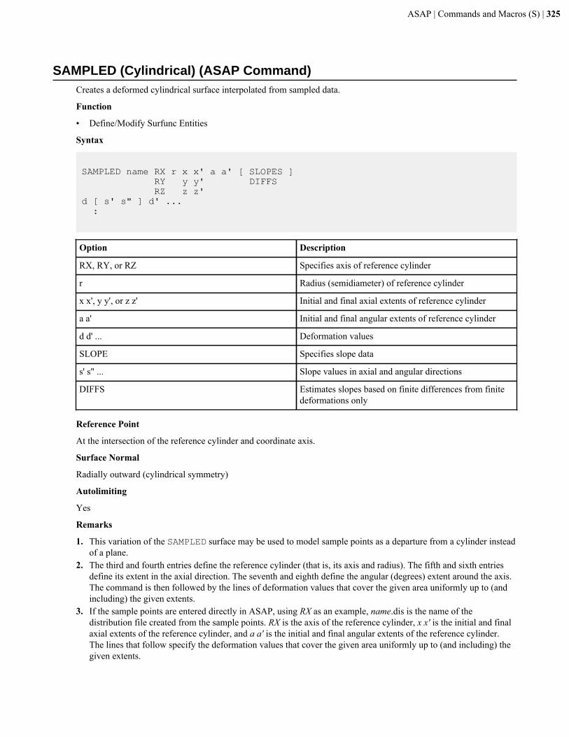
ASAP | Commands and Macros (S) | 325
SAMPLED (Cylindrical) (ASAP Command)Creates a deformed cylindrical surface interpolated from sampled data.
Function
• Define/Modify Surfunc Entities
Syntax
SAMPLED name RX r x x' a a' [ SLOPES ] RY y y' DIFFS RZ z z'd [ s' s" ] d' ... :
Option Description
RX, RY, or RZ Specifies axis of reference cylinder
r Radius (semidiameter) of reference cylinder
x x', y y', or z z' Initial and final axial extents of reference cylinder
a a' Initial and final angular extents of reference cylinder
d d' ... Deformation values
SLOPE Specifies slope data
s' s" ... Slope values in axial and angular directions
DIFFS Estimates slopes based on finite differences from finitedeformations only
Reference Point
At the intersection of the reference cylinder and coordinate axis.
Surface Normal
Radially outward (cylindrical symmetry)
Autolimiting
Yes
Remarks
1. This variation of the SAMPLED surface may be used to model sample points as a departure from a cylinder insteadof a plane.
2. The third and fourth entries define the reference cylinder (that is, its axis and radius). The fifth and sixth entriesdefine its extent in the axial direction. The seventh and eighth define the angular (degrees) extent around the axis.The command is then followed by the lines of deformation values that cover the given area uniformly up to (andincluding) the given extents.
3. If the sample points are entered directly in ASAP, using RX as an example, name.dis is the name of thedistribution file created from the sample points. RX is the axis of the reference cylinder, x x' is the initial and finalaxial extents of the reference cylinder, and a a' is the initial and final angular extents of the reference cylinder.The lines that follow specify the deformation values that cover the given area uniformly up to (and including) thegiven extents.
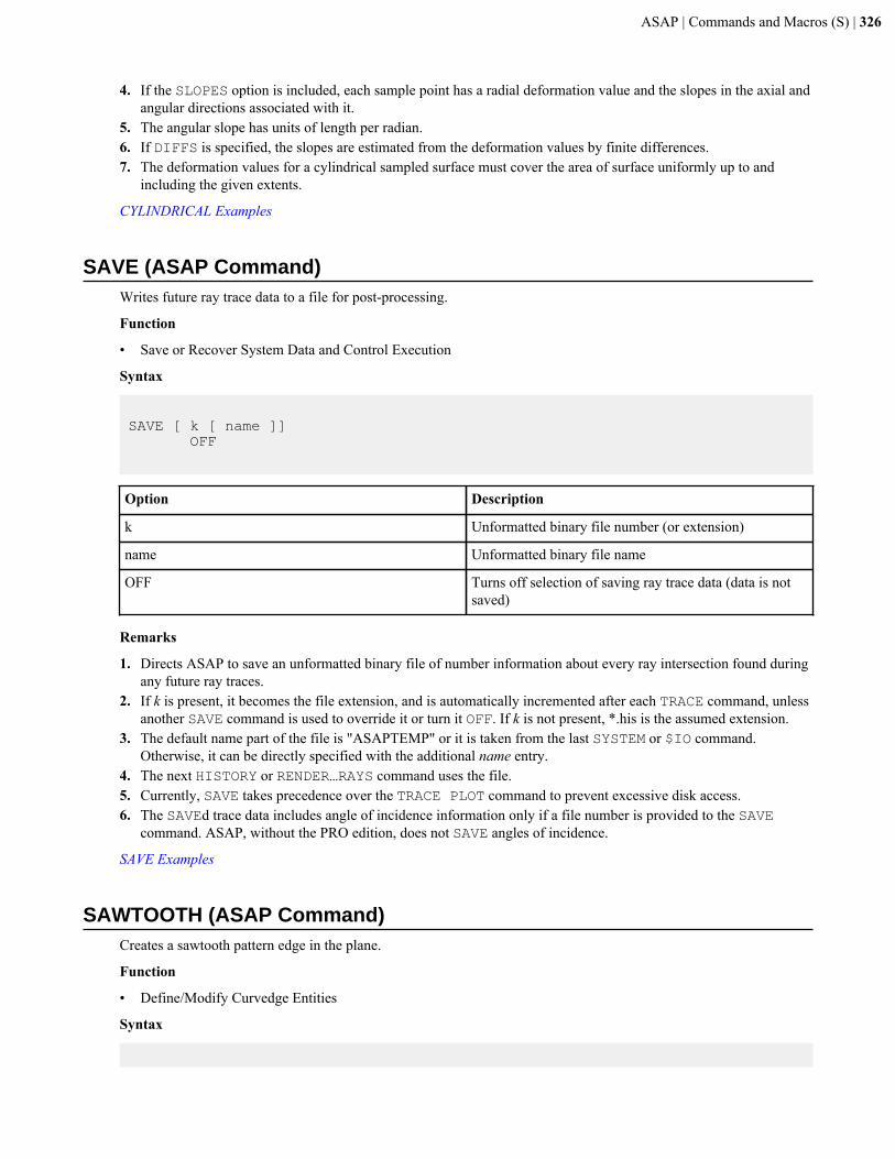
ASAP | Commands and Macros (S) | 326
4. If the SLOPES option is included, each sample point has a radial deformation value and the slopes in the axial andangular directions associated with it.
5. The angular slope has units of length per radian.6. If DIFFS is specified, the slopes are estimated from the deformation values by finite differences.7. The deformation values for a cylindrical sampled surface must cover the area of surface uniformly up to and
including the given extents.
CYLINDRICAL Examples
SAVE (ASAP Command)Writes future ray trace data to a file for post-processing.
Function
• Save or Recover System Data and Control Execution
Syntax
SAVE [ k [ name ]] OFF
Option Description
k Unformatted binary file number (or extension)
name Unformatted binary file name
OFF Turns off selection of saving ray trace data (data is notsaved)
Remarks
1. Directs ASAP to save an unformatted binary file of number information about every ray intersection found duringany future ray traces.
2. If k is present, it becomes the file extension, and is automatically incremented after each TRACE command, unlessanother SAVE command is used to override it or turn it OFF. If k is not present, *.his is the assumed extension.
3. The default name part of the file is "ASAPTEMP" or it is taken from the last SYSTEM or $IO command.Otherwise, it can be directly specified with the additional name entry.
4. The next HISTORY or RENDER…RAYS command uses the file.5. Currently, SAVE takes precedence over the TRACE PLOT command to prevent excessive disk access.6. The SAVEd trace data includes angle of incidence information only if a file number is provided to the SAVE
command. ASAP, without the PRO edition, does not SAVE angles of incidence.
SAVE Examples
SAWTOOTH (ASAP Command)Creates a sawtooth pattern edge in the plane.
Function
• Define/Modify Curvedge Entities
Syntax
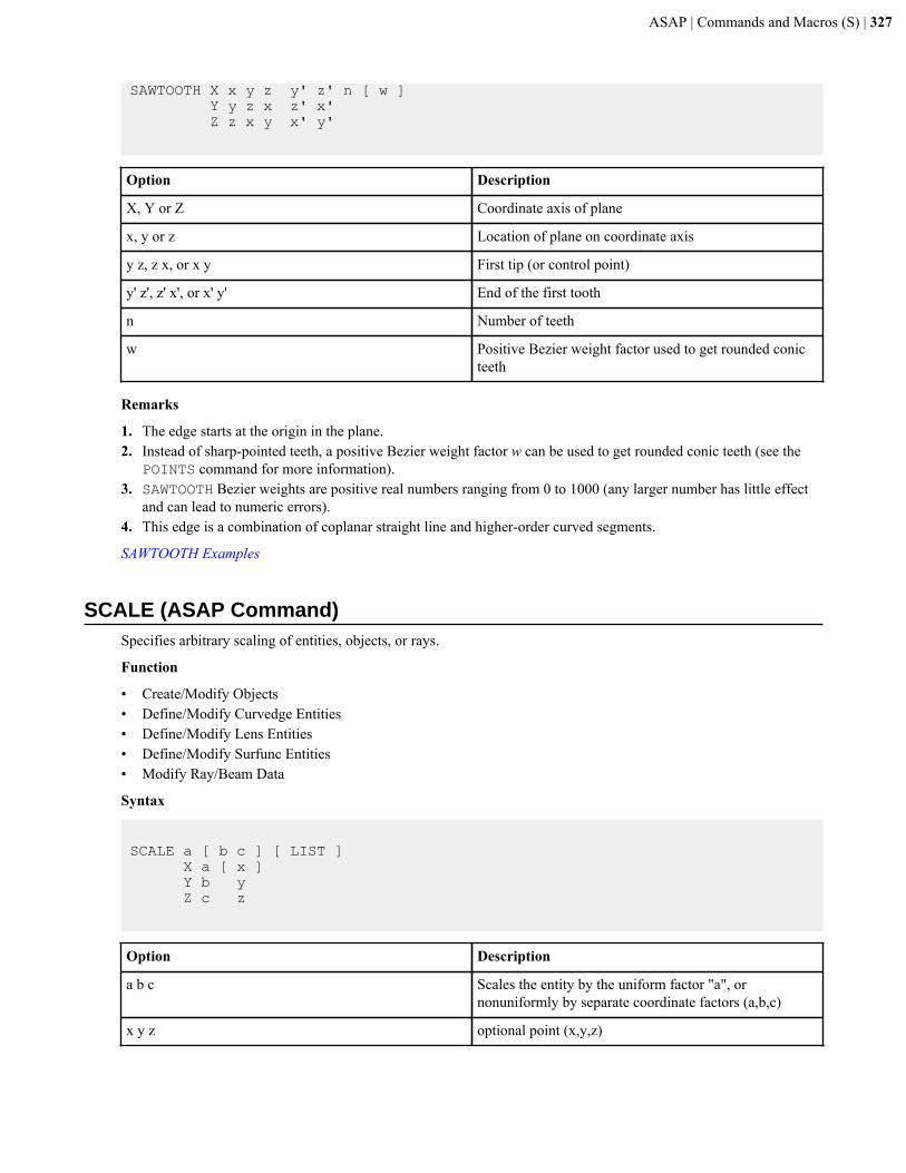
ASAP | Commands and Macros (S) | 327
SAWTOOTH X x y z y' z' n [ w ] Y y z x z' x' Z z x y x' y'
Option Description
X, Y or Z Coordinate axis of plane
x, y or z Location of plane on coordinate axis
y z, z x, or x y First tip (or control point)
y' z', z' x', or x' y' End of the first tooth
n Number of teeth
w Positive Bezier weight factor used to get rounded conicteeth
Remarks
1. The edge starts at the origin in the plane.2. Instead of sharp-pointed teeth, a positive Bezier weight factor w can be used to get rounded conic teeth (see the
POINTS command for more information).3. SAWTOOTH Bezier weights are positive real numbers ranging from 0 to 1000 (any larger number has little effect
and can lead to numeric errors).4. This edge is a combination of coplanar straight line and higher-order curved segments.
SAWTOOTH Examples
SCALE (ASAP Command)Specifies arbitrary scaling of entities, objects, or rays.
Function
• Create/Modify Objects• Define/Modify Curvedge Entities• Define/Modify Lens Entities• Define/Modify Surfunc Entities• Modify Ray/Beam Data
Syntax
SCALE a [ b c ] [ LIST ] X a [ x ] Y b y Z c z
Option Description
a b c Scales the entity by the uniform factor "a", ornonuniformly by separate coordinate factors (a,b,c)
x y z optional point (x,y,z)

ASAP | Commands and Macros (S) | 328
Option Description
LIST decodes transformation matrix into simple operations (ifpossible) and prints
Remarks
1. Uniformly scales the entity or object by the uniform factor a, or non-uniformly by separate factors (a,b,c), aboutthe optional point (x,y,z), which by default is the reference point to the entity or object.
2. ASAP scales relative to the original centroid as the reference point. Simple statistical noise can therefore createlarge variations in x, y, z positioning. When scaling sources that are centered about 0, 0, 0, it is best to specify x, y,z as 0, 0, 0 to fix their position.
3. The default for (a,b,c) is 1 (no scaling).4. When scaling rays anamorphically (unequal scaling in one or more directions), the angular direction cosines of
each ray are inversely scaled. An isotropic or Lambertian source does not remain isotropic or Lambertian afteranamorphic scaling.
5. Group SCALE with these commands: MATRIX; ROTATE; SHIFT; SKEW; PLACE; ALIGN; XEQ.
CAUTION
Do not use a nonuniform SCALE command to resize ray sets that were created using; for example, EMITTINGDATA. If you do, the angular distribution of the ray set is altered (see above).
Note: BRO recommends using the NORMALIZE command to rescale the axes of the distribution data filebefore creating rays.
SCALE Examples
SCALE FROM (ASAP Command)Scales from the given length units to the current system UNITS.
Function
• Modify Ray/Beam Data
Syntax
SCALE FROM units [ LIST ]
Option Description
units Given length units
LIST Decodes transformation matrix into simple operations (ifpossible) and prints
Remarks
1. Scales from the given length units to the current system UNITS.2. For allowable units strings, See the UNITS command.3. If system UNITS are not set, they are set to units and no scaling takes place.4. Automatically added to all imported CAD files to ensure that the geometry of the CAD file is in the proper system
units.
SCALE Examples
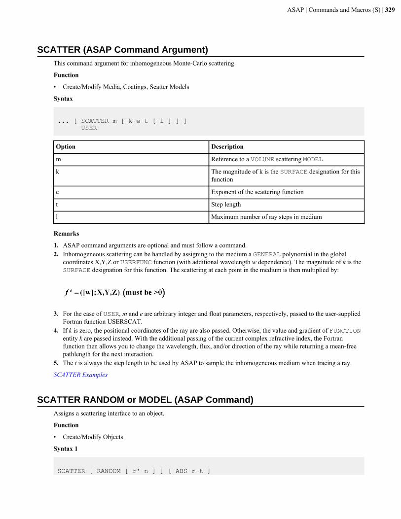
ASAP | Commands and Macros (S) | 329
SCATTER (ASAP Command Argument)This command argument for inhomogeneous Monte-Carlo scattering.
Function
• Create/Modify Media, Coatings, Scatter Models
Syntax
... [ SCATTER m [ k e t [ l ] ] ] USER
Option Description
m Reference to a VOLUME scattering MODEL
k The magnitude of k is the SURFACE designation for thisfunction
e Exponent of the scattering function
t Step length
l Maximum number of ray steps in medium
Remarks
1. ASAP command arguments are optional and must follow a command.2. Inhomogeneous scattering can be handled by assigning to the medium a GENERAL polynomial in the global
coordinates X,Y,Z or USERFUNC function (with additional wavelength w dependence). The magnitude of k is theSURFACE designation for this function. The scattering at each point in the medium is then multiplied by:
3. For the case of USER, m and e are arbitrary integer and float parameters, respectively, passed to the user-supplied
Fortran function USERSCAT.4. If k is zero, the positional coordinates of the ray are also passed. Otherwise, the value and gradient of FUNCTION
entity k are passed instead. With the additional passing of the current complex refractive index, the Fortranfunction then allows you to change the wavelength, flux, and/or direction of the ray while returning a mean-freepathlength for the next interaction.
5. The t is always the step length to be used by ASAP to sample the inhomogeneous medium when tracing a ray.
SCATTER Examples
SCATTER RANDOM or MODEL (ASAP Command)Assigns a scattering interface to an object.
Function
• Create/Modify Objects
Syntax 1
SCATTER [ RANDOM [ r' n ] ] [ ABS r t ]
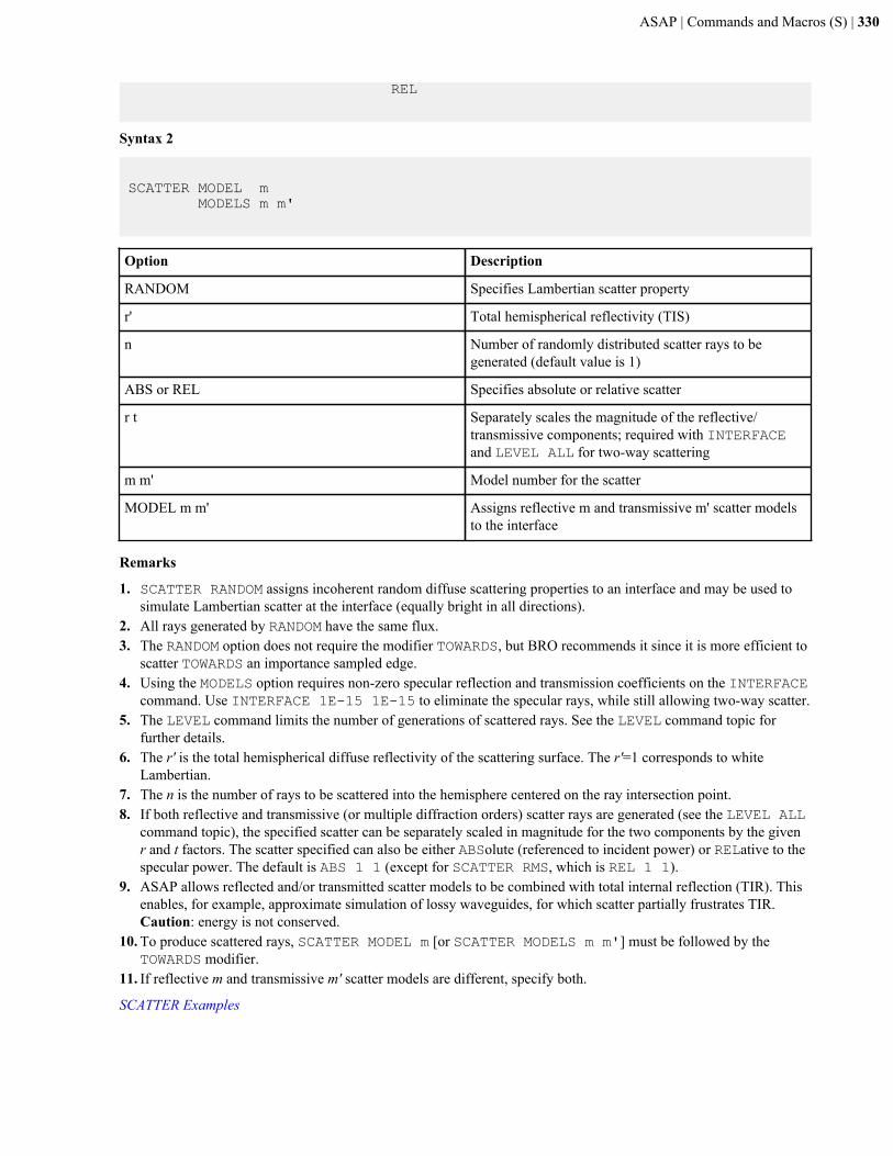
ASAP | Commands and Macros (S) | 330
REL
Syntax 2
SCATTER MODEL m MODELS m m'
Option Description
RANDOM Specifies Lambertian scatter property
r' Total hemispherical reflectivity (TIS)
n Number of randomly distributed scatter rays to begenerated (default value is 1)
ABS or REL Specifies absolute or relative scatter
r t Separately scales the magnitude of the reflective/transmissive components; required with INTERFACEand LEVEL ALL for two-way scattering
m m' Model number for the scatter
MODEL m m' Assigns reflective m and transmissive m' scatter modelsto the interface
Remarks
1. SCATTER RANDOM assigns incoherent random diffuse scattering properties to an interface and may be used tosimulate Lambertian scatter at the interface (equally bright in all directions).
2. All rays generated by RANDOM have the same flux.3. The RANDOM option does not require the modifier TOWARDS, but BRO recommends it since it is more efficient to
scatter TOWARDS an importance sampled edge.4. Using the MODELS option requires non-zero specular reflection and transmission coefficients on the INTERFACE
command. Use INTERFACE 1E-15 1E-15 to eliminate the specular rays, while still allowing two-way scatter.5. The LEVEL command limits the number of generations of scattered rays. See the LEVEL command topic for
further details.6. The r' is the total hemispherical diffuse reflectivity of the scattering surface. The r'=1 corresponds to white
Lambertian.7. The n is the number of rays to be scattered into the hemisphere centered on the ray intersection point.8. If both reflective and transmissive (or multiple diffraction orders) scatter rays are generated (see the LEVEL ALL
command topic), the specified scatter can be separately scaled in magnitude for the two components by the givenr and t factors. The scatter specified can also be either ABSolute (referenced to incident power) or RELative to thespecular power. The default is ABS 1 1 (except for SCATTER RMS, which is REL 1 1).
9. ASAP allows reflected and/or transmitted scatter models to be combined with total internal reflection (TIR). Thisenables, for example, approximate simulation of lossy waveguides, for which scatter partially frustrates TIR.Caution: energy is not conserved.
10. To produce scattered rays, SCATTER MODEL m [or SCATTER MODELS m m'] must be followed by theTOWARDS modifier.
11. If reflective m and transmissive m' scatter models are different, specify both.
SCATTER Examples
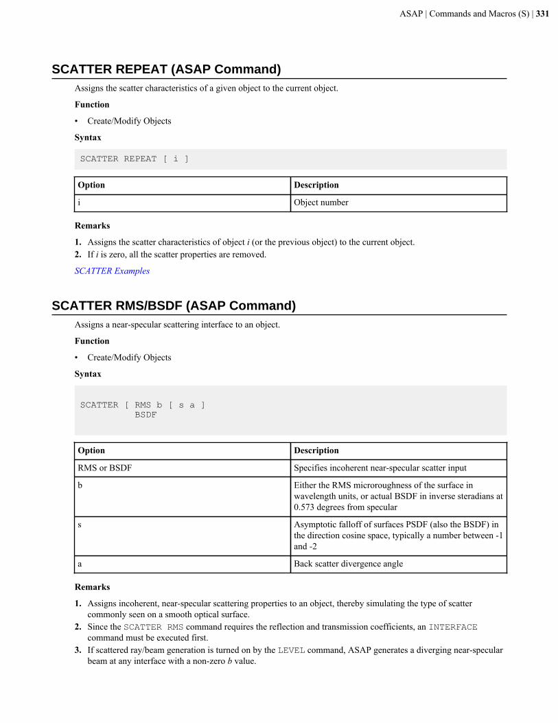
ASAP | Commands and Macros (S) | 331
SCATTER REPEAT (ASAP Command)Assigns the scatter characteristics of a given object to the current object.
Function
• Create/Modify Objects
Syntax
SCATTER REPEAT [ i ]
Option Description
i Object number
Remarks
1. Assigns the scatter characteristics of object i (or the previous object) to the current object.2. If i is zero, all the scatter properties are removed.
SCATTER Examples
SCATTER RMS/BSDF (ASAP Command)Assigns a near-specular scattering interface to an object.
Function
• Create/Modify Objects
Syntax
SCATTER [ RMS b [ s a ] BSDF
Option Description
RMS or BSDF Specifies incoherent near-specular scatter input
b Either the RMS microroughness of the surface inwavelength units, or actual BSDF in inverse steradians at0.573 degrees from specular
s Asymptotic falloff of surfaces PSDF (also the BSDF) inthe direction cosine space, typically a number between -1and -2
a Back scatter divergence angle
Remarks
1. Assigns incoherent, near-specular scattering properties to an object, thereby simulating the type of scattercommonly seen on a smooth optical surface.
2. Since the SCATTER RMS command requires the reflection and transmission coefficients, an INTERFACEcommand must be executed first.
3. If scattered ray/beam generation is turned on by the LEVEL command, ASAP generates a diverging near-specularbeam at any interface with a non-zero b value.
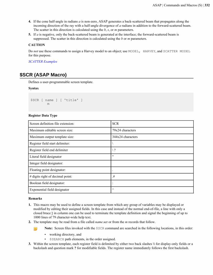
ASAP | Commands and Macros (S) | 332
4. If the cone half-angle in radians a is non-zero, ASAP generates a back-scattered beam that propagates along theincoming direction of the ray with a half-angle divergence of a radians in addition to the forward-scattered beam.The scatter in this direction is calculated using the b, s, or m parameters.
5. If a is negative, only the back-scattered beam is generated at the interface; the forward-scattered beam issuppressed. The scatter in this direction is calculated using the b or m parameters.
CAUTION
Do not use these commands to assign a Harvey model to an object; use MODEL, HARVEY, and SCATTER MODELfor this purpose.
SCATTER Examples
$SCR (ASAP Macro)Defines a user-programmable screen template.
Syntax
$SCR [ name ] [ 'title' ] m
Register Data Type
Screen definition file extension: SCR
Maximum editable screen size: 79x24 characters
Maximum output template size: 344x24 characters
Register field start delimiter: \
Register field end delimiter \ ?
Literal field designator "
Integer field designator:
Floating point designator: .
# digits right of decimal point: .#
Boolean field designator: :
Exponential field designator ^
Remarks
1. This macro may be used to define a screen template from which any group of variables may be displayed ormodified by editing their assigned fields. In this case and instead of the normal end-of-file, a line with only aclosed brace } in column one can be used to terminate the template definition and signal the beginning of up to1000 lines of 79 character-wide help text.
2. The template may be read from a file called name.scr or from the m records that follow.
Note: Screen files invoked with the $SCR command are searched in the following locations, in this order:
• working directory, and• $SEARCH path elements, in the order assigned.
3. Within the screen template, each register field is delimited by either two back slashes \\ for display-only fields or abackslash and question mark ? for modifiable fields. The register name immediately follows the first backslash.
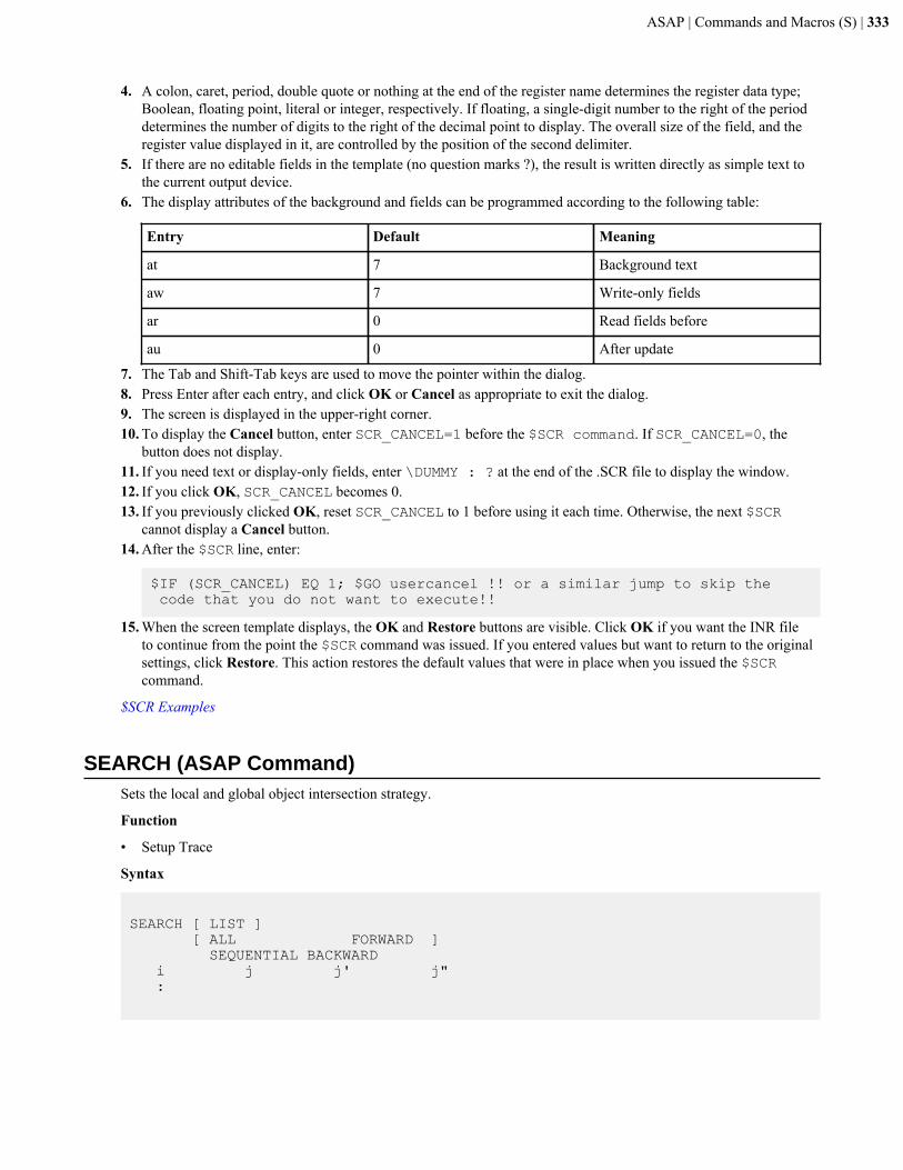
ASAP | Commands and Macros (S) | 333
4. A colon, caret, period, double quote or nothing at the end of the register name determines the register data type;Boolean, floating point, literal or integer, respectively. If floating, a single-digit number to the right of the perioddetermines the number of digits to the right of the decimal point to display. The overall size of the field, and theregister value displayed in it, are controlled by the position of the second delimiter.
5. If there are no editable fields in the template (no question marks ?), the result is written directly as simple text tothe current output device.
6. The display attributes of the background and fields can be programmed according to the following table:
Entry Default Meaning
at 7 Background text
aw 7 Write-only fields
ar 0 Read fields before
au 0 After update
7. The Tab and Shift-Tab keys are used to move the pointer within the dialog.8. Press Enter after each entry, and click OK or Cancel as appropriate to exit the dialog.9. The screen is displayed in the upper-right corner.10. To display the Cancel button, enter SCR_CANCEL=1 before the $SCR command. If SCR_CANCEL=0, the
button does not display.11. If you need text or display-only fields, enter \DUMMY : ? at the end of the .SCR file to display the window.12. If you click OK, SCR_CANCEL becomes 0.13. If you previously clicked OK, reset SCR_CANCEL to 1 before using it each time. Otherwise, the next $SCR
cannot display a Cancel button.14. After the $SCR line, enter:
$IF (SCR_CANCEL) EQ 1; $GO usercancel !! or a similar jump to skip the code that you do not want to execute!!
15. When the screen template displays, the OK and Restore buttons are visible. Click OK if you want the INR fileto continue from the point the $SCR command was issued. If you entered values but want to return to the originalsettings, click Restore. This action restores the default values that were in place when you issued the $SCRcommand.
$SCR Examples
SEARCH (ASAP Command)Sets the local and global object intersection strategy.
Function
• Setup Trace
Syntax
SEARCH [ LIST ] [ ALL FORWARD ] SEQUENTIAL BACKWARD i j j' j" :
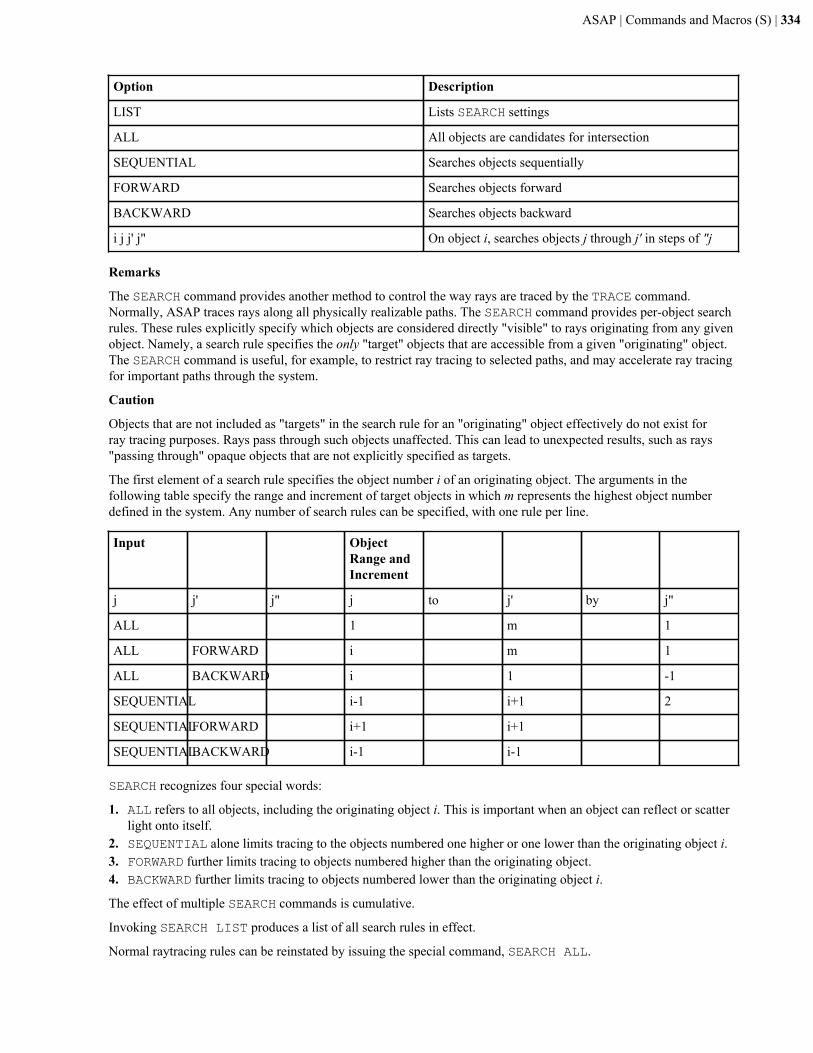
ASAP | Commands and Macros (S) | 334
Option Description
LIST Lists SEARCH settings
ALL All objects are candidates for intersection
SEQUENTIAL Searches objects sequentially
FORWARD Searches objects forward
BACKWARD Searches objects backward
i j j' j" On object i, searches objects j through j' in steps of "j
Remarks
The SEARCH command provides another method to control the way rays are traced by the TRACE command.Normally, ASAP traces rays along all physically realizable paths. The SEARCH command provides per-object searchrules. These rules explicitly specify which objects are considered directly "visible" to rays originating from any givenobject. Namely, a search rule specifies the only "target" objects that are accessible from a given "originating" object.The SEARCH command is useful, for example, to restrict ray tracing to selected paths, and may accelerate ray tracingfor important paths through the system.
Caution
Objects that are not included as "targets" in the search rule for an "originating" object effectively do not exist forray tracing purposes. Rays pass through such objects unaffected. This can lead to unexpected results, such as rays"passing through" opaque objects that are not explicitly specified as targets.
The first element of a search rule specifies the object number i of an originating object. The arguments in thefollowing table specify the range and increment of target objects in which m represents the highest object numberdefined in the system. Any number of search rules can be specified, with one rule per line.
Input ObjectRange andIncrement
j j' j" j to j' by j"
ALL 1 m 1
ALL FORWARD i m 1
ALL BACKWARD i 1 -1
SEQUENTIAL i-1 i+1 2
SEQUENTIALFORWARD i+1 i+1
SEQUENTIALBACKWARD i-1 i-1
SEARCH recognizes four special words:
1. ALL refers to all objects, including the originating object i. This is important when an object can reflect or scatterlight onto itself.
2. SEQUENTIAL alone limits tracing to the objects numbered one higher or one lower than the originating object i.3. FORWARD further limits tracing to objects numbered higher than the originating object.4. BACKWARD further limits tracing to objects numbered lower than the originating object i.
The effect of multiple SEARCH commands is cumulative.
Invoking SEARCH LIST produces a list of all search rules in effect.
Normal raytracing rules can be reinstated by issuing the special command, SEARCH ALL.
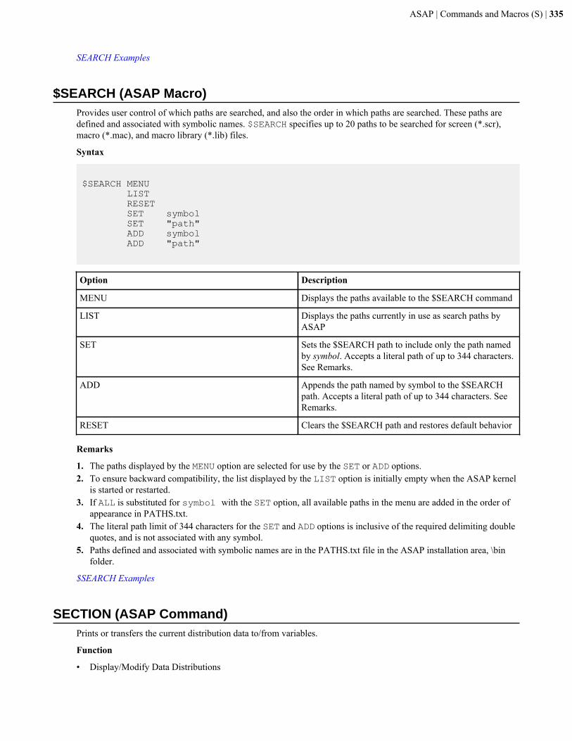
ASAP | Commands and Macros (S) | 335
SEARCH Examples
$SEARCH (ASAP Macro)Provides user control of which paths are searched, and also the order in which paths are searched. These paths aredefined and associated with symbolic names. $SEARCH specifies up to 20 paths to be searched for screen (*.scr),macro (*.mac), and macro library (*.lib) files.
Syntax
$SEARCH MENU LIST RESET SET symbol SET "path" ADD symbol ADD "path"
Option Description
MENU Displays the paths available to the $SEARCH command
LIST Displays the paths currently in use as search paths byASAP
SET Sets the $SEARCH path to include only the path namedby symbol. Accepts a literal path of up to 344 characters.See Remarks.
ADD Appends the path named by symbol to the $SEARCHpath. Accepts a literal path of up to 344 characters. SeeRemarks.
RESET Clears the $SEARCH path and restores default behavior
Remarks
1. The paths displayed by the MENU option are selected for use by the SET or ADD options.2. To ensure backward compatibility, the list displayed by the LIST option is initially empty when the ASAP kernel
is started or restarted.3. If ALL is substituted for symbol with the SET option, all available paths in the menu are added in the order of
appearance in PATHS.txt.4. The literal path limit of 344 characters for the SET and ADD options is inclusive of the required delimiting double
quotes, and is not associated with any symbol.5. Paths defined and associated with symbolic names are in the PATHS.txt file in the ASAP installation area, \bin
folder.
$SEARCH Examples
SECTION (ASAP Command)Prints or transfers the current distribution data to/from variables.
Function
• Display/Modify Data Distributions

ASAP | Commands and Macros (S) | 336
Syntax
SECTION [ m m' [ n n' ] ] [ GET ] PUT
Option Description
m m' n n' Range of pixels to be printed or transferred
GET Flag to transfer distribution data into variables
PUT Flag to put variables into distribution data
Remarks
1. Prints a table of current distribution data or transfers the current distribution data to or from an array of variables.
Print, GET into registers or PUT from registers the section of data:
f(i,j): i=m to m', j=n to n'2. If the GET or PUT options are used, the first data value is associated with register A0.3. If m'-m > 8 and n'-n > 24, the maximum allowable intrinsic register section is transferred:
SECTION (ASAP Command)
SEED (ASAP Command)Initializes the seed for the random number generator.
Function
• Setup Trace
Syntax
SEED [ n ] [ QUASI ] OFF
Option Description
n Seed number (default =2000000001)
QUASI Use a quasi random number sequence
OFF Cease using a quasi random number sequence
Remarks
1. Initializes the seed value for the random number generator used by the ROUGHNESS RANDOM, GRIDRANDOM, SCATTER RANDOM/TOWARDS and EMITTING commands.
2. For EMITTING sources, a QUASI random number Halton sequence can be used instead. In this case, only theremainder of n divided by 50 is used to select among 50 possible sequences.
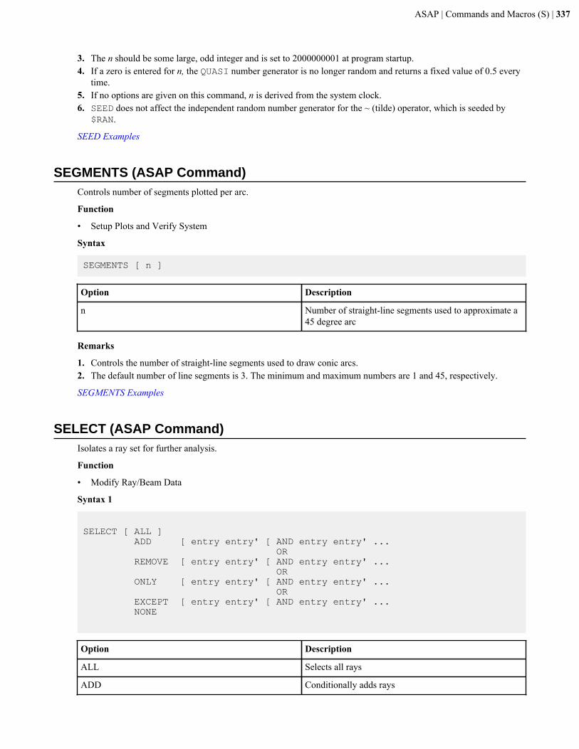
ASAP | Commands and Macros (S) | 337
3. The n should be some large, odd integer and is set to 2000000001 at program startup.4. If a zero is entered for n, the QUASI number generator is no longer random and returns a fixed value of 0.5 every
time.5. If no options are given on this command, n is derived from the system clock.6. SEED does not affect the independent random number generator for the ~ (tilde) operator, which is seeded by
$RAN.
SEED Examples
SEGMENTS (ASAP Command)Controls number of segments plotted per arc.
Function
• Setup Plots and Verify System
Syntax
SEGMENTS [ n ]
Option Description
n Number of straight-line segments used to approximate a45 degree arc
Remarks
1. Controls the number of straight-line segments used to draw conic arcs.2. The default number of line segments is 3. The minimum and maximum numbers are 1 and 45, respectively.
SEGMENTS Examples
SELECT (ASAP Command)Isolates a ray set for further analysis.
Function
• Modify Ray/Beam Data
Syntax 1
SELECT [ ALL ] ADD [ entry entry' [ AND entry entry' ... OR REMOVE [ entry entry' [ AND entry entry' ... OR ONLY [ entry entry' [ AND entry entry' ... OR EXCEPT [ entry entry' [ AND entry entry' ... NONE
Option Description
ALL Selects all rays
ADD Conditionally adds rays
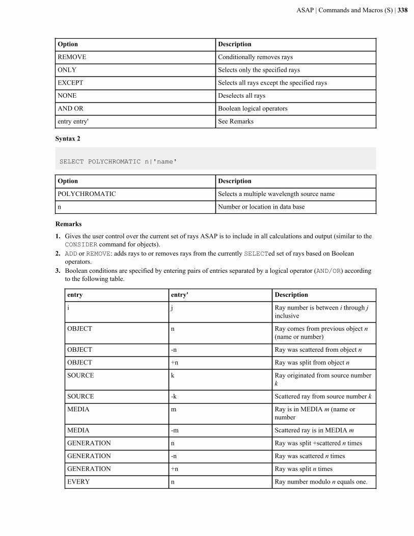
ASAP | Commands and Macros (S) | 338
Option Description
REMOVE Conditionally removes rays
ONLY Selects only the specified rays
EXCEPT Selects all rays except the specified rays
NONE Deselects all rays
AND OR Boolean logical operators
entry entry' See Remarks
Syntax 2
SELECT POLYCHROMATIC n|'name'
Option Description
POLYCHROMATIC Selects a multiple wavelength source name
n Number or location in data base
Remarks
1. Gives the user control over the current set of rays ASAP is to include in all calculations and output (similar to theCONSIDER command for objects).
2. ADD or REMOVE: adds rays to or removes rays from the currently SELECTed set of rays based on Booleanoperators.
3. Boolean conditions are specified by entering pairs of entries separated by a logical operator (AND/OR) accordingto the following table.
entry entry' Description
i j Ray number is between i through jinclusive
OBJECT n Ray comes from previous object n(name or number)
OBJECT -n Ray was scattered from object n
OBJECT +n Ray was split from object n
SOURCE k Ray originated from source numberk
SOURCE -k Scattered ray from source number k
MEDIA m Ray is in MEDIA m (name ornumber
MEDIA -m Scattered ray is in MEDIA m
GENERATION n Ray was split +scattered n times
GENERATION -n Ray was scattered n times
GENERATION +n Ray was split n times
EVERY n Ray number modulo n equals one.
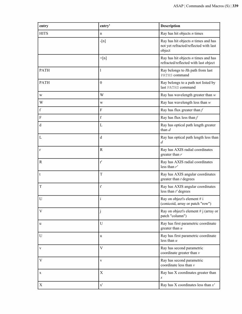
ASAP | Commands and Macros (S) | 339
entry entry' Description
HITS n Ray has hit objects n times
-[n] Ray has hit objects n times and hasnot yet refracted/reflected with lastobject
+[n] Ray has hit objects n times and hasrefracted/reflected with last object
PATH l Ray belongs to lth path from lastPATHS command
PATH 0 Ray belongs to a path not listed bylast PATHS command
w W Ray has wavelength greater than w
W w Ray has wavelength less than w
f F Ray has flux greater than f
F f Ray has flux less than f
d L Ray has optical path length greaterthan d
L d Ray has optical path length less thand
r R Ray has AXIS radial coordinatesgreater than r
R r' Ray has AXIS radial coordinatesless than r'
t T Ray has AXIS angular coordinatesgreater than t degrees
T t' Ray has AXIS angular coordinatesless than t' degrees
U i Ray on object's element # i(conicoid, array or patch "row")
V j Ray on object's element # j (array orpatch "column")
u U Ray has first parametric coordinategreater than u
U u Ray has first parametric coordinateless than u
v V Ray has second parametriccoordinate greater than v
V v Ray has second parametriccoordinate less than v
x X Ray has X coordinates greater thanx
X x' Ray has X coordinates less than x'
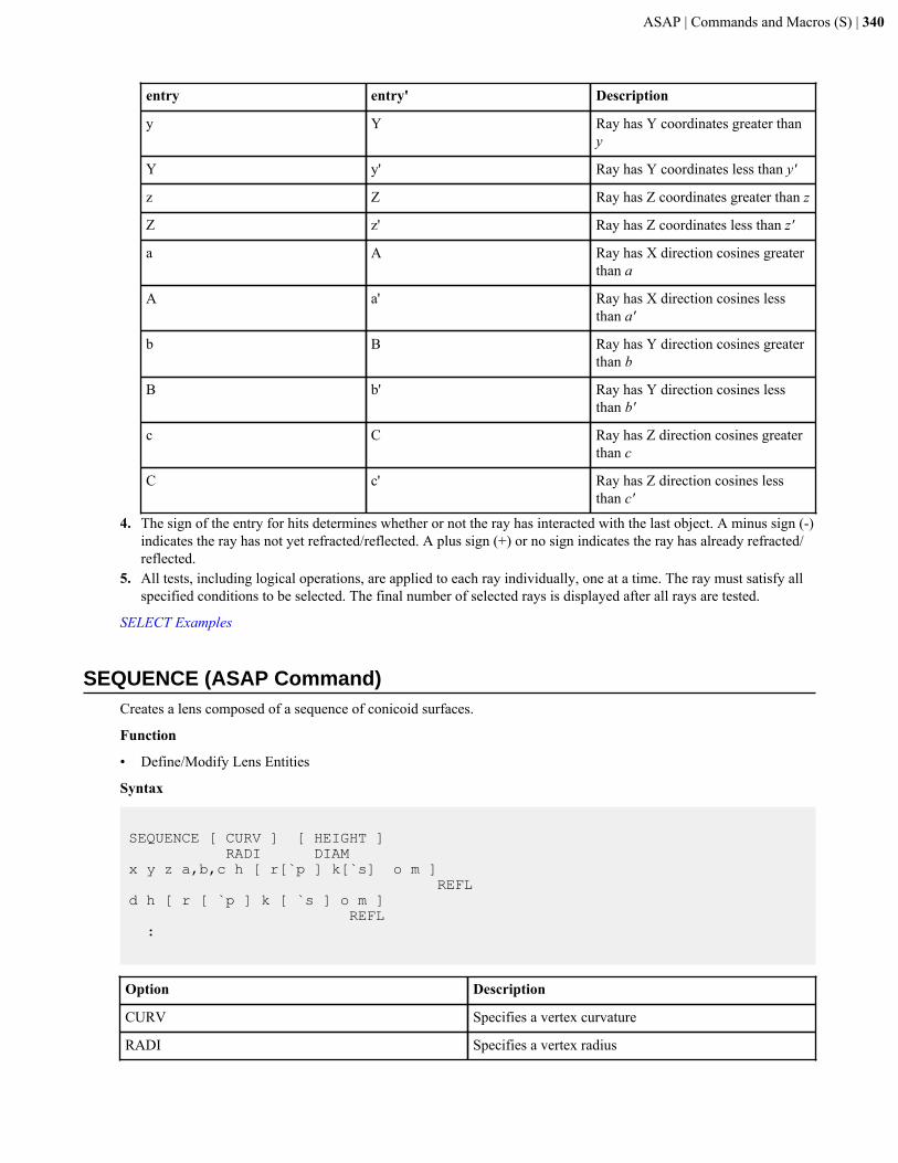
ASAP | Commands and Macros (S) | 340
entry entry' Description
y Y Ray has Y coordinates greater thany
Y y' Ray has Y coordinates less than y'
z Z Ray has Z coordinates greater than z
Z z' Ray has Z coordinates less than z'
a A Ray has X direction cosines greaterthan a
A a' Ray has X direction cosines lessthan a'
b B Ray has Y direction cosines greaterthan b
B b' Ray has Y direction cosines lessthan b'
c C Ray has Z direction cosines greaterthan c
C c' Ray has Z direction cosines lessthan c'
4. The sign of the entry for hits determines whether or not the ray has interacted with the last object. A minus sign (-)indicates the ray has not yet refracted/reflected. A plus sign (+) or no sign indicates the ray has already refracted/reflected.
5. All tests, including logical operations, are applied to each ray individually, one at a time. The ray must satisfy allspecified conditions to be selected. The final number of selected rays is displayed after all rays are tested.
SELECT Examples
SEQUENCE (ASAP Command)Creates a lens composed of a sequence of conicoid surfaces.
Function
• Define/Modify Lens Entities
Syntax
SEQUENCE [ CURV ] [ HEIGHT ] RADI DIAMx y z a,b,c h [ r[`p ] k[`s] o m ] REFLd h [ r [ `p ] k [ `s ] o m ] REFL :
Option Description
CURV Specifies a vertex curvature
RADI Specifies a vertex radius
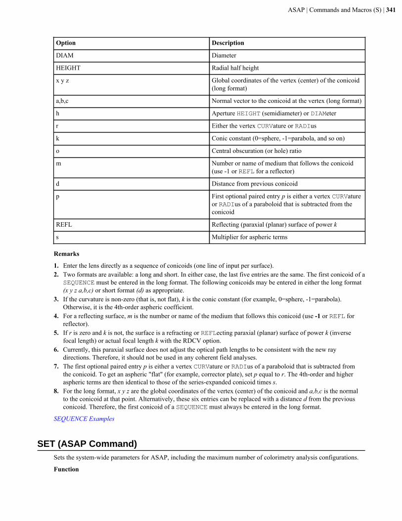
ASAP | Commands and Macros (S) | 341
Option Description
DIAM Diameter
HEIGHT Radial half height
x y z Global coordinates of the vertex (center) of the conicoid(long format)
a,b,c Normal vector to the conicoid at the vertex (long format)
h Aperture HEIGHT (semidiameter) or DIAMeter
r Either the vertex CURVature or RADIus
k Conic constant (0=sphere, -1=parabola, and so on)
o Central obscuration (or hole) ratio
m Number or name of medium that follows the conicoid(use -1 or REFL for a reflector)
d Distance from previous conicoid
p First optional paired entry p is either a vertex CURVatureor RADIus of a paraboloid that is subtracted from theconicoid
REFL Reflecting (paraxial (planar) surface of power k
s Multiplier for aspheric terms
Remarks
1. Enter the lens directly as a sequence of conicoids (one line of input per surface).2. Two formats are available: a long and short. In either case, the last five entries are the same. The first conicoid of a
SEQUENCE must be entered in the long format. The following conicoids may be entered in either the long format(x y z a,b,c) or short format (d) as appropriate.
3. If the curvature is non-zero (that is, not flat), k is the conic constant (for example, 0=sphere, -1=parabola).Otherwise, it is the 4th-order aspheric coefficient.
4. For a reflecting surface, m is the number or name of the medium that follows this conicoid (use -1 or REFL forreflector).
5. If r is zero and k is not, the surface is a refracting or REFLecting paraxial (planar) surface of power k (inversefocal length) or actual focal length k with the RDCV option.
6. Currently, this paraxial surface does not adjust the optical path lengths to be consistent with the new raydirections. Therefore, it should not be used in any coherent field analyses.
7. The first optional paired entry p is either a vertex CURVature or RADIus of a paraboloid that is subtracted fromthe conicoid. To get an aspheric "flat" (for example, corrector plate), set p equal to r. The 4th-order and higheraspheric terms are then identical to those of the series-expanded conicoid times s.
8. For the long format, x y z are the global coordinates of the vertex (center) of the conicoid and a,b,c is the normalto the conicoid at that point. Alternatively, these six entries can be replaced with a distance d from the previousconicoid. Therefore, the first conicoid of a SEQUENCE must always be entered in the long format.
SEQUENCE Examples
SET (ASAP Command)Sets the system-wide parameters for ASAP, including the maximum number of colorimetry analysis configurations.
Function
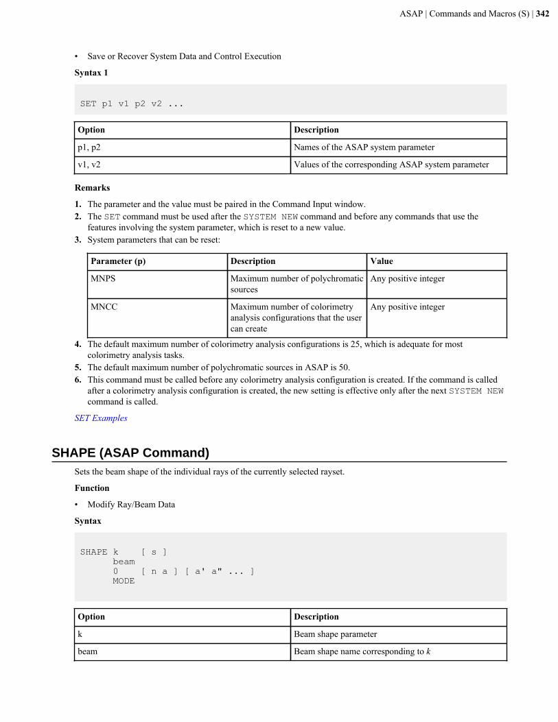
ASAP | Commands and Macros (S) | 342
• Save or Recover System Data and Control Execution
Syntax 1
SET p1 v1 p2 v2 ...
Option Description
p1, p2 Names of the ASAP system parameter
v1, v2 Values of the corresponding ASAP system parameter
Remarks
1. The parameter and the value must be paired in the Command Input window.2. The SET command must be used after the SYSTEM NEW command and before any commands that use the
features involving the system parameter, which is reset to a new value.3. System parameters that can be reset:
Parameter (p) Description Value
MNPS Maximum number of polychromaticsources
Any positive integer
MNCC Maximum number of colorimetryanalysis configurations that the usercan create
Any positive integer
4. The default maximum number of colorimetry analysis configurations is 25, which is adequate for mostcolorimetry analysis tasks.
5. The default maximum number of polychromatic sources in ASAP is 50.6. This command must be called before any colorimetry analysis configuration is created. If the command is called
after a colorimetry analysis configuration is created, the new setting is effective only after the next SYSTEM NEWcommand is called.
SET Examples
SHAPE (ASAP Command)Sets the beam shape of the individual rays of the currently selected rayset.
Function
• Modify Ray/Beam Data
Syntax
SHAPE k [ s ] beam 0 [ n a ] [ a' a" ... ] MODE
Option Description
k Beam shape parameter
beam Beam shape name corresponding to k
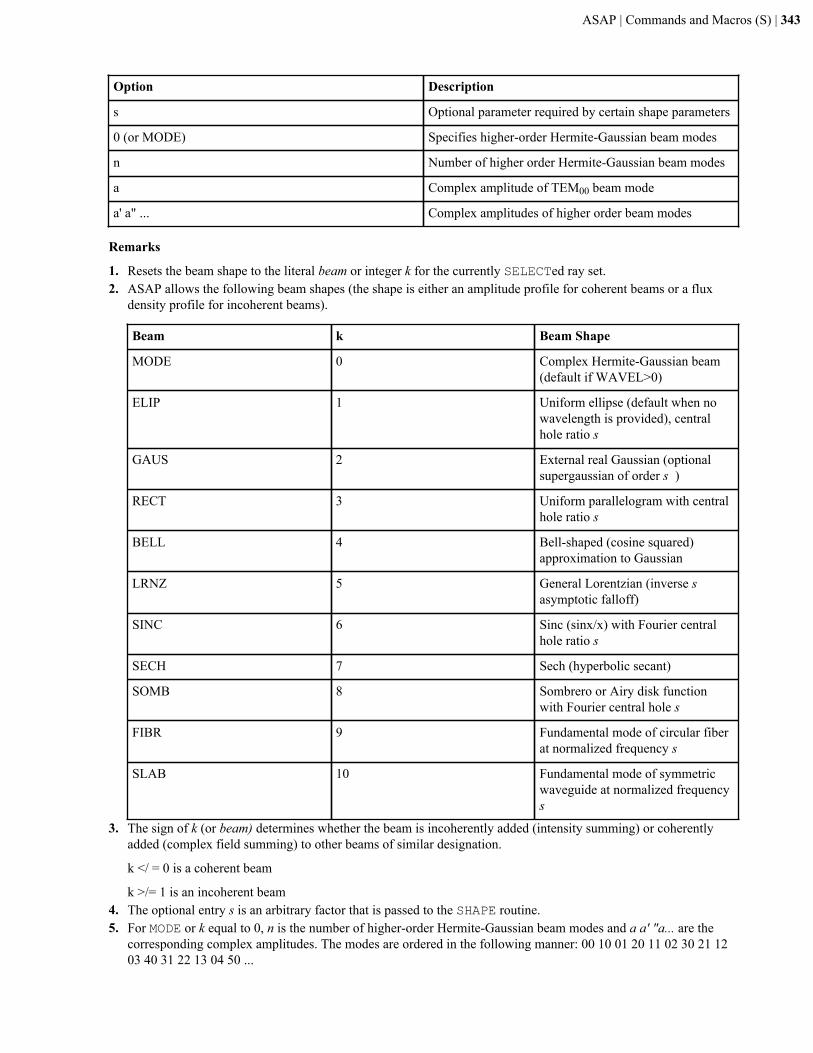
ASAP | Commands and Macros (S) | 343
Option Description
s Optional parameter required by certain shape parameters
0 (or MODE) Specifies higher-order Hermite-Gaussian beam modes
n Number of higher order Hermite-Gaussian beam modes
a Complex amplitude of TEM00 beam mode
a' a" ... Complex amplitudes of higher order beam modes
Remarks
1. Resets the beam shape to the literal beam or integer k for the currently SELECTed ray set.2. ASAP allows the following beam shapes (the shape is either an amplitude profile for coherent beams or a flux
density profile for incoherent beams).
Beam k Beam Shape
MODE 0 Complex Hermite-Gaussian beam(default if WAVEL>0)
ELIP 1 Uniform ellipse (default when nowavelength is provided), centralhole ratio s
GAUS 2 External real Gaussian (optionalsupergaussian of order s )
RECT 3 Uniform parallelogram with centralhole ratio s
BELL 4 Bell-shaped (cosine squared)approximation to Gaussian
LRNZ 5 General Lorentzian (inverse s asymptotic falloff)
SINC 6 Sinc (sinx/x) with Fourier centralhole ratio s
SECH 7 Sech (hyperbolic secant)
SOMB 8 Sombrero or Airy disk functionwith Fourier central hole s
FIBR 9 Fundamental mode of circular fiberat normalized frequency s
SLAB 10 Fundamental mode of symmetricwaveguide at normalized frequencys
3. The sign of k (or beam) determines whether the beam is incoherently added (intensity summing) or coherentlyadded (complex field summing) to other beams of similar designation.
k </ = 0 is a coherent beam
k >/= 1 is an incoherent beam4. The optional entry s is an arbitrary factor that is passed to the SHAPE routine.5. For MODE or k equal to 0, n is the number of higher-order Hermite-Gaussian beam modes and a a' "a... are the
corresponding complex amplitudes. The modes are ordered in the following manner: 00 10 01 20 11 02 30 21 1203 40 31 22 13 04 50 ...
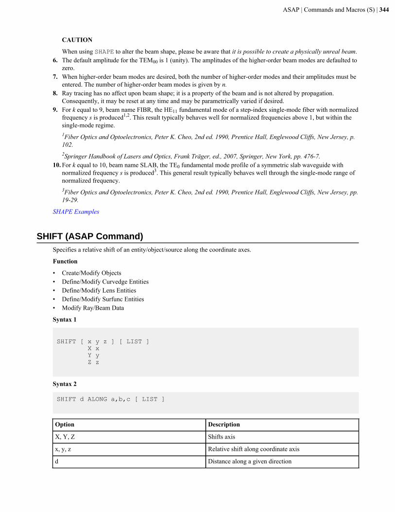
ASAP | Commands and Macros (S) | 344
CAUTION
When using SHAPE to alter the beam shape, please be aware that it is possible to create a physically unreal beam.6. The default amplitude for the TEM00 is 1 (unity). The amplitudes of the higher-order beam modes are defaulted to
zero.7. When higher-order beam modes are desired, both the number of higher-order modes and their amplitudes must be
entered. The number of higher-order beam modes is given by n.8. Ray tracing has no affect upon beam shape; it is a property of the beam and is not altered by propagation.
Consequently, it may be reset at any time and may be parametrically varied if desired.9. For k equal to 9, beam name FIBR, the HE11 fundamental mode of a step-index single-mode fiber with normalized
frequency s is produced1,2. This result typically behaves well for normalized frequencies above 1, but within thesingle-mode regime.1Fiber Optics and Optoelectronics, Peter K. Cheo, 2nd ed. 1990, Prentice Hall, Englewood Cliffs, New Jersey, p.102.2Springer Handbook of Lasers and Optics, Frank Träger, ed., 2007, Springer, New York, pp. 476-7.
10. For k equal to 10, beam name SLAB, the TE0 fundamental mode profile of a symmetric slab waveguide withnormalized frequency s is produced3. This general result typically behaves well through the single-mode range ofnormalized frequency.3Fiber Optics and Optoelectronics, Peter K. Cheo, 2nd ed. 1990, Prentice Hall, Englewood Cliffs, New Jersey, pp.19-29.
SHAPE Examples
SHIFT (ASAP Command)Specifies a relative shift of an entity/object/source along the coordinate axes.
Function
• Create/Modify Objects• Define/Modify Curvedge Entities• Define/Modify Lens Entities• Define/Modify Surfunc Entities• Modify Ray/Beam Data
Syntax 1
SHIFT [ x y z ] [ LIST ] X x Y y Z z
Syntax 2
SHIFT d ALONG a,b,c [ LIST ]
Option Description
X, Y, Z Shifts axis
x, y, z Relative shift along coordinate axis
d Distance along a given direction
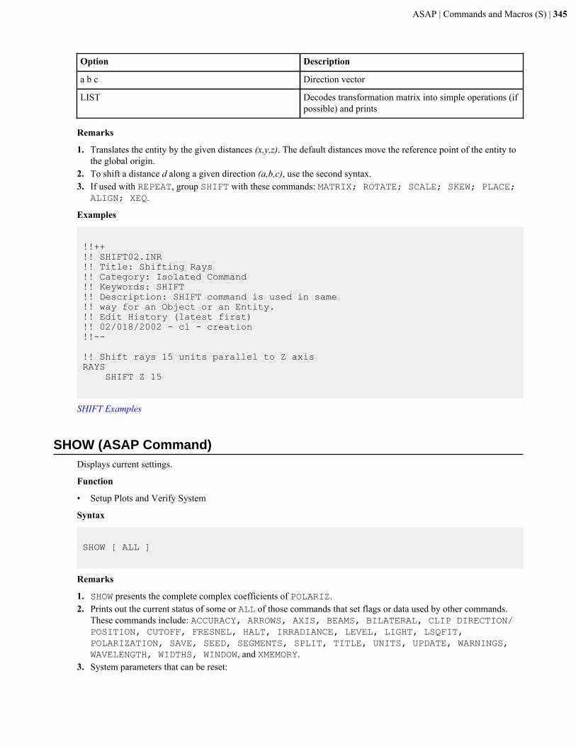
ASAP | Commands and Macros (S) | 345
Option Description
a b c Direction vector
LIST Decodes transformation matrix into simple operations (ifpossible) and prints
Remarks
1. Translates the entity by the given distances (x,y,z). The default distances move the reference point of the entity tothe global origin.
2. To shift a distance d along a given direction (a,b,c), use the second syntax.3. If used with REPEAT, group SHIFT with these commands: MATRIX; ROTATE; SCALE; SKEW; PLACE;
ALIGN; XEQ.
Examples
!!++!! SHIFT02.INR!! Title: Shifting Rays!! Category: Isolated Command!! Keywords: SHIFT !! Description: SHIFT command is used in same!! way for an Object or an Entity.!! Edit History (latest first)!! 02/018/2002 - cl - creation!!--
!! Shift rays 15 units parallel to Z axisRAYS SHIFT Z 15
SHIFT Examples
SHOW (ASAP Command)Displays current settings.
Function
• Setup Plots and Verify System
Syntax
SHOW [ ALL ]
Remarks
1. SHOW presents the complete complex coefficients of POLARIZ.2. Prints out the current status of some or ALL of those commands that set flags or data used by other commands.
These commands include: ACCURACY, ARROWS, AXIS, BEAMS, BILATERAL, CLIP DIRECTION/POSITION, CUTOFF, FRESNEL, HALT, IRRADIANCE, LEVEL, LIGHT, LSQFIT,POLARIZATION, SAVE, SEED, SEGMENTS, SPLIT, TITLE, UNITS, UPDATE, WARNINGS,WAVELENGTH, WIDTHS, WINDOW, and XMEMORY.
3. System parameters that can be reset:
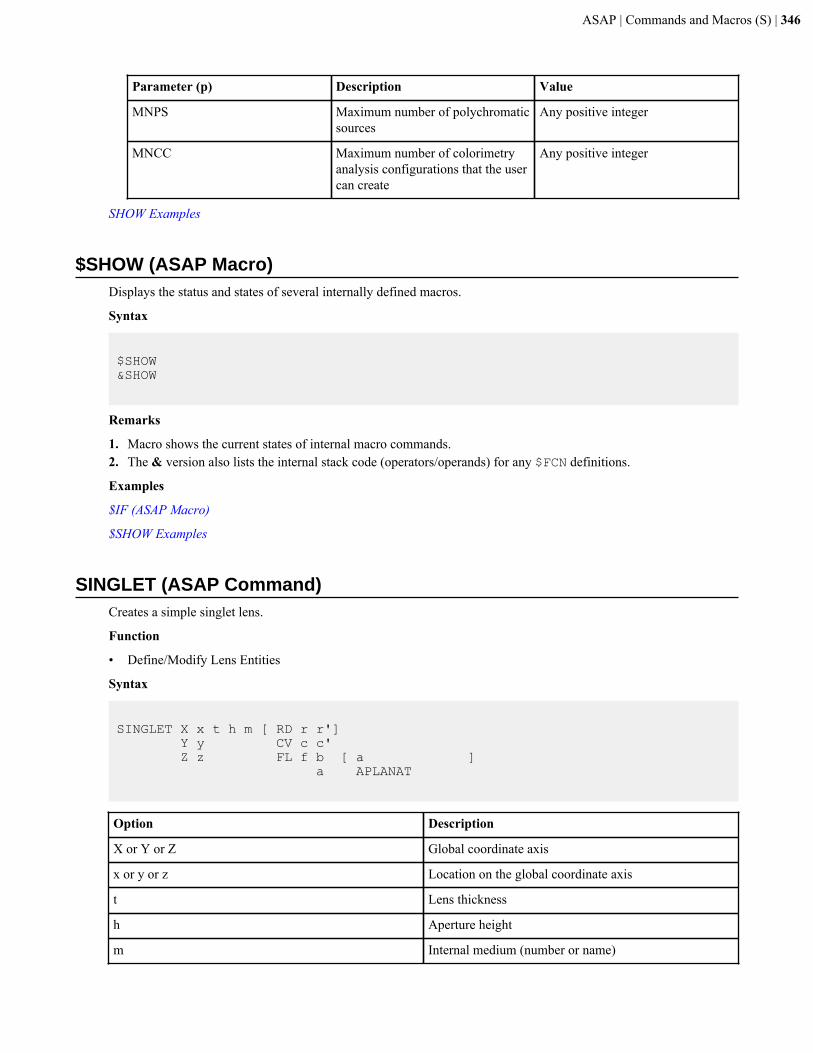
ASAP | Commands and Macros (S) | 346
Parameter (p) Description Value
MNPS Maximum number of polychromaticsources
Any positive integer
MNCC Maximum number of colorimetryanalysis configurations that the usercan create
Any positive integer
SHOW Examples
$SHOW (ASAP Macro)Displays the status and states of several internally defined macros.
Syntax
$SHOW&SHOW
Remarks
1. Macro shows the current states of internal macro commands.2. The & version also lists the internal stack code (operators/operands) for any $FCN definitions.
Examples
$IF (ASAP Macro)
$SHOW Examples
SINGLET (ASAP Command)Creates a simple singlet lens.
Function
• Define/Modify Lens Entities
Syntax
SINGLET X x t h m [ RD r r'] Y y CV c c' Z z FL f b [ a ] a APLANAT
Option Description
X or Y or Z Global coordinate axis
x or y or z Location on the global coordinate axis
t Lens thickness
h Aperture height
m Internal medium (number or name)
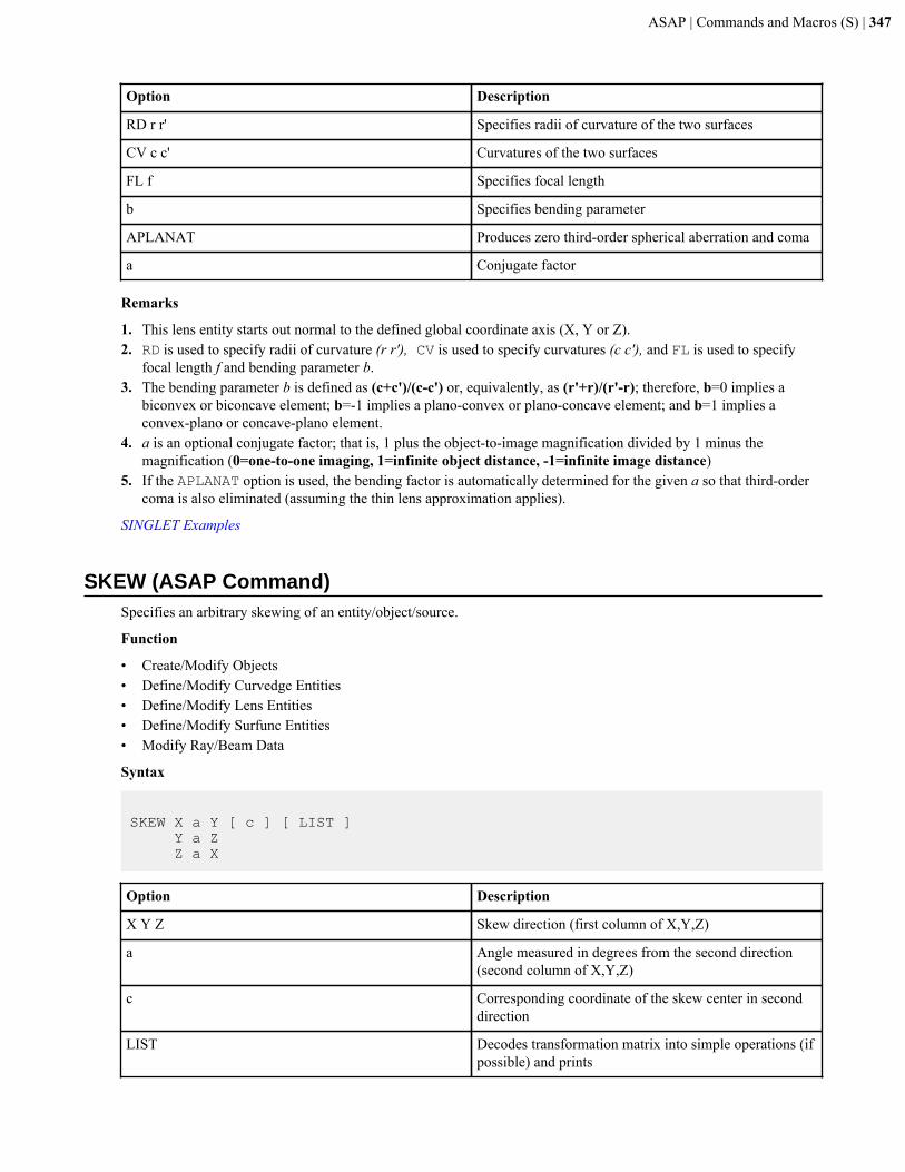
ASAP | Commands and Macros (S) | 347
Option Description
RD r r' Specifies radii of curvature of the two surfaces
CV c c' Curvatures of the two surfaces
FL f Specifies focal length
b Specifies bending parameter
APLANAT Produces zero third-order spherical aberration and coma
a Conjugate factor
Remarks
1. This lens entity starts out normal to the defined global coordinate axis (X, Y or Z).2. RD is used to specify radii of curvature (r r'), CV is used to specify curvatures (c c'), and FL is used to specify
focal length f and bending parameter b.3. The bending parameter b is defined as (c+c')/(c-c') or, equivalently, as (r'+r)/(r'-r); therefore, b=0 implies a
biconvex or biconcave element; b=-1 implies a plano-convex or plano-concave element; and b=1 implies aconvex-plano or concave-plano element.
4. a is an optional conjugate factor; that is, 1 plus the object-to-image magnification divided by 1 minus themagnification (0=one-to-one imaging, 1=infinite object distance, -1=infinite image distance)
5. If the APLANAT option is used, the bending factor is automatically determined for the given a so that third-ordercoma is also eliminated (assuming the thin lens approximation applies).
SINGLET Examples
SKEW (ASAP Command)Specifies an arbitrary skewing of an entity/object/source.
Function
• Create/Modify Objects• Define/Modify Curvedge Entities• Define/Modify Lens Entities• Define/Modify Surfunc Entities• Modify Ray/Beam Data
Syntax
SKEW X a Y [ c ] [ LIST ] Y a Z Z a X
Option Description
X Y Z Skew direction (first column of X,Y,Z)
a Angle measured in degrees from the second direction(second column of X,Y,Z)
c Corresponding coordinate of the skew center in seconddirection
LIST Decodes transformation matrix into simple operations (ifpossible) and prints
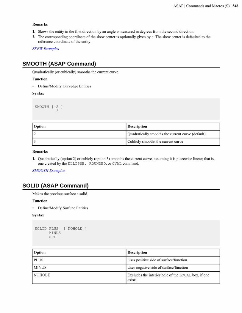
ASAP | Commands and Macros (S) | 348
Remarks
1. Skews the entity in the first direction by an angle a measured in degrees from the second direction.2. The corresponding coordinate of the skew center is optionally given by c. The skew center is defaulted to the
reference coordinate of the entity.
SKEW Examples
SMOOTH (ASAP Command)Quadratically (or cubically) smooths the current curve.
Function
• Define/Modify Curvedge Entities
Syntax
SMOOTH [ 2 ] 3
Option Description
2 Quadratically smooths the current curve (default)
3 Cublicly smooths the current curve
Remarks
1. Quadratically (option 2) or cubicly (option 3) smooths the current curve, assuming it is piecewise linear; that is,one created by the ELLIPSE, ROUNDED, or OVAL command.
SMOOTH Examples
SOLID (ASAP Command)Makes the previous surface a solid.
Function
• Define/Modify Surfunc Entities
Syntax
SOLID PLUS [ NOHOLE ] MINUS OFF
Option Description
PLUS Uses positive side of surface/function
MINUS Uses negative side of surface/function
NOHOLE Excludes the interior hole of the LOCAL box, if oneexists
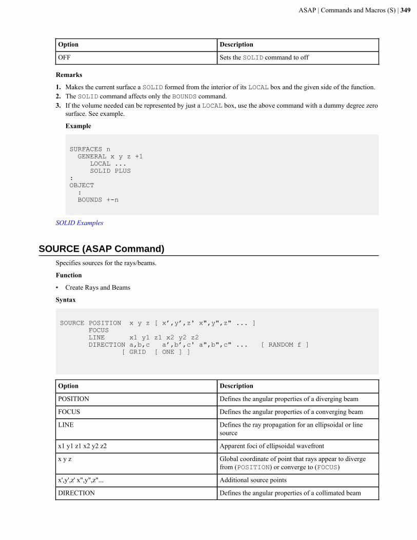
ASAP | Commands and Macros (S) | 349
Option Description
OFF Sets the SOLID command to off
Remarks
1. Makes the current surface a SOLID formed from the interior of its LOCAL box and the given side of the function.2. The SOLID command affects only the BOUNDS command.3. If the volume needed can be represented by just a LOCAL box, use the above command with a dummy degree zero
surface. See example.
Example
SURFACES n GENERAL x y z +1 LOCAL ... SOLID PLUS:OBJECT : BOUNDS +-n
SOLID Examples
SOURCE (ASAP Command)Specifies sources for the rays/beams.
Function
• Create Rays and Beams
Syntax
SOURCE POSITION x y z [ x’,y’,z' x",y",z" ... ] FOCUS LINE x1 y1 z1 x2 y2 z2 DIRECTION a,b,c a’,b’,c' a",b",c" ... [ RANDOM f ] [ GRID [ ONE ] ]
Option Description
POSITION Defines the angular properties of a diverging beam
FOCUS Defines the angular properties of a converging beam
LINE Defines the ray propagation for an ellipsoidal or linesource
x1 y1 z1 x2 y2 z2 Apparent foci of ellipsoidal wavefront
x y z Global coordinate of point that rays appear to divergefrom (POSITION) or converge to (FOCUS)
x',y',z' x",y",z"... Additional source points
DIRECTION Defines the angular properties of a collimated beam
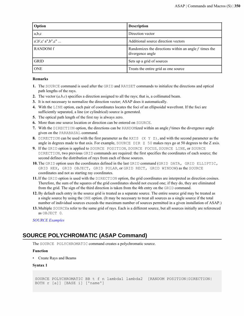
ASAP | Commands and Macros (S) | 350
Option Description
a,b,c Direction vector
a',b',c' a",b",c" ... Additional source direction vectors
RANDOM f Randomizes the directions within an angle f times thedivergence angle
GRID Sets up a grid of sources
ONE Treats the entire grid as one source
Remarks
1. The SOURCE command is used after the GRID and RAYSET commands to initialize the directions and opticalpath lengths of the rays.
2. The vector (a,b,c) specifies a direction assigned to all the rays; that is, a collimated beam.3. It is not necessary to normalize the direction vector; ASAP does it automatically.4. With the LINE option, each pair of coordinates locates the foci of an ellipsoidal wavefront. If the foci are
sufficiently separated, a line (or cylindrical) source is generated.5. The optical path length of the first ray is always zero.6. More than one source location or direction can be entered on SOURCE.7. With the DIRECTION option, the directions can be RANDOMized within an angle f times the divergence angle
given on the PARABASAL command.8. DIRECTION can be used with the first parameter as the AXIS (X Y Z), and with the second parameter as the
angle in degrees made to that axis. For example, SOURCE DIR Z 50 makes rays go at 50 degrees to the Z axis.9. If the GRID option is applied to SOURCE POSITION, SOURCE FOCUS, SOURCE LINE, or SOURCE
DIRECTION, two previous GRID commands are required: the first specifies the coordinates of each source; thesecond defines the distribution of rays from each of those sources.
10. The GRID option uses the coordinates defined in the last GRID command (GRID DATA, GRID ELLIPTIC,GRID HEX, GRID OBJECT, GRID POLAR, or GRID RECT, GRID WINDOW) as the SOURCEcoordinates and not as starting ray coordinates.
11. If the GRID option is used with the DIRECTION option, the grid coordinates are interpreted as direction cosines.Therefore, the sum of the squares of the grid coordinates should not exceed one; if they do, they are eliminatedfrom the grid. The sign of the third direction is taken from the 4th entry on the GRID command.
12. By default each entry in the source grid is treated as a separate source. The entire source grid may be treated asa single source by using the ONE option. (It may be necessary to treat all sources as a single source if the totalnumber of individual sources exceeds the maximum number of sources permitted in a given installation of ASAP.)
13. Multiple SOURCEs refer to the same grid of rays. Each is a different source, but all sources initially are referencedas OBJECT 0.
SOURCE Examples
SOURCE POLYCHROMATIC (ASAP Command)The SOURCE POLYCHROMATIC command creates a polychromatic source.
Function
• Create Rays and Beams
Syntax 1
SOURCE POLYCHROMATIC BB t f n lambda1 lambda2 [RANDOM POSITION|DIRECTION|BOTH r [a]] [BASE i] ['name']
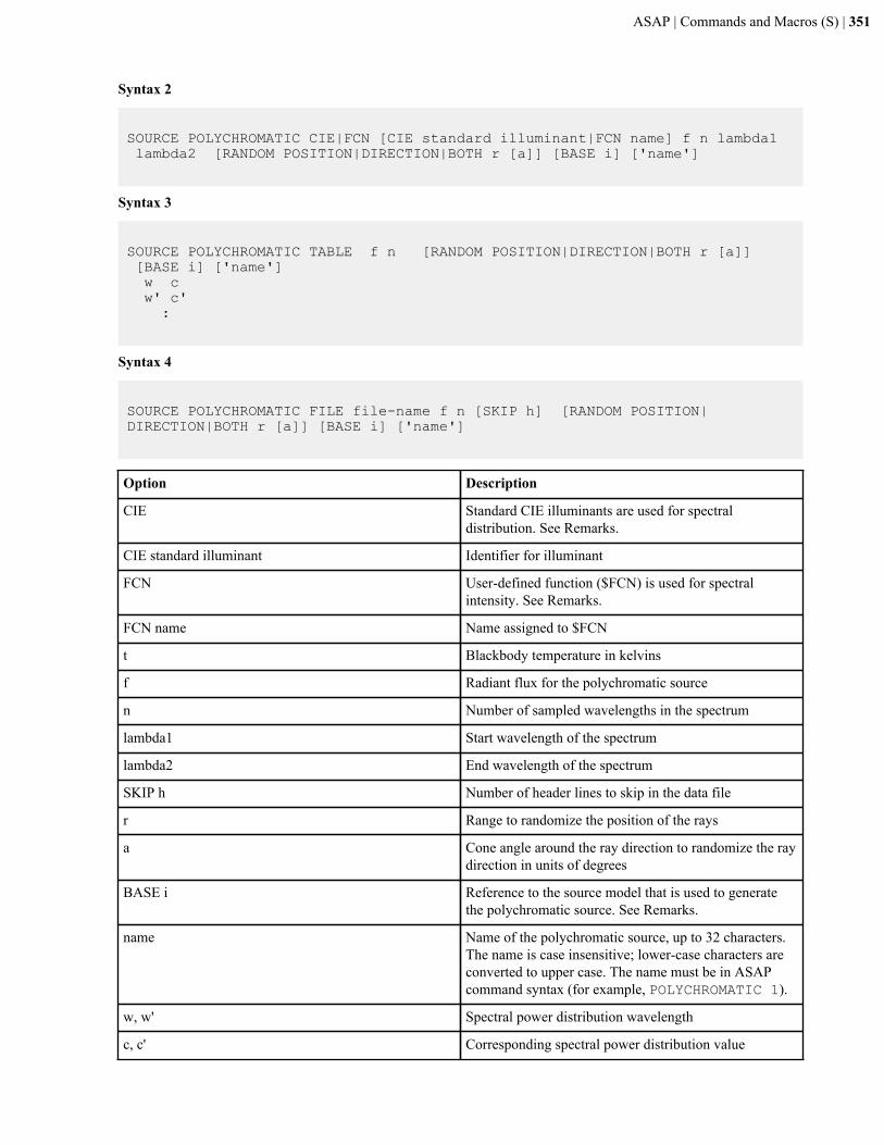
ASAP | Commands and Macros (S) | 351
Syntax 2
SOURCE POLYCHROMATIC CIE|FCN [CIE standard illuminant|FCN name] f n lambda1 lambda2 [RANDOM POSITION|DIRECTION|BOTH r [a]] [BASE i] ['name']
Syntax 3
SOURCE POLYCHROMATIC TABLE f n [RANDOM POSITION|DIRECTION|BOTH r [a]] [BASE i] ['name'] w c w' c' :
Syntax 4
SOURCE POLYCHROMATIC FILE file-name f n [SKIP h] [RANDOM POSITION|DIRECTION|BOTH r [a]] [BASE i] ['name']
Option Description
CIE Standard CIE illuminants are used for spectraldistribution. See Remarks.
CIE standard illuminant Identifier for illuminant
FCN User-defined function ($FCN) is used for spectralintensity. See Remarks.
FCN name Name assigned to $FCN
t Blackbody temperature in kelvins
f Radiant flux for the polychromatic source
n Number of sampled wavelengths in the spectrum
lambda1 Start wavelength of the spectrum
lambda2 End wavelength of the spectrum
SKIP h Number of header lines to skip in the data file
r Range to randomize the position of the rays
a Cone angle around the ray direction to randomize the raydirection in units of degrees
BASE i Reference to the source model that is used to generatethe polychromatic source. See Remarks.
name Name of the polychromatic source, up to 32 characters.The name is case insensitive; lower-case characters areconverted to upper case. The name must be in ASAPcommand syntax (for example, POLYCHROMATIC 1).
w, w' Spectral power distribution wavelength
c, c' Corresponding spectral power distribution value
ASAP | Commands and Macros (S) | 352
Option Description
RANDOM See Remarks.
Remarks
1. The SOURCE POLYCHROMATIC command creates a polychromatic source by duplicating the single-wavelengthsource specified by BASE i (using absolute or relative referencing), or the latest defined single-wavelengthsource at specified sample wavelengths with a proper relative spectral power distribution. A polychromatic sourceconsists of many single-wavelength sources. The single-wavelength source is defined by using commands such as:GRID, SOURCE, or EMITTING. These single wavelength sources may also be modified with ROTATE, SHIFT,or MOVE.
2. Each SOURCE POLYCHROMATIC requires its own baseline source definition. By using the BASE option, a givensource definition can be applied to multiple polychromatic sources. For example:
!!This is the first defined source GRID ELLIPTIC Z 0 -4@1 11 11 SOURCE POSITION 0 0 -5 SOURCE POLYCHROMATIC CIE D50 100.0 97 380 680 'CIE_D50_BUILT_IN' ... SOURCE POLYCHROMATIC CIE D50 100.0 97 380 680 BASE 1 'CIE_D50_BUILT_IN' SOURCE POLYCHROMATIC CIE DTC6500 100.0 107 300 830 BASE 1 'CIE_DTC_6500K_BUILT_IN'
3. By default, the maximum number of allowed polychromatic sources is 50, which can be reset to any number withSET MNPS n. This command must be used before a polychromatic source is defined.
4. The SOURCE POLYCHROMATIC command adds the specified number (n) of single-wavelength sources tothe source list. Be aware that the total number of independent monochromatic sources that are allowed is easilyreached if you are defining a large number of polychromatic sources. The total number (currently 4096) is printedin the command output window by running the DIMENSIONS command.
5. Wavelength must be specified in units of nm for blackbody polychromatic sources and CIE standard illuminants.ASAP automatically converts the nm wavelength to the unit that was set by the last WAVELENGTH command.For other types of polychromatic sources, no wavelength unit is assumed and no automatic wavelength unitconversion takes place.
6. CIE standard illuminants C, D50, D55, D75, and F1 to F12 are supported with tabulated data in 5nm resolution.Linear interpolation is used for higher resolutions.
7. CIE standard illuminants A and D65 are supported with tabulated data in 1nm resolution. Linear interpolation isused for higher resolutions.
8. For an arbitrary CIE D-series illuminant with correlated color temperature of Tc in kelvins, the CIE standardilluminant must be specified as DTCxxxx, where xxxx is the correlated color temperature Tc. The temperaturerange is 5000K to 20,000K.
9. The CIE standard E source is supported and is a uniform source in which the spectral power distribution (SPD) isconstant in the visible spectrum. Any resolution is supported since it is just a constant for the SPD.
10. The wavelength spectrum must be uniformly sampled for a blackbody radiator, all CIE standard illuminants, and$FCN-driven polychromatic sources.
11. The wavelength spectrum that is specified in a table or file for TABLE- and FILE-driven polychromatic sourcescan be sampled at arbitrary intervals. BRO recommends as a best practice to use equal increment wavelengthspacings in your definitions for the SPD.
12. For FILE-driven polychromatic sources, the relative spectral power distribution must be specified in the format ofwavelength and SPD value on each line. The file extension must also be specified (there is no default extension).
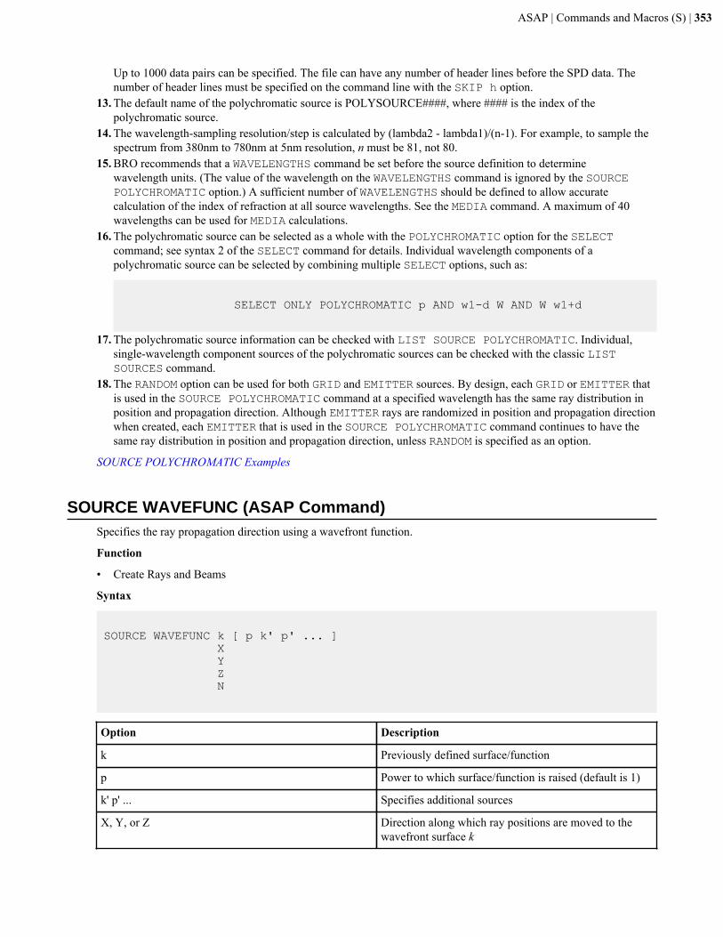
ASAP | Commands and Macros (S) | 353
Up to 1000 data pairs can be specified. The file can have any number of header lines before the SPD data. Thenumber of header lines must be specified on the command line with the SKIP h option.
13. The default name of the polychromatic source is POLYSOURCE####, where #### is the index of thepolychromatic source.
14. The wavelength-sampling resolution/step is calculated by (lambda2 - lambda1)/(n-1). For example, to sample thespectrum from 380nm to 780nm at 5nm resolution, n must be 81, not 80.
15. BRO recommends that a WAVELENGTHS command be set before the source definition to determinewavelength units. (The value of the wavelength on the WAVELENGTHS command is ignored by the SOURCEPOLYCHROMATIC option.) A sufficient number of WAVELENGTHS should be defined to allow accuratecalculation of the index of refraction at all source wavelengths. See the MEDIA command. A maximum of 40wavelengths can be used for MEDIA calculations.
16. The polychromatic source can be selected as a whole with the POLYCHROMATIC option for the SELECTcommand; see syntax 2 of the SELECT command for details. Individual wavelength components of apolychromatic source can be selected by combining multiple SELECT options, such as:
SELECT ONLY POLYCHROMATIC p AND w1-d W AND W w1+d
17. The polychromatic source information can be checked with LIST SOURCE POLYCHROMATIC. Individual,single-wavelength component sources of the polychromatic sources can be checked with the classic LISTSOURCES command.
18. The RANDOM option can be used for both GRID and EMITTER sources. By design, each GRID or EMITTER thatis used in the SOURCE POLYCHROMATIC command at a specified wavelength has the same ray distribution inposition and propagation direction. Although EMITTER rays are randomized in position and propagation directionwhen created, each EMITTER that is used in the SOURCE POLYCHROMATIC command continues to have thesame ray distribution in position and propagation direction, unless RANDOM is specified as an option.
SOURCE POLYCHROMATIC Examples
SOURCE WAVEFUNC (ASAP Command)Specifies the ray propagation direction using a wavefront function.
Function
• Create Rays and Beams
Syntax
SOURCE WAVEFUNC k [ p k' p' ... ] X Y Z N
Option Description
k Previously defined surface/function
p Power to which surface/function is raised (default is 1)
k' p' ... Specifies additional sources
X, Y, or Z Direction along which ray positions are moved to thewavefront surface k
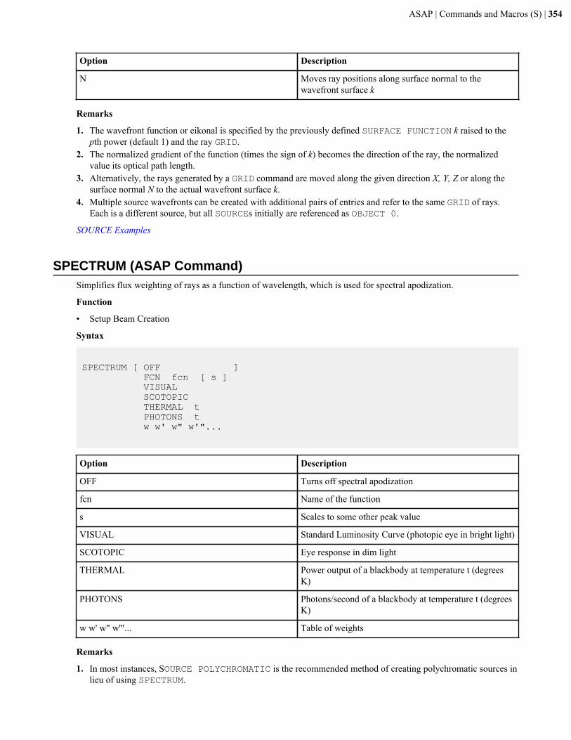
ASAP | Commands and Macros (S) | 354
Option Description
N Moves ray positions along surface normal to thewavefront surface k
Remarks
1. The wavefront function or eikonal is specified by the previously defined SURFACE FUNCTION k raised to thepth power (default 1) and the ray GRID.
2. The normalized gradient of the function (times the sign of k) becomes the direction of the ray, the normalizedvalue its optical path length.
3. Alternatively, the rays generated by a GRID command are moved along the given direction X, Y, Z or along thesurface normal N to the actual wavefront surface k.
4. Multiple source wavefronts can be created with additional pairs of entries and refer to the same GRID of rays.Each is a different source, but all SOURCEs initially are referenced as OBJECT 0.
SOURCE Examples
SPECTRUM (ASAP Command)Simplifies flux weighting of rays as a function of wavelength, which is used for spectral apodization.
Function
• Setup Beam Creation
Syntax
SPECTRUM [ OFF ] FCN fcn [ s ] VISUAL SCOTOPIC THERMAL t PHOTONS t w w' w" w'"...
Option Description
OFF Turns off spectral apodization
fcn Name of the function
s Scales to some other peak value
VISUAL Standard Luminosity Curve (photopic eye in bright light)
SCOTOPIC Eye response in dim light
THERMAL Power output of a blackbody at temperature t (degreesK)
PHOTONS Photons/second of a blackbody at temperature t (degreesK)
w w' w" w'"... Table of weights
Remarks
1. In most instances, SOURCE POLYCHROMATIC is the recommended method of creating polychromatic sources inlieu of using SPECTRUM.
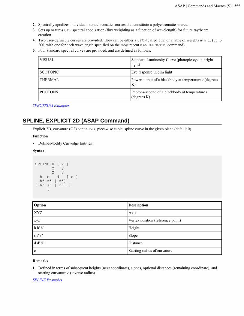
ASAP | Commands and Macros (S) | 355
2. Spectrally apodizes individual monochromatic sources that constitute a polychromatic source.3. Sets up or turns OFF spectral apodization (flux weighting as a function of wavelength) for future ray/beam
creation.4. Two user-definable curves are provided. They can be either a $FCN called fcn or a table of weights w w' ... (up to
200, with one for each wavelength specified on the most recent WAVELENGTHS command).5. Four standard spectral curves are provided, and are defined as follows:
VISUAL Standard Luminosity Curve (photopic eye in brightlight)
SCOTOPIC Eye response in dim light
THERMAL Power output of a blackbody at temperature t (degreesK)
PHOTONS Photons/second of a blackbody at temperature t(degrees K)
SPECTRUM Examples
SPLINE, EXPLICIT 2D (ASAP Command)Explicit 2D, curvature (G2) continuous, piecewise cubic, spline curve in the given plane (default 0).
Function
• Define/Modify Curvedge Entities
Syntax
SPLINE X [ x ] Y y Z z h s d [ c ] h' s' [ d'][ h" s" [ d"] ] :
Option Description
XYZ Axis
xyz Vertex position (reference point)
h h' h" Height
s s' s" Slope
d d' d" Distance
c Starting radius of curvature
Remarks
1. Defined in terms of subsequent heights (next coordinate), slopes, optional distances (remaining coordinate), andstarting curvature c (inverse radius).
SPLINE Examples

ASAP | Commands and Macros (S) | 356
SPLINE, GENERAL 3D (ASAP Command)General 3D piecewise, cubic, spline curve with given reference point (default origin), and defined in terms ofsubsequent relative points and tangent directions (and optional inverse radii of curvatures).
Function
• Define/Modify Curvedge Entities
Syntax
SPLINE [ x y z ] [ CURV ] x y z a, b, c [ k ] x' y' z' a',b',c' [ k' ] [ x" y" z" a",b" c" ] [ k" ] ] :
Option Description
x y z Vertex position (reference point)
CURV Initial radius of curvature at reference point
k k' k" Curvatures at points along the curve
x' y' z' Subsequent point on the curve
a b c, a' b' c' Direction vectors
Remarks
1. If a tangent direction is not provided for any point, one is calculated by finite differences using the adjacent points.Therefore, this command can also be used as an (often better) alternative to POINTS followed by SMOOTH 3(although it does create a curve with three times as many Bezier points).
SPLINE Examples
SPLIT (ASAP Command)Controls the number of times a ray may be split into specular components.
Function
• Create/Modify Objects• Setup Trace
Syntax
SPLIT [ n ] [ MONTECARLO ] [ 'c' ] TRAN REFL NORM OFF ALL
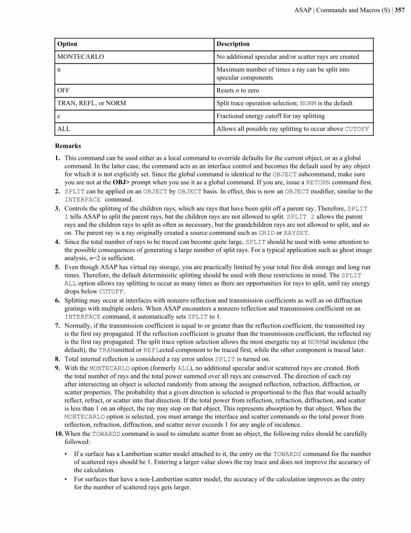
ASAP | Commands and Macros (S) | 357
Option Description
MONTECARLO No additional specular and/or scatter rays are created
n Maximum number of times a ray can be split intospecular components
OFF Resets n to zero
TRAN, REFL, or NORM Split trace operation selection; NORM is the default
c Fractional energy cutoff for ray splitting
ALL Allows all possible ray splitting to occur above CUTOFF
Remarks
1. This command can be used either as a local command to override defaults for the current object, or as a globalcommand. In the latter case, the command acts as an interface control and becomes the default used by any objectfor which it is not explicitly set. Since the global command is identical to the OBJECT subcommand, make sureyou are not at the OBJ> prompt when you use it as a global command. If you are, issue a RETURN command first.
2. SPLIT can be applied on an OBJECT by OBJECT basis. In effect, this is now an OBJECT modifier, similar to theINTERFACE command.
3. Controls the splitting of the children rays, which are rays that have been split off a parent ray. Therefore, SPLIT1 tells ASAP to split the parent rays, but the children rays are not allowed to split. SPLIT 2 allows the parentrays and the children rays to split as often as necessary, but the grandchildren rays are not allowed to split, and soon. The parent ray is a ray originally created a source command such as GRID or RAYSET.
4. Since the total number of rays to be traced can become quite large, SPLIT should be used with some attention tothe possible consequences of generating a large number of split rays. For a typical application such as ghost imageanalysis, n=2 is sufficient.
5. Even though ASAP has virtual ray storage, you are practically limited by your total free disk storage and long runtimes. Therefore, the default deterministic splitting should be used with these restrictions in mind. The SPLITALL option allows ray splitting to occur as many times as there are opportunities for rays to split, until ray energydrops below CUTOFF.
6. Splitting may occur at interfaces with nonzero reflection and transmission coefficients as well as on diffractiongratings with multiple orders. When ASAP encounters a nonzero reflection and transmission coefficient on anINTERFACE command, it automatically sets SPLIT to 1.
7. Normally, if the transmission coefficient is equal to or greater than the reflection coefficient, the transmitted rayis the first ray propagated. If the reflection coefficient is greater than the transmission coefficient, the reflected rayis the first ray propagated. The split trace option selection allows the most energetic ray at NORMal incidence (thedefault), the TRANsmitted or REFLected component to be traced first, while the other component is traced later.
8. Total internal reflection is considered a ray error unless SPLIT is turned on.9. With the MONTECARLO option (formerly ALL), no additional specular and/or scattered rays are created. Both
the total number of rays and the total power summed over all rays are conserved. The direction of each rayafter intersecting an object is selected randomly from among the assigned reflection, refraction, diffraction, orscatter properties. The probability that a given direction is selected is proportional to the flux that would actuallyreflect, refract, or scatter into that direction. If the total power from reflection, refraction, diffraction, and scatteris less than 1 on an object, the ray may stop on that object. This represents absorption by that object. When theMONTECARLO option is selected, you must arrange the interface and scatter commands so the total power fromreflection, refraction, diffraction, and scatter never exceeds 1 for any angle of incidence.
10. When the TOWARDS command is used to simulate scatter from an object, the following rules should be carefullyfollowed:
• If a surface has a Lambertian scatter model attached to it, the entry on the TOWARDS command for the numberof scattered rays should be 1. Entering a larger value slows the ray trace and does not improve the accuracy ofthe calculation.
• For surfaces that have a non-Lambertian scatter model, the accuracy of the calculation improves as the entryfor the number of scattered rays gets larger.
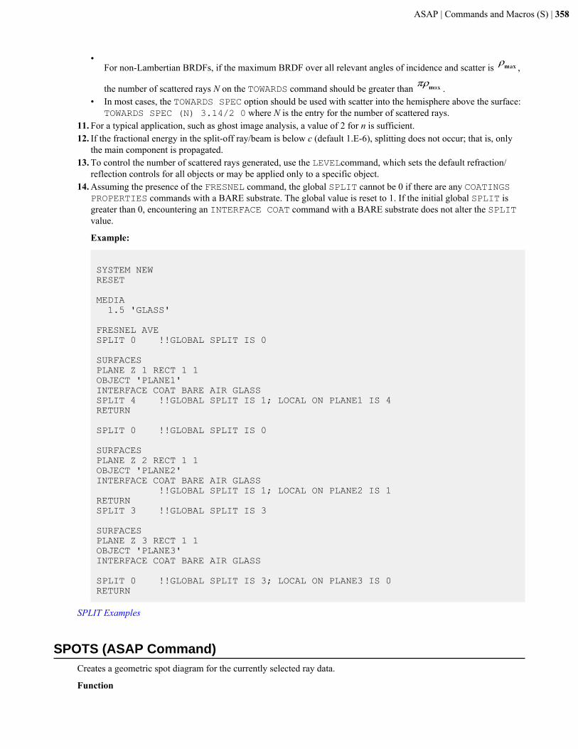
ASAP | Commands and Macros (S) | 358
•For non-Lambertian BRDFs, if the maximum BRDF over all relevant angles of incidence and scatter is ,
the number of scattered rays N on the TOWARDS command should be greater than .• In most cases, the TOWARDS SPEC option should be used with scatter into the hemisphere above the surface:
TOWARDS SPEC (N) 3.14/2 0 where N is the entry for the number of scattered rays.11. For a typical application, such as ghost image analysis, a value of 2 for n is sufficient.12. If the fractional energy in the split-off ray/beam is below c (default 1.E-6), splitting does not occur; that is, only
the main component is propagated.13. To control the number of scattered rays generated, use the LEVELcommand, which sets the default refraction/
reflection controls for all objects or may be applied only to a specific object.14. Assuming the presence of the FRESNEL command, the global SPLIT cannot be 0 if there are any COATINGS
PROPERTIES commands with a BARE substrate. The global value is reset to 1. If the initial global SPLIT isgreater than 0, encountering an INTERFACE COAT command with a BARE substrate does not alter the SPLITvalue.
Example:
SYSTEM NEWRESET
MEDIA 1.5 'GLASS'
FRESNEL AVESPLIT 0 !!GLOBAL SPLIT IS 0
SURFACES PLANE Z 1 RECT 1 1OBJECT 'PLANE1'INTERFACE COAT BARE AIR GLASSSPLIT 4 !!GLOBAL SPLIT IS 1; LOCAL ON PLANE1 IS 4RETURN
SPLIT 0 !!GLOBAL SPLIT IS 0
SURFACES PLANE Z 2 RECT 1 1OBJECT 'PLANE2'INTERFACE COAT BARE AIR GLASS !!GLOBAL SPLIT IS 1; LOCAL ON PLANE2 IS 1RETURNSPLIT 3 !!GLOBAL SPLIT IS 3
SURFACES PLANE Z 3 RECT 1 1OBJECT 'PLANE3'INTERFACE COAT BARE AIR GLASS SPLIT 0 !!GLOBAL SPLIT IS 3; LOCAL ON PLANE3 IS 0RETURN
SPLIT Examples
SPOTS (ASAP Command)Creates a geometric spot diagram for the currently selected ray data.
Function
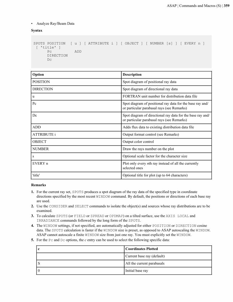
ASAP | Commands and Macros (S) | 359
• Analyze Ray/Beam Data
Syntax
SPOTS POSITION [ u ] [ ATTRIBUTE i ] [ OBJECT ] [ NUMBER [s] ] [ EVERY n ] [ 'title' ] Pc ADD DIRECTION Dc
Option Description
POSITION Spot diagram of positional ray data
DIRECTION Spot diagram of directional ray data
u FORTRAN unit number for distribution data file
Pc Spot diagram of positional ray data for the base ray and/or particular parabasal rays (see Remarks)
Dc Spot diagram of directional ray data for the base ray and/or particular parabasal rays (see Remarks)
ADD Adds flux data to existing distribution data file
ATTRIBUTE i Output format control (see Remarks)
OBJECT Output color control
NUMBER Draw the rays number on the plot
s Optional scale factor for the character size
EVERY n Plot only every nth ray instead of all the currentlyselected ones
'title' Optional title for plot (up to 64 characters)
Remarks
1. For the current ray set, SPOTS produces a spot diagram of the ray data of the specified type in coordinatedirections specified by the most recent WINDOW command. By default, the positions or directions of each base rayare used.
2. Use the CONSIDER and SELECT commands to isolate the object(s) and sources whose ray distributions are to beexamined.
3. To calculate SPOTS (or FIELD or SPREAD or OPDMAP) on a tilted surface, use the AXIS LOCAL andIRRADIANCE commands followed by the long form of the SPOTS.
4. The WINDOW settings, if not specified, are automatically adjusted for either POSITION or DIRECTION cosinedata. The SPOTS calculation is faster if the WINDOW size is preset, as opposed to ASAP autoscaling the WINDOW.ASAP cannot autoscale a finite WINDOW size from just one ray. You must explicitly set the WINDOW.
5. For the Pc and Dc options, the c entry can be used to select the following specific data:
c Coordinates Plotted
Current base ray (default)
S All the current parabasals
0 Initial base ray
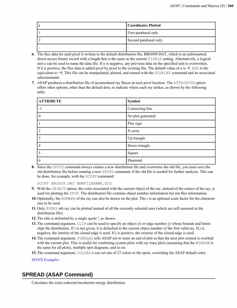
ASAP | Commands and Macros (S) | 360
c Coordinates Plotted
1 First parabasal only
2 Second parabasal only
: :
6. The flux data for each pixel is written to the default distribution file, BRO009.DAT, which is an unformatted,direct-access binary record with a length that is the same as the current PIXELS setting. Alternatively, a logicalunit u can be used to name the data file. If u is negative, any previous data on the specified unit is overwritten.If it is positive, the flux data is added pixel by pixel to the existing file. The default value of u is -9. ADD is theequivalent to +9. This file can be manipulated, plotted, and named with the DISPLAY command and its associatedsubcommands.
7. ASAP produces a distribution file of accumulated ray fluxes at each pixel location. The ATTRIBUTE optionoffers other options, other than the default dots, to indicate where each ray strikes, as shown by the followingtable.
ATTRIBUTE Symbol
-1 Connecting line
0 No plot generated
1 Plus sign
2 X cross
3 Up triangle
4 Down triangle
5 Square
6 Diamond
8. Since the SPOTS command always creates a new distribution file and overwrites the old file, you must save theold distribution file before running a new SPOTS command, if the old file is needed for further analysis. This canbe done, for example, with the $COPY command:
$COPY BRO009.DAT NEWFILENAME.DIS9. With the OBJECT option, the color associated with the current object of the ray, instead of the source of the ray, is
used for plotting the SPOT. The distribution file contains object number information but not flux information.10. Optionally, the NUMBER of the ray can also be drawn on the plot. The s is an optional scale factor for the character
size to be used.11. Only EVERY nth ray can be plotted instead of all the currently selected ones (which are still summed in the
distribution file).12. The title is delimited by a single quote ', as shown.13. The command argument, CLIP can be used to specify an object (i) or edge number (j) whose bounds and limits
clips the distribution. If i is not given, it is defaulted to the current object number of the first valid ray. If j isnegative, the interior of the closed edge is used. If j is positive, the exterior of the closed edge is used.
14. The command argument, OVERLAY tells ASAP not to issue an end of plot so that the next plot created is overlaidwith the current plot. This is useful for combining system plots with ray trace plots (assuming that the WINDOW isthe same for all plots), multiple spot diagrams, and so on.
15. The command argument, COLORS n can set one of 27 colors to the spots, overriding the ASAP default color.
SPOTS Examples
SPREAD (ASAP Command)Calculates the exact coherent/incoherent energy distribution.
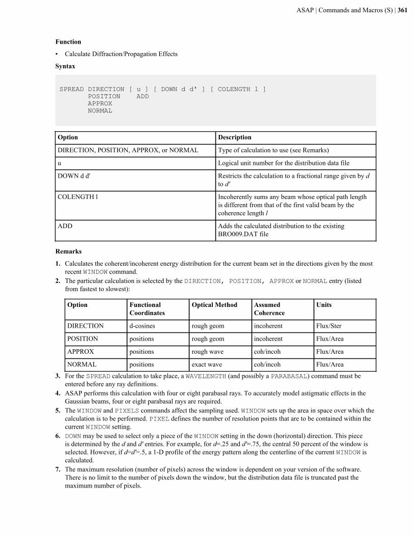
ASAP | Commands and Macros (S) | 361
Function
• Calculate Diffraction/Propagation Effects
Syntax
SPREAD DIRECTION [ u ] [ DOWN d d' ] [ COLENGTH l ] POSITION ADD APPROX NORMAL
Option Description
DIRECTION, POSITION, APPROX, or NORMAL Type of calculation to use (see Remarks)
u Logical unit number for the distribution data file
DOWN d d' Restricts the calculation to a fractional range given by dto d'
COLENGTH l Incoherently sums any beam whose optical path lengthis different from that of the first valid beam by thecoherence length l
ADD Adds the calculated distribution to the existingBRO009.DAT file
Remarks
1. Calculates the coherent/incoherent energy distribution for the current beam set in the directions given by the mostrecent WINDOW command.
2. The particular calculation is selected by the DIRECTION, POSITION, APPROX or NORMAL entry (listedfrom fastest to slowest):
Option FunctionalCoordinates
Optical Method AssumedCoherence
Units
DIRECTION d-cosines rough geom incoherent Flux/Ster
POSITION positions rough geom incoherent Flux/Area
APPROX positions rough wave coh/incoh Flux/Area
NORMAL positions exact wave coh/incoh Flux/Area
3. For the SPREAD calculation to take place, a WAVELENGTH (and possibly a PARABASAL) command must beentered before any ray definitions.
4. ASAP performs this calculation with four or eight parabasal rays. To accurately model astigmatic effects in theGaussian beams, four or eight parabasal rays are required.
5. The WINDOW and PIXELS commands affect the sampling used. WINDOW sets up the area in space over which thecalculation is to be performed. PIXEL defines the number of resolution points that are to be contained within thecurrent WINDOW setting.
6. DOWN may be used to select only a piece of the WINDOW setting in the down (horizontal) direction. This pieceis determined by the d and d' entries. For example, for d=.25 and d'=.75, the central 50 percent of the window isselected. However, if d=d'=.5, a 1-D profile of the energy pattern along the centerline of the current WINDOW iscalculated.
7. The maximum resolution (number of pixels) across the window is dependent on your version of the software.There is no limit to the number of pixels down the window, but the distribution data file is truncated past themaximum number of pixels.
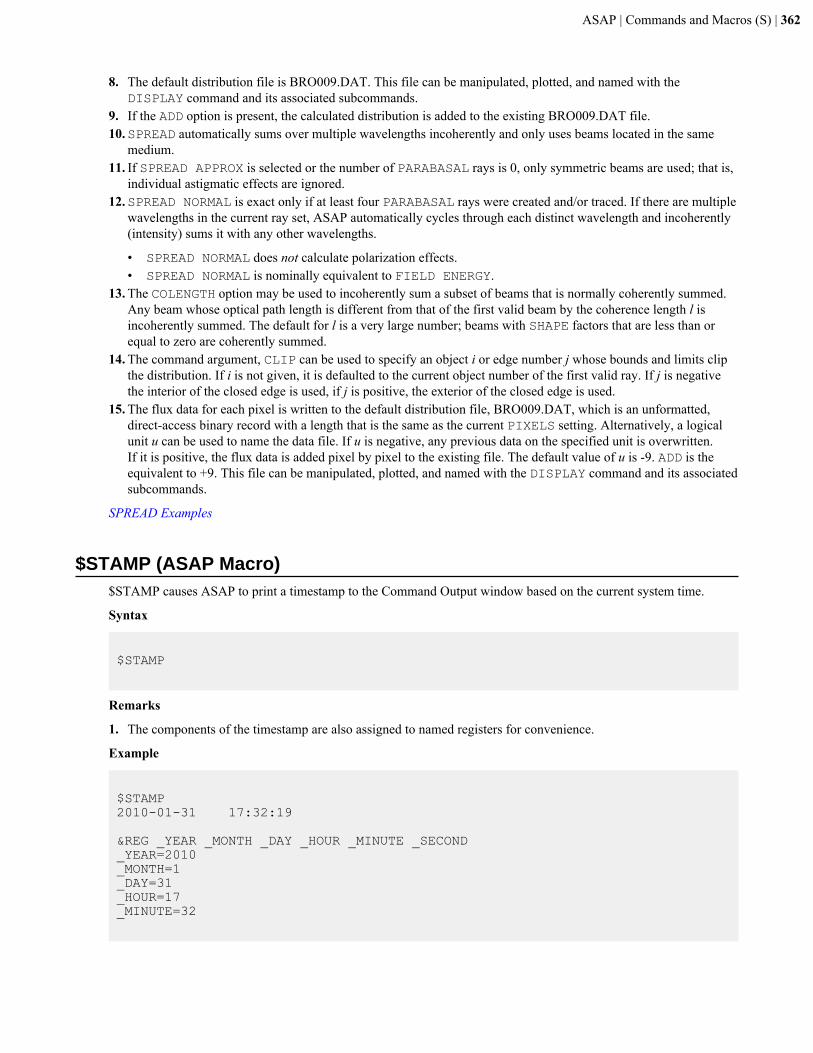
ASAP | Commands and Macros (S) | 362
8. The default distribution file is BRO009.DAT. This file can be manipulated, plotted, and named with theDISPLAY command and its associated subcommands.
9. If the ADD option is present, the calculated distribution is added to the existing BRO009.DAT file.10.SPREAD automatically sums over multiple wavelengths incoherently and only uses beams located in the same
medium.11. If SPREAD APPROX is selected or the number of PARABASAL rays is 0, only symmetric beams are used; that is,
individual astigmatic effects are ignored.12.SPREAD NORMAL is exact only if at least four PARABASAL rays were created and/or traced. If there are multiple
wavelengths in the current ray set, ASAP automatically cycles through each distinct wavelength and incoherently(intensity) sums it with any other wavelengths.
• SPREAD NORMAL does not calculate polarization effects.• SPREAD NORMAL is nominally equivalent to FIELD ENERGY.
13. The COLENGTH option may be used to incoherently sum a subset of beams that is normally coherently summed.Any beam whose optical path length is different from that of the first valid beam by the coherence length l isincoherently summed. The default for l is a very large number; beams with SHAPE factors that are less than orequal to zero are coherently summed.
14. The command argument, CLIP can be used to specify an object i or edge number j whose bounds and limits clipthe distribution. If i is not given, it is defaulted to the current object number of the first valid ray. If j is negativethe interior of the closed edge is used, if j is positive, the exterior of the closed edge is used.
15. The flux data for each pixel is written to the default distribution file, BRO009.DAT, which is an unformatted,direct-access binary record with a length that is the same as the current PIXELS setting. Alternatively, a logicalunit u can be used to name the data file. If u is negative, any previous data on the specified unit is overwritten.If it is positive, the flux data is added pixel by pixel to the existing file. The default value of u is -9. ADD is theequivalent to +9. This file can be manipulated, plotted, and named with the DISPLAY command and its associatedsubcommands.
SPREAD Examples
$STAMP (ASAP Macro)$STAMP causes ASAP to print a timestamp to the Command Output window based on the current system time.
Syntax
$STAMP
Remarks
1. The components of the timestamp are also assigned to named registers for convenience.
Example
$STAMP2010-01-31 17:32:19 ® _YEAR _MONTH _DAY _HOUR _MINUTE _SECOND_YEAR=2010_MONTH=1_DAY=31 _HOUR=17_MINUTE=32
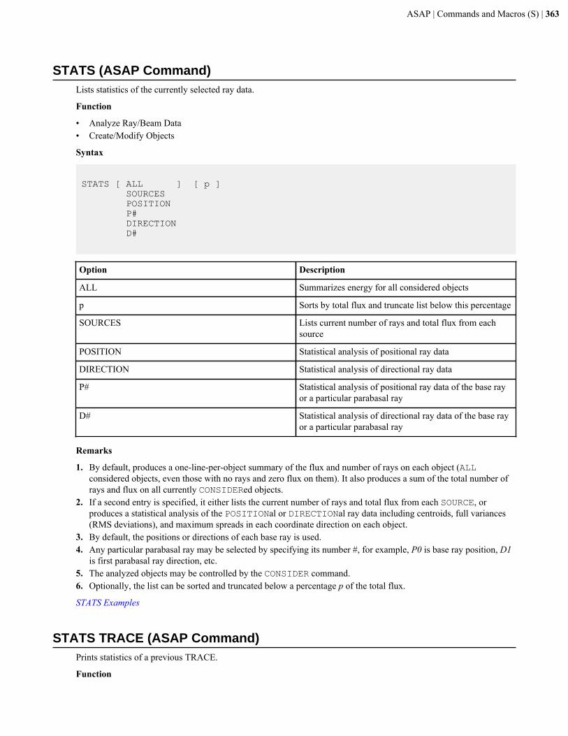
ASAP | Commands and Macros (S) | 363
STATS (ASAP Command)Lists statistics of the currently selected ray data.
Function
• Analyze Ray/Beam Data• Create/Modify Objects
Syntax
STATS [ ALL ] [ p ] SOURCES POSITION P# DIRECTION D#
Option Description
ALL Summarizes energy for all considered objects
p Sorts by total flux and truncate list below this percentage
SOURCES Lists current number of rays and total flux from eachsource
POSITION Statistical analysis of positional ray data
DIRECTION Statistical analysis of directional ray data
P# Statistical analysis of positional ray data of the base rayor a particular parabasal ray
D# Statistical analysis of directional ray data of the base rayor a particular parabasal ray
Remarks
1. By default, produces a one-line-per-object summary of the flux and number of rays on each object (ALLconsidered objects, even those with no rays and zero flux on them). It also produces a sum of the total number ofrays and flux on all currently CONSIDERed objects.
2. If a second entry is specified, it either lists the current number of rays and total flux from each SOURCE, orproduces a statistical analysis of the POSITIONal or DIRECTIONal ray data including centroids, full variances(RMS deviations), and maximum spreads in each coordinate direction on each object.
3. By default, the positions or directions of each base ray is used.4. Any particular parabasal ray may be selected by specifying its number #, for example, P0 is base ray position, D1
is first parabasal ray direction, etc.5. The analyzed objects may be controlled by the CONSIDER command.6. Optionally, the list can be sorted and truncated below a percentage p of the total flux.
STATS Examples
STATS TRACE (ASAP Command)Prints statistics of a previous TRACE.
Function
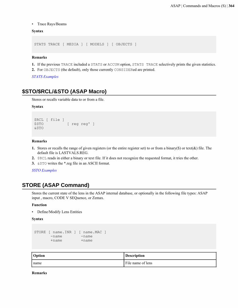
ASAP | Commands and Macros (S) | 364
• Trace Rays/Beams
Syntax
STATS TRACE [ MEDIA ] [ MODELS ] [ OBJECTS ]
Remarks
1. If the previous TRACE included a STATS or ACCUM option, STATS TRACE selectively prints the given statistics.2. For OBJECTS (the default), only those currently CONSIDERed are printed.
STATS Examples
$STO/$RCL/&STO (ASAP Macro)Stores or recalls variable data to or from a file.
Syntax
$RCL [ file ]$STO [ reg reg' ]&STO
Remarks
1. Stores or recalls the range of given registers (or the entire register set) to or from a binary($) or text(&) file. Thedefault file is LASTVALS.REG.
2. $RCL reads in either a binary or text file. If it does not recognize the requested format, it tries the other.3. &STO writes the *.reg file in an ASCII format.
$STO Examples
STORE (ASAP Command)Stores the current state of the lens in the ASAP internal database, or optionally in the following file types: ASAPinput , macro, CODE V SEQuence, or Zemax.
Function
• Define/Modify Lens Entities
Syntax
STORE [ name.INR ] [ name.MAC ] -name -name +name +name
Option Description
name File name of lens
Remarks
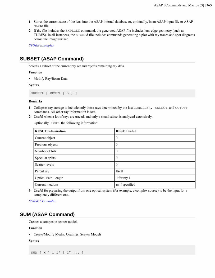
ASAP | Commands and Macros (S) | 365
1. Stores the current state of the lens into the ASAP internal database or, optionally, in an ASAP input file or ASAPMACro file.
2. If the file includes the EXPLODE command, the generated ASAP file includes lens edge geometry (such asTUBES). In all instances, the STOREd file includes commands generating a plot with ray traces and spot diagramsacross the image surface.
STORE Examples
SUBSET (ASAP Command)Selects a subset of the current ray set and rejects remaining ray data.
Function
• Modify Ray/Beam Data
Syntax
SUBSET [ RESET [ m ] ]
Remarks
1. Collapses ray storage to include only those rays determined by the last CONSIDER, SELECT, and CUTOFFcommands. All other ray information is lost.
2. Useful when a lot of rays are traced, and only a small subset is analyzed extensively.
Optionally RESET the following information:
RESET Information RESET value
Current object 0
Previous objects 0
Number of hits 0
Specular splits 0
Scatter levels 0
Parent ray Itself
Optical Path Length 0 for ray 1
Current medium m if specified
3. Useful for preparing the output from one optical system (for example, a complex source) to be the input for acompletely different one.
SUBSET Examples
SUM (ASAP Command)Creates a composite scatter model.
Function
• Create/Modify Media, Coatings, Scatter Models
Syntax
SUM [ X ] i i' [ i" ... ]
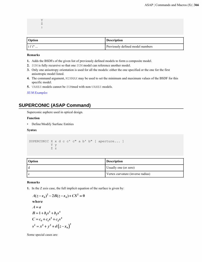
ASAP | Commands and Macros (S) | 366
Y Z :
Option Description
i i' i" ... Previously defined model numbers
Remarks
1. Adds the BSDFs of the given list of previously defined models to form a composite model.2. SUM is fully recursive so that one SUM model can reference another model.3. Only one anisotropy orientation is used for all the models: either the one specified or the one for the first
anisotropic model listed.4. The command argument, MINMAX may be used to set the minimum and maximum values of the BSDF for this
specific model.5. VANES models cannot be SUMmed with non-VANES models.
SUM Examples
SUPERCONIC (ASAP Command)Superconic asphere used in optical design.
Function
• Define/Modify Surfunc Entities
Syntax
SUPERCONIC X x d c c' c" a b' b" [ aperture... ] Y y Z z
Option Description
d Usually one (or zero)
c Vertex curvature (inverse radius)
Remarks
1. In the Z axis case, the full implicit equation of the surface is given by:
Some special cases are:
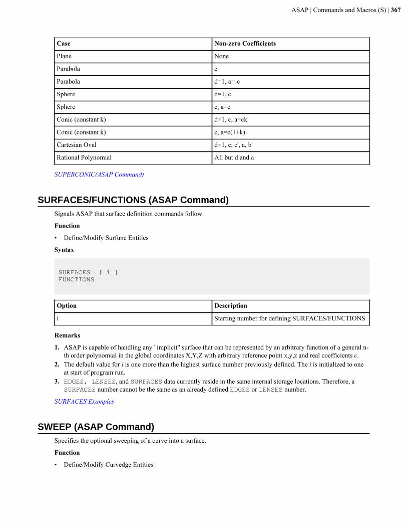
ASAP | Commands and Macros (S) | 367
Case Non-zero Coefficients
Plane None
Parabola c
Parabola d=1, a=-c
Sphere d=1, c
Sphere c, a=c
Conic (constant k) d=1, c, a=ck
Conic (constant k) c, a=c(1+k)
Cartesian Oval d=1, c, c', a, b'
Rational Polynomial All but d and a
SUPERCONIC(ASAP Command)
SURFACES/FUNCTIONS (ASAP Command)Signals ASAP that surface definition commands follow.
Function
• Define/Modify Surfunc Entities
Syntax
SURFACES [ i ]FUNCTIONS
Option Description
i Starting number for defining SURFACES/FUNCTIONS
Remarks
1. ASAP is capable of handling any "implicit" surface that can be represented by an arbitrary function of a general n-th order polynomial in the global coordinates X,Y,Z with arbitrary reference point x,y,z and real coefficients c.
2. The default value for i is one more than the highest surface number previously defined. The i is initialized to oneat start of program run.
3. EDGES, LENSES, and SURFACES data currently reside in the same internal storage locations. Therefore, aSURFACES number cannot be the same as an already defined EDGES or LENSES number.
SURFACES Examples
SWEEP (ASAP Command)Specifies the optional sweeping of a curve into a surface.
Function
• Define/Modify Curvedge Entities
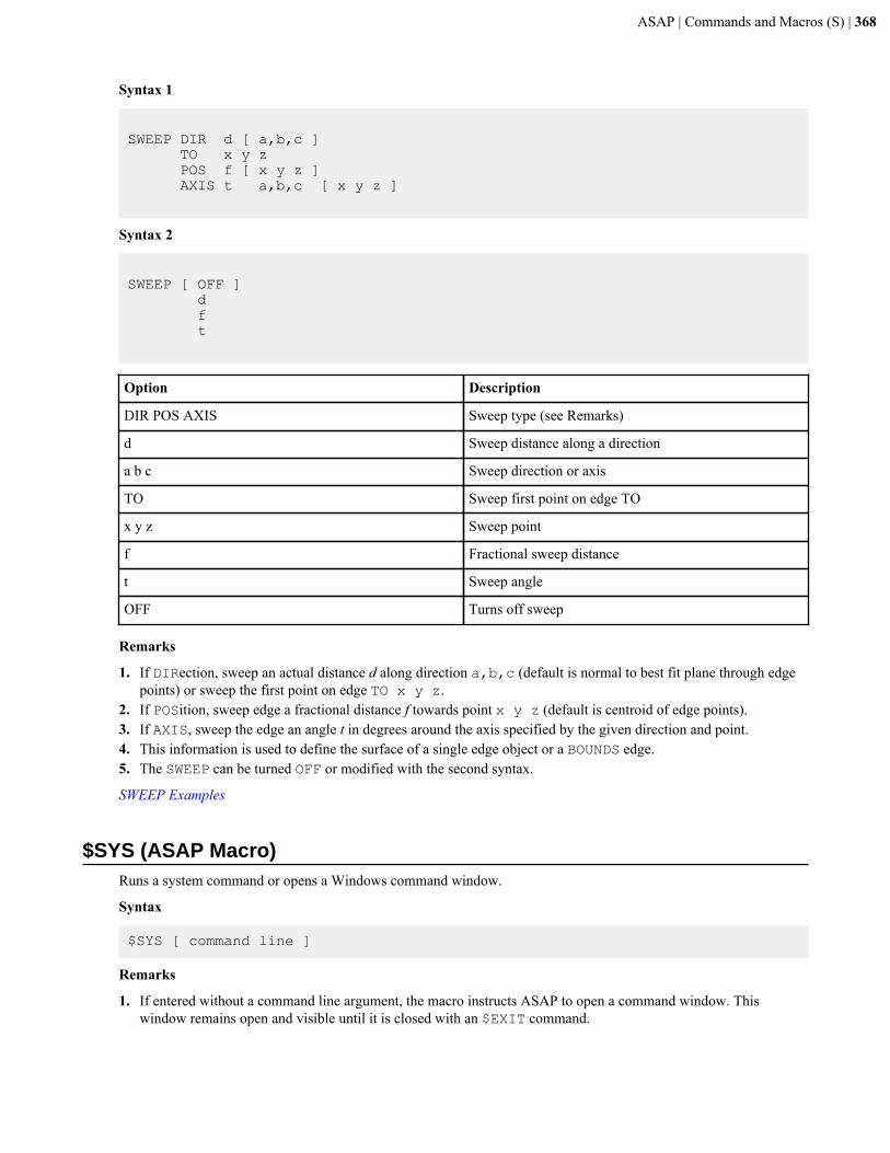
ASAP | Commands and Macros (S) | 368
Syntax 1
SWEEP DIR d [ a,b,c ] TO x y z POS f [ x y z ] AXIS t a,b,c [ x y z ]
Syntax 2
SWEEP [ OFF ] d f t
Option Description
DIR POS AXIS Sweep type (see Remarks)
d Sweep distance along a direction
a b c Sweep direction or axis
TO Sweep first point on edge TO
x y z Sweep point
f Fractional sweep distance
t Sweep angle
OFF Turns off sweep
Remarks
1. If DIRection, sweep an actual distance d along direction a,b,c (default is normal to best fit plane through edgepoints) or sweep the first point on edge TO x y z.
2. If POSition, sweep edge a fractional distance f towards point x y z (default is centroid of edge points).3. If AXIS, sweep the edge an angle t in degrees around the axis specified by the given direction and point.4. This information is used to define the surface of a single edge object or a BOUNDS edge.5. The SWEEP can be turned OFF or modified with the second syntax.
SWEEP Examples
$SYS (ASAP Macro)Runs a system command or opens a Windows command window.
Syntax
$SYS [ command line ]
Remarks
1. If entered without a command line argument, the macro instructs ASAP to open a command window. Thiswindow remains open and visible until it is closed with an $EXIT command.
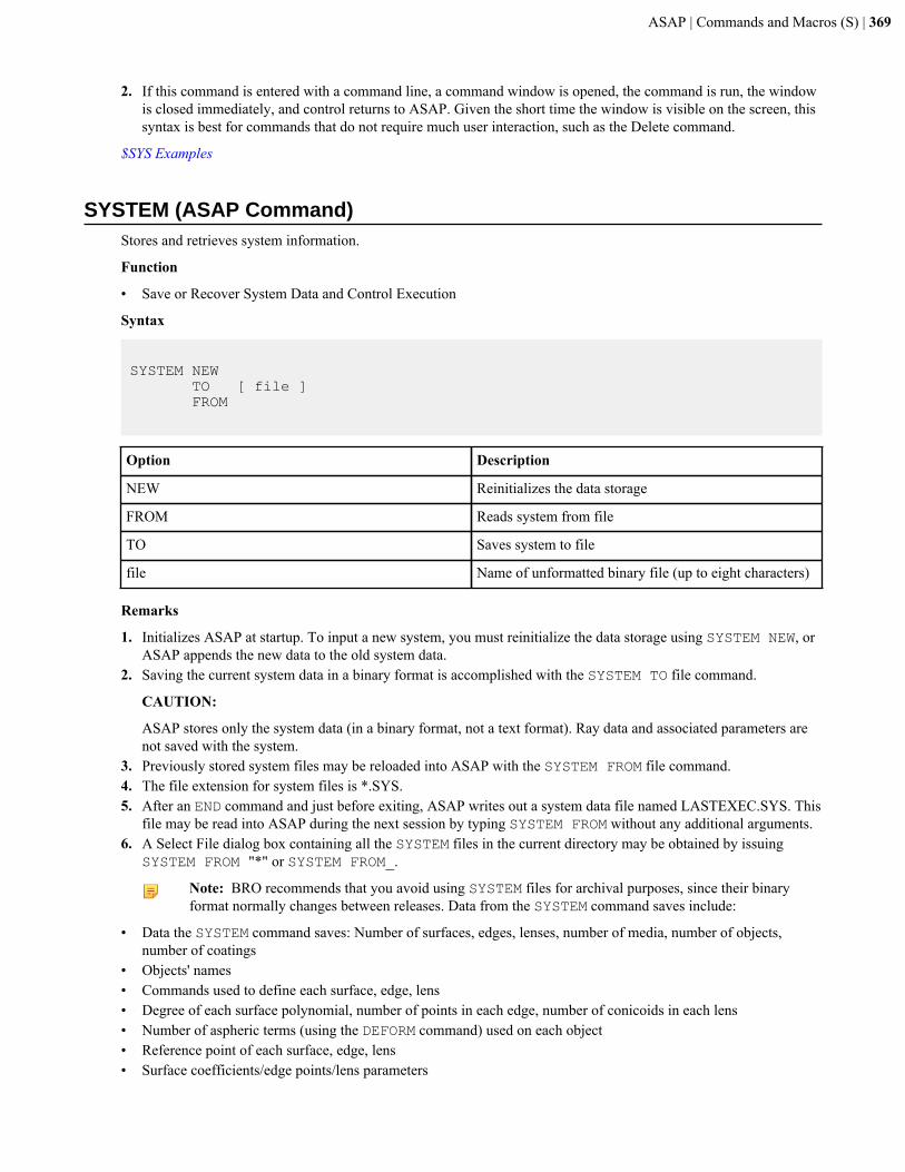
ASAP | Commands and Macros (S) | 369
2. If this command is entered with a command line, a command window is opened, the command is run, the windowis closed immediately, and control returns to ASAP. Given the short time the window is visible on the screen, thissyntax is best for commands that do not require much user interaction, such as the Delete command.
$SYS Examples
SYSTEM (ASAP Command)Stores and retrieves system information.
Function
• Save or Recover System Data and Control Execution
Syntax
SYSTEM NEW TO [ file ] FROM
Option Description
NEW Reinitializes the data storage
FROM Reads system from file
TO Saves system to file
file Name of unformatted binary file (up to eight characters)
Remarks
1. Initializes ASAP at startup. To input a new system, you must reinitialize the data storage using SYSTEM NEW, orASAP appends the new data to the old system data.
2. Saving the current system data in a binary format is accomplished with the SYSTEM TO file command.
CAUTION:
ASAP stores only the system data (in a binary format, not a text format). Ray data and associated parameters arenot saved with the system.
3. Previously stored system files may be reloaded into ASAP with the SYSTEM FROM file command.4. The file extension for system files is *.SYS.5. After an END command and just before exiting, ASAP writes out a system data file named LASTEXEC.SYS. This
file may be read into ASAP during the next session by typing SYSTEM FROM without any additional arguments.6. A Select File dialog box containing all the SYSTEM files in the current directory may be obtained by issuing
SYSTEM FROM "*" or SYSTEM FROM_.
Note: BRO recommends that you avoid using SYSTEM files for archival purposes, since their binaryformat normally changes between releases. Data from the SYSTEM command saves include:
• Data the SYSTEM command saves: Number of surfaces, edges, lenses, number of media, number of objects,number of coatings
• Objects' names• Commands used to define each surface, edge, lens• Degree of each surface polynomial, number of points in each edge, number of conicoids in each lens• Number of aspheric terms (using the DEFORM command) used on each object• Reference point of each surface, edge, lens• Surface coefficients/edge points/lens parameters

ASAP | Commands and Macros (S) | 370
• Multiple and array surface data• Test points• LOCAL data (including transformation matrices and others)• Refractive index and absorption data• GRIN data• Names of MEDIA• COATING prescription data• OBJECT status (from CONSIDER command)• LIMITS Main data• BOUNDed surface data• Real/complex reflection/transmission coefficients• INTERFACE media numbers• Diffractive/holographic optic INTERFACE data• Object SEARCH strategy data• INTERFACE scatter data (RMS heights, slopes, BSDFs, RMS roughnesses, important areas, backscatter data and
others)• Current WAVELENGTHS, UNITs, and wavelengths used to define dispersive MEDIA• $FCNs needed to create geometry
SYSTEM Examples
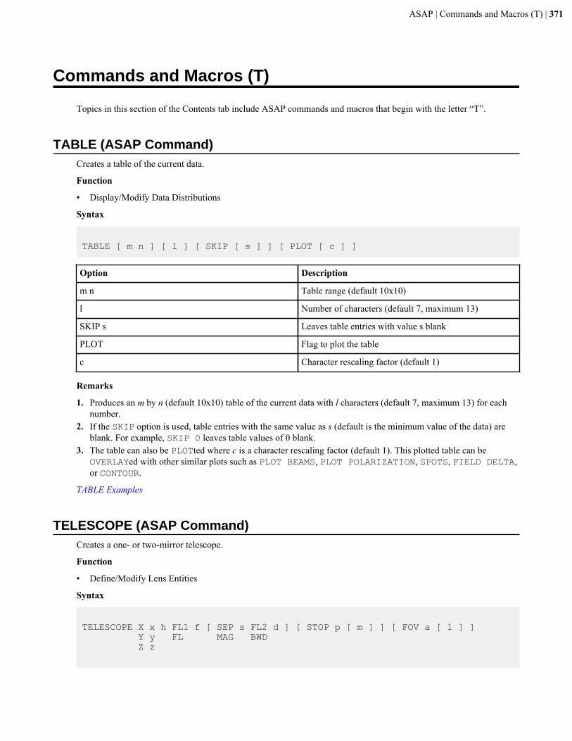
ASAP | Commands and Macros (T) | 371
Commands and Macros (T)
Topics in this section of the Contents tab include ASAP commands and macros that begin with the letter “T”.
TABLE (ASAP Command)Creates a table of the current data.
Function
• Display/Modify Data Distributions
Syntax
TABLE [ m n ] [ l ] [ SKIP [ s ] ] [ PLOT [ c ] ]
Option Description
m n Table range (default 10x10)
l Number of characters (default 7, maximum 13)
SKIP s Leaves table entries with value s blank
PLOT Flag to plot the table
c Character rescaling factor (default 1)
Remarks
1. Produces an m by n (default 10x10) table of the current data with l characters (default 7, maximum 13) for eachnumber.
2. If the SKIP option is used, table entries with the same value as s (default is the minimum value of the data) areblank. For example, SKIP 0 leaves table values of 0 blank.
3. The table can also be PLOTted where c is a character rescaling factor (default 1). This plotted table can beOVERLAYed with other similar plots such as PLOT BEAMS, PLOT POLARIZATION, SPOTS, FIELD DELTA,or CONTOUR.
TABLE Examples
TELESCOPE (ASAP Command)Creates a one- or two-mirror telescope.
Function
• Define/Modify Lens Entities
Syntax
TELESCOPE X x h FL1 f [ SEP s FL2 d ] [ STOP p [ m ] ] [ FOV a [ l ] ] Y y FL MAG BWD Z z
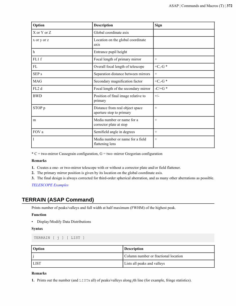
ASAP | Commands and Macros (T) | 372
Option Description Sign
X or Y or Z Global coordinate axis
x or y or z Location on the global coordinateaxis
h Entrance pupil height
FL1 f Focal length of primary mirror +
FL Overall focal length of telescope +C,-G *
SEP s Separation distance between mirrors +
MAG Secondary magnification factor +C,-G *
FL2 d Focal length of the secondary mirror -C/+G *
BWD Position of final image relative toprimary
+/-
STOP p Distance from real object spaceaperture stop to primary
+
m Media number or name for acorrector plate at stop
+
FOV a Semifield angle in degrees +
l Media number or name for a fieldflattening lens
+
* C = two-mirror Cassegrain configuration, G = two–mirror Gregorian configuration
Remarks
1. Creates a one- or two-mirror telescope with or without a corrector plate and/or field flattener.2. The primary mirror position is given by its location on the global coordinate axis.3. The final design is always corrected for third-order spherical aberration, and as many other aberrations as possible.
TELESCOPE Examples
TERRAIN (ASAP Command)Prints number of peaks/valleys and full width at half maximum (FWHM) of the highest peak.
Function
• Display/Modify Data Distributions
Syntax
TERRAIN [ j ] [ LIST ]
Option Description
j Column number or fractional location
LIST Lists all peaks and valleys
Remarks
1. Prints out the number (and LISTs all) of peaks/valleys along jth line (for example, fringe statistics).
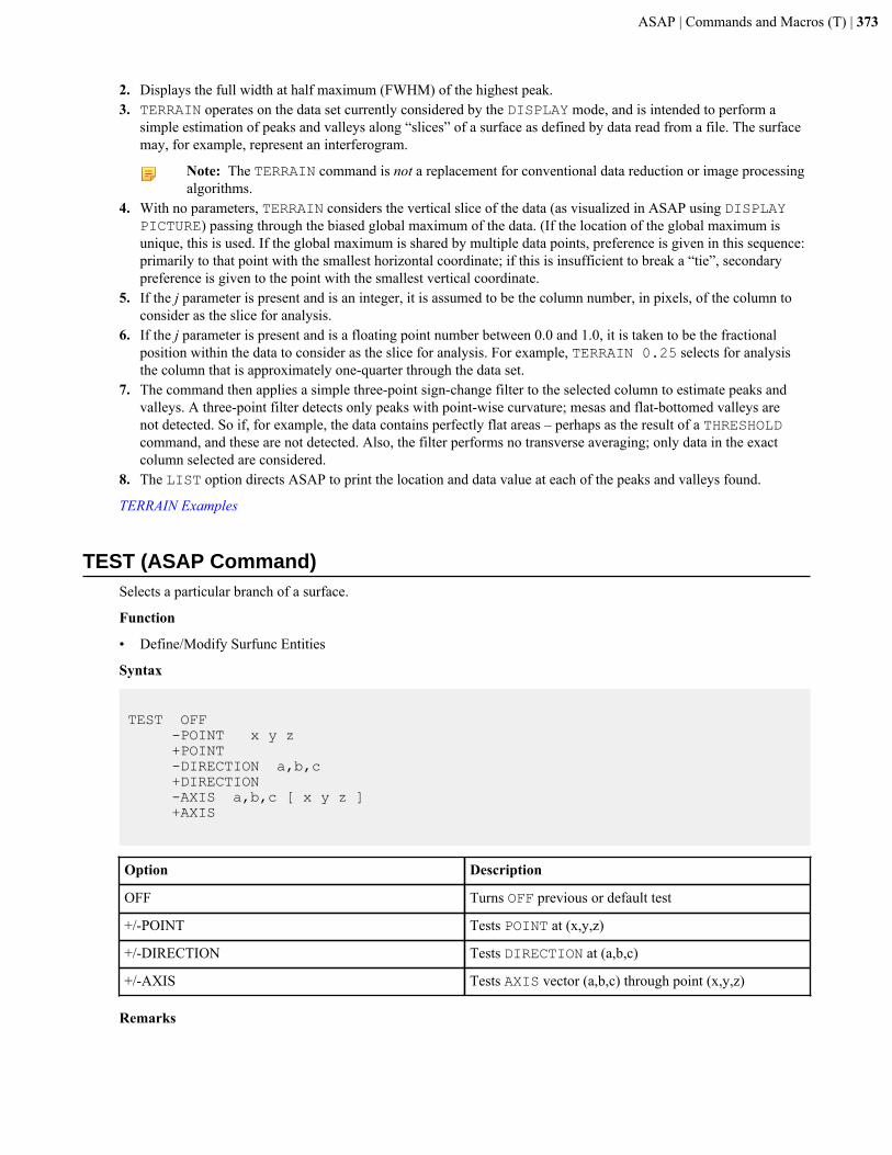
ASAP | Commands and Macros (T) | 373
2. Displays the full width at half maximum (FWHM) of the highest peak.3. TERRAIN operates on the data set currently considered by the DISPLAY mode, and is intended to perform a
simple estimation of peaks and valleys along “slices” of a surface as defined by data read from a file. The surfacemay, for example, represent an interferogram.
Note: The TERRAIN command is not a replacement for conventional data reduction or image processingalgorithms.
4. With no parameters, TERRAIN considers the vertical slice of the data (as visualized in ASAP using DISPLAYPICTURE) passing through the biased global maximum of the data. (If the location of the global maximum isunique, this is used. If the global maximum is shared by multiple data points, preference is given in this sequence:primarily to that point with the smallest horizontal coordinate; if this is insufficient to break a “tie”, secondarypreference is given to the point with the smallest vertical coordinate.
5. If the j parameter is present and is an integer, it is assumed to be the column number, in pixels, of the column toconsider as the slice for analysis.
6. If the j parameter is present and is a floating point number between 0.0 and 1.0, it is taken to be the fractionalposition within the data to consider as the slice for analysis. For example, TERRAIN 0.25 selects for analysisthe column that is approximately one-quarter through the data set.
7. The command then applies a simple three-point sign-change filter to the selected column to estimate peaks andvalleys. A three-point filter detects only peaks with point-wise curvature; mesas and flat-bottomed valleys arenot detected. So if, for example, the data contains perfectly flat areas – perhaps as the result of a THRESHOLDcommand, and these are not detected. Also, the filter performs no transverse averaging; only data in the exactcolumn selected are considered.
8. The LIST option directs ASAP to print the location and data value at each of the peaks and valleys found.
TERRAIN Examples
TEST (ASAP Command)Selects a particular branch of a surface.
Function
• Define/Modify Surfunc Entities
Syntax
TEST OFF -POINT x y z +POINT -DIRECTION a,b,c +DIRECTION -AXIS a,b,c [ x y z ] +AXIS
Option Description
OFF Turns OFF previous or default test
+/-POINT Tests POINT at (x,y,z)
+/-DIRECTION Tests DIRECTION at (a,b,c)
+/-AXIS Tests AXIS vector (a,b,c) through point (x,y,z)
Remarks

ASAP | Commands and Macros (T) | 374
1. If a surface of order two or greater has multiple branches, usually only one of them is of interest. This problem isequivalent to the alternate-surface intersection problem that is seen in conventional optical design software. UseTEST to select a given branch relative to a test point or direction.
2. TEST initiates the following action: at each intersection with the surface, ASAP calculates the dot product ofthe DIRECTION or the vector from the POINT to the intersection and the gradient of the SURFACE at thepoint of intersection. The AXIS syntax is useful for surfaces of cylindrical symmetry. ASAP computes a vectorperpendicular to the AXIS relative to a point on the surface. In all cases, the intersection is valid only if the resulthas the indicated sign. Only one entry (OFF/POINT/DIRECTION/AXIS) can be used at a time with TEST.
3. Certain commands (OPTICAL, AXICONIC and others) internally generate a test in an attempt to select theappropriate branch. In the event the logic fails, it is usually necessary to issue a new TEST command to get thedesired surface.
TEST Examples
TEXT (ASAP Command Argument)Prints text annotation within the graphics window.
Function
• Standard Plot Options
Syntax
... TEXTx y [ z ] x' y' [ z' ] x" y" [ z" ] [ k ] 'string':
Option Description
x y [ z ] Starting point
x' y' [ z' ] Character spacing vector
x" y" [ z" ] Character height vector
k Color number (1-26)
'string' Text annotation
Remarks
1. ASAP command arguments are optional and must follow a command.2. Draws text of color k (default 1) on 2D and 3D plots. See the topic “COLORS (Command Argument)" for a list of
colors.3. The number of entries determines whether the starting point, character-spacing vector and character-height vector
are in 2D plot units or 3D system units as follows:
• If the number of entries is seven or less, ASAP assumes 2D only, paper coordinates (0-10, 0-7.5).• If the number of entries is eight or more, ASAP assumes 3D (and 2D projection) system coordinates.
4. With 2D coordinates, the plot window is 10 inches wide (horizontal or x direction) by 7.5 inches high (vertical ory direction). Especially useful for placing text relative to the plotting window. Using 2D paper coordinates to placetext next to a system OBJECT can be difficult, since the location of plotted OBJECTs in the window changesaccording to the setting of the WINDOW command.
5. The starting point and vector entries for placing text on 3D and 2D projection plots are expressed in global systemcoordinates. Remember that the WINDOW setting determines the apparent size of the text on a given plot, so sizethe text in proportion to the size of the OBJECTs that you want to view in the plot WINDOW.
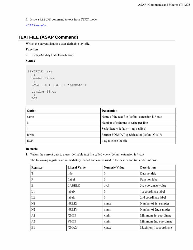
ASAP | Commands and Macros (T) | 375
6. Issue a RETURN command to exit from TEXT mode.
TEXT Examples
TEXTFILE (ASAP Command)Writes the current data to a user-definable text file.
Function
• Display/Modify Data Distributions
Syntax
TEXTFILE name : header lines : DATA [ k ] [ s ] [ 'format' ] : trailer lines : EOF
Option Description
name Name of the text file (default extension is *.txt)
k Number of columns to write per line
s Scale factor (default=1; no scaling)
format Fortran FORMAT specification (default G15.7)
EOF Flag to close the file
Remarks
1. Writes the current data to a user-definable text file called name (default extension is *.txt).
The following registers are immediately loaded and can be used in the header and trailer definitions:
Register Literal Value Numeric Value Description
T title 0 Data set title
F flabel 0 Function label
Z LABELZ zval 3rd coordinate value
L1 labelx 0 1st coordinate label
L2 labely 0 2nd coordinate label
N1 NUMX numx Number of 1st samples
N2 NUMY numy Number of 2nd samples
A1 XMIN xmin Minimum 1st coordinate
A2 YMIN ymin Minimum 2nd coordinate
B1 XMAX xmax Maximum 1st coordinate
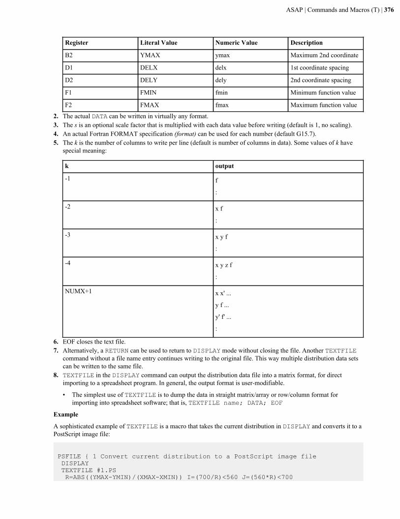
ASAP | Commands and Macros (T) | 376
Register Literal Value Numeric Value Description
B2 YMAX ymax Maximum 2nd coordinate
D1 DELX delx 1st coordinate spacing
D2 DELY dely 2nd coordinate spacing
F1 FMIN fmin Minimum function value
F2 FMAX fmax Maximum function value
2. The actual DATA can be written in virtually any format.3. The s is an optional scale factor that is multiplied with each data value before writing (default is 1, no scaling).4. An actual Fortran FORMAT specification (format) can be used for each number (default G15.7).5. The k is the number of columns to write per line (default is number of columns in data). Some values of k have
special meaning:
k output
-1 f
:
-2 x f
:
-3 x y f
:
-4 x y z f
:
NUMX+1 x x' ...
y f ...
y' f' ...
:
6. EOF closes the text file.7. Alternatively, a RETURN can be used to return to DISPLAY mode without closing the file. Another TEXTFILE
command without a file name entry continues writing to the original file. This way multiple distribution data setscan be written to the same file.
8. TEXTFILE in the DISPLAY command can output the distribution data file into a matrix format, for directimporting to a spreadsheet program. In general, the output format is user-modifiable.
• The simplest use of TEXTFILE is to dump the data in straight matrix/array or row/column format forimporting into spreadsheet software; that is, TEXTFILE name; DATA; EOF
Example
A sophisticated example of TEXTFILE is a macro that takes the current distribution in DISPLAY and converts it to aPostScript image file:
PSFILE { 1 Convert current distribution to a PostScript image file DISPLAY TEXTFILE #1.PS R=ABS((YMAX-YMIN)/(XMAX-XMIN)) I=(700/R)<560 J=(560*R)<700
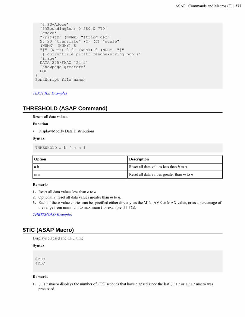
ASAP | Commands and Macros (T) | 377
'%!PS-Adobe' '%%BoundingBox: 0 580 0 770' 'gsave' "/picstr" (NUMX) "string def" 20 20 "translate" (I) (J) "scale" (NUMX) (NUMY) 8 "[" (NUMX) 0 0 -(NUMY) 0 (NUMY) "]" '{ currentfile picstr readhexstring pop }' 'image' DATA 255/FMAX 'Z2.2' 'showpage grestore' EOF}PostScript file name>
TEXTFILE Examples
THRESHOLD (ASAP Command)Resets all data values.
Function
• Display/Modify Data Distributions
Syntax
THRESHOLD a b [ m n ]
Option Description
a b Reset all data values less than b to a
m n Reset all data values greater than m to n
Remarks
1. Reset all data values less than b to a.2. Optionally, reset all data values greater than m to n.3. Each of these value entries can be specified either directly, as the MIN, AVE or MAX value, or as a percentage of
the range from minimum to maximum (for example, 33.3%).
THRESHOLD Examples
$TIC (ASAP Macro)Displays elapsed and CPU time.
Syntax
$TIC&TIC
Remarks
1. $TIC macro displays the number of CPU seconds that have elapsed since the last $TIC or &TIC macro wasprocessed.
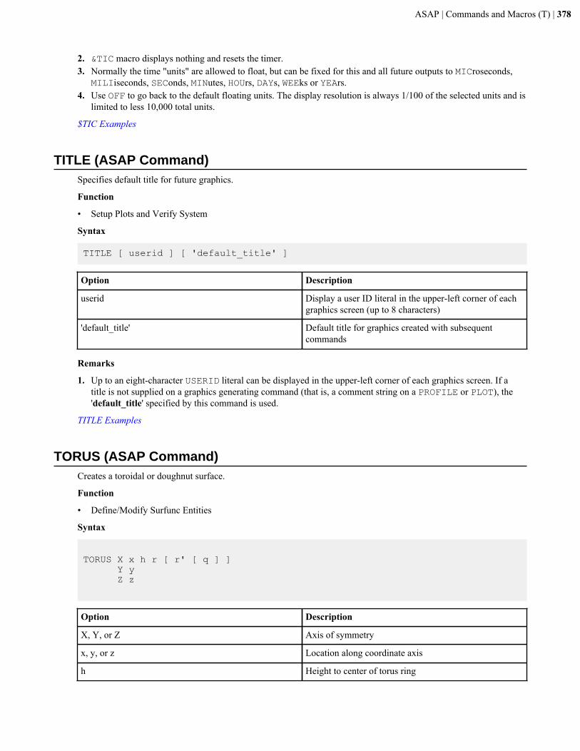
ASAP | Commands and Macros (T) | 378
2. &TIC macro displays nothing and resets the timer.3. Normally the time "units" are allowed to float, but can be fixed for this and all future outputs to MICroseconds,
MILIiseconds, SEConds, MINutes, HOUrs, DAYs, WEEks or YEArs.4. Use OFF to go back to the default floating units. The display resolution is always 1/100 of the selected units and is
limited to less 10,000 total units.
$TIC Examples
TITLE (ASAP Command)Specifies default title for future graphics.
Function
• Setup Plots and Verify System
Syntax
TITLE [ userid ] [ 'default_title' ]
Option Description
userid Display a user ID literal in the upper-left corner of eachgraphics screen (up to 8 characters)
'default_title' Default title for graphics created with subsequentcommands
Remarks
1. Up to an eight-character USERID literal can be displayed in the upper-left corner of each graphics screen. If atitle is not supplied on a graphics generating command (that is, a comment string on a PROFILE or PLOT), the'default_title' specified by this command is used.
TITLE Examples
TORUS (ASAP Command)Creates a toroidal or doughnut surface.
Function
• Define/Modify Surfunc Entities
Syntax
TORUS X x h r [ r' [ q ] ] Y y Z z
Option Description
X, Y, or Z Axis of symmetry
x, y, or z Location along coordinate axis
h Height to center of torus ring
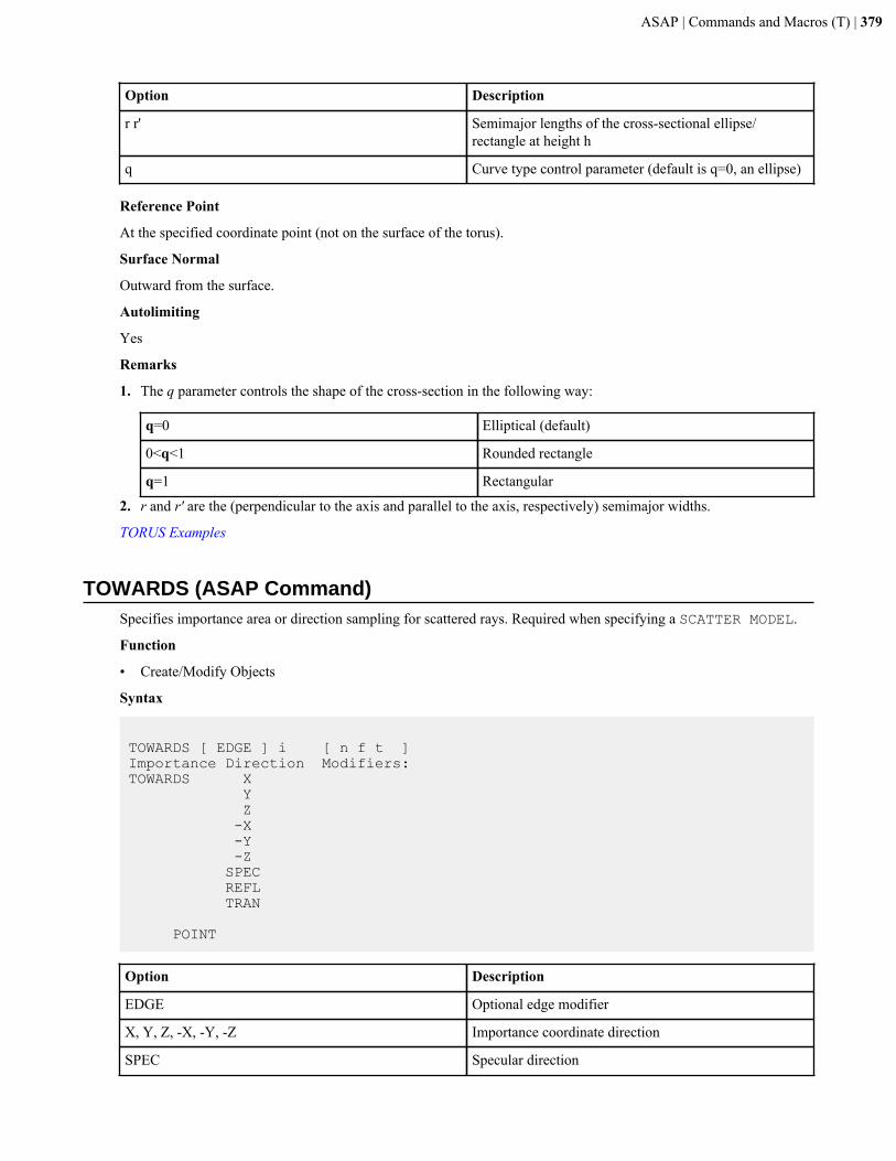
ASAP | Commands and Macros (T) | 379
Option Description
r r' Semimajor lengths of the cross-sectional ellipse/rectangle at height h
q Curve type control parameter (default is q=0, an ellipse)
Reference Point
At the specified coordinate point (not on the surface of the torus).
Surface Normal
Outward from the surface.
Autolimiting
Yes
Remarks
1. The q parameter controls the shape of the cross-section in the following way:
q=0 Elliptical (default)
0<q<1 Rounded rectangle
q=1 Rectangular
2. r and r' are the (perpendicular to the axis and parallel to the axis, respectively) semimajor widths.
TORUS Examples
TOWARDS (ASAP Command)Specifies importance area or direction sampling for scattered rays. Required when specifying a SCATTER MODEL.
Function
• Create/Modify Objects
Syntax
TOWARDS [ EDGE ] i [ n f t ]Importance Direction Modifiers:TOWARDS X Y Z -X -Y -Z SPEC REFL TRAN
POINT
Option Description
EDGE Optional edge modifier
X, Y, Z, -X, -Y, -Z Importance coordinate direction
SPEC Specular direction
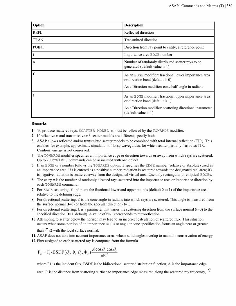
ASAP | Commands and Macros (T) | 380
Option Description
REFL Reflected direction
TRAN Transmitted direction
POINT Direction from ray point to entity, a reference point
i Importance area EDGE number
n Number of randomly distributed scatter rays to begenerated (default value is 1)
f As an EDGE modifier: fractional lower importance areaor direction band (default is 0)
As a Direction modifier: cone half-angle in radians
t As an EDGE modifier: fractional upper importance areaor direction band (default is 1)
As a Direction modifier: scattering directional parameter(default value is 1)
Remarks
1. To produce scattered rays, SCATTER MODEL m must be followed by the TOWARDS modifier.2. If reflective m and transmissive m' scatter models are different, specify both.3. ASAP allows reflected and/or transmitted scatter models to be combined with total internal reflection (TIR). This
enables, for example, approximate simulation of lossy waveguides, for which scatter partially frustrates TIR.Caution: energy is not conserved.
4. The TOWARDS modifier specifies an importance edge or direction towards or away from which rays are scattered.Up to 20 TOWARDS commands can be associated with one object.
5. If an EDGE or a number follows the TOWARDS option, i specifies the EDGE number (relative or absolute) used asan importance area. If i is entered as a positive number, radiation is scattered towards the designated real area; if iis negative, radiation is scattered away from the designated virtual area. Use only rectangular or elliptical EDGEs.
6. The entry n is the number of randomly directed rays scattered into the importance area or importance direction byeach TOWARDS command.
7. For EDGE scattering, f and t are the fractional lower and upper bounds (default 0 to 1) of the importance arearelative to the defining edge.
8. For directional scattering, f is the cone angle in radians into which rays are scattered. This angle is measured fromthe surface normal (t=0) or from the specular direction (t=1).
9. For directional scattering, t is a parameter that varies the scattering direction from the surface normal (t=0) to thespecified direction (t=1, default). A value of t=-1 corresponds to retroreflection.
10. Attempting to scatter below the horizon may lead to an incorrect calculation of scattered flux. This situationoccurs when some portion of an importance EDGE or angular cone specification forms an angle near or greater
than /2 with the local surface normal.11. ASAP does not take into account importance areas whose solid angles overlap to maintain conservation of energy.12. Flux assigned to each scattered ray is computed from the formula
where F1 is the incident flux, BSDF is the bidirectional scatter distribution function, A is the importance edge
area, R is the distance from scattering surface to importance edge measured along the scattered ray trajectory,
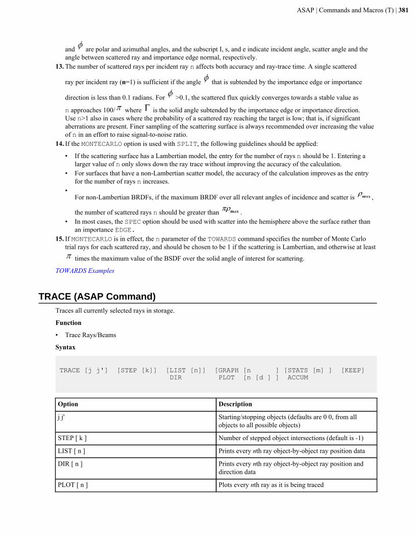
ASAP | Commands and Macros (T) | 381
and are polar and azimuthal angles, and the subscript I, s, and e indicate incident angle, scatter angle and theangle between scattered ray and importance edge normal, respectively.
13. The number of scattered rays per incident ray n affects both accuracy and ray-trace time. A single scattered
ray per incident ray (n=1) is sufficient if the angle that is subtended by the importance edge or importance
direction is less than 0.1 radians. For >0.1, the scattered flux quickly converges towards a stable value as
n approaches 100/ where is the solid angle subtended by the importance edge or importance direction.Use n>1 also in cases where the probability of a scattered ray reaching the target is low; that is, if significantaberrations are present. Finer sampling of the scattering surface is always recommended over increasing the valueof n in an effort to raise signal-to-noise ratio.
14. If the MONTECARLO option is used with SPLIT, the following guidelines should be applied:
• If the scattering surface has a Lambertian model, the entry for the number of rays n should be 1. Entering alarger value of n only slows down the ray trace without improving the accuracy of the calculation.
• For surfaces that have a non-Lambertian scatter model, the accuracy of the calculation improves as the entryfor the number of rays n increases.
•For non-Lambertian BRDFs, if the maximum BRDF over all relevant angles of incidence and scatter is ,
the number of scattered rays n should be greater than .• In most cases, the SPEC option should be used with scatter into the hemisphere above the surface rather than
an importance EDGE.15. If MONTECARLO is in effect, the n parameter of the TOWARDS command specifies the number of Monte Carlo
trial rays for each scattered ray, and should be chosen to be 1 if the scattering is Lambertian, and otherwise at least
times the maximum value of the BSDF over the solid angle of interest for scattering.
TOWARDS Examples
TRACE (ASAP Command)Traces all currently selected rays in storage.
Function
• Trace Rays/Beams
Syntax
TRACE [j j'] [STEP [k]] [LIST [n]] [GRAPH [n ] [STATS [m] ] [KEEP] DIR PLOT [n [d ] ] ACCUM
Option Description
j j' Starting/stopping objects (defaults are 0 0, from allobjects to all possible objects)
STEP [ k ] Number of stepped object intersections (default is -1)
LIST [ n ] Prints every nth ray object-by-object ray position data
DIR [ n ] Prints every nth ray object-by-object ray position anddirection data
PLOT [ n ] Plots every nth ray as it is being traced
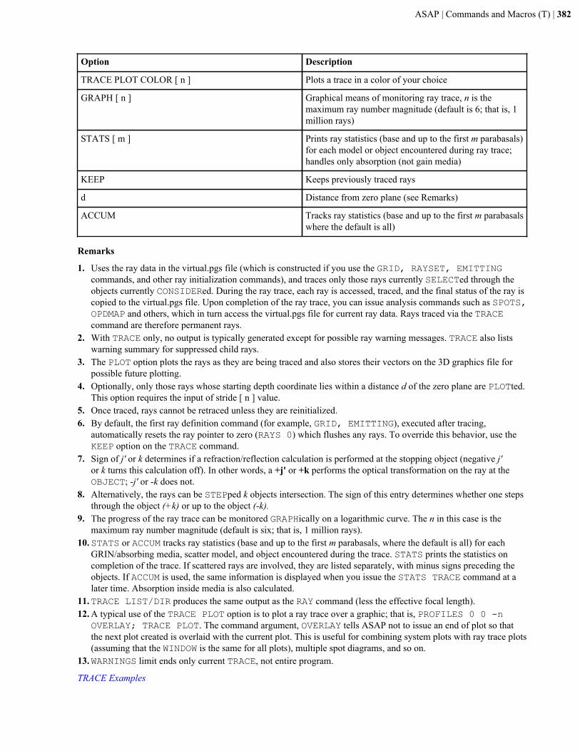
ASAP | Commands and Macros (T) | 382
Option Description
TRACE PLOT COLOR [ n ] Plots a trace in a color of your choice
GRAPH [ n ] Graphical means of monitoring ray trace, n is themaximum ray number magnitude (default is 6; that is, 1million rays)
STATS [ m ] Prints ray statistics (base and up to the first m parabasals)for each model or object encountered during ray trace;handles only absorption (not gain media)
KEEP Keeps previously traced rays
d Distance from zero plane (see Remarks)
ACCUM Tracks ray statistics (base and up to the first m parabasalswhere the default is all)
Remarks
1. Uses the ray data in the virtual.pgs file (which is constructed if you use the GRID, RAYSET, EMITTINGcommands, and other ray initialization commands), and traces only those rays currently SELECTed through theobjects currently CONSIDERed. During the ray trace, each ray is accessed, traced, and the final status of the ray iscopied to the virtual.pgs file. Upon completion of the ray trace, you can issue analysis commands such as SPOTS,OPDMAP and others, which in turn access the virtual.pgs file for current ray data. Rays traced via the TRACEcommand are therefore permanent rays.
2. With TRACE only, no output is typically generated except for possible ray warning messages. TRACE also listswarning summary for suppressed child rays.
3. The PLOT option plots the rays as they are being traced and also stores their vectors on the 3D graphics file forpossible future plotting.
4. Optionally, only those rays whose starting depth coordinate lies within a distance d of the zero plane are PLOTted.This option requires the input of stride [ n ] value.
5. Once traced, rays cannot be retraced unless they are reinitialized.6. By default, the first ray definition command (for example, GRID, EMITTING), executed after tracing,
automatically resets the ray pointer to zero (RAYS 0) which flushes any rays. To override this behavior, use theKEEP option on the TRACE command.
7. Sign of j' or k determines if a refraction/reflection calculation is performed at the stopping object (negative j'or k turns this calculation off). In other words, a +j' or +k performs the optical transformation on the ray at theOBJECT; -j' or -k does not.
8. Alternatively, the rays can be STEPped k objects intersection. The sign of this entry determines whether one stepsthrough the object (+k) or up to the object (-k).
9. The progress of the ray trace can be monitored GRAPHically on a logarithmic curve. The n in this case is themaximum ray number magnitude (default is six; that is, 1 million rays).
10.STATS or ACCUM tracks ray statistics (base and up to the first m parabasals, where the default is all) for eachGRIN/absorbing media, scatter model, and object encountered during the trace. STATS prints the statistics oncompletion of the trace. If scattered rays are involved, they are listed separately, with minus signs preceding theobjects. If ACCUM is used, the same information is displayed when you issue the STATS TRACE command at alater time. Absorption inside media is also calculated.
11.TRACE LIST/DIR produces the same output as the RAY command (less the effective focal length).12. A typical use of the TRACE PLOT option is to plot a ray trace over a graphic; that is, PROFILES 0 0 -n
OVERLAY; TRACE PLOT. The command argument, OVERLAY tells ASAP not to issue an end of plot so thatthe next plot created is overlaid with the current plot. This is useful for combining system plots with ray trace plots(assuming that the WINDOW is the same for all plots), multiple spot diagrams, and so on.
13.WARNINGS limit ends only current TRACE, not entire program.
TRACE Examples
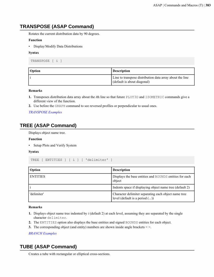
ASAP | Commands and Macros (T) | 383
TRANSPOSE (ASAP Command)Rotates the current distribution data by 90 degrees.
Function
• Display/Modify Data Distributions
Syntax
TRANSPOSE [ i ]
Option Description
i Line to transpose distribution data array about the line(default is about diagonal)
Remarks
1. Transposes distribution data array about the ith line so that future PLOT3D and ISOMETRIC commands give adifferent view of the function.
2. Use before the GRAPH command to see reversed profiles or perpendicular to usual ones.
TRANSPOSE Examples
TREE (ASAP Command)Displays object name tree.
Function
• Setup Plots and Verify System
Syntax
TREE [ ENTITIES ] [ i ] [ 'delimiter' ]
Option Description
ENTITIES Displays the base entities and BOUNDS entities for eachobject
i Indents space if displaying object name tree (default 2)
'delimiter' Character delimiter separating each object name treelevel (default is a period ( . ))
Remarks
1. Displays object name tree indented by i (default 2) at each level, assuming they are separated by the singlecharacter delimiter.
2. The ENTITIES option also displays the base entities and signed BOUNDS entities for each object.3. The corresponding object (and entity) numbers are shown inside angle brackets < >.
BRANCH Examples
TUBE (ASAP Command)Creates a tube with rectangular or elliptical cross-sections.
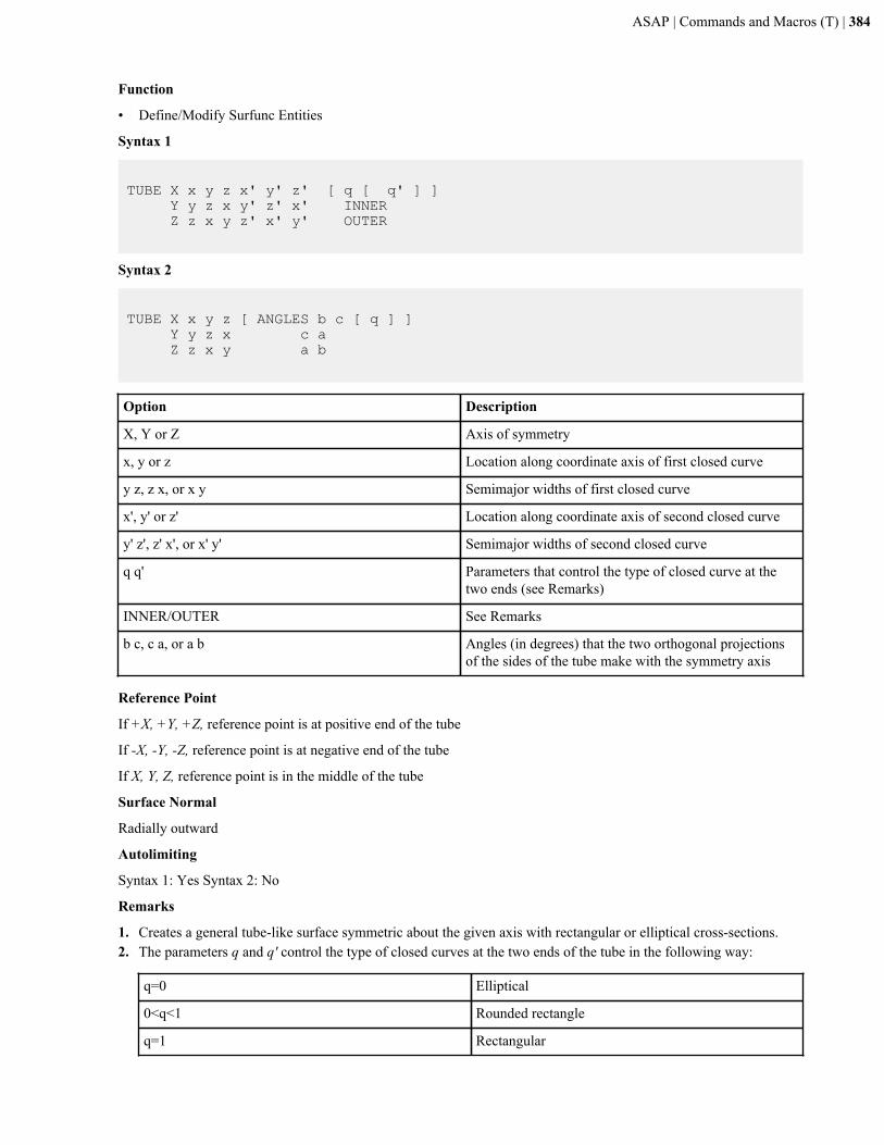
ASAP | Commands and Macros (T) | 384
Function
• Define/Modify Surfunc Entities
Syntax 1
TUBE X x y z x' y' z' [ q [ q' ] ] Y y z x y' z' x' INNER Z z x y z' x' y' OUTER
Syntax 2
TUBE X x y z [ ANGLES b c [ q ] ] Y y z x c a Z z x y a b
Option Description
X, Y or Z Axis of symmetry
x, y or z Location along coordinate axis of first closed curve
y z, z x, or x y Semimajor widths of first closed curve
x', y' or z' Location along coordinate axis of second closed curve
y' z', z' x', or x' y' Semimajor widths of second closed curve
q q' Parameters that control the type of closed curve at thetwo ends (see Remarks)
INNER/OUTER See Remarks
b c, c a, or a b Angles (in degrees) that the two orthogonal projectionsof the sides of the tube make with the symmetry axis
Reference Point
If +X, +Y, +Z, reference point is at positive end of the tube
If -X, -Y, -Z, reference point is at negative end of the tube
If X, Y, Z, reference point is in the middle of the tube
Surface Normal
Radially outward
Autolimiting
Syntax 1: Yes Syntax 2: No
Remarks
1. Creates a general tube-like surface symmetric about the given axis with rectangular or elliptical cross-sections.2. The parameters q and q' control the type of closed curves at the two ends of the tube in the following way:
q=0 Elliptical
0<q<1 Rounded rectangle
q=1 Rectangular
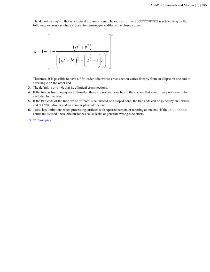
ASAP | Commands and Macros (T) | 385
The default is q=q'=0; that is, elliptical cross-sections. The radius r of the EDGES/CURVES is related to q by thefollowing expression where a,b are the semi-major widths of the closed curve:
Therefore, it is possible to have a fifth-order tube whose cross-section varies linearly from an ellipse on one end toa rectangle on the other end.
3. The default is q=q'=0; that is, elliptical cross-sections.4. If the tube is fourth (q=q') or fifth-order, there are several branches to the surface that may or may not have to be
excluded by the user.5. If the two ends of the tube are of different size, instead of a sloped cone, the two ends can be joined by an INNER
and OUTER cylinder and an annular plane at one end.6. TUBE has limitations when processing surfaces with squared corners or tapering at one end. If the ROUGHNESS
command is used, these circumstances cause leaks or generate wrong-side errors.
TUBE Examples
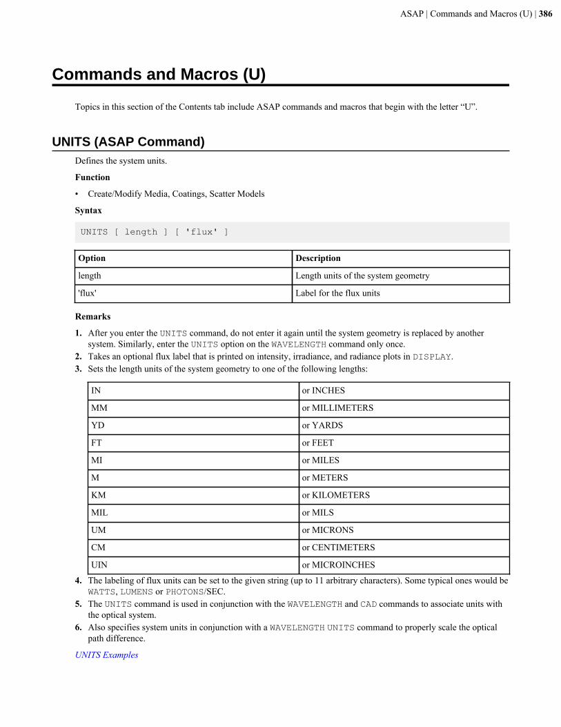
ASAP | Commands and Macros (U) | 386
Commands and Macros (U)
Topics in this section of the Contents tab include ASAP commands and macros that begin with the letter “U”.
UNITS (ASAP Command)Defines the system units.
Function
• Create/Modify Media, Coatings, Scatter Models
Syntax
UNITS [ length ] [ 'flux' ]
Option Description
length Length units of the system geometry
'flux' Label for the flux units
Remarks
1. After you enter the UNITS command, do not enter it again until the system geometry is replaced by anothersystem. Similarly, enter the UNITS option on the WAVELENGTH command only once.
2. Takes an optional flux label that is printed on intensity, irradiance, and radiance plots in DISPLAY.3. Sets the length units of the system geometry to one of the following lengths:
IN or INCHES
MM or MILLIMETERS
YD or YARDS
FT or FEET
MI or MILES
M or METERS
KM or KILOMETERS
MIL or MILS
UM or MICRONS
CM or CENTIMETERS
UIN or MICROINCHES
4. The labeling of flux units can be set to the given string (up to 11 arbitrary characters). Some typical ones would beWATTS, LUMENS or PHOTONS/SEC.
5. The UNITS command is used in conjunction with the WAVELENGTH and CAD commands to associate units withthe optical system.
6. Also specifies system units in conjunction with a WAVELENGTH UNITS command to properly scale the opticalpath difference.
UNITS Examples
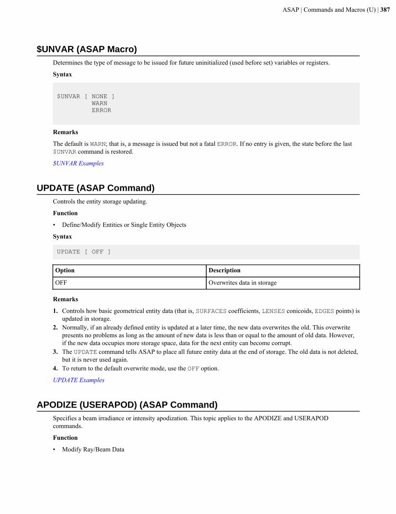
ASAP | Commands and Macros (U) | 387
$UNVAR (ASAP Macro)Determines the type of message to be issued for future uninitialized (used before set) variables or registers.
Syntax
$UNVAR [ NONE ] WARN ERROR
Remarks
The default is WARN; that is, a message is issued but not a fatal ERROR. If no entry is given, the state before the last$UNVAR command is restored.
$UNVAR Examples
UPDATE (ASAP Command)Controls the entity storage updating.
Function
• Define/Modify Entities or Single Entity Objects
Syntax
UPDATE [ OFF ]
Option Description
OFF Overwrites data in storage
Remarks
1. Controls how basic geometrical entity data (that is, SURFACES coefficients, LENSES conicoids, EDGES points) isupdated in storage.
2. Normally, if an already defined entity is updated at a later time, the new data overwrites the old. This overwritepresents no problems as long as the amount of new data is less than or equal to the amount of old data. However,if the new data occupies more storage space, data for the next entity can become corrupt.
3. The UPDATE command tells ASAP to place all future entity data at the end of storage. The old data is not deleted,but it is never used again.
4. To return to the default overwrite mode, use the OFF option.
UPDATE Examples
APODIZE (USERAPOD) (ASAP Command)Specifies a beam irradiance or intensity apodization. This topic applies to the APODIZE and USERAPODcommands.
Function
• Modify Ray/Beam Data
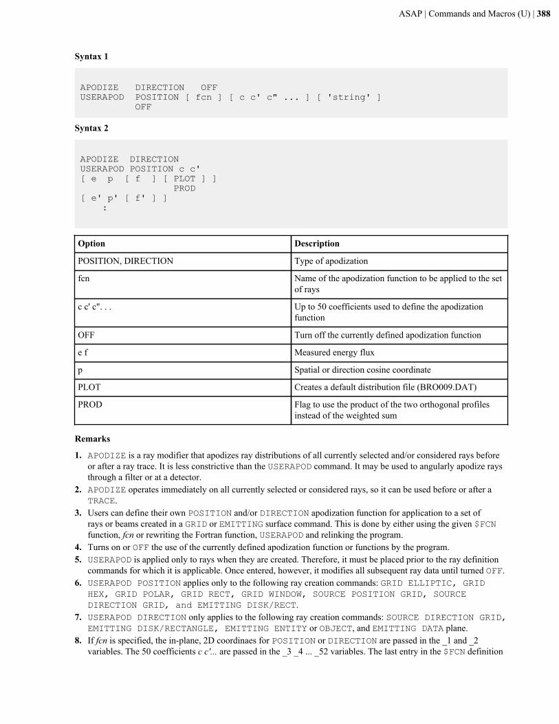
ASAP | Commands and Macros (U) | 388
Syntax 1
APODIZE DIRECTION OFFUSERAPOD POSITION [ fcn ] [ c c' c" ... ] [ 'string' ] OFF
Syntax 2
APODIZE DIRECTIONUSERAPOD POSITION c c'[ e p [ f ] [ PLOT ] ] PROD[ e' p' [ f' ] ] :
Option Description
POSITION, DIRECTION Type of apodization
fcn Name of the apodization function to be applied to the setof rays
c c' c". . . Up to 50 coefficients used to define the apodizationfunction
OFF Turn off the currently defined apodization function
e f Measured energy flux
p Spatial or direction cosine coordinate
PLOT Creates a default distribution file (BRO009.DAT)
PROD Flag to use the product of the two orthogonal profilesinstead of the weighted sum
Remarks
1. APODIZE is a ray modifier that apodizes ray distributions of all currently selected and/or considered rays beforeor after a ray trace. It is less constrictive than the USERAPOD command. It may be used to angularly apodize raysthrough a filter or at a detector.
2. APODIZE operates immediately on all currently selected or considered rays, so it can be used before or after aTRACE.
3. Users can define their own POSITION and/or DIRECTION apodization function for application to a set ofrays or beams created in a GRID or EMITTING surface command. This is done by either using the given $FCNfunction, fcn or rewriting the Fortran function, USERAPOD and relinking the program.
4. Turns on or OFF the use of the currently defined apodization function or functions by the program.5. USERAPOD is applied only to rays when they are created. Therefore, it must be placed prior to the ray definition
commands for which it is applicable. Once entered, however, it modifies all subsequent ray data until turned OFF.6. USERAPOD POSITION applies only to the following ray creation commands: GRID ELLIPTIC, GRID
HEX, GRID POLAR, GRID RECT, GRID WINDOW, SOURCE POSITION GRID, SOURCEDIRECTION GRID, and EMITTING DISK/RECT.
7. USERAPOD DIRECTION only applies to the following ray creation commands: SOURCE DIRECTION GRID,EMITTING DISK/RECTANGLE, EMITTING ENTITY or OBJECT, and EMITTING DATA plane.
8. If fcn is specified, the in-plane, 2D coordinaes for POSITION or DIRECTION are passed in the _1 and _2variables. The 50 coefficients c c'... are passed in the _3 _4 ... _52 variables. The last entry in the $FCN definition
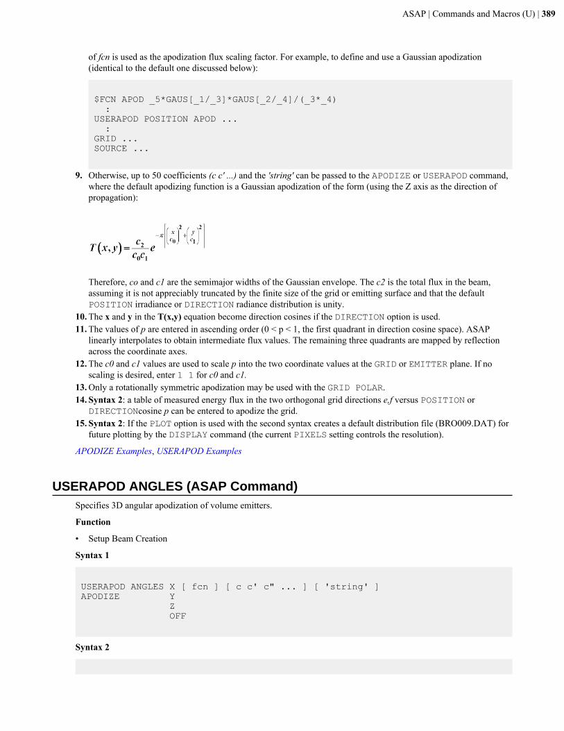
ASAP | Commands and Macros (U) | 389
of fcn is used as the apodization flux scaling factor. For example, to define and use a Gaussian apodization(identical to the default one discussed below):
$FCN APOD _5*GAUS[_1/_3]*GAUS[_2/_4]/(_3*_4) :USERAPOD POSITION APOD ... :GRID ...SOURCE ...
9. Otherwise, up to 50 coefficients (c c' ...) and the 'string' can be passed to the APODIZE or USERAPOD command,where the default apodizing function is a Gaussian apodization of the form (using the Z axis as the direction ofpropagation):
Therefore, co and c1 are the semimajor widths of the Gaussian envelope. The c2 is the total flux in the beam,assuming it is not appreciably truncated by the finite size of the grid or emitting surface and that the defaultPOSITION irradiance or DIRECTION radiance distribution is unity.
10. The x and y in the T(x,y) equation become direction cosines if the DIRECTION option is used.11. The values of p are entered in ascending order (0 < p < 1, the first quadrant in direction cosine space). ASAP
linearly interpolates to obtain intermediate flux values. The remaining three quadrants are mapped by reflectionacross the coordinate axes.
12. The c0 and c1 values are used to scale p into the two coordinate values at the GRID or EMITTER plane. If noscaling is desired, enter 1 1 for c0 and c1.
13. Only a rotationally symmetric apodization may be used with the GRID POLAR.14. Syntax 2: a table of measured energy flux in the two orthogonal grid directions e,f versus POSITION or
DIRECTIONcosine p can be entered to apodize the grid.15. Syntax 2: If the PLOT option is used with the second syntax creates a default distribution file (BRO009.DAT) for
future plotting by the DISPLAY command (the current PIXELS setting controls the resolution).
APODIZE Examples, USERAPOD Examples
USERAPOD ANGLES (ASAP Command)Specifies 3D angular apodization of volume emitters.
Function
• Setup Beam Creation
Syntax 1
USERAPOD ANGLES X [ fcn ] [ c c' c" ... ] [ 'string' ]APODIZE Y Z OFF
Syntax 2
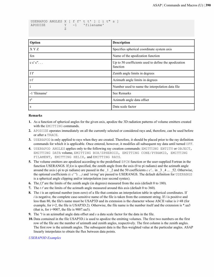
ASAP | Commands and Macros (U) | 390
USERAPOD ANGLES X [ f f' t t' ] [ i t" s ]APODIZE Y -1 'filename' Z
Option Description
X Y Z Specifies spherical coordinate system axis
fcn Name of the apodization function
c c' c". . . Up to 50 coefficients used to define the apodizationfunction
f f' Zenith angle limits in degrees
t t' Azimuth angle limits in degrees
i Number used to name the interpolation data file
-1 'filename' See Remarks
t" Azimuth angle data offset
s Data scale factor
Remarks
1. As a function of spherical angles for the given axis, apodize the 3D radiation patterns of volume emitters createdwith the EMITTING commands.
2. APODIZE operates immediately on all the currently selected or considered rays and, therefore, can be used beforeor after a TRACE.
3. USERAPOD is only applied to rays when they are created. Therefore, it should be placed prior to the ray definitioncommands for which it is applicable. Once entered, however, it modifies all subsequent ray data until turned OFF.
4. USERAPOD ANGLES applies only to the following ray creation commands: EMITTING ENTITY or OBJECT,EMITTING DATA volume, EMITTING BOX/SPHEROID, EMITTING CONE/PYRAMID, EMITTINGFILAMENT, EMITTING HELIX, and EMITTING RAYS.
5. The volume emitters are apodized according to the predefined $FCN function or the user-supplied Fortran in thefunction USERANGS. If fcn is specified, the zenith angle from the axis (0 to pi radians) and the azimuth anglearound the axis (-pi to pi radians) are passed in the _1 _2 and the 50 coefficients c c'... in _3 _4 ... _52. Otherwise,the optional coefficients (c c' "c ...) and 'string' are passed to USERANGS. The default definition for USERANGSis a spherical angle clipping and/or interpolation (see second syntax).
6. The f f' are the limits of the zenith angle (in degrees) measured from the axis (default 0 to 180).7. The t t' are the limits of the azimuth angle measured around this axis (default 0 to 360).8. The i is an optional number (non-zero) of a file that contains an interpolation table in spherical coordinates. If
i is negative, the complete case-sensitive name of the file is taken from the comment string. If i is positive andless than 80, the file's name must be USAP3D and its extension is the character whose ASCII value is i+48 (forexample, for i=2, the file is USAP3D.2). Otherwise, the file name is the number itself and the extension is *.ua3(that is, for i=9007, the file is 9007.ua3).
9. The "t is an azimuthal angle data offset and s a data scale factor for the data in the file.10. Data contained in the file USAP3D.i is used to apodize the emitting volumes. The first two numbers on the first
row of the file are the number of azimuth and zenith angles, respectively. The first column is the zenith angles.The first row is the azimuth angles. The subsequent data is the flux-weighted value at the particular angles. ASAPlinearly interpolates to obtain the flux between data points.
USERAPOD Examples
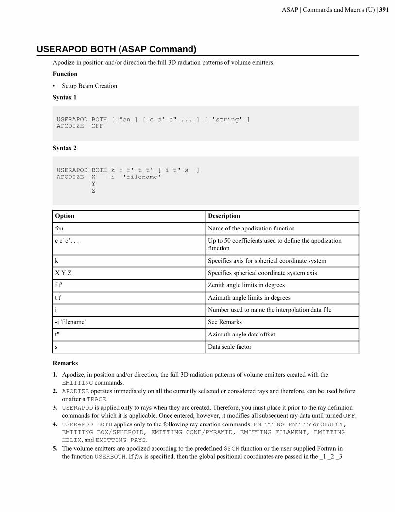
ASAP | Commands and Macros (U) | 391
USERAPOD BOTH (ASAP Command)Apodize in position and/or direction the full 3D radiation patterns of volume emitters.
Function
• Setup Beam Creation
Syntax 1
USERAPOD BOTH [ fcn ] [ c c' c" ... ] [ 'string' ]APODIZE OFF
Syntax 2
USERAPOD BOTH k f f' t t' [ i t" s ]APODIZE X -i 'filename' Y Z
Option Description
fcn Name of the apodization function
c c' c". . . Up to 50 coefficients used to define the apodizationfunction
k Specifies axis for spherical coordinate system
X Y Z Specifies spherical coordinate system axis
f f' Zenith angle limits in degrees
t t' Azimuth angle limits in degrees
i Number used to name the interpolation data file
-i 'filename' See Remarks
t" Azimuth angle data offset
s Data scale factor
Remarks
1. Apodize, in position and/or direction, the full 3D radiation patterns of volume emitters created with theEMITTING commands.
2. APODIZE operates immediately on all the currently selected or considered rays and therefore, can be used beforeor after a TRACE.
3. USERAPOD is applied only to rays when they are created. Therefore, you must place it prior to the ray definitioncommands for which it is applicable. Once entered, however, it modifies all subsequent ray data until turned OFF.
4. USERAPOD BOTH applies only to the following ray creation commands: EMITTING ENTITY or OBJECT,EMITTING BOX/SPHEROID, EMITTING CONE/PYRAMID, EMITTING FILAMENT, EMITTINGHELIX, and EMITTING RAYS.
5. The volume emitters are apodized according to the predefined $FCN function or the user-supplied Fortran inthe function USERBOTH. If fcn is specified, then the global positional coordinates are passed in the _1 _2 _3

ASAP | Commands and Macros (U) | 392
registers, the unit direction vector in _4 _5 _6, and the 50 coefficients c c' ... in _7 _8 ... _56. Otherwise, theoptional coefficients (c c' "c ...) and 'string' are passed to USERBOTH.
6. The default definition for USERBOTH is the same as USERANGS, a spherical angle clipping and/or interpolation(see second syntax).
7. Option k is an axis specification (1=x, 2=y, 3=z) for a spherical coordinate system.8. Option f f' are the limits of the zenith angle (in degrees) measured from this axis (default 0 to 180).9. Option t t' are the limits of the azimuth angle measured around this axis (default 0 to 360).10. Option i is an optional number (non-zero) of a file that contains an interpolation table in spherical coordinates. If i
is negative, the complete case-sensitive name of the file is taken from the comment string. If i is positive and lessthan 80, the name of the file must be USAP3D and its extension is the character whose ASCII value is i+48 (thatis, for i=2, the file is USAP3D.2). Otherwise, the file name is the number itself and the extension is ua3 (that is,for i=9007, the file is 9007.ua3).
11. The "t is an azimuthal angle data offset and s a data scale factor for the data in the file.12. Data contained in the file USAP3D.i is used to apodize the emitting volumes. The first two numbers on the first
row of the file are the numbers of azimuth and zenith angles, respectively. The first column is the zenith angles.The first row is the azimuth angles. The subsequent data is the flux-weighted value at the particular angles. ASAPlinearly interpolates to obtain the flux between data points.
USERAPOD Examples
USERBSDF (ASAP Command)Specifies an isotropic or anisotropic scatter model.
Function
• Create/Modify Media, Coatings, Scatter Models
Syntax - Isotropic-surface Scatter Model (user definable)
USERBSDF [ fcn ] [ SPATIAL ] c c' c" ... [ PLOT [ a a' ... ] ]
Option Description
fcn $FCN (ASAP macro) function
SPATIAL Specifies that the local coordinates of the scatteringlocation are passed to the $FCN function
c c' c" ... Coefficients
PLOT Plots the model in log(b-bo) and angle space
a a' ... User-defined degree specular angles
Syntax - Anisotropic-surface Scatter Model
USERBSDF X [ fcn ] c c' c'' … Y Z :
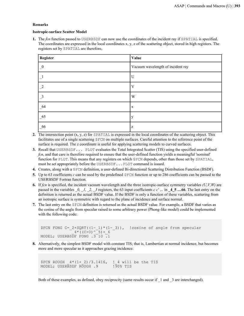
ASAP | Commands and Macros (U) | 393
Remarks
Isotropic-surface Scatter Model
1. The fcn function passed to USERBSDF can now use the coordinates of the incident ray if SPATIAL is specified.The coordinates are expressed in the local coordinates x, y, z of the scattering object, stored in high registers. Theregisters set by SPATIAL are therefore,
Register Value
_0 Vacuum wavelength of incident ray
_1 U
_2 V
_3 W
_64 x
_65 y
_66 z
2. The intersection point (x, y, z) for SPATIAL is expressed in the local coordinates of the scattering object. Thisfacilitates use of a single scattering $FCN on multiple surfaces. Careful attention to the reference point of thesurface is required. The z coordinate is useful for applying scattering models to curved surfaces.
3. Recall that USERBSDF... PLOT evaluates the Total Integrated Scatter (TIS) using the specified user-definedfcn, and that care is therefore required to ensure that the user-defined function yields a meaningful 'nominal'function for PLOT. This means that any registers on which $FCN depends, other than those set by SPATIAL,must be set appropriately before the USERBSDF...PLOT command is issued.
4. Creates, along with a $FCN definition, a user-defined Bi-directional Scattering Distribution Function (BSDF).5. Up to 63 coefficients c can be used by the predefined $FCN function or up to 286 coefficients can be passed to the
USERBSDF Fortran function.6. If fcn is specified, the incident vacuum wavelength and the three isotropic-surface symmetry variables (U,V,W) are
passed in the variables _0, _1, _2, _3 registers, the 63 input coefficients c c' … in _4_5 …66. The last entry on thedefinition is returned as the actual BSDF value. If the BSDF is only a function of these variables, scattering froman isotropic surface is symmetric with regard to the plane of incidence and surface normal.
7. The last entry on the $FCN definition is returned as the actual BSDF value. For example, a BSDF that varies asthe cosine of the angle from specular raised to some arbitrary power (Phong-like model) could be implementedwith the following code:
$FCN FONG C=_2+SQRT((1-_1)*(1-_3)), !cosine of angle from specular _4*((C>0)^_5)+_6MODEL; USERBSDF FONG .3 10 .1
8. Alternatively, the simplest BSDF model with constant TIS; that is, Lambertian at normal incidence, but becomesmore and more specular as it approaches grazing incidence:
$FCN ROUGH _4*(1+_2)/3.1416, !_4 will be the TISMODEL; USERBSDF ROUGH .9 !90% TIS
Both of these examples, as defined, obey reciprocity (same results occur if _1 and _3 are interchanged).
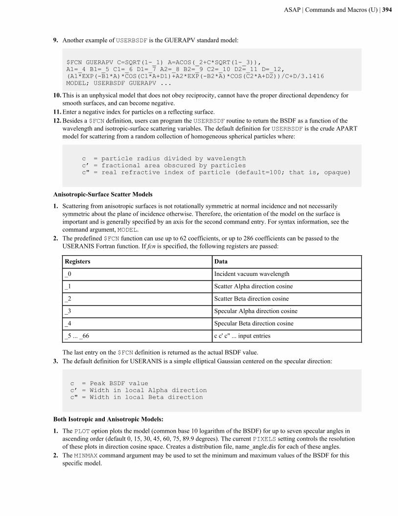
ASAP | Commands and Macros (U) | 394
9. Another example of USERBSDF is the GUERAPV standard model:
$FCN GUERAPV C=SQRT(1-_1) A=ACOS(_2+C*SQRT(1-_3)),A1=_4 B1=_5 C1=_6 D1=_7 A2=_8 B2=_9 C2=_10 D2=_11 D=_12, (A1*EXP(-B1*A)*COS(C1*A+D1)+A2*EXP(-B2*A)*COS(C2*A+D2))/C+D/3.1416MODEL; USERBSDF GUERAPV ...
10. This is an unphysical model that does not obey reciprocity, cannot have the proper directional dependency forsmooth surfaces, and can become negative.
11. Enter a negative index for particles on a reflecting surface.12. Besides a $FCN definition, users can program the USERBSDF routine to return the BSDF as a function of the
wavelength and isotropic-surface scattering variables. The default definition for USERBSDF is the crude APARTmodel for scattering from a random collection of homogeneous spherical particles where:
c = particle radius divided by wavelength c’ = fractional area obscured by particles c" = real refractive index of particle (default=100; that is, opaque)
Anisotropic-Surface Scatter Models
1. Scattering from anisotropic surfaces is not rotationally symmetric at normal incidence and not necessarilysymmetric about the plane of incidence otherwise. Therefore, the orientation of the model on the surface isimportant and is generally specified by an axis for the second command entry. For syntax information, see thecommand argument, MODEL.
2. The predefined $FCN function can use up to 62 coefficients, or up to 286 coefficients can be passed to theUSERANIS Fortran function. If fcn is specified, the following registers are passed:
Registers Data
_0 Incident vacuum wavelength
_1 Scatter Alpha direction cosine
_2 Scatter Beta direction cosine
_3 Specular Alpha direction cosine
_4 Specular Beta direction cosine
_5 ... _66 c c' c" ... input entries
The last entry on the $FCN definition is returned as the actual BSDF value.3. The default definition for USERANIS is a simple elliptical Gaussian centered on the specular direction:
c = Peak BSDF value c’ = Width in local Alpha direction c" = Width in local Beta direction
Both Isotropic and Anisotropic Models:
1. The PLOT option plots the model (common base 10 logarithm of the BSDF) for up to seven specular angles inascending order (default 0, 15, 30, 45, 60, 75, 89.9 degrees). The current PIXELS setting controls the resolutionof these plots in direction cosine space. Creates a distribution file, name_angle.dis for each of these angles.
2. The MINMAX command argument may be used to set the minimum and maximum values of the BSDF for thisspecific model.
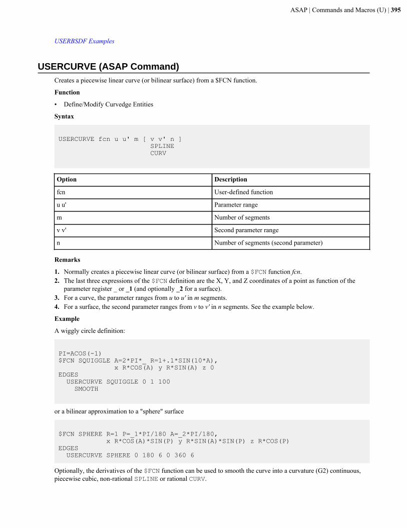
ASAP | Commands and Macros (U) | 395
USERBSDF Examples
USERCURVE (ASAP Command)Creates a piecewise linear curve (or bilinear surface) from a $FCN function.
Function
• Define/Modify Curvedge Entities
Syntax
USERCURVE fcn u u' m [ v v' n ] SPLINE CURV
Option Description
fcn User-defined function
u u' Parameter range
m Number of segments
v v' Second parameter range
n Number of segments (second parameter)
Remarks
1. Normally creates a piecewise linear curve (or bilinear surface) from a $FCN function fcn.2. The last three expressions of the $FCN definition are the X, Y, and Z coordinates of a point as function of the
parameter register _ or _1 (and optionally _2 for a surface).3. For a curve, the parameter ranges from u to u' in m segments.4. For a surface, the second parameter ranges from v to v' in n segments. See the example below.
Example
A wiggly circle definition:
PI=ACOS(-1)$FCN SQUIGGLE A=2*PI*_ R=1+.1*SIN(10*A), x R*COS(A) y R*SIN(A) z 0EDGES USERCURVE SQUIGGLE 0 1 100 SMOOTH
or a bilinear approximation to a "sphere" surface
$FCN SPHERE R=1 P=_1*PI/180 A=_2*PI/180, x R*COS(A)*SIN(P) y R*SIN(A)*SIN(P) z R*COS(P)EDGES USERCURVE SPHERE 0 180 6 0 360 6
Optionally, the derivatives of the $FCN function can be used to smooth the curve into a curvature (G2) continuous,piecewise cubic, non-rational SPLINE or rational CURV.
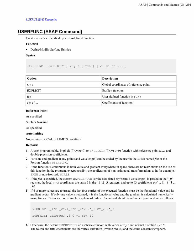
ASAP | Commands and Macros (U) | 396
USERCURVE Examples
USERFUNC (ASAP Command)Creates a surface specified by a user-defined function.
Function
• Define/Modify Surfunc Entities
Syntax
USERFUNC [ EXPLICIT ] x y z [ fcn ] [ c c' c" ... ]
Option Description
x y z Global coordinates of reference point
EXPLICIT Explicit function
fcn User-defined function ($FCN)
c c' c" ... Coefficients of function
Reference Point
As specified
Surface Normal
As specified
Autolimiting
No, requires LOCAL or LIMITS modifiers.
Remarks
1. A user-programmable, implicit (f(x,y,z)=0) or EXPLICIT (f(x,y)-z=0) function with reference point x,y,z anddouble-precision coefficients.
2. Its value and gradient at any point (and wavelength) can be coded by the user in the $FCN named fcn or theFortran function USERFUNC.
3. If the function is continuous in both value and gradient everywhere in space, there are no restrictions on the use ofthis function in the program, except possibly the application of non-orthogonal transformations to it; for example,SKEW or non-isotropic SCALE.
4. If the fcn is specified, the current WAVELENGTH (or the associated ray/beam’s wavelength) is passed in the "_0"register, the local x y z coordinates are passed in the _1 _2 _3 registers, and up to 63 coefficients c c’ ... in _4 _5 ..._66.
5. If 4 or more values are returned, the last four entries of the executed function must be the functional value and itsgradient vector. If only one value is returned, it is the functional value and the gradient is calculated numericallyusing finite-differences. For example, a sphere of radius 10 centered about the reference point is done as follows:
$FCN SPH _1^2+_2^2+_3^2-_4^2 2*_1 2*_2 2*_3 :SURFACE; USERFUNC .5 0 -1 SPH 10
6. Otherwise, the default USERFUNC is an aspheric conicoid with vertex at x,y,z and normal direction c,c’,"c.The fourth and fifth coefficients are the vertex curvature (inverse radius) and the conic constant (0=sphere,
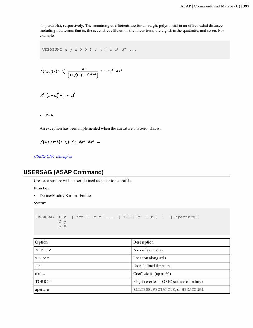
ASAP | Commands and Macros (U) | 397
-1=parabola), respectively. The remaining coefficients are for a straight polynomial in an offset radial distanceincluding odd terms; that is, the seventh coefficient is the linear term, the eighth is the quadratic, and so on. Forexample:
USERFUNC x y z 0 0 1 c k h d d’ d" ...
An exception has been implemented when the curvature c is zero; that is,
USERFUNC Examples
USERSAG (ASAP Command)Creates a surface with a user-defined radial or toric profile.
Function
• Define/Modify Surfunc Entities
Syntax
USERSAG X x [ fcn ] c c' ... [ TORIC r [ k ] ] [ aperture ] Y y Z z
Option Description
X, Y or Z Axis of symmetry
x, y or z Location along axis
fcn User-defined function
c c' ... Coefficients (up to 66)
TORIC r Flag to create a TORIC surface of radius r
aperture ELLIPSE, RECTANGLE, or HEXAGONAL
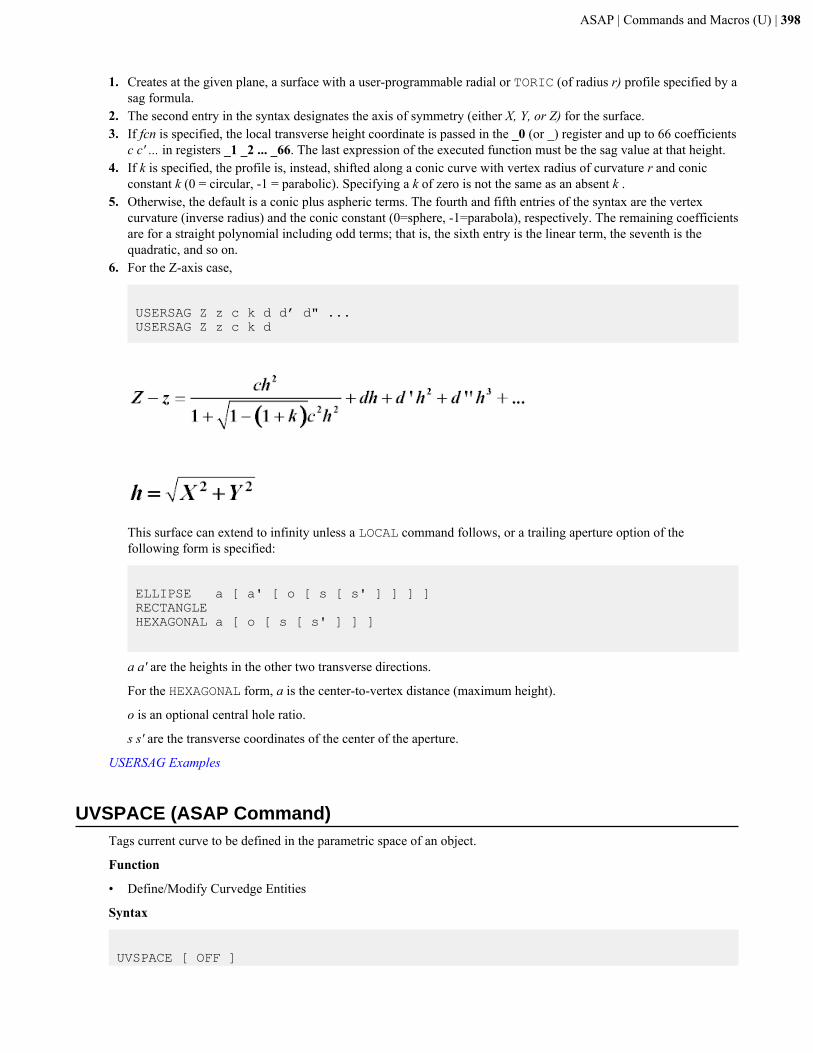
ASAP | Commands and Macros (U) | 398
1. Creates at the given plane, a surface with a user-programmable radial or TORIC (of radius r) profile specified by asag formula.
2. The second entry in the syntax designates the axis of symmetry (either X, Y, or Z) for the surface.3. If fcn is specified, the local transverse height coordinate is passed in the _0 (or _) register and up to 66 coefficients
c c' ... in registers _1 _2 ... _66. The last expression of the executed function must be the sag value at that height.4. If k is specified, the profile is, instead, shifted along a conic curve with vertex radius of curvature r and conic
constant k (0 = circular, -1 = parabolic). Specifying a k of zero is not the same as an absent k .5. Otherwise, the default is a conic plus aspheric terms. The fourth and fifth entries of the syntax are the vertex
curvature (inverse radius) and the conic constant (0=sphere, -1=parabola), respectively. The remaining coefficientsare for a straight polynomial including odd terms; that is, the sixth entry is the linear term, the seventh is thequadratic, and so on.
6. For the Z-axis case,
USERSAG Z z c k d d’ d" ... USERSAG Z z c k d
This surface can extend to infinity unless a LOCAL command follows, or a trailing aperture option of thefollowing form is specified:
ELLIPSE a [ a' [ o [ s [ s' ] ] ] ]RECTANGLEHEXAGONAL a [ o [ s [ s' ] ] ]
a a' are the heights in the other two transverse directions.
For the HEXAGONAL form, a is the center-to-vertex distance (maximum height).
o is an optional central hole ratio.
s s' are the transverse coordinates of the center of the aperture.
USERSAG Examples
UVSPACE (ASAP Command)Tags current curve to be defined in the parametric space of an object.
Function
• Define/Modify Curvedge Entities
Syntax
UVSPACE [ OFF ]
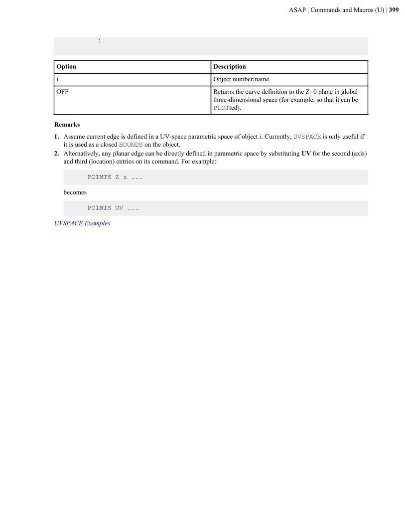
ASAP | Commands and Macros (U) | 399
i
Option Description
i Object number/name
OFF Returns the curve definition to the Z=0 plane in globalthree-dimensional space (for example, so that it can bePLOTted).
Remarks
1. Assume current edge is defined in a UV-space parametric space of object i. Currently, UVSPACE is only useful ifit is used as a closed BOUNDS on the object.
2. Alternatively, any planar edge can be directly defined in parametric space by substituting UV for the second (axis)and third (location) entries on its command. For example:
POINTS Z z ...
becomes
POINTS UV ...
UVSPACE Examples
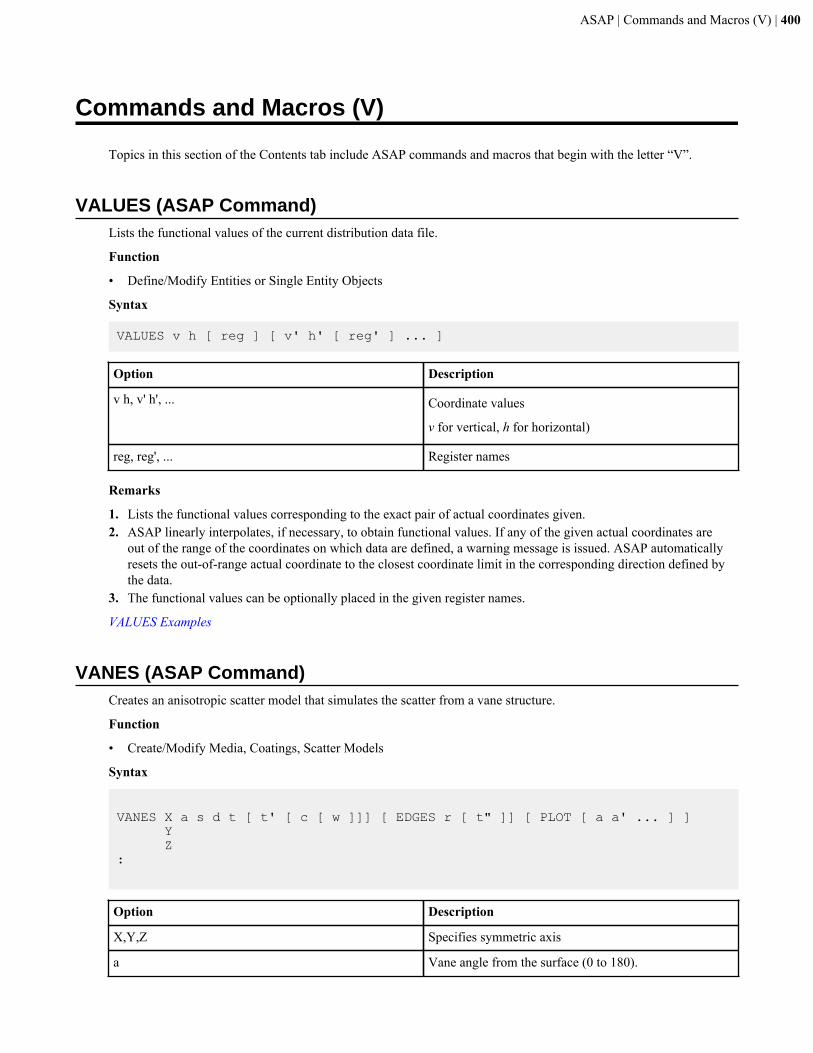
ASAP | Commands and Macros (V) | 400
Commands and Macros (V)
Topics in this section of the Contents tab include ASAP commands and macros that begin with the letter “V”.
VALUES (ASAP Command)Lists the functional values of the current distribution data file.
Function
• Define/Modify Entities or Single Entity Objects
Syntax
VALUES v h [ reg ] [ v' h' [ reg' ] ... ]
Option Description
v h, v' h', ... Coordinate values
v for vertical, h for horizontal)
reg, reg', ... Register names
Remarks
1. Lists the functional values corresponding to the exact pair of actual coordinates given.2. ASAP linearly interpolates, if necessary, to obtain functional values. If any of the given actual coordinates are
out of the range of the coordinates on which data are defined, a warning message is issued. ASAP automaticallyresets the out-of-range actual coordinate to the closest coordinate limit in the corresponding direction defined bythe data.
3. The functional values can be optionally placed in the given register names.
VALUES Examples
VANES (ASAP Command)Creates an anisotropic scatter model that simulates the scatter from a vane structure.
Function
• Create/Modify Media, Coatings, Scatter Models
Syntax
VANES X a s d t [ t' [ c [ w ]]] [ EDGES r [ t" ]] [ PLOT [ a a' ... ] ] Y Z:
Option Description
X,Y,Z Specifies symmetric axis
a Vane angle from the surface (0 to 180).
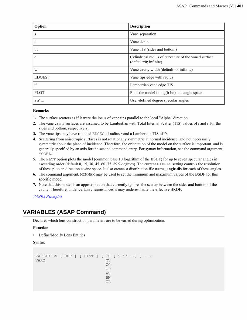
ASAP | Commands and Macros (V) | 401
Option Description
s Vane separation
d Vane depth
t t' Vane TIS (sides and bottom)
c Cylindrical radius of curvature of the vaned surface(default=0; infinite)
w Vane cavity width (default=0; infinite)
EDGES r Vane tips edge with radius
t" Lambertian vane edge TIS
PLOT Plots the model in log(b-bo) and angle space
a a' ... User-defined degree specular angles
Remarks
1. The surface scatters as if it were the locus of vane tips parallel to the local "Alpha" direction.2. The vane cavity surfaces are assumed to be Lambertian with Total Internal Scatter (TIS) values of t and t' for the
sides and bottom, respectively.3. The vane tips may have rounded EDGES of radius r and a Lambertian TIS of "t.4. Scattering from anisotropic surfaces is not rotationally symmetric at normal incidence, and not necessarily
symmetric about the plane of incidence. Therefore, the orientation of the model on the surface is important, and isgenerally specified by an axis for the second command entry. For syntax information, see the command argument,MODEL.
5. The PLOT option plots the model (common base 10 logarithm of the BSDF) for up to seven specular angles inascending order (default 0, 15, 30, 45, 60, 75, 89.9 degrees). The current PIXELS setting controls the resolutionof these plots in direction cosine space. It also creates a distribution file name_angle.dis for each of these angles.
6. The command argument, MINMAX may be used to set the minimum and maximum values of the BSDF for thisspecific model.
7. Note that this model is an approximation that currently ignores the scatter between the sides and bottom of thecavity. Therefore, under certain circumstances it may underestimate the effective BRDF.
VANES Examples
VARIABLES (ASAP Command)Declares which lens construction parameters are to be varied during optimization.
Function
• Define/Modify Lens Entities
Syntax
VARIABLES [ OFF ] [ LIST ] [ TH [ i i'...] ] ...VARY CV CC CP AS BN GL
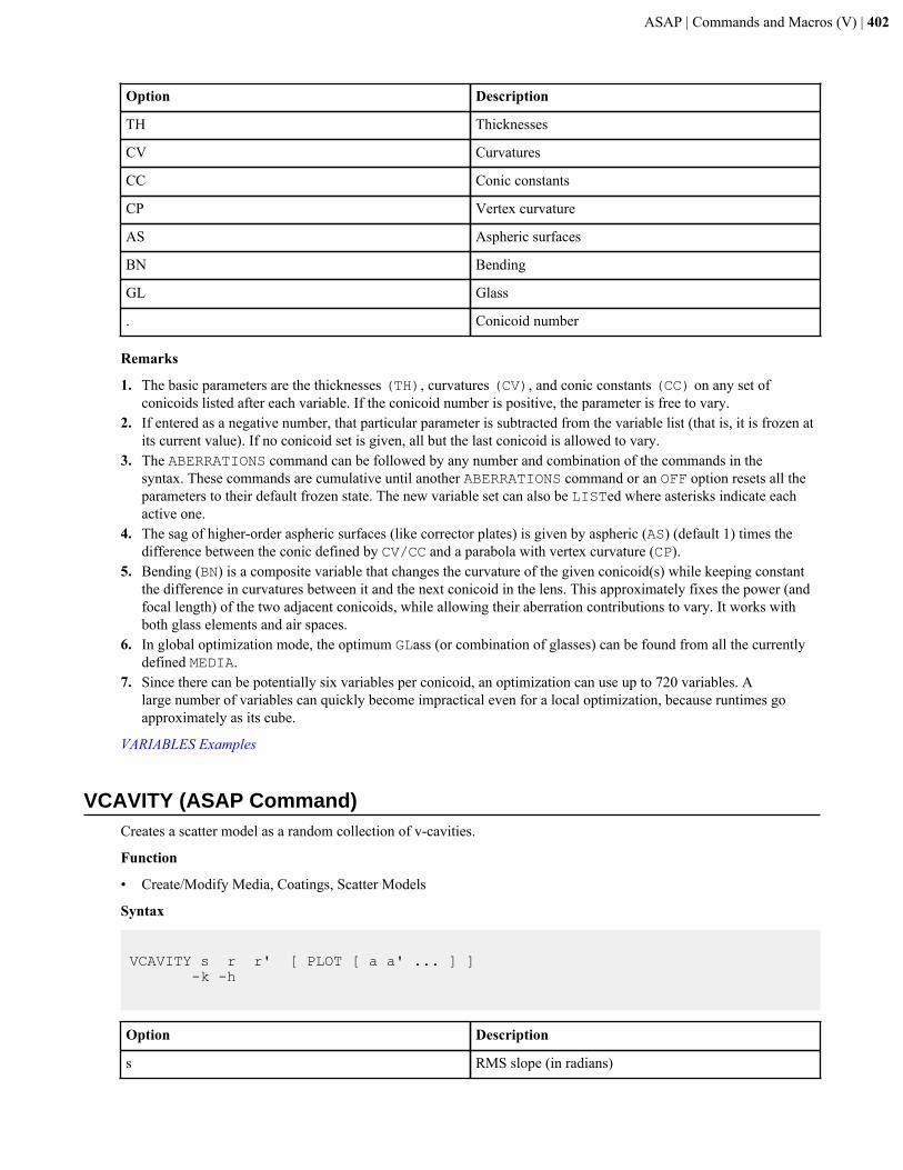
ASAP | Commands and Macros (V) | 402
Option Description
TH Thicknesses
CV Curvatures
CC Conic constants
CP Vertex curvature
AS Aspheric surfaces
BN Bending
GL Glass
. Conicoid number
Remarks
1. The basic parameters are the thicknesses (TH), curvatures (CV), and conic constants (CC) on any set ofconicoids listed after each variable. If the conicoid number is positive, the parameter is free to vary.
2. If entered as a negative number, that particular parameter is subtracted from the variable list (that is, it is frozen atits current value). If no conicoid set is given, all but the last conicoid is allowed to vary.
3. The ABERRATIONS command can be followed by any number and combination of the commands in thesyntax. These commands are cumulative until another ABERRATIONS command or an OFF option resets all theparameters to their default frozen state. The new variable set can also be LISTed where asterisks indicate eachactive one.
4. The sag of higher-order aspheric surfaces (like corrector plates) is given by aspheric (AS) (default 1) times thedifference between the conic defined by CV/CC and a parabola with vertex curvature (CP).
5. Bending (BN) is a composite variable that changes the curvature of the given conicoid(s) while keeping constantthe difference in curvatures between it and the next conicoid in the lens. This approximately fixes the power (andfocal length) of the two adjacent conicoids, while allowing their aberration contributions to vary. It works withboth glass elements and air spaces.
6. In global optimization mode, the optimum GLass (or combination of glasses) can be found from all the currentlydefined MEDIA.
7. Since there can be potentially six variables per conicoid, an optimization can use up to 720 variables. Alarge number of variables can quickly become impractical even for a local optimization, because runtimes goapproximately as its cube.
VARIABLES Examples
VCAVITY (ASAP Command)Creates a scatter model as a random collection of v-cavities.
Function
• Create/Modify Media, Coatings, Scatter Models
Syntax
VCAVITY s r r' [ PLOT [ a a' ... ] ] -k -h
Option Description
s RMS slope (in radians)
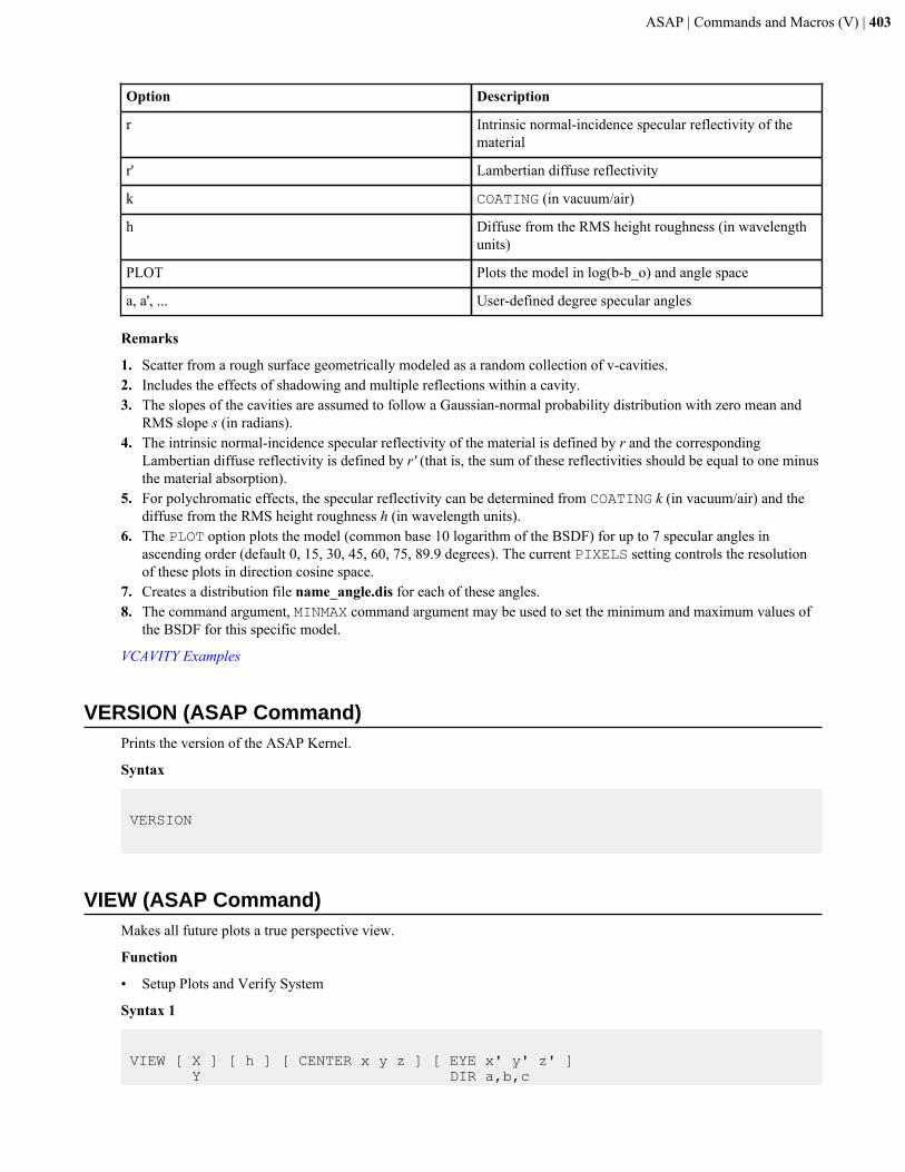
ASAP | Commands and Macros (V) | 403
Option Description
r Intrinsic normal-incidence specular reflectivity of thematerial
r' Lambertian diffuse reflectivity
k COATING (in vacuum/air)
h Diffuse from the RMS height roughness (in wavelengthunits)
PLOT Plots the model in log(b-b_o) and angle space
a, a', ... User-defined degree specular angles
Remarks
1. Scatter from a rough surface geometrically modeled as a random collection of v-cavities.2. Includes the effects of shadowing and multiple reflections within a cavity.3. The slopes of the cavities are assumed to follow a Gaussian-normal probability distribution with zero mean and
RMS slope s (in radians).4. The intrinsic normal-incidence specular reflectivity of the material is defined by r and the corresponding
Lambertian diffuse reflectivity is defined by r' (that is, the sum of these reflectivities should be equal to one minusthe material absorption).
5. For polychromatic effects, the specular reflectivity can be determined from COATING k (in vacuum/air) and thediffuse from the RMS height roughness h (in wavelength units).
6. The PLOT option plots the model (common base 10 logarithm of the BSDF) for up to 7 specular angles inascending order (default 0, 15, 30, 45, 60, 75, 89.9 degrees). The current PIXELS setting controls the resolutionof these plots in direction cosine space.
7. Creates a distribution file name_angle.dis for each of these angles.8. The command argument, MINMAX command argument may be used to set the minimum and maximum values of
the BSDF for this specific model.
VCAVITY Examples
VERSION (ASAP Command)Prints the version of the ASAP Kernel.
Syntax
VERSION
VIEW (ASAP Command)Makes all future plots a true perspective view.
Function
• Setup Plots and Verify System
Syntax 1
VIEW [ X ] [ h ] [ CENTER x y z ] [ EYE x' y' z' ] Y DIR a,b,c
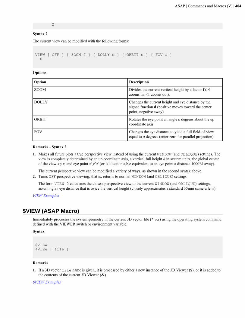
ASAP | Commands and Macros (V) | 404
Z
Syntax 2
The current view can be modified with the following forms:
VIEW [ OFF ] [ ZOOM f ] [ DOLLY d ] [ ORBIT o ] [ FOV a ] 0
Options
Option Description
ZOOM Divides the current vertical height by a factor f (>1zooms in, <1 zooms out).
DOLLY Changes the current height and eye distance by thesigned fraction d (positive moves toward the centerpoint, negative away).
ORBIT Rotates the eye point an angle o degrees about the upcoordinate axis.
FOV Changes the eye distance to yield a full field-of-viewequal to a degrees (enter zero for parallel projection).
Remarks - Syntax 2
1. Makes all future plots a true perspective view instead of using the current WINDOW (and OBLIQUE) settings. Theview is completely determined by an up coordinate axis, a vertical full height h in system units, the global centerof the view x y z, and eye point x' y' z' (or DIRection a,b,c equivalent to an eye point a distance 1000*h away).
The current perspective view can be modified a variety of ways, as shown in the second syntax above.2. Turns OFF perspective viewing; that is, returns to normal WINDOW (and OBLIQUE) settings.
The form VIEW 0 calculates the closest perspective view to the current WINDOW (and OBLIQUE) settings,assuming an eye distance that is twice the vertical height (closely approximates a standard 35mm camera lens).
VIEW Examples
$VIEW (ASAP Macro)Immediately processes the system geometry in the current 3D vector file (*.vcr) using the operating system commanddefined with the VIEWER switch or environment variable.
Syntax
$VIEW&VIEW [ file ]
Remarks
1. If a 3D vector file name is given, it is processed by either a new instance of the 3D Viewer ($), or it is added tothe contents of the current 3D Viewer (&).
$VIEW Examples
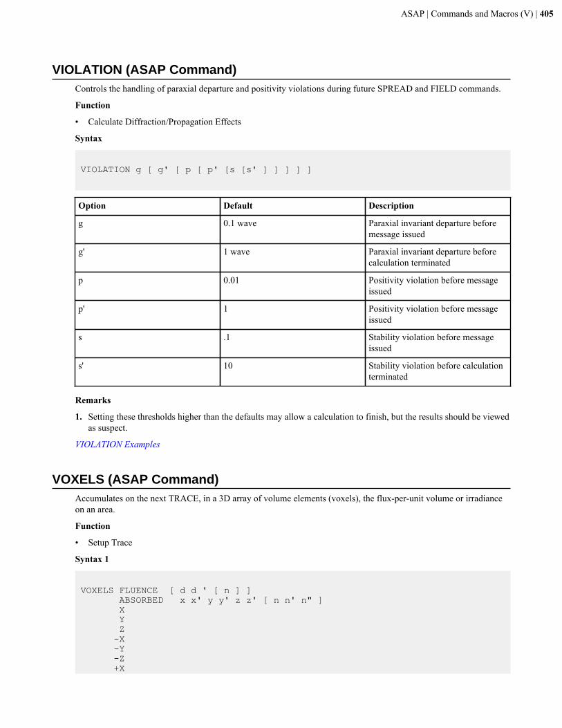
ASAP | Commands and Macros (V) | 405
VIOLATION (ASAP Command)Controls the handling of paraxial departure and positivity violations during future SPREAD and FIELD commands.
Function
• Calculate Diffraction/Propagation Effects
Syntax
VIOLATION g [ g' [ p [ p' [s [s' ] ] ] ] ]
Option Default Description
g 0.1 wave Paraxial invariant departure beforemessage issued
g' 1 wave Paraxial invariant departure beforecalculation terminated
p 0.01 Positivity violation before messageissued
p' 1 Positivity violation before messageissued
s .1 Stability violation before messageissued
s' 10 Stability violation before calculationterminated
Remarks
1. Setting these thresholds higher than the defaults may allow a calculation to finish, but the results should be viewedas suspect.
VIOLATION Examples
VOXELS (ASAP Command)Accumulates on the next TRACE, in a 3D array of volume elements (voxels), the flux-per-unit volume or irradianceon an area.
Function
• Setup Trace
Syntax 1
VOXELS FLUENCE [ d d ' [ n ] ] ABSORBED x x' y y' z z' [ n n' n" ] X Y Z -X -Y -Z +X
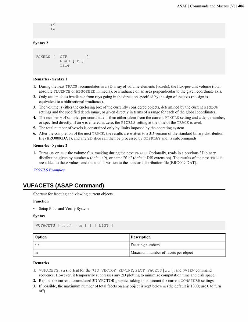
ASAP | Commands and Macros (V) | 406
+Y +Z
Syntax 2
VOXELS [ OFF ] READ [ u ] file
Remarks - Syntax 1
1. During the next TRACE, accumulates in a 3D array of volume elements (voxels), the flux-per-unit volume (totalabsolute FLUENCE or ABSORBED in media), or irradiance on an area perpendicular to the given coordinate axis.
2. Only accumulates irradiance from rays going in the direction specified by the sign of the axis (no sign isequivalent to a bidirectional irradiance).
3. The volume is either the enclosing box of the currently considered objects, determined by the current WINDOWsettings and the specified depth range, or given directly in terms of a range for each of the global coordinates.
4. The number n of samples per coordinate is then either taken from the current PIXELS setting and a depth number,or specified directly. If an n is entered as zero, the PIXELS setting at the time of the TRACE is used.
5. The total number of voxels is constrained only by limits imposed by the operating system.6. After the completion of the next TRACE, the results are written to a 3D version of the standard binary distribution
file (BRO009.DAT), and any 2D slice can then be processed by DISPLAY and its subcommands.
Remarks - Syntax 2
1. Turns ON or OFF the volume flux tracking during the next TRACE. Optionally, reads in a previous 3D binarydistribution given by number u (default 9), or name "file" (default DIS extension). The results of the next TRACEare added to these values, and the total is written to the standard distribution file (BRO009.DAT).
VOXELS Examples
VUFACETS (ASAP Command)Shortcut for faceting and viewing current objects.
Function
• Setup Plots and Verify System
Syntax
VUFACETS [ n n' [ m ] ] [ LIST ]
Option Description
n n' Faceting numbers
m Maximum number of facets per object
Remarks
1. VUFACETS is a shortcut for the $IO VECTOR REWIND, PLOT FACETS [ n n' ], and $VIEW commandsequence. However, it temporarily suppresses any 2D plotting to minimize computation time and disk space.
2. Replots the current accumulated 3D VECTOR graphics taking into account the current CONSIDER settings.3. If possible, the maximum number of total facets on any object is kept below m (the default is 1000; use 0 to turn
off).

ASAP | Commands and Macros (V) | 407
4. Remembers the faceting numbers n n' "m from the previous VUFACETS command (an END command resets themto the default 1).
5. A $VIEW lists the facets in the Command Output window.6. The numbers of facets created for each object can also be LISTed (a $VIEW is not automatically issued in this
case).
VUFACETS Examples

ASAP | Commands and Macros (W) | 408
Commands and Macros (W)
Topics in this section of the Contents tab include ASAP commands and macros that begin with the letter “W”.
$WAIT (ASAP Macro)Causes the program to wait a specified number of seconds (default is 5 seconds) before continuing. An optionalmessage can also be displayed.
Syntax
$WAIT [ s ] [ 'message' ]
$WAIT Examples
WARNINGS (ASAP Command)Controls output of parent ray warning messages.
Function
• Setup Trace
Syntax
WARNINGS [ n ] [ LIST ]
Option Description
n Threshold number of ray warnings
LIST Lists all future warning messages
Remarks
1. Sets a state based on the number of ray warnings.2. If n is zero or greater and more than n ray warnings occur, the raytrace is terminated. The default for n is a
negative number, which means there is no limit on the number of warnings.3. If the LIST option is present, all warning messages are printed during future ray traces.
WARNINGS Examples
WAVELENGTH(S) (ASAP Command)Defines the wavelength(s) for different MEDIA and COATING definitions.
Function
• Create/Modify Media, Coatings, Scatter Models• Setup Beam Creation
Syntax
WAVELENGTH w [ w' w" ... [ name ] ] UNITS u

ASAP | Commands and Macros (W) | 409
Option Description
w w' w" ... Wavelength(s)
name Wavelength units designation
u Multiplier to convert wavelength into system units
Remarks
1. Specifies wavelengths used in media, coatings, and other databases. Multiple wavelengths in either ascending ordescending order must be entered for any MEDIA or COATING commands that have multiple refractive indices orproperties, so as to identify the wavelength for each entry.
2. Sets the wavelength for any future calculations to w (normally in system units).3. WAVELENGTH(S) must precede any ray definitions to properly set up the Gaussian beams used to calculate the
diffracted field.4. To change the wavelength (for setting up rays for tracing, for example), enter the WAVELENGTH(S) command
with the appropriate wavelength. ASAP remembers the wavelength units.5. Enter the UNITS option only once on the WAVELENGTH(S) command.6. WAVELENGTH(S) as measured in vacuum must be entered on WAVELENGTH(S).7. The UNITS option with a scale factor u (default=1) may be used to convert w into system units. The argument u is
almost always a number much less than unity.8. Alternatively, if a basic UNITS command was already issued, any of the following names can be used to calculate
u automatically:
A or ANGSTROMS
NM or NANOMETERS
UM or MICRONS
MM or MILLIMETERS
CM or CENTIMETERS
M or METERS9. Some input parameters have units that are the same as w (see the INTERFACE command), so that it is sometimes
more convenient for these parameters to have different units than the physical system.10. ASAP remembers the units used to define MEDIA; interpolation does not depend on WAVELENGTH units.11. When the WAVELENGTH(S)) command is used with the MEDIA command, up to 40 wavelengths may be
specified for interpolation purposes to determine the refractive index for intermediate wavelengths.12. When the WAVELENGTH(S) command is used with the SPECTRUM command, up to 200 weights, along with
the corresponding wavelengths from the most recent WAVELENGTH(S) command, can be used to create a multi-wavelength spectrum of a source.
13. If a wavelength is not specified for a set of sources, rays and ray paths are plotted in the arbitrary sequence ofcolors from the order in the COLORS command for the sequence of sources.
14. All the rays from one source have the same color, whatever color is appropriate for that source.15. When sources of different wavelengths are created, the colors range from blue to red in a quasi-spectral sense,
corresponding respectively to the wavelengths ranging from shorter to longer.
WAVELENGTHS Examples
WEDGE (ASAP Command)Creates a wedge of glass.
Function
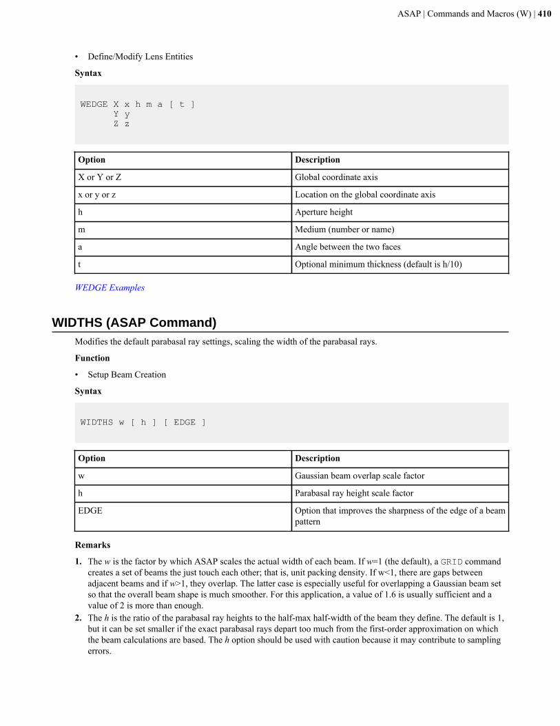
ASAP | Commands and Macros (W) | 410
• Define/Modify Lens Entities
Syntax
WEDGE X x h m a [ t ] Y y Z z
Option Description
X or Y or Z Global coordinate axis
x or y or z Location on the global coordinate axis
h Aperture height
m Medium (number or name)
a Angle between the two faces
t Optional minimum thickness (default is h/10)
WEDGE Examples
WIDTHS (ASAP Command)Modifies the default parabasal ray settings, scaling the width of the parabasal rays.
Function
• Setup Beam Creation
Syntax
WIDTHS w [ h ] [ EDGE ]
Option Description
w Gaussian beam overlap scale factor
h Parabasal ray height scale factor
EDGE Option that improves the sharpness of the edge of a beampattern
Remarks
1. The w is the factor by which ASAP scales the actual width of each beam. If w=1 (the default), a GRID commandcreates a set of beams the just touch each other; that is, unit packing density. If w<1, there are gaps betweenadjacent beams and if w>1, they overlap. The latter case is especially useful for overlapping a Gaussian beam setso that the overall beam shape is much smoother. For this application, a value of 1.6 is usually sufficient and avalue of 2 is more than enough.
2. The h is the ratio of the parabasal ray heights to the half-max half-width of the beam they define. The default is 1,but it can be set smaller if the exact parabasal rays depart too much from the first-order approximation on whichthe beam calculations are based. The h option should be used with caution because it may contribute to samplingerrors.
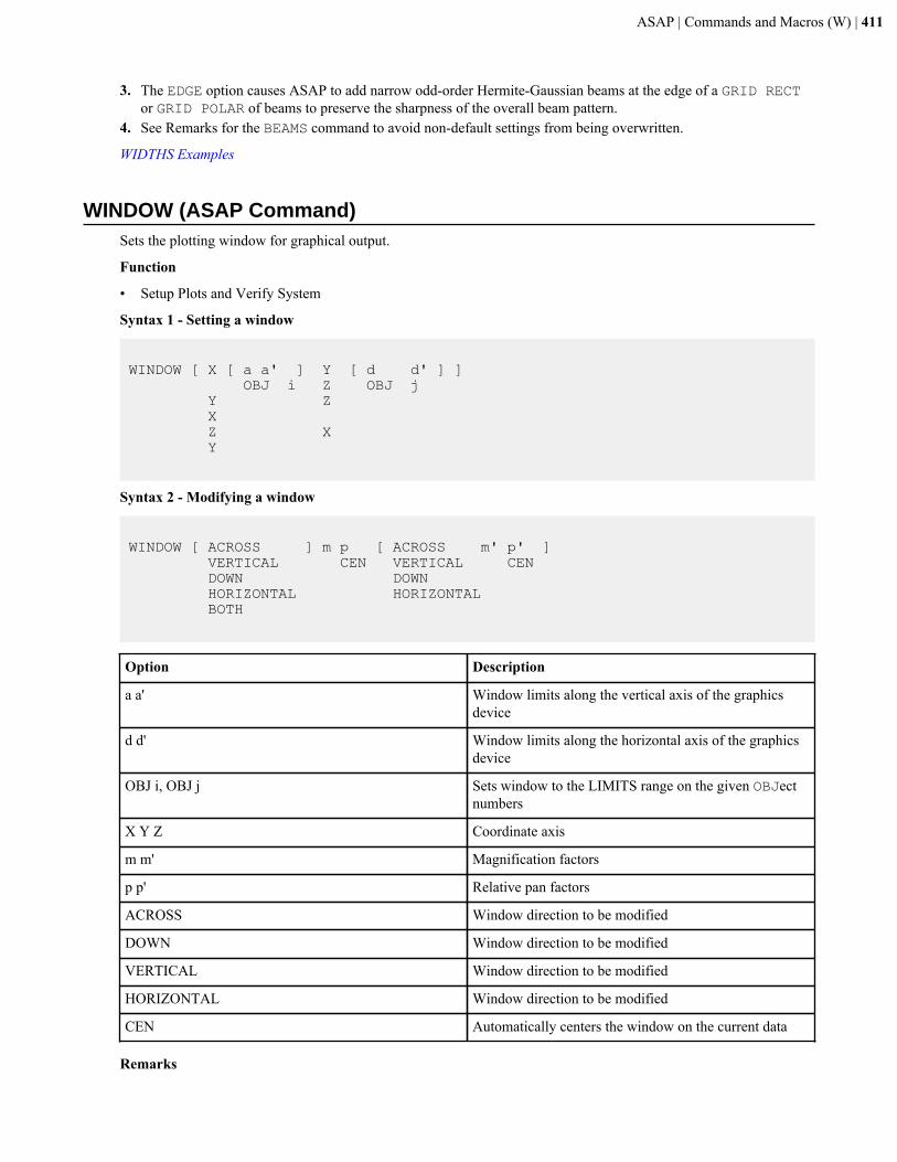
ASAP | Commands and Macros (W) | 411
3. The EDGE option causes ASAP to add narrow odd-order Hermite-Gaussian beams at the edge of a GRID RECTor GRID POLAR of beams to preserve the sharpness of the overall beam pattern.
4. See Remarks for the BEAMS command to avoid non-default settings from being overwritten.
WIDTHS Examples
WINDOW (ASAP Command)Sets the plotting window for graphical output.
Function
• Setup Plots and Verify System
Syntax 1 - Setting a window
WINDOW [ X [ a a' ] Y [ d d' ] ] OBJ i Z OBJ j Y Z X Z X Y
Syntax 2 - Modifying a window
WINDOW [ ACROSS ] m p [ ACROSS m' p' ] VERTICAL CEN VERTICAL CEN DOWN DOWN HORIZONTAL HORIZONTAL BOTH
Option Description
a a' Window limits along the vertical axis of the graphicsdevice
d d' Window limits along the horizontal axis of the graphicsdevice
OBJ i, OBJ j Sets window to the LIMITS range on the given OBJectnumbers
X Y Z Coordinate axis
m m' Magnification factors
p p' Relative pan factors
ACROSS Window direction to be modified
DOWN Window direction to be modified
VERTICAL Window direction to be modified
HORIZONTAL Window direction to be modified
CEN Automatically centers the window on the current data
Remarks
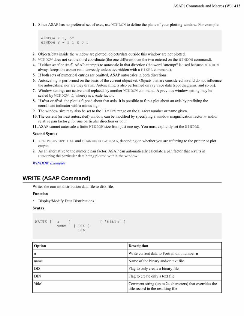
ASAP | Commands and Macros (W) | 412
1. Since ASAP has no preferred set of axes, use WINDOW to define the plane of your plotting window. For example:
WINDOW Y Z, or WINDOW Y - 1 1 Z 0 3
2. Objects/data inside the window are plotted; objects/data outside this window are not plotted.3. WINDOW does not set the third coordinate (the one different than the two entered on the WINDOW command).4. If either a=a' or d=d', ASAP attempts to autoscale in that direction (the word "attempt" is used because WINDOW
always keeps the aspect ratio correctly unless overridden with a PIXEL command).5. If both sets of numerical entries are omitted, ASAP autoscales in both directions.6. Autoscaling is performed on the basis of the current object set. Objects that are considered invalid do not influence
the autoscaling, nor are they drawn. Autoscaling is also performed on ray trace data (spot diagrams, and so on).7. Window settings are active until replaced by another WINDOW command. A previous window setting may be
scaled by WINDOW f, where f is a scale factor.8. If a'<a or d'<d, the plot is flipped about that axis. It is possible to flip a plot about an axis by prefixing the
coordinate indicator with a minus sign.9. The window size may also be set to the LIMITS range on the OBJect number or name given.10. The current (or next autoscaled) window can be modified by specifying a window magnification factor m and/or
relative pan factor p for one particular direction or both.11. ASAP cannot autoscale a finite WINDOW size from just one ray. You must explicitly set the WINDOW.
Second Syntax
1. ACROSS=VERTICAL and DOWN=HORIZONTAL, depending on whether you are referring to the printer or plotoutput.
2. As an alternative to the numeric pan factor, ASAP can automatically calculate a pan factor that results inCENtering the particular data being plotted within the window.
WINDOW Examples
WRITE (ASAP Command)Writes the current distribution data file to disk file.
Function
• Display/Modify Data Distributions
Syntax
WRITE [ u ] [ 'title' ] name [ DIS ] DIN
Option Description
u Write current data to Fortran unit number u
name Name of the binary and/or text file
DIS Flag to only create a binary file
DIN Flag to create only a text file
'title' Comment string (up to 24 characters) that overrides thetitle record in the resulting file

ASAP | Commands and Macros (W) | 413
Remarks
1. Writes the current data to the current file, logical unit number u, binary file name.dis, or text file name.din (defaultis both). An optional comment string can be used to override the 'title' record in the resulting file.
2. The filename, if specified explicitly, is normally written without an extension. If an extension is specified as partof the filename, it must be either DIS or DIN.
3. With DIN, ASAP limits the column output per line to 10, writes a comma to the end of the line, and continues anyfurther numbers on the next line.
4. The title is delimited by a single quote ', as shown.
WRITE Examples
ASAP | Commands and Macros (XYZ) | 414
Commands and Macros (XYZ)
Topics in this section of the Contents tab include ASAP commands and macros that begin with the letters “X, Y, Z”.
XEQ (ASAP Command)Specifies immediate application of current linear transformation.
Function
• Create/Modify Objects• Define/Modify Curvedge Entities• Define/Modify Lens Entities• Define/Modify Surfunc Entities• Modify Ray/Beam Data
Syntax
XEQ [ LIST ]
Option Description
LIST Decodes transformation matrix into simple operation (ifpossible) and prints
Remarks
1. Forces ASAP to immediately apply the current transformation matrix to the entity instead of waiting for a non-transformation command to signal the end to the transformation command set. The transformation matrix is thenreinitialized to the identity matrix and ASAP begins looking for a new set of transformation commands.
XEQ Examples
XMEMORY (ASAP Command)Specifies the type and amount of ray data to store, subject to available hardware and operating system limits.
Function
• Setup Beam Creation
Syntax
XMEMORY MIN [ 'pagefile' ] NORM m FULL
Option Description
NORM Imaging (incoherent): no parabasals and higher-orderbeam modes are saved; this is the default
ASAP | Commands and Macros (XYZ) | 415
Option Description
MIN Illumination (incoherent): no polarization, path lengths,paths, and beam sizes; PLOT BEAMS/POLARIZ,SPREAD, FIELD, OPDMAP are disabled
FULL Imaging (coherent): automatically set by PARABASALcommand
'pagefile' Name of the pagefile (default is VIRTUAL.PGS)
m Allocates only contiguous RAM for virtual.pgs, up to amaximum of m rays
Remarks
1. The availability of the FULL, NORM, and MIN options are dependent on the ASAP edition:
ASAP Edition Available Options
ASAP PRO MIN, NORM, FULL
Default is NORM on start-up and RESET.
Dynamic allocation of rays in RAM.
Use m after the command to specify the maximumnumber of rays.
ASAP MIN
Default is MIN on start-up and RESET.
2. Ray-tracing speed may benefit from using the lowest XMEMORY option (MIN, NORM, FULL) that is appropriate forthe application.
XMEMORY setting Words (Bytes) per ray Comments
FULL 128 (512) Automatically set by thePARABASAL command.
NORM 48 (192) No parabasals or higher-order beammodes (default) are saved.
MIN 16 (64) No polarization, path lengths,and beam sizes are saved. LISTELLIPSE, PLOT BEAMS/POLARIZ, SPREAD, FIELD,and OPDMAP are disabled.
3. Use XMEMORY MIN when modeling illumination system sources. XMEMORY MIN is recommended because ofthe large number of rays required in these analyses.
4. The format of a VIRTUAL.PGS file for XMEMORY FULL is different from the file format produced by XMEMORYMIN or XMEMORY NORM. Therefore, files created under the control of XMEMORY FULL are not readable underthe control of XMEMORY MIN or XMEMORY NORM, and vice versa.
5. By default, the VIRTUAL.PGS file is written to the current ASAP working directory. However, if the optionalparameter m is specified, ASAP attempts to secure from the operating system physical memory (RAM) sufficientto store up to a maximum of m rays. If the operating system cannot satisfy this request, ASAP is forced to use aVIRTUAL.PGS file.
6. Physical memory (RAM) allocated with the m parameter is taken from contiguous free memory. System loadunrelated to ASAP can reduce the amount of contiguous free memory. The Microsoft Windows operating systemfor 32-bit systems limits the memory available to 2 GB, regardless of the total installed RAM. The operating
ASAP | Commands and Macros (XYZ) | 416
system also requires memory of its own. A system with 2 GB of RAM typically can make, at most, a little over 1GB of RAM available for ray data, before forcing ASAP to switch to a VIRTUAL.PGS file.
CAUTION
XMEMORY should be set before defining rays. If you run XMEMORY during an ASAP analysis, ASAP initializes(deletes) the current VIRTUAL.PGS file.
XMEMORY Examples
XY[Z] and Other Plot Window Overrides (ASAP Command Argument)Sets the window to the given directions and size for only the currently active plot.
Function
• Standard Plot Options
Syntax
XY[Z] [ m ]YZ[X] a a' d d' ZX[Y]YX[Z]ZY[X]XZ[Y]
Remarks
1. ASAP command arguments are optional and must follow a command.2. If the third direction is given, an OBLIQUE plot is generated.3. If the plot ranges, a a' d d' are not given, the plot is autoscaled (and then the window optionally magnified
by a factor m). A good use of the option is for controlling the direction cosine space window without affecting thecurrent spatial WINDOW command. For example:
SPOTS DIR YX -4@1
XY[Z] Examples
ZERNIKE (ASAP Command)Creates a surface specified by an explicit Zernike polynomial.
Function
• Define/Modify Surfunc Entities
Syntax
ZERNIKE X x c c' c" ... [aperture ] Y y Z z
ASAP | Commands and Macros (XYZ) | 417
Option Description
X, Y, or Z Specifies axis of symmetry
x, y, or z Location along axis of symmetry
c c' c" c'" ... University of Arizona FRINGE Zernike coefficients
aperture ELLIPSE, RECTANGLE, or HEXAGONAL
Reference Point
At intersection of the surface and coordinate axis.
Surface Normal
Along negative coordinate axis.
Remarks
1. Creates an explicit surface by transforming the University of Arizona FRINGE Zernike coefficient set c c' ... to apolynomial.
2. The second entry designates the axis of symmetry (either X, Y, or Z) for the surface.3. The zeroth coefficient c is the constant term (piston). The 36th or last coefficient is the 12th-order radial term
(spherical). The first nine terms are related to the classical third-order optical aberrations:
4. is the distance from the coordinate axis.5. It may be necessary to SCALE the surface to its proper dimensions, since these coefficients are usually defined
relative to a unit circle area. The SCALE command automatically scales the physical dimension of the surface.6. If the sag of the surface is to remain constant over the new physical dimension, one of the SCALE parameters must
be 1. For example, to SCALE by a factor of 2 in the X and Y dimensions, while maintaining the same sag as overthe unit circle, use SCALE 2 2 1.
7. This surface can extend to infinity unless a LOCAL command follows, or a trailing aperture option of thefollowing form is specified:
ELLIPSE a [ a' [ o [ s [ s' ] ] ] ]RECTANGLEHEXAGONAL a [ o [ s [ s' ] ] ]
8. a a' are the heights in the other two transverse directions.9. For the HEXAGONAL form, a is the center-to-vertex distance (maximum height).10. o is an optional central hole ratio.11. s s' are the transverse coordinates of the center of the aperture.
ASAP | Building Your System | 419
Building Your System
ASAP commands can be grouped by function. The functional categories are in the approximate order that you wouldfollow in a typical workflow to build your system.
Define/Modify Entities or Single Entity ObjectsDefine/Modify Curvedge EntitiesDefine/Modify Surfunc EntitiesDefine/Modify Lens EntitiesCreate/Modify Media, Coatings, and Scatter ModelsCreate/Modify objectsSetup Plots and Verify SystemStandard Plot OptionsSetup Beam CreationCreate Rays/BeamsModify Ray/Beam DataSetup TraceTrace Ray/BeamsAnalyze Ray/Beam DataModify or use Internal Ray/Beam Data as InputCalculate Diffraction/Propagation EffectsDisplay/Modify Data DistributionsSave or Recover System Data and Control Execution
You can define your own commands via the macro input facility. By default, ASAP first checks your input keywordagainst the primary command list. If it does not find a match, it searches the current macros and library file (if itexists).
If a match is found, the macro is expanded in the normal way, except that the $ or & prefix on the macro name is notneeded.
The command line does not echo the internal macro lines. These new commands are therefore indistinguishable fromnormal program commands. This capability does not alter the normal macro expansion when the macro name prefix ispresent. This means that a macro can still be run and echoed even if its name conflicts with a primary command.
Achieving Optimal Performance in ASAPWhen determining your computer requirements, BRO encourages you to select an operating system that supportsoptimal performance for ASAP, and uses processor resources intensively for its computation, analysis, and graphicaloutput.
In particular, if you are running ASAP on Windows 7 operating systems with 64-bit versions, you can achieveoptimal performance from ASAP by adding as much memory as your budget allows. These operating systemsautomatically cache the virtual.pgs file in RAM up to the available amount of RAM memory. The virtual.pgs filecontains the rays used in the simulation. This is the file that ASAP uses to read and write rays during ray tracing, andit accesses this file for other analyses requiring ray data.
As a general rule, each ray of an incoherent extended source uses approximately 64 bytes of memory. If you knowthe number of rays in your source, you can use this simple relationship to estimate the size of the virtual.pgs file. Forexample, if you create 70 million rays, ASAP uses approximately 4.5 GB of available memory. If your initial sourcesize exceeds the available memory, ASAP uses the hard disk space, which is considerably slower and consequentlyaffects certain performances. Similarly, some simulations such as deterministic stray light analyses create rays andadd to the size of the virtual.pgs file.
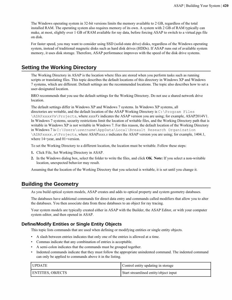
ASAP | Building Your System | 420
The Windows operating system in 32-bit versions limits the memory available to 2 GB, regardless of the totalinstalled RAM. The operating system also requires memory of its own. A system with 2 GB of RAM typically canmake, at most, slightly over 1 GB of RAM available for ray data, before forcing ASAP to switch to a virtual.pgs fileon disk.
For faster speed, you may want to consider using SSD (solid-state drive) disks, regardless of the Windows operatingsystem, instead of traditional magnetic disks such as hard disk drives (HDDs). If ASAP runs out of available systemmemory, it uses disk storage. Therefore, ASAP performance improves with the speed of the disk drive systems.
Setting the Working DirectoryThe Working Directory in ASAP is the location where files are stored when you perform tasks such as runningscripts or translating files. This topic describes the default locations of this directory in Windows XP and Windows7 systems, which are different. Default settings are the recommended locations. The topic also describes how to set auser-designated location.
BRO recommends that you use the default settings for the Working Directory. Do not use a shared network drivelocation.
The default settings differ in Windows XP and Windows 7 systems. In Windows XP systems, alldirectories are writable, and the default location of the ASAP Working Directory is C:\Program Files\ASAPxxxxVx\Projects, where xxxxVx indicates the ASAP version you are using; for example, ASAP2014V1.In Windows 7 systems, security restrictions limit the location of writable files, and the Working Directory path that iswritable in Windows XP is not writable in Windows 7. For this reason, the default location of the Working Directoryin Windows 7 is C:\Users\username\AppData\Local\Breault Research Organization\ASAPxxxx.x\Projects, where ASAPxxxx.x indicates the ASAP version you are using; for example, 1404.1,where 14=year, and 01=version.
To set the Working Directory to a different location, the location must be writable. Follow these steps:
1. Click File, Set Working Directory in ASAP.2. In the Windows dialog box, select the folder to write the files, and click OK. Note: If you select a non-writable
location, unexpected behavior may result.
Assuming that the location of the Working Directory that you selected is writable, it is set until you change it.
Building the GeometryAs you build optical system models, ASAP creates and adds to optical property and system geometry databases.
The databases have additional commands for direct data entry and commands called modifiers that allow you to alterthe databases. You then associate data from these databases to an object for ray tracing.
Your system models are typically created either in ASAP with the Builder, the ASAP Editor, or with your computersystem editor, and then opened in ASAP.
Define/Modify Entities or Single Entity ObjectsThis topic lists commands that are used when defining or modifying entities or single entity objects.
• A slash between entries indicates that only one of the entries is allowed at a time.• Commas indicate that any combination of entries is acceptable.• A semi-colon indicates that the commands must be grouped together.• Indented commands indicate that they must follow the appropriate unindented command. The indented command
can only be applied to commands above it in the listing.
UPDATE Control entity updating in storage
ENTITIES, OBJECTS Start streamlined entity/object input
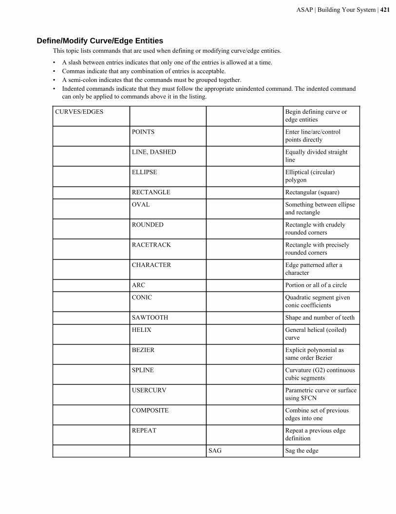
ASAP | Building Your System | 421
Define/Modify Curve/Edge EntitiesThis topic lists commands that are used when defining or modifying curve/edge entities.
• A slash between entries indicates that only one of the entries is allowed at a time.• Commas indicate that any combination of entries is acceptable.• A semi-colon indicates that the commands must be grouped together.• Indented commands indicate that they must follow the appropriate unindented command. The indented command
can only be applied to commands above it in the listing.
CURVES/EDGES Begin defining curve oredge entities
POINTS Enter line/arc/controlpoints directly
LINE, DASHED Equally divided straightline
ELLIPSE Elliptical (circular)polygon
RECTANGLE Rectangular (square)
OVAL Something between ellipseand rectangle
ROUNDED Rectangle with crudelyrounded corners
RACETRACK Rectangle with preciselyrounded corners
CHARACTER Edge patterned after acharacter
ARC Portion or all of a circle
CONIC Quadratic segment givenconic coefficients
SAWTOOTH Shape and number of teeth
HELIX General helical (coiled)curve
BEZIER Explicit polynomial assame order Bezier
SPLINE Curvature (G2) continuouscubic segments
USERCURV Parametric curve or surfaceusing $FCN
COMPOSITE Combine set of previousedges into one
REPEAT Repeat a previous edgedefinition
SAG Sag the edge
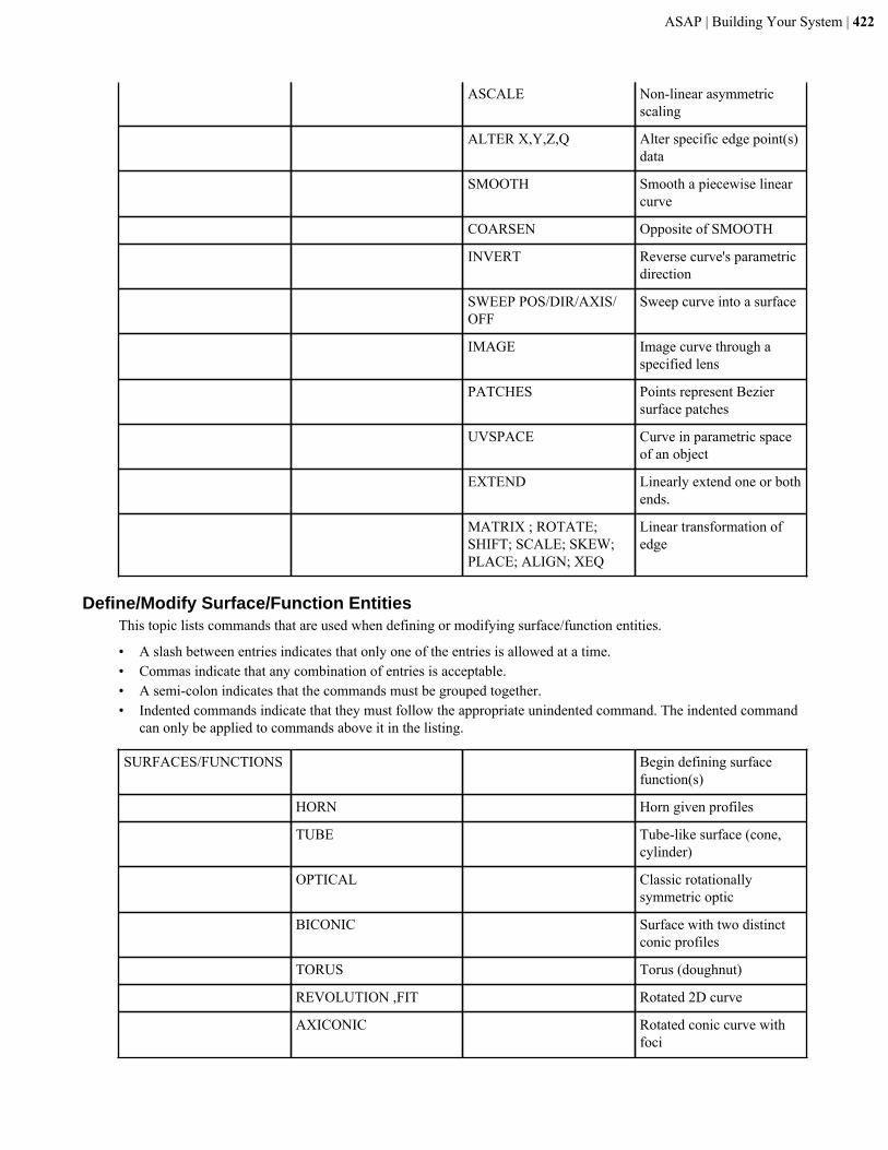
ASAP | Building Your System | 422
ASCALE Non-linear asymmetricscaling
ALTER X,Y,Z,Q Alter specific edge point(s)data
SMOOTH Smooth a piecewise linearcurve
COARSEN Opposite of SMOOTH
INVERT Reverse curve's parametricdirection
SWEEP POS/DIR/AXIS/OFF
Sweep curve into a surface
IMAGE Image curve through aspecified lens
PATCHES Points represent Beziersurface patches
UVSPACE Curve in parametric spaceof an object
EXTEND Linearly extend one or bothends.
MATRIX ; ROTATE;SHIFT; SCALE; SKEW;PLACE; ALIGN; XEQ
Linear transformation ofedge
Define/Modify Surface/Function EntitiesThis topic lists commands that are used when defining or modifying surface/function entities.
• A slash between entries indicates that only one of the entries is allowed at a time.• Commas indicate that any combination of entries is acceptable.• A semi-colon indicates that the commands must be grouped together.• Indented commands indicate that they must follow the appropriate unindented command. The indented command
can only be applied to commands above it in the listing.
SURFACES/FUNCTIONS Begin defining surfacefunction(s)
HORN Horn given profiles
TUBE Tube-like surface (cone,cylinder)
OPTICAL Classic rotationallysymmetric optic
BICONIC Surface with two distinctconic profiles
TORUS Torus (doughnut)
REVOLUTION ,FIT Rotated 2D curve
AXICONIC Rotated conic curve withfoci
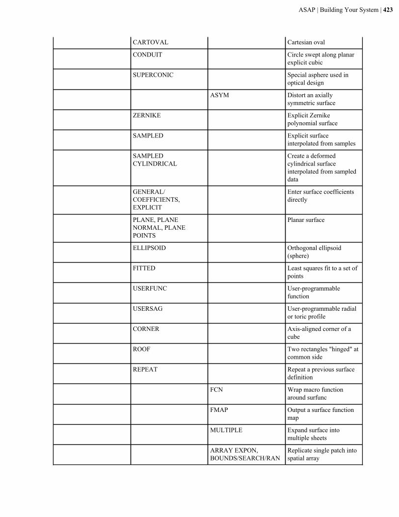
ASAP | Building Your System | 423
CARTOVAL Cartesian oval
CONDUIT Circle swept along planarexplicit cubic
SUPERCONIC Special asphere used inoptical design
ASYM Distort an axiallysymmetric surface
ZERNIKE Explicit Zernikepolynomial surface
SAMPLED Explicit surfaceinterpolated from samples
SAMPLEDCYLINDRICAL
Create a deformedcylindrical surfaceinterpolated from sampleddata
GENERAL/COEFFICIENTS,EXPLICIT
Enter surface coefficientsdirectly
PLANE, PLANENORMAL, PLANEPOINTS
Planar surface
ELLIPSOID Orthogonal ellipsoid(sphere)
FITTED Least squares fit to a set ofpoints
USERFUNC User-programmablefunction
USERSAG User-programmable radialor toric profile
CORNER Axis-aligned corner of acube
ROOF Two rectangles "hinged" atcommon side
REPEAT Repeat a previous surfacedefinition
FCN Wrap macro functionaround surfunc
FMAP Output a surface functionmap
MULTIPLE Expand surface intomultiple sheets
ARRAY EXPON,BOUNDS/SEARCH/RAN
Replicate single patch intospatial array
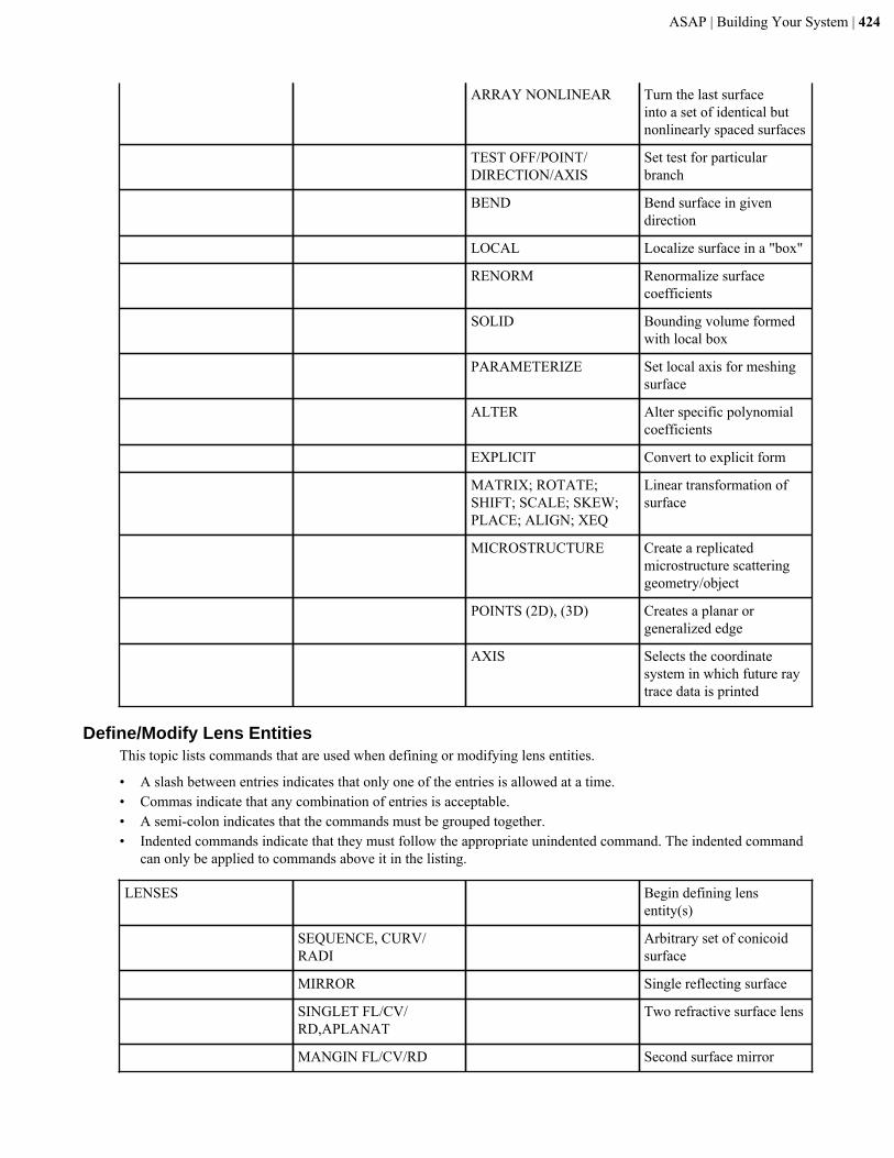
ASAP | Building Your System | 424
ARRAY NONLINEAR Turn the last surfaceinto a set of identical butnonlinearly spaced surfaces
TEST OFF/POINT/DIRECTION/AXIS
Set test for particularbranch
BEND Bend surface in givendirection
LOCAL Localize surface in a "box"
RENORM Renormalize surfacecoefficients
SOLID Bounding volume formedwith local box
PARAMETERIZE Set local axis for meshingsurface
ALTER Alter specific polynomialcoefficients
EXPLICIT Convert to explicit form
MATRIX; ROTATE;SHIFT; SCALE; SKEW;PLACE; ALIGN; XEQ
Linear transformation ofsurface
MICROSTRUCTURE Create a replicatedmicrostructure scatteringgeometry/object
POINTS (2D), (3D) Creates a planar orgeneralized edge
AXIS Selects the coordinatesystem in which future raytrace data is printed
Define/Modify Lens EntitiesThis topic lists commands that are used when defining or modifying lens entities.
• A slash between entries indicates that only one of the entries is allowed at a time.• Commas indicate that any combination of entries is acceptable.• A semi-colon indicates that the commands must be grouped together.• Indented commands indicate that they must follow the appropriate unindented command. The indented command
can only be applied to commands above it in the listing.
LENSES Begin defining lensentity(s)
SEQUENCE, CURV/RADI
Arbitrary set of conicoidsurface
MIRROR Single reflecting surface
SINGLET FL/CV/RD,APLANAT
Two refractive surface lens
MANGIN FL/CV/RD Second surface mirror
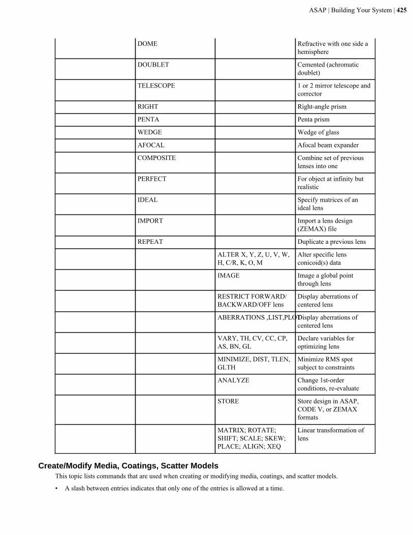
ASAP | Building Your System | 425
DOME Refractive with one side ahemisphere
DOUBLET Cemented (achromaticdoublet)
TELESCOPE 1 or 2 mirror telescope andcorrector
RIGHT Right-angle prism
PENTA Penta prism
WEDGE Wedge of glass
AFOCAL Afocal beam expander
COMPOSITE Combine set of previouslenses into one
PERFECT For object at infinity butrealistic
IDEAL Specify matrices of anideal lens
IMPORT Import a lens design(ZEMAX) file
REPEAT Duplicate a previous lens
ALTER X, Y, Z, U, V, W,H, C/R, K, O, M
Alter specific lensconicoid(s) data
IMAGE Image a global pointthrough lens
RESTRICT FORWARD/BACKWARD/OFF lens
Display aberrations ofcentered lens
ABERRATIONS ,LIST,PLOTDisplay aberrations ofcentered lens
VARY, TH, CV, CC, CP,AS, BN, GL
Declare variables foroptimizing lens
MINIMIZE, DIST, TLEN,GLTH
Minimize RMS spotsubject to constraints
ANALYZE Change 1st-orderconditions, re-evaluate
STORE Store design in ASAP,CODE V, or ZEMAXformats
MATRIX; ROTATE;SHIFT; SCALE; SKEW;PLACE; ALIGN; XEQ
Linear transformation oflens
Create/Modify Media, Coatings, Scatter ModelsThis topic lists commands that are used when creating or modifying media, coatings, and scatter models.
• A slash between entries indicates that only one of the entries is allowed at a time.
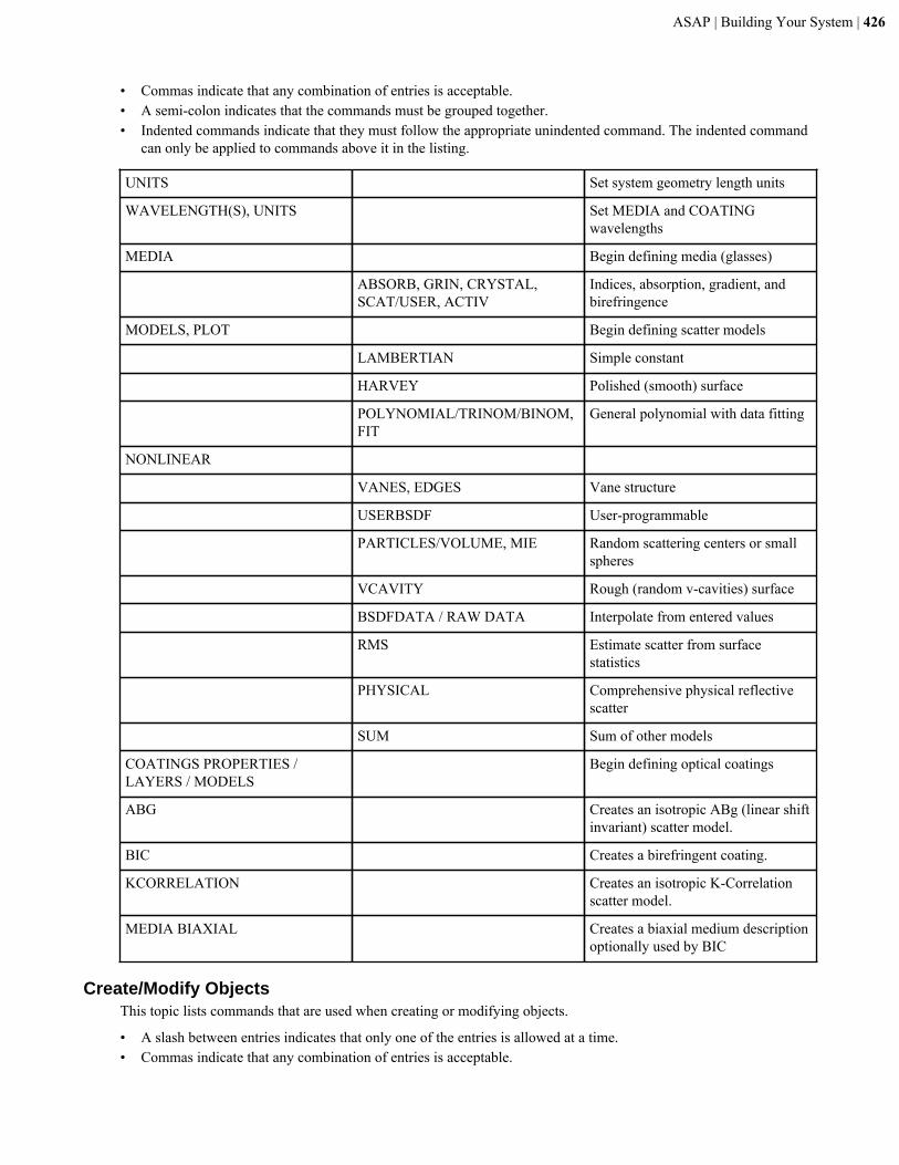
ASAP | Building Your System | 426
• Commas indicate that any combination of entries is acceptable.• A semi-colon indicates that the commands must be grouped together.• Indented commands indicate that they must follow the appropriate unindented command. The indented command
can only be applied to commands above it in the listing.
UNITS Set system geometry length units
WAVELENGTH(S), UNITS Set MEDIA and COATINGwavelengths
MEDIA Begin defining media (glasses)
ABSORB, GRIN, CRYSTAL,SCAT/USER, ACTIV
Indices, absorption, gradient, andbirefringence
MODELS, PLOT Begin defining scatter models
LAMBERTIAN Simple constant
HARVEY Polished (smooth) surface
POLYNOMIAL/TRINOM/BINOM,FIT
General polynomial with data fitting
NONLINEAR
VANES, EDGES Vane structure
USERBSDF User-programmable
PARTICLES/VOLUME, MIE Random scattering centers or smallspheres
VCAVITY Rough (random v-cavities) surface
BSDFDATA / RAW DATA Interpolate from entered values
RMS Estimate scatter from surfacestatistics
PHYSICAL Comprehensive physical reflectivescatter
SUM Sum of other models
COATINGS PROPERTIES /LAYERS / MODELS
Begin defining optical coatings
ABG Creates an isotropic ABg (linear shiftinvariant) scatter model.
BIC Creates a birefringent coating.
KCORRELATION Creates an isotropic K-Correlationscatter model.
MEDIA BIAXIAL Creates a biaxial medium descriptionoptionally used by BIC
Create/Modify ObjectsThis topic lists commands that are used when creating or modifying objects.
• A slash between entries indicates that only one of the entries is allowed at a time.• Commas indicate that any combination of entries is acceptable.
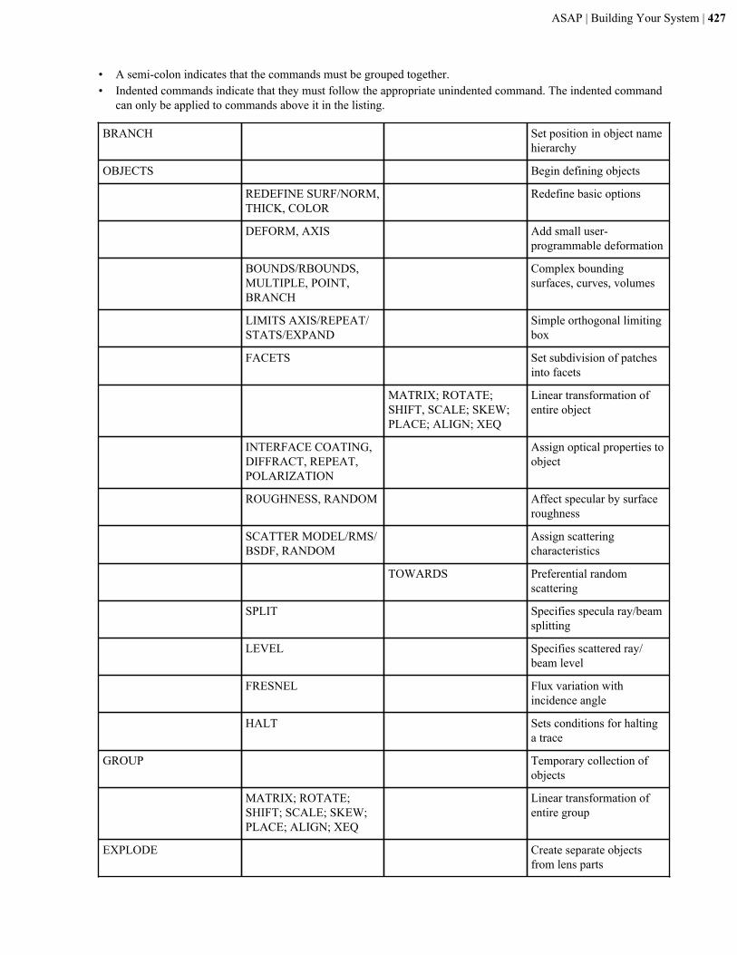
ASAP | Building Your System | 427
• A semi-colon indicates that the commands must be grouped together.• Indented commands indicate that they must follow the appropriate unindented command. The indented command
can only be applied to commands above it in the listing.
BRANCH Set position in object namehierarchy
OBJECTS Begin defining objects
REDEFINE SURF/NORM,THICK, COLOR
Redefine basic options
DEFORM, AXIS Add small user-programmable deformation
BOUNDS/RBOUNDS,MULTIPLE, POINT,BRANCH
Complex boundingsurfaces, curves, volumes
LIMITS AXIS/REPEAT/STATS/EXPAND
Simple orthogonal limitingbox
FACETS Set subdivision of patchesinto facets
MATRIX; ROTATE;SHIFT, SCALE; SKEW;PLACE; ALIGN; XEQ
Linear transformation ofentire object
INTERFACE COATING,DIFFRACT, REPEAT,POLARIZATION
Assign optical properties toobject
ROUGHNESS, RANDOM Affect specular by surfaceroughness
SCATTER MODEL/RMS/BSDF, RANDOM
Assign scatteringcharacteristics
TOWARDS Preferential randomscattering
SPLIT Specifies specula ray/beamsplitting
LEVEL Specifies scattered ray/beam level
FRESNEL Flux variation withincidence angle
HALT Sets conditions for haltinga trace
GROUP Temporary collection ofobjects
MATRIX; ROTATE;SHIFT; SCALE; SKEW;PLACE; ALIGN; XEQ
Linear transformation ofentire group
EXPLODE Create separate objectsfrom lens parts
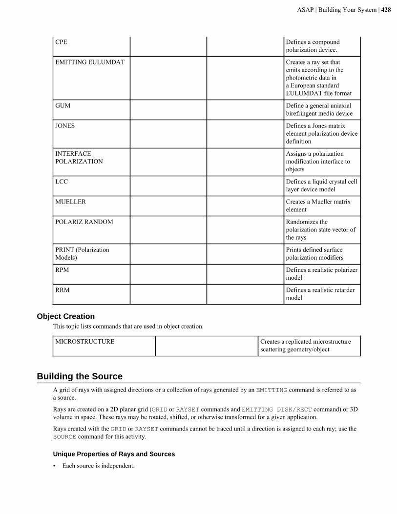
ASAP | Building Your System | 428
CPE Defines a compoundpolarization device.
EMITTING EULUMDAT Creates a ray set thatemits according to thephotometric data ina European standardEULUMDAT file format
GUM Define a general uniaxialbirefringent media device
JONES Defines a Jones matrixelement polarization devicedefinition
INTERFACEPOLARIZATION
Assigns a polarizationmodification interface toobjects
LCC Defines a liquid crystal celllayer device model
MUELLER Creates a Mueller matrixelement
POLARIZ RANDOM Randomizes thepolarization state vector ofthe rays
PRINT (PolarizationModels)
Prints defined surfacepolarization modifiers
RPM Defines a realistic polarizermodel
RRM Defines a realistic retardermodel
Object CreationThis topic lists commands that are used in object creation.
MICROSTRUCTURE Creates a replicated microstructurescattering geometry/object
Building the SourceA grid of rays with assigned directions or a collection of rays generated by an EMITTING command is referred to asa source.
Rays are created on a 2D planar grid (GRID or RAYSET commands and EMITTING DISK/RECT command) or 3Dvolume in space. These rays may be rotated, shifted, or otherwise transformed for a given application.
Rays created with the GRID or RAYSET commands cannot be traced until a direction is assigned to each ray; use theSOURCE command for this activity.
Unique Properties of Rays and Sources
• Each source is independent.
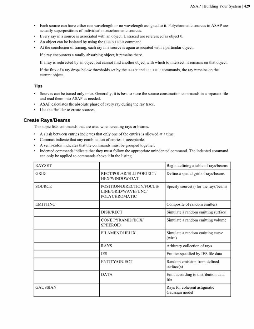
ASAP | Building Your System | 429
• Each source can have either one wavelength or no wavelength assigned to it. Polychromatic sources in ASAP areactually superpositions of individual monochromatic sources.
• Every ray in a source is associated with an object. Untraced are referenced as object 0.• An object can be isolated by using the CONSIDER command.• At the conclusion of tracing, each ray in a source is again associated with a particular object.
If a ray encounters a totally absorbing object, it remains there.
If a ray is redirected by an object but cannot find another object with which to intersect, it remains on that object.
If the flux of a ray drops below thresholds set by the HALT and CUTOFF commands, the ray remains on thecurrent object.
Tips
• Sources can be traced only once. Generally, it is best to store the source construction commands in a separate fileand read them into ASAP as needed.
• ASAP calculates the absolute phase of every ray during the ray trace.• Use the Builder to create sources.
Create Rays/BeamsThis topic lists commands that are used when creating rays or beams.
• A slash between entries indicates that only one of the entries is allowed at a time.• Commas indicate that any combination of entries is acceptable.• A semi-colon indicates that the commands must be grouped together.• Indented commands indicate that they must follow the appropriate unindented command. The indented command
can only be applied to commands above it in the listing.
RAYSET Begin defining a table of rays/beams
GRID RECT/POLAR/ELLIP/OBJECT/HEX/WINDOW/DAT
Define a spatial grid of rays/beams
SOURCE POSITION/DIRECTION/FOCUS/LINE/GRID/WAVEFUNC/POLYCHROMATIC
Specify source(s) for the rays/beams
EMITTING Composite of random emitters
DISK/RECT Simulate a random emitting surface
CONE PYRAMID/BOX/SPHEROID
Simulate a random emitting volume
FILAMENT/HELIX Simulate a random emitting curve(wire)
RAYS Arbitrary collection of rays
IES Emitter specified by IES file data
ENTITY/OBJECT Random emission from definedsurface(s)
DATA Emit according to distribution datafile
GAUSSIAN Rays for coherent astigmaticGaussian model
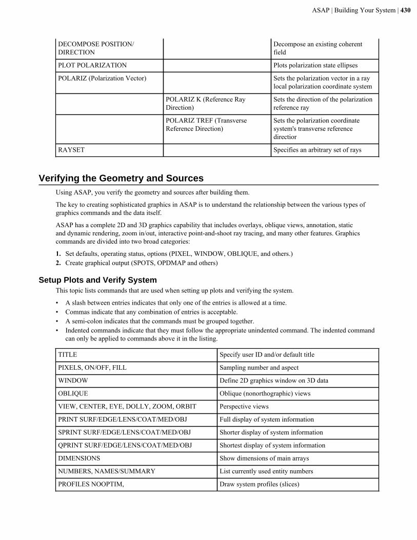
ASAP | Building Your System | 430
DECOMPOSE POSITION/DIRECTION
Decompose an existing coherentfield
PLOT POLARIZATION Plots polarization state ellipses
POLARIZ (Polarization Vector) Sets the polarization vector in a raylocal polarization coordinate system
POLARIZ K (Reference RayDirection)
Sets the direction of the polarizationreference ray
POLARIZ TREF (TransverseReference Direction)
Sets the polarization coordinatesystem's transverse referencedirectior
RAYSET Specifies an arbitrary set of rays
Verifying the Geometry and SourcesUsing ASAP, you verify the geometry and sources after building them.
The key to creating sophisticated graphics in ASAP is to understand the relationship between the various types ofgraphics commands and the data itself.
ASAP has a complete 2D and 3D graphics capability that includes overlays, oblique views, annotation, staticand dynamic rendering, zoom in/out, interactive point-and-shoot ray tracing, and many other features. Graphicscommands are divided into two broad categories:
1. Set defaults, operating status, options (PIXEL, WINDOW, OBLIQUE, and others.)2. Create graphical output (SPOTS, OPDMAP and others)
Setup Plots and Verify SystemThis topic lists commands that are used when setting up plots and verifying the system.
• A slash between entries indicates that only one of the entries is allowed at a time.• Commas indicate that any combination of entries is acceptable.• A semi-colon indicates that the commands must be grouped together.• Indented commands indicate that they must follow the appropriate unindented command. The indented command
can only be applied to commands above it in the listing.
TITLE Specify user ID and/or default title
PIXELS, ON/OFF, FILL Sampling number and aspect
WINDOW Define 2D graphics window on 3D data
OBLIQUE Oblique (nonorthographic) views
VIEW, CENTER, EYE, DOLLY, ZOOM, ORBIT Perspective views
PRINT SURF/EDGE/LENS/COAT/MED/OBJ Full display of system information
SPRINT SURF/EDGE/LENS/COAT/MED/OBJ Shorter display of system information
QPRINT SURF/EDGE/LENS/COAT/MED/OBJ Shortest display of system information
DIMENSIONS Show dimensions of main arrays
NUMBERS, NAMES/SUMMARY List currently used entity numbers
PROFILES NOOPTIM, Draw system profiles (slices)
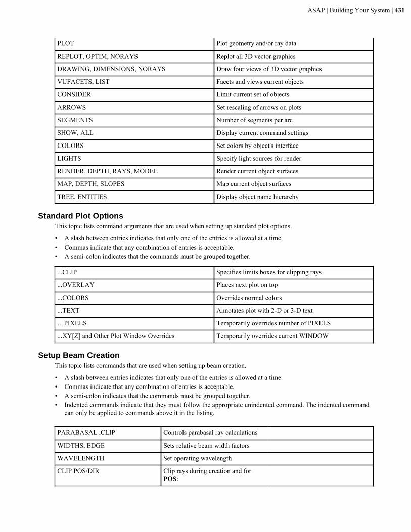
ASAP | Building Your System | 431
PLOT Plot geometry and/or ray data
REPLOT, OPTIM, NORAYS Replot all 3D vector graphics
DRAWING, DIMENSIONS, NORAYS Draw four views of 3D vector graphics
VUFACETS, LIST Facets and views current objects
CONSIDER Limit current set of objects
ARROWS Set rescaling of arrows on plots
SEGMENTS Number of segments per arc
SHOW, ALL Display current command settings
COLORS Set colors by object's interface
LIGHTS Specify light sources for render
RENDER, DEPTH, RAYS, MODEL Render current object surfaces
MAP, DEPTH, SLOPES Map current object surfaces
TREE, ENTITIES Display object name hierarchy
Standard Plot OptionsThis topic lists command arguments that are used when setting up standard plot options.
• A slash between entries indicates that only one of the entries is allowed at a time.• Commas indicate that any combination of entries is acceptable.• A semi-colon indicates that the commands must be grouped together.
...CLIP Specifies limits boxes for clipping rays
...OVERLAY Places next plot on top
...COLORS Overrides normal colors
...TEXT Annotates plot with 2-D or 3-D text
…PIXELS Temporarily overrides number of PIXELS
...XY[Z] and Other Plot Window Overrides Temporarily overrides current WINDOW
Setup Beam CreationThis topic lists commands that are used when setting up beam creation.
• A slash between entries indicates that only one of the entries is allowed at a time.• Commas indicate that any combination of entries is acceptable.• A semi-colon indicates that the commands must be grouped together.• Indented commands indicate that they must follow the appropriate unindented command. The indented command
can only be applied to commands above it in the listing.
PARABASAL ,CLIP Controls parabasal ray calculations
WIDTHS, EDGE Sets relative beam width factors
WAVELENGTH Set operating wavelength
CLIP POS/DIR Clip rays during creation and forPOS:
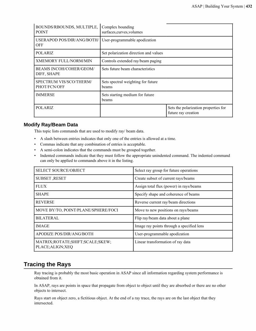
ASAP | Building Your System | 432
BOUNDS/RBOUNDS, MULTIPLE,POINT
Complex boundingsurfaces,curves,volumes
USERAPOD POS/DIR/ANG/BOTH/OFF
User-programmable apodization
POLARIZ Set polarization direction and values
XMEMORY FULL/NORM/MIN Controls extended ray/beam paging
BEAMS INCOH/COHER/GEOM/DIFF, SHAPE
Sets future beam characteristics
SPECTRUM VIS/SCO/THERM/PHOT/FCN/OFF
Sets spectral weighting for futurebeams
IMMERSE Sets starting medium for futurebeams
POLARIZ Sets the polarization properties forfuture ray creation
Modify Ray/Beam DataThis topic lists commands that are used to modify ray/ beam data.
• A slash between entries indicates that only one of the entries is allowed at a time.• Commas indicate that any combination of entries is acceptable.• A semi-colon indicates that the commands must be grouped together.• Indented commands indicate that they must follow the appropriate unindented command. The indented command
can only be applied to commands above it in the listing.
SELECT SOURCE/OBJECT Select ray group for future operations
SUBSET ,RESET Create subset of current rays/beams
FLUX Assign total flux (power) in rays/beams
SHAPE Specify shape and coherence of beams
REVERSE Reverse current ray/beam directions
MOVE BY/TO, POINT/PLANE/SPHERE/FOCI Move to new positions on rays/beams
BILATERAL Flip ray/beam data about a plane
IMAGE Image ray points through a specified lens
APODIZE POS/DIR/ANG/BOTH User-programmable apodization
MATRIX;ROTATE;SHIFT;SCALE;SKEW;PLACE;ALIGN;XEQ
Linear transformation of ray data
Tracing the RaysRay tracing is probably the most basic operation in ASAP since all information regarding system performance isobtained from it.
In ASAP, rays are points in space that propagate from object to object until they are absorbed or there are no otherobjects to intersect.
Rays start on object zero, a fictitious object. At the end of a ray trace, the rays are on the last object that theyintersected.
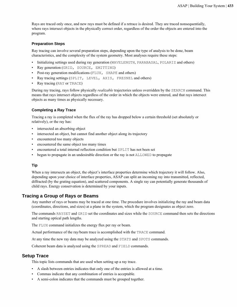
ASAP | Building Your System | 433
Rays are traced only once, and new rays must be defined if a retrace is desired. They are traced nonsequentially,where rays intersect objects in the physically correct order, regardless of the order the objects are entered into theprogram.
Preparation Steps
Ray tracing can involve several preparation steps, depending upon the type of analysis to be done, beamcharacteristics, and the complexity of the system geometry. Most analyses require these steps:
• Initializing settings used during ray generation (WAVELENGTH, PARABASAL, POLARIZ and others)• Ray generation (GRID, SOURCE, EMITTING)• Post-ray generation modifications (FLUX, SHAPE and others)• Ray tracing settings (SPLIT, LEVEL, AXIS, FRESNEL and others)• Ray tracing (RAY or TRACE)
During ray tracing, rays follow physically realizable trajectories unless overridden by the SEARCH command. Thismeans that rays intersect objects regardless of the order in which the objects were entered, and that rays intersectobjects as many times as physically necessary.
Completing a Ray Trace
Tracing a ray is completed when the flux of the ray has dropped below a certain threshold (set absolutely orrelatively), or the ray has:
• intersected an absorbing object• intersected an object, but cannot find another object along its trajectory• encountered too many objects• encountered the same object too many times• encountered a total internal reflection condition but SPLIT has not been set• begun to propagate in an undesirable direction or the ray is not ALLOWED to propagate
Tip
When a ray intersects an object, the object’s interface properties determine which trajectory it will follow. Also,depending upon your choice of interface properties, ASAP can split an incoming ray into transmitted, reflected,diffracted (by the grating equation), and scattered components. A single ray can potentially generate thousands ofchild rays. Energy conservation is determined by your inputs.
Tracing a Group of Rays or BeamsAny number of rays or beams may be traced at one time. The procedure involves initializing the ray and beam data(coordinates, directions, and sizes) at a plane in the system, which the program designates as object zero.
The commands RAYSET and GRID set the coordinates and sizes while the SOURCE command then sets the directionsand starting optical path lengths.
The FLUX command initializes the energy flux per ray or beam.
Actual performance of the ray/beam trace is accomplished with the TRACE command.
At any time the new ray data may be analyzed using the STATS and SPOTS commands.
Coherent beam data is analyzed using the SPREAD and FIELD commands.
Setup TraceThis topic lists commands that are used when setting up a ray trace.
• A slash between entries indicates that only one of the entries is allowed at a time.• Commas indicate that any combination of entries is acceptable.• A semi-colon indicates that the commands must be grouped together.
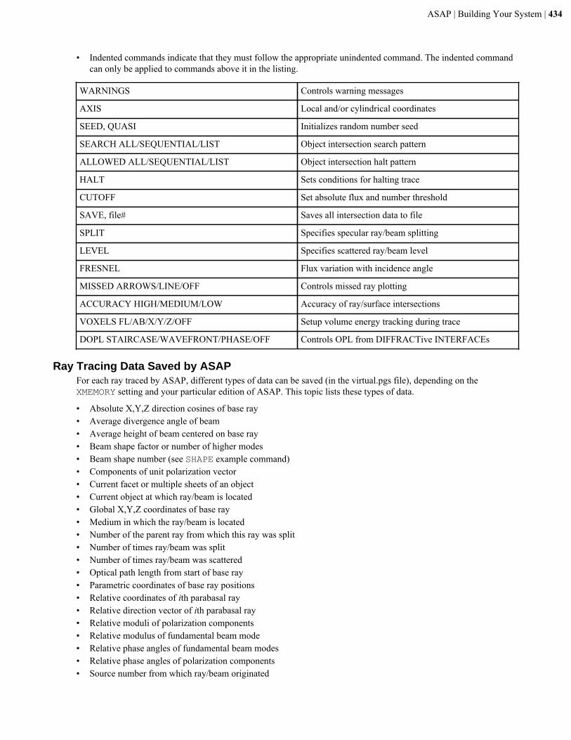
ASAP | Building Your System | 434
• Indented commands indicate that they must follow the appropriate unindented command. The indented commandcan only be applied to commands above it in the listing.
WARNINGS Controls warning messages
AXIS Local and/or cylindrical coordinates
SEED, QUASI Initializes random number seed
SEARCH ALL/SEQUENTIAL/LIST Object intersection search pattern
ALLOWED ALL/SEQUENTIAL/LIST Object intersection halt pattern
HALT Sets conditions for halting trace
CUTOFF Set absolute flux and number threshold
SAVE, file# Saves all intersection data to file
SPLIT Specifies specular ray/beam splitting
LEVEL Specifies scattered ray/beam level
FRESNEL Flux variation with incidence angle
MISSED ARROWS/LINE/OFF Controls missed ray plotting
ACCURACY HIGH/MEDIUM/LOW Accuracy of ray/surface intersections
VOXELS FL/AB/X/Y/Z/OFF Setup volume energy tracking during trace
DOPL STAIRCASE/WAVEFRONT/PHASE/OFF Controls OPL from DIFFRACTive INTERFACEs
Ray Tracing Data Saved by ASAPFor each ray traced by ASAP, different types of data can be saved (in the virtual.pgs file), depending on theXMEMORY setting and your particular edition of ASAP. This topic lists these types of data.
• Absolute X,Y,Z direction cosines of base ray• Average divergence angle of beam• Average height of beam centered on base ray• Beam shape factor or number of higher modes• Beam shape number (see SHAPE example command)• Components of unit polarization vector• Current facet or multiple sheets of an object• Current object at which ray/beam is located• Global X,Y,Z coordinates of base ray• Medium in which the ray/beam is located• Number of the parent ray from which this ray was split• Number of times ray/beam was split• Number of times ray/beam was scattered• Optical path length from start of base ray• Parametric coordinates of base ray positions• Relative coordinates of ith parabasal ray• Relative direction vector of ith parabasal ray• Relative moduli of polarization components• Relative modulus of fundamental beam mode• Relative phase angles of fundamental beam modes• Relative phase angles of polarization components• Source number from which ray/beam originated

ASAP | Building Your System | 435
• The ith previous split object for ray/beam• Total flux in ray/beam• Total number of objects ray has intersected• Total number of original sources• Total number of rays/beams• Wavelength of ith source• Wavelength of ray/beam
Trace Ray and BeamsThis topic lists commands that are used when performing a ray/beam trace.
• A slash between entries indicates that only one of the entries is allowed at a time.• Commas indicate that any combination of entries is acceptable.• A semi-colon indicates that the commands must be grouped together.• Indented commands indicate that they must follow the appropriate unindented command. The indented command
can only be applied to commands above it in the listing.
RAY, PLOT, DIR, SEARCH, GALOP, LENS Trace a single ray
TRACE, PLOT/GRA, LIST/DIR, STATS, STEP Trace current set of rays/beams
Analyzing the DataAt the conclusion of ray tracing, the rays are ready for the next operation, which is usually an analysis function.
Unlike most optical design programs that produce ray-tracing output, ASAP treats ray tracing as simply an operationon the ray data.
The analysis commands in ASAP access the ray data stored in the file, VIRTUAL.PGS and operate on the ray dataaccordingly. In some cases, the action of the analysis command changes the ray data; for example, a MOVE commanddetermines the position of best focus in three dimensions and translates the ray data along their trajectories to thiscoordinate.
Alternatively, the command produces a plot of the ray coordinates within the currently defined window, and doesnot modify the ray data in any way. The action depends upon the specific command or the specific option within thecommand.
Analyze Ray/Beam DataThis topic lists commands that are used when analyzing ray/beam data.
• A slash between entries indicates that only one of the entries is allowed at a time.• Commas indicate that any combination of entries is acceptable.• A semi-colon indicates that the commands must be grouped together.• Indented commands indicate that they must follow the appropriate unindented command. The indented command
can only be applied to commands above it in the listing.
LIST POS/DIR/RAY/SOU/INT/ELL List specific data for all or some rays
EXTREMES POS/DIR/FLUX/LEN List data on extreme rays
STATS POSITION/DIRECTION Statistics of ray/beam data by object
PATHS AVE/PEAK/TOT/OBJ Grouping and listing of ray path
HISTORY, PLOT Display histories of rays in SAVE file
SPOTS POSITION/DIRECTION Distribution of current ray data
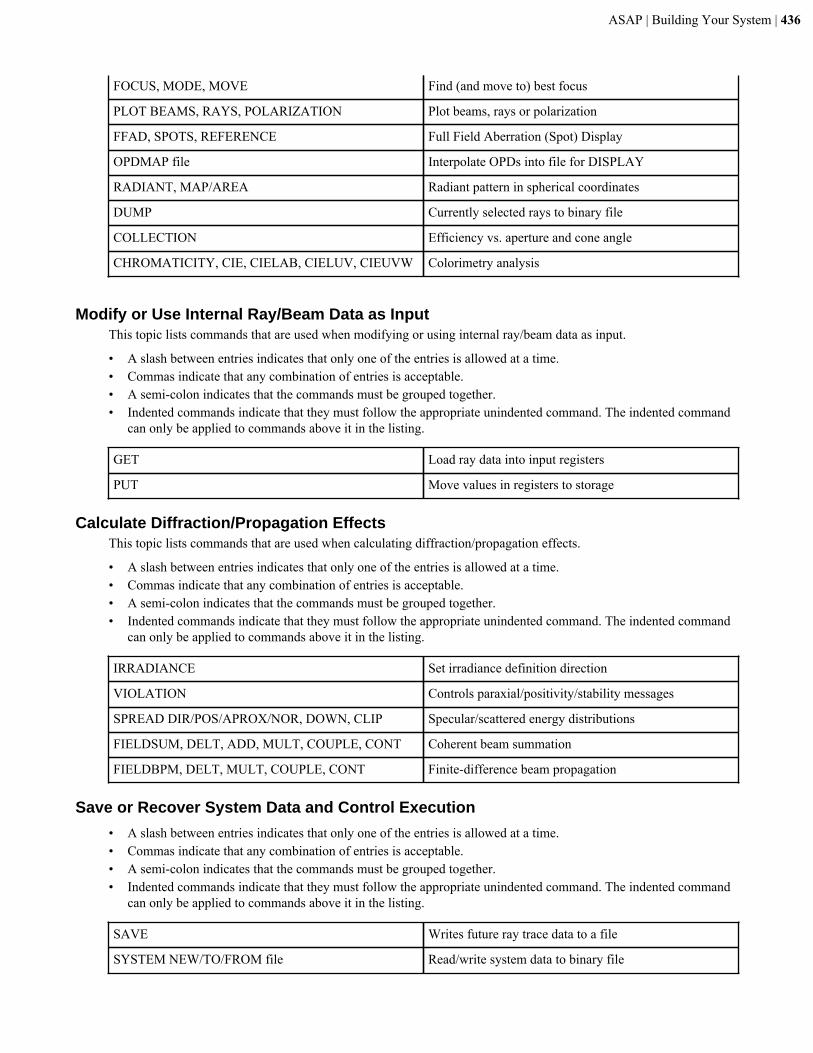
ASAP | Building Your System | 436
FOCUS, MODE, MOVE Find (and move to) best focus
PLOT BEAMS, RAYS, POLARIZATION Plot beams, rays or polarization
FFAD, SPOTS, REFERENCE Full Field Aberration (Spot) Display
OPDMAP file Interpolate OPDs into file for DISPLAY
RADIANT, MAP/AREA Radiant pattern in spherical coordinates
DUMP Currently selected rays to binary file
COLLECTION Efficiency vs. aperture and cone angle
CHROMATICITY, CIE, CIELAB, CIELUV, CIEUVW Colorimetry analysis
Modify or Use Internal Ray/Beam Data as InputThis topic lists commands that are used when modifying or using internal ray/beam data as input.
• A slash between entries indicates that only one of the entries is allowed at a time.• Commas indicate that any combination of entries is acceptable.• A semi-colon indicates that the commands must be grouped together.• Indented commands indicate that they must follow the appropriate unindented command. The indented command
can only be applied to commands above it in the listing.
GET Load ray data into input registers
PUT Move values in registers to storage
Calculate Diffraction/Propagation EffectsThis topic lists commands that are used when calculating diffraction/propagation effects.
• A slash between entries indicates that only one of the entries is allowed at a time.• Commas indicate that any combination of entries is acceptable.• A semi-colon indicates that the commands must be grouped together.• Indented commands indicate that they must follow the appropriate unindented command. The indented command
can only be applied to commands above it in the listing.
IRRADIANCE Set irradiance definition direction
VIOLATION Controls paraxial/positivity/stability messages
SPREAD DIR/POS/APROX/NOR, DOWN, CLIP Specular/scattered energy distributions
FIELDSUM, DELT, ADD, MULT, COUPLE, CONT Coherent beam summation
FIELDBPM, DELT, MULT, COUPLE, CONT Finite-difference beam propagation
Save or Recover System Data and Control Execution
• A slash between entries indicates that only one of the entries is allowed at a time.• Commas indicate that any combination of entries is acceptable.• A semi-colon indicates that the commands must be grouped together.• Indented commands indicate that they must follow the appropriate unindented command. The indented command
can only be applied to commands above it in the listing.
SAVE Writes future ray trace data to a file
SYSTEM NEW/TO/FROM file Read/write system data to binary file
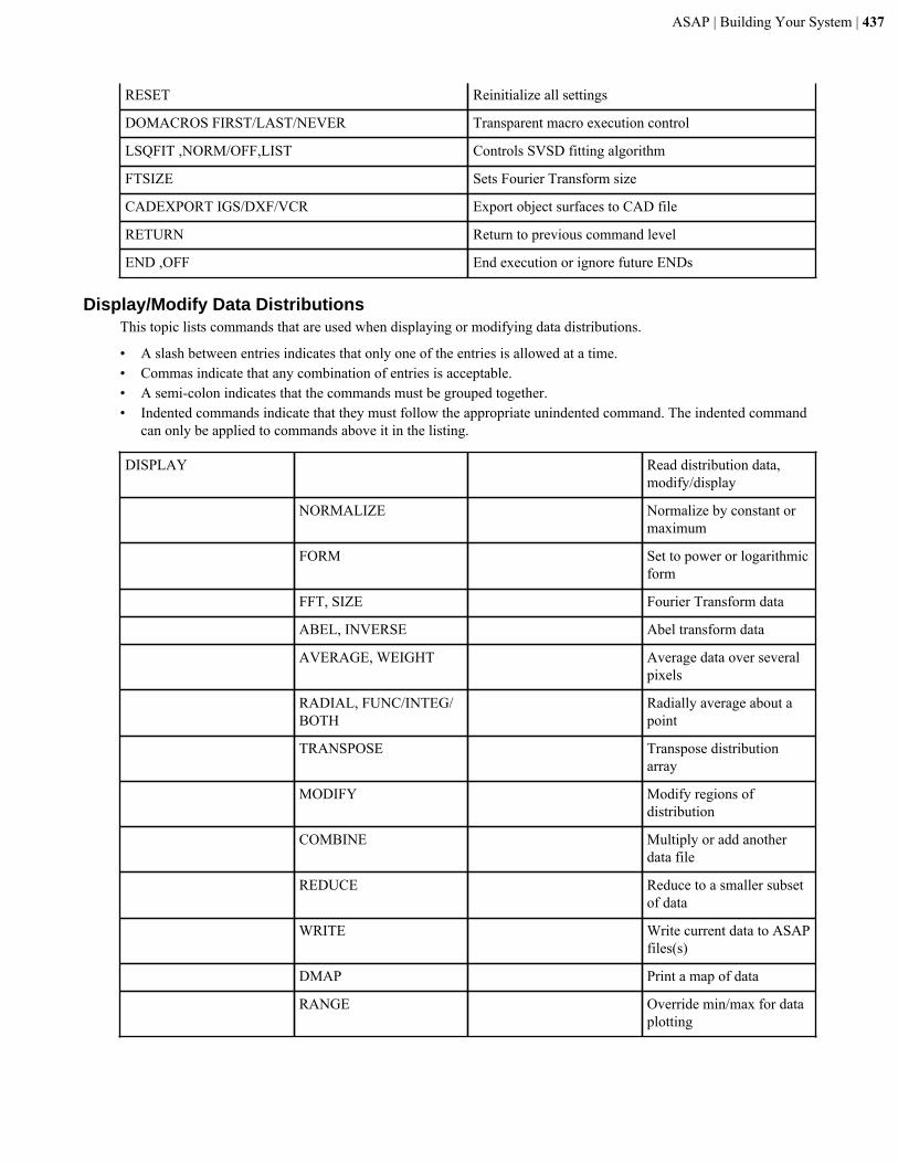
ASAP | Building Your System | 437
RESET Reinitialize all settings
DOMACROS FIRST/LAST/NEVER Transparent macro execution control
LSQFIT ,NORM/OFF,LIST Controls SVSD fitting algorithm
FTSIZE Sets Fourier Transform size
CADEXPORT IGS/DXF/VCR Export object surfaces to CAD file
RETURN Return to previous command level
END ,OFF End execution or ignore future ENDs
Display/Modify Data DistributionsThis topic lists commands that are used when displaying or modifying data distributions.
• A slash between entries indicates that only one of the entries is allowed at a time.• Commas indicate that any combination of entries is acceptable.• A semi-colon indicates that the commands must be grouped together.• Indented commands indicate that they must follow the appropriate unindented command. The indented command
can only be applied to commands above it in the listing.
DISPLAY Read distribution data,modify/display
NORMALIZE Normalize by constant ormaximum
FORM Set to power or logarithmicform
FFT, SIZE Fourier Transform data
ABEL, INVERSE Abel transform data
AVERAGE, WEIGHT Average data over severalpixels
RADIAL, FUNC/INTEG/BOTH
Radially average about apoint
TRANSPOSE Transpose distributionarray
MODIFY Modify regions ofdistribution
COMBINE Multiply or add anotherdata file
REDUCE Reduce to a smaller subsetof data
WRITE Write current data to ASAPfiles(s)
DMAP Print a map of data
RANGE Override min/max for dataplotting
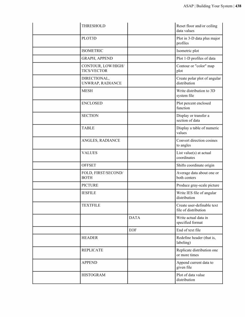
ASAP | Building Your System | 438
THRESHOLD Reset floor and/or ceilingdata values
PLOT3D Plot in 3-D data plus majorprofiles
ISOMETRIC Isometric plot
GRAPH, APPEND Plot 1-D profiles of data
CONTOUR, LOW/HIGH/TICS/VECTOR
Contour or "color" mapplot
DIRECTIONAL,UNWRAP, RADIANCE
Create polar plot of angulardistribution
MESH Write distribution to 3Dsystem file
ENCLOSED Plot percent enclosedfunction
SECTION Display or transfer asection of data
TABLE Display a table of numericvalues
ANGLES, RADIANCE Convert direction cosinesto angles
VALUES List value(s) at actualcoordinates
OFFSET Shifts coordinate origin
FOLD, FIRST/SECOND/BOTH
Average data about one orboth centers
PICTURE Produce gray-scale picture
IESFILE Write IES file of angulardistribution
TEXTFILE Create user-definable textfile of distribution
DATA Write actual data inspecified format
EOF End of text file
HEADER Redefine header (that is,labeling)
REPLICATE Replicate distribution oneor more times
APPEND Append current data togiven file
HISTOGRAM Plot of data valuedistribution

ASAP | Building Your System | 439
TERRAIN Peaks/valleys and FWHMstatistics
REMOVE Subtract best-fitpolynomial
ELUMDATFILE Writes out anEULUMDAT format file
ASAP | Kernel Capabilities Overview | 440
Kernel Capabilities Overview
This topic briefly describes how ASAP models optical/mechanical systems, traces rays through the system, andmodels physical optics.
Modeling Optical-Mechanical Systems
ASAP accurately models virtually any optical-mechanical systems. Similar to 3D solids modeling programs,it utilizes a powerful geometrical approach that permits a nearly limitless variety of systems to be handled in astraightforward manner. As opposed to most other ray tracing algorithms, all surfaces and ray data are referenced bydefault to a single global Cartesian coordinate system. Smooth continuous object surfaces can be represented by asequence of simple conicoids or a general 286-term polynomial (taken to 10th or 20th-order in the three Cartesiancomponents or their squares), and can be bounded by other surfaces of the same general form. Therefore, anythingfrom a simple plane with a polygonal boundary to an arbitrarily oriented elliptical toroid can be modeled precisely.Even more complex parametric mesh surfaces (NURBS) can be defined by connecting two or more arbitrary curves,each formed by a series of lines and/or conic arcs in space.
Tracing Rays through the System
Bundles of rays can be traced through the system so that, after every reflection or refraction, each ray always transfersto the nearest object. Rays are allowed to interact with an object any number of times; that is, multiple bounces.Therefore, the program easily handles the "funneling" effect of non-imaging radiation collectors as well as imagingsystems. Each ray may be assigned an arbitrary total flux that is reduced by volume and surface absorption (orincreased in a gain medium) as the ray propagates through the system. The standard Fresnel equations are used tonot only calculate (as a function of incidence angle and polarization) transmission losses at interfaces between twodielectric media, but also reflection losses at any dielectric/conductor interfaces. The program is also capable ofsplitting any ray into reflected, transmitted, diffractive, near specular, diffuse, and backscatter components.
Modeling of Physical Optics
Each ray may also be treated as a coherent/incoherent scalar/vector beam (normally Gaussian). Groups of these beamscan be combined to simulate the optical or electromagnetic field incident on a system. Each beam and thus the entire"wavefront" is then rigorously propagated. The resulting field may then be calculated and displayed at any locationwithin the system (including on the surfaces of grazing incidence optics) and not just near focus. ASAP not onlyperforms geometrical optics modeling, but also accurate physical optics modeling of any system.
Command ModeThis topic describes scripting functions available only in command mode.
• Scatter and several other commands.• Macros for performing looping, if-statements, source and geometry libraries; and for reducing frequently used
command sequences to a single command.• User-written files that you can extensively comment and easily read.• Variables and mathematical expressions for defining quantities that are frequently changed.
Note: You can use the command mode interactively or in the background in batch mode. Since the outputfiles are fully compatible with the user interface, you can use the user interface to view or manipulategraphics.
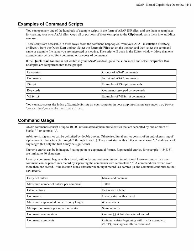
ASAP | Kernel Capabilities Overview | 441
Examples of Command ScriptsYou can open any one of the hundreds of example scripts in the form of ASAP INR files, and use them as templatesfor creating your own ASAP files. Copy all or portions of these examples to the Clipboard, paste them into an Editorwindow.
These scripts are accessible in three ways: from the command help topics, from your ASAP installation directory,or directly from the Quick Start toolbar. Select the Example Files tab on the toolbar, and then select the commandname or example file name you are interested in viewing. The script will open in the Editor window. More than oneexample may be listed for a command or category of commands.
If the Quick Start toolbar is not visible in your ASAP window, go to the View menu and select Properties Bar.Examples are categorized into these groups:
Categories Groups of ASAP commands
Commands Individual ASAP commands
JScript Examples of JScript commands
Keywords Commands grouped by keywords
VBScript Examples of VBScript commands
You can also access the Index of Example Scripts on your computer in your asap installation area under projects\examples\example_scripts.html.
Command UsageASAP commands consist of up to 10,000 unformatted alphanumeric entries that are separated by one or more ofblanks " " or commas ",".
Arbitrary string entries can be delimited by double quotes. Otherwise, literal entries consist of an unbroken string ofalphanumeric characters (A through Z through 9, and _). They must start with a letter or underscore "_" and can be ofany length (but only the first 8 may be significant).
Numeric entries can be in integer, floating point or exponential format. Exponential entries, for example "1.34E-5",are limited to 40 characters.
Usually a command begins with a literal, with only one command in each input record. However, more than onecommand can be placed in a record by separating the commands with semicolons ";". A command can extend overmore than one record. If the last non-blank character in an input record is a comma (,), the command continues to thenext record.
Entry delimiters blanks and commas
Maximum number of entries per command 10000
Literal entries Begin with a letter
Commands Usually start with a literal
Maximum exponential numeric entry length 40 characters
Multiple commands per record separator Semicolon (;)
Command continuation Comma (,) at last character of record
Command arguments Optional entries beginning with …(for example, …CLIP); must appear after a command
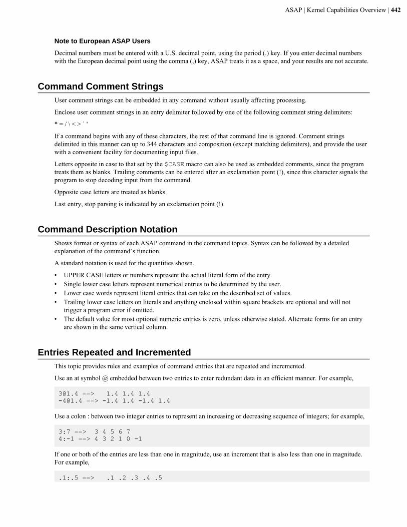
ASAP | Kernel Capabilities Overview | 442
Note to European ASAP Users
Decimal numbers must be entered with a U.S. decimal point, using the period (.) key. If you enter decimal numberswith the European decimal point using the comma (,) key, ASAP treats it as a space, and your results are not accurate.
Command Comment StringsUser comment strings can be embedded in any command without usually affecting processing.
Enclose user comment strings in an entry delimiter followed by one of the following comment string delimiters:
* = / \ < > ` '
If a command begins with any of these characters, the rest of that command line is ignored. Comment stringsdelimited in this manner can up to 344 characters and composition (except matching delimiters), and provide the userwith a convenient facility for documenting input files.
Letters opposite in case to that set by the $CASE macro can also be used as embedded comments, since the programtreats them as blanks. Trailing comments can be entered after an exclamation point (!), since this character signals theprogram to stop decoding input from the command.
Opposite case letters are treated as blanks.
Last entry, stop parsing is indicated by an exclamation point (!).
Command Description NotationShows format or syntax of each ASAP command in the command topics. Syntax can be followed by a detailedexplanation of the command’s function.
A standard notation is used for the quantities shown.
• UPPER CASE letters or numbers represent the actual literal form of the entry.• Single lower case letters represent numerical entries to be determined by the user.• Lower case words represent literal entries that can take on the described set of values.• Trailing lower case letters on literals and anything enclosed within square brackets are optional and will not
trigger a program error if omitted.• The default value for most optional numeric entries is zero, unless otherwise stated. Alternate forms for an entry
are shown in the same vertical column.
Entries Repeated and IncrementedThis topic provides rules and examples of command entries that are repeated and incremented.
Use an at symbol @ embedded between two entries to enter redundant data in an efficient manner. For example,
[email protected] ==> 1.4 1.4 [email protected] ==> -1.4 1.4 -1.4 1.4
Use a colon : between two integer entries to represent an increasing or decreasing sequence of integers; for example,
3:7 ==> 3 4 5 6 74:-1 ==> 4 3 2 1 0 -1
If one or both of the entries are less than one in magnitude, use an increment that is also less than one in magnitude.For example,
.1:.5 ==> .1 .2 .3 .4 .5
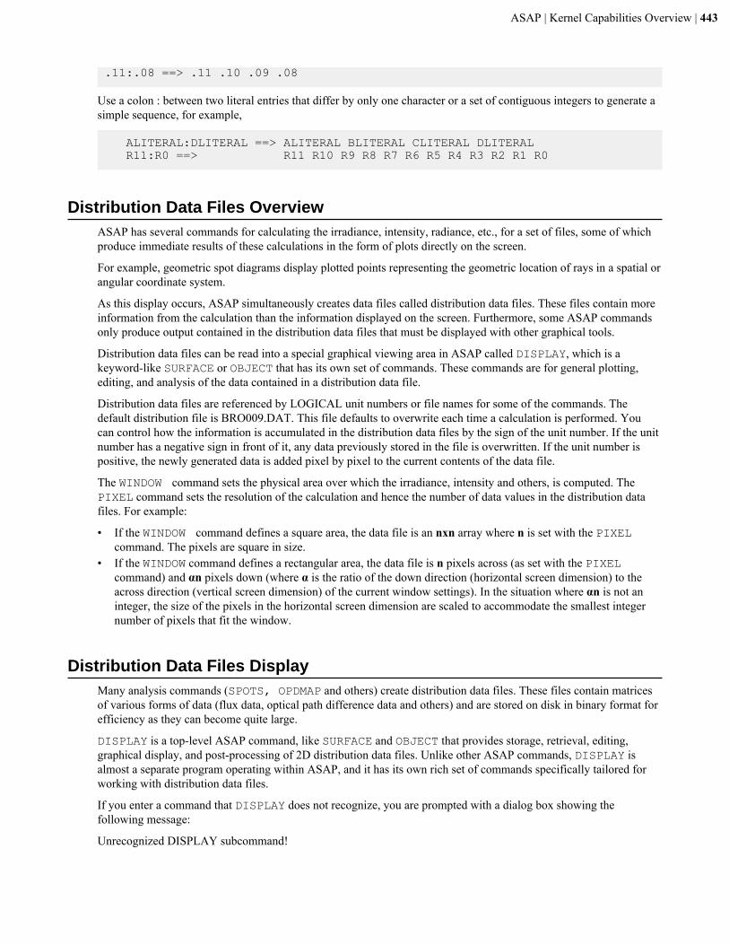
ASAP | Kernel Capabilities Overview | 443
.11:.08 ==> .11 .10 .09 .08
Use a colon : between two literal entries that differ by only one character or a set of contiguous integers to generate asimple sequence, for example,
ALITERAL:DLITERAL ==> ALITERAL BLITERAL CLITERAL DLITERAL R11:R0 ==> R11 R10 R9 R8 R7 R6 R5 R4 R3 R2 R1 R0
Distribution Data Files OverviewASAP has several commands for calculating the irradiance, intensity, radiance, etc., for a set of files, some of whichproduce immediate results of these calculations in the form of plots directly on the screen.
For example, geometric spot diagrams display plotted points representing the geometric location of rays in a spatial orangular coordinate system.
As this display occurs, ASAP simultaneously creates data files called distribution data files. These files contain moreinformation from the calculation than the information displayed on the screen. Furthermore, some ASAP commandsonly produce output contained in the distribution data files that must be displayed with other graphical tools.
Distribution data files can be read into a special graphical viewing area in ASAP called DISPLAY, which is akeyword-like SURFACE or OBJECT that has its own set of commands. These commands are for general plotting,editing, and analysis of the data contained in a distribution data file.
Distribution data files are referenced by LOGICAL unit numbers or file names for some of the commands. Thedefault distribution file is BRO009.DAT. This file defaults to overwrite each time a calculation is performed. Youcan control how the information is accumulated in the distribution data files by the sign of the unit number. If the unitnumber has a negative sign in front of it, any data previously stored in the file is overwritten. If the unit number ispositive, the newly generated data is added pixel by pixel to the current contents of the data file.
The WINDOW command sets the physical area over which the irradiance, intensity and others, is computed. ThePIXEL command sets the resolution of the calculation and hence the number of data values in the distribution datafiles. For example:
• If the WINDOW command defines a square area, the data file is an nxn array where n is set with the PIXEL command. The pixels are square in size.
• If the WINDOW command defines a rectangular area, the data file is n pixels across (as set with the PIXEL command) and αn pixels down (where α is the ratio of the down direction (horizontal screen dimension) to theacross direction (vertical screen dimension) of the current window settings). In the situation where αn is not aninteger, the size of the pixels in the horizontal screen dimension are scaled to accommodate the smallest integernumber of pixels that fit the window.
Distribution Data Files DisplayMany analysis commands (SPOTS, OPDMAP and others) create distribution data files. These files contain matricesof various forms of data (flux data, optical path difference data and others) and are stored on disk in binary format forefficiency as they can become quite large.
DISPLAY is a top-level ASAP command, like SURFACE and OBJECT that provides storage, retrieval, editing,graphical display, and post-processing of 2D distribution data files. Unlike other ASAP commands, DISPLAY isalmost a separate program operating within ASAP, and it has its own rich set of commands specifically tailored forworking with distribution data files.
If you enter a command that DISPLAY does not recognize, you are prompted with a dialog box showing thefollowing message:
Unrecognized DISPLAY subcommand!
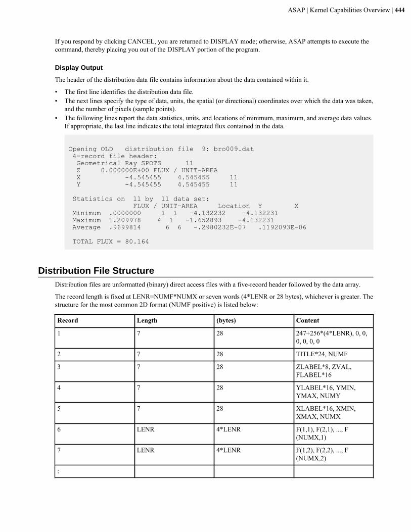
ASAP | Kernel Capabilities Overview | 444
If you respond by clicking CANCEL, you are returned to DISPLAY mode; otherwise, ASAP attempts to execute thecommand, thereby placing you out of the DISPLAY portion of the program.
Display Output
The header of the distribution data file contains information about the data contained within it.
• The first line identifies the distribution data file.• The next lines specify the type of data, units, the spatial (or directional) coordinates over which the data was taken,
and the number of pixels (sample points).• The following lines report the data statistics, units, and locations of minimum, maximum, and average data values.
If appropriate, the last line indicates the total integrated flux contained in the data.
Opening OLD distribution file 9: bro009.dat 4-record file header: Geometrical Ray SPOTS 11 Z 0.000000E+00 FLUX / UNIT-AREA X -4.545455 4.545455 11 Y -4.545455 4.545455 11
Statistics on 11 by 11 data set: FLUX / UNIT-AREA Location Y X Minimum .0000000 1 1 -4.132232 -4.132231 Maximum 1.209978 4 1 -1.652893 -4.132231 Average .9699814 6 6 -.2980232E-07 .1192093E-06
TOTAL FLUX = 80.164
Distribution File StructureDistribution files are unformatted (binary) direct access files with a five-record header followed by the data array.
The record length is fixed at LENR=NUMF*NUMX or seven words (4*LENR or 28 bytes), whichever is greater. Thestructure for the most common 2D format (NUMF positive) is listed below:
Record Length (bytes) Content
1 7 28 247+256*(4*LENR), 0, 0,0, 0, 0, 0
2 7 28 TITLE*24, NUMF
3 7 28 ZLABEL*8, ZVAL,FLABEL*16
4 7 28 YLABEL*16, YMIN,YMAX, NUMY
5 7 28 XLABEL*16, XMIN,XMAX, NUMX
6 LENR 4*LENR F(1,1), F(2,1), ..., F(NUMX,1)
7 LENR 4*LENR F(1,2), F(2,2), ..., F(NUMX,2)
:
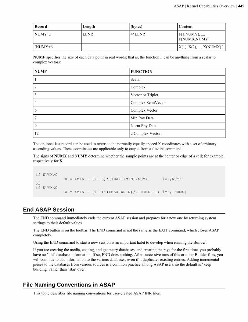
ASAP | Kernel Capabilities Overview | 445
Record Length (bytes) Content
NUMY+5 LENR 4*LENR F(1,NUMY), ...,F(NUMX,NUMY)
[NUMY+6 X(1), X(2), ..., X(NUMX) ]
NUMF specifies the size of each data point in real words; that is, the function F can be anything from a scalar tocomplex vectors:
NUMF FUNCTION
1 Scalar
2 Complex
3 Vector or Triplet
4 Complex SemiVector
6 Complex Vector
7 Min Ray Data
9 Norm Ray Data
12 2 Complex Vectors
The optional last record can be used to override the normally equally spaced X coordinates with a set of arbitraryascending values. These coordinates are applicable only to output from a GRAPH command.
The signs of NUMX and NUMY determine whether the sample points are at the center or edge of a cell; for example,respectively for X:
if NUMX>0 X = XMIN + (i-.5)*(XMAX-XMIN)/NUMX i=1,NUMXor if NUMX<0 X = XMIN + (i-1)*(XMAX-XMIN)/(|NUMX|-1) i=1,|NUMX|
End ASAP SessionThe END command immediately ends the current ASAP session and prepares for a new one by returning systemsettings to their default values.
The END button is on the toolbar. The END command is not the same as the EXIT command, which closes ASAPcompletely.
Using the END command to start a new session is an important habit to develop when running the Builder.
If you are creating the media, coating, and geometry databases, and creating the rays for the first time, you probablyhave no "old" database information. If so, END does nothing. After successive runs of this or other Builder files, youwill continue to add information to the various databases, even if it duplicates existing entries. Adding incrementalpieces to the databases from various sources is a common practice among ASAP users, so the default is "keepbuilding" rather than "start over."
File Naming Conventions in ASAPThis topic describes file naming conventions for user-created ASAP INR files.
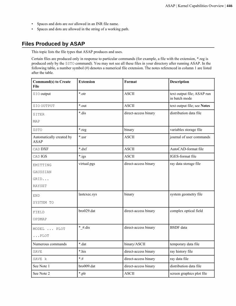
ASAP | Kernel Capabilities Overview | 446
• Spaces and dots are not allowed in an INR file name.• Spaces and dots are allowed in the string of a working path.
Files Produced by ASAPThis topic lists the file types that ASAP produces and uses.
Certain files are produced only in response to particular commands (for example, a file with the extension, *.reg isproduced only by the $STO command). You may not see all these files in your directory after running ASAP. In thefollowing table, a number symbol (#) denotes a numerical file extension. The notes referenced in column 1 are listedafter the table.
Command(s) to CreateFile
Extension Format Description
$IO output *.otr ASCII text output file; ASAP runin batch mode
$IO OUTPUT *.out ASCII text output file; see Notes
$ITER
MAP
*.dis direct-access binary distribution data file
$STO *.reg binary variables storage file
Automatically created byASAP
*.usr ASCII journal of user commands
CAD DXF *.dxf ASCII AutoCAD-format file
CAD IGS *.igs ASCII IGES-format file
EMITTING
GAUSSIAN
GRID...
RAYSET
virtual.pgs direct-access binary ray data storage file
END
SYSTEM TO
lastexec.sys binary system geometry file
FIELD
OPDMAP
bro029.dat direct-access binary complex optical field
MODEL ... PLOT
...PLOT
*_#.dis direct-access binary BSDF data
Numerous commands *.dat binary/ASCII temporary data file
SAVE *.his direct-access binary ray history file
SAVE k *.# direct-access binary ray data file
See Note 1 bro009.dat direct-access binary distribution data file
See Note 2 *.plr ASCII screen graphics plot file
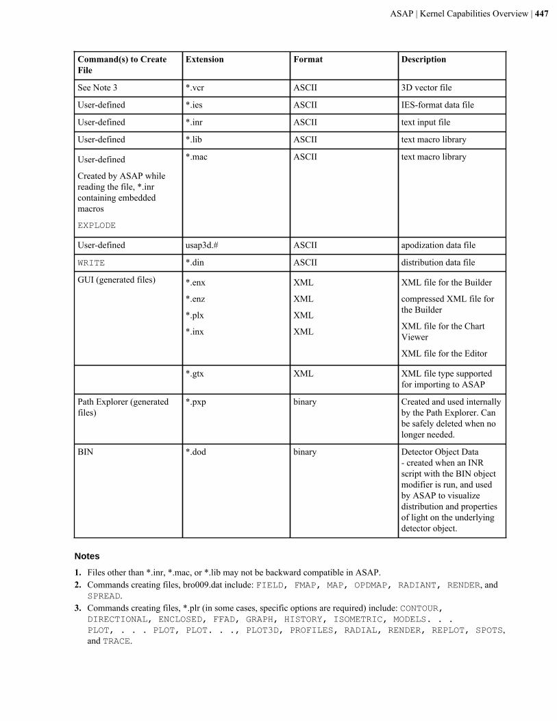
ASAP | Kernel Capabilities Overview | 447
Command(s) to CreateFile
Extension Format Description
See Note 3 *.vcr ASCII 3D vector file
User-defined *.ies ASCII IES-format data file
User-defined *.inr ASCII text input file
User-defined *.lib ASCII text macro library
User-defined
Created by ASAP whilereading the file, *.inrcontaining embeddedmacros
EXPLODE
*.mac ASCII text macro library
User-defined usap3d.# ASCII apodization data file
WRITE *.din ASCII distribution data file
GUI (generated files) *.enx
*.enz
*.plx
*.inx
XML
XML
XML
XML
XML file for the Builder
compressed XML file forthe Builder
XML file for the ChartViewer
XML file for the Editor
*.gtx XML XML file type supportedfor importing to ASAP
Path Explorer (generatedfiles)
*.pxp binary Created and used internallyby the Path Explorer. Canbe safely deleted when nolonger needed.
BIN *.dod binary Detector Object Data- created when an INRscript with the BIN objectmodifier is run, and usedby ASAP to visualizedistribution and propertiesof light on the underlyingdetector object.
Notes
1. Files other than *.inr, *.mac, or *.lib may not be backward compatible in ASAP.2. Commands creating files, bro009.dat include: FIELD, FMAP, MAP, OPDMAP, RADIANT, RENDER, and
SPREAD.3. Commands creating files, *.plr (in some cases, specific options are required) include: CONTOUR,
DIRECTIONAL, ENCLOSED, FFAD, GRAPH, HISTORY, ISOMETRIC, MODELS. . .PLOT, . . . PLOT, PLOT. . ., PLOT3D, PROFILES, RADIAL, RENDER, REPLOT, SPOTS,and TRACE.
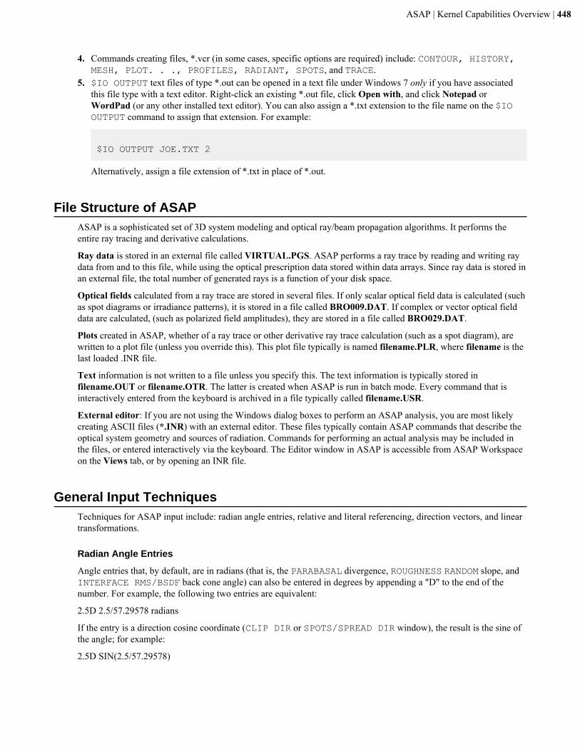
ASAP | Kernel Capabilities Overview | 448
4. Commands creating files, *.vcr (in some cases, specific options are required) include: CONTOUR, HISTORY,MESH, PLOT. . ., PROFILES, RADIANT, SPOTS, and TRACE.
5. $IO OUTPUT text files of type *.out can be opened in a text file under Windows 7 only if you have associatedthis file type with a text editor. Right-click an existing *.out file, click Open with, and click Notepad orWordPad (or any other installed text editor). You can also assign a *.txt extension to the file name on the $IOOUTPUT command to assign that extension. For example:
$IO OUTPUT JOE.TXT 2
Alternatively, assign a file extension of *.txt in place of *.out.
File Structure of ASAPASAP is a sophisticated set of 3D system modeling and optical ray/beam propagation algorithms. It performs theentire ray tracing and derivative calculations.
Ray data is stored in an external file called VIRTUAL.PGS. ASAP performs a ray trace by reading and writing raydata from and to this file, while using the optical prescription data stored within data arrays. Since ray data is stored inan external file, the total number of generated rays is a function of your disk space.
Optical fields calculated from a ray trace are stored in several files. If only scalar optical field data is calculated (suchas spot diagrams or irradiance patterns), it is stored in a file called BRO009.DAT. If complex or vector optical fielddata are calculated, (such as polarized field amplitudes), they are stored in a file called BRO029.DAT.
Plots created in ASAP, whether of a ray trace or other derivative ray trace calculation (such as a spot diagram), arewritten to a plot file (unless you override this). This plot file typically is named filename.PLR, where filename is thelast loaded .INR file.
Text information is not written to a file unless you specify this. The text information is typically stored infilename.OUT or filename.OTR. The latter is created when ASAP is run in batch mode. Every command that isinteractively entered from the keyboard is archived in a file typically called filename.USR.
External editor: If you are not using the Windows dialog boxes to perform an ASAP analysis, you are most likelycreating ASCII files (*.INR) with an external editor. These files typically contain ASAP commands that describe theoptical system geometry and sources of radiation. Commands for performing an actual analysis may be included inthe files, or entered interactively via the keyboard. The Editor window in ASAP is accessible from ASAP Workspaceon the Views tab, or by opening an INR file.
General Input TechniquesTechniques for ASAP input include: radian angle entries, relative and literal referencing, direction vectors, and lineartransformations.
Radian Angle Entries
Angle entries that, by default, are in radians (that is, the PARABASAL divergence, ROUGHNESS RANDOM slope, andINTERFACE RMS/BSDF back cone angle) can also be entered in degrees by appending a "D" to the end of thenumber. For example, the following two entries are equivalent:
2.5D 2.5/57.29578 radians
If the entry is a direction cosine coordinate (CLIP DIR or SPOTS/SPREAD DIR window), the result is the sine ofthe angle; for example:
2.5D SIN(2.5/57.29578)
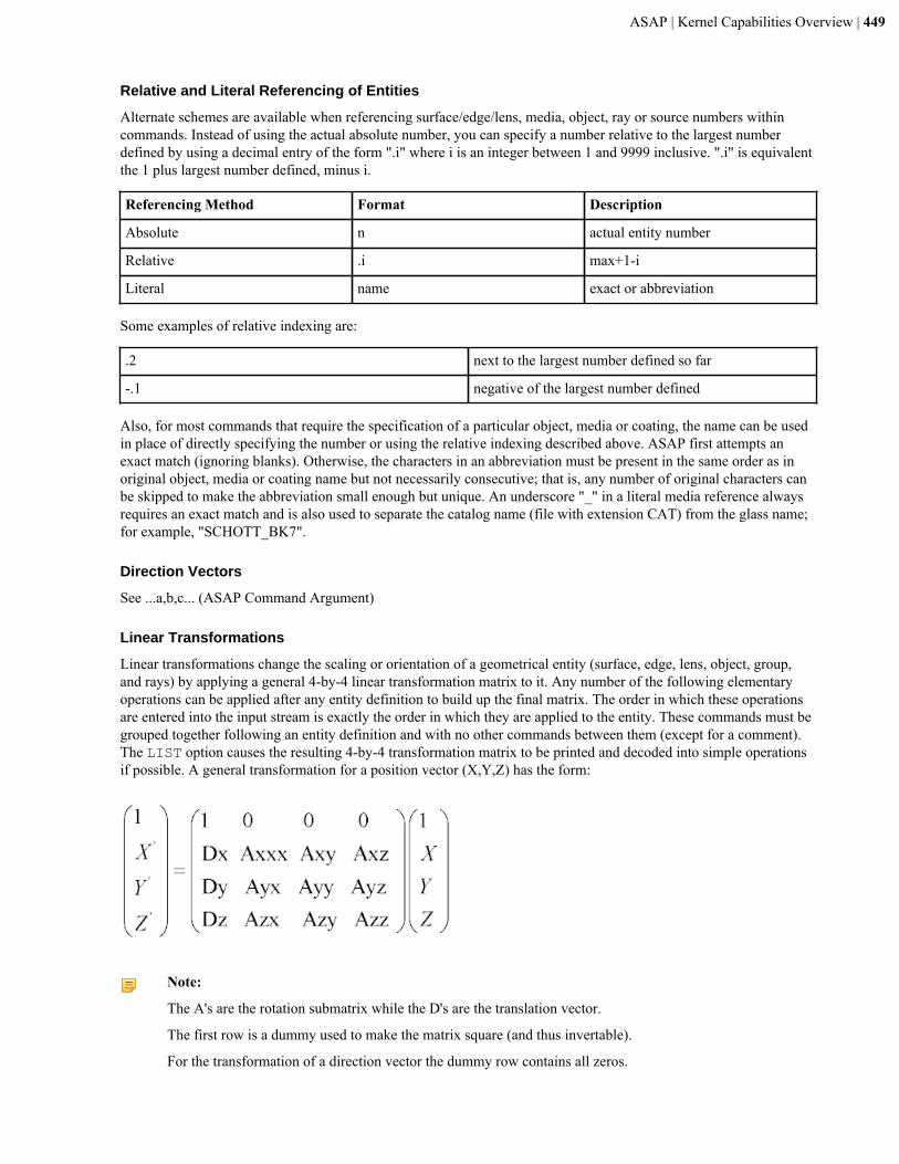
ASAP | Kernel Capabilities Overview | 449
Relative and Literal Referencing of Entities
Alternate schemes are available when referencing surface/edge/lens, media, object, ray or source numbers withincommands. Instead of using the actual absolute number, you can specify a number relative to the largest numberdefined by using a decimal entry of the form ".i" where i is an integer between 1 and 9999 inclusive. ".i" is equivalentthe 1 plus largest number defined, minus i.
Referencing Method Format Description
Absolute n actual entity number
Relative .i max+1-i
Literal name exact or abbreviation
Some examples of relative indexing are:
.2 next to the largest number defined so far
-.1 negative of the largest number defined
Also, for most commands that require the specification of a particular object, media or coating, the name can be usedin place of directly specifying the number or using the relative indexing described above. ASAP first attempts anexact match (ignoring blanks). Otherwise, the characters in an abbreviation must be present in the same order as inoriginal object, media or coating name but not necessarily consecutive; that is, any number of original characters canbe skipped to make the abbreviation small enough but unique. An underscore "_" in a literal media reference alwaysrequires an exact match and is also used to separate the catalog name (file with extension CAT) from the glass name;for example, "SCHOTT_BK7".
Direction Vectors
See ...a,b,c... (ASAP Command Argument)
Linear Transformations
Linear transformations change the scaling or orientation of a geometrical entity (surface, edge, lens, object, group,and rays) by applying a general 4-by-4 linear transformation matrix to it. Any number of the following elementaryoperations can be applied after any entity definition to build up the final matrix. The order in which these operationsare entered into the input stream is exactly the order in which they are applied to the entity. These commands must begrouped together following an entity definition and with no other commands between them (except for a comment).The LIST option causes the resulting 4-by-4 transformation matrix to be printed and decoded into simple operationsif possible. A general transformation for a position vector (X,Y,Z) has the form:
Note:
The A's are the rotation submatrix while the D's are the translation vector.
The first row is a dummy used to make the matrix square (and thus invertable).
For the transformation of a direction vector the dummy row contains all zeros.
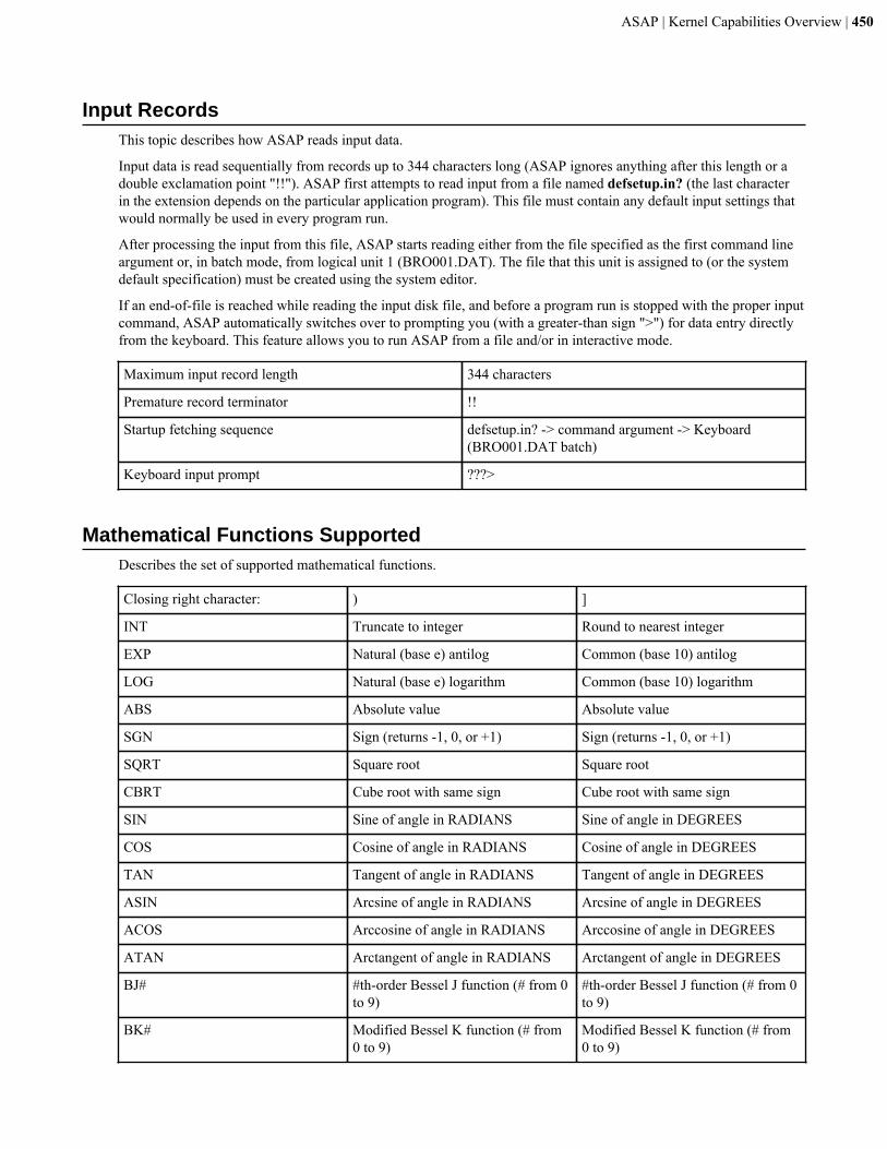
ASAP | Kernel Capabilities Overview | 450
Input RecordsThis topic describes how ASAP reads input data.
Input data is read sequentially from records up to 344 characters long (ASAP ignores anything after this length or adouble exclamation point "!!"). ASAP first attempts to read input from a file named defsetup.in? (the last characterin the extension depends on the particular application program). This file must contain any default input settings thatwould normally be used in every program run.
After processing the input from this file, ASAP starts reading either from the file specified as the first command lineargument or, in batch mode, from logical unit 1 (BRO001.DAT). The file that this unit is assigned to (or the systemdefault specification) must be created using the system editor.
If an end-of-file is reached while reading the input disk file, and before a program run is stopped with the proper inputcommand, ASAP automatically switches over to prompting you (with a greater-than sign ">") for data entry directlyfrom the keyboard. This feature allows you to run ASAP from a file and/or in interactive mode.
Maximum input record length 344 characters
Premature record terminator !!
Startup fetching sequence defsetup.in? -> command argument -> Keyboard(BRO001.DAT batch)
Keyboard input prompt ???>
Mathematical Functions SupportedDescribes the set of supported mathematical functions.
Closing right character: ) ]
INT Truncate to integer Round to nearest integer
EXP Natural (base e) antilog Common (base 10) antilog
LOG Natural (base e) logarithm Common (base 10) logarithm
ABS Absolute value Absolute value
SGN Sign (returns -1, 0, or +1) Sign (returns -1, 0, or +1)
SQRT Square root Square root
CBRT Cube root with same sign Cube root with same sign
SIN Sine of angle in RADIANS Sine of angle in DEGREES
COS Cosine of angle in RADIANS Cosine of angle in DEGREES
TAN Tangent of angle in RADIANS Tangent of angle in DEGREES
ASIN Arcsine of angle in RADIANS Arcsine of angle in DEGREES
ACOS Arccosine of angle in RADIANS Arccosine of angle in DEGREES
ATAN Arctangent of angle in RADIANS Arctangent of angle in DEGREES
BJ# #th-order Bessel J function (# from 0to 9)
#th-order Bessel J function (# from 0to 9)
BK# Modified Bessel K function (# from0 to 9)
Modified Bessel K function (# from0 to 9)

ASAP | Kernel Capabilities Overview | 451
STEP 0 for X<0, 1 for X>0 0 for X<0, 1 for X>0
RECT 0 for |X|>.5, 1 for |X|<.5 0 for |X|>.5, 1 for |X|<.5
GAUS Gaussian EXP(-X^2) Gaussian EXP(-PI*(X^2))
SINC SIN(X)/X SIN(PI*X)/(PI*X)
SOMB 2*BJ1(X)/X 2*BJ1(PI*X)/(PI*X)
FACT X factorial (actually gamma)(|X|+1)with sign of X)
X factorial (actually gamma)(|X|+1)with sign of X)
ERF ERROR function Complement 1-ERF
FILE Next available file number startingat X (usually 10). Blackbody integralfrom 0 to X=microns*degreesK
Next available file number startingat X (usually 10). Blackbody integralfrom 0 to X=microns*degreesK
FBI Fractional Energy Fractional Photons
LPW Lumens per Watt for X degree Kblackbody
Lumens per Watt for X degree Kblackbody
EYE Photopic (bright)
Normalized Visual Response at Xmicrons
Scotopic (dim)
Normalized Visual Response at Xmicrons
LIT Numeric to literal conversion
8 or fewer characters
Numeric to literal conversion
16 or fewer characters
RAN Unit RMS
Symmetric zero-mean randomnumbers of type INT(X) (-15 to 15)
Unit Maximum
Symmetric zero-mean randomnumbers of type INT(X) (-15 to 15)
RAN Type Probability Distribution P(Y) (Max/RMS)^2
-15 Two delta functions 1
-14 |Y| ^14 (14+3) / (14+1)
: : :
-2 |Y| ^2 (2+3) / (2+1)
-1 Ramp 2
0 Uniform 3
1 Cosine 5
2 Convolution of 2 uniforms (triangle) 3*2
: : :
14 Convolution of 14 uniforms 3*14
15 Gaussian 2*LOG(2^32)
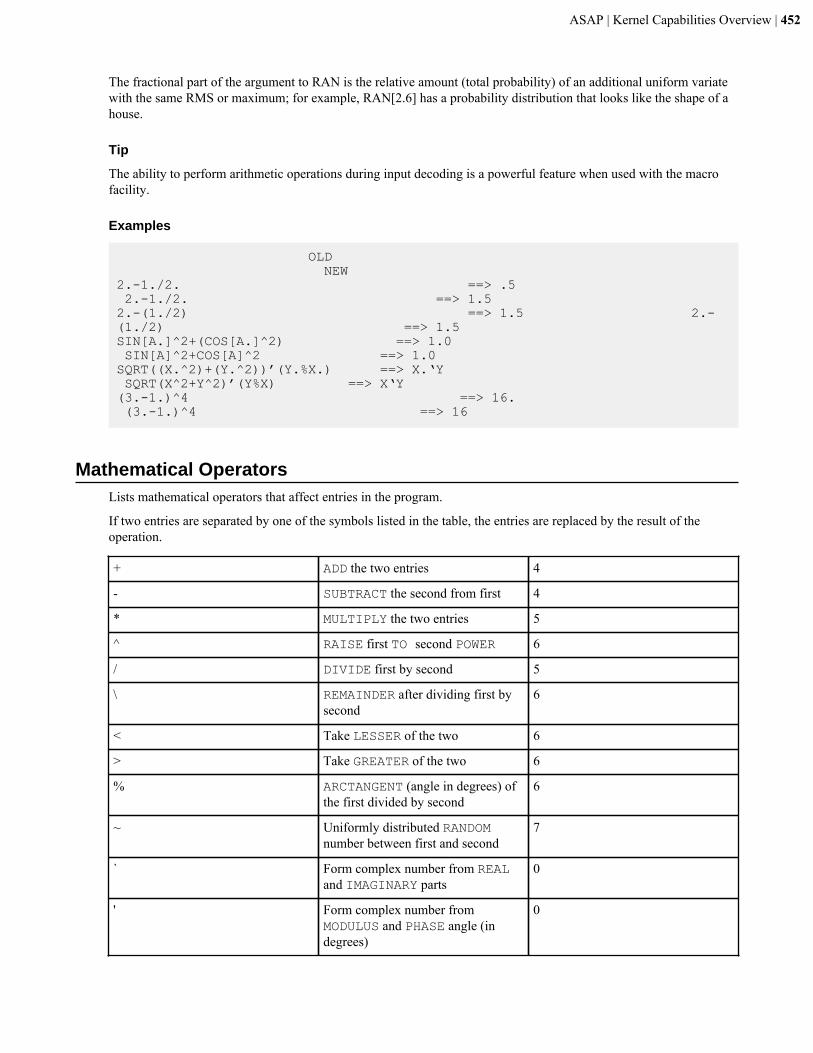
ASAP | Kernel Capabilities Overview | 452
The fractional part of the argument to RAN is the relative amount (total probability) of an additional uniform variatewith the same RMS or maximum; for example, RAN[2.6] has a probability distribution that looks like the shape of ahouse.
Tip
The ability to perform arithmetic operations during input decoding is a powerful feature when used with the macrofacility.
Examples
OLD NEW2.-1./2. ==> .5 2.-1./2. ==> 1.52.-(1./2) ==> 1.5 2.-(1./2) ==> 1.5SIN[A.]^2+(COS[A.]^2) ==> 1.0 SIN[A]^2+COS[A]^2 ==> 1.0SQRT((X.^2)+(Y.^2))’(Y.%X.) ==> X.‘Y SQRT(X^2+Y^2)’(Y%X) ==> X‘Y(3.-1.)^4 ==> 16. (3.-1.)^4 ==> 16
Mathematical OperatorsLists mathematical operators that affect entries in the program.
If two entries are separated by one of the symbols listed in the table, the entries are replaced by the result of theoperation.
+ ADD the two entries 4
- SUBTRACT the second from first 4
* MULTIPLY the two entries 5
^ RAISE first TO second POWER 6
/ DIVIDE first by second 5
\ REMAINDER after dividing first bysecond
6
< Take LESSER of the two 6
> Take GREATER of the two 6
% ARCTANGENT (angle in degrees) ofthe first divided by second
6
~ Uniformly distributed RANDOMnumber between first and second
7
` Form complex number from REALand IMAGINARY parts
0
' Form complex number fromMODULUS and PHASE angle (indegrees)
0
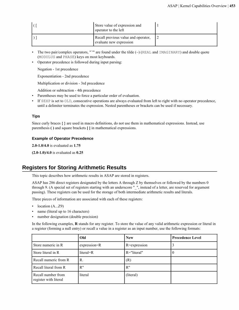
ASAP | Kernel Capabilities Overview | 453
( [ Store value of expression andoperator to the left
1
) ] Recall previous value and operator,evaluate new expression
2
• The two pair/complex operators, "`'" are found under the tilde (~) (REAL and IMAGINARY) and double quote(MODULUS and PHASE) keys on most keyboards.
• Operator precedence is followed during input parsing:
Negation - 1st precedence
Exponentiation - 2nd precedence
Multiplication or division - 3rd precedence
Addition or subtraction - 4th precedence• Parentheses may be used to force a particular order of evaluation.• If $EXP is set to OLD, consecutive operations are always evaluated from left to right with no operator precedence,
until a delimiter terminates the expression. Nested parentheses or brackets can be used if necessary.
Tips
Since curly braces { } are used in macro definitions, do not use them in mathematical expressions. Instead, useparenthesis ( ) and square brackets [ ] in mathematical expressions.
Example of Operator Precedence
2.0-1.0/4.0 is evaluated as 1.75
(2.0-1.0)/4.0 is evaluated as 0.25
Registers for Storing Arithmetic ResultsThis topic describes how arithmetic results in ASAP are stored in registers.
ASAP has 286 direct registers designated by the letters A through Z by themselves or followed by the numbers 0through 9. (A special set of registers starting with an underscore "_", instead of a letter, are reserved for argumentpassing). These registers can be used for the storage of both intermediate arithmetic results and literals.
Three pieces of information are associated with each of these registers:
• location (A...Z9)• name (literal up to 16 characters)• number designation (double precision)
In the following examples, R stands for any register. To store the value of any valid arithmetic expression or literal ina register (forming a null entry) or recall a value in a register as an input number, use the following formats:
Old New Precedence Level
Store numeric in R expression=R R=expression 3
Store literal in R literal=R R="literal" 0
Recall numeric from R R. (R)
Recall literal from R R" R"
Recall number fromregister with literal
literal (literal)
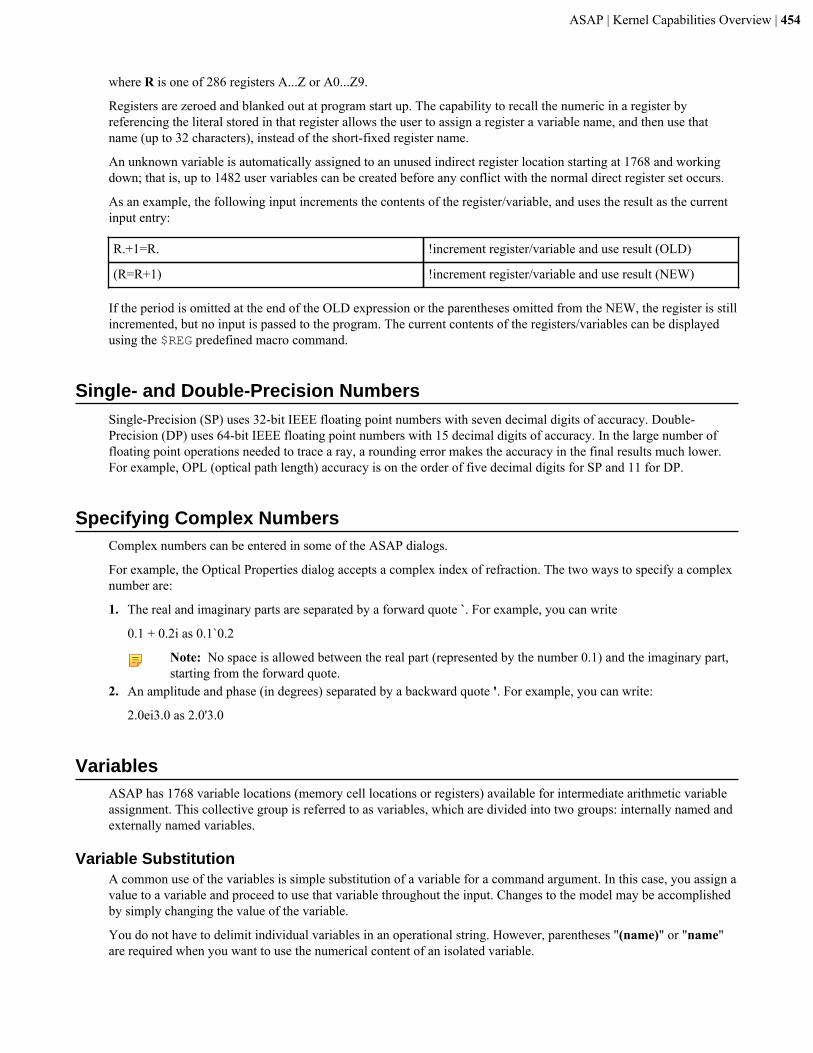
ASAP | Kernel Capabilities Overview | 454
where R is one of 286 registers A...Z or A0...Z9.
Registers are zeroed and blanked out at program start up. The capability to recall the numeric in a register byreferencing the literal stored in that register allows the user to assign a register a variable name, and then use thatname (up to 32 characters), instead of the short-fixed register name.
An unknown variable is automatically assigned to an unused indirect register location starting at 1768 and workingdown; that is, up to 1482 user variables can be created before any conflict with the normal direct register set occurs.
As an example, the following input increments the contents of the register/variable, and uses the result as the currentinput entry:
R.+1=R. !increment register/variable and use result (OLD)
(R=R+1) !increment register/variable and use result (NEW)
If the period is omitted at the end of the OLD expression or the parentheses omitted from the NEW, the register is stillincremented, but no input is passed to the program. The current contents of the registers/variables can be displayedusing the $REG predefined macro command.
Single- and Double-Precision NumbersSingle-Precision (SP) uses 32-bit IEEE floating point numbers with seven decimal digits of accuracy. Double-Precision (DP) uses 64-bit IEEE floating point numbers with 15 decimal digits of accuracy. In the large number offloating point operations needed to trace a ray, a rounding error makes the accuracy in the final results much lower.For example, OPL (optical path length) accuracy is on the order of five decimal digits for SP and 11 for DP.
Specifying Complex NumbersComplex numbers can be entered in some of the ASAP dialogs.
For example, the Optical Properties dialog accepts a complex index of refraction. The two ways to specify a complexnumber are:
1. The real and imaginary parts are separated by a forward quote `. For example, you can write
0.1 + 0.2i as 0.1`0.2
Note: No space is allowed between the real part (represented by the number 0.1) and the imaginary part,starting from the forward quote.
2. An amplitude and phase (in degrees) separated by a backward quote '. For example, you can write:
2.0ei3.0 as 2.0'3.0
VariablesASAP has 1768 variable locations (memory cell locations or registers) available for intermediate arithmetic variableassignment. This collective group is referred to as variables, which are divided into two groups: internally named andexternally named variables.
Variable SubstitutionA common use of the variables is simple substitution of a variable for a command argument. In this case, you assign avalue to a variable and proceed to use that variable throughout the input. Changes to the model may be accomplishedby simply changing the value of the variable.
You do not have to delimit individual variables in an operational string. However, parentheses "(name)" or "name"are required when you want to use the numerical content of an isolated variable.
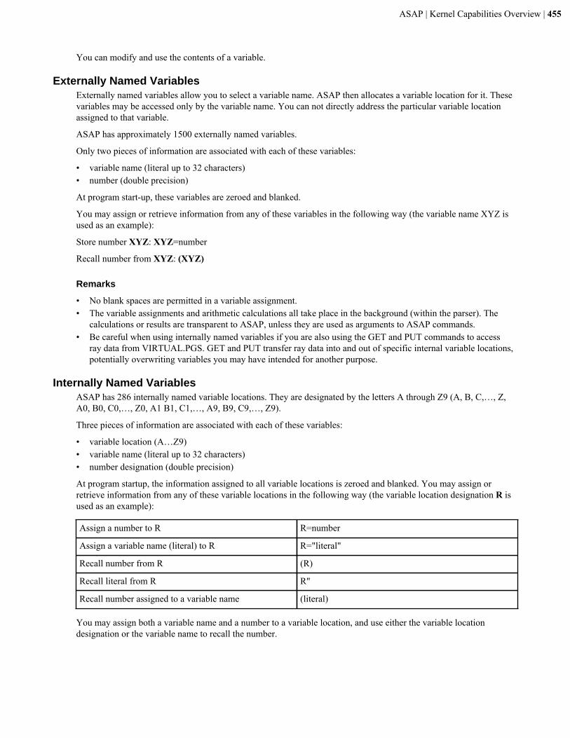
ASAP | Kernel Capabilities Overview | 455
You can modify and use the contents of a variable.
Externally Named VariablesExternally named variables allow you to select a variable name. ASAP then allocates a variable location for it. Thesevariables may be accessed only by the variable name. You can not directly address the particular variable locationassigned to that variable.
ASAP has approximately 1500 externally named variables.
Only two pieces of information are associated with each of these variables:
• variable name (literal up to 32 characters)• number (double precision)
At program start-up, these variables are zeroed and blanked.
You may assign or retrieve information from any of these variables in the following way (the variable name XYZ isused as an example):
Store number XYZ: XYZ=number
Recall number from XYZ: (XYZ)
Remarks
• No blank spaces are permitted in a variable assignment.• The variable assignments and arithmetic calculations all take place in the background (within the parser). The
calculations or results are transparent to ASAP, unless they are used as arguments to ASAP commands.• Be careful when using internally named variables if you are also using the GET and PUT commands to access
ray data from VIRTUAL.PGS. GET and PUT transfer ray data into and out of specific internal variable locations,potentially overwriting variables you may have intended for another purpose.
Internally Named VariablesASAP has 286 internally named variable locations. They are designated by the letters A through Z9 (A, B, C,…, Z,A0, B0, C0,…, Z0, A1 B1, C1,…, A9, B9, C9,…, Z9).
Three pieces of information are associated with each of these variables:
• variable location (A…Z9)• variable name (literal up to 32 characters)• number designation (double precision)
At program startup, the information assigned to all variable locations is zeroed and blanked. You may assign orretrieve information from any of these variable locations in the following way (the variable location designation R isused as an example):
Assign a number to R R=number
Assign a variable name (literal) to R R="literal"
Recall number from R (R)
Recall literal from R R"
Recall number assigned to a variable name (literal)
You may assign both a variable name and a number to a variable location, and use either the variable locationdesignation or the variable name to recall the number.

ASAP | Kernel Capabilities Overview | 456
Tip
The variable name may be used as a literal assignment, without a numerical value, to a variable location. The variablelocation designation may then be used to access the literal.
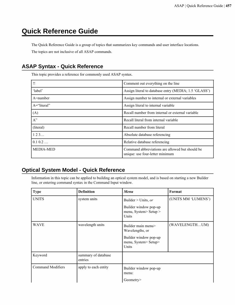
ASAP | Quick Reference Guide | 457
Quick Reference Guide
The Quick Reference Guide is a group of topics that summarizes key commands and user interface locations.
The topics are not inclusive of all ASAP commands.
ASAP Syntax - Quick ReferenceThis topic provides a reference for commonly used ASAP syntax.
!! Comment out everything on the line
‘label’ Assign literal to database entry (MEDIA; 1.5 ‘GLASS’)
A=number Assign number to internal or external variables
A=“literal” Assign literal to internal variable
(A) Recall number from internal or external variable
A” Recall literal from internal variable
(literal) Recall number from literal
1 2 3… Absolute database referencing
0.1 0.2 … Relative database referencing
MEDIA-MED Command abbreviations are allowed but should beunique: use four-letter minimum
Optical System Model - Quick ReferenceInformation in this topic can be applied to building an optical system model, and is based on starting a new Builderline, or entering command syntax in the Command Input window.
Type Definition Menu Format
UNITS system units Builder > Units, or
Builder window pop-upmenu, System> Setup >Units
(UNITS MM ‘LUMENS’)
WAVE wavelength units Builder main menu>Wavelengths, or
Builder window pop-upmenu, System> Setup>Units
(WAVELENGTH…UM)
Keyword summary of databaseentries
Command Modifiers apply to each entity Builder window pop-upmenu:
Geometry>
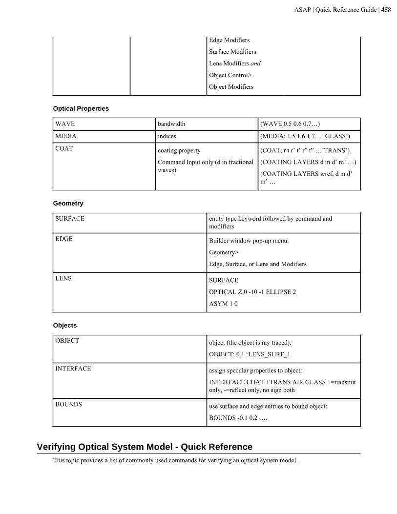
ASAP | Quick Reference Guide | 458
Edge Modifiers
Surface Modifiers
Lens Modifiers and
Object Control>
Object Modifiers
Optical Properties
WAVE bandwidth (WAVE 0.5 0.6 0.7…)
MEDIA indices (MEDIA; 1.5 1.6 1.7… ‘GLASS’)
COAT coating property
Command Input only (d in fractionalwaves)
(COAT; r t r’ t’ r” t” …’TRANS’)
(COATING LAYERS d m d’ m’ …)
(COATING LAYERS wref, d m d’m’ …
Geometry
SURFACE entity type keyword followed by command andmodifiers
EDGE Builder window pop-up menu:
Geometry>
Edge, Surface, or Lens and Modifiers
LENS SURFACE
OPTICAL Z 0 -10 -1 ELLIPSE 2
ASYM 1 0
Objects
OBJECT object (the object is ray traced):
OBJECT; 0.1 ‘LENS_SURF_1
INTERFACE assign specular properties to object:
INTERFACE COAT +TRANS AIR GLASS +=transmitonly, -=reflect only, no sign both
BOUNDS use surface and edge entities to bound object:
BOUNDS -0.1 0.2 ….
Verifying Optical System Model - Quick ReferenceThis topic provides a list of commonly used commands for verifying an optical system model.

ASAP | Quick Reference Guide | 459
Numerical Verification
SHOW display current ASAP settings such as WINDOW,PIXELS, XMEMORY
PRINT print database information
NUMBER N display database numbers and names
Graphical Verification
WINDOW plot window (ASAP autoscales if no values):
WINDOW Y -5 5 Z -10 10
PIXELS profile resolution (does not affect PLOT FACETS):PIXEL 51
PLOT FACETS parametric plot: PLOT FACETS 4 4
PROFILE ray trace plot of system geometry: PROFILE 0 0 -10
$VIEW 3D Viewer (views contents of vector file - use $IOVECTOR REWIND to rewind)
REPLOT replot contents of vector file (shift+left mouse key -curser coordinate; shift+right-click - object numbers)
Source Models - Quick ReferenceThis topic provides a list of commonly used commands for verifying an optical system model.
Incoherent/Coherent Point Source
XMEMORY Set virtual.pgs file to full: XMEMORY FULL
SPECTRUM Spectrally weight sources: SPECTRUM VISUAL
Physical Properties
BEAMS BEAMS COHERENT DIFF
WAVE Wavelength for monochromatic source WAVE 0.5
PARABASAL Parabasal rays (coherent sources only): PARABASAL 4or 8
WIDTHS Parabasal ray modifier (coherent sources only): WIDTH1.6
POLARIZ Polarization ray trace: POLARIZ X 1 0
USERAPOD Flux weighting (spatial/angular): USERAPOD POS/DIR
Spatial Properties
GRID 2d grid coordinates: GRID POLAR …
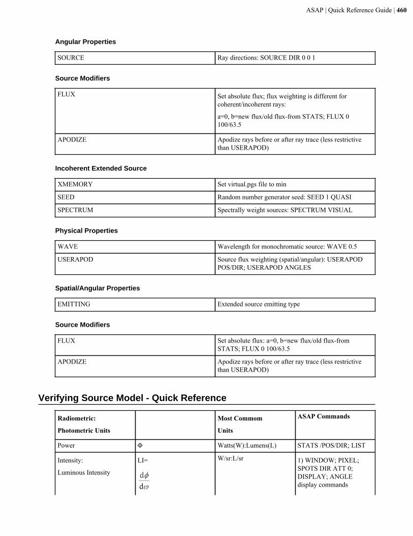
ASAP | Quick Reference Guide | 460
Angular Properties
SOURCE Ray directions: SOURCE DIR 0 0 1
Source Modifiers
FLUX Set absolute flux; flux weighting is different forcoherent/incoherent rays:
a=0, b=new flux/old flux-from STATS; FLUX 0100/63.5
APODIZE Apodize rays before or after ray trace (less restrictivethan USERAPOD)
Incoherent Extended Source
XMEMORY Set virtual.pgs file to min
SEED Random number generator seed: SEED 1 QUASI
SPECTRUM Spectrally weight sources: SPECTRUM VISUAL
Physical Properties
WAVE Wavelength for monochromatic source: WAVE 0.5
USERAPOD Source flux weighting (spatial/angular): USERAPODPOS/DIR; USERAPOD ANGLES
Spatial/Angular Properties
EMITTING Extended source emitting type
Source Modifiers
FLUX Set absolute flux: a=0, b=new flux/old flux-fromSTATS; FLUX 0 100/63.5
APODIZE Apodize rays before or after ray trace (less restrictivethan USERAPOD)
Verifying Source Model - Quick Reference
Radiometric:
Photometric Units
Most Commom
Units
ASAP Commands
Power Φ Watts(W):Lumens(L) STATS /POS/DIR; LIST
Intensity:
Luminous Intensity
LI= W/sr:L/sr 1) WINDOW; PIXEL;SPOTS DIR ATT 0;DISPLAY; ANGLEdisplay commands
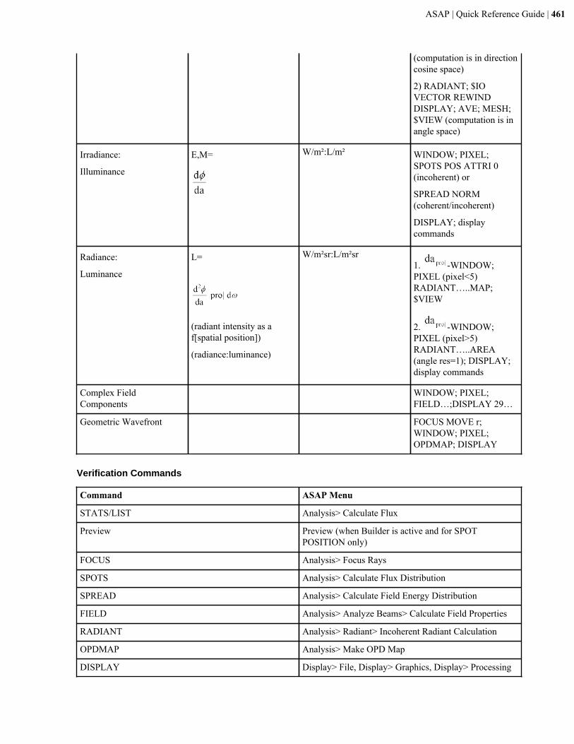
ASAP | Quick Reference Guide | 461
(computation is in directioncosine space)
2) RADIANT; $IOVECTOR REWINDDISPLAY; AVE; MESH;$VIEW (computation is inangle space)
Irradiance:
Illuminance
E,M= W/m²:L/m² WINDOW; PIXEL;SPOTS POS ATTRI 0(incoherent) or
SPREAD NORM(coherent/incoherent)
DISPLAY; displaycommands
Radiance:
Luminance
L=
(radiant intensity as af[spatial position])
(radiance:luminance)
W/m²sr:L/m²sr1. -WINDOW;PIXEL (pixel<5)RADIANT…..MAP;$VIEW
2. -WINDOW;PIXEL (pixel>5)RADIANT…..AREA(angle res=1); DISPLAY;display commands
Complex FieldComponents
WINDOW; PIXEL;FIELD…;DISPLAY 29…
Geometric Wavefront FOCUS MOVE r;WINDOW; PIXEL;OPDMAP; DISPLAY
Verification Commands
Command ASAP Menu
STATS/LIST Analysis> Calculate Flux
Preview Preview (when Builder is active and for SPOTPOSITION only)
FOCUS Analysis> Focus Rays
SPOTS Analysis> Calculate Flux Distribution
SPREAD Analysis> Calculate Field Energy Distribution
FIELD Analysis> Analyze Beams> Calculate Field Properties
RADIANT Analysis> Radiant> Incoherent Radiant Calculation
OPDMAP Analysis> Make OPD Map
DISPLAY Display> File, Display> Graphics, Display> Processing
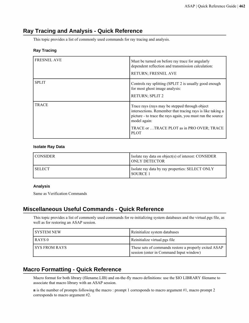
ASAP | Quick Reference Guide | 462
Ray Tracing and Analysis - Quick ReferenceThis topic provides a list of commonly used commands for ray tracing and analysis.
Ray Tracing
FRESNEL AVE Must be turned on before ray trace for angularlydependent reflection and transmission calculation:
RETURN; FRESNEL AVE
SPLIT Controls ray splitting (SPLIT 2 is usually good enoughfor most ghost image analysis:
RETURN; SPLIT 2
TRACE Trace rays (rays may be stepped through objectintersections. Remember that tracing rays is like taking apicture - to trace the rays again, you must run the sourcemodel again:
TRACE or …TRACE PLOT as in PRO OVER; TRACEPLOT
Isolate Ray Data
CONSIDER Isolate ray data on object(s) of interest: CONSIDERONLY DETECTOR
SELECT Isolate ray data by ray properties: SELECT ONLYSOURCE 1
Analysis
Same as Verification Commands
Miscellaneous Useful Commands - Quick ReferenceThis topic provides a list of commonly used commands for re-initializing system databases and the virtual.pgs file, aswell as for restoring an ASAP session.
SYSTEM NEW Reinitialize system databases
RAYS 0 Reinitialize virtual.pgs file
SYS FROM RAYS These sets of commands restore a properly exited ASAPsession (enter in Command Input window)
Macro Formatting - Quick ReferenceMacro format for both library (filename.LIB) and on-the-fly macro definitions: use the $IO LIBRARY filename toassociate that macro library with an ASAP session.
n is the number of prompts following the macro : prompt 1 corresponds to macro argument #1, macro prompt 2corresponds to macro argument #2.
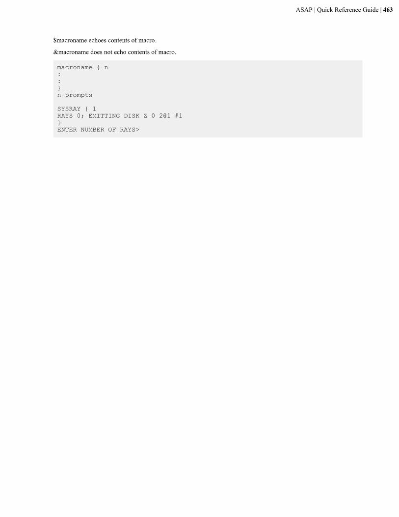
ASAP | Quick Reference Guide | 463
$macroname echoes contents of macro.
¯oname does not echo contents of macro.
macroname { n ::}n prompts
SYSRAY { 1RAYS 0; EMITTING DISK Z 0 2@1 #1}ENTER NUMBER OF RAYS>
ASAP | Index | 464
Index
$ABORT (ASAP Macro) 19$ARGS (ASAP Macro) 32$ASK (ASAP Macro) 37$BEEP (ASAP Macro) 42$CASE (ASAP Macro) 55$CLEAR (ASAP Macro) 64$COPY (ASAP Macro) 79$DATIM (ASAP Macro) 86$DBG (ASAP Macro) 86$DISP (ASAP Macro) 90$DO, begin processing $NEXT 238$DO (ASAP Macro) 93$ECHO (ASAP Macro) 99$EDIT (ASAP Macro) 99$ERR (ASAP Macro) 114$EVAL (ASAP Macro) 115$EXIT (ASAP Macro) 116$EXP (ASAP Macro) 117$FAST (ASAP Macro) 121$FCN, creating piecewise linear curve from 395$FCN (ASAP Macro) 122$FF (ASAP Macro) 123$GO (ASAP Macro) 147$GRAB (ASAP Macro) 148$GUI (ASAP Macro) 157$HELP (ASAP Macro) 168$IF (ASAP Macro) 178$IF THEN (ASAP Macro) 179$IO (ASAP Macro) 187$ITER, begin processing $NEXT 238$ITER (ASAP Macro) 191$LEAVE (ASAP Macro) 198$LOC (ASAP Macro) 205$MENU (ASAP Macro) 222$MSGS (ASAP Macro) 234$NEXT (ASAP Macro) 238$PAGE (ASAP Macro) 249$PATH (ASAP Macro) 253$PLAY (ASAP Macro) 262$PLOT (ASAP Macro) 274$RAN (ASAP Macro) 297$RCL 364$READ (ASAP Macro) 302$REG (ASAP Macro) 304$SCR (ASAP Macro) 332$SEARCH (ASAP Macro) 335$SHOW (ASAP Macro) 346$STAMP (ASAP Macro) 362$STO/$RCL/&STO (ASAP Macro) 364$SYS (ASAP Macro) 368$TIC (ASAP Macro) 377$UNVAR (ASAP Macro) 387$VIEW (ASAP Macro) 404$WAIT (ASAP Macro) 408® 304&SHOW 346&STO 364
&TIC 377
3D focal point 1353D surface map 1343D vector file, replotting data 3083D Viewer, processing system geometry 404
Aa,b,c... (ASAP Command Argument) 15ABEL (ASAP Command) 16ABERRATIONS (ASAP Command) 16ABG (ASAP Command) 18ABSORB (ASAP Command Argument) 20absorption 20ACCURACY (ASAP Command) 20Achieving Optimal Performance in ASAP 13, 419ACTIVITY (ASAP Command Argument) 21add data 31adjacent objects 183AFOCAL (ASAP Command) 22ALIGN (ASAP Command) 23ALLOWED (ASAP Command) 24ALTER (Edge Modifier) (ASAP Command) 25ALTER (Lens Modifier) (ASAP Command) 26ALTER (Surface Modifier) (ASAP Command) 27analysis, isolating rays for 337analysis commands 435ANALYZE (ASAP Command) 28Analyze Ray/Beam Data 435Analyzing the Data 435anamorphic 37ANGLES (ASAP Command) 29ANGLES (ASAP Command Argument) 28anisotropic scatter model, specifying 392apodize, 3D angular volume emitters 389apodize, 3D radiation patterns of volume emitters 391APODIZE (USERAPOD) (ASAP Command) 29, 387APPEND (ASAP Command) 31ARC (ASAP Command) 32arc source 16array, dimensions 89ARRAY (ASAP Command) 33ARRAY NONLINEAR (ASAP Command) 34arrays, numeric 121arrowhead display 36ARROWS (ASAP Command) 36ASAP, end processing 112ASAP files 446ASAP kernel capabilities 440ASAP prompt, return to to 310ASAP REMOTE, commands 157ASAP Syntax - Quick Reference 457ASAP version, printing to command output window 403ASCALE (ASAP Command) 36asphere, superconic 366astigmatism 16
ASAP | Index | 465
ASYM (ASAP Command) 37AutoCAD DXF output file 53auto-correlation length 315AVERAGE (ASAP Command) 38averaging data 137AXICONIC (ASAP Command) 39AXIS, PLOT FACETS option 266axis, setting parameterization for meshing surface 250axis, specifying relative shift 344AXIS (ASAP Command) 40axis of symmetry, creating a plane normal to 260
Bbatch mode, stop ASAP 116beam, coherent sum 131beam, modify data 432beam, move parabasal 232beam data, analyze 435beam data, modify 436beam irradiance, specifying 29, 387beams, creating 429, 431beams, specifying sources 349beams, trace 435beams, tracing a group 433BEAMS (ASAP Command) 42beam set, Gaussian 141beep 42BEND (ASAP Command) 43Bezier 32BEZIER (ASAP Command) 43Bezier edge/curve 76Bezier patches 252biaxial medium, creating 216BIC (ASAP Command) 44BICONIC (ASAP Command) 45BILATERAL (ASAP Command) 46BIN (ASAP Command) 47binary distribution file, create rays from 104BINOMIAL (ASAP Command) 282birefringent, uniaxial crystal 82birefringent coating, create with BIC command 44birefringent media 217boundaries 47bounding, set BSDF 227bounding box, assigning to object 200BOUNDS (ASAP Command) 47box, emitting 103box, plotting wire-frame 269box, spheroid 103boxes, plotting local 269BRANCH (ASAP Command) 48BSDF, SCATTER 331BSDF, set bounding 227BSDFDATA (ASAP Command) 49, 298BSDF interpolation 49BSDF model 28buffer, output 64buffer, replaying current output 262Building the Geometry 420Building Your System 419Bulding the Source 428
CCADEXPORT 88CADEXPORT (ASAP Command) 53calculate, field distribution 125Calculate Diffraction/Propagation Effects 436Cartesian surface 54CARTOVAL (ASAP Command) 54cascaded polarization element 80case, upper and lower 55Cassegrain telescope 371CEC, compound elliptical concentrator 39CHARACTER (ASAP Command) 55character map 93CHC, compound hyperbolic concentrator 39chromatic aberration 16CHROMATICITY (ASAP Command) 56CIE, SOURCE POLYCHROMATIC 350CIE (ASAP Command) 59CIELAB (ASAP Command) 61CIELUV (ASAP Command) 62CIEUVW (ASAP Command) 63circle, sweep 76circular arc 32circular birefringence 21CLIP (ASAP Command) 65CLIP (ASAP Command Argument) 64COARSEN (ASAP Command) 66coating, defining wavelength for 408coatings, creating or modifying 425COATINGS LAYERS (ASAP Command) 67COATINGS MODELS (ASAP Command) 68COATINGS PROPERTIES (ASAP Command) 69coefficients 282coefficients, CONRADY, HERZBERGER, SCHOTT,SELLMEIER 212coefficients, MEDIA command 214coefficients, showing in POLARIZ 345coherent energy distribution, calculating with SPREAD 360coherent Gaussian mode 141COLLECTION (ASAP Command) 70color, reassign 72color, setting 71colorimetry, CHROMATICITY command 56colorimetry analysis 59colorimetry analysis, SET 341COLORS (ASAP Command) 72COLORS (ASAP Command Argument) 71coma 16COMBINE (ASAP Command) 74command, running system 368command arguments, a,b,c 15command arguments, ABSORB 20command arguments, ACTIVITY 21command arguments, ANGLES 28command arguments, CLIP 64command arguments, COLORS 71command arguments, CRYSTAL 82command arguments, GRIN 156command arguments, MINMAX 227command arguments, MODEL 228command arguments, OVERLAY 247
ASAP | Index | 466
command arguments, PIXELS 257command arguments, PLOT 273command arguments, SCATTER 329command arguments, TEXT 374command arguments, XY[Z] 416command categories 419Command Comment Strings 442Command Description Notation 442command entries 442command listing 168command-mode functions 440command prompt return 19command prompt window, opening with $SYS 368commands, examples 441commands, quick reference 457commands, quick reference for optical system model 457commands, quick reference for source models 459commands, quick reference to macro formatting 462commands, quick reference to ray tracing and analysis model 462commands, quick reference to re-initializing and restoring 462commands, quick reference to verifying optical system model 458command scripting 440commands for analysis 435commands for building geometry 420commands for building sources 428commands for tracing rays 432commands for verifying geometry and sources 430Command Usage 441comments, command 442complex numbers, entering in dialogs 454complex vector field 83COMPOSITE (Edge Modifier) (ASAP Command) 74COMPOSITE (Lens Modifier) (ASAP Command) 75computer requirements 13, 419concentrator, compound elliptical, hyperbolic, or parabolic 39conditional block structures 179conditional processing 178CONDUIT (ASAP Command) 76cone, emitting 103Conformal Radiometry, BIN modifier 47CONIC (ASAP Command) 76conic arcs, plotting segments 337conicoid, alter 26conicoid, modify 26conicoid surfaces 340CONRADY media, coefficient 214CONRADY media, creating 212CONSIDER (ASAP Command) 77CONTOUR (ASAP Command) 78coordinate system 40cores, REMOTE processing 157CORNER (ASAP Command) 80corners, rounded for edge 294CPC, compound parabolic concentrator 39CPE (ASAP Command) 80CPU time, displaying 377Create/Modify Media, Coatings, Scatter Models 425Create/Modify Objects 426Create Rays/Beams 429CRYSTAL (ASAP Command Argument) 82crystal media 217cube, axis-aligned 80
curve 32curve, 2D explicit 355curve, 3D general 356curve, creating piecewise linear 395curve, defining in parametric space 398curve, elliptical 100curve, helical 167curve, reversing parametric direction 187curve, smoothing 348curve, sweeping into surface 367curve, uniformly distributed ray set 108curve/edge, placing global position 258curve/edge imaging 180curve/edge points, Bezier surface patches 252curves, platting wireframe 264CUTOFF (ASAP Command) 83CVF (ASAP Command) 83cylindrical 37
Ddata, coordinate axes 46data, creating a table of 371data, emitting 104data, repeating entity 307data, replotting 308data, reset values 377data, smooth 38data, storing or recalling variable 364data, writing to text file 375database, print 285database, storing lens data 364databases, building geometry 420data distribution, display/modify 437data distribution file, dump rays 98data distribution file, sampled 323, 325data file, EULUMDAT 114debug list 86decimal point, U.S. vs. European 441DECOMPOSE (ASAP Command) 86Define/Modify Curve/Edge Entities 421Define/Modify Entities or Single Entity Objects 420Define/Modify Lens Entities 424Define/Modify Surface/Function Entities 422defocus 16DEFORM (ASAP Command) 88depth map 210device type, polarization 185diffraction, calculating effects 436DIFFRACTive surface INTERFACE 95diffuser, MICROSTRUCTURE 223DIMENSIONS (ASAP Command) 89direction, setting for polarization reference ray 278DIRECTIONAL (ASAP Command) 90direction sampling, specifying 379direction vector 15direction vector alignment 23direction vectors 448display, control 99display, distribution data files 443display, valid 241Display/Modify Data Distributions 437
ASAP | Index | 467
DISPLAY (ASAP Command) 91display file header 166distortion 16distribution, 3D representation 223distribution, complex field 125distribution, copying 308distribution data, 3D representation 263distribution data, averaging 137distribution data, clipping 64distribution data, computing encircled energy 294distribution data, creating subset 304distribution data, form of 138distribution data, modify 230distribution data, plotting scale 297distribution data, printing or transferring 335distribution data, producing picture 256distribution data, renormalize 241distribution data, rotating 383distribution data, rotationally average 294distribution data, shifting origin 244distribution data, spatial frequency 124distribution data file, combining 74distribution data file, contour plot 78distribution data file, creating isometric view 190distribution data file, listing functional values of 400distribution data file, polar plot 90distribution data file, profile 148distribution data file, read 91distribution data file, writing to file 412Distribution Data Files Display 443Distribution Data Files Overview 443distribution file, add data 31distribution file, binary 90Distribution File Structure 444DMAP (ASAP Command) 93DOMACROS (ASAP Command) 94DOME (ASAP Command) 95DOPL (ASAP Command) 95DOUBLET (ASAP Command) 96doublet lens, cemented 96doughnut surface, creating 378DRAWING (ASAP Command) 97DUMP (ASAP Command) 98DXF output file 53
Eedge 32edge, convert to curve 66edge, creating 275edge, creating planar 274edge, creating polygonal 247edge, deform or sag 322edge, elliptical 100edge, linearly extend 119edge, modify 25edge, plotting 265edge, sawtooth pattern 326edge/curve, Bezier 43edge/curve, creating rectangular 302edge entities, emitting 107edge or racetrack, creating 294
EDGE points, updating data 387edge-points data 25edges, definitions 99edges, plotting wireframe 265EDGES/CURVES (ASAP Command) 99editor, user-specified 99ELLIPSE (ASAP Command) 100ellipses, plotting polarization state 271ELLIPSOID (ASAP Command) 101elliptical aperture with rectangular grid of rays 150elliptical cross-section, creating a tube 383emit, cone or pyramid 103emit ray set, box or spheroid 103emitter, single-source 102emitter, volume 109EMITTING (ASAP Command) 102EMITTING BOX/SPHEROID (ASAP Command) 103EMITTING CONE/PYRAMID (ASAP Command) 103EMITTING DATA (ASAP Command) 104EMITTING DISK/RECTANGLE (ASAP Command) 106EMITTING ENTITY or OBJECT (ASAP Command) 107EMITTING EULUMDAT (ASAP Command) 108EMITTING FILAMENT (ASAP Command) 108EMITTING HELIX (ASAP Command) 109EMITTING IES (ASAP Command) 110EMITTING OBJECT (ASAP Command) 107EMITTING RAYS (ASAP Command) 111encircled energy 112encircled energy, computing 294ENCLOSED (ASAP Command) 112END (ASAP Command) 112energy density or peak flux, computing 190energy distribution, calculating with SPREAD 360ensquared energy 112entities, define or modify curve/edge 421entities, defining or modifying 420entities, edge 74entities, lens 424entities, surface or function 422ENTITIES (ASAP Command) 113entity, arbitrary scaling 327entity, arbitrary skewing 347entity, edge-based 25entity, lens 75entity, placing relative to 259entity, repeating data 307entity, rotate about a point 314entity, updating storage 387entity/object/source, specifying relative shift along axes 344Entries Repeated and Incremented 442error message, setting 387EULUMDAT, EMITTING 108EULUMDATFILE (ASAP Command) 114example files 441Examples of Command Scripts 441EXPLICIT (ASAP Command) 117explicit entities, defining object 242EXPLODE (ASAP Command) 118EXTEND (ASAP Command) 119EXTREMES (ASAP Command) 119
ASAP | Index | 468
FFACETS (ASAP Command) 121FCN, evaluate 115FDTD Solutions, bidirectional translation with ASAP 83FFAD (ASAP Command) 123FFT (ASAP Command) 124FIELD (ASAP Command) 125FIELDBPM (ASAP Command) 129field curvature 16FIELDSUM (ASAP Command) 131filament, emitting 108files, IES 176files, plots 448files, produced by ASAP 446files, script 448files, searching for paths 335files, setting default path 253files, text 448Files Produced by ASAP 446file structure, distribution 444File Structure of ASAP 448file types 446first-order conditions 28FIT 282FITTED (ASAP Command) 132fitting algorithm, SVD 208FLUX (ASAP Command) 134flux weighting of rays 354FMAP (ASAP Command) 134focus, move rays or beams 233FOCUS (ASAP Command) 135FOLD (ASAP Command) 137FORM (ASAP Command) 138format, FFAD 123form feed 123Fourier transform size 140FRESNEL (ASAP Command) 138FTSIZE (ASAP Command) 140function, assign to medium 220function, wavefront 353FWHM of peak 372
GG2 curvature 355gain option 20GAUSSIAN (ASAP Command) 141Gaussian beam, plotting extent 263Gaussian decomposition 86GENERAL (ASAP Command) 142General Input Techniques 448GENERAL polynomial, assign to medium 220geometrical entities, mixed 113geometries, field propagation 129geometry, four-way plotting 97geometry, plotting 262geometry, rendered graphics of 305geometry, verifying 430GET (ASAP Command) 145glass, creating wedge 409global coordinate, placement 258
global position, curve/edge 258gradient index material 156GRAPH (ASAP Command) 148graphical output, orthogonal or non-orthogonal 243graphical output, setting plotting window 411graphics, creating postscript files 284graphics, plotting 274graphics, plotting curves 264graphics, plotting edges 265graphics, plotting entities 265graphics, plotting facets 266graphics, plotting lenses 268graphics, plotting slices 290graphics, plotting surfaces 272graphics, plotting vectors 272graphics, plotting wire-frame box 269graphics, printing annotated text 374graphics, rendered 305graphics, setting resolution 257graphics, specifying default title 378graphics, terminate mode 310Gregorian telescope 371GRID DATA (ASAP Command) 149GRID ELLIPTIC (ASAP Command) 150GRID HEX (ASAP Command) 151GRID OBJECT (ASAP Command) 152GRID POLAR (ASAP Command) 153GRID RECT (ASAP Command) 154GRID WINDOW (ASAP Command) 155GRIN, create refractive material 218GRIN (ASAP Command Argument) 156GROUP (ASAP Command) 156GUM (ASAP Command) 161
HHALT (ASAP Command) 164HARVEY (ASAP Command) 165Harvey model, create 238header, distribution data files 443HEADER (ASAP Command) 166helical curve, emitting 109HELIX (ASAP Command) 167HERZBERGER media, coefficient 214HERZBERGER media, creating 212hexagonal grid of rays 151HISTOGRAM (ASAP Command) 168HISTORY (ASAP Command) 169HORN (ASAP Command) 173
IIDEAL (ASAP Command) 175IES, ray set creation 110IESFILE (ASAP Command) 176IGES output file 53IMAGE (Global Point) (ASAP Command) 180IMAGE (Ray Positions) (ASAP Command) 181image aberrations 16IMAGE Curve/Edge (ASAP Command) 180imaging a global point 180IMMERSE (ASAP Command) 181
ASAP | Index | 469
IMPORT (ASAP Command) 182importance area, specifying 379incoherent energy distribution, calculating with SPREAD 360inhomogeneous media, field propagation 129inhomogeneous scattering, Monte Carlo 329input/output, controlling redirection 187Input Records 450input records, iterating 191intensity apodization, specifying 29, 387interface, assigning characteristics 186interface, assigning near-specular scattering 331INTERFACE (ASAP Command) 183INTERFACE (Polarization Modifiers) (ASAP Command) 185INTERFACE REPEAT (ASAP Command) 186intersection, setting local and global for object 333INVERT (ASAP Command) 187irradiance, flux-per-unit for 3D array 405IRRADIANCE (ASAP Command) 190ISOMETRIC (ASAP Command) 190isotropic scatter model, ABg 18isotropic scatter model, K-Correlation 194isotropic scatter model, specifying 392
JJONES (ASAP Command) 193Jones vector form 204
KKCORRELATION (ASAP Command) 194K-Correlation scatter model 194Kernel Capabilities Overview 440keystone 36
LLAMBERTIAN (ASAP Command) 195layers, coating 67LCC (ASAP Command) 195lens, conicoid surfaces 340lens, doublet 96lens, Mangin 209lens, plotting 265, 268lens, realistic 255lens, simple singlet 346lens, storing current state 364lens, varying construction parameters during optimization 401lens conicoid, explode 118lens conicoid database 26LENS conicoids, updating data 387lens entities, explode 118lens entity, imaging global point through 180lenses, defining 198lenses, searching for rays within 310LENSES (ASAP Command) 198lens modifier 26LEVEL (ASAP Command) 199LIGHTS (ASAP Command) 200light sources, setting optional 200LIMITS (ASAP Command) 200
LINE (ASAP Command) 202linear curve, piecewise 66linear shift invariant 165linear shift invariant, scatter model 18linear transformation, specifying application of 414linear transformations 448line edge, creating 202LIST (ASAP Command) 202LIST (Parabasal Ray Data) (ASAP Command) 204LIST ELLIPSE (ASAP Command) 203LIST INTEGER (ASAP Command) 204LIST RAYS (ASAP Command) 204LIST with SCALE 327literals, grabbing 148LM-63-1995 IESNA file 176LOCAL, Cartesian coordinate 40LOCAL (ASAP Command) 206local bounding box 206looping input records 93LSQFIT (ASAP Command) 208
MMacro Formatting - Quick Reference 462macros, $GUI 157macros, $HELP 168macros, $IO 187macros, $NEXT 238macros, $PAGE 249macros, $PATH 253macros, $PLAY 262macros, $PLOT 274macros, $RAN 297macros, $READ 302macros, $REG 304macros, $SEARCH 335macros, $SHOW 346macros, $STO, $RCL, &STO 364macros, $SYS 368macros, $TIC 377macros, $WAIT 408macros, argument prompts 32macros, beeping 42macros, binary distribution file 90macros, branching or skipping 147macros, call editor 99macros, case 55macros, clear buffer 64macros, control 94macros, control display 99macros, copy source file 79macros, creating block of records or structures 178macros, date and time stamp 86macros, debug 86macros, display currently defined 222macros, displaying status of 346macros, evaluate function 115macros, exit before completing 198macros, expression precedence 117macros, fast reading 121macros, form feed 123macros, grabbing numbers or literals 148
ASAP | Index | 470
macros, interate input records 191macros, local register/variable names 205macros, looping 93macros, math function 122macros, message display 234macros, processing conditional block structures 179macros, screen template 332macros, skip records 114macros, stop loop 19macros, stops ASAP in batch mode 116macros, variable value 37MANGIN (ASAP Command) 209map, contour 134map, geometric wavefront 244MAP (ASAP Command) 210material, create absorbing refractive 215material, create single refractive 212Mathematical Functions Supported 450Mathematical Operators 452math function, define inline 122matrices, creating ABCD and Jones 175matrix 33MATRIX (ASAP Command) 211matrix element, Jones 193media, creating or modifying 425media, define birefringent 217media, defining wavelength for 408MEDIA (ASAP Command) 212MEDIA ABSORB (ASAP Command) 215MEDIA BIAXIAL (ASAP Command) 216media coefficients, CONRADY, HERZBERGER, SCHOTT,SELLMEIER 214MEDIA Command Coefficients 214MEDIA CRYSTAL (ASAP Command) 217MEDIA GRIN (ASAP Command) 218median 38MEDIA SCATTER (ASAP Command) 220MEDIA USER (ASAP Command) 221medium, assign GENERAL polynomial 220memory cell locations 454mesh, plotting 270MESH (ASAP Command) 223meshing, parameterization 250mesh patches, subdividing 121messages, display of 234messages, output of parent ray warning 408messages, setting type 387MICROSTRUCTURE, PLOT FACETS option 266MICROSTRUCTURE (ASAP Command) 223MIE 251MINIMIZE (ASAP Command) 225MINMAX (ASAP Command Argument) 227mirror, create Mangin 209MIRROR (ASAP Command) 227Miscellaneous Useful Commands - Quick Reference 462MISSED (ASAP Command) 228mixed geometrical entities 113model, create scattering 229model, creating composite scatter 365model, plotting 273model, reflection 256model, scatter 329
MODEL (ASAP Command Argument) 228modeling of physical optics in ASAP 440models, coatings 68MODELS (ASAP Command) 229modifier, edge, 25MODIFY (ASAP Command) 230Modify or Use Internal Ray/Beam Data as Input 436Modify Ray/Beam Data 432MONTECARLO 356Monte Carlo, inhomogeneous scattering 329MOVE (ASAP Command) 231MOVE PARABASALS (ASAP Command) 232MOVE TO FOCI (ASAP Command) 233MOVE TO PLANE (ASAP Command) 233MOVE TO POINT (ASAP Command) 233MOVE TO SPHERE (ASAP Command) 234MUELLER (ASAP Command) 234MULTIPLE (ASAP Command) 236multiple surfaces or edges, creating solid or mesh object 242
NNONLINEAR (ASAP Command) 238nonlinearly spaced surfaces 34non-orthogonal graphical output 243NORMALIZE (ASAP Command) 241number, seed 336numbers, grabbing 148NUMBERS (ASAP Command) 241
Oobject, adding options 303object, assigning near-specular scatter interface 331object, assigning roughness 315object, assigning scatter interface to an 329object, assigning scatter repeat characteristics 331object, avoid 24object, collection of 156object, defined in parametric space 398object, defining or modifying single entity 420object, deformations 88object, display name tree 383object, faceting and viewing shortcut 406object, global bounding box 200object, INTERFACE polarization 185object, lens-based 16object, rotate about a point 314object, setting intersection strategy 333object, skip 24object, uniform grid of rays 152OBJECT (ASAP Command) 242Object Creation 428object interface, assigning 183object name, branch 48objects, choosing 77objects, creating 428objects, creating or modifying 426objects, emitting 107objects, plotting parametric mesh 266objects, plotting slices 290objects, plotting with wireframe 270
ASAP | Index | 471
objects in contact 183OBLIQUE (ASAP Command) 243OFFSET (ASAP Command) 244OPDMAP (ASAP Command) 244OPTICAL (ASAP Command) 245optical element, creating 175optical-mechanical system modeling in ASAP 440optical path length, controls 95optical properties, building 420Optical System Model - Quick Reference 457optimization, declaring lens construction parameters for 401orthogonal graphical output 243output, pausing text 249OVAL (ASAP Command) 247OVERLAY (ASAP Command Argument) 247
PPARABASAL (ASAP Command) 249parabasal ray data, list 204parabasal rays 233parabasal rays, modifying settings 410parabolic curve, bend 43parallel surfaces 236PARAMETERIZE (ASAP Command) 250parametric coordinate of curve/edge 258parametric direction, reversing 187parametric mesh, plotting 266paraxial departure violation 405PARTICLES (ASAP Command) 251particulate scatter model 251patches, mesh 121PATCHES (ASAP Command) 252paths, searching 335PATHS (ASAP Command) 253pattern 33pause ASAP before continuing 408pcname 157peak, printing number of 372peen 33peens, MICROSTRUCTURE 223PENTA (ASAP Command) 312PERFECT (ASAP Command) 255Phong model, create 238photometry IES files 110PHYSICAL (ASAP Command) 256PICTURE (ASAP Command) 256pixels, averaging 38PIXELS, HISTORY, OVERLAY, PLOT, PROFILES, SPOTS,XY[Z] 262PIXELS (ASAP Command) 257PIXELS (ASAP Command Argument) 257PLACE (CURVE/EDGE) (ASAP Command) 258PLACE (Global Coordinate) (ASAP Command) 258PLACE (Relative to Entity) (ASAP Command) 259placement, absolute 258planar edge, creating 274plane, creating sawtooth pattern 326plane, move rays to 233PLANE (ASAP Command) 260PLANE NORMAL (ASAP Command) 261PLANE POINTS (ASAP Command) 261
plot, contour 78plot, setting number of pixels 257plot, setting window for output 411PLOT (ASAP Command Argument) 273PLOT3D (ASAP Command) 263PLOT BEAMS (ASAP Command) 263PLOT CURVES (ASAP Command) 264PLOT EDGES (ASAP Command) 265PLOT ENTITIES (ASAP Command) 265PLOT FACETS (ASAP Command) 266PLOT LENSES (ASAP Command) 268PLOT LIMITS (ASAP Command) 269PLOT LOCAL (ASAP Command) 269PLOT MESHES (ASAP Command) 270plot of data values 168plot options, standard 431PLOT POLARIZATION (ASAP Command) 271PLOT RAYS (ASAP Command) 272plots, date and time stamp 86plots, overlaying 247plots, setting up 430plots, true perspective view 403plots from calculations 443PLOT SURFACES (ASAP Command) 272Plotting Commands 262plotting distribution data 138plotting geometry 97plotting segments segments 337plot window, temporary override 416point, move rays to 233point, rotate about 314points, axis for fixed direction 190points, creating a plane 261POINTS (2D) (ASAP Command) 274POINTS (3D) (ASAP Command) 275polar, circular grid 153POLARIZ, showing complex coefficients 345POLARIZ (ASAP Command) 277POLARIZ (Polarization Vector) (ASAP Command) 279POLARIZ (Randomized) (ASAP Command) 280POLARIZ (Reference Coordinate) (ASAP Command) 281polarization, BIAXIAL MEDIA 216polarization, cascading polarization element (CPE) 80polarization, create birefringent coating 44polarization, device type 185polarization, DUMP 98polarization, general uniaxial media (GUM) models 161polarization, interface modifiers 185polarization, JONES matrix element 193polarization, liquid crystal cell device (LCC) 195polarization, list states 204polarization, MUELLER matrix elements 234polarization, reference coordinate 281polarization, setting properties 277polarization, setting the mode 279polarization, surface modifiers 289polarization, vector 279polarization parameters, lists 203polarization state ellipses, plotting 271polarizer, realistic model 318POLARIZ K (Reference Ray Direction) (ASAP Command) 278POLARIZ MODE (ASAP Command) 279
ASAP | Index | 472
POLYCHROMATIC, SELECT 337POLYCHROMATIC, SOURCE 350polygonal edge, creating 247polynomial, best fit 305polynomial, renormalize coefficients 306POLYNOMIAL/TRINOMIAL/BINOMIAL (ASAP Command)282polynomial coefficients 27polynomial coefficients, creating scatter model with 282positivity violation 405PostScript File Utility (PSCRIP) (ASAP Command) 284print, annotated text 374PRINT (ASAP Command) 285PRINT MODEL (Polarization) (ASAP Command) 289prism, creating 312profile, graph 148PROFILES (ASAP Command) 290projection, graphical output 243propagation, calculating effects 436propagation, field 129propagation, reverse direction 310propagation paths of rays 253properties, coatings 69PSCRIP utility, creating postscript files 284PUT (ASAP Command) 291pyramid, emitting 103
Qquick commands, quick reference for syntax 457Quick Reference Guide 457
RRACETRACK (ASAP Command) 294RADIAL (ASAP Command) 294radial profile, creating surface with 397radian angle entries 448RADIANCE 29RADIANT (ASAP Command) 295radiant intensity distribution 29random, scatter 329randomized polarization 280random number generator, initializing seed 336random number seed, resetting 297RANGE (ASAP Command) 297RAN type 450RAWDATA (ASAP Command) 298ray, defining and tracing 298ray, flux weighting 354ray, limiting or clipping box 65ray, modify data 432ray, modify flux 134ray, move parabasal 232ray, move to plane 233ray, move to point 233ray, move to sphere 234ray, plot missed 228ray, plotting vector 272ray, polarization properties 277ray, reverse propagation direction 310ray, searching within lenses 310
ray, setting beam shape 342ray, setting total number of 300ray, specifying arbitrary set 300ray, specifying propagation direction 353ray, specifying sources 349ray, splitting 356ray, summary of propagation path 253ray, termination 83ray, trace 435ray, tracing selected 381ray, types of tracing data saved 434ray, warning messages 408RAY (ASAP Command) 298ray control 24ray creation, defaults 42ray data, 3D focal point 135ray data, analyze 435ray data, calculating intensity or radiance 295ray data, copying variable data to 291ray data, creating map 244ray data, display/modify 437ray data, formatting for FFAD 123ray data, geometric spot diagram for 358ray data, list 202ray data, list in EMITTING RAYS format 204ray data, listing statistics 363ray data, list polarization parameters 203ray data, minimum and maximum 119ray data, modify 436ray data, plotting 262, 262ray data, recalling 169ray data, retrieving and copying 145ray data, specifying type and amount to store 414ray data, stored in VIRTUAL.PGS 435ray database, list 204ray fluxes, modify 134ray grid, rectangular raster 155Ray matrix 175ray modifier 181ray polarization state, dumping 98rays, create arbitrary set 111rays, creating 429rays, creating in media 181rays, distribute randomly 107rays, dumping to file 98rays, emitting 111rays, grid or collection of 428rays, hexagonal grid 151rays, move 231rays, rectangular grid 149, 150rays, setting parabasal 249rays, termination 164rays, tracing 432rays, tracing a group 433rays, uniform grid on an object 152RAYS (ASAP Command) 300ray set, efficiency or flux 70ray set, emitting 103, 104, 108, 110ray set, isolating for analysis 337ray set, list parabasal ray data 204ray set, selecting subset 365rayset, setting beam shape 342
ASAP | Index | 473
RAYSET (ASAP Command) 300ray trace, Fresnel adjustment 138ray trace, setting up 433, 435ray trace, write data 326ray trace accuracy versus speed 20ray trace data 40Ray Tracing and Analysis - Quick Reference 462ray tracing data, saving 434reading input data 450realistic, model-based polarizer 318realistic, retarder model 319records, branching or skipping 147records, reading 302records, skip 114RECTANGLE (ASAP Command) 302rectangles, hinging 314rectangular cross-section, creating a tube 383rectangular edge 294rectangular edge or curve, creating rounded-corner 317rectangular grid of rays 149, 154REDEFINE (ASAP Command) 303redirecting input/output 187REDUCE (ASAP Command) 304reference coordinate, polarization 281reflection/transmission coefficients, adjusting with Fresnel 138refractive, create absorbing material 215refractive, create GRIN material 218refractive, create single material 212refractive element 95register locations 454registers, displaying 304registers, storing arithmetic results in 453registers/variables, local 205Registers for Storing Arithmetic Results 453relative and literal referencing 448REMOTE commands with $GUI 157REMOVE (ASAP Command) 305RENDER, setting light sources 200RENDER (ASAP Command) 305RENORM (ASAP Command) 306REPEAT, SCATTER 331REPEAT (ASAP Command) 307repetitive 33replay current output buffer 262REPLICATE (ASAP Command) 308REPLOT (ASAP Command) 308RESET (ASAP Command) 309resolution, setting for graphics 257RESTRICT (ASAP Command) 310RETURN (ASAP Command) 310REVERSE (ASAP Command) 310REVOLUTION (ASAP Command) 311REVOLUTION (Fitted) (ASAP Command) 311RGB values 71, 72RIGHT (ASAP Command) 312RMS, SCATTER 331RMS (ASAP Command) 313RMS spot size 16RMS spot size, minimize 225ROOF (ASAP Command) 314ROTATE (ASAP Command) 314rotating distribution data 383
ROUGHNESS (ASAP Command) 315ROUNDED (ASAP Command) 317RPM (ASAP Command) 318RRM (ASAP Command) 319
SSAG (ASAP Command) 322SAMPLED (ASAP Command) 323SAMPLED (Cylindrical) (ASAP Command) 325SAVE (ASAP Command) 326saving system data 369SAWTOOTH (ASAP Command) 326scale 36SCALE (ASAP Command) 327SCALE FROM (ASAP Command) 328SCATTER (ASAP Command Argument) 329scattered rays, rescattering 199scattering, anisotropic surfaces 228scattering, microstructure 223scattering model, create 229scatter model 313scatter model, ABG command 18scatter model, anisotropic 400scatter model, combing Phong and Harvey 238scatter model, creating 282scatter model, creating composite 365scatter model, creating particulate 251scatter model, Harvey 165scatter model, isotropic or anisotropic 392scatter model, K-Correlation 194scatter model, Lambertian 195scatter model, particulate 251SCATTER MODEL, using TOWARDS 379scatter model, v-cavities 402SCATTER MODEL (ASAP Command) 329scatter models, creating or modifying 425SCATTER RANDOM (ASAP Command) 329SCATTER REPEAT (ASAP Command) 331SCATTER RMS/BSDF (ASAP Command) 331SCHOTT media, coefficient 214SCHOTT media, creating 212SCR editor 32screen template, user-programmable 332scripts, examples 441SEARCH (ASAP Command) 333SECTION (ASAP Command) 335SEED (ASAP Command) 336SEGMENTS (ASAP Command) 337Seidel 16SELECT (ASAP Command) 337SELLMEIER media, coefficient 214SELLMEIER media, creating 212SEQUENCE (ASAP Command) 340SET (ASAP Command) 341settings, reinitialize control 309Setting the Working Directory 14, 420Setup Beam Creation 431Setup Plots and Verify System 430Setup Trace 433SHAPE (ASAP Command) 342SHIFT (ASAP Command) 344
ASAP | Index | 474
SHOW (ASAP Command) 345simple mirror, create 227SINGLET (ASAP Command) 346singlet lens, creating simple 346singular value decomposition 208SKEW (ASAP Command) 347skewing an entity/object/source 347smooth, data 38SMOOTH (ASAP Command) 348SOLID (ASAP Command) 348solid-state drive (SSD) 13, 419solid surface 348source, building 428source, collection of 156source, rotate about a point 314SOURCE (ASAP Command) 349source file, copy 79Source Models - Quick Reference 459SOURCE POLYCHROMATIC (ASAP Command) 350sources, memory usage 13, 419sources, verifying 430SOURCE WAVEFUNC (ASAP Command) 353space and color difference, calculating 61, 62, 63spatial frequency 124Specifying Complex Numbers 454spectral apodization, flux weighting of rays 354SPECTRUM (ASAP Command) 354specular components, splitting rays into 356sphere, move rays to 234spherical aberration 16SPLINE, EXPLICIT 2D (ASAP Command) 355SPLINE, GENERAL 3D (ASAP Command) 356SPLIT (ASAP Command) 356spot diagram, creating geometric 358SPOTS (ASAP Command) 358SPREAD (ASAP Command) 360Standard Plot Options 431startup settings, reset 309statistics, listing for ray data 363statistics, printing for TRACE 363STATS (ASAP Command) 363STATS TRACE (ASAP Command) 363Stokes vector form 204stop processing 112STORE (ASAP Command) 364string, character 55strings, alpha-numeric 441SUBSET (ASAP Command) 365SUM (ASAP Command) 365summing, coherent beams 131SUPERCONIC (ASAP Command) 366surface 39, 43surface, biconic 45surface, Cartesian 54surface, conicoid 340surface, convert function to explicit 117surface, creating a plane 261surface, creating aspheric 245surface, creating with user-defined function 396surface, creating with user-defined radial or toric profile 397surface, cylindrical or anamorphic 37surface, deformed cylindrical 325
surface, deforming edge or sag onto 322surface, ellipsoidal 101surface, explicit 323surface, fitting points 132surface, general 142surface, general transformation matrix 211surface, linearly spaced 33surface, making solid 348surface, multiple parallel 236surface, plot local boxes 269surface, plotting 265surface, polarization modifiers for 289surface, rotating 2D curve 311surface, rotating 2D curve fit 311surface, selecting branch for test point or direction 373surface, setting parameterization for meshing 250surface, signaling definition commands 367surface, specifying explicit Zernike polynomial 416surface, sweeping curve into 367surface, toroidal or doughnut 378surface/function, local bounding box 206surface/function polynomials, renormalizing 306SURFACE coefficients, updating 387surface entities, emitting 107surface mesh, Bezier patches 252surface modifier 27surfaces, depth map 210surfaces, emitting 106surfaces, plotting 272surfaces, rough 256surfaces, scattering from anisotropic 228SURFACES/FUNCTIONS (ASAP Command) 367SVD 282SWEEP (ASAP Command) 367syntax, command 442system, define units 386system, verifying 430SYSTEM (ASAP Command) 369system geometry, plotting 262system information, storing and retrieving 369system-wide parameter, SET 341
TTABLE (ASAP Command) 371TELESCOPE (ASAP Command) 371telescope element 22templates, command scripts 441TERRAIN (ASAP Command) 372TEST (ASAP Command) 373TEXT (ASAP Command Argument) 374TEXTFILE (ASAP Command) 375THRESHOLD (ASAP Command) 377timestamp, $STAMP 362TIR (Total Internal Reflection) 379TITLE (ASAP Command) 378toric profile, creating surface with 397toroidal surface, creating 378TORUS (ASAP Command) 378TOWARDS (ASAP Command) 379TRACE, printing statistics of 363TRACE (ASAP Command) 381
ASAP | Index | 475
Trace Ray and Beams 435Tracing a Group of Rays or Beams 433tracing rays in ASAP 440Tracing the Rays 432transform, Abel 16transformation matrix 211, 327TRANSPOSE (ASAP Command) 383TREE (ASAP Command) 383TRINOMIAL (ASAP Command) 282tube, creating generalized tube 173TUBE (ASAP Command) 383Types of Ray Tracing Data Saved by ASAP 434
UUNITS 408units, defining system 386units, scaling 328UNITS (ASAP Command) 386UPDATE (ASAP Command) 387USERAPOD (ASAP Command) 29, 387USERAPOD ANGLES (ASAP Command) 389USERAPOD BOTH (ASAP Command) 391USERBSDF (ASAP Command) 392USERCURVE (ASAP Command) 395USERFUNC (ASAP Command) 396user interface commands 157USERSAG (ASAP Command) 397USERSCAT, subroutine 221UVSPACE (ASAP Command) 398
Vvalley, printing number of 372VALUES (ASAP Command) 400VANES (ASAP Command) 400variable data, storing or recalling 364Variables 454variables, printing or transferring distribution data 335VARIABLES (ASAP Command) 401variable value 37VCAVITY (ASAP Command) 402vector, polarization 279vector, randomized polarization state vector 280vector file, creating 3D representation in 223vector file, system geometry 404vector form, Jones and Stokes 98vectors, plotting 272Verifying Optical System Model - Quick Reference 458Verifying the Geometry and Sources 430VERSION (ASAP Command) 403VIEW (ASAP Command) 403VIOLATION (ASAP Command) 405virtual.pgs file 13, 419virtual memory paging, setting number of rays 300VOLUME 251volume, flux-per-unit for 3D array 405volume emitters, apodizing 391volume emitters, specifying 3D angular apodization 389volume scattering, MEDIA USER 221VOXELS (ASAP Command) 405VUFACETS (ASAP Command) 406
Wwarning message, setting 387WARNINGS (ASAP Command) 408wavefront, ray propagation direction 353WAVELENGTH(S) 386WAVELENGTHS (ASAP Command) 408wedge 36WEDGE (ASAP Command) 409WIDTHS (ASAP Command) 410window, raster-type ray grid 155WINDOW (ASAP Command) 411Windows 7, Working Directory 14, 420Windows operating systems, 64-bit 13, 419Windows XP, Working Directory 14, 420workflow, building system 419Working Directory, default and user-defined settings 14, 420write, ray trace data 326WRITE (ASAP Command) 412write data to text file 375
XXEQ (ASAP Command) 414XMEMORY (ASAP Command) 414XY[Z] and Other Plot Window Overrides (ASAP CommandArgument) 416
ZZEMAX lens, importing 182ZERNIKE (ASAP Command) 416