�asi-randomization tests of copula symmetry

Brendan K. Beare1

and Juwon Seo2

1Department of Economics, University of California, San Diego

2Department of Economics, National University of Singapore

October 23, 2017

Abstract

New nonparametric tests of copula exchangeability and radial symmetry are

proposed. �e novel aspect of the tests is a resampling procedure that exploits

group invariance conditions associated with the relevant symmetry hypothesis.

�ey may be viewed as modi�ed versions of randomization tests, the la�er being

inapplicable due to the unobservability of margins. Our tests are simple to com-

pute, control size asymptotically, consistently detect arbitrary forms of asym-

metry, and do not require the speci�cation of a tuning parameter. Simulations

indicate excellent small sample properties compared to existing procedures in-

volving the bootstrap.

1

1 IntroductionIn this paper we propose statistical tests of the null hypothesis that a copula C is

symmetric, based on a sample of independent and identically distributed (iid) pairs of

random variables with common copula C . While our approach can be applied more

broadly, we focus on two notions of symmetry that have received particular a�ention

in the literature: exchangeability and radial symmetry. �e copula C is said to be

exchangeable when

C (u,v ) = C (v,u) for all (u,v ) ∈ [0, 1]2. (1.1)

Exchangeability of C is satis�ed if and only if (U ,V )D= (V ,U ), where

D= signi�es

equality in law. �e copula C is said to be radially symmetric when

C (u,v ) = Cs(u,v ) for all (u,v ) ∈ [0, 1]2, (1.2)

whereCs(u,v ) = u+v −1+C (1−u, 1−v ), the survival copula forC . Radial symmetry

ofC is satis�ed if and only if (U ,V )D= (1−U , 1−V ). See Nelsen (1993, 2006, 2007) for

further discussion of the exchangeability and radial symmetry properties.

�e property of exchangeability plays an important role in various models of eco-

nomic interaction. Menzel (2016) writes that “exchangeability of a certain form is

a feature of almost any commonly used empirical speci�cation for game-theoretic

models with more than two players”. A prominent example is the symmetric com-

mon value auction model, which was developed by Milgrom and Weber (1982) under

the assumption that the distribution of signals across bidders is exchangeable. Such

exchangeability has powerful implications for the identi�cation of structural econo-

metric models of auctions (Athey and Haile, 2002) and is frequently assumed when

they are estimated (Li et al., 2000; Hendricks et al., 2003; Tang, 2011). Another exam-

ple is the model of product bundling developed by Chen and Riordan (2013), in which

the exchangeability of the copula describing the dependence between consumer val-

uations of di�erent products is a central assumption when a multi-product �rm com-

petes with a single-product �rm. Radial symmetry, or rather the lack thereof, has been

a subject of interest in empirical �nance: researchers have found that the dependence

between various asset returns, particularly equity portfolios, is markedly stronger in

downturns than in upturns (Ang and Chen, 2002; Hong et al., 2007). Radially asym-

metric copula functions have proved to be useful for modeling this feature of return

dependence (Pa�on, 2004, 2006; Okimoto, 2008; Garcia and Tsafack, 2011).

Several statistical tests of exchangeability and radial symmetry for bivariate cop-

ulas have been proposed in recent literature. Genest et al. (2012) and Genest and

2

Neslehova (2014) proposed tests of copula exchangeability and radial symmetry re-

spectively. Extensions of Genest et al.’s exchangeability tests to higher dimensional

copulas have been provided by Harder and Stadtmuller (2017). Genest and Neslehova’s

radial symmetry tests extend earlier contributions of Bouzebda and Cher� (2012) and

Dehgani et al. (2013). Tests of copula exchangeability and radial symmetry were also

proposed by Li and Genton (2013) and by Krupskii (2017). �ese tests use �xed critical

values obtained from the chi-squared and normal distributions. Beare and Seo (2014)

also proposed a test of copula exchangeability, but for the somewhat di�erent case

where the copula in question characterizes the serial dependence in a univariate time

series. Many other authors have considered tests of exchangeability or radial symme-

try for multivariate cdfs—see, for instance, �essy (2016) and references therein—but

such tests are typically inapplicable to hypotheses of copula symmetry due to the un-

observability of margins.

�e new tests of copula symmetry proposed in this paper use the same statistics

as the tests proposed by Genest et al. (2012) and Genest and Neslehova (2014), but a

di�erent method of constructing critical values. Whereas those authors obtain critical

values using the bootstrap procedures of Remillard and Scaillet (2009) and Bucher and

De�e (2010), we instead use a novel resampling procedure motivated by randomiza-

tion tests of symmetry hypotheses. Romano (1989, 1990) observed that exact tests of

symmetry hypotheses on multivariate cdfs could be obtained by applying randomiza-

tion procedures that exploit group invariance conditions implied by symmetry. While

these tests are not directly applicable to hypotheses of copula symmetry, we show

how a modi�ed randomization procedure may be used to obtain critical values that

properly account for uncertainty about margins. �e justi�cation for our procedure is

asymptotic rather than exact, but numerical simulations indicate excellent size control

with sample sizes as small as n = 30. Simulations also indicate substantially improved

power compared to the tests of Genest et al. (2012) and Genest and Neslehova (2014).

A recent paper by Canay et al. (2017) is related to ours in that it studies the behav-

ior of randomization tests when symmetry is only approximately satis�ed. Suppose

we have a sample Z (n)of size n taking values in a sample space Zn. Approximate

symmetry in the sense of Canay et al. (2017) means that for each n there exists a map

Sn fromZn to a metric space S such that (i) Sn (Z(n) ) converges in law to a random ele-

ment S of S as n → ∞, and (ii) д(S ) is equal in law to S for all д in some �nite group of

transformations G. Crucially, S and G cannot depend on n. In our paper, the sample is

a collection of iid pairsZ (n) = ((X1,Y1), . . . , (Xn,Yn )) taking values inZn = (R2)n. Ap-

proximate symmetry holds in the following sense: if Sn : Zn → ([0, 1]2)n is the map

that transforms our sample to the normalized rank pairs ((Un1,Vn1), . . . , (Unn,Vnn ))de�ned in equation (2.1) below, then the law of Sn (Z

(n) ) is (loosely speaking) approx-

3

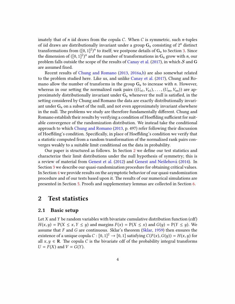
imately that of n iid draws from the copula C . When C is symmetric, such n-tuples

of iid draws are distributionally invariant under a group Gn consisting of 2n

distinct

transformations from ([0, 1]2)n to itself; we postpone details of Gn to Section 3. Since

the dimension of ([0, 1]2)n and the number of transformations in Gn grow with n, our

problem falls outside the scope of the results of Canay et al. (2017), in which S and Gare assumed �xed.

Recent results of Chung and Romano (2013, 2016a,b) are also somewhat related

to the problem studied here. Like us, and unlike Canay et al. (2017), Chung and Ro-

mano allow the number of transforms in the group Gn to increase with n. However,

whereas in our se�ing the normalized rank pairs ((Un1,Vn1), . . . , (Unn,Vnn )) are ap-

proximately distributionally invariant under Gn whenever the null is satis�ed, in the

se�ing considered by Chung and Romano the data are exactly distributionally invari-

ant under Gn on a subset of the null, and not even approximately invariant elsewhere

in the null. �e problems we study are therefore fundamentally di�erent. Chung and

Romano establish their results by verifying a condition of Hoe�ding su�cient for suit-

able convergence of the randomization distribution. We instead take the conditional

approach to which Chung and Romano (2013, p. 497) refer following their discussion

of Hoe�ding’s condition. Speci�cally, in place of Hoe�ding’s condition we verify that

a statistic computed from a random transformation of the normalized rank pairs con-

verges weakly to a suitable limit conditional on the data in probability.

Our paper is structured as follows. In Section 2 we de�ne our test statistics and

characterize their limit distributions under the null hypothesis of symmetry; this is

a review of material from Genest et al. (2012) and Genest and Neslehova (2014). In

Section 3 we describe our quasi-randomization procedure for obtaining critical values.

In Section 4 we provide results on the asymptotic behavior of our quasi-randomization

procedure and of our tests based upon it. �e results of our numerical simulations are

presented in Section 5. Proofs and supplementary lemmas are collected in Section 6.

2 Test statistics

2.1 Basic setupLetX and Y be random variables with bivariate cumulative distribution function (cdf)

H (x ,y) = P(X ≤ x ,Y ≤ y) and margins F (x ) = P(X ≤ x ) and G (y) = P(Y ≤ y). We

assume that F and G are continuous. Sklar’s theorem (Sklar, 1959) then ensures the

existence of a unique copulaC : [0, 1]2 → [0, 1] satisfyingC (F (x ),G (y)) = H (x ,y) for

all x ,y ∈ R. �e copula C is the bivariate cdf of the probability integral transforms

U = F (X ) and V = G (Y ).

4

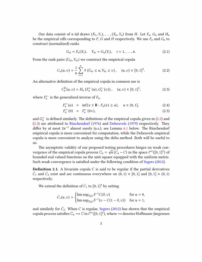
Our data consist of n iid draws (X1,Y1), . . . , (Xn,Yn ) from H . Let Fn, Gn and Hn

be the empirical cdfs corresponding to F , G and H respectively. We use Fn and Gn to

construct (normalized) ranks

Uni = Fn (Xi ), Vni = Gn (Yi ), i = 1, . . . ,n. (2.1)

From the rank pairs (Uni ,Vni ) we construct the empirical copula

Cn (u,v ) =1

n

n∑i=1

1 (Uni ≤ u,Vni ≤ v ) , (u,v ) ∈ [0, 1]2. (2.2)

An alternative de�nition of the empirical copula in common use is

CD

n (u,v ) = Hn(F←n (u),G←n (v )

), (u,v ) ∈ [0, 1]

2, (2.3)

where F←n is the generalized inverse of Fn,

F←n (u) = inf {x ∈ R : Fn (x ) ≥ u}, u ∈ (0, 1], (2.4)

F←n (0) = F←n (0+), (2.5)

and G←n is de�ned similarly. �e de�nitions of the empirical copula given in (2.2) and

(2.3) are a�ributed to Ruschendorf (1976) and Deheuvels (1979) respectively. �ey

di�er by at most 2n−1almost surely (a.s.); see Lemma 6.1 below. �e Ruschendorf

empirical copula is more convenient for computation, while the Deheuvels empirical

copula is more convenient to analyze using the delta method. Both will be useful to

us.

�e asymptotic validity of our proposed testing procedures hinges on weak con-

vergence of the empirical copula process Cn =√n (Cn −C ) in the space `∞([0, 1]

2) of

bounded real valued functions on the unit square equipped with the uniform metric.

Such weak convergence is satis�ed under the following condition of Segers (2012).

De�nition 2.1. A bivariate copula C is said to be regular if the partial derivatives

C1 and C2 exist and are continuous everywhere on (0, 1) × [0, 1] and [0, 1] × (0, 1)respectively.

We extend the de�nition of C1 to [0, 1]2

by se�ing

C1(u,v ) =

lim supδ↓0 δ−1C (δ ,v ) for u = 0,

lim supδ↓0 δ−1(v −C (1 − δ ,v )) for u = 1,

and similarly for C2. When C is regular, Segers (2012) has shown that the empirical

copula process satis�esCn C in `∞([0, 1]2), where denotes Ho�mann-Jørgensen

5

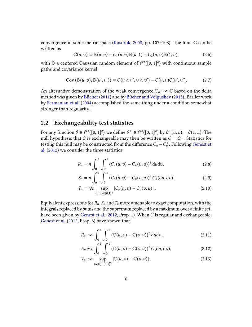
convergence in some metric space (Kosorok, 2008, pp. 107–108). �e limit C can be

wri�en as

C(u,v ) = B(u,v ) − C1(u,v )B(u, 1) − C2(u,v )B(1,v ), (2.6)

with B a centered Gaussian random element of `∞([0, 1]2) with continuous sample

paths and covariance kernel

Cov (B(u,v ),B(u′,v′)) = C (u ∧ u′,v ∧v′) −C (u,v )C (u′,v′). (2.7)

An alternative demonstration of the weak convergence Cn C based on the delta

method was given by Bucher (2011) and by Bucher and Volgushev (2013). Earlier work

by Fermanian et al. (2004) accomplished the same thing under a condition somewhat

stronger than regularity.

2.2 Exchangeability test statisticsFor any function θ ∈ `∞([0, 1]

2) we de�ne θ> ∈ `∞([0, 1]2) by θ>(u,v ) = θ (v,u). �e

null hypothesis that C is exchangeable may then be wri�en as C = C>. Statistics for

testing this null may be constructed from the di�erenceCn −C>n . Following Genest et

al. (2012) we consider the three statistics

Rn = n

∫1

0

∫1

0

(Cn (u,v ) −Cn (v,u))2

dudv, (2.8)

Sn = n

∫1

0

∫1

0

(Cn (u,v ) −Cn (v,u))2Cn (du, dv ), (2.9)

Tn =√n sup

(u,v )∈[0,1]2

|Cn (u,v ) −Cn (v,u) | . (2.10)

Equivalent expressions forRn, Sn andTn more amenable to exact computation, with the

integrals replaced by sums and the supremum replaced by a maximum over a �nite set,

have been given by Genest et al. (2012, Prop. 1). WhenC is regular and exchangeable,

Genest et al. (2012, Prop. 3) have shown that

Rn

∫1

0

∫1

0

(C(u,v ) − C(v,u))2 dudv, (2.11)

Sn

∫1

0

∫1

0

(C(u,v ) − C(v,u))2C (du, dv ), (2.12)

Tn sup

(u,v )∈[0,1]2

|C(u,v ) − C(v,u) | . (2.13)

6

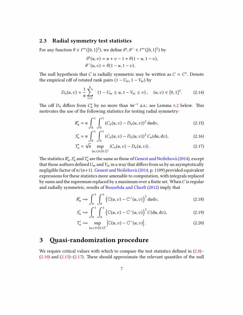
2.3 Radial symmetry test statisticsFor any function θ ∈ `∞([0, 1]

2), we de�ne θ s,θ ∈ `∞([0, 1]2) by

θ s(u,v ) = u +v − 1 + θ (1 − u, 1 −v ),

θ(u,v ) = θ (1 − u, 1 −v ).

�e null hypothesis that C is radially symmetric may be wri�en as C = Cs. Denote

the empirical cdf of rotated rank pairs (1 −Uni , 1 −Vni ) by

Dn (u,v ) =1

n

n∑i=1

1 (1 −Uni ≤ u, 1 −Vni ≤ v ) , (u,v ) ∈ [0, 1]2. (2.14)

�e cdf Dn di�ers from Cs

n by no more than 4n−1a.s.; see Lemma 6.2 below. �is

motivates the use of the following statistics for testing radial symmetry:

R′n = n

∫1

0

∫1

0

(Cn (u,v ) − Dn (u,v ))2

dudv, (2.15)

S′n = n

∫1

0

∫1

0

(Cn (u,v ) − Dn (u,v ))2Cn (du, dv ), (2.16)

T ′n =√n sup

(u,v )∈[0,1]2

|Cn (u,v ) − Dn (u,v ) | . (2.17)

�e statisticsR′n, S′n andT ′n are the same as those of Genest and Neslehova (2014), except

that those authors de�nedUni andVni in a way that di�ers from us by an asymptotically

negligible factor ofn/(n+1). Genest and Neslehova (2014, p. 1109) provided equivalent

expressions for these statistics more amenable to computation, with integrals replaced

by sums and the supremum replaced by a maximum over a �nite set. WhenC is regular

and radially symmetric, results of Bouzebda and Cher� (2012) imply that

R′n

∫1

0

∫1

0

(C(u,v ) − C(u,v )

)2

dudv, (2.18)

S′n

∫1

0

∫1

0

(C(u,v ) − C(u,v )

)2

C (du, dv ), (2.19)

T ′n sup

(u,v )∈[0,1]2

���C(u,v ) − C(u,v )��� . (2.20)

3 �asi-randomization procedureWe require critical values with which to compare the test statistics de�ned in (2.8)–

(2.10) and (2.15)–(2.17). �ese should approximate the relevant quantiles of the null

7

limit distributions given in (2.11)-(2.13) and (2.18)-(2.20). �e approach taken by Gen-

est et al. (2012) and Genest and Neslehova (2014) was to use the bootstrap procedures

of Remillard and Scaillet (2009) and Bucher and De�e (2010) to generate bootstrap

versions of the empirical copula process Cn, and thereby approximate the null limit

distribution of the relevant statistic. We will propose a di�erent resampling scheme

similar to randomization tests, narrowly tailored to the symmetry testing problem. It

delivers substantially improved small sample performance in simulations reported in

Section 5.

Suppose for a moment that F and G are known, so that we observe n iid pairs

(Ui ,Vi ) = (F (Xi ),G (Yi )) whose common bivariate cdf is the copula C . A randomiza-

tion test of a hypothesis about C may be possible if there is a �nite group G of trans-

formations from [0, 1]2

to itself such that, when the hypothesis is satis�ed, д(U ,V )D=

(U ,V ) for all д ∈ G. For testing bivariate exchangeability and radial symmetry it is

enough to consider a group of two transformations G = {π 0,π 1}. �e transformations

π 0: [0, 1]

2 → [0, 1]2

and π 1: [0, 1]

2 → [0, 1]2

are given by

π 0(u,v ) = (u,v ) and π 1(u,v ) = (v,u) (3.1)

when our hypothesis is exchangeability, and by

π 0(u,v ) = (u,v ) and π 1(u,v ) = (1 − u, 1 −v ) (3.2)

when our hypothesis is radial symmetry. It is easy to check that either choice of Gis a group under the operation of composition. Using G we can construct a second

group Gn of 2n

transformations from ([0, 1]2)n to itself by se�ing Gn = {дτ : τ =

(τ1, . . . ,τn ) ∈ {0, 1}n}, where

дτ ((u1,v1), . . . , (un,vn )) = (πτ1 (u1,v1), . . . ,πτn (un,vn )) . (3.3)

Again, it is easy to check that Gn is a group under the operation of composition. More-

over, when the relevant symmetry hypothesis is satis�ed, our sample of pairs satis�es

д ((U1,V1), . . . , (Un,Vn ))D= ((U1,V1), . . . , (Un,Vn )) for all д ∈ Gn . (3.4)

Given an arbitrary test statisticWn =Wn ((U1,V1), . . . , (Un,Vn )), property (3.4) can

be used to justify the construction of an exact level α randomization test of our sym-

metry hypothesis. �e procedure, as described by Romano (1990), is as follows.

Procedure 3.1 (Randomization test).

1. Compute Wn (дτ ((U1,V1), . . . , (Un,Vn ))) for each дτ ∈ Gn. Denote by W (1)n ≤

W (2)n ≤ · · · ≤W (2n )

n the ordered values of these statistics.

8

2. Let k = 2n − b2nαc, where b·c rounds down to the nearest integer. Determine

the number M+ ofW (·)n ’s that are strictly greater thanW (k )

n , and the number M0

that are equal toW (k )n .

3. Reject the null ifWn >W(k )n . Reject the null with probability (2nα −M+)/M0

if

Wn =W(k )n . Do not reject the null ifWn <W

(k )n .

It can be shown that, when the null hypothesis of symmetry is true, this procedure

leads us to reject it with probability exactly equal to α . See Romano (1989, 1990) and

references therein for further details on randomization tests.

Unfortunately a pure randomization test of the kind just described is not feasible

for our hypothesis testing problem because, since F and G are not known, we do not

observe pairs (Ui ,Vi ) drawn from C . In their place, we observe rank pairs (Uni ,Vni )based on preliminary estimates of the margins F and G, but these rank pairs do not

satisfy the exact group invariance property (3.4). A randomization test of symme-

try applied to our rank pairs will not achieve exact size, and cannot be expected to

achieve correct size asymptotically because relevant uncertainty about the margins is

not properly accounted for. We instead propose a modi�ed randomization procedure

which accounts for uncertainty about margins and will be shown to deliver asymp-

totically valid inference.

Let Wn = Wn ((Uni ,Vni ), . . . , (Unn,Vnn )) be the statistic of interest. Our procedure

for computing critical values forWn is as follows.

Procedure 3.2 (�asi-randomization test).

1. Select a transform дτ ∈ Gn. Set((U ∗n1,V ∗n1

), . . . , (U ∗nn,V∗nn )

)= дτ ((Un1,Vn1), . . . , (Unn,Vnn )) .

2. For i = 1, . . . ,n compute

U ∗ni =1

n

n∑j=1

1

(U ∗nj ≤ U ∗ni

), V ∗ni =

1

n

n∑j=1

1

(V ∗nj ≤ V ∗ni

).

3. ComputeW τn =Wn ((U

∗n1, V ∗n1

), . . . , (U ∗nn, V∗nn )).

4. Repeat steps 1–3 until all 2n

statistics W τn associated with the 2

nindices τ ∈

{0, 1}n have been computed. Let wn denote the k thsmallest of these statistics,

where k = 2n − b2nαc.

9

5. Reject the null ifWn > wn. Do not reject the null ifWn ≤ wn.

Procedure 3.2 di�ers in two ways from a standard randomization test of symme-

try applied to the rank pairs (Uni ,Vni ). �e essential distinction is step 2, in which

(U ∗ni ,V∗ni ) is transformed to (U ∗ni , V

∗ni ). If we were to drop step 2 and use (U ∗ni ,V

∗ni ) in

place of (U ∗ni , V∗ni ) in step 3, our method of constructing critical values would not prop-

erly account for uncertainty about the margins F and G. We will say more about this

at the end of Section 4.2. A secondary distinction between Procedures 3.1 and 3.2 is

that in the la�er we do not randomize between rejecting and not rejecting when our

test statistic is exactly equal to our critical value. �is is because the justi�cation for

our quasi-randomization test is only asymptotic, and the probability of the test statis-

tic being exactly equal to the critical value is asymptotically negligible. Procedure 3.2

therefore does not literally involve randomization.

�ough Procedure 3.2 does not involve randomization, to study its asymptotic

properties it will be useful to consider the behavior ofW τn when τ is drawn randomly

from Gn. Suppose we were to choose as τ an n-tuple of Bernoulli random variables

each taking the values zero and one with equal probabilities, independent of one an-

other and of the data. �e corresponding transform дτ would then be a random draw

from the uniform distribution over Gn, and the critical valuewn computed in step 4 of

Procedure 3.2 would be the conditional (1−α )-quantile ofW τn given the data. �at is,

wn = Qn (1 − α ), where

Qn (u) = inf

{x ∈ R : P(W τ

n ≤ x | (X1,Y1), . . . , (Xn,Yn )) ≥ u}. (3.5)

�e critical value wn computed in Procedure 3.2 can therefore be viewed as the con-

ditional (1 − α )-quantile of the randomized statisticW τn given the data. We will show

in Section 4 that, when the null of symmetry is satis�ed, the conditional law of W τn

given the data asymptotically approximates the unconditional law of the test statistic

Wn. Consequently, our critical value wn approximates the (1 − α )-quantile of the law

ofWn under the null, as desired.

In practice it may be computationally infeasible to evaluate all 2n

statistics W τn

corresponding to the 2n

transforms дτ ∈ Gn, even with modest sample sizes. In this

case, randomization may be used to obtain a feasible test. Instead of repeating steps

1–3 of Procedure 3.2 2n

times, we may repeat them some large number of times N .

Each time we select a transform дτ ∈ Gn in step 1, we should do so at random and

with replacement, choosing each possible transform with equal probabilities. �is

amounts to generating τ as an independent n-tuple of Bernoulli random variables,

each taking the values zero and one with equal probabilities. In step 4 of Procedure

3.2 we then set our critical value equal to the k thsmallest of the N computed statistics,

10

where k = N − bNαc. So long as N is large, our critical value should be close to wn,

the conditional (1 − α )-quantile ofW τn given the data.

4 Asymptotic properties

4.1 Conditional weak convergence of quasi-randomized statis-tics

�ough our quasi-randomization test is motivated by and conceptually most similar to

a randomization test, we will study it using techniques most o�en used to demonstrate

the asymptotic validity of bootstrap tests. Such demonstrations generally hinge upon

the conditional law of a bootstrapped statistic converging in a suitable sense to a target

distribution. �e conditional law we refer to here is the law obtained by holding the

data �xed and allowing the random weights used to generate the bootstrapped statistic

to vary. �e analysis of our procedure will be similar, in that it hinges upon suitable

convergence of the conditional law of the randomized statistic W τn . However in this

case the source of random variation is not a collection of bootstrap weights, but rather

a random n-tuple τ = (τ1, . . . ,τn ) that indexes transforms in the group Gn.

�roughout this section, τ represents an n-tuple of independent Bernoulli random

variables each taking the values zero and one with equal probabilities, jointly inde-

pendent of the data (X1,Y1), . . . , (Xn,Yn ). For n ∈ N, ξ τn is an element of a metric space

D depending on the data and τ , and ξn is an element of D depending on the data but

not on τ . �e following notion of convergence is from Kosorok (2008, pp. 19–20).

De�nition 4.1. If ξ is a tight random element of D then we say that ξ τn weakly con-

verges to ξ conditional on the data in probability, and write ξ τnP

τ ξ , if

1. supf ∈BL1 (D) |Eτ f (ξτn ) − Ef (ξ ) | → 0 in outer probability and

2. Eτ f (ξτn )∗ − Eτ f (ξ

τn )∗ → 0 in probability for every f ∈ BL1(D),

where BL1(D) is the set of real Lipschitz functions on D with level and Lipschitz con-

stant bounded by one, Eτ is expectation over τ holding the data �xed, and f (ξ τn )∗

and

f (ξ τn )∗ are the minimal measurable majorant and maximal measurable minorant of

f (ξ τn ) with respect to the data and random index jointly.

�e second condition in De�nition 4.1, which asserts a form of conditional asymp-

totic measurability, allows us to handle cases where ξ τn is not Borel measurable. While

this level of generality can be useful in other contexts, whenever the symbols orP

τ

11

are used in this paper, each member of the convergent sequence will in fact be Borel

measurable. �is is true even in the nonseparable space D = `∞([0, 1]2). To see why,

note that the empirical copulaCn is uniquely determined by the n2coordinate projec-

tions Cn (i/n, j/n), i, j = 1, . . . ,n, and that each of these projections can only take the

values 0,n−1, 2n−1, . . . , 1. �us Cn can take only �nitely many values in `∞([0, 1]2),

and since the projections Cn (i/n, j/n) are random variables, Cn must be a simple map

into `∞([0, 1]2). Similarly, Dn is a simple map into `∞([0, 1]

2). �e weakly convergent

or conditionally weakly convergent sequences we consider in this paper are all simple,

hence Borel measurable.

�eorems 4.3 and 4.4 below establish that the randomized statistic W τn satis�es

W τn

P

τ W , where the law ofW coincides with the weak limit ofWn when the null of

symmetry is satis�ed. From this conditional weak convergence and Lemma 10.11 of

Kosorok (2008) it follows that

P(W τn ≤ c | (X1,Y1), . . . , (Xn,Yn )) → P(W ≤ c ) (4.1)

in probability for all continuity points c of the cdf ofW . Consequently, in view of (3.5),

our quasi-randomization tests control size asymptotically and are consistent against

arbitrary violations of symmetry. �e convergence (4.1) corresponds to condition (5.3)

of Chung and Romano (2013). �eorem 5.1 in their paper shows it to be equivalent to

the weak convergence

(W τn ,W

τ ′

n ) (W ,W ′), (4.2)

where W ′and τ ′ are independent copies of W and τ respectively. Condition (4.2) is

called Hoe�ding’s condition, and plays a key role in the proofs of Chung and Romano

(2013, 2016a,b). In this paper we do not make use of Hoe�ding’s condition and instead

obtain (4.1) by directly verifying thatW τn

P

τ W .

�e proofs of our main results rely on repeated applications of conditional versions

of two fundamental results on weak convergence: the continuous mapping theorem

and the delta method. We will state these here for convenience, and also because

we require a version of the conditional delta method that is somewhat di�erent to

the usual statement. �e following statement of the conditional continuous mapping

theorem is �eorem 10.8 of Kosorok (2008). We have dropped Kosorok’s measurability

condition on τ 7→ ξ τn because τ takes only �nitely many values.

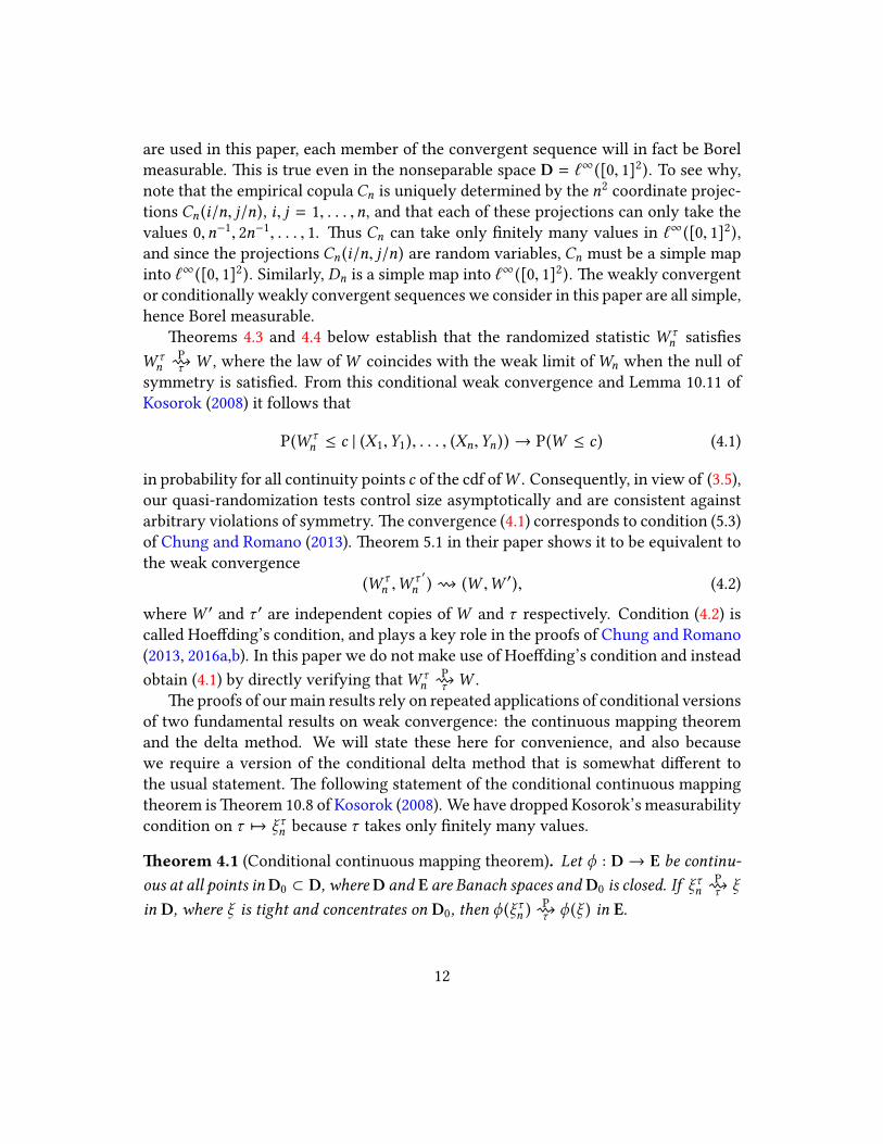
�eorem 4.1 (Conditional continuous mapping theorem). Let ϕ : D→ E be continu-ous at all points inD0 ⊂ D, where D and E are Banach spaces and D0 is closed. If ξ τn

P

τ ξ

in D, where ξ is tight and concentrates on D0, then ϕ (ξ τn )P

τ ϕ (ξ ) in E.

12

�e following statement of the conditional delta method is a version of �eorem

12.1 of Kosorok (2008), o�en referred to as the delta method for the bootstrap. It is

unusual in that we allow the weak limits X1 and X2 to di�er (and not merely by a

scalar multiple c). We have again dropped the measurability condition on τ 7→ ξ τn .

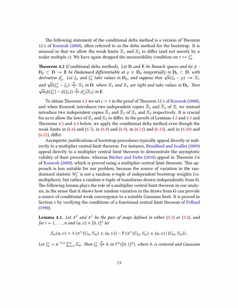
�eorem 4.2 (Conditional delta method). Let D and E be Banach spaces and let ϕ :

Dϕ ⊂ D → E be Hadamard di�erentiable at µ ∈ Dϕ tangentially to D0 ⊂ D, withderivative ϕ′µ . Let ξn and ξ τn take values in Dϕ , and suppose that

√n(ξn − µ ) X1

and√n(ξ τn − ξn )

P

τ X2 in D, where X1 and X2 are tight and take values in D0. �en√n(ϕ (ξ τn ) − ϕ (ξn ))

P

τ ϕ′µ (X2) in E.

To obtain �eorem 4.2 we set c = 1 in the proof of �eorem 12.1 of Kosorok (2008),

and when Kosorok introduces two independent copies X1 and X2 of X, we instead

introduce two independent copies X1 and X2 of X1 and X2 respectively. It is crucial

for us to allow the laws ofX1 andX2 to di�er. In the proofs of Lemmas 4.2 and 4.3 and

�eorems 4.3 and 4.4 below, we apply the conditional delta method even though the

weak limits in (6.6) and (6.7), in (6.8) and (6.9), in (6.12) and (6.13), and in (6.20) and

(6.21), di�er.

Asymptotic justi�cations of bootstrap procedures typically appeal directly or indi-

rectly to a multiplier central limit theorem. For instance, Remillard and Scaillet (2009)

appeal directly to a multiplier central limit theorem to demonstrate the asymptotic

validity of their procedure, whereas Bucher and De�e (2010) appeal to �eorem 2.6

of Kosorok (2008), which is proved using a multiplier central limit theorem. �is ap-

proach is less suitable for our problem, because the source of variation in the ran-

domized statistic W τn is not a random n-tuple of independent bootstrap weights (i.e.

multipliers), but rather a random n-tuple of transforms drawn independently from G.

�e following lemma plays the role of a multiplier central limit theorem in our analy-

sis, in the sense that it shows how random variation in the draws from G can provide

a source of conditional weak convergence to a suitable Gaussian limit. It is proved in

Section 6 by verifying the conditions of a functional central limit theorem of Pollard

(1990).

Lemma 4.1. Let π 0 and π 1 be the pair of maps de�ned in either (3.1) or (3.2), andfor i = 1, . . . ,n and (u,v ) ∈ [0, 1]

2 let

Zni (u,v ) = 1 (πτi (Uni ,Vni ) ≤ (u,v )) − P (πτi (Uni ,Vni ) ≤ (u,v ) | (Uni ,Vni )) .

Let ξ τn = n−1/2 ∑ni=1

Zni . �en ξ τnP

τ A in `∞([0, 1]2), where A is centered and Gaussian

13

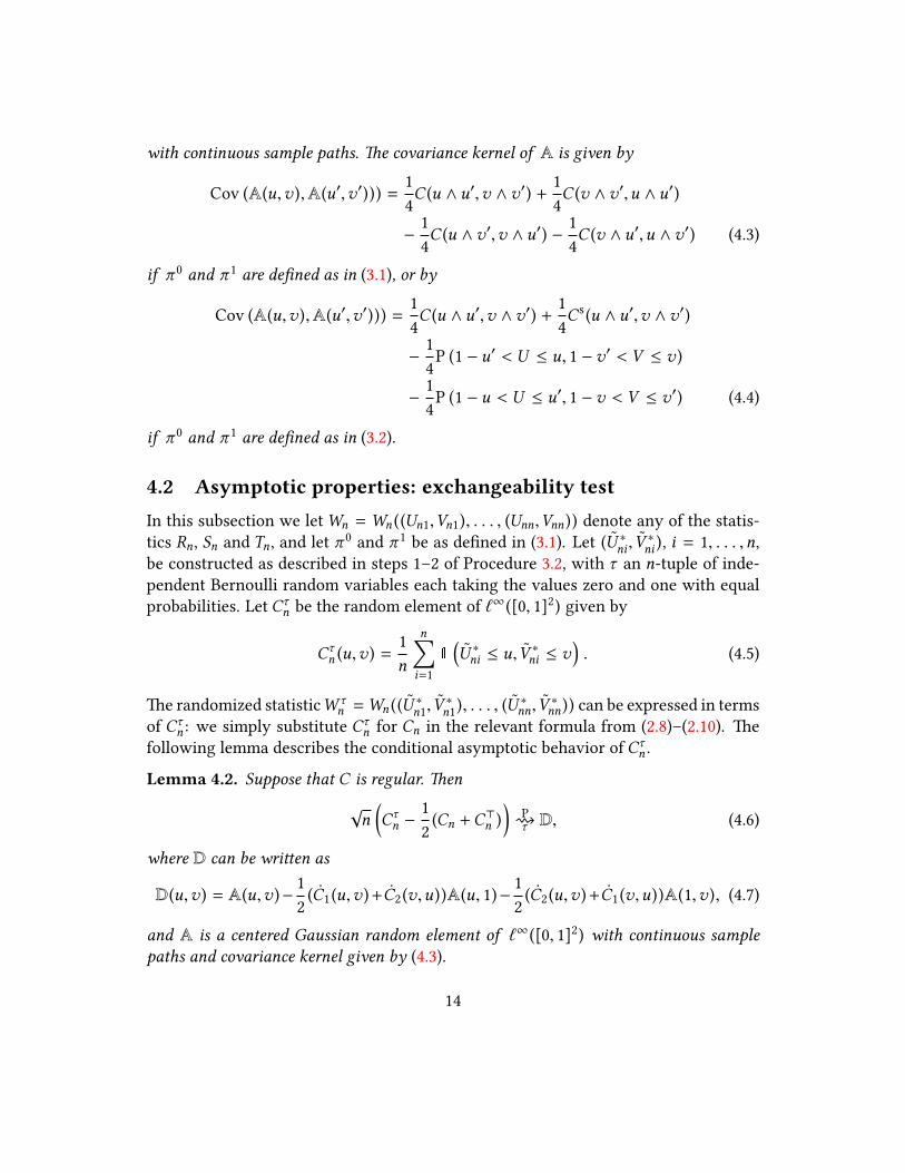
with continuous sample paths. �e covariance kernel of A is given by

Cov (A(u,v ),A(u′,v′))) =1

4

C (u ∧ u′,v ∧v′) +1

4

C (v ∧v′,u ∧ u′)

−1

4

C (u ∧v′,v ∧ u′) −1

4

C (v ∧ u′,u ∧v′) (4.3)

if π 0 and π 1 are de�ned as in (3.1), or by

Cov (A(u,v ),A(u′,v′))) =1

4

C (u ∧ u′,v ∧v′) +1

4

Cs(u ∧ u′,v ∧v′)

−1

4

P (1 − u′ < U ≤ u, 1 −v′ < V ≤ v )

−1

4

P (1 − u < U ≤ u′, 1 −v < V ≤ v′) (4.4)

if π 0 and π 1 are de�ned as in (3.2).

4.2 Asymptotic properties: exchangeability testIn this subsection we letWn =Wn ((Un1,Vn1), . . . , (Unn,Vnn )) denote any of the statis-

tics Rn, Sn and Tn, and let π 0and π 1

be as de�ned in (3.1). Let (U ∗ni , V∗ni ), i = 1, . . . ,n,

be constructed as described in steps 1–2 of Procedure 3.2, with τ an n-tuple of inde-

pendent Bernoulli random variables each taking the values zero and one with equal

probabilities. Let Cτn be the random element of `∞([0, 1]2) given by

Cτn (u,v ) =1

n

n∑i=1

1

(U ∗ni ≤ u, V ∗ni ≤ v

). (4.5)

�e randomized statisticW τn =Wn ((U

∗n1, V ∗n1

), . . . , (U ∗nn, V∗nn )) can be expressed in terms

of Cτn : we simply substitute Cτn for Cn in the relevant formula from (2.8)–(2.10). �e

following lemma describes the conditional asymptotic behavior of Cτn .

Lemma 4.2. Suppose that C is regular. �en

√n

(Cτn −

1

2

(Cn +C>n )

)P

τ D, (4.6)

where D can be wri�en as

D(u,v ) = A(u,v )−1

2

(C1(u,v )+C2(v,u))A(u, 1)−1

2

(C2(u,v )+C1(v,u))A(1,v ), (4.7)

and A is a centered Gaussian random element of `∞([0, 1]2) with continuous sample

paths and covariance kernel given by (4.3).

14

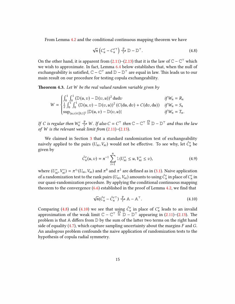
From Lemma 4.2 and the conditional continuous mapping theorem we have

√n

(Cτn −C

τ>n

)P

τ D − D>. (4.8)

On the other hand, it is apparent from (2.11)–(2.13) that it is the law of C − C> which

we wish to approximate. In fact, Lemma 6.4 below establishes that, when the null of

exchangeability is satis�ed, C − C> and D − D> are equal in law. �is leads us to our

main result on our procedure for testing copula exchangeability.

�eorem 4.3. Let W be the real valued random variable given by

W =

∫1

0

∫1

0(D(u,v ) − D(v,u))2 dudv ifWn = Rn

1

2

∫1

0

∫1

0(D(u,v ) − D(v,u))2 (C (du, dv ) +C (dv, du)) ifWn = Sn

sup(u,v )∈[0,1]2 |D(u,v ) − D(v,u) | ifWn = Tn .

If C is regular thenW τn

P

τ W . If also C = C> then C − C> D= D − D> and thus the lawof W is the relevant weak limit from (2.11)–(2.13).

We claimed in Section 3 that a standard randomization test of exchangeability

naively applied to the pairs (Uni ,Vni ) would not be e�ective. To see why, let Cτn be

given by

Cτn (u,v ) = n−1

n∑i=1

1(U ∗ni ≤ u,V ∗ni ≤ v ), (4.9)

where (U ∗ni ,V∗ni ) = π

τi (Uni ,Vni ) and π 0and π 1

are de�ned as in (3.1). Naive application

of a randomization test to the rank pairs (Uni ,Vni ) amounts to using Cτn in place ofCτn in

our quasi-randomization procedure. By applying the conditional continuous mapping

theorem to the convergence (6.6) established in the proof of Lemma 4.2, we �nd that

√n(Cτn − C

τ>n ) P

τ A − A>. (4.10)

Comparing (4.8) and (4.10) we see that using Cτn in place of Cτn leads to an invalid

approximation of the weak limit C − C>D= D − D> appearing in (2.11)–(2.13). �e

problem is that A di�ers from D by the sum of the la�er two terms on the right hand

side of equality (4.7), which capture sampling uncertainty about the margins F andG.

An analogous problem confounds the naive application of randomization tests to the

hypothesis of copula radial symmetry.

15

4.3 Asymptotic properties: radial symmetry testIn this subsection we letWn =Wn ((Un1,Vn1), . . . , (Unn,Vnn )) denote any of the statistics

R′n, S′n andT ′n, and let π 0and π 1

be as de�ned in (3.2). We letCτn be de�ned in the same

fashion as in the previous subsection, and let Dτn be the random element of `∞([0, 1]

2)given by

Dτn (u,v ) =

1

n

n∑i=1

1

(1 − U ∗ni ≤ u, 1 − V ∗ni ≤ v

).

�e randomized statisticW τn =Wn ((U

∗n1, V ∗n1

), . . . , (U ∗nn, V∗nn )) can be expressed in terms

ofCτn andDτn: we simply substituteCτn forCn andDτ

n forDn in the relevant formula from

(2.15)–(2.17). �e following lemma, analogous to Lemma 4.2, describes the conditional

asymptotic behavior of Cτn .

Lemma 4.3. Suppose that C is regular. �en√n

(Cτn −

1

2

(Cn + Dn ))

P

τ D, (4.11)

where D can be wri�en as

D(u,v ) = A(u,v ) −1

2

(C1(u,v ) + 1 − C1(1 − u, 1 −v )

)A(u, 1)

−1

2

(C2(u,v ) + 1 − C2(1 − u, 1 −v )

)A(1,v ), (4.12)

and A is a centered Gaussian random element of `∞([0, 1]2) with continuous sample

paths and covariance kernel given by (4.4).

Note that the random element D appearing in the statement of Lemma 4.3 is not

the same as the random element D appearing in the statement of Lemma 4.2. It is

apparent from (2.18)–(2.20) that the law of C−C (and alsoC , ifWn = S′n) determines

the null limit distribution ofWn. Lemma 6.5 below establishes that, when the null of

radial symmetry is satis�ed, C −C and D −D are equal in law. �is leads us to our

main result on our procedure for testing copula radial symmetry.

�eorem 4.4. Let W be the real valued random variable given by

W =

∫1

0

∫1

0

(D(u,v ) − D(u,v )

)2

dudv ifWn = R′n1

2

∫1

0

∫1

0

(D(u,v ) − D(u,v )

)2 (C (du, dv ) +Cs(du, dv )) ifWn = S′n

sup(u,v )∈[0,1]2

��D(u,v ) − D(u,v )�� ifWn = T′n .

If C is regular thenW τn

P

τ W . If also C = Cs then C − C D= D − D and thus the lawof W is the relevant weak limit from (2.18)–(2.20).

16

Copula n τα = 0.05 α = 0.1

Rn Sn Tn Rn Sn Tn

Gaussian

30

0 0.045 0.048 0.053 0.097 0.087 0.105

0.25 0.056 0.060 0.054 0.106 0.102 0.090

0.5 0.045 0.050 0.049 0.103 0.094 0.108

0.75 0.053 0.056 0.049 0.107 0.104 0.093

50

0 0.050 0.048 0.053 0.099 0.097 0.099

0.25 0.049 0.052 0.056 0.097 0.099 0.102

0.5 0.049 0.053 0.048 0.102 0.103 0.102

0.75 0.050 0.048 0.050 0.103 0.100 0.099

Clayton

30

0.25 0.042 0.050 0.042 0.086 0.104 0.087

0.5 0.046 0.054 0.053 0.111 0.106 0.118

0.75 0.045 0.046 0.048 0.104 0.096 0.100

50

0.25 0.053 0.056 0.051 0.109 0.106 0.096

0.5 0.052 0.051 0.048 0.095 0.104 0.098

0.75 0.049 0.049 0.048 0.101 0.100 0.106

Gumbel

30

0.25 0.052 0.052 0.054 0.106 0.100 0.104

0.5 0.053 0.046 0.049 0.102 0.103 0.100

0.75 0.052 0.049 0.045 0.106 0.108 0.096

50

0.25 0.056 0.046 0.049 0.100 0.100 0.101

0.5 0.051 0.050 0.054 0.107 0.108 0.103

0.75 0.051 0.055 0.053 0.100 0.101 0.101

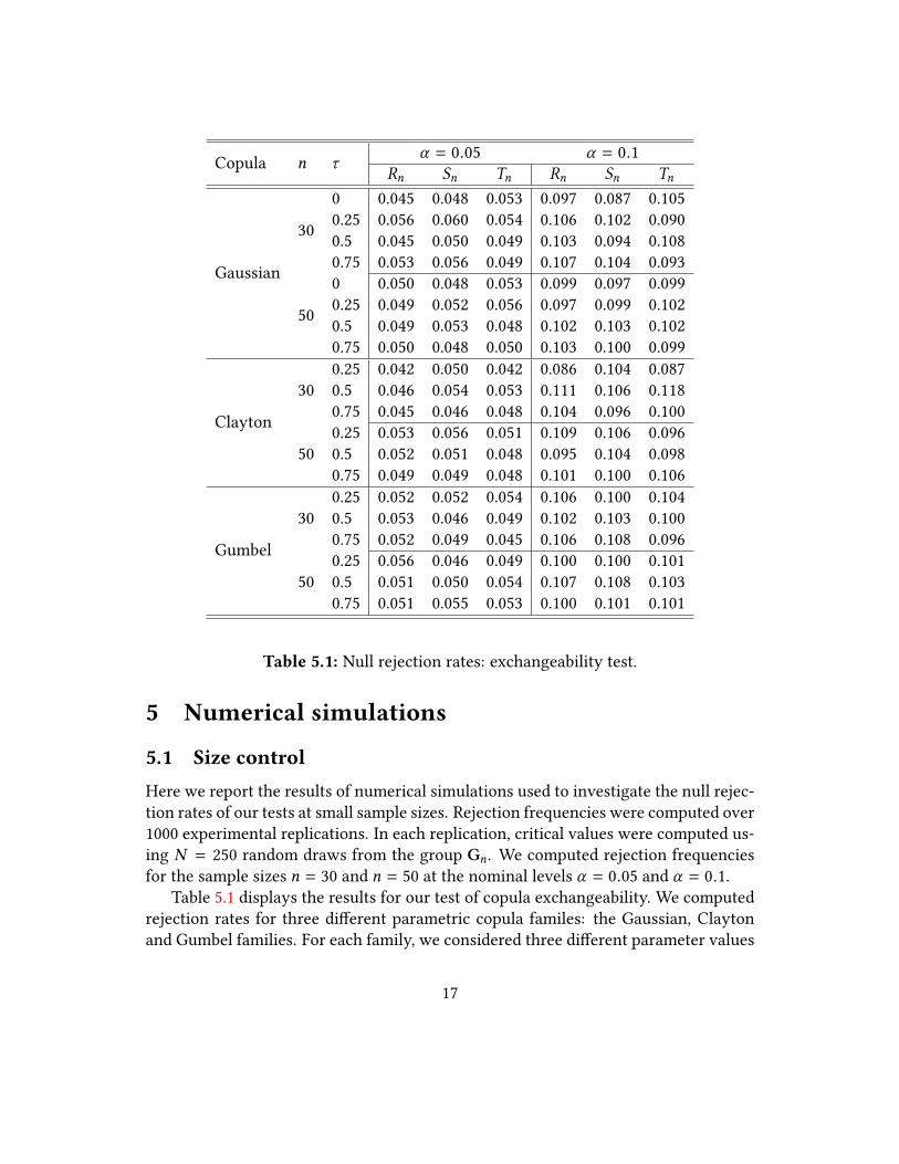
Table 5.1: Null rejection rates: exchangeability test.

5 Numerical simulations

5.1 Size controlHere we report the results of numerical simulations used to investigate the null rejec-

tion rates of our tests at small sample sizes. Rejection frequencies were computed over

1000 experimental replications. In each replication, critical values were computed us-

ing N = 250 random draws from the group Gn. We computed rejection frequencies

for the sample sizes n = 30 and n = 50 at the nominal levels α = 0.05 and α = 0.1.

Table 5.1 displays the results for our test of copula exchangeability. We computed

rejection rates for three di�erent parametric copula familes: the Gaussian, Clayton

and Gumbel families. For each family, we considered three di�erent parameter values

17

Copula n τα = 0.05 α = 0.1

R′n S′n T ′n R′n S′n T ′n

Gaussian

30

0 0.049 0.050 0.047 0.101 0.101 0.093

0.25 0.051 0.045 0.049 0.095 0.104 0.089

0.5 0.052 0.045 0.051 0.091 0.095 0.102

0.75 0.049 0.051 0.048 0.106 0.098 0.103

50

0 0.053 0.051 0.053 0.110 0.106 0.106

0.25 0.053 0.054 0.052 0.099 0.104 0.097

0.5 0.052 0.051 0.048 0.102 0.099 0.100

0.75 0.054 0.051 0.059 0.100 0.098 0.130

Frank

30

0.25 0.055 0.058 0.050 0.103 0.117 0.102

0.5 0.047 0.054 0.049 0.095 0.110 0.097

0.75 0.048 0.056 0.053 0.103 0.099 0.102

50

0.25 0.051 0.051 0.049 0.096 0.101 0.096

0.5 0.053 0.049 0.051 0.105 0.103 0.097

0.75 0.047 0.049 0.050 0.110 0.101 0.103

Cauchy

30

0.25 0.055 0.050 0.050 0.107 0.105 0.098

0.5 0.047 0.049 0.052 0.098 0.098 0.100

0.75 0.047 0.049 0.046 0.099 0.101 0.102

50

0.25 0.050 0.053 0.054 0.110 0.102 0.098

0.5 0.048 0.051 0.052 0.107 0.100 0.102

0.75 0.050 0.052 0.051 0.098 0.102 0.101

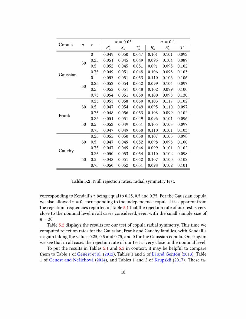
Table 5.2: Null rejection rates: radial symmetry test.

corresponding to Kendall’s τ being equal to 0.25, 0.5 and 0.75. For the Gaussian copula

we also allowed τ = 0, corresponding to the independence copula. It is apparent from

the rejection frequencies reported in Table 5.1 that the rejection rate of our test is very

close to the nominal level in all cases considered, even with the small sample size of

n = 30.

Table 5.2 displays the results for our test of copula radial symmetry. �is time we

computed rejection rates for the Gaussian, Frank and Cauchy families, with Kendall’s

τ again taking the values 0.25, 0.5 and 0.75, and 0 for the Gaussian copula. Once again

we see that in all cases the rejection rate of our test is very close to the nominal level.

To put the results in Tables 5.1 and 5.2 in context, it may be helpful to compare

them to Table 1 of Genest et al. (2012), Tables 1 and 2 of Li and Genton (2013), Table

1 of Genest and Neslehova (2014), and Tables 1 and 2 of Krupskii (2017). �ese ta-

18

bles report rejection rates for the tests of copula exchangeability and radial symmetry

proposed in those papers, using the same symmetric copulas that we have considered

here and the nominal level α = 0.05, but with sample sizes ranging between n = 100

and n = 1000. Most of these tests exhibit signi�cant size distortions at these larger

sample sizes. Generally the distortions are in the conservative direction but the ex-

changeability test of Li and Genton (2013) has rejection rates exceeding 0.15 at certain

null con�gurations, with n = 250.

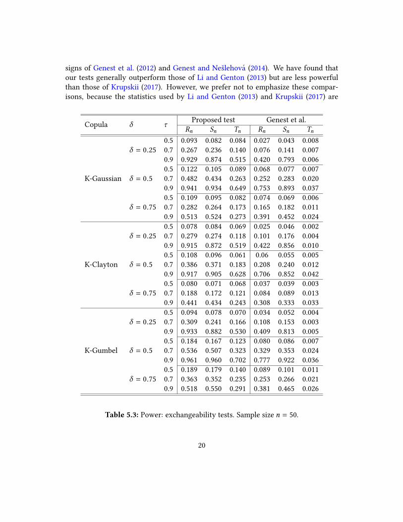
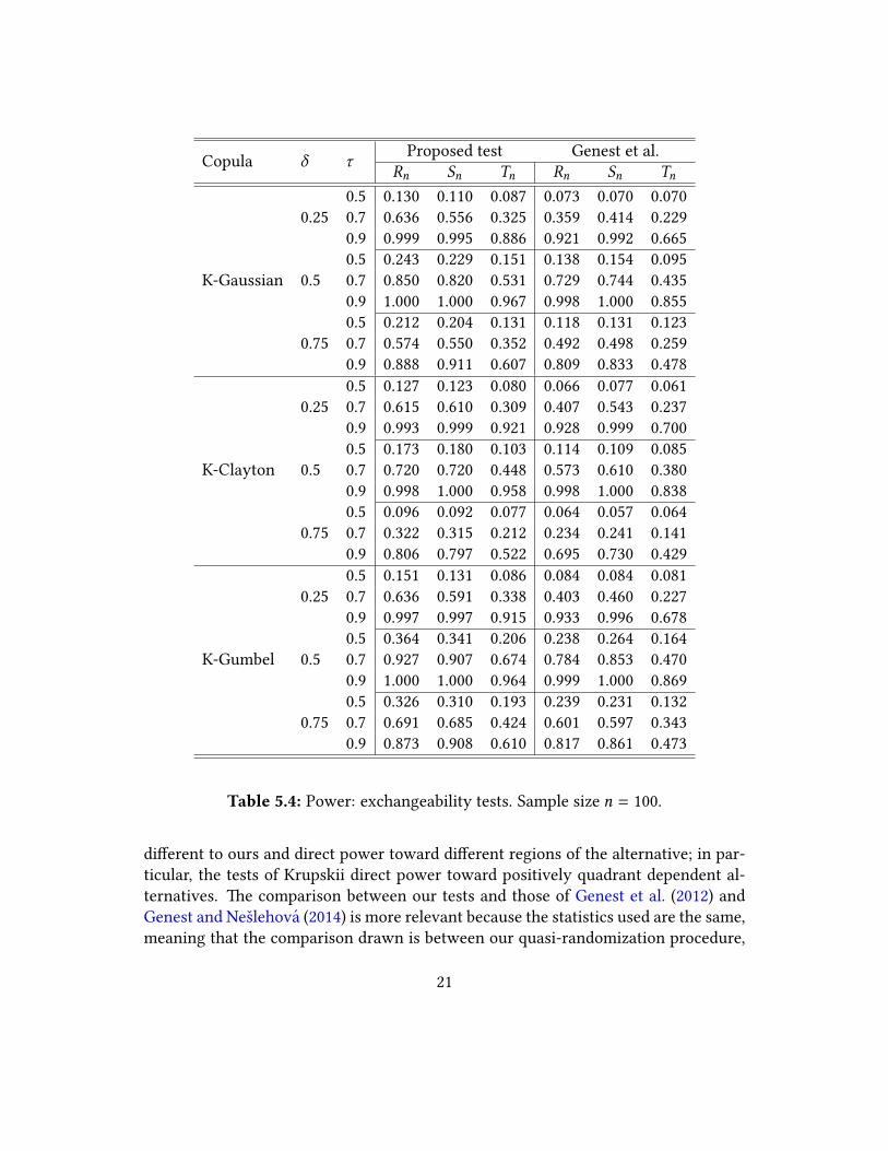
5.2 PowerIn Tables 5.3 and 5.4 we display simulated rejection frequencies for our exchangeabil-

ity tests when applied to samples drawn from various nonexchangeable copulas. As in

the previous subsection, we computed rejection frequencies over 1000 experimental

replications, and in each replication computed critical values using N = 250 random

draws from the group Gn. Our tests use a nominal level of α = 0.05. Table 5.3 reports

results obtained with n = 50, and Table 5.4 reports results obtained with n = 100.

�e nonexchangeable copulas used to produce the rejection frequencies in Tables

5.3 and 5.4 were obtained by applying the Khoudraji transform (Khoudraji, 1995) to the

Gaussian, Clayton and Gumbel copulas with parameters chosen such that Kendall’s τis equal to 0.5, 0.7 or 0.9. �e Khoudraji transform of a copulaC is given byCK

δ(u,v ) =

uδC (u1−δ ,v ), where we allow δ = 0.25, 0.5, 0.75. Genest et al. (2012) also simulate re-

jection frequencies of their exchangeability tests using these copula speci�cations; we

reproduce their numbers in Tables 5.3 and 5.4. Comparing the rejection frequencies

of our tests with those of the tests of Genest et al. (2012), we see that their bootstrap

procedure always leads to a less powerful test than our quasi-randomization proce-

dure.

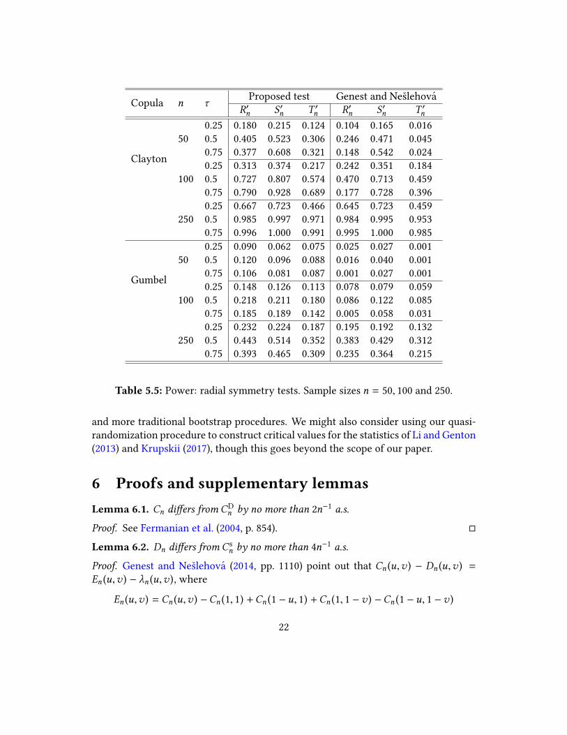
In Table 5.5 we display rejection frequencies for our radial symmetry tests when

applied to samples drawn from various radially asymmetric copulas. Rejection fre-

quencies were obtained for the Clayton and Gumbel copulas, which are radially asym-

metric, with parameters chosen such that Kendall’s τ takes the values 0.25, 0.5 and

0.75. Alongside the rejection frequencies for our tests we report corresponding rejec-

tion frequencies for the copula radial symmetry tests of Genest and Neslehova (2014),

taken directly from their paper. We �nd that our quasi-randomization procedure de-

livers substantially more power than the bootstrap procedure of Genest and Neslehova

when n = 50 and n = 100. When n = 250 our rejection frequencies are similar to those

of Genest and Neslehova.

Li and Genton (2013) and Krupskii (2017) also simulate rejection frequencies for

their tests of copula exchangeability and radial symmetry using the experimental de-

19

signs of Genest et al. (2012) and Genest and Neslehova (2014). We have found that

our tests generally outperform those of Li and Genton (2013) but are less powerful

than those of Krupskii (2017). However, we prefer not to emphasize these compar-

isons, because the statistics used by Li and Genton (2013) and Krupskii (2017) are

Copula δ τProposed test Genest et al.

Rn Sn Tn Rn Sn Tn

K-Gaussian

δ = 0.25

0.5 0.093 0.082 0.084 0.027 0.043 0.008

0.7 0.267 0.236 0.140 0.076 0.141 0.007

0.9 0.929 0.874 0.515 0.420 0.793 0.006

δ = 0.50.5 0.122 0.105 0.089 0.068 0.077 0.007

0.7 0.482 0.434 0.263 0.252 0.283 0.020

0.9 0.941 0.934 0.649 0.753 0.893 0.037

δ = 0.75

0.5 0.109 0.095 0.082 0.074 0.069 0.006

0.7 0.282 0.264 0.173 0.165 0.182 0.011

0.9 0.513 0.524 0.273 0.391 0.452 0.024

K-Clayton

δ = 0.25

0.5 0.078 0.084 0.069 0.025 0.046 0.002

0.7 0.279 0.274 0.118 0.101 0.176 0.004

0.9 0.915 0.872 0.519 0.422 0.856 0.010

δ = 0.50.5 0.108 0.096 0.061 0.06 0.055 0.005

0.7 0.386 0.371 0.183 0.208 0.240 0.012

0.9 0.917 0.905 0.628 0.706 0.852 0.042

δ = 0.75

0.5 0.080 0.071 0.068 0.037 0.039 0.003

0.7 0.188 0.172 0.121 0.084 0.089 0.013

0.9 0.441 0.434 0.243 0.308 0.333 0.033

K-Gumbel

δ = 0.25

0.5 0.094 0.078 0.070 0.034 0.052 0.004

0.7 0.309 0.241 0.166 0.108 0.153 0.003

0.9 0.933 0.882 0.530 0.409 0.813 0.005

δ = 0.50.5 0.184 0.167 0.123 0.080 0.086 0.007

0.7 0.536 0.507 0.323 0.329 0.353 0.024

0.9 0.961 0.960 0.702 0.777 0.922 0.036

δ = 0.75

0.5 0.189 0.179 0.140 0.089 0.101 0.011

0.7 0.363 0.352 0.235 0.253 0.266 0.021

0.9 0.518 0.550 0.291 0.381 0.465 0.026

Table 5.3: Power: exchangeability tests. Sample size n = 50.

20

Copula δ τProposed test Genest et al.

Rn Sn Tn Rn Sn Tn

K-Gaussian

0.25

0.5 0.130 0.110 0.087 0.073 0.070 0.070

0.7 0.636 0.556 0.325 0.359 0.414 0.229

0.9 0.999 0.995 0.886 0.921 0.992 0.665

0.5

0.5 0.243 0.229 0.151 0.138 0.154 0.095

0.7 0.850 0.820 0.531 0.729 0.744 0.435

0.9 1.000 1.000 0.967 0.998 1.000 0.855

0.75

0.5 0.212 0.204 0.131 0.118 0.131 0.123

0.7 0.574 0.550 0.352 0.492 0.498 0.259

0.9 0.888 0.911 0.607 0.809 0.833 0.478

K-Clayton

0.25

0.5 0.127 0.123 0.080 0.066 0.077 0.061

0.7 0.615 0.610 0.309 0.407 0.543 0.237

0.9 0.993 0.999 0.921 0.928 0.999 0.700

0.5

0.5 0.173 0.180 0.103 0.114 0.109 0.085

0.7 0.720 0.720 0.448 0.573 0.610 0.380

0.9 0.998 1.000 0.958 0.998 1.000 0.838

0.75

0.5 0.096 0.092 0.077 0.064 0.057 0.064

0.7 0.322 0.315 0.212 0.234 0.241 0.141

0.9 0.806 0.797 0.522 0.695 0.730 0.429

K-Gumbel

0.25

0.5 0.151 0.131 0.086 0.084 0.084 0.081

0.7 0.636 0.591 0.338 0.403 0.460 0.227

0.9 0.997 0.997 0.915 0.933 0.996 0.678

0.5

0.5 0.364 0.341 0.206 0.238 0.264 0.164

0.7 0.927 0.907 0.674 0.784 0.853 0.470

0.9 1.000 1.000 0.964 0.999 1.000 0.869

0.75

0.5 0.326 0.310 0.193 0.239 0.231 0.132

0.7 0.691 0.685 0.424 0.601 0.597 0.343

0.9 0.873 0.908 0.610 0.817 0.861 0.473

Table 5.4: Power: exchangeability tests. Sample size n = 100.

di�erent to ours and direct power toward di�erent regions of the alternative; in par-

ticular, the tests of Krupskii direct power toward positively quadrant dependent al-

ternatives. �e comparison between our tests and those of Genest et al. (2012) and

Genest and Neslehova (2014) is more relevant because the statistics used are the same,

meaning that the comparison drawn is between our quasi-randomization procedure,

21

Copula n τProposed test Genest and Neslehova

R′n S′n T ′n R′n S′n T ′n

Clayton

50

0.25 0.180 0.215 0.124 0.104 0.165 0.016

0.5 0.405 0.523 0.306 0.246 0.471 0.045

0.75 0.377 0.608 0.321 0.148 0.542 0.024

100

0.25 0.313 0.374 0.217 0.242 0.351 0.184

0.5 0.727 0.807 0.574 0.470 0.713 0.459

0.75 0.790 0.928 0.689 0.177 0.728 0.396

250

0.25 0.667 0.723 0.466 0.645 0.723 0.459

0.5 0.985 0.997 0.971 0.984 0.995 0.953

0.75 0.996 1.000 0.991 0.995 1.000 0.985

Gumbel

50

0.25 0.090 0.062 0.075 0.025 0.027 0.001

0.5 0.120 0.096 0.088 0.016 0.040 0.001

0.75 0.106 0.081 0.087 0.001 0.027 0.001

100

0.25 0.148 0.126 0.113 0.078 0.079 0.059

0.5 0.218 0.211 0.180 0.086 0.122 0.085

0.75 0.185 0.189 0.142 0.005 0.058 0.031

250

0.25 0.232 0.224 0.187 0.195 0.192 0.132

0.5 0.443 0.514 0.352 0.383 0.429 0.312

0.75 0.393 0.465 0.309 0.235 0.364 0.215

Table 5.5: Power: radial symmetry tests. Sample sizes n = 50, 100 and 250.

and more traditional bootstrap procedures. We might also consider using our quasi-

randomization procedure to construct critical values for the statistics of Li and Genton

(2013) and Krupskii (2017), though this goes beyond the scope of our paper.

6 Proofs and supplementary lemmasLemma 6.1. Cn di�ers from CD

n by no more than 2n−1 a.s.

Proof. See Fermanian et al. (2004, p. 854). �

Lemma 6.2. Dn di�ers from Cs

n by no more than 4n−1 a.s.

Proof. Genest and Neslehova (2014, pp. 1110) point out that Cn (u,v ) − Dn (u,v ) =En (u,v ) − λn (u,v ), where

En (u,v ) = Cn (u,v ) −Cn (1, 1) +Cn (1 − u, 1) +Cn (1, 1 −v ) −Cn (1 − u, 1 −v )

22

and

λn (u,v ) =1

n

n∑i=1

1(Uni = 1 − u,Vni ≥ 1 −v ) +1

n

n∑i=1

1(Uni > 1 − u,Vni = 1 −v ).

It follows that

Dn (u,v ) −Cs

n (u,v ) = λn (u,v ) −Cs

n (u,v ) +Cn (1, 1) −Cn (1 − u, 1) −Cn (1, 1 −v )

+Cn (1 − u, 1 −v ),

which simpli�es to

Dn (u,v ) −Cs

n (u,v ) = λn (u,v ) + 2 − u −v −Cn (1 − u, 1) −Cn (1, 1 −v ).

In the probability one event that there are no ties between Xi ’s or between Yi ’s, we

have |Cn (1−u, 1) − 1+u | ≤ n−1, |Cn (1, 1−v ) − 1+v | ≤ n−1

, and |λn (u,v ) | ≤ 2n−1. �

Lemma 6.3. For any u,u′,v,v′ ∈ [0, 1] we have

1

n

n∑i=1

1(u ≤ Uni ≤ u′,v ≤ Vni ≤ v′) → P(u < U ≤ u′,v < V ≤ v′) a.s.

Proof. Observe that

1(u ≤ Uni ≤ u′,v ≤ Vni ≤ v′) = 1(Uni ≤ u′,Vni ≤ v

′) − 1(Uni ≤ u,Vni ≤ v′)

− 1(Uni ≤ u′,Vni ≤ v ) + 1(Uni ≤ u,Vni ≤ v )

+ 1(Uni = u,v ≤ Vni ≤ v′) + 1(u < Uni ≤ u′,Vni = v ).

It follows that

1

n

n∑i=1

1(u ≤ Uni ≤ u′,v ≤ Vni ≤ v′) = Cn (u

′,v′) −Cn (u,v′) −Cn (u

′,v ) +Cn (u,v )

+1

n

n∑i=1

1(Uni = u,v ≤ Vni ≤ v′)

+1

n

n∑i=1

1(u < Uni ≤ u′,Vni = v ).

With probability one we cannot haveUni = u for more than one i , orVni = v for more

than one i . �erefore the last two terms on the right hand side of the last displayed

23

equality are each bounded by n−1. Pointwise strong consistency of the empirical cop-

ula thus yields the a.s. convergence

1

n

n∑i=1

1(u ≤ Uni ≤ u′,v ≤ Vni ≤ v′) → C (u′,v′) −C (u,v′) −C (u′,v ) +C (u,v )

= P(u < U ≤ u′,v < V ≤ v′).

�

Proof of Lemma 4.1. To establish conditional weak convergence we �rst note that ξ τn ,

as a map from the underlying probability space into `∞([0, 1]2), is simple and hence

Borel measurable. �e second condition in De�nition 4.1 is therefore automatically

satis�ed. To show that the �rst condition is satis�ed we will apply the functional

central limit theorem of Pollard (1990, �m. 10.6) as stated by Kosorok (2008, �m.

11.16). Adopting the notation of those authors, we let fni (u,v ) = n−1/2

1(πτi (Uni ,Vni ) ≤(u,v )), so that ξ τn =

∑ni=1

( fni−Eτ fni ). We will verify that conditions (A)–(E) of Kosorok

hold a.s.

(A) Manageability of the fni ’s with envelopes Fni = n−1/2follows from the fact

that fni (u,v ) is always monotone in (u,v ), as discussed by Kosorok (2008, p. 221).

(B) Using the fact that EτZni (u,v )Znj (u′,v′) = 0 for i , j, we obtain

Eτ ξτn (u,v )ξ

τn (u′,v′) =

1

n

n∑i=1

EτZni (u,v )Zni (u′,v′).

Further, by noting that

Zni (u,v ) =(−1)τi

2

(1(π 0(Uni ,Vni ) ≤ (u,v )) − 1(π 1(Uni ,Vni ) ≤ (u,v ))

),

we obtain

Zni (u,v )Zni (u′,v′) =

1

4

1(π 0(Uni ,Vni ) ≤ (u ∧ u′,v ∧v′))

+1

4

1(π 1(Uni ,Vni ) ≤ (u ∧ u′,v ∧v′))

−1

4

1(π 0(Uni ,Vni ) ≤ (u,v ), π 1(Uni ,Vni ) ≤ (u′,v′))

−1

4

1(π 1(Uni ,Vni ) ≤ (u,v ), π 0(Uni ,Vni ) ≤ (u′,v′)),

24

which does not depend on τi and therefore equals EτZni (u,v )Zni (u′,v′). Suppose that

π 0and π 1

are de�ned as in (3.1). �en the equalities just demonstrated imply that

Eτ ξτn (u,v )ξ

τn (u′,v′) =

1

4

Cn (u ∧ u′,v ∧v′) +

1

4

Cn (v ∧v′,u ∧ u′)

−1

4

Cn (u ∧v′,v ∧ u′) −

1

4

Cn (v ∧ u′,u ∧v′).

�e pointwise strong consistency of the empirical copula therefore implies that con-

dition (B) of Kosorok is satis�ed a.s. with

lim

n→∞Eτ ξ

τn (u,v )ξ

τn (u′,v′) =

1

4

C (u ∧ u′,v ∧v′) +1

4

C (v ∧v′,u ∧ u′)

−1

4

C (u ∧v′,v ∧ u′) −1

4

C (v ∧ u′,u ∧v′). (6.1)

Suppose instead that π 0and π 1

are de�ned as in (3.2). In this case we have

Eτ ξτn (u,v )ξ

τn (u′,v′) =

1

4

Cn (u ∧ u′,v ∧v′) +

1

4

Dn (u ∧ u′,v ∧v′)

−1

4n

n∑i=1

1(1 − u′ ≤ Uni ≤ u, 1 −v′ ≤ Vni ≤ v )

−1

4n

n∑i=1

1(1 − u ≤ Uni ≤ u′, 1 −v ≤ Vni ≤ v′),

It now follows from the pointwise strong consistency of the empirical copula and

Lemmas 6.2 and 6.3 that condition (B) of Kosorok is satis�ed a.s. with

lim

n→∞Eτ ξ

τn (u,v )ξ

τn (u′,v′) =

1

4

C (u ∧ u′,v ∧v′) +1

4

Cs(u ∧ u′,v ∧v′)

−1

4

P (1 − u′ < U ≤ u, 1 −v′ < V ≤ v )

−1

4

P (1 − u < U ≤ u′, 1 −v < V ≤ v′) . (6.2)

(C) lim supn→∞

∑ni=1

Eτ F2

ni = 1 < ∞, trivially.

(D)

∑ni=1

Eτ F2

ni1(Fni > ϵ ) = 1(n−1/2 > ϵ ) → 0 for each ϵ > 0, also trivially.

(E) �e quantity n | fni (u,v ) − fni (u′,v′) |2 is equal to one if exactly one of the in-

equalities πτi (Uni ,Vni ) ≤ (u,v ) and πτi (Uni ,Vni ) ≤ (u′,v′) is satis�ed, and is equal to

25

zero otherwise. We therefore have

n | fni (u,v ) − fni (u′,v′) |2 = 1(πτi (Uni ,Vni ) ≤ (u,v )) (1 − 1(πτi (Uni ,Vni ) ≤ (u′,v′)))

+ (1 − 1(πτi (Uni ,Vni ) ≤ (u,v )))1(πτi (Uni ,Vni ) ≤ (u′,v′))

= 1 (πτi (Uni ,Vni ) ≤ (u,v )) + 1 (πτi (Uni ,Vni ) ≤ (u′,v′))

− 2 · 1 (πτi (Uni ,Vni ) ≤ (u ∧ u′,v ∧v′)) . (6.3)

It follows that

nEτ | fni (u,v ) − fni (u′,v′) |2 =

1

2

1

(π 0(Uni ,Vni ) ≤ (u,v )

)+

1

2

1

(π 0(Uni ,Vni ) ≤ (u′,v′)

)+

1

2

1

(π 1(Uni ,Vni ) ≤ (u,v )

)+

1

2

1

(π 1(Uni ,Vni ) ≤ (u′,v′)

)− 1

(π 0(Uni ,Vni ) ≤ (u ∧ u′,v ∧v′)

)− 1

(π 1(Uni ,Vni ) ≤ (u ∧ u′,v ∧v′)

). (6.4)

De�ne

ρn ((u,v ), (u′,v′)) = *

,

n∑i=1

Eτ | fni (u,v ) − fni (u′,v′) |2+

-

1/2

.

Suppose that π 0and π 1

are de�ned as in (3.1). �en from (6.4) we have

ρn ((u,v ), (u′,v′))2 =

1

2

Cn (u,v ) +1

2

Cn (u′,v′) +

1

2

Cn (v,u) +1

2

Cn (v′,u′)

−Cn (u ∧ u′,v ∧v′) −Cn (v ∧v

′,u ∧ u′),

and so the uniform strong consistency of the empirical copula ensures that condition

(E) of Kosorok is satis�ed a.s. with

ρ ((u,v ), (u′,v′))2 =1

2

C (u,v ) +1

2

C (u′,v′) +1

2

C (v,u) +1

2

C (v′,u′)

−C (u ∧ u′,v ∧v′) −C (v ∧v′,u ∧ u′).

Suppose instead that π 0and π 1

are de�ned as in (3.2). �en from (6.4) we have

ρn ((u,v ), (u′,v′))2 =

1

2

Cn (u,v ) +1

2

Cn (u′,v′) +

1

2

Dn (u,v ) +1

2

Dn (u′,v′)

−Cn (u ∧ u′,v ∧v′) − Dn (u ∧ u

′,v ∧v′), (6.5)

and so the uniform strong consistency of the empirical copula along with Lemma 6.2

ensures that condition (E) of Kosorok is satis�ed a.s. with

ρ ((u,v ), (u′,v′))2 =1

2

C (u,v ) +1

2

C (u′,v′) +1

2

Cs(u,v ) +1

2

Cs(u′,v′)

−C (u ∧ u′,v ∧v′) −Cs(u ∧ u′,v ∧v′).

26

Having veri�ed that Kosorok’s conditions (A)–(E) hold a.s., it remains to verify

Kosorok’s almost measurable Suslin (AMS) condition. From (6.3) we have

n∑i=1

| fni (u,v ) − fni (u′,v′) |2 =

1

n

n∑i=1

1 (πτi (Uni ,Vni ) ≤ (u,v ))

+1

n

n∑i=1

1 (πτi (Uni ,Vni ) ≤ (u′,v′))

−2

n

n∑i=1

1 (πτi (Uni ,Vni ) ≤ (u ∧ u′,v ∧v′)) .

With π 0and π 1

de�ned as in either (3.1) or (3.2), πτi (Uni ,Vni ) takes values on the

grid Tn = {(i/n, j/n) : 0 ≤ i, j ≤ n}. We therefore have inf (u,v )∈Tn

∑ni=1| fni (u,v ) −

fni (u′,v′) |2 = 0 for every (u′,v′) ∈ [0, 1]

2, with the in�mum achieved by choosing

(u,v ) ∈ Tn to be the largest grid point in the rectangle [0,u′] × [0,v′]. �is proves

separability of the fni ’s, which by Lemma 11.15 of Kosorok (2008) is su�cient for the

AMS condition. We have now veri�ed that all conditions of �eorem 11.16 of Kosorok

(2008) hold a.s. Its conclusion tells us that supf ∈BL1 (`∞ ([0,1]2)) |Eτ f (ξ

τn ) − Ef (A) | → 0

a.s., where A is a centered Gaussian random element with covariance kernel given by

the expression on the right-hand side of equality (6.1) when π 0and π 1

are given by

(3.1), and by the expression on the right-hand side of equality (6.2) when π 0and π 1

are given by (3.2). Moreover, the sample paths of A are continuous with respect to the

semimetric ρ, hence also with respect to the Euclidean metric. �

Proof of Lemma 4.2. De�ne Cτn as in (4.9) and observe that

√n(Cτn −

1

2(Cn + C>n )) =

n−1/2 ∑ni=1

Zni , with the summands Zni de�ned as in Lemma 4.1. From Lemma 4.1 we

have

√n

(Cτn −

1

2

(Cn +C>n )

)P

τ A, (6.6)

where A is a centered Gaussian process with covariance kernel given by (4.3). From

the weak convergence

√n(Cn−C ) C and the continuous mapping theorem we also

have

√n

(1

2

(Cn +C>n ) −

1

2

(C +C>))

1

2

(C + C>). (6.7)

Let DΦ be the set of bivariate cdfs on [0, 1]2

with margins grounded at zero, and

let Φ : DΦ → `∞([0, 1]

2) be the map that sends a cdf H ∈ DΦ with margins H1 and

H2 to H (H←1, H←

2). �eorem 2.4 of Bucher and Volgushev (2013) establishes that Φ is

Hadamard di�erentiable at any regular copula in DΦ tangentially to

D0 = {h ∈ C : h(0,u) = h(u, 0) = h(1, 1) = 0 for all u ∈ [0, 1]} ,

27

where C is the space of continuous real valued functions on [0, 1]2. �e copula

1

2(C +

C>) ∈ DΦ inherits the property of regularity from the copula C ∈ DΦ. From Bucher

and Volgushev’s result we obtain the derivative of Φ at1

2(C +C>) in direction h ∈ D0:

Φ′1

2(C+C>)

h(u,v ) = h(u,v ) −1

2

(C1(u,v ) + C2(v,u)

)h(u, 1)

−1

2

(C2(u,v ) + C1(v,u)

)h(1,v ).

Note that A concentrates on D0, and that D = Φ′1

2(C+C>)

A. In view of (6.6) and (6.7) we

may therefore apply the conditional delta method to obtain

√n

(Φ(Cτn ) − Φ

(1

2

(Cn +C>n )

))P

τ D.

Now,Φ(Cτn ) is the Deheuvels empirical copula of the transformed rank pairsπτi (Uni ,Vni ),i = 1, . . . ,n, which di�ers from Cτn by no more than 2n−1

a.s. by Lemma 6.1. Further-

more, using the fact that1

2(Cn +C

>n ) has margins uniform on {n−1, 2n−1, . . . , 1} a.s., it

is easy to show that Φ( 1

2(Cn +C

>n )) di�ers from

1

2(Cn +C

>n ) by no more than 2n−1

a.s.

We therefore have (4.6) as claimed. �

Lemma 6.4. If C = C> then the random element D appearing in the statement ofLemma 4.2 satis�es D − D> D= C − C>.

Proof. Recalling (2.7), the covariance kernel of B − B> is given by

Cov((B − B>) (u,v ), (B − B>) (u′,v′))

= C (u ∧ u′,v ∧v′) −C (u,v )C (u′,v′) −C (u ∧v′,v ∧ u′) +C (u,v )C (v′,u′)

−C (v ∧ u′,u ∧v′) +C (v,u)C (u′,v′) +C (v ∧v′,u ∧ u′) −C (v,u)C (v′,u′).

When C = C>, this expression simpli�es to

Cov((B − B>) (u,v ), (B − B>) (u′,v′)) = 2C (u ∧ u′,v ∧v′) − 2C (u ∧v′,v ∧ u′),

and further, the covariance kernel of A given in (4.3) simpli�es to

Cov(A(u,v ),A(u′,v′)) =1

2

C (u ∧ u′,v ∧v′) −1

2

C (u ∧v′,v ∧ u′).

We therefore have AD= 1

2(B − B>) when C = C>. Observe that

Φ′C (B − B>) (u,v ) = B(u,v ) − B(v,u) − C1(u,v ) (B(u, 1) − B(1,u))

− C2(u,v ) (B(1,v ) − B(v, 1))

= C(u,v ) − C(v,u),

28

where we use C = C> to obtain the second equality. It follows that

D = Φ′CAD=

1

2

Φ′C (B − B>) =

1

2

(C − C>)

whenC = C>. But1

2(C−C>) − 1

2(C−C>)> = C−C>, and so our claim is proved. �

Proof of �eorem 4.3. WhenWn = Rn orWn = Tn we may easily deduce thatW τn

P

τ Wfrom Lemma 4.2 by applying the conditional continuous mapping theorem. When

Wn = Sn a more sophisticated argument is required, but since this argument is very

similar to the proof of Proposition 3 of Genest et al. (2012), we will be terse. From

Lemma 4.2 above and the conditional continuous mapping theorem we have

√n

(( √n(Cτn −C

τ>n )2

Cτn

)−

(0

1

2(Cn +C

>n )

))P

τ

((D − D>)2

D

)(6.8)

in the product space `∞([0, 1]2) × `∞([0, 1]

2). From the weak convergence

√n(Cn −

C ) C and continuous mapping theorem we also have

√n

((0

1

2(Cn +C

>n )

)−

(0

1

2(C +C>)

))

(0

1

2(C + C>)

). (6.9)

We may use (6.8) and (6.9) to justify an application of the conditional delta method

using the same operator as in Genest et al. (2012, p. 831), Hadamard di�erentiability

of which is given by Lemma 4.3 of Carabarin-Aguirre and Ivano� (2010). �is leads us

to conclude that

n

"(Cτn −C

τ>n )2dCτn

P

τ 1

2

"(D − D>)2d(C +C>);

that is,W τn

P

τ W . �e second part of �eorem 4.3 follows from Lemma 6.4. �

Proof of Lemma 4.3. De�ne Cτn as in (4.9) but with π 0and π 1

de�ned as in (3.2). Ob-

serve that

√n(Cτn −

1

2(Cn +Dn )) = n

−1/2 ∑ni=1

Zni , with the summands Zni de�ned as in

Lemma 4.1. From Lemma 4.1 we have

√n

(Cτn −

1

2

(Cn + Dn ))

P

τ A. (6.10)

From the weak convergence

√n(Cn −C ) C, the continuous mapping theorem, and

the fact that |Dn −Cs

n | ≤ 4n−1a.s. by Lemma 6.2, we also have

√n

(1

2

(Cn + Dn ) −1

2

(C +Cs))=

1

2

(√n(Cn −C ) +

√n(Cn −C )

)+

1

2

√n(Dn −C

s

n )

1

2

(C + C). (6.11)

29

We would like to use (6.10) and (6.11) to apply the conditional delta method using

Bucher and Volgushev’s result on the Hadamard di�erentiability of Φ, similar to what

we did at the analogous point in the proof of Lemma 4.2. However, there is a small

technical issue to resolve: the bivariate cdfs Cτn and1

2(Cn + Dn ) do not have margins

grounded at zero, and so do not lie in the domain of Φ. In fact, while Cn (1, 0) =Cn (0, 1) = 0 as desired, we haveDn (1, 0) = Dn (0, 1) = n

−1a.s., and Cτn (1, 0) and Cτn (0, 1)

are equal to either 0 or n−1a.s. Le�ing D denote the set of bivariate cdfs on [0, 1]

2, we

de�ne a sequence of maps Λn : D→ DΦ by Λn (H ) (u,v ) = 1(u ∧v ≥ n−1)H (u,v ). It is

easy to see that the four terms

���Λn (Cτn ) − C

τn

��� ,����Λn

(1

2

(Cn + Dn ))−

1

2

(Cn + Dn )���� ,

���Φ(Λn (C

τn )

)− Φ(Cτn )

��� and

����Φ(Λn

(1

2

(Cn + Dn )))− Φ

(1

2

(Cn + Dn )) ����

are all bounded a.s. by a constant multiple of n−1. We may therefore modify the con-

vergences (6.10) and (6.11) to obtain

√n

(Λn (C

τn ) − Λn

(1

2

(Cn + Dn )))

P

τ A. (6.12)

and

√n

(Λn

(1

2

(Cn + Dn ))−

1

2

(C +Cs))

1

2

(C + C). (6.13)

�eorem 2.4 of Bucher and Volgushev (2013) establishes that Φ is Hadamard di�er-

entiable at1

2(C + Cs) tangentially to D0, with derivative in direction h ∈ D0 given

by

Φ′1

2(C+Cs)

h(u,v ) = h(u,v ) −1

2

(C1(u,v ) + 1 − C1(1 − u, 1 −v )

)h(u, 1)

−1

2

(C2(u,v ) + 1 − C2(1 − u, 1 −v )

)h(1,v ).

Note that A concentrates on D0, and that D = Φ′1

2(C+Cs)

A. In view of (6.12) and (6.13)

we may therefore apply the conditional delta method to obtain

√n

(Φ

(Λn (C

τn )

)− Φ

(Λn

(1

2

(Cn + Dn ))))

P

τ D.

Consequently,

√n

(Φ(Cτn ) − Φ

(1

2

(Cn + Dn )))

P

τ D.

As in the proof of Lemma 4.2, Φ(Cτn ) di�ers from Cτn and Φ( 1

2(Cn + Dn )) di�ers from

1

2(Cn + Dn ) by no more than 2n−1

a.s. �us we have (4.11) as claimed. �

30

Lemma 6.5. Let D be the random element appearing in the statement of Lemma 4.3.If C = Cs then there exist centered Gaussian random elements E and F of `∞([0, 1]

2)that are equal in law and satisfy

C(u,v ) − C(1 − u, 1 −v ) = E(u,v ) − C1(u,v )E(u, 1) − C2(u,v )E(1,v ),

D(u,v ) − D(1 − u, 1 −v ) = F(u,v ) − C1(u,v )F(u, 1) − C2(u,v )F(1,v ).

Consequently, D − D D= C − C. �e covariance kernel of E and F is

Cov(E(u,v ),E(u′,v′)) = 2C (u ∧ u′,v ∧v′) − 2P(1 − u′ < U ≤ u, 1 −v′ < V ≤ v ).

Proof. Let Ψ : `∞([0, 1]2) → `∞([0, 1]

2) be the map

Ψ(θ ) (u,v ) = θ (u,v ) − θ (1 − u, 1 −v ) + θ (1 − u, 1) + θ (1, 1 −v ),

and de�ne E = Ψ(B) and F = Ψ(A), where A is as de�ned in the statement of Lemma

4.3. �e operator Ψ is continuous and linear, and the random elements A and B have

continuous sample paths and therefore take values in a separable subset of `∞([0, 1]2).

It follows from Proposition 3.7.2 of Bogachev (1998) thatE and F are centered Gaussian

random elements of `∞([0, 1]2). When C = Cs

we have Cj = 1 − Cj for j = 1, 2.

�erefore, from the de�nition of C given in (2.6),

C(u,v ) − C(1 − u, 1 −v ) = B(u,v ) − B(1 − u, 1 −v ) + B(1 − u, 1) + B(1, 1 −v )

− C1(u,v ) (B(u, 1) + B(1 − u, 1))

− C2(u,v ) (B(1,v ) + B(1, 1 −v ))

= E(u,v ) − C1(u,v )E(u, 1) − C2(u,v )E(1,v ).

Similarly, from the de�nition of D given in the statement of Lemma 4.3,

D(u,v ) − D(1 − u, 1 −v ) = F(u,v ) − C1(u,v )F(u, 1) − C2(u,v )F(1,v ).

It remains only to show that E and F have the claimed covariance kernel. First we

examine the covariance kernel of E. LetUi = F (Xi ) andVi = G (Yi ). Since B(u,v ) is the

weak limit ofn−1/2 ∑ni=1

(1(Ui ≤ u,Vi ≤ v )−C (u,v )), the continuous mapping theorem

implies that E(u,v ) is the weak limit of n−1/2 ∑ni=1

Ψ(1(Ui ≤ u,Vi ≤ v ) −C (u,v )). �e

terms in this la�er summation are centered and iid so, using the fact that Ψ(C ) = 1

when C = Cs, we �nd that

Cov (E(u,v ),E(u′,v′)) = E

((Ψ(1(Ui ≤ u,Vi ≤ v )) − 1) (Ψ(1(Ui ≤ u′,Vi ≤ v

′)) − 1)).

(6.14)

31

Observe that

1(Ui ≤ 1 − u,Vi ≤ 1 −v ) = 1(Ui ≤ 1 − u) + 1(Vi ≤ 1 −v ) − 1

+ 1(1 −Ui < u, 1 −Vi < v ).

It follows that

Ψ(1(Ui ≤ u,Vi ≤ v )) − 1 = 1(Ui ≤ u,Vi ≤ v ) − 1(Ui ≤ 1 − u,Vi ≤ 1 −v )

+ 1(Ui ≤ 1 − u) + 1(Vi ≤ 1 −v ) − 1

= 1(Ui ≤ u,Vi ≤ v ) − 1(1 −Ui < u, 1 −Vi < v ). (6.15)

It now follows from (6.14) that

Cov (E(u,v ),E(u′,v′)) = E

((1(Ui ≤ u,Vi ≤ v ) − 1(1 −Ui < u, 1 −Vi < v ))

× (1(Ui ≤ u′,Vi ≤ v′) − 1(1 −Ui < u′, 1 −Vi < v

′)))

= P (Ui ≤ u ∧ u′,Vi ≤ v ∧v′)

+ P (1 −Ui < u ∧ u′, 1 −Vi < v ∧v′)

− P (1 − u′ < Ui ≤ u, 1 −v′ < Vi ≤ v )

− P (1 − u < Ui ≤ u′, 1 −v < Vi ≤ v′)

= 2C (u ∧ u′,v ∧v′) − 2P (1 − u′ < Ui ≤ u, 1 −v′ < Vi ≤ v ) ,(6.16)

where to obtain the last equality we use the fact that (Ui ,Vi ) and (1 −Ui , 1 −Vi ) both

have continuous joint cdf C when C = Cs.

Next we examine the covariance kernel of F. By arguing as we did at the beginning

of the proof of Lemma 4.3, we deduce from Lemmas 4.1 and 6.2 that

√n

(Cτn −

1

2

(Cn +Cs

n ))

P

τ A.

Using the conditional continuous mapping theorem we then obtain

√n

(Ψ(Cτn ) −

1

2

Ψ(Cn +Cs

n ))

P

τ F.

It is simple to verify that Ψ(Cn +Cs

n ) (u,v ) = u +v +Cn (1 − u, 1) +Cn (1, 1 −v ). Since

Cn (1−u, 1) andCn (1, 1−v ) di�er by no more than n−1from 1−u and 1−v respectively

a.s., it follows that Ψ(Cn +Cs

n ) di�ers from 2 by no more than 2n−1a.s. �us

√n(Ψ(Cτn ) − 1) P

τ F. (6.17)

32

By applying (6.15) with πτi (Uni ,Vni ) in place of (Ui ,Vi ), we �nd that

√n(Ψ(Cτn ) − 1) =

1

√n

n∑i=1

(Ψ(1(πτi (Uni ,Vni ) ≤ (u,v )) − 1

)=

1

√n

n∑i=1

Wni (u,v ), (6.18)

where we de�ne

Wni (u,v ) = 1(πτi (Uni ,Vni ) ≤ (u,v )) − 1(πτi (Uni ,Vni ) > (1 − u, 1 −v )).

�e summands Zni appearing in the statement of Lemma 4.1 satisfy

2Zni (u,v ) = 1(πτi (Uni ,Vni ) ≤ (u,v )) − 1(πτi (Uni ,Vni ) ≥ (1 − u, 1 −v )).

Observe that |Wni (u,v ) − 2Zni (u,v ) | is bounded by 4 a.s. a�er summing over i =1, . . . ,n. �is follows from the fact that the �rst component of πτi (Uni ,Vni ) is equal

to 1 − u for at most two values of i a.s., and the second component of πτi (Uni ,Vni ) is

equal to 1 −v for at most two values of i a.s. Consequently, from (6.17) and (6.18), we

have

1

√n

n∑i=1

ZniP

τ 1

2

F.

It now follows from Lemma 4.1 that FD= 2A. When C = Cs

the covariance kernel of

A given in (4.4) simpli�es to

Cov(A(u,v ),A(u′,v′)) =1

2

C (u ∧ u′,v ∧v′) −1

2

P(1 − u′ < Ui ≤ u, 1 −v′ < Vi ≤ v ).

�e covariance kernel of F is 4 times the covariance kernel of A, and thus equal to the

covariance kernel of E given in (6.16). �us ED= F. �

Proof of �eorem 4.4. Lemma 6.2 implies that

|Cn (u,v ) + Dn (u,v ) −Cn (1 − u, 1 −v ) − Dn (1 − u, 1 −v ) − 2u − 2v + 2| ≤ 8n−1

a.s., and similarly |Dτn −C

τ s

n | ≤ 4n−1a.s. It follows easily that

�����

(Cτn −

1

2

(Cn + Dn ))−

(Cτn −

1

2

(Cn + Dn ))−

(Cτn − D

τn

) �����≤ 8n−1. (6.19)

From Lemma 4.3 and the conditional continuous mapping theorem we thus have

√n(Cτn − Dτ

n )P

τ D − D. When Wn = R′n or Wn = T ′n, another application of the

conditional continuous mapping theorem yieldsWnP

τ W . WhenWn = S′n, we instead

33

use Lemma 4.3, inequality (6.19) and the conditional continuous mapping theorem to

write

√n

(( √n(Cτn − D

τn )

2

Cτn

)−

(0

1

2(Cn + Dn )

))P

τ

((D − D)2

D

), (6.20)

and use (6.11), shown in the proof of Lemma 4.3, to write

√n

((0

1

2(Cn + Dn )

)−

(0

1

2(C +Cs)

))

(0

1

2(C + C)

). (6.21)

Using (6.20) and (6.21), we may apply the conditional delta method in the same way

as in the �rst paragraph of the proof of �eorem 4.3 to deduce that WnP

τ W . �e

second part of �eorem 4.4 then follows from Lemma 6.5. �

ReferencesAthey, S. and Haile, P. A. (2002). Identi�cation of standard auction models. Econo-

metrica, 70, 2107–2140.

Ang, A. and Chen, J. Asymmetric correlations of equity portfolios. Journal of Finan-cial Economics, 63, 443–494.

Beare, B. K. and Seo, J. (2014). Time irreversible copula-based Markov models. Econo-metric �eory, 30, 923–960.

Bogachev, V. I. (1998). Gaussian Measures. American Mathematical Society, Provi-

dence.

Bouzebda, S. and Cherfi, M. (2012). Test of symmetry based on copula function.

Journal of Statistical Planning and Inference, 142, 1262–1271.

Bucher, A. (2011). Statistical inference for copulas and extremes. Doctoral thesis,

Ruhr-Universitat Bochum.

Bucher, A. and Dette, H. (2010). A note on bootstrap approximations for the empir-

ical copula process. Statistics and Probability Le�ers, 80, 1925–1932.

Bucher, A. and Volgushev, S. (2013). Empirical and sequential copula processes un-

der serial dependence. Journal of Multivariate Analysis, 119, 61–70.

Canay, I. A., Romano, J. P. and Shaikh, A. (2017). Randomization tests under an

approximate symmetry assumption. Econometrica, 85, 1013–1030.

34

Carabarin-Aguirre, A. and Ivanoff, B. G. (2010). Estimation of a distribution under

generalized censoring. Journal of Multivariate Analysis, 101, 1501–1519.

Chen, Y. and Riordan, M. H. (2013). Pro�tability of product bundling. InternationalEconomic Review, 54, 35–57.

Chung, E. and Romano, J. P. (2013). Exact and asymptotically robust permutation

tests. Annals of Statistics, 41, 484–507.

Chung, E. and Romano, J. P. (2016a). Asymptotically valid and exact permutation

tests based on two-sample U-statistics. Journal of Statistical Planning and Inference,

168, 97–105.

Chung, E. and Romano, J. P. (2016b). Multivariate and multiple permutation tests.

Journal of Econometrics, 193, 76–91.

Dehgani, A., Dolati, A. and Ubeda-Flores, M. (2013). Measures of radial asymmetry

for bivariate random vectors. Statistical Papers, 54, 271–286.

Deheuvels, P. (1979). La fonction de dependance empirique et ses proprietes: Un test

non parametrique d’independance. Academie Royale de Belgique, Bulletin de la Classedes Sciences (5), 65, 274–292.

Fermanian, J. -D., Radulovic, D. and Wegkamp, M. (2004). Weak convergence of

empirical copula processes. Bernoulli, 10, 847–860.

Garcia, R. and Tsafack, G. (2011). Dependence structure and extreme comovements

in international equity and bond markets. Journal of Banking and Finance, 35, 1954–

1970.

Genest, C. and Neslehova, J. G. (2013). Assessing and modeling asymmetry in bi-

variate continuous data. In Jaworski, P., Durante, F. and Hardle, W. K. (eds), Copulaein Mathematical and �antitative Finance, 91–114. Springer, Berlin.

Genest, C. and Neslehova, J. G. (2014). On tests of radial symmetry for bivariate

copulas. Statistical Papers, 55, 1107–1119.

Genest, C., Neslehova, J. G. and �essy, J. -F. (2012). Tests of symmetry for bivariate

copulas. Annals of the Institute of Statistical Mathematics, 64, 811–834.

Harder, M. and Stadtmuller, U. (2017). Testing exchangeability of copulas in arbi-

trary dimension. Journal of Nonparametric Statistics, 29, 40–60.

35

Hendricks, K., Pinske, J. and Porter, R. H. (2003). Empirical implications of equilib-

rium bidding in �rst-price, symmetric, common value auctions. Review of EconomicStudies, 70, 115–145.

Hong, Y., Tu, J. and Zhou, G. (2002). Asymmetries in stock returns: statistical tests

and economic evaluation. Review of Financial Studies, 20, 1547–1581.

Khoudraji, A. (1995). Contributions a l’etude des copules et a la modelisation de valeursextremes bivariees. Ph.D. thesis, Universite Laval, �ebec City.

Kosorok, M. R. (2003). Bootstraps of sums of independent but not identically dis-

tributed stochastic processes. Journal of Multivariate Analysis, 84, 299–318.

Kosorok, M. R. (2008). Introduction to Empirical Processes and Semiparametric Infer-ence. Springer Series in Statistics, New York.

Krupskii, P. (2017). Copula-based measures of re�ection and permutation asymmetry

and statistical tests. Statistical Papers, in press.

Li, B. and Genton, M. G. (2013). Nonparametric identi�cation of copula structures.

Journal of the American Statistical Association, 108, 666–675.

Li, T., Perrigne, I. and Vuong, Q. (2000). Conditionally independent private informa-

tion in OCS wildcat auctions. Journal of Econometrics, 98, 129–161.

Menzel, K. (2016). Inference for games with many players. Review of Economic Studies,83, 306–337.

Milgrom, P. R. and Weber, R. J. (1982). A theory of auctions and competitive bidding.

Econometrica, 50, 1089–1122.

Nelsen, R. B. (1993). Some concepts of bivariate symmetry. Journal of NonparametricStatistics, 3, 95–101.

Nelsen, R. B. (2006). An Introduction to Copulas, 2nd ed. Springer, New York.

Nelsen, R. B. (2007). Extremes of nonexchangeability. Statistical Papers, 48, 329–336.

Okimoto, T. (2008). New evidence of asymmetric dependence structures in interna-

tional equity markets. Journal of Financial and �antitative Analysis, 43, 787–815.

Patton, A. J. (2004). On the out-of-sample importance of skewness and asymmetric

dependence for asset allocation. Journal of Financial Econometrics, 2, 130–168.

36

Patton, A. J. (2006). Modelling asymmetric exchange rate dependence. InternationalEconomic Review, 47, 527–556.

Pollard, D. (1990). Empirical Processes: �eory and Applications. Institute of Mathe-

matical Statistics, Hayward.

�essy, J. -F. (2016). On consistent nonparametric statistical tests of symmetry hy-

potheses. Symmetry, 8, 31.

Remillard, B. and Scaillet, O. (2009). Testing for equality between two copulas.

Journal of Multivariate Analysis, 100, 377–386.

Romano, J. P. (1989). Bootstrap and randomization tests of some nonparametric hy-

potheses. Annals of Statistics, 17, 141–159.

Romano, J. P. (1990). On the behavior of randomization tests without a group invari-

ance assumption. Journal of the American Statistical Association, 85, 686–692.

Ruschendorf, L. (1976). Asymptotic distributions of multivariate rank order statistics.

Annals of Statistics, 4, 912–923.

Segers, J. (2012). Asymptotics of empirical copula processes under non-restrictive

smoothness assumptions. Bernoulli, 18, 764–782.

Sklar, A. (1959). Fonctions de repartition a n dimensions et leurs marges. Publicationsof the Institute of Statistics of the University of Paris, 8, 229–231.

Tang, X. (2011). Bounds on revenue distributions in counterfactual auctions with re-

serve prices. RAND Journal of Economics, 42, 175–203.

37