1

Assembling and Testing a Neutron Detector

Dominik Wermus

Office of Science, Science Undergraduate Laboratory Internship (SULI)

Virginia Military Institute

Thomas Jefferson National Accelerator Facility

Newport News, Virginia

July 31, 2009

Prepared in partial fulfillment of the requirements of the Office of Science, Department of

Energy’s Science Undergraduate Laboratory Internship under the direction of Dr. Douglas W.

Higinbotham in the Hall A Division at Thomas Jefferson National Accelerator Facility.

Participant: __________________________________

Signature

Research Advisor: __________________________________

Signature

2

Assembling and Testing a Neutron Detector. DOMINIK WERMUS (Virginia Military Institute,

Lexington, VA 24450), DOUG HIGINBOTHAM (Thomas Jefferson National Accelerator

Facility, Newport News, VA, 23606).

ABSTRACT

Detecting neutrons is of high interest in experiments at Thomas Jefferson National

Accelerator Facility. Scientists use neutron detectors made of rectangular bars of scintillating

plastic with PMTs (photomultiplier tubes) attached to each end. When charged particles pass

through, scintillator plastic releases photons, which activate the light-sensitive PMTs. Neutrons

have a small but known probability of colliding with nuclei in the plastic and releasing protons,

which in turn produce light and are detected. A two-inch wall of lead in front blocks out nearly

all charged particles, making the array of scintillator bars a neutron detector. For several

upcoming experiments in Hall A, scientists wished to add twenty-four one-meter-long bars to an

existing detector. There were three stages to the project: physically assembling the bars, setting

up the data acquisition system, and testing the detector with cosmic rays (high-energy particles

from deep space). PMTs were taken from old bars, then were cleaned, tested and glued onto new

scintillator bars. A data acquisition system composed of an ADC (analog-to-digital converter)

and TDC (time-to-digital converter) was assembled, allowing for calibration and testing with

cosmic rays. The energy deposited by the passage of cosmic rays was used to set the PMT high

voltages. Once set, the known cosmic ray rate of 100 rays/m2·s was verified. These detectors

will be used for experiments such as E07-006 (Studying Short-Range Correlations via the Triple

Coincidence (e, e’pn) Reaction) for detecting neutrons released from a correlated pair of

nucleons.

3

INTRODUCTION

Thomas Jefferson National Accelerator Facility’s electron beam can reach energies of up

to 6 GeV, easily knocking out nucleons from targets. Detecting neutrons has been of high

interest in many experiments, including past and future short-range correlation experiments [1-

3]. Scientists at Jefferson Lab’s Hall A wanted to be able to detect neutrons more efficiently, so

they decided to expand the current detector, HAND (Hall A Neutron Detector) by adding two

layers of scintillating plastic bars. These bars could either be added behind the existing detector

or be given its own trigger layer and act as a separate detector.

Scintillating plastic gives off a constant glow: this is because charged particles passing

through the material cause the electrons to emit photons in the visible spectrum. The more

energetic the charged particle, the more photons are released. A particle detector can be made as

simply as gluing a light detector to a bar of scintillator and wrapping it in masking tape (blocking

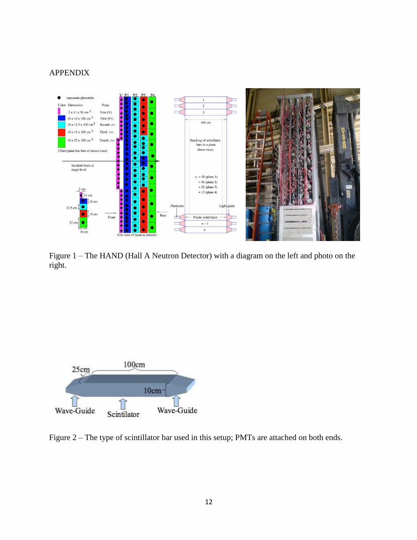
out natural light). Specifically, the HAND is made up of meter-long rectangular bars covered in

black masking tape with one photomultiplier tube (PMT) attached to each end. There are eighty-

eight bars in total, standing tall in five rows back-to-back, with a “veto” layer making the front

(Figure 1).

Since neutrons have no net charge, they are not explicitly detected by scintillators.

Instead, a neutron has a small probability of hitting a nucleus and releasing a proton, which then

releases photons in the plastic. 10 cm-thick bars will detect about 10% of the neutrons passing

through. Two bars back-to-back will detect another 10% of that (19% total), and so on.

Unwanted charged particles such as protons and electrons must be filtered out; this is done with a

thin layer of “veto” bars which have very little chance of detecting neutrons, but almost certainly

4

detect charged particles. Signals given in the veto layer are used to remove charged particle

events off-line. A two-inch lead wall in the hall can also be used to filter out charged particles

before they ever reach the detector.

A neutron detector is simply a charged-particle detector that uses electronics and

shielding to filter out unwanted particles. Neutrons release charged particles through nuclear

reactions inside the detector itself. The neutron detector was assembled with this approach. There

were three phases to the project: physically assembling the bars, hooking up the data acquisition

system (DAQ) and hardware systems, and performing the cosmic ray tests.

PHYSICAL ASSEMBLY

The bars, ordered from Kent State University, are made of 100 cm long, 10 x 25 cm

rectangular clear scintillating plastic (Figure 2). Two triangular “light guides” are fixed at each

end, narrowed to allow the round 5” diameter PMTs to be attached. The entire body of the bar is

wrapped in black masking tape to shield out natural light. Twenty-four new bars were ordered,

so forty-eight PMTs would be needed.

In Hall A’s storage shack there contained an old detecting array whose scintillator bars

had yellowed from use. These PMTs, however, were still good, and as the type used (Photonis

XP4578/B) cost around $3000 each, it was budget-wise to reuse them. A total of forty-two were

salvaged (saving $136,000), removed by cutting through the silicon glue while being careful not

to cause any shock or heavy vibrations that would break the sensitive vacuum-sealed chambers.

The PMTs were returned to the Test Lab, where the surface of each PMT was cleaned with

alcohol, removing any smudges which would block out light.

5

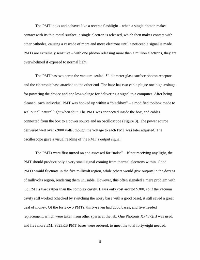
The PMT looks and behaves like a reverse flashlight – when a single photon makes

contact with its thin metal surface, a single electron is released, which then makes contact with

other cathodes, causing a cascade of more and more electrons until a noticeable signal is made.

PMTs are extremely sensitive – with one photon releasing more than a million electrons, they are

overwhelmed if exposed to normal light.

The PMT has two parts: the vacuum-sealed, 5”-diameter glass-surface photon receptor

and the electronic base attached to the other end. The base has two cable plugs: one high-voltage

for powering the device and one low-voltage for delivering a signal to a computer. After being

cleaned, each individual PMT was hooked up within a “blackbox” – a modified toolbox made to

seal out all natural light when shut. The PMT was connected inside the box, and cables

connected from the box to a power source and an oscilloscope (Figure 3). The power source

delivered well over -2000 volts, though the voltage to each PMT was later adjusted. The

oscilloscope gave a visual reading of the PMT’s output signal.

The PMTs were first turned on and assessed for “noise” – if not receiving any light, the

PMT should produce only a very small signal coming from thermal electrons within. Good

PMTs would fluctuate in the five millivolt region, while others would give outputs in the dozens

of millivolts region, rendering them unusable. However, this often signaled a mere problem with

the PMT’s base rather than the complex cavity. Bases only cost around $300, so if the vacuum

cavity still worked (checked by switching the noisy base with a good base), it still saved a great

deal of money. Of the forty-two PMTs, thirty-seven had good bases, and five needed

replacement, which were taken from other spares at the lab. One Photonis XP4572/B was used,

and five more EMI 9823KB PMT bases were ordered, to meet the total forty-eight needed.

6

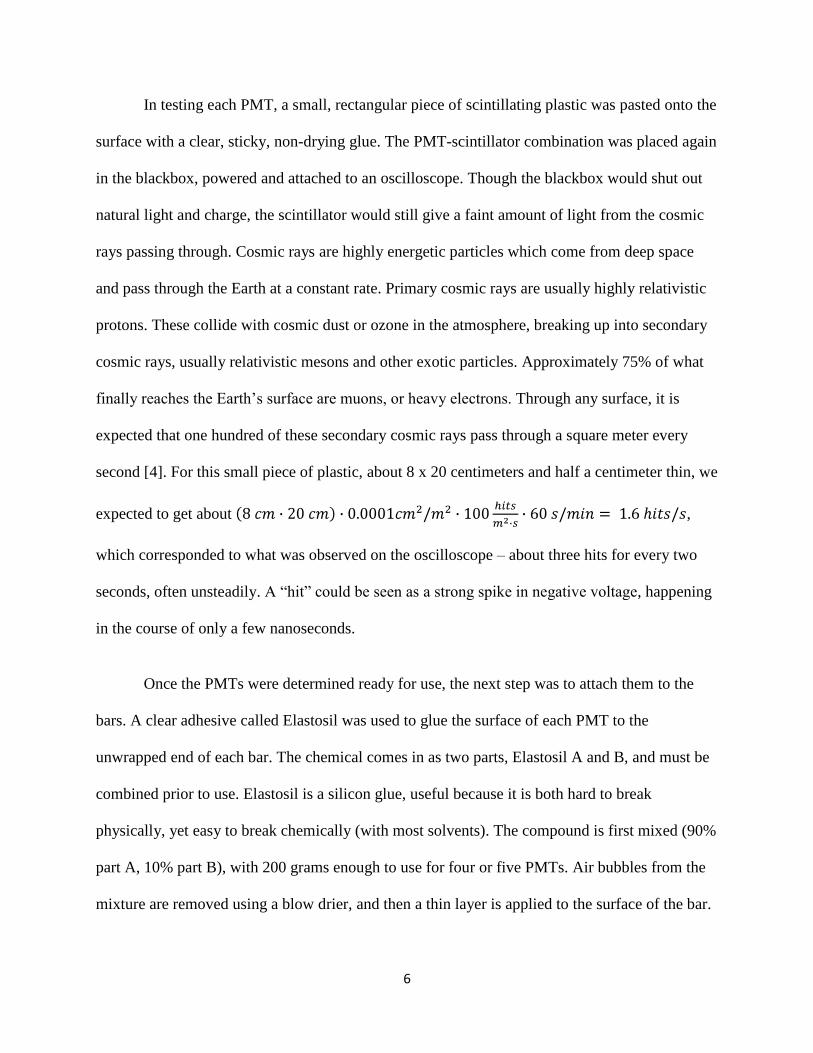
In testing each PMT, a small, rectangular piece of scintillating plastic was pasted onto the

surface with a clear, sticky, non-drying glue. The PMT-scintillator combination was placed again

in the blackbox, powered and attached to an oscilloscope. Though the blackbox would shut out

natural light and charge, the scintillator would still give a faint amount of light from the cosmic

rays passing through. Cosmic rays are highly energetic particles which come from deep space

and pass through the Earth at a constant rate. Primary cosmic rays are usually highly relativistic

protons. These collide with cosmic dust or ozone in the atmosphere, breaking up into secondary

cosmic rays, usually relativistic mesons and other exotic particles. Approximately 75% of what

finally reaches the Earth’s surface are muons, or heavy electrons. Through any surface, it is

expected that one hundred of these secondary cosmic rays pass through a square meter every

second [4]. For this small piece of plastic, about 8 x 20 centimeters and half a centimeter thin, we

expected to get about ,

which corresponded to what was observed on the oscilloscope – about three hits for every two

seconds, often unsteadily. A “hit” could be seen as a strong spike in negative voltage, happening

in the course of only a few nanoseconds.

Once the PMTs were determined ready for use, the next step was to attach them to the

bars. A clear adhesive called Elastosil was used to glue the surface of each PMT to the

unwrapped end of each bar. The chemical comes in as two parts, Elastosil A and B, and must be

combined prior to use. Elastosil is a silicon glue, useful because it is both hard to break

physically, yet easy to break chemically (with most solvents). The compound is first mixed (90%

part A, 10% part B), with 200 grams enough to use for four or five PMTs. Air bubbles from the

mixture are removed using a blow drier, and then a thin layer is applied to the surface of the bar.

7

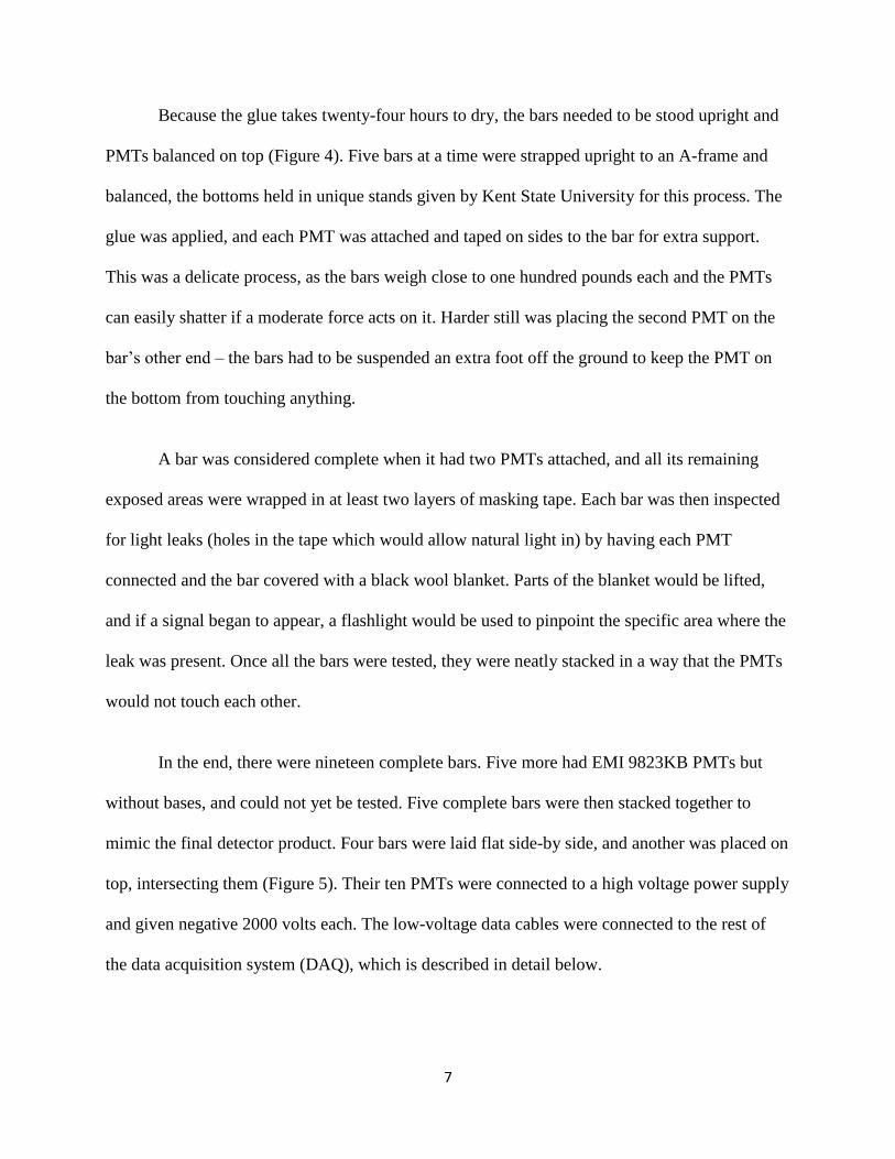
Because the glue takes twenty-four hours to dry, the bars needed to be stood upright and

PMTs balanced on top (Figure 4). Five bars at a time were strapped upright to an A-frame and

balanced, the bottoms held in unique stands given by Kent State University for this process. The

glue was applied, and each PMT was attached and taped on sides to the bar for extra support.

This was a delicate process, as the bars weigh close to one hundred pounds each and the PMTs

can easily shatter if a moderate force acts on it. Harder still was placing the second PMT on the

bar’s other end – the bars had to be suspended an extra foot off the ground to keep the PMT on

the bottom from touching anything.

A bar was considered complete when it had two PMTs attached, and all its remaining

exposed areas were wrapped in at least two layers of masking tape. Each bar was then inspected

for light leaks (holes in the tape which would allow natural light in) by having each PMT

connected and the bar covered with a black wool blanket. Parts of the blanket would be lifted,

and if a signal began to appear, a flashlight would be used to pinpoint the specific area where the

leak was present. Once all the bars were tested, they were neatly stacked in a way that the PMTs

would not touch each other.

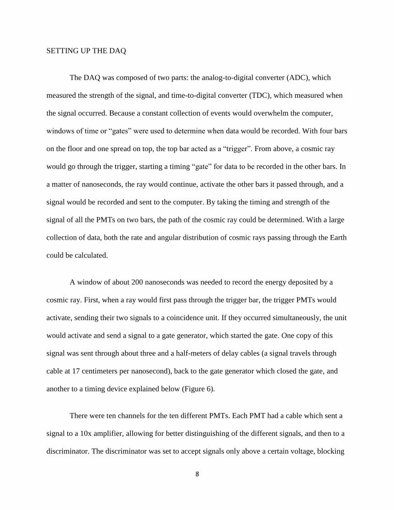
In the end, there were nineteen complete bars. Five more had EMI 9823KB PMTs but

without bases, and could not yet be tested. Five complete bars were then stacked together to

mimic the final detector product. Four bars were laid flat side-by side, and another was placed on

top, intersecting them (Figure 5). Their ten PMTs were connected to a high voltage power supply

and given negative 2000 volts each. The low-voltage data cables were connected to the rest of

the data acquisition system (DAQ), which is described in detail below.

8

SETTING UP THE DAQ

The DAQ was composed of two parts: the analog-to-digital converter (ADC), which

measured the strength of the signal, and time-to-digital converter (TDC), which measured when

the signal occurred. Because a constant collection of events would overwhelm the computer,

windows of time or “gates” were used to determine when data would be recorded. With four bars

on the floor and one spread on top, the top bar acted as a “trigger”. From above, a cosmic ray

would go through the trigger, starting a timing “gate” for data to be recorded in the other bars. In

a matter of nanoseconds, the ray would continue, activate the other bars it passed through, and a

signal would be recorded and sent to the computer. By taking the timing and strength of the

signal of all the PMTs on two bars, the path of the cosmic ray could be determined. With a large

collection of data, both the rate and angular distribution of cosmic rays passing through the Earth

could be calculated.

A window of about 200 nanoseconds was needed to record the energy deposited by a

cosmic ray. First, when a ray would first pass through the trigger bar, the trigger PMTs would

activate, sending their two signals to a coincidence unit. If they occurred simultaneously, the unit

would activate and send a signal to a gate generator, which started the gate. One copy of this

signal was sent through about three and a half-meters of delay cables (a signal travels through

cable at 17 centimeters per nanosecond), back to the gate generator which closed the gate, and

another to a timing device explained below (Figure 6).

There were ten channels for the ten different PMTs. Each PMT had a cable which sent a

signal to a 10x amplifier, allowing for better distinguishing of the different signals, and then to a

discriminator. The discriminator was set to accept signals only above a certain voltage, blocking

9

noise and low-energy particles. If accepted, two copies were made: the first signals went to the

computer as the ADCs. The second signals went to a timing device which output the TDCs. The

ADC signal was the integral of the voltage from the opening to the closing of the timing gate,

with a reference voltage subtracted to reduce the effects of noise. The TDCs were the time the

signal arrived minus the time the gate began.

The computer was able to collect cosmic ray readings with CODA software and process

them using ROOT. CODA (Common DAQ) is a software system developed at Jefferson Lab for

the collection of data to be used in conjunction with ROOT. ROOT was developed at CERN by

physicists working with high-energy experiments where the number of events in one run can be

in the millions, and with hundreds of runs in one experiment. ROOT is useful for its processing

power and graphing capabilities [5].

TESTING WITH COSMIC RAYS

With the setup complete, data was nearly ready to be recorded. However, because each

PMT’s base is slightly unique, each PMT would need a slightly different “gain”, or amount of

power to give the same reading for the same energy particle. Quick runs were taken to check the

ADCs coming from each PMT. If the energies detected were too high, the power going to the

PMT would be lowered, and vice-versa. The gains on the PMTs were adjusted so they would all

give readings in the same range (Table 1).

Charged particles lose energy in the plastic at 2 MeV/cm. With most of the cosmic rays

coming from the atmosphere above, there would be a mean energy deposit of 50 MeV per

cosmic ray, corresponding to about 200 mV in a signal. To evaluate the rate of events detected,

10

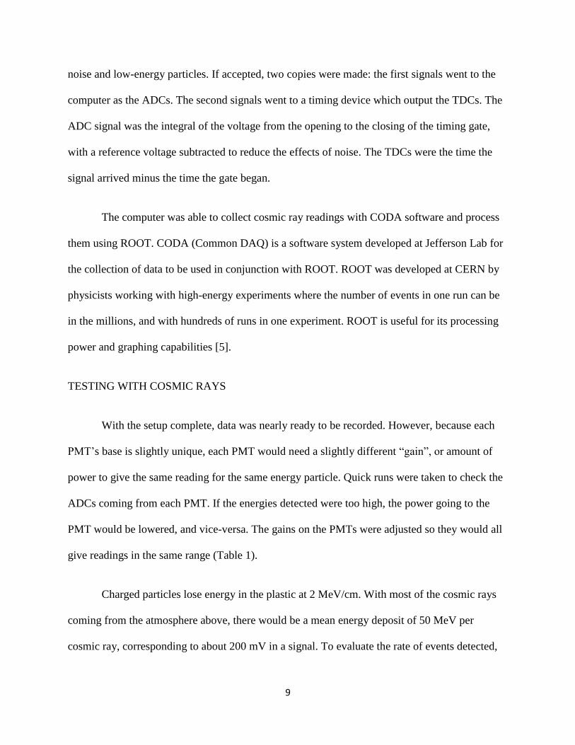
the discriminator was tested on a range of settings (Figure 7). The rate of events should have

been , reduced to 20 hits/s since not all events would be

detected by the PMTs. This corresponded to a setting of 150 mV.

The final phase of testing would be to measure the paths of the cosmic rays. A new

arrangement was set up: five bars were arranged so that one trigger bar laid flat on top of two

stacks of two bars. Large recordings were taken (two to three million events), and an evaluation

program written in ROOT displayed ADC and TDC data from each PMT in histograms (Figure

8). The difference in TDCs on a single bar could give the point of entry of the cosmic ray (Figure

9). By comparing two bars, the complete path (including angle) of a cosmic ray could be

determined. Total spatial and angular distribution of cosmic rays was calculated by adding all of

these events (Figure 10).

By examining the TDC data, there seemed to be a strong bias towards one side on each of

the bars. The reason for this is still undetermined – either there is some source giving off strong

radiation (which in the Test Lab is very possible), or the gains on the PMTs are imbalanced.

Either way, based on these results, the bars were determined ready for use. The detector will be

used for experiments such as E07-006 (Studying Short Range Correlations via the Triple

Coincidence (e, e’pn) Reaction), where an electron beam scatters paired nucleons from a target.

For the future, the bars still need to be arrayed in a metal rack just as with the original detector.

Further, a “veto” layer may still be assembled if this detector is to be used independently from

the original. A 2-inch lead wall will absorb almost all charged particles, but a thin layer of

scintillator poorly absorbs neutrons and can signal “false hits” for unwanted particles.

11

ACKNOWLEDGEMENTS

I cannot fit my feelings of gratitude in this poor little section. My summer internship was

granted by the Department of Energy SULI (Science Undergraduate Laboratory Internship)

Program. I would like to thank my mentor Doug for his great dedication, sense of humor and his

many hours of leading me to thrive in this sink-or-swim environment. For our collaboration on

this effort I would like to acknowledge physicists Eli Piasetski, Moshe Kochavi and PhD student

Or Chen from the University of Tel Aviv, who have given me the first understanding for the life

of a scientist. Next are Lisa Surles-Law and Jan Tyler for bringing the interns together and for

laughing when I did things that other scientists did not approve of. Finally, I’d like to thank

Anthony Gillespie, Gary Dezern, Ed Folts, Elena Long and everyone else who has mentored me

this summer. I am now confident I am capable of becoming a good scientist and will be happy

with my life doing so.

REFERENCES

[1] R. Subedi et al., Science 320, 1476 (2008); (10.1126/science.1156675).

[2] D. W. Higinbotham, E. Piasetzky and M. Strikman, Protons and Neutrons Cozy Up In

Nuclei and Neutron Stars, 49N1 (2009) 22-24.

[3] S. Gilad, D. Higinbotham, S. Watson, E. Piasetski, V. Sulkosky et al., Studying Short-

Range Correlations in Nuclei at the Repulsive Core Limit via the Triple Coincidence (e,e'pN)

Reaction, [JLab E07-006] (2009).

[4] C. Amsler et al. [Particle Data Group], Physics Letters B 667, 1 (2008).

[5] A. Brun and F. Rademakers, Nuclear Instrumentation Methods,. A389, 81 (1997).

12

APPENDIX

Figure 1 – The HAND (Hall A Neutron Detector) with a diagram on the left and photo on the

right.

Figure 2 – The type of scintillator bar used in this setup; PMTs are attached on both ends.

13

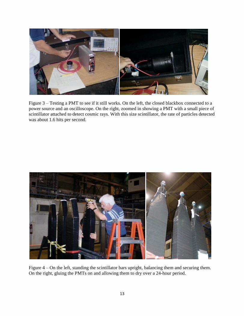
Figure 3 – Testing a PMT to see if it still works. On the left, the closed blackbox connected to a

power source and an oscilloscope. On the right, zoomed in showing a PMT with a small piece of

scintillator attached to detect cosmic rays. With this size scintillator, the rate of particles detected

was about 1.6 hits per second.

Figure 4 – On the left, standing the scintillator bars upright, balancing them and securing them.

On the right, gluing the PMTs on and allowing them to dry over a 24-hour period.

14

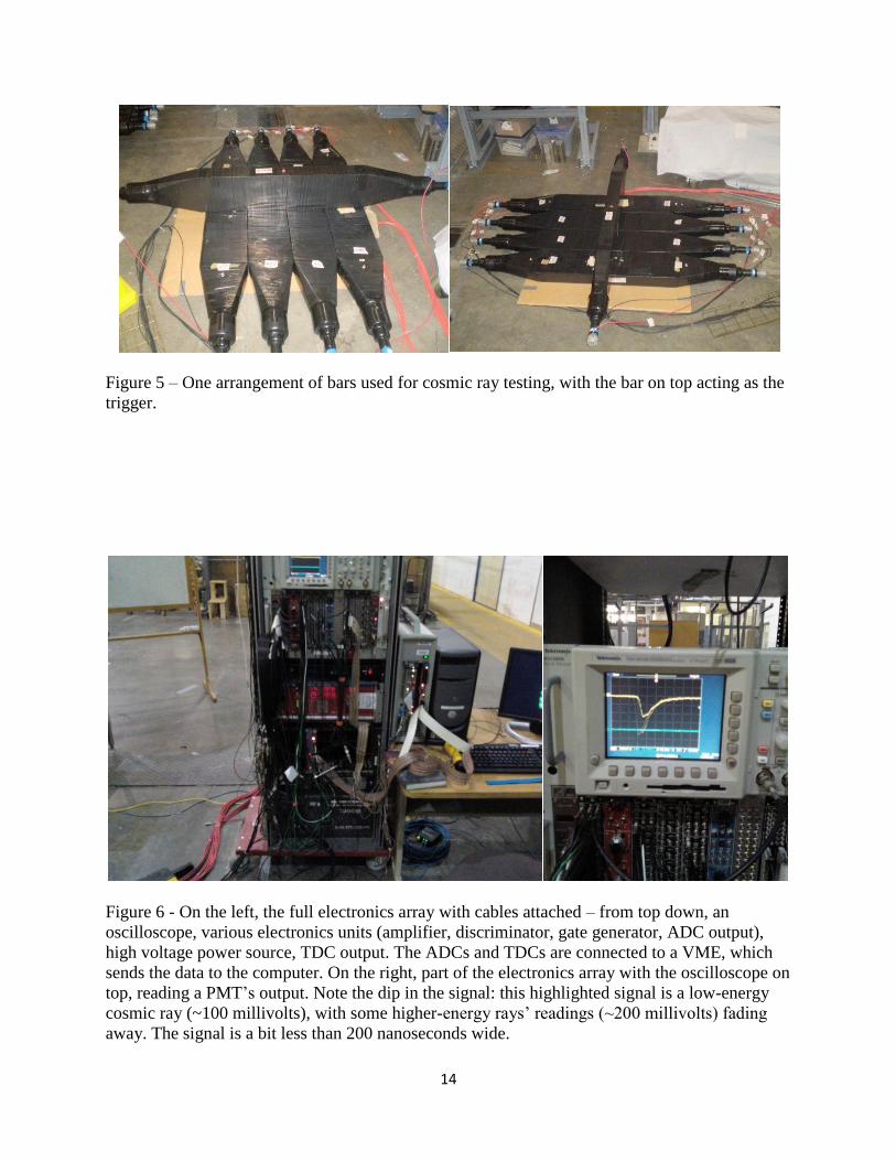
Figure 5 – One arrangement of bars used for cosmic ray testing, with the bar on top acting as the

trigger.

Figure 6 - On the left, the full electronics array with cables attached – from top down, an

oscilloscope, various electronics units (amplifier, discriminator, gate generator, ADC output),

high voltage power source, TDC output. The ADCs and TDCs are connected to a VME, which

sends the data to the computer. On the right, part of the electronics array with the oscilloscope on

top, reading a PMT’s output. Note the dip in the signal: this highlighted signal is a low-energy

cosmic ray (~100 millivolts), with some higher-energy rays’ readings (~200 millivolts) fading

away. The signal is a bit less than 200 nanoseconds wide.

15

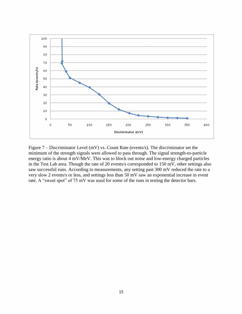
Figure 7 – Discriminator Level (mV) vs. Count Rate (events/s). The discriminator set the

minimum of the strength signals were allowed to pass through. The signal strength-to-particle

energy ratio is about 4 mV/MeV. This was to block out noise and low-energy charged particles

in the Test Lab area. Though the rate of 20 events/s corresponded to 150 mV, other settings also

saw successful runs. According to measurements, any setting past 300 mV reduced the rate to a

very slow 2 events/s or less, and settings less than 50 mV saw an exponential increase in event

rate. A “sweet spot” of 75 mV was used for some of the runs in testing the detector bars.

16

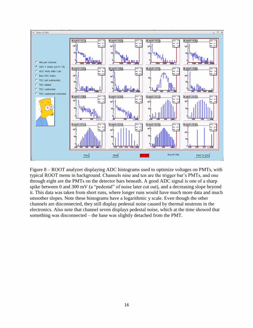
Figure 8 – ROOT analyzer displaying ADC histograms used to optimize voltages on PMTs, with

typical ROOT menu in background. Channels nine and ten are the trigger bar’s PMTs, and one

through eight are the PMTs on the detector bars beneath. A good ADC signal is one of a sharp

spike between 0 and 300 mV (a “pedestal” of noise later cut out), and a decreasing slope beyond

it. This data was taken from short runs, where longer runs would have much more data and much

smoother slopes. Note these histograms have a logarithmic y scale. Even though the other

channels are disconnected, they still display pedestal noise caused by thermal neutrons in the

electronics. Also note that channel seven displays pedestal noise, which at the time showed that

something was disconnected – the base was slightly detached from the PMT.

17

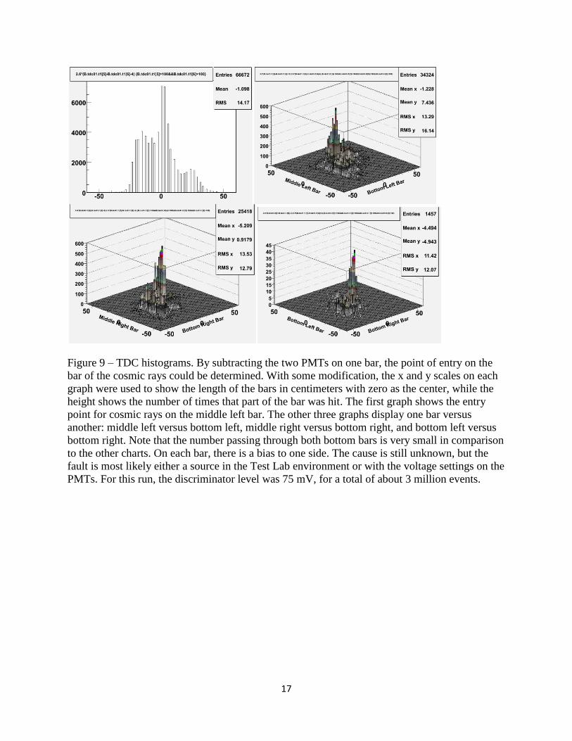
Figure 9 – TDC histograms. By subtracting the two PMTs on one bar, the point of entry on the

bar of the cosmic rays could be determined. With some modification, the x and y scales on each

graph were used to show the length of the bars in centimeters with zero as the center, while the

height shows the number of times that part of the bar was hit. The first graph shows the entry

point for cosmic rays on the middle left bar. The other three graphs display one bar versus

another: middle left versus bottom left, middle right versus bottom right, and bottom left versus

bottom right. Note that the number passing through both bottom bars is very small in comparison

to the other charts. On each bar, there is a bias to one side. The cause is still unknown, but the

fault is most likely either a source in the Test Lab environment or with the voltage settings on the

PMTs. For this run, the discriminator level was 75 mV, for a total of about 3 million events.

18

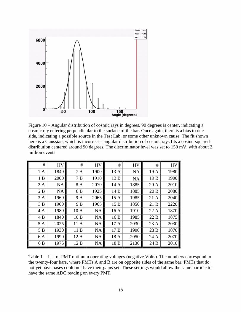
Figure 10 – Angular distribution of cosmic rays in degrees. 90 degrees is center, indicating a

cosmic ray entering perpendicular to the surface of the bar. Once again, there is a bias to one

side, indicating a possible source in the Test Lab, or some other unknown cause. The fit shown

here is a Gaussian, which is incorrect – angular distribution of cosmic rays fits a cosine-squared

distribution centered around 90 degrees. The discriminator level was set to 150 mV, with about 2

million events.

1 A 1840 7 A 1900 13 A NA 19 A 1980

1 B 2000 7 B 1910 13 B NA 19 B 1900

2 A NA 8 A 2070 14 A 1885 20 A 2010

2 B NA 8 B 1925 14 B 1885 20 B 2080

3 A 1960 9 A 2065 15 A 1985 21 A 2040

3 B 1900 9 B 1965 15 B 1850 21 B 2220

4 A 1980 10 A NA 16 A 1910 22 A 1870

4 B 1840 10 B NA 16 B 1985 22 B 1875

5 A 2025 11 A NA 17 A 2030 23 A 2030

5 B 1930 11 B NA 17 B 1900 23 B 1870

6 A 1990 12 A NA 18 A 2050 24 A 2070

6 B 1975 12 B NA 18 B 2130 24 B 2010

Table 1 – List of PMT optimum operating voltages (negative Volts). The numbers correspond to

the twenty-four bars, where PMTs A and B are on opposite sides of the same bar. PMTs that do

not yet have bases could not have their gains set. These settings would allow the same particle to

have the same ADC reading on every PMT.