Embed Size (px)
Citation preview
1
Assessing Redistribution within Social Insurance Systems.
The cases of Argentina, Brazil, Chile, Mexico and Uruguay1
Alvaro Forteza2
Departamento de Economía, Facultad de Ciencias Sociales,
Universidad de la República, Uruguay
May 18, 2011
Abstract
This paper summarizes the main findings in a series of coordinated studies conducted to assess
the impact of social security programs on the distribution of lifetime labor income in
Argentina, Brazil, Chile, Mexico and Uruguay. The country-case studies find varying degrees of
redistribution, with PAYG-DB and mixed programs redistributing more than individual savings
accounts programs. Notwithstanding, it is the Chilean individual savings accounts program,
combined with the recently reformed solidarity pillar, the one that contributes more to
reducing inequality in this group of countries.
Keywords: Redistribution, Social Security.
1 This document summarizes the findings in five country-case studies conducted simultaneously using
similar methodologies. The background papers are Fajnzylber (2011), Forteza and Mussio (2011),
Moncarz (2011) and Zylberstajn (2011). The project was financed by the World Bank. We are grateful to
David Robalino for proposing the initial idea and for his continuous support. The usual disclaimer
applies.
2
1 Introduction
The present paper summarizes the main findings of five country-case studies conducted to
analyze the impact of unemployment insurance and pension programs on the distribution of
lifetime income in Latin America (Fajnzylber 2011, Forteza and Mussio 2011, Moncarz 2011
and Zylberstajn 2011). Based on longitudinal data, we estimate econometric models of
contributions to social security and labor income and run Monte Carlo simulations of expected
life time labor income and net transfers to social security. Using these estimations we then
compute indicators of distribution and redistribution of income. We find that some programs
perform much redistribution, but the programs that redistribute more are not necessarily the
ones that make the greater contribution to reducing inequality.
The pension programs covered in our project range from the fully PAYG-DB Argentinean and
Brazilian to the individual accounts DC Chilean and Mexican programs, and also include the
Uruguayan mixed program. Unemployment insurance is based on savings accounts and
common pool schemes in Brazil and Chile and on common pool PAYG financing in Argentina
and Uruguay. Hence, our sample allows for a comparison of the redistributive impact of
different social security designs.
Previous studies show that densities of contribution are low and very heterogeneous in
Argentina, Chile and Uruguay (Forteza et al 2009). We do not have similar longitudinal studies
for Brazil and Mexico, but social security coverage of the labor force in these two countries
suggests that contribution densities cannot be much higher in Brazil and Mexico than in the
other three countries. Therefore, we are assessing social security redistribution in the
presence of low density and highly fragmented histories of contributions, considering five
social security programs with substantial differences.
In the next section we briefly describe the programs to be analyzed. In section three we
present the conceptual framework and discuss antecedents in the literature. We describe the
data and methods in sections 4 and 5. Section 6 contains the results and section 7 concludes
with some final remarks.
2 The old-age pension and unemployment insurance programs
3
In 1981, Chile pioneered a series of pension programs reforms that introduced mandatory
individual savings accounts, phasing out the traditional PAYG-DB scheme. In the nineties,
Mexico reformed its pension program along the same lines as Chile. Also in the mid nineties,
Argentina and Uruguay introduced mandatory individual savings accounts, but without
completely phasing out the PAYG-DB pillar. The result was a two pillar (or two tiers) mixed
program. Brazil did a series of parametric reforms without introducing savings accounts in its
pension program.
New reforms took place in the 2000s. The most radical of the new wave of reforms was the
Argentinean abolition of the individual savings accounts. The current scheme is a partially
funded DB program. Funds accumulated in the individual accounts were allocated to a
collective pension fund. In 2008, Chile strengthened the redistributive component of its
pension system, replacing the minimum pension and old-age assistance programs with a basic
solidarity pension and a pension supplement. Also in 2008, Uruguay adjusted its program,
loosening pension eligibility conditions.
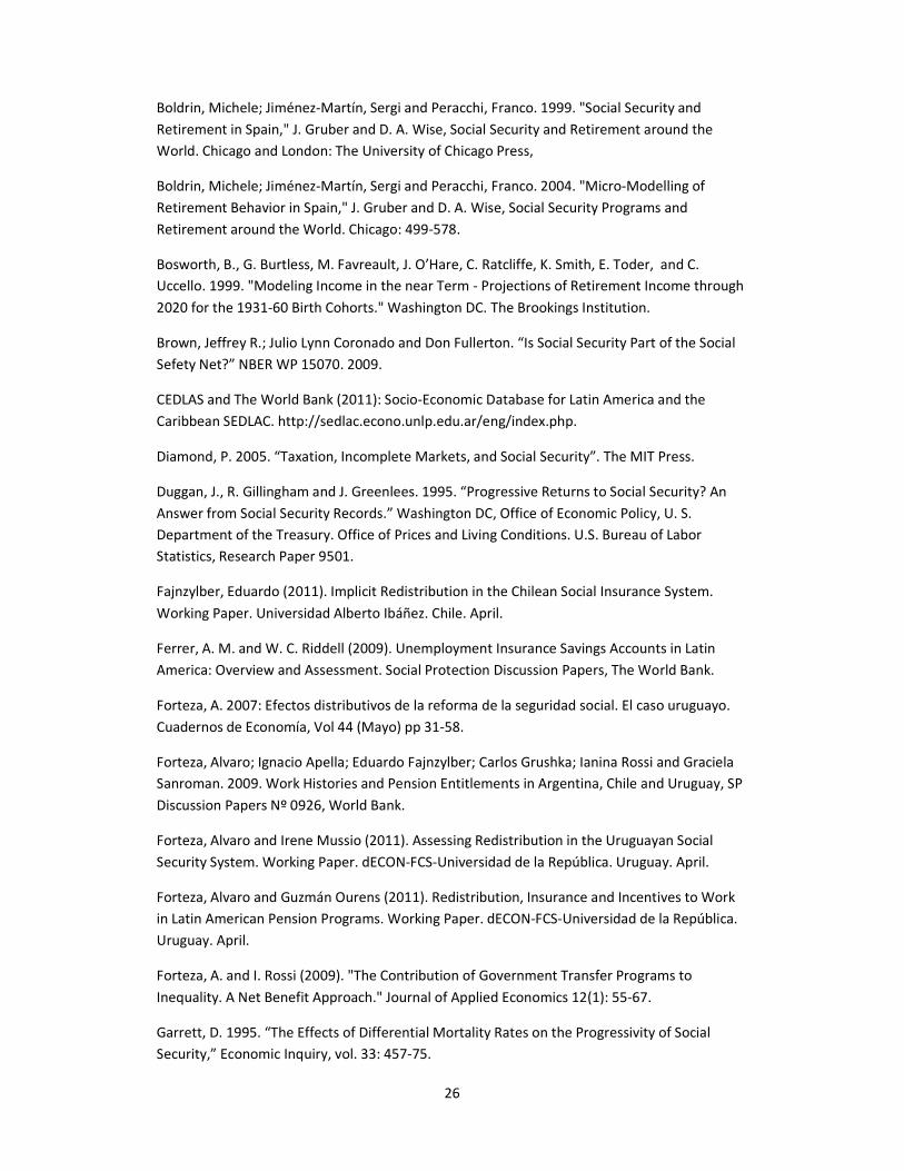
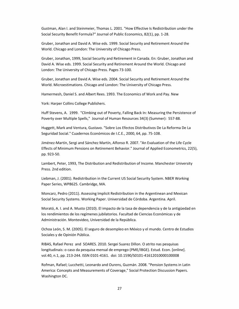
We summarize in Table 1 the main parameters of these pension programs as they are today.
These are the parameters used for the simulations in this study.
In addition, there is considerable variation in the design and scope of unemployment insurance
programs in the set of countries included in this study. Argentina and Uruguay have traditional
common pool PAYG programs, Brazil has parallel common pool and individual accounts
programs, Chile has an integrated program that combines individual accounts with social
insurance and Mexico does not have an explicit unemployment insurance program (Velásquez
2010).
The Argentinean program was enacted in 1992. It is financed out of employer contributions of
1.5% of wages on a PAYG common-pool basis and benefits are earnings related.3 The first
Brazilian unemployment program was founded in 1967 and consists of a compulsory
contribution that employers have to deposit in an individual account, called FGTS (Fundo de
Garantia do Tempo de Servico). A second program was enacted in 1986, incorporated in the
Constitution in 1988 and implemented and expanded during the nineties. This program has
common pool financing and earnings-related benefits (Barreto de Oliveira and Beltrão 2002).
3 There is also a small unemployment insurance savings accounts program in Argentina for construction
workers.
4
Chile introduced a new unemployment insurance scheme in 2002. This program combines self
and social insurance: workers and employers contribute to individual savings accounts and the
government and employers contribute to a common pool called the “solidarity fund”. Mexico
does not have an unemployment insurance program, save for the advanced age
unemployment insurance scheme (seguro de cesantía en edad avanzada) that covers
individuals aged 60 and above (Ochoa 2005). With antecedents dating to the early twentieth
century, the current Uruguayan unemployment insurance program was enacted in 1981 and
expanded in 2001 (Amarante and Bucheli 2008). It is a traditional common pool earnings
related program.
3 Conceptual framework
We assess redistribution within social insurance programs computing lifetime contributions
and benefits. Our focus is on mostly contributory programs, but some non-contributory
components cannot and should not be separated from the contributory ones. The Chilean
solidarity supplement is an example of a well integrated non contributory component in a
mostly contributory program. The financing that governments often provide in PAYG programs
is also a “non contributory” component of social security. In some cases, this financing is
incorporated in the design of the programs (for example, some points of the value added tax
are earmarked for social security in Uruguay), but in most cases governments just pay what is
needed to keep social security programs working.
Social Security programs are usually designed to redistribute income from the better to the
worse off. Most benefit formulas include explicit redistributive components, such as minimum
pensions and supplements to small pensions. Even individual accounts DC programs, which are
based on the principle of actuarial neutrality, tend to incorporate non-actuarial redistributive
ingredients.
But social security programs also redistribute income through less explicit mechanisms. First,
high mortality rates may reduce the returns low income workers get for their contributions in
pension programs when unified mortality tables are used (Garrett, 1995; Duggan et al. 1995;
Beach and Davis 1998; Brown et al. 2009).4
4 There is however contradicting evidence on the impact of differential mortality rates on social security
progressiveness. Brown et al. (2009), for example, report very small effects on the measured
5
Second, government transfers that contribute to finance social security in many countries
favor the population that is covered by the programs, which in developing countries tends to
be the better off (Rofman et al. 2008). But also these same groups are the ones that pay more
taxes, so the net effect is not clear (Forteza and Rossi, 2009). Ideally, we should trace the origin
of the funds governments spend financing social security and include those taxes in the
individuals’ cash flows.
Third, low densities of contribution may leave many workers ineligible for benefits. Low
income workers have been shown to have particularly low densities of contribution (Forteza et
al. 2009; Berstein et al. 2006). In this research project, we focused on this last channel, i.e. the
redistribution stemming from the fact that low income workers tend to have systematically
shorter contribution histories. We will not assess the impact of different mortality rates and
different coverage on implicit redistribution.
Social Security redistribution is often assessed on an annual basis, analyzing taxes paid and
benefits received by different groups of contributors. This type of analysis tends to show large
transfers among groups which depend mostly on the ratio of beneficiaries to earners within
each group. But most individuals transit from earning income and paying contributions to
receiving pension benefits along their lifecycle. Therefore, redistribution performed through
social security can be better assessed adopting a lifetime perspective (Liebman, 2001).
We run micro-simulations of lifetime income and social security contributions and benefits to
assess redistribution, focusing on intra-generational redistribution: one cohort that lives with
the current pension rules. It is worth noticing though that social security performs inter- as
well as intra-generational redistribution and there is considerable evidence that inter-
generational redistribution has been substantial, with early generations usually benefiting with
high returns to contributions (Liebman 2001, Morató and Musto, 2010).
The indicator used in this study to quantify transfers is the social security wealth, which is the
net present value of the expected lifetime flows of contributions and benefits (Gruber and
Wise, 1999, 2004; Coile and Gruber, 2001; Liebman, 2001, Brown et al. 2009). Also, we assess
the progressivity of the system by comparing the distribution of the expected pre- and post-
social security lifetime income. Pre-social security lifetime income is the present value of
progressivity of the US Social Security program of incorporating differential mortality rates by race and
education.
6
income before contributions to social security and without benefits from social security. Post-
social security income is the present value of lifetime income net of contributions to social
security and including benefits from social security. The comparison is performed based on
standard Lorenz and concentration curves, Gini indexes and an index of net redistributive
effect.
We consider the individual as the unit of analysis, but it should be noticed that redistribution in
the social security system may look very different at the family level. Gustman and Steinmeier
(2001) show that, when analyzed at the individual level, the U.S. social security looks very
redistributive, favoring low income workers, but it looks much less so at the family level (see
also Lambert 1993, p 14). In the words of Brown et al. (2009): “…much of the apparent
redistribution from Social Security occurs within, rather than between, households.”
Ideally, the assessment of the redistributive impact of social security programs should be
based on the comparison of income distribution with and without social security.5 This is not
the same as comparing pre- and post-social security income (i.e. income minus contributions
plus benefits), because social security is likely to induce changes in work hours, savings, wages
and interest rates. In this line, Huggett and Ventura (2000) simulate a fully fledged OLG model
of Social Security calibrated with US data. Forteza (2007) follows a similar approach to study
the redistributive impact of a social security reform in Uruguay. In a similar vein, albeit not to
study redistribution, Jiménez and Sánchez (2007) estimate a structural life cycle model to
assess the incentives to retire in the Spanish Social Security System. Auerbach and Kotlikoff
(1987) represents a key antecedent in this line of inquiry. One possible drawback of these
models is the assumption of full rationality, something that has been subject to much
controversy, especially regarding long run decisions like those involved in social security. After
all, the most appealed rationale for pension programs is individuals' myopia (Diamond, 2005,
chap. 4). In principle, a model with hyperbolic preferences could do the job, but solving and
calibrating these models is even more difficult than the already demanding standard
optimization, full rationality models.
5 This is the equivalent to what Lambert (1993, p 266) suggests for the assessment of the impact of
income taxes: “…the impact of an income tax can now be judged by comparing the “with-tax” income
distribution with the distribution that would pertain in the tax’s absence –the “no-tax” distribution
rather than the “pre-tax” distribution.” It is interesting to notice though, that ten of the eleven chapters
of his classical book on distribution and redistribution of income are based on the assumption of
invariant pre-tax income distribution.
7
In turn, much of fiscal incidence analysis is done on the non-behavioral type of assumption. It
is usually performed under the assumption that pre-tax income is not affected by the tax
system. Because of this, it is often interpreted as an analysis of the impact effect of the fiscal
system (Lambert, 1993, pp 153, 162, chap 11). One such example is Euromod. Sutherland
(2001) warns: “EUROMOD is better-suited to analysing some types of policy and policy change
than others. Since it is a static model, designed to calculate the immediate, “morning after”
effect of policy changes, it neither incorporates the effects of behavioural changes (i.e.
behaviour does not change) nor the long-term effect of change. Thus it is not the appropriate
tool for examining policy that is only designed to change behaviour, nor for policy that can only
have its impact in the long term (e.g. some forms of pensions policy). It is best-suited to the
analysis of policies that have an immediate effect and which depend only on current income
and circumstance.” For our analysis, we will be using life cycle models that are better suited to
assess the redistributive impact of social security policies than the typical static short run
models used in most microsimulations. However, following standard practice in
microsimulations, we will not model behavioral responses. Our approach is closer to the
literature pioneered by Gruber and Wise (1999, 2004), who designed and computed a series of
indicators of social security incentives to retire assuming no explicit behavioral responses. Our
study is also close to Liebman (2001) and Brown et al. (2009) who simulate lifetime income
and compute redistribution in US Social Security using non-behavioral models.
In our view, these two approaches are largely complementary. The optimization models have
the obvious advantage of incorporating behavioral responses, so not only the direct effects of
policies are considered, but also the indirect effects that go through behavioral changes.
However, in order to keep things manageable, these theoretically ambitious models need to
make highly stylized assumptions regarding not only individual preferences and constraints,
but also social security programs. Given our goals, this is a serious drawback. We want to
assess the lifetime implicit transfers in social security given the observed histories of
contribution in Latin American countries. We are only beginning to characterize the very
heterogeneous highly fragmented histories of contribution present in the region (Forteza et al.
2009) and quite far from having optimization models that can fit these patterns. Whether
these histories of contribution are optimal responses to social security rules and various shocks
is something we cannot answer yet. But given social security rules, it is pretty clear that these
patterns of contribution seriously condition effective net transfers to social security. Non-
behavioral micro-simulations are based on exogenously given work histories and geared to
providing insights on the social security transfers that emerge from those histories. Thanks to
8
their relative simplicity, non-behavioral models allow for a much more detailed specification of
the policy rules and work histories than intertemporal optimization models. An additional
advantage of micro-simulations is that the effects are straightforward, so no black-box issues
arise. At the very least, we can expect to capture the first-order impact effects of social
security on income distribution. The micro-simulation modeling can thus be seen as a first step
in a more ambitious research program that incorporates behavioral responses at a more
advanced phase.6
4 Data We use two sources of data: administrative records from Social Security (Uruguay and Chile)
and surveys (Argentina, Brazil, and Mexico). In what follows, we provide brief descriptions of
the databases.
4.1 Argentinean data
We used a household survey (the Encuesta Permanente de Hogares or EPH) for the period
1995-2003. 7
The EPH is carried out twice a year (May and October) covering only urban areas
(around 61% of the country total population, and 70% of the country urban population). Each
household included in the EPH, and all the individuals within it, is surveyed four consecutive
times, with a replacement rate of 25% of the sample each survey. The EPH provides detailed
information on the labor status, personal characteristics (age, gender, education, etc.) on each
individual, as well as on characteristics of the household (number of members, living
conditions, etc.).
4.2 Brazilian data
The Pesquisa Mensal de Emprego (PME), or Monthly Employment Survey, is a monthly rotating
panel of dwellers in six major metropolitan areas in Brazil (São Paulo, Rio de Janeiro, Belo
Horizonte, Salvador, Porto Alegre and Recife), compiled by IBGE. These six metropolitan areas
cover approximately 25% of the country's population. The PME survey was redesigned in
March, 2002. Currently, microdata is available since then until August, 2010.
6 An example of this strategy is the retirement research line followed by Jiménez and collaborators in
the case of Spain (Boldrin et al. 1999, 2004; Jiménez and Sánchez, 2007).
7 From the second half of 2003 the EPH suffered from an important methodological change that impede
us to extend the period of analysis, also because of the timing households are surveyed under the new
EPH this is less suitable for the purposes of the present study.
9
The survey investigates schooling, labor force, demographic, and earnings characteristics of
each resident aged 10 or more that lives on the interviewed households. This results in
approximately 100,000 individuals from 35,000 households every month. One important
feature is that there is no information on earnings not arising from labor.
The rotating scheme is as follows. Households are interviewed once per month during four
consecutive months after which they stay out of the survey for an eight-month window. After
this period, the household is interviewed again in four consecutive months. Once this last spell
is finished, the household is permanently excluded from the sample. Households are divided
into 4 rotating groups, in order to make sure that in two consecutive months 75% of the
sample is the same.
The PME does not identify individuals directly, only their households. Thus, a matching process
needs to take place. We match individuals within households over time using date of birth and
gender, but a caveat of doing this is that there might be some attrition. In fact, according to
Ribas and Soares (2010), on average 4% of the households sampled in the PME do not answer
to the survey in the following month. In order to avoid (or at least minimize) a selection bias,
the authors propose an algorithm and the inclusion of an ‘answering probability estimator’ in
an estimation à la Heckman.
In order to build the database, we match individuals (using the algorithm proposed above) that
were surveyed for two consecutive months and consider this matching as one observation.
Characteristics such as income, gender, age, marital status and schooling are taken from the
first interview (identified by t), together with labor status. The subsequent interview
(identified by t+1) gives only the new labor status and income.
4.3 Chilean data
We have access to the Base de Historias Previsionales de Afiliados Activos, Pensionados y
Fallecidos (Affiliates Pension Histories database, HPA), populated with individual contribution
records from 1981 to 2009, for a sample of participants in the pension system.8 The HPA
includes the complete contribution history (in the pension system) for a sample of
8 The sample was originally drawn as the basis for the Social Protection Survey, a panel instrument that
was taken in 2002, 2004 and 2006 for a large fraction of the individuals in the sample. The Social
Protection Survey was inspired by the American Health and Retirement Survey. For more information on
the Chilean version, see www.proteccionsocial.cl.
10
approximately 24,000 individuals, representative of the stock of affiliates of the system in July
2002.9 In addition, the dataset also includes information on the recognition bonds held by the
sampled individuals.
4.4 Mexican data
The data source is a household survey carried out by the Instituto Nacional de Estadística y
Geografía de Mexico, more specifically we use the Encuesta Nacional de Empleo (ENE). The
ENE is a continuous quarterly national survey representative of the whole population. The unit
of analysis of the ENE is the household, but with a specific questionnaire for each individual
living in it, which allows to control for personal characteristics. The replacement rate in the
sample is 20% so each unit is surveyed during five consecutive quarters after which they are
dropped from the survey. The period we work with runs form the third quarter of 2000 until
the last quarter of 2004.10
4.5 Uruguayan data
We used a random sample of the work history records of the main social security institution of
Uruguay (BPS), collected in December 2004 by the Labor History Unit of the BPS (ATYR-BPS).
Workers in the sample contributed at least one month between April 1996 and December
2004. The sample has close to 70,000 individuals.
The records are organized in five databases. One file gives personal information on individuals:
date of birth, sex and country of birth. Another file reports about the job of each person,
particularly the date of initiation of activity and the explicit end of the link between the worker
and the firm. A third file reports monthly information about the contributions. In particular, we
have information on wages and some characteristics of the job. A separate database contains
information about benefits, including the date of retirement.
This database provides detailed information about monthly contributions to social security,
gender, age, and sector of activity. Unfortunately, we do not have yet for Uruguay a survey of
socio-economic characteristics of contributors to social security. Hence, we lack some
important socio-economic characteristics like education and characteristics of the families.
9 Upon initial contribution, the individual is considered an “affiliate”.
10 A new nationwide survey, the Encuesta Nacional de Empleo y Ocupación (ENOE) started in the first
quarter of 2005. However, because of the information we require to carry out the analysis we work with
the ENE.
11
5 Methods The methodology is comprised of four steps. (i) Estimation and simulation of labor status and
labor income models. (ii) Computation of social security contributions and pensions. (iii)
Computation of pre- and post-social security lifetime income. (iv) Computation of income
distribution measures.
5.1 Labor income and labor status models
We separately estimate models for labor income and working-contributing status. We model
labor income to simulate strings of lifetime labor income, conditional on being
working/contributing. We also model labor status, i.e. whether the individual is contributing or
not, and simulate lifetime contributing status. Multiplying the simulated labor income and the
contributing status, we generate the series of work histories on which we base our estimations
of labor income distribution and social security redistribution.11
Notice that we are simulating the labor income that is declared to social security (according to
administrative records or the surveys, depending on the country case). This is the relevant
series for the computation of social security benefits, but it may be very different from total
labor income in Latin American countries.
In the case of administrative data (Chile and Uruguay), we have a relatively large number of
observations for each individual, but relatively poor socioeconomic information to characterize
individuals.12
We take advantage of the relatively long panel to estimate unobserved individual
effects that capture much of the variance in the population. In the case of the survey data
(Argentina, Brazil, and Mexico) we have shorter panels, but better socioeconomic
characterizations. We could then explicitly model heterogeneity using education and related
variables. The details depend much on data specificities that vary from country to country.
Because of this, we only provide general guidelines in this document.
11 Some of the methods used in this project are based on Forteza et al. (2009).
12 In the Chilean case, it would be possible to complement administrative records with information from
the social protection survey (Encuesta de Protección Social) that provides valuable socio-economic
information. However, to avoid problems stemming from imperfect matching of individuals in the two
sources, we preferred not to use the social protection survey in this study.
12
5.1.1 Projection of labor income
We estimate two wage equations. Wages in the second and following months of a spell of
contribution are modeled using a dynamic equation. Wages in the first month of a contribution
spell are modeled with a static equation. Given that our main goal is to project income, we are
particularly interested in exploring the impact on wages of time invariant and deterministic
covariates, like age and time trends.
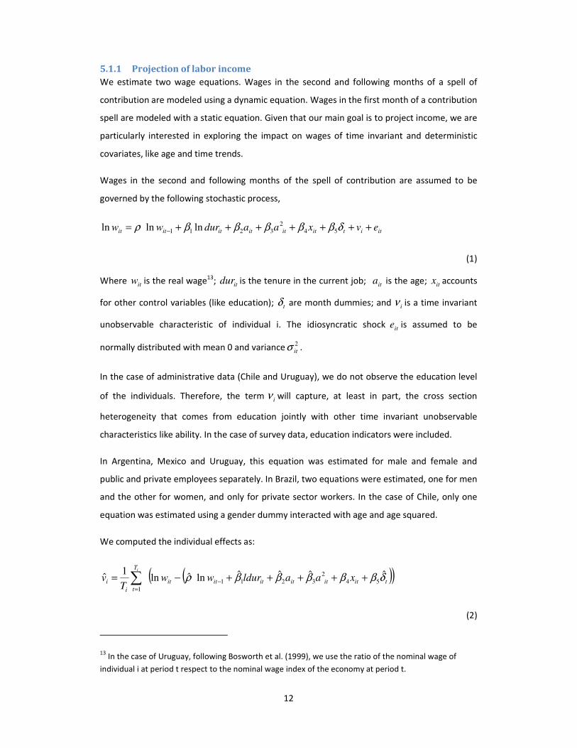
Wages in the second and following months of the spell of contribution are assumed to be
governed by the following stochastic process,
itititititititit evxaadurww +++++++= − δβββββρ54
2
3211lnlnln
(1)
Where itw is the real wage13
; itdur is the tenure in the current job; ita is the age; itx accounts
for other control variables (like education); tδ are month dummies; and iν is a time invariant
unobservable characteristic of individual i. The idiosyncratic shock ite is assumed to be
normally distributed with mean 0 and variance2
itσ .
In the case of administrative data (Chile and Uruguay), we do not observe the education level
of the individuals. Therefore, the term iν will capture, at least in part, the cross section
heterogeneity that comes from education jointly with other time invariant unobservable
characteristics like ability. In the case of survey data, education indicators were included.
In Argentina, Mexico and Uruguay, this equation was estimated for male and female and
public and private employees separately. In Brazil, two equations were estimated, one for men
and the other for women, and only for private sector workers. In the case of Chile, only one
equation was estimated using a gender dummy interacted with age and age squared.
We computed the individual effects as:
( )( )titititititit
T
ti
i xaaldurwwT
vi
δβββββρ ˆˆˆˆlnˆln1
ˆ54
2
3211
1
+++++−= −
=
∑
(2)
13 In the case of Uruguay, following Bosworth et al. (1999), we use the ratio of the nominal wage of
individual i at period t respect to the nominal wage index of the economy at period t.
13
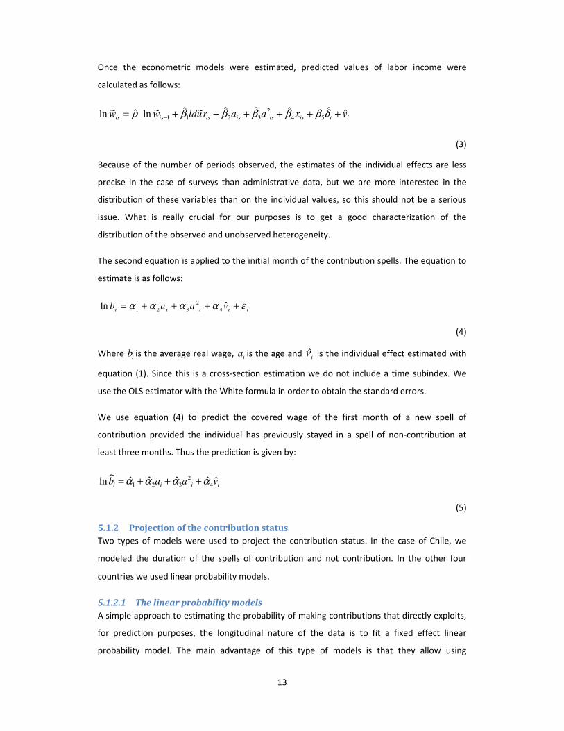
Once the econometric models were estimated, predicted values of labor income were
calculated as follows:
itisisisisisis vxaaruldww ˆˆˆˆˆ~ˆ~lnˆ~ln54
2
3211++++++= − δβββββρ
(3)
Because of the number of periods observed, the estimates of the individual effects are less
precise in the case of surveys than administrative data, but we are more interested in the
distribution of these variables than on the individual values, so this should not be a serious
issue. What is really crucial for our purposes is to get a good characterization of the
distribution of the observed and unobserved heterogeneity.
The second equation is applied to the initial month of the contribution spells. The equation to
estimate is as follows:
(4)
Where ib is the average real wage, ia is the age and iν̂ is the individual effect estimated with
equation (1). Since this is a cross-section estimation we do not include a time subindex. We
use the OLS estimator with the White formula in order to obtain the standard errors.
We use equation (4) to predict the covered wage of the first month of a new spell of
contribution provided the individual has previously stayed in a spell of non-contribution at
least three months. Thus the prediction is given by:
iiii vaab ˆˆˆˆˆ~
ln4
2
321αααα +++=
(5)
5.1.2 Projection of the contribution status
Two types of models were used to project the contribution status. In the case of Chile, we
modeled the duration of the spells of contribution and not contribution. In the other four
countries we used linear probability models.
5.1.2.1 The linear probability models
A simple approach to estimating the probability of making contributions that directly exploits,
for prediction purposes, the longitudinal nature of the data is to fit a fixed effect linear
probability model. The main advantage of this type of models is that they allow using
iiiii vaab εαααα ++++= ˆln4
2
321
14
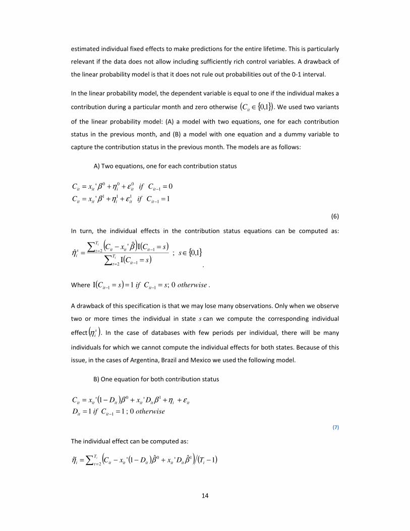
estimated individual fixed effects to make predictions for the entire lifetime. This is particularly
relevant if the data does not allow including sufficiently rich control variables. A drawback of
the linear probability model is that it does not rule out probabilities out of the 0-1 interval.
In the linear probability model, the dependent variable is equal to one if the individual makes a
contribution during a particular month and zero otherwise { }( )1,0∈itC . We used two variants
of the linear probability model: (A) a model with two equations, one for each contribution
status in the previous month, and (B) a model with one equation and a dummy variable to
capture the contribution status in the previous month. The models are as follows:
A) Two equations, one for each contribution status
1'
0'
1
111
1
000
=++=
=++=
−
−
ititiitit
ititiitit
CifxC
CifxC
εηβ
εηβ
(6)
In turn, the individual effects in the contribution status equations can be computed as:
( ) ( )
( ){ }1,0;
ˆ'ˆ
2 1
2 1∈
=Ι
=Ι−=
∑
∑
= −
= −s
sC
sCxC
i
i
T
t it
T
t ititits
i
βη
.
Where ( ) otherwisesCifsC itit 0;111
===Ι −− .
A drawback of this specification is that we may lose many observations. Only when we observe
two or more times the individual in state s can we compute the corresponding individual
effect ( )s
iη . In the case of databases with few periods per individual, there will be many
individuals for which we cannot compute the individual effects for both states. Because of this
issue, in the cases of Argentina, Brazil and Mexico we used the following model.
B) One equation for both contribution status
( )otherwiseCifD
DxDxC
itit
itiititititit
0;11
'1'
1
10
==
+++−=
−
εηββ
(7)
The individual effect can be computed as:
( )( ) ( )∑ =−+−−= iT
t iitititititi TDxDxC2
101ˆ'ˆ1'~ ββη
15
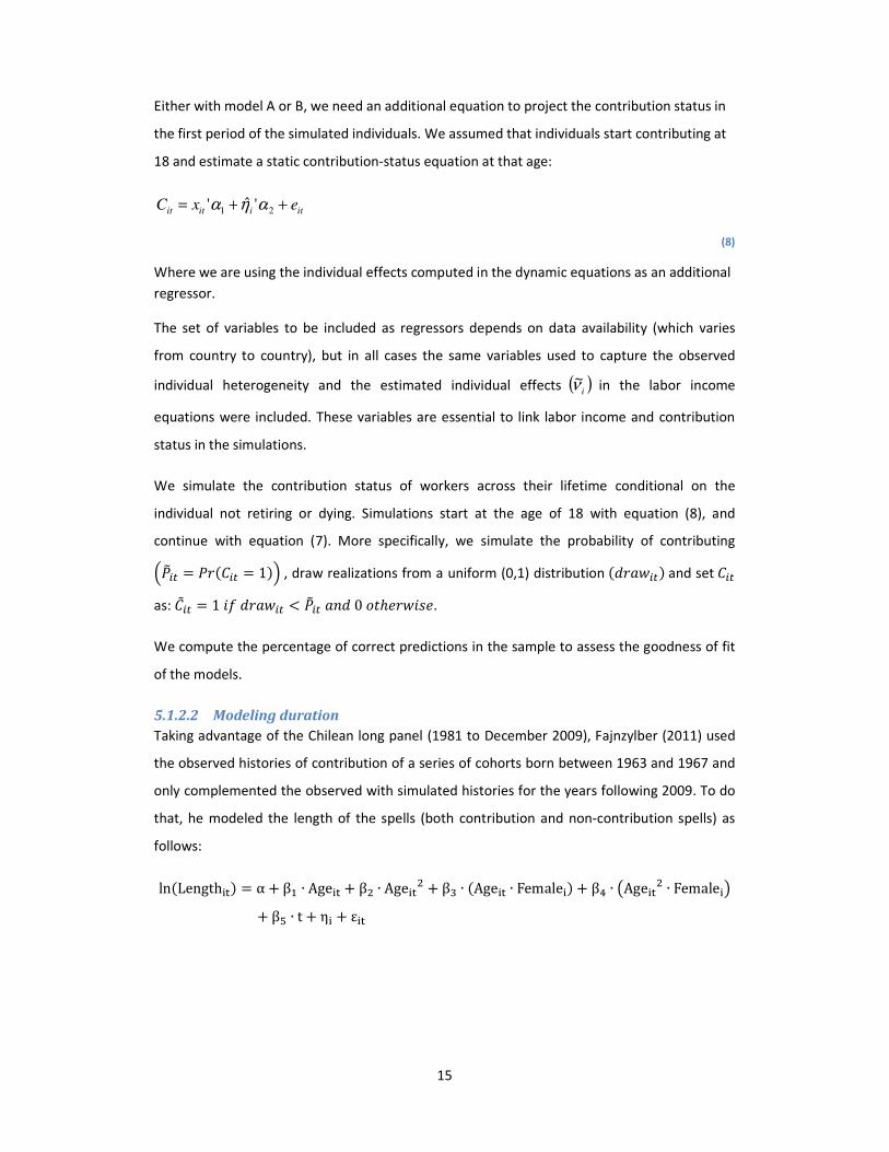
Either with model A or B, we need an additional equation to project the contribution status in
the first period of the simulated individuals. We assumed that individuals start contributing at
18 and estimate a static contribution-status equation at that age:
itiitit exC ++=21
'ˆ' αηα
(8)
Where we are using the individual effects computed in the dynamic equations as an additional
regressor.
The set of variables to be included as regressors depends on data availability (which varies
from country to country), but in all cases the same variables used to capture the observed
individual heterogeneity and the estimated individual effects ( )iν~ in the labor income
equations were included. These variables are essential to link labor income and contribution
status in the simulations.
We simulate the contribution status of workers across their lifetime conditional on the
individual not retiring or dying. Simulations start at the age of 18 with equation (8), and
continue with equation (7). More specifically, we simulate the probability of contributing
����� = ����� = 1�� , draw realizations from a uniform (0,1) distribution � ������ and set ��
as: ��� = 1 �� ����� < ���� �� 0 ��ℎ������.
We compute the percentage of correct predictions in the sample to assess the goodness of fit
of the models.
5.1.2.2 Modeling duration
Taking advantage of the Chilean long panel (1981 to December 2009), Fajnzylber (2011) used
the observed histories of contribution of a series of cohorts born between 1963 and 1967 and
only complemented the observed with simulated histories for the years following 2009. To do
that, he modeled the length of the spells (both contribution and non-contribution spells) as
follows:
ln�Length#$� = α + β( ∙ Age#$ + β+ ∙ Age#$+ + β, ∙ �Age#$ ∙ Female#� + β0 ∙ 1Age#$
+ ∙ Female#2+ β3 ∙ t + η# + ε#$
16
Where i indexes individuals, t indexes the spells of each individual and the variable Age is
measured at the beginning of the corresponding spell. The variable η# represents the individual
fixed effects.
5.2 Computation of SS contributions and benefits
Once we had the simulated work histories, we computed social security contributions,
unemployment benefits and pensions, according to the existing social security norms. This step
involves programming the current social security rules. We considered both employee and
employer contributions, as both eventually impact on net wages in the long run (Gruber, 1999,
p 90; Brown et al. 2009, p 13; Hamermesh and Rees 1993, p 212).
We considered two social security programs, old-age pensions and unemployment insurance.
Old-age, survival and disability (OASDI) benefits are usually integrated in a single program.
Unemployment insurance is often an independent program, but with important contributions
from the government. In the case of Uruguay, contributions to social security finance both
OASDI and unemployment insurance. Because of this, Forteza and Mussio (2011) modeled the
two programs together. Regarding OASDI benefits, we focused on old-age pensions, assuming
the simulated individuals leave no survivors and suffer no disability.
Individuals are assumed to claim benefits as soon as they are eligible. In the cases of Argentina
and Uruguay, a scenario in which vesting period conditions are not fully enforced was also
simulated. In this alternative scenario, individuals who claim and receive pensions without
having fulfilled the years of contribution legally required are assumed to receive minimum
pensions. The aim of simulating this weak enforcement scenario is twofold. First, we want to
assess the impact of vesting period conditions on social security progressiveness. Second, this
scenario is a stylized representation of actual practices in two social security programs in which
the testimony of witnesses to credit contributions is still common practice.
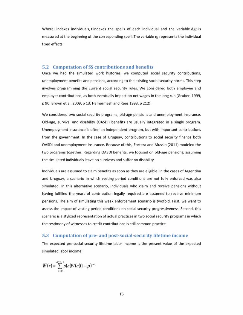
5.3 Computation of pre- and post-social-security lifetime income
The expected pre-social security lifetime labor income is the present value of the expected
simulated labor income:
( ) ( ) ( )( ) ara
a
aWaprW−
−=
=
+= ∑ ρ1
1
0
17
Where r is age at retirement, ( )ap is the probability of worker’s survival at age a , ( )aW is
labor income at age a , and ρ is the discount rate.
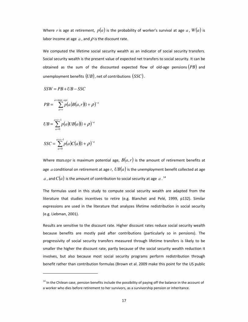
We computed the lifetime social security wealth as an indicator of social security transfers.
Social security wealth is the present value of expected net transfers to social security. It can be
obtained as the sum of the discounted expected flow of old-age pensions ( )PB and
unemployment benefits ( )UB , net of contributions ( )SSC .
SSCUBPBSSW −+=
( ) ( )( ) aagea
ra
raBapPB−
=
=
+= ∑ ρ1,
max
( ) ( )( ) ara
a
aUBapUB−
−=
=
+= ∑ ρ1
1
0
( ) ( )( ) ara
a
aCapSSC−
−=
=
+= ∑ ρ1
1
0
Where agemax is maximum potential age, ( )raB , is the amount of retirement benefits at
age a conditional on retirement at age r, ( )aUB is the unemployment benefit collected at age
a , and ( )aC is the amount of contribution to social security at age a . 14
The formulas used in this study to compute social security wealth are adapted from the
literature that studies incentives to retire (e.g. Blanchet and Pelé, 1999, p132). Similar
expressions are used in the literature that analyzes lifetime redistribution in social security
(e.g. Liebman, 2001).
Results are sensitive to the discount rate. Higher discount rates reduce social security wealth
because benefits are mostly paid after contributions (particularly so in pensions). The
progressivity of social security transfers measured through lifetime transfers is likely to be
smaller the higher the discount rate, partly because of the social security wealth reduction it
involves, but also because most social security programs perform redistribution through
benefit rather than contribution formulas (Brown et al. 2009 make this point for the US public
14 In the Chilean case, pension benefits include the possibility of paying off the balance in the account of
a worker who dies before retirement to her survivors, as a survivorship pension or inheritance.
18
social security program). We used a discount rate of 3 percent per annum (ppa), but Forteza
and Mussio (2011) and Moncarz (2011) performed sensitivity analysis for Uruguay and
Argentina respectively. For the US case, Brown et al. (2009) use 2 and 4 ppa. Liebman (2001)
uses the internal rate of return of the cohort he analyzes -1.29 ppa- in order to focus only on
intra-cohort redistribution.
Following our assumption of no behavioral responses, we assume that social security does not
impact on the age at retirement, so we used the same value of r to compute the pre- and
post-social security labor income. The only departure from this assumption is in the weak
enforcement scenario, in which all individuals retired at the minimum retirement age. Also, we
assumed that the interruptions in labor history are exogenously given, independent of the
unemployment insurance program.
5.4 Computation of income distribution indexes
We first characterize the distribution of individuals (i) social security wealth and (ii) social
security wealth to income ratios. These indicators provide a first assessment of how much
redistribution is taking place within the social security system.
Second, we plot individual social security wealth versus pre-social security labor income. This is
a first indicator of local progressiveness in social security redistribution. Liebman (2001)
presents similar plots for the US.
Third, we compute the Lorenz curves of the expected pre-social security labor income and the
associated concentration curves of the expected post-social security labor income (ranked by
pre-social security income).
Fourth, we compute the Ginis of the pre- and post-social security labor income and 95%
confidence intervals.
Finally, we compute the Reynolds-Smolensky-type index of net redistributive effect (Lambert,
1993, p 256). This index assesses the redistributive impact of a program computing the area
between the Lorenz pre-program income and the concentration post-program income. A
positive (negative) value indicates that the program reduces (increases) inequality.
The Lorenz and concentration curves, the Gini coefficients and the Reynolds-Somelinsky index
were estimated using DASP (Araar and Duclos 2009).
19
6 Results Estimations of the econometric models used to project labor income and contributions are not
presented in this paper. Readers interested in these intermediate results should look at the
background articles. The focus in this document is on the redistributive impact of the
programs. To that we turn now.
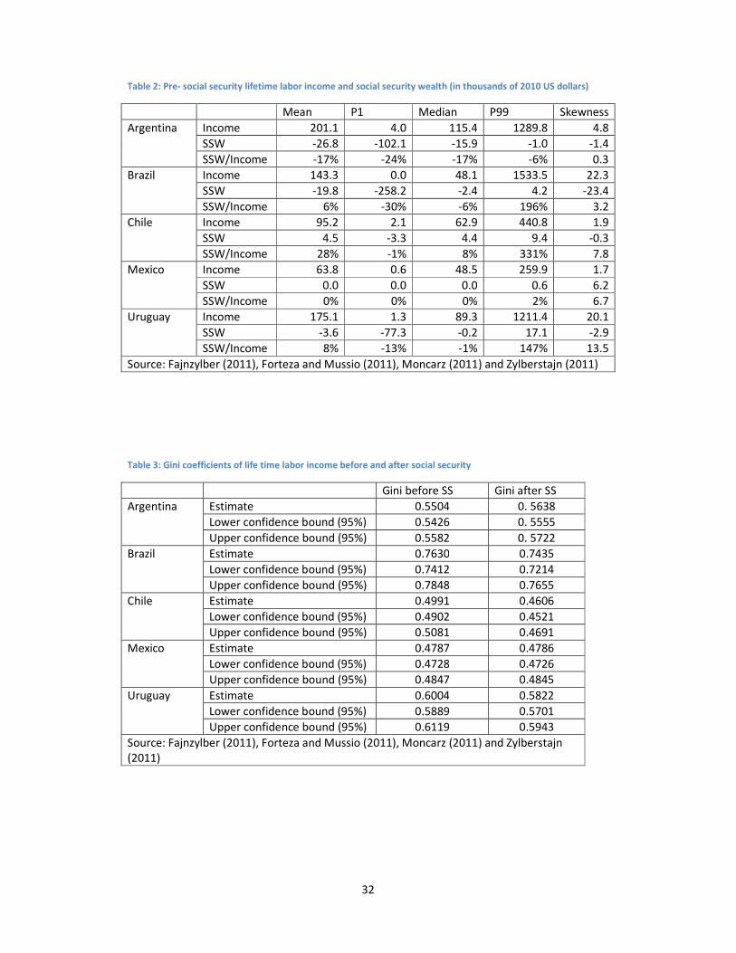
We present in Table 2 some descriptive statistics of the simulated databases. Average
expected life time income ranges from 64 thousand dollars in the Mexican to 199 thousand
dollars in the Argentinean databases. In the five countries, the simulated databases exhibit
much dispersion of income, which is crucial to effectively assess redistribution. There are some
simulated individuals with very low income. The percentile one individual (P1) has almost no
life time income in Brazil, partly due to small income when working but mostly due to very
short histories of contribution. The other countries exhibit higher P1 incomes, but even in
Argentina, which exhibits the highest P1 income, it is smaller than 4 thousand dollars. At the
other end of the distribution, the percentile 99 individuals (P99) range from 260 thousand
dollars in Mexico to more than 1,500 thousand dollars in Brazil. As expected, the distributions
are skewed to the right, with median consistently lower than mean income.
Average social security wealth ranges from minus 27 thousand dollars in Argentina to 4.5
thousand dollars in Chile. Measured by the difference between percentiles 1 and 99 within
each country, social security wealth exhibits more dispersion in Argentina, Brazil and Uruguay
than in Chile and Mexico. This is an expected result, since the Chilean and Mexican pensions
programs are based on individual accounts, while the Argentinean and Brazilian programs are
PAYG-DB and the Uruguayan program is mixed, but with a large proportion of PAYG-DB. The
Mexican social security system appears as almost actuarially neutral in these simulations. The
Chilean system looks much less neutral: the P1 and P99 social security wealth are minus 3.3
and plus 9.4 thousand dollars, respectively.
Brazil is the country that exhibits the largest dispersion in social security wealth in our study.
The P1 is as low as minus 258 thousand dollars. This large losses result from the lack of ceilings
on employers’ contributions combined with a maximum pension. Therefore, there is no lower
bound on social security wealth, since the higher the wage, the higher the implicit tax (and the
implicit redistribution). Argentina and Uruguay show much higher P1. Unlike in Brazil, because
of the existence of ceilings on insured wages, total contributions cannot be higher than certain
thresholds and social security wealth has a lower bound.

20
The distribution of social security wealth looks skewed to the left in Argentina, Brazil, Chile and
Uruguay and to the right in the Mexican system.
We also computed the expected social security wealth to life time income ratio for each
simulated individual. This indicator exhibits much dispersion between and within countries.
The average ratio ranges from – 17 percent in Argentina to + 28 percent in Chile. It is zero in
Mexico, 6 percent in Brazil and 8 percent in Uruguay.15
The social security wealth to income ratio exhibits almost no dispersion in the simulated
Mexican database. Therefore, according to these results, social security would not perform any
significant redistribution in expected terms in Mexico. This is not surprising in an individual
accounts program. Nevertheless, the other individual accounts program in our sample, Chile,
exhibits much more dispersion. Sorting individuals by the social security wealth to lifetime
income ratio, the P1 individual loses about 1 percent and the P99 individual gains 331 percent
of their lifetime income in Chile. So, despite of being based on individual accounts, the Chilean
system seems to have enough departure from actuarial neutrality as to perform significant
redistribution. The Argentinean program shows less dispersion in the ratio than other
programs covered in our study, apart from Mexico. However, the fact that the P1 individual
losses is as much as 24 percent of his lifetime income through social security indicates that we
cannot yet rule out significant redistribution from taking place within the Argentinean social
security system. The Brazilian and Uruguayan programs show much more variation in the ratio,
highlighting a potentially large redistribution.
According to our simulations, Argentina, Brazil, Chile and Uruguay exhibit considerable
variation in social security wealth and social security wealth to lifetime income ratios across
individuals, performing significant redistribution. This is not the case of Mexico. Whether this
potential is actually realized and what sign it has depends on how these transfers are
correlated to lifetime income. We turn now to this point.
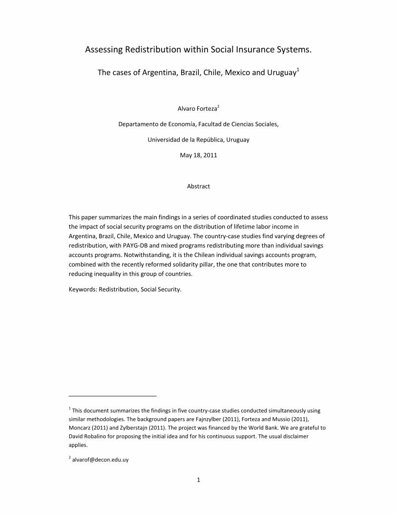
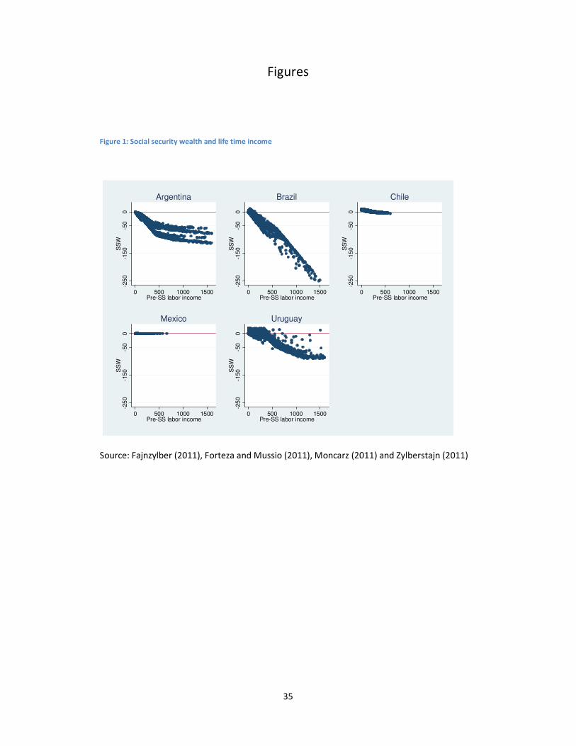
Figure 1 plots social security wealth and pre social security lifetime labor income. To facilitate
comparisons, we limited the range of values in the figure from the minimum P1 to the
maximum P99 in the set of countries. It should be noticed that in the case of Brazil individuals
with income above P99 would have social security wealth smaller than the highly negative
15 Liebman (2001) computed the same indicator for the United States. Using a discount rate of 3 percent
per annum -the same rate used in the present study-, he finds the average ratio to be -6.6%.

21
value observed in the figure. Instead, in the cases of Argentina and Uruguay, higher income
workers do not get more negative social security wealth, because as explained before they
have already reached the lower bound.
The negative slope of the plots suggests that the PAYG Argentinean and Brazilian programs
and the mixed Uruguayan program are progressive, while the flat plots of the individual
accounts Chilean and Mexican programs suggest much more neutrality. Actually, there is
redistribution at the lower end of the distribution in the Chilean and Mexican programs, but
when the scale of the graphs is unified to facilitate cross-country comparisons as we did in this
figure, the plots of the individual accounts programs look flat compared to the plots of the
PAYG and mixed programs.
Figure 1 also shows considerable variability of social security wealth for each level of lifetime
labor income in Argentina, Brazil and Uruguay. Therefore, there seems to be some
redistribution that is not correlated to income levels in the PAYG and mixed programs covered
in this study. Liebman (2001) reports a similar finding for the US.
These observations suggest that while the individual account programs perform less
redistribution on average than the PAYG programs, they might be better targeted regarding
redistribution. The net impact of the programs on the distribution of post-social security life
time income is thus not a priori obvious.
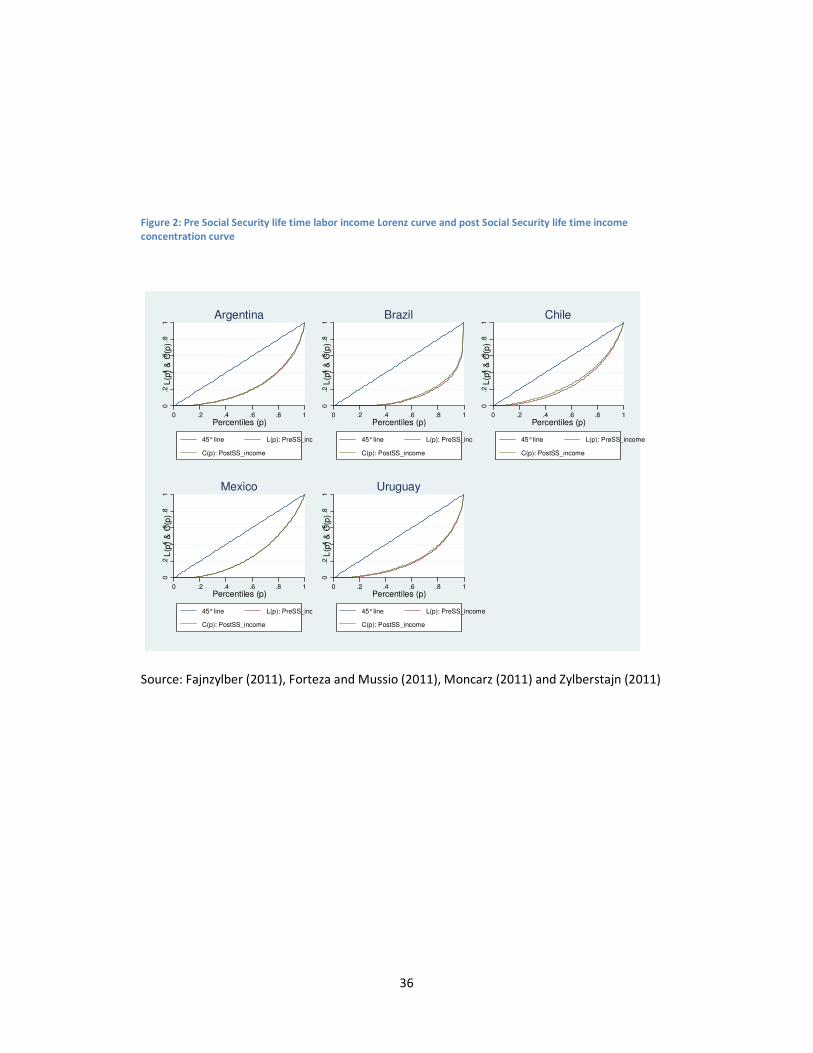
Figure 2 presents the Lorenz curves of pre social security labor income and the concentration
curves of post social security labor income. We do not observe large differences between the
pre and post social security curves in these countries. Brazil and Chile are the only cases in
which there seems to be an observable equalizing effect of social security.
The Gini coefficients of the simulated pre social security life time labor income range from a
minimum of 0.48 in Mexico to a maximum of 0.76 in Brazil (Table 3). According to this
indicator, the distribution of the income measure considered in the present study is much
more unequal than the distribution of current household per capita income reported to
household surveys in Argentina, Brazil and Uruguay and more equal in Chile and Mexico.16
16 CEDLAS and The World Bank (April 2011), for example, report Gini coefficients estimated on 2009
household per capita income of: 0.449 for Argentina, 0.537 for Brazil, 0.519 for Chile, 0.505 for Mexico
and 0.44 for Uruguay. These indicators are not directly comparable to ours though. The Ginis reported in
the present study refer to individual income as opposed to household per capita income, to labor as
opposed to total income, to formal (in the sense of reported to social security) as opposed to formal

22
Brazil is the most unequal in this group of countries according to both estimations, but the
ranking regarding other countries differs considerably. We do not want to push the
comparative perspective further, though, not only because the definition of income used in
these studies is very different, but also because data sources used to compute life time income
in the five countries covered in our project are also different (short panel surveys in Argentina,
Brazil and Mexico and administrative records in Chile and Uruguay). More research on the
distribution of life time labor income declared to social security is needed. With this caveat in
mind, we turn now to our estimations of the impact of social security on inequality.
According to our estimations, Chile is the country in which social security causes the largest
reduction in inequality (Table 3 and Table 4). The point estimation of the Gini coefficient is
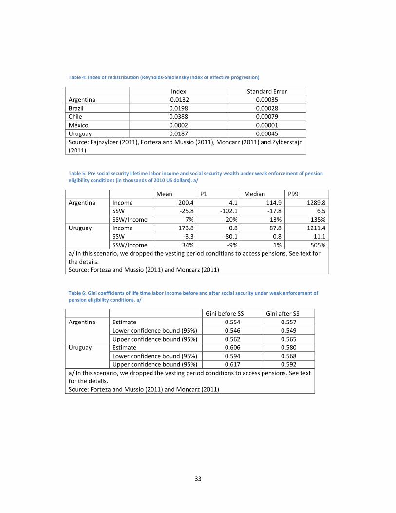
reduced by almost four points and the 95% confidence intervals do not overlap. The Reynolds-
Smolenski index (RS) of effective progression is almost 4 percentage points and is significant at
1%.The second largest fall in the Gini coefficient due to social security in our study takes place
in Brazil, where we see a two point fall, and the third in Uruguay, with a 1.8 point fall. The RS
index is in the order of 2 percentage points and highly significant both in Brazil and Uruguay.
Mexico shows almost no change in the Gini coefficients. The RS index is 0.02 percentage
points. Finally, Argentina shows a 1.3 point increase in the Gini coefficient due to social
security, with a small overlap of the 95% confidence intervals. The RS index is -1.3 percentage
points and is significant at 1%.
The reduction in income inequality that the Chilean social security system performs is
remarkable. It is a system based on mostly actuarially neutral individual savings accounts, and
as such produces much less redistribution than the PAYG and mixed programs analyzed in
Argentina, Brazil and Uruguay. The difference between the P99 and P1 social security wealth is
more than 90 thousand dollars in Argentina and Uruguay, and more than 260 thousand dollars
in Brazil, but only 13 thousand dollars in Chile. And yet, the Chilean program is the one that
shows the largest fall in income inequality in the countries studied. This result suggests that
redistribution in the Chilean pension program is much better targeted than in the other four
countries. The limited but well targeted redistribution in this social security system rests on the
combination of a mostly actuarially neutral savings account and a relatively small but well
targeted solidarity complement.
plus informal income, and to simulated expected lifetime as opposed to reported current income. Also,
in the case of Brazil, only private sector workers are included.

23
In addition, it is not surprising that the Mexican social security system does not impact on
income distribution. Descriptive statistics of the social security wealth showed very small
values, consistent with a mostly actuarially neutral program. Minimum pensions and
government matching contributions represent departures from actuarial neutrality in the
Mexican social security system, but the size of these deviations is not enough to significantly
impact on income distribution.
The failure of the Argentinean and, to a lesser extent, the Uruguayan social security programs
to reduce inequality represents a puzzle. Vesting period conditions might help explain the
puzzle. In Argentina and Uruguay ordinary pensions can be claimed after thirty years of
contribution, a condition that many contributors do not seem to be able to fulfill. Forteza et al.
(2009) show that large segments of the population have a low probability of having
contributed thirty or more years when they reach retirement ages, and this probability is
particularly low among low income individuals. In turn, Forteza and Ourens (2011) show that
the implicit rate of return on contributions paid to these programs is very low when individuals
have short contribution histories. Hence, low income individuals might be getting a bad deal
from social security because they have short histories of contribution.
In order to test this hypothesis, Moncarz (2011) and Forteza and Mussio (2011) simulated an
additional scenario in which the vesting period condition is not required in practice. In this
“weak enforcement” scenario, the social security administration does not control whether
individuals have contributed the required thirty years to get an ordinary pension at the
minimum retirement age. The assumption is that everybody can claim an ordinary pension at
that age. Individuals who did not contribute thirty or more years at that age receive the
minimum pension. This scenario is not only useful to see whether vesting period conditions
could be behind the redistributive puzzle, but also to get closer to actual practice in weak
institutional environments in which the testimony of witnesses to credit periods of
contribution to social security is still common practice. The results of this scenario are
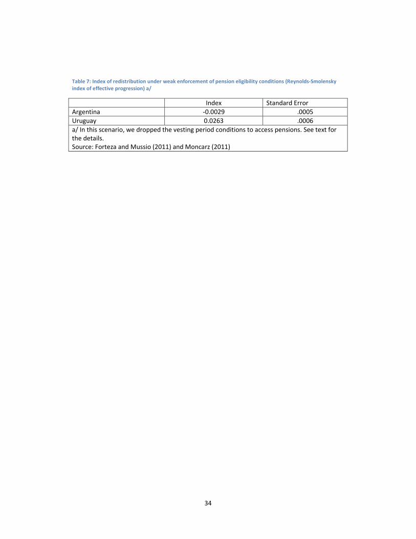
summarized in Table 6, Table 7 and Figure 3.
Social security looks more progressive in the weak than in the strict enforcement scenario. In
Uruguay, social security causes a 2.6 points fall in the Gini coefficient in the weak against 1.7 in
the strict enforcement scenario. The RS is now 2.6 percentage points. An increase in the social
security wealth of low income individuals seems to be behind the improvement (Figure 3). In
Argentina, social security still fails to reduce inequality in the weak enforcement scenario. The
Gini coefficient does not increase as much as in the base case scenario, but post-social security
24
income still exhibits higher Gini than pre-social security income and the RS index is negative
and significant at the usual levels.
Moncarz (2011) for Argentina and Forteza and Mussio (2011) for Uruguay run additional
simulations with lower discount rates. Social security looks more redistributive when flows are
discounted at lower interest rates, but the main results do not change qualitatively. In the case
of Argentina, only in the scenario with weak enforcement and 1 percent interest rate (the
lowest rate used) did social security significantly reduce inequality.
Fajnzylber (2011) assesses the separate impact of unemployment insurance and old age
pension programs on the distribution of income in Chile. He finds that unemployment
insurance is progressive. Most individuals have negative expected life time net transfers to this
program, but individuals at the bottom of income distribution have positive net transfers due
to the solidarity fund. Higher income individuals are less likely to benefit from this fund
because (i) they are less exposed to unemployment and (ii) when unemployed they are less
likely to be eligible for the solidarity funds benefits, because the balances in their individual
accounts tend to exceed the maximum level to be eligible for these benefits.
Notwithstanding, the unemployment insurance program has a limited impact on income
distribution. Fajnzylber (2011) reports a Reynolds-Smolenski index of redistributive effect of
0.097 for this program, as opposed to 3.876 for the joint effect of unemployment insurance
and old-age pensions. The main reason behind this is the relatively small size of the
unemployment insurance program.
7 Concluding Remarks The studies summarized in this document show that much redistribution is taking place
through the social security systems in Argentina, Brazil, and Uruguay, very little in Mexico and
something in between in Chile. Life time redistribution was measured simulating histories of
contribution and computing benefits and individual expected life time net transfers to social
security (i.e. the individuals’ social security wealth). The amount of redistribution was assessed
computing the dispersion of the social security wealth and the social security wealth to pre
social security income ratios. The difference between the percentiles 99 and 1 of social
security wealth is about 260 thousand dollars in Brazil, 90 thousand dollars in Argentina and
Uruguay, 13 thousand in Chile and 0.5 thousand dollars in Mexico. As expected, the two
individual accounts programs (Chile and Mexico) exhibit much less redistribution than the
PAYG and mixed programs (Argentina, Brazil and Uruguay).
25
However, the net impact of social security on the distribution of income is not directly aligned
to the size of total redistribution. Chile is the country in which the social security system makes
the largest contribution to reducing inequality, despite of having the second smallest
dispersion in social security wealth in our sample of countries. Fajnzylber (2011) reports an
almost four points reduction in the Gini coefficient in Chile, as compared to about two points
reduction in Brazil (Zylberstajn, 2011) and Uruguay (Forteza and Mussio, 2011), no changes in
Mexico, and an almost two points increase in Argentina (Moncarz, 2011).
The results summarized in this document suggest that the Chilean program has less but better
targeted redistribution than the Argentinean, Brazilian and Uruguayan programs: with less
total redistribution it performs a larger reduction in inequality. The Brazilian and Uruguayan
programs look quite progressive, but not as much as the Chilean one and much of the
redistribution they cause does not seem to be contributing to reducing inequality. The
Mexican program does not seem to redistribute much. The Argentinean program is the most
puzzling: it performs much redistribution, but it fails to reduce inequality, and it might even
exacerbate it.
8 References
Araar, A. and J.-Y. Duclos (2009). DASP: Distributive Analysis Stata Package, University of Labat, PEP,
World Bank, UNDP.
Amarante, V. and M. Bucheli (2008). "Análisis del seguro de desempleo en Uruguay y discusión
de propuestas para su modificación." Cuadernos del CLAEH 31(1-2): 175-207.
Auerbach, A. and L. Kotlikoff. 1987. Dynamic Fiscal Policies. Cambridge University Press.
Barreto de Oliveira, F. and K. Iwakami Beltrão (2002). The Brazilian Social Security System.
Institudo de Pesquisa Económica Aplicada, Ministério do Planejamento, Orçamento e Gestão.
Rio de Janeiro: 20.
Beach, W. and Davis, G. 1998. "Social Security's Rate of Return," CDA 98-01. Heritage
Foundation, vol. 21.
Berstein, S., G. Larraín, and F. Pino. 2006. "Chilean Pension Reform: Coverage Facts and Policy
Alternatives." Economía. vol.6, issue 2: 227-279.
Blanchet, Didier and Louis-Paul Pelé. 1999. Social Security and Retirement in France. In:
Gruber, J. and D. Wise, Social Security and Retirement around the World. NBER.
26
Boldrin, Michele; Jiménez-Martín, Sergi and Peracchi, Franco. 1999. "Social Security and
Retirement in Spain," J. Gruber and D. A. Wise, Social Security and Retirement around the
World. Chicago and London: The University of Chicago Press,
Boldrin, Michele; Jiménez-Martín, Sergi and Peracchi, Franco. 2004. "Micro-Modelling of
Retirement Behavior in Spain," J. Gruber and D. A. Wise, Social Security Programs and
Retirement around the World. Chicago: 499-578.
Bosworth, B., G. Burtless, M. Favreault, J. O’Hare, C. Ratcliffe, K. Smith, E. Toder, and C.
Uccello. 1999. "Modeling Income in the near Term - Projections of Retirement Income through
2020 for the 1931-60 Birth Cohorts." Washington DC. The Brookings Institution.
Brown, Jeffrey R.; Julio Lynn Coronado and Don Fullerton. “Is Social Security Part of the Social
Sefety Net?” NBER WP 15070. 2009.
CEDLAS and The World Bank (2011): Socio-Economic Database for Latin America and the
Caribbean SEDLAC. http://sedlac.econo.unlp.edu.ar/eng/index.php.
Diamond, P. 2005. “Taxation, Incomplete Markets, and Social Security”. The MIT Press.
Duggan, J., R. Gillingham and J. Greenlees. 1995. “Progressive Returns to Social Security? An
Answer from Social Security Records.” Washington DC, Office of Economic Policy, U. S.
Department of the Treasury. Office of Prices and Living Conditions. U.S. Bureau of Labor
Statistics, Research Paper 9501.
Fajnzylber, Eduardo (2011). Implicit Redistribution in the Chilean Social Insurance System.
Working Paper. Universidad Alberto Ibáñez. Chile. April.
Ferrer, A. M. and W. C. Riddell (2009). Unemployment Insurance Savings Accounts in Latin
America: Overview and Assessment. Social Protection Discussion Papers, The World Bank.
Forteza, A. 2007: Efectos distributivos de la reforma de la seguridad social. El caso uruguayo.
Cuadernos de Economía, Vol 44 (Mayo) pp 31-58.
Forteza, Alvaro; Ignacio Apella; Eduardo Fajnzylber; Carlos Grushka; Ianina Rossi and Graciela
Sanroman. 2009. Work Histories and Pension Entitlements in Argentina, Chile and Uruguay, SP
Discussion Papers Nº 0926, World Bank.
Forteza, Alvaro and Irene Mussio (2011). Assessing Redistribution in the Uruguayan Social
Security System. Working Paper. dECON-FCS-Universidad de la República. Uruguay. April.
Forteza, Alvaro and Guzmán Ourens (2011). Redistribution, Insurance and Incentives to Work
in Latin American Pension Programs. Working Paper. dECON-FCS-Universidad de la República.
Uruguay. April.
Forteza, A. and I. Rossi (2009). "The Contribution of Government Transfer Programs to
Inequality. A Net Benefit Approach." Journal of Applied Economics 12(1): 55-67.
Garrett, D. 1995. “The Effects of Differential Mortality Rates on the Progressivity of Social
Security,” Economic Inquiry, vol. 33: 457-75.
27
Gustman, Alan I. and Steinmeier, Thomas L. 2001. "How Effective Is Redistribution under the
Social Security Benefit Formula?" Journal of Public Economics, 82(1), pp. 1-28.
Gruber, Jonathan and David A. Wise eds. 1999. Social Security and Retirement Around the
World. Chicago and London: The University of Chicago Press.
Gruber, Jonathan, 1999, Social Security and Retirement in Canada. En: Gruber, Jonathan and
David A. Wise eds. 1999. Social Security and Retirement Around the World. Chicago and
London: The University of Chicago Press. Pages 73-100.
Gruber, Jonathan and David A. Wise eds. 2004. Social Security and Retirement Around the
World. Microestimations. Chicago and London: The University of Chicago Press.
Hamermesh, Daniel S. and Albert Rees. 1993. The Economics of Work and Pay. New
York: Harper Collins College Publishers.
Huff Stevens, A. 1999. "Climbing out of Poverty, Falling Back In: Measuring the Persistence of
Poverty over Multiple Spells," Journal of Human Resources 34(3) (Summer): 557-88.
Huggett, Mark and Ventura, Gustavo. "Sobre Los Efectos Distributivos De La Reforma De La
Seguridad Social." Cuadernos Económicos de I.C.E., 2000, 64, pp. 75-108.
Jiménez-Martín, Sergi and Sánchez Martín, Alfonso R. 2007. "An Evaluation of the Life Cycle
Effects of Minimum Pensions on Retirement Behavior." Journal of Applied Econometrics, 22(5),
pp. 923-50.
Lambert, Peter, 1993, The Distribution and Redistribution of Income. Manchester University
Press. 2nd edition.
Liebman, J. (2001). Redistribution in the Current US Social Security System. NBER Working
Paper Series, WP8625. Cambridge, MA.
Moncarz, Pedro (2011). Assessing Implicit Redistribution in the Argentinean and Mexican
Social Security Systems. Working Paper. Universidad de Córdoba. Argentina. April.
Morató, A. I. and A. Musto (2010). El impacto de la tasa de dependencia y de la antigüedad en
los rendimientos de los regímenes jubilatorios. Facultad de Ciencias Económicas y de
Administración. Montevideo, Universidad de la República.
Ochoa León, S. M. (2005). El seguro de desempleo en México y el mundo. Centro de Estudios
Sociales y de Opinión Pública.
RIBAS, Rafael Perez and SOARES. 2010. Sergei Suarez Dillon. O atrito nas pesquisas
longitudinais: o caso da pesquisa mensal de emprego (PME/IBGE). Estud. Econ. [online].
vol.40, n.1, pp. 213-244. ISSN 0101-4161. doi: 10.1590/S0101-41612010000100008
Rofman, Rafael; Lucchetti, Leonardo and Ourens, Guzmán. 2008. "Pension Systems in Latin
America: Concepts and Measurements of Coverage," Social Protection Discussion Papers.
Washington DC.

28
Sutherland, Holly. 2001. "Euromod: An Integrated European Benefit-Tax Model," Euromod,
119.
Velásquez, M. (2010). Seguros de desempleo y reformas recientes en América Latina, CEPAL.
Zylberstajn, Eduardo (2011). Assessing Implicit Redistributrion in the Brazilian Social Security
System. Working Paper. Fundação Getúlio Vargas. Brazil. April.
29
Tables
Table 1: Main parameters in the old-age pension programs
Program Contributions a/ Qualifying conditions Benefits
Argentina
( PAYG-DB )
Employee: 11.00%
Employer: 16.00%
Men: �7� ≥ 65 & <�� ≥ 30
Women: �7� ≥ 60 & <�� ≥ 30
�>? + "A ������<"
Minimum pension = 265 dollars (end of 2010)
Where:
�>? = 125 �<<��� ��� �� 2010�
"A ������<" = 0.015 × E���35, <��� × �G
�7� ≥ 70 & 30 > <�� ≥ 10
(with at leat 5 years of contributions
during the 8 years previous to retire)
0.7 × �>? + "A ������<"
Brazil
( PAYG-DB )
Employee: 8 to 11%.
Employer: 20%.
a) "Length of service":
Men: <�� ≥ 35
Women: <�� ≥ 30
= �G ∗ "����� K��L� ��M�����"
Note: the “fator previdenciario” is a decreasing
function of life expectancy at retirement.
b) "Advanced age":
Men: �7� ≥ 65 & <�� ≥ 15
Women: �7� ≥ 60 & <�� ≥ 15
= 0.7�1 + 0.01<����G ≤ �G
30
Program Contributions a/ Qualifying conditions Benefits
Chile
(Individual accounts
plus “solidarity” pillar)
Employee: 13.04%
(10% individual account + 1.49%
disability and insurance premium
+ 1.55% average administrative
fee, as of April 2011)
(Employers with more than 100
workers pay the 1.49% D&I
premium)
O��: �7� ≥ 65
Q�E�� �7� ≥ 60 ��
���R��S ≥ 0.7�G &
���R��S ≥ 1.5 × O��. ���.
Annuity + "solidarity complement"
Note: “solidarity complement” is reduced with the
level of the annuity and becomes zero if ���R��S ≥ �OAT, where PMAS is the Maximum
Pension with Solidarity Complement
Mexico
(Individual accounts plus
minimum pension and
government flat
contributions)
Employee: 1.125%
Employer: 5.15%
Government: 0.225% + flat
contribution for each day of
contribution (decreasing in
the wage rate)
�7� ≥ 65 & <�� ≥ 25 ��
���R��S ≥ 1.3E��K��
���R��S ≥ E��K��
Uruguay
(Mixed program:
(i) first tier: PAYG-DB;
(ii) second tier:
individual accounts)
Employee: 15%
Employer: 7.5%
�7� ≥ 60 & <�� ≥ 30 �� × �G
With: 0.45 ≤ �� ≤ 0.825
�7� ≥ 70 & <�� ≥ 15 �� × �G
With: 0.5 ≤ �� ≤ 0.65
�7� ≥ 65 ��
�7� ≥ 60 & <�� ≥ 30
Annuity
Notes: age = age when pension is claimed, in years; los = length of service when pension is claimed, in years; �G = average wage (wages
included in this average vary considerably between programs) ; E��K�� = minimum pension.
a/ In most programs, contributions to old age, survivor and disability insurance (OASDI) cannot be separated into three distinct
31
Program Contributions a/ Qualifying conditions Benefits
components. We report OASDI contributions in all cases. In Uruguay, contributions to old-age pensions and unemployment
insurance are bunched together.
Source: Author’s elaboration based on Forteza and Ourens (2011) .
32
Table 2: Pre- social security lifetime labor income and social security wealth (in thousands of 2010 US dollars)
Mean P1 Median P99 Skewness
Argentina Income 201.1 4.0 115.4 1289.8 4.8
SSW -26.8 -102.1 -15.9 -1.0 -1.4
SSW/Income -17% -24% -17% -6% 0.3
Brazil Income 143.3 0.0 48.1 1533.5 22.3
SSW -19.8 -258.2 -2.4 4.2 -23.4
SSW/Income 6% -30% -6% 196% 3.2
Chile Income 95.2 2.1 62.9 440.8 1.9
SSW 4.5 -3.3 4.4 9.4 -0.3
SSW/Income 28% -1% 8% 331% 7.8
Mexico Income 63.8 0.6 48.5 259.9 1.7
SSW 0.0 0.0 0.0 0.6 6.2
SSW/Income 0% 0% 0% 2% 6.7
Uruguay Income 175.1 1.3 89.3 1211.4 20.1
SSW -3.6 -77.3 -0.2 17.1 -2.9
SSW/Income 8% -13% -1% 147% 13.5
Source: Fajnzylber (2011), Forteza and Mussio (2011), Moncarz (2011) and Zylberstajn (2011)
Table 3: Gini coefficients of life time labor income before and after social security
Gini before SS Gini after SS
Argentina Estimate 0.5504 0. 5638
Lower confidence bound (95%) 0.5426 0. 5555
Upper confidence bound (95%) 0.5582 0. 5722
Brazil Estimate 0.7630 0.7435
Lower confidence bound (95%) 0.7412 0.7214
Upper confidence bound (95%) 0.7848 0.7655
Chile Estimate 0.4991 0.4606
Lower confidence bound (95%) 0.4902 0.4521
Upper confidence bound (95%) 0.5081 0.4691
Mexico Estimate 0.4787 0.4786
Lower confidence bound (95%) 0.4728 0.4726
Upper confidence bound (95%) 0.4847 0.4845
Uruguay Estimate 0.6004 0.5822
Lower confidence bound (95%) 0.5889 0.5701
Upper confidence bound (95%) 0.6119 0.5943
Source: Fajnzylber (2011), Forteza and Mussio (2011), Moncarz (2011) and Zylberstajn
(2011)
33
Table 4: Index of redistribution (Reynolds-Smolensky index of effective progression)
Index Standard Error
Argentina -0.0132 0.00035
Brazil 0.0198 0.00028
Chile 0.0388 0.00079
México 0.0002 0.00001
Uruguay 0.0187 0.00045
Source: Fajnzylber (2011), Forteza and Mussio (2011), Moncarz (2011) and Zylberstajn
(2011)
Table 5: Pre social security lifetime labor income and social security wealth under weak enforcement of pension
eligibility conditions (in thousands of 2010 US dollars). a/
Mean P1 Median P99
Argentina Income 200.4 4.1 114.9 1289.8
SSW -25.8 -102.1 -17.8 6.5
SSW/Income -7% -20% -13% 135%
Uruguay Income 173.8 0.8 87.8 1211.4
SSW -3.3 -80.1 0.8 11.1
SSW/Income 34% -9% 1% 505%
a/ In this scenario, we dropped the vesting period conditions to access pensions. See text for
the details.
Source: Forteza and Mussio (2011) and Moncarz (2011)
Table 6: Gini coefficients of life time labor income before and after social security under weak enforcement of
pension eligibility conditions. a/
Gini before SS Gini after SS
Argentina Estimate 0.554 0.557
Lower confidence bound (95%) 0.546 0.549
Upper confidence bound (95%) 0.562 0.565
Uruguay Estimate 0.606 0.580
Lower confidence bound (95%) 0.594 0.568
Upper confidence bound (95%) 0.617 0.592
a/ In this scenario, we dropped the vesting period conditions to access pensions. See text
for the details.
Source: Forteza and Mussio (2011) and Moncarz (2011)
34
Table 7: Index of redistribution under weak enforcement of pension eligibility conditions (Reynolds-Smolensky
index of effective progression) a/
Index Standard Error
Argentina -0.0029 .0005
Uruguay 0.0263 .0006
a/ In this scenario, we dropped the vesting period conditions to access pensions. See text for
the details.
Source: Forteza and Mussio (2011) and Moncarz (2011)
35
Figures
Figure 1: Social security wealth and life time income
Source: Fajnzylber (2011), Forteza and Mussio (2011), Moncarz (2011) and Zylberstajn (2011)
-25
0-1
50
-50
0S
SW
0 500 1000 1500Pre-SS labor income
Argentina
-25
0-1
50
-50
0S
SW
0 500 1000 1500Pre-SS labor income
Brazil
-25
0-1
50
-50
0S
SW
0 500 1000 1500Pre-SS labor income
Chile
-25
0-1
50
-50
0S
SW
0 500 1000 1500Pre-SS labor income
Mexico
-25
0-1
50
-50
0S
SW
0 500 1000 1500Pre-SS labor income
Uruguay
36
Figure 2: Pre Social Security life time labor income Lorenz curve and post Social Security life time income
concentration curve
Source: Fajnzylber (2011), Forteza and Mussio (2011), Moncarz (2011) and Zylberstajn (2011)
0.2
.4.6
.81
L(p
) &
C(p
)
0 .2 .4 .6 .8 1
Percentiles (p)
45° line L(p): PreSS_income
C(p): PostSS_income
Argentina0
.2.4
.6.8
1L
(p)
& C
(p)
0 .2 .4 .6 .8 1
Percentiles (p)
45° line L(p): PreSS_income
C(p): PostSS_income
Brazil
0.2
.4.6
.81
L(p
) &
C(p
)
0 .2 .4 .6 .8 1
Percentiles (p)
45° line L(p): PreSS_income
C(p): PostSS_income
Chile
0.2
.4.6
.81
L(p
) &
C(p
)
0 .2 .4 .6 .8 1Percentiles (p)
45° line L(p): PreSS_income
C(p): PostSS_income
Mexico
0.2
.4.6
.81
L(p
) &
C(p
)
0 .2 .4 .6 .8 1Percentiles (p)
45° line L(p): PreSS_income
C(p): PostSS_income
Uruguay
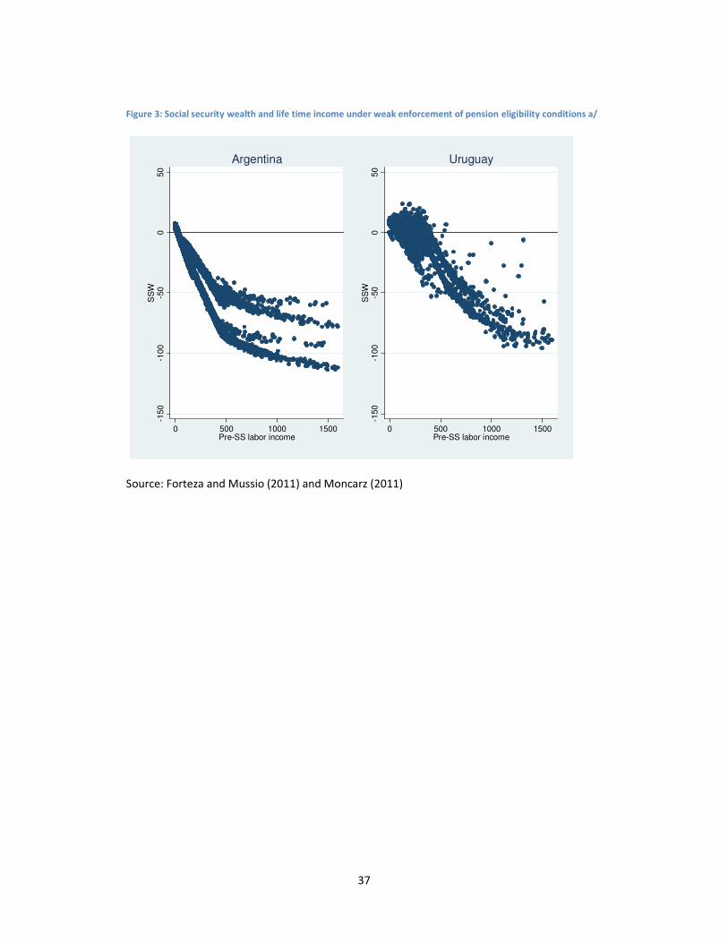
37
Figure 3: Social security wealth and life time income under weak enforcement of pension eligibility conditions a/
Source: Forteza and Mussio (2011) and Moncarz (2011)
-150
-100
-50
050
SS
W
0 500 1000 1500Pre-SS labor income
Argentina
-150
-100
-50
050
SS
W
0 500 1000 1500Pre-SS labor income
Uruguay