Assessing the Geographic Representativity of Farm Accountancy Data:Opportunities for new FADN Changes

Stuart Green, Cathal O’Donoghue and Brian Moran

Paper prepared for presentation at the 150th EAAE Seminar

“The spatial dimension in analysing the linkages between agriculture, ruraldevelopment and the environment”

Jointly Organised between Scotland’s Rural College (SRUC) and Teagasc

Scotland’s Rural College, Edinburgh, ScotlandOctober 22-23, 2015

Copyright 2015 by Stuart Green, Cathal O’Donoghue and Brian Moran. All rightsreserved. Readers may make verbatim copies of this document for non-commercial

purposes by any means, provided that this copyright notice appears on all such copies.

Assessing the Geographic Representativity of FarmAccountancy Data: Opportunities for new FADN Changes

Stuart Green*, Cathal O’Donoghue and Brian Moran

Rural Economy and Development Programme, Teagasc, Ireland

* Author to whom correspondence should be addressed; E-Mail: Stuart Green

Abstract: This is the abstract section. One paragraph only (Maximum 200 words). The

environment both affects agricultural production, via soils, weather, water availability etc

and agriculture affects the environment via its impact locally on landscape, water, soil

nutrition and biodiversity and more widely via its impact on climate change. Locating

agriculture within its spatial environment is thus very important in making decisions by

farmers, policy makers and other stakeholders. Within the EU, countries collect detailed

farm data to understand the technical and financial performance of farms as part of the

Farm Accountancy Data Network. However knowledge of the spatial-environmental

context of these farms is very limited as the spatial location of farms within these surveys

is very limited. In this paper we develop a methodology to geo-reference farms in this data.

We chose Ireland as a case study as the dominant farm systems are pasture based mainly

animal systems. Thus the local environment is particularly relevant to output. Agriculture

in Ireland is also amongst the largest as a proportion of the size of the economy and thus

the environmental impact is likely to be more important.

Applying this methodology has a number of challenges because Ireland does not have a

system of post codes. In addition there are complications in relation to place names which

may be in English or Irish or indeed a combination, often with non harmonised spellings

and often with non-unique place names. The methodology we develop in this paper

overcomes these difficulties allowing us to link, using resulting GIS coordinates, localised

environmental to the individual farm data. The primary objective of the survey is to

provide a nationally representative picture of farm outputs and outcomes. As a result the

survey may not necessarily be representative spatially or the pattern of environment x farm

system. Within the paper we assess the relative spatial representativity.

Keywords: keyword; keyword; keyword (3-10 keywords separated by semi colons)

1. Introduction

The environment both affects agricultural production, via soils, weather, water availability etc and

agriculture affects the environment via its impact locally on landscape, water, soil nutrition and

biodiversity and more widely via its impact on climate change. Locating agriculture within its spatial

2

environment is thus very important in making decisions by farmers, policy makers and other

stakeholders.

Farm data availability is quite good, particularly in European countries as the collection of data

within the Farm Accountancy Data Network is a compulsory requirement of the EU Common

Agriculture Policy. Within the EU, countries collect detailed farm data to understand the technical and

financial performance of farms. The Farm Accountancy Data Network is designed to collect detailed

farm management, financial and technical data representing the major agricultural enterprises. Its

approach on collection and dissemination of data has always been by farm sector and enterprise type.

The data which is representative at the national level is primarily used for comparing the financial

performance of farms in different countries.

However, relatively limited information has been available at the spatial scale. Geo-referencing the

data has the capacity to enable an improvement in the understanding of the interaction between

environment and Agriculture. Kokic et al., (2007) identify a number of advantages of geo-referencing

farm data.

The ability to ground truth models based on satellite data for natural resource management.

Improved measurement of greenhouse gas emissions such as carbon sequestration and

emissions from agriculture.

An increased capacity to generate small area estimates that reflect the heterogeneity within and

across landscapes.

An ability to undertake economic analysis of changes in land management practices based on

the reliability of water supply and rainfall.

Improved methodologies for providing higher quality and more timely production forecasts

through the capacity to analyse spectral signatures of crops and pastures using satellite

imagery.

A better understanding of the economic impacts of pest and disease incursions on farms using

finer resolution spatial data to improve the evaluation of post-incursion management options.

A reduction in the number of variables that need to be collected in surveys, resulting in reduced

response burden.

Corbett (1996) argues that modeling within a GIS framework offers a mechanism to integrate the

many scales of data developed in and for agricultural research, where an accurate spatial (and

temporal) database enables the characterization of agro-ecosystems and is vital for efficient resource

allocation in agricultural research. He notes that as agro-ecosystems are complex entities, a dynamic

characterization requires both biophysical and socioeconomic data

Where farm survey data contains geo-referenced data, then it is technically relatively

straightforward to link environmental data to farm production data. Kokic et al., (2007) describe a

methodology for collecting spatial data. Many surveys, particularly in development situations (e.g.

Hassan et al., 1998) contain geo-referenced data.

However, even where farm or postal address data is available, there are may be technical challenges

in relation to geo-referencing farms. This is due to the fact that single grid references may not

necessarily represent the spatial location of the farm, due to either multiple parcels or large size (Durr

and Froggatt, 2002). Durr and Froggatt, (2002) found that the postal address was a poorer

3

representation of the farm business then the location of the main farm building. There can also be

challenges in relation data confidentiality, which prevent the sharing of data between the farm survey

data collection agency and the researchers who hold spatial data.

Currently the knowledge of the spatial-environmental attributes of farms in survey data is quite

poor as the spatial location of farms within these surveys is very limited. The only geographic

information collected was the address of the correspondent. Delivering results on a sectoral basis

satisfies the national FADN reporting requirements and also guarantees the confidentiality of the

correspondents (L.Connolly, A.Kinsella et al. 2008). Thus far these confidentiality objectives have

limited the linkage of spatial-environmental data with these farm account and management data.

It is however intended that future EU-surveys such as the FADN and the Farm Structures Survey

will be geo-referenced (Hubert, 2009), where the geo-referenced point will be the farmhouse. However

in order to be able to undertake farm productivity analyses as a function of environmental

characteristics, it is useful to combine spatial and temporal data, in order to get both spatial and

temporal variation. While in time, this data will become available, it would be useful now to look at

alternative mechanisms to geo-reference historical farm survey data.

In this paper we develop a methodology to geo-reference farm survey data. In particular, we choose

Ireland as a case study as the dominant farm systems are pasture based mainly animal systems and

because the geo-referencing of addresses poses particular challenges outlined below. As a pastoral

system the local environment is particularly relevant to output. Agriculture in Ireland is also amongst

the largest as a proportion of the size of the economy and thus the environmental impact is likely to be

more important. The data used in this paper is the Irish variant of FADN, the Teagasc National Farm

Survey (NFS), (See Hennessy et al., 2011).

Since the establishment of the NFS methodology in the early 1970’s, there have been major

developments in Geo-Informatics such that the majority of agri-environmental data now has a spatial

element and information is managed spatially with large geo-databases. In the last decade the use of

explicit geo-spatial analysis within agri-economics has grown in importance (Holloway, Lacombe et

al. 2006)

Retrospectively spatially-enabling the NFS would allow the records collected to be used more

easily within this new geospatial environment. Allotting each farm correspondent in the NFS with a

geographic coordinate would allow for the allocating of data to each farm from geo-spatial or map

sources (Fais, Nino et al. 2005) (for example calculating actual road distance to the nearest mart for all

beef farms in the NFS). With a Geo-spatially enabled NFS (GNFS) we can allocate historical weather

records to each farm or see how decisions year-on-year are influenced by weather.

An earlier Teagasc programme had success matching addresses to Districts (Coulter, McDonald et

al. 1999) and linking farm soil samples to ED maps via addresses attached to sample. Also there are a

number a number of firms in Ireland that offer matching to the GeoDirectory services,

www.experian.ie or www.Bizmaps.ie. However while these services are available for sale their

algorithms are not available for research purposes. In this paper we describe an algorithm for geo-

referencing addresses, specifically within the Irish Farm Accountancy Data Network.

Applying this methodology has a number of challenges because Ireland does not have a system of

post codes. In addition there are complications in relation to place names which may be in English or

Irish or indeed a combination, often with non harmonised spellings and often with non-unique place

4

names. The methodology we develop in this paper overcomes these difficulties allowing us to link,

using resulting GIS coordinates, localised environmental to the individual farm data.

The primary objective of the survey is to provide a nationally representative picture of farm outputs

and outcomes. As a result the survey may not necessarily be representative spatially or the pattern of

environment x farm system. Within the paper we assess the geographic representativity of the data.

The structure of the paper is as follows. In section 2, we define the technical challenge of our

analysis and develop the research question. Section 3 describes the available data for our analysis. In

section 4, we develop the various methodologies used in this paper. Section 5 describe the results of

our analysis, with section 6 concluding.

2. Technical Challenges

In this section, we outline a number of technical challenges that we face, most notably geo-referencing

addresses in Ireland and issues associated with geographic bias.

Geo-referencing

There is a significant challenge in geo-referencing farm survey data in Ireland. Firstly the country does

not have postcodes and at the same time for linguistic, cultural and measurement reasons there is a

significant degree of uncertainty in relation to place names with frequent differences in spelling and

occasional duplication of the same name.

The history of Irish toponymy is a complicated story of local place-names surviving against imposition

of standards by different authorities. The official allocation or recognition of place names (vested in

An Coimisiún Logainmneacha) is based upon the historical development of administrative units (GPO,

2001). In practice Irish addresses have a wide range of forms., In rural Ireland they tend to conform to

the following type:

Occupier Name/Building name,

Locality,

Townland,

Town and

County.

As locality/townlands contain a number of households, if the occupiers name is not included then the

address given does not uniquely identify a building/home in rural Ireland. This is the case in most

surveys for confidentiality reasons.

Another issue is that the addresses as given frequently will be those in colloquial use by the occupiers.

This means that the address used may not reflect the physical geographic position and alternate local

spellings, not recorded within An Coimisiún Logainmneacha, can be, and are, used. This may include

alternative spellings, or the Irish version of a name and misspellings or errors. The place-names

commission has been launched (November 2008) to try to deal with this issues and the website:

www.logainm.ie, has an interactive list of place names in Irish and English. This could be a source of

information for automating the checking English address for their Irish equivalents and vice versa.

5

The “official” registry of addresses maintained by the postal service is the GeoDirectory, which

attempts to impose a structure on addresses. Each system uses the Central Statistical Office/Ordnance

Survey of Ireland address system, it is in 4 parts:

Building no./street/locality, townland/town, town/county, county

For example: Teagasc Research Centre, Malahide Rd, Kinsealy, Co. Dublin

However examples of common alternate address forms for the same location include:

Teagasc, Kinsealy, Malahide, Co. Dublin

Teagasc, Kinsaley, Malahide, Co. Dublin

Teagasc, Malahide, Co. Dublin

Teagasc, Mullach Ide, Baile Atha Cliath [Irish version]

All of these addresses are “official” and correct. On top of these official variations there are accidental

misspellings, colloquial alternative spellings and reversals:

Tegasc, Kinsealy, Malahaide, Co. Dublin

Teagasc, Malahide, Kinsealy, Co Dublin

These addresses are also “correct” in that letters addressed so would reach their intended

destination. In fact one has to be careful in trying to “correct” addresses.

Another issue relates to the fact that in rural areas, an address may use the closest town, but because

the location is over the border in a neighbouring county, may utilise a county that is different to that of

the town. With that proviso a more formalised addressing system would be useful and the

GeoDirectory attempted to provide this.

The Teagasc National Farm Survey (NFS) used in this study uses the same address coding as the

GeoDirectory, which makes the task relatively easier. Also as the use of Irish names of localities more

commonly referred to in English in the collection of the NFS was not widespread and therefore the

alternate automation of English/Irish place names was not necessary. Any Irish addresses can be

located manually.

In order to link local environmental data to the financial data in the NFS, a challenge therefore in

this paper is to identify the location of addresses in the NFS to data points in the GeoDirectory.

Geographic Bias

Once addresses are identified, there remain a number of potential sources of geographic bias. These

include a number of reasons.

Firstly, agriculture is not the main land use across all of the physical space. Other land use and

land cover include buildings, roadways, water, land areas not suitable for agriculture such as

higher altitude, bog and poor land quality etc.

A second reason is that the farm survey data utilised does not optimise its sample

geographically. Rather the objective of the sampling is to maximise the volume of output. It

also ignores certain types of farms such as smaller farms, and farms with particular types of

enterprise such as pig, poultry and horticulture farms. If the spatial pattern of the types of farms

are spatially non-random, then one will observe a geographic bias

6

A third potential reason may result from the spatial pattern of data collectors, which, although

spatially distributed is spatially non-random, which may result in non-response bias due to time

taken to reach destinations.

The first issue therefore is a geographical bias resulting from the spatial pattern of activity, while the

latter two reasons are geographical bias resulting from the sampling methodology. A challenge

therefore is to compare the geographic bias of farms in the survey versus farms in the country,

3. Data

Comparing the spatial representativity of financial data and environmental data requires 3 data sources

The GeoDirectory containing addresses and geo-coordinates

The Teagasc National Farm Survey containing aspatial farm financial and technical data

Spatial environmental Data

In this section we describe in turn each of these data sources.

GeoDirectory

The GeoDirectory (GDD) is a database created based on the OSI cadastral database of building

locations against the Irish postal service, (An Post) database of delivery addresses. Initially released in

2003 it only became a complete national database in 2006 after new buildings were added and errors

eliminated. It is now updated quarterly at different levels of precision (verified and unverified new

addresses).(www.geodirectory.ie). The database used in this project was Q1 2007. The database is

supplied as a database with tables and fields allocating every address to a building and every building

to a geographic 6-figure position in Irish National Grid (ING) coordinates.(Fahey and Finch 2008)

The Teagasc National Farm Survey

The Teagasc National Farm Survey is the Irish sample of the EU Farm Accountancy Data Network

and has been collected in its current form since the early 1970’s. The survey consists of approximately

1100 farms and is collected as a panel dataset, with farms remaining in the survey for about 6 years on

average. The sample represents the vast bulk of farm output in Ireland, but does not include very small

farm operations or certain types of enterprise such as pig, poultry or horticultural enterprises.

A separate survey, the Farm Structure Survey, which has a larger sample size, but with less detailed

technical and financial information, conducted by the Central Statistical Office, is used to generate

weights in order to estimate the distribution of the farm population for the major systems and sizes of

farms.

The sample is updated every year to cater for farms which have left the survey for various reasons.

The farms are divided into cells by size/system based on a typology (See Hennessy et al, 2010). The

process of selecting the NFS sample involves running an optimization process, based on 1200 farms,

to give an optimal representavity per cell for the total farming population. Double the number of farms

required are then selected by the C.S.O. to replenish the farms in the cells which have become

deficient, to allow for non cooperation.

7

The method of classifying farms into farming systems, as used in National Farm Report is based on

the EU farm typology as set out in Commission Decision 78/463 and its subsequent amendments. The

methodology used prior to 2011 assigns a standard gross margin (SGM) to each type of farm animal

and each hectare of crop. Farms are then classified into groups called particular types and principal

types, according to the proportion of the total SGM of the farm which comes from the main enterprises

after which the systems are named. For the purposes of adapting the EU typology to suit Irish

conditions more closely, a re-grouping of the farm types has been carried out as set out below

(showing the EU description):

As the most important source of data on financial decisions on Irish farms, confidentiality is very

important. As a result, the coordinates generated by this work are stored with addresses on the NFS

database and will not be issued to researchers. Rather environmental variables are associated with the

coordinates and included within the dataset for research purposes. Published maps should also be

generalised to avoid inadvertent identification. In addition, spatially derived environmental

characteristics should not be derived if it leads to potentially the identification of a

correspondent.(Allen, Bosecker et al. ; VanWey, Rindfuss et al. 2005).

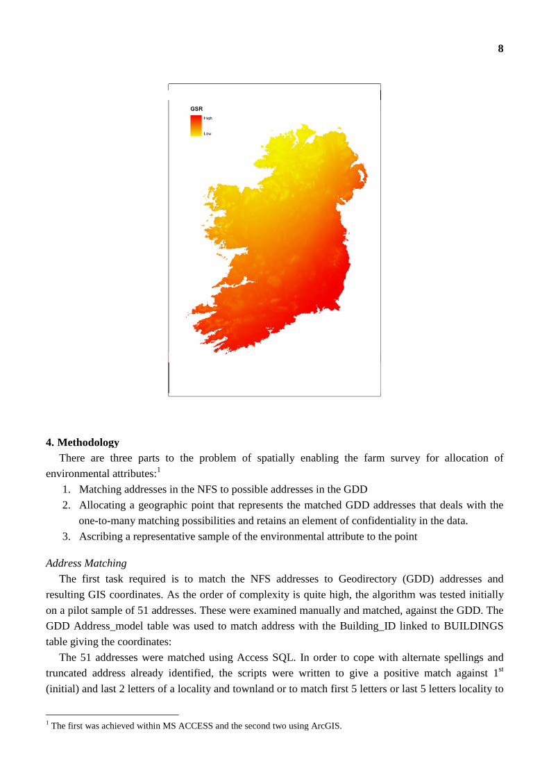
Spatial Environmental Data

For test purposes in this paper, we test the spatial representativity of weather data utilising historical

climate data generated by ICARUS, NUIM based on 30 (1960-1991) year means from Irish

Meteorological stations (Sweeny, Brereton et al. 2003). Models have been built at 1km grid cell scale

for the entire country. The data set used is the Mean Cumulative May-Oct Global Solar Radiation (40

year average) in effect the average for the 30 years in question of total amount of sunshine incident on

the ground over the summer months measured in kJ/m2 .The surface chosen was the accumulated

Global Solar Radiation map annual 40 year average, as shown in Figure 1.

Figure 1. Schematic showing geographic distribution of average accumulated summer (May to

October) Global Solar Radiation.

8

4. Methodology

There are three parts to the problem of spatially enabling the farm survey for allocation of

environmental attributes:1

1. Matching addresses in the NFS to possible addresses in the GDD

2. Allocating a geographic point that represents the matched GDD addresses that deals with the

one-to-many matching possibilities and retains an element of confidentiality in the data.

3. Ascribing a representative sample of the environmental attribute to the point

Address Matching

The first task required is to match the NFS addresses to Geodirectory (GDD) addresses and

resulting GIS coordinates. As the order of complexity is quite high, the algorithm was tested initially

on a pilot sample of 51 addresses. These were examined manually and matched, against the GDD. The

GDD Address_model table was used to match address with the Building_ID linked to BUILDINGS

table giving the coordinates:

The 51 addresses were matched using Access SQL. In order to cope with alternate spellings and

truncated address already identified, the scripts were written to give a positive match against 1st

(initial) and last 2 letters of a locality and townland or to match first 5 letters or last 5 letters locality to

1 The first was achieved within MS ACCESS and the second two using ArcGIS.

9

townland – matching always against county. The number five was used to allow bally* names to be

identified and *stown name to be identified (town is possessive in an Irish placename context and thus

is often preceded by ‘s’ e.g. Abbotstown).

This resulted in the automatic matching of 44 of the 51 NFS records – 3 more records could be

manually matched (the names were very different but recognisable) and the remaining 4 points are

manually matched against the most likely address(s).The NFS records were matched to GDD clusters

of addresses ranging from 1 to 45 houses.

After this pilot, we proceeded to the geo-enabling of the whole of the 2007 NFS address database.

The full list supplied contained 1350 records. Detailed examination of this list revealed a number of

data capture issues, such as different formats for the county name: Dublin or Co Dublin or Co. Dublin.

Also addresses were filled left to right so that AD3 was not always the county, sometimes it was blank

and there were also blank spaces at the end of entries (which, SQL unless instructed through the ‘ltrim’

‘rtrim’, commands recognises as characters). These issues and others could have been dealt with in

SQL but it was decided to do a preliminary clean of the input addresses in excel. Rules were refined

and added to. A common source of confusion was the swapping of address elements:

[Teagasc, Kinsealy, Malahide, Dublin] To =Teagasc, Malahide, Kinsealy, Dublin]

and other combinations. Thus the rules had to be expanded to include these permutations. An extra

set of rules that matched against the first two letters of the first three address elements was also

introduced.

A detailed examination of a subset of the unmatched set showed that the range of sources of error

were great and that to incorporate as SQL rules and run on the entire database would take longer than

manual checking.

Examples of the sort of errors are:

Teagasc, Malahyde, Kinsaley, Dublin

Resaecrh centre, Teagasc, kinsealy , malahgide, Dublin

Teagasc, Kinsealy , Swords, Dublin

Teagasc, Kinsealy, Malahide, Meath

The misallocation to County is common, either in the GDD, where the county is sometimes listed as

the county of the nearest post town, even if the townland is over the border. Also in the NFS it is not

uncommon in border areas for a townland to be identified as being in a different county.

Therefore the remaining names were checked and matched manually. Even with manual matching

85 addressed could not be identified with any confidence and have not been included in subsequent

analysis. A detailed examination of a subset of the unmatched set showed that the range of sources of

error were great and that to incorporate as SQL rules and run on the entire database would take longer

than manual checking.

Geo-locating

In order to link to environmental data, we need to go from an address to a location. As the majority

of NFS addresses match to multiple building points we have to decide how to allocate one point to the

10

NFS address with the assumption that in a one-to-many match one of the houses is the actual farm

house.

Because of the inherent precision in the environmental datasets, there is no need for precision

greater than 100m. For example, the digital soil map has a 75m limit to precision, the Teagasc

Indicative habitat map has a minimum mapping unit of 1ha (a nominal precision limit of 100m) and

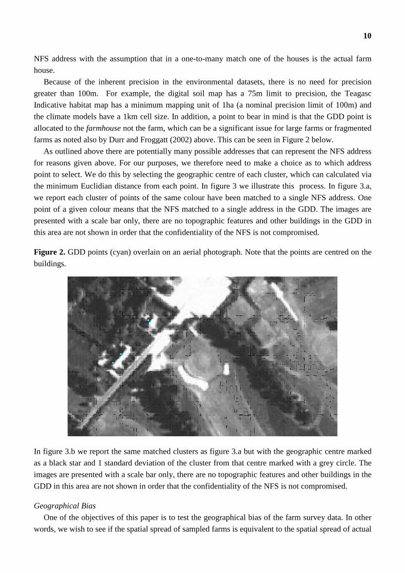
the climate models have a 1km cell size. In addition, a point to bear in mind is that the GDD point is

allocated to the farmhouse not the farm, which can be a significant issue for large farms or fragmented

farms as noted also by Durr and Froggatt (2002) above. This can be seen in Figure 2 below.

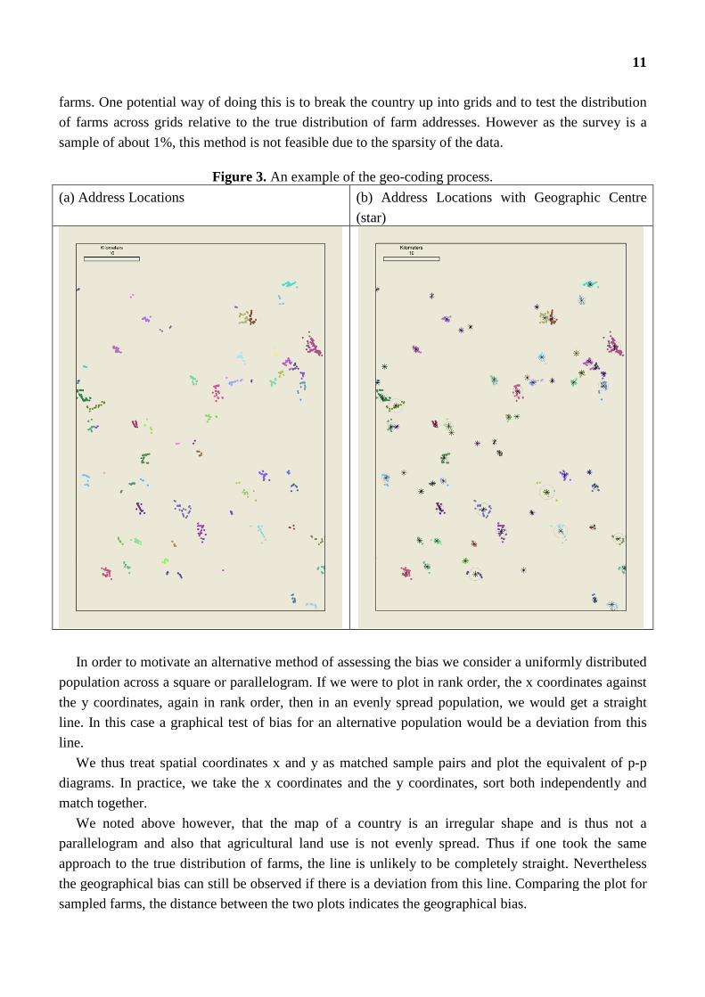
As outlined above there are potentially many possible addresses that can represent the NFS address

for reasons given above. For our purposes, we therefore need to make a choice as to which address

point to select. We do this by selecting the geographic centre of each cluster, which can calculated via

the minimum Euclidian distance from each point. In figure 3 we illustrate this process. In figure 3.a,

we report each cluster of points of the same colour have been matched to a single NFS address. One

point of a given colour means that the NFS matched to a single address in the GDD. The images are

presented with a scale bar only, there are no topographic features and other buildings in the GDD in

this area are not shown in order that the confidentiality of the NFS is not compromised.

Figure 2. GDD points (cyan) overlain on an aerial photograph. Note that the points are centred on the

buildings.

In figure 3.b we report the same matched clusters as figure 3.a but with the geographic centre marked

as a black star and 1 standard deviation of the cluster from that centre marked with a grey circle. The

images are presented with a scale bar only, there are no topographic features and other buildings in the

GDD in this area are not shown in order that the confidentiality of the NFS is not compromised.

Geographical Bias

One of the objectives of this paper is to test the geographical bias of the farm survey data. In other

words, we wish to see if the spatial spread of sampled farms is equivalent to the spatial spread of actual

11

farms. One potential way of doing this is to break the country up into grids and to test the distribution

of farms across grids relative to the true distribution of farm addresses. However as the survey is a

sample of about 1%, this method is not feasible due to the sparsity of the data.

Figure 3. An example of the geo-coding process.

(a) Address Locations (b) Address Locations with Geographic Centre

(star)

In order to motivate an alternative method of assessing the bias we consider a uniformly distributed

population across a square or parallelogram. If we were to plot in rank order, the x coordinates against

the y coordinates, again in rank order, then in an evenly spread population, we would get a straight

line. In this case a graphical test of bias for an alternative population would be a deviation from this

line.

We thus treat spatial coordinates x and y as matched sample pairs and plot the equivalent of p-p

diagrams. In practice, we take the x coordinates and the y coordinates, sort both independently and

match together.

We noted above however, that the map of a country is an irregular shape and is thus not a

parallelogram and also that agricultural land use is not evenly spread. Thus if one took the same

approach to the true distribution of farms, the line is unlikely to be completely straight. Nevertheless

the geographical bias can still be observed if there is a deviation from this line. Comparing the plot for

sampled farms, the distance between the two plots indicates the geographical bias.

12

An advantage of this method is that it can be used to compare distributions with different

underlying sizes. So for example there are about 120000 farms in the population, but only 1350 in our

sample. Nevertheless, the x and y coordinates can be plotted and compared against each other. At

present we have not developed a method to test the statistical properties of this comparison and so are

not in a position to test the statistical significance of the difference.

5. Results

The degree of error within the matching algorithm is within reasonable bounds and thus can be used

for our purpose. In this section we test the spatial-environmental representativity. To do this the spatial

pattern of geo-referenced NFS points are compared against national geographic and environmental

datasets.

Assessment of Geo-referencing

Utilising the algorithm described in section 4, we extend the pilot analysis, running the rules

sequentially; matching so combinations of 1350 addresses to a database of over 1.5 million. The

analysis took many hours and the result was about 1000 positive matches. These positive matches

sometimes included false positives but these are easy to eliminate by hand.

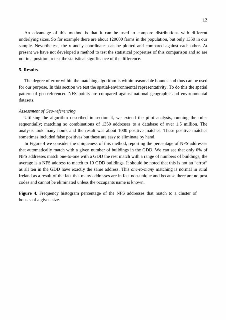
In Figure 4 we consider the uniqueness of this method, reporting the percentage of NFS addresses

that automatically match with a given number of buildings in the GDD. We can see that only 6% of

NFS addresses match one-to-one with a GDD the rest match with a range of numbers of buildings, the

average is a NFS address to match to 10 GDD buildings. It should be noted that this is not an “error”

as all ten in the GDD have exactly the same address. This one-to-many matching is normal in rural

Ireland as a result of the fact that many addresses are in fact non-unique and because there are no post

codes and cannot be eliminated unless the occupants name is known.

Figure 4. Frequency histogram percentage of the NFS addresses that match to a cluster of

houses of a given size.

13

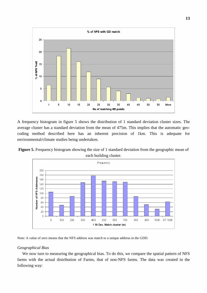
A frequency histogram in figure 5 shows the distribution of 1 standard deviation cluster sizes. The

average cluster has a standard deviation from the mean of 475m. This implies that the automatic geo-

coding method described here has an inherent precision of 1km. This is adequate for

environmental/climate studies being undertaken.

Figure 5. Frequency histogram showing the size of 1 standard deviation from the geographic mean of

each building cluster.

Note: A value of zero means that the NFS address was match to a unique address in the GDD.

Geographical Bias

We now turn to measuring the geographical bias. To do this, we compare the spatial pattern of NFS

farms with the actual distribution of Farms, that of non-NFS farms. The data was created in the

following way:

14

A national geographic distribution was established by randomly selecting 1000 points across

the Republic of Ireland (This is the NATional dataset).

This is also done for the other two data sets (the NFS points and the NON-nfs farming control

set).

Address points for non NFS farms was created by taking data from the CSO Census of

Agriculture 2000 at the district level, showing number of farmers, and average size of farm

have been used in testing the spatial characteristics of the NFS. (CSO, 2002). Centroids for all

Districts were calculated. All the districts with NFS points within them (~900) were eliminated

and so too were all the districts that, according to the CSO Census of Agriculture 2000, had no

farmers. This left ~1900 points (the district centroids) to act as dummy farms – the non-nfs set.

This sample set is geographically weighted but is not weighted to population of farmers.

An examination of possible geographic bias (bias used in a purely statistical sense) in Figure 6

indicates differences between the NFS set, the non nfs and a national set. Again because of

confidentially issues points on a map cannot be shown.

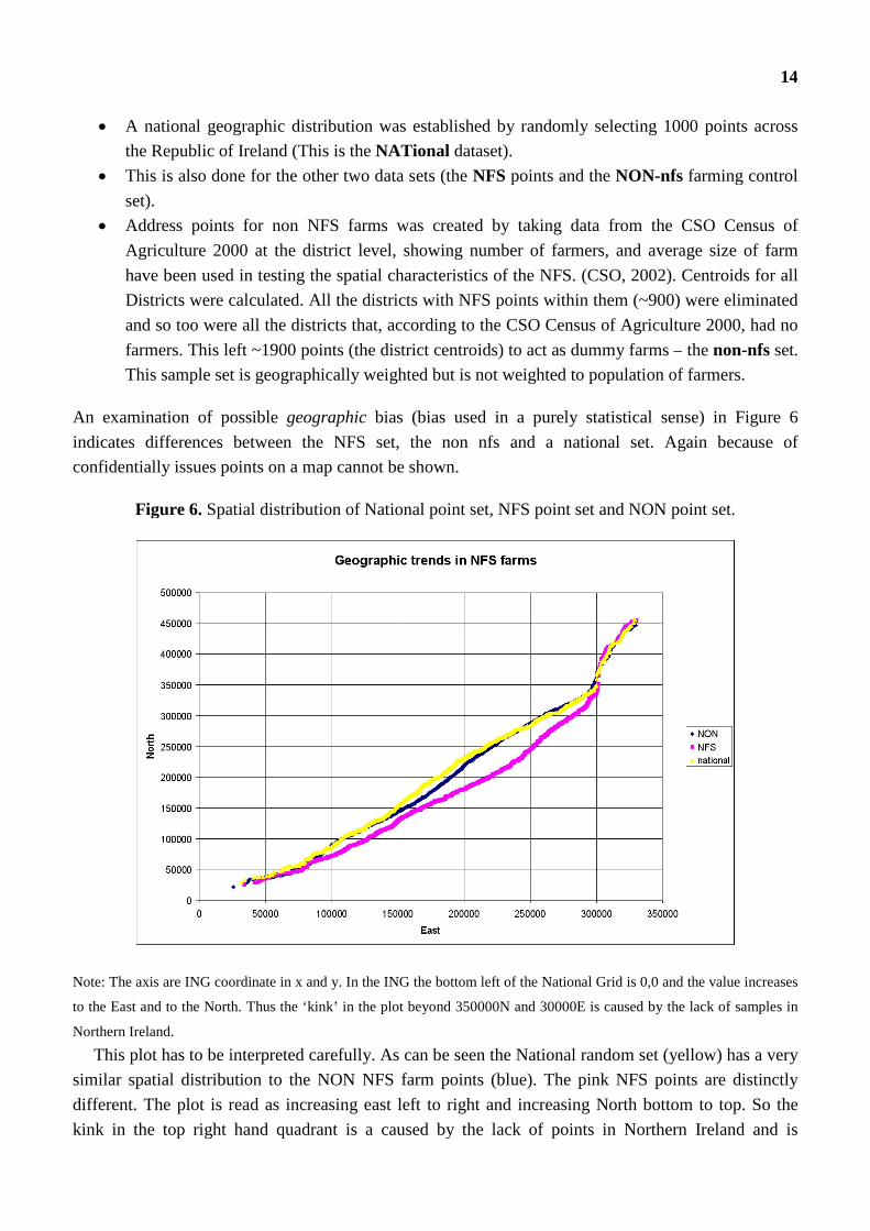
Figure 6. Spatial distribution of National point set, NFS point set and NON point set.

Note: The axis are ING coordinate in x and y. In the ING the bottom left of the National Grid is 0,0 and the value increases

to the East and to the North. Thus the ‘kink’ in the plot beyond 350000N and 30000E is caused by the lack of samples in

Northern Ireland.

This plot has to be interpreted carefully. As can be seen the National random set (yellow) has a very

similar spatial distribution to the NON NFS farm points (blue). The pink NFS points are distinctly

different. The plot is read as increasing east left to right and increasing North bottom to top. So the

kink in the top right hand quadrant is a caused by the lack of points in Northern Ireland and is

15

interpreted as above 350000N the points sampled are tending westward (Donegal). This should help in

interpreting the NFS data points. We can see, as the pink bulges below the national trend, that the

GNFS points trend both more easterly and southerly than the national and non-nfs sets.

In order to test the spatial-environmental representativity of the survey, we link our data points to

from the NFS-GDD match to environmental data. A test on using the NFS points to extract climate

information was also carried out. Climate surfaces as outlined above were used. We take from an

interpolated surface based on climate station trend data against elevation data. For each NFS the value

for the coincident 1 km cell was attributed to the NFS point as the levels of precision are the same. The

actual values are unimportant in this case we are interested in the trend of high levels of GSR in the SE

lower in the NW Figure 7 shows the distribution of values of the annual average accumulated summer

GSR for the three test sets, national, NON-NFS and NFS. In this case the national set is the values for

all the grid cells in the ROI map ( every 4th value, 5240 in total).

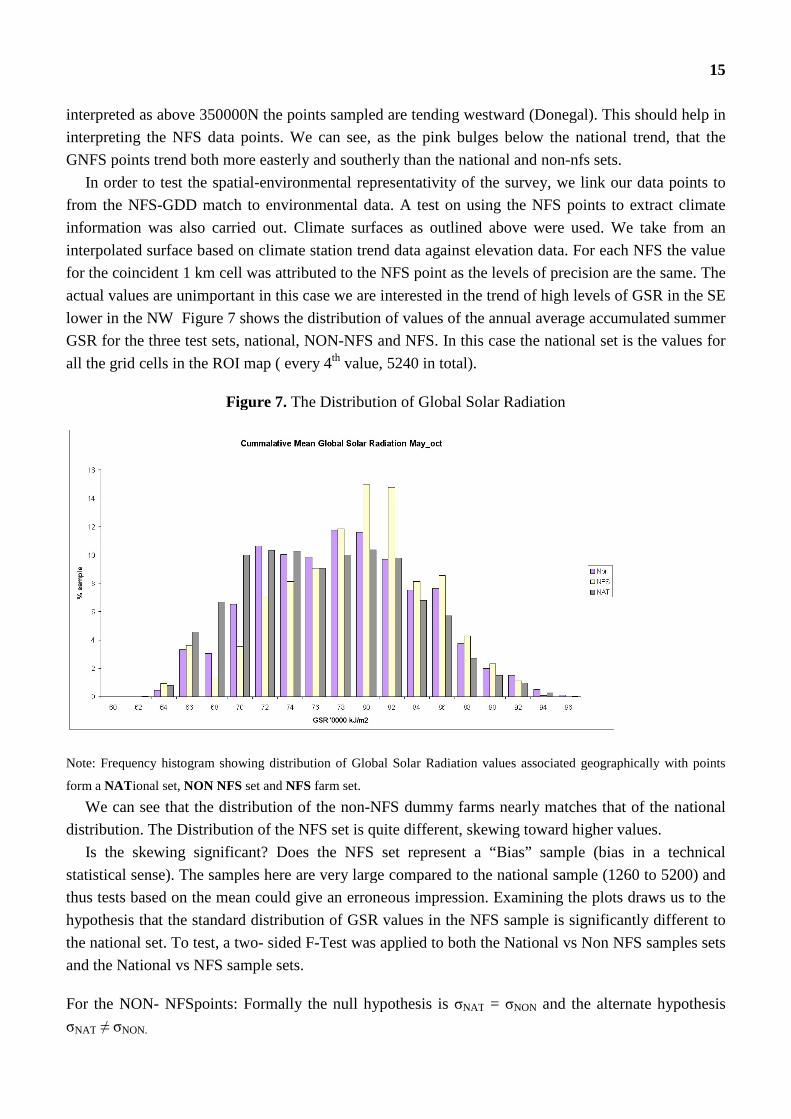
Figure 7. The Distribution of Global Solar Radiation

Note: Frequency histogram showing distribution of Global Solar Radiation values associated geographically with points

form a NATional set, NON NFS set and NFS farm set.

We can see that the distribution of the non-NFS dummy farms nearly matches that of the national

distribution. The Distribution of the NFS set is quite different, skewing toward higher values.

Is the skewing significant? Does the NFS set represent a “Bias” sample (bias in a technical

statistical sense). The samples here are very large compared to the national sample (1260 to 5200) and

thus tests based on the mean could give an erroneous impression. Examining the plots draws us to the

hypothesis that the standard distribution of GSR values in the NFS sample is significantly different to

the national set. To test, a two- sided F-Test was applied to both the National vs Non NFS samples sets

and the National vs NFS sample sets.

For the NON- NFSpoints: Formally the null hypothesis is σNAT = σNON and the alternate hypothesis

σNAT ≠ σNON.

16

Table 1. Summary two sided z-test for National/NON-NFS sets

nat non

Mean 75.74340295 77.08326

Variance 41.21613302 39.67419

Observations 5246 1898

Df 5245 1897

F 1.038865058

P(F<=f) one-tail 0.318

F Critical one-tail 1.077814282

The F value (1.038) is less than the critical f value (1.077 at 95% confidence limit) therefore the null

hypothesis is not rejected and we can say the standard deviation of both is the same. Thus the NON-

NFS sample set is a reliable sample of the national climate data examined.

For the NFS points: Formally the null hypothesis is σNAT = σNFS and the alternate hypothesis

σNAT ≠ σNFS

Table 2. Summary two sided z-test for National/NFS sets

nat Nfs

Mean 75.7434 78.03912656

Variance 41.21613 35.11558417

Observations 5246 1156

Df 5245 1155

F 1.173728

P(F<=f) one-tail 0.000638

F Critical one-tail 1.095755

In this case the F value (1.173) is greater than the critical value (1.09 at 95% confidence) therefore the

Null hypothesis is rejected in favour of the alternate, that the standard deviation of the NFS sample is

significantly different to national sample.

We also test difference of farm characteristics between the GNFS and the non-NFS datasets, by

looking at farm characteristics of the Districts with NFS points and compare to those without. Average

farm size is covariant with many other economic variables and thus was selected as a test variable.

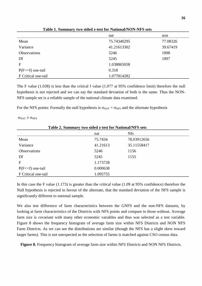
Figure 8 shows the frequency histogram of average farm size within NFS Districts and NON NFS

Farm Districts. As we can see the distributions are similar (though the NFS has a slight skew toward

larger farms). This is not unexpected as the selection of farms is matched against CSO census data.

Figure 8. Frequency histogram of average farm size within NFS Districts and NON NFS Districts.

17

6. Discussion

The NFS dataset shows a geographic bias toward south east of the country. This is not unexpected as

the NFS is designed to give a representative national sample of the main farm enterprises. In Ireland

these enterprises are themselves geographically biased and localised. Crudely; tillage is in the South

and East of Ireland, dairy in the south and beef nationally. So it would be expected that any sampling

system stratified on these sectors would be spatially biased to the South East. Climatic and

environmental data are also geographically weighted again with a SE/NW axis. Naturally the two facts

are complimentary, in that the enterprises occur in environmentally suitable locations.

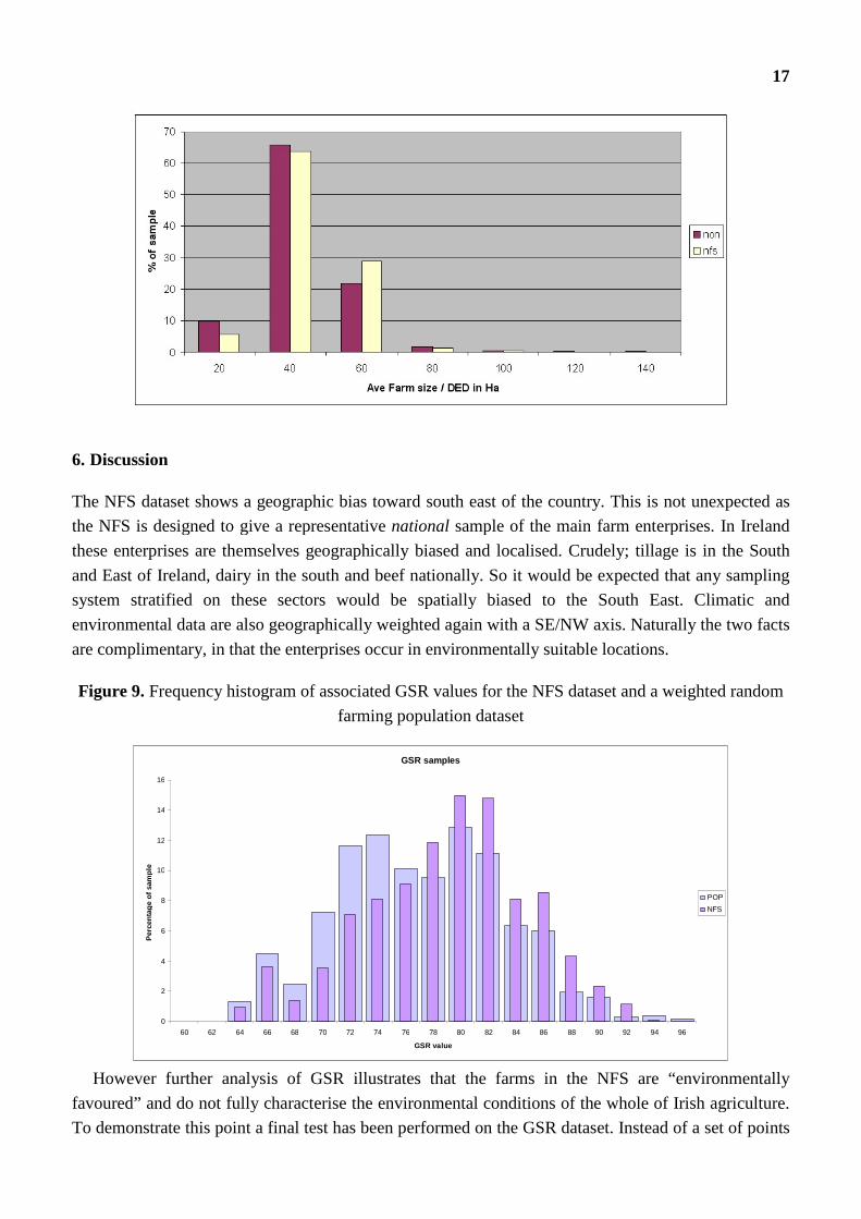
Figure 9. Frequency histogram of associated GSR values for the NFS dataset and a weighted random

farming population dataset

GSR samples

0

2

4

6

8

10

12

14

16

60 62 64 66 68 70 72 74 76 78 80 82 84 86 88 90 92 94 96

GSR value

Perc

en

tag

eo

fsam

ple

POP

NFS

However further analysis of GSR illustrates that the farms in the NFS are “environmentally

favoured” and do not fully characterise the environmental conditions of the whole of Irish agriculture.

To demonstrate this point a final test has been performed on the GSR dataset. Instead of a set of points

18

randomly distributed we have created a random sample of points (n=979), weighted for farming

population density from the CSO figures (the more farms in an area the higher the chance of a random

point occurring). A percentage frequency histogram of the GSR measurement for each of the

population weighted (pop) points is plotted along with the equivalent NFS set we have already seen.

Figure 9 shows the differences the two samples and an analysis of the two samples shows significant

variance between means:

So we can say that the geographic bias of the NFS sample means that the NFS points do not fully

represent some environmental/climatic geographies in Ireland as they impact on the farming

population as a whole. So for example if we wish to use the NFS data to look at climate change

impacts or adaptation strategies, especially amongst beef producers in the West we may run into

difficulty as the SE bias means that some environmental combinations (soil/weather) will be under

sampled or not sampled at all.

7. Conclusion

In this paper we developed an algorithm to geo-reference farm households in the Irish sample of the

Farm Accountancy Data Network (FADN). Testing for geographical bias, we note a slight difference

between the sample and the underlying distribution.

The National Farm Survey, as part of FADN, is designed to accurately represent farm systems. The

geo-referencing of farm survey data enables future analyses of the distribution between farm output

and cost data and environmental attributes. However, as we have shown here that, in Ireland’s case, it

does not represent farm geography fully, the data may limit some analyses where particular

combinations of environmental variables and farm variables are missing due to the nature of the

sample.

As the European FADN system moves toward introducing a geospatial element to its reporting it

may be necessary to adapt the current sampling strategies to ensure that the sample chosen equally

represents geography (both European and national) as well systems performance. It cannot be assumed

that a 1% sample of European farms systems will represent the full environmental geography of

European agriculture.

References

Allen, R., R. Bosecker, et al. POLICY ISSUES ASSOCIATED WITH THE UTILIZATION OF

GEOGRAPHIC

Charlier, Hubert (2009) The EU Farm Structure Surveys from 2010 Onwards. Eurostat Mimeo

Connolly, L., A.Kinsella, et al. (2008). National Farm Survey 2007, Teagasc.

Corbett, John D. (1996). The changing face of agroecosystem characterization: Models and Spatial

Data, the Basis for Robust Agroecosytem Characterization., In: Proceedings of the 3rd International

Conference on Integrating GIS and Environmental Modelling. Santa Fe, NM

http://www.ncgia.ucsb.edu/conf/SANTA_FE_CDROM/sf_papers/corbett_john/corbett.html

19

Coulter, B. S., E. McDonald, et al. (1999). VISUAL ENVIRONMENTAL DATA ON SOILS AND

LANDUSE END OF PROJECT REPORT ARMIS 4496. Rural Environmental Series, TEAGASC: 46.

Durr PA, Froggatt AE.(2002). How best to geo-reference farms? A case study from Cornwall,

England. Prev Vet Med. 29;56(1):51-62.

Fahey, D. and F. Finch (2008). GeoDirectory Technical Guide, An Post/OSI.

Fais, A., P. Nino, et al. (2005). MICROECONOMIC AND GEO-PHYSICAL DATA INTEGRATION

FOR AGRI-ENVIRONMENTAL ANALYSIS, GEOREFERENCING FADN DATA: A CASE

STUDY IN ITALY. XIth seminar of the European Association of Agricultural Economists.

Copenhagen, Denmark, EAAE.

GPO 2001, Ordnance Survey Ireland Act, Government Publication Office

Hassan, R. M.; Corbett, J. D.; Njoroge, K. (1998) Combining geo-referenced survey data with

agroclimatic attributes to characterize maize production systems in Kenya. In Hassan, R. M. (Ed.)

Maize technology development and transfer: a GIS application for research planning in Kenya. pp. 43-

68.

Holloway, G., D. Lacombe, et al. (2006). Spatial Econometric Issues for Bio-Economic and Land-Use

Modeling. International Association of Agricultural Economists Conference,. Gold Coast, Australia,.

INFORMATION SYSTEMS (GIS) IN THE U.S. NATIONAL AGRICULTURAL STATISTICS

SERVICE (NASS), US National Agricultural Statistics Service.

Kokic, Philip, Kenton Lawson, Alistair Davidson, Lisa Elliston, Collecting Geo-Referenced Data in

Farm Surveys, Papers presented at the ICES-III, June 18-21, 2007, Montreal, Quebec, Canada

Sweeney, J., T. Brereton, et al. (2003). Climate Change: Scebario & Impacts for Ireland, EPA.

VanWey, L. K., R. R. Rindfuss, et al. (2005). "Confidentiality and spatially explicit data: Concerns

and challenges." Proc Natl Acad Sci U S A 102(43): 15337–15342.