Chapter 1: Assessment of the Walleye Pollock Stock in the Gulf of Alaska

Martin Dorn1, Kerim Aydin1, Steven Barbeaux1, Michael Guttormsen1,

Kally Spalinger2, and Wayne Palsson1

1 National Marine Fisheries Service, Alaska Fisheries Science Center, Seattle, WA 2 Alaska Department of Fish and Game, Division of Commercial Fisheries, Kodiak, AK

Executive Summary

Summary of Changes in Assessment Inputs

Changes in input data 1. Fishery: 2010 total catch and catch at age. 2. NMFS bottom trawl survey: 2011 biomass and length composition. 3. ADF&G crab/groundfish trawl survey: 2011 biomass and length composition. Changes in assessment methodology The age-structured assessment model developed using ADModel Builder (a C++ software language extension and automatic differentiation library) and used for assessments in 1999-2010 was used again for this year’s assessment. Summary of Results

The model projection of spawning biomass in 2012 is 227,723 t, which is 33.6% of unfished spawning biomass (based on average post-1977 recruitment) and below B40% (271,000 t), thereby placing Gulf of Alaska pollock in sub-tier “b” of Tier 3. New NFMS bottom trawl and ADF&G crab/groundfish surveys were conducted in 2011. The 2011 NMFS bottom trawl survey biomass estimate was very close to the 2009 estimate (<1% increase). The ADF&G crab/groundfish survey biomass estimate declined 19% from the 2010 biomass estimate, but is 32% above the mean for 2006-2008. Recent estimates from both surveys are fit adequately by the model, and there are no large residuals to the fit to recent age data. No acoustic surveys were conducted in winter of 2011, increasing the uncertainty of the assessment model relative to previous years. The estimated abundance of mature fish in 2012 is projected to be 11% higher than in 2011, and is projected to increase gradually over the next five years. The author’s 2012 ABC recommendation for pollock in the Gulf of Alaska west of 140° W lon. (W/C/WYK) is 108,440 t, an increase of 22% from the 2011 ABC. This recommendation is based on a more conservative alternative to the maximum permissible FABC introduced in the 2001 SAFE. The OFL in 2012 is 143,716 t. In 2013, the recommended ABC and OFL are 117,325 t and 155,402 t, respectively. For pollock in southeast Alaska (East Yakutat and Southeastern areas), the ABC recommendations for 2012 and 2013, presented in Appendix A, are 10,774 t and the OFL recommendation for 2012 and 2013 is 14,366 t. These recommendations are based on the estimated biomass in the southeast Alaska from the 2011 NMFS bottom trawl survey.

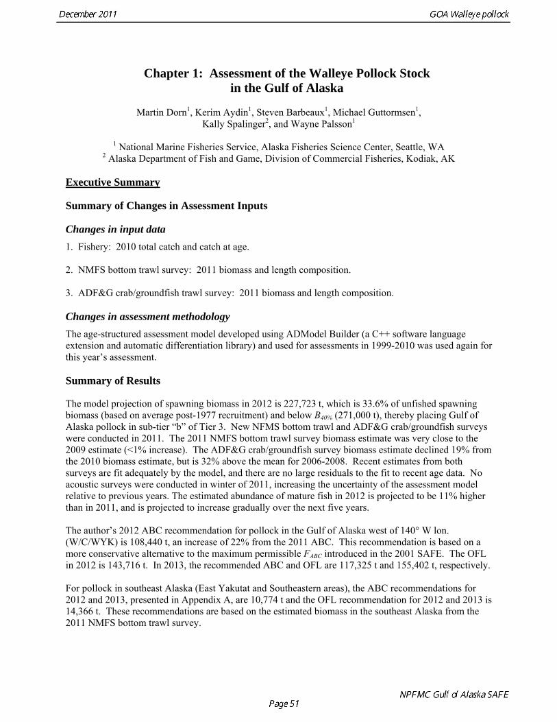
Status Summary Table

Last year This year Quantity/Status 2011 2012 2012 2013M (natural mortality) 0.3 0.3 0.3 0.3Specified/recommended Tier 3b 3b 3b 3bProjected biomass (ages 3+) 893,700 988,580 863,840 926,890Female spawning biomass (t) Projected 198,767 227,345 227,723 232,632 B100% 690,000 678,000 B40% 276,000 271,000 B35% 242,000 237,000 FOFL 0.16 0.18 0.19 0.19maxFABC 0.14 0.16 0.17 0.17Specified/recommended FABC 0.12 0.14 0.14 0.15Specified/recommended OFL (t) 118,030 151,030 143,720 155,400Specified/recommended Max. Permissible ABC (t) 102,940 127,990 125,560 135,790Specified/recommended ABC (t) 88,620 114,054 108,440 117,330Is the stock being subjected to overfishing? No No Is the stock currently overfished? No No Is the stock approaching a condition of being overfished? No No Responses to Comments of the Scientific and Statistical Committee (SSC) The SSC did not make any comments specific to the Gulf of Alaska pollock assessment in its December 2010 minutes. A CIE review of the Gulf of Alaska pollock assessment is scheduled for 2012. We anticipate providing full a new assessment for initial review by the CIE panel, followed by plan team and SSC review. The SSC may wish to give guidance on priority issues that the CIE panel should address during its review. The CIE review will also give the assessment authors the opportunity to address earlier SSC comments on data weighting, survey catchability, and extending the age range of the model.

Introduction

Walleye pollock (Theragra chalcogramma) is a semi-pelagic schooling fish widely distributed in the North Pacific Ocean. Pollock in the Gulf of Alaska are managed as a single stock independently of pollock in the Bering Sea and Aleutian Islands. The separation of pollock in Alaskan waters into eastern Bering Sea and Gulf of Alaska stocks is supported by analysis of larval drift patterns from spawning locations (Bailey et al. 1997), genetic studies of allozyme frequencies (Grant and Utter 1980), mtDNA variability (Mulligan et al. 1992), and microsatellite allele variability (Bailey et al. 1997). The results of studies of stock structure in the Gulf of Alaska are equivocal. There is evidence from allozyme frequency and mtDNA that spawning populations in the northern part of the Gulf of Alaska (Prince William Sound and Middleton Island) may be genetically distinct from the Shelikof Strait spawning population (Olsen et al. 2002). However significant variation in allozyme frequency was found between Prince William Sound samples in 1997 and 1998, indicating a lack of stability in genetic structure for this spawning population. Olsen et al. (2002) suggest that interannual genetic variation may be due to variable reproductive success, adult philopatry, source-sink population structure, or utilization of the same spawning areas by genetically distinct stocks with different spawning timing. Peak spawning at the two major spawning areas in the Gulf of Alaska occurs at different times. In the Shumagin Island area, peak spawning apparently occurs between February 15- March 1, while in Shelikof Strait peak spawning occurs later, typically between March 15 and April 1. It is unclear whether the difference in timing is genetic, or a response to differing environmental conditions in the two areas. Fishery

The commercial fishery for walleye pollock in the Gulf of Alaska started as a foreign fishery in the early 1970s (Megrey 1989). Catches increased rapidly during the late 1970s and early 1980s (Table 1.1). A large spawning aggregation was discovered in Shelikof Strait in 1981, and a fishery developed for which pollock roe was an important product. The domestic fishery for pollock developed rapidly in the Gulf of Alaska with only a short period of joint venture operations in the mid-1980s. The fishery was fully domestic by 1988. The fishery for pollock in the Gulf of Alaska is entirely shore-based with approximately 90% of the catch taken with pelagic trawls. During winter, fishing effort targets pre-spawning aggregations in Shelikof Strait and near the Shumagin Islands (Fig. 1.1). Fishing in summer is less predictable, but typically occurs on the east side of Kodiak Island and along the Alaska Peninsula. Incidental catch in the Gulf of Alaska directed pollock fishery is low. For tows classified as pollock targets in the Gulf of Alaska between 2006 and 2010, on average about 93% of the catch by weight of FMP species consisted of pollock (Table 1.2). Nominal pollock targets are defined by the dominance of pollock in the catch, and may include tows where other species were targeted, but where pollock were caught instead. The most common managed species in the incidental catch are arrowtooth flounder, Pacific cod, flathead sole, Pacific ocean perch, miscellaneous flatfish, and the shortraker/rougheye rockfish complex. The most common non-target species are squid, eulachon, various shark species (e.g., Pacific sleeper sharks, spiny dogfish, salmon shark), jellyfish, and grenadiers. Bycatch estimates for prohibited species over the period 2006-2010 are given in Table 1.3. Bycatch of Chinook salmon is the most consequential prohibited species caught as bycatch in the pollock fishery. The peak in Chinook salmon bycatch in 2010 led the Council to adopt management measures to reduce Chinook salmon bycatch. Kodiak is the major port for pollock in the Gulf of Alaska, with 65% of the 2006-2010 landings. In the western Gulf of Alaska, Sand Point, Dutch Harbor, King Cove, and Akutan are important ports, sharing

35% of 2006-2010 landings. Secondary ports, including Alitak Bay, Cordova, Homer, Juneau, Ketchikan, Ninilchik, Seward, and Sitka account for less than 1% of the 2006-2010 landings. Since 1992, the Gulf of Alaska pollock Total Allowable Catch (TAC) has been apportioned spatially and temporally to reduce potential impacts on Steller sea lions. The details of the apportionment scheme have evolved over time, but the general objective is to allocate the TAC to management areas based on the distribution of surveyed biomass, and to establish three or four seasons between mid-January and autumn during which some fraction of the TAC can be taken. The Steller Sea Lion Protection Measures implemented in 2001 established four seasons in the Central and Western GOA beginning January 20, March 10, August 25, and October 1, with 25% of the total TAC allocated to each season. Allocations to management areas 610, 620 and 630 are based on the seasonal biomass distribution as estimated by groundfish surveys. In addition, a new harvest control rule was implemented that requires suspension of directed pollock fishing when spawning biomass declines below 20% of the reference unfished level. Data Used in the Assessment

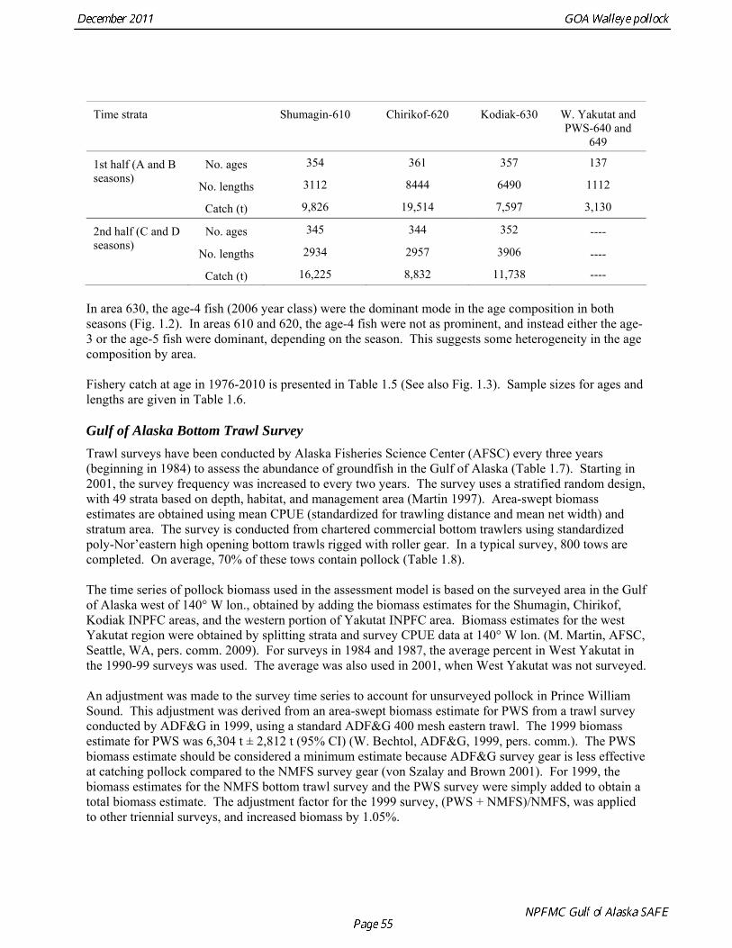
The data used in the assessment model consist of estimates of annual catch in tons, fishery age composition, NMFS summer bottom trawl survey estimates of biomass and age composition, acoustic survey estimates of biomass and age composition in Shelikof Strait, egg production estimates of spawning biomass in Shelikof Strait, ADF&G bottom trawl survey estimates of biomass and length and age composition, and historical estimates of biomass and length and age composition from surveys conducted prior to 1984 using a 400-mesh eastern trawl. Binned length composition data are used in the model only when age composition estimates are unavailable, such as the fishery in the early part of the modeled time period and the most recent survey. The FOCI year class prediction is used qualitatively along with other information to evaluate the likely strength of incoming year classes. Total Catch Estimated catch was derived by the NMFS Regional Office from shoreside electronic logbooks and observer estimates of at-sea discards (Table 1.4). Catches include the state-managed pollock fishery in Prince William Sound (PWS). Non-commercial catches and pollock bycatch in the halibut fishery are reported in Appendix D. Since 1996 the pollock Guideline Harvest Level (GHL) for the PWS fishery has been deducted from the Acceptable Biological Catch (ABC) by the NPFMC Gulf of Alaska Plan Team for management purposes. Fishery Age Composition Estimates of fishery age composition were derived from at-sea and port sampling of the pollock catch for length and ageing structures (otoliths). Pollock otoliths collected during the 2010 fishery were aged using the revised criteria described in Hollowed et al. (1995), which involved refinements in the criteria to define edge type. Catch age composition was estimated using methods described by Kimura and Chikuni (1989). Age samples were used to construct age-length keys by sex and stratum. These keys were applied to sex and stratum specific length frequency data to estimate age composition, which were then weighted by the catch in numbers in each stratum to obtain an overall age composition. Age and length samples from the 2010 fishery were stratified by half year and statistical area as follows:

Time strata Shumagin-610 Chirikof-620 Kodiak-630 W. Yakutat and

PWS-640 and 649

No. ages 354 361 357 137 1st half (A and B seasons)

No. lengths 3112 8444 6490 1112

Catch (t) 9,826 19,514 7,597 3,130

No. ages 345 344 352 ---- 2nd half (C and D seasons)

No. lengths 2934 2957 3906 ----

Catch (t) 16,225 8,832 11,738 ---- In area 630, the age-4 fish (2006 year class) were the dominant mode in the age composition in both seasons (Fig. 1.2). In areas 610 and 620, the age-4 fish were not as prominent, and instead either the age-3 or the age-5 fish were dominant, depending on the season. This suggests some heterogeneity in the age composition by area. Fishery catch at age in 1976-2010 is presented in Table 1.5 (See also Fig. 1.3). Sample sizes for ages and lengths are given in Table 1.6. Gulf of Alaska Bottom Trawl Survey Trawl surveys have been conducted by Alaska Fisheries Science Center (AFSC) every three years (beginning in 1984) to assess the abundance of groundfish in the Gulf of Alaska (Table 1.7). Starting in 2001, the survey frequency was increased to every two years. The survey uses a stratified random design, with 49 strata based on depth, habitat, and management area (Martin 1997). Area-swept biomass estimates are obtained using mean CPUE (standardized for trawling distance and mean net width) and stratum area. The survey is conducted from chartered commercial bottom trawlers using standardized poly-Nor’eastern high opening bottom trawls rigged with roller gear. In a typical survey, 800 tows are completed. On average, 70% of these tows contain pollock (Table 1.8). The time series of pollock biomass used in the assessment model is based on the surveyed area in the Gulf of Alaska west of 140° W lon., obtained by adding the biomass estimates for the Shumagin, Chirikof, Kodiak INPFC areas, and the western portion of Yakutat INPFC area. Biomass estimates for the west Yakutat region were obtained by splitting strata and survey CPUE data at 140° W lon. (M. Martin, AFSC, Seattle, WA, pers. comm. 2009). For surveys in 1984 and 1987, the average percent in West Yakutat in the 1990-99 surveys was used. The average was also used in 2001, when West Yakutat was not surveyed. An adjustment was made to the survey time series to account for unsurveyed pollock in Prince William Sound. This adjustment was derived from an area-swept biomass estimate for PWS from a trawl survey conducted by ADF&G in 1999, using a standard ADF&G 400 mesh eastern trawl. The 1999 biomass estimate for PWS was 6,304 t ± 2,812 t (95% CI) (W. Bechtol, ADF&G, 1999, pers. comm.). The PWS biomass estimate should be considered a minimum estimate because ADF&G survey gear is less effective at catching pollock compared to the NMFS survey gear (von Szalay and Brown 2001). For 1999, the biomass estimates for the NMFS bottom trawl survey and the PWS survey were simply added to obtain a total biomass estimate. The adjustment factor for the 1999 survey, (PWS + NMFS)/NMFS, was applied to other triennial surveys, and increased biomass by 1.05%.

The Alaska Fisheries Science Center’s (AFSC) Resource Assessment and Conservation Engineering (RACE) Division conducted the twelfth comprehensive bottom trawl survey since 1984 during the summer of 2011. The spatial distribution of pollock is consistent with previous surveys (Fig. 1.4). Areas with higher CPUE included the east side of Kodiak Island, and nearshore along the Alaska Peninsula. The 2010 gulfwide biomass estimate of pollock was 708,092 t, which is very close to 2009 estimate (<1% increase). The biomass estimate for the portion of the Gulf of Alaska west of 140º W long. is 667,131 t. Bottom Trawl Age Composition Estimates of numbers at age from the bottom trawl survey were obtained from random otolith samples and length frequency samples (Table 1.9). Numbers at age were estimated by INPFC area (Shumagin, Chirikof, Kodiak, Yakutat and Southeastern) using a global age-length key and CPUE-weighted length frequency data by INPFC area. The combined Shumagin, Chirikof and Kodiak age composition was used in the assessment model. Ages are not yet available for the 2011 survey, and instead lengths were used in the assessment model. Length composition by statistical area showed a mode of age-1 fish in all areas that increased in size from the Shumagin area to the Southeast area, most likely due to seasonal growth during the course of the survey (Fig. 1.5). This pattern has been seen in previous bottom trawl surveys. Mean size generally decreased from west to east (ranging from 49 cm in the Shumagin area to 28 cm years in the Yakutat area). Shelikof Strait Acoustic Survey Acoustic surveys to assess the biomass of pollock in the Shelikof Strait area have been conducted annually since 1981 (except 1982 and 1999). Survey methods and results for 2010 are presented in a NMFS processed report (Guttormsen et. al. in review). Biomass estimates using the Simrad EK echosounder from 1992 onwards were re-estimated to take into account recently published work of eulachon acoustic target strength (Gauthier and Horne 2004). Previously, acoustic backscatter was attributed to eulachon based on the percent composition of eulachon in trawls, and it was assumed that eulachon had the same target strength as pollock. Since Gauthier and Horne (2004) determined that the target strength of eulachon was much lower than pollock, the acoustic backscatter could be attributed entirely to pollock even when eulachon were known to be present. In 2008, the noise-reduced R/V Oscar Dyson became the designated survey vessel for acoustic surveys in the Gulf of Alaska. In winter of 2007, a vessel comparison experiment was conducted between the R/V Miller Freeman (MF) and the R/V Oscar Dyson (OD), which obtained an OD/MF ratio of 1.132 in Shelikof Strait. The Shelikof Strait acoustic survey was not conducted in 2011 due to scheduled repairs to the R/V Oscar Dyson. This is the first interruption in the annual Shelikof Strait acoustic survey time series since 1999 (Fig. 1.6). Winter acoustic surveys in other regions of the Gulf of Alaska (Chirikof, Shumagin Islands, Sanak Gully) (Fig 1.7) were also canceled due to the scheduled repairs. Since the assessment model only includes age 2 and older pollock, the biomass of age-1 fish in the 1995, 2000, 2005, and 2008 surveys was subtracted from the total biomass for those years, reducing the biomass by 15%, 13%, 5% and 9% respectively (Table 1.7). In all other years, the biomass of age-1 fish was less than 2% of the total acoustic biomass estimate. Acoustic Survey Length Frequency Annual biomass distributions by length from the Shelikof Strait acoustic survey show the progression of strong year classes through the population (Fig. 1.8). Since age composition estimates are available for all surveys, size composition data were not used in the assessment model. Acoustic Trawl Survey Age Composition Estimates of numbers at age from the Shelikof Strait acoustic survey (Table 1.10) were obtained from

random otolith samples and length frequency samples. Otoliths collected during the 1994 - 2010 acoustic surveys were aged using the criteria described in Hollowed et al. (1995). Sample sizes for ages and lengths are given Table 1.11. Summer acoustic survey Scientists from AFSC conducted an acoustic survey on NOAA Ship Oscar Dyson in the Gulf of Alaska from June 12 to August 12, 2011 (Fig. 1.9). Although the objective of the survey was to cover the shelf and nearshore areas of Gulf of Alaska from the Islands of Four Mountains (170° long. W) to Yakutat Bay (140° long. W), equipment failure, crew injuries and ensuing staffing issues prevented this objective from being achieved. The survey extended approximately to the eastern end of Kodiak Island, and did not cover the area for the assessment model, and therefore was not considered for inclusion in the model. Using results from the 2011 NMFS bottom trawl survey for comparison, the biomass from strata covered (in full or in part) by the acoustic survey was approximately 85% of the total bottom trawl biomass for the assessment area. A preliminary estimate of the biomass for the acoustic survey is 454,023 t, which is 80% of bottom trawl estimate for this area. While there are a number of reasons not to rely too much on these comparisons, they are useful to establish that abundance estimates from the bottom trawl survey and acoustic survey are broadly similar in magnitude, and that the acoustic survey covered most but not all of the area where pollock are found in high abundance. The length composition for the acoustic survey in 2011 compared to bottom trawl suggests that larger fish were relatively more available to bottom trawl (Figure 1.10). The acoustic survey abundance estimate of pollock <22 cm (considered a reliable proxy for age-1 pollock) is 1.6 billion, more than three times the bottom trawl estimate, suggesting that the acoustic survey is more effective at sampling age-1 pollock. Age-1 pollock were found primarily in Shelikof Strait. If an estimate of this magnitude had occurred during the winter survey in Shelikof Strait, it would rank 5th out of 28 age-1 estimates (82nd quantile), suggesting that the 2010 year class is relatively strong. The summer estimate is likely be a conservative estimate in this comparison due to the high mortality rates experienced by juvenile pollock. Egg Production Estimates of Spawning Biomass Estimates of spawning biomass in Shelikof Strait based on egg production methods were included in the assessment model. A complete description of the estimation process is given in Picquelle and Megrey (1993). The estimates of spawning biomass in Shelikof Strait show a pattern similar to the acoustic survey (Table 1.7). The annual egg production spawning biomass estimate for 1981 is questionable because of sampling deficiencies during the egg surveys for that year (Kendall and Picquelle 1990). Coefficients of variation (CV) associated with these estimates were included in the assessment model. Egg production estimates were discontinued because the Shelikof Strait acoustic survey provided similar information. Alaska Department of Fish and Game Crab/Groundfish Trawl Survey The Alaska Department of Fish and Game (ADF&G) has conducted bottom trawl surveys of nearshore areas of the Gulf of Alaska since 1987. Although these surveys are designed to monitor population trends of Tanner crab and red king crab, walleye pollock and other fish are also sampled. Standardized survey methods using a 400-mesh eastern trawl were employed from 1987 to the present. The survey is designed to sample a fixed number of stations from mostly nearshore areas from Kodiak Island to Unimak Pass, and does not cover the entire shelf area. The average number of tows completed during the survey is 360. Details of the ADF&G trawl gear and sampling procedures are in Blackburn and Pengilly (1994).

The 2010 biomass estimate for pollock for the ADF&G crab/groundfish survey was 100,839 t, down 19% from the 2010 biomass estimate, but still an increase of approximately 32% from the mean during 2006-2008 (Table 1.7). ADF&G Survey Length Frequency Pollock length-frequencies for the ADF&G survey in 1989-2011 (excluding 1991 and 1995) typically show a mode at lengths greater than 45 cm (Fig. 1.11). The predominance of large fish in the ADF&G survey may result from the selectivity of the gear, or because of greater abundance of large pollock in the areas surveyed. Length composition in 2011 is similar to previous surveys, with a mean length of 53 cm. ADF&G Survey Age Composition Ages were determined by age readers in the AFSC age and growth unit from samples of pollock otoliths collected during the 2000, 2002, 2004, 2006, 2008, and 2010 ADF&G surveys (N = 559, 538, 591,588, 597, and 585). Comparison with fishery age composition shows that older fish (> age-8) are more common in the ADF&G crab/groundfish survey. This is consistent with the assessment model, which estimates a domed-shaped selectivity pattern for the fishery, but an asymptotic selectivity pattern for the ADF&G survey. Pre-1984 bottom trawl surveys Considerable survey work was carried out in the Gulf of Alaska prior to the start of the NMFS triennial bottom trawl surveys in 1984. Between 1961 and the mid-1980s, the most common bottom trawl used for surveying was the 400-mesh eastern trawl. This trawl (or minor variants thereof) was used by IPHC for juvenile halibut surveys in the 1960s, 1970s, and early 1980s, and by NMFS for groundfish surveys in the 1970s. Comparative work using the ADF&G 400-mesh eastern trawl and the NMFS poly-Nor’eastern trawl produced estimates of relative catchability (von Szalay and Brown 2001), making it possible to evaluate trends in pollock abundance from these earlier surveys in the pollock assessment. Von Szalay and Brown (2001) estimated a fishing power correction (FPC) for the ADF&G 400-mesh eastern trawl of 3.84 (SE = 1.26), indicating that 400-mesh eastern trawl CPUE for pollock would need to be multiplied by this factor to be comparable to the NMFS poly-Nor’eastern trawl. In most cases, earlier surveys in the Gulf of Alaska were not designed to be comprehensive, with the general strategy being to cover the Gulf of Alaska west of Cape Spencer over a period of years, or to survey a large area to obtain an index for group of groundfish, i.e., flatfish or rockfish. For example, Ronholt et al. (1978) combined surveys for several years to obtain gulfwide estimates of pollock biomass for 1973-6. There are several difficulties with such an approach, including the possibility of double-counting or missing a portion of the stock that happened to migrate between surveyed areas. An annual gulfwide index of pollock abundance was obtained using generalized linear models (GLM). Based on examination of historical survey trawl locations, four index sites were identified (one per INPFC area) that were surveyed relatively consistently during the period 1961-1983, and during the triennial survey time series (1984-99). The index sites were designed to include a range of bottom depths from nearshore to the continental slope. A generalized linear model (GLM) was fit to pollock CPUE data with year, site, depth strata (0-100 m, 100-200 m, 200-300 m, >300 m), and a site-depth interaction as factors. Both the pre-1984 400-mesh eastern trawl data and post-1984 triennial trawl survey data were used. For the earlier period, analysis was limited to sites where at least 20 trawls were made during the summer (May 1-Sept 15). Pollock CPUE data consist of observations with zero catch and positive values otherwise, so a GLM

model with Poisson error and a logarithmic link was used (Hastie and Tibshirani 1990). This form of GLM has been used in other marine ecology applications to analyze trawl survey data (Smith 1990, Swartzman et al. 1992). The fitted model was used to predict mean CPUE by site and depth for each year with survey data. Predicted CPUEs (kg km-2) were multiplied by the area within the depth strata (km2) and summed to obtain proxy biomass estimates by INPFC area. Since each INPFC area contained only a single non-randomly selected index site, these proxy biomass estimates are potentially biased and would not incorporate the variability in relationship between the mean CPUE at an index site and the mean CPUE for the entire INPFC area. A comparison between these proxy biomass estimates by INPFC area and the actual NMFS triennial survey estimates by INPFC area for 1984-99 was used to obtain correction factors and variance estimates. Correction factors had the form of a ratio estimate (Cochran 1977), in which the sum of the NMFS survey biomass estimates for an INPFC area for 1984-99 is divided by the sum of the proxy biomass estimates for the same period. Variances were obtained by bootstrapping data within site-depth strata and repeating the biomass estimation algorithm. A parametric bootstrap assuming a lognormal distribution was used for the INPFC area correction factors. Variance estimates do not reflect the uncertainty in the FPC estimate. In the assessment model, the FPC is not applied to the biomass estimates, but instead information about the FPC estimate (mean and variance) was used as a likelihood component for relative survey catchability,

,ˆ

logσ 2

FPC

21

2

2) PCF - q/q (

= L

where is the catchability of the NMFS bottom trawl survey, is the catchability of historical 400-

mesh eastern trawl surveys, is the estimated fishing power correction (= 3.84), and

q1 q2

PCF̂ σ FPC is the standard error of the FPC estimate ( = 1.26). Estimates of pollock biomass were very low (<300,000 t) between 1961 and 1971, increased by at least a factor of ten in 1974 and 1975, and then declined to approximately 900,000 t in 1978 (Table 1.12). No trend in pollock abundance is noticeable since 1978, and biomass estimates during 1978-1982 are in the same range as the post-1984 triennial survey biomass estimates. The coefficients of variation (CV) for GLM-based biomass estimates range between 0.24 and 0.64, and, as should be anticipated, are larger than the triennial survey biomass estimates, which range between 0.12 and 0.38. Results were generally consistent with the multi-year combined survey estimates published previously (Table 1.12), and indicate a large increase in pollock biomass in the Gulf of Alaska occurred between the early 1960s (~200,000 t) and the mid 1970s (>2,000,000 t). Increases in pollock biomass between the1960s and 1970s were also noted by Alton et al. (1987). In the 1961 survey, pollock were a relatively minor component of the groundfish community with a mean CPUE of 16 kg/hr (Ronholt et al. 1978). Arrowtooth flounder was the most common groundfish with a mean CPUE of 91 kg/hr. In the 1973-76 surveys, the CPUE of arrowtooth flounder was similar to the 1961 survey (83 kg/hr), but pollock CPUE had increased 20-fold to 321 kg/hr, and was by far the dominant groundfish species in the Gulf of Alaska. Meuter and Norcross (2002) also found that pollock was low in the relative abundance in 1960s, became the dominant species in Gulf of Alaska groundfish community in the 1970s, and subsequently declined in relative abundance. Questions concerning the comparability of pollock CPUE data from historical trawl surveys with later surveys probably can never be fully resolved. However, because of the large magnitude of the change in CPUE between the surveys in the 1960s and the early 1970s using similar trawling gear, the conclusion that there was a large increase in pollock biomass seems robust. Model results suggest that population

biomass in 1961, prior to large-scale commercial exploitation of the stock, may have been lower than at any time since then. Early speculation about the rise of pollock in the Gulf of Alaska in the early 1970s implicated the large biomass removals of Pacific ocean perch, a potential competitor for euphausid prey (Somerton et al. 1979, Alton et al. 1987). More recent work has focused on role of climate change (Anderson and Piatt 1999, Bailey 2000). The occurrence of large fluctuations in pollock abundance without large changes in direct fishing impacts suggests a need for precautionary management. If pollock abundance is controlled primarily by the environment, or through indirect ecosystem effects, it may be difficult to reverse population declines, or to achieve rebuilding targets should the stock become depleted. Reliance on sustained pollock harvests in the Gulf of Alaska, whether by individual fishermen, processing companies, or fishing communities, may be difficult over the long-term. Qualitative trends To assess qualitatively recent trends in abundance, each survey time series was standardized by dividing the annual estimate by the average since 1987. Shelikof Strait acoustic survey estimates prior to 2008 were rescaled to be comparable to subsequent surveys conducted by the R/V Oscar Dyson. Although there is considerable variability in each survey time series, a fairly clear downward trend is evident to 2000, followed by a stable, though variable, trend to 2008 (Fig. 1.12). All surveys show a strong increase since 2008. Indices derived from fisheries catch data were also evaluated for trends in biological characteristics (Fig. 1.13). The percent of females in the catch is close to 50-50, but shows a slight downward trend, which may be related to changes in the seasonal distribution of the catch. The percent female was 48.8% in 2009. The mean age shows interannual variability due to strong year classes passing through the population, but no downward trends that would suggest excessive mortality rates. The percent of old fish in the catch (nominally defined as age 8 and older) is also highly variable due to variability in year class strength. The percent of old fish increased to a peak in 1997, declined due to weaker recruitment in the 1990s and increases in total mortality (both from fishing and predation), but increased from 2005 to 2008 as the large 1999 and 2000 year classes entered the old fish category. The percent of old fish dropped in 2009 and again in 2010 as the fishery began to catch greater numbers of young fish from year classes recruiting to the fishery. Under a constant F40% harvest rate, the mean percent of age 8 and older fish in the catch is approximately 17%. An index of catch at age diversity was computed using the Shannon-Wiener information index, − ∑ p pa aln , where pa is the proportion at age. Increases in fishing mortality would tend to reduce age diversity, but year class variability would also influence age diversity. The index of age diversity is relatively stable during 1976-2010 (Fig. 1.13). McKelvey Index McKelvey (1996) found a significant correlation between the abundance of age-1 pollock in the Shelikof Strait acoustic survey and subsequent estimates of year-class strength. The McKelvey index is defined as the estimated abundance of 9-16 cm fish in the Shelikof Strait acoustic survey, and is an index of recruitment at age 2 in the following year (Table 1.13). The relationship between the abundance of age-1 pollock in the Shelikof Strait acoustic survey and year-class strength provides a recruitment forecast for the year following the most recent Shelikof Strait acoustic survey. No estimate of age-1 pollock abundance is available in 2011 due to cancellation of the Shelikof Strait acoustic survey.

Analytic Approach

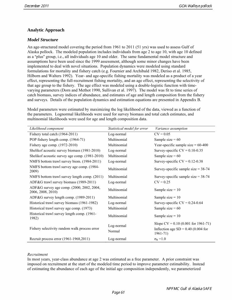
Model Structure An age-structured model covering the period from 1961 to 2011 (51 yrs) was used to assess Gulf of Alaska pollock. The modeled population includes individuals from age 2 to age 10, with age 10 defined as a Aplus@ group, i.e., all individuals age 10 and older. The same fundamental model structure and assumptions have been used since the 1999 assessment, although some minor changes have been implemented to deal with novel situations. Population dynamics were modeled using standard formulations for mortality and fishery catch (e.g. Fournier and Archibald 1982, Deriso et al. 1985, Hilborn and Walters 1992). Year- and age-specific fishing mortality was modeled as a product of a year effect, representing the full-recruitment fishing mortality, and an age effect, representing the selectivity of that age group to the fishery. The age effect was modeled using a double-logistic function with time-varying parameters (Dorn and Methot 1990, Sullivan et al. 1997). The model was fit to time series of catch biomass, survey indices of abundance, and estimates of age and length composition from the fishery and surveys. Details of the population dynamics and estimation equations are presented in Appendix B. Model parameters were estimated by maximizing the log likelihood of the data, viewed as a function of the parameters. Lognormal likelihoods were used for survey biomass and total catch estimates, and multinomial likelihoods were used for age and length composition data.

Likelihood component Statistical model for error Variance assumption Fishery total catch (1964-2011) Log-normal CV = 0.05 POP fishery length comp. (1964-71) Multinomial Sample size = 60 Fishery age comp. (1972-2010) Multinomial Year-specific sample size = 60-400 Shelikof acoustic survey biomass (1981-2010) Log-normal Survey-specific CV = 0.10-0.35 Shelikof acoustic survey age comp. (1981-2010) Multinomial Sample size = 60 NMFS bottom trawl survey biom. (1984-2011) Log-normal Survey-specific CV = 0.12-0.38 NMFS bottom trawl survey age comp. (1984-2009) Multinomial Survey-specific sample size = 38-74

NMFS bottom trawl survey length comp. (2011) Multinomial Survey-specific sample size = 38-74 ADF&G trawl survey biomass (1989-2011) Log-normal CV = 0.25 ADF&G survey age comp. (2000, 2002, 2004, 2006, 2008, 2010) Multinomial Sample size = 10

ADF&G survey length comp. (1989-2011) Multinomial Sample size = 10 Historical trawl survey biomass (1961-1982) Log-normal Survey-specific CV = 0.24-0.64 Historical trawl survey age comp. (1973) Multinomial Sample size = 60 Historical trawl survey length comp. (1961-1982) Multinomial Sample size = 10

Fishery selectivity random walk process error Log-normal Normal

Slope CV = 0.10 (0.001 for 1961-71) Inflection age SD = 0.40 (0.004 for 1961-71)

Recruit process error (1961-1968,2011) Log-normal σR =1.0 Recruitment In most years, year-class abundance at age 2 was estimated as a free parameter. A prior constraint was imposed on recruitment at the start of the modeled time period to improve parameter estimability. Instead of estimating the abundance of each age of the initial age composition independently, we parameterized

the initial age composition with mean log recruitment plus a log deviation from an equilibrium age structure based on that mean initial recruitment. A penalty was added to the log likelihood so that the log deviations would have the same variability as recruitment during the assessment period (σR =1.0). We also used the same constraint for log deviations in recruitment for 1961-68, and in 2011. Log deviations were estimated as free parameters in other years. These relatively weak constraints were sufficient to obtain fully converged parameter estimates while retaining an appropriate level of uncertainty (e.g. the CV of recruitment in 2011 ≈ σR). Modeling fishery data To accommodate changes in selectivity during the development of the fishery, we allowed the parameters of the double logistic function to vary according to a random walk process (Sullivan et al. 1997). This approach allows selectivity to vary from one year to the next, but restricts the amount of variation that can occur. The resulting selectivity patterns are similar to those obtained by grouping years, but transitions between selectivity patterns occur gradually rather than abruptly. Constraining the selectivity pattern for a group of years to be similar can be done simply by reducing the year-specific standard deviation of the process error term. Since limited data are available from the Pacific ocean perch fishery years (1964-71) and in 2011, the process error standard deviation for those years was assumed to be very small, so that annual changes in selectivity are very restricted during these years. Modeling survey data Survey abundance was assumed to be proportional to total abundance as modified by the estimated survey selectivity pattern. Expected population numbers at age for the survey were based on the mid-date of the survey, assuming constant fishing and natural mortality throughout the year. Standard deviations in the log-normal likelihood were set equal to the sampling error CV (coefficient of variation) associated with each survey estimate of abundance (Kimura 1991). Survey catchability coefficients can be fixed or freely estimated. The NMFS bottom trawl survey catchability was fixed at one in this and previous assessments as a precautionary constraint on the total biomass estimated by the model. A likelihood profile on trawl catchability showed that the maximum likelihood estimate of trawl catchability was approximately 0.68. This result is reasonable because pollock are known to form pelagic aggregations and occur in nearshore areas not well sampled by the NMFS bottom trawl survey. Catchability coefficients for other surveys were estimated as free parameters. Egg production estimates of spawning stock biomass were included in the model by setting the age-specific selectivity equal to the estimated percent mature at age estimated by Hollowed et al. (1991). The Simrad EK acoustic system has been used to estimate biomass in the acoustic surveys since 1992. Earlier surveys (1981-91) were obtained with an older Biosonics acoustic system (Table 1.7). Biomass estimates similar to the Biosonics acoustic system can be obtained using the Simrad EK when a volume backscattering (Sv) threshold of -58.5 dB is used (Hollowed et al. 1992). Because of the newer system’s lower noise level, abundance estimates since 1992 have been based on a Sv threshold of -70 dB. The Shelikof Strait acoustic survey time series was split into two periods corresponding to the two acoustic systems, and separate survey catchability coefficients were estimated for each period. For the 1992 and 1993 surveys, biomass estimates using both noise thresholds were used to provide to provide information on relative catchability. A vessel comparison (VC) experiment was conducted in March 2007 during the Shelikof Strait acoustic-trawl survey. The VC experiment involved the R/V Miller Freeman (MF, the survey vessel used to conduct Shelikof Strait surveys since the mid-1980s), and the R/V Oscar Dyson (OD), a noise-reduced survey vessel designed to conduct surveys that have traditionally been done with the R/V Miller Freeman. The vessel comparison experiment was designed to collect data either with the two vessels running beside

one another at a distance of 0.7 nmi, or with one vessel following nearly directly behind the other at a distance of about 1 nmi. The methods were similar to those used during the 2006 Bering Sea VC experiment (De Robertis et al. 2008). Results indicate that the ratio of 38 kHz pollock backscatter from the R/V Oscar Dyson relative to the R/V Miller Freeman was significantly greater than one (1.13), as would be expected if the quieter OD reduced the avoidance response of the fish. Because this difference was significant, several methods were evaluated in the 2008 assessment for incorporating this result in the assessment model. The method that was adopted was to treat the MF and the OD time series as independent survey time series, and to include the vessel comparison results directly in the log likelihood of the assessment model. This likelihood component is given by

( ) [ ] ,)log()log(2

1log 2:2 MFODMFOD

S

qqL δσ

−−−= where log(qOD) is the log catchability of the R/V Oscar Dyson, log(qMF) is the log catchability of the R/V Oscar Dyson, δOD:MF = 0.1240 is the mean of log scale paired difference in backscatter, mean[log(sAOD)-log(sAMF)] obtained from the vessel comparison, and σS = 0.0244 is the standard error of the mean. Ageing error An ageing error conversion matrix is used in the assessment model to translate model population numbers at age to expected fishery and survey catch at age (Table 1.14). Dorn et al. (2003) estimated this matrix using an ageing error model fit to the observed percent reader agreement at ages 2 and 9. Mean percent agreement is close to 100% at age 1 and declines to 40% at age 10. Annual estimates of percent agreement are variable, but show no obvious trend; hence a single conversion matrix for all years in the assessment model was adopted. The model is based on a linear increase in the standard deviation of ageing error and the assumption that ageing error is normally distributed. The model predicts percent agreement by taking into account the probability that both readers are correct, both readers are off by one year in the same direction, and both readers are off by two years in the same direction (Methot 2000). The probability that both agree and were off by more than two years was considered negligible. A recent study evaluated pollock ageing criteria using radiometric methods and found them to be unbiased (Kastelle and Kimura 2006). Length frequency data The assessment model was fit to length frequency data from various sources by converting predicted age distributions (as modified by age-specific selectivity) to predicted length distributions using an age-length conversion matrix. Because seasonal differences in pollock length at age are large, several conversion matrices were used. For each matrix, unbiased length distributions at age were estimated for several years using age-length keys, and then averaged across years. A conversion matrix estimated by Hollowed et al. (1998) was used for length-frequency data from the early period of the fishery. A conversion matrix was estimated using 1992-98 Shelikof Strait acoustic survey data and used for winter survey length frequency data. The following length bins were used: 17 - 27, 28 - 35, 36 - 42, 43 - 50, 51 - 55, 56 - 70 (cm). Finally, a conversion matrix was estimated using second and third trimester fishery age and length data during the years (1989-98) and was used for the ADF&G survey length frequency data. The following length bins were used: 25 - 34, 35 - 41, 42 - 45, 46 - 50, 51 - 55, 56 - 70 (cm), so that the first three bins would capture most of the summer length distribution of the age-2, age-3 and age-4 fish, respectively. Bin definitions were different for the summer and the winter conversion matrices to account for the seasonal growth of the younger fish (ages 2-4).

Parameters Estimated Independently Pollock life history characteristics, including natural mortality, growth, and maturity, were estimated independently. These parameters are used in the model to estimate spawning and population biomass and obtain predictions of fishery and survey biomass. Pollock life history parameters include:

• Natural mortality (M) • Proportion mature at age

• Weight at age and year by fishery and by survey

Natural mortality Hollowed and Megrey (1990) estimated natural mortality (M) using a variety of methods including estimates based on: a) growth parameters (Alverson and Carney 1975, and Pauly 1980), b) GSI (Gunderson and Dygert, 1988), c) monitoring cohort abundance, and d) estimation in the assessment model. These methods produced estimates of natural mortality that ranged from 0.24 to 0.30. The maximum age observed was 22 years. For the assessment modeling, natural mortality was assumed to be 0.3 for all ages. Hollowed et al. (2000) developed a model for Gulf of Alaska pollock that accounted for predation mortality. The model suggested that natural mortality declines from 0.8 at age 2 to 0.4 at age 5, and then remains relatively stable with increasing age. In addition, stock size was higher when predation mortality was included. In a simulation study, Clark (1999) evaluated by the effect of an erroneous M on both estimated abundance and target harvest rates for a simple age-structured model. He found that “errors in estimated abundance and target harvest rate were always in the same direction, with the result that, in the short term, extremely high exploitation rates can be recommended (unintentionally) in cases where the natural mortality rate is overestimated and historical exploitation rates in the catch-at-age data are low.” He proposed that this error could be avoided by using a conservative (low) estimate of natural mortality. This suggests that the current approach of using a potentially low but still credible estimate of M for assessment modeling is consistent with the precautionary approach. However, it should be emphasized that the role of pollock as prey in the Gulf of Alaska ecosystem cannot be fully evaluated using a single species assessment model (Hollowed et al. 2000). Maturity at age Maturity stages for female pollock describe a continuous process of ovarian development between immature and post-spawning. For the purposes of estimating a maturity vector (the proportion of an age group that has been or will be reproductively active during the year) for stock assessment, all fish greater than or equal to a particular maturity stage are assumed to be mature, while those less than that stage are assumed to be immature. Maturity stages in which ovarian development had progressed to the point where ova were distinctly visible were assumed to be mature. Maturity stages are qualitative rather than quantitative, so there is subjectivity in assigning stages, and a potential for different technicians to apply criteria differently. Because the link between pre-spawning maturity stages and eventual reproductive activity later in the season is not well established, the division between mature and immature stages is problematic. Changes in the timing of spawning could also affect maturity at age estimates. Merati (1993) compared visual maturity stages with ovary histology and a blood assay for vitellogenin and found general consistency between the different approaches. Merati (1993) noted that ovaries classified as late developing stage (i.e., immature) may contain yolked eggs, but it was unclear whether these fish would spawn later in the year. The average sample size of female pollock maturity stage data per year since 2000 from winter acoustic surveys in the Gulf of Alaska is 360 (Table 1.15).

Estimates of maturity at age in 2010 from winter acoustic surveys were above the long-term average for all ages (Fig. 1.14). Inter-annual changes in maturity at age may reflect environmental conditions, pollock population biology, effect of strong year classes moving through the population, or simply ageing error. Because there did not appear to be an objective basis for excluding data, the 1983-2010 average maturity at age was used in the assessment. Logistic regression (McCullagh and Nelder 1983) was also used to estimate the age and length at 50% maturity at age for each year. Annual estimates of age at 50% maturity are highly variable and range from 3.7 years in 1984 to 6.1 years in 1991, with an average of 4.9 years. Length at 50% mature is less variable than the age at 50% mature, suggesting that at least some of the variability in the age at maturity can be attributed to changes in length at age (Fig 1.15). Changes in year-class dominance could also potentially affect estimates of maturity at age. There is less evidence of trends in the length at 50% mature, with only the 1983 and 1984 estimates as unusually low values. The average length at 50% mature for all years is approximately 43 cm. Weight at age Year-specific weight-at-age estimates are used in the model to obtain expected catches in biomass. Where possible, year and survey-specific weight-at-age estimates are used to obtain expected survey biomass. For each data source, unbiased estimates of length at age were obtained using year-specific age-length keys. Bias-corrected parameters for the length-weight relationship, W a , were also estimated. Weights at age were estimated by multiplying length at age by the predicted weight based on the length-weight regressions. A plot of weight-at-age from the Shelikof Strait acoustic survey indicates that there has been a substantial increase in weight at age for older pollock (Fig. 1.16). For pollock greater than age 6, weight-at-age has nearly doubled since 1983-1990. Further analyses are proposed to evaluate whether these changes are a density-dependent response to declining pollock abundance, or whether they are environmentally forced. Since these changes are highly auto-correlated, a fairly sophisticated analysis would be needed to attribute causation. Changes in weight-at-age have potential implications for status determination and harvest policy. For example, if the mean weight-at-age and maturity-at-age from 1983-90 is considered representative of an unfished stock, and the current weight-at-age is attributed to a density-dependent response, current stock status would be at 51% of unfished stock size, rather than 28.8% of unfished stock size.

Lb=

Parameter Estimation A large number of parameters are estimated when using this modeling approach. More than half of these parameters are year-specific deviations in fishery selectivity coefficients. Parameters were estimated using ADModel Builder, a C++ software language extension and automatic differentiation library. Parameters in nonlinear models are estimated in ADModel Builder using automatic differentiation software extended from Greiwank and Corliss (1991) and developed into C++ class libraries. The optimizer in ADModel builder is a quasi-Newton routine (Press et al. 1992). The model is determined to have converged when the maximum parameter gradient is less than a small constant (set to 1 x 10-6). ADModel builder includes post-convergence routines to calculate standard errors (or likelihood profiles) for any quantity of interest. A list of model parameters is shown below:

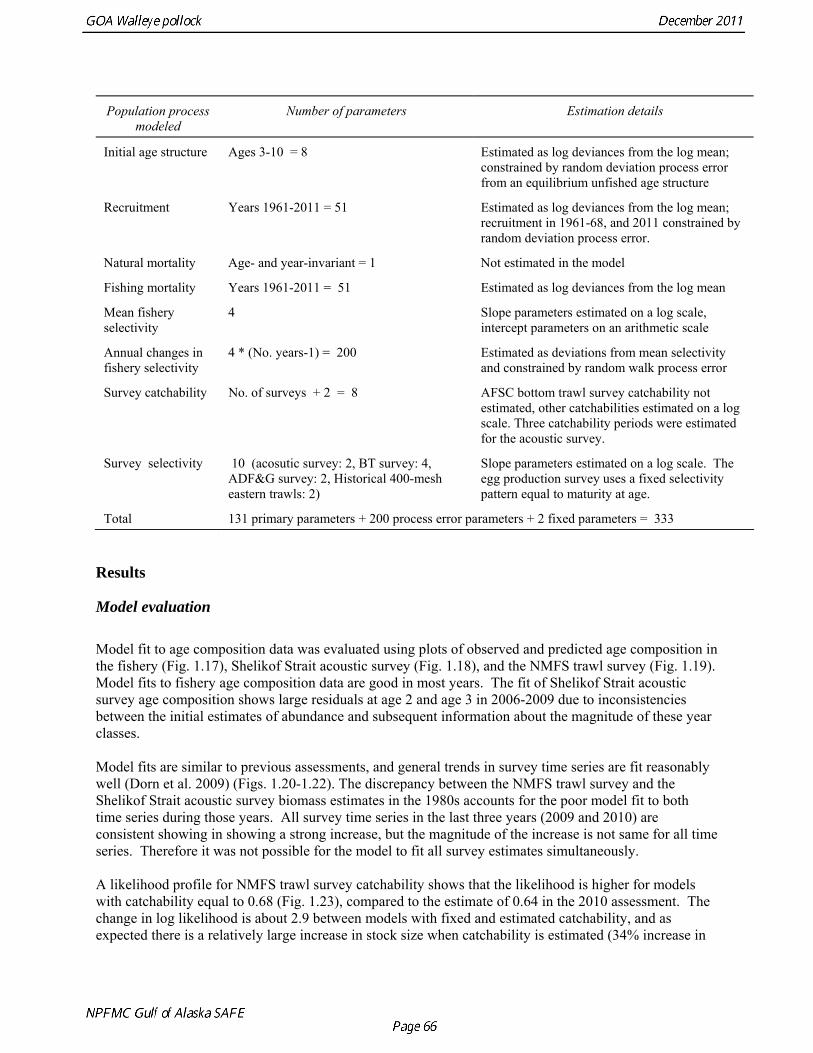
Population process modeled

Number of parameters Estimation details

Initial age structure Ages 3-10 = 8 Estimated as log deviances from the log mean; constrained by random deviation process error from an equilibrium unfished age structure

Recruitment Years 1961-2011 = 51 Estimated as log deviances from the log mean; recruitment in 1961-68, and 2011 constrained by random deviation process error.

Natural mortality Age- and year-invariant = 1 Not estimated in the model

Fishing mortality Years 1961-2011 = 51 Estimated as log deviances from the log mean

Mean fishery selectivity

4 Slope parameters estimated on a log scale, intercept parameters on an arithmetic scale

Annual changes in fishery selectivity

4 * (No. years-1) = 200 Estimated as deviations from mean selectivity and constrained by random walk process error

Survey catchability No. of surveys + 2 = 8 AFSC bottom trawl survey catchability not estimated, other catchabilities estimated on a log scale. Three catchability periods were estimated for the acoustic survey.

Survey selectivity 10 (acosutic survey: 2, BT survey: 4, ADF&G survey: 2, Historical 400-mesh eastern trawls: 2)

Slope parameters estimated on a log scale. The egg production survey uses a fixed selectivity pattern equal to maturity at age.

Total 131 primary parameters + 200 process error parameters + 2 fixed parameters = 333

Results

Model evaluation Model fit to age composition data was evaluated using plots of observed and predicted age composition in the fishery (Fig. 1.17), Shelikof Strait acoustic survey (Fig. 1.18), and the NMFS trawl survey (Fig. 1.19). Model fits to fishery age composition data are good in most years. The fit of Shelikof Strait acoustic survey age composition shows large residuals at age 2 and age 3 in 2006-2009 due to inconsistencies between the initial estimates of abundance and subsequent information about the magnitude of these year classes. Model fits are similar to previous assessments, and general trends in survey time series are fit reasonably well (Dorn et al. 2009) (Figs. 1.20-1.22). The discrepancy between the NMFS trawl survey and the Shelikof Strait acoustic survey biomass estimates in the 1980s accounts for the poor model fit to both time series during those years. All survey time series in the last three years (2009 and 2010) are consistent showing in showing a strong increase, but the magnitude of the increase is not same for all time series. Therefore it was not possible for the model to fit all survey estimates simultaneously. A likelihood profile for NMFS trawl survey catchability shows that the likelihood is higher for models with catchability equal to 0.68 (Fig. 1.23), compared to the estimate of 0.64 in the 2010 assessment. The change in log likelihood is about 2.9 between models with fixed and estimated catchability, and as expected there is a relatively large increase in stock size when catchability is estimated (34% increase in

2011 spawning biomass). These results are similar to previous assessments. To be consistent with recommendations in previous assessments, we used a base model with fixed trawl survey catchability of 1.0. Time series results Parameter estimates and model output are presented in a series of tables and figures. Estimated survey selectivity and fishery selectivity for different periods given in Table 1.16 (see also Figure 1.24). Table 1.17 gives the estimated population numbers at age for the years 1961-2011. Table 1.18 gives the estimated time series of age 3+ population biomass, age-2 recruitment, and harvest rate (catch/3+ biomass) for 1977-2010 (see also Fig. 1.25). Table 1.19 gives coefficients of variation and 95% confidence intervals for age-2 recruitment and spawning stock biomass. Stock size peaked in the early 1980s at approximately 1.1 times the proxy for unfished stock size (B100% = mean 1979-2009 recruitment multiplied by the spawning biomass per recruit in the absence of fishing (SPR at F=0)). In 1998, the stock dropped below the B40% for the first time since the 1970s, reached a minimum in 2003 of 20% of unfished stock size. Over the last five years (2007-2011) stock size has varied between 25% and 35% of unfished stock size. Retrospective comparison of assessment results A retrospective comparison of assessment results for the years 1993-2011 indicates the current estimated trend in spawning biomass for 1990-2010 is consistent with previous estimates (Fig. 1.26, top panel). All time series show a similar pattern of decreasing spawning biomass in the 1990s followed by a period of greater stability in 2000s. There appear to be no consistent pattern of bias in estimates of ending year biomass, but assessment errors are clearly correlated over time, such that there are runs of over estimates and under estimates. The estimated 2011 age composition from the current assessment is similar to projected 2011 age composition in the 2010 assessment (Fig. 1.26, bottom panel). The largest change is the estimate of the age-2 fish (2009 year class), which is about half the size of the project value of 0.7 billion (= mean recruitment) in last year’s assessment. Stock productivity Recruitment of Gulf of Alaska pollock is more variable (CV = 1.09) than Eastern Bering Sea pollock (CV = 0.62). Other North Pacific groundfish stocks, such as sablefish and Pacific ocean perch, also have high recruitment variability. However, unlike sablefish and Pacific ocean perch, pollock have a short generation time (<10 yrs), so that large year classes do not persist in the population long enough to have a buffering effect on population variability. Because of these intrinsic population characteristics, the typical pattern of biomass variability for Gulf of Alaska pollock will be sharp increases due to strong recruitment, followed by periods of gradual decline until the next strong year class recruits to the population. Gulf of Alaska pollock is more likely to show this pattern than any other groundfish stock in the North Pacific due to the combination of a short generation time and high recruitment variability. Since 1980, strong year classes have occurred every four to six years (Fig. 1.25). Because of high recruitment variability, the functional relationship between spawning biomass and recruitment is difficult to estimate despite good contrast in spawning biomass. Strong and weak year classes have been produced at high and low level of spawning biomass. The 1972 year class (one of the largest on record) was produced by an estimated spawning biomass close to current levels, suggesting that the stock has the potential to produce strong year classes. Spawner productivity is higher on average at low spawning biomass compared to high spawning biomass, indicating that survival of eggs to recruitment is density-dependent (Fig. 1.27). However, this pattern of density-dependent survival only emerges on a decadal scale, and could be confounded with environmental variability on the same temporal scale. These decadal trends in spawner productivity have produced the pattern of increase and decline in the GOA pollock

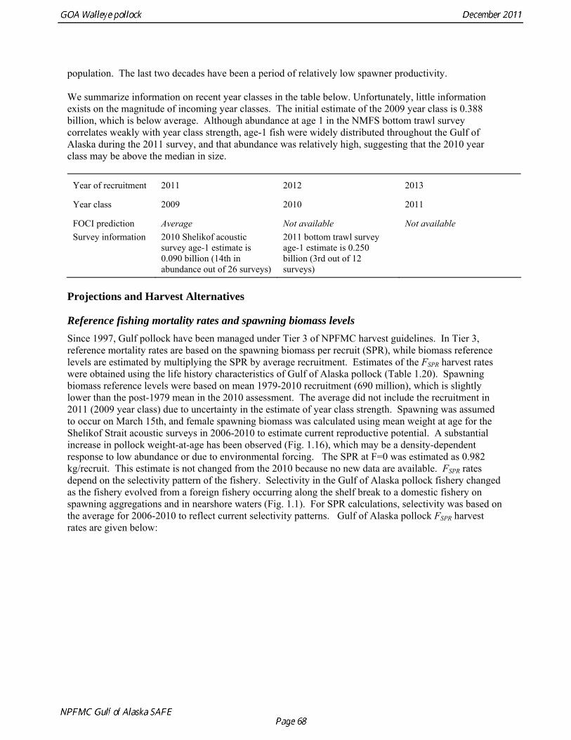
population. The last two decades have been a period of relatively low spawner productivity. We summarize information on recent year classes in the table below. Unfortunately, little information exists on the magnitude of incoming year classes. The initial estimate of the 2009 year class is 0.388 billion, which is below average. Although abundance at age 1 in the NMFS bottom trawl survey correlates weakly with year class strength, age-1 fish were widely distributed throughout the Gulf of Alaska during the 2011 survey, and that abundance was relatively high, suggesting that the 2010 year class may be above the median in size.

Year of recruitment

2011 2012 2013

Year class

2009 2010 2011

FOCI prediction

Average Not available Not available

Survey information 2010 Shelikof acoustic survey age-1 estimate is 0.090 billion (14th in abundance out of 26 surveys)

2011 bottom trawl survey age-1 estimate is 0.250 billion (3rd out of 12 surveys)

Projections and Harvest Alternatives

Reference fishing mortality rates and spawning biomass levels Since 1997, Gulf pollock have been managed under Tier 3 of NPFMC harvest guidelines. In Tier 3, reference mortality rates are based on the spawning biomass per recruit (SPR), while biomass reference levels are estimated by multiplying the SPR by average recruitment. Estimates of the FSPR harvest rates were obtained using the life history characteristics of Gulf of Alaska pollock (Table 1.20). Spawning biomass reference levels were based on mean 1979-2010 recruitment (690 million), which is slightly lower than the post-1979 mean in the 2010 assessment. The average did not include the recruitment in 2011 (2009 year class) due to uncertainty in the estimate of year class strength. Spawning was assumed to occur on March 15th, and female spawning biomass was calculated using mean weight at age for the Shelikof Strait acoustic surveys in 2006-2010 to estimate current reproductive potential. A substantial increase in pollock weight-at-age has been observed (Fig. 1.16), which may be a density-dependent response to low abundance or due to environmental forcing. The SPR at F=0 was estimated as 0.982 kg/recruit. This estimate is not changed from the 2010 because no new data are available. FSPR rates depend on the selectivity pattern of the fishery. Selectivity in the Gulf of Alaska pollock fishery changed as the fishery evolved from a foreign fishery occurring along the shelf break to a domestic fishery on spawning aggregations and in nearshore waters (Fig. 1.1). For SPR calculations, selectivity was based on the average for 2006-2010 to reflect current selectivity patterns. Gulf of Alaska pollock FSPR harvest rates are given below:

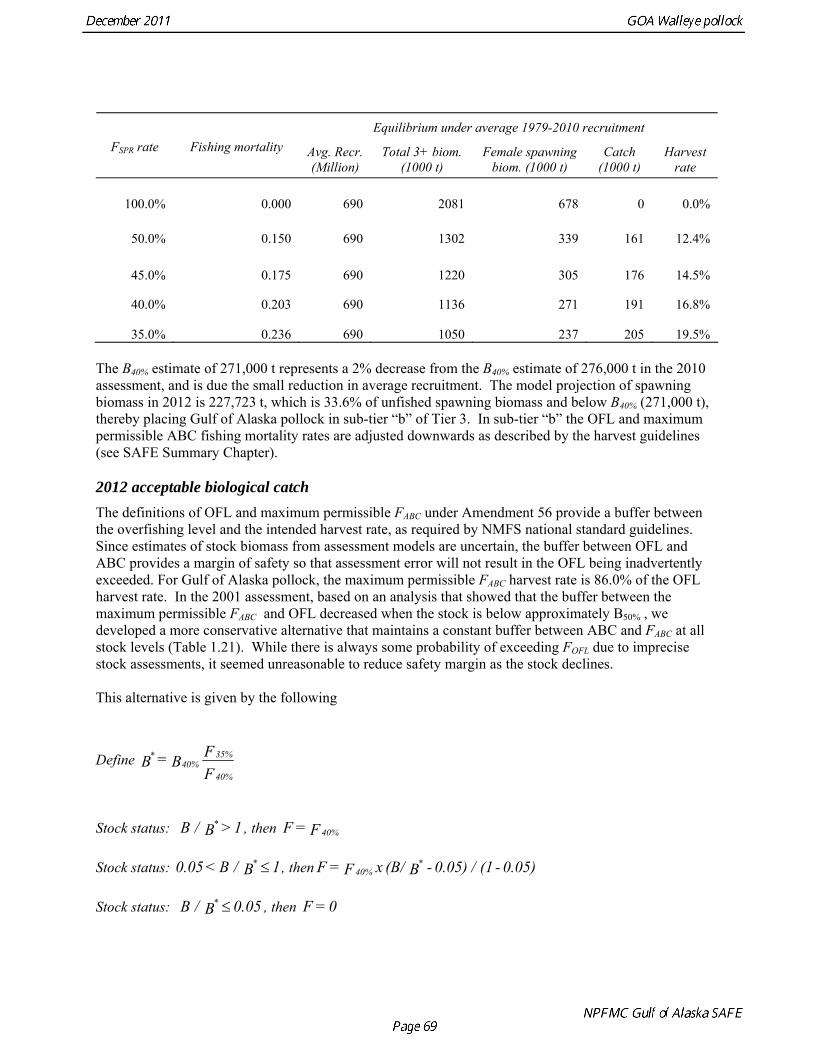
Equilibrium under average 1979-2010 recruitment

FSPR rate Fishing mortality Avg. Recr. (Million)

Total 3+ biom. (1000 t)

Female spawning biom. (1000 t)

Catch (1000 t)

Harvest rate

100.0% 0.000 690 2081 678 0 0.0%

50.0% 0.150 690 1302 339 161 12.4%

45.0% 0.175 690 1220 305 176 14.5%

40.0% 0.203 690 1136 271 191 16.8%

35.0% 0.236 690 1050 237 205 19.5% The B40% estimate of 271,000 t represents a 2% decrease from the B40% estimate of 276,000 t in the 2010 assessment, and is due the small reduction in average recruitment. The model projection of spawning biomass in 2012 is 227,723 t, which is 33.6% of unfished spawning biomass and below B40% (271,000 t), thereby placing Gulf of Alaska pollock in sub-tier “b” of Tier 3. In sub-tier “b” the OFL and maximum permissible ABC fishing mortality rates are adjusted downwards as described by the harvest guidelines (see SAFE Summary Chapter). 2012 acceptable biological catch The definitions of OFL and maximum permissible FABC under Amendment 56 provide a buffer between the overfishing level and the intended harvest rate, as required by NMFS national standard guidelines. Since estimates of stock biomass from assessment models are uncertain, the buffer between OFL and ABC provides a margin of safety so that assessment error will not result in the OFL being inadvertently exceeded. For Gulf of Alaska pollock, the maximum permissible FABC harvest rate is 86.0% of the OFL harvest rate. In the 2001 assessment, based on an analysis that showed that the buffer between the maximum permissible FABC and OFL decreased when the stock is below approximately B50% , we developed a more conservative alternative that maintains a constant buffer between ABC and FABC at all stock levels (Table 1.21). While there is always some probability of exceeding FOFL due to imprecise stock assessments, it seemed unreasonable to reduce safety margin as the stock declines. This alternative is given by the following

Define FF B = B

40%

35%40%

*

Stock status: 1 > B / B * , then F = F 40%

Stock status: 1 B / B < 0.05 * ≤ , then 0.05) - (1 / 0.05) - B(B/ xF = F *

40%

Stock status: 0.05 B / B * ≤ , then 0 = F

This alternative has the same functional form as the maximum permissible FABC; the only difference is that it declines linearly from B* ( = B47%) to 0.05B* (Fig. 1.28). Projections for 2012 for FOFL, the maximum permissible FABC, and an adjusted F40% harvest rate with a constant buffer between FABC and FOFL are given in Table 1.22. ABC recommendation There were two new surveys in 2011, the NMFS bottom trawl survey and ADF&G crab/groundfish survey. The 2011 NMFS bottom trawl survey biomass estimate was very close to the 2009 estimate (<1% increase). The ADF&G crab/groundfish survey biomass estimate declined 19% from the 2010 biomass estimate, but is 32% above the mean for 2006-2008. Recent estimates from both surveys are fit adequately by the model, and there are no large residuals to the fit to recent age data. No acoustic surveys were conducted in winter of 2011, increasing the uncertainty of the assessment model relative to previous years. The estimated abundance of mature fish in 2012 is projected to be 11% higher than in 2011, and is projected to increase gradually over the next five years. While there are concerns about the lack of Shelikof Strait acoustic survey in 2011, in the author’s opinion they do not raise to the level that precautionary reduction in the ABC is justified, especially since trends in the other data used in the assessment are reasonably consistent and consistent with model results. The recommended ABC was based on a standard model projection using the more conservative adjusted F40% harvest rate described above. The author’s recommended 2012 ABC is therefore 108,440 t, which is an increase of 22% from the 2011 ABC. While there are some elements of risk-aversion in this recommendation, such as fixing trawl catchability at 1.0, our recommendation is to delay treating those elements until an ABC framework is in place that deals explicitly with scientific uncertainty. In 2013, the ABC based an adjusted F40% harvest rate is 117,325 t (Table 1.22). The OFL in 2012 is 143,716 t, and the OFL in 2013 if the recommended ABC is taken in 2012 is 155,402 t. To evaluate the probability that the stock will drop below the B20% threshold, we projected the stock forward for five years and removed catches based on the spawning biomass in each year and the author’s recommended fishing mortality schedule. This projection incorporates uncertainty in stock status, uncertainty in the estimate of B20%, and variability in future recruitment. We then sampled from the likelihood of future spawning biomass using Markov chain Monte Carlo (MCMC) (Fig. 1.29). A chain of 1,000,000 samples was thinned by selecting every 200th sample. Analysis of the thinned MCMC chain indicates that probability of the stock dropping below B20% will be negligible in all years. Projections and Status Determination A standard set of projections is required for stocks managed under Tier 3 of Amendment 56. This set of projections encompasses seven harvest scenarios designed to satisfy the requirements of Amendment 56, the National Environmental Protection Act, and the Magnuson-Stevens Fishery Conservation and Management Act (MSFCMA). For each scenario, the projections begin with the 2011 numbers at age as estimated by the assessment model, and assume the 2011 catch will be equal to the TAC of 88,620 t. In each year, the fishing mortality rate is determined by the spawning biomass in that year and the respective harvest scenario. Recruitment is drawn from an inverse Gaussian distribution whose parameters consist of maximum likelihood estimates determined from recruitments during 1979-2010 as estimated by the assessment model. Spawning biomass is computed in each year based on the time of peak spawning (March 15) using the maturity and weight schedules in Table 1.20. This projection scheme is run 1000 times to obtain distributions of possible future stock sizes, fishing mortality rates, and catches. Five of the seven standard scenarios are used in an Environmental Assessment prepared in conjunction with the final SAFE. These five scenarios, which are designed to provide a range of harvest alternatives

that are likely to bracket the final TAC for 2012, are as follows (“max FABC” refers to the maximum permissible value of FABC under Amendment 56):

Scenario 1: In all future years, F is set equal to max FABC. (Rationale: Historically, TAC has been constrained by ABC, so this scenario provides a likely upper limit on future TACs.)

Scenario 2: In all future years, F is set equal to the FABC recommended in the assessment.

Scenario 3: In all future years, F is set equal to the five-year average F (2007-2011). (Rationale: For some stocks, TAC can be well below ABC, and recent average F may provide a better indicator of FTAC than FABC.)

Scenario 4: In all future years, F is set equal to F75%. (Rationale: This scenario represents a very conservative harvest rate and was requested by the Regional Office based on public comment.)

Scenario 5: In all future years, F is set equal to zero. (Rationale: In extreme cases, TAC may be set at a level close to zero.)

Two other scenarios are needed to satisfy the MSFCMA’s requirement to determine whether a stock is currently in an overfished condition or is approaching an overfished condition. These two scenarios are as follow (for Tier 3 stocks, the MSY level is defined as B35%):

Scenario 6: In all future years, F is set equal to FOFL. (Rationale: This scenario determines whether a stock is overfished. If the stock is expected to be 1) above its MSY level in 2011 or 2) above 1/2 of its MSY level in 2011 and above its MSY level in 2021 under this scenario, then the stock is not overfished)

Scenario 7: In 2012 and 2013, F is set equal to max FABC, and in all subsequent years, F is set equal to FOFL. (Rationale: This scenario determines whether a stock is approaching an overfished condition. If the stock is expected to be 1) above its MSY level in 2014, or 2) above 1/2 of its MSY level in 2014 and above its MSY level in 2024 under this scenario, then the stock is not approaching an overfished condition.)

Results from scenarios 1-5 are presented in Table 1.22. A Under all harvest policies, mean spawning biomass is projected remain stable or to increase gradually over the next five years (Fig. 1.30). Plots of individual projection runs are highly variable (Fig. 1.31), and may provide a more realistic view of potential pollock abundance in the future. Under the MSFCMA, the Secretary of Commerce is required to report on the status of each U.S. fishery with respect to overfishing. This report involves the answers to three questions: 1) Is the stock being subjected to overfishing? 2) Is the stock currently overfished? 3) Is the stock approaching an overfished condition? The catch estimate for the most recent complete year (2010) is 76,860 t, which is less than the 2010 OFL of 103,210 t. Therefore, the stock is not being subject to overfishing. Scenarios 6 and 7 are used to make the MSFCMA’s other required status determination as follows: Spawning biomass is estimated to be 237,607 t in 2011 which is above B35% (237,000 t). Therefore, Gulf of Alaska pollock is not currently overfished.

Under scenario 7, projected mean spawning biomass in 2014 is 224,954 t, which less than B35% , but greater than 1/2 the MSY level. In 2024, the projected mean spawning biomass is 267,397 t, which is 113% of B35% . Therefore, Gulf of Alaska pollock is not approaching an overfished condition. Ecosystem considerations

Prey of pollock An ECOPATH model was assembled to characterize food web structure in Gulf of Alaska using diet data and population estimates during 1990-93. We use ECOPATH here simply as a tool to integrate diet data and stock abundance estimates in a consistent way to evaluate ecosystem interactions. We focus primarily on first-order trophic interactions: prey of pollock and the predators of pollock. Pollock trophic interactions occur primarily in the pelagic pathway in the food web, which leads from phytoplankton through various categories of zooplankton to planktivorous fish species such as capelin and sandlance (Fig. 1.32); the primary prey of pollock are euphausiids. Pollock also consume shrimp, which are more associated with the benthic pathway, and make up approximately 18% of age 2+ pollock diet. All ages of GOA pollock are primarily zooplanktivorous during the summer growing season (>80% by weight zooplankton in diets for juveniles and adults; Fig 1.33). While there is an ontogenetic shift in diet from copepods to larger zooplankton (primarily euphausiids) and fish, cannibalism is not as prevalent in the Gulf of Alaska as in the Eastern Bering Sea, and fish consumption is low even for large pollock (Yang and Nelson 2000). There are no extended time series of zooplankton abundance for the shelf waters of the Gulf of the Alaska. Brodeur and Ware (1995) provide evidence that biomass of zooplankton in the center of the Alaska Gyre was twice as high in the 1980s than in the 1950s and 1960s, consistent with a shift to positive values of the PDO since 1977. The percentage of zooplankton in diets of pollock is relatively constant throughout the 1990s (Fig. 1.33). While indices of stomach fullness exist for these survey years, a more detailed bioenergetics modeling approach would be required to examine if feeding and growth conditions have changed over time, especially given the fluctuations in GOA water temperature in recent years (Fig. 15, Ecosystem Considerations Appendix), as water temperature has a considerable effect on digestion and other energetic rates. Predators of pollock Initial ECOPATH model results show that the top five predators on pollock >20 cm by relative importance are arrowtooth flounder, Pacific halibut, Pacific cod, Steller sea lion (SSL), and the directed pollock fishery (Fig. 1.36). For pollock less than 20cm, arrowtooth flounder represent close to 50% of total mortality. All major predators show some diet specialization, and none depend on pollock for more than 50% of their total consumption (Fig. 1.35). Pacific halibut is most dependent on pollock (48%), followed by SSL (39%), then arrowtooth flounder (24% for juvenile and adult pollock combined), and lastly Pacific cod (18%). It is important to note that although arrowtooth flounder is the largest single source of mortality for both juvenile and adult pollock (Fig 1.34), arrowtooth depend less on pollock in their diets then do the other predators. Arrowtooth consume a greater number of smaller pollock than do Pacific cod or Pacific halibut, which consume primarily adult fish. However, by weight, larger pollock are important to all three predators (Fig. 1.36). Length frequencies of pollock consumed by the western stock of Steller sea lions tend towards larger fish, and generally match the size frequencies of cod and halibut (Zeppelin et al. 2004). The diet of Pacific cod and Pacific halibut are similar in that the majority of their diet besides pollock is from the benthic pathway of the food web. Alternate prey for Steller sea lions and arrowtooth flounder are similar, and come primarily from the pelagic pathway.

Predation mortality, as estimated by ECOPATH, is extremely high for GOA pollock >20cm. Estimates for the 1990-1993 time period indicate that known sources of predation sum to 90%-120% of the total production of walleye pollock calculated from 2004 stock assessment growth and mortality rates; estimates greater than 100% may indicate a declining stock (as shown by the stock assessment trend in the early 1990s; Fig 1.37, top), or the use of mortality rates which are too low. Conversely, as >20cm pollock include a substantial number of 2-year olds, it may be that mortality rate estimates for this age range is low. In either case, predation mortality for pollock in the GOA is much greater a proportion of pollock production than as estimated by the same methods for the Bering Sea, where predation mortality (primarily pollock cannibalism) was up to 50% of total production. Aside from long-recognized decline in Steller sea lion abundance, the major predators of pollock in the Gulf of Alaska are stable to increasing, in some cases notably so since the 1980s (Fig. 1.37, top). This high level of predation is of concern in light of the declining trend of pollock with respect to predator increases. To assess this concern, it is important to determine if natural mortality may have changed over time (e.g. the shifting control hypothesis; Bailey 2000). To examine predator interactions more closely than in the initial model, diet data of major predators in trawl surveys were examined in all survey years since 1990. Trends in total consumption of walleye pollock were calculated by the following formula:

sizepredGOAsizepredsubregionsizepredsubregionsizepred RationWLFDCBnConsumptio ,,,,,,, ⋅⋅⋅= ∑ where B(pred, size, subregion) is the biomass of a predator size class in the summer groundfish surveys in a particular survey subregion; DC is the percentage by weight of pollock in that predator group as measured from stomach samples, WLF is the weight frequency of pollock in the stomachs of that predator group pooled across the GOA region, calculated from length frequencies in stomachs and length-weight relationships from the surveys. Finally, ration is an applied yearly ration for that predator group calculated by fitting weight-at-age to the generalized von Bertalanffy growth equations as described in Essington et al. (2001). Ration is assumed fixed over time for a given size class of predator. Fig. 1.37 (bottom) shows annual total estimates of consumption of pollock (all age classes) in survey years by the four major fish predators. Other predators, shown as constant, are taken from ECOPATH modeling results and displayed for comparison. Catch is shown as reported in Table 1.1. In contrast, the line in the figure shows the historical total production (tons/year) plus yearly change in biomass (positive or negative) from the stock assessment results. In a complete accounting of pollock mortality, the height of the bars should match the height of the line. As shown, estimates of consumption greatly surpass estimates of production; fishing mortality is a relatively small proportion of total consumption. Overestimates in consumption rates could arise through seasonal differences in diets; while ration is seasonally adjusted, diet proportions are based on summer data. Also, better energetic estimates of consumption would improve these estimates. In terms of the stock assessment, underestimates of production could result from underestimating natural mortality, especially at ages 2-3, underestimating the rate of decline which occurred between 1990-present, or underestimates of the total biomass of pollock; this analysis should be revisited using higher mortality at younger ages than assumed in the current stock assessment. To better judge natural mortality, consumption was calculated for two size groups of pollock, divided at 30cm fork length. This size break, which differs from the break in the ECOPATH analysis, is based on finding minima between modes of pollock in predator diets (Fig. 1.36). This break is different from the conversion matrices used in the stock assessment; perhaps due to differences in size selection between

predators and surveys. For this analysis, it is assumed that pollock<30cm are ages 0-2 while pollock ≥30cm are age 3+ fish. Consumption of age 0-2 pollock per unit predator biomass (using survey biomass) varied considerably through survey years, although within a year all predators had similar consumption levels (Fig. 1.38, top). Correlation coefficients of consumption rates were 0.98 between arrowtooth and halibut, and 0.90 for both of these species with pollock. Correlation coefficients of these three species with cod were ~0.55 for arrowtooth and halibut and ~0.20 with pollock. The majority of this predation by weight occurred on age 2 pollock. Plotted against age 2 pollock numbers calculated from the stock assessment, consumption/biomass and total consumption by predator shows a distinct pattern (Fig. 1.38, lower two graphs). In “low” recruitment years consumption is consistently low, while in high recruitment years consumption is high, but does not increase linearly, rather consumptions seems to level out at high numbers of juvenile pollock, resembling a classic “Type II” functional response. This suggests the existence bottom-up control of juvenile consumption, in which strong year classes of pollock “overwhelm” feeding rates of predators, resulting in potentially lower juvenile mortality in good recruitment years which may amplify the recruitment. However, this result should be examined iteratively within the stock assessment, as the back-calculated numbers at age 2 assume a constant natural mortality rate. Assuming a lower mortality rate due to predator satiation would lead to lower estimates of age 2 numbers, which would make the response appear more linear. Consumption of pollock ≥30cm shows a different pattern over time. A decline of consumption per unit biomass is evident for halibut and cod (Fig. 1.39, top). Arrowtooth shows an insignificant decline; it is possible that the noise in the arrowtooth trend, mirroring the consumption of <30cm fish, is due to the choice of 30cm as an age cutoff. As a function of age 3+ assessment biomass, consumption per unit biomass and total consumption remained constant as the stock declined, and then fell off rapidly at low biomass levels in recent years (Fig. 1.39, middle and bottom). Again, this result should be approached iteratively, but it suggests increasing predation mortality on age 3+ pollock during 1990-2005, possibly requiring increased foraging effort from predators. There has been a marked decline in Pacific halibut weight at age since the 1970s that Clark et al. (1999) attributed to the 1977 regime shift without being able to determine the specific biological mechanisms that produced the change. Possibilities suggested by Clark et al. (1999) include the physiological effect of an increase in temperature, intra- and interspecific competition for prey, or a change in prey quality. The two species most dependent on pollock in the early 1990s (Pacific halibut and Steller sea lion) have both shown an exceptional biological response during the post-1977 period consistent with a reduction in carrying capacity (growth for Pacific halibut, survival for Steller sea lions). In contrast, the dominant predator on pollock in the Gulf of Alaska (arrowtooth flounder) has increased steadily in abundance over the same period and shows no evidence of decline in size at age. Given that arrowtooth flounder has a range of potential prey types to select from during periods of low pollock abundance (Fig. 1.35), we do not expect that arrowtooth would decline simply due to declines in pollock. Taken together, Figs. 1.38 and 1.39 suggest that recruitment remains bottom-up controlled even under the current estimates of high predation mortality, and may lead to strong year classes. However, top-down control seems to have increased on age 3+ pollock in recent years, perhaps as predators have attempted to maintain constant pollock consumption during a period of declining abundance. It is possible that natural mortality on adult pollock will remain high in the ecosystem in spite of decreasing pollock abundance.

Ecosystem modeling To examine the relative role of pollock natural versus fishing mortality within the GOA ecosystem, a set of simulations were run using the ECOPATH model shown in Fig. 1.32. Following the method outlined in Aydin et al. (2005), 20,000 model ecosystems were drawn from distributions of input parameters; these parameter sets were subjected to a selection/rejection criteria of species persistence resulting in approximately 500 ecosystems with nondegenerate parameters. These models, which did not begin in an equilibrium state, were projected forward using ECOSIM algorithms until equilibrium conditions were reached. For each group within the model, a perturbation experiment was run in all acceptable ecosystems by reducing the species survival (increasing mortality) by 10%, or by reducing gear effort by 10%, and reporting the percent change in equilibrium of all other species or fisheries catches. The resulting changes are reported as ranges across the generated ecosystems, with 50% and 95% confidence intervals representing the distribution of percent change in equilibrium states for each perturbation. Fig. 1.40 shows the changes in other species when simulating a 10% decline in adult pollock survival (top graph), a 10% decline in juvenile pollock survival (middle graph), and a 10% decline in pollock trawl effort. Fisheries in these simulations are governed by constant fishing mortality rates rather than harvest control rules. Only the top 20 effects are shown in each graph; note the difference in scales between each graph. The model results indicate that the largest effects of declining adult pollock survival would be declines in halibut and Steller sea lion biomass. Declines in juvenile survival would have a range of effects, including halibut and Steller sea lions, but also releasing a range of competitors for zooplankton including rockfish and shrimp. The pollock trawl itself has a lesser effect throughout the ecosystem (recall that fishing mortality is small in proportion to predation mortality for pollock); the strongest modeled effects are not on competitors for prey but on incidentally caught species (Table 1.2), with the strongest effects being on sharks. The results presented above are taken from Gulfwide weighted averages of consumption; Steller sea lions and the fishing fleet are central place foragers, making foraging trips from specific locations (ports in the case of the fishing fleet, and rookeries or haulouts for Steller sea lions). Foraging bouts (or trawl sets) begin at the surface, and foragers attack their prey from the top down. For such species, directed and local changes in fishing may have a disproportionate effect compared to the results shown here. In contrast, predation by groundfish is not as constrained geographically, and captures are likely to occur when the predator swims upwards from the bottom. Changes in the vertical distribution of pollock may tend to favor one mode of foraging over another. For example, if pollock move deeper in the water column due to surface warming, foraging groundfish might obtain an advantage over surface foragers. Alternatively, pollock may respond adaptively to predation risks from groundfish or surface foragers by changing its position in the water column. Of species affecting pollock (Fig. 1.41), arrowtooth have the largest impact on adult pollock, while bottom-up processes (phytoplankton and zooplankton) have the largest impact on juvenile pollock. It is interesting to note that the link between juvenile and adult pollock is extremely uncertain (wide error bars) within these models. Finally, of the four major predators of pollock (Fig 1.42), all are affected by bottom-up forcing; Steller sea lions, Pacific cod, and Pacific halibut are all affected by pollock perturbations, while pollock effects on arrowtooth are much more minor.

Pair-wise correlations in predator trends were examined for consistent patterns (Fig. 1.43). For each pair-wise comparison, we used the maximum number of years available. Time series for Steller sea lions and Pacific cod begin in mid 1970s, while other time series extend back to the early 1960s. We make no attempt to evaluate statistical significance (biomass trends are highly autocorrelated), and emphasize that correlation does not imply causation. If two populations are strongly correlated in time, there are many possible explanations: both populations are responding to similar forcing, one or other is causative agent, etc. Pollock abundance, fishery catches, and Steller sea lions are positively correlated (Fig. 1.43). Since the harvest policy for pollock is modified fixed harvest rate strategy, a positive correlation between catch and abundance would be expected. The Steller sea lion trend is more strongly correlated with pollock abundance than pollock catches, but this correlation is based on data since 1976, and does not include earlier years of low pollock abundance. The only strong inverse correlation is between arrowtooth flounder and Steller sea lions. A strong positive correlation exists between Pacific cod and Pacific halibut, and, from the 1960s to the present, between Pacific halibut and arrowtooth flounder. Several patterns are apparent in abundance trends and the diet data. First, the two predators with alternate prey in the benthic pathway, Pacific cod and Pacific halibut, covary and have been relatively stable in the post-1977 period. Second, the long term increases in both Pacific halibut and arrowtooth flounder (with quite different diets apart from pollock) may be linked to similarities in their reproductive behavior. Both spawn offshore in late winter, and conditions that enhance onshore advection, such as El Niños, may play an important role in recruitment to nursery areas for these species (Bailey and Picquelle 2002). Finally, it is apparent that the potential for competition between Steller sea lions and arrowtooth flounder is underappreciated, perhaps because arrowtooth flounder seem poorly designed to compete as forager in the pelagic zone. However, arrowtooth flounder consume both the primary prey of Steller sea lions (pollock), and alternate pelagic prey also utilized by Steller sea lions (capelin, herring, sandlance, salmon). Arrowtooth predation on pollock occurs at a smaller size than pollock targeted by Steller sea lions. The arrowtooth flounder population is nearly unexploited, is increasing in abundance, may be increasing it’s per unit consumption of pollock, and shows no evidence of density-dependent growth. And lastly, since 1976 there has been a strong inverse correlation between arrowtooth flounder and Steller sea lion abundance that is at least consistent with competition between these species. Literature Cited

Alton, M., S. Hughes, and G. Hirschhorn. 1977. Gulf of Alaska pollock–its fisheries and resource potential. Unpubl. Manuscr., 25 p. Alaska Fisheries Science Center. National Marine Fisheries Service National Oceanic and Atmospheric Administration. 7600 Sand Point Way, NE Seattle, Washington 98115-6349. Submitted to the International North Pacific Fisheries Commission in 1977 as INPFC doc. 2019. Alton, M. S., M. O. Nelson, and B. A. Megrey. 1987. Changes in the abundance and distribution of walleye pollock (Theragra chalcogramma) in the western Gulf of Alaska. Fish. Res. 5: 185-197. Alverson, D. L. And M. J. Carney. 1975. A graphic review of the growth and decay of population cohorts. Cons. int. Explor. Mer, 133-143. Anderson, P. J. and J. F. Piatt 1999. Community reorganization in the Gulf of Alaska following ocean climate regime shift. Mar. Ecol. Prog. Ser. 189:117-123. Aydin, K., GA. McFarlane, JR. King, BA. Megrey, and KW. Myers. 2005. Linking oceanic food webs to coastal production and growth rates of Pacific salmon (Oncorhynchus spp.), using models on three scales. Deep-sea Res, II. 52: 757-780. Bailey, K.M., P.J. Stabeno, and D.A. Powers. 1997. The role of larval retention and transport features in mortality and potential gene flow of walleye pollock. J. Fish. Biol. 51(Suppl. A):135-154.

Bailey, K.M., T.J. Quinn II, P. Bentzen, and W.S. Grant. 1999. Population structure and dynamics of walleye pollock, Theragra chalcogramma. Advances in Mar. Biol. 37: 179-255. Bailey, K.M. 2000. Shifting control of recruitment of walleye pollock Theragra chalcogramma after a major climatic and ecosystem change. Mar. Ecol. Prog. Ser 198:215-224. Bailey, K. M and S. J. Picquelle. 2002. Larval distribution of offshore spawning flatfish in the Gulf of Alaska: potential transport pathways and enhanced onshore transport during ENSO events. Mar. Ecol. Prog. Ser. 236:205-217. Baranov, F.I. 1918. On the question of the biological basis of fisheries. Nauchn. Issed. Ikhtiologicheskii Inst. Izv. 1:81-128. Blackburn, J. and D. Pengilly. 1994. A summary of estimated population trends of seven most abundant groundfish species in trawl surveys conducted by Alaska Department of Fish and Game in the Kodiak and Alaska Peninsula areas, 1988 through 1993. Alaska Department of Fish and Game, Regional Information Report No. 4K94-31. 19p. Brodeur, R. D. and Ware, D.M. 1995. Interdecadal variability in distribution and catch rates of epipelagic nekton in the Northeast Pacific Ocean. pp. 329-356 in R. J. Beamish [Ed.] Climate change and northern fish populations. Canadian Special Publication of Fisheries and Aquatic Sciences 121. National Research Council of Canada, Ottawa. Kastelle, C. R. and D. K. Kimura. 2006. Age validation of walleye pollock (Theragra chalcogramma) from the Gulf of Alaska using the disequilibrium of Pb-210 and Ra-226. ICES Journal of Marine Science 63:1520-1529. Clark, W.G. 1999. Effects of an erroneous natural mortality rate on a simple age-structured model. Can. J. Fish. Aquat. Sci. 56:1721-1731. Clark, W. G., S. R. Hare, A. M. Parma, P. J. Sullivan, and R. J. Trumble. 1999. Decadal changes in growth and recruitment of Pacific halibut (Hippoglossus stenolepis). Can. J. Fish. Aquat. Sci. 56(2): 242-252. Cochran, W. G. 1977. Sampling Techniques. John Wiley and Sons. New York. 428 p. Deriso, R.B., T.J. Quinn II, and P.R. Neal. 1985. Catch-age analysis with auxiliary information. Can. J. Fish. Aquat. Sci. 42: 815-824. De Robertis, A., Hjellvik, V., Williamson, N. J., and Wilson, C. D. 2008. Silent ships do not always encounter more fish: comparison of acoustic backscatter recorded by a noise-reduced and a conventional research vessel. – ICES Journal of Marine Science, 65: 623–635. Dorn, M. W. 2004. Extending separable age-structured assessment models to evaluate trends in juvenile mortality of walleye pollock in the Gulf of Alaska. International Council for the Exploration of the Sea, CM 2004/ FF:31. Dorn, M. W., and R. D. Methot. 1990. Status of the coastal Pacific whiting resource in 1989 and recommendation to management in 1990. U.S. Dep. Commer., NOAA Tech. Memo. NMFS F/NWC-182, 84 p. Dorn, M.W. , A.B. Hollowed., E. Brown, B.A. Megrey, C. Wilson and J. Blackburn. 1999. Walleye pollock. In Stock Assessment and Fishery Evaluation Report for Groundfish Resources of the Gulf of Alaska. Prepared by the Gulf of Alaska Groundfish Plan Team, North Pacific Fishery Management Council, P.O. Box 103136, Anchorage, AK 99510. North Pacific Fisheries Management Council, Anchorage, AK. Dorn, M.W., Hollowed, A.B., E. Brown, B. Megrey, C. Wilson, and J. Blackburn. 2001. Assessment of the walleye pollock stock in the Gulf of Alaska. In Stock Assessment and Fishery Evaluation Report for Groundfish Resources of the Gulf of Alaska. Prepared by the Gulf of Alaska Groundfish Plan Team, North Pacific Fishery Management Council, P.O. Box 103136, Anchorage, AK 99510. North Pacific Fisheries Management Council, Anchorage, AK. Dorn, M.W., S. Barbeaux, B, M. Guttormsen, B. Megrey, A. Hollowed, M. Wilkins, and K. Spalinger. 2003. Assessment of the walleye pollock stock in the Gulf of Alaska. In Stock Assessment and Fishery Evaluation Report for Groundfish Resources of the Gulf of Alaska. Prepared by the Gulf of Alaska Groundfish Plan Team, North Pacific Fishery Management Council, P.O. Box 103136, Anchorage, AK 99510. North Pacific Fisheries Management Council, Anchorage, AK. Doubleday, W.G. 1976. A least-squares approach to analyzing catch at age data. Res. Bull. Int. Comm. Northw. Atl. Fish. 12:69-81.

Fournier, D. and C. P. Archibald. 1982. A general theory for analyzing catch at age data. Can. J. Fish. Aquat. Sci. 39:1195-1207. Fritz, L. W. 1993. Trawl locations of walleye pollock and Atka mackerel fisheries in the Bering Sea, Aleutian Islands, and Gulf of Alaska from 1977-92. AFSC Processed Report 93-08. NMFS, AFSC, 7600 Sand Point Way, NE, Seattle, WA 98115. 162 p. Gauthier, S. and J. K. Horne 2004. Acoustic characteristics of forage fish species in the Gulf of Alaska and Bering Sea. Can. J. Aquat. Fish. Sci. 61: 1839-1850. Grant, W.S. and F.M. Utter. 1980. Biochemical variation in walleye pollock Theragra chalcogramma: population structure in the southeastern Bering Sea and Gulf of Alaska. Can. J. Fish. Aquat. Sci. 37:1093-1100. Greiwank, A., and G.F. Corliss (eds.) 1991. Automatic differentiation of algorithms: theory, implementation and application. Proceedings of the SIAM Workshop on the Automatic Differentiation of Algorithms, held Jan. 6-8, Breckenridge, CO. Soc. Indust. and Applied Mathematics, Philadelphia. Gunderson, D. R. and P. H. Dygert. 1988. Reproductive effort as a predictor of natural mortality rate. J. Cons. int. Mer, 44:200-209. Guttormsen , M. A., C. D. Wilson, and S. Stienessen. 2001. Echo integration-trawl survey results for walleye pollock in the Gulf of Alaska during 2001. In Stock Assessment and Fishery Evaluation Report for Gulf of Alaska. Prepared by the Gulf of Alaska Groundfish Plan Team, North Pacific Fishery Management Council, P.O. Box 103136, Anchorage, AK 99510. North Pacific Fisheries Management Council, Anchorage, AK. Guttormsen , M. A., C. D. Wilson, and S. Stienessen. 2002. Echo integration-trawl survey results for walleye pollock in the Gulf of Alaska during February and March 2002. In Stock Assessment and Fishery Evaluation Report for Gulf of Alaska. Prepared by the Gulf of Alaska Groundfish Plan Team, North Pacific Fishery Management Council, P.O. Box 103136, Anchorage, AK 99510. North Pacific Fisheries Management Council, Anchorage, AK. Guttormsen , M. A., C. D. Wilson, and S. Stienessen. 2003. Results of the February and March 2003 Echo integration-trawl surveys of walleye pollock (Theragra chalcogramma) conducted in the Gulf of Alaska, Cruises MF2003-01 and MF2003-05. In Stock Assessment and Fishery Evaluation Report for Gulf of Alaska. Prepared by the Gulf of Alaska Groundfish Plan Team, North Pacific Fishery Management Council, P.O. Box 103136, Anchorage, AK 99510. North Pacific Fisheries Management Council, Anchorage, AK. Guttormsen , M. A. 2004. Results of the March-April 2004 echo integration-trawl surveys of walleye pollock (Theragra chalcogramma) conducted in the Gulf of Alaska, Cruise MF0403. In Stock Assessment and Fishery Evaluation Report for Gulf of Alaska. Prepared by the Gulf of Alaska Groundfish Plan Team, North Pacific Fishery Management Council, P.O. Box 103136, Anchorage, AK 99510. North Pacific Fisheries Management Council, Anchorage, AK. Guttormsen, M.A., A. McCarthy, and D. Jones. In review. Results of the February-March 2008 Echo Integration-Trawl Surveys of Walleye Pollock (Theragra chalcogramma) Conducted in the Gulf of Alaska, Cruises MF2008-01 and MF2008-04. AFSC Processed Rep. Alaska Fish. Sci. Cent., NOAA, Natl. Mar. Fish. Serv., 7600 Sand Point Way NE, Seattle WA 98115. Hastie, T., and R. Tibshirani. 1990. Generalized additive models. Chapman and Hall, London. 289 pp. Heifetz, J., D. Anderl, N.E. Maloney, and T.L. Rutecki. 1999. Age validation and analysis of ageing error from marked and recaptured sablefish, Anoplopoma fimbria. Fish. Bull. 97:256-263. Hilborn, R. and C.J. Walters. 1992. Quantitative fisheries stock assessment: choice, dynamics, and uncertainty. Chapman and Hall, New York, N.Y. 570 p. Hollowed, A.B. and B.A. Megrey. 1990. Walleye pollock. In Stock Assessment and Fishery Evaluation Report for the 1991 Gulf of Alaska Groundfish Fishery. Prepared by the Gulf of Alaska Groundfish Plan Team, North Pacific Fishery Management Council, P.O. Box 103136, Anchorage, AK 99510. Heino, M., U. Dieckmann, and O. R. Godø. 2002a. Estimation of reaction norms for age and size at maturation with reconstructed immature size distributions: a new technique illustrated by application to Northeast Arctic cod. ICES Journal of Marine Science 59:562–575.

Hollowed, A.B., B.A. Megrey, P. Munro, and W. Karp. 1991. Walleye pollock. In Stock Assessment and Fishery Evaluation Report for the 1992 Gulf of Alaska Groundfish Fishery. Prepared by the Gulf of Alaska Groundfish Plan Team, North Pacific Fishery Management Council, P.O. Box 103136, Anchorage, AK 99510. Hollowed, A. B., B.A. Megrey, and W. Karp. 1992. Walleye pollock. In Stock Assessment and Fishery Evaluation Report for the 1993 Gulf of Alaska Groundfish Fishery. Prepared by the Gulf of Alaska Groundfish Plan Team, North Pacific Fishery Management Council, P.O. Box 103136, Anchorage, AK 99510. Hollowed, A.B., C. Wilson, E. Brown, and B.A. Megrey. 1994. Walleye pollock. In Stock Assessment and Fishery Evaluation Report for the 1995 Gulf of Alaska Groundfish Fishery. Prepared by the Gulf of Alaska Groundfish Plan Team, North Pacific Fishery Management Council, P.O. Box 103136, Anchorage, AK 99510. Hollowed, A.B., E. Brown, P. Livingston, B.A. Megrey and C. Wilson. 1995. Walleye pollock. In Stock Assessment and Fishery Evaluation Report for Gulf of Alaska As Projected for 1996. Prepared by the Gulf of Alaska Groundfish Plan Team, North Pacific Fishery Management Council, P.O. Box 103136, Anchorage, AK 99510. North Pacific Fisheries Management Council, Anchorage, AK. Hollowed, A.B., E. Brown, J. Ianelli, B.A. Megrey and C. Wilson. 1998. Walleye pollock. In Stock Assessment and Fishery Evaluation Report for Groundfish Resources of the Gulf of Alaska. Prepared by the Gulf of Alaska Groundfish Plan Team, North Pacific Fishery Management Council, P.O. Box 103136, Anchorage, AK 99510. North Pacific Fisheries Management Council, Anchorage, AK. Hollowed, A.B., J.N. Ianelli, P. Livingston. 2000. Including predation mortality in stock assessments: a case study for Gulf of Alaska pollock. ICES J. Mar. Sci. 57:279-293. Hollowed, A.B., S. R. Hare and W. S. Wooster. 2001. Pacific Basin climate variability and patterns of Northeast Pacific marine fish production. Progress In Oceanography 49: 257-282. Hughes, S. E. and G. Hirschhorn. 1979. Biology of walleye pollock, Theragra chalcogramma, in Western Gulf of Alaska. Fish. Bull., U.S. 77:263-274. Karp, W. A. 1990. Results of echo integration midwater-trawl surveys for walleye pollock in the Gulf of Alaska in 1990. Appendix 3 of Stock Assessment and Fishery Evaluation Report for Groundfish Resources of the Gulf of Alaska. Prepared by the Gulf of Alaska Groundfish Plan Team, North Pacific Fishery Management Council, P.O. Box 103136, Anchorage, AK 99510. North Pacific Fisheries Management Council, Anchorage, AK. Kendall, A.W. Jr. and S.J. Picquelle. 1990. Egg and larval distributions of walleye pollock Theragra chalcogramma in Shelikof Strait, Gulf of Alaska. Fish. Bull., U.S. 88:133-154. Kimura, D.K. 1989. Variability, tuning, and simulation for the Doubleday-Deriso catch-at-age model. Can. J. Fish. Aquat. Sci. 46:941-949. Kimura, D.K. 1990. Approaches to age-structured separable sequential population analysis. Can. J. Fish. Aquat. Sci. 47:2364-2374. Kimura, D.K. 1991. Improved methods for separable sequential population analysis. Unpublished. Alaska Fisheries Science Center, 7600 Sand Point Way NE, Seattle, Washington 98115. Kimura, D. K. and S. Chikuni. 1989. Variability in estimating catch-in-numbers-at-age and its impact on cohort analysis. In R.J. Beamish and G.A. McFarlane (eds.), Effects of ocean variability on recruitment and an evaluation of parameters used in stock assessment models. Can. Spec. Publ. Fish. Aquat. Sci. 108:57-66. Large, W.G., and S. Pond (1982) Sensible and latent heat flux measurement over the ocean. J. Phys. Oceanogr. 2: 464-482. Lee, Y-W, Megrey, B.A., and Macklin, S.A. in prep. Using a resampling strategy to evaluate Gulf of Alaska walleye pollock recruitment forecast performance. McCullagh, P., and J. A. Nelder. 1983. Generalized linear models. Chapman and Hall, London. 261 p. McKelvey, D. 1996. Juvenile walleye pollock, Theragra chalcogramma, distribution and abundance in Shelikof Strait–What can we learn from acoustic survey results? p. 25-34. In U.S. Dep. Commer. NOAA Tech. Rep. NMFS 126.

McKelvey, D.R. 1996. Juvenile walleye pollock, Theragra chalcogramma, distribution and abundance in Shelikof Strait—what can we learn from acoustic surveys. Ecology of Juvenile Walleye Pollock, Theragra chalcogramma. NOAA Technical Report NMFS 126, p 25-34. Macklin, S.A., R.L. Brown, J. Gray, and R.W. Lindsay (1984) METLIB-II - A program library for calculating and plotting atmospheric and oceanic fields. NOAA Tech. Memo. ERL PMEL-54, NTIS PB84-205434, 53 pp. Macklin, S.A., P.J. Stabeno, and J.D. Schumacher (1993) A comparison of gradient and observed over-the-water winds along a mountainous coast. J. Geophys. Res. 98: 16,555–16,569. Megrey, B.A. 1989. Exploitation of walleye pollock resources in the Gulf of Alaska, 1964-1988: portrait of a fishery in transition. Proc. International Symp. on the Biology and Management of Walleye Pollock, Lowell Wakefield Fisheries Symp., Alaska Sea Grant Rep. 89-1, 33-58. Megrey, B.A. and Macklin, S.A. unpublished. Critical Analysis of FOCI Walleye Pollock Recruitment Prediction for the Gulf of Alaska, 1992-2005. Megrey, B.A., Lee, Y-W, and Macklin, S.A. 2005. Comparative analysis of statistical tools to identify recruitment-environment relationships and forecast recruitment strength. ICES Journal of Marine Science 62(7): 1256-1269. Merati, N. 1993. Spawning dynamics of walleye pollock, Theragra chalcogramma, in Shelikof Strait, Gulf of Alaska. Unpublished MS thesis. University of Washington. 134 p. Martin, M.H. 1997. Data Report: 1996 Gulf of Alaska bottom trawl survey. U.S. Dep. Commer., NOAA Tech. Memo. NMFS-AFSC-82, 235 p. Methot, R.D. 2000. Technical description of the stock synthesis assessment program. U.S. Dept. Commer., NOAA Tech. Memo. NMFS-NWFSC-43, 46 p. Meuter, F.J. and B.L. Norcross. 2002. Spatial and temporal patterns in the demersal fish community on the shelf and upper slope regions of the Gulf of Alaska. Fish. Bull. 100:559-581. Mulligan, T.J., Chapman, R.W. and B.L. Brown. 1992. Mitochondrial DNA analysis of walleye pollock, Theragra chalcogramma, from the eastern Bering Sea and Shelikof Strait, Gulf of Alaska. Can. J. Fish. Aquat. Sci. 49:319-326. Olsen, J.B., S.E. Merkouris, and J.E. Seeb. 2002. An examination of spatial and temporal genetic variation in walleye pollock (Theragra chalcogramma) using allozyme, mitochondrial DNA, and microsatellite data. Fish. Bull. 100:752-764. Parada, C. Hinckley, S., Dorn, M., Hermann, A.J., Megrey, B.A. submitted. Estimating walleye pollock recruitment in the Gulf of Alaska using a biophysical model: Analysis of physical processes and comparison with stock assessment models ad data. Marine Ecology Progress Series. Pauly, D.. 1980. On the interrelationships between natural mortality, growth parameters, and mean environmental temperature in 175 fish stocks. J. Cons. int. Explor. Mer, 39(2):175-192. Press, W.H., S.A. Teukolsky, W.T. Vetterling, and B.P. Flannery. 1992. Numerical recipes in C. Second ed. Cambridge University Press. 994 p. Picquelle, S.J., and B.A. Megrey. 1993. A preliminary spawning biomass estimate of walleye pollock, Theragra chalcogramma, in Shelikof Strait, Gulf of Alaska, based on the annual egg production method. Bulletin of Marine Science 53(2):728:749. Ronholt, L. L., H. H. Shippen, and E. S. Brown. 1978. Demersal fish and shellfish resources of the Gulf of Alaska from Cape Spencer to Unimak Pass 1948 - 1976 (A historical review). Northwest and Alaska Fisheries Center Processed Report. Rothschild, B. J. and Mullin, A.J. 1985. The information content of stock-and-recruitment data and its non-parametric classification. Journal du Conseil International pour l’Exploration de la Mer. 42: 116-124. Saunders, M.W., G.A. McFarlane, and W. Shaw. 1988. Delineation of walleye pollock (Theragra chalcogramma) stocks off the Pacific coast of Canada. Proc. International Symp. on the Biology and Management of Walleye Pollock, Lowell Wakefield Fisheries Symp., Alaska Sea Grant Rep. 89-1, 379-402. Schnute, J.T. and L.J. Richards. 1995. The influence of error on population estimates from catch-age models. Can. J. Fish.

Aquat. Sci. 52:2063-2077. Smith, S. J. 1990. Use of statistical models for the estimation of abundance from groundfish trawl survey data. Can. J. Fish. Aquat. Sci. 47:894-903. Somerton, D. 1979. Competitive interaction of walleye pollock and Pacific Ocean perch in the northern Gulf of Alaska. In S. J. Lipovsky and C.A. Simenstad (eds.) Gutshop '78, Fish food habits studies: Proceedings of the second Pacific Northwest Technical Workshop, held Maple Valley, WA (USA), 10-13 October, 1978., Washington Sea Grant, Seattle, WA. StatSci. 1993. S-Plus for DOS reference manual. Statistical Sciences Inc., Seattle, Wash. Sullivan, P.J., A.M. Parma, and W.G. Clark. 1997. Pacific halibut assessment: data and methods. Int. Pac. Halibut Comm. SCI. Rept. 97. 84 p. Swartzman, G., C. Huang, and S. Kaluzny. 1992. Spatial analysis of Bering Sea groundfish survey data using generalized additive models. Can. J. Fish. Aquat. Sci. 49:1366-1378. Tribuzio, C.A., S. Gaichas, J. Gasper, H. Gilroy, T. Kong, O. Ormseth, J. Cahalan, J. DiCosimo, M. Furuness, H. Shen, K. Green. 2011. Methods for the estimation of non-target species catch in the unobserved halibut IFQ fleet. August Plan Team document. Presented to the Joint Plan Teams of the North Pacific Fishery Management Council. von Szalay, P. G., and E. Brown. 2001. Trawl comparisons of fishing power differences and their applicability to National Marine Fisheries Service and the Alaska Department of Fish and Game trawl survey gear. Alaska Fishery Research Bulletin 8:85-95. Wilson, C. 1994. Echo integration-trawl survey results for pollock in the Gulf of Alaska during 1994. Appendix D of Stock Assessment and Fishery Evaluation Report for Groundfish Resources of the Gulf of Alaska. Prepared by the Gulf of Alaska Groundfish Plan Team, North Pacific Fishery Management Council, P.O. Box 103136, Anchorage, AK 99510. North Pacific Fisheries Management Council, Anchorage, AK. Wilson, C., M. Guttormsen, and D. McKelvey. 1995. Echo integration-trawl survey results for pollock in the Gulf of Alaska during 1995. Appendix D of Stock Assessment and Fishery Evaluation Report for Groundfish Resources of the Gulf of Alaska. Prepared by the Gulf of Alaska Groundfish Plan Team, North Pacific Fishery Management Council, P.O. Box 103136, Anchorage, AK 99510. North Pacific Fisheries Management Council, Anchorage, AK. Wilson, C.D., M.A. Guttormsen, and S.K. de Blois. 1996. Echo integration-trawl survey results for pollock in the Gulf of Alaska during 1996. In Stock Assessment and Fishery Evaluation Report for Groundfish Resources of the Gulf of Alaska. Prepared by the Gulf of Alaska Groundfish Plan Team, North Pacific Fishery Management Council, P.O. Box 103136, Anchorage, AK 99510. North Pacific Fisheries Management Council, Anchorage, AK. Yang, M-S. and M. W. Nelson. 2000. Food habits of the commercially important groundfishes in the Gulf of Alaska in 1990, 1993, and 1996. U.S. Dep. Commer., NOAA Tech. Memo. NMFS-AFSC-112, 174 p. Zeppelin, TK., DJ. Tollit, KA. Call, TJ. Orchard, and CJ. Gudmundson. 2004. Sizes of walleye pollock (Theragra chalcogramma) and Atka mackerel (Pleurogrammus monopterygius) consumed by the western stock of Steller sea lions (Eumetopias jubatus) in Alaska from 1998 to 2000. Fish. Bull. 102:509-521.

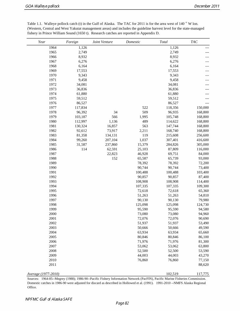
Year Foreign Joint Venture Domestic Total TAC1964 1,126 1,126 ---1965 2,749 2,749 ---1966 8,932 8,932 ---1967 6,276 6,276 ---1968 6,164 6,164 ---1969 17,553 17,553 ---1970 9,343 9,343 ---1971 9,458 9,458 ---1972 34,081 34,081 ---1973 36,836 36,836 ---1974 61,880 61,880 ---1975 59,512 59,512 ---1976 86,527 86,527 ---1977 117,834 522 118,356 150,0001978 96,392 34 509 96,935 168,8001979 103,187 566 1,995 105,748 168,8001980 112,997 1,136 489 114,622 168,8001981 130,324 16,857 563 147,744 168,8001982 92,612 73,917 2,211 168,740 168,8001983 81,358 134,131 119 215,608 256,6001984 99,260 207,104 1,037 307,401 416,6001985 31,587 237,860 15,379 284,826 305,0001986 114 62,591 25,103 87,809 116,0001987 22,823 46,928 69,751 84,0001988 152 65,587 65,739 93,0001989 78,392 78,392 72,2001990 90,744 90,744 73,4001991 100,488 100,488 103,4001992 90,857 90,857 87,4001993 108,908 108,908 114,4001994 107,335 107,335 109,3001995 72,618 72,618 65,3601996 51,263 51,263 54,8101997 90,130 90,130 79,9801998 125,098 125,098 124,7301999 95,590 95,590 94,5802000 73,080 73,080 94,9602001 72,076 72,076 90,6902002 51,937 51,937 53,4902003 50,666 50,666 49,5902004 63,934 63,934 65,6602005 80,846 80,846 86,1002006 71,976 71,976 81,3002007 53,062 53,062 63,8002008 52,500 52,500 53,5902009 44,003 44,003 43,2702010 76,860 76,860 77,1502011 88,620

Average (1977-2010) 102,519 117,775

Table 1.1. Walleye pollock catch (t) in the Gulf of Alaska. The TAC for 2011 is for the area west of 140 o W lon. (Western, Central and West Yakutat management areas) and includes the guideline harvest level for the state-managed fishery in Prince William Sound (1650 t). Research catches are reported in Appendix D.

Sources: 1964-85--Megrey (1988); 1986-90--Pacific Fishery Information Network (PacFIN), Pacific Marine Fisheries Commission. Domestic catches in 1986-90 were adjusted for discard as described in Hollowed et al. (1991). 1991-2010 --NMFS Alaska Regional Office.

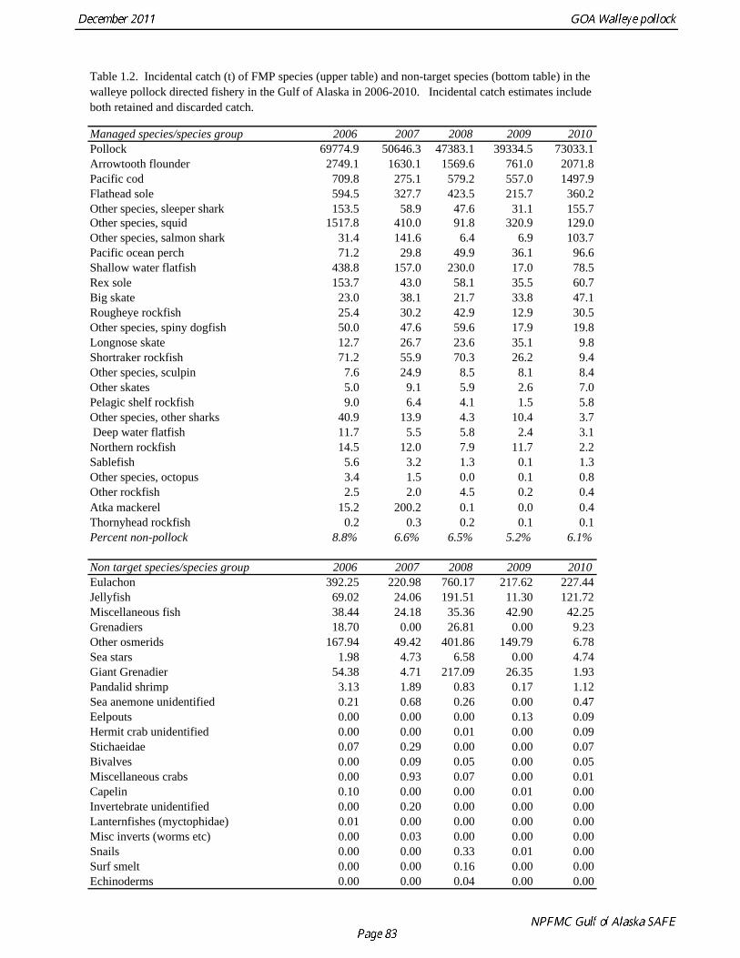
Managed species/species group 2006 2007 2008 2009 2010Pollock 69774.9 50646.3 47383.1 39334.5 73033.1Arrowtooth flounder 2749.1 1630.1 1569.6 761.0 2071.8Pacific cod 709.8 275.1 579.2 557.0 1497.9Flathead sole 594.5 327.7 423.5 215.7 360.2Other species, sleeper shark 153.5 58.9 47.6 31.1 155.7Other species, squid 1517.8 410.0 91.8 320.9 129.0Other species, salmon shark 31.4 141.6 6.4 6.9 103.7Pacific ocean perch 71.2 29.8 49.9 36.1 96.6Shallow water flatfish 438.8 157.0 230.0 17.0 78.5Rex sole 153.7 43.0 58.1 35.5 60.7Big skate 23.0 38.1 21.7 33.8 47.1Rougheye rockfish 25.4 30.2 42.9 12.9 30.5Other species, spiny dogfish 50.0 47.6 59.6 17.9 19.8Longnose skate 12.7 26.7 23.6 35.1 9.8Shortraker rockfish 71.2 55.9 70.3 26.2 9.4Other species, sculpin 7.6 24.9 8.5 8.1 8.4Other skates 5.0 9.1 5.9 2.6 7.0Pelagic shelf rockfish 9.0 6.4 4.1 1.5 5.8Other species, other sharks 40.9 13.9 4.3 10.4 3.7 Deep water flatfish 11.7 5.5 5.8 2.4 3.1Northern rockfish 14.5 12.0 7.9 11.7 2.2Sablefish 5.6 3.2 1.3 0.1 1.3Other species, octopus 3.4 1.5 0.0 0.1 0.8Other rockfish 2.5 2.0 4.5 0.2 0.4Atka mackerel 15.2 200.2 0.1 0.0 0.4Thornyhead rockfish 0.2 0.3 0.2 0.1 0.1Percent non-pollock 8.8% 6.6% 6.5% 5.2% 6.1%

Non target species/species group 2006 2007 2008 2009 2010Eulachon 392.25 220.98 760.17 217.62 227.44Jellyfish 69.02 24.06 191.51 11.30 121.72Miscellaneous fish 38.44 24.18 35.36 42.90 42.25Grenadiers 18.70 0.00 26.81 0.00 9.23Other osmerids 167.94 49.42 401.86 149.79 6.78Sea stars 1.98 4.73 6.58 0.00 4.74Giant Grenadier 54.38 4.71 217.09 26.35 1.93Pandalid shrimp 3.13 1.89 0.83 0.17 1.12Sea anemone unidentified 0.21 0.68 0.26 0.00 0.47Eelpouts 0.00 0.00 0.00 0.13 0.09Hermit crab unidentified 0.00 0.00 0.01 0.00 0.09Stichaeidae 0.07 0.29 0.00 0.00 0.07Bivalves 0.00 0.09 0.05 0.00 0.05Miscellaneous crabs 0.00 0.93 0.07 0.00 0.01Capelin 0.10 0.00 0.00 0.01 0.00Invertebrate unidentified 0.00 0.20 0.00 0.00 0.00Lanternfishes (myctophidae) 0.01 0.00 0.00 0.00 0.00Misc inverts (worms etc) 0.00 0.03 0.00 0.00 0.00Snails 0.00 0.00 0.33 0.01 0.00Surf smelt 0.00 0.00 0.16 0.00 0.00Echinoderms 0.00 0.00 0.04 0.00 0.00

Table 1.2. Incidental catch (t) of FMP species (upper table) and non-target species (bottom table) in the walleye pollock directed fishery in the Gulf of Alaska in 2006-2010. Incidental catch estimates include both retained and discarded catch.

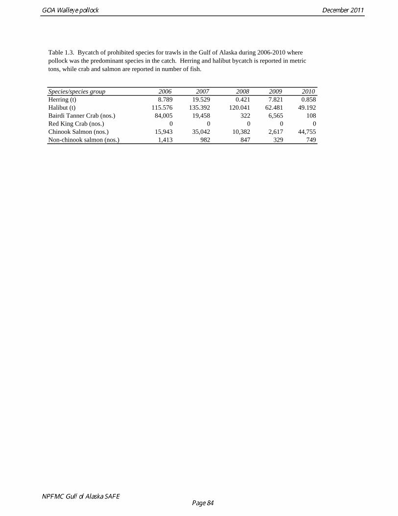
Species/species group 2006 2007 2008 2009 2010Herring (t) 8.789 19.529 0.421 7.821 0.858Halibut (t) 115.576 135.392 120.041 62.481 49.192Bairdi Tanner Crab (nos.) 84,005 19,458 322 6,565 108Red King Crab (nos.) 0 0 0 0 0Chinook Salmon (nos.) 15,943 35,042 10,382 2,617 44,755Non-chinook salmon (nos.) 1,413 982 847 329 749

Table 1.3. Bycatch of prohibited species for trawls in the Gulf of Alaska during 2006-2010 where pollock was the predominant species in the catch. Herring and halibut bycatch is reported in metric tons, while crab and salmon are reported in number of fish.

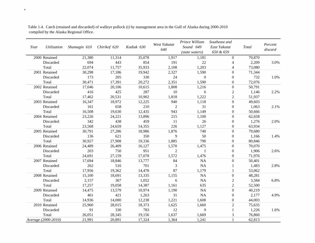
Year Utilization Shumagin 610 Chirikof 620 Kodiak 630 West Yakutat 640

Prince William Sound 649

(state waters)

Southeast and East Yakutat 650 & 659

Total Percent discard

2000 Retained 21,380 11,314 35,078 1,917 1,181 0 70,870Discarded 694 443 854 191 22 4 2,209 3.0%Total 22,074 11,757 35,933 2,108 1,203 4 73,080

2001 Retained 30,298 17,186 19,942 2,327 1,590 0 71,344Discarded 173 205 330 24 0 0 732 1.0%Total 30,471 17,391 20,272 2,351 1,590 0 72,076

2002 Retained 17,046 20,106 10,615 1,808 1,216 0 50,791Discarded 416 425 287 10 6 2 1,146 2.2%Total 17,462 20,531 10,902 1,818 1,222 2 51,937

2003 Retained 16,347 18,972 12,225 940 1,118 0 49,603Discarded 161 658 210 2 31 0 1,063 2.1%Total 16,508 19,630 12,435 943 1,149 0 50,666

2004 Retained 23,226 24,221 13,896 215 1,100 0 62,658Discarded 342 438 459 11 26 0 1,276 2.0%Total 23,568 24,659 14,355 226 1,127 0 63,934

2005 Retained 30,791 27,286 18,986 1,876 740 0 79,680Discarded 136 621 350 9 50 0 1,166 1.4%Total 30,927 27,908 19,336 1,885 790 0 80,846

2006 Retained 24,489 26,409 16,127 1,570 1,475 0 70,070Discarded 203 750 951 2 1 0 1,906 2.6%Total 24,691 27,159 17,078 1,572 1,476 0 71,976

2007 Retained 17,694 18,846 13,777 84 NA 0 50,401Discarded 262 516 701 3 NA 1 1,483 2.8%Total 17,956 19,362 14,478 87 1,179 1 53,062

2008 Retained 15,100 18,691 13,335 1,155 NA 0 48,281Discarded 2,157 367 1,052 6 NA 2 3,584 6.8%Total 17,257 19,058 14,387 1,161 635 2 52,500

2009 Retained 14,475 13,579 10,974 1,190 NA 0 40,219Discarded 461 421 1,263 31 NA 0 2,177 4.9%Total 14,936 14,000 12,238 1,221 1,608 0 44,003

2010 Retained 25,960 28,015 18,373 1,625 1,660 2 75,635Discarded 91 330 783 12 9 1 1,226 1.6%Total 26,051 28,345 19,156 1,637 1,669 3 76,860

Average (2000-2010) 21,991 20,891 17,324 1,364 1,241 1 62,813

Table 1.4. Catch (retained and discarded) of walleye pollock (t) by management area in the Gulf of Alaska during 2000-2010 compiled by the Alaska Regional Office.

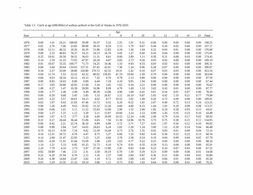
AgeYear 1 2 3 4 5 6 7 8 9 10 11 12 13 14 15 Total

1976 0.00 1.91 24.21 108.69 39.08 16.37 3.52 2.25 1.91 0.31 0.00 0.00 0.00 0.00 0.00 198.251977 0.01 2.76 7.06 23.83 89.68 30.35 8.33 2.13 1.79 0.67 0.44 0.10 0.02 0.00 0.00 167.171978 0.08 12.11 48.32 18.26 26.39 51.86 12.83 4.18 1.36 1.04 0.32 0.04 0.01 0.00 0.00 176.801979 0.00 2.53 48.83 76.37 14.15 10.13 16.70 5.02 1.27 0.60 0.16 0.04 0.00 0.00 0.00 175.811980 0.25 19.01 26.50 58.31 36.63 11.31 8.61 8.00 3.89 1.11 0.50 0.21 0.08 0.03 0.00 174.421981 0.14 2.59 31.55 73.91 47.97 20.29 4.87 4.83 2.73 0.26 0.03 0.02 0.00 0.00 0.00 189.191982 0.01 10.67 55.55 100.77 71.73 54.25 10.46 1.33 0.93 0.55 0.03 0.02 0.02 0.00 0.00 306.311983 0.00 3.64 20.64 110.03 137.31 67.41 42.01 7.38 1.24 0.06 0.28 0.07 0.00 0.00 0.00 390.071984 0.34 2.37 33.00 38.80 120.80 170.72 62.55 19.31 5.42 0.10 0.07 0.03 0.03 0.00 0.00 453.541985 0.04 12.74 5.53 33.22 42.22 86.02 128.95 41.19 10.84 2.20 0.70 0.00 0.00 0.00 0.00 363.641986 0.66 8.63 20.34 10.12 19.13 7.32 8.70 9.78 2.13 0.80 0.00 0.00 0.00 0.00 0.00 87.591987 0.00 8.83 14.03 8.00 6.89 6.44 7.18 4.19 9.95 1.94 0.00 0.00 0.00 0.00 0.00 67.441988 0.17 3.05 20.80 26.95 11.94 5.10 3.45 1.62 0.34 3.21 0.00 0.00 0.00 0.00 0.00 76.621989 1.08 0.27 1.47 19.39 28.89 16.96 8.09 4.76 1.69 1.10 3.62 0.43 0.01 0.00 0.00 87.771990 0.00 2.77 2.40 2.99 9.49 40.39 13.06 4.90 1.08 0.41 0.01 0.56 0.01 0.07 0.06 78.201991 0.00 0.59 9.68 5.45 2.85 5.33 26.67 3.12 16.10 0.87 5.65 0.42 2.19 0.21 0.77 79.901992 0.05 3.25 5.57 50.61 14.13 4.02 8.77 19.55 1.02 1.49 0.20 0.73 0.00 0.00 0.00 109.411993 0.02 1.97 9.43 21.83 47.46 15.72 6.55 6.29 8.52 1.81 2.07 0.49 0.72 0.13 0.24 123.251994 0.06 1.26 4.49 9.63 35.92 31.32 12.20 4.84 4.60 6.15 1.44 1.02 0.29 0.09 0.08 113.371995 0.00 0.06 1.01 5.11 11.52 25.83 12.09 2.99 1.52 2.00 1.82 0.19 0.28 0.03 0.15 64.611996 0.00 1.27 1.37 1.12 3.50 5.11 12.87 10.60 3.14 1.53 0.80 1.43 0.35 0.23 0.16 43.481997 0.00 1.07 6.72 3.77 3.28 6.60 10.09 16.52 12.24 5.06 2.06 0.79 0.54 0.17 0.02 68.921998 0.31 0.27 26.44 36.44 15.06 6.65 7.50 11.36 14.96 10.76 3.75 0.75 0.38 0.21 0.11 134.951999 0.00 0.42 2.21 22.74 36.10 8.99 6.89 3.72 5.71 7.27 4.01 1.07 0.56 0.12 0.10 99.922000 0.08 0.98 2.84 3.47 14.65 24.63 6.24 5.05 2.30 1.24 3.00 1.52 0.30 0.14 0.04 66.482001 0.74 10.13 6.59 7.34 9.42 12.59 14.44 4.73 2.70 1.35 0.65 0.83 0.61 0.00 0.04 72.142002 0.16 12.31 20.72 6.76 4.47 8.75 5.37 6.06 1.33 0.82 0.43 0.30 0.33 0.22 0.13 68.162003 0.14 2.69 21.47 22.95 5.33 3.25 4.66 3.76 2.58 0.54 0.19 0.04 0.09 0.04 0.05 67.792004 0.85 6.28 11.91 31.84 25.09 5.98 2.43 2.63 0.77 0.22 0.25 0.00 0.00 0.00 0.00 88.242005 1.14 1.21 5.33 6.85 41.25 21.73 6.10 0.74 0.91 0.35 0.18 0.13 0.00 0.00 0.00 85.912006 2.20 7.79 4.16 2.75 5.97 27.38 12.80 2.45 0.83 0.46 0.23 0.10 0.07 0.03 0.00 67.222007 0.82 18.89 7.46 2.51 2.31 3.58 10.19 6.70 1.59 0.29 0.23 0.09 0.00 0.00 0.01 54.682008 0.32 6.29 21.94 6.76 2.15 1.16 2.27 5.60 2.84 0.87 0.36 0.21 0.06 0.04 0.02 50.892009 0.24 6.38 14.84 13.47 3.82 1.19 0.72 0.95 1.90 1.45 0.47 0.06 0.01 0.00 0.00 45.502010 0.01 5.29 23.35 21.32 18.14 3.68 1.11 0.73 0.92 1.02 0.64 0.05 0.06 0.01 0.00 76.31

Table 1.5. Catch at age (000,000s) of walleye pollock in the Gulf of Alaska in 1976-2010.

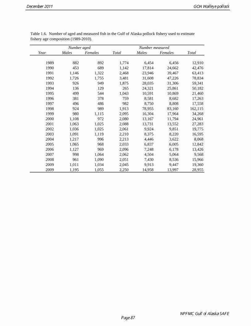
Number aged Number measuredYear Males Females Total Males Females Total

1989 882 892 1,774 6,454 6,456 12,9101990 453 689 1,142 17,814 24,662 42,4761991 1,146 1,322 2,468 23,946 39,467 63,4131992 1,726 1,755 3,481 31,608 47,226 78,8341993 926 949 1,875 28,035 31,306 59,3411994 136 129 265 24,321 25,861 50,1821995 499 544 1,043 10,591 10,869 21,4601996 381 378 759 8,581 8,682 17,2631997 496 486 982 8,750 8,808 17,5581998 924 989 1,913 78,955 83,160 162,1151999 980 1,115 2,095 16,304 17,964 34,2682000 1,108 972 2,080 13,167 11,794 24,9612001 1,063 1,025 2,088 13,731 13,552 27,2832002 1,036 1,025 2,061 9,924 9,851 19,7752003 1,091 1,119 2,210 8,375 8,220 16,5952004 1,217 996 2,213 4,446 3,622 8,0682005 1,065 968 2,033 6,837 6,005 12,8422006 1,127 969 2,096 7,248 6,178 13,4262007 998 1,064 2,062 4,504 5,064 9,5682008 961 1,090 2,051 7,430 8,536 15,9662009 1,011 1,034 2,045 9,913 9,447 19,3602009 1,195 1,055 2,250 14,958 13,997 28,955

Table 1.6. Number of aged and measured fish in the Gulf of Alaska pollock fishery used to estimate fishery age composition (1989-2010).

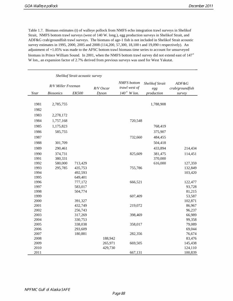
Shelikof Strait acoustic survey

NMFS bottom trawl west of 140 o W lon.

Shelikof Strait egg

production

ADF&G crab/groundfish

survey

R/V Miller Freeman R/V Oscar DysonYear Biosonics EK500

1981 2,785,755 1,788,90819821983 2,278,1721984 1,757,168 720,5481985 1,175,823 768,4191986 585,755 375,9071987 732,660 484,4551988 301,709 504,4181989 290,461 433,894 214,4341990 374,731 825,609 381,475 114,4511991 380,331 370,0001992 580,000 713,429 616,000 127,3591993 295,785 435,753 755,786 132,8491994 492,593 103,4201995 649,4011996 777,172 666,521 122,4771997 583,017 93,7281998 504,774 81,2151999 607,409 53,5872000 391,327 102,8712001 432,749 219,072 86,9672002 256,743 96,2372003 317,269 398,469 66,9892004 330,753 99,3582005 338,038 358,017 79,0892006 293,609 69,0442007 180,881 282,356 76,6742008 188,942 83,4762009 265,971 669,505 145,4382010 429,730 124,1102011 667,131 100,839

Table 1.7. Biomass estimates (t) of walleye pollock from NMFS echo integration trawl surveys in Shelikof Strait, NMFS bottom trawl surveys (west of 140 W. long.), egg production surveys in Shelikof Strait, and ADF&G crab/groundfish trawl surveys. The biomass of age-1 fish is not included in Shelikof Strait acoustic survey estimates in 1995, 2000, 2005 and 2008 (114,200, 57,300, 18,100 t and 19,090 t respectively). An adjustment of +1.05% was made to the AFSC bottom trawl biomass time series to account for unsurveyed biomass in Prince William Sound. In 2001, when the NMFS bottom trawl survey did not extend east of 147o

W lon., an expansion factor of 2.7% derived from previous surveys was used for West Yakutat.

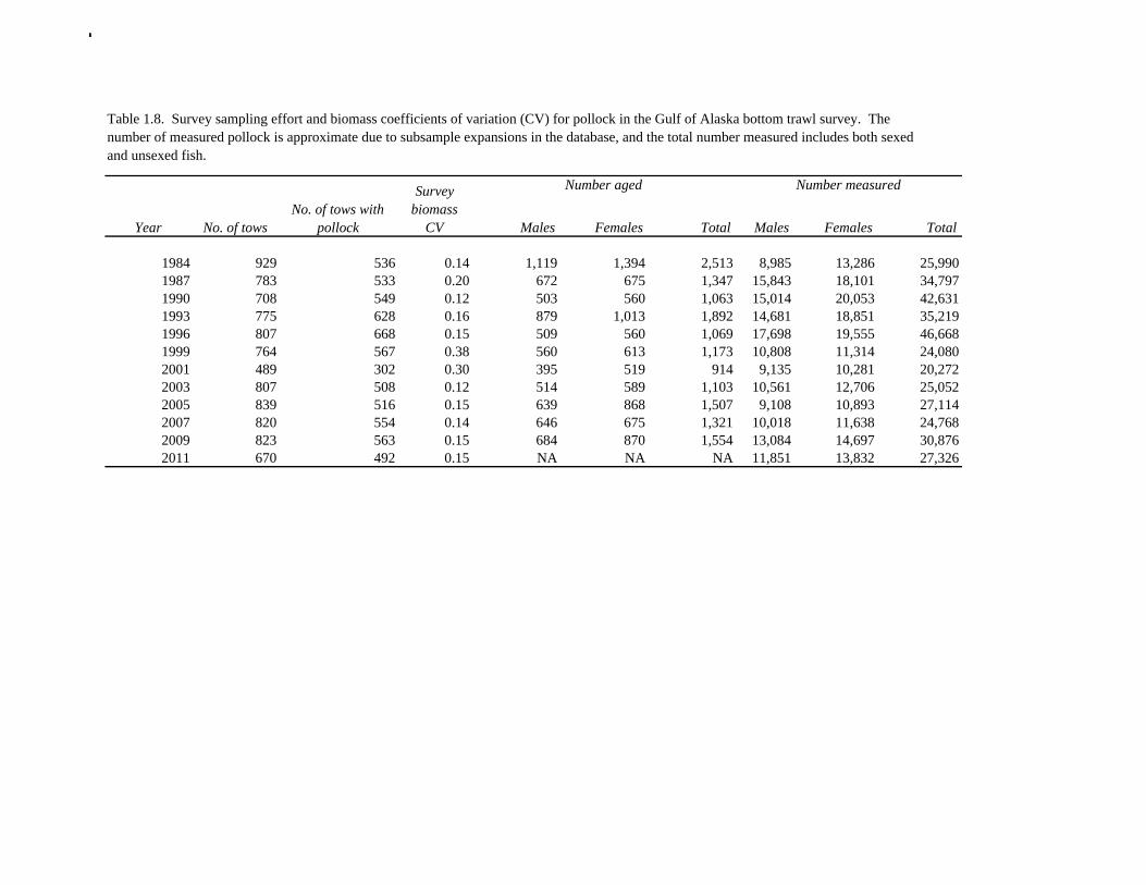
No. of towsNo. of tows with

pollock

Survey biomass

CV

Number aged Number measured

Year Males Females Total Males Females Total

1984 929 536 0.14 1,119 1,394 2,513 8,985 13,286 25,9901987 783 533 0.20 672 675 1,347 15,843 18,101 34,7971990 708 549 0.12 503 560 1,063 15,014 20,053 42,6311993 775 628 0.16 879 1,013 1,892 14,681 18,851 35,2191996 807 668 0.15 509 560 1,069 17,698 19,555 46,6681999 764 567 0.38 560 613 1,173 10,808 11,314 24,0802001 489 302 0.30 395 519 914 9,135 10,281 20,2722003 807 508 0.12 514 589 1,103 10,561 12,706 25,0522005 839 516 0.15 639 868 1,507 9,108 10,893 27,1142007 820 554 0.14 646 675 1,321 10,018 11,638 24,7682009 823 563 0.15 684 870 1,554 13,084 14,697 30,8762011 670 492 0.15 NA NA NA 11,851 13,832 27,326

Table 1.8. Survey sampling effort and biomass coefficients of variation (CV) for pollock in the Gulf of Alaska bottom trawl survey. The number of measured pollock is approximate due to subsample expansions in the database, and the total number measured includes both sexed and unsexed fish.

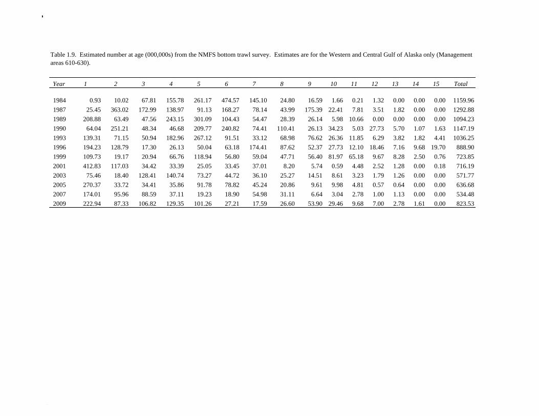
Year 1 2 3 4 5 6 7 8 9 10 11 12 13 14 15 Total

1984 0.93 10.02 67.81 155.78 261.17 474.57 145.10 24.80 16.59 1.66 0.21 1.32 0.00 0.00 0.00 1159.961987 25.45 363.02 172.99 138.97 91.13 168.27 78.14 43.99 175.39 22.41 7.81 3.51 1.82 0.00 0.00 1292.881989 208.88 63.49 47.56 243.15 301.09 104.43 54.47 28.39 26.14 5.98 10.66 0.00 0.00 0.00 0.00 1094.231990 64.04 251.21 48.34 46.68 209.77 240.82 74.41 110.41 26.13 34.23 5.03 27.73 5.70 1.07 1.63 1147.191993 139.31 71.15 50.94 182.96 267.12 91.51 33.12 68.98 76.62 26.36 11.85 6.29 3.82 1.82 4.41 1036.251996 194.23 128.79 17.30 26.13 50.04 63.18 174.41 87.62 52.37 27.73 12.10 18.46 7.16 9.68 19.70 888.901999 109.73 19.17 20.94 66.76 118.94 56.80 59.04 47.71 56.40 81.97 65.18 9.67 8.28 2.50 0.76 723.852001 412.83 117.03 34.42 33.39 25.05 33.45 37.01 8.20 5.74 0.59 4.48 2.52 1.28 0.00 0.18 716.192003 75.46 18.40 128.41 140.74 73.27 44.72 36.10 25.27 14.51 8.61 3.23 1.79 1.26 0.00 0.00 571.772005 270.37 33.72 34.41 35.86 91.78 78.82 45.24 20.86 9.61 9.98 4.81 0.57 0.64 0.00 0.00 636.682007 174.01 95.96 88.59 37.11 19.23 18.90 54.98 31.11 6.64 3.04 2.78 1.00 1.13 0.00 0.00 534.482009 222.94 87.33 106.82 129.35 101.26 27.21 17.59 26.60 53.90 29.46 9.68 7.00 2.78 1.61 0.00 823.53

Table 1.9. Estimated number at age (000,000s) from the NMFS bottom trawl survey. Estimates are for the Western and Central Gulf of Alaska only (Management areas 610-630).

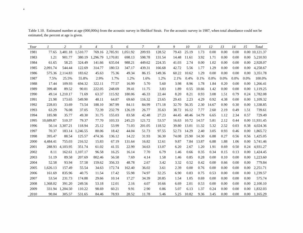
Year 1 2 3 4 5 6 7 8 9 10 11 12 13 14 15 Total1981 77.65 3,481.18 1,510.77 769.16 2,785.91 1,051.92 209.93 128.52 79.43 25.19 1.73 0.00 0.00 0.00 0.00 10,121.371983 1.21 901.77 380.19 1,296.79 1,170.81 698.13 598.78 131.54 14.48 11.61 3.92 1.71 0.00 0.00 0.00 5,210.931984 61.65 58.25 324.49 141.66 635.04 988.21 449.62 224.35 41.03 2.74 0.00 1.02 0.00 0.00 0.00 2,928.071985 2,091.74 544.44 122.69 314.77 180.53 347.17 439.31 166.68 42.72 5.56 1.77 1.29 0.00 0.00 0.00 4,258.671986 575.36 2,114.83 183.62 45.63 75.36 49.34 86.15 149.36 60.22 10.62 1.29 0.00 0.00 0.00 0.00 3,351.781987 7.5% 25.5% 55.8% 2.9% 1.7% 1.2% 1.6% 1.2% 2.1% 0.4% 0.1% 0.0% 0.0% 0.0% 0.0% 100.0%1988 17.44 109.93 694.32 322.11 77.57 16.99 5.70 5.60 3.98 8.96 1.78 1.84 0.20 0.00 0.00 1,266.411989 399.48 89.52 90.01 222.05 248.69 39.41 11.75 3.83 1.89 0.55 10.66 1.42 0.00 0.00 0.00 1,119.251990 49.14 1,210.17 71.69 63.37 115.92 180.06 46.33 22.44 8.20 8.21 0.93 3.08 1.51 0.79 0.24 1,782.081991 21.98 173.65 549.90 48.11 64.87 69.60 116.32 23.65 29.43 2.23 4.29 0.92 4.38 0.00 0.00 1,109.321992 228.03 33.69 73.54 188.10 367.99 84.11 84.99 171.18 32.70 56.35 2.30 14.67 0.90 0.30 0.00 1,338.851993 63.29 76.08 37.05 72.39 232.79 126.19 26.77 35.63 38.72 16.12 7.77 2.60 2.19 0.49 1.51 739.611994 185.98 35.77 49.30 31.75 155.03 83.58 42.48 27.23 44.45 48.46 14.79 6.65 1.12 2.34 0.57 729.491995 10,689.87 510.37 79.37 77.70 103.33 245.23 121.72 53.57 16.63 10.72 14.57 5.81 2.12 0.44 0.00 11,931.451996 56.14 3,307.21 118.94 25.12 53.99 71.03 201.05 118.52 39.80 13.01 11.32 5.32 2.52 0.03 0.38 4,024.361997 70.37 183.14 1,246.55 80.06 18.42 44.04 51.73 97.55 52.73 14.29 2.40 3.05 0.93 0.46 0.00 1,865.721998 395.47 88.54 125.57 474.36 136.12 14.22 31.93 36.30 74.08 25.90 14.30 6.88 0.27 0.56 0.56 1,425.052000 4,484.41 755.03 216.52 15.83 67.19 131.64 16.82 12.61 9.87 7.84 13.87 6.88 1.88 1.06 0.00 5,741.462001 288.93 4,103.95 351.74 61.02 41.55 22.99 34.63 13.07 6.20 2.67 1.20 1.91 0.69 0.50 0.24 4,931.272002 8.11 162.61 1,107.17 96.58 16.25 16.14 7.70 6.79 1.46 0.66 0.35 0.34 0.15 0.13 0.00 1,424.452003 51.19 89.58 207.69 802.46 56.58 7.69 4.14 1.58 1.46 0.85 0.28 0.00 0.10 0.00 0.00 1,223.602004 52.58 93.94 57.58 159.62 356.33 48.78 2.67 3.42 3.32 0.52 0.42 0.00 0.66 0.00 0.00 779.842005 1,626.13 157.49 55.54 34.63 172.74 162.40 36.02 3.61 2.39 0.00 0.76 0.00 0.00 0.00 0.00 2,251.712006 161.69 835.96 40.75 11.54 17.42 55.98 74.97 32.25 6.90 0.83 0.75 0.53 0.00 0.00 0.00 1,239.572007 53.54 231.73 174.88 29.66 10.14 17.27 34.39 20.85 1.54 1.05 0.69 0.00 0.00 0.00 0.00 575.742008 1,368.02 391.20 249.56 53.18 12.01 2.16 4.07 10.66 6.69 2.01 0.53 0.00 0.00 0.00 0.00 2,100.102009 331.94 1,204.50 110.22 98.69 60.21 9.91 2.90 0.86 5.07 6.13 1.37 0.24 0.00 0.00 0.00 1,832.032010 90.04 305.57 531.65 84.46 78.93 28.52 11.78 5.46 5.25 10.82 9.36 3.45 0.00 0.00 0.00 1,165.29

Table 1.10. Estimated number at age (000,000s) from the acoustic survey in Shelikof Strait. For the acoustic survey in 1987, when total abundance could not be estimated, the percent at age is given.

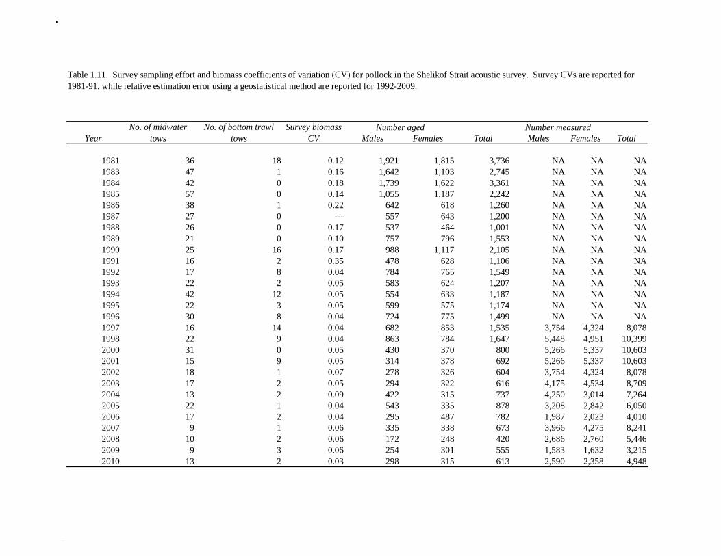
No. of midwater tows

No. of bottom trawl tows

Survey biomass CV

Number aged Number measuredYear Males Females Total Males Females Total

1981 36 18 0.12 1,921 1,815 3,736 NA NA NA1983 47 1 0.16 1,642 1,103 2,745 NA NA NA1984 42 0 0.18 1,739 1,622 3,361 NA NA NA1985 57 0 0.14 1,055 1,187 2,242 NA NA NA1986 38 1 0.22 642 618 1,260 NA NA NA1987 27 0 --- 557 643 1,200 NA NA NA1988 26 0 0.17 537 464 1,001 NA NA NA1989 21 0 0.10 757 796 1,553 NA NA NA1990 25 16 0.17 988 1,117 2,105 NA NA NA1991 16 2 0.35 478 628 1,106 NA NA NA1992 17 8 0.04 784 765 1,549 NA NA NA1993 22 2 0.05 583 624 1,207 NA NA NA1994 42 12 0.05 554 633 1,187 NA NA NA1995 22 3 0.05 599 575 1,174 NA NA NA1996 30 8 0.04 724 775 1,499 NA NA NA1997 16 14 0.04 682 853 1,535 3,754 4,324 8,0781998 22 9 0.04 863 784 1,647 5,448 4,951 10,3992000 31 0 0.05 430 370 800 5,266 5,337 10,6032001 15 9 0.05 314 378 692 5,266 5,337 10,6032002 18 1 0.07 278 326 604 3,754 4,324 8,0782003 17 2 0.05 294 322 616 4,175 4,534 8,7092004 13 2 0.09 422 315 737 4,250 3,014 7,2642005 22 1 0.04 543 335 878 3,208 2,842 6,0502006 17 2 0.04 295 487 782 1,987 2,023 4,0102007 9 1 0.06 335 338 673 3,966 4,275 8,2412008 10 2 0.06 172 248 420 2,686 2,760 5,4462009 9 3 0.06 254 301 555 1,583 1,632 3,2152010 13 2 0.03 298 315 613 2,590 2,358 4,948

Table 1.11. Survey sampling effort and biomass coefficients of variation (CV) for pollock in the Shelikof Strait acoustic survey. Survey CVs are reported for 1981-91, while relative estimation error using a geostatistical method are reported for 1992-2009.

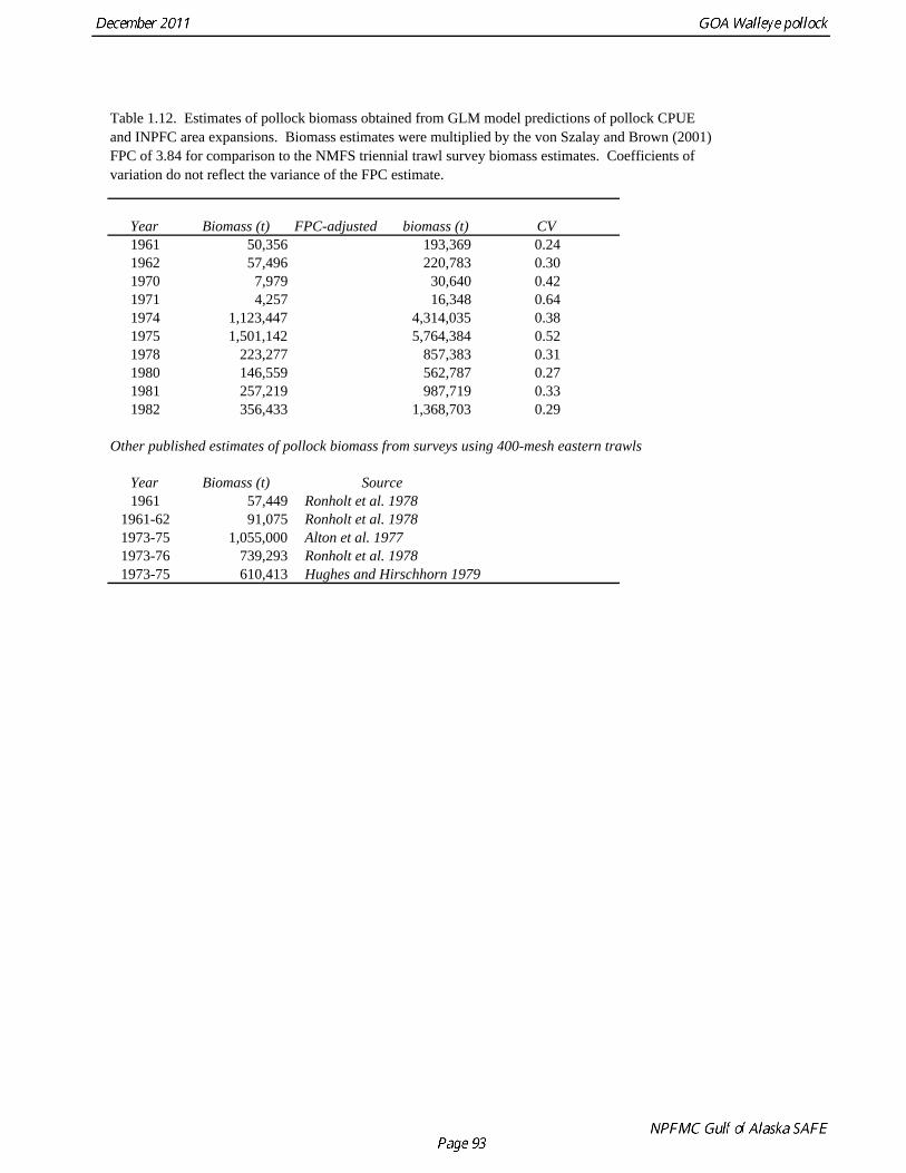
Year Biomass (t) FPC-adjusted biomass (t) CV1961 50,356 193,369 0.241962 57,496 220,783 0.301970 7,979 30,640 0.421971 4,257 16,348 0.641974 1,123,447 4,314,035 0.381975 1,501,142 5,764,384 0.521978 223,277 857,383 0.311980 146,559 562,787 0.271981 257,219 987,719 0.331982 356,433 1,368,703 0.29

Other published estimates of pollock biomass from surveys using 400-mesh eastern trawls

Year Biomass (t) Source1961 57,449 Ronholt et al. 1978

1961-62 91,075 Ronholt et al. 19781973-75 1,055,000 Alton et al. 19771973-76 739,293 Ronholt et al. 19781973-75 610,413 Hughes and Hirschhorn 1979

Table 1.12. Estimates of pollock biomass obtained from GLM model predictions of pollock CPUE and INPFC area expansions. Biomass estimates were multiplied by the von Szalay and Brown (2001) FPC of 3.84 for comparison to the NMFS triennial trawl survey biomass estimates. Coefficients of variation do not reflect the variance of the FPC estimate.

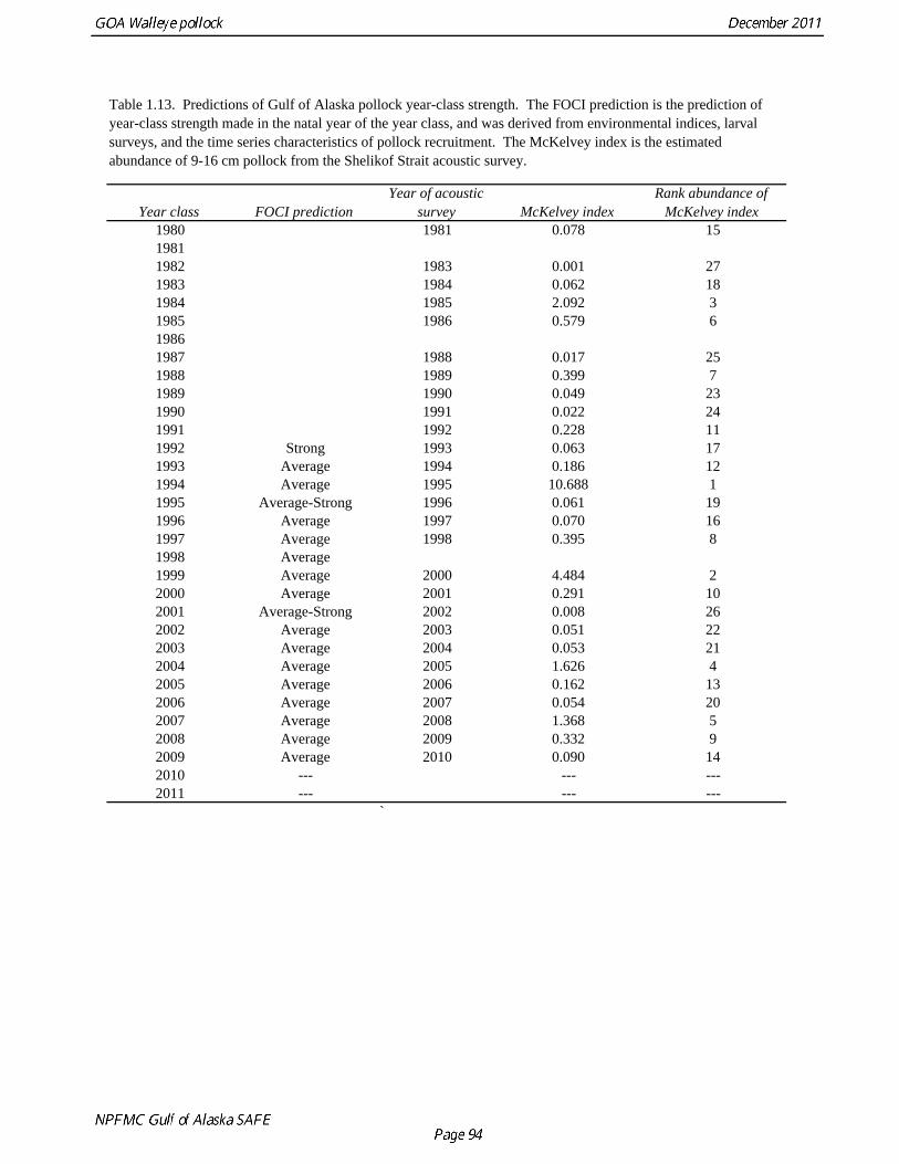
Year class FOCI predictionYear of acoustic

survey McKelvey indexRank abundance of

McKelvey index1980 1981 0.078 1519811982 1983 0.001 271983 1984 0.062 181984 1985 2.092 31985 1986 0.579 619861987 1988 0.017 251988 1989 0.399 71989 1990 0.049 231990 1991 0.022 241991 1992 0.228 111992 Strong 1993 0.063 171993 Average 1994 0.186 121994 Average 1995 10.688 11995 Average-Strong 1996 0.061 191996 Average 1997 0.070 161997 Average 1998 0.395 81998 Average1999 Average 2000 4.484 22000 Average 2001 0.291 102001 Average-Strong 2002 0.008 262002 Average 2003 0.051 222003 Average 2004 0.053 212004 Average 2005 1.626 42005 Average 2006 0.162 132006 Average 2007 0.054 202007 Average 2008 1.368 52008 Average 2009 0.332 92009 Average 2010 0.090 142010 --- --- ---2011 --- --- ---

`

Table 1.13. Predictions of Gulf of Alaska pollock year-class strength. The FOCI prediction is the prediction of year-class strength made in the natal year of the year class, and was derived from environmental indices, larval surveys, and the time series characteristics of pollock recruitment. The McKelvey index is the estimated abundance of 9-16 cm pollock from the Shelikof Strait acoustic survey.

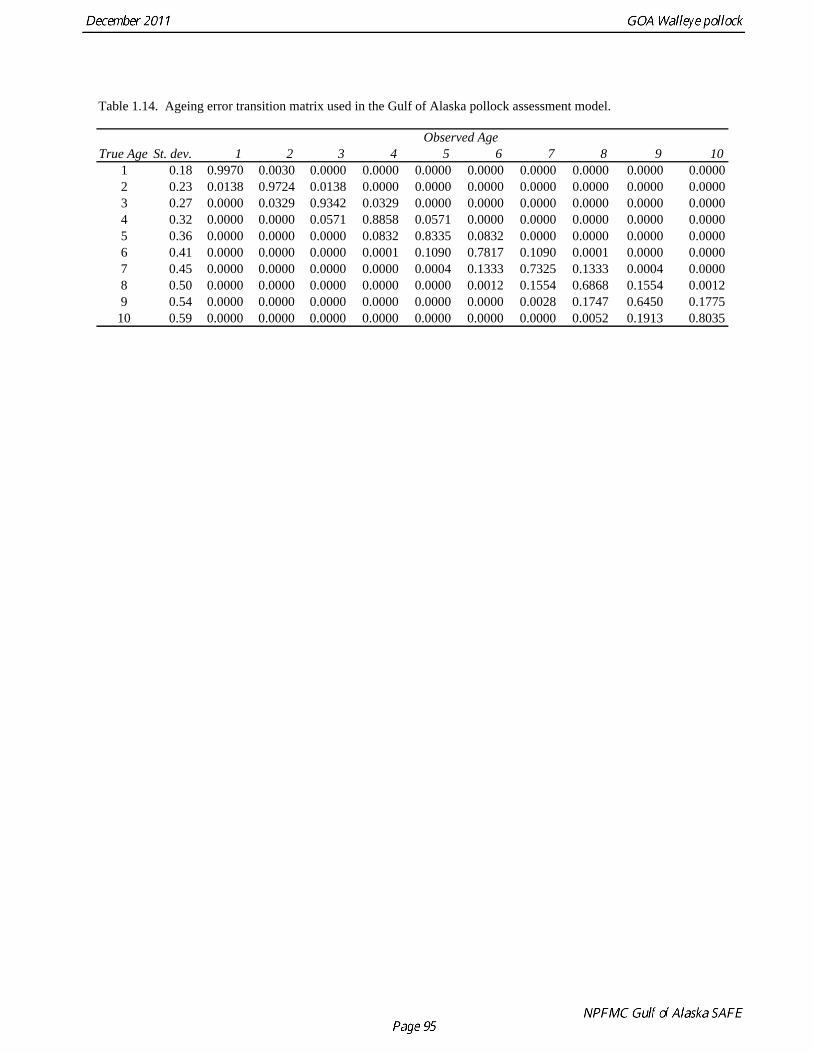
True Age St. dev.Observed Age

1 2 3 4 5 6 7 8 9 101 0.18 0.9970 0.0030 0.0000 0.0000 0.0000 0.0000 0.0000 0.0000 0.0000 0.00002 0.23 0.0138 0.9724 0.0138 0.0000 0.0000 0.0000 0.0000 0.0000 0.0000 0.00003 0.27 0.0000 0.0329 0.9342 0.0329 0.0000 0.0000 0.0000 0.0000 0.0000 0.00004 0.32 0.0000 0.0000 0.0571 0.8858 0.0571 0.0000 0.0000 0.0000 0.0000 0.00005 0.36 0.0000 0.0000 0.0000 0.0832 0.8335 0.0832 0.0000 0.0000 0.0000 0.00006 0.41 0.0000 0.0000 0.0000 0.0001 0.1090 0.7817 0.1090 0.0001 0.0000 0.00007 0.45 0.0000 0.0000 0.0000 0.0000 0.0004 0.1333 0.7325 0.1333 0.0004 0.00008 0.50 0.0000 0.0000 0.0000 0.0000 0.0000 0.0012 0.1554 0.6868 0.1554 0.00129 0.54 0.0000 0.0000 0.0000 0.0000 0.0000 0.0000 0.0028 0.1747 0.6450 0.1775

10 0.59 0.0000 0.0000 0.0000 0.0000 0.0000 0.0000 0.0000 0.0052 0.1913 0.8035

Table 1.14. Ageing error transition matrix used in the Gulf of Alaska pollock assessment model.

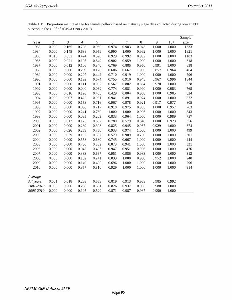
Year 2 3 4 5 6 7 8 9 10+Sample

size1983 0.000 0.165 0.798 0.960 0.974 0.983 0.943 1.000 1.000 13331984 0.000 0.145 0.688 0.959 0.990 1.000 0.992 1.000 1.000 16211985 0.015 0.051 0.424 0.520 0.929 0.992 0.992 1.000 1.000 11831986 0.000 0.021 0.105 0.849 0.902 0.959 1.000 1.000 1.000 6181987 0.000 0.012 0.106 0.340 0.769 0.885 0.950 0.991 1.000 6381988 0.000 0.000 0.209 0.176 0.606 0.667 1.000 0.857 0.964 4641989 0.000 0.000 0.297 0.442 0.710 0.919 1.000 1.000 1.000 7961990 0.000 0.000 0.192 0.674 0.755 0.910 0.945 0.967 0.996 18441991 0.000 0.000 0.111 0.082 0.567 0.802 0.864 0.978 1.000 6281992 0.000 0.000 0.040 0.069 0.774 0.981 0.990 1.000 0.983 7651993 0.000 0.016 0.120 0.465 0.429 0.804 0.968 1.000 0.985 6241994 0.000 0.007 0.422 0.931 0.941 0.891 0.974 1.000 1.000 8721995 0.000 0.000 0.153 0.716 0.967 0.978 0.921 0.917 0.977 8051996 0.000 0.000 0.036 0.717 0.918 0.975 0.963 1.000 0.957 7631997 0.000 0.000 0.241 0.760 1.000 1.000 0.996 1.000 1.000 8431998 0.000 0.000 0.065 0.203 0.833 0.964 1.000 1.000 0.989 7572000 0.000 0.012 0.125 0.632 0.780 0.579 0.846 1.000 0.923 3562001 0.000 0.000 0.289 0.308 0.825 0.945 0.967 0.929 1.000 3742002 0.000 0.026 0.259 0.750 0.933 0.974 1.000 1.000 1.000 4992003 0.000 0.029 0.192 0.387 0.529 0.909 0.750 1.000 1.000 3012004 0.000 0.000 0.558 0.680 0.745 0.667 1.000 1.000 1.000 4442005 0.000 0.000 0.706 0.882 0.873 0.941 1.000 1.000 1.000 3212006 0.000 0.000 0.043 0.483 0.947 0.951 0.986 1.000 1.000 4762007 0.000 0.000 0.333 0.667 0.951 0.986 0.983 1.000 1.000 3132008 0.000 0.000 0.102 0.241 0.833 1.000 0.968 0.952 1.000 2402009 0.000 0.000 0.140 0.400 0.696 1.000 1.000 1.000 1.000 2962010 0.000 0.000 0.357 0.810 0.929 1.000 1.000 1.000 1.000 314

AverageAll years 0.001 0.018 0.263 0.559 0.819 0.913 0.963 0.985 0.9922001-2010 0.000 0.006 0.298 0.561 0.826 0.937 0.965 0.988 1.0002006-2010 0.000 0.000 0.195 0.520 0.871 0.987 0.987 0.990 1.000

Table 1.15. Proportion mature at age for female pollock based on maturity stage data collected during winter EIT surveys in the Gulf of Alaska (1983-2010).

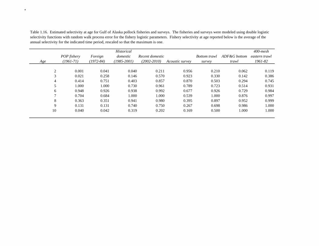
AgePOP fishery (1961-71)

Foreign (1972-84)

Historical domestic

(1985-2001)Recent domestic

(2002-2010) Acoustic survey

Bottom trawl survey

ADF&G bottom trawl

400-mesh eastern trawl

1961-82

2 0.001 0.041 0.040 0.211 0.956 0.210 0.062 0.1193 0.021 0.258 0.146 0.570 0.923 0.330 0.142 0.3864 0.414 0.751 0.403 0.857 0.870 0.503 0.294 0.7455 1.000 1.000 0.730 0.961 0.789 0.723 0.514 0.9316 0.948 0.926 0.938 0.992 0.677 0.926 0.729 0.9847 0.704 0.684 1.000 1.000 0.539 1.000 0.876 0.9978 0.363 0.351 0.941 0.980 0.395 0.897 0.952 0.9999 0.131 0.131 0.740 0.750 0.267 0.698 0.986 1.000

10 0.040 0.042 0.319 0.202 0.169 0.500 1.000 1.000

Table 1.16. Estimated selectivity at age for Gulf of Alaska pollock fisheries and surveys. The fisheries and surveys were modeled using double logistic selectivity functions with random walk process error for the fishery logistic parameters. Fishery selectivity at age reported below is the average of the annual selectivity for the indicated time period, rescaled so that the maximum is one.

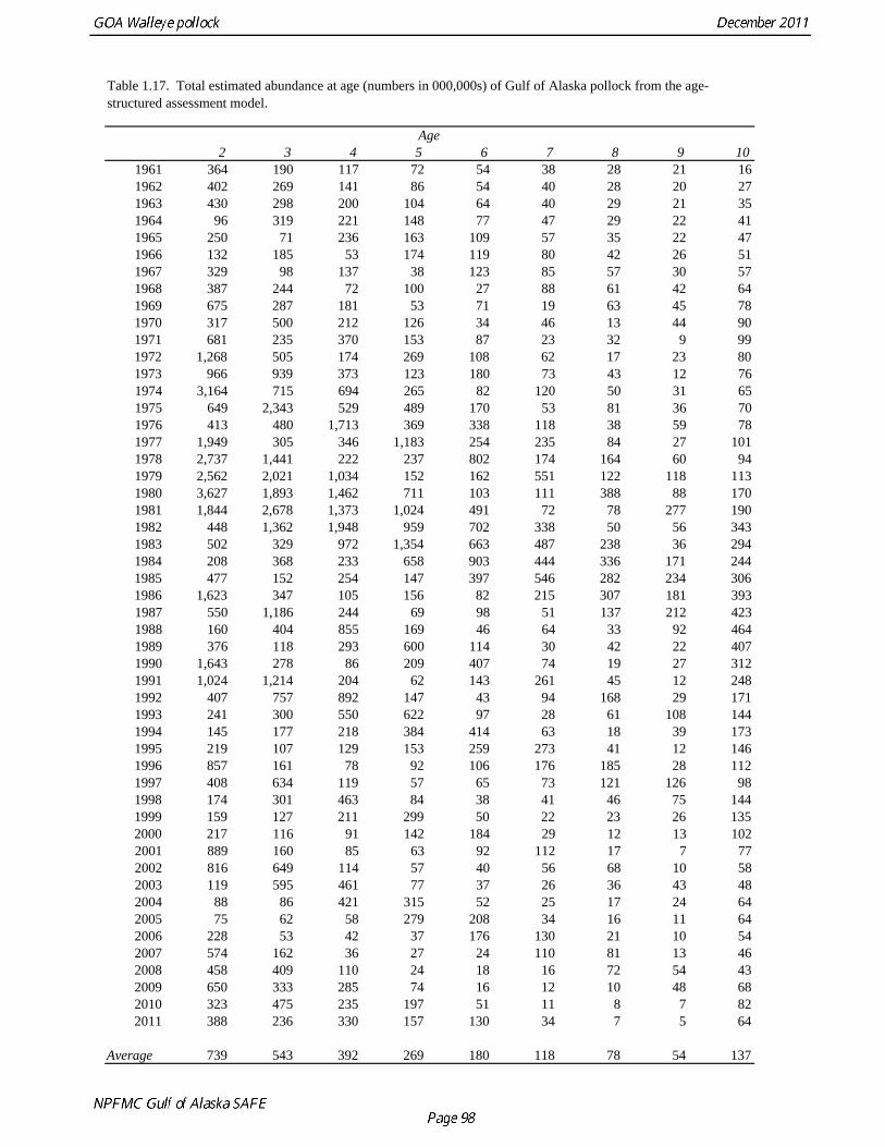
Age2 3 4 5 6 7 8 9 10

1961 364 190 117 72 54 38 28 21 161962 402 269 141 86 54 40 28 20 271963 430 298 200 104 64 40 29 21 351964 96 319 221 148 77 47 29 22 411965 250 71 236 163 109 57 35 22 471966 132 185 53 174 119 80 42 26 511967 329 98 137 38 123 85 57 30 571968 387 244 72 100 27 88 61 42 641969 675 287 181 53 71 19 63 45 781970 317 500 212 126 34 46 13 44 901971 681 235 370 153 87 23 32 9 991972 1,268 505 174 269 108 62 17 23 801973 966 939 373 123 180 73 43 12 761974 3,164 715 694 265 82 120 50 31 651975 649 2,343 529 489 170 53 81 36 701976 413 480 1,713 369 338 118 38 59 781977 1,949 305 346 1,183 254 235 84 27 1011978 2,737 1,441 222 237 802 174 164 60 941979 2,562 2,021 1,034 152 162 551 122 118 1131980 3,627 1,893 1,462 711 103 111 388 88 1701981 1,844 2,678 1,373 1,024 491 72 78 277 1901982 448 1,362 1,948 959 702 338 50 56 3431983 502 329 972 1,354 663 487 238 36 2941984 208 368 233 658 903 444 336 171 2441985 477 152 254 147 397 546 282 234 3061986 1,623 347 105 156 82 215 307 181 3931987 550 1,186 244 69 98 51 137 212 4231988 160 404 855 169 46 64 33 92 4641989 376 118 293 600 114 30 42 22 4071990 1,643 278 86 209 407 74 19 27 3121991 1,024 1,214 204 62 143 261 45 12 2481992 407 757 892 147 43 94 168 29 1711993 241 300 550 622 97 28 61 108 1441994 145 177 218 384 414 63 18 39 1731995 219 107 129 153 259 273 41 12 1461996 857 161 78 92 106 176 185 28 1121997 408 634 119 57 65 73 121 126 981998 174 301 463 84 38 41 46 75 1441999 159 127 211 299 50 22 23 26 1352000 217 116 91 142 184 29 12 13 1022001 889 160 85 63 92 112 17 7 772002 816 649 114 57 40 56 68 10 582003 119 595 461 77 37 26 36 43 482004 88 86 421 315 52 25 17 24 642005 75 62 58 279 208 34 16 11 642006 228 53 42 37 176 130 21 10 542007 574 162 36 27 24 110 81 13 462008 458 409 110 24 18 16 72 54 432009 650 333 285 74 16 12 10 48 682010 323 475 235 197 51 11 8 7 822011 388 236 330 157 130 34 7 5 64

Average 739 543 392 269 180 118 78 54 137

Table 1.17. Total estimated abundance at age (numbers in 000,000s) of Gulf of Alaska pollock from the age-structured assessment model.

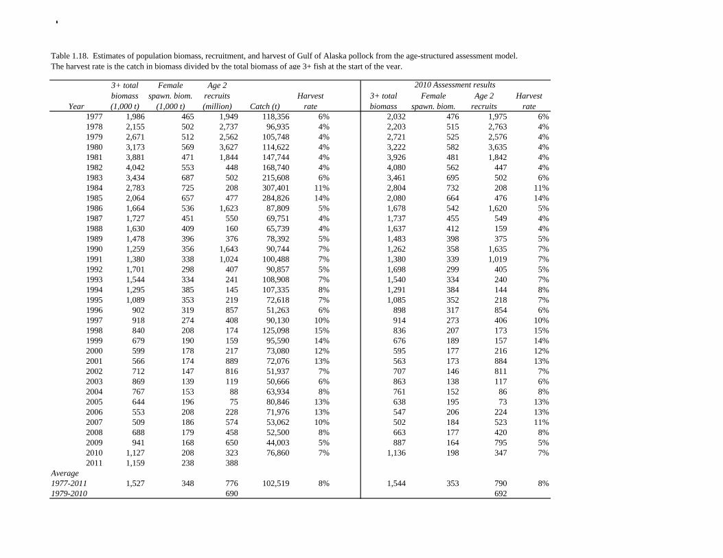
3+ total biomass

Female spawn. biom.

Age 2 recruits

Harvest rate

1977 1,986 465 1,949 118,356 6% 2,032 476 1,975 6%1978 2,155 502 2,737 96,935 4% 2,203 515 2,763 4%1979 2,671 512 2,562 105,748 4% 2,721 525 2,576 4%1980 3,173 569 3,627 114,622 4% 3,222 582 3,635 4%1981 3,881 471 1,844 147,744 4% 3,926 481 1,842 4%1982 4,042 553 448 168,740 4% 4,080 562 447 4%1983 3,434 687 502 215,608 6% 3,461 695 502 6%1984 2,783 725 208 307,401 11% 2,804 732 208 11%1985 2,064 657 477 284,826 14% 2,080 664 476 14%1986 1,664 536 1,623 87,809 5% 1,678 542 1,620 5%1987 1,727 451 550 69,751 4% 1,737 455 549 4%1988 1,630 409 160 65,739 4% 1,637 412 159 4%1989 1,478 396 376 78,392 5% 1,483 398 375 5%1990 1,259 356 1,643 90,744 7% 1,262 358 1,635 7%1991 1,380 338 1,024 100,488 7% 1,380 339 1,019 7%1992 1,701 298 407 90,857 5% 1,698 299 405 5%1993 1,544 334 241 108,908 7% 1,540 334 240 7%1994 1,295 385 145 107,335 8% 1,291 384 144 8%1995 1,089 353 219 72,618 7% 1,085 352 218 7%1996 902 319 857 51,263 6% 898 317 854 6%1997 918 274 408 90,130 10% 914 273 406 10%1998 840 208 174 125,098 15% 836 207 173 15%1999 679 190 159 95,590 14% 676 189 157 14%2000 599 178 217 73,080 12% 595 177 216 12%2001 566 174 889 72,076 13% 563 173 884 13%2002 712 147 816 51,937 7% 707 146 811 7%2003 869 139 119 50,666 6% 863 138 117 6%2004 767 153 88 63,934 8% 761 152 86 8%2005 644 196 75 80,846 13% 638 195 73 13%2006 553 208 228 71,976 13% 547 206 224 13%2007 509 186 574 53,062 10% 502 184 523 11%2008 688 179 458 52,500 8% 663 177 420 8%2009 941 168 650 44,003 5% 887 164 795 5%2010 1,127 208 323 76,860 7% 1,136 198 347 7%2011 1,159 238 388

Average1977-2011 1,527 348 776 102,519 8% 1,544 353 790 8%1979-2010 690 692

Year

2010 Assessment results3+ total biomass (1,000 t)

Female spawn. biom.

(1,000 t)

Age 2 recruits (million) Catch (t)

Harvest rate

Table 1.18. Estimates of population biomass, recruitment, and harvest of Gulf of Alaska pollock from the age-structured assessment model. The harvest rate is the catch in biomass divided by the total biomass of age 3+ fish at the start of the year.

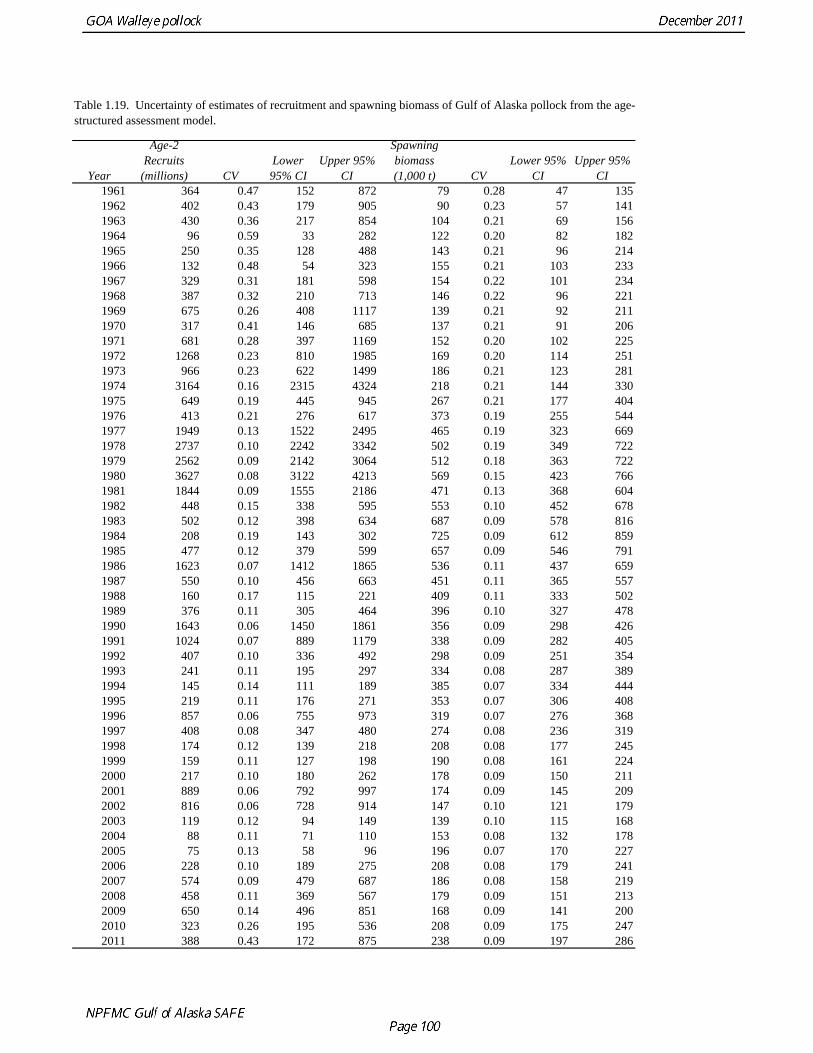
Year

Age-2 Recruits

(millions) CVLower 95% CI

Upper 95% CI

Spawning biomass (1,000 t) CV

Lower 95% CI

Upper 95% CI

1961 364 0.47 152 872 79 0.28 47 1351962 402 0.43 179 905 90 0.23 57 1411963 430 0.36 217 854 104 0.21 69 1561964 96 0.59 33 282 122 0.20 82 1821965 250 0.35 128 488 143 0.21 96 2141966 132 0.48 54 323 155 0.21 103 2331967 329 0.31 181 598 154 0.22 101 2341968 387 0.32 210 713 146 0.22 96 2211969 675 0.26 408 1117 139 0.21 92 2111970 317 0.41 146 685 137 0.21 91 2061971 681 0.28 397 1169 152 0.20 102 2251972 1268 0.23 810 1985 169 0.20 114 2511973 966 0.23 622 1499 186 0.21 123 2811974 3164 0.16 2315 4324 218 0.21 144 3301975 649 0.19 445 945 267 0.21 177 4041976 413 0.21 276 617 373 0.19 255 5441977 1949 0.13 1522 2495 465 0.19 323 6691978 2737 0.10 2242 3342 502 0.19 349 7221979 2562 0.09 2142 3064 512 0.18 363 7221980 3627 0.08 3122 4213 569 0.15 423 7661981 1844 0.09 1555 2186 471 0.13 368 6041982 448 0.15 338 595 553 0.10 452 6781983 502 0.12 398 634 687 0.09 578 8161984 208 0.19 143 302 725 0.09 612 8591985 477 0.12 379 599 657 0.09 546 7911986 1623 0.07 1412 1865 536 0.11 437 6591987 550 0.10 456 663 451 0.11 365 5571988 160 0.17 115 221 409 0.11 333 5021989 376 0.11 305 464 396 0.10 327 4781990 1643 0.06 1450 1861 356 0.09 298 4261991 1024 0.07 889 1179 338 0.09 282 4051992 407 0.10 336 492 298 0.09 251 3541993 241 0.11 195 297 334 0.08 287 3891994 145 0.14 111 189 385 0.07 334 4441995 219 0.11 176 271 353 0.07 306 4081996 857 0.06 755 973 319 0.07 276 3681997 408 0.08 347 480 274 0.08 236 3191998 174 0.12 139 218 208 0.08 177 2451999 159 0.11 127 198 190 0.08 161 2242000 217 0.10 180 262 178 0.09 150 2112001 889 0.06 792 997 174 0.09 145 2092002 816 0.06 728 914 147 0.10 121 1792003 119 0.12 94 149 139 0.10 115 1682004 88 0.11 71 110 153 0.08 132 1782005 75 0.13 58 96 196 0.07 170 2272006 228 0.10 189 275 208 0.08 179 2412007 574 0.09 479 687 186 0.08 158 2192008 458 0.11 369 567 179 0.09 151 2132009 650 0.14 496 851 168 0.09 141 2002010 323 0.26 195 536 208 0.09 175 2472011 388 0.43 172 875 238 0.09 197 286

Table 1.19. Uncertainty of estimates of recruitment and spawning biomass of Gulf of Alaska pollock from the age-structured assessment model.

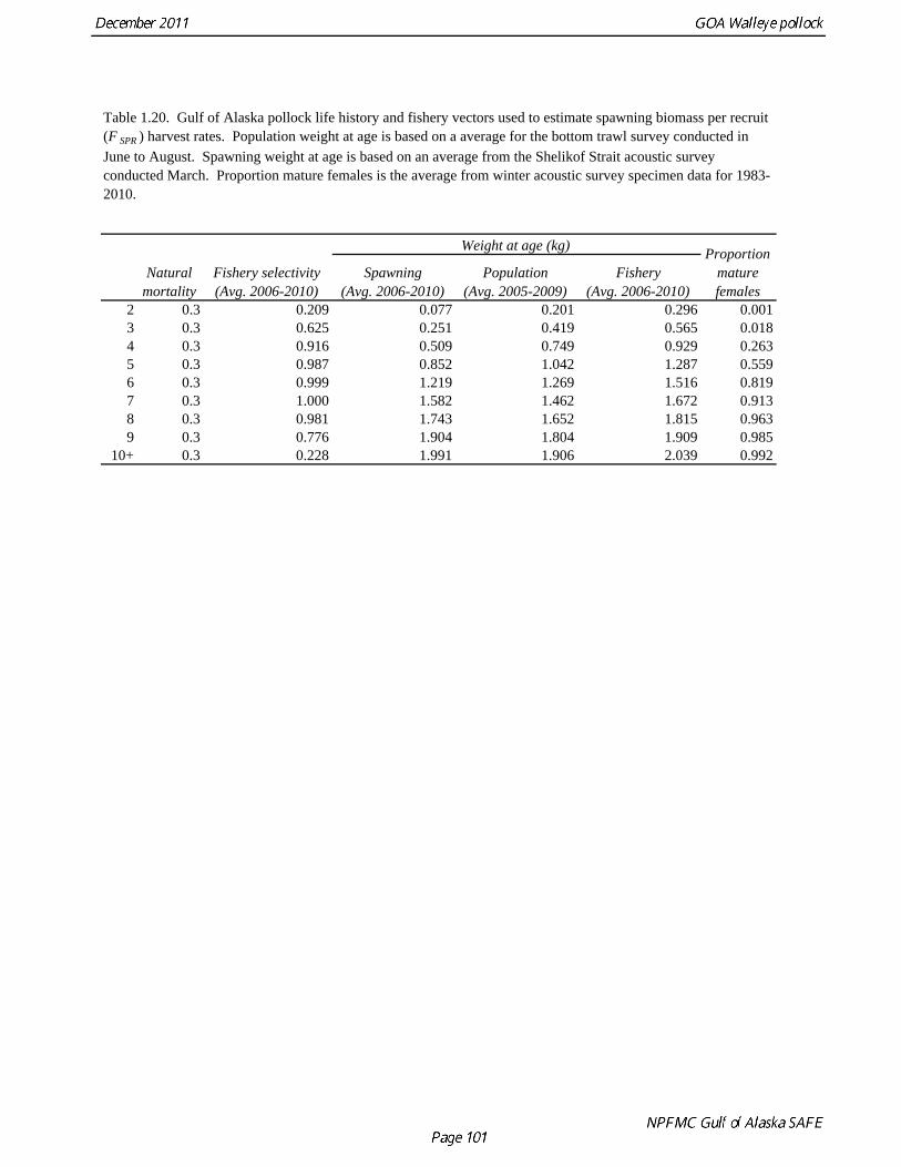
Natural mortality

Fishery selectivity (Avg. 2006-2010)

Weight at age (kg) Proportion mature females

Spawning (Avg. 2006-2010)

Population (Avg. 2005-2009)

Fishery (Avg. 2006-2010)

2 0.3 0.209 0.077 0.201 0.296 0.0013 0.3 0.625 0.251 0.419 0.565 0.0184 0.3 0.916 0.509 0.749 0.929 0.2635 0.3 0.987 0.852 1.042 1.287 0.5596 0.3 0.999 1.219 1.269 1.516 0.8197 0.3 1.000 1.582 1.462 1.672 0.9138 0.3 0.981 1.743 1.652 1.815 0.9639 0.3 0.776 1.904 1.804 1.909 0.985

10+ 0.3 0.228 1.991 1.906 2.039 0.992

Table 1.20. Gulf of Alaska pollock life history and fishery vectors used to estimate spawning biomass per recruit (F SPR ) harvest rates. Population weight at age is based on a average for the bottom trawl survey conducted in June to August. Spawning weight at age is based on an average from the Shelikof Strait acoustic survey conducted March. Proportion mature females is the average from winter acoustic survey specimen data for 1983-2010.

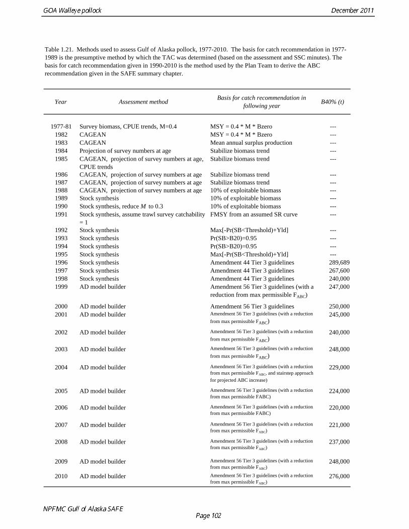
Year Assessment method Basis for catch recommendation in following year B40% (t)

1977-81 Survey biomass, CPUE trends, M=0.4 MSY = 0.4 * M * Bzero ---1982 CAGEAN MSY = 0.4 * M * Bzero ---1983 CAGEAN Mean annual surplus production ---1984 Projection of survey numbers at age Stabilize biomass trend ---1985 CAGEAN, projection of survey numbers at age,

CPUE trendsStabilize biomass trend ---

1986 CAGEAN, projection of survey numbers at age Stabilize biomass trend ---1987 CAGEAN, projection of survey numbers at age Stabilize biomass trend ---1988 CAGEAN, projection of survey numbers at age 10% of exploitable biomass ---1989 Stock synthesis 10% of exploitable biomass ---1990 Stock synthesis, reduce M to 0.3 10% of exploitable biomass ---1991 Stock synthesis, assume trawl survey catchability

= 1FMSY from an assumed SR curve ---

1992 Stock synthesis Max[-Pr(SB<Threshold)+Yld] ---1993 Stock synthesis Pr(SB>B20)=0.95 ---1994 Stock synthesis Pr(SB>B20)=0.95 ---1995 Stock synthesis Max[-Pr(SB<Threshold)+Yld] ---1996 Stock synthesis Amendment 44 Tier 3 guidelines 289,6891997 Stock synthesis Amendment 44 Tier 3 guidelines 267,6001998 Stock synthesis Amendment 44 Tier 3 guidelines 240,0001999 AD model builder Amendment 56 Tier 3 guidelines (with a

reduction from max permissible FABC)247,000

2000 AD model builder Amendment 56 Tier 3 guidelines 250,0002001 AD model builder Amendment 56 Tier 3 guidelines (with a reduction

from max permissible FABC)245,000

2002 AD model builder Amendment 56 Tier 3 guidelines (with a reduction from max permissible FABC)

240,000

2003 AD model builder Amendment 56 Tier 3 guidelines (with a reduction from max permissible FABC)

248,000

2004 AD model builder Amendment 56 Tier 3 guidelines (with a reduction from max permissible FABC, and stairstep approach for projected ABC increase)

229,000

2005 AD model builder Amendment 56 Tier 3 guidelines (with a reduction from max permissible FABC)

224,000

2006 AD model builder Amendment 56 Tier 3 guidelines (with a reduction from max permissible FABC)

220,000

2007 AD model builder Amendment 56 Tier 3 guidelines (with a reduction from max permissible FABC)

221,000

2008 AD model builder Amendment 56 Tier 3 guidelines (with a reduction from max permissible FABC)

237,000

2009 AD model builder Amendment 56 Tier 3 guidelines (with a reduction from max permissible FABC)

248,000

2010 AD model builder Amendment 56 Tier 3 guidelines (with a reduction from max permissible FABC)

276,000

Table 1.21. Methods used to assess Gulf of Alaska pollock, 1977-2010. The basis for catch recommendation in 1977-1989 is the presumptive method by which the TAC was determined (based on the assessment and SSC minutes). The basis for catch recommendation given in 1990-2010 is the method used by the Plan Team to derive the ABC recommendation given in the SAFE summary chapter.

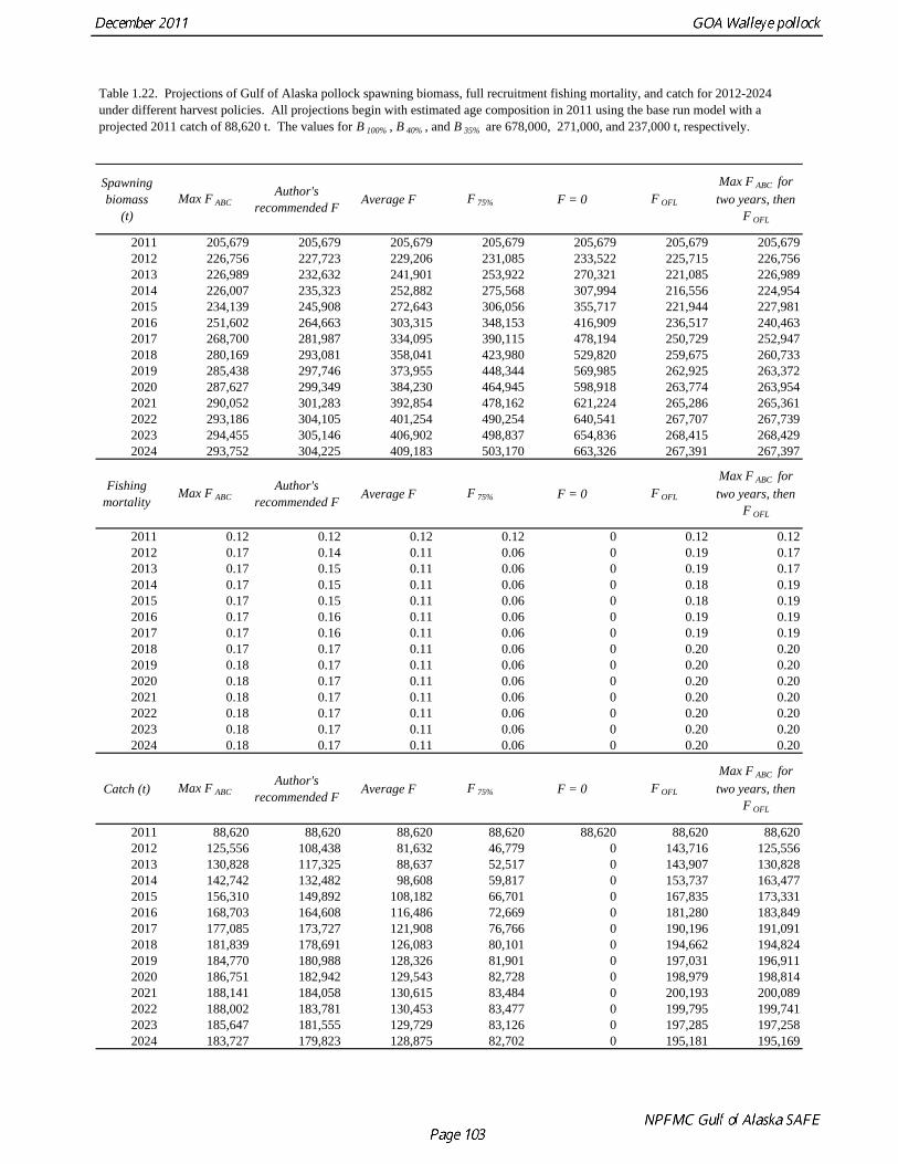
Spawning biomass

(t)Max F ABC

Author's recommended F Average F F 75% F = 0 F OFL

Max F ABC for two years, then

F OFL

2011 205,679 205,679 205,679 205,679 205,679 205,679 205,6792012 226,756 227,723 229,206 231,085 233,522 225,715 226,7562013 226,989 232,632 241,901 253,922 270,321 221,085 226,9892014 226,007 235,323 252,882 275,568 307,994 216,556 224,9542015 234,139 245,908 272,643 306,056 355,717 221,944 227,9812016 251,602 264,663 303,315 348,153 416,909 236,517 240,4632017 268,700 281,987 334,095 390,115 478,194 250,729 252,9472018 280,169 293,081 358,041 423,980 529,820 259,675 260,7332019 285,438 297,746 373,955 448,344 569,985 262,925 263,3722020 287,627 299,349 384,230 464,945 598,918 263,774 263,9542021 290,052 301,283 392,854 478,162 621,224 265,286 265,3612022 293,186 304,105 401,254 490,254 640,541 267,707 267,7392023 294,455 305,146 406,902 498,837 654,836 268,415 268,4292024 293,752 304,225 409,183 503,170 663,326 267,391 267,397

Fishing mortality

Max F ABCAuthor's

recommended F Average F F 75% F = 0 F OFL

Max F ABC for two years, then

F OFL

2011 0.12 0.12 0.12 0.12 0 0.12 0.122012 0.17 0.14 0.11 0.06 0 0.19 0.172013 0.17 0.15 0.11 0.06 0 0.19 0.172014 0.17 0.15 0.11 0.06 0 0.18 0.192015 0.17 0.15 0.11 0.06 0 0.18 0.192016 0.17 0.16 0.11 0.06 0 0.19 0.192017 0.17 0.16 0.11 0.06 0 0.19 0.192018 0.17 0.17 0.11 0.06 0 0.20 0.202019 0.18 0.17 0.11 0.06 0 0.20 0.202020 0.18 0.17 0.11 0.06 0 0.20 0.202021 0.18 0.17 0.11 0.06 0 0.20 0.202022 0.18 0.17 0.11 0.06 0 0.20 0.202023 0.18 0.17 0.11 0.06 0 0.20 0.202024 0.18 0.17 0.11 0.06 0 0.20 0.20

Catch (t) Max F ABCAuthor's

recommended F Average F F 75% F = 0 F OFL

Max F ABC for two years, then

F OFL

2011 88,620 88,620 88,620 88,620 88,620 88,620 88,6202012 125,556 108,438 81,632 46,779 0 143,716 125,5562013 130,828 117,325 88,637 52,517 0 143,907 130,8282014 142,742 132,482 98,608 59,817 0 153,737 163,4772015 156,310 149,892 108,182 66,701 0 167,835 173,3312016 168,703 164,608 116,486 72,669 0 181,280 183,8492017 177,085 173,727 121,908 76,766 0 190,196 191,0912018 181,839 178,691 126,083 80,101 0 194,662 194,8242019 184,770 180,988 128,326 81,901 0 197,031 196,9112020 186,751 182,942 129,543 82,728 0 198,979 198,8142021 188,141 184,058 130,615 83,484 0 200,193 200,0892022 188,002 183,781 130,453 83,477 0 199,795 199,7412023 185,647 181,555 129,729 83,126 0 197,285 197,2582024 183,727 179,823 128,875 82,702 0 195,181 195,169

Table 1.22. Projections of Gulf of Alaska pollock spawning biomass, full recruitment fishing mortality, and catch for 2012-2024 under different harvest policies. All projections begin with estimated age composition in 2011 using the base run model with a projected 2011 catch of 88,620 t. The values for B 100% , B 40% , and B 35% are 678,000, 271,000, and 237,000 t, respectively.

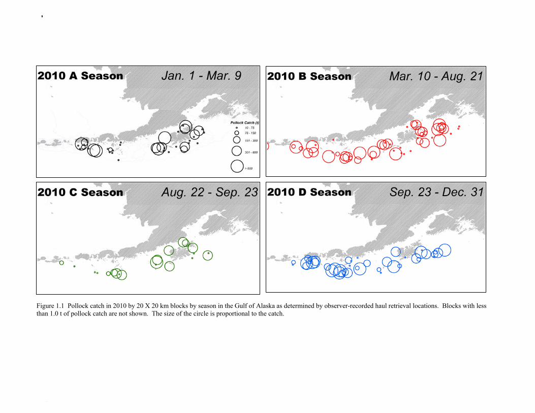
Figure 1.1 Pollock catch in 2010 by 20 X 20 km blocks by season in the Gulf of Alaska as determined by observer-recorded haul retrieval locations. Blocks with less than 1.0 t of pollock catch are not shown. The size of the circle is proportional to the catch.

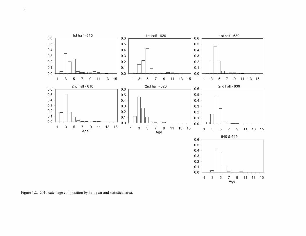
1st half - 610

0.0

0.10.2

0.3

0.40.5

0.6

1 3 5 7 9 11 13 15

1st half - 620

0.0

0.10.2

0.30.4

0.50.6

1 3 5 7 9 11 13 15

1st half - 630

0.0

0.10.2

0.30.4

0.50.6

1 3 5 7 9 11 13 15

2nd half - 610

0.00.10.20.30.40.50.6

1 3 5 7 9 11 13 15Age

2nd half - 620

0.00.10.20.30.40.50.6

1 3 5 7 9 11 13 15Age

2nd half - 630

0.00.1

0.20.30.4

0.50.6

1 3 5 7 9 11 13 15

640 & 649

0.00.10.20.30.40.50.6

1 3 5 7 9 11 13 15Age

Figure 1.2. 2010 catch age composition by half year and statistical area.

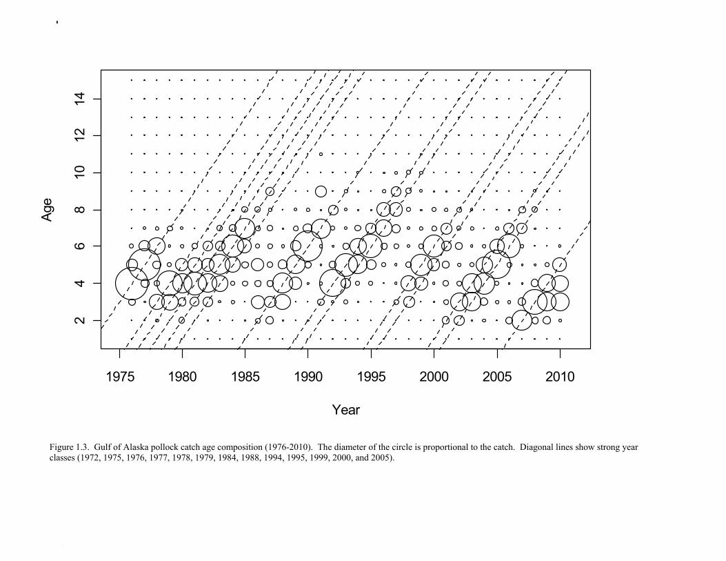
1975 1980 1985 1990 1995 2000 2005 2010

24

68

1012

14

Year

Age

Figure 1.3. Gulf of Alaska pollock catch age composition (1976-2010). The diameter of the circle is proportional to the catch. Diagonal lines show strong year classes (1972, 1975, 1976, 1977, 1978, 1979, 1984, 1988, 1994, 1995, 1999, 2000, and 2005).

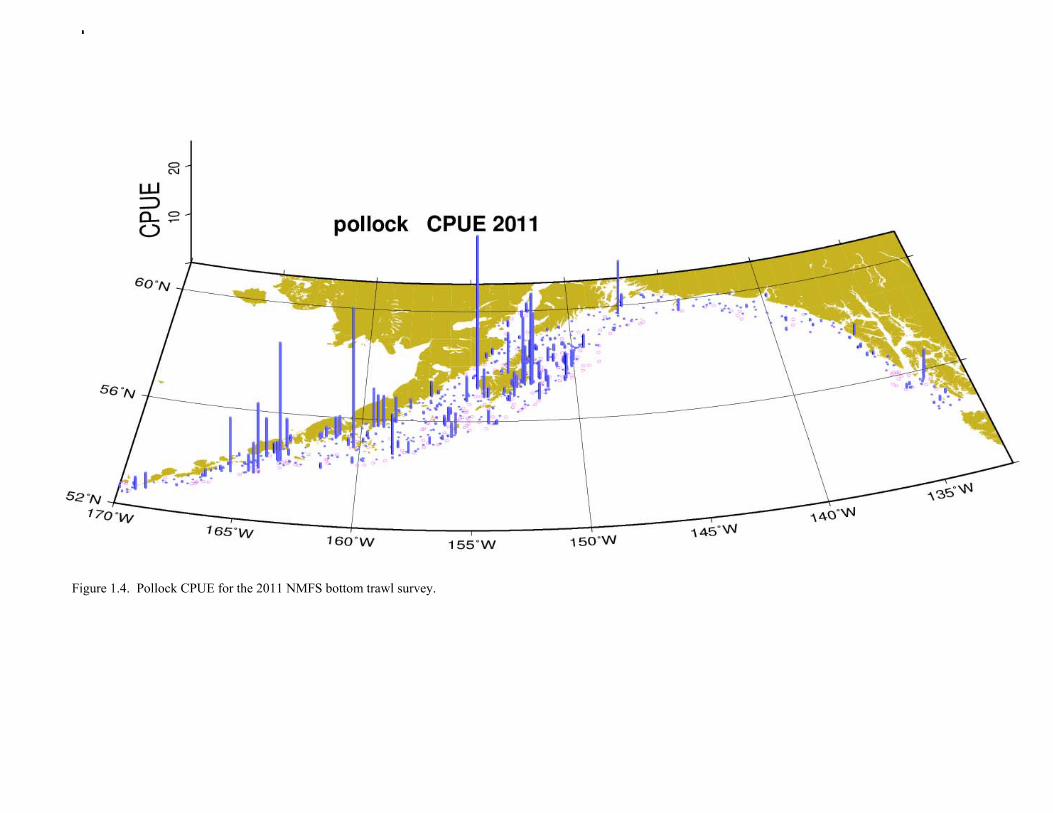
Figure 1.4. Pollock CPUE for the 2011 NMFS bottom trawl survey.

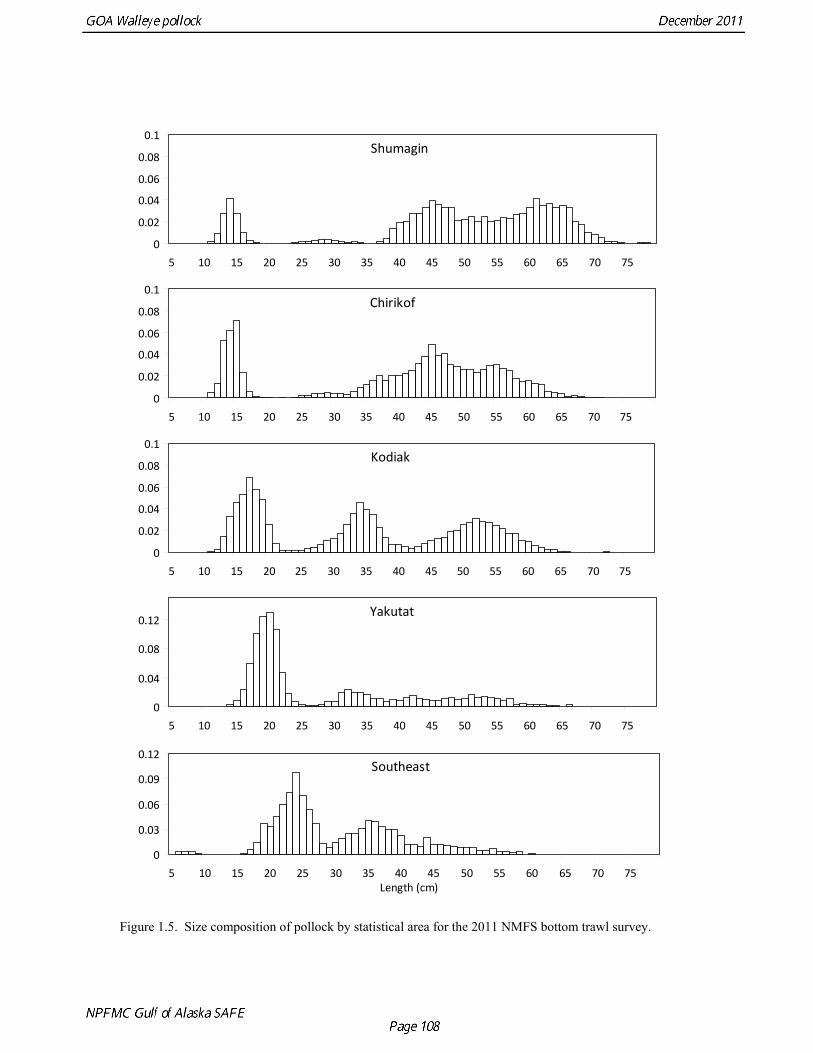
Shumagin

0

0.02

0.04

0.06

0.08

0.1

5 10 15 20 25 30 35 40 45 50 55 60 65 70 75

Chirikof

0

0.02

0.04

0.06

0.08

0.1

5 10 15 20 25 30 35 40 45 50 55 60 65 70 75

Kodiak

0

0.02

0.04

0.06

0.08

0.1

5 10 15 20 25 30 35 40 45 50 55 60 65 70 75

Yakutat

0

0.04

0.08

0.12

5 10 15 20 25 30 35 40 45 50 55 60 65 70 75

Southeast

0

0.03

0.06

0.09

0.12

5 10 15 20 25 30 35 40 45 50 55 60 65 70 75Length (cm)

Figure 1.5. Size composition of pollock by statistical area for the 2011 NMFS bottom trawl survey.

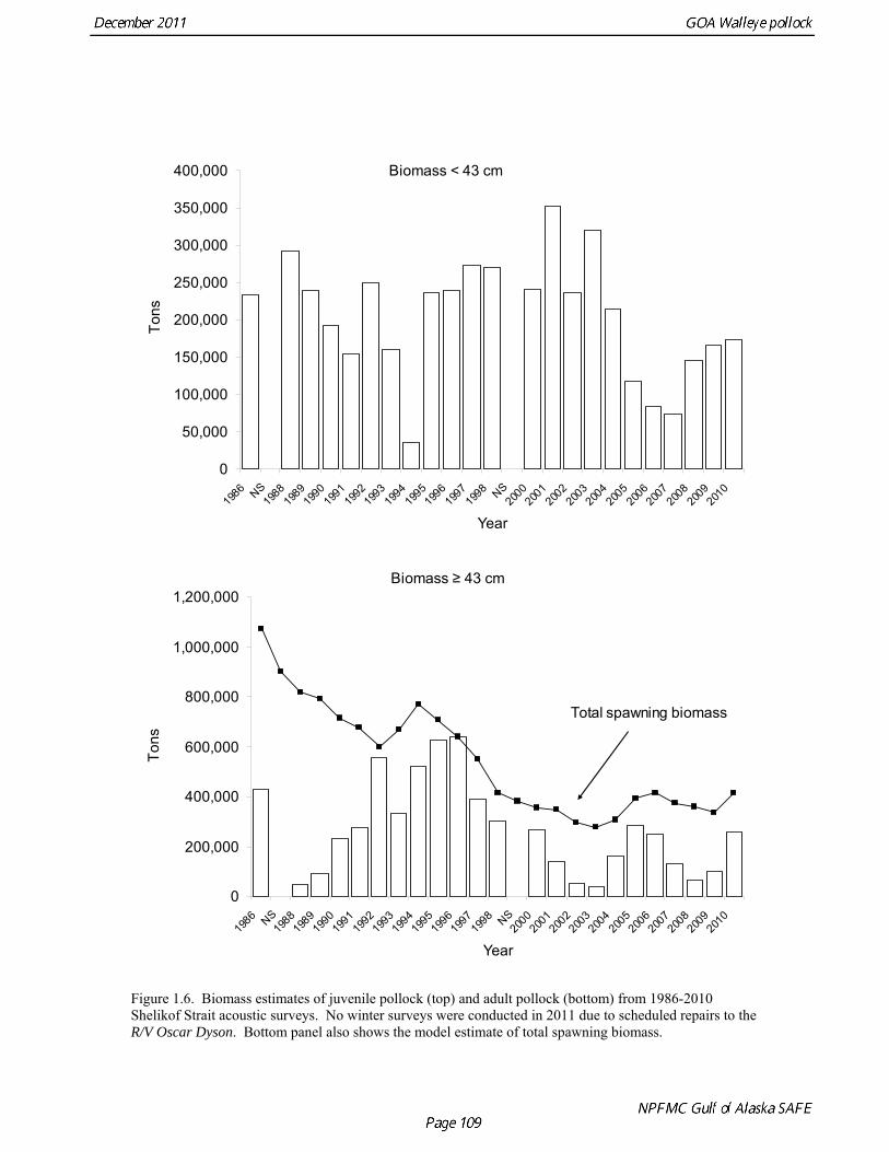
Biomass < 43 cm

0

50,000

100,000

150,000

200,000

250,000

300,000

350,000

400,000

1986 NS

1988

1989

1990

1991

1992

1993

1994

1995

1996

1997

1998 NS

2000

2001

2002

2003

2004

2005

2006

2007

2008

2009

2010

Year

Tons

0

200,000

400,000

600,000

800,000

1,000,000

1,200,000

1986 NS

1988

1989

1990

1991

1992

1993

1994

1995

1996

1997

1998 NS

2000

2001

2002

2003

2004

2005

2006

2007

2008

2009

2010

Year

Tons

Total spawning biomass

Biomass ≥ 43 cm

Figure 1.6. Biomass estimates of juvenile pollock (top) and adult pollock (bottom) from 1986-2010 Shelikof Strait acoustic surveys. No winter surveys were conducted in 2011 due to scheduled repairs to the R/V Oscar Dyson. Bottom panel also shows the model estimate of total spawning biomass.

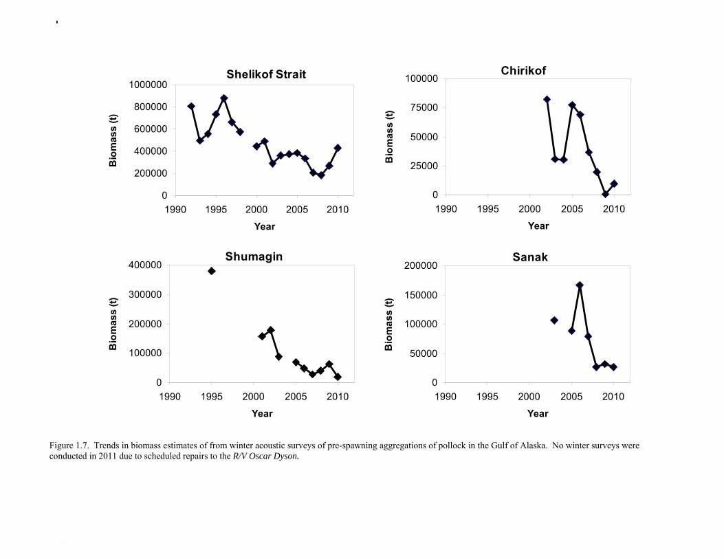
Chirikof100000

0

25000

50000

75000

1990 1995 2000 2005 2010

Year

Bio

mas

s (t)

Shelikof Strait

0

200000

400000

600000

800000

1000000

1990 1995 2000 2005 2010

Year

Bio

mas

s (t)

Shumagin

0

100000

200000

300000

400000

1990 1995 2000 2005 2010

Year

Bio

mas

s (t)

Sanak

0

50000

100000

150000

200000

1990 1995 2000 2005 2010

Year

Bio

mas

s (t)

Figure 1.7. Trends in biomass estimates of from winter acoustic surveys of pre-spawning aggregations of pollock in the Gulf of Alaska. No winter surveys were conducted in 2011 due to scheduled repairs to the R/V Oscar Dyson.

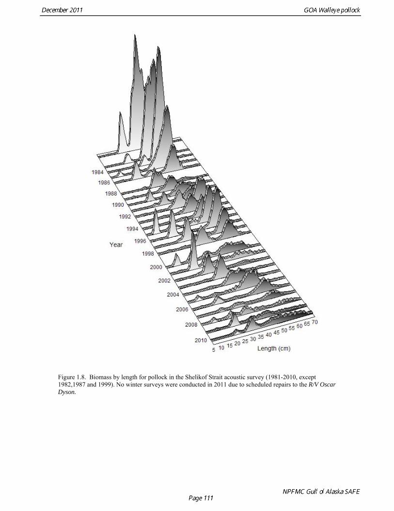
Figure 1.8. Biomass by length for pollock in the Shelikof Strait acoustic survey (1981-2010, except 1982,1987 and 1999). No winter surveys were conducted in 2011 due to scheduled repairs to the R/V Oscar Dyson.

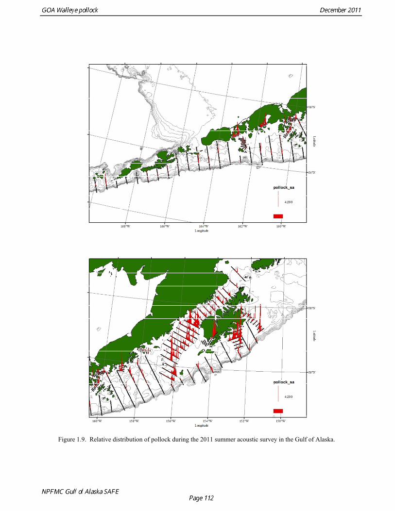
Figure 1.9. Relative distribution of pollock during the 2011 summer acoustic survey in the Gulf of Alaska.

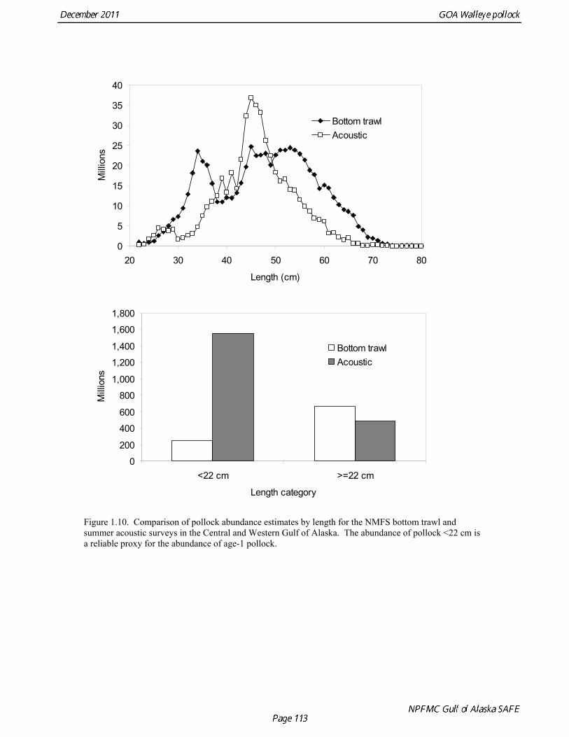
0

5

10

15

20

25

30

35

40

20 30 40 50 60 70 80

Length (cm)

Mill

ions

Bottom trawlAcoustic

0

200

400

600

800

1,000

1,200

1,400

1,600

1,800

<22 cm >=22 cm

Length category

Mill

ions

Bottom trawlAcoustic

Figure 1.10. Comparison of pollock abundance estimates by length for the NMFS bottom trawl and summer acoustic surveys in the Central and Western Gulf of Alaska. The abundance of pollock <22 cm is a reliable proxy for the abundance of age-1 pollock.

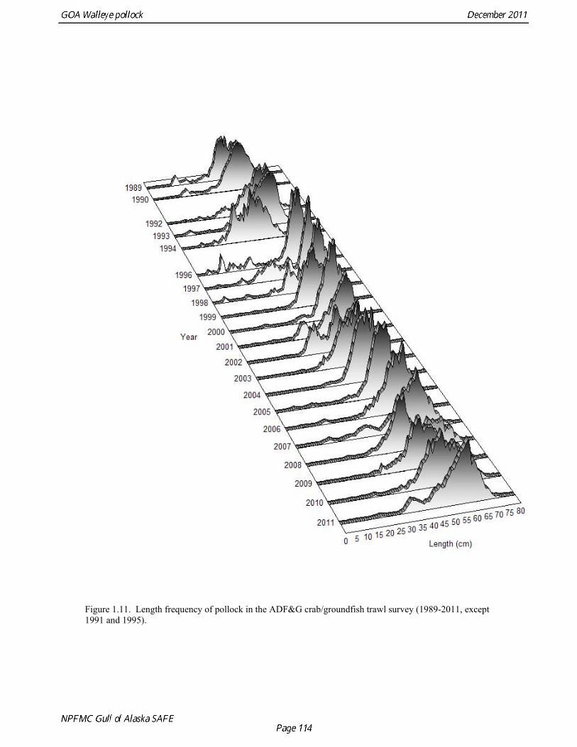
Figure 1.11. Length frequency of pollock in the ADF&G crab/groundfish trawl survey (1989-2011, except 1991 and 1995).

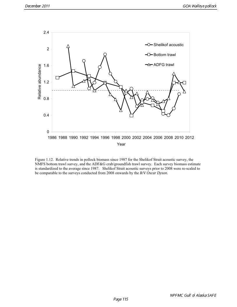
0

0.4

0.8

1.2

1.6

2

2.4

1986 1988 1990 1992 1994 1996 1998 2000 2002 2004 2006 2008 2010 2012

Year

Rel

ativ

e ab

unda

nce

Shelikof acoustic

Bottom trawl

ADFG trawl

Figure 1.12. Relative trends in pollock biomass since 1987 for the Shelikof Strait acoustic survey, the NMFS bottom trawl survey, and the ADF&G crab/groundfish trawl survey. Each survey biomass estimate is standardized to the average since 1987. Shelikof Strait acoustic surveys prior to 2008 were re-scaled to be comparable to the surveys conducted from 2008 onwards by the R/V Oscar Dyson.

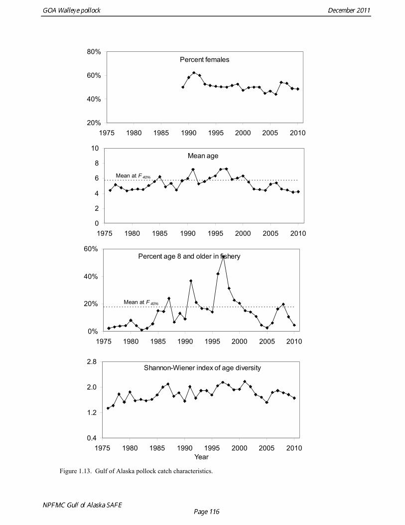
Percent females

20%

40%

60%

80%

1975 1980 1985 1990 1995 2000 2005 2010

Mean age

0

2

4

6

8

10

1975 1980 1985 1990 1995 2000 2005 2010

Mean at F 40%

Percent age 8 and older in fishery

0%

20%

40%

60%

1975 1980 1985 1990 1995 2000 2005 2010

Mean at F 40%

Shannon-Wiener index of age diversity

0.4

1.2

2.0

2.8

1975 1980 1985 1990 1995 2000 2005 2010Year

Figure 1.13. Gulf of Alaska pollock catch characteristics.

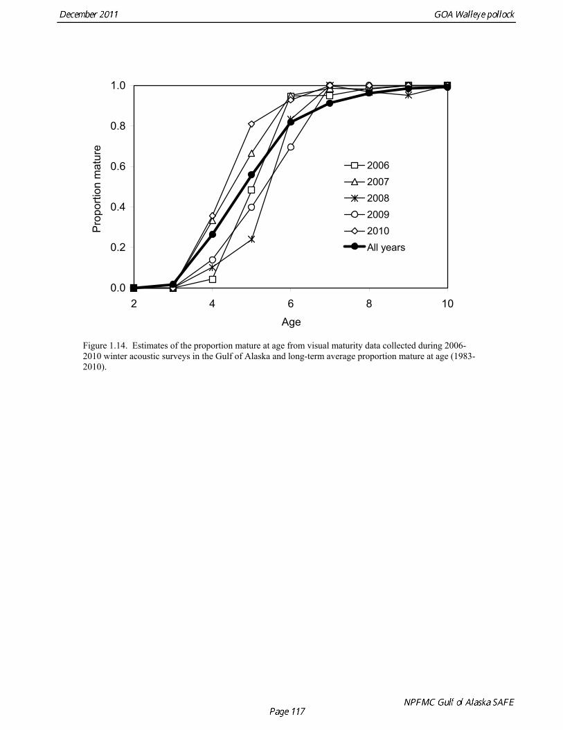
0.0

0.2

0.4

0.6

0.8

1.0

2 4 6 8 1

Age

Pro

porti

on m

atur

e

0

20062007200820092010All years

Figure 1.14. Estimates of the proportion mature at age from visual maturity data collected during 2006-2010 winter acoustic surveys in the Gulf of Alaska and long-term average proportion mature at age (1983-2010).

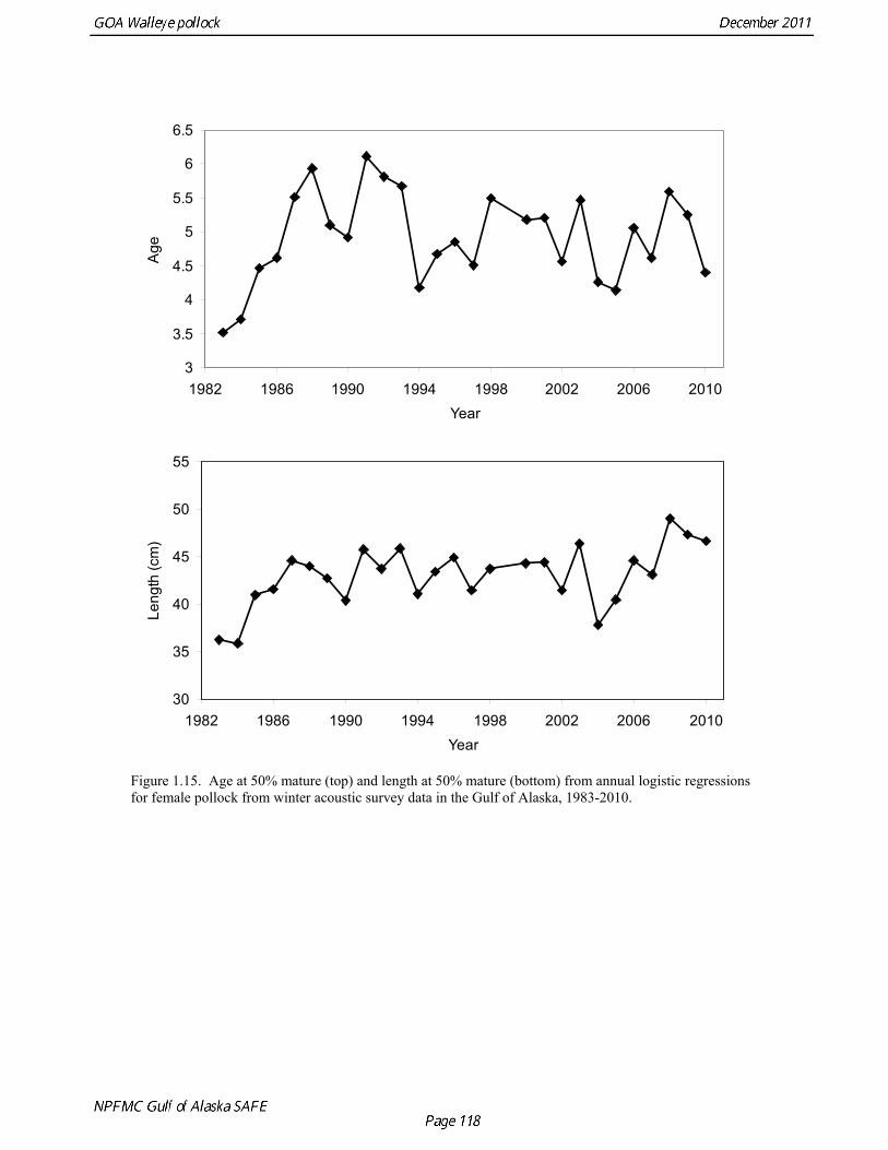
3

3.5

4

4.5

5

5.5

6

6.5

1982 1986 1990 1994 1998 2002 2006 2010Year

Age

30

35

40

45

50

55

1982 1986 1990 1994 1998 2002 2006 2010Year

Leng

th (c

m)

Figure 1.15. Age at 50% mature (top) and length at 50% mature (bottom) from annual logistic regressions for female pollock from winter acoustic survey data in the Gulf of Alaska, 1983-2010.

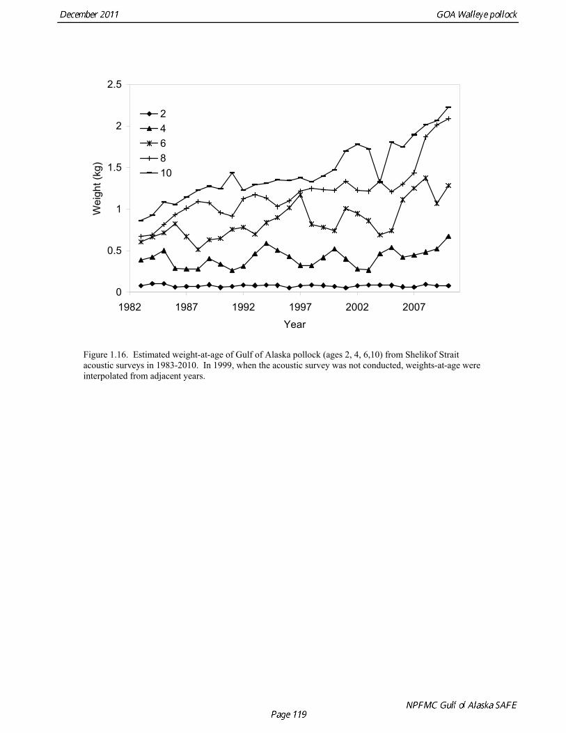
0

0.5

1

1.5

2

2.5

1982 1987 1992 1997 2002 2007

Year

Wei

ght (

kg)

246810

Figure 1.16. Estimated weight-at-age of Gulf of Alaska pollock (ages 2, 4, 6,10) from Shelikof Strait acoustic surveys in 1983-2010. In 1999, when the acoustic survey was not conducted, weights-at-age were interpolated from adjacent years.

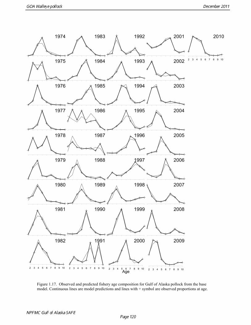
1974 1983 1992 2001 2010

1975 1984 1993 2002

1976 1985 1994 2003

1977 1986 1995 2004

1978 1987 1996 2005

1979 1988 1997 2006

1980 1989 1998 2007

1981 1990 1999 2008

1982 1991 2000 2009

Age2 3 4 5 6 7 8 9 10 2 3 4 5 6 7 8 9 102 3 4 5 6 7 8 9 10 2 3 4 5 6 7 8 9 10

2 3 4 5 6 7 8 9 10

Figure 1.17. Observed and predicted fishery age composition for Gulf of Alaska pollock from the base model. Continuous lines are model predictions and lines with + symbol are observed proportions at age.

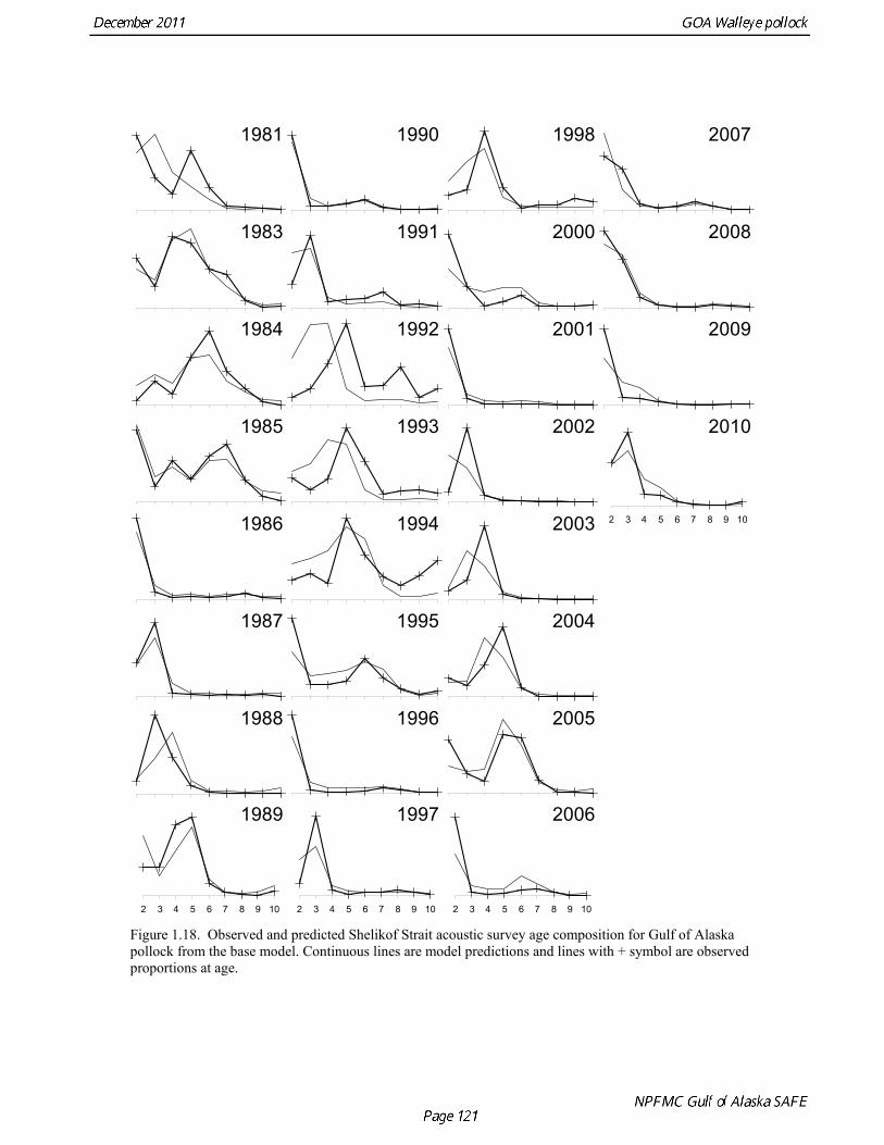
1981 1990 1998 2007

1983 1991 2000 2008

1984 1992 2001 2009

1985 1993 2002 2010

1986 1994 2003

1987 1995 2004

1988 1996 2005

1989 1997 2006

2 3 4 5 6 7 8 9 102 3 4 5 6 7 8 9 102 3 4 5 6 7 8 9 10

2 3 4 5 6 7 8 9 10

Figure 1.18. Observed and predicted Shelikof Strait acoustic survey age composition for Gulf of Alaska pollock from the base model. Continuous lines are model predictions and lines with + symbol are observed proportions at age.

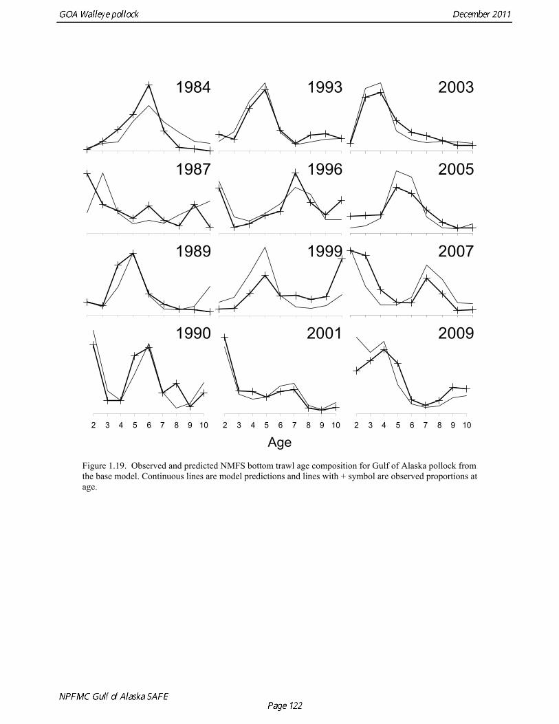
1984 1993 2003

1987 1996 2005

1989 1999 2007

1990 2001 2009

Age2 3 4 5 6 7 8 9 10 2 3 4 5 6 7 8 9 10 2 3 4 5 6 7 8 9 10

Figure 1.19. Observed and predicted NMFS bottom trawl age composition for Gulf of Alaska pollock from the base model. Continuous lines are model predictions and lines with + symbol are observed proportions at age.

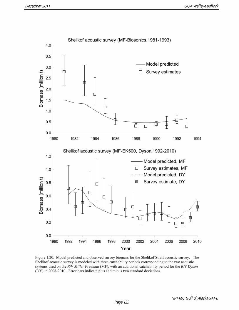
Shelikof acoustic survey (MF-Biosonics,1981-1993)

0.0

0.5

1.0

1.5

2.0

2.5

3.0

3.5

4.0

1980 1982 1984 1986 1988 1990 1992 1994

Biom

ass

(milli

on t)

Model predicted

Survey estimates

Shelikof acoustic survey (MF-EK500, Dyson,1992-2010)

0.0

0.2

0.4

0.6

0.8

1.0

1.2

1990 1992 1994 1996 1998 2000 2002 2004 2006 2008 2010

Year

Biom

ass

(milli

on t)

Model predicted, MFSurvey estimates, MFModel predicted, DYSurvey estimate, DY

Figure 1.20. Model predicted and observed survey biomass for the Shelikof Strait acoustic survey. The Shelikof acoustic survey is modeled with three catchability periods corresponding to the two acoustic systems used on the R/V Miller Freeman (MF), with an additional catchability period for the R/V Dyson (DY) in 2008-2010. Error bars indicate plus and minus two standard deviations.

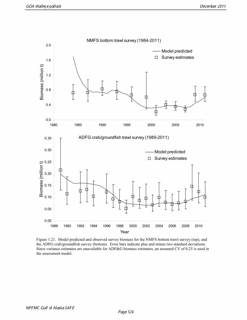
NMFS bottom trawl survey (1984-2011)

0.0

0.4

0.8

1.2

1.6

2.0

1980 1985 1990 1995 2000 2005 2010

Bio

mas

s (m

illio

n t)

Model predictedSurvey estimates

ADFG crab/groundfish trawl survey (1989-2011)

0.00

0.05

0.10

0.15

0.20

0.25

0.30

0.35

1988 1990 1992 1994 1996 1998 2000 2002 2004 2006 2008 2010

Year

Bio

mas

s (m

illio

n t)

Model predictedSurvey estimates

Figure 1.21. Model predicted and observed survey biomass for the NMFS bottom trawl survey (top), and the ADFG crab/groundfish survey (bottom). Error bars indicate plus and minus two standard deviations. Since variance estimates are unavailable for ADF&G biomass estimates, an assumed CV of 0.25 is used in the assessment model.

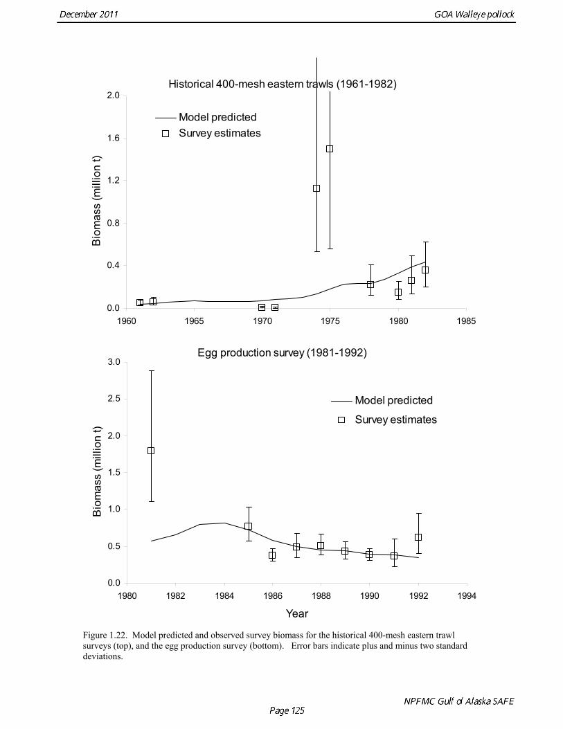
Historical 400-mesh eastern trawls (1961-1982)

0.0

0.4

0.8

1.2

1.6

2.0

1960 1965 1970 1975 1980 1985

Bio

mas

s (m

illio

n t)

Model predictedSurvey estimates

Egg production survey (1981-1992)

0.0

0.5

1.0

1.5

2.0

2.5

3.0

1980 1982 1984 1986 1988 1990 1992 1994

Year

Bio

mas

s (m

illio

n t)

Model predicted

Survey estimates

Figure 1.22. Model predicted and observed survey biomass for the historical 400-mesh eastern trawl surveys (top), and the egg production survey (bottom). Error bars indicate plus and minus two standard deviations.

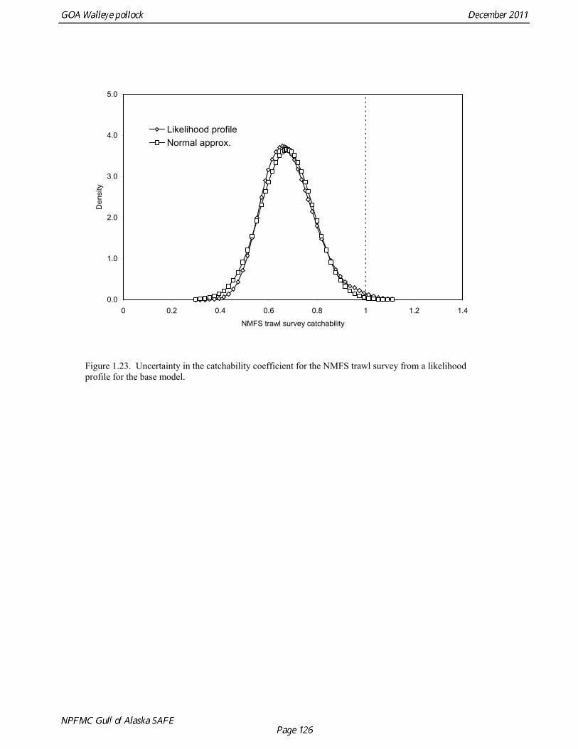
0.0

1.0

2.0

3.0

4.0

5.0

0 0.2 0.4 0.6 0.8 1 1.2 1.4

NMFS trawl survey catchability

Den

sity

Likelihood profileNormal approx.

Figure 1.23. Uncertainty in the catchability coefficient for the NMFS trawl survey from a likelihood profile for the base model.

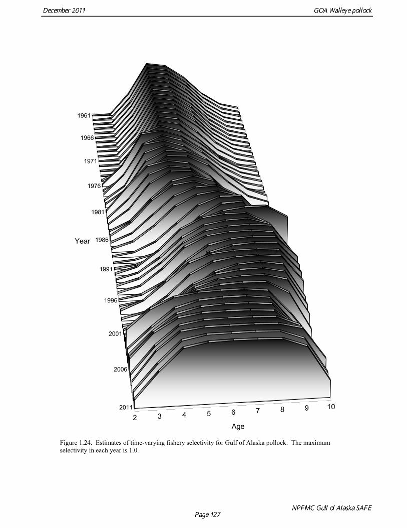
2 3 4 5 6 7 8 9 102011

2006

2001

1996

1991

1986

1981

1976

1971

1966

1961

Age

Yeary

Figure 1.24. Estimates of time-varying fishery selectivity for Gulf of Alaska pollock. The maximum selectivity in each year is 1.0.

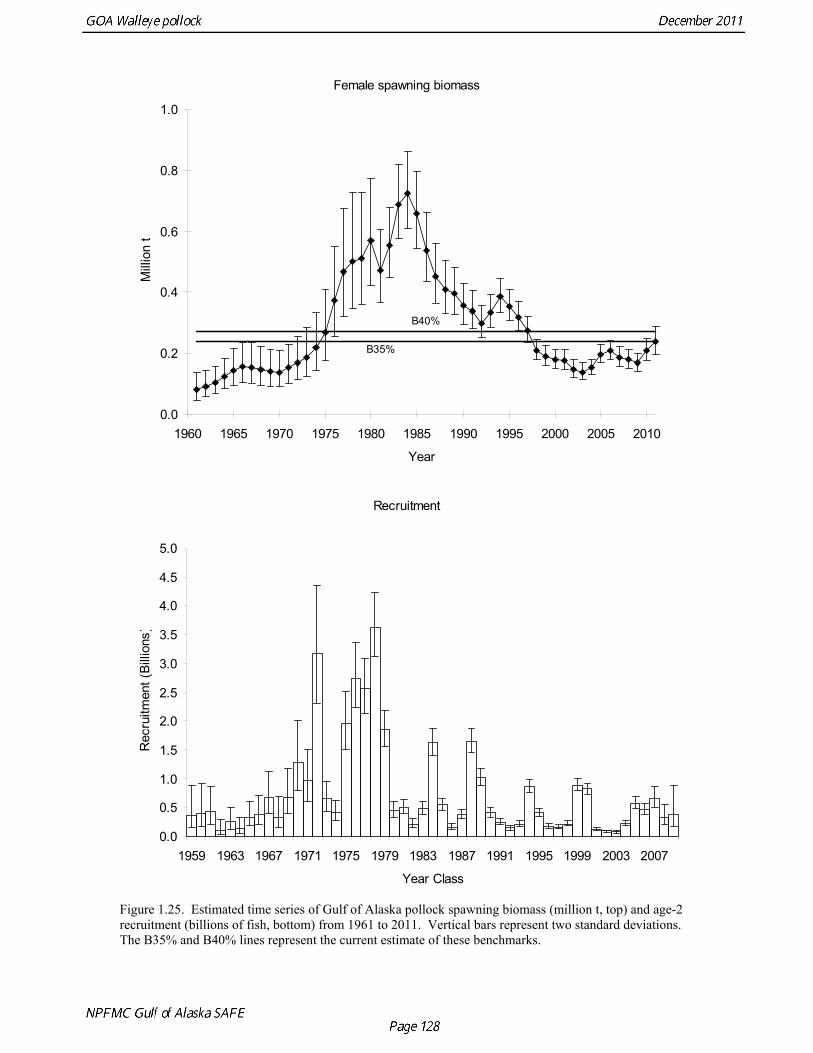
Female spawning biomass

0.0

0.2

0.4

0.6

0.8

1.0

1960 1965 1970 1975 1980 1985 1990 1995 2000 2005 2010

Year

Mill

ion

t

B40%

B35%

Recruitment

0.0

0.5

1.0

1.5

2.0

2.5

3.0

3.5

4.0

4.5

5.0

1959 1963 1967 1971 1975 1979 1983 1987 1991 1995 1999 2003 2007

Year Class

Rec

ruitm

ent (

Billi

ons)

Figure 1.25. Estimated time series of Gulf of Alaska pollock spawning biomass (million t, top) and age-2 recruitment (billions of fish, bottom) from 1961 to 2011. Vertical bars represent two standard deviations. The B35% and B40% lines represent the current estimate of these benchmarks.

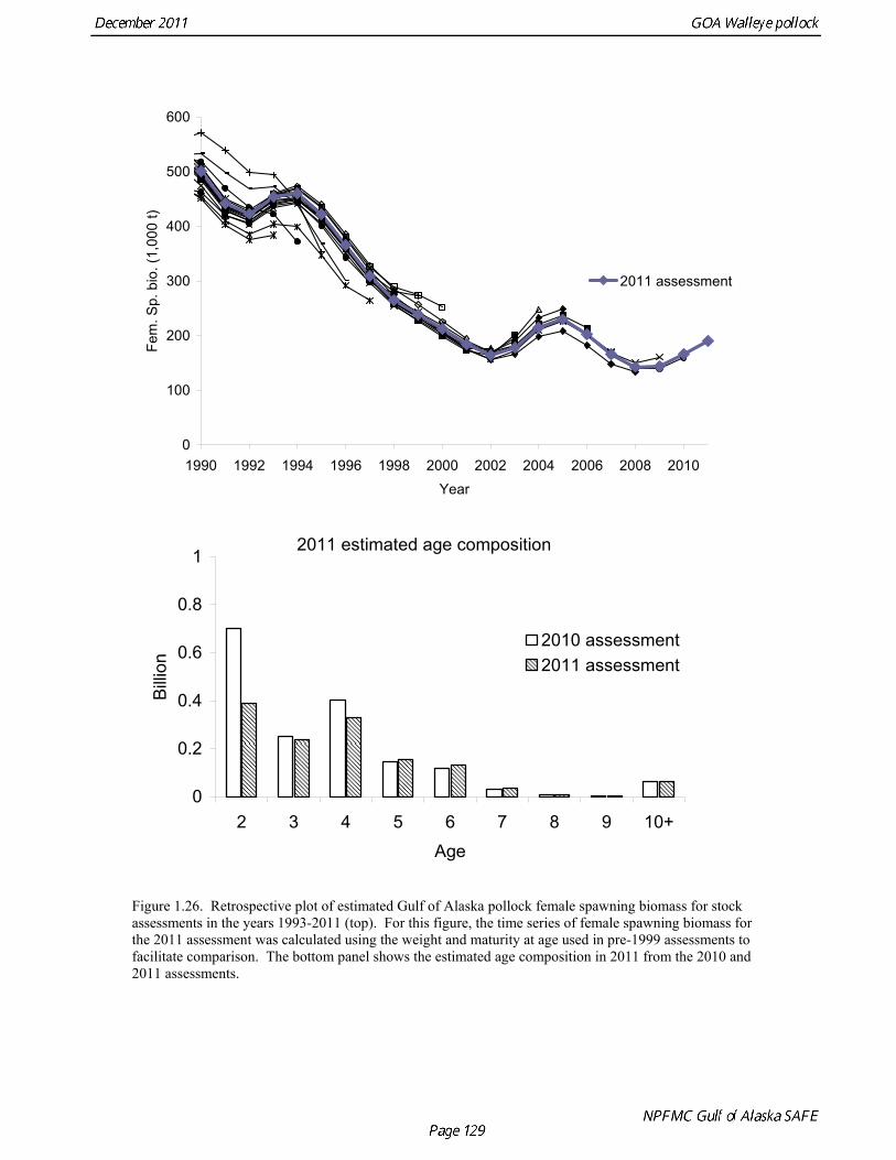
0

100

200

300

400

500

600

1990 1992 1994 1996 1998 2000 2002 2004 2006 2008 2010

Year

Fem

. Sp.

bio

. (1,

000

t)

2011 assessment

2011 estimated age composition

0

0.2

0.4

0.6

0.8

1

2 3 4 5 6 7 8 9 10+

Age

Billio

n

2010 assessment2011 assessment

Figure 1.26. Retrospective plot of estimated Gulf of Alaska pollock female spawning biomass for stock assessments in the years 1993-2011 (top). For this figure, the time series of female spawning biomass for the 2011 assessment was calculated using the weight and maturity at age used in pre-1999 assessments to facilitate comparison. The bottom panel shows the estimated age composition in 2011 from the 2010 and 2011 assessments.

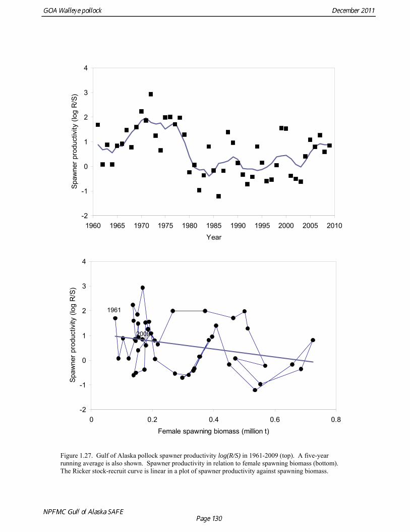
-2

-1

0

1

2

3

4

1960 1965 1970 1975 1980 1985 1990 1995 2000 2005 2010Year

Spaw

ner p

rodu

ctiv

ity (l

og R

/S)

-2

-1

0

1

2

3

4

0 0.2 0.4 0.6 0.8Female spawning biomass (million t)

Spaw

ner p

rodu

ctiv

ity (l

og R

/S)

1961

2009

Figure 1.27. Gulf of Alaska pollock spawner productivity log(R/S) in 1961-2009 (top). A five-year running average is also shown. Spawner productivity in relation to female spawning biomass (bottom). The Ricker stock-recruit curve is linear in a plot of spawner productivity against spawning biomass.

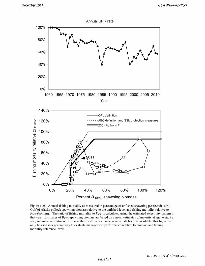
Annual SPR rate

0%

20%

40%

60%

80%

100%

1960 1965 1970 1975 1980 1985 1990 1995 2000 2005 2010Year

0%

20%

40%

60%

80%

100%

120%

140%

0% 20% 40% 60% 80% 100% 120%

Percent B 100% spawning biomass

Fish

ing

mor

talit

y re

lativ

e to

FM

SY

OFL definitionABC definition and SSL protection measures 2001 Author's F

2011

Figure 1.28. Annual fishing mortality as measured in percentage of unfished spawning per recruit (top). Gulf of Alaska pollock spawning biomass relative to the unfished level and fishing mortality relative to FMSY (bottom). The ratio of fishing mortality to FMSY is calculated using the estimated selectivity pattern in that year. Estimates of B100% spawning biomass are based on current estimates of maturity at age, weight at age, and mean recruitment. Because these estimates change as new data become available, this figure can only be used in a general way to evaluate management performance relative to biomass and fishing mortality reference levels.

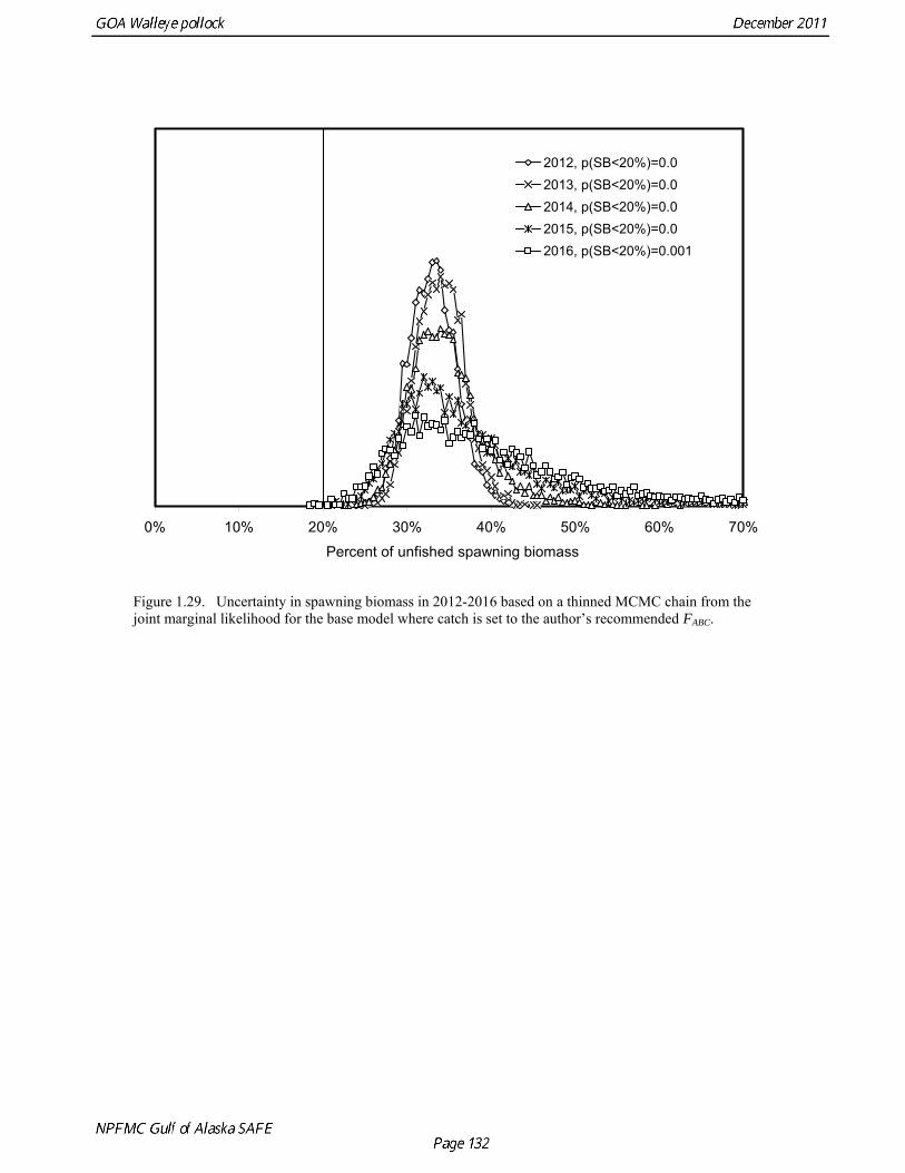
0% 10% 20% 30% 40% 50% 60% 70%

Percent of unfished spawning biomass

2012, p(SB<20%)=0.02013, p(SB<20%)=0.02014, p(SB<20%)=0.02015, p(SB<20%)=0.02016, p(SB<20%)=0.001

Figure 1.29. Uncertainty in spawning biomass in 2012-2016 based on a thinned MCMC chain from the joint marginal likelihood for the base model where catch is set to the author’s recommended FABC.

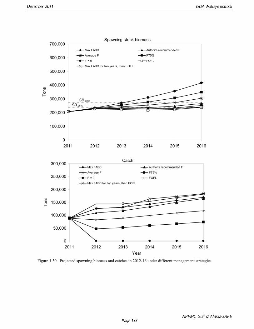
Spawning stock biomass

0

100,000

200,000

300,000

400,000

500,000

600,000

700,000

2011 2012 2013 2014 2015 2016

Tons

Max FABC Author's recommended F

Average F F75%

F = 0 FOFL

Max FABC for two years, then FOFL

SB 40%

SB 35%

Catch

0

50,000

100,000

150,000

200,000

250,000

300,000

2011 2012 2013 2014 2015 2016Year

Tons

Max FABC Author's recommended F

Average F F75%

F = 0 FOFL

Max FABC for two years, then FOFL

Figure 1.30. Projected spawning biomass and catches in 2012-16 under different management strategies.

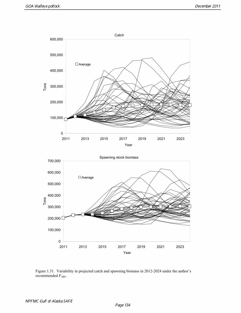
Catch

0

100,000

200,000

300,000

400,000

500,000

600,000

2011 2013 2015 2017 2019 2021 2023

Year

Tons

Average

Spawning stock biomass

0

100,000

200,000

300,000

400,000

500,000

600,000

700,000

2011 2013 2015 2017 2019 2021 2023Year

Tons

Average

Figure 1.31. Variability in projected catch and spawning biomass in 2012-2024 under the author’s recommended FABC.

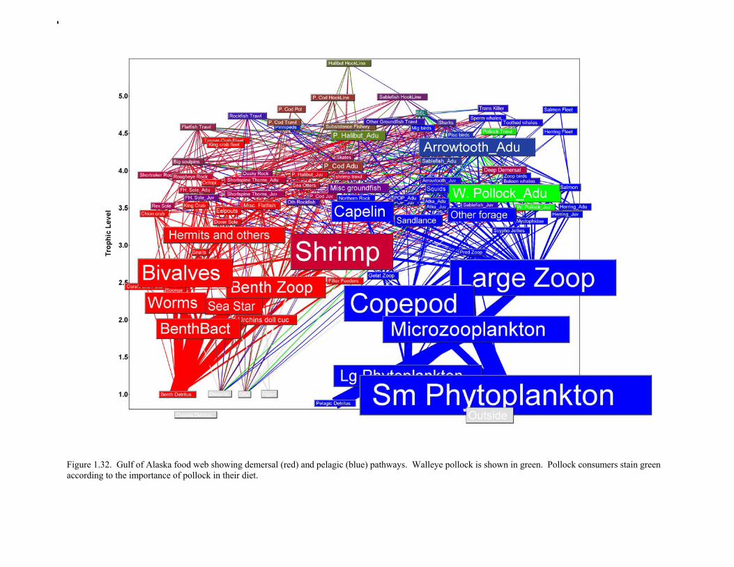
Figure 1.32. Gulf of Alaska food web showing demersal (red) and pelagic (blue) pathways. Walleye pollock is shown in green. Pollock consumers stain green according to the importance of pollock in their diet.

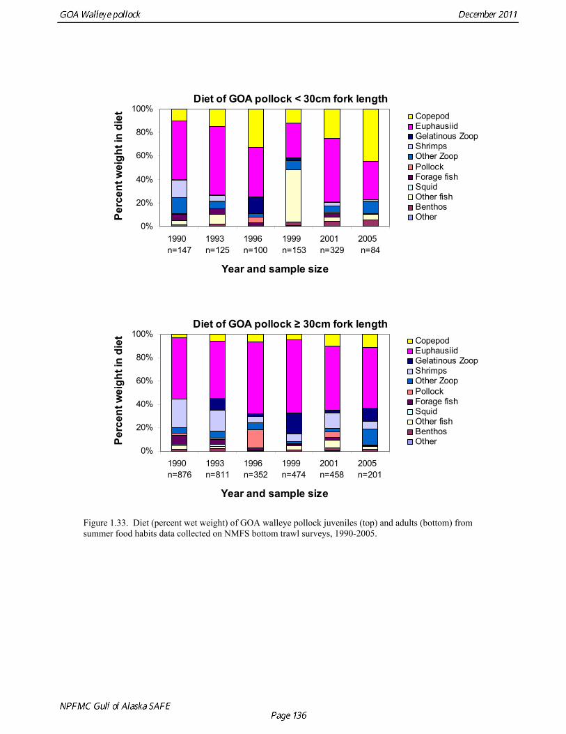
Diet of GOA pollock < 30cm fork length

0%

20%

40%

60%

80%

100%

1990 n=147

1993 n=125

1996 n=100

1999 n=153

2001 n=329

2005 n=84

Year and sample size

Perc

ent w

eigh

t in

diet Copepod

EuphausiidGelatinous ZoopShrimpsOther ZoopPollockForage fishSquidOther fishBenthosOther

Diet of GOA pollock ≥ 30cm fork length

0%

20%

40%

60%

80%

100%

1990 n=876

1993 n=811

1996 n=352

1999 n=474

2001 n=458

2005 n=201

Year and sample size

Perc

ent w

eigh

t in

diet Copepod

EuphausiidGelatinous ZoopShrimpsOther ZoopPollockForage fishSquidOther fishBenthosOther

Figure 1.33. Diet (percent wet weight) of GOA walleye pollock juveniles (top) and adults (bottom) from summer food habits data collected on NMFS bottom trawl surveys, 1990-2005.

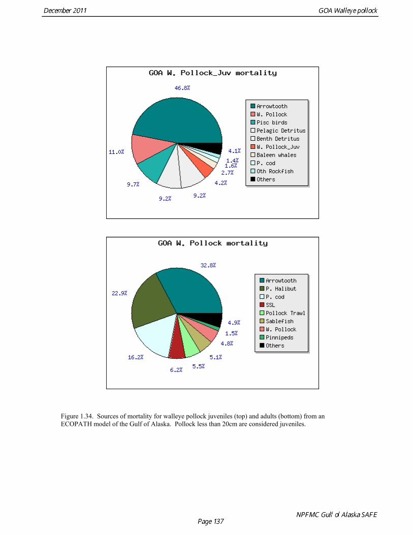
Figure 1.34. Sources of mortality for walleye pollock juveniles (top) and adults (bottom) from an ECOPATH model of the Gulf of Alaska. Pollock less than 20cm are considered juveniles.

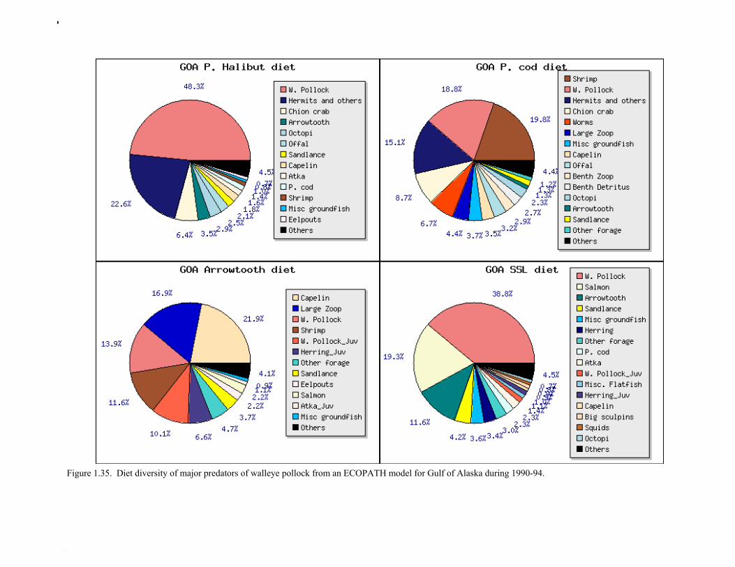
Figure 1.35. Diet diversity of major predators of walleye pollock from an ECOPATH model for Gulf of Alaska during 1990-94.

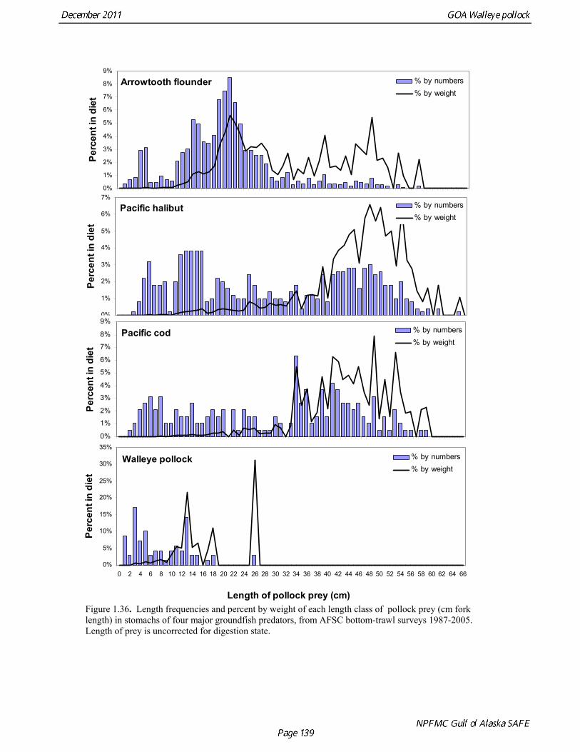
Arrowtooth flounder

0%

1%

2%

3%

4%

5%

6%

7%

8%

9%

0 2 4 6 8 10 12 14 16 18 20 22 24 26 28 30 32 34 36 38 40 42 44 46 48 50 52 54 56 58 60 62 64 66

% by numbers

Perc

ent i

n di

et% by weight

Pacific halibut

0%

1%

2%

3%

4%

5%

6%

7%

0 2 4 6 8 10 12 14 16 18 20 22 24 26 28 30 32 34 36 38 40 42 44 46 48 50 52 54 56 58 60 62 64 66

Perc

ent i

n di

et

% by numbers% by weight

Pacific cod

0%

1%

2%

3%

4%

5%

6%

7%

8%

9%

0 2 4 6 8 10 12 14 16 18 20 22 24 26 28 30 32 34 36 38 40 42 44 46 48 50 52 54 56 58 60 62 64 66

Perc

ent i

n di

et

% by numbers% by weight

Walleye pollock

0%

5%

10%

15%

20%

25%

30%

35%

0 2 4 6 8 10 12 14 16 18 20 22 24 26 28 30 32 34 36 38 40 42 44 46 48 50 52 54 56 58 60 62 64 66

Length of pollock prey (cm)

Perc

ent i

n di

et

% by numbers% by weight

Figure 1.36. Length frequencies and percent by weight of each length class of pollock prey (cm fork length) in stomachs of four major groundfish predators, from AFSC bottom-trawl surveys 1987-2005. Length of prey is uncorrected for digestion state.

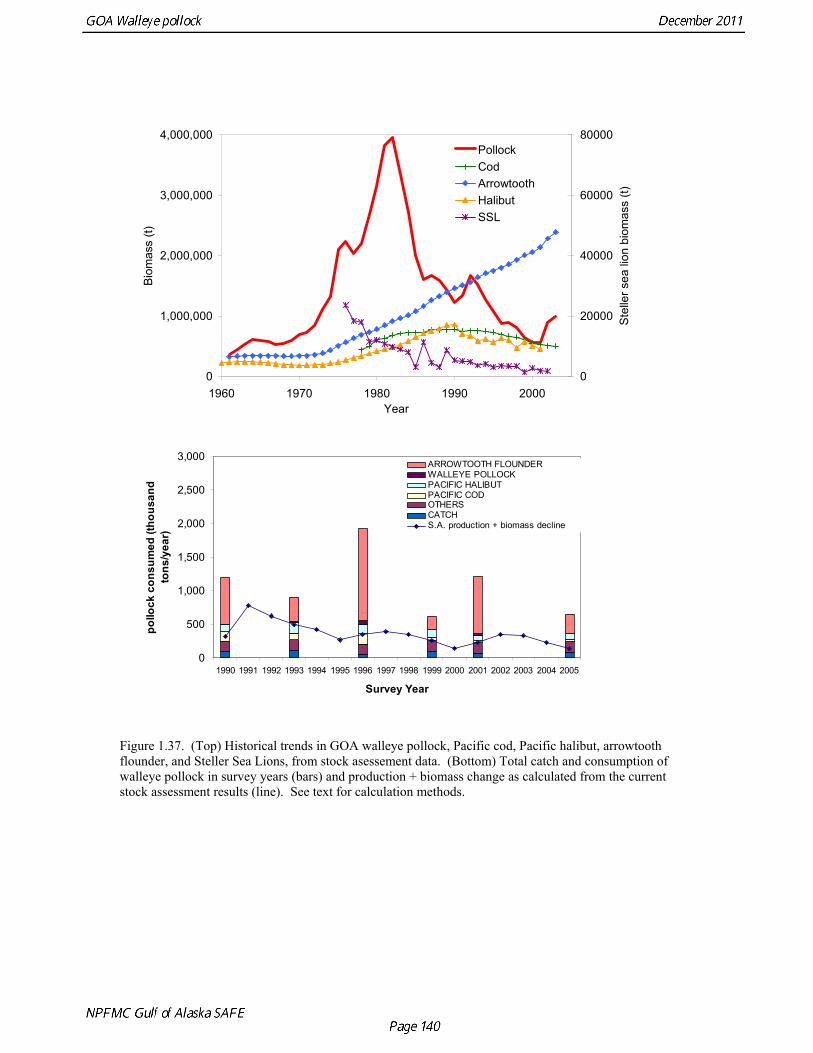
0

1,000,000

2,000,000

3,000,000

4,000,000

1960 1970 1980 1990 2000Year

Bio

mas

s (t)

0

20000

40000

60000

80000

Ste

ller s

ea li

on b

iom

ass

(t)

PollockCodArrowtoothHalibutSSL

0

500

1,000

1,500

2,000

2,500

3,000

1990 1991 1992 1993 1994 1995 1996 1997 1998 1999 2000 2001 2002 2003 2004 2005

Survey Year

pollo

ck c

onsu

med

(tho

usan

d to

ns/y

ear)

ARROWTOOTH FLOUNDERWALLEYE POLLOCKPACIFIC HALIBUTPACIFIC CODOTHERSCATCHS.A. production + biomass decline

Figure 1.37. (Top) Historical trends in GOA walleye pollock, Pacific cod, Pacific halibut, arrowtooth flounder, and Steller Sea Lions, from stock asessement data. (Bottom) Total catch and consumption of walleye pollock in survey years (bars) and production + biomass change as calculated from the current stock assessment results (line). See text for calculation methods.

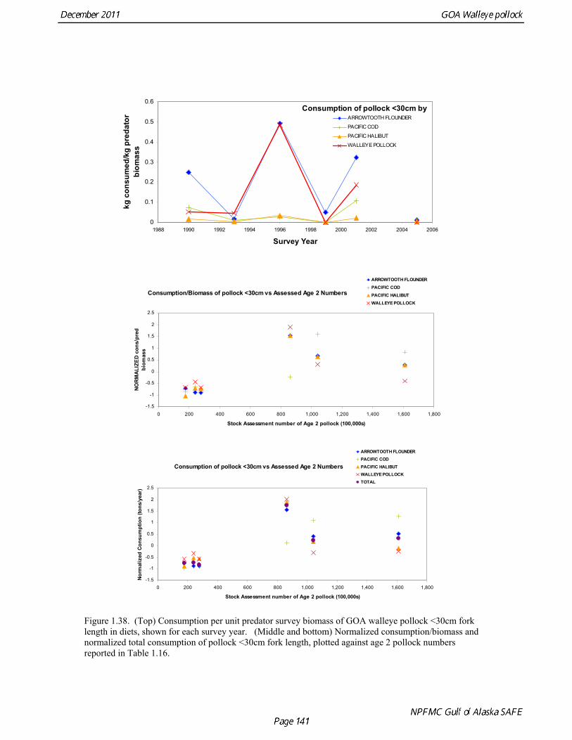
Consumption of pollock <30cm by

0

0.1

0.2

0.3

0.4

0.5

0.6

1988 1990 1992 1994 1996 1998 2000 2002 2004 2006

Survey Year

kg c

onsu

med

/kg

pred

ator

bi

omas

s

ARROWTOOTH FLOUNDER

PACIFIC COD

PACIFIC HALIBUT

WALLEYE POLLOCK

Consumption/Biomass of pollock <30cm vs Assessed Age 2 Numbers

-1.5

-1

-0.5

0

0.5

1

1.5

2

2.5

0 200 400 600 800 1,000 1,200 1,400 1,600 1,800

Stock Assessment number of Age 2 pollock (100,000s)

NORM

ALIZ

ED c

ons/

pred

biom

ass

ARROWTOOTH FLOUNDERPACIFIC COD

PACIFIC HALIBUTWALLEYE POLLOCK

Consumption of pollock <30cm vs Assessed Age 2 Numbers

-1.5

-1

-0.5

0

0.5

1

1.5

2

2.5

0 200 400 600 800 1,000 1,200 1,400 1,600 1,800

Stock Assessment number of Age 2 pollock (100,000s)

Norm

aliz

ed C

onsu

mpt

ion

(tons

/yea

r)

ARROWTOOTH FLOUNDERPACIFIC CODPACIFIC HALIBUTWALLEYE POLLOCKTOTAL

Figure 1.38. (Top) Consumption per unit predator survey biomass of GOA walleye pollock <30cm fork length in diets, shown for each survey year. (Middle and bottom) Normalized consumption/biomass and normalized total consumption of pollock <30cm fork length, plotted against age 2 pollock numbers reported in Table 1.16.

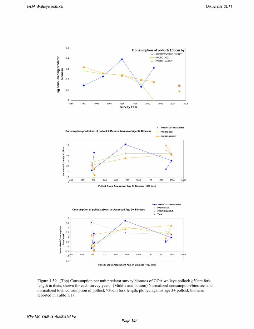
Consumption of pollock ≥30cm by

0

0.1

0.2

0.3

0.4

0.5

1988 1990 1992 1994 1996 1998 2000 2002 2004 2006Survey Year

kg c

onsu

med

/kg

pred

ator

bi

omas

s

ARROWTOOTH FLOUNDERPACIFIC CODPACIFIC HALIBUT

Consumption/pred biom. of pollock ≥30cm vs Assessed Age 3+ Biomass

-2

-1.5

-1

-0.5

0

0.5

1

1.5

2

400 500 600 700 800 900 1000 1100 1200 1300 1400

Pollock Stock Assessment Age 3+ Biomass (1000 tons)

Nor

mal

ized

con

s/pr

ed b

iom

ARROWTOOTH FLOUNDER

PACIFIC COD

PACIFIC HALIBUT

Consumption of pollock ≥30cm vs Assessed Age 3+ Biomass

-2.5

-2

-1.5

-1

-0.5

0

0.5

1

1.5

2

400 500 600 700 800 900 1000 1100 1200 1300 1400

Pollock Stock Assessment Age 3+ Biomass (1000 tons)

Nor

mal

ized

Con

sum

ptio

n (to

ns/y

ear)

ARROWTOOTH FLOUNDERPACIFIC CODPACIFIC HALIBUTTotal

Figure 1.39. (Top) Consumption per unit predator survey biomass of GOA walleye pollock ≥30cm fork length in diets, shown for each survey year. (Middle and bottom) Normalized consumption/biomass and normalized total consumption of pollock ≥30cm fork length, plotted against age 3+ pollock biomass reported in Table 1.17.

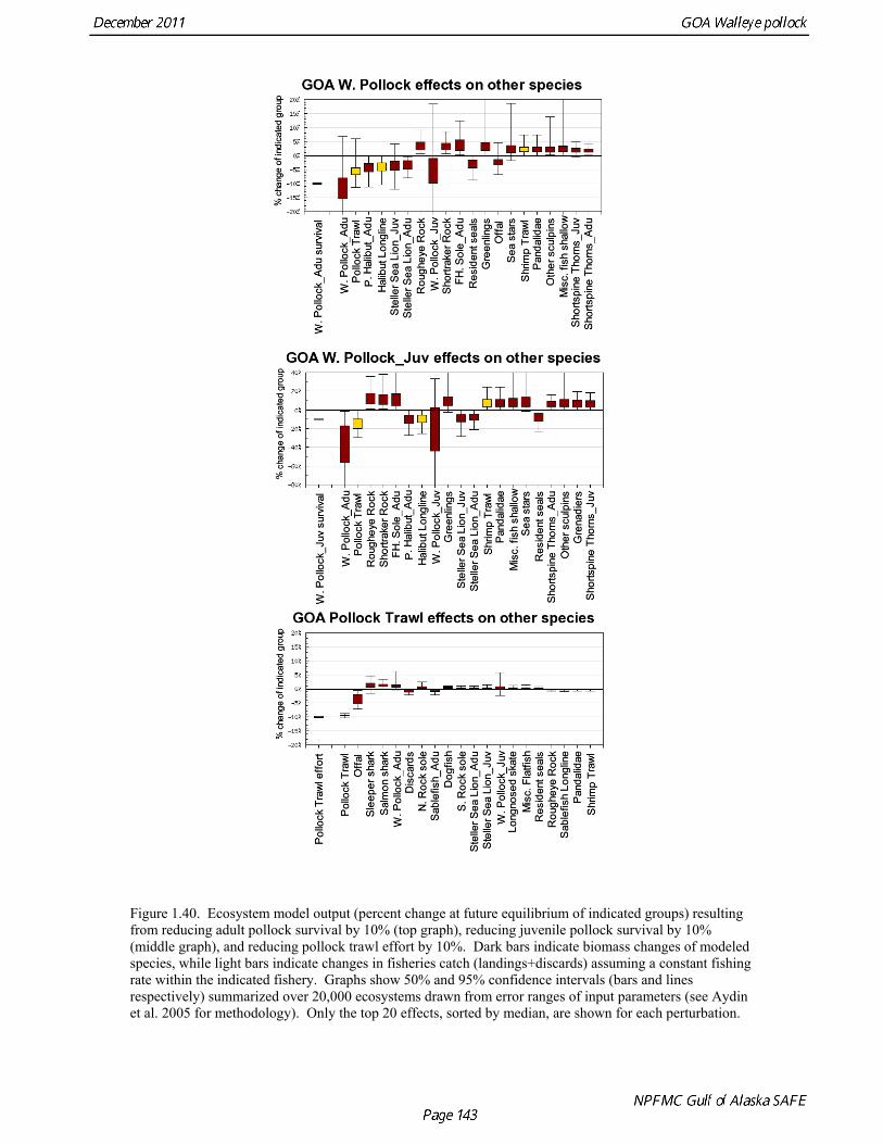
Figure 1.40. Ecosystem model output (percent change at future equilibrium of indicated groups) resulting from reducing adult pollock survival by 10% (top graph), reducing juvenile pollock survival by 10% (middle graph), and reducing pollock trawl effort by 10%. Dark bars indicate biomass changes of modeled species, while light bars indicate changes in fisheries catch (landings+discards) assuming a constant fishing rate within the indicated fishery. Graphs show 50% and 95% confidence intervals (bars and lines respectively) summarized over 20,000 ecosystems drawn from error ranges of input parameters (see Aydin et al. 2005 for methodology). Only the top 20 effects, sorted by median, are shown for each perturbation.

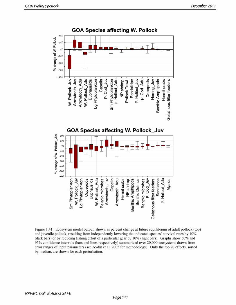
Figure 1.41. Ecosystem model output, shown as percent change at future equilibrium of adult pollock (top) and juvenile pollock, resulting from independently lowering the indicated species’ survival rates by 10% (dark bars) or by reducing fishing effort of a particular gear by 10% (light bars). Graphs show 50% and 95% confidence intervals (bars and lines respectively) summarized over 20,000 ecosystems drawn from error ranges of input parameters (see Aydin et al. 2005 for methodology). Only the top 20 effects, sorted by median, are shown for each perturbation.

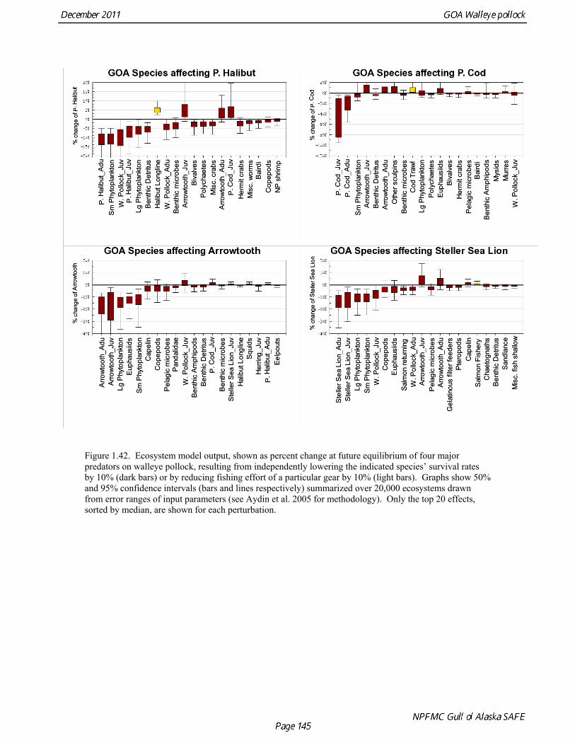
Figure 1.42. Ecosystem model output, shown as percent change at future equilibrium of four major predators on walleye pollock, resulting from independently lowering the indicated species’ survival rates by 10% (dark bars) or by reducing fishing effort of a particular gear by 10% (light bars). Graphs show 50% and 95% confidence intervals (bars and lines respectively) summarized over 20,000 ecosystems drawn from error ranges of input parameters (see Aydin et al. 2005 for methodology). Only the top 20 effects, sorted by median, are shown for each perturbation.

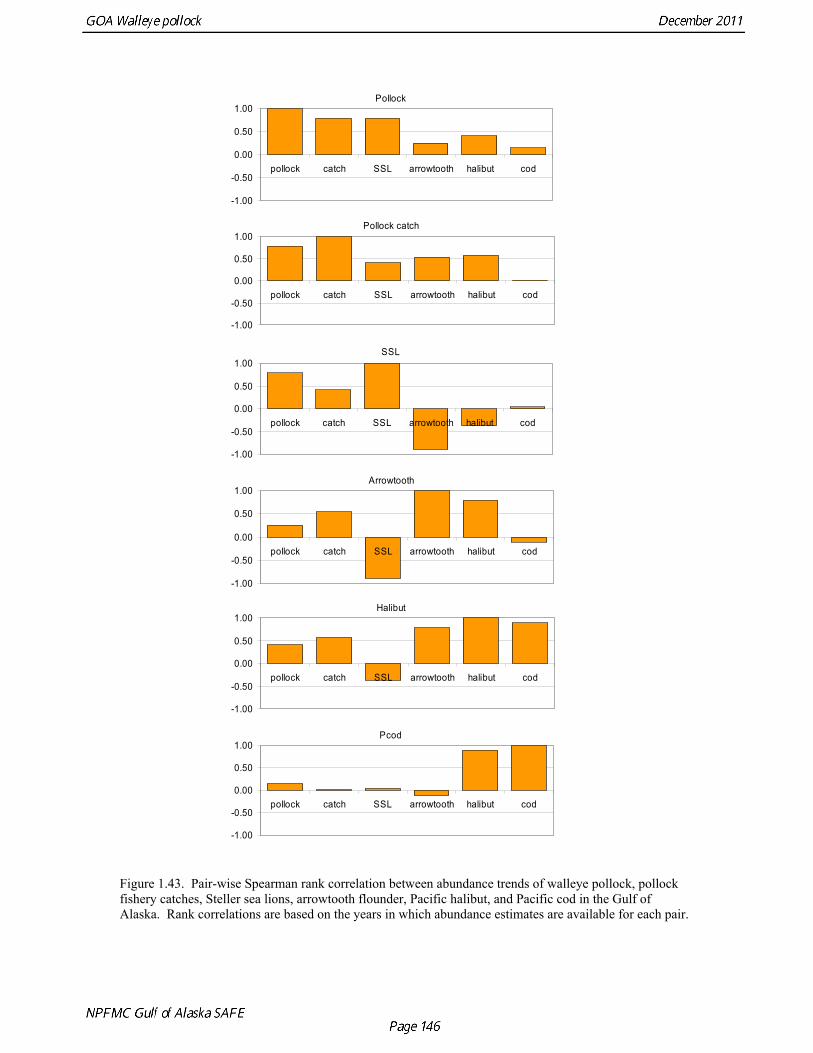
Arrowtooth

-1.00

-0.50

0.00

0.50

1.00

pollock catch SSL arrowtooth halibut cod

Halibut

-1.00

-0.50

0.00

0.50

1.00

pollock catch SSL arrowtooth halibut cod

Pollock

-1.00

-0.50

0.00

0.50

1.00

pollock catch SSL arrowtooth halibut cod

Pollock catch

-1.00

-0.50

0.00

0.50

1.00

pollock catch SSL arrowtooth halibut cod

SSL

-1.00

-0.50

0.00

0.50

1.00

pollock catch SSL arrowtooth halibut cod

Pcod

-1.00

-0.50

0.00

0.50

1.00

pollock catch SSL arrowtooth halibut cod

Figure 1.43. Pair-wise Spearman rank correlation between abundance trends of walleye pollock, pollock fishery catches, Steller sea lions, arrowtooth flounder, Pacific halibut, and Pacific cod in the Gulf of Alaska. Rank correlations are based on the years in which abundance estimates are available for each pair.

Appendix A: Southeast Alaska pollock Bottom trawl surveys indicate a substantial reduction in pollock abundance east of 140° W. lon. Stock structure in this area is poorly understood. Bailey et al. (1999) suggest that pollock metapopulation structure in southeast Alaska is characterized by numerous fiord populations. In the 2009 bottom trawl survey, higher pollock CPUE in southeast Alaska occurred primarily from Cape Ommaney to Dixon Entrance, where the shelf is more extensive. Pollock length composition in the 2011 bottom trawl survey is dominated by age-1 pollock, with progressively decreasing proportions of larger pollock (Appendix Fig. 1.1). There are very few larger pollock (> 50 cm). Juveniles in this area are unlikely to influence the population dynamics of pollock in the central and western Gulf of Alaska. Ocean currents are generally northward in this area, suggesting that juvenile settlement is a result of spawning further south. Spawning aggregations of pollock have been reported from the northern part of Dixon Entrance (Saunders et al. 1988). Historically, there has been little directed fishing for pollock in Southeast Alaska (Fritz 1993). Pollock catch the Southeast and East Yakutat statistical areas has averaged about 1 t since 2000 (Table 1.4). The ban on trawling east of 140° W. lon. prevents the development of a trawl fishery for pollock in Southeast Alaska. Pollock biomass estimates from the bottom trawl survey are variable, in part due to year-to-year differences in survey coverage. Biomass in Southeast Alaska was estimated by splitting survey strata and CPUE data in the Yakutat INPFC area at 140° W. lon. and combining the strata east of the line with comparable strata in the Southeastern INPFC area. Surveys since 1996 had the most complete coverage of shallow strata in southeast Alaska, and indicate that stock size is approximately 25-75,000 t (Appendix Figure 1.1). There are gradual increasing trend in biomass since 2005, but confidence intervals for biomass are large. We recommend placing southeast Alaska pollock in Tier 5 of NPFMC harvest policy, and basing the ABC and OFL on natural mortality (0.3) and the biomass for the 2011 survey (47,885 t). This results in a 2012 ABC of 10,774 t (47,885 t * 0.75 M), and a 2012 OFL of 14,366 t (47,885 t * M).

0

20,000

40,000

60,000

80,000

100,000

120,000

1988 1992 1996 2000 2004 2008 2012Year

Bio

mas

s (t)

0

0.03

0.06

0.09

5 10 15 20 25 30 35 40 45 50 55 60 65 70 75Length (cm)

Appendix Figure 1.1. Pollock size composition in 2011 (left) and biomass trend in southeast Alaska from NMFS bottom trawl surveys in 1990-2011 (right). Error bars indicate plus and minus two standard deviations.

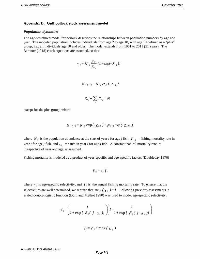
Appendix B: Gulf pollock stock assessment model

Population dynamics The age-structured model for pollock describes the relationships between population numbers by age and year. The modeled population includes individuals from age 2 to age 10, with age 10 defined as a Aplus@ group, i.e., all individuals age 10 and older. The model extends from 1961 to 2011 (51 years). The Baranov (1918) catch equations are assumed, so that

)]Z(- - [1 ZF N = c j i

j i

j ij ij i exp

) Z(- N = N j ij i1+j 1+i exp

M+ F = Z j i

kj i ∑

except for the plus group, where

) Z(- N + ) Z(- N = N 10 i,10 i,9 i,9 i,10 1,+i expexp where is the population abundance at the start of year i for age j fish, = fishing mortality rate in year i for age j fish, and = catch in year i for age j fish. A constant natural mortality rate, M, irrespective of year and age, is assumed.

N j i F j i

c j i

Fishing mortality is modeled as a product of year-specific and age-specific factors (Doubleday 1976)

f s = F ijij

where is age-specific selectivity, and is the annual fishing mortality rate. To ensure that the selectivities are well determined, we require that . Following previous assessments, a scaled double-logistic function (Dorn and Methot 1990) was used to model age-specific selectivity,

s j f i

1 = ) s ( j max

⎟⎟⎠

⎞⎜⎜⎝

⎛⎟⎟⎠

⎞⎜⎜⎝

⎛′

)] -j ( [- + 11 - 1

)] -j ( [- + 11 = s

2211j

αβαβ expexp

) s ( / s = s jjj ′′ max

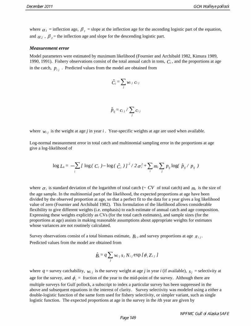
where α1 = inflection age, β 1 = slope at the inflection age for the ascending logistic part of the eand

quation,

α 2 , β 2 = the inflection age and slope for the descending logistic part.

Measurement error Model parameters were estimated by maximum likelihood (Fournier and Archibald 1982, Kimura 1989, 1990, 1991). Fishery observations consist of the total annual catch in tons, , and the proportions at age in the catch, . Predicted values from the model are obtained from

Ci

p j i

cw = C j ij ij

i ∑ˆ

c / c = p j ij

j iij ∑ˆ

where is the weight at age j in year i . Year-specific weights at age are used when available. w j i

Log-normal measurement error in total catch and multinomial sampling error in the proportions at age give a log-likelihood of

) p / p ( p m + 2 / ]) C ( ) C ( [ = L ijijijj

ii

2i

2 ii

ik ˆlogˆlogloglog ∑∑∑− − σ

where σ i is standard deviation of the logarithm of total catch (~ CV of total catch) and is the size of the age sample. In the multinomial part of the likelihood, the expected proportions at age have been divided by the observed proportion at age, so that a perfect fit to the data for a year gives a log likelihood value of zero (Fournier and Archibald 1982). This formulation of the likelihood allows considerable flexibility to give different weights (i.e. emphasis) to each estimate of annual catch and age composition. Expressing these weights explicitly as CVs (for the total catch estimates), and sample sizes (for the proportions at age) assists in making reasonable assumptions about appropriate weights for estimates whose variances are not routinely calculated.

mi

Survey observations consist of a total biomass estimate, , and survey proportions at age Bi π j i . Predicted values from the model are obtained from

] Z [ N s w q = B j iij ijj ij

i φexpˆ ∑

where = survey catchability, is the survey weight at age j in year i (if available), s = selectivity at age for the survey, and

q w j i j

φ i = fraction of the year to the mid-point of the survey. Although there are multiple surveys for Gulf pollock, a subscript to index a particular survey has been suppressed in the above and subsequent equations in the interest of clarity. Survey selectivity was modeled using a either a double-logistic function of the same form used for fishery selectivity, or simpler variant, such as single logistic function. The expected proportions at age in the survey in the ith year are given by

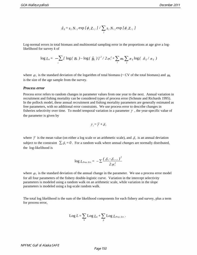
Log-normal errors in total biomass and multinomial sampling error in the proportions at age give a log-likelihood for survey k of

where

] Z [ N s /] Z [ N s = j iij ijj

j iij ijij φφπ expexpˆ ∑

) / ( m + 2 / ]) B ( ) B ( [ = L ijijijj

ii

2i

2 ii

ik πππσ ˆlogˆlogloglog ∑∑∑− −

σ i is the standard deviation of the logarithm of total biomass (~ CV of the total biomass) and

age sample from the survey.

995). te

ditional error constraints. We use process error to describe changes in fisheries selectivity over time. To model temporal variation in a parameter

mi is the size of the

Process error Process error refers to random changes in parameter values from one year to the next. Annual variation in recruitment and fishing mortality can be considered types of process error (Schnute and Richards 1In the pollock model, these annual recruitment and fishing mortality parame rs are generally estimated asfree parameters, with no ad

γ , the year-specific value of the parameter is given by

δγγ ii + =

where γ is the mean value (on either a log scale or an arithmetic scale), and δ i is an annual deviation subject to the constraint 0 = iδ∑ . For a random walk where annual changes are normally distributed, the log-likelihood is

σ 2i

Err. Proc. 2δδ 1 + ii

2 ) - ( = L ∑−log

where σ i is the standard deviation of the annual change in the parameter. We use a process errofor all four parameters of the fishery double-logistic cur

r model ve. Variation in the intercept selectivity

arameters is modeled using a random walk on an arithmetic scale, while variation in the slope arameters is modeled using a log-scale random walk.

he total log likelihood is the sum of the likelihood components for each fishery and survey, plus a term for process error,

pp T

. L + L = L Err. Proc.p

kk

LogLogLog ∑∑

Appendix C: Seasonal distribution and apportionment of walleye pollock among management areas in the Gulf of Alaska Since 1992, the Gulf of Alaska pollock TAC has been apportioned between management areas based on the distribution of biomass in groundfish surveys. Both single species and ecosystem considerations provide the rationale for apportioning the TAC. From an ecosystem perspective, apportioning the TAC will spatially distribute the effects of fishing on other pollock consumers (i.e., Steller sea lions), potentially reducing the overall intensity of any averse effects. Apportioning the TAC also ensures that no smaller component of the stock experiences higher mortality than any other. Although no sub-stock units of pollock have yet been identified in the Gulf of Alaska, it would be precautionary to manage the fishery so that if these sub-units do exist they would not be subject to high fishing mortality. Protection of sub-stock units would be most important during spawning season, when they are spatially separated. The Steller sea lion protection measures implemented in 2001 require apportionment of pollock TAC based on the seasonal distribution of biomass. Although spatial apportionment is intended to reduce the potential impact of fishing on endangered Steller sea lions, it is important to recognize that apportioning the TAC based on an inaccurate or inappropriate estimate of biomass distribution could be detrimental, both to pollock population itself, and on species that depend on pollock. Walleye pollock in the Gulf of Alaska undergo an annual migration between summer foraging habitats and winter spawning grounds. Since surveying effort has been concentrated during the summer months and prior to spawning in late winter, the dynamics and timing of this migration are not well understood. Regional biomass estimates are highly variable, indicating either large sampling variability, large interannual changes in distribution, or, more likely, both. There is a comprehensive survey of the Gulf of Alaska in summer, but historically surveying during winter has focused on the Shelikof Strait spawning grounds. Recently there has been expanded EIT surveying effort outside of Shelikof Strait in winter, but no acoustic survey has been comprehensive, covering all areas where pollock could potentially occur.

Winter distribution An annual acoustic survey on pre-spawning aggregations in Shelikof Strait has been conducted since 1981. Since 2000, several additional spawning areas have been surveyed multiple times, including Sanak Gully, the Shumagin Islands, the shelf break near Chirikof Island, and Marmot Bay. Although none of these spawning grounds are as important as Shelikof Strait, especially from a historical perspective, in recent years the aggregate biomass surveyed outside Shelikof Strait has been comparable to that within Shelikof Strait. As in previous assessments, a “composite” approach was used to estimate the percent of the total stock in each management area. The estimated biomass for each survey was divided by the total biomass of pollock estimated by the assessment model in that year and then split into management areas for surveys that crossed management boundaries. The percent for each survey was added together to form a composite biomass distribution, which was then rescaled so that it summed to 100%. Model estimates of biomass at spawning took into account the total mortality between the start of the year and spawning, and used mean weight at age from Shelikof Strait surveys. Since no winter surveys were conducted in 2011, estimates of the percentage by area could not be updated with recent survey information. Since time series of biomass estimates for spawning areas outside of Shelikof Strait are now available, we used the four most recent surveys at each spawning area, and used a rule that a minimum of three surveys was necessary to include an area. These criteria are intended to provide estimates that reflect recent biomass distribution while at the same time providing some stability in the estimates. The biomass in these secondary spawning areas tends to be highly variable from one year to the next. Areas meeting these criteria were Shelikof Strait, the shelf break near Chirikof Island, the Shumagin area, Sanak Gully, Morzhovoi Bay, and Marmot Bay. We excluded an acoustic survey in 1990 along the shelf break and on east side of Kodiak Island (Karp 1990), since this information is more than 20 years old and the survey overlaps with some of the other areas included in the calculations. While the spawning aggregations

found in 2010 along the Kenai Peninsula and in Prince William Sound are clearly important, before including them in the apportionment calculations the surveys in these areas need to be repeated to confirm stability of spawning in these areas There are also several potentially difficult issues that would need to dealt with, for example, whether including biomass along Kenai Peninsula would lead increased harvests on the east side of Kodiak, both of which are in area 630. In addition, the fishery inside Prince William Sound (area 649) is managed by the State of Alaska, and state management objectives for Prince William Sound need to be taken into account. Vessel comparison experiments conducted between the R/V Miller Freeman and the R/V Oscar Dyson in Shelikof Strait in 2007, and in the Shumagin/Sanak area in 2008 found significant differences in the ratio of backscatter between the two vessels. The estimated R/V Oscar Dyson to R/V Miller Freeman ratio for the Shelikof Strait was 1.132, while the ratio for the Shumagin and Sanak areas (taken together) was 1.31. Since the R/V Oscar Dyson was designed to minimize vessel avoidance, biomass estimates produced by R/V Oscar Dyson should be considered better estimates of the true biomass than those produced by the R/V Miller Freeman. These results imply that the biomass in the western GOA (Sanak and Shumagin areas) has historically been underestimated relative to the central GOA. The leading hypothesis for the higher ratio in the western GOA is that the fish are distributed shallower than in Shelikof Strait, and consequently are exposed to a stronger stimulus from the vessel. When calculating the distribution of biomass by area, multipliers were applied to surveys conducted by the R/V Miller Freeman to make them comparable to the R/V Oscar Dyson (Appendix table 1.1). No vessel comparisons were conducted in the Chirikof area, Marmot Bay, or Morzhovoi Bay. A vessel specific multiplier of 1.0 was applied in the Chirikof area as differential avoidance is not expected at fish depths observed in the Chirikof area, where pollock are distributed primarily at depths greater than 300 m (e.g. in 2008 90% of pollock biomass was deeper than 275 m). A vessel specific multiplier of 1.31 was applied in Marmot Bay and Morzhovoi Bay because the fish in these areas were at similar depths as at the Sanak and Shumagin area. The sum of the percent biomass for all surveys combined was 63.38%, which may reflect sampling variability, or interannual variation in spawning location, but also reflects the recent trend that the aggregate biomass of pollock surveyed acoustically in winter (at least in those area that have been surveyed repeatedly) is lower than the assessment model estimates of abundance. After rescaling, the resulting average biomass distribution was 22.64%, 67.25%, 10.11% in areas 610, 620, and 630 (Appendix table 1.1). In comparison to last year’s assessment, the percentages by area are nearly identical due to the lack of new survey data.

A-season apportionment between areas 620 and 630

In the 2002 assessment, based on evaluation of fishing patterns which suggested that the migration to spawning areas was not complete by January 20, the plan team recommended an alternative apportionment scheme for areas 620 and 630 based on the midpoint of the summer and winter distributions in area 630. This approach was not used for area 610 because fishing patterns during the A season suggested that most of the fish captured in area 610 would eventually spawn in area 610. The resulting A season apportionment using updated survey data is: 610, 22.64%; 620, 54.76%; 630, 22.60%.

Middleton Island winter EIT survey results in 2003

The apportionment for area 640, which is not managed by season, has previously been based on the summer distribution of the biomass. Fishing, however, takes places primarily in winter or early spring on a spawning aggregation near Middleton Island. During 28-29 March 2003, this area was surveyed by the NOAA ship Miller Freeman for the first time and biomass estimate of 6,900 t was obtained. Although maturity stage data suggested the timing of the survey was appropriate, discussions with fishing vessels contacted during the survey raised some questions about survey timing relative to peak biomass. Notwithstanding, a tier 5 calculation based on this spawning biomass gives an ABC of 1,550 t (6,901 t * 0.75 M), compared to 3,277 t for the author’s 2012 ABC recommendation and an apportionment based on

the summer biomass distribution. This suggests that the current approach of basing the area 640 apportionment on the gulfwide ABC and the summer biomass distribution is at least consistent with the biomass present near Middleton Island in the winter. We recommend continuing this approach until sufficient survey information during winter has accumulated to evaluate interannual variation in the biomass present in this area.

Summer distribution

The NMFS bottom trawl is summer survey (typically extending from mid-May to mid-August). Because of large shifts in the distribution of pollock between management areas one survey to the next, and the high variance of biomass estimates by management area, Dorn et al. (1999) recommended that the apportionment of pollock TAC be based upon an unweighted average of four most recent NMFS summer surveys. The four-survey average was updated with 2011 survey results in an average biomass distribution of 35.35%, 27.57%, 34.02%, and 3.07% in areas 610, 620, 630, and 640 (Appendix Fig. 1.2). Including the 2011 survey and deleting the 2003 survey lowered the percentage in area 610 by 5 percentage points and raised the percentage in areas 620 and 630 by 2 and 3 percentage points respectively.

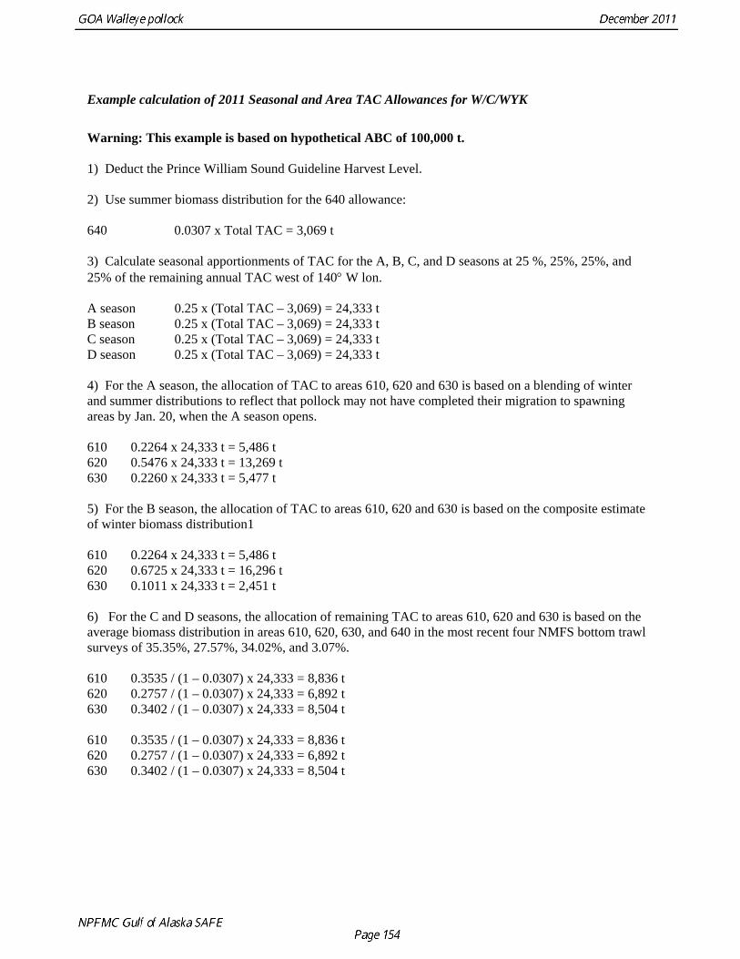
Example calculation of 2011 Seasonal and Area TAC Allowances for W/C/WYK

Warning: This example is based on hypothetical ABC of 100,000 t. 1) Deduct the Prince William Sound Guideline Harvest Level. 2) Use summer biomass distribution for the 640 allowance: 640 0.0307 x Total TAC = 3,069 t 3) Calculate seasonal apportionments of TAC for the A, B, C, and D seasons at 25 %, 25%, 25%, and 25% of the remaining annual TAC west of 140° W lon. A season 0.25 x (Total TAC – 3,069) = 24,333 t B season 0.25 x (Total TAC – 3,069) = 24,333 t C season 0.25 x (Total TAC – 3,069) = 24,333 t D season 0.25 x (Total TAC – 3,069) = 24,333 t 4) For the A season, the allocation of TAC to areas 610, 620 and 630 is based on a blending of winter and summer distributions to reflect that pollock may not have completed their migration to spawning areas by Jan. 20, when the A season opens. 610 0.2264 x 24,333 t = 5,486 t 620 0.5476 x 24,333 t = 13,269 t 630 0.2260 x 24,333 t = 5,477 t 5) For the B season, the allocation of TAC to areas 610, 620 and 630 is based on the composite estimate of winter biomass distribution1 610 0.2264 x 24,333 t = 5,486 t 620 0.6725 x 24,333 t = 16,296 t 630 0.1011 x 24,333 t = 2,451 t 6) For the C and D seasons, the allocation of remaining TAC to areas 610, 620 and 630 is based on the average biomass distribution in areas 610, 620, 630, and 640 in the most recent four NMFS bottom trawl surveys of 35.35%, 27.57%, 34.02%, and 3.07%. 610 0.3535 / (1 – 0.0307) x 24,333 = 8,836 t 620 0.2757 / (1 – 0.0307) x 24,333 = 6,892 t 630 0.3402 / (1 – 0.0307) x 24,333 = 8,504 t 610 0.3535 / (1 – 0.0307) x 24,333 = 8,836 t 620 0.2757 / (1 – 0.0307) x 24,333 = 6,892 t 630 0.3402 / (1 – 0.0307) x 24,333 = 8,504 t

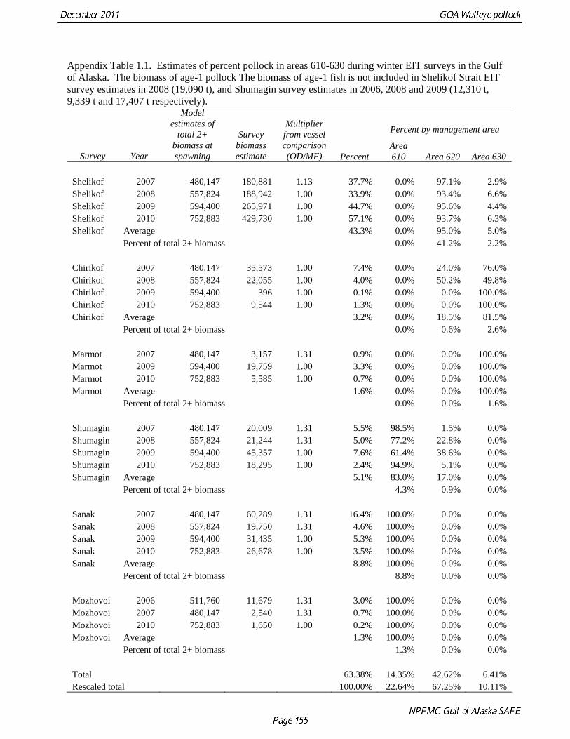
Appendix Table 1.1. Estimates of percent pollock in areas 610-630 during winter EIT surveys in the Gulf of Alaska. The biomass of age-1 pollock The biomass of age-1 fish is not included in Shelikof Strait EIT survey estimates in 2008 (19,090 t), and Shumagin survey estimates in 2006, 2008 and 2009 (12,310 t, 9,339 t and 17,407 t respectively).

Percent by management area

Survey Year

Model estimates of

total 2+ biomass at spawning

Survey biomass estimate

Multiplier from vessel comparison (OD/MF) Percent

Area 610 Area 620 Area 630

Shelikof 2007 480,147 180,881 1.13 37.7% 0.0% 97.1% 2.9% Shelikof 2008 557,824 188,942 1.00 33.9% 0.0% 93.4% 6.6% Shelikof 2009 594,400 265,971 1.00 44.7% 0.0% 95.6% 4.4% Shelikof 2010 752,883 429,730 1.00 57.1% 0.0% 93.7% 6.3% Shelikof Average 43.3% 0.0% 95.0% 5.0% Percent of total 2+ biomass 0.0% 41.2% 2.2% Chirikof 2007 480,147 35,573 1.00 7.4% 0.0% 24.0% 76.0% Chirikof 2008 557,824 22,055 1.00 4.0% 0.0% 50.2% 49.8% Chirikof 2009 594,400 396 1.00 0.1% 0.0% 0.0% 100.0% Chirikof 2010 752,883 9,544 1.00 1.3% 0.0% 0.0% 100.0% Chirikof Average 3.2% 0.0% 18.5% 81.5% Percent of total 2+ biomass 0.0% 0.6% 2.6% Marmot 2007 480,147 3,157 1.31 0.9% 0.0% 0.0% 100.0% Marmot 2009 594,400 19,759 1.00 3.3% 0.0% 0.0% 100.0% Marmot 2010 752,883 5,585 1.00 0.7% 0.0% 0.0% 100.0% Marmot Average 1.6% 0.0% 0.0% 100.0% Percent of total 2+ biomass 0.0% 0.0% 1.6% Shumagin 2007 480,147 20,009 1.31 5.5% 98.5% 1.5% 0.0% Shumagin 2008 557,824 21,244 1.31 5.0% 77.2% 22.8% 0.0% Shumagin 2009 594,400 45,357 1.00 7.6% 61.4% 38.6% 0.0% Shumagin 2010 752,883 18,295 1.00 2.4% 94.9% 5.1% 0.0% Shumagin Average 5.1% 83.0% 17.0% 0.0% Percent of total 2+ biomass 4.3% 0.9% 0.0% Sanak 2007 480,147 60,289 1.31 16.4% 100.0% 0.0% 0.0% Sanak 2008 557,824 19,750 1.31 4.6% 100.0% 0.0% 0.0% Sanak 2009 594,400 31,435 1.00 5.3% 100.0% 0.0% 0.0% Sanak 2010 752,883 26,678 1.00 3.5% 100.0% 0.0% 0.0% Sanak Average 8.8% 100.0% 0.0% 0.0% Percent of total 2+ biomass 8.8% 0.0% 0.0% Mozhovoi 2006 511,760 11,679 1.31 3.0% 100.0% 0.0% 0.0% Mozhovoi 2007 480,147 2,540 1.31 0.7% 100.0% 0.0% 0.0% Mozhovoi 2010 752,883 1,650 1.00 0.2% 100.0% 0.0% 0.0% Mozhovoi Average 1.3% 100.0% 0.0% 0.0% Percent of total 2+ biomass 1.3% 0.0% 0.0% Total 63.38% 14.35% 42.62% 6.41% Rescaled total 100.00% 22.64% 67.25% 10.11%

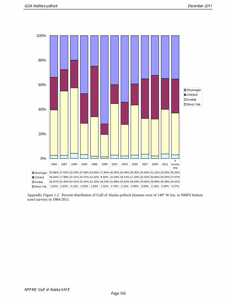
0%

20%

40%

60%

80%

100%

ShumaginChirikofKodiakWest Yak.

Shumagin 33.88% 27.60% 20.03% 47.08% 24.69% 71.90% 40.06% 54.09% 39.35% 34.94% 32.16% 34.93% 35.35%

Chirikof 26.64% 17.38% 22.41% 24.27% 41.32% 8.55% 15.30% 18.14% 17.16% 32.42% 35.66% 25.04% 27.57%

Kodiak 36.87% 52.40% 53.42% 25.44% 32.16% 18.23% 41.88% 25.62% 40.64% 29.06% 29.99% 36.38% 34.02%

West Yak. 2.62% 2.62% 4.13% 3.20% 1.83% 1.32% 2.76% 2.15% 2.85% 3.59% 2.18% 3.65% 3.07%

1984 1987 1990 1993 1996 1999 2001 2003 2005 2007 2009 20114

survey avg

Appendix Figure 1.2. Percent distribution of Gulf of Alaska pollock biomass west of 140° W lon. in NMFS bottom trawl surveys in 1984-2011.

Appendix D: Supplemental catch data To comply with the Annual Catch Limit (ACL) requirements, two new datasets have been generated to help estimate total catch and removals from NMFS stocks in Alaska. The first data set is more a comprehensive accounting of research removals than had been available previously. This data set is available only for 2010. The second data set provides estimates of incidental catch of groundfish in the Pacific halibut fishery during 2001-2010 using methods described in Tribuzio et. al (2011). Since some halibut fishery incidental catch as enters into the catch accounting system, it is unclear whether these catches have already been taken into account in the reported catch. However this seems unlikely for pollock. Research catches have been routinely reported in the pollock assessment, but these catches are only for survey data that have been included in RACEBASE, and are not a comprehensive accounting of all research removals. Supplemental pollock catch data are presented in several tables. Appendix Table 1.2 provides research catches from RACEBASE for the period 1977-2011. Appendix Table 1.3 provides research catch by survey or research project for 2010. Appendix Table 1.4 provides incidental catches for the halibut fishery. Comparison of research catches from RACEBASE with the more comprehensive information in 2010 suggests that research catches have been substantially underreported. The estimates from RACEBACE in 2010 are approximately 25% of the total research catch. Annual large-mesh and small-mesh trawl surveys conducted by ADG&G account for most of the missing research catch of pollock. Even if research catches are four times those reported in RACEBACE, they would still amount to less than 1/2 of a percent on average of the ABC during 2002-2011, and would have a negligible effect on the pollock stock and the stock assessment. Unreported catches in the halibut fishery are lower, and would likewise have a negligible effect. It is important to note that there is unreported incidental catch of pollock in other fisheries in Alaska, such as the salmon fishery, which, based on anecdotal reports, may be substantial on occasion.

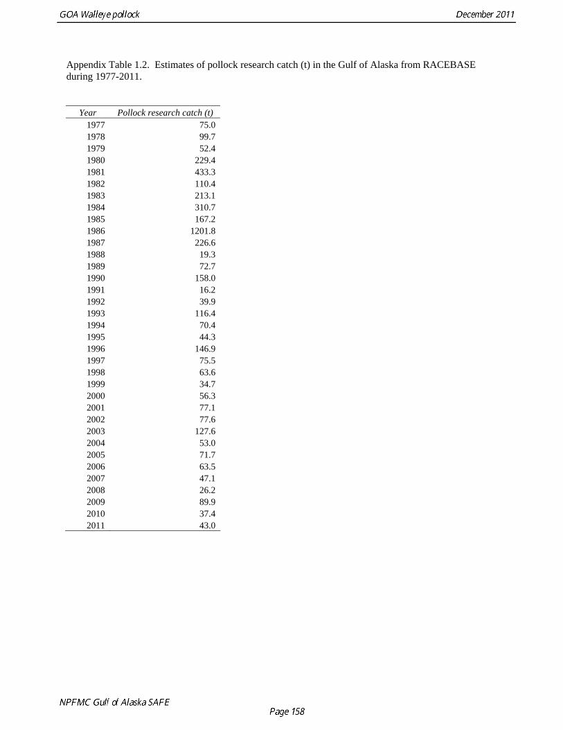
Appendix Table 1.2. Estimates of pollock research catch (t) in the Gulf of Alaska from RACEBASE during 1977-2011.

Year Pollock research catch (t) 1977 75.0 1978 99.7 1979 52.4 1980 229.4 1981 433.3 1982 110.4 1983 213.1 1984 310.7 1985 167.2 1986 1201.8 1987 226.6 1988 19.3 1989 72.7 1990 158.0 1991 16.2 1992 39.9 1993 116.4 1994 70.4 1995 44.3 1996 146.9 1997 75.5 1998 63.6 1999 34.7 2000 56.3 2001 77.1 2002 77.6 2003 127.6 2004 53.0 2005 71.7 2006 63.5 2007 47.1 2008 26.2 2009 89.9 2010 37.4 2011 43.0

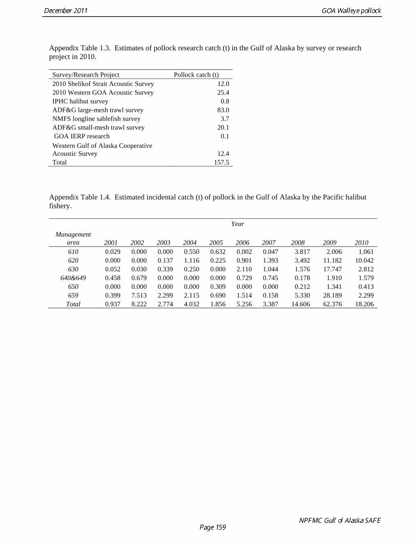
Appendix Table 1.3. Estimates of pollock research catch (t) in the Gulf of Alaska by survey or research project in 2010. Survey/Research Project Pollock catch (t) 2010 Shelikof Strait Acoustic Survey 12.0 2010 Western GOA Acoustic Survey 25.4 IPHC halibut survey 0.8 ADF&G large-mesh trawl survey 83.0 NMFS longline sablefish survey 3.7 ADF&G small-mesh trawl survey 20.1 GOA IERP research 0.1 Western Gulf of Alaska Cooperative Acoustic Survey 12.4 Total 157.5

Appendix Table 1.4. Estimated incidental catch (t) of pollock in the Gulf of Alaska by the Pacific halibut fishery.

Year Management

area 2001 2002 2003 2004 2005 2006 2007 2008 2009 2010 610 0.029 0.000 0.000 0.550 0.632 0.002 0.047 3.817 2.006 1.061 620 0.000 0.000 0.137 1.116 0.225 0.901 1.393 3.492 11.182 10.042 630 0.052 0.030 0.339 0.250 0.000 2.110 1.044 1.576 17.747 2.812

640&649 0.458 0.679 0.000 0.000 0.000 0.729 0.745 0.178 1.910 1.579 650 0.000 0.000 0.000 0.000 0.309 0.000 0.000 0.212 1.341 0.413 659 0.399 7.513 2.299 2.115 0.690 1.514 0.158 5.330 28.189 2.299

Total 0.937 8.222 2.774 4.032 1.856 5.256 3.387 14.606 62.376 18.206

(This page intentionally left blank)