Chapter 1: Assessment of the Walleye Pollock Stock in the Gulf of Alaska

Martin Dorn1, Kerim Aydin1, Benjamin Fissel1, Darin Jones1, Abigail McCarthy1,

Wayne Palsson1, and Kally Spalinger2

1 National Marine Fisheries Service, Alaska Fisheries Science Center, Seattle, WA 2 Alaska Department of Fish and Game, Division of Commercial Fisheries, Kodiak, AK

Executive Summary

Summary of Changes in Assessment Model Inputs

Changes in input data 1. Fishery: 2016 total catch and catch at age. 2. Shelikof Strait acoustic survey: 2017 biomass and age composition. 3. NMFS bottom trawl survey: 2017 biomass and length composition. 4. ADFG crab/groundfish trawl survey: 2017 biomass and 2016 age composition. 5. Summer acoustic survey: 2017 biomass and length composition. Changes in assessment methodology The age-structured assessment model is similar to the model used for the 2016 assessment and was developed using AD Model Builder (a C++ software language extension and automatic differentiation library). The recommended model uses the Francis (2011) method for reweighting composition data, and includes random walks in survey catchability for the Shelikof Strait acoustic survey and the ADFG crab/groundfish survey. Summary of Results

The base model projection of female spawning biomass in 2018 is 342,683 t, which is 57.5% of unfished spawning biomass (based on average post-1977 recruitment) and above B40% (238,000 t), thereby placing GOA pollock in sub-tier “a” of Tier 3. The new survey data for 2017 included the Shelikof Strait acoustic survey, the NMFS bottom trawl, summer acoustic survey, and the ADFG bottom trawl survey. Survey data in 2017 are highly contrasting, with both acoustic surveys indicating large or increasing biomass, and both bottom trawl surveys indicating a steep decline. These divergent trends are likely due to changes in the availability of pollock to different surveying methods, although additional research is need to confirm this hypothesis. Other characteristics of the GOA pollock stock are showing unusual patterns, including changes in growth and maturation, very low recruitment, and unequal sex ratios. Although the GOA pollock stock is currently estimated to be at relatively high abundance due to an exceptionally strong 2012 year class, it is apparent that we have entered into a period of increased uncertainty regarding future abundance trends. The authors’ 2018 ABC recommendation for pollock in the Gulf of Alaska west of 140° W lon. (W/C/WYK regions) is 161,492 t, which is a decrease of 21% from the 2017 ABC. The recommended

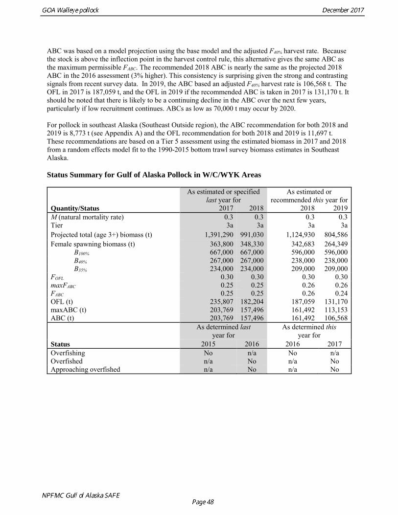
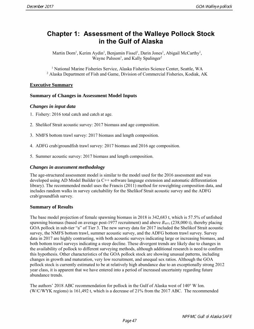
ABC was based on a model projection using the base model and the adjusted F40% harvest rate. Because the stock is above the inflection point in the harvest control rule, this alternative gives the same ABC as the maximum permissible FABC. The recommended 2018 ABC is nearly the same as the projected 2018 ABC in the 2016 assessment (3% higher). This consistency is surprising given the strong and contrasting signals from recent survey data. In 2019, the ABC based an adjusted F40% harvest rate is 106,568 t. The OFL in 2017 is 187,059 t, and the OFL in 2019 if the recommended ABC is taken in 2017 is 131,170 t. It should be noted that there is likely to be a continuing decline in the ABC over the next few years, particularly if low recruitment continues. ABCs as low as 70,000 t may occur by 2020. For pollock in southeast Alaska (Southeast Outside region), the ABC recommendation for both 2018 and 2019 is 8,773 t (see Appendix A) and the OFL recommendation for both 2018 and 2019 is 11,697 t. These recommendations are based on a Tier 5 assessment using the estimated biomass in 2017 and 2018 from a random effects model fit to the 1990-2015 bottom trawl survey biomass estimates in Southeast Alaska. Status Summary for Gulf of Alaska Pollock in W/C/WYK Areas

As estimated or specified

last year for As estimated or

recommended this year for Quantity/Status 2017 2018 2018 2019 M (natural mortality rate) 0.3 0.3 0.3 0.3 Tier 3a 3a 3a 3a Projected total (age 3+) biomass (t) 1,391,290 991,030 1,124,930 804,586 Female spawning biomass (t) 363,800 348,330 342,683 264,349 B100% 667,000 667,000 596,000 596,000 B40% 267,000 267,000 238,000 238,000 B35% 234,000 234,000 209,000 209,000 FOFL 0.30 0.30 0.30 0.30 maxFABC 0.25 0.25 0.26 0.26 FABC 0.25 0.25 0.26 0.24 OFL (t) 235,807 182,204 187,059 131,170 maxABC (t) 203,769 157,496 161,492 113,153 ABC (t) 203,769 157,496 161,492 106,568

Status

As determined last year for

As determined this year for

2015 2016 2016 2017 Overfishing No n/a No n/a Overfished n/a No n/a No Approaching overfished n/a No n/a No

Status Summary for Pollock in the Southeast Outside Area

Quantity

As estimated or specified last year for:

As estimated or recommended this year for:

2017 2018 2018 2019

M (natural mortality rate) 0.3 0.3 0.3 0.3 Tier 5 5 5 5 Biomass (t) Upper 95% confidence interval 76,781 83,089 70,502 75,820 Point estimate 44,087 44,087 38,989 38,989 Lower 95% confidence interval 25,315 23,393 21,562 20,050 FOFL 0.30 0.30 0.30 0.30 maxFABC 0.23 0.23 0.23 0.23 FABC 0.23 0.23 0.23 0.23 OFL (t) 13,226 13,226 11,697 11,697 maxABC (t) 9,920 9,920 8,773 8,773 ABC (t) 9,920 9,920 8,773 8,773

Status As determined last year for: As determined this year for:

2015 2016 2016 2017 Overfishing No n/a No n/a

Responses to SSC and Plan Team Comments in General The SSC in its December 2016 minutes continued to support a standard naming convention for different models presented in assessments. In this assessment, we used the naming convention supported by the SSC. The base model in last year’s assessment was model 16.2. The recommended base model in this assessment is model 17.2. Responses to SSC and Plan Team Comments Specific to this Assessment The GOA plan team recommended in its November 2016 minutes that the summary information on economic performance be included in future assessments. A section on the economic performance of the GOA pollock fishery is again included in the assessment. The GOA plan team recommended in its November 2016 minutes continued development of the ADFG survey delta-GLM model, examining interactions and the possible inclusion of environmental covariates. The delta-GLM model for the ADFG survey was included again included in the assessment. We were unable to explore interaction terms or environmental covariates in the model. The GOA plan team recommended in its November 2016 minutes an evaluation of prediction error of the weight-at-age random effects model. We compare the predictions from last year’s weight-at-age random effects model with this year’s estimates.

The GOA plan team recommended in its November 2016 minutes a coordinated evaluation of annual change in ADFG survey biomass estimates relative to the NMFS bottom trawl survey for both Pacific cod and walleye pollock. We were unable to conduct this evaluation. The SSC its December 2016 minutes noted that number of assessments are adopting the geostatistical approach for estimating survey biomass and its uncertainty. The SSC recommended further exploration of geostatistical estimates for GOA pollock. Work presented to the joint plan teams in September indicated the application of VAST models to Gulf of Alaska survey data was not straightforward, and that additional analyses were needed before being fully confident in the approach. We did not put forward a model in this assessment using the VAST approach pending additional analyses to be completed. The SSC its December 2016 minutes looked forward to suggestions for model improvement during the CIE review in 2017. The CIE review for GOA pollock took place on May 22-25, 2017. Reviews were generally supportive of the current approach for the GOA pollock assessment. We summarized the reviews for the GOA plan team in September, and are developing a written response to the review that includes a work plan for the GOA pollock assessment moving forward. We will provide this plan to the GOA Plan Team and the SSC for consideration next year.

Introduction Walleye pollock (Gadus chalcogrammus; hereafter referred to as pollock) is a semi-pelagic schooling fish widely distributed in the North Pacific Ocean. Pollock in the central and western Gulf of Alaska (GOA) are managed as a single stock independently of pollock in the Bering Sea and Aleutian Islands. The separation of pollock in Alaskan waters into eastern Bering Sea and Gulf of Alaska stocks is supported by analysis of larval drift patterns from spawning locations (Bailey et al. 1997), genetic studies of allozyme frequencies (Grant and Utter 1980), mtDNA variability (Mulligan et al. 1992), and microsatellite allele variability (Bailey et al. 1997). The results of studies of stock structure within the Gulf of Alaska are equivocal. There is evidence from allozyme frequency and mtDNA that spawning populations in the northern part of the Gulf of Alaska (Prince William Sound and Middleton Island) may be genetically distinct from the Shelikof Strait spawning population (Olsen et al. 2002). However significant variation in allozyme frequency was found between Prince William Sound samples in 1997 and 1998, indicating a lack of stability in genetic structure for this spawning population. Olsen et al. (2002) suggest that interannual genetic variation may be due to variable reproductive success, adult philopatry, source-sink population structure, or utilization of the same spawning areas by genetically distinct stocks with different spawning timing. An evaluation of stock structure for Gulf of Alaska pollock following the template developed by NPFMC stock structure working group was provided as an appendix to the 2012 assessment (Dorn et al., 2012). Available information supported the current approach of assessing and managing pollock in the eastern portion of the Gulf of Alaska (Southeast Outside) separately from pollock in the central and western portions of the Gulf of Alaska (Central/Western/West Yakutat). The main part of this assessment deals only with the C/W/WYK stock, while results for a tier 5 assessment for southeast outside pollock are reported in Appendix A. Fishery

The commercial fishery for walleye pollock in the Gulf of Alaska started as a foreign fishery in the early 1970s (Megrey 1989). Catches increased rapidly during the late 1970s and early 1980s (Table 1.1). A large spawning aggregation was discovered in Shelikof Strait in 1981, and a fishery developed for which pollock roe was an important product. The domestic fishery for pollock developed rapidly in the Gulf of Alaska with only a short period of joint venture operations in the mid-1980s. The fishery was fully domestic by 1988. The pollock target fishery in the Gulf of Alaska is entirely shore-based with approximately 90% of the catch taken with pelagic trawls. During winter, fishing effort targets pre-spawning aggregations in Shelikof Strait and near the Shumagin Islands (Fig. 1.1). Fishing in summer is less predictable, but typically occurs in deep-water troughs on the east side of Kodiak Island and along the Alaska Peninsula. Incidental catch in the Gulf of Alaska directed pollock fishery is low. For tows classified as pollock targets in the Gulf of Alaska between 2012 and 2016, on average about 96% of the catch by weight of FMP species consisted of pollock (Table 1.2). Nominal pollock targets are defined by the dominance of pollock in the catch, and may include tows where other species were targeted, but pollock were caught instead. The most common managed species in the incidental catch are arrowtooth flounder, Pacific cod, Pacific ocean perch, flathead sole, shallow-water flatfish, and squid. The most common non-target species are grenadiers, eulachon and other osmerids, miscellaneous fish, and jellyfish (Table 1.2). Bycatch estimates for prohibited species over the period 2012-2016 are given in Table 1.3. Chinook salmon are the most important prohibited species caught as bycatch in the pollock fishery. A sharp spike in Chinook salmon bycatch in 2010 led the Council to adopt management measures to reduce Chinook salmon

bycatch, including a cap of 25,000 Chinook salmon bycatch in directed pollock fishery. Estimated Chinook salmon bycatch since 2010 has been less than the peak in 2010, but increased in 2016. Since 1992, the Gulf of Alaska pollock Total Allowable Catch (TAC) has been apportioned spatially and temporally to reduce potential impacts on Steller sea lions. The details of the apportionment scheme have evolved over time, but the general objective is to allocate the TAC to management areas based on the distribution of surveyed biomass, and to establish three or four seasons between mid-January and fall during which some fraction of the TAC can be taken. The Steller Sea Lion Protection Measures implemented in 2001 established four seasons in the Central and Western GOA beginning January 20, March 10, August 25, and October 1, with 25% of the total TAC allocated to each season. Allocations to management areas 610, 620 and 630 are based on the seasonal biomass distribution as estimated by groundfish surveys. In addition, a harvest control rule was implemented that requires suspension of directed pollock fishing when spawning biomass declines below 20% of the reference unfished level. Data Used in the Assessment

The data used in the assessment model consist of estimates of annual catch in tons, fishery age composition, NMFS summer bottom trawl survey estimates of biomass and age composition, acoustic survey estimates of biomass and age composition in Shelikof Strait, summer acoustic survey estimates of biomass and age composition, and ADFG bottom trawl survey estimates of biomass and age composition. Binned length composition data are used in the model only when age composition estimates are unavailable, such as the most recent surveys. The following table specifies the data that were used in the GOA pollock assessment:

Source Data Years Fishery Total catch 1970-2016 Fishery Age composition 1975-2016 Shelikof Strait acoustic survey Biomass 1992-2017 Shelikof Strait acoustic survey Age composition 1992-2017 Summer acoustic survey Biomass 2013-2017 Summer acoustic survey Age composition 2013, 2015 Summer acoustic survey Length composition 2017 NMFS bottom trawl survey Area-swept biomass 1990-2017 NMFS bottom trawl survey Age composition 1990-2015 NMFS bottom trawl survey Length composition 2017 ADFG trawl survey Area-swept biomass 1989-2017 ADFG survey Age composition 2000-2016

Total Catch Total catch estimates were obtained from INPFC and ADFG publications, and databases maintained at the Alaska Fisheries Science Center and the Alaska Regional Office. Foreign catches for 1963-1970 are reported in Forrester et al. (1978). During this period only Japanese vessels reported catch of pollock in the GOA, though there may have been some catches by Soviet Union vessels. Foreign catches 1971-1976 are reported by Forrester et al. (1983). During this period there are reported pollock catches for Japanese, Soviet Union, Polish, and South Korean vessels in the Gulf of Alaska. Foreign and joint venture catches for 1977-1988 are blend estimates from the NORPAC database maintained by the Alaska Fisheries Science Center. Domestic catches for 1970-1980 are reported in Rigby (1984). Domestic catches for 1981-1990 were obtained from PacFIN (Brad Stenberg, pers. comm. Feb 7, 2014). A discard ratio (discard/retained) of 13.5% was assumed for all domestic catches prior to 1991 based on the 1991-1992

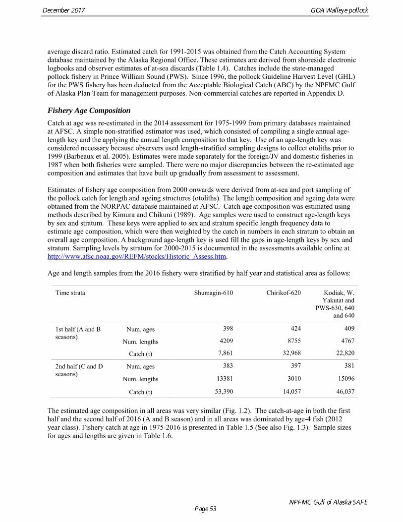
average discard ratio. Estimated catch for 1991-2015 was obtained from the Catch Accounting System database maintained by the Alaska Regional Office. These estimates are derived from shoreside electronic logbooks and observer estimates of at-sea discards (Table 1.4). Catches include the state-managed pollock fishery in Prince William Sound (PWS). Since 1996, the pollock Guideline Harvest Level (GHL) for the PWS fishery has been deducted from the Acceptable Biological Catch (ABC) by the NPFMC Gulf of Alaska Plan Team for management purposes. Non-commercial catches are reported in Appendix D. Fishery Age Composition Catch at age was re-estimated in the 2014 assessment for 1975-1999 from primary databases maintained at AFSC. A simple non-stratified estimator was used, which consisted of compiling a single annual age-length key and the applying the annual length composition to that key. Use of an age-length key was considered necessary because observers used length-stratified sampling designs to collect otoliths prior to 1999 (Barbeaux et al. 2005). Estimates were made separately for the foreign/JV and domestic fisheries in 1987 when both fisheries were sampled. There were no major discrepancies between the re-estimated age composition and estimates that have built up gradually from assessment to assessment. Estimates of fishery age composition from 2000 onwards were derived from at-sea and port sampling of the pollock catch for length and ageing structures (otoliths). The length composition and ageing data were obtained from the NORPAC database maintained at AFSC. Catch age composition was estimated using methods described by Kimura and Chikuni (1989). Age samples were used to construct age-length keys by sex and stratum. These keys were applied to sex and stratum specific length frequency data to estimate age composition, which were then weighted by the catch in numbers in each stratum to obtain an overall age composition. A background age-length key is used fill the gaps in age-length keys by sex and stratum. Sampling levels by stratum for 2000-2015 is documented in the assessments available online at http://www.afsc.noaa.gov/REFM/stocks/Historic_Assess.htm. Age and length samples from the 2016 fishery were stratified by half year and statistical area as follows:

Time strata Shumagin-610 Chirikof-620 Kodiak, W. Yakutat and

PWS-630, 640 and 640

1st half (A and B seasons)

Num. ages 398 424 409

Num. lengths 4209 8755 4767

Catch (t) 7,861 32,968 22,820

2nd half (C and D seasons)

Num. ages 383 397 381

Num. lengths 13381 3010 15096

Catch (t) 53,390 14,057 46,037

The estimated age composition in all areas was very similar (Fig. 1.2). The catch-at-age in both the first half and the second half of 2016 (A and B season) and in all areas was dominated by age-4 fish (2012 year class). Fishery catch at age in 1975-2016 is presented in Table 1.5 (See also Fig. 1.3). Sample sizes for ages and lengths are given in Table 1.6.

Gulf of Alaska Bottom Trawl Survey Trawl surveys have been conducted by Alaska Fisheries Science Center (AFSC) beginning in 1984 to assess the abundance of groundfish in the Gulf of Alaska (Table 1.7). Starting in 2001, the survey frequency was increased from once every three years to once every two years. The survey uses a stratified random design, with 49 strata based on depth, habitat, and statistical area (von Szalay et al. 2010). Area-swept biomass estimates are obtained using mean CPUE (standardized for trawling distance and mean net width) and stratum area. The survey is conducted from chartered commercial bottom trawlers using standardized poly-Nor‘eastern high opening bottom trawls rigged with roller gear. In a typical survey, 800 tows are completed. On average, 73% of these tows contain pollock (Table 1.8). The time series of pollock biomass used in the assessment model is based on the surveyed area in the Gulf of Alaska west of 140° W lon., obtained by adding the biomass estimates for the Shumagin-610, Chirikof-620, Kodiak-630 statistical areas, and the western portion of Yakutat-640 statistical area. Biomass estimates for the west Yakutat area were obtained by splitting strata and survey CPUE data at 140° W lon. and re-estimating biomass for west Yakutat. In 2001, when eastern Gulf of Alaska was not surveyed, a random effects model was used to interpolate a value for west Yakutat for use in the assessment model. The Alaska Fisheries Science Center’s (AFSC) Resource Assessment and Conservation Engineering (RACE) Division conducted the fifteenth comprehensive bottom trawl survey since 1984 during the summer of 2017 (Fig. 1.4). The 2017 gulfwide biomass estimate of pollock was 315,116 t, which is a decrease of 58% from the 2015 estimate, and is the second lowest in the time series after 2001. he biomass estimate for the portion of the Gulf of Alaska west of 140º W long. used in the assessment model is 288,943 t. The coefficient of variation (CV) of this estimate was 0.44, which makes it the most uncertain estimate in the times series. The CVs in the previous three surveys averaged 0.17. The increase in uncertainty may be partly due to lower survey effort (two boats were used instead of three, and the number of tows was reduced from 772 tows in 2015 to 536 in 2017, Table 1.8), but may also reflect the patchier distribution of pollock in 2017. Surveys from 1990 onwards are used in the assessment due to the difficulty in standardizing the surveys in 1984 and 1987, when Japanese vessels with different gear were used. in standardizing the surveys in 1984 and 1987, when Japanese vessels with different gear were used. Bottom Trawl Survey Age Composition Estimates of numbers at age from the bottom trawl survey are obtained from random otolith samples and length frequency samples (Table 1.9). Numbers at age are estimated by statistical area (Shumagin-610, Chirikof-620, Kodiak-630, Yakutat-640 and Southeastern-650) using a global age-length key, and CPUE-weighted length frequency data by statistical area (Fig. 1.5). The combined Shumagin, Chirikof and Kodiak age composition is used in the assessment model. Since ages are not available for the 2017 survey, length composition was used in the assessment model. Length composition in 2017 indicated the presence of two modes, a mode around 18 cm representing age-1 pollock and second mode around 43 cm representing primarily age-5 fish from the 2012 year. Age-1 pollock were increasingly dominant in the length composition as the survey proceeded from west to east, and were particularity abundant in Southeast area (Fig. 1.6). The overall abundance of age-1 pollock was approximately 460 million, with 51% of the total in the Southeast area. Shelikof Strait Acoustic Survey Winter acoustic surveys to assess the biomass of pre-spawning aggregations pollock in Shelikof Strait have been conducted annually since 1981 (except 1982, 1999, and 2011). Only surveys from 1992 and later are used in the stock assessment due to the higher uncertainty associated with the acoustic estimates produced with the Biosonics echosounder used prior to 1992. Additionally, raw survey data are not easily recoverable for the earlier acoustic surveys, so there is no way to verify (i.e., to reproduce) the estimates.

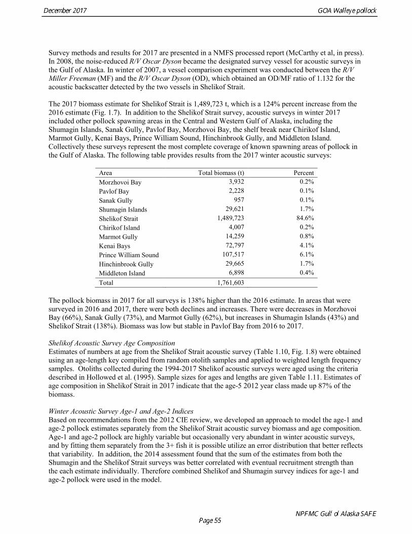
Survey methods and results for 2017 are presented in a NMFS processed report (McCarthy et al, in press). In 2008, the noise-reduced R/V Oscar Dyson became the designated survey vessel for acoustic surveys in the Gulf of Alaska. In winter of 2007, a vessel comparison experiment was conducted between the R/V Miller Freeman (MF) and the R/V Oscar Dyson (OD), which obtained an OD/MF ratio of 1.132 for the acoustic backscatter detected by the two vessels in Shelikof Strait. The 2017 biomass estimate for Shelikof Strait is 1,489,723 t, which is a 124% percent increase from the 2016 estimate (Fig. 1.7). In addition to the Shelikof Strait survey, acoustic surveys in winter 2017 included other pollock spawning areas in the Central and Western Gulf of Alaska, including the Shumagin Islands, Sanak Gully, Pavlof Bay, Morzhovoi Bay, the shelf break near Chirikof Island, Marmot Gully, Kenai Bays, Prince William Sound, Hinchinbrook Gully, and Middleton Island. Collectively these surveys represent the most complete coverage of known spawning areas of pollock in the Gulf of Alaska. The following table provides results from the 2017 winter acoustic surveys:

Area Total biomass (t) Percent Morzhovoi Bay 3,932 0.2% Pavlof Bay 2,228 0.1% Sanak Gully 957 0.1% Shumagin Islands 29,621 1.7% Shelikof Strait 1,489,723 84.6% Chirikof Island 4,007 0.2% Marmot Gully 14,259 0.8% Kenai Bays 72,797 4.1% Prince William Sound 107,517 6.1% Hinchinbrook Gully 29,665 1.7% Middleton Island 6,898 0.4% Total 1,761,603

The pollock biomass in 2017 for all surveys is 138% higher than the 2016 estimate. In areas that were surveyed in 2016 and 2017, there were both declines and increases. There were decreases in Morzhovoi Bay (66%), Sanak Gully (73%), and Marmot Gully (62%), but increases in Shumagin Islands (43%) and Shelikof Strait (138%). Biomass was low but stable in Pavlof Bay from 2016 to 2017. Shelikof Acoustic Survey Age Composition Estimates of numbers at age from the Shelikof Strait acoustic survey (Table 1.10, Fig. 1.8) were obtained using an age-length key compiled from random otolith samples and applied to weighted length frequency samples. Otoliths collected during the 1994-2017 Shelikof acoustic surveys were aged using the criteria described in Hollowed et al. (1995). Sample sizes for ages and lengths are given Table 1.11. Estimates of age composition in Shelikof Strait in 2017 indicate that the age-5 2012 year class made up 87% of the biomass. Winter Acoustic Survey Age-1 and Age-2 Indices Based on recommendations from the 2012 CIE review, we developed an approach to model the age-1 and age-2 pollock estimates separately from the Shelikof Strait acoustic survey biomass and age composition. Age-1 and age-2 pollock are highly variable but occasionally very abundant in winter acoustic surveys, and by fitting them separately from the 3+ fish it is possible utilize an error distribution that better reflects that variability. In addition, the 2014 assessment found that the sum of the estimates from both the Shumagin and the Shelikof Strait surveys was better correlated with eventual recruitment strength than the each estimate individually. Therefore combined Shelikof and Shumagin survey indices for age-1 and age-2 pollock were used in the model.

Summer Acoustic Survey Three complete acoustic surveys, in 2013, 2015, 2017, have been conducted by AFSC on the R/V Oscar Dyson in the Gulf of Alaska during summer (Jones et al. 2014, Jones et al. in prep.). The area surveyed covers the Gulf of Alaska shelf and upper slope, and extends eastward to 140° W lon. Prince William Sound is also surveyed. In 2017, nearshore survey transects in Izhut Bay, Kenai Bays and Prince William Sound were cancelled due to equipment breakdown and repair on the R/V Oscar Dyson, but these areas accounted less than 2% of the total biomass in 2013 and 2015. The survey consists of widely-spaced parallel transects along the shelf, and more closely spaced transects in troughs, bays, and Shelikof Strait. Mid-water and bottom trawls are used to identify acoustic targets. Size composition in 2017 indicated that the very abundant 2012 year class (age-5 fish) was dominant, though a secondary mode of age-1 pollock (15-25 cm) was present in the central GOA (Fig. 1.9). The estimate of pollock biomass for the 2017 survey was 1,318,396 t, a decrease of 18% from the 2015 survey. Analysis of the 2017 survey was complicated by the presence of age-0 pollock, which were very abundant, widely-distributed, and mixed with juvenile and adult pollock backscatter. Since both the summer bottom trawl and summer acoustic surveys are conducted from west to east on roughly a similar timetable, methods described by Kotwicki et al. (2017) could be applied to combine data from both surveys. Alaska Department of Fish and Game Crab/Groundfish Trawl Survey The Alaska Department of Fish and Game (ADFG) has conducted bottom trawl surveys of nearshore areas of the Gulf of Alaska since 1987. Although these surveys are designed to monitor population trends of Tanner crab and red king crab, pollock and other fish are also sampled. Standardized survey methods using a 400-mesh eastern trawl were employed from 1987 to the present. The survey is designed to sample at fixed stations from mostly nearshore areas from Kodiak Island to Unimak Pass, and does not cover the entire shelf area (Fig. 1.10). The average number of tows completed during the survey is 360. On average, 86% of these tows contain pollock. Details of the ADFG trawl gear and sampling procedures are in Spalinger (2012). The 2017 area-swept biomass estimate for pollock for the ADFG crab/groundfish survey was 21,855 t, up 18% from the 2016 biomass estimate, which was the lowest biomass in the ADFG crab/groundfish time series (Table 1.7). This indicates that the recent pollock estimates for this survey continue remain at very low levels relative to historical levels. Delta GLM indices A simple delta GLM model was applied to the ADFG tow by tow data for 1988-2017 to obtain annual abundance indices. Data were filtered to exclude missing latitude and longitudes (1 tow) and missing depths (4 tows). Tows made in lower Shelikof Strait (between 154.7° W lon. and 156.7° W lon.) were excluded because these stations were occupied irregularly (157 tows). The delta GLM model fit a separate model to the presence-absence observations and to the positive observations. A fixed effects model was used with the year, geographic area, and depth as factors. Strata were defined according to ADFG district (Kodiak, Chignik, South Peninsula) and depth (<30 fm, 30-100 fm, >100 fm). Alternative depth strata were evaluated, and model results were found to be robust to different depth strata assumptions. The same model structure was used for both the presence-absence observations and the positive observations. The error assumption of presence-absence observations was assumed to be binomial, and, as usual, several alternative error assumptions were evaluated for the positive observations, including lognormal, gamma, and inverse Gaussian. The inverse Gaussian model did not converge, and AIC statistic strongly indicated the gamma distribution was more appropriate than the lognormal (ΔAIC= 494.2). A quantile-quantile plot for the gamma model residuals was not ideal, but was considered acceptable (Fig. 1.11). Comparison of delta-GLM indices the area-swept estimates indicated similar trends (Fig. 1.12). Variances were based on a bootstrap procedure, and CVs for the annual index ranged from 0.09 to 0.20. These values understate

the uncertainty of the indices with respect to population trends, since the area covered by the survey is a relatively small percentage of the GOA shelf area. ADFG Survey Age Composition Ages were determined by age readers in the AFSC age and growth unit from samples of pollock otoliths collected during 2000-2016 ADFG surveys in even-numbered years (average sample size = 580) (Table 1.12, Fig. 1.13). Comparison with fishery age composition shows that older fish (> age-8) are more common in the ADFG crab/groundfish survey. This is consistent with the assessment model, which estimates a domed-shaped selectivity pattern for the fishery, but an asymptotic selectivity pattern for the ADFG survey. Data sets considered but not used Egg Production Estimates of Spawning Biomass Estimates of spawning biomass in Shelikof Strait based on egg production methods were produced during 1981-92 (Table 1.7). A complete description of the estimation process is given in Picquelle and Megrey (1993). Egg production estimates were discontinued in 1992 because the Shelikof Strait acoustic survey provided similar information. The egg production estimates are not used in the assessment model because the surveys are no longer being conducted, and because the acoustic surveys in Shelikof Strait show a similar trend over the period when both were conducted. Pre-1984 bottom trawl surveys Considerable survey work was carried out in the Gulf of Alaska prior to the start of the NMFS triennial bottom trawl surveys in 1984. Between 1961 and the mid-1980s, the most common bottom trawl used for surveying was the 400-mesh eastern trawl. This trawl (or variants thereof) was used by IPHC for juvenile halibut surveys in the 1960s, 1970s, and early 1980s, and by NMFS for groundfish surveys in the 1970s. Von Szalay and Brown (2001) estimated a fishing power correction (FPC) for the ADFG 400-mesh eastern trawl of 3.84 (SE = 1.26), indicating that 400-mesh eastern trawl CPUE for pollock would need to be multiplied by this factor to be comparable to the NMFS poly-Nor’eastern trawl. In most cases, earlier surveys in the Gulf of Alaska were not designed to be comprehensive, with the general strategy being to cover the Gulf of Alaska west of Cape Spencer over a period of years, or to survey a large area to obtain an index for group of groundfish, i.e., flatfish or rockfish. For example, Ronholt et al. (1978) combined surveys for several years to obtain gulfwide estimates of pollock biomass for 1973-6. There are several difficulties with such an approach, including the possibility of double-counting or missing a portion of the stock that happened to migrate between surveyed areas. Due to the difficulty in constructing a consistent time series, the historical survey estimates are no longer used in the assessment model. Multi-year combined survey estimates indicate a large increase in pollock biomass in the Gulf of Alaska occurred between the early 1960s and the mid 1970s. Increases in pollock biomass between the1960s and 1970s were also noted by Alton et al. (1987). In the 1961 survey, pollock were a relatively minor component of the groundfish community with a mean CPUE of 16 kg/hr. (Ronholt et al. 1978). Arrowtooth flounder was the most common groundfish with a mean CPUE of 91 kg/hr. In the 1973-76 surveys, the CPUE of arrowtooth flounder was similar to the 1961 survey (83 kg/hr.), but pollock CPUE had increased 20-fold to 321 kg/hr., and was by far the dominant groundfish species in the Gulf of Alaska. Mueter and Norcross (2002) also found that pollock was low in the relative abundance in 1960s, became the dominant species in Gulf of Alaska groundfish community in the 1970s, and subsequently declined in relative abundance.

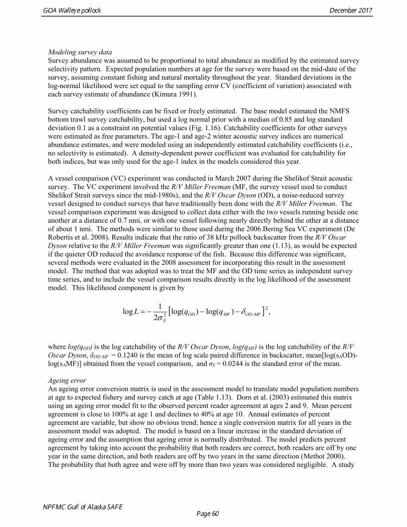
Questions concerning the comparability of pollock CPUE data from historical trawl surveys with later surveys probably can never be fully resolved. However, because of the large magnitude of the change in CPUE between the surveys in the 1960s and the early 1970s using similar trawling gear, the conclusion that there was a large increase in pollock biomass seems robust. Early speculation about the rise of pollock in the Gulf of Alaska in the early 1970s implicated the large biomass removals of Pacific ocean perch, a potential competitor for euphausid prey (Somerton 1979, Alton et al. 1987). More recent work has focused on role of climate change (Anderson and Piatt 1999, Bailey 2000). These earlier surveys suggest that population biomass in the 1960s, prior to large-scale commercial exploitation of the stock, may have been lower than at any time since then. Qualitative trends To assess qualitatively recent trends in abundance, each survey time series was standardized by dividing the annual estimate by the average since 1990. Shelikof Strait acoustic survey estimates prior to 2008 were rescaled to be comparable to subsequent surveys conducted by the R/V Oscar Dyson. Although there is considerable variability in each survey time series, a fairly clear downward trend is evident to 2000, followed by a stable, though variable, trend to 2008, followed by a strong increase to 2013 (Fig. 1.14). In last few years there has been strong divergence the trends, particularly in 2017. Both the ADFG and the bottom trawl surveys indicate a steep decline in abundance, while the Shelikof Strait acoustic survey in 2017 increase to more than twice the long-term average. Indices derived from fisheries catch data were also evaluated for trends in biological characteristics (Fig. 1.15). The percent of females in the catch shows some variability but no obvious trend, and is usually close to 50-50. In 2016, the percent female dropped to 40%. Evaluation of sex ratios by season indicated that this decrease was mostly due a very low percentage of females during the A and B seasons prior to spawning. However the sex ratio during the C and D seasons was close to 50-50, suggesting the skewed sex in winter was related to spawning behavior, rather than an indication of a population characteristic. The mean age shows interannual variability due to strong year classes passing through the population, but there are no downward trends that would suggest excessive mortality rates. The percent of old fish in the catch (nominally defined as age 8 and older) is also highly variable due to variability in year class strength. The percent of old fish declined in 2015 and 2016 as the strong 2012 year class recruited to the fishery. Under a constant F40% harvest rate, the mean percent of age 8 and older fish in the catch is approximately 8%. An index of catch at age diversity was computed using the Shannon-Wiener information index, where pa is the proportion at age. Increases in fishing mortality would tend to reduce age diversity, but year class variability would also influence age diversity. The index of age diversity is relatively stable during 1975-2015, but declined sharply in 2017 due to the dominance of the 2012 year class in the catch (Fig. 1.15). A remarkable number of indicators that showed unusual values in 2017, which raises some concern, though the implications for pollock population dynamics are unclear. Analytic Approach

Model Structure An age-structured model covering the period from 1970 to 2017 (48 years) was used to assess Gulf of Alaska pollock. The modeled population includes individuals from age 1 to age 10, with age 10 defined as a “plus” group, i.e., all individuals age 10 and older. Population dynamics were modeled using standard formulations for mortality and fishery catch (e.g. Fournier and Archibald 1982, Deriso et al. 1985, Hilborn and Walters 1992). Year- and age-specific fishing mortality was modeled as a product of a

− ∑ p pa aln ,

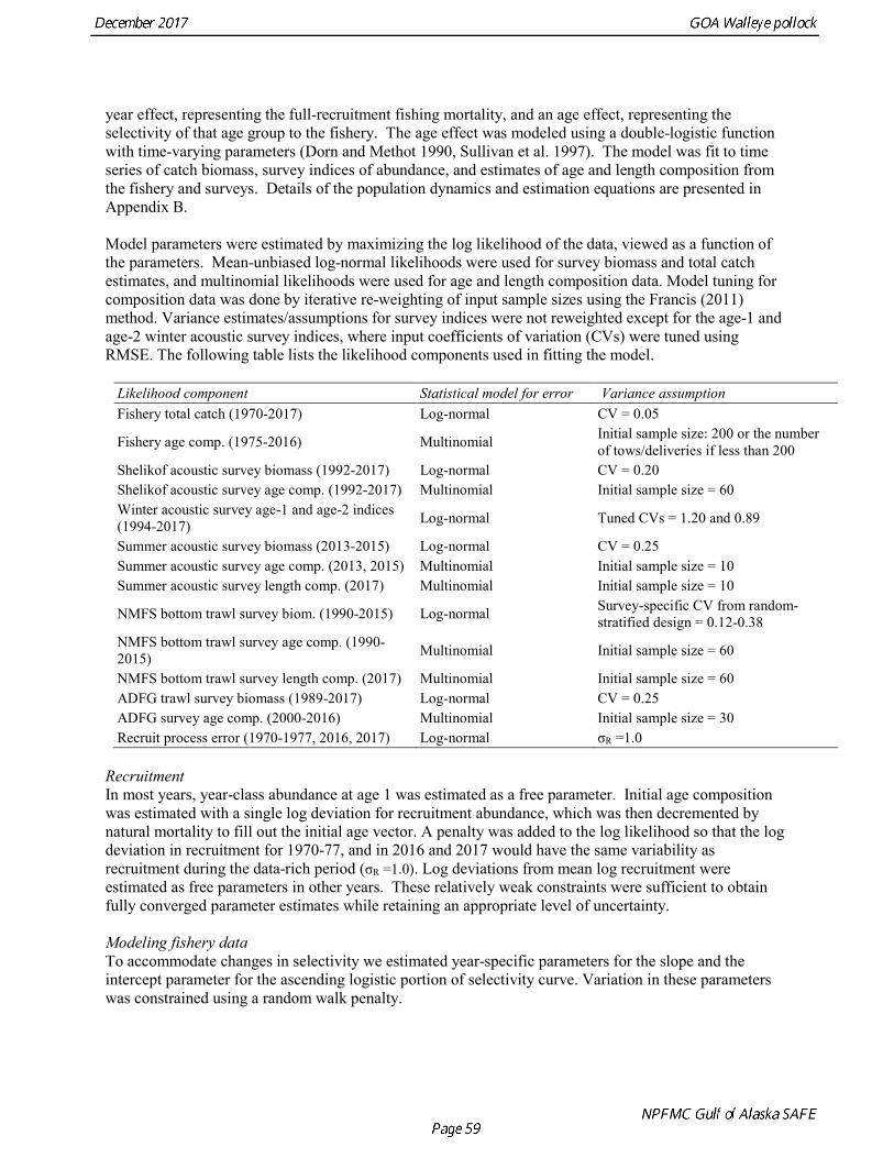
year effect, representing the full-recruitment fishing mortality, and an age effect, representing the selectivity of that age group to the fishery. The age effect was modeled using a double-logistic function with time-varying parameters (Dorn and Methot 1990, Sullivan et al. 1997). The model was fit to time series of catch biomass, survey indices of abundance, and estimates of age and length composition from the fishery and surveys. Details of the population dynamics and estimation equations are presented in Appendix B. Model parameters were estimated by maximizing the log likelihood of the data, viewed as a function of the parameters. Mean-unbiased log-normal likelihoods were used for survey biomass and total catch estimates, and multinomial likelihoods were used for age and length composition data. Model tuning for composition data was done by iterative re-weighting of input sample sizes using the Francis (2011) method. Variance estimates/assumptions for survey indices were not reweighted except for the age-1 and age-2 winter acoustic survey indices, where input coefficients of variation (CVs) were tuned using RMSE. The following table lists the likelihood components used in fitting the model.

Likelihood component Statistical model for error Variance assumption Fishery total catch (1970-2017) Log-normal CV = 0.05

Fishery age comp. (1975-2016) Multinomial Initial sample size: 200 or the number of tows/deliveries if less than 200

Shelikof acoustic survey biomass (1992-2017) Log-normal CV = 0.20 Shelikof acoustic survey age comp. (1992-2017) Multinomial Initial sample size = 60 Winter acoustic survey age-1 and age-2 indices (1994-2017) Log-normal Tuned CVs = 1.20 and 0.89

Summer acoustic survey biomass (2013-2015) Log-normal CV = 0.25 Summer acoustic survey age comp. (2013, 2015) Multinomial Initial sample size = 10 Summer acoustic survey length comp. (2017) Multinomial Initial sample size = 10

NMFS bottom trawl survey biom. (1990-2015) Log-normal Survey-specific CV from random-stratified design = 0.12-0.38

NMFS bottom trawl survey age comp. (1990-2015) Multinomial Initial sample size = 60

NMFS bottom trawl survey length comp. (2017) Multinomial Initial sample size = 60 ADFG trawl survey biomass (1989-2017) Log-normal CV = 0.25 ADFG survey age comp. (2000-2016) Multinomial Initial sample size = 30 Recruit process error (1970-1977, 2016, 2017) Log-normal σR =1.0

Recruitment In most years, year-class abundance at age 1 was estimated as a free parameter. Initial age composition was estimated with a single log deviation for recruitment abundance, which was then decremented by natural mortality to fill out the initial age vector. A penalty was added to the log likelihood so that the log deviation in recruitment for 1970-77, and in 2016 and 2017 would have the same variability as recruitment during the data-rich period (σR =1.0). Log deviations from mean log recruitment were estimated as free parameters in other years. These relatively weak constraints were sufficient to obtain fully converged parameter estimates while retaining an appropriate level of uncertainty. Modeling fishery data To accommodate changes in selectivity we estimated year-specific parameters for the slope and the intercept parameter for the ascending logistic portion of selectivity curve. Variation in these parameters was constrained using a random walk penalty.

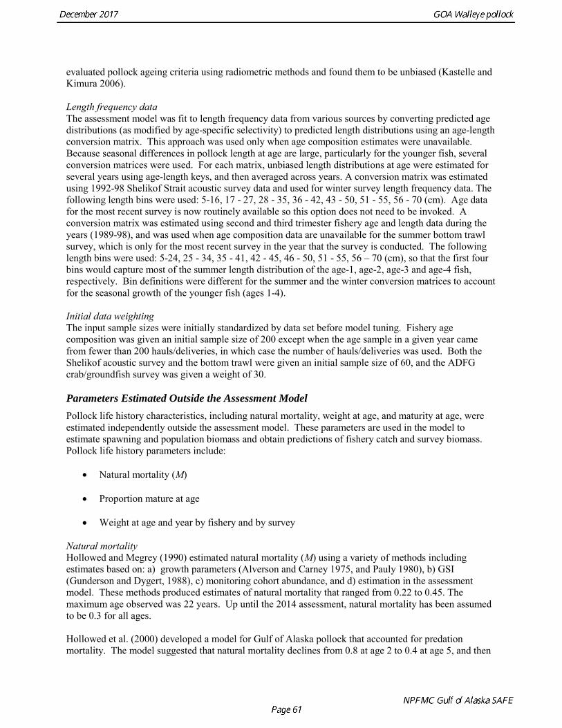
Modeling survey data Survey abundance was assumed to be proportional to total abundance as modified by the estimated survey selectivity pattern. Expected population numbers at age for the survey were based on the mid-date of the survey, assuming constant fishing and natural mortality throughout the year. Standard deviations in the log-normal likelihood were set equal to the sampling error CV (coefficient of variation) associated with each survey estimate of abundance (Kimura 1991). Survey catchability coefficients can be fixed or freely estimated. The base model estimated the NMFS bottom trawl survey catchability, but used a log normal prior with a median of 0.85 and log standard deviation 0.1 as a constraint on potential values (Fig. 1.16). Catchability coefficients for other surveys were estimated as free parameters. The age-1 and age-2 winter acoustic survey indices are numerical abundance estimates, and were modeled using an independently estimated catchability coefficients (i.e., no selectivity is estimated). A density-dependent power coefficient was evaluated for catchability for both indices, but was only used for the age-1 index in the models considered this year. A vessel comparison (VC) experiment was conducted in March 2007 during the Shelikof Strait acoustic survey. The VC experiment involved the R/V Miller Freeman (MF, the survey vessel used to conduct Shelikof Strait surveys since the mid-1980s), and the R/V Oscar Dyson (OD), a noise-reduced survey vessel designed to conduct surveys that have traditionally been done with the R/V Miller Freeman. The vessel comparison experiment was designed to collect data either with the two vessels running beside one another at a distance of 0.7 nmi, or with one vessel following nearly directly behind the other at a distance of about 1 nmi. The methods were similar to those used during the 2006 Bering Sea VC experiment (De Robertis et al. 2008). Results indicate that the ratio of 38 kHz pollock backscatter from the R/V Oscar Dyson relative to the R/V Miller Freeman was significantly greater than one (1.13), as would be expected if the quieter OD reduced the avoidance response of the fish. Because this difference was significant, several methods were evaluated in the 2008 assessment for incorporating this result in the assessment model. The method that was adopted was to treat the MF and the OD time series as independent survey time series, and to include the vessel comparison results directly in the log likelihood of the assessment model. This likelihood component is given by where log(qOD) is the log catchability of the R/V Oscar Dyson, log(qMF) is the log catchability of the R/V Oscar Dyson, δOD:MF = 0.1240 is the mean of log scale paired difference in backscatter, mean[log(sAOD)-log(sAMF)] obtained from the vessel comparison, and σS = 0.0244 is the standard error of the mean. Ageing error An ageing error conversion matrix is used in the assessment model to translate model population numbers at age to expected fishery and survey catch at age (Table 1.13). Dorn et al. (2003) estimated this matrix using an ageing error model fit to the observed percent reader agreement at ages 2 and 9. Mean percent agreement is close to 100% at age 1 and declines to 40% at age 10. Annual estimates of percent agreement are variable, but show no obvious trend; hence a single conversion matrix for all years in the assessment model was adopted. The model is based on a linear increase in the standard deviation of ageing error and the assumption that ageing error is normally distributed. The model predicts percent agreement by taking into account the probability that both readers are correct, both readers are off by one year in the same direction, and both readers are off by two years in the same direction (Methot 2000). The probability that both agree and were off by more than two years was considered negligible. A study

[ ] ,)log()log(2

1log 2:2 MFODMFOD

S

qqL δσ

−−−=

evaluated pollock ageing criteria using radiometric methods and found them to be unbiased (Kastelle and Kimura 2006). Length frequency data The assessment model was fit to length frequency data from various sources by converting predicted age distributions (as modified by age-specific selectivity) to predicted length distributions using an age-length conversion matrix. This approach was used only when age composition estimates were unavailable. Because seasonal differences in pollock length at age are large, particularly for the younger fish, several conversion matrices were used. For each matrix, unbiased length distributions at age were estimated for several years using age-length keys, and then averaged across years. A conversion matrix was estimated using 1992-98 Shelikof Strait acoustic survey data and used for winter survey length frequency data. The following length bins were used: 5-16, 17 - 27, 28 - 35, 36 - 42, 43 - 50, 51 - 55, 56 - 70 (cm). Age data for the most recent survey is now routinely available so this option does not need to be invoked. A conversion matrix was estimated using second and third trimester fishery age and length data during the years (1989-98), and was used when age composition data are unavailable for the summer bottom trawl survey, which is only for the most recent survey in the year that the survey is conducted. The following length bins were used: 5-24, 25 - 34, 35 - 41, 42 - 45, 46 - 50, 51 - 55, 56 – 70 (cm), so that the first four bins would capture most of the summer length distribution of the age-1, age-2, age-3 and age-4 fish, respectively. Bin definitions were different for the summer and the winter conversion matrices to account for the seasonal growth of the younger fish (ages 1-4). Initial data weighting The input sample sizes were initially standardized by data set before model tuning. Fishery age composition was given an initial sample size of 200 except when the age sample in a given year came from fewer than 200 hauls/deliveries, in which case the number of hauls/deliveries was used. Both the Shelikof acoustic survey and the bottom trawl were given an initial sample size of 60, and the ADFG crab/groundfish survey was given a weight of 30.

Parameters Estimated Outside the Assessment Model Pollock life history characteristics, including natural mortality, weight at age, and maturity at age, were estimated independently outside the assessment model. These parameters are used in the model to estimate spawning and population biomass and obtain predictions of fishery catch and survey biomass. Pollock life history parameters include:

• Natural mortality (M) • Proportion mature at age

• Weight at age and year by fishery and by survey

Natural mortality Hollowed and Megrey (1990) estimated natural mortality (M) using a variety of methods including estimates based on: a) growth parameters (Alverson and Carney 1975, and Pauly 1980), b) GSI (Gunderson and Dygert, 1988), c) monitoring cohort abundance, and d) estimation in the assessment model. These methods produced estimates of natural mortality that ranged from 0.22 to 0.45. The maximum age observed was 22 years. Up until the 2014 assessment, natural mortality has been assumed to be 0.3 for all ages. Hollowed et al. (2000) developed a model for Gulf of Alaska pollock that accounted for predation mortality. The model suggested that natural mortality declines from 0.8 at age 2 to 0.4 at age 5, and then

remains relatively stable with increasing age. In addition, stock size was higher when predation mortality was included. In a simulation study, Clark (1999) evaluated the effect of an erroneous M on both estimated abundance and target harvest rates for a simple age-structured model. He found that “errors in estimated abundance and target harvest rate were always in the same direction, with the result that, in the short term, extremely high exploitation rates can be recommended (unintentionally) in cases where the natural mortality rate is overestimated and historical exploitation rates in the catch-at-age data are low.” Clark (1999) proposed that the chance of this occurring could be reduced by using an estimate of natural mortality on the lower end of the credible range, which is the approach used in this assessment. In the 2014 assessment, several methods to estimate of the age-specific pattern of natural mortality were evaluated. Two general types of methods were used, both of which are external to the assessment model. The first type of method is based initially on theoretical life history or ecological relationships that are then evaluated using meta-analysis, resulting in an empirical equation that relates natural mortality to some more easily measured quantity such as length or weight. The second type of method is an age-structured statistical analysis using a multispecies model or single species model where predation is modeled. There are three examples of such models for pollock in Gulf of Alaska, a single species model with predation by Hollowed et al. (2000), and two multispecies models that included pollock by Van Kirk et al. (2010 and 2012). These models were published in the peer-reviewed literature, but likely did not receive the same level of scrutiny as stock assessment models. Although these models also estimate time-varying mortality, we averaged the total mortality (residual natural mortality plus predation mortality) for the last decade in the model to obtain a mean age-specific pattern (in some cases omitting the final year when estimates were much different than previous years). Use of the last decade was an attempt to use estimates with the strongest support from the data. Approaches for inclusion of time-varying natural mortality will be considered in future pollock assessments. The three theoretical/empirical methods used were the following: Brodziak et al. 2011—Age-specific M is given by 

𝑀𝑀(𝑎𝑎) = �𝑀𝑀𝑐𝑐𝐿𝐿𝑚𝑚𝑎𝑎𝑚𝑚𝐿𝐿(𝑎𝑎) 𝑓𝑓𝑓𝑓𝑓𝑓 𝑎𝑎 < 𝑎𝑎𝑚𝑚𝑎𝑎𝑚𝑚

𝑀𝑀𝑐𝑐 𝑓𝑓𝑓𝑓𝑓𝑓 𝑎𝑎 ≥ 𝑎𝑎𝑚𝑚𝑎𝑎𝑚𝑚 ,�

 where Lmat is the length at maturity, Mc = 0.30 is the natural mortality at Lmat, L(a) is mean length at age for the summer bottom trawl survey for 1984-2013.

Lorenzen 1996—Age-specific M for ocean ecosystems is given by

𝑀𝑀(𝑎𝑎) = 3.69 𝑊𝑊�𝑎𝑎 ,−0.305

where𝑊𝑊�𝑎𝑎is the mean weight at age from the summer bottom trawl survey for 1984-2013.is the mean weight at age from the summer bottom trawl survey for 1984-2013.

Gislason et al. 2010—Age-specific M is given by

ln(𝑀𝑀) = 0.55− 1.61 ln(𝐿𝐿) + 1.44 ln(𝐿𝐿∞) + ln(𝐾𝐾),

where L∞ = 65.2 cm and K = 0.30 were estimated by fitting von Bertalanffy growth curves using the NLS routine in R using summer bottom trawl age data for 2005-2009 for sexes combined in the central and western Gulf of Alaska.

Results were reasonably consistent and suggest use of a higher mortality rate for age classes younger than the age at maturity (Table 1.14 and Fig. 1.17). Somewhat surprisingly the theoretical/empirical estimates were similar on average to predation model estimates. To obtain an age-specific natural mortality schedule for use in the stock assessment, we used an ensemble approach and averaged the results for all methods. Then we used the method recommended by Clay Porch in Brodziak et al (2011) to rescale the age-specific values so that the average for range of ages equals a specified value. Age-specific values were rescaled so that a natural mortality for fish greater than or equal to age 5, the age at 50% maturity, was equal to 0.3, the value of natural mortality used in previous pollock assessments. Maturity at age Maturity stages for female pollock describe a continuous process of ovarian development between immature and post-spawning. For the purposes of estimating a maturity vector (the proportion of an age group that has been or will be reproductively active during the year) for stock assessment, all fish greater than or equal to a particular maturity stage are assumed to be mature, while those less than that stage are assumed to be immature. Maturity stages in which ovarian development had progressed to the point where ova were distinctly visible were assumed to be mature (i.e., stage 3 in the 5-stage pollock maturity scale). Maturity stages are qualitative rather than quantitative, so there is subjectivity in assigning stages, and a potential for different technicians to apply criteria differently (Neidetcher et al. 2014). Because the link between pre-spawning maturity stages and eventual reproductive activity later in the season is not well established, the division between mature and immature stages is problematic. Changes in the timing of spawning could also affect maturity at age estimates. Merati (1993) compared visual maturity stages with ovary histology and a blood assay for vitellogenin and found general consistency between the different approaches. Merati (1993) noted that ovaries classified as late developing stage (i.e., immature) may contain yolked eggs, but it was unclear whether these fish would have spawned later in the year. The average sample size of female pollock maturity stage data per year since 2000 from winter acoustic surveys in the Gulf of Alaska is 378 (Table 1.15). Estimates of maturity at age in 2016 from winter acoustic surveys substantially above the long term mean for all ages (Fig. 1.18), though except for the age-5 females from the 2012 year class the sample sizes were small and the estimates should not be considered reliable. Inter-annual changes in maturity at age may reflect environmental conditions, pollock population biology, effect of strong year classes moving through the population, or simply ageing error. Because there did not appear to be an objective basis for excluding data, the 1983-2017 average maturity at age was used in the assessment. Logistic regression (McCullagh and Nelder 1983) was also used to estimate the age and length at 50% maturity at age for each year to evaluate long-term changes in maturation. Annual estimates of age at 50% maturity are highly variable and range from 2.5 years in 1983 to 6.1 years in 1991, with an average of 4.8 years. The last few years has shown a decrease in the age at 50% mature, which is largely being driven by the maturation of 2012 years at younger ages than is typical. Length at 50% mature is less variable than the age at 50% mature, suggesting that at least some of the variability in the age at maturity can be attributed to changes in length at age (Fig 1.19). Changes in year-class dominance could also potentially affect estimates of maturity at age. There is less evidence of trends in the length at 50% mature, with the 1983 and 1984 estimates as unusually low values, the last few years showing a decline in the length at 50%. The average length at 50% mature for all years is approximately 43 cm.

Weight at age Year-specific weight-at-age estimates are used in the model to obtain expected catches in biomass. Where possible, year and survey-specific weight-at-age estimates are used to obtain expected survey biomass. For each data source, unbiased estimates of length at age were obtained using year-specific age-length keys. Bias-corrected parameters for the length-weight relationship,W a Lb= , were also estimated. Weights at age were estimated by multiplying length at age by the predicted weight based on the length-weight regressions. Weight at age for the fishery, the Shelikof Strait acoustic survey, and the NMFS bottom trawl survey are given in Table 1.16, Table 1.17, and Table 1.18, respectively. A plot of weight-at-age from the Shelikof Strait acoustic survey indicates that there has been a substantial increase in weight at age for older pollock (Fig. 1.20). For pollock greater than age 6, weight-at-age has nearly doubled since 1983-1990. However, weight at age in the last five years, 2012-2016, has been stable to decreasing, with a strong decline in the last three years. Further analyses are needed to evaluate whether these changes are a density-dependent response to declining pollock abundance, or whether they are environmentally forced. Changes in weight-at-age have potential implications for status determination and harvest control rules. A random effects (RE) model for weight at age (Ianelli et al. 2016) was used to improve estimates of fishery weight at age, and to propagate the uncertainty of weight at age when doing catch projections. The structural part of the model is an underlying von Bertalanffy growth curve. Year and cohort effects are estimated as random effects using the ADMB RE module. Further details are provided in Ianelli et al. (2016). Input data included fishery weight age for 1975-2016. The model also incorporates survey data by modeling an offset between fishery and survey weight at age. Weight at age for the Shelikof Strait acoustic survey (1981-2017) and the NMFS bottom trawl survey (1984-2015) were used. The model also requires input standard deviations for the weight at age data, which are not available for GOA pollock. In the 2006 assessment, a generalized variance function was developed using a quadratic curve to match the mean standard deviations at ages 3-10 for the eastern Bering Sea pollock data. The standard deviation at age one was assumed to be equal to the standard deviation at age 10. Survey weights at age were assumed to have standard deviations that were 1.5 times the fishery weights at age. A comparison of RE model estimates from last year of the 2016 fishery weight at age with the data now available indicate that the model tended to under-predict the weight at age for younger fish and over-predict the weight at age for older pollock (Fig. 1.21). However there was good agreement for age-4 pollock, which made up 86% of the catch at age. In this assessment, RE model estimates of weight at age are used for the fishery in 2017, and yield projections and spawning biomass per recruit calculations used the RE model estimates for 2018 (Fig. 1.21).

Parameters Estimated Inside the Assessment Model A large number of parameters are estimated when using this modeling approach, though many are year-specific deviations in fishery selectivity coefficients. Parameters were estimated using AD Model Builder (Version 10.1), a C++ software language extension and automatic differentiation library (Fournier et al. 2012). Parameters in nonlinear models are estimated in ADModel Builder using automatic differentiation software extended from Greiwank and Corliss (1991) and developed into C++ class libraries. The optimizer in AD Model Builder is a quasi-Newton routine (Press et al. 1992). The model is determined to have converged when the maximum parameter gradient is less than a small constant (set to 1 x 10-6). AD Model Builder includes post-convergence routines to calculate standard errors (or likelihood profiles) for any quantity of interest.

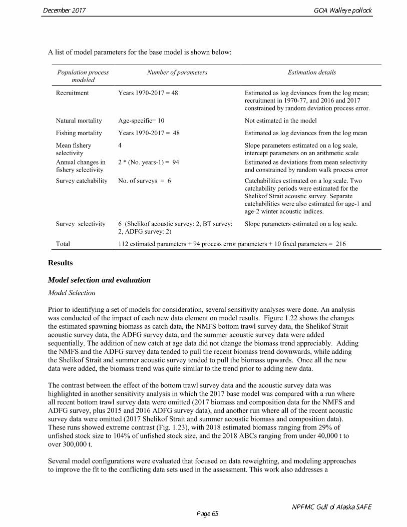
A list of model parameters for the base model is shown below:

Population process modeled

Number of parameters Estimation details

Recruitment Years 1970-2017 = 48 Estimated as log deviances from the log mean; recruitment in 1970-77, and 2016 and 2017 constrained by random deviation process error.

Natural mortality Age-specific= 10 Not estimated in the model

Fishing mortality Years 1970-2017 = 48 Estimated as log deviances from the log mean

Mean fishery selectivity

4 Slope parameters estimated on a log scale, intercept parameters on an arithmetic scale

Annual changes in fishery selectivity

2 * (No. years-1) = 94 Estimated as deviations from mean selectivity and constrained by random walk process error

Survey catchability No. of surveys = 6 Catchabilities estimated on a log scale. Two catchability periods were estimated for the Shelikof Strait acoustic survey. Separate catchabilities were also estimated for age-1 and age-2 winter acoustic indices.

Survey selectivity 6 (Shelikof acoustic survey: 2, BT survey: 2, ADFG survey: 2)

Slope parameters estimated on a log scale.

Total 112 estimated parameters + 94 process error parameters + 10 fixed parameters = 216 Results

Model selection and evaluation Model Selection Prior to identifying a set of models for consideration, several sensitivity analyses were done. An analysis was conducted of the impact of each new data element on model results. Figure 1.22 shows the changes the estimated spawning biomass as catch data, the NMFS bottom trawl survey data, the Shelikof Strait acoustic survey data, the ADFG survey data, and the summer acoustic survey data were added sequentially. The addition of new catch at age data did not change the biomass trend appreciably. Adding the NMFS and the ADFG survey data tended to pull the recent biomass trend downwards, while adding the Shelikof Strait and summer acoustic survey tended to pull the biomass upwards. Once all the new data were added, the biomass trend was quite similar to the trend prior to adding new data. The contrast between the effect of the bottom trawl survey data and the acoustic survey data was highlighted in another sensitivity analysis in which the 2017 base model was compared with a run where all recent bottom trawl survey data were omitted (2017 biomass and composition data for the NMFS and ADFG survey, plus 2015 and 2016 ADFG survey data), and another run where all of the recent acoustic survey data were omitted (2017 Shelikof Strait and summer acoustic biomass and composition data). These runs showed extreme contrast (Fig. 1.23), with 2018 estimated biomass ranging from 29% of unfished stock size to 104% of unfished stock size, and the 2018 ABCs ranging from under 40,000 t to over 300,000 t. Several model configurations were evaluated that focused on data reweighting, and modeling approaches to improve the fit to the conflicting data sets used in the assessment. This work also addresses a

recommendation during the 2016 review to explore models with time-varying catchability for the Shelikof Strait acoustic survey. Alternative models that were evaluated are listed below.

Model 16.2—last year’s base model with new data. Model 17.1—Age composition data reweighted using the Francis (2011) method. Model 17.2—Same as model 17.1, but with random walks in survey catchability for the Shelikof Strait acoustic survey and the ADFG survey. Model 17.3—Same as 17.2, but a smaller penalty on variation in catchability. Model 17.4—Same as 17.2, but with an offset for natural mortality for the 2012 year class.

Models were compared by examining model fits (Table 1.19) and plotting the estimated spawning biomass (Fig. 1.24). Since 2014, iterative reweighting has been done for composition data based on the harmonic mean of effective sample size (McAllister and Ianelli 1997). An alternative approach developed by Francis (2011) (Method TA1.8 in Appendix Table A1) accounts for positive correlations in proportions for nearby ages, which the McAllister and Ianelli method does not. We applied the Francis method starting from the original input sample sizes. Some experimentation suggested that final weights were not sensitive to different starting values. When the Francis (2011) method was applied, the revised input sample sizes were generally lower than from the McAllister and Ianelli method, as is usually the case. Revised input sample sizes were between 86% and 46% percent of those resulting from McAllister and Ianelli method. Comparison of spawning biomass trends for different reweighting procedures indicated that model results were not particularly sensitive to different approaches (Fig. 1.25). The Francis method seemed to be robust and gave reasonable results. Therefore Model 17.1, which formed the base for further model exploration, used the Francis method for reweighting. Model 17.2 and model 17.3 explored models in which survey catchability was allowed to vary from one year to the next for the Shelikof Strait acoustic survey and the ADFG bottom trawl survey. For the Shelikof Strait acoustic survey, catchability may vary because the fraction of the stock spawning in Shelikof Strait is not constant. For the ADFG survey, the fraction of the stock in the nearshore areas covered by the survey may vary from one year to the next. Interannual variation in catchability was also considered for the NMFS bottom trawl survey, but the estimated changes in catchability showed no strong patterns, so variation in catchability for this survey was not modeled. Two ways to model variation is catchability were considered, a random error process and a random walk process. Both approaches estimate catchability as a log-scale mean plus a log-scale random deviation, but for a random error process there a likelihood penalty term for the annual deviations, while for the random walk process there is a likelihood penalty term for the first difference of the deviations (See Appendix B). Both methods gave reasonable results (Fig. 1.26). The random walk approach was considered the most appropriate way to model this process, since the even the random error approach indicated there were long-term patterns in catchability. Models 17.2 and model 17.3 both used random walk error process with a penalized likelihood. The difference between the two models is that that penalty term (analogous to the standard deviation of the annual change) was 0.05 for model 17.2, and 0.10 for model 17.3. Although this is a type of random effects model, and approaches have been developed to estimate variance terms for random effects models (Thorson et al. 2015), these methods are new and still relatively untested in actual assessments. We were unable to explore these approaches in this assessment, but intend to do so in the future. Comparison of estimated catchability patterns for the Shelikof Strait acoustic survey (Fig. 1.27) indicated that both models improved the fit to the biomass estimates, but it was still not possible to fit the very high 2017 data point even when catchability pattern was allowed to be very flexible. Similar results were obtained for the ADFG bottom trawl survey (Fig. 1.28). We preferred model 17.2 over model 17.3 because we had

concerns that model 17.3 may be overfitting the survey biomass estimates, and because catchability for model 17.2 in 2017 was 0.83, which is similar to the ratio of biomass in Shelikof Strait to the total surveyed biomass in winter of 2017 (85%), when comprehensive survey of known pollock spawning locations in the GOA was conducted. A final model evaluation considered whether the unusual 2017 survey results could be accounted for by changes in the natural mortality of the 2012 year class, which is almost certainly the largest year class to recruit to the GOA pollock stock in more than 30 years. Some authors (Axelson et al. 2001, Engelhard and Heino 2006) have hypothesized that a strong year class can overwhelm its predators, producing a dilution effect that results in the year class experiencing reduced natural mortality. This was explored in model 17.4 by estimating a multiplicative term on natural mortality that applied only the 2012 year class from age 1 in 2013 to age 5 in 2017. The estimated multiplier was 0.74, indicating that natural mortality was 26% lower for this year class. Examination of the results for this model indicate that recruitment strength for the 2012 year class was estimated at 12.3 billion rather than 24.1 billion for model 17.2, suggesting that there may be a tradeoff between estimate of year class strength and cohort-specific natural mortality. The change in log likelihood between model 17.4 and 17.2 was only 1.5, suggesting that this was probably not a significant improvement in the model. Therefore model 17.4 was not considered further. On the basis of the above considerations, model 17.2 was selected as the base model, and a final turning step was done using the Francis (2011) approach. The age-1 and the age-2 Shelikof acoustic indices were also iteratively reweighted using RMSE as a tuning variable. All composition data components were reweighted slightly, but model results were nearly unchanged. Model Evaluation The fit of model 17.2 to age composition data was evaluated using plots of observed and predicted age composition and residual plots. Plots show the fit to fishery age composition (Fig. 1.29, Fig. 1.30), Shelikof Strait acoustic survey age composition (Fig. 1.31, Fig. 1.32), NMFS trawl survey age composition (Fig. 1.33, Fig. 1.34), and ADFG trawl survey age composition (Fig. 1.34, Fig. 1.35). Model fits to fishery age composition data are adequate in most years. The largest residuals tended to be at ages 1-2 in the NMFS bottom trawl survey due to inconsistencies between the initial estimates of abundance and subsequent information about year class size. Model fits to biomass estimates follow general trends in survey time series are fit reasonably well (Fig. 1.36 and Fig. 1.37), although large residuals are evident in 2017 for the Shelikof Strait acoustic survey and the NMFS bottom trawl survey. In addition, the model is unable to fit the extremely low values for the ADFG survey in 2015-2017, though otherwise the fit to this survey is quite good. The fit to the age-1 and age-2 acoustic indices appeared adequate though variable (Fig. 1.38). Time series results Parameter estimates and model output are presented in a series of tables and figures. Estimated survey and fishery selectivity for different periods are given in Table 1.20 (see also Fig. 1.39). Table 1.21 gives the estimated population numbers at age for the years 1970-2017. Table 1.22 gives the estimated time series of age 3+ population biomass, age-1 recruitment, and harvest rate (catch/3+ biomass) for 1977-2017 (see also Fig. 1.40). Table 1.23 gives coefficients of variation and 95% confidence intervals for age-1 recruitment and spawning stock biomass. Stock size peaked in the early 1980s at approximately 80% of the proxy for unfished stock size (B100% = mean 1978-2016 recruitment multiplied by the spawning biomass per recruit in the absence of fishing (SPR@F=0)). In 1999, the stock dropped below the B40% for the first time since the early 1980s, reached a minimum in 2003 of 26% of unfished stock size. Over the years 2009-2013 stock size has shown a strong upward trend from 36% to 65% of unfished

stock size, but declined to 39% of unfished stock size in 2016. The spawning stock is projected to increase again in 2018 as the strong 2012 year class continues to mature to the spawning population. Figure 1.41 shows the historical pattern of exploitation of the stock both as a time series of SPR and fishing mortality compared to the current estimates of biomass and fishing mortality reference points. Except from the mid-1970s to mid-1980s fishing mortalities has generally been lower than the current OFL definition, and in nearly all years was lower than the FMSY proxy of F35% . Retrospective comparison of assessment results A retrospective comparison of assessment results for the years 1993-2017 indicates the current estimated trend in spawning biomass for 1990-2017 is consistent with previous estimates (Fig. 1.42). All time series show a similar pattern of decreasing spawning biomass in the 1990s, a period of greater stability in 2000s, followed by an increase starting in 2008. A moderate retrospective pattern is evident for recent assessments, where the spawning biomass was revised upwards with each assessment. The estimated 2017 age composition from the current assessment is reasonably consistent with the projected 2017 age composition from the 2016 assessment (Fig. 1.42). The largest change is the estimate of the age-1 fish (2016 year class), which is much lower based on this year’s survey results indicating weak age-1 recruitment instead of average recruitment as was assumed in last year’s assessment. Retrospective analysis of base model A retrospective analysis consists of dropping the data year-by-year from the current model, and provides an evaluation of the stability of the current model as new data are added. Figure 1.43 shows a retrospective plot with data sequentially removed back to 2007. There is up to 23% error in the assessment (if the current assessment is accepted as truth), but usually the errors are much smaller. There is relatively modest positive retrospective pattern to errors in the assessment, and the revised Mohn’s ρ (Mohn 1999) for ending year spawning biomass is 0.066, which does not indicate a concern with retrospective bias. Stock productivity Recruitment of GOA pollock is more variable (CV = 0.99) than Eastern Bering Sea pollock (CV = 0.59). Other North Pacific groundfish stocks, such as sablefish and Pacific ocean perch, also have high recruitment variability. However, unlike sablefish and Pacific ocean perch, pollock have a short generation time (~8 years), so that large year classes do not persist in the population long enough to have a buffering effect on population variability. Because of these intrinsic population characteristics, the typical pattern of biomass variability for GOA pollock will be sharp increases due to strong recruitment, followed by periods of gradual decline until the next strong year class recruits to the population. GOA pollock is more likely to show this pattern than other groundfish stocks in the North Pacific due to the combination of a short generation time and high recruitment variability. Since 1980, strong year classes have occurred every four to six years, although this pattern appears much weaker since 2004 (Fig. 1.40). The 2012 year class still appears to be very strong in based on the current assessment, and appears to be strongest year class since the 1970s. Because of high recruitment variability, the mean relationship between spawning biomass and recruitment is difficult to estimate despite good contrast in spawning biomass. Strong and weak year classes have been produced at high and low level of spawning biomass. Spawner productivity is higher on average at low spawning biomass compared to high spawning biomass, indicating that survival of eggs to recruitment is density-dependent (Fig. 1.44). However, this pattern of density-dependent survival only emerges on a decadal scale, and could be confounded with environmental variability on the same temporal scale. These decadal trends in spawner productivity have produced the pattern of increase and decline in the GOA pollock population.

The last two decades have been a period of relatively low spawner productivity. In the last couple of year spawner productivity has dropped very steeply. Age-1 recruitment in 2016 is estimated to be the lowest in the time series, and age-1 recruitment in 2017 is estimated to 20% of the long-term average, though these estimates remain very uncertain. Harvest Recommendations

Reference fishing mortality rates and spawning biomass levels Since 1997, GOA pollock have been managed under Tier 3 of the NPFMC tier system. In Tier 3, reference mortality rates are based on the spawning biomass per recruit (SPR), while biomass reference levels are estimated by multiplying the SPR by average recruitment. Estimates of the FSPR harvest rates were obtained using the life history characteristics of GOA pollock (Table 1.24). Spawning biomass reference levels were based on mean 1978-2015 age-1 recruitment (5.595 billion), which is similar to the mean value in last year’s assessment. Spawning was assumed to occur on March 15th, and female spawning biomass was calculated using mean weight at age for the Shelikof Strait acoustic surveys in 2013-2017 to estimate current reproductive potential. A substantial long-term increase in pollock weight-at-age has been observed, though recently the trend in weight-at-age has reversed, begun to decline steeply (Fig. 1.20). The factors which caused this pattern are unclear, but are likely to involve both density-dependent factors and environmental forcing. The SPR at F=0 was estimated as 0.107 kg/recruit at age one. FSPR rates depend on the selectivity pattern of the fishery. Selectivity has changed as the fishery evolved from a foreign fishery occurring along the shelf break to a domestic fishery on spawning aggregations and in nearshore waters (Fig. 1.1). For SPR calculations, selectivity was based on the average for 2012-2016 to reflect current selectivity patterns. GOA pollock FSPR harvest rates are given below:

FSPR rate Fishing mortality Equilibrium under average 1978-2016 recruitment

Avg. Recr. (Million)

Total 3+ biom. (1000 t)

Female spawning biom. (1000 t)

Catch (1000 t)

Harvest rate

100.0% 0.000 5595 2203 596 0 0.0% 40.0% 0.255 5595 1270 238 176 13.8% 35.0% 0.302 5595 1186 209 191 16.1%

The B40% estimate of 238,000 t represents an 11% decrease from the B40% estimate of 267,000 t in the 2015 assessment, which is due to the continuing decline in spawning weight at age and mean recruitment. The base model projection of female spawning biomass in 2018 is 342,683 t, which is 57.5% of unfished spawning biomass (based on average post-1977 recruitment) and above B40% (238,000 t), thereby placing GOA pollock in sub-tier “a” of Tier 3. 2018 acceptable biological catch The definitions of OFL and maximum permissible FABC under Amendment 56 provide a buffer between the overfishing level and the intended harvest rate, as required by NMFS national standard guidelines. Since estimates of stock biomass from assessment models are uncertain, the buffer between OFL and ABC provides a margin of safety so that assessment error will not result in the OFL being inadvertently exceeded. For GOA pollock, the maximum permissible FABC harvest rate is 84.6% of the OFL harvest rate. In 2001 assessment, a more conservative alternative was adopted that maintains a constant buffer between ABC and FABC at all stock levels (Table 1.25).

This alternative is given by the following

Define FF B = B

40%

35%40%

*

Stock status: 1 > B / B * , then F = F 40% Stock status: 1 B / B < 0.05 * ≤ , then )()( 0.05 - 1 / 0.05 - BB/ xF = F *

40% Stock status: 0.05 B / B * ≤ , then 0 = F This alternative has the same functional form as the maximum permissible FABC; the only difference is that it declines linearly from B* (= B47%) to 0.05B* (Fig. 1.41). Projections for 2018 for FOFL, the maximum permissible FABC, and an adjusted F40% harvest rate are given in Table 1.26. ABC recommendation The recommended ABC was based on a model projection using the base model and the adjusted F40% harvest rate described above. Because the stock is above the inflection point in the harvest control rule, this alternative gives the same ABC as the maximum permissible FABC. The author’s recommended 2018 ABC is therefore 161,492 t, which is a decrease of 21% from the 2017 ABC. The recommended 2018 ABC is nearly the same as the projected 2018 ABC in the 2016 assessment (3% higher). This consistency is surprising given the strong and contrasting signals from recent survey data. In 2019, the ABC based an adjusted F40% harvest rate is 106,568 t. The OFL in 2017 is 187,059 t, and the OFL in 2019 if the recommended ABC is taken in 2017 is 131,170 t. It should be noted that there is likely to be a continuing decline in the ABC over the next few years, particularly if low recruitment continues. ABCs as low as 70,000 t may occur by 2020. The new survey data for 2017 included the Shelikof Strait acoustic survey, the NMFS bottom trawl, summer acoustic survey, and the ADFG bottom trawl survey. Survey data in 2017 are highly contrasting, with both acoustic surveys indicating large or increasing biomass, and both bottom trawl surveys indicating a steep decline in recent years. These divergent trends are likely due to changes in the availability of pollock to different surveying methods, though research is need to confirm this hypothesis. Other characteristics of the GOA pollock stock are showed unusual patterns, including changes in growth and maturation, very low recruitment, and unequal sex ratios. These unusual patterns suggest we are entering a period of greater uncertainty concerning pollock status. To evaluate the probability that the stock will drop below the B20% threshold, we projected the stock forward for five years using the author’s recommended fishing mortality schedule. This projection incorporates uncertainty in stock status, uncertainty in the estimate of B20%, and variability in future recruitment. We then sampled from the likelihood of future spawning biomass using Markov chain Monte Carlo (MCMC). A chain of 1,000,000 samples was thinned by selecting every 200th sample. Analysis of the thinned MCMC chain indicates that probability of the stock dropping below B20% will be close to zero until 2022, when the probability is estimated to be 0.0082 (Fig. 1.45).

Projections and Status Determination A standard set of projections is required for stocks managed under Tier 3 of Amendment 56. This set of projections encompasses seven harvest scenarios designed to satisfy the requirements of Amendment 56, the National Environmental Protection Act, and the Magnuson-Stevens Fishery Conservation and Management Act (MSFCMA). For each scenario, the projections begin with the 2017 numbers at age at the start of the year as estimated by the assessment model, and assume the 2017 catch will be equal to 172,500 t (84.7% of the ABC, the estimated catch as of Oct 1, plus all of the D season quota). In each year, the fishing mortality rate is determined by the spawning biomass in that year and the respective harvest scenario. Recruitment is drawn from an inverse Gaussian distribution whose parameters consist of maximum likelihood estimates determined from recruitments during 1978-2016 as estimated by the assessment model. Spawning biomass is computed in each year based on the time of peak spawning (March 15) using the maturity and weight schedules in Table 1.24. This projection scheme is run 1000 times to obtain distributions of possible future stock sizes, fishing mortality rates, and catches. Five of the seven standard scenarios are used in an Environmental Assessment prepared in conjunction with the final SAFE. These five scenarios, which are designed to provide a range of harvest alternatives that are likely to bracket the final TAC for 2018, are as follows (“max FABC” refers to the maximum permissible value of FABC under Amendment 56):

Scenario 1: In all future years, F is set equal to max FABC. (Rationale: Historically, TAC has been constrained by ABC, so this scenario provides a likely upper limit on future TACs.)

Scenario 2: In all future years, F is set equal to the FABC recommended in the assessment.

Scenario 3: In all future years, F is set equal to the five-year average F (2013-2017). (Rationale: For some stocks, TAC can be well below ABC, and recent average F may provide a better indicator of FTAC than FABC.)

Scenario 4: In all future years, F is set equal to F75%. (Rationale: This scenario represents a very conservative harvest rate and was requested by the Regional Office based on public comment.)

Scenario 5: In all future years, F is set equal to zero. (Rationale: In extreme cases, TAC may be set at a level close to zero.)

Two other scenarios are needed to satisfy the MSFCMA’s requirement to determine whether a stock is currently in an overfished condition or is approaching an overfished condition. These two scenarios are as follows (for Tier 3 stocks, the MSY level is defined as B35%):

Scenario 6: In all future years, F is set equal to FOFL. (Rationale: This scenario determines whether a stock is overfished. If the stock is expected to be 1) above its MSY level in 2017 or 2) above 1/2 of its MSY level in 2017 and above its MSY level in 2027 under this scenario, then the stock is not overfished)

Scenario 7: In 2018 and 2019, F is set equal to max FABC, and in all subsequent years, F is set equal to FOFL. (Rationale: This scenario determines whether a stock is approaching an overfished condition. If the stock is expected to be 1) above its MSY level in 2019, or 2) above 1/2 of its MSY level in 2019 and above its MSY level in 2029 under this scenario, then the stock is not approaching an overfished condition.)

Results from scenarios 1-5 are presented in Table 1.26. Mean spawning biomass is projected to peak in

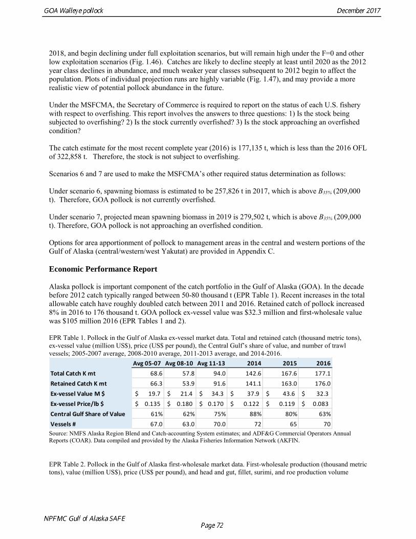
2018, and begin declining under full exploitation scenarios, but will remain high under the F=0 and other low exploitation scenarios (Fig. 1.46). Catches are likely to decline steeply at least until 2020 as the 2012 year class declines in abundance, and much weaker year classes subsequent to 2012 begin to affect the population. Plots of individual projection runs are highly variable (Fig. 1.47), and may provide a more realistic view of potential pollock abundance in the future. Under the MSFCMA, the Secretary of Commerce is required to report on the status of each U.S. fishery with respect to overfishing. This report involves the answers to three questions: 1) Is the stock being subjected to overfishing? 2) Is the stock currently overfished? 3) Is the stock approaching an overfished condition? The catch estimate for the most recent complete year (2016) is 177,135 t, which is less than the 2016 OFL of 322,858 t. Therefore, the stock is not subject to overfishing. Scenarios 6 and 7 are used to make the MSFCMA’s other required status determination as follows: Under scenario 6, spawning biomass is estimated to be 257,826 t in 2017, which is above B35% (209,000 t). Therefore, GOA pollock is not currently overfished. Under scenario 7, projected mean spawning biomass in 2019 is 279,502 t, which is above B35% (209,000 t). Therefore, GOA pollock is not approaching an overfished condition. Options for area apportionment of pollock to management areas in the central and western portions of the Gulf of Alaska (central/western/west Yakutat) are provided in Appendix C. Economic Performance Report Alaska pollock is important component of the catch portfolio in the Gulf of Alaska (GOA). In the decade before 2012 catch typically ranged between 50-80 thousand t (EPR Table 1). Recent increases in the total allowable catch have roughly doubled catch between 2011 and 2016. Retained catch of pollock increased 8% in 2016 to 176 thousand t. GOA pollock ex-vessel value was $32.3 million and first-wholesale value was $105 million 2016 (EPR Tables 1 and 2). EPR Table 1. Pollock in the Gulf of Alaska ex-vessel market data. Total and retained catch (thousand metric tons), ex-vessel value (million US$), price (US$ per pound), the Central Gulf’s share of value, and number of trawl vessels; 2005-2007 average, 2008-2010 average, 2011-2013 average, and 2014-2016.

Source: NMFS Alaska Region Blend and Catch-accounting System estimates; and ADF&G Commercial Operators Annual Reports (COAR). Data compiled and provided by the Alaska Fisheries Information Network (AKFIN. EPR Table 2. Pollock in the Gulf of Alaska first-wholesale market data. First-wholesale production (thousand metric tons), value (million US$), price (US$ per pound), and head and gut, fillet, surimi, and roe production volume

Avg 05-07 Avg 08-10 Avg 11-13 2014 2015 2016Total Catch K mt 68.6 57.8 94.0 142.6 167.6 177.1Retained Catch K mt 66.3 53.9 91.6 141.1 163.0 176.0Ex-vessel Value M $ 19.7$ 21.4$ 34.3$ 37.9$ 43.6$ 32.3$ Ex-vessel Price/lb $ 0.135$ 0.180$ 0.170$ 0.122$ 0.119$ 0.083$ Central Gulf Share of Value 61% 62% 75% 88% 80% 63%Vessels # 67.0 63.0 70.0 72 65 70

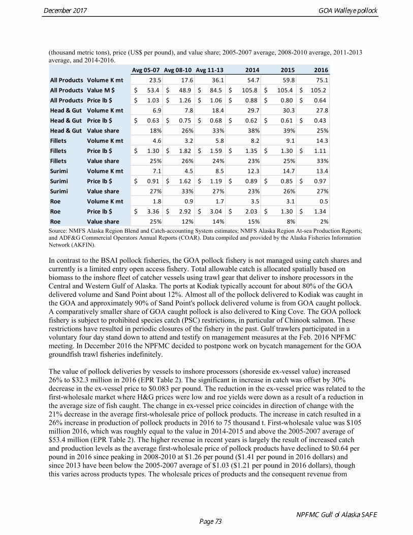
(thousand metric tons), price (US$ per pound), and value share; 2005-2007 average, 2008-2010 average, 2011-2013 average, and 2014-2016.

Source: NMFS Alaska Region Blend and Catch-accounting System estimates; NMFS Alaska Region At-sea Production Reports; and ADF&G Commercial Operators Annual Reports (COAR). Data compiled and provided by the Alaska Fisheries Information Network (AKFIN). In contrast to the BSAI pollock fisheries, the GOA pollock fishery is not managed using catch shares and currently is a limited entry open access fishery. Total allowable catch is allocated spatially based on biomass to the inshore fleet of catcher vessels using trawl gear that deliver to inshore processors in the Central and Western Gulf of Alaska. The ports at Kodiak typically account for about 80% of the GOA delivered volume and Sand Point about 12%. Almost all of the pollock delivered to Kodiak was caught in the GOA and approximately 90% of Sand Point's pollock delivered volume is from GOA caught pollock. A comparatively smaller share of GOA caught pollock is also delivered to King Cove. The GOA pollock fishery is subject to prohibited species catch (PSC) restrictions, in particular of Chinook salmon. These restrictions have resulted in periodic closures of the fishery in the past. Gulf trawlers participated in a voluntary four day stand down to attend and testify on management measures at the Feb. 2016 NPFMC meeting. In December 2016 the NPFMC decided to postpone work on bycatch management for the GOA groundfish trawl fisheries indefinitely. The value of pollock deliveries by vessels to inshore processors (shoreside ex-vessel value) increased 26% to $32.3 million in 2016 (EPR Table 2). The significant in increase in catch was offset by 30% decrease in the ex-vessel price to $0.083 per pound. The reduction in the ex-vessel price was related to the first-wholesale market where H&G prices were low and roe yields were down as a result of a reduction in the average size of fish caught. The change in ex-vessel price coincides in direction of change with the 21% decrease in the average first-wholesale price of pollock products. The increase in catch resulted in a 26% increase in production of pollock products in 2016 to 75 thousand t. First-wholesale value was $105 million 2016, which was roughly equal to the value in 2014-2015 and above the 2005-2007 average of $53.4 million (EPR Table 2). The higher revenue in recent years is largely the result of increased catch and production levels as the average first-wholesale price of pollock products have declined to $0.64 per pound in 2016 since peaking in 2008-2010 at $1.26 per pound ($1.41 per pound in 2016 dollars) and since 2013 have been below the 2005-2007 average of $1.03 ($1.21 per pound in 2016 dollars), though this varies across products types. The wholesale prices of products and the consequent revenue from

Avg 05-07 Avg 08-10 Avg 11-13 2014 2015 2016All Products Volume K mt 23.5 17.6 36.1 54.7 59.8 75.1All Products Value M $ 53.4$ 48.9$ 84.5$ 105.8$ 105.4$ 105.2$ All Products Price lb $ 1.03$ 1.26$ 1.06$ 0.88$ 0.80$ 0.64$ Head & Gut Volume K mt 6.9 7.8 18.4 29.7 30.3 27.8Head & Gut Price lb $ 0.63$ 0.75$ 0.68$ 0.62$ 0.61$ 0.43$ Head & Gut Value share 18% 26% 33% 38% 39% 25%Fillets Volume K mt 4.6 3.2 5.8 8.2 9.1 14.3Fillets Price lb $ 1.30$ 1.82$ 1.59$ 1.35$ 1.30$ 1.11$ Fillets Value share 25% 26% 24% 23% 25% 33%Surimi Volume K mt 7.1 4.5 8.5 12.3 14.7 13.4Surimi Price lb $ 0.91$ 1.62$ 1.19$ 0.89$ 0.85$ 0.97$ Surimi Value share 27% 33% 27% 23% 26% 27%Roe Volume K mt 1.8 0.9 1.7 3.5 3.1 0.5Roe Price lb $ 3.36$ 2.92$ 3.04$ 2.03$ 1.30$ 1.34$ Roe Value share 25% 12% 14% 15% 8% 2%

production must be viewed from within the context of the broader market for pollock which is largely driven by activity in the BSAI and globally. Since 2005 the volume of catch in the GOA has been roughly 5%-10% the size of the catch volume in the BSAI and approximately 3% of the global pollock catch. Fluctuations in GOA catch and production volumes have at most only a marginal impact on global pollock markets. Furthermore, one of the main product produced for GOA pollock is head-and-gut (H&G), a low price product type which is produced in high quantities by Russia. While the GOA pollock fishery experienced low catch years in 2007-2009, that approximately coincided with the lows in the BSAI from 2008-2010, it was the low catch volumes in the BSAI and other global market events which ultimately drove price changes and will be explored in more detail below. EPR Tables 1-3 display three distinguishable periods in pollock markets. From 2001-2008 pollock catches in Alaska were high at approximately 1.5 million t. The U.S. (Alaska) accounted for over 50% of the global pollock catch (EPR Table 3). Between 2008-2010 conservation reductions in the pollock total allowable catch (TAC) trimmed catches in Alaska to an average 930 thousand t. The supply reduction resulted in price increases for most pollock products, which mitigated the short-term revenue loss (EPR Table 2). Over this same period, the pollock catch in Russia increased from an average of 1 million t in 2005-2007 to 1.4 million t in 2008-2010 and Russia’s share of global catch increased to over 50% and the U.S. share decreased to 35%. Russia lacks the primary processing capacity of the U.S. and much of their catch is exported to China and is re-processed as twice-frozen fillets. Around the mid- to late-2000s, buyers in Europe, an important segment of the fillet market, started to source fish products with the MSC sustainability certification, and some major retailers in the U.S. later began to follow suit. Asian markets, an important export destination for a number of pollock products, have shown less interest in requiring MSC certification. The U.S. was the only producer of MSC certified pollock until 2013 when roughly 50% of the Russian catch became MSC certified. Since 2010 the U.S. pollock stock rebounded with catches in the BSAI ranging from 1.3-1.5 million t and Russia’s catch has stabilized at 1.5 to 1.6 million t. The majority of pollock is exported; consequently exchange rates can have a significant impact on market dynamics, particularly the Dollar-Yen and Dollar-Euro. Additionally, pollock more broadly competes with other whitefish that, to varying degrees, can serve as substitutes depending on the product. GOA pollock fisheries became certified by the Marine Stewardship Council (MSC) in 2005, a NGO based third-party sustainability certification, which some buyers seek. In 2015 the official U.S. market name changed from “Alaska pollock” to “pollock” enabling U.S. retailers to differentiate between pollock caught in Alaska and Russia.

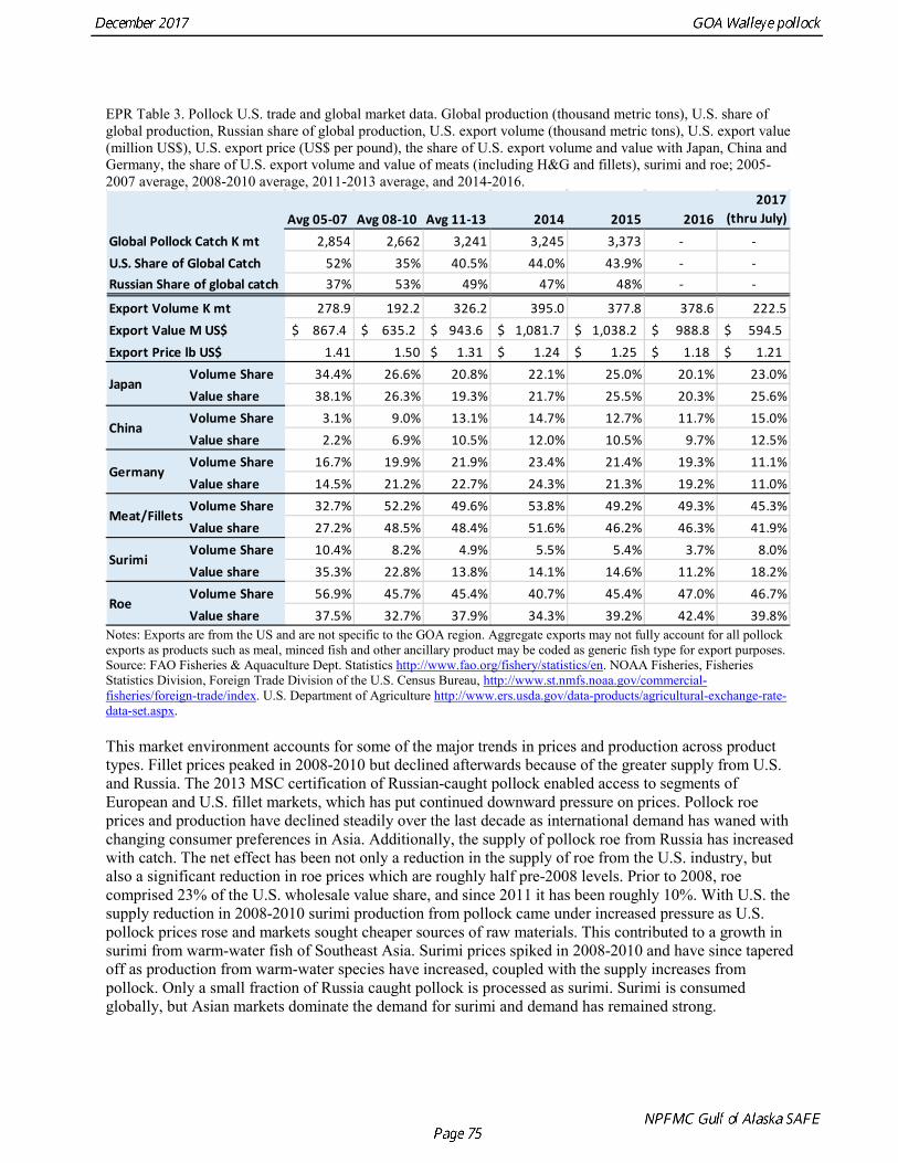
EPR Table 3. Pollock U.S. trade and global market data. Global production (thousand metric tons), U.S. share of global production, Russian share of global production, U.S. export volume (thousand metric tons), U.S. export value (million US$), U.S. export price (US$ per pound), the share of U.S. export volume and value with Japan, China and Germany, the share of U.S. export volume and value of meats (including H&G and fillets), surimi and roe; 2005-2007 average, 2008-2010 average, 2011-2013 average, and 2014-2016.

Notes: Exports are from the US and are not specific to the GOA region. Aggregate exports may not fully account for all pollock exports as products such as meal, minced fish and other ancillary product may be coded as generic fish type for export purposes. Source: FAO Fisheries & Aquaculture Dept. Statistics http://www.fao.org/fishery/statistics/en. NOAA Fisheries, Fisheries Statistics Division, Foreign Trade Division of the U.S. Census Bureau, http://www.st.nmfs.noaa.gov/commercial-fisheries/foreign-trade/index. U.S. Department of Agriculture http://www.ers.usda.gov/data-products/agricultural-exchange-rate-data-set.aspx. This market environment accounts for some of the major trends in prices and production across product types. Fillet prices peaked in 2008-2010 but declined afterwards because of the greater supply from U.S. and Russia. The 2013 MSC certification of Russian-caught pollock enabled access to segments of European and U.S. fillet markets, which has put continued downward pressure on prices. Pollock roe prices and production have declined steadily over the last decade as international demand has waned with changing consumer preferences in Asia. Additionally, the supply of pollock roe from Russia has increased with catch. The net effect has been not only a reduction in the supply of roe from the U.S. industry, but also a significant reduction in roe prices which are roughly half pre-2008 levels. Prior to 2008, roe comprised 23% of the U.S. wholesale value share, and since 2011 it has been roughly 10%. With U.S. the supply reduction in 2008-2010 surimi production from pollock came under increased pressure as U.S. pollock prices rose and markets sought cheaper sources of raw materials. This contributed to a growth in surimi from warm-water fish of Southeast Asia. Surimi prices spiked in 2008-2010 and have since tapered off as production from warm-water species have increased, coupled with the supply increases from pollock. Only a small fraction of Russia caught pollock is processed as surimi. Surimi is consumed globally, but Asian markets dominate the demand for surimi and demand has remained strong.

Avg 05-07 Avg 08-10 Avg 11-13 2014 2015 20162017

(thru July)

2,854 2,662 3,241 3,245 3,373 - -52% 35% 40.5% 44.0% 43.9% - -37% 53% 49% 47% 48% - -

278.9 192.2 326.2 395.0 377.8 378.6 222.5867.4$ 635.2$ 943.6$ 1,081.7$ 1,038.2$ 988.8$ 594.5$

1.41 1.50 1.31$ 1.24$ 1.25$ 1.18$ 1.21$ Volume Share 34.4% 26.6% 20.8% 22.1% 25.0% 20.1% 23.0%Value share 38.1% 26.3% 19.3% 21.7% 25.5% 20.3% 25.6%Volume Share 3.1% 9.0% 13.1% 14.7% 12.7% 11.7% 15.0%Value share 2.2% 6.9% 10.5% 12.0% 10.5% 9.7% 12.5%Volume Share 16.7% 19.9% 21.9% 23.4% 21.4% 19.3% 11.1%Value share 14.5% 21.2% 22.7% 24.3% 21.3% 19.2% 11.0%Volume Share 32.7% 52.2% 49.6% 53.8% 49.2% 49.3% 45.3%Value share 27.2% 48.5% 48.4% 51.6% 46.2% 46.3% 41.9%Volume Share 10.4% 8.2% 4.9% 5.5% 5.4% 3.7% 8.0%Value share 35.3% 22.8% 13.8% 14.1% 14.6% 11.2% 18.2%Volume Share 56.9% 45.7% 45.4% 40.7% 45.4% 47.0% 46.7%Value share 37.5% 32.7% 37.9% 34.3% 39.2% 42.4% 39.8%

Germany

Meat/Fillets

Surimi

Roe

Global Pollock Catch K mtU.S. Share of Global CatchRussian Share of global catch

Export Volume K mtExport Value M US$Export Price lb US$

Japan

China

The portfolios of products produced in the GOA differs somewhat from the BSAI. The primary products processed from pollock in the BSAI are fillets, surimi and roe, with each accounting for approximately 40%, 35%, and 10% of first-wholesale value. In the GOA the primary products are head-and-gut, surimi, fillets, and roe, each have typically accounted for approximately 35%, 25%, 25%, and 13% of first-wholesale value in recent years. In terms of GOA production, head-and-gut, surimi, and fillets each have typically accounted for approximately 50%, 25%, and 15% of production in recent years. The production shares have changed since 2005-2007, particularly for H&G. When surimi production decreased with average catch volumes in 2008-2010, but H&G production increased. In 2011-2015 proportionally more of the increases from catch have gone towards H&G production, though surimi and fillet production has increased as well at a slower rate. In 2016 low prices for H&G pollock resulted decreases in H&G’s relative share of value and volume to 25% and 37%, respectively. Fillet’s share of value and volume increased to 19% and 33%, respectively. Additionally, a reduction in the average size of fish resulted in low roe yields which reduced production and roe’s share of value to 2%. Prices for pollock products in the GOA, a shoreside fishery, are close to the prices for the corresponding products produces by the BSAI shoreside sector. The price of fillet produced in the GOA are on average about 5% higher than those on produced in the BSAI shoreside. Though in 2016 the BSAI price was higher than in the GOA. The price of roe is on average about 10% lower in the GOA than the BSAI shoreside sector. The price of products produced at-sea in the BSAI tend to be higher than comparable products produced shoreside because of the shorter time span between catch, processing and freezing. Low prices for H&G pollock and the smaller average size of fish caught were the major impediments to revenue generation in 2016. H&G pollock is largely exported to China for secondary processing and media reports indicate that the price for H&G pollock was low citing and insolvency of a major international pollock trader, significant inventories and smaller fish as contributing factors. Additionally, much of the Russian catch also goes to China as H&G for secondary processing and the weak value of the Russian Ruble could have been a contributing factor. The low price for H&G may have contributed to the increased production of fillets where prices were comparatively better. Total fillet production increased 57% to 14.3 thousand t in 2016. The average price of fillet products in the GOA decreased 14% to $1.11 per pound and is below the inflation adjusted average price of fillets in 2005-2007 of $1.53 per pound. The majority of fillet produced in the GOA are pin-bone-out (PBO). Approximately 30% of the fillets produced in Alaska are estimated to remain in the domestic market, which accounts for roughly 45% of domestic pollock fillet consumption. As recent fillet markets have become increasingly tight, the industry has tried to maintain value by increasing domestic marketing for fillet based product and creating product types that are better suited to the American palette, in addition to increased utilization of by-products. Surimi production decreased 8% to 13.4 thousand t in 2016 but remains high. Surimi production peaked in 2015 and the 2016 level is the second highest. The price for surimi increased 14% to $0.97. Surimi prices decreased in the GOA from 2013 through 2015. This trend was in contrast to the price increase in the BSAI particularly for the at-sea sector. Media reports indicate that the supply of raw surimi material continues to be constrained in Japan. Demand for surimi has remained strong though the high volume of surimi production in recent years has raised concerns that prices may begin to plateau or fall. More favorable exchange rate with Japan in 2016 may have helped to shore up prices. Roe is a high priced product that is the focus of the A season catch and destined primarily for Asian markets. Compared to 2005-2007, GOA roe production in recent years had been high because of the increased catch levels. Roe production in the GOA tapered off in 2008-2010 but rebounded with catch levels up through 2015. In 2016, roe production decreased 83% to a low of 539 t. Low roe yields from the catch of smaller fish was cited as a contributing factor. Smaller fish with lower roe yields were reported as factor in the BSAI and Russian catch as well. The smaller fish also tended to yield a lower grade roe which lowers the average roe price. However, constrained roe inventories and reduced global supply in 2016 put upward pressure on roe prices. In addition, value of the Yen against the U.S. Dollar was more

favorable in 2016 than 2015. The net effect was a 3% increase in the price of roe $1.34 in 2016. The revenue from roe decreased with the reduced production to a low of $1.6 million. Ecosystem considerations

Prey of pollock An ECOPATH model was assembled to characterize food web structure in Gulf of Alaska using diet data and population estimates during 1990-93. We use ECOPATH here simply as a tool to integrate diet data and stock abundance estimates in a consistent way to evaluate ecosystem interactions. We focus primarily on first-order trophic interactions: prey of pollock and the predators of pollock. Pollock trophic interactions occur primarily in the pelagic pathway in the food web, which leads from phytoplankton through various categories of zooplankton to planktivorous fish species such as capelin and sandlance (Fig. 1.48). The primary prey of pollock are euphausiids, but pollock also consume shrimp, which are more associated with the benthic pathway, and make up approximately 18% of age 2+ pollock diet. All ages of GOA pollock are primarily zooplanktivorous during the summer growing season (>80% by weight zooplankton in diets for juveniles and adults; Fig 1.49). While there is an ontogenetic shift in diet from copepods to larger zooplankton (primarily euphausiids) and fish, cannibalism is not as prevalent in the Gulf of Alaska as in the Eastern Bering Sea, and fish consumption is low even for large pollock (Yang and Nelson 2000). There are no extended time series of zooplankton abundance for the shelf waters of the Gulf of the Alaska—though Seward Line monitoring now extends from 1998 to the present, and efforts are underway at AFSC to develop Euphausiid abundance indices from summer acoustic surveys in the Gulf of Alaska. Brodeur and Ware (1995) provide evidence that biomass of zooplankton in the center of the Alaska Gyre was twice as high in the 1980s than in the 1950s and 1960s, consistent with a shift to positive values of the PDO since 1977. The percentage of zooplankton in diets of pollock is relatively constant throughout the 1990s (Fig. 1.49). While indices of stomach fullness exist for these survey years, a more detailed bioenergetics modeling approach would be required to examine if feeding and growth conditions have changed over time, especially given the fluctuations in GOA water temperature in recent years, as water temperature has a considerable effect on digestion and other energetic rates. Predators of pollock Initial ECOPATH model results show that the top five predators on pollock >20 cm by relative importance are arrowtooth flounder, Pacific halibut, Pacific cod, Steller sea lion (SSL), and the directed pollock fishery (Fig. 1.50). For pollock less than 20cm, arrowtooth flounder represent close to 50% of total mortality. All major predators show some diet specialization, and none depend on pollock for more than 50% of their total consumption (Fig. 1.51). Pacific halibut is most dependent on pollock (48%), followed by SSL (39%), then arrowtooth flounder (24% for juvenile and adult pollock combined), and lastly Pacific cod (18%). It is important to note that although arrowtooth flounder is the largest single source of mortality for both juvenile and adult pollock (Fig 1.50), arrowtooth depend less on pollock in their diets than do other important pollock predators. Arrowtooth consume a greater number of small pollock than do Pacific cod or Pacific halibut, which consume primarily adult fish. However, by weight, larger pollock are important to all three predators (Fig. 1.52). Size composition of pollock consumed by the western stock of Steller sea lions tend towards larger fish, and are similar to the size of cod and halibut consumed (Zeppelin et al. 2004). The diet of Pacific cod and Pacific halibut are similar in that the majority of their diet besides pollock is from the benthic pathway of the food web. Alternate prey for Steller sea lions and arrowtooth flounder are similar, and come primarily from the pelagic pathway.

Predation mortality, as estimated by ECOPATH, is extremely high for GOA pollock >20cm. Estimates for the 1990-1993 time period indicate that known sources of predation sum to 90%-120% of the total production of walleye pollock calculated from 2004 stock assessment growth and mortality rates; estimates greater than 100% may indicate a declining stock (as shown by the stock assessment trend in the early 1990s; Fig 1.53, top), or the use of mortality rates which are too low. Conversely, as >20cm pollock include a substantial number of 2-year olds, it may be that mortality rate estimates for this age range is low. In either case, predation mortality for pollock in the GOA is much greater a proportion of pollock production than as estimated by the same methods for the Bering Sea, where predation mortality (primarily pollock cannibalism) was up to 50% of total production. Aside from the long-recognized decline in Steller sea lion abundance, the major predators of pollock in the Gulf of Alaska are stable to increasing, in some cases notably so since the 1980s (Fig. 1.53, top). This high level of predation is of concern in light of the declining trend of pollock with respect to predator increases. To assess this concern, it is important to determine if natural mortality may have changed over time (e.g. the shifting control hypothesis; Bailey 2000). To examine predator interactions more closely than in the initial model, diet data of major predators in trawl surveys were examined in all survey years since 1990. Trends in total consumption of walleye pollock were calculated by the following formula:

sizepredGOAsizepredsubregionsizepredsubregionsizepred RationWLFDCBnConsumptio ,,,,,,, ⋅⋅⋅= ∑ where B(pred, size, subregion) is the biomass of a predator size class in the summer groundfish surveys in a particular survey subregion; DC is the percentage by weight of pollock in that predator group as measured from stomach samples, WLF is the weight frequency of pollock in the stomachs of that predator group pooled across the GOA region, calculated from length frequencies in stomachs and length-weight relationships from the surveys. Finally, ration is an applied yearly ration for that predator group calculated by fitting weight-at-age to the generalized von Bertalanffy growth equations as described in Essington et al. (2001). Ration is assumed fixed over time for a given size class of predator. Fig. 1.53 (bottom) shows annual total estimates of consumption of pollock (all age classes) in survey years by the four major fish predators. Other predators, shown as constant, are taken from ECOPATH modeling results and displayed for comparison. Catch is shown as reported in Table 1.1. In contrast, the line in the figure shows the historical total production (tons/year) plus yearly change in biomass (positive or negative) from the stock assessment results. In a complete accounting of pollock mortality, the height of the bars should match the height of the line. As shown, estimates of consumption greatly surpass estimates of production; fishing mortality is a relatively small proportion of total consumption. Consumption rates could be overestimated because of seasonal differences in diets; while ration is seasonally adjusted, diet proportions are based on summer data. Also, better energetic estimates of consumption would improve these estimates. In terms of the stock assessment, underestimates of production could result from underestimating natural mortality, especially at ages 2-3, underestimating the rate of decline which occurred between 1990-present, or underestimates of the total biomass of pollock; this analysis should be revisited using higher mortality at younger ages as is now assumed in the stock assessment. To better judge natural mortality, consumption was calculated for two size groups of pollock, divided at 30cm fork length. This size break, which differs from the break in the ECOPATH analysis, is based on finding minima between modes of pollock in predator diets (Fig. 1.54). This break is different from the conversion matrices used in the stock assessment; perhaps due to differences in size selection between

predators and surveys. For this analysis, it is assumed that pollock<30cm are ages 0-2 while pollock ≥30cm are age 3+ fish. Consumption of age 0-2 pollock per unit predator biomass (using survey biomass) varied considerably through survey years, although within a year all predators had similar consumption levels (Fig. 1.55, top). Correlation coefficients of consumption rates were 0.98 between arrowtooth and halibut, and 0.90 for both of these species with pollock. Correlation coefficients of these three species with cod were ~0.55 for arrowtooth and halibut and ~0.20 with pollock. The majority of this predation by weight occurred on age 2 pollock. Plotted against age 2 pollock numbers calculated from the stock assessment, consumption/biomass and total consumption by predator shows a distinct pattern (Fig. 1.55, lower two graphs). In “low” recruitment years consumption is consistently low, while in high recruitment years consumption is high, but does not increase linearly, rather consumptions seems to level out at high numbers of juvenile pollock, resembling a classic “Type II” functional response. This suggests the existence bottom-up control of juvenile consumption, in which strong year classes of pollock “overwhelm” feeding rates of predators, resulting in potentially lower juvenile mortality in good recruitment years which may amplify the recruitment. However, this result should be examined iteratively within the stock assessment, as the back-calculated numbers at age 2 assume a constant natural mortality rate. Assuming a lower mortality rate due to predator satiation would lead to lower estimates of age 2 numbers, which would make the response appear more linear. Consumption of pollock ≥30cm shows a different pattern over time. A decline of consumption per unit biomass is evident for halibut and cod (Fig. 1.55 top). Arrowtooth shows an insignificant decline; it is possible that the noise in the arrowtooth trend, mirroring the consumption of <30cm fish, is due to the choice of 30cm as an age cutoff. As a function of age 3+ assessment biomass, consumption per unit biomass and total consumption remained constant as the stock declined, and then fell off rapidly at low biomass levels in recent years (Fig. 1.55, middle and bottom). Again, this result should be approached iteratively, but it suggests increasing predation mortality on age 3+ pollock during 1990-2005, possibly requiring increased foraging effort from predators. There has been a marked decline in Pacific halibut weight at age since the 1970s that Clark et al. (1999) attributed to the 1977 regime shift without being able to determine the specific biological mechanisms that produced the change. Possibilities suggested by Clark et al. (1999) include the physiological effect of an increase in temperature, intra- and interspecific competition for prey, or a change in prey quality. The two species most dependent on pollock in the early 1990s (Pacific halibut and Steller sea lion) have both shown an exceptional biological response during the post-1977 period consistent with a reduction in carrying capacity (growth for Pacific halibut, survival for Steller sea lions). In contrast, the dominant predator on pollock in the Gulf of Alaska (arrowtooth flounder) has increased steadily in abundance over the same period and shows no evidence of decline in size at age. Given that arrowtooth flounder has a range of potential prey types to select from during periods of low pollock abundance (Fig. 1.51), we do not expect that arrowtooth would decline simply due to declines in pollock. Taken together, Figs. 1.54 and 1.55 suggest that recruitment remains bottom-up controlled even under the current estimates of high predation mortality, and may lead to strong year classes. However, top-down control seems to have increased on age 3+ pollock in recent years, perhaps as predators have attempted to maintain constant pollock consumption during a period of declining abundance. It is possible that natural mortality on adult pollock will remain high in the ecosystem in spite of decreasing pollock abundance.

Ecosystem modeling To examine the relative role of pollock natural versus fishing mortality within the GOA ecosystem, a set of simulations were run using the ECOPATH model shown in Fig. 1.48. Following the method outlined in Aydin et al. (2005), 20,000 model ecosystems were drawn from distributions of input parameters; these parameter sets were subjected to a selection/rejection criteria of species persistence resulting in approximately 500 ecosystems with nondegenerate parameters. These models, which did not begin in an equilibrium state, were projected forward using ECOSIM algorithms until equilibrium conditions were reached. For each group within the model, a perturbation experiment was run in all acceptable ecosystems by reducing the species survival (increasing mortality) by 10%, or by reducing gear effort by 10%, and reporting the percent change in equilibrium of all other species or fisheries catches. The resulting changes are reported as ranges across the generated ecosystems, with 50% and 95% confidence intervals representing the distribution of percent change in equilibrium states for each perturbation. Fig. 1.56 shows the changes in other species when simulating a 10% decline in adult pollock survival (top graph), a 10% decline in juvenile pollock survival (middle graph), and a 10% decline in pollock trawl effort. Fisheries in these simulations are governed by constant fishing mortality rates rather than harvest control rules. Only the top 20 effects are shown in each graph; note the difference in scales between each graph. The model results indicate that the largest effects of declining adult pollock survival would be declines in halibut and Steller sea lion biomass. Declines in juvenile survival would have a range of effects, including halibut and Steller sea lions, but also releasing a range of competitors for zooplankton including rockfish and shrimp. The pollock trawl itself has a lesser effect throughout the ecosystem (recall that fishing mortality is small in proportion to predation mortality for pollock); the strongest modeled effects are not on competitors for prey but on incidentally caught species (Table 1.2), with the strongest effects being on sharks. The results presented above are taken from Gulfwide weighted averages of consumption; Steller sea lions and the fishing fleet are central place foragers, making foraging trips from specific locations (ports in the case of the fishing fleet, and rookeries or haulouts for Steller sea lions). Foraging bouts (or trawl sets) begin at the surface, and foragers attack their prey from the top down. For such species, directed and local changes in fishing may have a disproportionate effect compared to the results shown here. In contrast, predation by groundfish is not as constrained geographically, and captures are likely to occur when the predator swims upwards from the bottom. Changes in the vertical distribution of pollock may tend to favor one mode of foraging over another. For example, if pollock move deeper in the water column due to surface warming, foraging groundfish might obtain an advantage over surface foragers. Alternatively, pollock may respond adaptively to predation risks from groundfish or surface foragers by changing its position in the water column. Of species affecting pollock (Fig. 1.57), arrowtooth have the largest impact on adult pollock, while bottom-up processes (phytoplankton and zooplankton) have the largest impact on juvenile pollock. It is interesting to note that the link between juvenile and adult pollock is extremely uncertain (wide error bars) within these models. Finally, of the four major predators of pollock (Fig. 1.58), all are affected by bottom-up forcing; Steller sea lions, Pacific cod, and Pacific halibut are all affected by pollock perturbations, while pollock effects on arrowtooth are much more minor.

Pair-wise correlations in predator trends were examined for consistent patterns (Fig. 1.59). For each pair-wise comparison, we used the maximum number of years available. Time series for Steller sea lions and Pacific cod begin in mid 1970s, while other time series extend back to the early 1960s. We make no attempt to evaluate statistical significance (biomass trends are highly autocorrelated), and emphasize that correlation does not imply causation. If two populations are strongly correlated in time, there are many possible explanations: both populations are responding to similar forcing, one or other is causative agent, etc. Pollock abundance, fishery catches, and Steller sea lions are positively correlated (Fig. 1.59). Since the harvest policy for pollock is a modified fixed harvest rate strategy, a positive correlation between catch and abundance would be expected. The Steller sea lion trend is more strongly correlated with pollock abundance than pollock catches, but this correlation is based on data since 1976, and does not include earlier years of low pollock abundance. The only strong inverse correlation is between arrowtooth flounder and Steller sea lions. A strong positive correlation exists between Pacific cod and Pacific halibut, and, from the 1960s to the present, between Pacific halibut and arrowtooth flounder. Several patterns are apparent in abundance trends and the diet data. First, the two predators with alternate prey in the benthic pathway, Pacific cod and Pacific halibut, covary and have been relatively stable in the post-1977 period. Second, the correlation between Pacific halibut and arrowtooth flounder (with quite different diets apart from pollock) may be due to similarities in their reproductive behavior. Both spawn offshore in late winter, and conditions that enhance onshore advection, such as El Niños, may play an important role in recruitment to nursery areas for these species (Bailey and Picquelle 2002). Finally, it is apparent that the potential for competition between Steller sea lions and arrowtooth flounder is underappreciated. Arrowtooth flounder consume both the primary prey of Steller sea lions (pollock), and alternate pelagic prey also utilized by Steller sea lions (capelin, herring, sandlance, and salmon). Arrowtooth predation on pollock occurs at a smaller size than pollock targeted by Steller sea lions. The arrowtooth flounder population is nearly unexploited, is increasing in abundance, may be increasing it’s per unit consumption of pollock, and shows no evidence of density-dependent growth. And lastly, since 1976 there has been a strong inverse correlation between arrowtooth flounder and Steller sea lion abundance that is at least consistent with competition between these species. Data Gaps and Research Priorities

Based on the 2012 CIE review of the Gulf of Alaska pollock assessment, the following research priorities are identified. Additional details on recommended pollock research are included in a document provided to the GOA Plan Team in September 2013 that summarized and responded to the CIE review.

• Reduce data sets to those that are informative about current status by removing earlier and more questionable data sets, and reducing the influence of the inconsistent data earlier in the time series.

• Improve relative weightings given to different data sets. • Consider alternative modeling platforms. • Conduct research to develop informative priors on acoustic and trawl survey selectivity and

catchability, and consider different ways to model selectivity. • Evaluate alternative ways to model fishery and survey selectivity (including asymptotic

selectivity). • Explore implications of non-constant natural mortality on pollock assessment and management.

Literature Cited

Alton, M. S., M. O. Nelson, and B. A. Megrey. 1987. Changes in the abundance and distribution of walleye pollock (Theragra chalcogramma) in the western Gulf of Alaska. Fish. Res. 5: 185-197. Alverson, D. L. And M. J. Carney. 1975. A graphic review of the growth and decay of population cohorts. Cons. int. Explor. Mer, 133-143. Anderson, P. J. and J. F. Piatt 1999. Community reorganization in the Gulf of Alaska following ocean climate regime shift. Mar. Ecol. Prog. Ser. 189:117-123. Axelsen, B.E., Anker-Nilssen, T., Fossum, P., Kvamme, C., and Nottestad, L. 2001. Pretty patterns but a simple strategy: predator-prey interactions between juvenile herring and Altlantic puffins observed with multibeam sonar. Can. J. Zool. 79:1586-1596. Aydin, K., G.A. McFarlane, J.R. King, B.A. Megrey, and K.W. Myers. 2005. Linking oceanic food webs to coastal production and growth rates of Pacific salmon (Oncorhynchus spp.), using models on three scales. Deep-sea Res, II. 52: 757-780. Bailey, K.M., P.J. Stabeno, and D.A. Powers. 1997. The role of larval retention and transport features in mortality and potential gene flow of walleye pollock. J. Fish. Biol. 51(Suppl. A):135-154. Bailey, K.M., T.J. Quinn II, P. Bentzen, and W.S. Grant. 1999. Population structure and dynamics of walleye pollock, Theragra chalcogramma. Advances in Mar. Biol. 37: 179-255. Bailey, K.M. 2000. Shifting control of recruitment of walleye pollock Theragra chalcogramma after a major climatic and ecosystem change. Mar. Ecol. Prog. Ser. 198:215-224. Bailey, K. M and S. J. Picquelle. 2002. Larval distribution of offshore spawning flatfish in the Gulf of Alaska: potential transport pathways and enhanced onshore transport during ENSO events. Mar. Ecol. Prog. Ser. 236:205-217. Baranov, F.I. 1918. On the question of the biological basis of fisheries. Nauchn. Issed. Ikhtiologicheskii Inst. Izv. 1:81-128. Barbeaux, S.J., S. Gaichas, J. Ianelli, and M.W. Dorn. 2005. Evaluation of biological sampling protocols for at-sea groundfish observers in Alaska. Alaska Fishery Research Bulletin. 11:82-101. Brodeur, R. D. and Ware, D.M. 1995. Interdecadal variability in distribution and catch rates of epipelagic nekton in the Northeast Pacific Ocean. pp. 329-356 in R. J. Beamish [Ed.] Climate change and northern fish populations. Canadian Special Publication of Fisheries and Aquatic Sciences 121. National Research Council of Canada, Ottawa. Brodziak, J., J. Ianelli, K. Lorenzen, and R.D. Methot Jr. (eds). 2011. Estimating natural mortality in stock assessment applications. U.S. Dep. Commer., NOAA Tech. Memo. NMFS-F/SPO-119, 38 p. Clark, W.G. 1999. Effects of an erroneous natural mortality rate on a simple age-structured model. Can. J. Fish. Aquat. Sci. 56:1721-1731. Clark, W. G., S. R. Hare, A. M. Parma, P. J. Sullivan, and R. J. Trumble. 1999. Decadal changes in growth and recruitment of Pacific halibut (Hippoglossus stenolepis). Can. J. Fish. Aquat. Sci. 56(2): 242-252. Deriso, R.B., T.J. Quinn II, and P.R. Neal. 1985. Catch-age analysis with auxiliary information. Can. J. Fish. Aquat. Sci. 42: 815-824. De Robertis, A., Hjellvik, V., Williamson, N. J., and Wilson, C. D. 2008. Silent ships do not always encounter more fish: comparison of acoustic backscatter recorded by a noise-reduced and a conventional research vessel. – ICES Journal of Marine Science, 65: 623–635. Dorn, M. W., and R. D. Methot. 1990. Status of the coastal Pacific whiting resource in 1989 and recommendation to management in 1990. U.S. Dep. Commer., NOAA Tech. Memo. NMFS F/NWC-182, 84 p. Dorn, M.W., S. Barbeaux, B, M. Guttormsen, B. Megrey, A. Hollowed, M. Wilkins, and K. Spalinger. 2003. Assessment of the walleye pollock stock in the Gulf of Alaska. In Stock Assessment and Fishery Evaluation Report for Groundfish Resources of

the Gulf of Alaska. Prepared by the Gulf of Alaska Groundfish Plan Team, North Pacific Fishery Management Council, P.O. Box 103136, Anchorage, AK 99510. North Pacific Fisheries Management Council, Anchorage, AK. Dorn, M.W., K. Aydin, S. Barbeaux, D. Jones, K. Spalinger, and W. Palsson. 2012. Assessment of the walleye pollock stock in the Gulf of Alaska. In Stock Assessment and Fishery Evaluation Report for Groundfish Resources of the Gulf of Alaska. Prepared by the Gulf of Alaska Groundfish Plan Team, North Pacific Fishery Management Council, P.O. Box 103136, Anchorage, AK 99510. North Pacific Fisheries Management Council, Anchorage, AK. Dorn, M.W., K. Aydin, D. Jones, W. Palsson, and K. Spalinger. 2014. Assessment of the walleye pollock stock in the Gulf of Alaska. In Stock Assessment and Fishery Evaluation Report for Groundfish Resources of the Gulf of Alaska. Prepared by the Gulf of Alaska Groundfish Plan Team, North Pacific Fishery Management Council, P.O. Box 103136, Anchorage, AK 99510. North Pacific Fisheries Management Council, Anchorage, AK. Doubleday, W.G. 1976. A least-squares approach to analyzing catch at age data. Res. Bull. Int. Comm. Northw. Atl. Fish. 12:69-81. Engelhard, G.H., and M. Heino. 2006. Climate change and the condition of herring (Clupea harengus) explain long-term trends in extent of skipped reproduction. Oecologia 149:593-603. Forrester, C.R., A.J. Beardsley, and Y. Takahashi. 1978. Groundfish, shrimp, and herring fisheries in the Bering Sea and Northeast Pacific—historical catch through 1970. International North Pacific Fisheries Commission, Bulletin Number 37. 150 p. Forrester, C.R., R.G. Bakkala, K. Okada, and J.E. Smith. 1983. Groundfish, shrimp, and herring fisheries in the Bering Sea and Northeast Pacific—historical catch statistics, 1971-1976. International North Pacific Fisheries Commission, Bulletin Number 41. 108 p. Francis, R.I.C.C. 2011. Data weighting in statistical fisheries stock assessment models. Can. J. Fish. Aquat. Sci. 68:1124-1138. Fournier, D. and C. P. Archibald. 1982. A general theory for analyzing catch at age data. Can. J. Fish. Aquat. Sci. 39:1195-1207. Fournier, D.A., H.J. Skaug, J. Ancheta, J. Ianelli, A. Magnusson, M.N. Maunder, A. Nielsen, and J. Sibert. 2012. AD Model Builder: using automatic differentiation for statistical inference of highly parameterized complex nonlinear models. Optim. Methods Softw. 27:233-249. Fritz, L. W. 1993. Trawl locations of walleye pollock and Atka mackerel fisheries in the Bering Sea, Aleutian Islands, and Gulf of Alaska from 1977-92. AFSC Processed Report 93-08. NMFS, AFSC, 7600 Sand Point Way, NE, Seattle, WA 98115. 162 p. Gislason, H, N. Daan, J. C. Rice and J. G. Pope. 2010. Size, growth, temperature and the natural mortality of marine fish. Fish and Fisheries 11:149–158. Grant, W.S. and F.M. Utter. 1980. Biochemical variation in walleye pollock Theragra chalcogramma: population structure in the southeastern Bering Sea and Gulf of Alaska. Can. J. Fish. Aquat. Sci. 37:1093-1100. Greiwank, A., and G.F. Corliss (eds.) 1991. Automatic differentiation of algorithms: theory, implementation and application. Proceedings of the SIAM Workshop on the Automatic Differentiation of Algorithms, held Jan. 6-8, Breckenridge, CO. Soc. Indust. and Applied Mathematics, Philadelphia. Gunderson, D. R. and P. H. Dygert. 1988. Reproductive effort as a predictor of natural mortality rate. J. Cons. int. Mer, 44:200-209. Hilborn, R. and C.J. Walters. 1992. Quantitative fisheries stock assessment: choice, dynamics, and uncertainty. Chapman and Hall, New York, N.Y. 570 p. Hollowed, A.B. and B.A. Megrey. 1990. Walleye pollock. In Stock Assessment and Fishery Evaluation Report for the 1991 Gulf of Alaska Groundfish Fishery. Prepared by the Gulf of Alaska Groundfish Plan Team, North Pacific Fishery Management Council, P.O. Box 103136, Anchorage, AK 99510. Hollowed, A.B., E. Brown, P. Livingston, B.A. Megrey and C. Wilson. 1995. Walleye pollock. In Stock Assessment and Fishery Evaluation Report for Gulf of Alaska As Projected for 1996. Prepared by the Gulf of Alaska Groundfish Plan Team, North Pacific Fishery Management Council, P.O. Box 103136, Anchorage, AK 99510. North Pacific Fisheries Management Council, Anchorage, AK.

Hollowed, A.B., J.N. Ianelli, P. Livingston. 2000. Including predation mortality in stock assessments: a case study for Gulf of Alaska pollock. ICES J. Mar. Sci. 57:279-293. Jones, D. T., P. H. Ressler, S. C. Stienessen, A. L. McCarthy, and K. A. Simonsen. 2014. Results of the acoustic-trawl survey of walleye pollock (Gadus chalcogrammus) in the Gulf of Alaska, June-August 2013 (DY2013-07). AFSC Processed Rep. 2014-06, 95 p. Alaska Fish. Sci. Cent., NOAA, Natl. Mar. Fish. Serv., 7600 Sand Point Way NE, Seattle WA 98115. Kastelle, C. R. and D. K. Kimura. 2006. Age validation of walleye pollock (Theragra chalcogramma) from the Gulf of Alaska using the disequilibrium of Pb-210 and Ra-226. ICES Journal of Marine Science 63:1520-1529. Kendall, A.W. Jr. and S.J. Picquelle. 1990. Egg and larval distributions of walleye pollock Theragra chalcogramma in Shelikof Strait, Gulf of Alaska. Fish. Bull., U.S. 88:133-154. Kimura, D.K. 1989. Variability, tuning, and simulation for the Doubleday-Deriso catch-at-age model. Can. J. Fish. Aquat. Sci. 46:941-949. Kimura, D.K. 1990. Approaches to age-structured separable sequential population analysis. Can. J. Fish. Aquat. Sci. 47:2364-2374. Kimura, D.K. 1991. Improved methods for separable sequential population analysis. Unpublished. Alaska Fisheries Science Center, 7600 Sand Point Way NE, Seattle, Washington 98115. Kimura, D. K. and S. Chikuni. 1989. Variability in estimating catch-in-numbers-at-age and its impact on cohort analysis. In R.J. Beamish and G.A. McFarlane (eds.), Effects of ocean variability on recruitment and an evaluation of parameters used in stock assessment models. Can. Spec. Publ. Fish. Aquat. Sci. 108:57-66. Kotwicki, S. P.H. Ressler, J.N. Ianelli, A.E. Punt and J.K. Horne. 2017. Combining data from bottom-trawl and acoustic-trawl surveys to estimate and index of abundance for semipelagic species. Can. J. Fish. Aquat. Sci. 00: 1–12 (0000) dx.doi.org/10.1139/cjfas-2016-0362 Lorenzen, K. 1996. The relationship between body weight and natural mortality in juvenile and adult fish: a comparison of natural ecosystems and aquaculture. Journal of Fish Biology 49:627-647. McAllister, M.K., and J.N. Ianelli. 1997. Bayesian stock assessment using catch-age data and the sampling-importance algorithm. Can. J. Fish. Aquat. Sci. 54(2): 284-300. McCarthy, A., S. Stienessen, M. Levine. In Press. Results of the acoustic-trawl surveys of walleye pollock (Gadus chalcogrammus) in the Gulf of Alaska, February-March 2017 (DY2017-01, DY2017-02, and DY2017-03). AFSC Processed Rep. 2017-XX, XX p. Alaska Fish. Sci. Cent., NOAA, Natl. Mar. Fish. Serv., 7600 Sand Point Way NE, Seattle WA 98115. McCullagh, P., and J. A. Nelder. 1983. Generalized linear models. Chapman and Hall, London. 261 p. McKelvey, D. 1996. Juvenile walleye pollock, Theragra chalcogramma, distribution and abundance in Shelikof Strait–What can we learn from acoustic survey results? p. 25-34. In U.S. Dep. Commer. NOAA Tech. Rep. NMFS 126. Megrey, B.A. 1989. Exploitation of walleye pollock resources in the Gulf of Alaska, 1964-1988: portrait of a fishery in transition. Proc. International Symp. on the Biology and Management of Walleye Pollock, Lowell Wakefield Fisheries Symp., Alaska Sea Grant Rep. 89-1, 33-58. Merati, N. 1993. Spawning dynamics of walleye pollock, Theragra chalcogramma, in Shelikof Strait, Gulf of Alaska. Unpublished MS thesis. University of Washington. 134 p. Methot, R.D. 2000. Technical description of the stock synthesis assessment program. U.S. Dept. Commer., NOAA Tech. Memo. NMFS-NWFSC-43, 46 p. Mueter, F.J. and B.L. Norcross. 2002. Spatial and temporal patterns in the demersal fish community on the shelf and upper slope regions of the Gulf of Alaska. Fish. Bull. 100:559-581. Mohn, R. 1999. The retrospective problem in sequential population analysis: An investigation using cod fishery and simulated data. ICES J. Mar. Sci. 56: 473‐488.

Mulligan, T.J., Chapman, R.W. and B.L. Brown. 1992. Mitochondrial DNA analysis of walleye pollock, Theragra chalcogramma, from the eastern Bering Sea and Shelikof Strait, Gulf of Alaska. Can. J. Fish. Aquat. Sci. 49:319-326. Neidetcher, S.K., T.P. Hurst, L. Ciannelli, E.A. Logerwell. 2014. Spawning phenology and geography of Aleutian Islands and eastern Bering Sea Pacific Cod (Gadus microcephalus). Deep-Sea Research II 109:204–214. Olsen, J.B., S.E. Merkouris, and J.E. Seeb. 2002. An examination of spatial and temporal genetic variation in walleye pollock (Theragra chalcogramma) using allozyme, mitochondrial DNA, and microsatellite data. Fish. Bull. 100:752-764. Pauly, D.. 1980. On the interrelationships between natural mortality, growth parameters, and mean environmental temperature in 175 fish stocks. J. Cons. int. Explor. Mer, 39(2):175-192. Press, W.H., S.A. Teukolsky, W.T. Vetterling, and B.P. Flannery. 1992. Numerical recipes in C. Second ed. Cambridge University Press. 994 p. Picquelle, S.J., and B.A. Megrey. 1993. A preliminary spawning biomass estimate of walleye pollock, Theragra chalcogramma, in Shelikof Strait, Gulf of Alaska, based on the annual egg production method. Bulletin of Marine Science 53(2):728:749. Rigby, P.R. 1984. Alaska domestic groundfish fishery for the years 1970 through 1980 with a review of two historic fisheries—Pacific cod (Gadus microcephalus) and sablefish (Anoplopoma fimbria). ADF&G Technical Data Report 108. 459 p. Ronholt, L. L., H. H. Shippen, and E. S. Brown. 1978. Demersal fish and shellfish resources of the Gulf of Alaska from Cape Spencer to Unimak Pass 1948 - 1976 (A historical review). Northwest and Alaska Fisheries Center Processed Report. Saunders, M.W., G.A. McFarlane, and W. Shaw. 1988. Delineation of walleye pollock (Theragra chalcogramma) stocks off the Pacific coast of Canada. Proc. International Symp. on the Biology and Management of Walleye Pollock, Lowell Wakefield Fisheries Symp., Alaska Sea Grant Rep. 89-1, 379-402. Schnute, J.T. and L.J. Richards. 1995. The influence of error on population estimates from catch-age models. Can. J. Fish. Aquat. Sci. 52:2063-2077. Somerton, D. 1979. Competitive interaction of walleye pollock and Pacific ocean perch in the northern Gulf of Alaska. In S. J. Lipovsky and C.A. Simenstad (eds.) Gutshop '78, Fish food habits studies: Proceedings of the second Pacific Northwest Technical Workshop, held Maple Valley, WA (USA), 10-13 October, 1978., Washington Sea Grant, Seattle, WA. Spalinger, K. 2012. Bottom trawl survey of crab and groundfish: Kodiak, Chignik, South Peninsula, and Eastern Aleutian Management Districts, 2012. Alaska Department of Fish and Game, Regional Management Report No. 13-27. 127p. Sullivan, P.J., A.M. Parma, and W.G. Clark. 1997. Pacific halibut assessment: data and methods. Int. Pac. Halibut Comm. SCI. Rept. 97. 84 p. Thorson, J.T., A.C. Hicks, and R.D. Methot. 2015. Random effect estimation of time-varying factors in Stock Synthesis. ICES J. of Mar. Sci., 72(1): 178–185. Tribuzio, C.A., S. Gaichas, J. Gasper, H. Gilroy, T. Kong, O. Ormseth, J. Cahalan, J. DiCosimo, M. Furuness, H. Shen, K. Green. 2011. Methods for the estimation of non-target species catch in the unobserved halibut IFQ fleet. August Plan Team document. Presented to the Joint Plan Teams of the North Pacific Fishery Management Council. Van Kirk, K., Quinn, T.J., and Collie, J. 2010. A multispecies age-structured assessment model for the Gulf of Alaska. Canadian Journal of Fisheries and Aquatic Science 67: 1135 – 1148 Van Kirk, K., Quinn, T.J., Collie, J., and T. A’mar. 2012. Multispecies age-structured assessment for groundfish and sea lions in Alaska. In: G.H. Kruse, H.I. Browman, K.L. Cochrane, D. Evans, G.S. Jamieson, P.A. Livingston, D. Woodby, and C.I. Zhang (eds.), Global Progress in Ecosystem-Based Fisheries Management. Alaska Sea Grant, University of Alaska Fairbanks. von Szalay, P. G., and E. Brown. 2001. Trawl comparisons of fishing power differences and their applicability to National Marine Fisheries Service and the Alaska Department of Fish and Game trawl survey gear. Alaska Fishery Research Bulletin 8:85-95. von Szalay P.G., Raring N.W., Shaw F.R., Wilkins M.E., and Martin M.H. 2010. Data report: 2009 Gulf of Alaska bottom trawl survey. U S Dep Commer , NOAA Tech Memo NMFS-AFSC-208 245 p.

Wilberg, M.J., J.T. Thoron, B.C. Linton, and J. Berkson. 2010. Incorporating time-varying catchability into population dynamic stock assessment models. Reviews in Fisheries Science, 18(1):7–24. Williams, K., Punt, A. E., Wilson, C. D., and Horne, J. K. 2011. Length-selective retention of walleye pollock, Theragra chalcogramma, by midwater trawls. ICES Journal of Marine Science, 68: 119–129. Yang, M-S. and M. W. Nelson. 2000. Food habits of the commercially important groundfishes in the Gulf of Alaska in 1990, 1993, and 1996. U.S. Dep. Commer., NOAA Tech. Memo. NMFS-AFSC-112, 174 p. Zeppelin, T.K., D.J. Tollit, K.A. Call, T.J. Orchard, and C.J. Gudmundson. 2004. Sizes of walleye pollock (Theragra chalcogramma) and Atka mackerel (Pleurogrammus monopterygius) consumed by the western stock of Steller sea lions (Eumetopias jubatus) in Alaska from 1998 to 2000. Fish. Bull. 102:509-521.

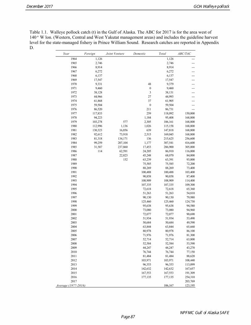
Table 1.1. Walleye pollock catch (t) in the Gulf of Alaska. The ABC for 2017 is for the area west of 140 o W lon. (Western, Central and West Yakutat management areas) and includes the guideline harvest level for the state-managed fishery in Prince William Sound. Research catches are reported in Appendix D.

Year Foreign Joint Venture Domestic Total ABC/TAC1964 1,126 1,126 ---1965 2,746 2,746 ---1966 8,914 8,914 ---1967 6,272 6,272 ---1968 6,137 6,137 ---1969 17,547 17,547 ---1970 9,331 48 9,379 ---1971 9,460 0 9,460 ---1972 38,128 3 38,131 ---1973 44,966 27 44,993 ---1974 61,868 37 61,905 ---1975 59,504 0 59,504 ---1976 86,520 211 86,731 ---1977 117,833 259 118,092 150,0001978 94,223 1,184 95,408 168,8001979 103,278 577 2,305 106,161 168,8001980 112,996 1,136 1,026 115,158 168,8001981 130,323 16,856 639 147,818 168,8001982 92,612 73,918 2,515 169,045 168,8001983 81,318 134,171 136 215,625 256,6001984 99,259 207,104 1,177 307,541 416,6001985 31,587 237,860 17,453 286,900 305,0001986 114 62,591 24,205 86,910 116,0001987 22,823 45,248 68,070 84,0001988 152 63,239 63,391 93,0001989 75,585 75,585 72,2001990 88,269 88,269 73,4001991 100,488 100,488 103,4001992 90,858 90,858 87,4001993 108,909 108,909 114,4001994 107,335 107,335 109,3001995 72,618 72,618 65,3601996 51,263 51,263 54,8101997 90,130 90,130 79,9801998 125,460 125,460 124,7301999 95,638 95,638 94,5802000 73,080 73,080 94,9602001 72,077 72,077 90,6902002 51,934 51,934 53,4902003 50,684 50,684 49,5902004 63,844 63,844 65,6602005 80,978 80,978 86,1002006 71,976 71,976 81,3002007 52,714 52,714 63,8002008 52,584 52,584 53,5902009 44,247 44,247 43,2702010 76,744 76,744 77,1502011 81,484 81,484 88,6202012 103,971 103,971 108,4402013 96,353 96,353 113,0992014 142,632 142,632 167,6572015 167,553 167,553 191,3092016 177,135 177,135 254,3102017 203,769

Average (1977-2016) 106,167 123,195

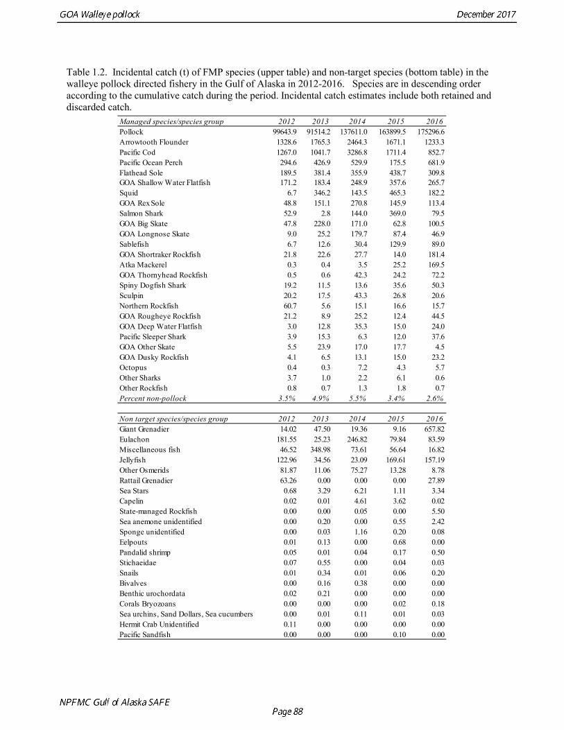
Table 1.2. Incidental catch (t) of FMP species (upper table) and non-target species (bottom table) in the walleye pollock directed fishery in the Gulf of Alaska in 2012-2016. Species are in descending order according to the cumulative catch during the period. Incidental catch estimates include both retained and discarded catch.

Managed species/species group 2012 2013 2014 2015 2016Pollock 99643.9 91514.2 137611.0 163899.5 175296.6Arrowtooth Flounder 1328.6 1765.3 2464.3 1671.1 1233.3Pacific Cod 1267.0 1041.7 3286.8 1711.4 852.7Pacific Ocean Perch 294.6 426.9 529.9 175.5 681.9Flathead Sole 189.5 381.4 355.9 438.7 309.8GOA Shallow Water Flatfish 171.2 183.4 248.9 357.6 265.7Squid 6.7 346.2 143.5 465.3 182.2GOA Rex Sole 48.8 151.1 270.8 145.9 113.4Salmon Shark 52.9 2.8 144.0 369.0 79.5GOA Big Skate 47.8 228.0 171.0 62.8 100.5GOA Longnose Skate 9.0 25.2 179.7 87.4 46.9Sablefish 6.7 12.6 30.4 129.9 89.0GOA Shortraker Rockfish 21.8 22.6 27.7 14.0 181.4Atka Mackerel 0.3 0.4 3.5 25.2 169.5GOA Thornyhead Rockfish 0.5 0.6 42.3 24.2 72.2Spiny Dogfish Shark 19.2 11.5 13.6 35.6 50.3Sculpin 20.2 17.5 43.3 26.8 20.6Northern Rockfish 60.7 5.6 15.1 16.6 15.7GOA Rougheye Rockfish 21.2 8.9 25.2 12.4 44.5GOA Deep Water Flatfish 3.0 12.8 35.3 15.0 24.0Pacific Sleeper Shark 3.9 15.3 6.3 12.0 37.6GOA Other Skate 5.5 23.9 17.0 17.7 4.5GOA Dusky Rockfish 4.1 6.5 13.1 15.0 23.2Octopus 0.4 0.3 7.2 4.3 5.7Other Sharks 3.7 1.0 2.2 6.1 0.6Other Rockfish 0.8 0.7 1.3 1.8 0.7Percent non-pollock 3.5% 4.9% 5.5% 3.4% 2.6%

Non target species/species group 2012 2013 2014 2015 2016Giant Grenadier 14.02 47.50 19.36 9.16 657.82Eulachon 181.55 25.23 246.82 79.84 83.59Miscellaneous fish 46.52 348.98 73.61 56.64 16.82Jellyfish 122.96 34.56 23.09 169.61 157.19Other Osmerids 81.87 11.06 75.27 13.28 8.78Rattail Grenadier 63.26 0.00 0.00 0.00 27.89Sea Stars 0.68 3.29 6.21 1.11 3.34Capelin 0.02 0.01 4.61 3.62 0.02State-managed Rockfish 0.00 0.00 0.05 0.00 5.50Sea anemone unidentified 0.00 0.20 0.00 0.55 2.42Sponge unidentified 0.00 0.03 1.16 0.20 0.08Eelpouts 0.01 0.13 0.00 0.68 0.00Pandalid shrimp 0.05 0.01 0.04 0.17 0.50Stichaeidae 0.07 0.55 0.00 0.04 0.03Snails 0.01 0.34 0.01 0.06 0.20Bivalves 0.00 0.16 0.38 0.00 0.00Benthic urochordata 0.02 0.21 0.00 0.00 0.00Corals Bryozoans 0.00 0.00 0.00 0.02 0.18Sea urchins, Sand Dollars, Sea cucumbers 0.00 0.01 0.11 0.01 0.03Hermit Crab Unidentified 0.11 0.00 0.00 0.00 0.00Pacific Sandfish 0.00 0.00 0.00 0.10 0.00

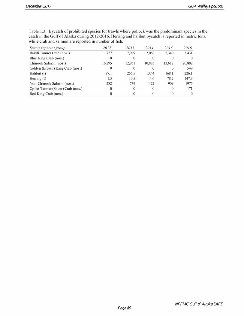
Table 1.3. Bycatch of prohibited species for trawls where pollock was the predominant species in the catch in the Gulf of Alaska during 2012-2016. Herring and halibut bycatch is reported in metric tons, while crab and salmon are reported in number of fish.

Species/species group 2012 2013 2014 2015 2016Bairdi Tanner Crab (nos.) 727 7,999 2,062 2,340 3,431Blue King Crab (nos.) 0 0 0 0 0Chinook Salmon (nos.) 16,295 12,951 10,883 13,612 20,882Golden (Brown) King Crab (nos.) 0 0 0 0 549Halibut (t) 87.1 256.5 137.4 168.1 226.1Herring (t) 1.3 10.5 4.6 78.2 147.3Non-Chinook Salmon (nos.) 282 739 1422 909 1975Opilio Tanner (Snow) Crab (nos.) 0 0 0 0 171Red King Crab (nos.) 0 0 0 0 0

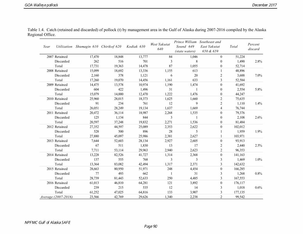
Table 1.4. Catch (retained and discarded) of pollock (t) by management area in the Gulf of Alaska during 2007-2016 compiled by the Alaska Regional Office.

Year Utilization Shumagin 610 Chirikof 620 Kodiak 630 West Yakutat 640

Prince William Sound 649

(state waters)

Southeast and East Yakutat 650 & 659

Total Percent discard

2007 Retained 17,470 18,848 13,777 84 1,046 0 51,224Discarded 262 516 701 3 8 0 1,490 2.8%Total 17,731 19,363 14,478 87 1,055 0 52,714

2008 Retained 15,099 18,692 13,336 1,155 613 1 48,896Discarded 2,160 378 1,121 6 20 2 3,688 7.0%Total 17,260 19,070 14,456 1,161 633 3 52,584

2009 Retained 14,475 13,578 10,974 1,190 1,474 0 41,692Discarded 604 422 1,496 31 1 0 2,554 5.8%Total 15,079 14,000 12,470 1,222 1,476 0 44,247

2010 Retained 25,960 28,015 18,373 1,625 1,660 2 75,635Discarded 91 234 761 12 9 2 1,110 1.4%Total 26,051 28,249 19,134 1,637 1,669 4 76,744

2011 Retained 20,472 36,114 18,987 2,268 1,535 0 79,376Discarded 125 1,134 844 3 1 0 2,108 2.6%Total 20,597 37,248 19,832 2,271 1,536 0 81,484

2012 Retained 27,352 44,597 25,089 2,353 2,622 0 102,012Discarded 528 500 896 28 5 1 1,959 1.9%Total 27,880 45,097 25,986 2,381 2,627 1 103,971

2013 Retained 7,644 52,603 28,134 2,927 2,605 0 93,913Discarded 67 511 1,830 13 17 2 2,440 2.5%Total 7,711 53,114 29,963 2,940 2,623 2 96,353

2014 Retained 13,228 82,526 41,727 1,314 2,368 0 141,163Discarded 137 555 768 3 3 3 1,469 1.0%Total 13,364 83,082 42,494 1,317 2,371 3 142,632

2015 Retained 28,663 80,950 51,971 248 4,454 0 166,285Discarded 77 493 662 1 31 3 1,268 0.8%Total 28,739 81,443 52,633 250 4,485 3 167,553

2016 Retained 61,013 46,810 64,281 121 3,892 0 176,117Discarded 239 215 535 12 14 3 1,018 0.6%Total 61,252 47,025 64,816 133 3,907 3 177,135

Average (2007-2016) 23,566 42,769 29,626 1,340 2,238 2 99,542

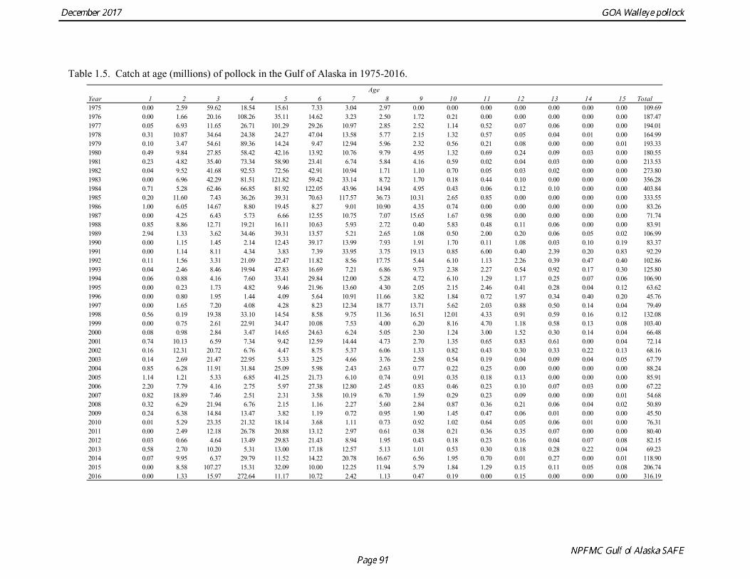
Table 1.5. Catch at age (millions) of pollock in the Gulf of Alaska in 1975-2016.

AgeYear 1 2 3 4 5 6 7 8 9 10 11 12 13 14 15 Total1975 0.00 2.59 59.62 18.54 15.61 7.33 3.04 2.97 0.00 0.00 0.00 0.00 0.00 0.00 0.00 109.691976 0.00 1.66 20.16 108.26 35.11 14.62 3.23 2.50 1.72 0.21 0.00 0.00 0.00 0.00 0.00 187.471977 0.05 6.93 11.65 26.71 101.29 29.26 10.97 2.85 2.52 1.14 0.52 0.07 0.06 0.00 0.00 194.011978 0.31 10.87 34.64 24.38 24.27 47.04 13.58 5.77 2.15 1.32 0.57 0.05 0.04 0.01 0.00 164.991979 0.10 3.47 54.61 89.36 14.24 9.47 12.94 5.96 2.32 0.56 0.21 0.08 0.00 0.00 0.01 193.331980 0.49 9.84 27.85 58.42 42.16 13.92 10.76 9.79 4.95 1.32 0.69 0.24 0.09 0.03 0.00 180.551981 0.23 4.82 35.40 73.34 58.90 23.41 6.74 5.84 4.16 0.59 0.02 0.04 0.03 0.00 0.00 213.531982 0.04 9.52 41.68 92.53 72.56 42.91 10.94 1.71 1.10 0.70 0.05 0.03 0.02 0.00 0.00 273.801983 0.00 6.96 42.29 81.51 121.82 59.42 33.14 8.72 1.70 0.18 0.44 0.10 0.00 0.00 0.00 356.281984 0.71 5.28 62.46 66.85 81.92 122.05 43.96 14.94 4.95 0.43 0.06 0.12 0.10 0.00 0.00 403.841985 0.20 11.60 7.43 36.26 39.31 70.63 117.57 36.73 10.31 2.65 0.85 0.00 0.00 0.00 0.00 333.551986 1.00 6.05 14.67 8.80 19.45 8.27 9.01 10.90 4.35 0.74 0.00 0.00 0.00 0.00 0.00 83.261987 0.00 4.25 6.43 5.73 6.66 12.55 10.75 7.07 15.65 1.67 0.98 0.00 0.00 0.00 0.00 71.741988 0.85 8.86 12.71 19.21 16.11 10.63 5.93 2.72 0.40 5.83 0.48 0.11 0.06 0.00 0.00 83.911989 2.94 1.33 3.62 34.46 39.31 13.57 5.21 2.65 1.08 0.50 2.00 0.20 0.06 0.05 0.02 106.991990 0.00 1.15 1.45 2.14 12.43 39.17 13.99 7.93 1.91 1.70 0.11 1.08 0.03 0.10 0.19 83.371991 0.00 1.14 8.11 4.34 3.83 7.39 33.95 3.75 19.13 0.85 6.00 0.40 2.39 0.20 0.83 92.291992 0.11 1.56 3.31 21.09 22.47 11.82 8.56 17.75 5.44 6.10 1.13 2.26 0.39 0.47 0.40 102.861993 0.04 2.46 8.46 19.94 47.83 16.69 7.21 6.86 9.73 2.38 2.27 0.54 0.92 0.17 0.30 125.801994 0.06 0.88 4.16 7.60 33.41 29.84 12.00 5.28 4.72 6.10 1.29 1.17 0.25 0.07 0.06 106.901995 0.00 0.23 1.73 4.82 9.46 21.96 13.60 4.30 2.05 2.15 2.46 0.41 0.28 0.04 0.12 63.621996 0.00 0.80 1.95 1.44 4.09 5.64 10.91 11.66 3.82 1.84 0.72 1.97 0.34 0.40 0.20 45.761997 0.00 1.65 7.20 4.08 4.28 8.23 12.34 18.77 13.71 5.62 2.03 0.88 0.50 0.14 0.04 79.491998 0.56 0.19 19.38 33.10 14.54 8.58 9.75 11.36 16.51 12.01 4.33 0.91 0.59 0.16 0.12 132.081999 0.00 0.75 2.61 22.91 34.47 10.08 7.53 4.00 6.20 8.16 4.70 1.18 0.58 0.13 0.08 103.402000 0.08 0.98 2.84 3.47 14.65 24.63 6.24 5.05 2.30 1.24 3.00 1.52 0.30 0.14 0.04 66.482001 0.74 10.13 6.59 7.34 9.42 12.59 14.44 4.73 2.70 1.35 0.65 0.83 0.61 0.00 0.04 72.142002 0.16 12.31 20.72 6.76 4.47 8.75 5.37 6.06 1.33 0.82 0.43 0.30 0.33 0.22 0.13 68.162003 0.14 2.69 21.47 22.95 5.33 3.25 4.66 3.76 2.58 0.54 0.19 0.04 0.09 0.04 0.05 67.792004 0.85 6.28 11.91 31.84 25.09 5.98 2.43 2.63 0.77 0.22 0.25 0.00 0.00 0.00 0.00 88.242005 1.14 1.21 5.33 6.85 41.25 21.73 6.10 0.74 0.91 0.35 0.18 0.13 0.00 0.00 0.00 85.912006 2.20 7.79 4.16 2.75 5.97 27.38 12.80 2.45 0.83 0.46 0.23 0.10 0.07 0.03 0.00 67.222007 0.82 18.89 7.46 2.51 2.31 3.58 10.19 6.70 1.59 0.29 0.23 0.09 0.00 0.00 0.01 54.682008 0.32 6.29 21.94 6.76 2.15 1.16 2.27 5.60 2.84 0.87 0.36 0.21 0.06 0.04 0.02 50.892009 0.24 6.38 14.84 13.47 3.82 1.19 0.72 0.95 1.90 1.45 0.47 0.06 0.01 0.00 0.00 45.502010 0.01 5.29 23.35 21.32 18.14 3.68 1.11 0.73 0.92 1.02 0.64 0.05 0.06 0.01 0.00 76.312011 0.00 2.49 12.18 26.78 20.88 13.12 2.97 0.61 0.38 0.21 0.36 0.35 0.07 0.00 0.00 80.402012 0.03 0.66 4.64 13.49 29.83 21.43 8.94 1.95 0.43 0.18 0.23 0.16 0.04 0.07 0.08 82.152013 0.58 2.70 10.20 5.31 13.00 17.18 12.57 5.13 1.01 0.53 0.30 0.18 0.28 0.22 0.04 69.232014 0.07 9.95 6.37 29.79 11.52 14.22 20.78 16.67 6.56 1.95 0.70 0.01 0.27 0.00 0.01 118.902015 0.00 8.58 107.27 15.31 32.09 10.00 12.25 11.94 5.79 1.84 1.29 0.15 0.11 0.05 0.08 206.742016 0.00 1.33 15.97 272.64 11.17 10.72 2.42 1.13 0.47 0.19 0.00 0.15 0.00 0.00 0.00 316.19

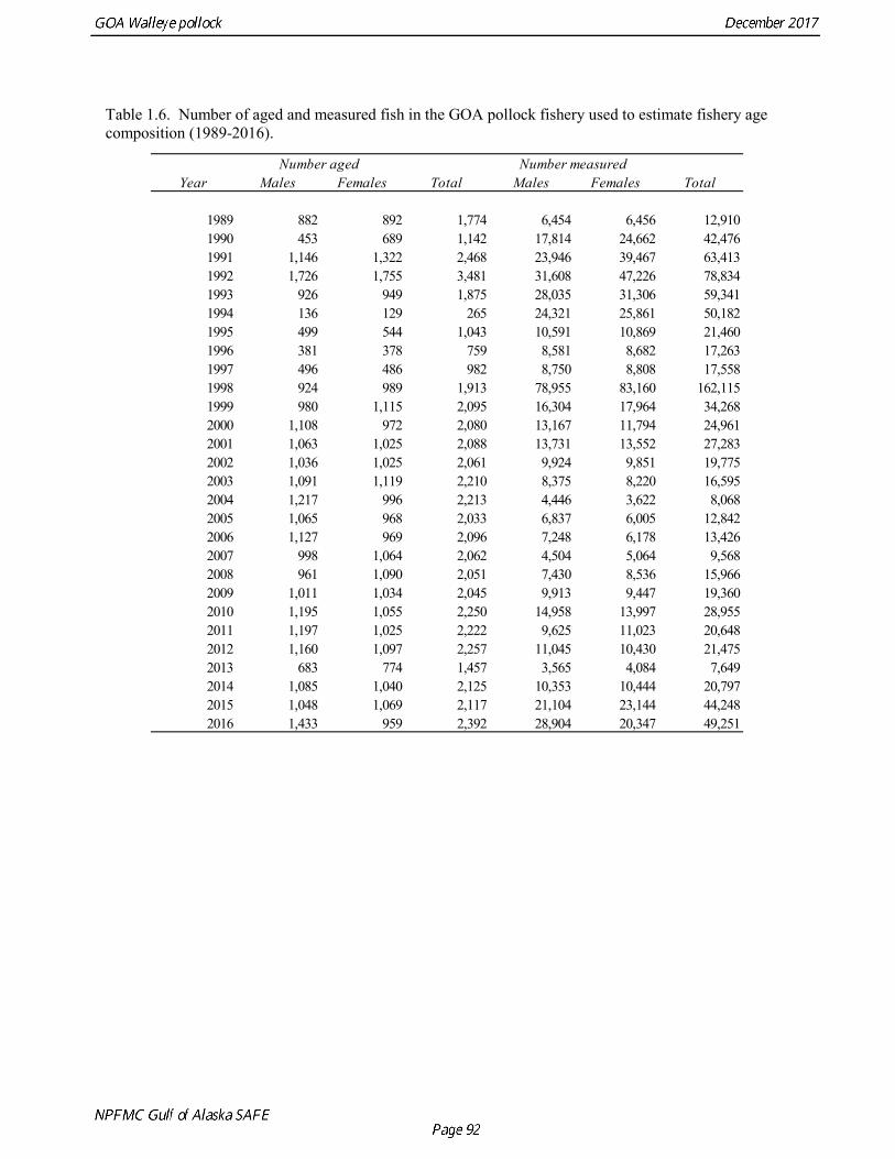
Table 1.6. Number of aged and measured fish in the GOA pollock fishery used to estimate fishery age composition (1989-2016).

Year Males Females Total Males Females Total

1989 882 892 1,774 6,454 6,456 12,9101990 453 689 1,142 17,814 24,662 42,4761991 1,146 1,322 2,468 23,946 39,467 63,4131992 1,726 1,755 3,481 31,608 47,226 78,8341993 926 949 1,875 28,035 31,306 59,3411994 136 129 265 24,321 25,861 50,1821995 499 544 1,043 10,591 10,869 21,4601996 381 378 759 8,581 8,682 17,2631997 496 486 982 8,750 8,808 17,5581998 924 989 1,913 78,955 83,160 162,1151999 980 1,115 2,095 16,304 17,964 34,2682000 1,108 972 2,080 13,167 11,794 24,9612001 1,063 1,025 2,088 13,731 13,552 27,2832002 1,036 1,025 2,061 9,924 9,851 19,7752003 1,091 1,119 2,210 8,375 8,220 16,5952004 1,217 996 2,213 4,446 3,622 8,0682005 1,065 968 2,033 6,837 6,005 12,8422006 1,127 969 2,096 7,248 6,178 13,4262007 998 1,064 2,062 4,504 5,064 9,5682008 961 1,090 2,051 7,430 8,536 15,9662009 1,011 1,034 2,045 9,913 9,447 19,3602010 1,195 1,055 2,250 14,958 13,997 28,9552011 1,197 1,025 2,222 9,625 11,023 20,6482012 1,160 1,097 2,257 11,045 10,430 21,4752013 683 774 1,457 3,565 4,084 7,6492014 1,085 1,040 2,125 10,353 10,444 20,7972015 1,048 1,069 2,117 21,104 23,144 44,2482016 1,433 959 2,392 28,904 20,347 49,251

Number measuredNumber aged

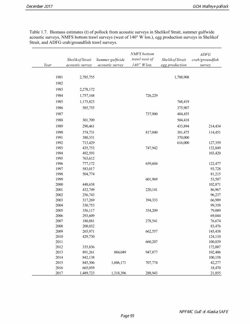
Table 1.7. Biomass estimates (t) of pollock from acoustic surveys in Shelikof Strait, summer gulfwide acoustic surveys, NMFS bottom trawl surveys (west of 140° W lon.), egg production surveys in Shelikof Strait, and ADFG crab/groundfish trawl surveys.

1981 2,785,755 1,788,90819821983 2,278,1721984 1,757,168 726,2291985 1,175,823 768,4191986 585,755 375,9071987 737,900 484,4551988 301,709 504,4181989 290,461 433,894 214,4341990 374,731 817,040 381,475 114,4511991 380,331 370,0001992 713,429 616,000 127,3591993 435,753 747,942 132,8491994 492,593 103,4201995 763,6121996 777,172 659,604 122,4771997 583,017 93,7281998 504,774 81,2151999 601,969 53,5872000 448,638 102,8712001 432,749 220,141 86,9672002 256,743 96,2372003 317,269 394,333 66,9892004 330,753 99,3582005 356,117 354,209 79,0892006 293,609 69,0442007 180,881 278,541 76,6742008 208,032 83,4762009 265,971 662,557 145,4382010 429,730 124,1102011 660,207 100,8392012 335,836 172,0072013 891,261 884,049 947,877 102,4062014 842,138 100,1582015 845,306 1,606,171 707,774 42,2772016 665,059 18,4702017 1,489,723 1,318,396 288,943 21,855

ADFG crab/groundfish

surveyYearShelikof Strait acoustic survey

Summer gulfwide acoustic survey

NMFS bottom trawl west of 140 o W lon.

Shelikof Strait egg production

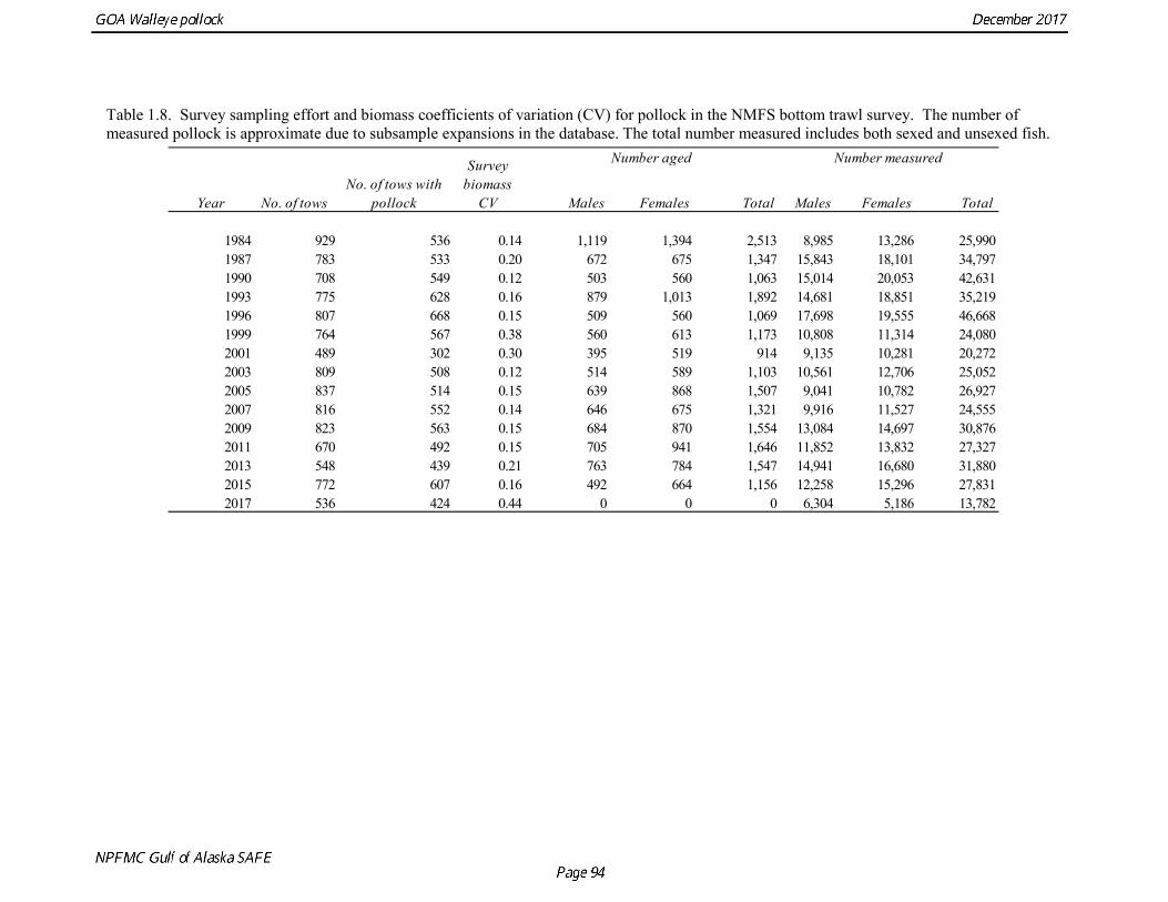
Table 1.8. Survey sampling effort and biomass coefficients of variation (CV) for pollock in the NMFS bottom trawl survey. The number of measured pollock is approximate due to subsample expansions in the database. The total number measured includes both sexed and unsexed fish.

Year Males Females Total Males Females Total

1984 929 536 0.14 1,119 1,394 2,513 8,985 13,286 25,9901987 783 533 0.20 672 675 1,347 15,843 18,101 34,7971990 708 549 0.12 503 560 1,063 15,014 20,053 42,6311993 775 628 0.16 879 1,013 1,892 14,681 18,851 35,2191996 807 668 0.15 509 560 1,069 17,698 19,555 46,6681999 764 567 0.38 560 613 1,173 10,808 11,314 24,0802001 489 302 0.30 395 519 914 9,135 10,281 20,2722003 809 508 0.12 514 589 1,103 10,561 12,706 25,0522005 837 514 0.15 639 868 1,507 9,041 10,782 26,9272007 816 552 0.14 646 675 1,321 9,916 11,527 24,5552009 823 563 0.15 684 870 1,554 13,084 14,697 30,8762011 670 492 0.15 705 941 1,646 11,852 13,832 27,3272013 548 439 0.21 763 784 1,547 14,941 16,680 31,8802015 772 607 0.16 492 664 1,156 12,258 15,296 27,8312017 536 424 0.44 0 0 0 6,304 5,186 13,782

Number measured

No. of tows

Survey biomass

CVNo. of tows with

pollock

Number aged

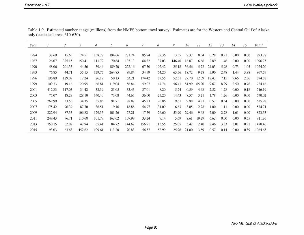
Table 1.9. Estimated number at age (millions) from the NMFS bottom trawl survey. Estimates are for the Western and Central Gulf of Alaska only (statistical areas 610-630).

Year 1 2 3 4 5 6 7 8 9 10 11 12 13 14 15 Total

1984 38.69 15.65 74.51 158.78 194.66 271.24 85.94 37.36 13.55 2.37 0.54 0.28 0.21 0.00 0.00 893.781987 26.07 325.15 150.41 111.72 70.64 135.13 64.32 37.03 146.40 18.87 6.66 2.89 1.46 0.00 0.00 1096.751990 58.06 201.33 44.56 39.44 189.70 222.16 67.30 102.42 25.18 36.56 5.72 24.03 5.98 0.73 1.05 1024.201993 76.85 44.71 55.15 129.75 264.85 89.84 34.99 64.20 65.56 18.72 9.28 5.90 2.48 1.44 3.88 867.591996 196.89 129.07 17.24 26.17 50.13 63.21 174.42 87.55 52.31 27.70 12.09 18.43 7.15 9.66 2.86 874.881999 109.73 19.16 20.95 66.81 119.04 56.84 59.07 47.74 56.41 81.99 65.20 9.67 8.29 2.50 0.76 724.162001 412.83 117.03 34.42 33.39 25.05 33.45 37.01 8.20 5.74 0.59 4.48 2.52 1.28 0.00 0.18 716.192003 75.07 18.29 128.10 140.40 73.08 44.63 36.00 25.20 14.43 8.57 3.21 1.78 1.26 0.00 0.00 570.022005 269.99 33.56 34.35 35.85 91.71 78.82 45.23 20.86 9.61 9.98 4.81 0.57 0.64 0.00 0.00 635.982007 175.42 96.39 87.70 36.51 19.16 18.88 54.97 31.09 6.63 3.05 2.78 1.00 1.11 0.00 0.00 534.712009 222.94 87.33 106.82 129.35 101.26 27.21 17.59 26.60 53.90 29.46 9.68 7.00 2.78 1.61 0.00 823.532011 249.43 96.71 110.68 101.79 163.62 107.99 33.24 7.14 5.69 8.61 19.29 6.62 0.00 0.00 0.55 911.362013 750.15 62.07 47.94 65.41 84.72 144.62 156.91 115.55 25.05 5.42 2.40 2.46 3.83 3.01 0.91 1470.462015 93.03 63.63 452.62 109.61 113.20 70.83 56.57 52.99 25.96 21.00 3.59 0.57 0.14 0.00 0.89 1064.65

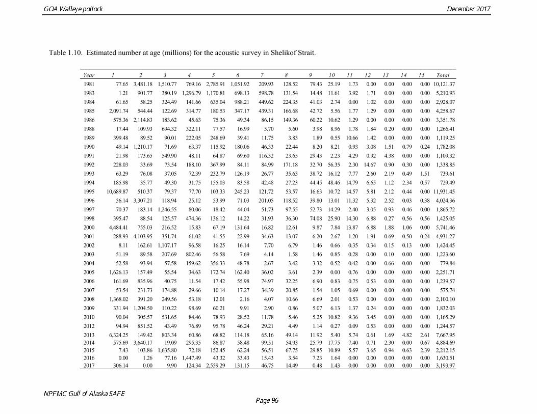
Table 1.10. Estimated number at age (millions) for the acoustic survey in Shelikof Strait.

Year 1 2 3 4 5 6 7 8 9 10 11 12 13 14 15 Total1981 77.65 3,481.18 1,510.77 769.16 2,785.91 1,051.92 209.93 128.52 79.43 25.19 1.73 0.00 0.00 0.00 0.00 10,121.371983 1.21 901.77 380.19 1,296.79 1,170.81 698.13 598.78 131.54 14.48 11.61 3.92 1.71 0.00 0.00 0.00 5,210.931984 61.65 58.25 324.49 141.66 635.04 988.21 449.62 224.35 41.03 2.74 0.00 1.02 0.00 0.00 0.00 2,928.071985 2,091.74 544.44 122.69 314.77 180.53 347.17 439.31 166.68 42.72 5.56 1.77 1.29 0.00 0.00 0.00 4,258.671986 575.36 2,114.83 183.62 45.63 75.36 49.34 86.15 149.36 60.22 10.62 1.29 0.00 0.00 0.00 0.00 3,351.781988 17.44 109.93 694.32 322.11 77.57 16.99 5.70 5.60 3.98 8.96 1.78 1.84 0.20 0.00 0.00 1,266.411989 399.48 89.52 90.01 222.05 248.69 39.41 11.75 3.83 1.89 0.55 10.66 1.42 0.00 0.00 0.00 1,119.251990 49.14 1,210.17 71.69 63.37 115.92 180.06 46.33 22.44 8.20 8.21 0.93 3.08 1.51 0.79 0.24 1,782.081991 21.98 173.65 549.90 48.11 64.87 69.60 116.32 23.65 29.43 2.23 4.29 0.92 4.38 0.00 0.00 1,109.321992 228.03 33.69 73.54 188.10 367.99 84.11 84.99 171.18 32.70 56.35 2.30 14.67 0.90 0.30 0.00 1,338.851993 63.29 76.08 37.05 72.39 232.79 126.19 26.77 35.63 38.72 16.12 7.77 2.60 2.19 0.49 1.51 739.611994 185.98 35.77 49.30 31.75 155.03 83.58 42.48 27.23 44.45 48.46 14.79 6.65 1.12 2.34 0.57 729.491995 10,689.87 510.37 79.37 77.70 103.33 245.23 121.72 53.57 16.63 10.72 14.57 5.81 2.12 0.44 0.00 11,931.451996 56.14 3,307.21 118.94 25.12 53.99 71.03 201.05 118.52 39.80 13.01 11.32 5.32 2.52 0.03 0.38 4,024.361997 70.37 183.14 1,246.55 80.06 18.42 44.04 51.73 97.55 52.73 14.29 2.40 3.05 0.93 0.46 0.00 1,865.721998 395.47 88.54 125.57 474.36 136.12 14.22 31.93 36.30 74.08 25.90 14.30 6.88 0.27 0.56 0.56 1,425.052000 4,484.41 755.03 216.52 15.83 67.19 131.64 16.82 12.61 9.87 7.84 13.87 6.88 1.88 1.06 0.00 5,741.462001 288.93 4,103.95 351.74 61.02 41.55 22.99 34.63 13.07 6.20 2.67 1.20 1.91 0.69 0.50 0.24 4,931.272002 8.11 162.61 1,107.17 96.58 16.25 16.14 7.70 6.79 1.46 0.66 0.35 0.34 0.15 0.13 0.00 1,424.452003 51.19 89.58 207.69 802.46 56.58 7.69 4.14 1.58 1.46 0.85 0.28 0.00 0.10 0.00 0.00 1,223.602004 52.58 93.94 57.58 159.62 356.33 48.78 2.67 3.42 3.32 0.52 0.42 0.00 0.66 0.00 0.00 779.842005 1,626.13 157.49 55.54 34.63 172.74 162.40 36.02 3.61 2.39 0.00 0.76 0.00 0.00 0.00 0.00 2,251.712006 161.69 835.96 40.75 11.54 17.42 55.98 74.97 32.25 6.90 0.83 0.75 0.53 0.00 0.00 0.00 1,239.572007 53.54 231.73 174.88 29.66 10.14 17.27 34.39 20.85 1.54 1.05 0.69 0.00 0.00 0.00 0.00 575.742008 1,368.02 391.20 249.56 53.18 12.01 2.16 4.07 10.66 6.69 2.01 0.53 0.00 0.00 0.00 0.00 2,100.102009 331.94 1,204.50 110.22 98.69 60.21 9.91 2.90 0.86 5.07 6.13 1.37 0.24 0.00 0.00 0.00 1,832.032010 90.04 305.57 531.65 84.46 78.93 28.52 11.78 5.46 5.25 10.82 9.36 3.45 0.00 0.00 0.00 1,165.292012 94.94 851.52 43.49 76.89 95.78 46.24 29.21 4.49 1.14 0.27 0.09 0.53 0.00 0.00 0.00 1,244.572013 6,324.25 149.42 803.34 60.86 68.82 114.18 65.16 49.14 11.92 5.40 5.74 0.61 1.69 4.82 2.61 7,667.952014 575.69 3,640.17 19.09 295.35 86.87 58.48 99.51 54.93 25.79 17.75 7.40 0.71 2.30 0.00 0.67 4,884.692015 7.43 103.86 1,635.80 72.18 152.45 62.24 56.51 67.75 29.85 10.89 5.57 3.65 0.94 0.63 2.39 2,212.152016 0.00 1.26 77.16 1,447.49 43.32 33.43 15.43 3.54 7.23 1.64 0.00 0.00 0.00 0.00 0.00 1,630.512017 306.14 0.00 9.90 124.34 2,559.29 131.15 46.75 14.49 0.48 1.43 0.00 0.00 0.00 0.00 0.00 3,193.97

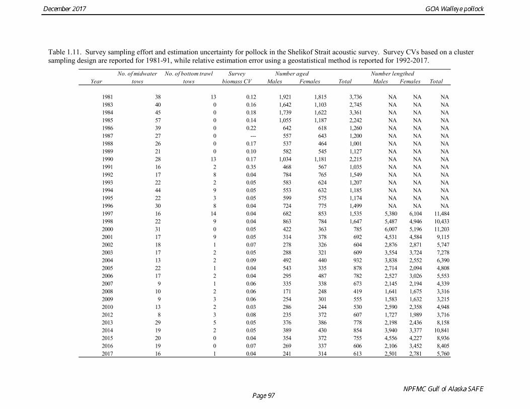
Table 1.11. Survey sampling effort and estimation uncertainty for pollock in the Shelikof Strait acoustic survey. Survey CVs based on a cluster sampling design are reported for 1981-91, while relative estimation error using a geostatistical method is reported for 1992-2017.

Year Males Females Total Males Females Total

1981 38 13 0.12 1,921 1,815 3,736 NA NA NA1983 40 0 0.16 1,642 1,103 2,745 NA NA NA1984 45 0 0.18 1,739 1,622 3,361 NA NA NA1985 57 0 0.14 1,055 1,187 2,242 NA NA NA1986 39 0 0.22 642 618 1,260 NA NA NA1987 27 0 --- 557 643 1,200 NA NA NA1988 26 0 0.17 537 464 1,001 NA NA NA1989 21 0 0.10 582 545 1,127 NA NA NA1990 28 13 0.17 1,034 1,181 2,215 NA NA NA1991 16 2 0.35 468 567 1,035 NA NA NA1992 17 8 0.04 784 765 1,549 NA NA NA1993 22 2 0.05 583 624 1,207 NA NA NA1994 44 9 0.05 553 632 1,185 NA NA NA1995 22 3 0.05 599 575 1,174 NA NA NA1996 30 8 0.04 724 775 1,499 NA NA NA1997 16 14 0.04 682 853 1,535 5,380 6,104 11,4841998 22 9 0.04 863 784 1,647 5,487 4,946 10,4332000 31 0 0.05 422 363 785 6,007 5,196 11,2032001 17 9 0.05 314 378 692 4,531 4,584 9,1152002 18 1 0.07 278 326 604 2,876 2,871 5,7472003 17 2 0.05 288 321 609 3,554 3,724 7,2782004 13 2 0.09 492 440 932 3,838 2,552 6,3902005 22 1 0.04 543 335 878 2,714 2,094 4,8082006 17 2 0.04 295 487 782 2,527 3,026 5,5532007 9 1 0.06 335 338 673 2,145 2,194 4,3392008 10 2 0.06 171 248 419 1,641 1,675 3,3162009 9 3 0.06 254 301 555 1,583 1,632 3,2152010 13 2 0.03 286 244 530 2,590 2,358 4,9482012 8 3 0.08 235 372 607 1,727 1,989 3,7162013 29 5 0.05 376 386 778 2,198 2,436 8,1582014 19 2 0.05 389 430 854 3,940 3,377 10,8412015 20 0 0.04 354 372 755 4,556 4,227 8,9362016 19 0 0.07 269 337 606 2,106 3,452 8,4052017 16 1 0.04 241 314 613 2,501 2,781 5,760

Number lengthedNo. of midwater tows

Survey biomass CV

No. of bottom trawl tows

Number aged

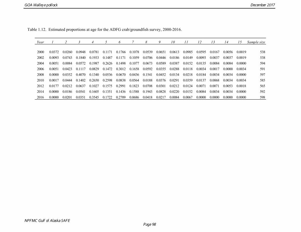
Table 1.12. Estimated proportions at age for the ADFG crab/groundfish survey, 2000-2016.

Year 1 2 3 4 5 6 7 8 9 10 11 12 13 14 15 Sample size

2000 0.0372 0.0260 0.0948 0.0781 0.1171 0.1766 0.1078 0.0539 0.0651 0.0613 0.0985 0.0595 0.0167 0.0056 0.0019 5382002 0.0093 0.0743 0.1840 0.1933 0.1487 0.1171 0.1059 0.0706 0.0446 0.0186 0.0149 0.0093 0.0037 0.0037 0.0019 5382004 0.0051 0.0084 0.0572 0.1987 0.2626 0.1498 0.1077 0.0673 0.0589 0.0387 0.0152 0.0135 0.0084 0.0084 0.0000 5942006 0.0051 0.0423 0.1117 0.0829 0.1472 0.3012 0.1658 0.0592 0.0355 0.0288 0.0118 0.0034 0.0017 0.0000 0.0034 5912008 0.0000 0.0352 0.4070 0.1340 0.0536 0.0670 0.0436 0.1541 0.0452 0.0134 0.0218 0.0184 0.0034 0.0034 0.0000 5972010 0.0017 0.0444 0.1402 0.2650 0.2598 0.0838 0.0564 0.0188 0.0376 0.0291 0.0359 0.0137 0.0068 0.0034 0.0034 5852012 0.0177 0.0212 0.0637 0.1027 0.1575 0.2991 0.1823 0.0708 0.0301 0.0212 0.0124 0.0071 0.0071 0.0053 0.0018 5652014 0.0000 0.0186 0.0541 0.1605 0.1351 0.1436 0.1588 0.1943 0.0828 0.0220 0.0152 0.0084 0.0034 0.0034 0.0000 5922016 0.0000 0.0201 0.0351 0.3545 0.1722 0.2709 0.0686 0.0418 0.0217 0.0084 0.0067 0.0000 0.0000 0.0000 0.0000 598

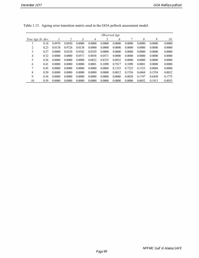
Table 1.13. Ageing error transition matrix used in the GOA pollock assessment model.

1 2 3 4 5 6 7 8 9 101 0.18 0.9970 0.0030 0.0000 0.0000 0.0000 0.0000 0.0000 0.0000 0.0000 0.00002 0.23 0.0138 0.9724 0.0138 0.0000 0.0000 0.0000 0.0000 0.0000 0.0000 0.00003 0.27 0.0000 0.0329 0.9342 0.0329 0.0000 0.0000 0.0000 0.0000 0.0000 0.00004 0.32 0.0000 0.0000 0.0571 0.8858 0.0571 0.0000 0.0000 0.0000 0.0000 0.00005 0.36 0.0000 0.0000 0.0000 0.0832 0.8335 0.0832 0.0000 0.0000 0.0000 0.00006 0.41 0.0000 0.0000 0.0000 0.0001 0.1090 0.7817 0.1090 0.0001 0.0000 0.00007 0.45 0.0000 0.0000 0.0000 0.0000 0.0004 0.1333 0.7325 0.1333 0.0004 0.00008 0.50 0.0000 0.0000 0.0000 0.0000 0.0000 0.0012 0.1554 0.6868 0.1554 0.00129 0.54 0.0000 0.0000 0.0000 0.0000 0.0000 0.0000 0.0028 0.1747 0.6450 0.177510 0.59 0.0000 0.0000 0.0000 0.0000 0.0000 0.0000 0.0000 0.0052 0.1913 0.8035

Observed AgeTrue Age St. dev.

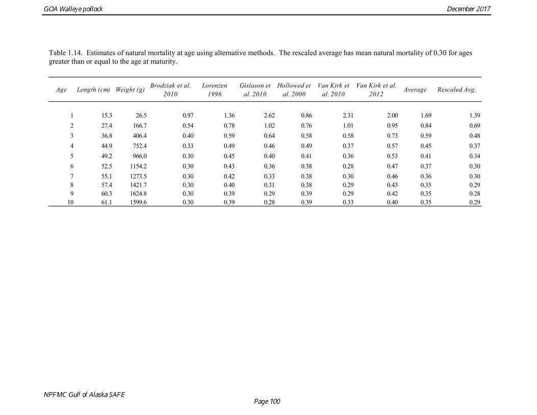
Table 1.14. Estimates of natural mortality at age using alternative methods. The rescaled average has mean natural mortality of 0.30 for ages greater than or equal to the age at maturity.

Age Length (cm) Weight (g) Brodziak et al. 2010

Lorenzen 1996

Gislason et al. 2010

Hollowed et al. 2000

Van Kirk et al. 2010

Van Kirk et al. 2012

Average Rescaled Avg.

1 15.3 26.5 0.97 1.36 2.62 0.86 2.31 2.00 1.69 1.392 27.4 166.7 0.54 0.78 1.02 0.76 1.01 0.95 0.84 0.693 36.8 406.4 0.40 0.59 0.64 0.58 0.58 0.73 0.59 0.484 44.9 752.4 0.33 0.49 0.46 0.49 0.37 0.57 0.45 0.375 49.2 966.0 0.30 0.45 0.40 0.41 0.36 0.53 0.41 0.346 52.5 1154.2 0.30 0.43 0.36 0.38 0.28 0.47 0.37 0.307 55.1 1273.5 0.30 0.42 0.33 0.38 0.30 0.46 0.36 0.308 57.4 1421.7 0.30 0.40 0.31 0.38 0.29 0.43 0.35 0.299 60.3 1624.8 0.30 0.39 0.29 0.39 0.29 0.42 0.35 0.28

10 61.1 1599.6 0.30 0.39 0.28 0.39 0.33 0.40 0.35 0.29

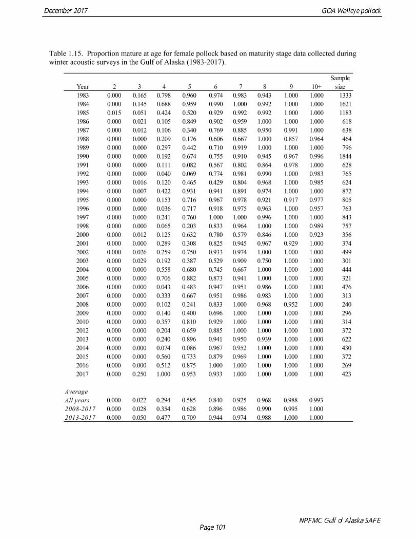
Table 1.15. Proportion mature at age for female pollock based on maturity stage data collected during winter acoustic surveys in the Gulf of Alaska (1983-2017).

Year 2 3 4 5 6 7 8 9 10+Sample

size1983 0.000 0.165 0.798 0.960 0.974 0.983 0.943 1.000 1.000 13331984 0.000 0.145 0.688 0.959 0.990 1.000 0.992 1.000 1.000 16211985 0.015 0.051 0.424 0.520 0.929 0.992 0.992 1.000 1.000 11831986 0.000 0.021 0.105 0.849 0.902 0.959 1.000 1.000 1.000 6181987 0.000 0.012 0.106 0.340 0.769 0.885 0.950 0.991 1.000 6381988 0.000 0.000 0.209 0.176 0.606 0.667 1.000 0.857 0.964 4641989 0.000 0.000 0.297 0.442 0.710 0.919 1.000 1.000 1.000 7961990 0.000 0.000 0.192 0.674 0.755 0.910 0.945 0.967 0.996 18441991 0.000 0.000 0.111 0.082 0.567 0.802 0.864 0.978 1.000 6281992 0.000 0.000 0.040 0.069 0.774 0.981 0.990 1.000 0.983 7651993 0.000 0.016 0.120 0.465 0.429 0.804 0.968 1.000 0.985 6241994 0.000 0.007 0.422 0.931 0.941 0.891 0.974 1.000 1.000 8721995 0.000 0.000 0.153 0.716 0.967 0.978 0.921 0.917 0.977 8051996 0.000 0.000 0.036 0.717 0.918 0.975 0.963 1.000 0.957 7631997 0.000 0.000 0.241 0.760 1.000 1.000 0.996 1.000 1.000 8431998 0.000 0.000 0.065 0.203 0.833 0.964 1.000 1.000 0.989 7572000 0.000 0.012 0.125 0.632 0.780 0.579 0.846 1.000 0.923 3562001 0.000 0.000 0.289 0.308 0.825 0.945 0.967 0.929 1.000 3742002 0.000 0.026 0.259 0.750 0.933 0.974 1.000 1.000 1.000 4992003 0.000 0.029 0.192 0.387 0.529 0.909 0.750 1.000 1.000 3012004 0.000 0.000 0.558 0.680 0.745 0.667 1.000 1.000 1.000 4442005 0.000 0.000 0.706 0.882 0.873 0.941 1.000 1.000 1.000 3212006 0.000 0.000 0.043 0.483 0.947 0.951 0.986 1.000 1.000 4762007 0.000 0.000 0.333 0.667 0.951 0.986 0.983 1.000 1.000 3132008 0.000 0.000 0.102 0.241 0.833 1.000 0.968 0.952 1.000 2402009 0.000 0.000 0.140 0.400 0.696 1.000 1.000 1.000 1.000 2962010 0.000 0.000 0.357 0.810 0.929 1.000 1.000 1.000 1.000 3142012 0.000 0.000 0.204 0.659 0.885 1.000 1.000 1.000 1.000 3722013 0.000 0.000 0.240 0.896 0.941 0.950 0.939 1.000 1.000 6222014 0.000 0.000 0.074 0.086 0.967 0.952 1.000 1.000 1.000 4302015 0.000 0.000 0.560 0.733 0.879 0.969 1.000 1.000 1.000 3722016 0.000 0.000 0.512 0.875 1.000 1.000 1.000 1.000 1.000 2692017 0.000 0.250 1.000 0.953 0.933 1.000 1.000 1.000 1.000 423

AverageAll years 0.000 0.022 0.294 0.585 0.840 0.925 0.968 0.988 0.9932008-2017 0.000 0.028 0.354 0.628 0.896 0.986 0.990 0.995 1.0002013-2017 0.000 0.050 0.477 0.709 0.944 0.974 0.988 1.000 1.000

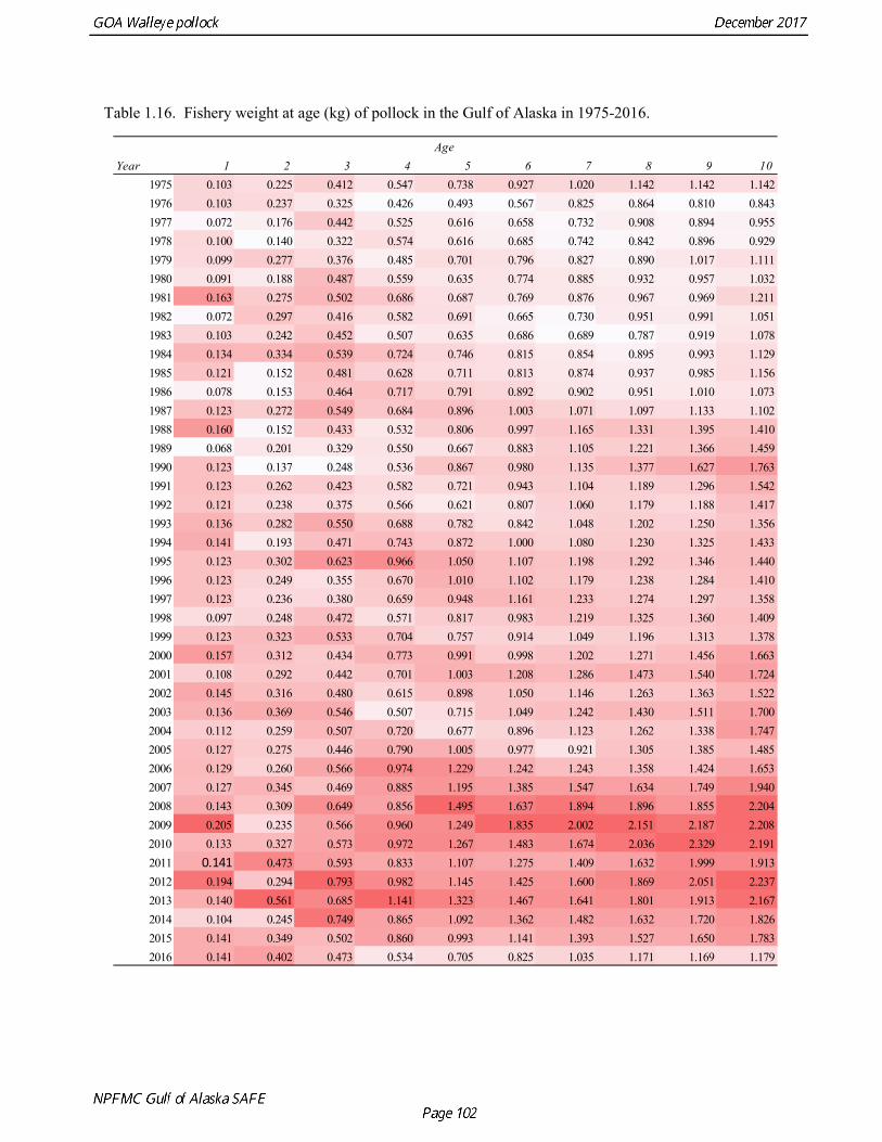
Table 1.16. Fishery weight at age (kg) of pollock in the Gulf of Alaska in 1975-2016.

AgeYear 1 2 3 4 5 6 7 8 9 10

1975 0.103 0.225 0.412 0.547 0.738 0.927 1.020 1.142 1.142 1.1421976 0.103 0.237 0.325 0.426 0.493 0.567 0.825 0.864 0.810 0.8431977 0.072 0.176 0.442 0.525 0.616 0.658 0.732 0.908 0.894 0.9551978 0.100 0.140 0.322 0.574 0.616 0.685 0.742 0.842 0.896 0.9291979 0.099 0.277 0.376 0.485 0.701 0.796 0.827 0.890 1.017 1.1111980 0.091 0.188 0.487 0.559 0.635 0.774 0.885 0.932 0.957 1.0321981 0.163 0.275 0.502 0.686 0.687 0.769 0.876 0.967 0.969 1.2111982 0.072 0.297 0.416 0.582 0.691 0.665 0.730 0.951 0.991 1.0511983 0.103 0.242 0.452 0.507 0.635 0.686 0.689 0.787 0.919 1.0781984 0.134 0.334 0.539 0.724 0.746 0.815 0.854 0.895 0.993 1.1291985 0.121 0.152 0.481 0.628 0.711 0.813 0.874 0.937 0.985 1.1561986 0.078 0.153 0.464 0.717 0.791 0.892 0.902 0.951 1.010 1.0731987 0.123 0.272 0.549 0.684 0.896 1.003 1.071 1.097 1.133 1.1021988 0.160 0.152 0.433 0.532 0.806 0.997 1.165 1.331 1.395 1.4101989 0.068 0.201 0.329 0.550 0.667 0.883 1.105 1.221 1.366 1.4591990 0.123 0.137 0.248 0.536 0.867 0.980 1.135 1.377 1.627 1.7631991 0.123 0.262 0.423 0.582 0.721 0.943 1.104 1.189 1.296 1.5421992 0.121 0.238 0.375 0.566 0.621 0.807 1.060 1.179 1.188 1.4171993 0.136 0.282 0.550 0.688 0.782 0.842 1.048 1.202 1.250 1.3561994 0.141 0.193 0.471 0.743 0.872 1.000 1.080 1.230 1.325 1.4331995 0.123 0.302 0.623 0.966 1.050 1.107 1.198 1.292 1.346 1.4401996 0.123 0.249 0.355 0.670 1.010 1.102 1.179 1.238 1.284 1.4101997 0.123 0.236 0.380 0.659 0.948 1.161 1.233 1.274 1.297 1.3581998 0.097 0.248 0.472 0.571 0.817 0.983 1.219 1.325 1.360 1.4091999 0.123 0.323 0.533 0.704 0.757 0.914 1.049 1.196 1.313 1.3782000 0.157 0.312 0.434 0.773 0.991 0.998 1.202 1.271 1.456 1.6632001 0.108 0.292 0.442 0.701 1.003 1.208 1.286 1.473 1.540 1.7242002 0.145 0.316 0.480 0.615 0.898 1.050 1.146 1.263 1.363 1.5222003 0.136 0.369 0.546 0.507 0.715 1.049 1.242 1.430 1.511 1.7002004 0.112 0.259 0.507 0.720 0.677 0.896 1.123 1.262 1.338 1.7472005 0.127 0.275 0.446 0.790 1.005 0.977 0.921 1.305 1.385 1.4852006 0.129 0.260 0.566 0.974 1.229 1.242 1.243 1.358 1.424 1.6532007 0.127 0.345 0.469 0.885 1.195 1.385 1.547 1.634 1.749 1.9402008 0.143 0.309 0.649 0.856 1.495 1.637 1.894 1.896 1.855 2.2042009 0.205 0.235 0.566 0.960 1.249 1.835 2.002 2.151 2.187 2.2082010 0.133 0.327 0.573 0.972 1.267 1.483 1.674 2.036 2.329 2.1912011 0.141 0.473 0.593 0.833 1.107 1.275 1.409 1.632 1.999 1.9132012 0.194 0.294 0.793 0.982 1.145 1.425 1.600 1.869 2.051 2.2372013 0.140 0.561 0.685 1.141 1.323 1.467 1.641 1.801 1.913 2.1672014 0.104 0.245 0.749 0.865 1.092 1.362 1.482 1.632 1.720 1.8262015 0.141 0.349 0.502 0.860 0.993 1.141 1.393 1.527 1.650 1.7832016 0.141 0.402 0.473 0.534 0.705 0.825 1.035 1.171 1.169 1.179

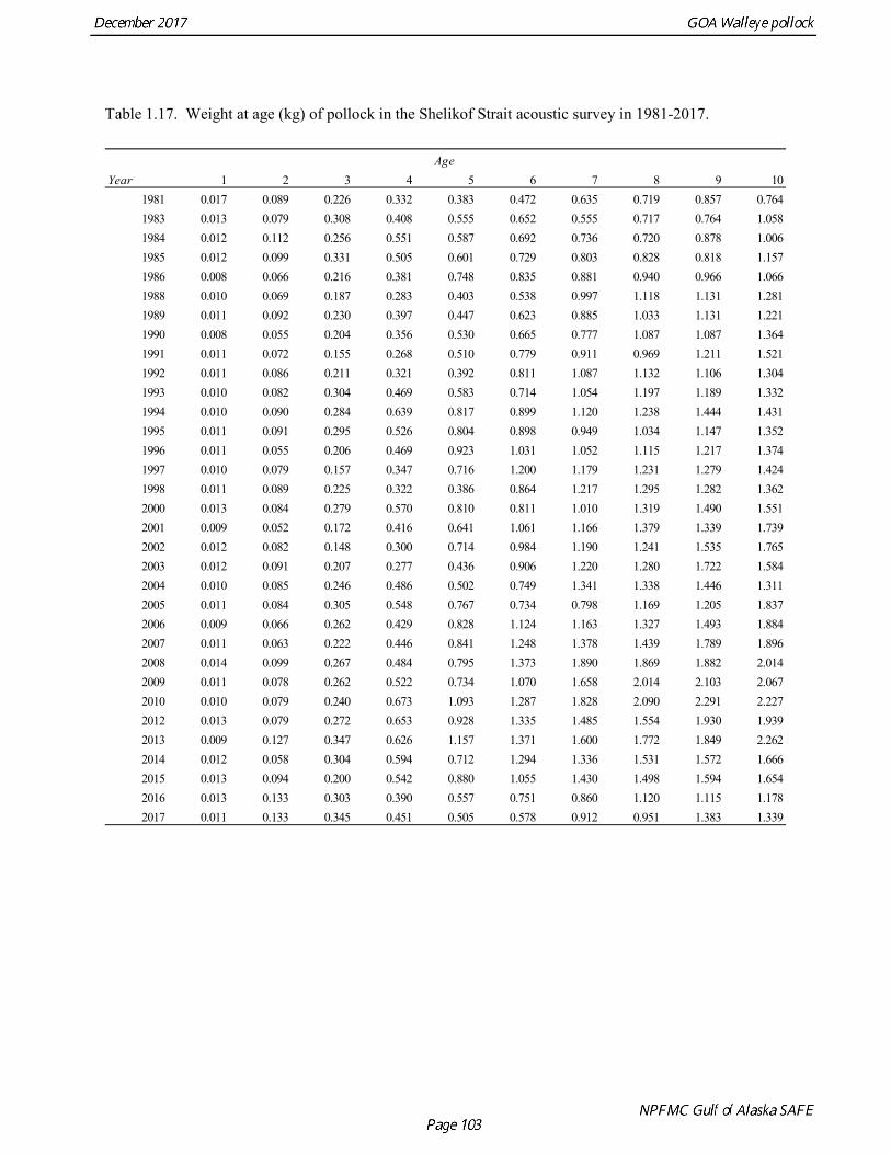
Table 1.17. Weight at age (kg) of pollock in the Shelikof Strait acoustic survey in 1981-2017.

AgeYear 1 2 3 4 5 6 7 8 9 10

1981 0.017 0.089 0.226 0.332 0.383 0.472 0.635 0.719 0.857 0.7641983 0.013 0.079 0.308 0.408 0.555 0.652 0.555 0.717 0.764 1.0581984 0.012 0.112 0.256 0.551 0.587 0.692 0.736 0.720 0.878 1.0061985 0.012 0.099 0.331 0.505 0.601 0.729 0.803 0.828 0.818 1.1571986 0.008 0.066 0.216 0.381 0.748 0.835 0.881 0.940 0.966 1.0661988 0.010 0.069 0.187 0.283 0.403 0.538 0.997 1.118 1.131 1.2811989 0.011 0.092 0.230 0.397 0.447 0.623 0.885 1.033 1.131 1.2211990 0.008 0.055 0.204 0.356 0.530 0.665 0.777 1.087 1.087 1.3641991 0.011 0.072 0.155 0.268 0.510 0.779 0.911 0.969 1.211 1.5211992 0.011 0.086 0.211 0.321 0.392 0.811 1.087 1.132 1.106 1.3041993 0.010 0.082 0.304 0.469 0.583 0.714 1.054 1.197 1.189 1.3321994 0.010 0.090 0.284 0.639 0.817 0.899 1.120 1.238 1.444 1.4311995 0.011 0.091 0.295 0.526 0.804 0.898 0.949 1.034 1.147 1.3521996 0.011 0.055 0.206 0.469 0.923 1.031 1.052 1.115 1.217 1.3741997 0.010 0.079 0.157 0.347 0.716 1.200 1.179 1.231 1.279 1.4241998 0.011 0.089 0.225 0.322 0.386 0.864 1.217 1.295 1.282 1.3622000 0.013 0.084 0.279 0.570 0.810 0.811 1.010 1.319 1.490 1.5512001 0.009 0.052 0.172 0.416 0.641 1.061 1.166 1.379 1.339 1.7392002 0.012 0.082 0.148 0.300 0.714 0.984 1.190 1.241 1.535 1.7652003 0.012 0.091 0.207 0.277 0.436 0.906 1.220 1.280 1.722 1.5842004 0.010 0.085 0.246 0.486 0.502 0.749 1.341 1.338 1.446 1.3112005 0.011 0.084 0.305 0.548 0.767 0.734 0.798 1.169 1.205 1.8372006 0.009 0.066 0.262 0.429 0.828 1.124 1.163 1.327 1.493 1.8842007 0.011 0.063 0.222 0.446 0.841 1.248 1.378 1.439 1.789 1.8962008 0.014 0.099 0.267 0.484 0.795 1.373 1.890 1.869 1.882 2.0142009 0.011 0.078 0.262 0.522 0.734 1.070 1.658 2.014 2.103 2.0672010 0.010 0.079 0.240 0.673 1.093 1.287 1.828 2.090 2.291 2.2272012 0.013 0.079 0.272 0.653 0.928 1.335 1.485 1.554 1.930 1.9392013 0.009 0.127 0.347 0.626 1.157 1.371 1.600 1.772 1.849 2.2622014 0.012 0.058 0.304 0.594 0.712 1.294 1.336 1.531 1.572 1.6662015 0.013 0.094 0.200 0.542 0.880 1.055 1.430 1.498 1.594 1.6542016 0.013 0.133 0.303 0.390 0.557 0.751 0.860 1.120 1.115 1.1782017 0.011 0.133 0.345 0.451 0.505 0.578 0.912 0.951 1.383 1.339

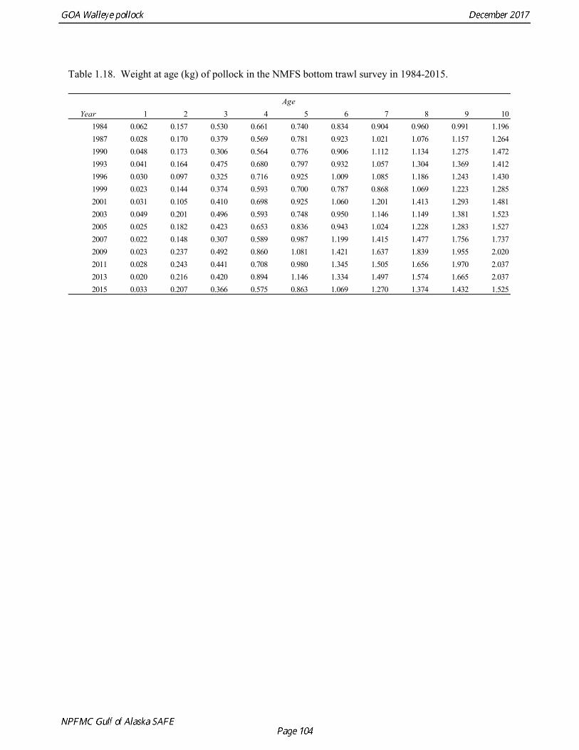
Table 1.18. Weight at age (kg) of pollock in the NMFS bottom trawl survey in 1984-2015.

AgeYear 1 2 3 4 5 6 7 8 9 10

1984 0.062 0.157 0.530 0.661 0.740 0.834 0.904 0.960 0.991 1.1961987 0.028 0.170 0.379 0.569 0.781 0.923 1.021 1.076 1.157 1.2641990 0.048 0.173 0.306 0.564 0.776 0.906 1.112 1.134 1.275 1.4721993 0.041 0.164 0.475 0.680 0.797 0.932 1.057 1.304 1.369 1.4121996 0.030 0.097 0.325 0.716 0.925 1.009 1.085 1.186 1.243 1.4301999 0.023 0.144 0.374 0.593 0.700 0.787 0.868 1.069 1.223 1.2852001 0.031 0.105 0.410 0.698 0.925 1.060 1.201 1.413 1.293 1.4812003 0.049 0.201 0.496 0.593 0.748 0.950 1.146 1.149 1.381 1.5232005 0.025 0.182 0.423 0.653 0.836 0.943 1.024 1.228 1.283 1.5272007 0.022 0.148 0.307 0.589 0.987 1.199 1.415 1.477 1.756 1.7372009 0.023 0.237 0.492 0.860 1.081 1.421 1.637 1.839 1.955 2.0202011 0.028 0.243 0.441 0.708 0.980 1.345 1.505 1.656 1.970 2.0372013 0.020 0.216 0.420 0.894 1.146 1.334 1.497 1.574 1.665 2.0372015 0.033 0.207 0.366 0.575 0.863 1.069 1.270 1.374 1.432 1.525

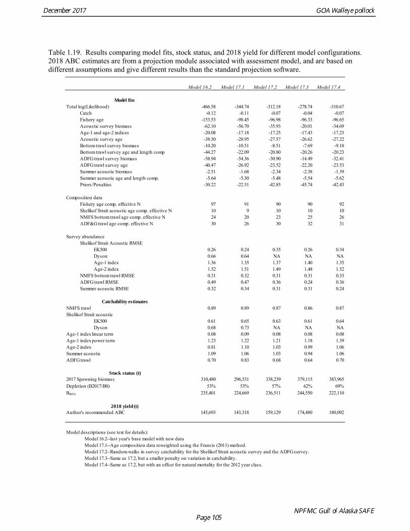
Table 1.19. Results comparing model fits, stock status, and 2018 yield for different model configurations. 2018 ABC estimates are from a projection module associated with assessment model, and are based on different assumptions and give different results than the standard projection software.

Model 16.2 Model 17.1 Model 17.2 Model 17.3 Model 17.4

Model fitsTotal log(Likelihood) -466.58 -344.74 -312.18 -278.74 -310.67

Catch -0.12 -0.11 -0.07 -0.04 -0.07Fishery age -153.53 -98.45 -96.98 -96.33 -96.65Acoustic survey biomass -62.10 -56.70 -35.93 -20.01 -34.69Age-1 and age-2 indices -20.08 -17.18 -17.25 -17.43 -17.23Acoustic survey age -38.50 -28.95 -27.57 -26.62 -27.22Bottom trawl survey biomass -10.20 -10.51 -8.51 -7.69 -9.18Bottom trawl survey age and length comp -44.27 -22.09 -20.80 -20.26 -20.23ADFG trawl survey biomass -58.94 -54.36 -30.90 -14.49 -32.41ADFG trawl survey age -40.47 -26.92 -23.52 -22.20 -23.53Summer acoustic biomass -2.51 -1.68 -2.34 -2.38 -1.39Summer acoustic age and length comp. -5.64 -5.30 -5.48 -5.54 -5.62Priors/Penalties -30.22 -22.51 -42.85 -45.74 -42.43

Composition dataFishery age comp. effective N 97 91 90 90 92Shelikof Strait acoustic age comp. effective N 10 9 10 10 10NMFS bottom trawl age comp. effective N 24 20 23 25 26ADF&G trawl age comp. effective N 30 26 30 32 31

Survey abundanceShelikof Strait Acoustic RMSE

EK500 0.26 0.24 0.35 0.26 0.34Dyson 0.66 0.64 NA NA NAAge-1 index 1.36 1.35 1.37 1.40 1.35Age-2 index 1.52 1.51 1.49 1.48 1.52

NMFS bottom trawl RMSE 0.31 0.32 0.31 0.31 0.33ADFG trawl RMSE 0.49 0.47 0.36 0.24 0.36Summer acoustic RMSE 0.32 0.34 0.31 0.31 0.24

Catchability estimatesNMFS trawl 0.89 0.89 0.87 0.86 0.87Shelikof Strait acoustic

EK500 0.61 0.65 0.63 0.61 0.64Dyson 0.68 0.73 NA NA NA

Age-1 index linear term 0.08 0.09 0.08 0.08 0.08Age-1 index power term 1.23 1.22 1.21 1.18 1.39Age-2 index 0.81 1.10 1.03 0.99 1.06Summer acoustic 1.09 1.06 1.03 0.94 1.06ADFG trawl 0.70 0.83 0.68 0.64 0.70

Stock status (t)2017 Spawning biomass 310,480 296,531 338,239 379,115 383,965Depletion (B2017/B0) 53% 53% 57% 62% 69%B40% 235,401 224,669 236,511 244,550 222,110

2018 yield (t)Author's recommended ABC 145,693 143,318 159,129 174,480 180,092

Model descriptions (see text for details):Model 16.2--last year's base model with new dataModel 17.1--Age composition data reweighted using the Francis (2011) method.Model 17.2--Random walks in survey catchability for the Shelikof Strait acoustic survey and the ADFG survey.Model 17.3--Same as 17.2, but a smaller penalty on variation in catchability.Model 17.4--Same as 17.2, but with an offset for natural mortality for the 2012 year class.

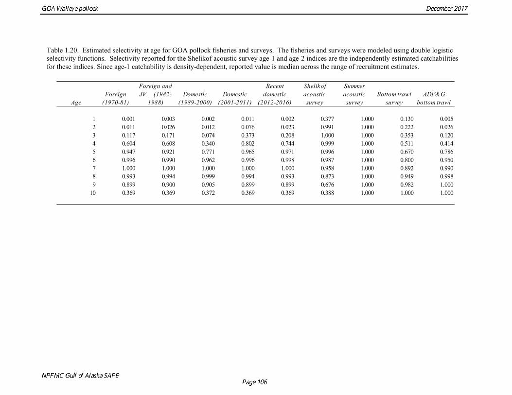
Table 1.20. Estimated selectivity at age for GOA pollock fisheries and surveys. The fisheries and surveys were modeled using double logistic selectivity functions. Selectivity reported for the Shelikof acoustic survey age-1 and age-2 indices are the independently estimated catchabilities for these indices. Since age-1 catchability is density-dependent, reported value is median across the range of recruitment estimates.

AgeForeign

(1970-81)

Foreign and JV (1982-

1988)Domestic

(1989-2000)Domestic

(2001-2011)

Recent domestic

(2012-2016)

Shelikof acoustic survey

Summer acoustic survey

Bottom trawl survey

ADF&G bottom trawl

1 0.001 0.003 0.002 0.011 0.002 0.377 1.000 0.130 0.0052 0.011 0.026 0.012 0.076 0.023 0.991 1.000 0.222 0.0263 0.117 0.171 0.074 0.373 0.208 1.000 1.000 0.353 0.1204 0.604 0.608 0.340 0.802 0.744 0.999 1.000 0.511 0.4145 0.947 0.921 0.771 0.965 0.971 0.996 1.000 0.670 0.7866 0.996 0.990 0.962 0.996 0.998 0.987 1.000 0.800 0.9507 1.000 1.000 1.000 1.000 1.000 0.958 1.000 0.892 0.9908 0.993 0.994 0.999 0.994 0.993 0.873 1.000 0.949 0.9989 0.899 0.900 0.905 0.899 0.899 0.676 1.000 0.982 1.000

10 0.369 0.369 0.372 0.369 0.369 0.388 1.000 1.000 1.000

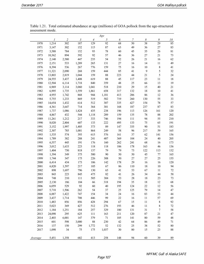
Table 1.21. Total estimated abundance at age (millions) of GOA pollock from the age-structured assessment mode.

Age1 2 3 4 5 6 7 8 9 10

1970 1,214 302 187 129 92 68 50 38 29 851971 3,147 302 152 115 87 63 49 36 27 831972 3,588 784 152 93 78 60 45 35 26 811973 10,362 894 392 92 57 46 36 27 21 731974 2,140 2,580 447 235 54 32 26 21 16 621975 2,151 533 1,289 265 131 27 16 14 11 491976 8,394 536 267 776 159 75 16 10 8 411977 11,321 2,090 268 159 444 85 41 9 5 321978 13,803 2,819 1,044 159 88 223 44 21 5 241979 24,555 3,437 1,408 619 88 45 117 23 11 181980 12,504 6,114 1,718 840 359 48 25 66 13 191981 6,969 3,114 3,060 1,041 518 210 29 15 40 211982 6,995 1,735 1,559 1,861 658 317 132 18 10 411983 4,955 1,742 868 944 1,181 413 206 86 12 361984 5,755 1,233 869 519 582 719 260 130 55 331985 14,654 1,432 614 512 307 335 427 154 78 571986 4,361 3,647 714 364 301 168 187 237 87 831987 1,737 1,086 1,824 435 238 196 113 126 161 1201988 4,867 432 544 1,118 289 159 135 78 88 2021989 11,261 1,212 217 333 746 194 111 94 55 2101990 8,020 2,804 607 133 222 495 133 75 65 1911991 3,152 1,997 1,405 373 89 147 335 90 51 1831992 2,307 785 1,001 864 249 58 96 217 59 1651993 1,535 574 393 615 576 161 37 62 141 1561994 1,789 382 288 241 407 369 104 24 40 2051995 6,557 445 191 176 160 262 241 68 16 1731996 3,012 1,633 223 118 118 106 178 163 46 1361997 1,404 750 818 137 79 79 73 122 113 1321998 1,394 349 375 500 90 50 50 45 77 1651999 1,744 347 175 226 308 50 27 27 25 1552000 6,414 434 173 106 142 178 29 16 16 1202001 6,820 1,597 217 105 67 86 110 18 10 942002 898 1,697 796 130 65 41 53 67 11 722003 843 223 845 475 82 41 26 34 44 582004 748 210 111 505 304 53 28 18 23 732005 2,130 186 104 66 318 194 35 18 12 682006 6,059 529 92 60 40 195 124 22 12 562007 5,718 1,506 262 54 37 25 125 79 14 472008 6,887 1,422 747 154 34 24 16 83 53 442009 3,437 1,714 708 446 99 22 16 11 57 692010 1,483 856 856 428 294 67 15 11 8 922011 5,023 369 427 512 276 193 46 11 8 722012 1,184 1,251 184 257 329 180 131 31 7 582013 24,098 295 625 111 163 211 120 87 21 472014 2,403 6,001 147 379 71 105 141 80 59 482015 601 598 3,000 88 230 42 64 86 49 712016 137 150 299 1,772 52 132 25 38 52 802017 1,098 34 75 175 1,037 30 80 15 23 88

Average 5,451 1,358 682 413 258 148 94 60 39 89

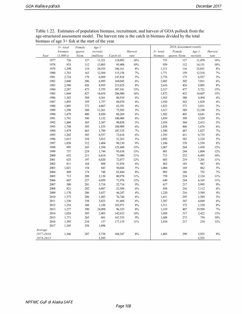
Table 1.22. Estimates of population biomass, recruitment, and harvest of GOA pollock from the age-structured assessment model. The harvest rate is the catch in biomass divided by the total biomass of age 3+ fish at the start of the year.

3+ total biomass

Female spawn. biom.

Age 1 recruits

Harvest rate

1977 726 127 11,321 118,092 16% 733 127 11,459 16%1978 933 112 13,803 95,408 10% 939 112 14,131 10%1979 1,298 119 24,555 106,161 8% 1,311 116 25,051 8%1980 1,743 163 12,504 115,158 7% 1,771 159 12,518 7%1981 2,724 179 6,969 147,818 5% 2,776 175 6,937 5%1982 2,840 306 6,995 169,045 6% 2,885 302 7,031 6%1983 2,580 426 4,955 215,625 8% 2,616 426 5,005 8%1984 2,287 473 5,755 307,541 13% 2,317 477 5,721 13%1985 1,844 427 14,654 286,900 16% 1,872 432 14,607 15%1986 1,543 384 4,361 86,910 6% 1,563 388 4,494 6%1987 1,895 359 1,737 68,070 4% 1,910 363 1,829 4%1988 1,805 372 4,867 63,391 4% 1,823 373 5,031 3%1989 1,598 388 11,261 75,585 5% 1,617 389 12,198 5%1990 1,479 400 8,020 88,269 6% 1,502 403 8,641 6%1991 1,791 396 3,152 100,488 6% 1,859 399 3,529 5%1992 1,860 365 2,307 90,858 5% 1,954 368 2,415 5%1993 1,748 395 1,535 108,909 6% 1,858 406 1,676 6%1994 1,479 463 1,789 107,335 7% 1,580 487 1,827 7%1995 1,202 385 6,557 72,618 6% 1,293 411 6,735 6%1996 1,013 354 3,012 51,263 5% 1,092 382 3,324 5%1997 1,038 312 1,404 90,130 9% 1,106 339 1,530 8%1998 995 243 1,394 125,460 13% 1,067 264 1,458 12%1999 737 224 1,744 95,638 13% 801 244 1,804 12%2000 652 211 6,414 73,080 11% 713 232 6,495 10%2001 625 197 6,820 72,077 12% 683 219 7,201 11%2002 811 164 898 51,934 6% 862 183 947 6%2003 1,021 154 843 50,684 5% 1,084 169 862 5%2004 849 174 748 63,844 8% 903 186 752 7%2005 713 209 2,130 80,978 11% 759 224 2,124 11%2006 607 227 6,059 71,976 12% 649 244 6,165 11%2007 580 201 5,718 52,714 9% 617 217 5,995 9%2008 821 202 6,887 52,584 6% 858 216 7,112 6%2009 1,170 206 3,437 44,247 4% 1,220 216 3,589 4%2010 1,375 286 1,483 76,744 6% 1,431 295 1,569 5%2011 1,330 338 5,023 81,484 6% 1,387 347 4,849 6%2012 1,254 360 1,184 103,971 8% 1,311 372 1,320 8%2013 1,277 390 24,098 96,353 8% 1,319 407 19,950 7%2014 1,024 305 2,403 142,632 14% 1,058 317 2,422 13%2015 1,771 265 601 167,553 9% 1,608 273 754 10%2016 1,595 234 137 177,135 11% 1,434 217 210 12%2017 1,345 258 1,098

Average1977-2016 1,366 287 5,738 104,347 8% 1,403 299 5,925 8%1978-2015 5,595 5,553

Year

2016 Assessment results3+ total biomass (1,000 t)

Female spawn. biom.

Age 1 recruits

(million) Catch (t)Harvest

rate

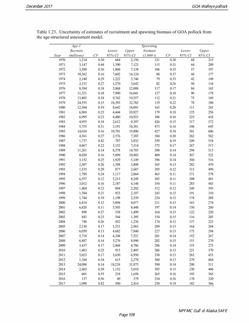
Table 1.23. Uncertainty of estimates of recruitment and spawning biomass of GOA pollock from the age-structured assessment model.

Year

Age-1 Recruits

(millions) CVLower

95% CIUpper

95% CI

Spawning biomass (1,000 t) CV

Lower 95% CI

Upper 95% CI

1970 1,214 0.30 684 2,156 121 0.30 68 2151971 3,147 0.44 1,390 7,123 115 0.31 64 2091972 3,588 0.36 1,804 7,138 106 0.33 57 1971973 10,362 0.16 7,602 14,124 88 0.37 44 1771974 2,140 0.29 1,222 3,746 79 0.33 42 1491975 2,151 0.27 1,270 3,642 82 0.26 50 1341976 8,394 0.18 5,868 12,008 117 0.17 84 1631977 11,321 0.18 7,990 16,041 127 0.18 90 1781978 13,803 0.18 9,742 19,557 112 0.21 75 1691979 24,555 0.15 18,393 32,782 119 0.22 78 1801980 12,504 0.19 8,642 18,091 163 0.20 111 2411981 6,969 0.23 4,444 10,927 179 0.18 125 2561982 6,995 0.23 4,480 10,923 306 0.16 225 4181983 4,955 0.34 2,612 9,397 426 0.15 317 5721984 5,755 0.31 3,191 10,381 473 0.16 346 6451985 14,654 0.16 10,791 19,900 427 0.18 301 6061986 4,361 0.27 2,576 7,385 384 0.20 262 5621987 1,737 0.42 787 3,832 359 0.19 249 5181988 4,867 0.22 3,152 7,514 372 0.17 267 5171989 11,261 0.14 8,578 14,783 388 0.14 294 5131990 8,020 0.16 5,899 10,903 400 0.14 307 5221991 3,152 0.25 1,929 5,149 396 0.14 304 5161992 2,307 0.26 1,398 3,808 365 0.13 282 4701993 1,535 0.29 877 2,687 395 0.12 313 4991994 1,789 0.24 1,117 2,864 463 0.11 371 5781995 6,557 0.12 5,213 8,249 385 0.11 308 4811996 3,012 0.16 2,187 4,148 354 0.11 283 4431997 1,404 0.23 894 2,202 312 0.12 249 3931998 1,394 0.21 923 2,107 243 0.12 191 3101999 1,744 0.19 1,198 2,539 224 0.13 174 2882000 6,414 0.12 5,094 8,077 211 0.13 163 2742001 6,820 0.11 5,505 8,448 197 0.14 150 2602002 898 0.27 538 1,499 164 0.15 122 2202003 843 0.23 544 1,305 154 0.15 116 2052004 748 0.26 452 1,236 174 0.13 137 2232005 2,130 0.17 1,531 2,963 209 0.13 164 2682006 6,059 0.13 4,682 7,840 227 0.13 175 2942007 5,718 0.14 4,348 7,521 201 0.14 152 2672008 6,887 0.14 5,276 8,990 202 0.15 151 2702009 3,437 0.17 2,468 4,786 206 0.14 155 2732010 1,483 0.25 915 2,405 286 0.13 221 3702011 5,023 0.17 3,630 6,950 338 0.13 263 4332012 1,184 0.34 615 2,278 360 0.13 279 4642013 24,098 0.14 18,218 31,875 390 0.14 298 5112014 2,403 0.39 1,152 5,010 305 0.15 230 4062015 601 0.55 218 1,658 265 0.16 193 3652016 137 0.56 49 379 234 0.16 170 3202017 1,098 0.42 500 2,414 258 0.18 182 366

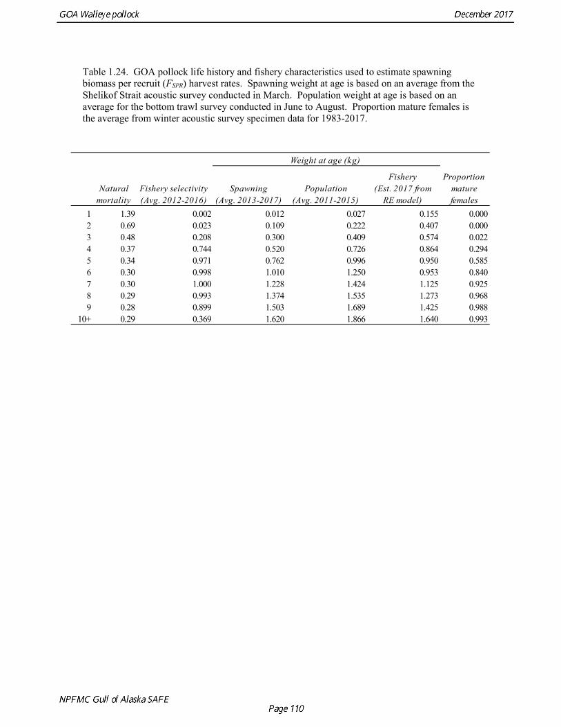
Table 1.24. GOA pollock life history and fishery characteristics used to estimate spawning biomass per recruit (FSPR) harvest rates. Spawning weight at age is based on an average from the Shelikof Strait acoustic survey conducted in March. Population weight at age is based on an average for the bottom trawl survey conducted in June to August. Proportion mature females is the average from winter acoustic survey specimen data for 1983-2017.

Spawning (Avg. 2013-2017)

Population (Avg. 2011-2015)

Fishery (Est. 2017 from

RE model)1 1.39 0.002 0.012 0.027 0.155 0.0002 0.69 0.023 0.109 0.222 0.407 0.0003 0.48 0.208 0.300 0.409 0.574 0.0224 0.37 0.744 0.520 0.726 0.864 0.2945 0.34 0.971 0.762 0.996 0.950 0.5856 0.30 0.998 1.010 1.250 0.953 0.8407 0.30 1.000 1.228 1.424 1.125 0.9258 0.29 0.993 1.374 1.535 1.273 0.9689 0.28 0.899 1.503 1.689 1.425 0.988

10+ 0.29 0.369 1.620 1.866 1.640 0.993

Proportion mature females

Natural mortality

Fishery selectivity (Avg. 2012-2016)

Weight at age (kg)

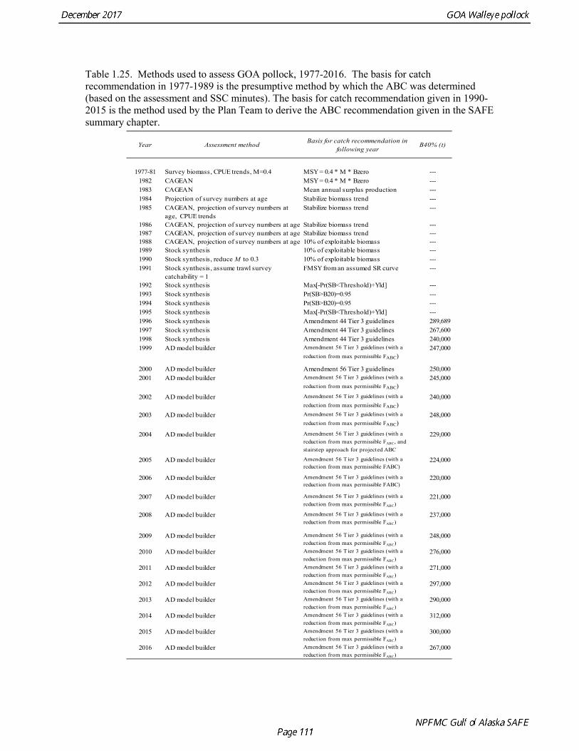
Table 1.25. Methods used to assess GOA pollock, 1977-2016. The basis for catch recommendation in 1977-1989 is the presumptive method by which the ABC was determined (based on the assessment and SSC minutes). The basis for catch recommendation given in 1990-2015 is the method used by the Plan Team to derive the ABC recommendation given in the SAFE summary chapter.

Year Assessment method Basis for catch recommendation in following year

B40% (t)

1977-81 Survey biomass, CPUE trends, M=0.4 MSY = 0.4 * M * Bzero ---1982 CAGEAN MSY = 0.4 * M * Bzero ---1983 CAGEAN Mean annual surplus production ---1984 Projection of survey numbers at age Stabilize biomass trend ---1985 CAGEAN, projection of survey numbers at

age, CPUE trendsStabilize biomass trend ---

1986 CAGEAN, projection of survey numbers at age Stabilize biomass trend ---1987 CAGEAN, projection of survey numbers at age Stabilize biomass trend ---1988 CAGEAN, projection of survey numbers at age 10% of exploitable biomass ---1989 Stock synthesis 10% of exploitable biomass ---1990 Stock synthesis, reduce M to 0.3 10% of exploitable biomass ---1991 Stock synthesis, assume trawl survey

catchability = 1FMSY from an assumed SR curve ---

1992 Stock synthesis Max[-Pr(SB<Threshold)+Yld] ---1993 Stock synthesis Pr(SB>B20)=0.95 ---1994 Stock synthesis Pr(SB>B20)=0.95 ---1995 Stock synthesis Max[-Pr(SB<Threshold)+Yld] ---1996 Stock synthesis Amendment 44 Tier 3 guidelines 289,6891997 Stock synthesis Amendment 44 Tier 3 guidelines 267,6001998 Stock synthesis Amendment 44 Tier 3 guidelines 240,0001999 AD model builder Amendment 56 T ier 3 guidelines (with a

reduction from max permissible FABC)247,000

2000 AD model builder Amendment 56 Tier 3 guidelines 250,0002001 AD model builder Amendment 56 T ier 3 guidelines (with a

reduction from max permissible FABC)245,000

2002 AD model builder Amendment 56 T ier 3 guidelines (with a reduction from max permissible FABC)

240,000

2003 AD model builder Amendment 56 T ier 3 guidelines (with a reduction from max permissible FABC)

248,000

2004 AD model builder Amendment 56 T ier 3 guidelines (with a reduction from max permissible FABC, and stairstep approach for projected ABC

229,000

2005 AD model builder Amendment 56 T ier 3 guidelines (with a reduction from max permissible FABC)

224,000

2006 AD model builder Amendment 56 T ier 3 guidelines (with a reduction from max permissible FABC)

220,000

2007 AD model builder Amendment 56 T ier 3 guidelines (with a reduction from max permissible FABC)

221,000

2008 AD model builder Amendment 56 T ier 3 guidelines (with a reduction from max permissible FABC)

237,000

2009 AD model builder Amendment 56 T ier 3 guidelines (with a reduction from max permissible FABC)

248,000

2010 AD model builder Amendment 56 T ier 3 guidelines (with a reduction from max permissible FABC)

276,000

2011 AD model builder Amendment 56 T ier 3 guidelines (with a reduction from max permissible FABC)

271,000

2012 AD model builder Amendment 56 T ier 3 guidelines (with a reduction from max permissible FABC)

297,000

2013 AD model builder Amendment 56 T ier 3 guidelines (with a reduction from max permissible FABC)

290,000

2014 AD model builder Amendment 56 T ier 3 guidelines (with a reduction from max permissible FABC)

312,000

2015 AD model builder Amendment 56 T ier 3 guidelines (with a reduction from max permissible FABC)

300,000

2016 AD model builder Amendment 56 T ier 3 guidelines (with a reduction from max permissible FABC)

267,000

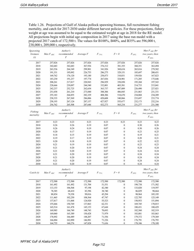
Table 1.26. Projections of Gulf of Alaska pollock spawning biomass, full recruitment fishing mortality, and catch for 2017-2030 under different harvest policies. For these projections, fishery weight at age was assumed to be equal to the estimated weight at age in 2018 for the RE model. All projections begin with initial age composition in 2017 using the base run model with a projected 2017 catch of 172,500 t. The values for B100%, B40%, and B35% are 596,000 t, 238,000 t, 209,000 t, respectively.

Spawning biomass

(t)Max F ABC

Author's recommended

FAverage F F 75% F = 0 F OFL

Max F ABC for two years, then

F OFL

2017 257,826 257,826 257,826 257,826 257,826 257,826 257,8262018 342,683 342,683 367,936 376,312 381,355 360,351 363,4942019 263,536 264,349 299,901 341,926 369,634 265,816 279,5022020 191,331 195,092 226,753 286,275 329,151 185,697 200,4312021 169,762 176,120 193,180 258,873 310,031 159,926 167,8232022 183,230 191,237 197,774 267,836 324,901 171,285 175,6462023 208,261 217,817 220,943 296,929 358,850 195,268 197,5432024 228,666 239,097 244,540 332,001 403,581 214,733 215,8412025 242,237 252,725 262,654 363,737 447,889 226,490 227,0212026 251,038 261,210 273,840 388,306 486,045 231,063 231,3312027 255,183 264,855 282,329 408,306 518,670 234,068 234,2092028 258,335 267,569 286,006 420,608 540,866 233,697 233,7742029 258,193 267,124 287,157 427,927 555,677 232,173 232,2162030 256,762 265,508 287,646 432,273 565,234 231,277 231,300

Fishing mortality

Max F ABC

Author's recommended

FAverage F F 75% F = 0 F OFL

Max F ABC for two years, then

F OFL

2017 0.23 0.23 0.23 0.23 0.23 0.23 0.232018 0.26 0.26 0.19 0.07 0 0.30 0.262019 0.26 0.24 0.19 0.07 0 0.30 0.262020 0.20 0.17 0.19 0.07 0 0.23 0.252021 0.18 0.15 0.19 0.07 0 0.19 0.212022 0.19 0.17 0.19 0.07 0 0.20 0.212023 0.20 0.18 0.19 0.07 0 0.22 0.222024 0.21 0.19 0.19 0.07 0 0.23 0.232025 0.21 0.20 0.19 0.07 0 0.24 0.242026 0.21 0.20 0.19 0.07 0 0.24 0.242027 0.21 0.20 0.19 0.07 0 0.24 0.242028 0.21 0.20 0.19 0.07 0 0.24 0.242029 0.21 0.20 0.19 0.07 0 0.24 0.242030 0.21 0.20 0.19 0.07 0 0.24 0.24

Catch (t) Max F ABC

Author's recommended

FAverage F F 75% F = 0 F OFL

Max F ABC for two years, then

F OFL

2017 172,500 172,500 172,500 172,500 172,500 172,500 172,5002018 161,492 161,492 131,704 51,551 0 198,738 171,5822019 113,153 106,568 97,198 42,340 0 133,020 119,5972020 78,385 68,410 83,596 38,740 0 86,029 98,6642021 88,854 79,358 99,016 45,294 0 98,964 105,1952022 111,465 102,250 108,564 47,747 0 122,785 125,1492023 137,817 131,068 124,920 55,523 0 150,953 151,8942024 155,666 150,769 137,063 62,331 0 169,745 170,0152025 165,514 161,478 145,153 67,644 0 180,431 180,4292026 169,985 166,749 148,743 70,693 0 182,560 182,5192027 169,060 165,389 150,428 71,979 0 183,881 183,8632028 170,492 166,489 148,207 71,556 0 179,372 179,3692029 166,884 162,890 146,981 71,226 0 176,791 176,7932030 164,755 160,276 147,828 71,636 0 178,106 178,109

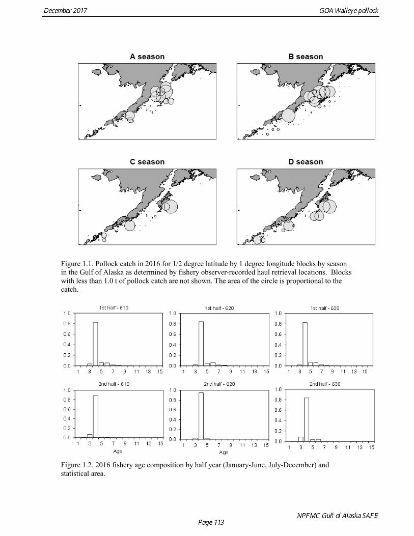
Figure 1.1. Pollock catch in 2016 for 1/2 degree latitude by 1 degree longitude blocks by season in the Gulf of Alaska as determined by fishery observer-recorded haul retrieval locations. Blocks with less than 1.0 t of pollock catch are not shown. The area of the circle is proportional to the catch.

Figure 1.2. 2016 fishery age composition by half year (January-June, July-December) and statistical area.

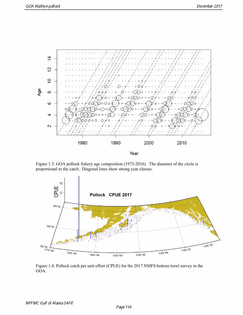
Figure 1.3. GOA pollock fishery age composition (1975-2016). The diameter of the circle is proportional to the catch. Diagonal lines show strong year classes.

Figure 1.4. Pollock catch per unit effort (CPUE) for the 2017 NMFS bottom trawl survey in the GOA.

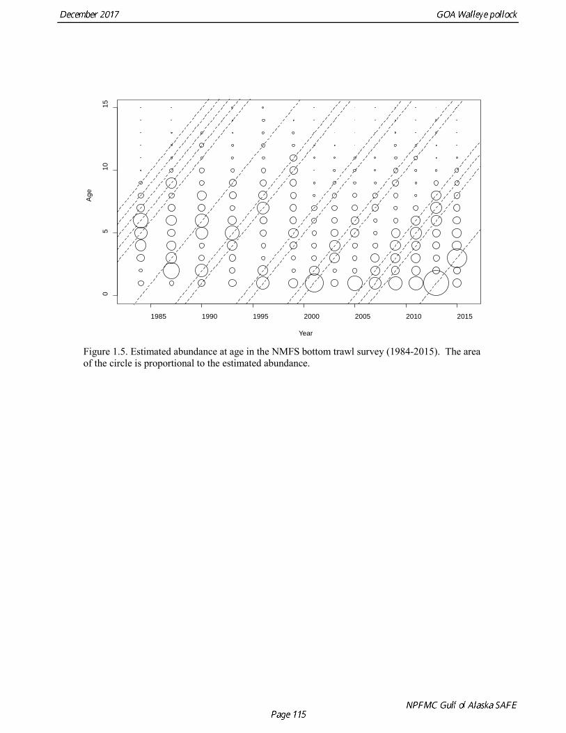
Figure 1.5. Estimated abundance at age in the NMFS bottom trawl survey (1984-2015). The area of the circle is proportional to the estimated abundance.

1985 1990 1995 2000 2005 2010 2015

05

1015

Year

Age

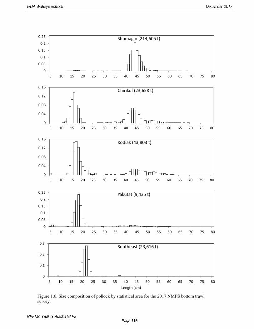
Figure 1.6. Size composition of pollock by statistical area for the 2017 NMFS bottom trawl survey.

0

0.05

0.1

0.15

0.2

0.25

5 10 15 20 25 30 35 40 45 50 55 60 65 70 75 80

Shumagin (214,605 t)

0

0.04

0.08

0.12

0.16

5 10 15 20 25 30 35 40 45 50 55 60 65 70 75 80

Chirikof (23,658 t)

0

0.04

0.08

0.12

0.16

5 10 15 20 25 30 35 40 45 50 55 60 65 70 75 80

Kodiak (43,803 t)

0

0.05

0.1

0.15

0.2

0.25

5 10 15 20 25 30 35 40 45 50 55 60 65 70 75 80

Yakutat (9,435 t)

0

0.1

0.2

0.3

5 10 15 20 25 30 35 40 45 50 55 60 65 70 75 80Length (cm)

Southeast (23,616 t)

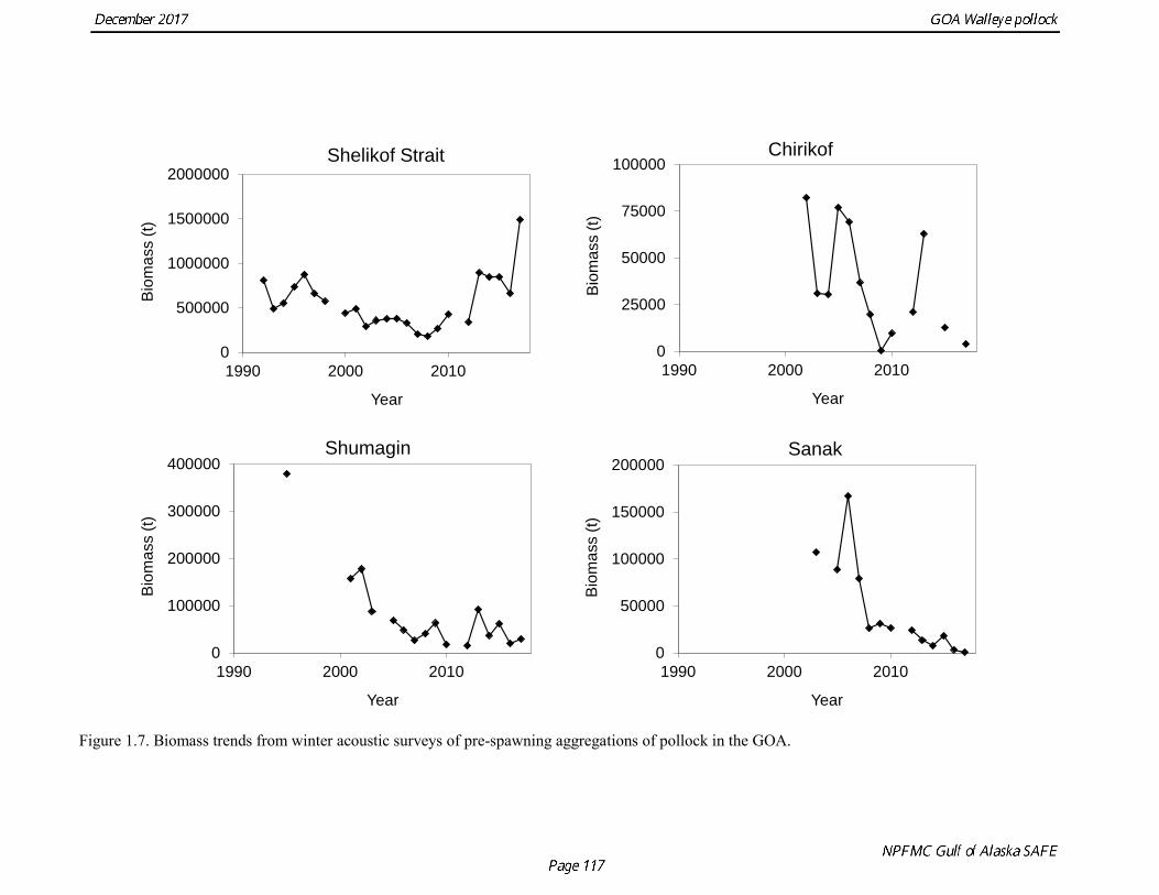
Figure 1.7. Biomass trends from winter acoustic surveys of pre-spawning aggregations of pollock in the GOA.

0

25000

50000

75000

100000

1990 2000 2010

Bio

mas

s (t)

Year

Chirikof

0

500000

1000000

1500000

2000000

1990 2000 2010

Bio

mas

s (t)

Year

Shelikof Strait

0

100000

200000

300000

400000

1990 2000 2010

Bio

mas

s (t)

Year

Shumagin

0

50000

100000

150000

200000

1990 2000 2010

Bio

mas

s (t)

Year

Sanak

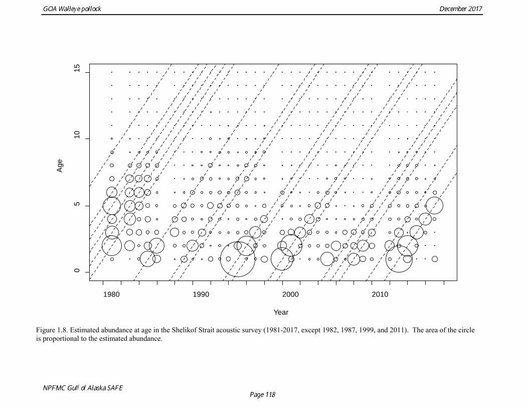
Figure 1.8. Estimated abundance at age in the Shelikof Strait acoustic survey (1981-2017, except 1982, 1987, 1999, and 2011). The area of the circle is proportional to the estimated abundance.

1980 1990 2000 2010

05

1015

Year

Age

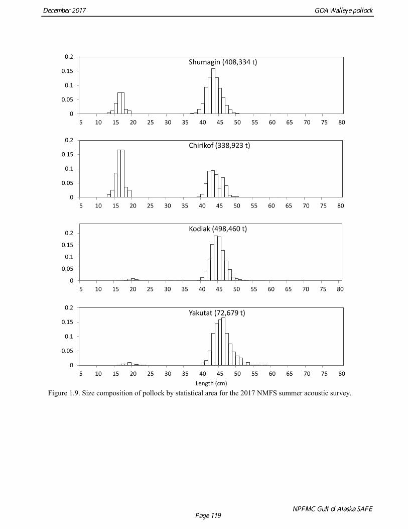
Figure 1.9. Size composition of pollock by statistical area for the 2017 NMFS summer acoustic survey.

0

0.05

0.1

0.15

0.2

5 10 15 20 25 30 35 40 45 50 55 60 65 70 75 80

Shumagin (408,334 t)

0

0.05

0.1

0.15

0.2

5 10 15 20 25 30 35 40 45 50 55 60 65 70 75 80

Chirikof (338,923 t)

0

0.05

0.1

0.15

0.2

5 10 15 20 25 30 35 40 45 50 55 60 65 70 75 80

Kodiak (498,460 t)

0

0.05

0.1

0.15

0.2

5 10 15 20 25 30 35 40 45 50 55 60 65 70 75 80Length (cm)

Yakutat (72,679 t)

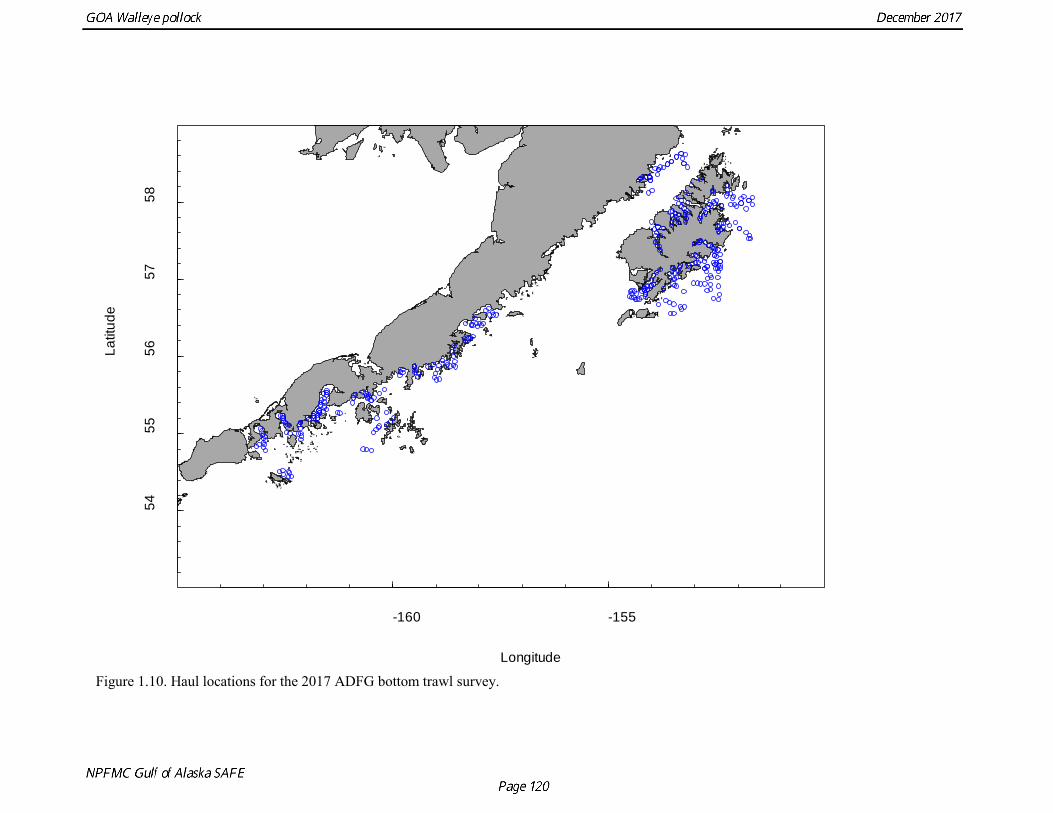
Figure 1.10. Haul locations for the 2017 ADFG bottom trawl survey.

-160 -155

5455

5657

58

Longitude

Latit

ude

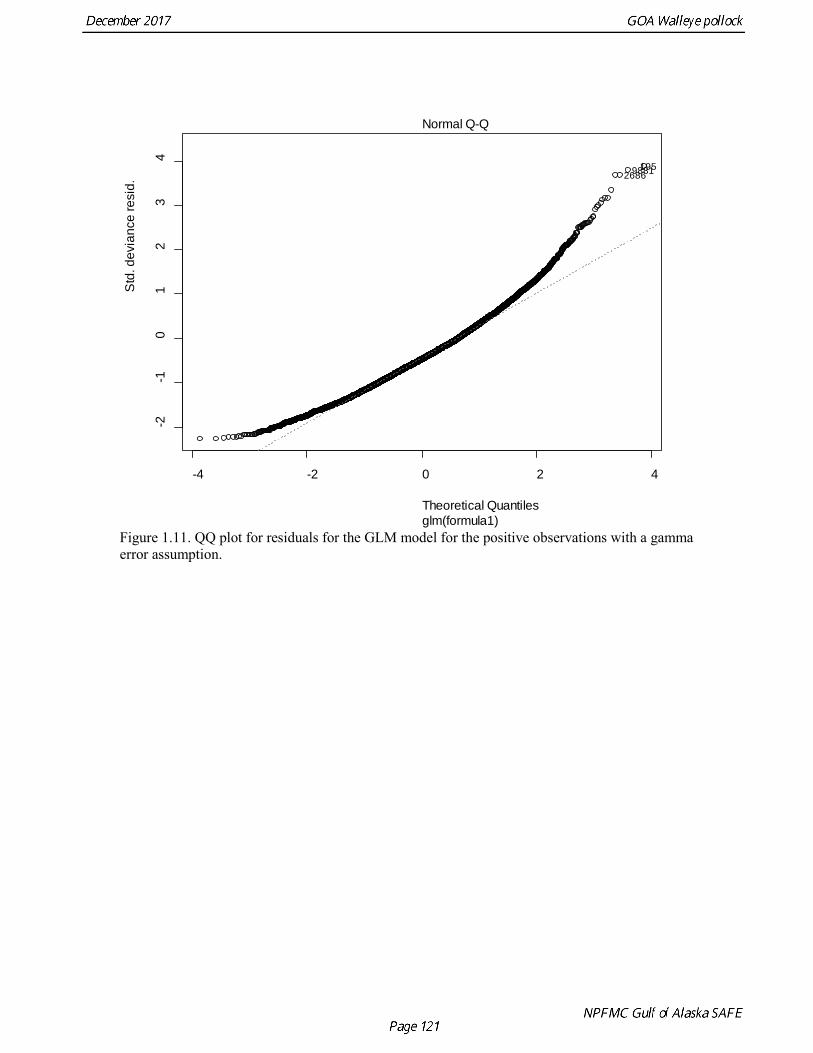
Figure 1.11. QQ plot for residuals for the GLM model for the positive observations with a gamma error assumption.

-4 -2 0 2 4

-2-1

01

23

4

Theoretical Quantiles

Std

. dev

ianc

e re

sid.

glm(formula1)

Normal Q-Q

19598812686

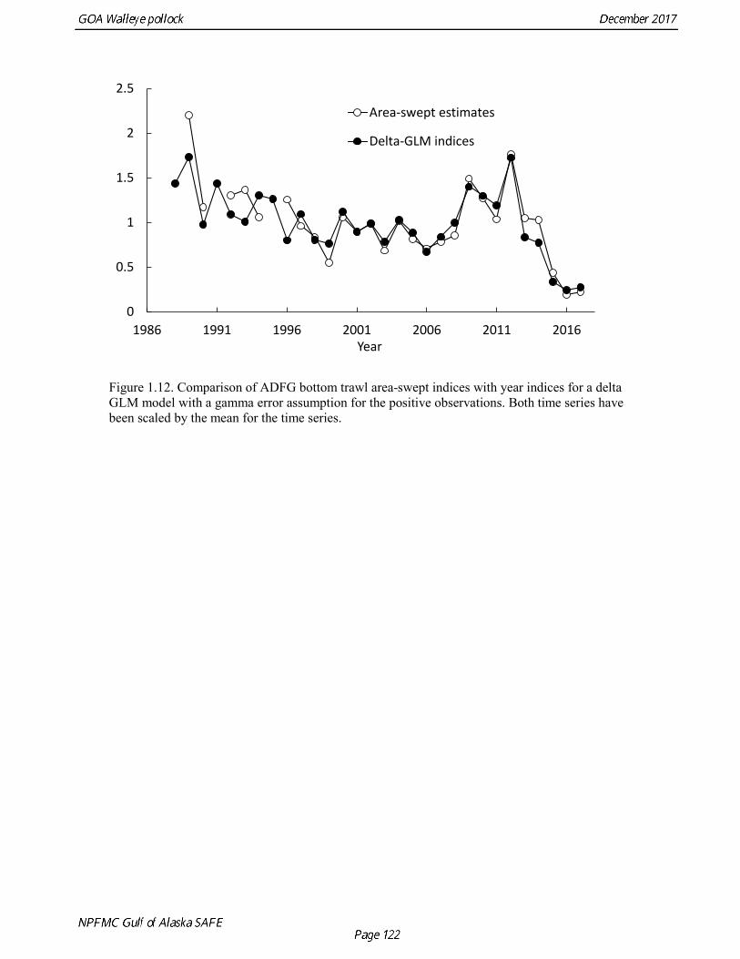
Figure 1.12. Comparison of ADFG bottom trawl area-swept indices with year indices for a delta GLM model with a gamma error assumption for the positive observations. Both time series have been scaled by the mean for the time series.

0

0.5

1

1.5

2

2.5

1986 1991 1996 2001 2006 2011 2016Year

Area-swept estimates

Delta-GLM indices

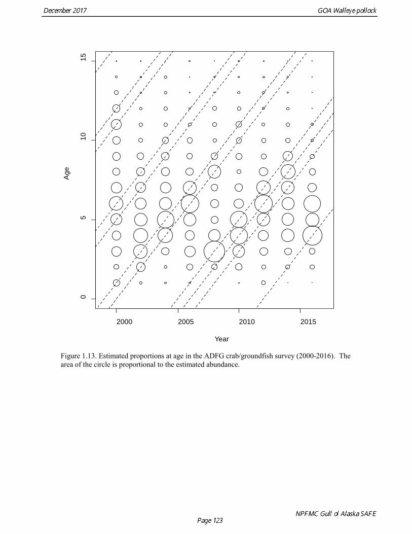
Figure 1.13. Estimated proportions at age in the ADFG crab/groundfish survey (2000-2016). The area of the circle is proportional to the estimated abundance.

2000 2005 2010 2015

05

1015

Year

Age

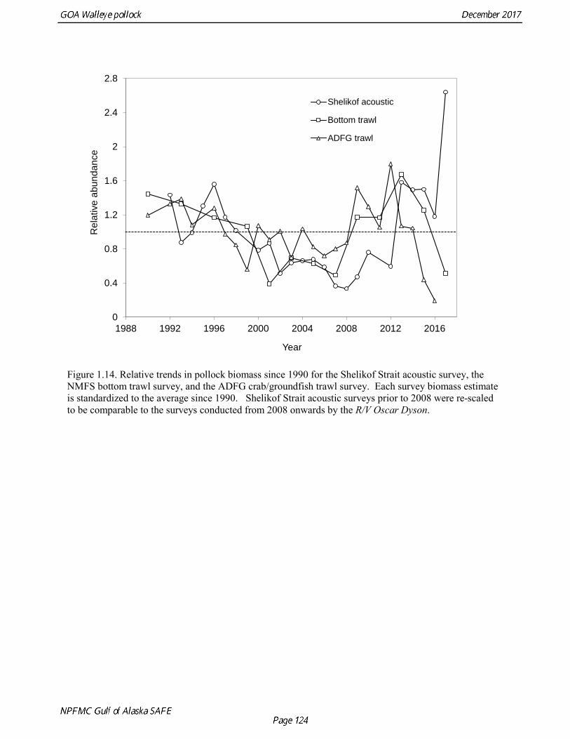
Figure 1.14. Relative trends in pollock biomass since 1990 for the Shelikof Strait acoustic survey, the NMFS bottom trawl survey, and the ADFG crab/groundfish trawl survey. Each survey biomass estimate is standardized to the average since 1990. Shelikof Strait acoustic surveys prior to 2008 were re-scaled to be comparable to the surveys conducted from 2008 onwards by the R/V Oscar Dyson.

0

0.4

0.8

1.2

1.6

2

2.4

2.8

1988 1992 1996 2000 2004 2008 2012 2016

Rel

ativ

e ab

unda

nce

Year

Shelikof acoustic

Bottom trawl

ADFG trawl

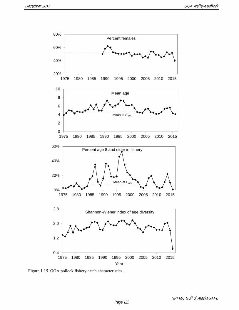
Figure 1.15. GOA pollock fishery catch characteristics.

20%

40%

60%

80%

1975 1980 1985 1990 1995 2000 2005 2010 2015

Percent females

0

2

4

6

8

10

1975 1980 1985 1990 1995 2000 2005 2010 2015

Mean age

Mean at F40%

0%

20%

40%

60%

1975 1980 1985 1990 1995 2000 2005 2010 2015

Percent age 8 and older in fishery

Mean at F40%

0.4

1.2

2.0

2.8

1975 1980 1985 1990 1995 2000 2005 2010 2015Year

Shannon-Wiener index of age diversity

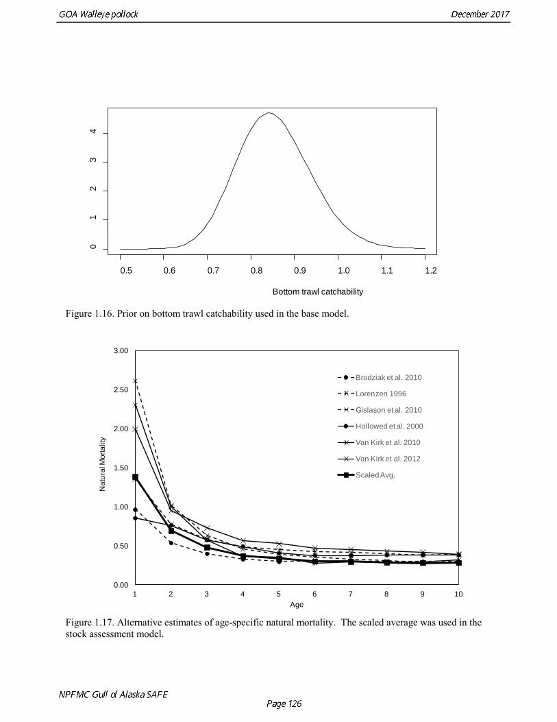
Figure 1.16. Prior on bottom trawl catchability used in the base model.

Figure 1.17. Alternative estimates of age-specific natural mortality. The scaled average was used in the stock assessment model.

0.5 0.6 0.7 0.8 0.9 1.0 1.1 1.2

01

23

4

Bottom trawl catchability

0.00

0.50

1.00

1.50

2.00

2.50

3.00

1 2 3 4 5 6 7 8 9 10

Nat

ural

Mor

talit

y

Age

Brodziak et al. 2010

Lorenzen 1996

Gislason et al. 2010

Hollowed et al. 2000

Van Kirk et al. 2010

Van Kirk et al. 2012

Scaled Avg.

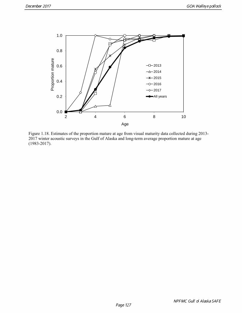
Figure 1.18. Estimates of the proportion mature at age from visual maturity data collected during 2013-2017 winter acoustic surveys in the Gulf of Alaska and long-term average proportion mature at age (1983-2017).

0.0

0.2

0.4

0.6

0.8

1.0

2 4 6 8 10

Pro

porti

on m

atur

e

Age

2013

2014

2015

2016

2017

All years

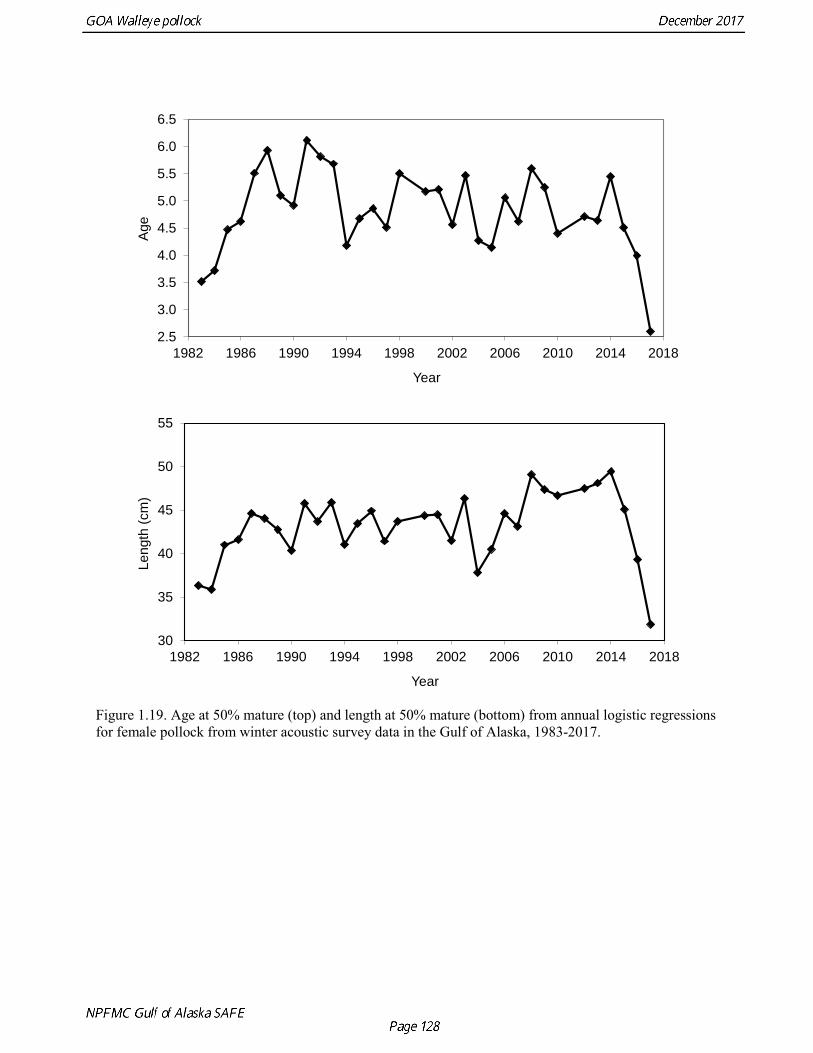
Figure 1.19. Age at 50% mature (top) and length at 50% mature (bottom) from annual logistic regressions for female pollock from winter acoustic survey data in the Gulf of Alaska, 1983-2017.

2.5

3.0

3.5

4.0

4.5

5.0

5.5

6.0

6.5

1982 1986 1990 1994 1998 2002 2006 2010 2014 2018

Age

Year

30

35

40

45

50

55

1982 1986 1990 1994 1998 2002 2006 2010 2014 2018

Leng

th (c

m)

Year

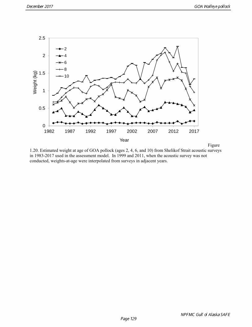
Figure 1.20. Estimated weight at age of GOA pollock (ages 2, 4, 6, and 10) from Shelikof Strait acoustic surveys in 1983-2017 used in the assessment model. In 1999 and 2011, when the acoustic survey was not conducted, weights-at-age were interpolated from surveys in adjacent years.

0

0.5

1

1.5

2

2.5

1982 1987 1992 1997 2002 2007 2012 2017

Wei

ght (

kg)

Year

246810

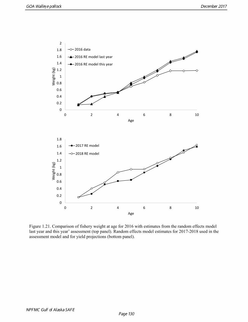
Figure 1.21. Comparison of fishery weight at age for 2016 with estimates from the random effects model last year and this year’ assessment (top panel). Random effects model estimates for 2017-2018 used in the assessment model and for yield projections (bottom panel).

0

0.2

0.4

0.6

0.8

1

1.2

1.4

1.6

1.8

2

0 2 4 6 8 10

Wei

ght (

kg)

Age

2016 data

2016 RE model last year

2016 RE model this year

0

0.2

0.4

0.6

0.8

1

1.2

1.4

1.6

1.8

0 2 4 6 8 10

Wei

ght (

kg)

Age

2017 RE model

2018 RE model

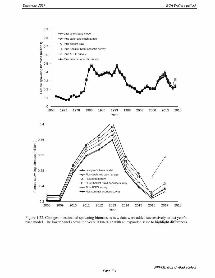
Figure 1.22. Changes in estimated spawning biomass as new data were added successively to last year’s base model. The lower panel shows the years 2008-2017 with an expanded scale to highlight differences.

0

0.1

0.2

0.3

0.4

0.5

0.6

0.7

0.8

0.9

1968 1973 1978 1983 1988 1993 1998 2003 2008 2013 2018

Fem

ale

spaw

ning

bio

mas

s (m

illion

t)

Year

Last year's base model

Plus catch and catch at age

Plus bottom trawl

Plus Shelikof Strait acoustic survey

Plus ADFG survey

Plus summer acoustic survey

0.2

0.24

0.28

0.32

0.36

0.4

2008 2009 2010 2011 2012 2013 2014 2015 2016 2017 2018

Fem

ale

spaw

ning

bio

mas

s (m

illion

t)

Year

Last year's base modelPlus catch and catch at agePlus bottom trawlPlus Shelikof Strait acoustic surveyPlus ADFG surveyPlus summer acoustic survey

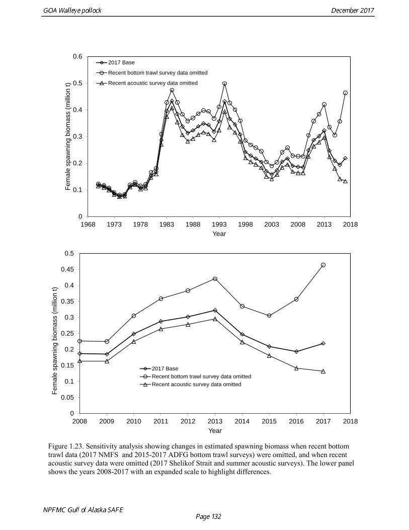
Figure 1.23. Sensitivity analysis showing changes in estimated spawning biomass when recent bottom trawl data (2017 NMFS and 2015-2017 ADFG bottom trawl surveys) were omitted, and when recent acoustic survey data were omitted (2017 Shelikof Strait and summer acoustic surveys). The lower panel shows the years 2008-2017 with an expanded scale to highlight differences.

0

0.1

0.2

0.3

0.4

0.5

0.6

1968 1973 1978 1983 1988 1993 1998 2003 2008 2013 2018

Fem

ale

spaw

ning

bio

mas

s (m

illion

t)

Year

2017 Base

Recent bottom trawl survey data omitted

Recent acoustic survey data omitted

0

0.05

0.1

0.15

0.2

0.25

0.3

0.35

0.4

0.45

0.5

2008 2009 2010 2011 2012 2013 2014 2015 2016 2017 2018

Fem

ale

spaw

ning

bio

mas

s (m

illion

t)

Year

2017 BaseRecent bottom trawl survey data omittedRecent acoustic survey data omitted

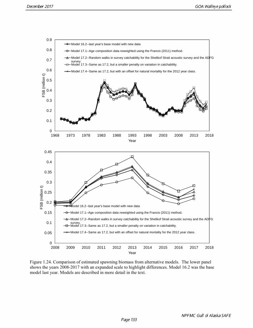
Figure 1.24. Comparison of estimated spawning biomass from alternative models. The lower panel shows the years 2008-2017 with an expanded scale to highlight differences. Model 16.2 was the base model last year. Models are described in more detail in the text.

0

0.1

0.2

0.3

0.4

0.5

0.6

0.7

0.8

0.9

1968 1973 1978 1983 1988 1993 1998 2003 2008 2013 2018

FSB

(milli

on t)

Year

Model 16.2--last year's base model with new data

Model 17.1--Age composition data reweighted using the Francis (2011) method.

Model 17.2--Random walks in survey catchability for the Shelikof Strait acoustic survey and the ADFGsurvey.Model 17.3--Same as 17.2, but a smaller penalty on variation in catchability.

Model 17.4--Same as 17.2, but with an offset for natural mortality for the 2012 year class.

0

0.05

0.1

0.15

0.2

0.25

0.3

0.35

0.4

0.45

2008 2009 2010 2011 2012 2013 2014 2015 2016 2017 2018

FSB

(milli

on t)

Year

Model 16.2--last year's base model with new data

Model 17.1--Age composition data reweighted using the Francis (2011) method.

Model 17.2--Random walks in survey catchability for the Shelikof Strait acoustic survey and the ADFGsurvey.Model 17.3--Same as 17.2, but a smaller penalty on variation in catchability.

Model 17.4--Same as 17.2, but with an offset for natural mortality for the 2012 year class.

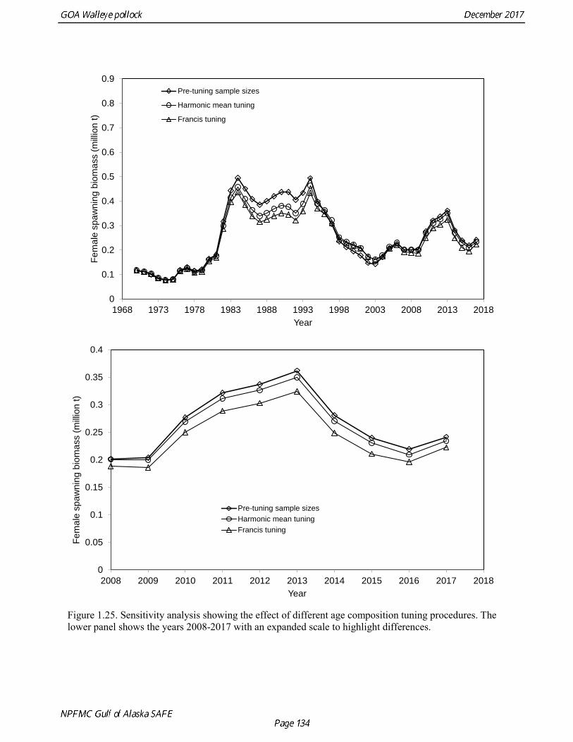
Figure 1.25. Sensitivity analysis showing the effect of different age composition tuning procedures. The lower panel shows the years 2008-2017 with an expanded scale to highlight differences.

0

0.1

0.2

0.3

0.4

0.5

0.6

0.7

0.8

0.9

1968 1973 1978 1983 1988 1993 1998 2003 2008 2013 2018

Fem

ale

spaw

ning

bio

mas

s (m

illion

t)

Year

Pre-tuning sample sizes

Harmonic mean tuning

Francis tuning

0

0.05

0.1

0.15

0.2

0.25

0.3

0.35

0.4

2008 2009 2010 2011 2012 2013 2014 2015 2016 2017 2018

Fem

ale

spaw

ning

bio

mas

s (m

illion

t)

Year

Pre-tuning sample sizesHarmonic mean tuningFrancis tuning

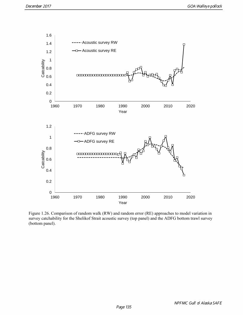
Figure 1.26. Comparison of random walk (RW) and random error (RE) approaches to model variation in survey catchability for the Shelikof Strait acoustic survey (top panel) and the ADFG bottom trawl survey (bottom panel).

0

0.2

0.4

0.6

0.8

1

1.2

1.4

1.6

1960 1970 1980 1990 2000 2010 2020

Cat

cabi

lity

Year

Acoustic survey RW

Acoustic survey RE

0

0.2

0.4

0.6

0.8

1

1.2

1960 1970 1980 1990 2000 2010 2020

Cat

cabi

lity

Year

ADFG survey RW

ADFG survey RE

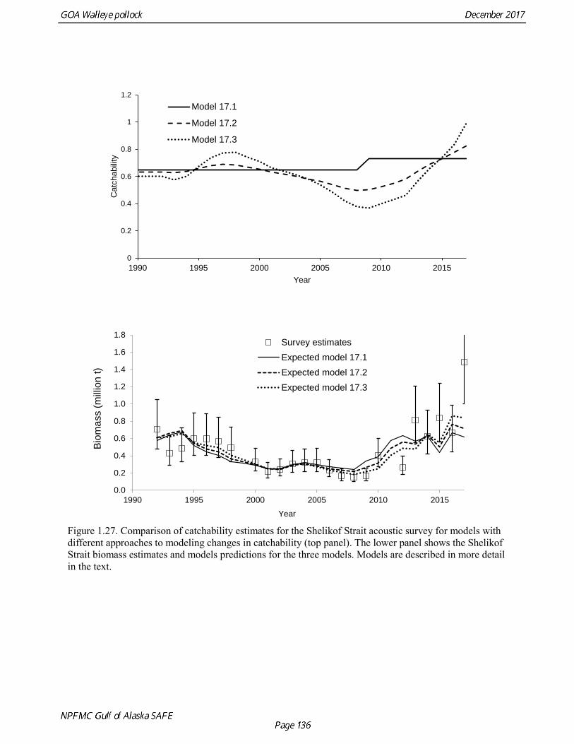
Figure 1.27. Comparison of catchability estimates for the Shelikof Strait acoustic survey for models with different approaches to modeling changes in catchability (top panel). The lower panel shows the Shelikof Strait biomass estimates and models predictions for the three models. Models are described in more detail in the text.

0.0

0.2

0.4

0.6

0.8

1.0

1.2

1.4

1.6

1.8

1990 1995 2000 2005 2010 2015

Bio

mas

s (m

illion

t)

Year

Survey estimatesExpected model 17.1Expected model 17.2Expected model 17.3

0

0.2

0.4

0.6

0.8

1

1.2

1990 1995 2000 2005 2010 2015

Cat

chab

ility

Year

Model 17.1

Model 17.2

Model 17.3

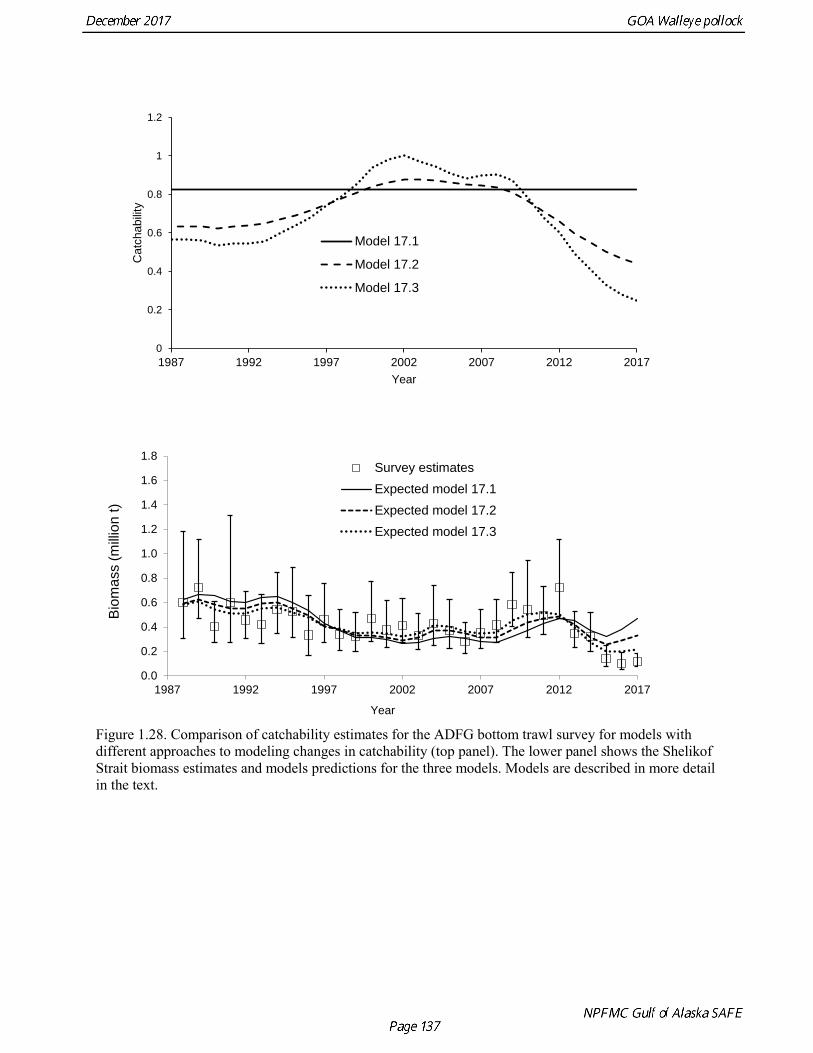
Figure 1.28. Comparison of catchability estimates for the ADFG bottom trawl survey for models with different approaches to modeling changes in catchability (top panel). The lower panel shows the Shelikof Strait biomass estimates and models predictions for the three models. Models are described in more detail in the text.

0.0

0.2

0.4

0.6

0.8

1.0

1.2

1.4

1.6

1.8

1987 1992 1997 2002 2007 2012 2017

Bio

mas

s (m

illion

t)

Year

Survey estimatesExpected model 17.1Expected model 17.2Expected model 17.3

0

0.2

0.4

0.6

0.8

1

1.2

1987 1992 1997 2002 2007 2012 2017

Cat

chab

ility

Year

Model 17.1

Model 17.2

Model 17.3

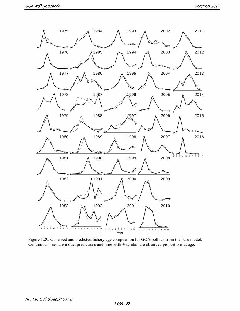
Figure 1.29. Observed and predicted fishery age composition for GOA pollock from the base model. Continuous lines are model predictions and lines with + symbol are observed proportions at age.

1975 1984 1993 2002 2011

1976 1985 1994 2003 2012

1977 1986 1995 2004 2013

1978 1987 1996 2005 2014

1979 1988 1997 2006 2015

1980 1989 1998 2007 2016

1981 1990 1999 2008

1982 1991 2000 2009

1983 1992 2001 2010

Age1 2 3 4 5 6 7 8 9 10 1 2 3 4 5 6 7 8 9 101 2 3 4 5 6 7 8 9 10 1 2 3 4 5 6 7 8 9 10

1 2 3 4 5 6 7 8 9 1 0

1 2 3 4 5 6 7 8 9 1 0

1 2 3 4 5 6 7 8 9 10

1 2 3 4 5 6 7 8 9 1 0

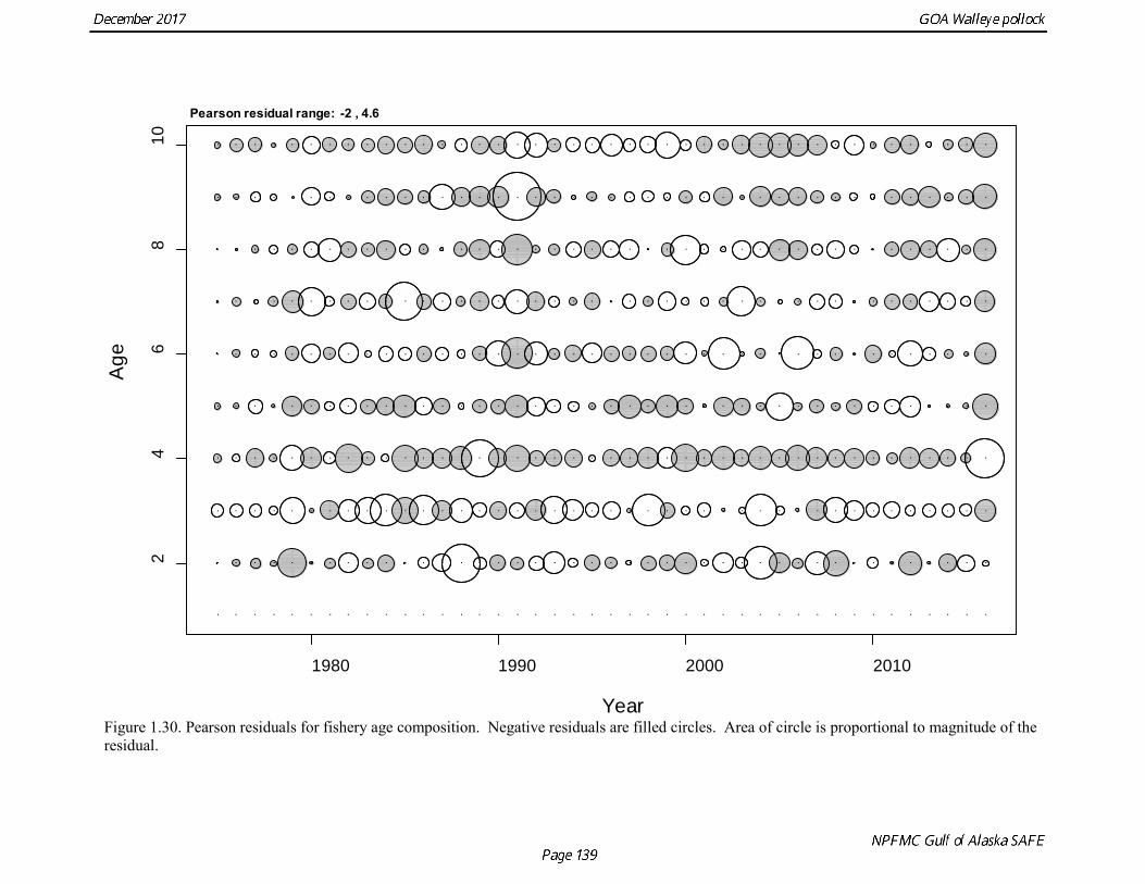
Figure 1.30. Pearson residuals for fishery age composition. Negative residuals are filled circles. Area of circle is proportional to magnitude of the residual.

1980 1990 2000 2010

24

68

10

Year

Age

Pearson residual range: -2 , 4.6

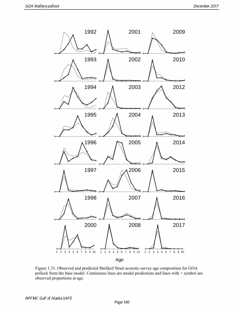
Figure 1.31. Observed and predicted Shelikof Strait acoustic survey age composition for GOA pollock from the base model. Continuous lines are model predictions and lines with + symbol are observed proportions at age.

1992 2001 2009

1993 2002 2010

1994 2003 2012

1995 2004 2013

1996 2005 2014

1997 2006 2015

1998 2007 2016

2000 2008 2017

Age

1 2 3 4 5 6 7 8 9 10 1 2 3 4 5 6 7 8 9 10 1 2 3 4 5 6 7 8 9 10

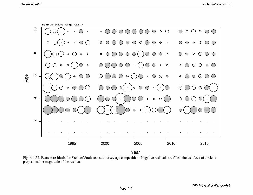
Figure 1.32. Pearson residuals for Shelikof Strait acoustic survey age composition. Negative residuals are filled circles. Area of circle is proportional to magnitude of the residual.

1995 2000 2005 2010 2015

24

68

10

Year

Age

Pearson residual range: -2.1 , 3

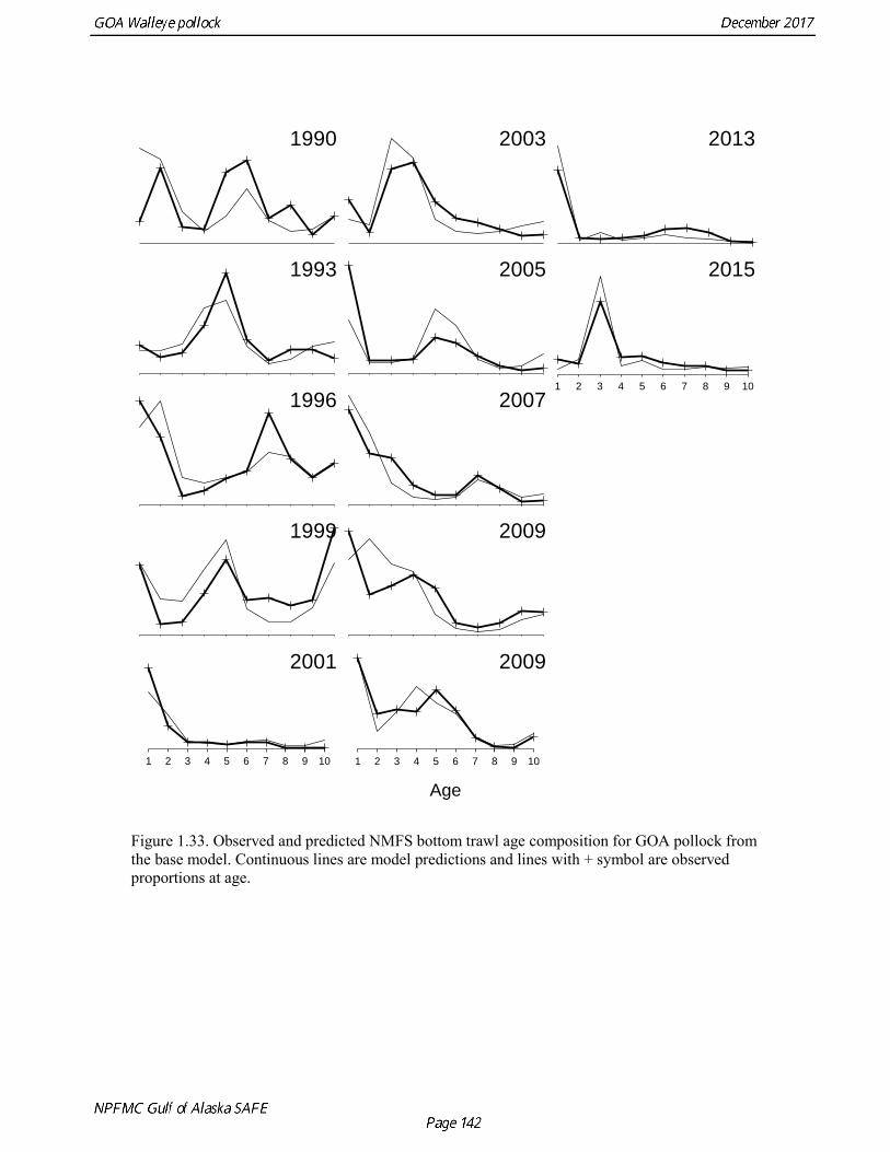
Figure 1.33. Observed and predicted NMFS bottom trawl age composition for GOA pollock from the base model. Continuous lines are model predictions and lines with + symbol are observed proportions at age.

1990 2003 2013

1993 2005 2015

1996 2007

1999 2009

2001 2009

Age

1 2 3 4 5 6 7 8 9 10 1 2 3 4 5 6 7 8 9 10

1 2 3 4 5 6 7 8 9 10

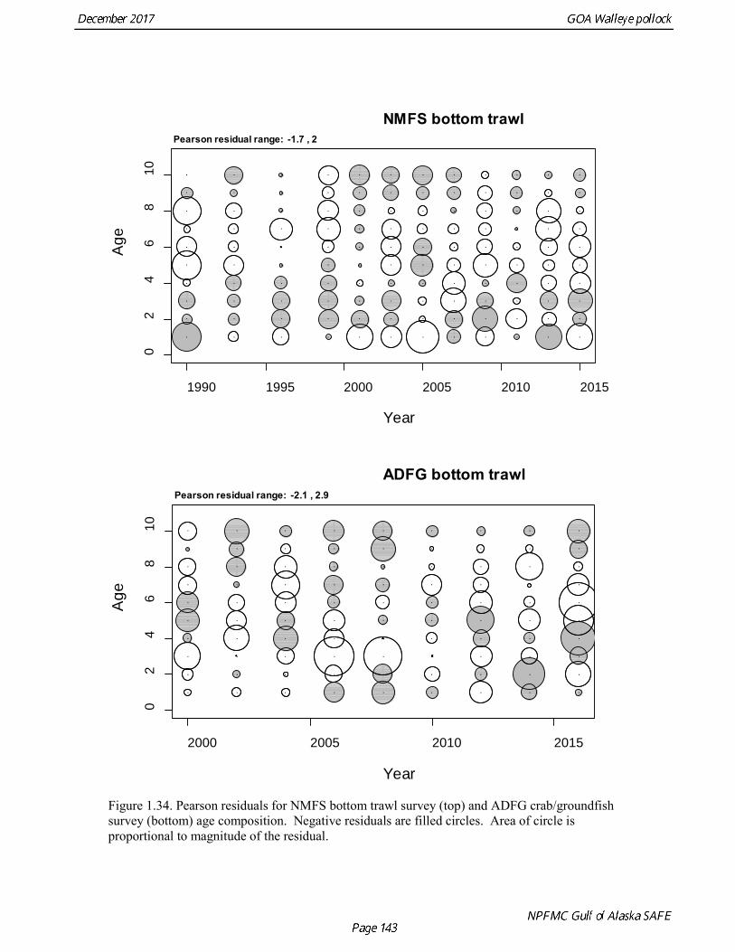
Figure 1.34. Pearson residuals for NMFS bottom trawl survey (top) and ADFG crab/groundfish survey (bottom) age composition. Negative residuals are filled circles. Area of circle is proportional to magnitude of the residual.

1990 1995 2000 2005 2010 2015

02

46

810

Year

Age

NMFS bottom trawl Pearson residual range: -1.7 , 2

2000 2005 2010 2015

02

46

810

Year

Age

ADFG bottom trawl Pearson residual range: -2.1 , 2.9

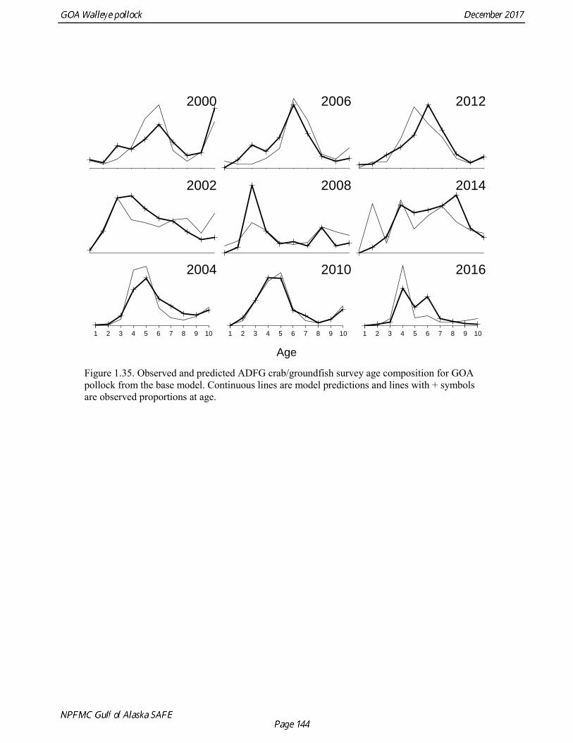
Figure 1.35. Observed and predicted ADFG crab/groundfish survey age composition for GOA pollock from the base model. Continuous lines are model predictions and lines with + symbols are observed proportions at age.

2000 2006 2012

2002 2008 2014

2004 2010 2016

Age

1 2 3 4 5 6 7 8 9 10 1 2 3 4 5 6 7 8 9 10 1 2 3 4 5 6 7 8 9 10

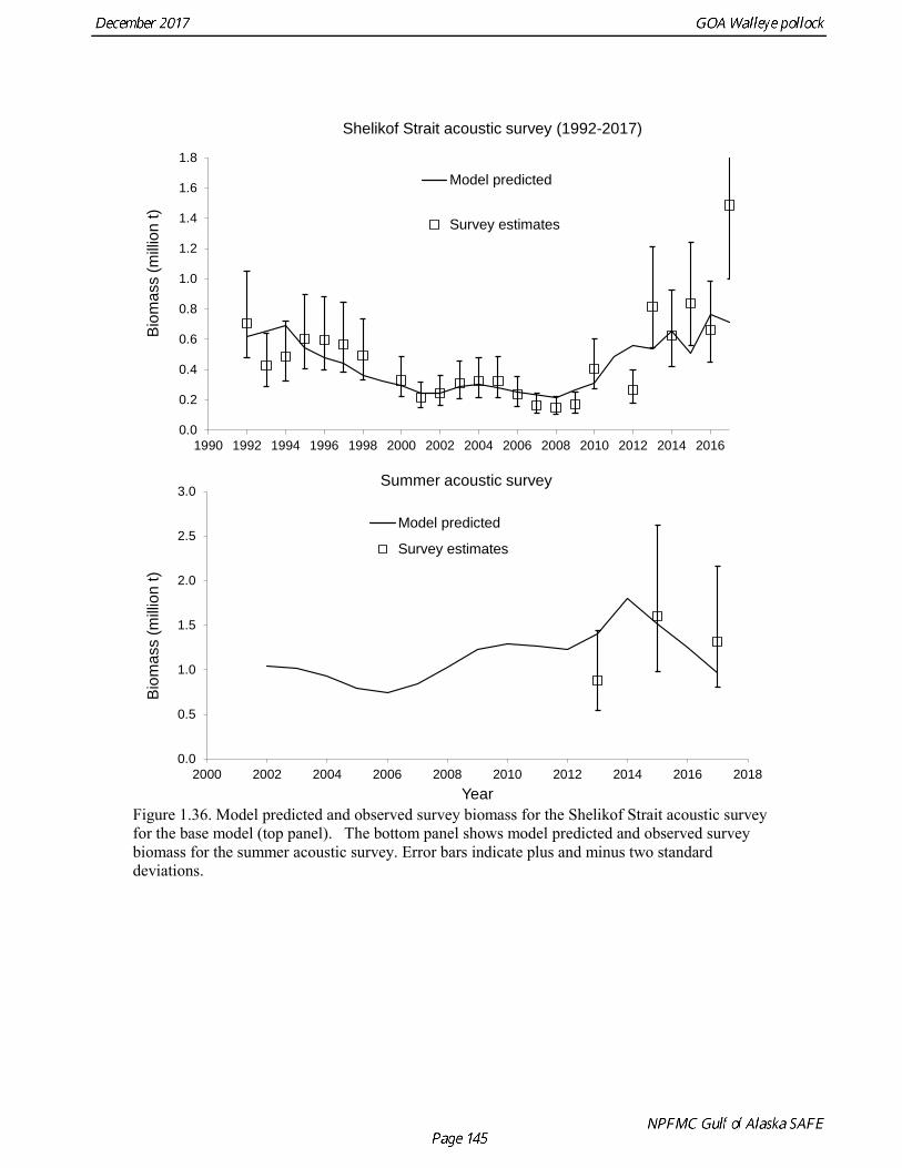
Figure 1.36. Model predicted and observed survey biomass for the Shelikof Strait acoustic survey for the base model (top panel). The bottom panel shows model predicted and observed survey biomass for the summer acoustic survey. Error bars indicate plus and minus two standard deviations.

0.0

0.2

0.4

0.6

0.8

1.0

1.2

1.4

1.6

1.8

1990 1992 1994 1996 1998 2000 2002 2004 2006 2008 2010 2012 2014 2016

Bio

mas

s (m

illion

t)Shelikof Strait acoustic survey (1992-2017)

Model predicted

Survey estimates

0.0

0.5

1.0

1.5

2.0

2.5

3.0

2000 2002 2004 2006 2008 2010 2012 2014 2016 2018

Bio

mas

s (m

illion

t)

Year

Summer acoustic survey

Model predicted

Survey estimates

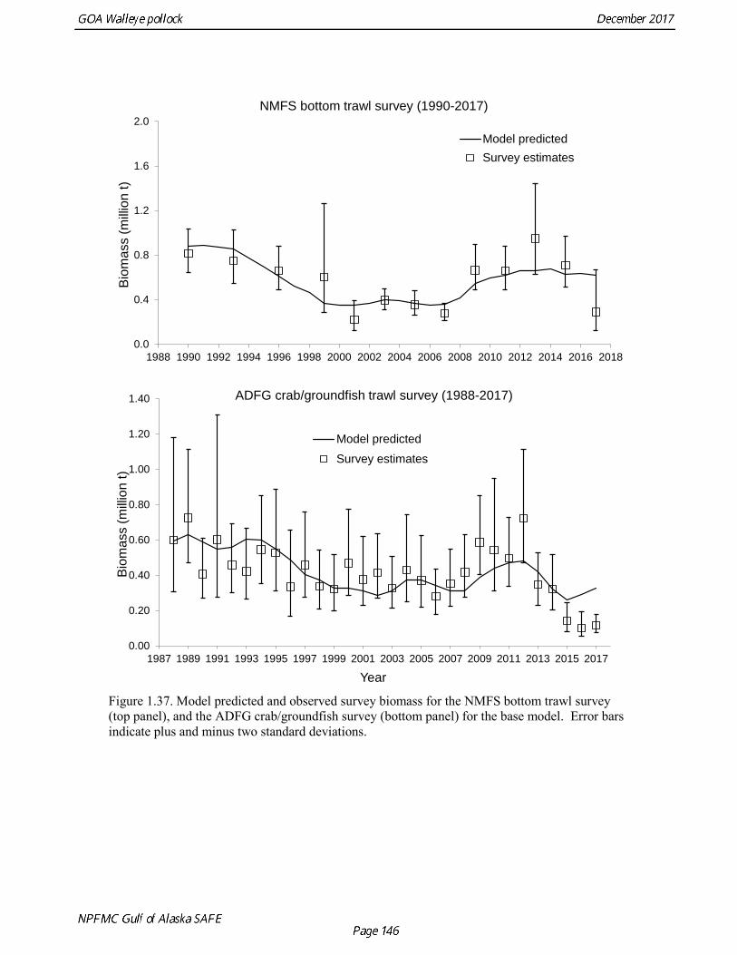
Figure 1.37. Model predicted and observed survey biomass for the NMFS bottom trawl survey (top panel), and the ADFG crab/groundfish survey (bottom panel) for the base model. Error bars indicate plus and minus two standard deviations.

0.0

0.4

0.8

1.2

1.6

2.0

1988 1990 1992 1994 1996 1998 2000 2002 2004 2006 2008 2010 2012 2014 2016 2018

Bio

mas

s (m

illion

t)NMFS bottom trawl survey (1990-2017)

Model predictedSurvey estimates

0.00

0.20

0.40

0.60

0.80

1.00

1.20

1.40

1987 1989 1991 1993 1995 1997 1999 2001 2003 2005 2007 2009 2011 2013 2015 2017

Bio

mas

s (m

illion

t)

Year

ADFG crab/groundfish trawl survey (1988-2017)

Model predicted

Survey estimates

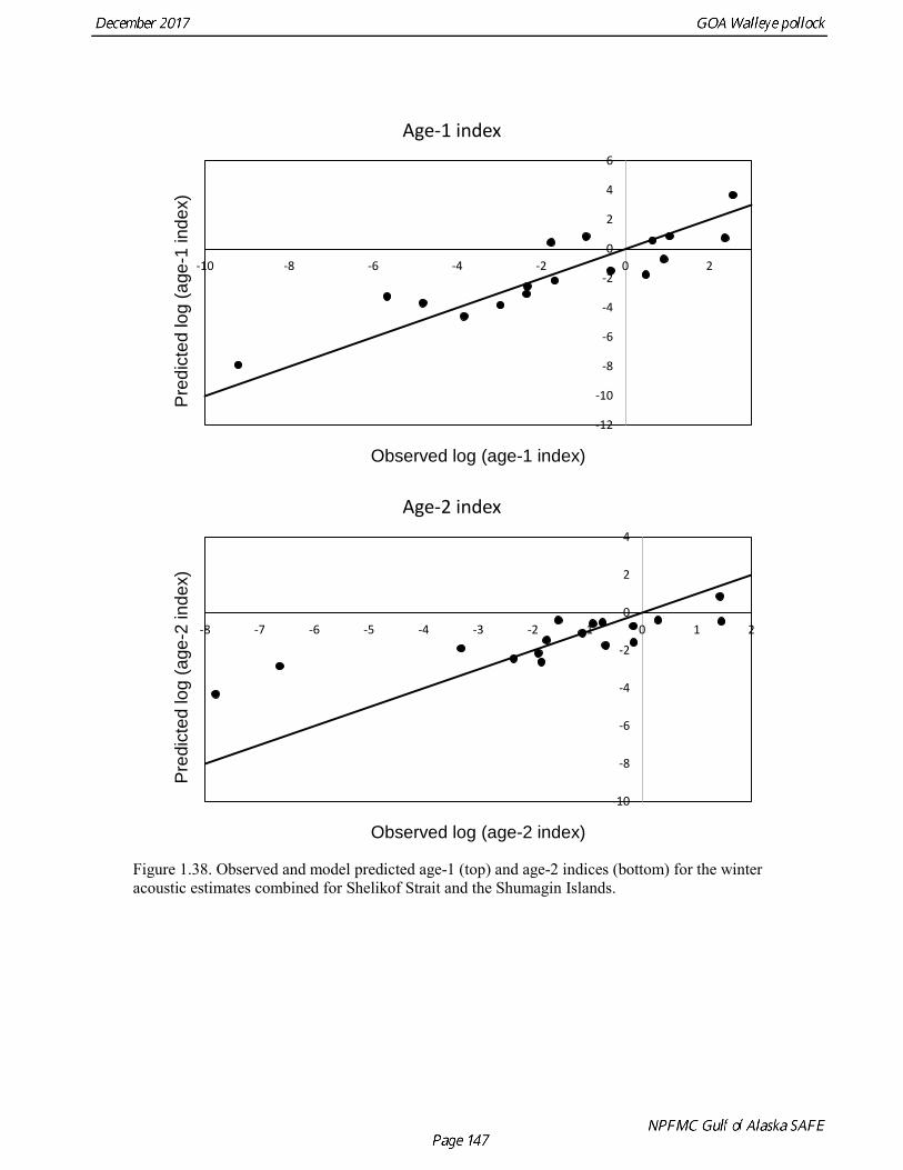
Figure 1.38. Observed and model predicted age-1 (top) and age-2 indices (bottom) for the winter acoustic estimates combined for Shelikof Strait and the Shumagin Islands.

-12

-10

-8

-6

-4

-2

0

2

4

6

-10 -8 -6 -4 -2 0 2

Pre

dict

ed lo

g (a

ge-1

inde

x)

Observed log (age-1 index)

Age-1 index

-10

-8

-6

-4

-2

0

2

4

-8 -7 -6 -5 -4 -3 -2 -1 0 1 2

Pre

dict

ed lo

g (a

ge-2

inde

x)

Observed log (age-2 index)

Age-2 index

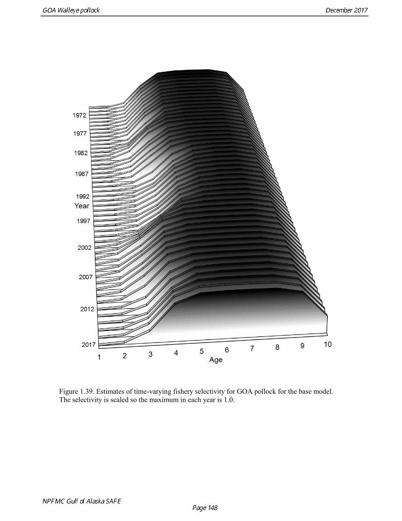
Figure 1.39. Estimates of time-varying fishery selectivity for GOA pollock for the base model. The selectivity is scaled so the maximum in each year is 1.0.

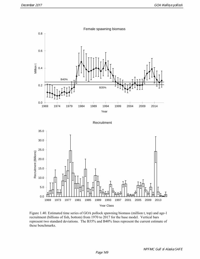
Figure 1.40. Estimated time series of GOA pollock spawning biomass (million t, top) and age-1 recruitment (billions of fish, bottom) from 1970 to 2017 for the base model. Vertical bars represent two standard deviations. The B35% and B40% lines represent the current estimate of these benchmarks.

0.0

0.2

0.4

0.6

0.8

1969 1974 1979 1984 1989 1994 1999 2004 2009 2014

Milli

on t

Year

Female spawning biomass

B40%

B35%

0.0

5.0

10.0

15.0

20.0

25.0

30.0

35.0

1969 1973 1977 1981 1985 1989 1993 1997 2001 2005 2009 2013

Rec

ruitm

ent (

Billio

ns)

Year Class

Recruitment

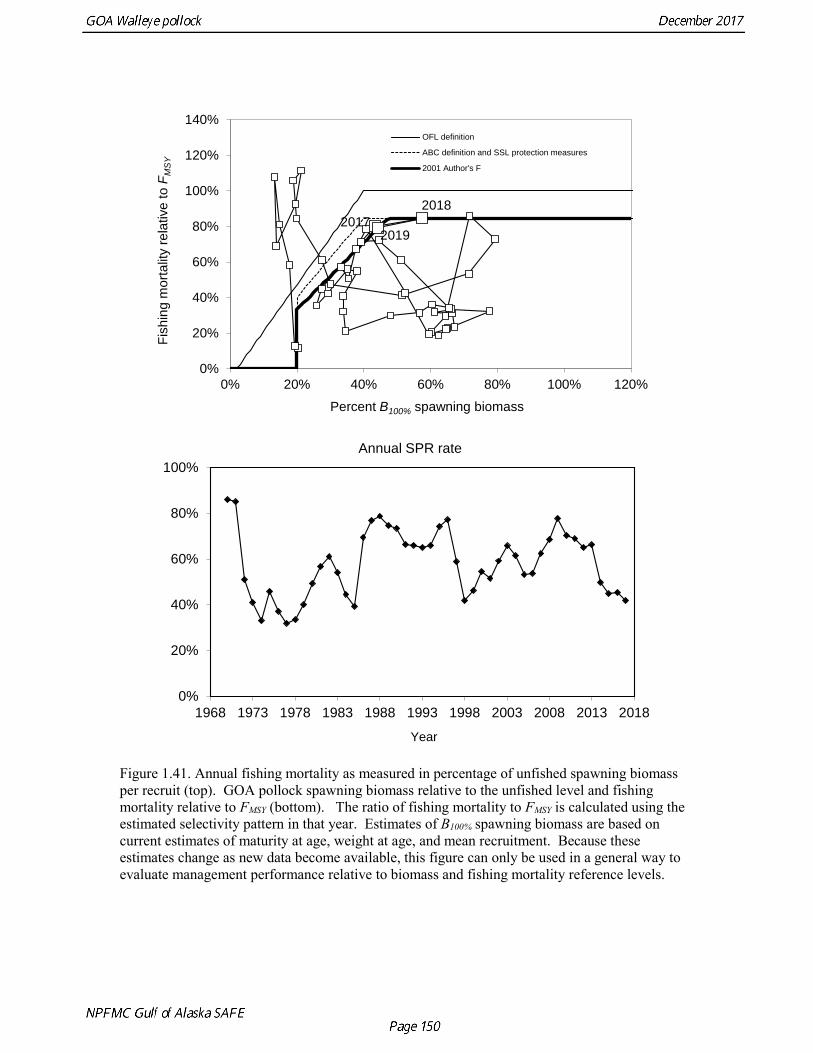
Figure 1.41. Annual fishing mortality as measured in percentage of unfished spawning biomass per recruit (top). GOA pollock spawning biomass relative to the unfished level and fishing mortality relative to FMSY (bottom). The ratio of fishing mortality to FMSY is calculated using the estimated selectivity pattern in that year. Estimates of B100% spawning biomass are based on current estimates of maturity at age, weight at age, and mean recruitment. Because these estimates change as new data become available, this figure can only be used in a general way to evaluate management performance relative to biomass and fishing mortality reference levels.

0%

20%

40%

60%

80%

100%

120%

140%

0% 20% 40% 60% 80% 100% 120%

Fish

ing

mor

talit

y re

lativ

e to

FM

SY

Percent B100% spawning biomass

OFL definition

ABC definition and SSL protection measures

2001 Author's F

20192017

2018

0%

20%

40%

60%

80%

100%

1968 1973 1978 1983 1988 1993 1998 2003 2008 2013 2018

Year

Annual SPR rate

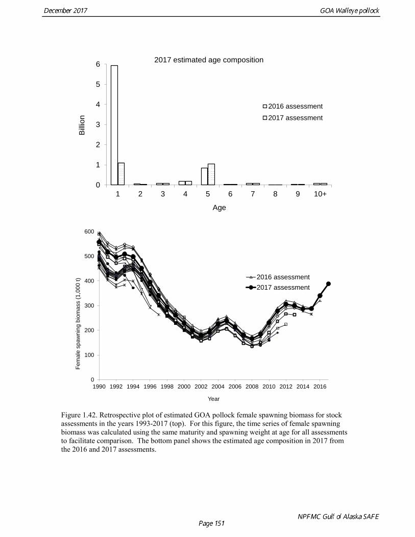
Figure 1.42. Retrospective plot of estimated GOA pollock female spawning biomass for stock assessments in the years 1993-2017 (top). For this figure, the time series of female spawning biomass was calculated using the same maturity and spawning weight at age for all assessments to facilitate comparison. The bottom panel shows the estimated age composition in 2017 from the 2016 and 2017 assessments.

0

1

2

3

4

5

6

1 2 3 4 5 6 7 8 9 10+

Billi

on

Age

2017 estimated age composition

2016 assessment

2017 assessment

0

100

200

300

400

500

600

1990 1992 1994 1996 1998 2000 2002 2004 2006 2008 2010 2012 2014 2016

Fem

ale

spaw

ning

bio

mas

s (1

,000

t)

Year

2016 assessment2017 assessment

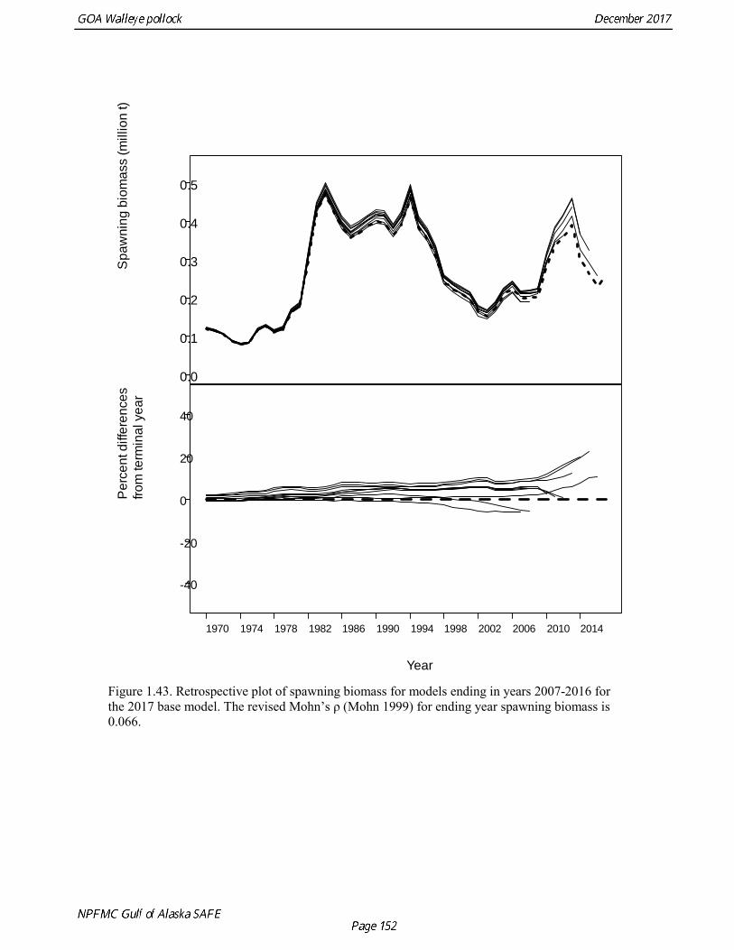
Figure 1.43. Retrospective plot of spawning biomass for models ending in years 2007-2016 for the 2017 base model. The revised Mohn’s ρ (Mohn 1999) for ending year spawning biomass is 0.066.

0.0

0.1

0.2

0.3

0.4

0.5

Spa

wni

ng b

iom

ass

(mill

ion

t)

-40

-20

0

20

40

Per

cent

diff

eren

ces

from

term

inal

yea

r

1970 1974 1978 1982 1986 1990 1994 1998 2002 2006 2010 2014

Year

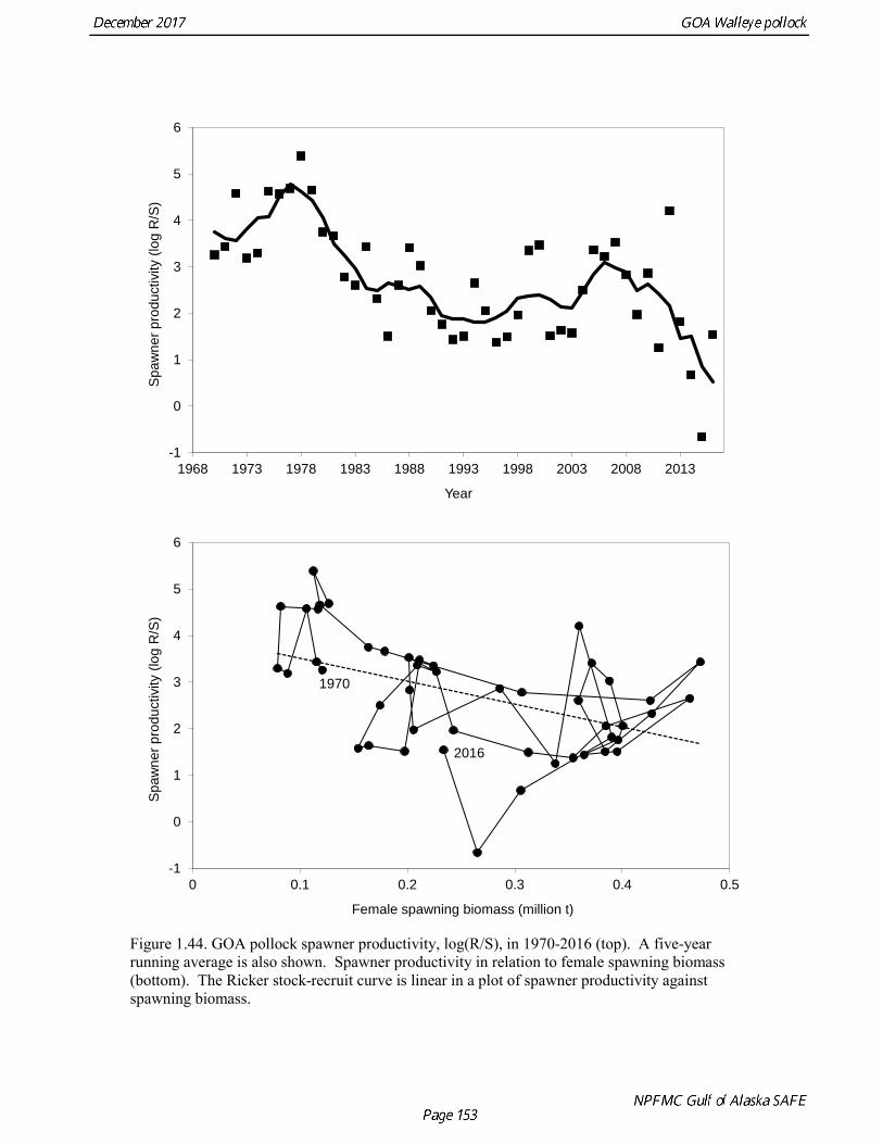
Figure 1.44. GOA pollock spawner productivity, log(R/S), in 1970-2016 (top). A five-year running average is also shown. Spawner productivity in relation to female spawning biomass (bottom). The Ricker stock-recruit curve is linear in a plot of spawner productivity against spawning biomass.

-1

0

1

2

3

4

5

6

1968 1973 1978 1983 1988 1993 1998 2003 2008 2013

Spa

wne

r pro

duct

ivity

(log

R/S

)

Year

-1

0

1

2

3

4

5

6

0 0.1 0.2 0.3 0.4 0.5

Spa

wne

r pro

duct

ivity

(log

R/S

)

Female spawning biomass (million t)

1970

2016

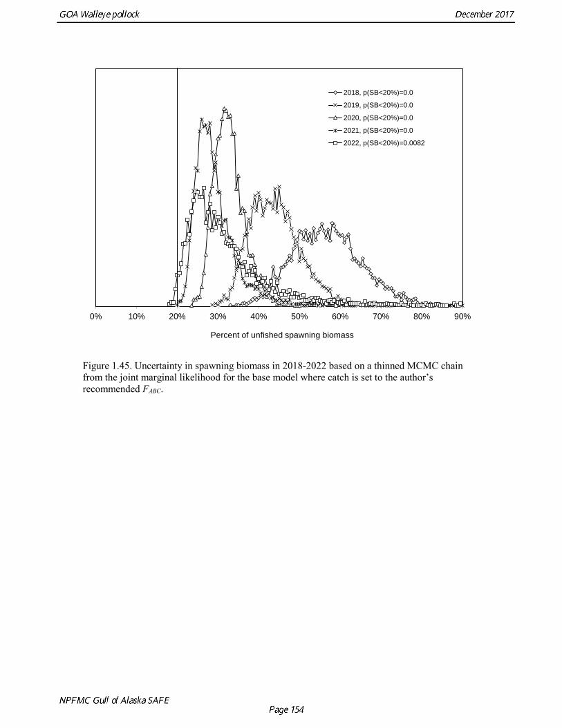
Figure 1.45. Uncertainty in spawning biomass in 2018-2022 based on a thinned MCMC chain from the joint marginal likelihood for the base model where catch is set to the author’s recommended FABC.

0% 10% 20% 30% 40% 50% 60% 70% 80% 90%

Percent of unfished spawning biomass

2018, p(SB<20%)=0.0

2019, p(SB<20%)=0.0

2020, p(SB<20%)=0.0

2021, p(SB<20%)=0.0

2022, p(SB<20%)=0.0082

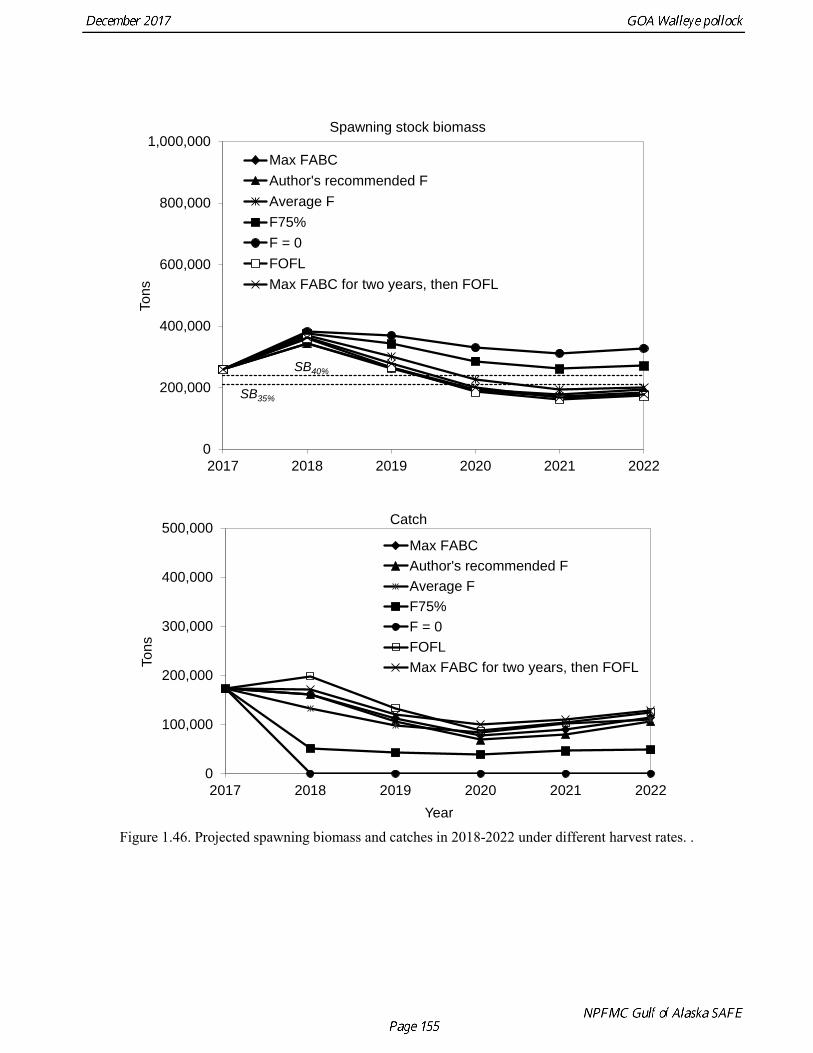
Figure 1.46. Projected spawning biomass and catches in 2018-2022 under different harvest rates. .

0

200,000

400,000

600,000

800,000

1,000,000

2017 2018 2019 2020 2021 2022

Tons

Spawning stock biomass

Max FABCAuthor's recommended FAverage FF75%F = 0FOFLMax FABC for two years, then FOFL

SB40%

SB35%

0

100,000

200,000

300,000

400,000

500,000

2017 2018 2019 2020 2021 2022

Tons

Year

Catch

Max FABCAuthor's recommended FAverage FF75%F = 0FOFLMax FABC for two years, then FOFL

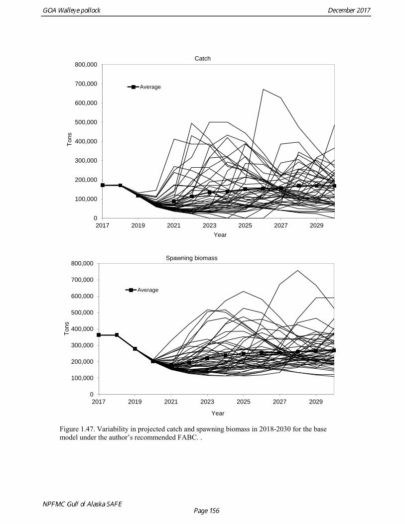
Figure 1.47. Variability in projected catch and spawning biomass in 2018-2030 for the base model under the author’s recommended FABC. .

0

100,000

200,000

300,000

400,000

500,000

600,000

700,000

800,000

2017 2019 2021 2023 2025 2027 2029

Tons

Year

Catch

Average

0

100,000

200,000

300,000

400,000

500,000

600,000

700,000

800,000

2017 2019 2021 2023 2025 2027 2029

Tons

Year

Spawning biomass

Average

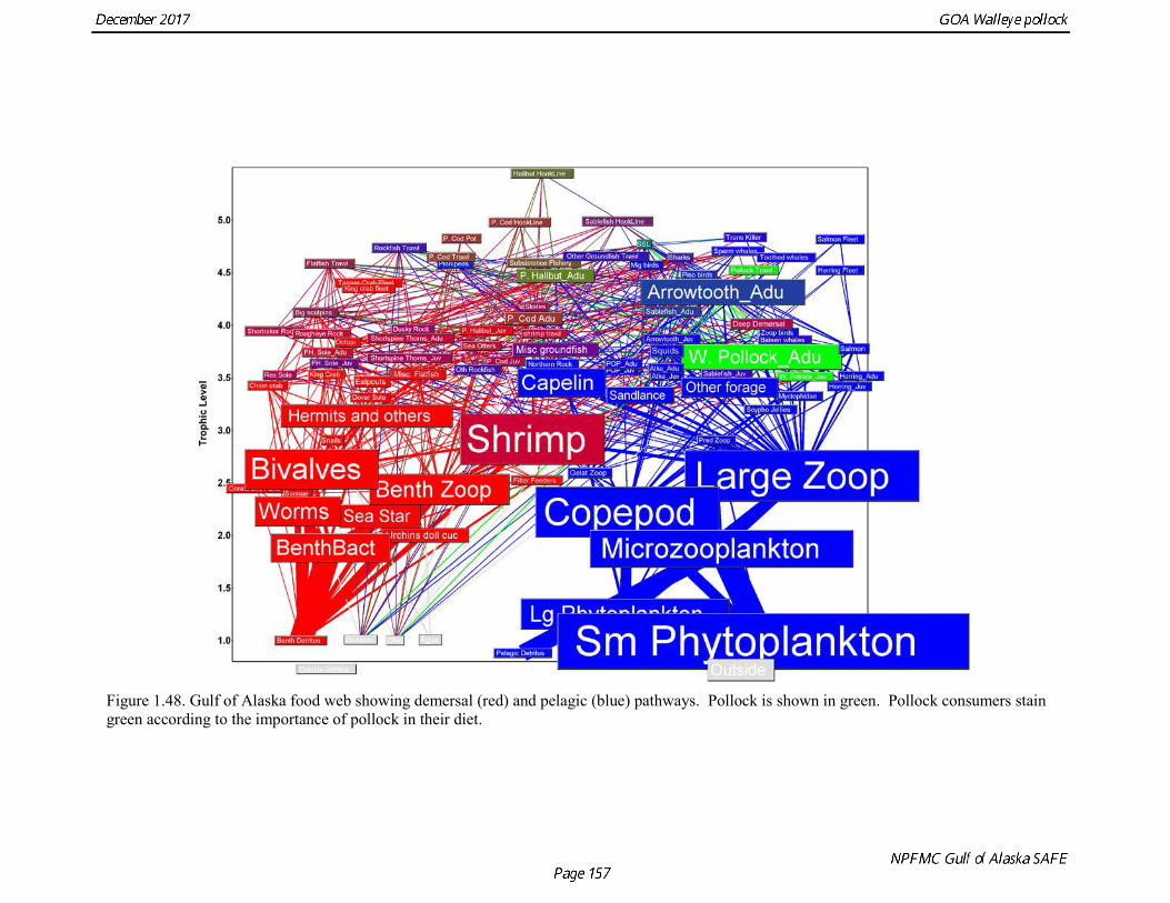
Figure 1.48. Gulf of Alaska food web showing demersal (red) and pelagic (blue) pathways. Pollock is shown in green. Pollock consumers stain green according to the importance of pollock in their diet.

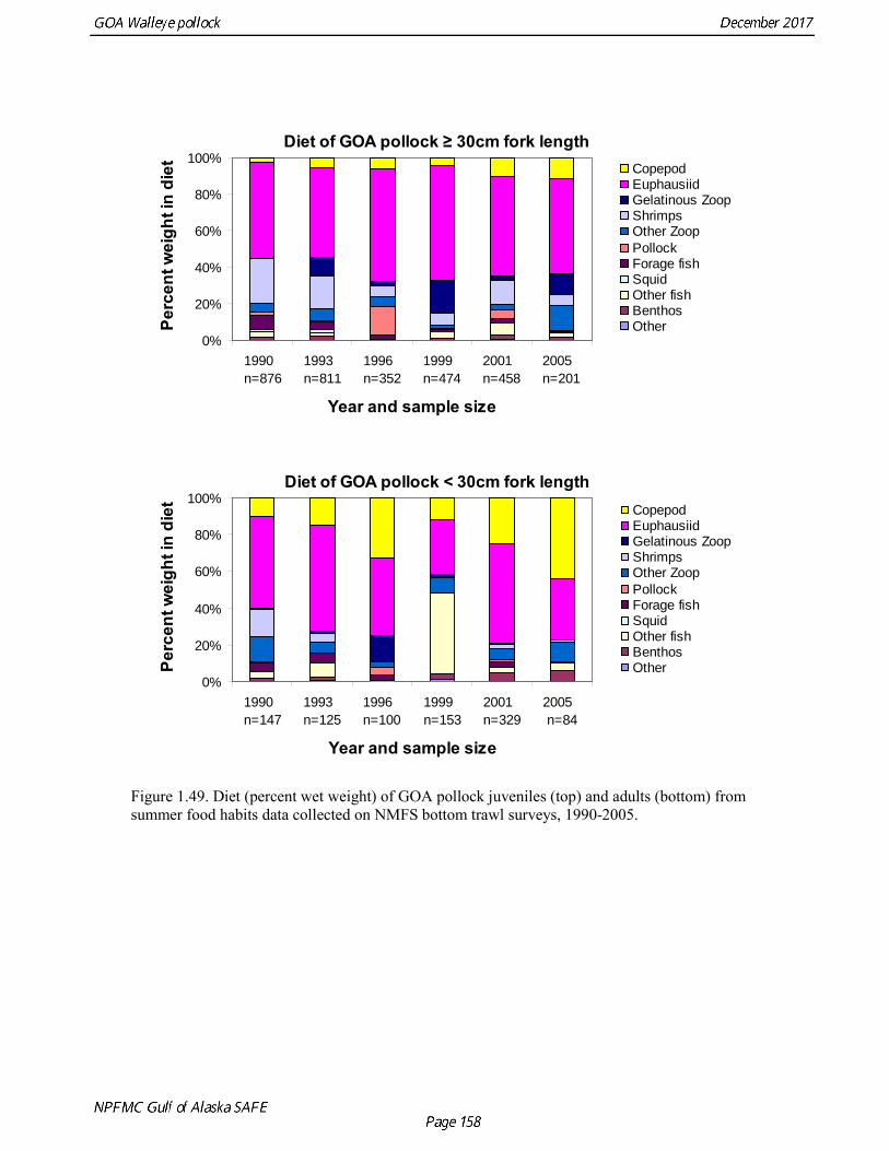
Figure 1.49. Diet (percent wet weight) of GOA pollock juveniles (top) and adults (bottom) from summer food habits data collected on NMFS bottom trawl surveys, 1990-2005.

Diet of GOA pollock ≥ 30cm fork length

0%

20%

40%

60%

80%

100%

1990 n=876

1993 n=811

1996 n=352

1999 n=474

2001 n=458

2005 n=201

Year and sample size

Perc

ent w

eigh

t in

diet Copepod

EuphausiidGelatinous ZoopShrimpsOther ZoopPollockForage fishSquidOther fishBenthosOther

Diet of GOA pollock < 30cm fork length

0%

20%

40%

60%

80%

100%

1990 n=147

1993 n=125

1996 n=100

1999 n=153

2001 n=329

2005 n=84

Year and sample size

Perc

ent w

eigh

t in

diet CopepodEuphausiidGelatinous ZoopShrimpsOther ZoopPollockForage fishSquidOther fishBenthosOther

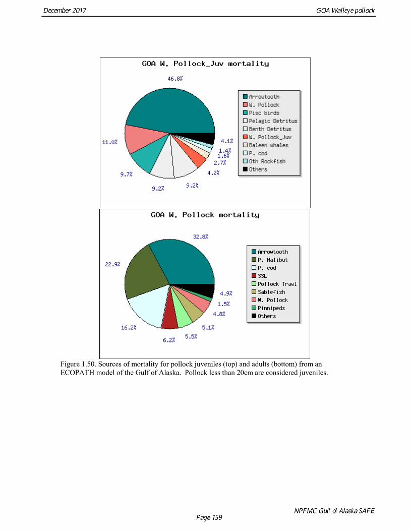
Figure 1.50. Sources of mortality for pollock juveniles (top) and adults (bottom) from an ECOPATH model of the Gulf of Alaska. Pollock less than 20cm are considered juveniles.

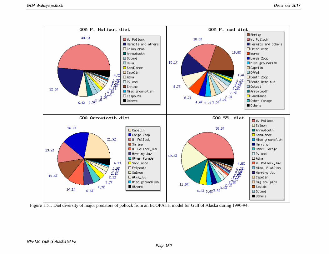
Figure 1.51. Diet diversity of major predators of pollock from an ECOPATH model for Gulf of Alaska during 1990-94.

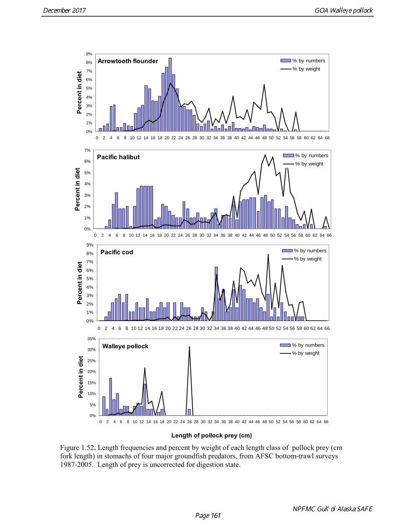
Figure 1.52. Length frequencies and percent by weight of each length class of pollock prey (cm fork length) in stomachs of four major groundfish predators, from AFSC bottom-trawl surveys 1987-2005. Length of prey is uncorrected for digestion state.

Arrowtooth flounder

0%

1%

2%

3%

4%

5%

6%

7%

8%

9%

0 2 4 6 8 10 12 14 16 18 20 22 24 26 28 30 32 34 36 38 40 42 44 46 48 50 52 54 56 58 60 62 64 66

Perc

ent i

n di

et

% by numbers% by weight

Pacific halibut

0%

1%

2%

3%

4%

5%

6%

7%

0 2 4 6 8 10 12 14 16 18 20 22 24 26 28 30 32 34 36 38 40 42 44 46 48 50 52 54 56 58 60 62 64 66

Perc

ent i

n di

et

% by numbers% by weight

Pacific cod

0%

1%

2%

3%

4%

5%

6%

7%

8%

9%

0 2 4 6 8 10 12 14 16 18 20 22 24 26 28 30 32 34 36 38 40 42 44 46 48 50 52 54 56 58 60 62 64 66

Perc

ent i

n di

et

% by numbers% by weight

Walleye pollock

0%

5%

10%

15%

20%

25%

30%

35%

0 2 4 6 8 10 12 14 16 18 20 22 24 26 28 30 32 34 36 38 40 42 44 46 48 50 52 54 56 58 60 62 64 66

Length of pollock prey (cm)

Perc

ent i

n di

et

% by numbers% by weight

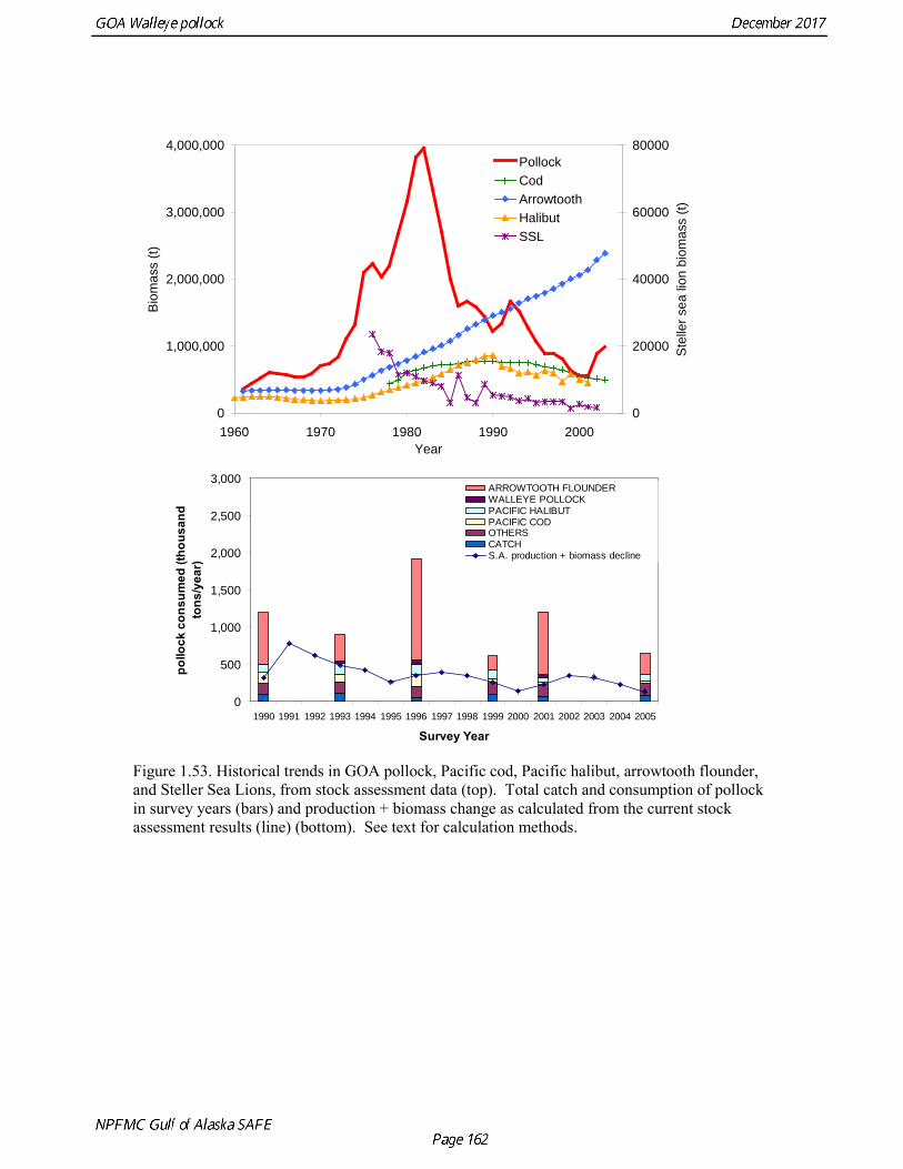
Figure 1.53. Historical trends in GOA pollock, Pacific cod, Pacific halibut, arrowtooth flounder, and Steller Sea Lions, from stock assessment data (top). Total catch and consumption of pollock in survey years (bars) and production + biomass change as calculated from the current stock assessment results (line) (bottom). See text for calculation methods.

0

1,000,000

2,000,000

3,000,000

4,000,000

1960 1970 1980 1990 2000Year

Bio

mas

s (t)

0

20000

40000

60000

80000

Ste

ller s

ea li

on b

iom

ass

(t)

PollockCodArrowtoothHalibutSSL

0

500

1,000

1,500

2,000

2,500

3,000

1990 1991 1992 1993 1994 1995 1996 1997 1998 1999 2000 2001 2002 2003 2004 2005

Survey Year

pollo

ck c

onsu

med

(tho

usan

d to

ns/y

ear)

ARROWTOOTH FLOUNDERWALLEYE POLLOCKPACIFIC HALIBUTPACIFIC CODOTHERSCATCHS.A. production + biomass decline

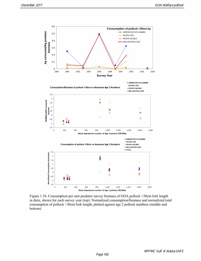
Figure 1.54. Consumption per unit predator survey biomass of GOA pollock <30cm fork length in diets, shown for each survey year (top). Normalized consumption/biomass and normalized total consumption of pollock <30cm fork length, plotted against age 2 pollock numbers (middle and bottom).

Consumption of pollock <30cm by

0

0.1

0.2

0.3

0.4

0.5

0.6

1988 1990 1992 1994 1996 1998 2000 2002 2004 2006

Survey Year

kg c

onsu

med

/kg

pred

ator

bi

omas

s

ARROWTOOTH FLOUNDER

PACIFIC COD

PACIFIC HALIBUT

WALLEYE POLLOCK

Consumption/Biomass of pollock <30cm vs Assessed Age 2 Numbers

-1.5

-1

-0.5

0

0.5

1

1.5

2

2.5

0 200 400 600 800 1,000 1,200 1,400 1,600 1,800

Stock Assessment number of Age 2 pollock (100,000s)

NORM

ALIZ

ED c

ons/

pred

bi

omas

s

ARROWTOOTH FLOUNDERPACIFIC CODPACIFIC HALIBUTWALLEYE POLLOCK

Consumption of pollock <30cm vs Assessed Age 2 Numbers

-1.5

-1

-0.5

0

0.5

1

1.5

2

2.5

0 200 400 600 800 1,000 1,200 1,400 1,600 1,800

Stock Assessment number of Age 2 pollock (100,000s)

Norm

aliz

ed C

onsu

mpt

ion

(tons

/yea

r)

ARROWTOOTH FLOUNDERPACIFIC CODPACIFIC HALIBUTWALLEYE POLLOCKTOTAL

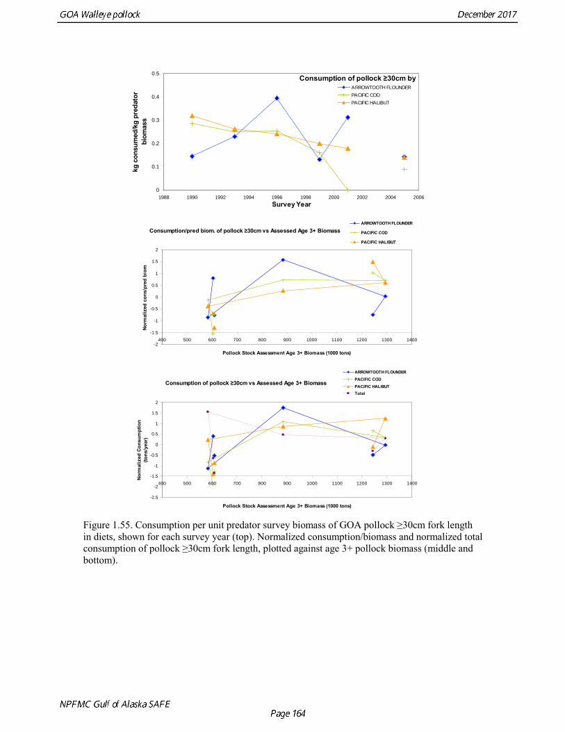
Figure 1.55. Consumption per unit predator survey biomass of GOA pollock ≥30cm fork length in diets, shown for each survey year (top). Normalized consumption/biomass and normalized total consumption of pollock ≥30cm fork length, plotted against age 3+ pollock biomass (middle and bottom).

Consumption of pollock ≥30cm by

0

0.1

0.2

0.3

0.4

0.5

1988 1990 1992 1994 1996 1998 2000 2002 2004 2006Survey Year

kg c

onsu

med

/kg

pred

ator

bi

omas

s

ARROWTOOTH FLOUNDERPACIFIC CODPACIFIC HALIBUT

Consumption/pred biom. of pollock ≥30cm vs Assessed Age 3+ Biomass

-2

-1.5

-1

-0.5

0

0.5

1

1.5

2

400 500 600 700 800 900 1000 1100 1200 1300 1400

Pollock Stock Assessment Age 3+ Biomass (1000 tons)

Norm

aliz

ed c

ons/

pred

bio

m

ARROWTOOTH FLOUNDER

PACIFIC COD

PACIFIC HALIBUT

Consumption of pollock ≥30cm vs Assessed Age 3+ Biomass

-2.5

-2

-1.5

-1

-0.5

0

0.5

1

1.5

2

400 500 600 700 800 900 1000 1100 1200 1300 1400

Pollock Stock Assessment Age 3+ Biomass (1000 tons)

Norm

aliz

ed C

onsu

mpt

ion

(tons

/yea

r)

ARROWTOOTH FLOUNDERPACIFIC CODPACIFIC HALIBUTTotal

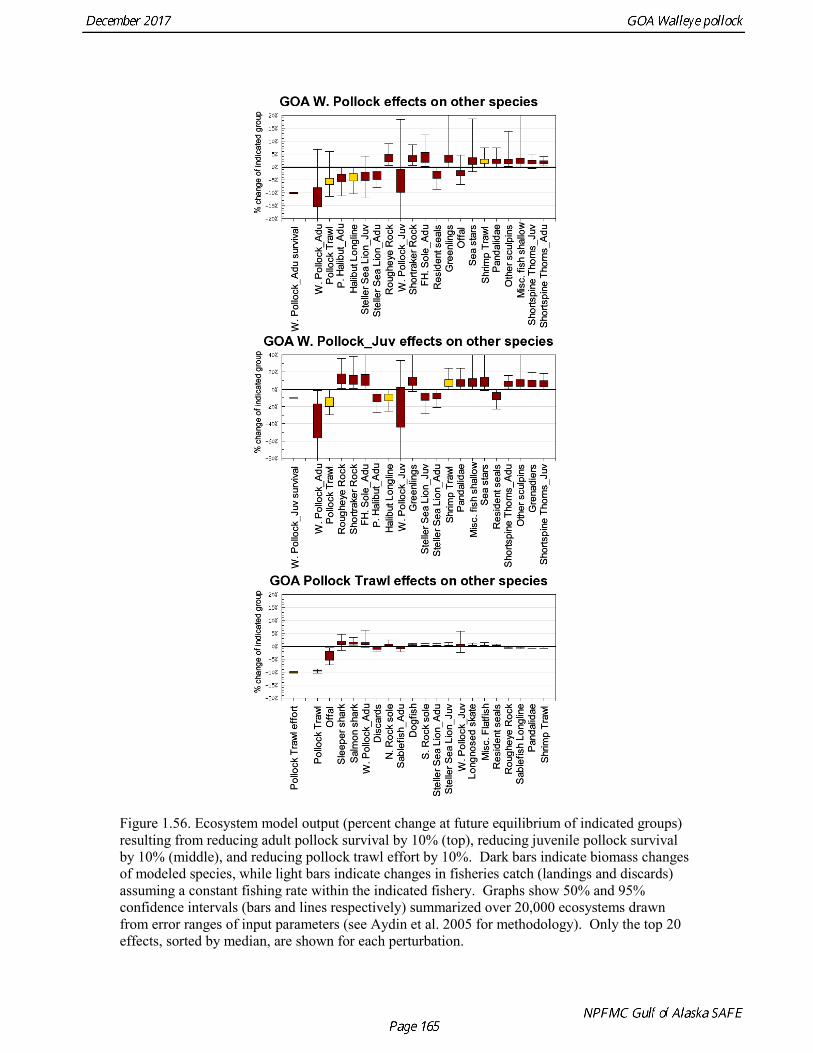
Figure 1.56. Ecosystem model output (percent change at future equilibrium of indicated groups) resulting from reducing adult pollock survival by 10% (top), reducing juvenile pollock survival by 10% (middle), and reducing pollock trawl effort by 10%. Dark bars indicate biomass changes of modeled species, while light bars indicate changes in fisheries catch (landings and discards) assuming a constant fishing rate within the indicated fishery. Graphs show 50% and 95% confidence intervals (bars and lines respectively) summarized over 20,000 ecosystems drawn from error ranges of input parameters (see Aydin et al. 2005 for methodology). Only the top 20 effects, sorted by median, are shown for each perturbation.

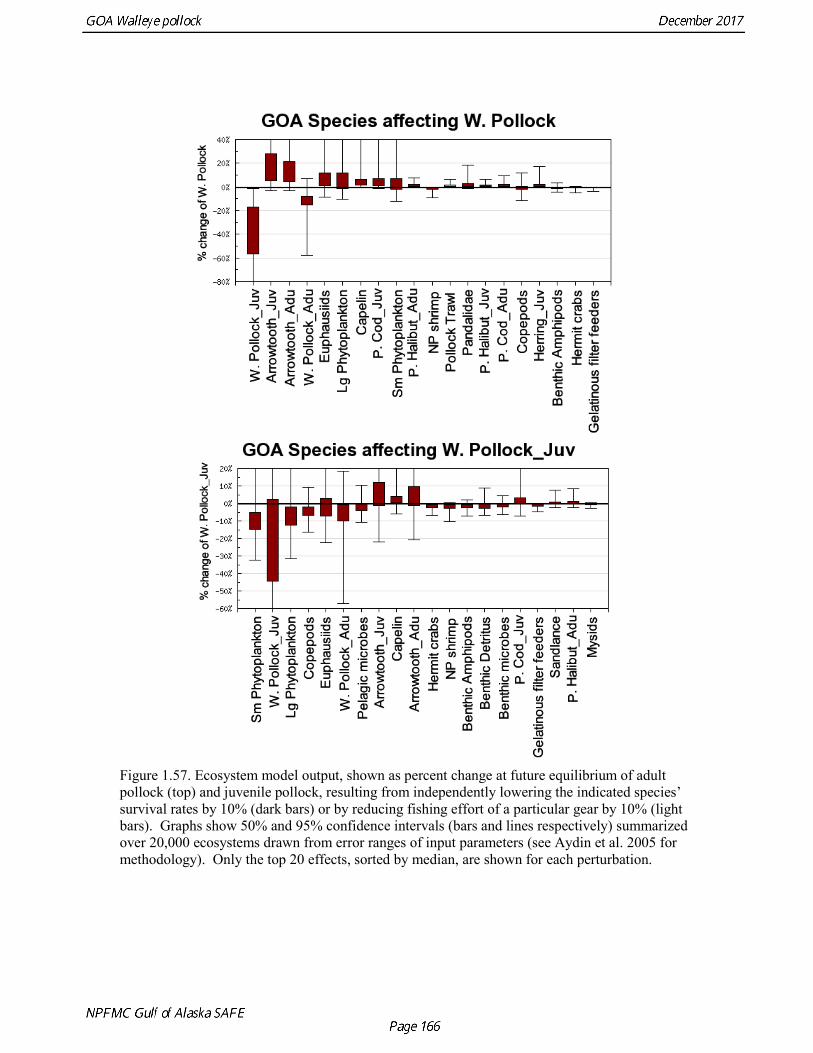
Figure 1.57. Ecosystem model output, shown as percent change at future equilibrium of adult pollock (top) and juvenile pollock, resulting from independently lowering the indicated species’ survival rates by 10% (dark bars) or by reducing fishing effort of a particular gear by 10% (light bars). Graphs show 50% and 95% confidence intervals (bars and lines respectively) summarized over 20,000 ecosystems drawn from error ranges of input parameters (see Aydin et al. 2005 for methodology). Only the top 20 effects, sorted by median, are shown for each perturbation.

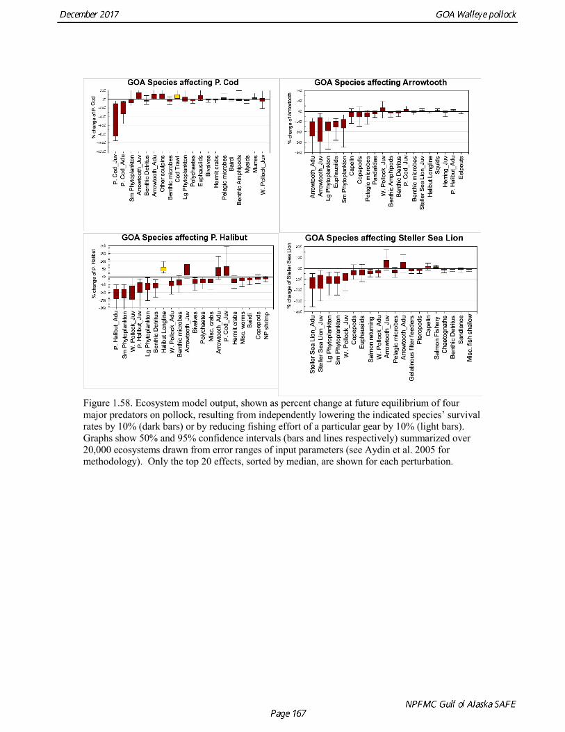
Figure 1.58. Ecosystem model output, shown as percent change at future equilibrium of four major predators on pollock, resulting from independently lowering the indicated species’ survival rates by 10% (dark bars) or by reducing fishing effort of a particular gear by 10% (light bars). Graphs show 50% and 95% confidence intervals (bars and lines respectively) summarized over 20,000 ecosystems drawn from error ranges of input parameters (see Aydin et al. 2005 for methodology). Only the top 20 effects, sorted by median, are shown for each perturbation.

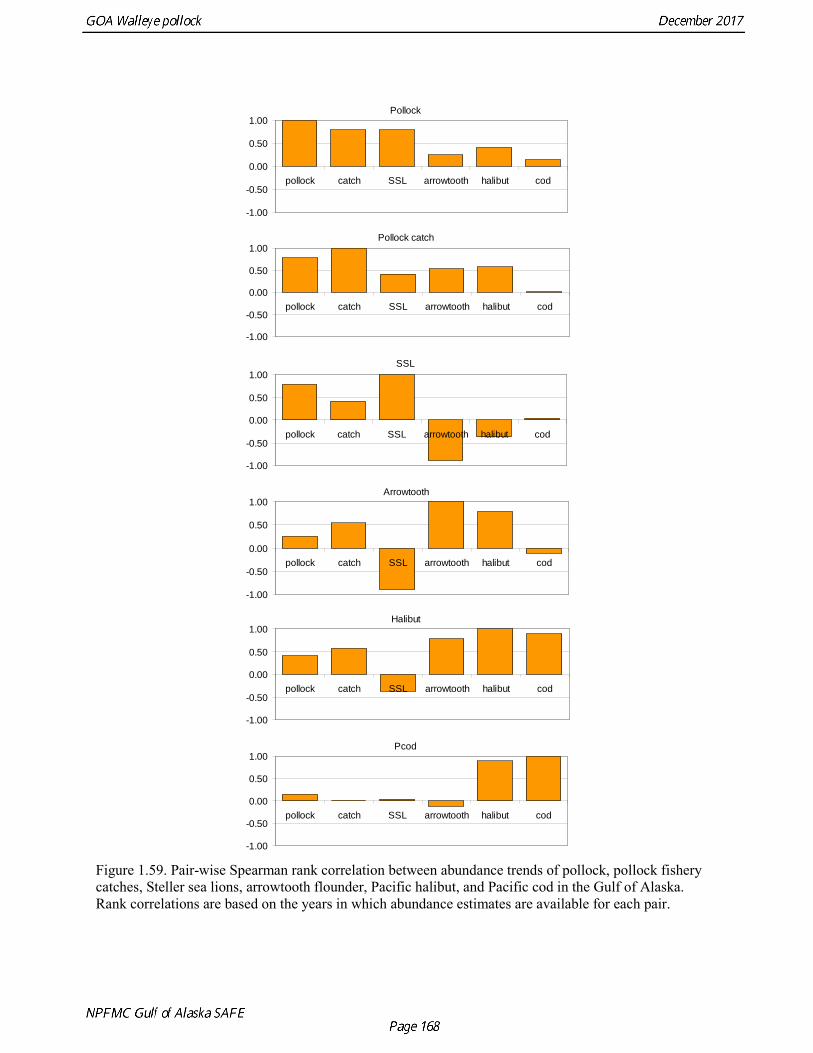
Figure 1.59. Pair-wise Spearman rank correlation between abundance trends of pollock, pollock fishery catches, Steller sea lions, arrowtooth flounder, Pacific halibut, and Pacific cod in the Gulf of Alaska. Rank correlations are based on the years in which abundance estimates are available for each pair.

Arrowtooth

-1.00

-0.50

0.00

0.50

1.00

pollock catch SSL arrowtooth halibut cod

Halibut

-1.00

-0.50

0.00

0.50

1.00

pollock catch SSL arrowtooth halibut cod

Pollock

-1.00

-0.50

0.00

0.50

1.00

pollock catch SSL arrowtooth halibut cod

Pollock catch

-1.00

-0.50

0.00

0.50

1.00

pollock catch SSL arrowtooth halibut cod

SSL

-1.00

-0.50

0.00

0.50

1.00

pollock catch SSL arrowtooth halibut cod

Pcod

-1.00

-0.50

0.00

0.50

1.00

pollock catch SSL arrowtooth halibut cod

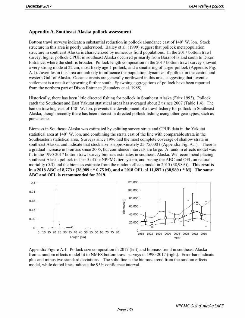
Appendix A. Southeast Alaska pollock assessment

Bottom trawl surveys indicate a substantial reduction in pollock abundance east of 140° W. lon. Stock structure in this area is poorly understood. Bailey et al. (1999) suggest that pollock metapopulation structure in southeast Alaska is characterized by numerous fiord populations. In the 2017 bottom trawl survey, higher pollock CPUE in southeast Alaska occurred primarily from Baranof Island south to Dixon Entrance, where the shelf is broader. Pollock length composition in the 2017 bottom trawl survey showed a very strong mode at 22 cm, most likely age-1 pollock, and a smattering of larger pollock (Appendix Fig. A.1). Juveniles in this area are unlikely to influence the population dynamics of pollock in the central and western Gulf of Alaska. Ocean currents are generally northward in this area, suggesting that juvenile settlement is a result of spawning further south. Spawning aggregations of pollock have been reported from the northern part of Dixon Entrance (Saunders et al. 1988). Historically, there has been little directed fishing for pollock in Southeast Alaska (Fritz 1993). Pollock catch the Southeast and East Yakutat statistical areas has averaged about 2 t since 2007 (Table 1.4). The ban on trawling east of 140° W. lon. prevents the development of a trawl fishery for pollock in Southeast Alaska, though recently there has been interest in directed pollock fishing using other gear types, such as purse seine. Biomass in Southeast Alaska was estimated by splitting survey strata and CPUE data in the Yakutat statistical area at 140° W. lon. and combining the strata east of the line with comparable strata in the Southeastern statistical area. Surveys since 1996 had the most complete coverage of shallow strata in southeast Alaska, and indicate that stock size is approximately 25-75,000 t (Appendix Fig. A.1). There is a gradual increase in biomass since 2005, but confidence intervals are large. A random effects model was fit to the 1990-2017 bottom trawl survey biomass estimates in southeast Alaska. We recommend placing southeast Alaska pollock in Tier 5 of the NPFMC tier system, and basing the ABC and OFL on natural mortality (0.3) and the biomass estimate from the random effects model in 2015 (38,989 t). This results in a 2018 ABC of 8,773 t (38,989 t * 0.75 M), and a 2018 OFL of 11,697 t (38,989 t * M). The same ABC and OFL is recommended for 2019.

Appendix Figure A.1. Pollock size composition in 2017 (left) and biomass trend in southeast Alaska from a random effects model fit to NMFS bottom trawl surveys in 1990-2017 (right). Error bars indicate plus and minus two standard deviations. The solid line is the biomass trend from the random effects model, while dotted lines indicate the 95% confidence interval.

0

20,000

40,000

60,000

80,000

100,000

120,000

1988 1992 1996 2000 2004 2008 2012 2016

Biom

ass

(t)

Year

0

0.06

0.12

0.18

0.24

0.3

5 10 15 20 25 30 35 40 45 50 55 60 65 70 75 80Length (cm)

Appendix B. GOA pollock stock assessment model

Population dynamics The age-structured model for pollock describes the relationships between population numbers by age and year. The modeled population includes individuals from age 1 to age 10, with age 10 defined as a “plus” group, i.e., all individuals age 10 and older. The model extends from 1970 to 2017 (48 years). The Baranov (1918) catch equations are assumed, so that

except for the plus group, where

where N j i is the population abundance at the start of year i for age j fish, F j i = fishing mortality rate in year i for age j fish, and c j i = catch in year i for age j fish. The natural mortality rate, Mj , is age-specific, but does not vary by year (at least for now). Fishing mortality is modeled as a product of year-specific and age-specific factors (Doubleday 1976)

where s j is age-specific selectivity, and f i is the annual fishing mortality rate. To ensure that the selectivities are well determined, we require that 1 = ) s ( j max . Following previous assessments, a scaled double-logistic function (Dorn and Methot 1990) was used to model age-specific selectivity,

)(exp Z- N = N j ij i1+j 1+i

)]exp([ Z- - 1 ZF N = c j i

j i

j ij ij i

f s = F ijij

′

)]([exp)]([exp -j - + 11 - 1

-j - + 11 = s

2211j

αβαβ

)(exp)(exp Z- N + Z- N = N 10 i,10 i,9 i,9 i,10 1,+i

jj ik

j i M+ F = Z ∑

where α1 = inflection age, β 1 = slope at the inflection age for the ascending logistic part of the equation, and α 2 , β 2 = the inflection age and slope for the descending logistic part. Measurement error Model parameters were estimated by maximum likelihood (Fournier and Archibald 1982, Kimura 1989, 1990, 1991). Fishery observations consist of the total annual catch in tons, Ci , and the proportions at age in the catch, p j i . Predicted values from the model are obtained from

where w j i is the weight at age j in year i . Year-specific weights at age are used when available. Log-normal measurement error in total catch and multinomial sampling error in the proportions at age give a log-likelihood of

where σ i is standard deviation of the logarithm of total catch (~ CV of total catch) and mi is the size of the age sample. In the multinomial part of the likelihood, the expected proportions at age have been divided by the observed proportion at age, so that a perfect fit to the data for a year gives a log likelihood value of zero (Fournier and Archibald 1982). This formulation of the likelihood allows considerable flexibility to give different weights (i.e. emphasis) to each estimate of annual catch and age composition. Expressing these weights explicitly as CVs (for the total catch estimates), and sample sizes (for the proportions at age) assists in making reasonable assumptions about appropriate weights for estimates whose variances are not routinely calculated. Survey observations consist of a total biomass estimate, Bi , and survey proportions at age π j i . Predicted values from the model are obtained from

cw = C j ij ij

i ∑ˆ

c / c = p j ij

j iij ∑ˆ

)ˆlog(])ˆ(log)(log[log p / p p m + 2 / C C = L ijijijj

ii

2i

2 ii

ik ∑∑∑− − σ

][expˆ Z N s w q = B j iij ijj ij

i φ∑

) s ( / s = s jjj ′′ max

where q = survey catchability, w j i is the survey weight at age j in year i (if available), s j = selectivity at age for the survey, and φ i = fraction of the year to the mid-point of the survey. Although there are multiple surveys for GOA pollock, a subscript to index a particular survey has been suppressed in the above and subsequent equations in the interest of clarity. Survey selectivity was modeled using either a double-logistic function of the same form used for fishery selectivity, or simpler variant, such as single logistic function. The expected proportions at age in the survey in the ith year are given by

Log-normal errors in total biomass and multinomial sampling error in the proportions at age give a log-

likelihood for survey k of where σ i is the standard deviation of the logarithm of total biomass (~ CV of the total biomass) and mi is the size of the age sample from the survey. Process error Process error refers to random changes in parameter values from one year to the next. Annual variation in recruitment and fishing mortality can be considered types of process error (Schnute and Richards 1995). In the pollock model, these annual recruitment and fishing mortality parameters are generally estimated as free parameters, with no additional error constraints. We use process error to describe changes in fisheries selectivity over time. To model temporal variation in a parameter γ , the year-specific value of the parameter is given by

where γ is the mean value (on either a log scale or an arithmetic scale), and δ i is an annual deviation subject to the constraint 0 = iδ∑ . For a random walk where annual changes are normally distributed, the log-likelihood is

where σ i is the standard deviation of the annual change in the parameter. We use a process error model for the two parameters for the ascending portion of the fishery double-logistic curve. Variation in the intercept selectivity parameter is modeled using a random walk on an arithmetic scale, while variation in the slope parameter is modeled using a log-scale random walk. The total log likelihood is the sum of the likelihood components for each fishery and survey, plus a term for process error: . L + L = L Err. Proc.

pk

k

LogLogLog ∑∑

][exp][expˆ Z N s / Z N s = j iij ijj

j iij ijij φφπ ∑

)ˆlog(]2)ˆlog()(log[log 2 / m + 2 / B B = L ijijijj

ii

2i

2 ii

ik πππσσ ∑∑∑− +−

δγγ ii + =

σδδ

2i

1 + ii2

Err. Proc. 2 - = L )(log ∑−

Appendix C. Seasonal distribution and apportionment of pollock among management areas in the Gulf of Alaska

Since 1992, the GOA pollock TAC has been apportioned between management areas based on the distribution of biomass in groundfish surveys. Steller sea lion protection measures that were implemented in 2001 require apportionment of pollock TAC based on the seasonal distribution of biomass. Both single species and ecosystem considerations provide rationale for apportioning the TAC. From an ecosystem perspective, apportioning the TAC will spatially distribute the effects of fishing on other pollock consumers, such as Steller sea lions, potentially reducing the overall intensity of any adverse effects. Apportioning the TAC also ensures that no smaller component of the stock experiences higher mortality than any other. Although sub-stock units of pollock have not been identified in the Gulf of Alaska, managing the fishery so as to preserve the existing spatial structure would be a precautionary strategy. Protection of sub-stock units would be most important during spawning season, when they would be separated spatially. Pollock in the GOA undergo an annual migration between summer foraging habitats and winter spawning grounds. Since surveying effort has been concentrated during the summer months, and prior to spawning in late winter, the dynamics and timing of this migration are not well understood. Regional biomass estimates are highly variable, indicating either large sampling variability, large interannual changes in distribution, or, more likely, both. There is a comprehensive survey of the Gulf of Alaska in summer, but historically surveying during winter has focused on the Shelikof Strait spawning grounds. Recently there has been expanded acoustic surveying effort outside of Shelikof Strait in winter, but no acoustic survey has been comprehensive, covering all areas where pollock could potentially occur. Winter apportionment An annual acoustic survey on pre-spawning aggregations in Shelikof Strait has been conducted since 1981. Since 2000, several additional spawning areas have been surveyed multiple times, including Sanak Gully, the Shumagin Islands, the shelf break near Chirikof Island, and Marmot Bay. Although none of these spawning grounds are as important as Shelikof Strait, especially from a historical perspective, in some years the aggregate biomass surveyed outside Shelikof Strait has been comparable to that within Shelikof Strait. As in previous assessments, a “composite” approach was used to estimate the percent of the total stock in each management area. The estimated biomass for each survey was divided by the total biomass of pollock estimated by the assessment model in that year and then split into management areas for surveys that crossed management boundaries. The percent for each survey was added together to form a composite biomass distribution, which was then rescaled so that it summed to 100%. Model estimates of biomass at spawning took into account the total mortality between the start of the year and spawning, and used mean weight at age from Shelikof Strait surveys. Since time series of biomass estimates for spawning areas outside of Shelikof Strait are now available, we used the four most recent surveys at each spawning area. This criterion is intended to provide estimates that reflect recent biomass distribution while at the same time providing some stability in the estimates. The biomass in these secondary spawning areas tends to be highly variable from one year to the next. Areas meeting this criterion were Shelikof Strait, the shelf break near Chirikof Island, the Shumagin area, Sanak Gully, Morzhovoi Bay, and Marmot Bay. Successful surveys of Pavlof Bay were completed in 2016 and 2017, but no biomass estimates could be produced from previous surveys of Pavlof Bay because of the lack of identification tows. While the spawning aggregations found in the Kenai Bays, and in Prince William Sound are likely important, additional surveys are needed to confirm stability of spawning in these areas before including them in the apportionment calculations. There are also several potentially

difficult issues that would need to dealt with, for example, whether including biomass in the Kenai Bays would lead increased harvests on the east side of Kodiak, both of which are in area 630. In addition, the fishery inside Prince William Sound (area 649) is managed by the State of Alaska, and state management objectives for Prince William Sound also require consideration. The sum of the percent biomass for all surveys combined was 104.40%, which may reflect sampling variability, or interannual variation in spawning location. After rescaling, the resulting average biomass distribution was 3.50%, 85.39%, and 11.11% in areas 610, 620, and 630 (Appendix Table C.1). In comparison to last year, the percentage in area 610 is 1.2 percentage points lower, 2.9 percentage points higher in area 620, and 1.7 percentage points lower in area 630. A-season apportionment between areas 620 and 630 In 2002, based on evaluation of fishing patterns which suggested that the migration to spawning areas was not complete by January 20, the Gulf of Alaska plan team recommended an alternative apportionment scheme for areas 620 and 630 based on the average of the summer and winter distributions in area 630. This approach was not used for area 610 because fishing patterns during the A season suggested that most of the fish captured in area 610 would eventually spawn in area 610. The resulting A season apportionment is: 610, 3.50%; 620, 72.54%; 630, 23.97%. Summer distribution In 2014, assessment we followed the recommendation of the survey averaging working group to evaluate random effects models to fit smoothed biomass trends for each management area. Although performance of the random effects model appeared satisfactory (Appendix Fig. C.1), it is apparent that the random effects model leads to an estimated biomass distribution that is more strongly influenced by the most recent survey than the 4-survey average that had been used previously. In 2015, the plan team recommended that summer acoustic survey data also be used to determine the summer allocation, and averaged the biomass distribution from the 2015 summer acoustic survey with the results from the random effects model. This approach was regarded by the plan team and the SSC as a temporary solution that will need to be revisited as new data become available. Several allocation options presented in Appendix Table C.2. Since biomass estimates by area from the bottom trawl survey and the acoustic survey are highly variable and not consistent with each other, any allocation option is likely to be somewhat arbitrary. The option that we recommend is a 3-survey weighted average of the sum of the acoustic and bottom trawl biomass estimates for each area (Appendix Fig. C.2). This approach is based on combining acoustic and bottom trawl survey data and using all three years of the summer acoustic survey. The resulting apportionment is 610, 35.00%; 620, 25.44%; 630, 35.22%; 640, 4.34%. Apportionment for area 640 The apportionment for area 640, which is not managed by season, is based on the estimated summer distribution of the biomass. The percentage (4.34%) of the TAC in area 640 is subtracted from the TAC before allocating the remaining TAC by season and region. The overall allocation by season and area is given in Appendix Table C.3. Appendix D. Supplemental catch data

To comply with the Annual Catch Limit (ACL) requirements, estimates have been developed for non-commercial catches and removals from NMFS-managed stocks in Alaska. Research catches have been routinely reported in the pollock assessment, but these catches are only for survey data that have been included in RACEBASE, and are not a comprehensive accounting of all research removals (Appendix Table D.1). One new data set is more a comprehensive accounting of research removals than had been

available previously. This data set is relatively complete only for 2010 and 2011 (Appendix Table D.2). Comparison of research catches from RACEBASE with the more comprehensive information in 2010 and 2011 suggests that research catches have been substantially underreported. The estimates from RACEBACE ranged between 25% and 30% of the total research catch. Annual large-mesh and small-mesh trawl surveys conducted by ADFG account for most of the missing research catch of pollock. Even if research catches are four times those reported in RACEBACE, they would still amount to less than 1/2 of a percent on average of the ABC during 2002-2011, and would have a negligible effect on the pollock stock or the stock assessment. An attempt was made using methods described in Tribuzio et al. (2011) to estimate the incidental catch of groundfish in the Pacific halibut fishery. Based on Plan Team recommendations, these estimates will not be continued. Estimates of pollock bycatch in the Pacific halibut fishery during 2001-2010 averaged 12.2 t, with a minimum of 0.9 t and a maximum of 62.4 t, suggesting that the bycatch of pollock (or the estimates thereof) are low and highly variable. Since some halibut fishery incidental catch as enters into the catch accounting system, it is unclear whether these catches have already been taken into account in the reported catch. However this seems unlikely for pollock. It is important to note that there is unreported incidental catch of pollock in other fisheries in Alaska, such as the salmon fishery, which, based on anecdotal reports, may be substantial on occasion.

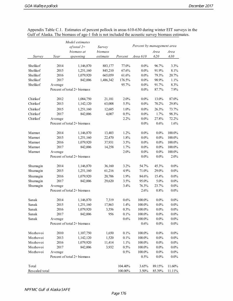
Appendix Table C.1. Estimates of percent pollock in areas 610-630 during winter EIT surveys in the Gulf of Alaska. The biomass of age-1 fish is not included the acoustic survey biomass estimates.

Percent Area 610Area 620

Area 630

Shelikof 2014 1,146,870 883,177 77.0% 0.0% 96.7% 3.3%Shelikof 2015 1,251,160 845,210 67.6% 0.0% 91.9% 8.1%Shelikof 2016 1,079,920 665,059 61.6% 0.0% 79.3% 20.7%Shelikof 2017 842,006 1,486,342 176.5% 0.0% 98.9% 1.1%Shelikof Average 95.7% 0.0% 91.7% 8.3%

Percent of total 2+ biomass 0.0% 87.7% 7.9%

Chirikof 2012 1,084,750 21,181 2.0% 0.0% 13.0% 87.0%Chirikof 2013 1,142,120 63,008 5.5% 0.0% 70.2% 29.8%Chirikof 2015 1,251,160 12,685 1.0% 0.0% 26.3% 73.7%Chirikof 2017 842,006 4,007 0.5% 0.0% 1.7% 98.3%Chirikof Average 2.2% 0.0% 27.8% 72.2%

Percent of total 2+ biomass 0.0% 0.6% 1.6%

Marmot 2014 1,146,870 13,403 1.2% 0.0% 0.0% 100.0%Marmot 2015 1,251,160 22,470 1.8% 0.0% 0.0% 100.0%Marmot 2016 1,079,920 37,931 3.5% 0.0% 0.0% 100.0%Marmot 2017 842,006 14,258 1.7% 0.0% 0.0% 100.0%Marmot Average 2.0% 0.0% 0.0% 100.0%

Percent of total 2+ biomass 0.0% 0.0% 2.0%

Shumagin 2014 1,146,870 36,160 3.2% 54.7% 45.3% 0.0%Shumagin 2015 1,251,160 61,216 4.9% 71.0% 29.0% 0.0%Shumagin 2016 1,079,920 20,706 1.9% 84.6% 15.4% 0.0%Shumagin 2017 842,006 29,620 3.5% 95.0% 5.0% 0.0%Shumagin Average 3.4% 76.3% 23.7% 0.0%

Percent of total 2+ biomass 2.6% 0.8% 0.0%

Sanak 2014 1,146,870 7,319 0.6% 100.0% 0.0% 0.0%Sanak 2015 1,251,160 17,863 1.4% 100.0% 0.0% 0.0%Sanak 2016 1,079,920 3,556 0.3% 100.0% 0.0% 0.0%Sanak 2017 842,006 956 0.1% 100.0% 0.0% 0.0%Sanak Average 0.6% 100.0% 0.0% 0.0%

Percent of total 2+ biomass 0.6% 0.0% 0.0%

Mozhovoi 2010 1,107,750 1,650 0.1% 100.0% 0.0% 0.0%Mozhovoi 2013 1,142,120 1,520 0.1% 100.0% 0.0% 0.0%Mozhovoi 2016 1,079,920 11,414 1.1% 100.0% 0.0% 0.0%Mozhovoi 2017 842,006 3,932 0.5% 100.0% 0.0% 0.0%Mozhovoi Average 0.5% 100.0% 0.0% 0.0%

Percent of total 2+ biomass 0.5% 0.0% 0.0%

Total 104.40% 3.65% 89.15% 11.60%Rescaled total 100.00% 3.50% 85.39% 11.11%

Survey Year

Percent by management areaModel estimates

of total 2+ biomass at spawning

Survey biomass estimate

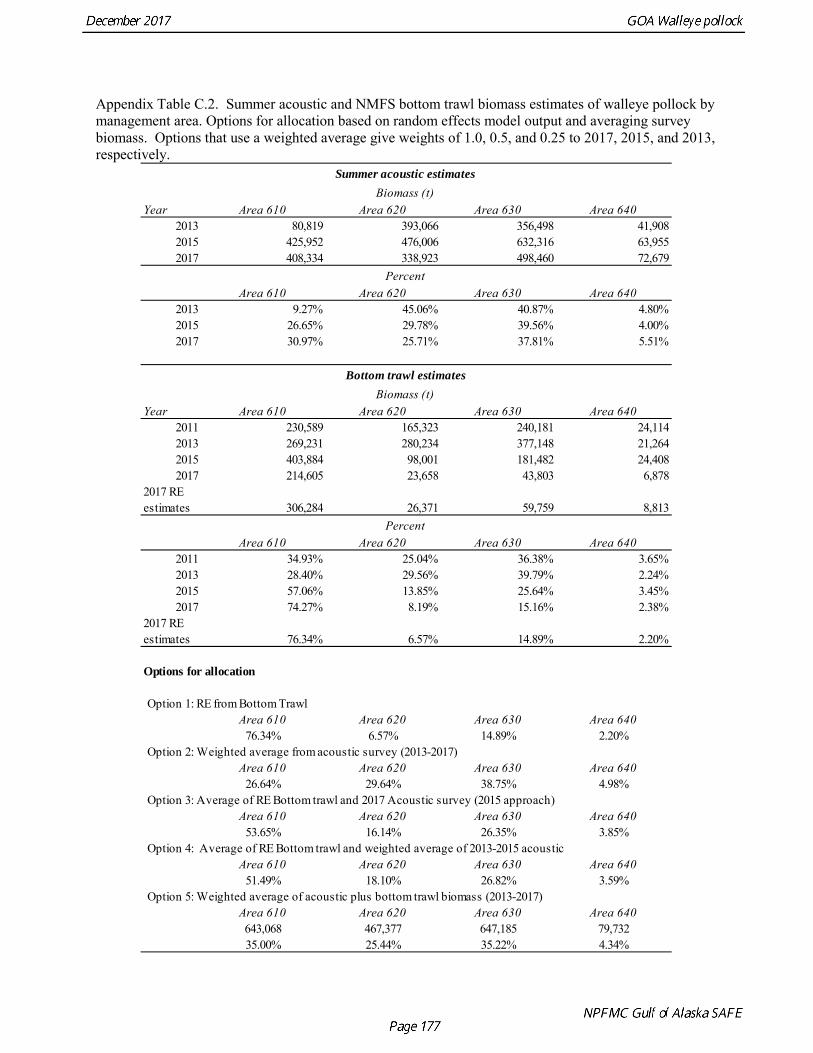
Appendix Table C.2. Summer acoustic and NMFS bottom trawl biomass estimates of walleye pollock by management area. Options for allocation based on random effects model output and averaging survey biomass. Options that use a weighted average give weights of 1.0, 0.5, and 0.25 to 2017, 2015, and 2013, respectively.

Year Area 610 Area 620 Area 630 Area 6402013 80,819 393,066 356,498 41,9082015 425,952 476,006 632,316 63,9552017 408,334 338,923 498,460 72,679

Area 610 Area 620 Area 630 Area 6402013 9.27% 45.06% 40.87% 4.80%2015 26.65% 29.78% 39.56% 4.00%2017 30.97% 25.71% 37.81% 5.51%

Year Area 610 Area 620 Area 630 Area 6402011 230,589 165,323 240,181 24,1142013 269,231 280,234 377,148 21,2642015 403,884 98,001 181,482 24,4082017 214,605 23,658 43,803 6,878

2017 RE estimates 306,284 26,371 59,759 8,813

Area 610 Area 620 Area 630 Area 6402011 34.93% 25.04% 36.38% 3.65%2013 28.40% 29.56% 39.79% 2.24%2015 57.06% 13.85% 25.64% 3.45%2017 74.27% 8.19% 15.16% 2.38%

2017 RE estimates 76.34% 6.57% 14.89% 2.20%

Options for allocation

Option 1: RE from Bottom TrawlArea 610 Area 620 Area 630 Area 640

76.34% 6.57% 14.89% 2.20%Option 2: Weighted average from acoustic survey (2013-2017)

Area 610 Area 620 Area 630 Area 64026.64% 29.64% 38.75% 4.98%

Option 3: Average of RE Bottom trawl and 2017 Acoustic survey (2015 approach)Area 610 Area 620 Area 630 Area 640

53.65% 16.14% 26.35% 3.85%Option 4: Average of RE Bottom trawl and weighted average of 2013-2015 acoustic

Area 610 Area 620 Area 630 Area 64051.49% 18.10% 26.82% 3.59%

Option 5: Weighted average of acoustic plus bottom trawl biomass (2013-2017)Area 610 Area 620 Area 630 Area 640643,068 467,377 647,185 79,73235.00% 25.44% 35.22% 4.34%

Percent

Summer acoustic estimates

Bottom trawl estimates

Biomass (t)

Biomass (t)

Percent

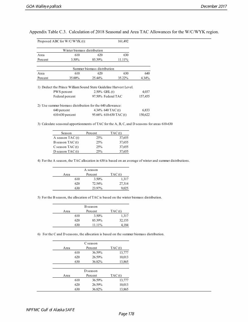
Appendix Table C.3. Calculation of 2018 Seasonal and Area TAC Allowances for the W/C/WYK region.

Proposed ABC for W/C/WYK (t): 161,492

Area 610 620 630Percent 3.50% 85.39% 11.11%

Area 610 620 630 640Percent 35.00% 25.44% 35.22% 4.34%

1) Deduct the Prince William Sound State Guideline Harvest Level.PWS percent 2.50% GHL (t) 4,037Federal percent 97.50% Federal TAC 157,455

2) Use summer biomass distribution for the 640 allowance:640 percent 4.34% 640 TAC (t) 6,833610-630 percent 95.66% 610-630 TAC (t) 150,622

3) Calculate seasonal apportionments of TAC for the A, B, C, and D seasons for areas 610-630

Season Percent TAC (t)A season TAC (t) 25% 37,655B season TAC (t) 25% 37,655C season TAC (t) 25% 37,655D season TAC (t) 25% 37,655

4) For the A season, the TAC allocation in 630 is based on an average of winter and summer distributions.

Area Percent TAC (t)610 3.50% 1,317620 72.54% 27,314630 23.97% 9,025

5) For the B season, the allocation of TAC is based on the winter biomass distribution.

Area Percent TAC (t)610 3.50% 1,317620 85.39% 32,155630 11.11% 4,184

6) For the C and D seasons, the allocation is based on the summer biomass distribution.

Area Percent TAC (t)610 36.59% 13,777620 26.59% 10,013630 36.82% 13,865

Area Percent TAC (t)610 36.59% 13,777620 26.59% 10,013630 36.82% 13,865

D season

Summer biomass distribution

Winter biomass distribution

A season

B season

C season

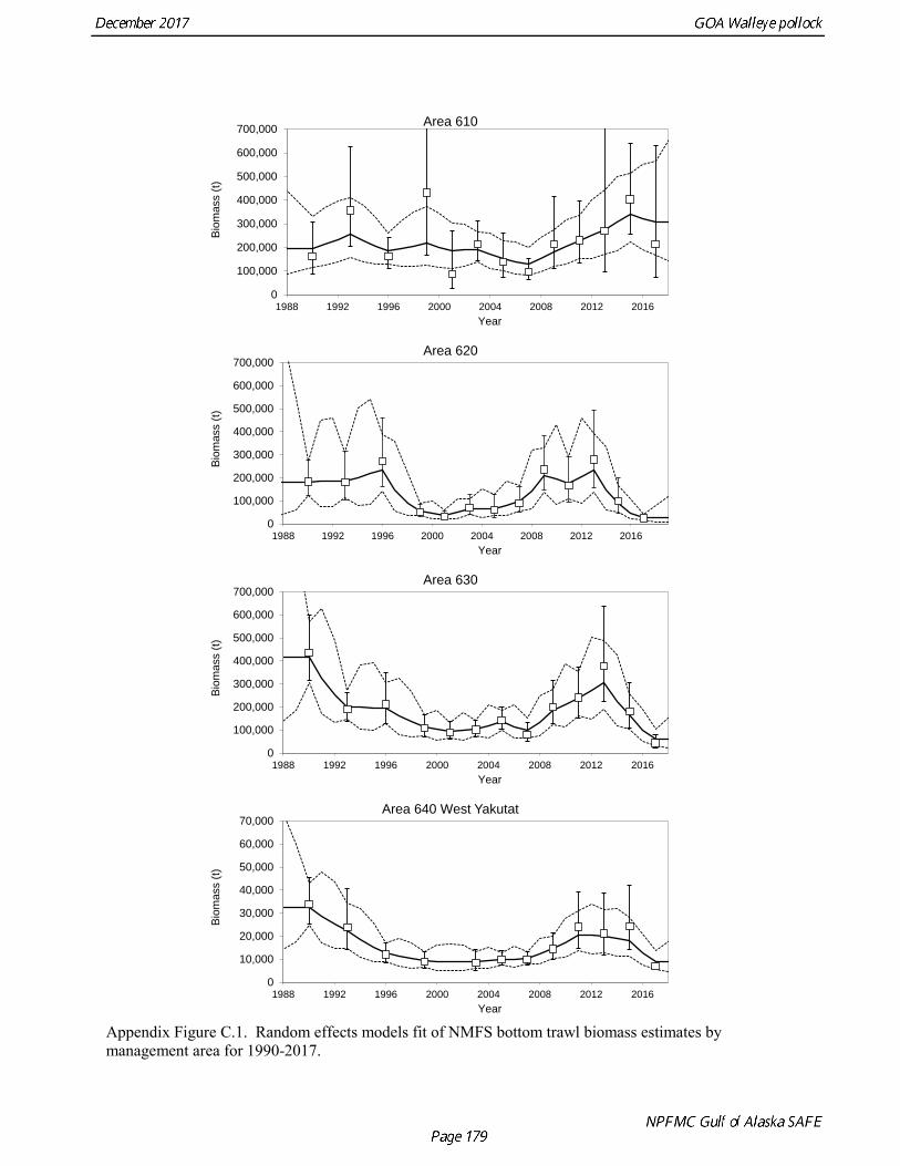
Appendix Figure C.1. Random effects models fit of NMFS bottom trawl biomass estimates by management area for 1990-2017.

0

100,000

200,000

300,000

400,000

500,000

600,000

700,000

1988 1992 1996 2000 2004 2008 2012 2016

Biom

ass

(t)

Year

Area 610

0

100,000

200,000

300,000

400,000

500,000

600,000

700,000

1988 1992 1996 2000 2004 2008 2012 2016

Biom

ass

(t)

Year

Area 620

0

100,000

200,000

300,000

400,000

500,000

600,000

700,000

1988 1992 1996 2000 2004 2008 2012 2016

Biom

ass

(t)

Year

Area 630

0

10,000

20,000

30,000

40,000

50,000

60,000

70,000

1988 1992 1996 2000 2004 2008 2012 2016

Biom

ass

(t)

Year

Area 640 West Yakutat

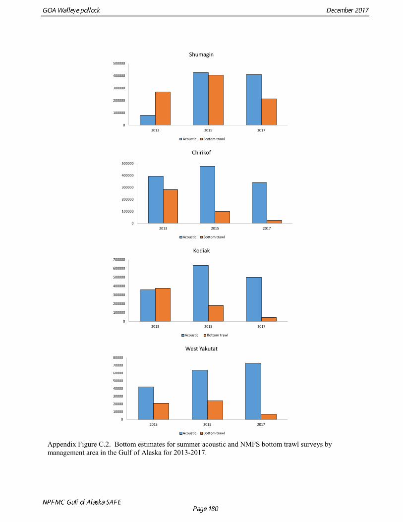
Appendix Figure C.2. Bottom estimates for summer acoustic and NMFS bottom trawl surveys by management area in the Gulf of Alaska for 2013-2017.

0

100000

200000

300000

400000

500000

2013 2015 2017

Shumagin

Acoustic Bottom trawl

0

100000

200000

300000

400000

500000

2013 2015 2017

Chirikof

Acoustic Bottom trawl

0

100000

200000

300000

400000

500000

600000

700000

2013 2015 2017

Kodiak

Acoustic Bottom trawl

0

10000

20000

30000

40000

50000

60000

70000

80000

2013 2015 2017

West Yakutat

Acoustic Bottom trawl

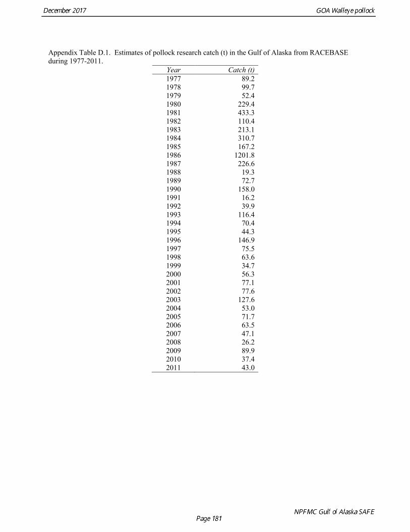
Appendix Table D.1. Estimates of pollock research catch (t) in the Gulf of Alaska from RACEBASE during 1977-2011.

Year Catch (t) 1977 89.2 1978 99.7 1979 52.4 1980 229.4 1981 433.3 1982 110.4 1983 213.1 1984 310.7 1985 167.2 1986 1201.8 1987 226.6 1988 19.3 1989 72.7 1990 158.0 1991 16.2 1992 39.9 1993 116.4 1994 70.4 1995 44.3 1996 146.9 1997 75.5 1998 63.6 1999 34.7 2000 56.3 2001 77.1 2002 77.6 2003 127.6 2004 53.0 2005 71.7 2006 63.5 2007 47.1 2008 26.2 2009 89.9 2010 37.4 2011 43.0

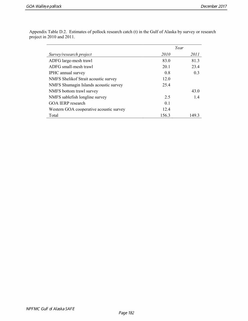
Appendix Table D.2. Estimates of pollock research catch (t) in the Gulf of Alaska by survey or research project in 2010 and 2011.

Year Survey/research project 2010 2011 ADFG large-mesh trawl 83.0 81.3 ADFG small-mesh trawl 20.1 23.4 IPHC annual survey 0.8 0.3 NMFS Shelikof Strait acoustic survey 12.0 NMFS Shumagin Islands acoustic survey 25.4 NMFS bottom trawl survey 43.0 NMFS sablefish longline survey 2.5 1.4 GOA IERP research 0.1 Western GOA cooperative acoustic survey 12.4 Total 156.3 149.3