Associate Professor Camelia OPREAN, PhD E-mail: … - Oprean Camelia...Camelia Oprean, Cristina Tanasescu, Vasile Bratian _____ balanced markets. Fama (1970) have operationalized this

Associate Professor Camelia OPREAN, PhD

E-mail: [email protected]

Associate Professor Cristina TĂNĂSESCU, PhD

Associate Professor Vasile BRĂTIAN, PhD

University Lucian Blaga of Sibiu

ARE THE CAPITAL MARKETS EFFICIENT? A FRACTAL

MARKET THEORY APPROACH

Abstract: Efficient Market Hypothesis (EMH) has attracted a considerable

number of studies in empirical finance, particularly in determining the market

efficiency of the capital markets. Conflicting and inconclusive outcomes have been

generated by various existing studies in EMH. The purpose of the fractal market

theory approach of this paper is to investigate whether the selected capital markets

abide by a particular evolution pattern or the random walk hypothesis. In this

paper, the Hurst exponent calculated by the R/S analysis is our measure of long

range dependence in the series. As a result, we may note that the Brazilian

financial market is the closest one to the random walk hypothesis, a characteristic

of efficient market hypotheses. Nevertheless, the Estonian, Chinese and Romanian

financial markets are the furthest ones from the random walk premise, as they

observe the fractal Brownian motion.

Keywords: market efficiency, fractal, Hurst exponent, R/S analysis.

JEL Classification: C5, G1

1. Introduction: market efficiency in the light of the classical EMH

theories

Considerations concerning the efficiency of financial markets lay under

two theories: random walk and the theory of efficient markets. The first theory,

random walk, is the theory of random movement of the financial assets. Elaborated

during the 6th decade of the 20th century, it supports the idea that the future

movement of an asset is independent from past movements of assets on a market.

In an informational efficient market, price movements are unpredictable, because

they encompass the information and expectations of all market participants.

The second theory, which refers to the hypothesis of efficient markets, was

established in the early 60s and assumes that asset markets process with great

sensitivity the economic intelligence which they receive and react quickly to adjust

the course of financial assets. The theory of efficient markets justifies the need of

Camelia Oprean, Cristina Tanasescu, Vasile Bratian

________________________________________________________________

balanced markets. Fama (1970) have operationalized this hypothesis. In his famous

study, which will definitively mark the theory of efficient markets, Efficient

Capital Markets: A Review of Theory and Empirical Work, written by Fama in

1970, he gives the following definition: “A market in which prices always reflect

the available information is called an efficient market”. In this paper, he realizes a

synthesis of previous research concerning the predictability of capital markets, the

notions of fair game and random walk becoming well formulated.

The theory and models regarding capital market operation have initially

developed from the assumption that these represent efficient markets. Rational

agents quickly assimilate any kind of information that proves relevant to asset

pricing and their output and subsequently adjusts the price in accordance with this

information. By way of explanation, agents do not benefit from different

comparative advantages in the process of information acquisition. To sum up, the

efficient market hypothesis refers mainly to three fundamental and highly

controversial concepts, as we have mentioned in the previous chapters: efficient

markets, random trajectories, rational agents.

The prevailing opinion before 1970s was that the processes of evolution are

deterministic and predictable, whereas nowadays these processes are considered to

be rather stochastic and unpredictable, and even chaotic in most situations.

Financial markets represent a potential application of chaos theory in the field of

economics. The rationale for applying chaos theory to finance is that markets are

non-linear dynamic systems, so that the exclusive employment of statistical models

for the analysis of random walk standard data might lead to wrong or irrelevant

results.

Special attention has been given to the role of chaos in the field of finance

especially due to the multitude of information and the interest in identifying

predictable models. Tests have also shown that the market pricing of assets, though

unpredictable, will evince a particular trend. The capital market is commonly

acknowledged as a self-similar system, in the sense that its components are either

similar or even identical to the whole. Another type of self-similar system used in

mathematics is the fractal (the shape of the resulting structure is the same

irrespective of the scale of representation). The based on nonlinear dynamics thus

comes into being. Recent studies, particularly after 1990, have focused mainly on

developing new theory-based models, borrowed from other disciplines. Some of

these models rely on the fractal theory indicating that the seemingly random

evolution of the trend may be further decomposed in several similar evolution

periods so that the initial series enables modeling. The application of fractal

methods – Fractal Market Hypothesis (FMH) [8], [9] – allows us to explore the

chaotic nature of time series [10]. This theory is a rendering of efficient markets

where the focus is placed on market stability however, instead of market

efficiency. Thus, it takes into account the everyday market randomness as well as

market anomalies.

Are the Capital Markets Efficient? A Fractal Market Theory Approach

_______________________________________________________________

The paper is structured as follows. Section 2 describes the methodology

used in view of attaining the goal of this paper, the methods we used for the Hurst

exponent estimation. In Section 3, we describe the data and Section 4 covers the

empirical results and discusses the implications whether the selected markets are

subject to a specific evolution pattern or the random walk hypothesis. Section 5

concludes.

2. Methodology

2.1. The R/S fractal analysis method – rescaled range analysis

This method, applicable to the study of financial markets, relies on the

concept of the Hurst exponent. It was introduced by English hydrologist H.E. Hurst

in 1951, based on Einstein’s contributions regarding Brownian motion of physical

particles, to deal with the problem of reservoir control near Nile River Dam. Hurst

(1965) proved that the dynamics of many natural phenomena is given by a

randomly changed law. If the data series were perfectly random then these value

series would increase simultaneously with the square-root of time enhancement

(the √𝑇 rule). Hurst introduced the non-dimensional ratio, dividing the data series

to the standard deviation of observations to the average, in view of enabling

comparison of data selected at different time moments. The result was a

redimensioning of the scale hence the method is also called the R/S rescaled range

analysis. R/S analysis in economy was introduced by Mandelbrot (1972), who

argued that this methodology was superior to the autocorrelation, the variance

analysis and to the spectral analysis.

In this paper, the Hurst exponent calculated by the R/S analysis is our

measure of long range dependence in the series. The R/S method (range / standard

deviation) requires an initial dynamic series, standing for the evolution of a natural

phenomenon or process.

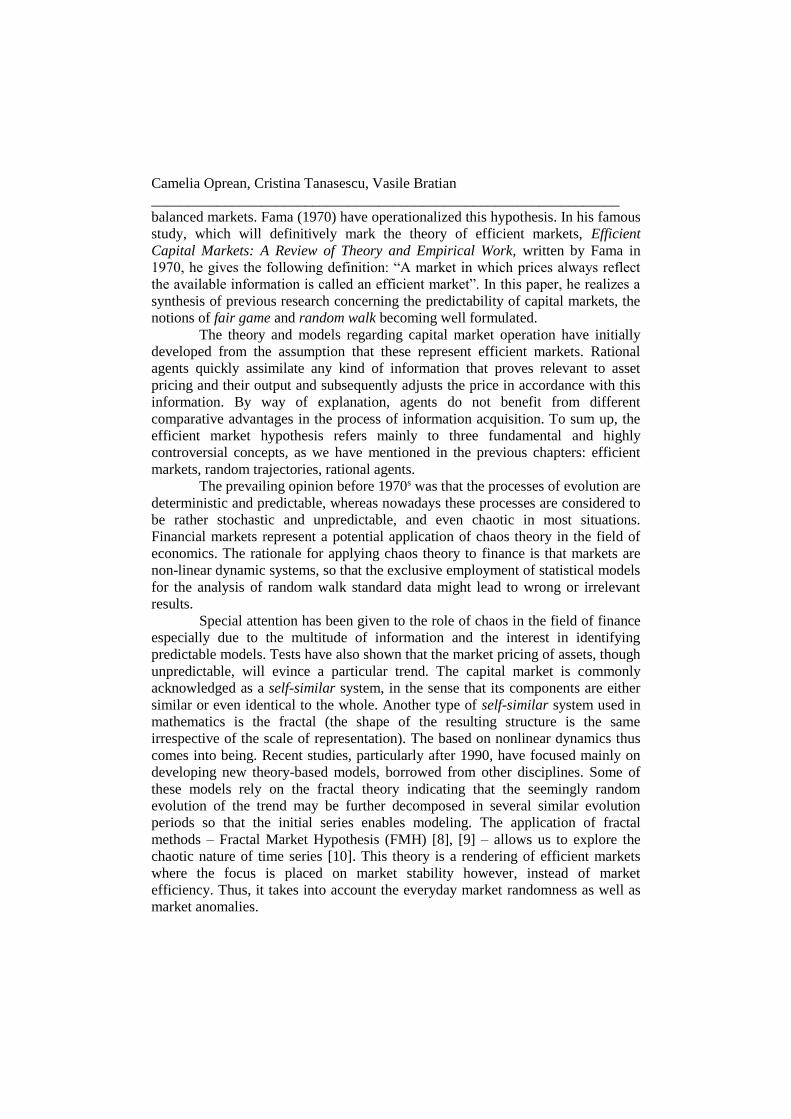
Let Pt be the price of a stock on a time t and rt be the logarithmic return

denoted by the first difference of logarithmic values of daily prices [7]:

)log()log()log( 1 tttt PPPdr (1)

As financial time series display high degree of non-stationarity, it is a

common practice to work with first differenced series than with the original series.

Therefore in the first step, we reduce non-stationarity by converting the original

series to a returns series taking logarithm returns from successive values of the

series.

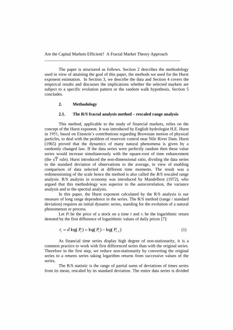
The R/S statistic is the range of partial sums of deviations of times series

from its mean, rescaled by its standard deviation. The entire data series is divided


________________________________________________________________

into several contiguous sub-periods each having n-observations and define each

sub-period as Ia, a = 1, 2, …, k, so 𝑘 ∙ 𝑛 = 𝑁. For each sub-period, the average

value of the sub-period is determined. Starting from this assumption, we may

determine the following dimension (considering that the series is divided into a

sub-periods of n range):

n

i

anian rrX1

,, )( (2)

where Xn,a represents the cumulative deviation for each Ia sub-period; ri represents

the i component of the dynamic series; rn,a represents the ri value average on every

Ia sub-period.

The range (R) of the cumulative trend adjusted return series for each sub-

period Ia is measured by taking differences of maximum and minimum values of

Xn,a:

)()( ,,, ananan XMinXMaxR (3)

Hurst divided the R value to the standard deviation of initial observations

for each Ia sub-interval, in view of comparing various dynamic series, for instance:

n

rr

S

n

i

ani

an

1

2

,

,

)(

(4)

For every Ia sub-interval, the ratio given below is further determined:

n

rr

XMinXMaxSR

n

i

ani

anan

an

1

2

,

,,

,

)(

)()()/( (5)

As there are many contiguous sub-periods, the average R/S value of full

series is calculated by averageing R/S values of all individual sub-periods:

k

a

ann SRk

SR1

,)/(1

)/( (6)


_______________________________________________________________

The n length is increased and the procedure is repeated until n = (N-1)/2.

Hurst noticed that this ratio increases as the number of observations in the

initial data series enhances. If the data series were perfectly random, then the ratio

would increase proportionally with the square root of the number of observations

√𝑁. Brownian motion is the primary model for a random walk process. Einstein

(1908) found the distance a particle covers increases with respect to time according

to the following relation:

5.0TR (7)

where R is the distance covered by the particle in time T (see [8], [9]).

We can use equation (7) only if the time series we are considering is

independent of increasing values of T. To take into account the fact that economic

time series systems are not independent with respect to time, Hurst (1965) found a

more general form of equation (7). In order to measure the R/S ratio enhancement

in dependence on the phenomenon observation time, Hurst employed the following

relation:

H

n ncSR )/( (8)

where c is a proportionality constant and H represents the Hurst exponent.

Afterwards, the value of Hurst exponent (H) is established by means of

regression:

)log()log()log()/log( nHcncSR H

n (9)

2.2. Hurst exponent analysis

This paper computes the Hurst statistics by means of the aforementioned

R/S method (apart from the classical estimation, a different methodology shall also

be used (i.e. [3]) in order to calculate the Hurst exponent) to identify the existence

of long-term linear dependence in the stock market volatility. In this framework,

we adopt 16 fixed-sized windows of n observations to compute the extent of

inefficiency (n = 10, 20, 30, 40, 60, 80, 100, 120, 200, 240, 300, 400, 500, 600,

800, 1200).

a. Long-term correlation analysis

In the case of a time series, whenever the Hurst exponent is other than 0.5,

correspondingly the breakeven point has no common distribution, hence any time

series observation is no longer independent. The recent observations are attached to


________________________________________________________________

the “memory” of previous observations, also called long-term memory character.

Mandelbrot introduced a coefficient for measuring the correlation (between

increases occurring at future moments to increases at previous time), Cn, with the

following significance in correlation with the Hurst exponent:

12 )12( H

nC (10)

where Cn represents the correlation coefficient evinced throughout the time

range subject to analysis.

The relation between fractal dimension D (used to identify whether the

system is at random) and Hurst exponent is: D = 1/H [5]. The random walk has a

fractal dimension of 1/0.5 = 2. Therefore, it fully covers the entire space. If we also

take into consideration this relation, three different values of Hurst exponent can

tell three different types of time series:

- the Hurst exponent equals 0.5 the series is no longer correlated, and the events

are perfectly random (C = 0, D = 1.5). It is standard Brownian motion. In

other words, the present cannot influence the future. The event-related

probability density function may be the common one or any other probability

distribution. Fractional Brownian motion is a well-known stochastic process

where the second order moments of the increments scale as:

H

iiii tttYtYE2

1

2

1)()( (11)

with H ϵ [0, 1]. The Brownian motion is then the particular case where

H = ½.

- the correlation coefficient is less than zero, D > 1.5 (provided that 0 ≤ H <

0.5), therefore the series is negatively correlated. This type of dynamic series is

the antipersistent fractal Brownian motion (a characteristic of self-adjustment

systems), so that an increase in the series term will most likely entail its

decrease, at the next moment in time. The intensity of antipersistent behavior

depends on H`s closeness to zero. If H = 0, then C = -0.5 which makes, under

these circumstances, the series highly volatile and subject to frequent changes.

Given that the system covers a smaller distance compared to the random

movement, its evolution changes its sign more often than a random process;

- the Cn correlation coefficient is greater than zero, D < 1.5 (whenever 0.5 < H ≤

1), therefore the series is positively correlated and we thus encounter a

persistent dynamics, i.e. if a value increased (decreased) previously, then very

likely it will continue increasing (decreasing). The intensity of persistent

behavior depends on the H value: whenever H tends to 1, then C tends to 1,

too. Persistent dynamic series are fractal, since they are actualy functional

Brownian motions with a correlation among events in time.


_______________________________________________________________

To sum up, for any t1 and t2 moments, if:

- H = ½ we have a normal Brownian motion;

- otherwise, there is a fractal Brownian motion.

The difference between the two motions is that the fractal Brownian

motion evinces correlations on an infinitely large scale.

b. Statistic Vn

Statistic Vn was originally used to test the stability of R/S analysis method

[11]. Peters expanded it to accurately measure the critical point n and average cycle

length:

n

SRV n

n

)/( (12)

For the time series of independent stochastic process, the curve of Vn

concerning log(n) is a straight line. If the sequence possesses a state persistence,

i.e. when 0.5 < H < 1, Vn concerning log(n) is upward raked; if the sequence has an

inverse state persistence, i.e. when 0 < H < 0.5, Vn concerning log(n) is sloped

downward.

c. Significance Test and the expectation value of H

The greatest fault of the early-period R/S analysis is the lack of

significance test. As to random walk hypothesis, H = 0.5 is a gradual process.

When the study sample is limited, the value of H of random sequence always

deviates from 0.5. At this time the expectation value of H can be derived from the

following formula (Peters, 1994):

1

15.0

15.0)/(

n

i

ni

in

nn

nSRE

(13)

From the following regression analysis we can get the value of E(H):

)log()()log()/(log nHEcSRE n (14)

R/Sn is the random variable of normal distribution, thus E(H) also follows

the normal distribution, expectation variance Var(H)n = 1/N, N is the total sample

capacity. The null hypothesis of this significance test is H0: H = E(H) that is the


________________________________________________________________

Gaussian process of random walk; the alternative hypothesis H1: H ≠ E(H) that

sequence is biased random walk and has persistence and memory effect. The

statistic t of hypothesis test is:

N

HEHt

/1

)( (15)

The loss of accuracy of R/S analysis in some specific cases (problems to

study long range dependence when series is not large enough) has been remarked

by some authors ([3], [9], [12] and others).

Following Weron (2002), once E(R/S)n is calculated, the Hurst exponent H

will be 0.5 plus the slope of (R/S)n − E(R/S)n. However, if we calculate this

modified R/S analysis in this way, results show a Hurst exponent, for some random

series, with values higher than 1, which makes no sense. For this reason, we have

followed a different procedure [3] that lies in adding other step to the classical R/S

analysis which consist in calculating:

2/log)/(log/loglog nSRESRH nnn (16)

Then find H by linear regression on:

nHcHn logloglog (17)

3. Data

The data of this survey represent daily stock market quotes of the most

traded indices in the eight emergent capital market countries, four UE countries

and the four BRIC countries (BET for Romania, OMX Tallin for Estonia, PX for

the Czech Republic, BUX for Hungary, BOVESPA for Brazil, SENSEX for India,

RTSI for Russia, and the Shanghai Composite Index for China). The indices are

selected as they can best reflect and exhaustively capture all events on a market.

Data has been mainly collected from stock exchange own websites,

showing the indices transaction. We have collected daily values over a ten-year

time span, between October 2002 – May 2014, in order to reach conclusions based

on thorough and accurate data; the time span thus enabled a proper modeling of the

phenomena occurring on the respective capital markets. The data sample consists

of an average of 2500 daily values of each index price separately.

4. Results

The aim of the tests we are going to perform is to identify whether the selected

markets are subject to a specific evolution pattern or the random walk hypothesis.


_______________________________________________________________

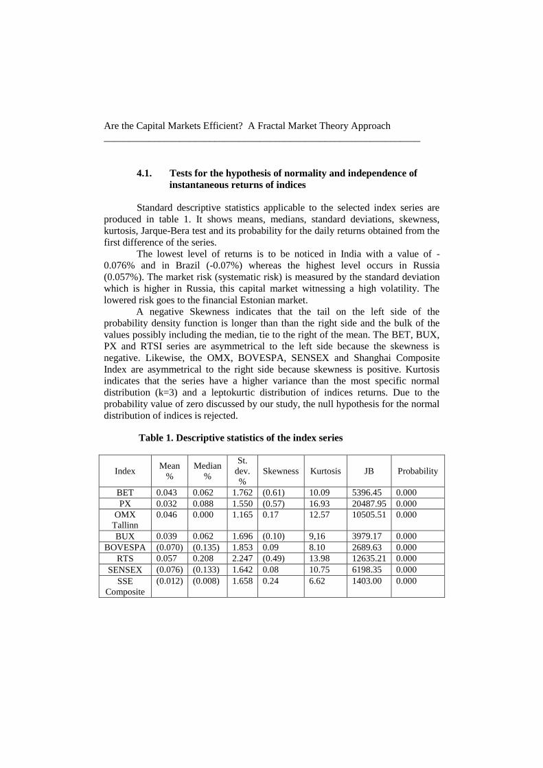
4.1. Tests for the hypothesis of normality and independence of

instantaneous returns of indices

Standard descriptive statistics applicable to the selected index series are

produced in table 1. It shows means, medians, standard deviations, skewness,

kurtosis, Jarque-Bera test and its probability for the daily returns obtained from the

first difference of the series.

The lowest level of returns is to be noticed in India with a value of -

0.076% and in Brazil (-0.07%) whereas the highest level occurs in Russia

(0.057%). The market risk (systematic risk) is measured by the standard deviation

which is higher in Russia, this capital market witnessing a high volatility. The

lowered risk goes to the financial Estonian market.

A negative Skewness indicates that the tail on the left side of the

probability density function is longer than than the right side and the bulk of the

values possibly including the median, tie to the right of the mean. The BET, BUX,

PX and RTSI series are asymmetrical to the left side because the skewness is

negative. Likewise, the OMX, BOVESPA, SENSEX and Shanghai Composite

Index are asymmetrical to the right side because skewness is positive. Kurtosis

indicates that the series have a higher variance than the most specific normal

distribution (k=3) and a leptokurtic distribution of indices returns. Due to the

probability value of zero discussed by our study, the null hypothesis for the normal

distribution of indices is rejected.

Table 1. Descriptive statistics of the index series

Index Mean

%

Median

%

St.

dev.

%

Skewness Kurtosis JB Probability

BET 0.043 0.062 1.762 (0.61) 10.09 5396.45 0.000

PX 0.032 0.088 1.550 (0.57) 16.93 20487.95 0.000

OMX

Tallinn

0.046 0.000 1.165 0.17 12.57 10505.51 0.000

BUX 0.039 0.062 1.696 (0.10) 9,16 3979.17 0.000

BOVESPA (0.070) (0.135) 1.853 0.09 8.10 2689.63 0.000

RTS 0.057 0.208 2.247 (0.49) 13.98 12635.21 0.000

SENSEX (0.076) (0.133) 1.642 0.08 10.75 6198.35 0.000

SSE

Composite

(0.012) (0.008) 1.658 0.24 6.62 1403.00 0.000


________________________________________________________________

Also, we cannot conclude that the series of returns have normal

distributions using the Jarque Bera test. Most markets exhibit deviations (volatility)

from normality. Due to the fact that returns are correlated and do not have a normal

distribution, we reject the hypothesis that supports the idea that these time series

are yielding a random model, therefore, we question the existence of a weaker

form of informational efficiency for the eight emergent capital markets.

Emergent markets are defined by a non-linear behavior of information in

terms of stock prices. Consequently, we applied the BDS independence test in

order to determine the time dependence throughout a given chronological

sequence. The assumption that a system represents a nonlinear process is one of the

cahos theory premises that has got the attention of most economists. The BDS test

developed by Brock, Dechert, Scheinkman and Le Baron (1996) is arguably the

most popular test for nonlinearity. It does not directly test chaos (which would be

impossible) but only nonlinearity. If evidence of nonlinearity should be found in

time series, this shows for at least a short period of time, that predictions may be

improved by alternating from a linear to a nonlinear strategy.

Moreover, it can be used as a mis-specification test when applied to the

residuals from a fitted model. Evidence of nonlinear dependence of returns may

create doubts on the informational efficiency of financial markets. In particular,

when applied to the residuals from a fitted linear time series model, the BDS test

can be used to detect remaining dependence and the presence of omitted nonlinear

structure.

The null hypothesis (H0) of an identical and independent distribution is

tested. If the null hypothesis H0 is accepted, the original linear model cannot be

rejected (accepted). If H0 is rejected, the fitted linear model is mis-specified and in

this sense, it can also be regarded as a test for non-linearity. If the BDS value is

statistically higher than 1.96 (2.58) then H0 is rejected at a 5% significance level.

However, the BDS test has power against a wide range of linear and

nonlinear alternatives and it is applied in most cases to the residuals of a linear

model (we applied it on the residuals of the AR(1) model or GARCH type). This

step is regarded as a type of pre-filtering of data, making possible the observation

of any potential determinism of the analysed data, except for the one described by

a linear or a GARCH type process. Brock et al. (1997) recommends an ε distance

threshold between 1 and 3 halves of a standard deviation for an increased testing

power. The analysis is performed for the embedding dimensions ε/σ = 1 and ε/σ = 2

(and is presented below in the table 2):


_______________________________________________________________

Table 2. BDS statistical test

BDS statistic, ε/σ = 1

dimension BET BUX OMX PX BOVESPA RTS SENSEX SHANGHAI

2 0.037297 0.016510 0.039452 0.026454 0.006932 0.023988 0.022707 0.009618

3 0.063036 0.027507 0.067514 0.048955 0.014309 0.045526 0.040908 0.021200

4 0.075473 0.032011 0.081820 0.059431 0.018055 0.054914 0.049526 0.026310

5 0.077386 0.031927 0.085954 0.062799 0.018738 0.056800 0.051592 0.026408

The results confirm the rejection of a null hypothesis H0 and of an identical

and independent distribution, nonlinearity of all series of indices is therefore

considered to be checked.

4.2. Statically analysis of Hurst exponent

Based on the aforementioned method, we have obtained the following

results for the indicators of the eight emergent financial markets, presented in the

table 3, which gives a classification of countries subject to analysis on the basis of

the Hurst exponent value:

Table 3. Indices classification according to the value of Hurst exponent

Classification Index Hurst

exponent

Correlation

coefficient C

Fractal

Dimension D

8 BOVESPA (Brazil) 0.583565 0.49854769 1.713605

5 RTS (Russia) 0.676366 0.59810921 1.478489

7 SENSEX (India) 0.647230 0.56615826 1.545046

2 SHANGHAI_C_I (China) 0.709749 0.63551954 1.408949

3 BET (Romania) 0.709547 0.63529056 1.40935

6 BUX (Hungary) 0.662280 0.58258172 1.509935

4 PX (Czech Republic) 0.679205 0.60125714 1.47231

1 OMX Tallinn (Estonia) 0.791595 0.73098713 1.263272

Subsequent to the calculation of the Hurst exponent for the analysed stock-

exchange indices, we may notice, as an overall trend, that all rate series are

persistent, since the value of the Hurst exponent ranges between 0.5 and 1.


________________________________________________________________

Therefore, the value of correlation coefficients is also more than zero, so that the

series are positively correlated. Hence, if a term in the sequence has increased, it

will most probably increase, at the next moment in time. All stock quote sequences

undergo a fractal Brownian motion, different than the common random walk. The

intensity of the persistent behavior is dependent on the H`s closeness to one. Given

this correlation of events, the probability that two events should succeed each other

is no longer 0.5. The Hurst exponent represents the probability that two similar

events should occur consecutively. This is a fractal series, since each occurrence of

an event is no longer equally probable, unlike perfectly random dynamic series.

Further to the classification performed in keeping with the Hurst exponent

and presented in the graph above, we may note that the Brazilian financial market

is the closest one to the random walk hypothesis, a characteristic of efficient

market hypotheses. Nevertheless, the Estonian, Chinese and Romanian financial

markets are the furthest ones from the random walk premise, as they observe the

fractal Brownian motion.

The R/S analysis shows the fractal distribution of short-term market

performance distribution, which requires a self-similar structure. This hypothesis

explains the structure by means of multiple investment horizons of investors. That

is, the presence of investors who choose to invest on different time spans at any

time scale will make the distribution probability time-scale independent, which can

definitely be called a characteristic of a fractal distribution.

Whenever, the application of the Hurst exponent to the time sequences

testifies that the series are not independent, hence they do not meet the randomness

criterion, we may conclude that each term of the dynamic sequence includes a

long-term memory of past events, instead of a short-term memory from one term to

another. Recent events have had a greater impact upon current observations,

whereas previous events tend to have a less significant impact, however they still

retain a residual influence [6].

4.3. Statistic Vn

Furthermore, V-statistic is also used for enhancing signals or bumps in the

graph entailed by its cyclic behavior. When the graphic shape of Vn changes, it

produces the sudden mutation, and the long-term memory also disappears.

Therefore, we can see directly the influence time boundary of the value of time

series at a certain moment on the future values with the relation curve of Vn

concerning log(n). For the eight indices included in the analysis, the evolution of

Vn statistic and log R/S according to log(n) shows that in all situations, the time

series is defined by a state persistence (when 0.5 < H < 1), because the sequence Vn

concerning log(n) is upward raked. In the case of independent stochastic process,

the curve of Vn concerning log(n) would be a straight line [11].


_______________________________________________________________

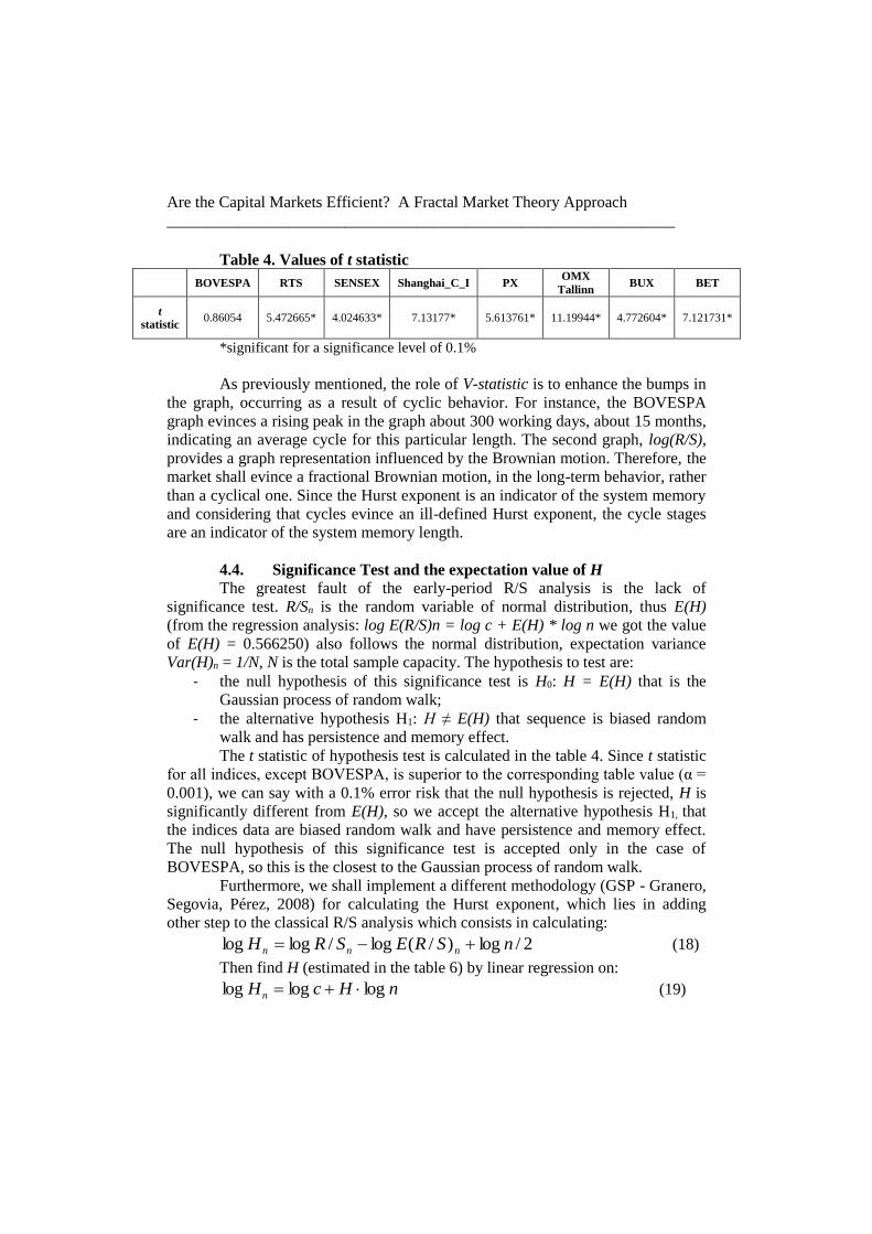
Table 4. Values of t statistic

BOVESPA RTS SENSEX Shanghai_C_I PX OMX

Tallinn BUX BET

t

statistic 0.86054 5.472665* 4.024633* 7.13177* 5.613761* 11.19944* 4.772604* 7.121731*

*significant for a significance level of 0.1%

As previously mentioned, the role of V-statistic is to enhance the bumps in

the graph, occurring as a result of cyclic behavior. For instance, the BOVESPA

graph evinces a rising peak in the graph about 300 working days, about 15 months,

indicating an average cycle for this particular length. The second graph, log(R/S),

provides a graph representation influenced by the Brownian motion. Therefore, the

market shall evince a fractional Brownian motion, in the long-term behavior, rather

than a cyclical one. Since the Hurst exponent is an indicator of the system memory

and considering that cycles evince an ill-defined Hurst exponent, the cycle stages

are an indicator of the system memory length.

4.4. Significance Test and the expectation value of H

The greatest fault of the early-period R/S analysis is the lack of

significance test. R/Sn is the random variable of normal distribution, thus E(H)

(from the regression analysis: log E(R/S)n = log c + E(H) * log n we got the value

of E(H) = 0.566250) also follows the normal distribution, expectation variance

Var(H)n = 1/N, N is the total sample capacity. The hypothesis to test are:

- the null hypothesis of this significance test is H0: H = E(H) that is the

Gaussian process of random walk;

- the alternative hypothesis H1: H ≠ E(H) that sequence is biased random

walk and has persistence and memory effect.

The t statistic of hypothesis test is calculated in the table 4. Since t statistic

for all indices, except BOVESPA, is superior to the corresponding table value (α =

0.001), we can say with a 0.1% error risk that the null hypothesis is rejected, H is

significantly different from E(H), so we accept the alternative hypothesis H1, that

the indices data are biased random walk and have persistence and memory effect.

The null hypothesis of this significance test is accepted only in the case of

BOVESPA, so this is the closest to the Gaussian process of random walk.

Furthermore, we shall implement a different methodology (GSP - Granero,

Segovia, Pérez, 2008) for calculating the Hurst exponent, which lies in adding

other step to the classical R/S analysis which consists in calculating:

2/log)/(log/loglog nSRESRH nnn (18)

Then find H (estimated in the table 6) by linear regression on:

nHcHn logloglog (19)


________________________________________________________________

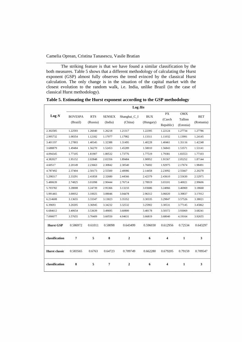
The striking feature is that we have found a similar classification by the

both measures. Table 5 shows that a different methodology of calculating the Hurst

exponent (GSP) almost fully observes the trend evinced by the classical Hurst

calculation. The only change is in the situation of the capital market with the

closest evolution to the random walk, i.e. India, unlike Brazil (in the case of

classical Hurst methodology).

Table 5. Estimating the Hurst exponent according to the GSP methodology

Log N

Log Hn

BOVESPA

(Brazil)

RTS

(Russia)

SENSEX

(India)

Shanghai_C_I

(China)

BUX

(Hungary)

PX

(Czech

Republic)

OMX

Tallinn

(Estonia)

BET

(Romania)

2.302585 1.22593 1.26040 1.26218 1.21317 1.22395 1.22124 1.27734 1.27786

2.995732 1.08354 1.12182 1.17077 1.17982 1.13311 1.11032 1.13991 1.24145

3.401197 1.27803 1.40545 1.32388 1.31495 1.40228 1.40461 1.35116 1.42248

3.688879 1.49484 1.56270 1.52453 1.45289 1.58010 1.56843 1.53571 1.53141

4.094345 1.77105 1.81907 1.80532 1.73776 1.77519 1.79381 1.83553 1.77103

4.382027 1.95152 2.02848 2.02356 1.89484 1.90952 1.91567 2.05252 1.87144

4.60517 2.20149 2.23663 2.30842 2.30540 1.76692 1.92975 2.17674 1.98491

4.787492 2.37404 2.50173 2.55500 2.40086 2.14458 2.23092 2.55667 2.20278

5.298317 2.33291 2.41858 2.32680 2.44566 2.42379 2.43610 2.55630 2.52975

5.480639 2.74825 3.01098 2.90444 2.76714 2.78919 3.03101 3.40021 2.99606

5.703782 3.28008 3.24739 2.95366 3.13233 3.03686 3.24966 3.46969 3.18668

5.991465 3.00052 3.10025 3.08046 3.04478 2.96312 3.06020 3.39837 3.17012

6.214608 3.13655 3.33347 3.13023 3.35352 3.30335 3.29847 3.57526 3.38021

6.39693 3.20205 3.36945 3.34232 3.32532 3.25902 3.30531 3.77145 3.45862

6.684612 3.40654 3.53639 3.49695 3.60800 3.48178 3.50372 3.93069 3.68241

7.090077 3.57655 3.70409 3.60550 4.04631 3.66819 3.68040 4.19164 3.92655

Hurst GSP 0.586972 0.61011 0.58098 0.643499 0.596030 0.612956 0.72534 0.643297

classification 7 5 8 2 6 4 1 3

Hurst classic 0.583565 0.6763 0.64723 0.709749 0.662280 0.679205 0.79159 0.709547

classification 8 5 7 2 6 4 1 3


_______________________________________________________________

5. Conclusions

An application of normality and independence tests on the logarithmic

profitability of the index series, shows that almost all markets evince significant

deviations from normality. The time series composed of stock indices also evinces

nonlinearity. The existence of a poor informational efficiency for the eight

emergent capital markets is highly questionable.

Subsequent to the classical calculation of the Hurst exponent for the stock

indices subject to analysis, we have noticed that all trends are persistent, since the

value of the Hurst exponent ranges between 0.5 and 1. Therefore, the value of

correlation coefficients is above zero, so that the series are positively correlated.

According to the Hurst exponent value, the Brazilian financial market is closest to

the random walk hypothesis, specific to efficient market hypothesis. On the other

hand, the financial market from Estonia, China and Romania prove to be the

furthest from the random walk hypothesis, characterized by the highest degree of

fractal Brownian motion.

A different methodology of calculating the Hurst exponent (GSP) almost

fully observes the trend shown by the classical Hurst calculation, where only case

of the capital market whose evolution is closest to the random walk (i.e. India,

unlike Brazil – as in the case of the classical Hurst methodology) is slightly

changed.

To sum up, the tests performed in this paper indicate that the yields of

these emergent stock markets is a persistent series submitting to fractal

distribution.

REFERENCES

[1] Brock, W. A., Dechert, W. D., Scheinkman, J. A., Lebaron, B. (1996), A

Test for Independence Based on the Correlation Dimension; Econometric

Reviews, 15, 197-235;

[2]Fama, E. (1970), Efficient Capital Markets: A Review of Theory and

Empirical Work; Journal of Finance, 25(2), 383-417;

[3]Granero, M.A. S., Segovia, J.E. T., Perez, J. G. (2008), Some Comments on

Hurst Exponent and the Long Memory Processes on Capital Markets; Physica A,

387, 5543–5551;

[4]Hurst, H. E., Black, R. P., Simaika, Y. M. (1965), Long-Term Storage: An

Experimental Study ;Constable Publishing House;


________________________________________________________________

[5]Mandelbrot, B. (1972), Statistical Methodology for Nonperiodic Cycles from

Covariance to R/S Analysis ; Annals of Economic and Social Measurement, 1,

259–290;

[6]Maracine, V., Scarlat, E. (2002), Aplicații ale teoriei haosului în economie;

Revista Informatică Economică, 1(21), 110-115

[7]Mundnich, K., Orchard, M.E., Silva, J.F., Parada, P. (2013), Volatility

Estimation of Financial Returns Using Risk-Sensitive Particle Filters ; Studies in

Informatics and Control, 22(3), 297-306

[8]Peters, E. (1994), Fractal Market Analysis; Wiley, New York;

[9]Peters, E. (1996), Chaos and Order in the Capital Markets; John Wiley and

Sons;

[10]Steeb, W.H., Andrieu, E.C. (2005), Ljapunov Exponents, Hyperchaos and

Hurst Exponent . Verlag der Zeitschrift fur Naturforschung, Tubingen, 60a,

252 – 254;

[11]Wang, Y., Wang, J., Guo, Y., Wu, X., Wang, J. (2011), FMH and Its

Application in Chinese Stock Market ; CESM, Part II, CCIS 176, Springer-Verlag

Berlin Heidelberg, 349–355;

[12]Weron, R. (2002), Measuring Long-range Dependence in Electricity Prices;

H. Takayasu, Empirical Science of Financial Fluctuations, Springer-Verlag,

Tokyo, 110-119.

Documents

Associate Professor Camelia OPREAN, PhD E-mail: … - Oprean Camelia...Camelia Oprean, Cristina Tanasescu, Vasile Bratian _____ balanced markets. Fama (1970) have operationalized this