Associate Professor Mirela Camelia BABA, PhD - Dinca Gheorghita, Dinca...Gheorghita Dinca, Camelia Baba, Sorin Dinca, Bardhyl Dauti, Fitim Deari _____ 140 by their companies), as well

Economic Computation and Economic Cybernetics Studies and Research, Issue 4/2017, Vol. 51

________________________________________________________________________________

139

Associate Professor Gheorghita DINCA, PhD

E-mail: [email protected]

Associate Professor Mirela Camelia BABA, PhD


Asociate Professor Marius Sorin DINCA, PhD (Coresponding author)


Faculty of Economic Sciences and Business Administration

Transilvania University of Brasov

Assistant Professor Bardhyl DAUTI, PhD

Faculty of Economics, University of Tetovo


Assistant Professor Fitim DEARI, PhD

Faculty of Business and Economics

South East European University, Tetovo


INSOLVENCY RISK PREDICTION USING THE LOGIT AND

LOGISTIC MODELS: SOME EVIDENCES FROM ROMANIA

Abstract. The authors have studied insolvency situation from Romania in

the aftermath of the 2008 financial crisis, using 5 years of financial statements data for 70 Romanian companies from different economic sectors, which all

entered insolvency in 2013. We have designed a model for predicting insolvency

risk which can be used by any interested party, since the data for the model are readily available on the site of Romanian Fiscal Administration Agency. The

model uses five financial ratios, whose dynamics is analyzed for at least three

years. To test the model we have used a logit and logistic model, which validated

the significant influence of total assets efficiency and accounts receivable conversion period upon insolvency risk. As such, managers and investors can

follow especially the evolution of these two measures and make the best credit and

investing decisions concerning analyzed companies. Keywords: Romanian insolvencies; prediction model; economic and

financial measures; logit and logistic models.

JEL Classification: L10, M10

Introduction

In Romania recent years have accounted for a large number of companies

which became insolvent, turning the issue of estimating this risk into a priority, both for managers (which need tools to predict and control the potential risks faced

mailto:[email protected]





Gheorghita Dinca, Camelia Baba, Sorin Dinca, Bardhyl Dauti, Fitim Deari

________________________________________________________________

140

by their companies), as well as for trading partners (who need such information to

design proper commercial credit and investment policies in relation with the analyzed company).

Most insolvency risk studies were based on multivariate, discriminant

analysis, whose results were used to generate score functions to estimate

companies’ state of health. However, many insolvency risks’ predicting models present a range of shortcomings which makes them not applicable to all the

companies requiring insolvency risks’ forecast at a certain moment in time. On the

one hand, many of these models were aimed for companies listed on the stock exchange and on the other hand, even if such models are not intended for listed

companies, they are based on accounting information not accessible to external

users, thereby significantly reducing the range of models’ potential users. In the same time, score functions’ based models have, due to their invariable coefficients,

an applicability confined to the economic-geographic area for which they were

created. As such, the coefficients determined by authors according to the

economic-geographic features of the industry and country for which they were designed, require caution while using them, even in case of similar geographic and

economic conditions, yet at different moments in time.

Unlike managers, which have at their disposal detailed information about their companies’ economic and financial situation, the trading partners of unlisted

Romanian companies cannot access other information than excerpts from these

companies’financial statements data, published by the National Agency for Fiscal

Administration (NAFA) on its website. Moreover, this information is processed and summarized and thus insufficient to be used in established prediction models

to determine insolvency risk.

We propose a model for insolvency risk’s diagnosis which can be used by any party (especially external users) interested in the health of a Romanian

company, based on public and official information originating from its annual

financial statements, whether listed or not on the Stock Exchange and regardless of its size. The model is primarily intended for trading partners, who can thus

establish the economic and financial health of their potential partners and identify

those facing insolvency risk. Based on this information they can further decide

about the opportunity of initiating or continuing their business relations. The reminder of the paper is organized as follows: section two approaches

literature review; section three presents Romania 2013’s insolvency situation;

section four approaches the model to estimate insolvency risk and data analysis; section five is dedicated to model testing, whilst conclusions are presented in

section six.

1. Literature review Starting with the 2008 global economic crisis, insolvency became a

concept subject to numerous studies and debates. Many researchers from Romania

and abroad analyzed and debated the delicate/thorny issue of economic entities’

insolvency.

Insolvency Risk Prediction Using the Logit and Logistic Models: Some Evidences

from Romania

_________________________________________________________________

141

European cross-border insolvency rules are established by EC’s Regulation 1346/2000 (Insolvency Regulation) regarding insolvency proceedings,

applicable starting May the 31-th 2002.

In Romania insolvency is regulated and defined by art. 3, paragraph 1, of Law 85/2006 as "the state of the debtor's heritage characterized by lack of funds

available for payment of due debts". From a legal perspective, the causes leading

to the dissolution of a company are those provided by Law 31/1990 on trading

companies, republished, and are divided into common causes for all types of companies and specific causes for equity companies, respectively for partnerships.

There are a variety of models for predicting bankruptcy. In the literature

we can find several types of insolvency risk prediction models, respectively MDA (Multiple Discriminate Analysis) models, logical regression models, neural

networks’ models or mixed logit ones.The scoring method has become very

popular over time due to its use of statistical methods for financial situation’s analysis, starting from a set of ratios. The most common scoring method’s models

are Altman’s, Springate’s, Koh’s model, Conan-Holder’s, and the one of Banque

de France.Scientific models for bankruptcy prediction based on financial indicators

have been developed for the first time in the USA in the 1960’s, by Altman (1968) and Beaver (1966). The first wide range model of bankruptcy risk analysis,

commonly known as the Z score function, belonged to Altman, who published it

firstly in 1968. Altman’s model is based on the discriminate analysis, creating classification/prediction models which include data and observation in certain a

priori determined classes. Altman et al. (1977) built another model known as Zeta

model, analyzing 53 bankrupt and 58 viable companies during 1969-1975. Ohlson (1980) and Platt & Platt (1990) conducted the first studies using

the logit model for predicting companies’ state of insolvency. Zmijewski (1984)

advanced the probit model to predict companies’ bankruptcy risk. The econometric

models are based on logit and probit models in particular. Default-prediction literature acknowledged logit model as being the most used technique to determine

default’s probability. The results of Ohlson’s model have shown that firm size,

financial structure, performance and current liquidity were the main determinants of companies’ insolvency. Shumway (2001) proposed a hazard model for

predicting bankruptcy firms, defined as a multi-period logit model. One main

feature of the hazard model is that explanatory variables vary over several time

periods, resulting in more efficient estimators. In his work he studied 300 bankrupt firms from the 1962 to 1992 period. Decision trees method for predicting

insolvencies (the advantages of using CHAID classification trees compared to a

neural network model) was used by Zheng and Yanhui (2007). Bankruptcy is due to economic and financial factors, negligence, fraud, as

well as other factors. Economic factors, causing 37.1% of bankruptcies, relate

particularly to industry weakness and unfavorable location. Financial factors, holding the highest percentage, of 47.3%, include too much debt and insufficient

capital. The analysis showed that most financial factors relate to huge errors,


________________________________________________________________

142

misjudgments, and management’s reduced capacity of financial prediction

(Brigham and Ehrhardt, 2007). There are many causes of business failure, some related to managers’

experience and skills, while other causes are due to general economic conditions,

the recession. As such, Burksaitiene and Mazintiene (2011) aim to provide

managers with information about possible causes and consequences of failure in their companies. Other authors tried to demonstrate Altman’s model effectiveness

in predicting retail companies’ financial difficulties (Hayes et al., 2010). Kiyak and

Labanauskaitė (2012) conducted a comparative analysis for several models of bankruptcy prediction and reliability, concluding that linear discrimination model

most accurately reflected the financial position of the company (for companies in

Lithuania). Pereira and Machado-Santos studied the way the established predictive models can be applied in various fields or types of economies in different

countries, analyzing Portugal’s textile companies insolvency (2007); Zeytinoglu

and Akar (2013) attempted to identify bankruptcy risk for Istanbul Stock Exchange

listed companies; Gharaibeh et al. (2013) analyzed insolvency of Jordan Stock Exchange listed companies (the applicability of prediction models for emerging

economies - the case of Jordan); Szeverin and László (2014) analyzed bankruptcy

prediction models’ efficiency for small and medium size entities in Hungary. Recent studies (Karas and Režňáková, 2014) examined how bankruptcy prediction

model’s efficiency is influenced by the choice of a certain method, especially the

linear discriminant analysis method.

In Romania studies developing scoring functions for bankruptcy’s risk analysis occurred much later compared to research conducted worldwide. Anghel

(2000) conducted a comprehensive bankruptcy risk study, creating a score function

based on a sample of 276 companies. Generally, the idea of limiting the findings and applicability of a score function only to the economic sector for which it was

built is widely accepted, even if it turned out that some models have a high degree

of applicability. This is because the models recognized worldwide were built under a stable economy, while the Romanian economy is still under a long process of

consolidation.

Studies concerning bankruptcy risk’s estimation, aimed to discriminate

bankrupt companies from the ones with a good financial situation, based on financial ratios, have been conducted by Vintilă and Toroapă (2012), which

developed a bankruptcy predicting econometric model. Korol and Korodi (2011)

aimed to demonstrate Fuzzy logic’s effectiveness in predicting bankruptcy risk and proposed an econometric model in this regard.To highlight the financial strength

and ability to meet obligations of Romanian companies listed on Bucharest Stock

Exchange, Armeanu et al. (2012) have performed an Altman scoring function on a sample of 60 companies, using seven financial indicators, representative for

company’s activity: total assets, net turnover, operating result, net cash flow from

operating activities, net profit, debt – total liabilities and average market

capitalization.


from Romania

_________________________________________________________________

143

2. 2013 Romania’s Insolvencies Situation The situation of Romanian companies which entered into a state of

insolvency in 2013 has been studied so far mainly from the points of view of its

evolution, of insolvencies distribution’s fluctuation from a geographical point of view or according to field of activity, many studies in this area belonging to Coface

Romania. According to information published by Romania’s National Trade

Register Office (NTRO) after a slight improvement (a decrease of 9.41%) in 2011

compared to 2010, in 2012 followed a strong growth of 36.42% in the number of recorded insolvencies. The increase of insolvencies’ number continued in the year

2013, exceeding by 10.37% the ones recorded in 2012.

Most insolvencies were recorded in Bucharest city, representing 12.70% of 2013’s total number of insolvencies in Romania. Bucharest was followed by Bihor,

Galati, Brasov and Constanta counties, which recorded between 4.08% and 6.17%

of all insolvencies recorded in Romania in 2013. These four counties, together with Bucharest accounted for a third of all 2013 Romanian insolvencies, with remaining

Romanian counties recording a less significant number of insolvencies, holding

each between 0.73% and 3.80% of total amount. The territorial distribution showed

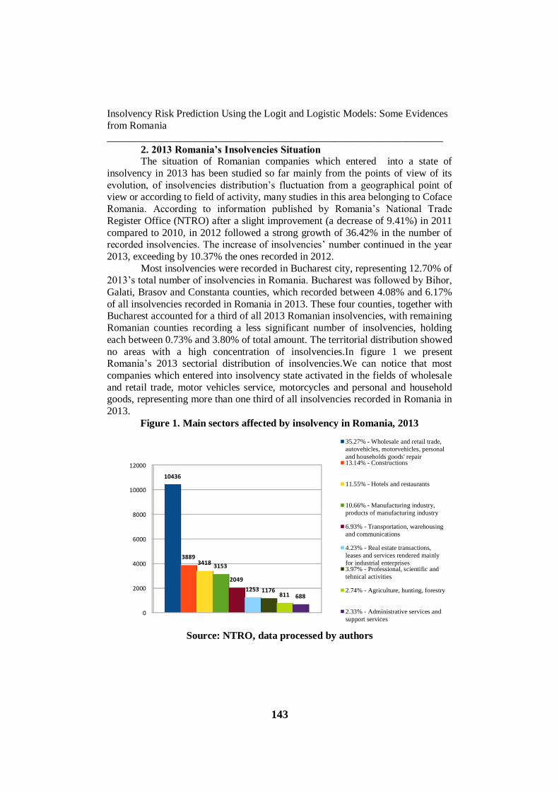
no areas with a high concentration of insolvencies.In figure 1 we present Romania’s 2013 sectorial distribution of insolvencies.We can notice that most

companies which entered into insolvency state activated in the fields of wholesale

and retail trade, motor vehicles service, motorcycles and personal and household goods, representing more than one third of all insolvencies recorded in Romania in

2013.

Figure 1. Main sectors affected by insolvency in Romania, 2013

Source: NTRO, data processed by authors

0

2000

4000

6000

8000

10000

12000

10436

38893418 3153

2049

1253 1176811 688

35.27% - Wholesale and retail trade,

autovehicles, motorvehicles, personal

and households goods' repair13.14% - Constructions

11.55% - Hotels and restaurants

10.66% - Manufacturing industry,

products of manufacturing industry

6.93% - Transportation, warehousing

and communications

4.23% - Real estate transactions,

leases and services rendered mainly

for industrial enterprises3.97% - Professional, scientific and

tehnical activities

2.74% - Agriculture, hunting, forestry

2.33% - Administrative services and

support services


________________________________________________________________

144

3. The Model to Estimate Insolvency Risk and Data Analysis The purpose of our paper is to develop an insolvency risk’s diagnosis

model, usable by any party interested in an economic entity’s health. The model

can be applied by users with access to detailed financial statements, as well as by

people with access only to summary information published by financial authorities. Unlike models based on score functions, influenced by invariable coefficients, our

model is based solely on financial ratios fluctuations’ analysis over time. In this

way, the model can be applied to any company, regardless of the economic, geographical and temporal conditions. This study was conducted under the

conditions of eliminating any outside influences, specific for the industry,

geographic area, size of companies or the general health of the economy, relying exclusively on economic and financial information derived from the annual

financial statements published by the commercial companies.

The model, designed for an early warning of financial difficulty of

economic entities, is based on a set of five measures, respectively general solvency, patrimonial solvency, accounts receivable conversion period, assets’

liquidity and assets’ efficiency ratio. The selection of financial indicators was

conditioned by the availability of financial data provided by Romania’s Administration of Public Finance.

To identify insolvency symptoms’ occurrence, we have analyzed 350

financial statements from the last 5 years prior to insolvency of 70 Romanian

economic entities. For all the 70 economic entities the insolvency proceedings opened in 2013. Our model is designed to identify the elements which help assess

the probability a company enters a state of insolvency, respectively the elements

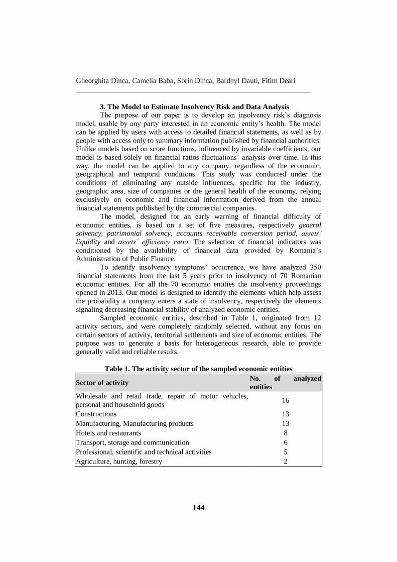
signaling decreasing financial stability of analyzed economic entities. Sampled economic entities, described in Table 1, originated from 12

activity sectors, and were completely randomly selected, without any focus on

certain sectors of activity, territorial settlements and size of economic entities. The purpose was to generate a basis for heterogeneous research, able to provide

generally valid and reliable results.

Table 1. The activity sector of the sampled economic entities

Sector of activity No. of analyzed

entities

Wholesale and retail trade, repair of motor vehicles,

personal and household goods 16

Constructions 13

Manufacturing, Manufacturing products 13

Hotels and restaurants 8

Transport, storage and communication 6

Professional, scientific and technical activities 5

Agriculture, hunting, forestry 2


from Romania

_________________________________________________________________

145

Activities of administrative services and activities of support services

2

Other activities of collective, social and personal services 2

Information and communication 1

Education 1

Water supply; sanitation, waste management 1

TOTAL 70

Source: Authors’ decision

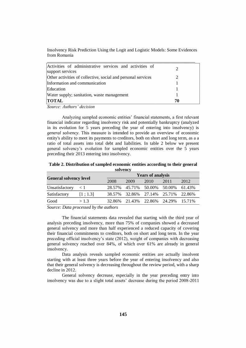
Analyzing sampled economic entities’ financial statements, a first relevant financial indicator regarding insolvency risk and potentially bankruptcy (analyzed

in its evolution for 5 years preceding the year of entering into insolvency) is

general solvency. This measure is intended to provide an overview of economic entity's ability to meet its payments to creditors, both on short and long term, as a a

ratio of total assets into total debt and liabilities. In table 2 below we present

general solvency’s evolution for sampled economic entities over the 5 years

preceding their 2013 entering into insolvency.

Table 2. Distribution of sampled economic entities according to their general

solvency

General solvency level Years of analysis

2008 2009 2010 2011 2012

Unsatisfactory < 1 28.57% 45.71% 50.00% 50.00% 61.43%

Satisfactory [1 ; 1.3] 38.57% 32.86% 27.14% 25.71% 22.86%

Good > 1.3 32.86% 21.43% 22.86% 24.29% 15.71%

Source: Data processed by the authors

The financial statements data revealed that starting with the third year of

analysis preceding insolvency, more than 75% of companies showed a decreased

general solvency and more than half experienced a reduced capacity of covering their financial commitments to creditors, both on short and long term. In the year

preceding official insolvency’s state (2012), weight of companies with decreasing

general solvency reached over 84%, of which over 61% are already in general insolvency.

Data analysis reveals sampled economic entities are actually insolvent

starting with at least three years before the year of entering insolvency and also that their general solvency is decreasing throughout the review period, with a sharp

decline in 2012.

General solvency decrease, especially in the year preceding entry into

insolvency was due to a slight total assets’ decrease during the period 2008-2011


________________________________________________________________

146

and an abrupt decline in 2012, and to a relatively steady growth of total debt

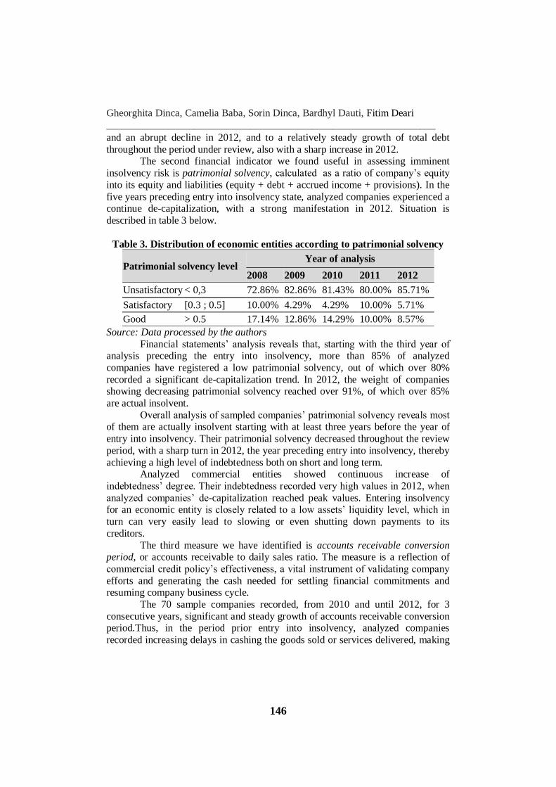
throughout the period under review, also with a sharp increase in 2012. The second financial indicator we found useful in assessing imminent

insolvency risk is patrimonial solvency, calculated as a ratio of company’s equity

into its equity and liabilities (equity + debt + accrued income + provisions). In the

five years preceding entry into insolvency state, analyzed companies experienced a continue de-capitalization, with a strong manifestation in 2012. Situation is

described in table 3 below.

Table 3. Distribution of economic entities according to patrimonial solvency

Patrimonial solvency level Year of analysis

2008 2009 2010 2011 2012

Unsatisfactory < 0,3 72.86% 82.86% 81.43% 80.00% 85.71%

Satisfactory [0.3 ; 0.5] 10.00% 4.29% 4.29% 10.00% 5.71%

Good > 0.5 17.14% 12.86% 14.29% 10.00% 8.57%


Financial statements’ analysis reveals that, starting with the third year of analysis preceding the entry into insolvency, more than 85% of analyzed

companies have registered a low patrimonial solvency, out of which over 80%

recorded a significant de-capitalization trend. In 2012, the weight of companies showing decreasing patrimonial solvency reached over 91%, of which over 85%

are actual insolvent.

Overall analysis of sampled companies’ patrimonial solvency reveals most of them are actually insolvent starting with at least three years before the year of

entry into insolvency. Their patrimonial solvency decreased throughout the review

period, with a sharp turn in 2012, the year preceding entry into insolvency, thereby

achieving a high level of indebtedness both on short and long term. Analyzed commercial entities showed continuous increase of

indebtedness’ degree. Their indebtedness recorded very high values in 2012, when

analyzed companies’ de-capitalization reached peak values. Entering insolvency for an economic entity is closely related to a low assets’ liquidity level, which in

turn can very easily lead to slowing or even shutting down payments to its

creditors.

The third measure we have identified is accounts receivable conversion period, or accounts receivable to daily sales ratio. The measure is a reflection of

commercial credit policy’s effectiveness, a vital instrument of validating company

efforts and generating the cash needed for settling financial commitments and resuming company business cycle.

The 70 sample companies recorded, from 2010 and until 2012, for 3

consecutive years, significant and steady growth of accounts receivable conversion period.Thus, in the period prior entry into insolvency, analyzed companies

recorded increasing delays in cashing the goods sold or services delivered, making


from Romania

_________________________________________________________________

147

it more difficult to repay existing debt and being subsequently compelled to call in additional debt to continue.

The progressive increase of account receivable conversion period was due

to a slight yet steady turnover’s decline during the five years analyzed and to a sudden rise of accounts receivable in the last two years’ prior entry into

insolvency, namely 2011 and 2012; these two elements combined generated a

sharp increase of accounts receivable conversion period.

Our model’s fourth measure is assets’ liquidity, or the ratio of current assets into total assets, designed to provide information regarding company’s

operational flexibility and its capacity to serve commercial and financial

commitments. Analyzed companies recorded, starting with the third year before entry into

insolvency, increases of asset liquidity, which could be a positive sign of their

ability to service debts and therefore to keep away from insolvency risk. However, looking further into the evolution of current assets’ components,

we find that asset liquidity’s increase was unhealthy. Two components of this

assets liquidity’s increase, respectively inventories and cash, fluctuated, yet

remained somehow stable during the 2008-2011 period. This was followed by inventories and cash decreases in 2012. Thus, their cumulated evolution for the

entire period is negative and opposite of growth tendency registered by assets’

liquidity. The only current assets’ component which recorded a sharp increase, especially in 2012, is accounts receivable, whose 2012 growth has been strong

enough to more than compensate cash and inventories’ decreases and determine

assets liquidity’s increase.However, correlating this with the evolution of accounts receivable conversion period, we find out that, although assets’ liquidity grew in

the period preceding the entry into insolvency, analyzed companies actually had

increasing difficulties in covering their debts as they come due.

The fifth measure we have considered is assets’ efficiency, the ratio between company turnover and total assets employed to generate respective sales.

Overall, the 70 companies analyzed have recorded a slight decrease in total assets’

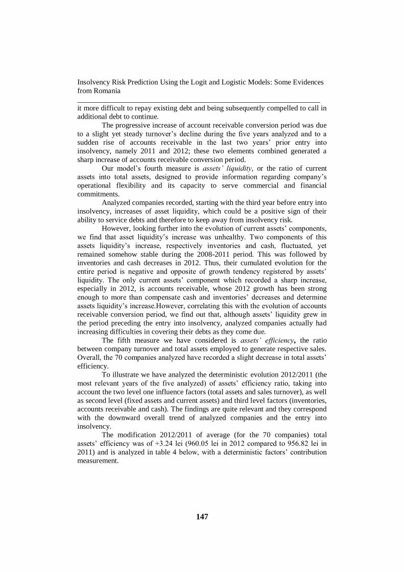
efficiency. To illustrate we have analyzed the deterministic evolution 2012/2011 (the

most relevant years of the five analyzed) of assets’ efficiency ratio, taking into

account the two level one influence factors (total assets and sales turnover), as well

as second level (fixed assets and current assets) and third level factors (inventories, accounts receivable and cash). The findings are quite relevant and they correspond

with the downward overall trend of analyzed companies and the entry into

insolvency. The modification 2012/2011 of average (for the 70 companies) total

assets’ efficiency was of +3.24 lei (960.05 lei in 2012 compared to 956.82 lei in

2011) and is analyzed in table 4 below, with a deterministic factors’ contribution measurement.


________________________________________________________________

148

Table 4. Factors’ contributions to total assets’ efficiency modification

2012/2011

Source: authors’ calculation

Where: TAE – total assets’ efficiency, the ratio of sales to total assets;

Index of TA 12/11 – index of total assets 2012/2011;

𝐼𝑛𝑑𝑒𝑥 𝑜𝑓 𝑠𝑎𝑙𝑒𝑠12/11– index of sales 2012/2011;

k% CA – percentage contribution of current assets tototal assets’ change 2012/2011;

k% A/R – percentage contribution of accounts receivable to total assets’ change

2012/2011; k% M – percentage contribution of cash&liquid assets to total assets’ change

2012/2011.

From table 4 we can find that total assets’ efficiency increased in 2012

compared to 2011 (a level higher by 3.23 lei for 1000 lei invested in total assets).

Measures Factors’

Contributions

1. Contribution of total assets:

𝑇𝐴𝐸11 (1

𝐼𝑛𝑑𝑒𝑥 𝑜𝑓 𝑇𝐴 12/11− 1)

+44.6411

1.1 Contribution of fixed assets:

𝑇𝐴𝐸11 (1

𝐼𝑛𝑑𝑒𝑥 𝑜𝑓 𝑇𝐴 12/11 − 𝐾%𝐶𝐴− 1)

-8.6356

1.2 Contribution of current assets:

𝑇𝐴𝐸11 (1

𝐼𝑛𝑑𝑒𝑥 𝑜𝑓 𝑇𝐴 12/11−

1

𝐼𝑛𝑑𝑒𝑥 𝑜𝑓 𝑇𝐴 12/11 − 𝐾%𝐶𝐴)

+53.2768

1.2.1 Contribution of inventories:

𝑇𝐴𝐸11 (1

𝐼𝑛𝑑𝑒𝑥 𝑜𝑓 𝑇𝐴 12/11 − 𝐾%𝐴/𝑅 − 𝐾%𝑀

−1

𝐼𝑛𝑑𝑒𝑥 𝑜𝑓 𝑇𝐴 12/11 − 𝐾%𝐶𝐴)

+23.1899

1.2.2 Contribution of accounts’ receivable:

𝑇𝐴𝐸11 (1

𝐼𝑛𝑑𝑒𝑥 𝑜𝑓 𝑇𝐴 12/11 − 𝐾%𝑀

−1

𝐼𝑛𝑑𝑒𝑥 𝑜𝑓 𝑇𝐴 12/11 − 𝐾%𝐴/𝑅 − 𝐾%𝑀)

-36.3151

1.2.3 Contribution of cash and short-term investments:

𝑇𝐴𝐸11 (1

𝐼𝑛𝑑𝑒𝑥 𝑜𝑓 𝑇𝐴 12/11−

1

𝐼𝑛𝑑𝑒𝑥 𝑜𝑓 𝑇𝐴 12/11 − 𝐾%𝑀)

+66.4021

2. Contribution of sales turnover:

𝑇𝐴𝐸11

1

𝐼𝑛𝑑𝑒𝑥 𝑜𝑓 𝑇𝐴 12/11(𝐼𝑛𝑑𝑒𝑥 𝑜𝑓 𝑠𝑎𝑙𝑒𝑠12/11 − 1)

-41.4028


from Romania

_________________________________________________________________

149

Nevertheless, this is not a favorable evolution, since it was due to total assets’ decrease (thereby creating an apparently positive contribution of 44.64 lei)

combined with a milder sales turnover’s decrease (with a negative contribution of -

41.4 lei). We can substantiate this by deepening total assets’ contribution analysis. As such, we can find fixed assets had a negative contribution of -8.64 lei, which

reveals that sample companies made a reduced level of investments, most likely

destined to replace depreciated fixed assets (obviously creating new fixed assets is

virtually excluded under such circumstances). Furthermore, looking into the structure of current assets we can find that

their apparently positive contribution (of +53 lei) was actually due to decreases in

inventories and cash and increases in accounts receivable. This corresponds to the perfect recipe for insolvency (lower inventories, hence lower prospects of future

sales combined with a slower recovery of accounts receivable and reduced cash

amounts). After checking and correcting data for routing checks, descriptive statistics

and means by year of selected ratios are presented in table 5 below.

Descriptive statistics shows selected companies have on average 59%

current assets and 41% noncurrent assets. On average selected companies have general solvability ratio of 1.32, respectively patrimonial solvability ratio of -1.31.

Moreover, on average, companies generated 2.6 RON of sales for each RON

invested in total assets and collected their account receivables in 98 days.

Table 5. Descriptive statistics

Variable Obs. Mean

Std.

Dev. Min Max

AL (assets liquidity) 347 0.59 0.31 0.00 1.00

GS (general solvability) 346 1.32 2.15 0.00 27.74

PS (patrimonial solvability) 347 -1.31 11.09 -200.09 1.00

TAE (total assets effic.) 346 2.60 5.94 0.00 87.57

A/R (Accts. Receivable Conv. Period) 321 98.02 129.69 0.00 781.03

Y (dependent variable) 347 0.66 0.47 0.00 1.00

Source: authors’ calculation

4. Data and methodology

4.1. Applying the model

We have applied the model for an economic entity (randomly selected) not

listed in the Bulletin of Insolvency Proceedings. Practically, entity’s insolvency

risk simulation was conducted from a trading partner’s point of view. The model implies calculating the five measures and establishing each

measure’s negative evolutions from one year to another (labeled YES if there is a

negative trend and NO otherwise). The following steps consist in checking the years in which all five measure showed negative evolutions and finally counting

the consecutive years in which all five indicators had negative evolutions. In case


________________________________________________________________

150

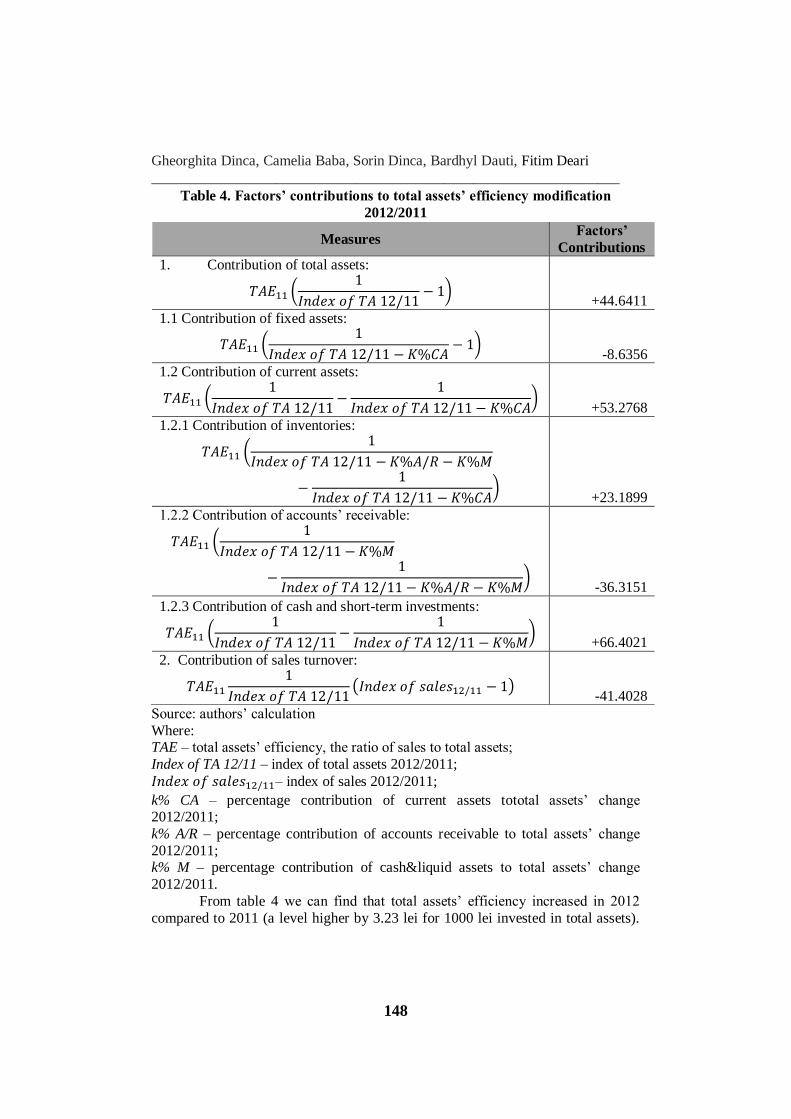
of our analyzed economic entity, there was no year in which all five measures

concurrently recorded negative evolutions, therefore it appears it presents no insolvency risk. In the same way, the test can be performed for any economic

entity, provided there is data available from the financial statements for the last

five consecutive years. Table 6 shows means of selected ratios by year. Assets

liquidity, total assets’ efficiency and A/R conversation period have positive trends, whereas general solvability, patrimonial solvability negative.

Table 6. Means by year

Year AL GS PS TAE A/R

2008 0.56 1.98 0.04 2.05 93.95

2009 0.54 1.54 -0.41 2.43 62.31

2010 0.59 1.13 -0.51 2.06 106.03

2011 0.63 1.10 -0.75 2.04 106.00

2012 0.64 0.83 -4.97 4.44 124.02

Total 0.59 1.32 -1.31 2.60 98.02


In case of analyzed economic entity, we can notice a good general and

patrimonial solvency, exceeding the 1.3, respectively the 0.5 reference thresholds for general, respectively patrimonial solvency, throughout analyzed period. These

values demonstrate economic entity's ability to pay its debts, a low degree of

indebtedness and consequently a virtually non-existent insolvency risk. These

arguments are also supported by the correlated evolutions of the measures presented in table 7.

Table 7. Indicator evolution analysis

Indicator evolution Negative evolution period

2010 2011 2012 2013

Decreasing general solvency (< 1.3) NO NO NO NO

Decreasing patrimonial solvency (<0.5) NO NO NO NO

Increasing A/R conversion period YES YES YES NO

Simultaneous increase of AL and A/R

conversion period NO NO NO NO

Declining of total assets’ efficiency YES YES YES YES

Simultaneous negative trend for all

measures NO NO NO NO


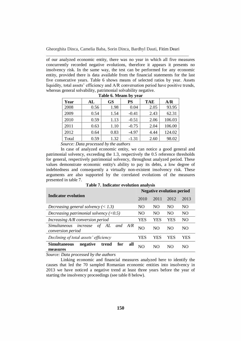
Linking economic and financial measures analyzed here to identify the causes that led the 70 sampled Romanian economic entities into insolvency in

2013 we have noticed a negative trend at least three years before the year of

starting the insolvency proceedings (see table 8 below).


from Romania

_________________________________________________________________

151

Table 8. Negative trend for at least three years

Source: Data processed by the authors An economic entity’s potential trade partner can perform the analysis of

five financial measures using at least four yearly financial statements and assessing

their evolution for at least three years. Based on this set of measures’ evolution analysis, we can estimate the level of insolvency risk presented by a potential

trading partner and the potential hazards which can affect its economic and

financial situation.

Should the five financial measures concurrently display a negative evolution, then, according to the number of years of downside trend, it is possible

to determine the level of insolvency risk. If there is just one negative evolution (a

negative evolution means that in a given year all the five measures have concurrently negative evolutions), then the company has a low risk of becoming

insolvent; if two consecutive negative evolutions occur, then the company records

an average risk of going insolvent; and if there are three consecutive years of

negative evolutions the company has an increased risk of becoming insolvent.

4.2. General form of the logit and logistic model

We rely our estimations on a Logit and Logistic model, considering a class of binary response models with the following form (Måns, 2009):

𝑃𝑟(𝑌 = 1/𝑥) = 𝐺(𝑋𝐵)

𝑃𝑟(𝑌 = 1/𝑥) = 𝐺(𝐵0 + 𝐵1𝑋1 + 𝐵2𝑋2 + ⋯ 𝐵𝑘𝑋𝑘) (1)

where G is a function taking on values strictly between 0 and 1: 0 < 𝐺(𝑧) < 1, for

all zreal numbers. The general form of the model (1) is a function of the xvector,

through the index:

𝑥𝐵 = 𝐵0 + 𝐵1𝑋1 + 𝐵2𝑋2 + ⋯ 𝐵𝑘𝑋𝑘 (2)

which is simply a scalar. The condition 0 < 𝐺(𝑥𝐵) < 1ensures estimated response

probabilities lie strictly between 0 and 1. G usually refers to the cumulative density

function (dcf), and non-linear function which is monotonally increasing in the

index z (i.e.𝑥𝐵), with:

𝑃𝑟(𝑌 = 1/𝑥) → 1, as 𝑥𝐵 → ∞

𝑃𝑟(𝑌 = 1/𝑥) → 0as 𝑥𝐵 → −∞

The most common non-linear function is the logistic distribution, yielding the logit model, as follows:

Negative trend 2009 2010 2011 2012

Decreasing general solvency (< 1.3) YES YES YES YES

Decreasing patrimonial solvency (<0.5) YES YES YES YES

Increasing A/R conversion period YES YES YES

Simultaneous AL and A/R conversion

period’s increases

YES YES YES

Decreasing total assets’ efficiency YES YES YES


________________________________________________________________

152

𝐺(𝑥𝐵) =𝑒𝑥𝑝(𝑥𝐵)

1+𝑒𝑥𝑝(𝑥𝐵)= Λ(𝑥𝐵) (3)

which has values between 0 and 1, for all values of the xBscalar term. The equation

(3) refers to thecumulative distribution function (cdf)for a logistic variable.

Since𝑃𝑟(𝑌 = 1/𝑥) in the equation (1) is categorical, we use the logit of Y as the

response in our regression equation instead of just Y, as follows:

𝐿𝑛 (𝑃𝑖

1−𝑃𝑖) = 𝐵0 + 𝐵1𝑋1 + 𝐵2𝑋2 + ⋯ 𝐵𝑘𝑋𝑘 (4)

The logit function (4) is the natural log of the odds Y will equal one of 0 and 1 categories. P is defined as the probability of Y=1.

4.3. The logit and logistic model In this part we use a logit and logistic model to have a more rigorous

estimate of selected companies’ insolvency risk and validate the results of our

previous model. Before running regression, we have checked the data for routine

controls. For example, assets liquidity, general solvability, assets’ efficiency or accounting receivables conversion period cannot be negative.

Since all selected companies have gone bankrupt we offer in this paper a

unique methodology to estimate and evaluate insolvency risk. This case is not treated in previous empirical research. Hence, dependent variable is calculated

based on general solvability. General solvability is the main indicator reflecting

insolvency risk. As such we transform this indicator into two categories to denote the solvency, respectively insolvency risk. Thus, if a company’s general solvability

index (with current year against previous year’s values) is lower than one, it

denotes a solvability concern and is quantified with 1. Otherwise, if the index has a

higher than one value (also with current year against previous year’s values) the situation is quantified with zero, meaning solvability is not a concern. Thus, the

dependent variable takes either 1 or 0 values.

The model we use to analyze the probability that a company becomes insolvent reads:

𝐿 =𝑃𝑖

1 − 𝑃𝑖= 𝐵0 + 𝐵1𝐿𝑜𝑔𝐴𝐿 + 𝐵2𝐿𝑜𝑔𝑃𝑆 + 𝐵3𝐿𝑜𝑔𝑇𝐴𝐸 + 𝐵4𝐿𝑜𝑔𝐴/𝑅 (5)

Where:

L denotes the calculated dependent variable of insolvency; for the comparison we

have left solvency outside the model as a benchmark category; LogAL represents log of assets liquidity;

LogPS the log of patrimonial solvability;

LogTAE the log of total assets' efficiency and

LogAR the log of A/R conversion period. As logging the level of data variables results in negative observations,

(since a large proportion of data from all matrixes of respective explanatory

variables contain values above 0 and below 1), we have transformed these data, taking the log of explanatory variables in levels added by one (Guerin, 2006).

Using this transformation, we take care of negative values and we can interpret the


from Romania

_________________________________________________________________

153

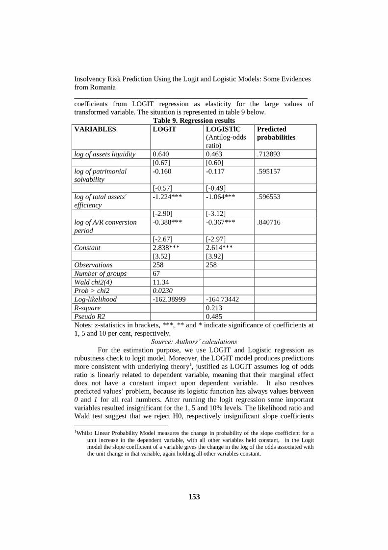
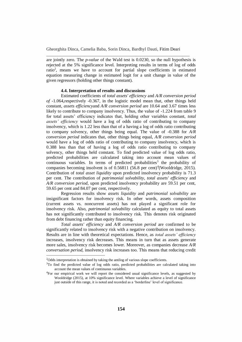
coefficients from LOGIT regression as elasticity for the large values of transformed variable. The situation is represented in table 9 below.

Table 9. Regression results

VARIABLES LOGIT LOGISTlC (Antilog-odds

ratio)

Predicted

probabilities

log of assets liquidity 0.640 0.463 .713893

[0.67] [0.60]

log of patrimonial solvability

-0.160 -0.117 .595157

[-0.57] [-0.49]

log of total assets'

efficiency

-1.224*** -1.064*** .596553

[-2.90] [-3.12]

log of A/R conversion

period

-0.388*** -0.367*** .840716

[-2.67] [-2.97]

Constant 2.838*** 2.614***

[3.52] [3.92]

Observations 258 258

Number of groups 67

Wald chi2(4) 11.34

Prob > chi2 0.0230

Log-likelihood -162.38999 -164.73442

R-square 0.213

Pseudo R2 0.485

Notes: z-statistics in brackets, ***, ** and * indicate significance of coefficients at

1, 5 and 10 per cent, respectively.

Source: Authors’ calculations

For the estimation purpose, we use LOGIT and Logistic regression as robustness check to logit model. Moreover, the LOGIT model produces predictions

more consistent with underlying theory1, justified as LOGIT assumes log of odds

ratio is linearly related to dependent variable, meaning that their marginal effect does not have a constant impact upon dependent variable. It also resolves

predicted values’ problem, because its logistic function has always values between

0 and 1 for all real numbers. After running the logit regression some important

variables resulted insignificant for the 1, 5 and 10% levels. The likelihood ratio and Wald test suggest that we reject H0, respectively insignificant slope coefficients

1Whilst Linear Probability Model measures the change in probability of the slope coefficient for a

unit increase in the dependent variable, with all other variables held constant, in the Logit model the slope coefficient of a variable gives the change in the log of the odds associated with the unit change in that variable, again holding all other variables constant.


________________________________________________________________

154

are jointly zero. The p-value of the Wald test is 0.0230, so the null hypothesis is

rejected at the 5% significance level. Interpreting results in terms of log of odds ratio2, means we have to account for partial slope coefficients in estimated

equation measuring change in estimated logit for a unit change in value of the

given regressors (holding other things constant).

4.4. Interpretation of results and discussions

Estimated coefficients of total assets' efficiency and A/R conversion period

of -1.064,respectively -0.367, in the logistic model mean that, other things held constant, assets efficiencyand A/R conversion period are 10.64 and 3.67 times less

likely to contribute to company insolvency. Thus, the value of -1.224 from table 9

for total assets’ efficiency indicates that, holding other variables constant, total assets’ efficiency would have a log of odds ratio of contributing to company

insolvency, which is 1.22 less than that of a having a log of odds ratio contributing

to company solvency, other things being equal. The value of -0.388 for A/R

conversion period indicates that, other things being equal, A/R conversion period would have a log of odds ratio of contributing to company insolvency, which is

0.388 less than that of having a log of odds ratio contributing to company

solvency, other things held constant. To find predicted value of log odds ratio, predicted probabilities are calculated taking into account mean values of

continuous variables. In terms of predicted probabilities3 the probability of

companies becoming insolvent is of 0.56811 (56.8 per cent)4(Wooldridge, 2015).

Contribution of total asset liquidity upon predicted insolvency probability is 71.3 per cent. The contribution of patrimonial solvability, total assets' efficiency and

A/R conversion period, upon predicted insolvency probability are 59.51 per cent,

59.65 per cent and 84.07 per cent, respectively. Regression results show assets liquidity and patrimonial solvability are

insignificant factors for insolvency risk. In other words, assets composition

(current assets vs. noncurrent assets) has not played a significant role for insolvency risk. Also, patrimonial solvability calculated as equity to total assets

has not significantly contributed to insolvency risk. This denotes risk originated

from debt financing rather than equity financing.

Total assets' efficiency and A/R conversion period are confirmed to be significantly related to insolvency risk with a negative contribution on insolvency.

Results are in line with theoretical expectations. Hence, as total assets’ efficiency

increases, insolvency risk decreases. This means in turn that as assets generate more sales, insolvency risk becomes lower. Moreover, as companies decrease A/R

conversation period, insolvency risk increases too. This means that reducing credit 2Odds interpretation is obtained by taking the antilog of various slope coefficients. 3To find the predicted value of log odds ratio, predicted probabilities are calculated taking into

account the mean values of continuous variables. 4For our empirical work we will report the considered usual significance levels, as suggested by

Wooldridge (2015), at 10% significance level. Where variables achieve a level of significance just outside of this range, it is noted and recorded as a ‘borderline’ level of significance.


from Romania

_________________________________________________________________

155

period to customers generated higher risk. Usually, as A/R collection period increases, future becomes more unpredictable and insolvency risk increases as

well. However, our result in this case is slightly contradictory. The explanation of

this result may be the fact that as companies shortened A/R conversation period, clients were more likely to switch to competitors, thus sales decreased.

Conclusions

Our sample with the 70 economic entities, is heterogeneous, with companies belonging to different sectors; they have different size and originate

from different geographical areas. It is well known that score functions are

appropriate for the period or economic situation in which they were created. Compared to this function, our model, comprising a set of five measures, can

provide generally valid and reliable results and allows for data generalization and

results’ implementation under any economic circumstances. Correlated analysis of economic and financial measures was meant to

shape a clearer picture regarding imminent insolvency risk for the 70 economic

entities studied. All five measure composing the model recorded a downward trend

(in the last three years preceding the entry in a state of insolvency) and values outside ranges deemed as normal for healthy companies (recording levels lower

than the minimum accepted values). From third year-on, more than 50% of

analyzed companies experienced deterioration of marked indicators. Thus 75%, respectively 85% of analyzed companies showed a negative general, respectively

patrimonial solvency, with a high level of debts toward creditors and failure to

serve their due payments. Simultaneously, for three consecutive years, there can be noticed a significant and constant increase of A/R conversion period.

Increasing delay in cashing receivables, caused mainly by commercial

credit policy relaxation and insufficient analysis of potential credit beneficiaries,

was the main insolvency reason. The increasing delays in collecting receivables led to delays in paying debt toward creditors and calling additional debt to continue

their business.

A second reason which caused many Romanian companies enter insolvency in 2013, was decrease of assets’ efficiency, as companies registered a

diminishing turnover along a lesser assets’ decrease. This latter evolution is most

likely a direct consequence of the delay of transforming receivables into cash (of

increased balance of accounts receivable). The inability to honor creditors’ obligations (general solvency with low

and declining values), accelerated de-capitalization (unsatisfactory and declining

level of economic solvency), growing delays in collecting the value of goods and services sold (increasing A/R conversion period), the lack of real liquidity

(declining assets’ liquidity) and inefficient use of assets (downward trend of assets’

efficiency) are the five measures that, together, led to a situation of imminent insolvency, within a three years’ period.


________________________________________________________________

156

Consequently, there can be seen a correlation of the five economic and

financial measures and they have fairly equal influence in their ability to forecast whether an economic entity is at risk to become insolvent and then declared

bankrupt.

However, the model has its limits and the authors do not claim that it can

substitute other tools of financial analysis, requiring supplementary statistical or econometric instruments or procedures. Meanwhile, due to the fact that the data

selection includes extremely accessible sets of information for the general public

and, implicitly, for the business environment, it represents a readily available instrument, providing an accurate prediction tool with high applicability in real life

situations.

REFERENCES

[1] Altman, E. I. (1968), Financial Ratios. Discriminant Analysis and the

Prediction of Corporate Bankruptcy; The Journal of Finance, 23(4), 589-609;

[2] Altman, E.I., Haldeman, R.G. and Narayanan, P. (1977), ZETATM Analysis;

A New Model to Identify Bankruptcy Risk of Corporations; Journal of Banking & Finance, 1(1), 29–54;

[3]Anghel, I. (2000), Bankruptcy Prediction in Romanian Enterprises ;

Economic Tribune Journal, Bucharest;

[4] Armeanu, Ș., Vintilă, G., Moscalu, M., Filipescu, M. and Lazăr, P. (2012),

Using Quantitative Data Analysis Techniques for Bankruptcy Risk Estimation

for Corporations; Theoretical and Applied Economy, 1 (566), 86-102;

[5] Beaver, W.H. (1966), Financial Ratios as Predictors of Failure; Empirical Research in Accounting. Selected Studies. Supplement to Journal of Accounting

Research, 71-111;

[6] Brigham, E. F. and Ehrhardt, M. C. (2007), Financial Management:

Theory and Practice; South-Western Cengage Learning. 14thedition;

[7] Burksaitiene D. and A. Mazintiene (2011), The Role of Bankruptcy

Forecasting in the Company Management; Economics and Management, 16,

137-143; [8] Gharaibeh, M. A., Sartawi I. S. M. and Daradkah, D. (2013), The

Applicability of Corporate Failure Models to Emerging Economies: Evidence

from Jordan; Interdisciplinary Journal of Contemporary Research in Business, 5(4), 313-325;

[9] Guerin, S. S. (2006), The Role of Geography in Financial and Economic

Integration: A Comparative Analysis of Foreign Direct Investment, Trade and Portfolio Investment Flows; The World Economy, Vol. 29, No. 2, 189–209;

[10] Hayes Suzanne K., Hodge Kay A. and Hughes, L. W. (2010), A Study of

the Efficacy of Altman’s Z to Predict Bankruptcy of Specialty Retail Firms

Doing Business in Contemporary Times; Economics & Business Journal: Inquiries & Perspectives, 3 (1), 122-134;

http://www.sciencedirect.com/science/article/pii/0378426677900176

http://www.sciencedirect.com/science/journal/03784266

http://www.sciencedirect.com/science/journal/03784266

http://www.sciencedirect.com/science/journal/03784266/1/1


from Romania

_________________________________________________________________

157

[11] Karas, M. and Režňáková, M. (2014), A Parametric or Nonparametric

Approach for Creating a New Bankruptcy Prediction Model: The Evidence from

the Czech Republic; International Journal of Mathematical Models and Methods

in Applied Sciences, 8, 214-223; [12] Kiyak, D. and Labanauskaitė, D. (2012), Assessment of the Practical

Application of Corporate Bankruptcy Prediction Models; Economics and

Management, 17 (3), 195-205;

[13] Korol T. and Korodi, A. (2011), An Evaluation of Effectiveness of Fuzzy

Logic Model in Predicting the Business Bankruptcy; Romanian Journal of

Economic Forecasting, 3, 92-107;

[14] Måns, S. (2009), Applied Econometrics-Binary Choice Models. University of Gothenburg;

[15] Ohlson, J. A. (1980), Financial Ratios and the Probabilistic Prediction of

Bankruptcy; Journal of Accounting Research, 18, 109-131; [16] Platt H. D. and Platt, M. B. (1990), Development of a Class of Stable

Predictive Variables: The Case of Bankruptcy Prediction; Journal of Business

Finance & Accounting, 17 (1), 31–51;

[17] Pereira, L. C. and Machado-Santos, C. (2007), Insolvency Prediction in

the Portuguese Textile Industry; European Journal of Finance and Banking

Research, 1(1), 16-27;

[18] Shumway, T. (2001), Forecasting Bankruptcy more Accurately: A Simple

Hazard Model; Journal of Business, 74 (1), 101-124;

[19] Szeverin, É. K. and László K. (2014), The Efficiency of Bankruptcy

Forecast Models in the Hungarian SME Sector; Journal of Competitiveness, 6 (2), 56-73;

[20] Vintilă G. and Toroapă, M.G. (2012a), Bankruptcy Prediction Model for

Listed Companies in Romania; Journal of Eastern Europe Research in Business

& Economics, Article ID 381337, DOI: 10.5171/2012.3811337; [21] Wooldridge, Jeffrey M. (2015), Introductory Econometrics: A Modern

Approach. Nelson Education;

[22] Zheng Q. and Yanhui, J. (2007), Financial Distress Prediction on Decision

Tree Models; Paper presented at Service Operations and Logistics, and

Informatics (SOLI) IEEE, Philadelphia, USA;

[23] Zeytınoglu. E. and Akarım, Y. D (2013), Financial Failure Prediction

Using Financial Ratios: An Empirical Application on Istanbul Stock Exchange; Journal of Applied Finance & Banking 3(3), 107-116;

[24] Zmijewski, M. (1984), Methodological Issues Related to the Estimation of

Financial Distress Prediction Models; Journal of Accounting Research, 22 (Supplement), 59-82.

http://onlinelibrary.wiley.com/doi/10.1111/jbfa.1990.17.issue-1/issuetoc

Documents

Associate Professor Mirela Camelia BABA, PhD - Dinca Gheorghita, Dinca...Gheorghita Dinca, Camelia Baba, Sorin Dinca, Bardhyl Dauti, Fitim Deari _____ 140 by their companies), as well