Embed Size (px)
Citation preview
Asteroseismology of
16 Cyg A and B
João Pedro de Sousa Faria Mestrado em Astronomia Departamento de Física e Astronomia
2013
Orientador Mário João Pires Fernandes Garcia Monteiro,
Professor Associado, Faculdade de Ciências da Universidade do Porto
Coorientador Margarida Maria Salvador Cunha,
Investigadora Principal, Centro de Astrofísica da Universidade do Porto


Acknowledgments
This work would not have been possible without the help and guidance of my super-visors, Dr. Mário João Monteiro and Dr. Margarida Cunha. I would like to express mysincere gratitude to both. Besides being outstanding researchers, they have proven to beremarkable teachers and their expertise, insight, and patience added considerably to myexperience. I was lucky to learn how to do science from two of the best scientists I know.The following, more personal, acknowledgments have no need to be in English.Sem a ajuda generosa e altruísta da minha amiga Brígida, a aventura que foram estes
dois anos numa cidade nova, com pessoas novas, com experiências novas, não teria sidosequer imaginável. Um sincero obrigado, pelo apoio e pela amizade.Por último, gostaria de agradecer à minha mãe, por tudo, desde o primeiro dia (na
verdade, desde o primeiro dia menos nove meses). Fizeste tudo bem, à primeira tentativa.
i

Abstract
The Kepler space telescope has produced very precise long-term photometric time seriesdata for thousands of stars in its quest to find planets similar to Earth. The data allowedthe detection of solar-like oscillations in a wide range of stellar types, from giants tosubdwarfs. Stellar oscillations allow us to improve structure and evolution models becausethey are the only observables probing the internal properties of stars.The correct use of all the information contained in the oscillation frequencies can
provide very precise estimates of the masses, radii, ages and chemical abundances of stars.The study of the available diagnostics tools that use only data that can be observed instars other than the Sun is thus valuable in order to explore the full potential of currentand future observations.In this work, I focus on two particular sources, the components of the 16 Cyg binary,
and use asteroseismic tools to extract information about their interior regions. I performmodel fitting of the observed frequencies and investigate the so called acoustic glitches– regions with an abrupt change in the stratification of the star – and their effect on theobserved oscillation frequencies.
Keywords. asteroseismology – stars: solar-type – stars: evolution – stars: interiors – stars:oscillations – methods: data analysis
iii

Resumo
O telescópio espacial Kepler, na sua demanda por planetas similares à Terra, obteve sériestemporais de fotometria para milhares de estrelas, com uma precisão e duração inéditas.Estes dados permitiram a deteção de oscilações do tipo solar em estrelas com uma vastagama de tipos espectrais. O estudo destas oscilações, que são os únicos observáveisque transportam informação detalhada sobre o interior das estrelas, permite melhorar osmodelos de estrutura e evolução estelar.A correcta utilização de toda a informação contida nas frequências de oscilação pode
levar a determinações bastante precisas da massa, raio, idade e abundâncias químicas dasestrelas. O estudo das ferramentas de diagnóstico dos interiores estelares que precisamapenas do mesmo tipo de dados que são observáveis noutras estrelas é, então, uma maisvalia na exploração de todo o potencial das observações presentes e futuras.
Neste trabalho, focado nos componentes do binário 16 Cyg em particular, estudo al-gumas aplicações dos dados de asterosismologia para extrair informação sobre as regiõesinteriores destas estrelas. Modelos de evolução estelar são ajustados às frequências ob-servadas e os chamados acoustic glitches – regiões onde a estratificação da estrela mudabruscamente – bem como as formas de os detectar são também estudados.
Palavras-chave. asterosismologia – estrelas: tipo solar – estrelas: evolução – estrelas:interiores – estrelas: oscilações – métodos: análise de dados
v

Contents
1 introduction 12 stellar oscillations and diagnostic tools 5
2.1 Basic Oscillation Equations 52.2 Asymptotic analysis 72.3 Frequency combinations 11
3 measuring acoustic glitches 173.1 Nature of the signal 173.2 Complete expressions 203.3 Methods to isolate the signals 233.4 Code validation - signal in solar frequencies 273.5 Amplitude magnification 29
4 the solar-type stars 16 cyg a & b 334.1 Stellar properties 334.2 Kepler observations 344.3 Model fitting 374.4 Acoustic glitches 444.5 Calibrating the surface Helium abundance 51
5 conclusion 53
bibliography 56
vii
List of Figures
Fig. 1.1 Power spectra of solar-like oscillations for representative stars. 2Fig. 2.1 Trapping regions of p and g modes. 9Fig. 2.2 Amplitude spectra of solar oscillations measured by the VIRGO
instrument on SOHO. 11Fig. 2.3 Échelle diagrams for frequencies of the Sun. 12Fig. 2.4 Small separations d02 and ratios r02 for four models of the Sun. 13Fig. 3.1 Acoustic potentials. 18Fig. 3.2 Adiabatic exponent Γ1 for different solar models. 21Fig. 3.3 Fits to the solar frequencies using the improved Method 1. 28Fig. 3.4 Fits to the solar second differences using Method 2. 29Fig. 3.5 Amplitude magnification for 16 Cyg A and B. 31Fig. 4.1 Position of the Sun and 16 Cyg A and B on the Hertzsprung-Russel
diagram. 34Fig. 4.2 Observational échelle diagrams of 16 Cyg A and B. 37Fig. 4.3 Evolutionary tracks of the best models for 16 Cyg A. 40Fig. 4.4 Échelle diagrams with the best model frequencies. 42Fig. 4.5 Large frequency separations for best model of 16 Cyg A. 43Fig. 4.7 Frequency ratios from the best models and from observations. 44Fig. 4.8 Signal fit obtained with Method 1 in the frequencies of 16 Cyg A
and B. 45Fig. 4.9 Histograms of the fitted values of ABCZ and AHeIIZ for Monte Carlo
realizations of the frequencies (Method 1). 45Fig. 4.10 Histograms of the fitted values of τHeIIZ and τBCZ for Monte Carlo
realizations of the frequencies (Method 1). 45Fig. 4.11 Signal fit obtained with Method 2 in the second differences of 16
Cyg A and B 46Fig. 4.12 Histograms of the fitted values of ABCZ and AHeIIZ for Monte Carlo
realizations of the frequencies (Method 2). 47Fig. 4.13 Histograms of the fitted values of τHeIIZ and τBCZ for Monte Carlo
realizations of the frequencies (Method 2). 47Fig. 4.14 Amplitudes and acoustic locations obtained with both methods for
16 Cyg A and B. 50
viii
Fig. 4.15 Temperature gradients for the best models of 16 Cyg A and B. 50Fig. 4.16 Calibration of Helium surface abundance for 16 Cyg A and B. 52
In all figures where it applies and is not stated otherwise, we use the following symboland color convention:
` = 0 points represented by red stars
` = 1 points represented by green circles
` = 2 points represented by blue diamonds
` = 3 points represented by magenta squares.
List of Tables
Table 4.1 Properties of 16 Cyg A & B. 34Table 4.3 Observed oscillation frequencies for 16 Cyg A and B from nine
months of Kepler data. 36Table 4.4 Model fitting results for 16 Cyg A & B. 42Table 4.5 Properties of the parameter distributions from Monte Carlo simu-
lations of the fit to the frequencies. 46Table 4.6 Properties of the parameter distributions from Monte Carlo simu-
lations of the fit to the second differences. 48Table 4.7 Signal parameters and associated uncertainties for the best MESA
models (with overshoot), obtained from Methods 1 and 2. 49
Listings
The MESA inlist files and open-source versions of both detection methods are avail-able online at https://www.astro.up.pt/~jfaria/msc-thesis.
ix

1Introduction
It is becoming standard practice to cite Eddington in general introductions related toasteroseismology. A standard from which I will not deviate:
Ordinary stars must be viewed respectfully like objects in glass cases inmuseums; our fingers are itching to pinch them and test their resilience.Pulsating stars are like those fascinating models in the Science Museumprovided with a button which can be pressed to set the machinery in motion.To be able to see the machinery of a star throbbing with activity is mostinstructive for the development of our knowledge.
– A.S. Eddington, Stars and Atoms, Oxford University Press, 1927
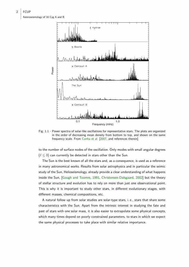
Asteroseismology is the science that studies the internal structure of pulsating starsby interpreting their frequency spectra. The size, temperature and brightness of thesestars vary periodically by a very small but measurable amount (a fraction of a degree intemperature and a few parts per million in brightness, for a star like the Sun). Thesevariations will also cause radial velocity and line profile changes. Therefore, pulsating starscan be studied photometrically and spectroscopically, with time series measurements. Byperforming a frequency analysis of the time series it is possible to identify oscillationpatterns, often with a large number of dominant frequencies (see Figure 1.1).Different frequencies correspond to different oscillation modes that provide information
about the interior regions of the star because they are the surface manifestations of soundwaves trapped inside the star.
In a manner that is very similar to how a seismologist uses earthquakes to probe theinterior of the Earth, an asteroseismologist probes the interior of stars by studying theirnatural oscillation modes.One difference to geoseismology is that the surfaces of stars other than the Sun
are not resolved by current observations, which means that inference about the stellarinteriors needs to rely on oscillation modes that do not cancel out when disk-integratedmeasurements are made. The modes of spherically symmetric stars are characterized byeigenfunctions that are proportional to the spherical harmonics Y`m with the quantumnumbers obeying ` = 0, 1, 2, . . . ;m = 0,±1, . . . ,±`. The angular degree ` corresponds
1
2 FCUPAsteroseismology of 16 Cyg A and B
Fig. 1.1 - Power spectra of solar-like oscillations for representative stars. The plots are organizedin the order of decreasing mean density from bottom to top, and shown on the samefrequency scale. From Cunha et al. [2007, and references therein]
to the number of surface nodes of the oscillation. Only modes with small angular degrees(` ≤ 3) can currently be detected in stars other than the Sun.
The Sun is the best known of all the stars and, as a consequence, is used as a referencein many astronomical works. Results from solar astrophysics and in particular the seimicstudy of the Sun, Helioseismology, already provide a clear understanding of what happensinside the Sun, [Gough and Toomre, 1991, Christensen-Dalsgaard, 2002] but the theoryof stellar structure and evolution has to rely on more than just one observational point.This is why it is important to study other stars, in different evolutionary stages, withdifferent masses, chemical compositions, etc.A natural follow up from solar studies are solar-type stars, i. e., stars that share some
characteristics with the Sun. Apart from the intrinsic interest in studying the fate andpast of stars with one solar mass, it is also easier to extrapolate some physical concepts,which many times depend on poorly constrained parameters, to stars in which we expectthe same physical processes to take place with similar relative importance.
FCUP 3
Asteroseismology of 16 Cyg A and B
The precise data available from space missions like Kepler † [Gilliland et al., 2010]has made possible asteroseimic investigations that cover a broad range of stellar prop-erties and evolutionary stages. In particular, the clear detection of dozens of oscillationfrequencies on distant solar-like stars [e. g. Chaplin et al., 2011] has provided a meansto study their interiors, which seemed inaccessible before. However, it has also exposedsome issues with current state of the art stellar models.The modelling of the near-surface regions of a solar-like star is still deficient as it ignores
dynamical effects of convection. Also, frequency calculations are almost always carriedout in the adiabatic approximation, even though the oscillations are definitely not in thisregime in the superficial layers [e. g. Houdek, 2010]. These and other uncertainties instellar modelling mean that the naive comparison between observed values of frequenciesand those computed from models will not be an optimal procedure, despite its simplicity.This is because it is affected by a global average of all the uncertainties, even if someare not pertinent to a particular calibration.There are three different ways to circumvent these difficulties: a) apply a correction to
the model frequencies that can eliminate the systematic differences to the observations[Kjeldsen et al., 2008] and carry on with the search for the best fitting model parameters;b) Consider combinations of frequencies constructed in such a way that they will beinsensitive to certain aspects of the stellar modeling, and compare those with observedvalues calculated in the same manner; c) rely on properties of the frequencies (or of thefrequency combinations) that depend only on a very specific region of the star, for whichan example may be the oscillatory signals produced in the frequencies by regions of rapidvariation of the stellar structure, the so called acoustic glitches [Gough, 1990].
In this work I study the last two options and use them to extract detailed informationabout the interiors of two particular stars, the components of the binary system 16 Cygni.Binaries are important science cases because one can usually decrease the degrees offreedom of the problem, assuming identical initial chemical compositions and ages forboth stars of the system. Being very bright targets, the quantity and quality of availabledata for the two stars are also exquisite.Several frequency combinations, that extend beyond the more common large and small
separations will be discussed and used to improve the forward modelling approach. Theyare applied to the 16 Cygni data and an inference is made on the best model parametersfor each star, building on results of previous works [Metcalfe et al., 2012]. The bestmodels are expected to reproduce well the interior regions of the stars.
†There has been no space telescope completely dedicated to asteroseismology, though the French-ledCoRoT mission stated it as one of its core objectives [e. g. Baglin et al., 2007]. Kepler was launchedin 2009, and although originally designed to search for earth-like planets, it has been very effective inperforming asteroseismic measurements, providing extremely precise and long time series photometry forhundreds of stars.
4 FCUPAsteroseismology of 16 Cyg A and B
To obtain the stellar models I will be using a fairly recent stellar evolution code, MESA(Modules for Experiments in Stellar Astrophysics, [Paxton et al., 2011, 2013]). The codeis completely open-source and has already built a community of users, which providesa fair amount of technical support and encourages sharing and reproducibility of results.Despite being open-source MESA is not, by all means, simple. It is a fully modularcode that uses comprehensive and up-to-date microphysics and solves the structure andevolution equations with modern techniques, targeted at modern computers. MESAstar is the name of the stellar evolution code itself that makes use of all the physicsand mathematics modules to build and evolve stellar models. For the calculation ofoscillation frequencies for the models, MESA has been integrated with ADIPLS, theAarhus adiabatic oscillation package [Christensen-Dalsgaard, 2008].
A second part of this work is focused on the oscillatory signals present in the oscil-lation frequencies that are caused by the rapid structural variations at the base of theconvection zone and at the Helium second ionization region (from now on, BCZ andHeIIZ, respectively). By detecting and characterizing these signals one can expect toconstrain not only the position of the corresponding regions inside the star but alsoother stellar parameters related to the physical cause of the signals, such as the surfaceHelium abundance. For the Sun, this has been extensively studied before [Monteiro andThompson, 2005, and references therein] and for other stars the best methods are stillbeing developed [Mazumdar et al., 2012]The end goals of this thesis are the construction of models that reproduce the observed
characteristics of the two stars, the detailed description of the acoustic glitches and theireffect on the oscillation frequencies, as well as the description of the methods usedto detect them and how they can be used to calibrate the surface Helium abundanceof 16 Cyg A & B. The dissertation is organized as follows: in the following chapter(Chapter 2) the theoretical basis of asteroseismology of solar-type stars is briefly reviewedand the frequency combinations that can be used as diagnostics of the stellar interiorsare presented and justified. Chapter 3 introduces acoustic glitches, the reasons for thepresence of an oscillatory signal in the frequencies and the methods used to detect thissignal. Our own implementations and improvements to these methods are described indetail and validated using solar data. In Chapter 4 the main focus is drawn to 16 CygA & B, the available Kepler data is listed together with the results obtained for themodelling and the acoustic glitch characterization. Preliminary results on an attempt tocalibrate the Helium surface abundance are presented next and in Chapter 5, I discussthe main results and draw some final conclusions.
2Stellar Oscillations and Diagnostic Tools
From a theoretical perspective, we start by understanding where the diagnostic potentialof stellar oscillations comes from. With only a few assumptions about the equilibriumbackground state of the star, which is perturbed to obtain a basic description of theoscillations, we can already grasp some of the dependence of the oscillation frequencieson the stellar interior. This theoretical description will allow for an interpretation of theobserved frequencies.In this chapter a brief introduction to the theory of stellar oscillations is presented,
together with some results from the asymptotic theory. The expressions for differentfrequency combinations are also shown and will serve as diagnostic tools to probe specificregions of the stellar interior.
2.1 Basic Oscillation Equations
The adiabatic oscillations of a spherically symmetric star are described by the standardequations of fluid mechanics
ρdu
dt+∇P + ρ∇Φ = 0 (equation of motion)
dρ
dt+ ρ∇ · u = 0 (mass conservation)
1
p
dP
dt− Γ1
ρ
dρ
dt= 0 (adiabatic condition)
∇2Φ = 4πGρ (Poisson's equation)
(2.1)
where u, P , ρ, Φ, Γ1 are the velocity, pressure, density, gravitational potential andfirst adiabatic exponent, respectively. The derivative following the motion of the gas,d/dt = ∂/∂t+ u ·∇, is the Lagrangian (or material) time derivative. This Lagrangian formof the equations is often used since it simplifies some of the equations. The adiabaticcondition results from the energy equation when we consider that no heat is exchangedduring the oscillations.
5
6 FCUPAsteroseismology of 16 Cyg A and B
If there are no velocities and the system is static, so that u = 0 and all time derivativescan be neglected, we say the system is in equilibrium and equations (2.1) reduce to theequations of the hydrostatic structure of a spherical star
dp0dr
= −gρ0 , g =dΦ0
dr=GMr
r2,
dMr
dr= 4πGρ0r
2
withMr the mass inside a sphere with radius r and G the gravitational constant. Here,we use the subscript 0 (zero) to refer to the equilibrium structure.
Considering small amplitude perturbations around the equilibrium state we write
u =d(δr)dt
, p = p0 + p′, ρ = ρ0 + ρ′, Φ = Φ0 + Φ′
where quantities with a superscript are small, time dependent, Eulerian perturbations.Note that the perturbations are not necessarily spherically symmetric. We seek solutionsfor the perturbations with time dependence given by eiωt, with a frequency ω. Given theassumption that the equilibrium state is spherically symmetric, the dependence of theperturbations on the angular variables (θ, φ) can be separated from that on the radialvariable r by means of spherical harmonics Y`m. Here, ` and m are integers such that` ≥ 0 and |m| ≤ `. We then write the perturbations as
δr =
(ξ(r), ζ(r)
∂
∂θ, ζ(r)
∂
sin θ∂φ
)Y`me
iωt
p′ = p(r)Y`meiωt
Φ′ = Φ(r)Y`meiωt
(2.2)
allowing us to write the equations of small amplitude adiabatic oscillations
dξ
dr+
(2
r− g
c2
)ξ +
(1− S2
l
w2
)p′
ρc2− `(`+ 1)
w2r2Φ′ = 0
dp′
dr+g
c2p′ +
(N2 − w2
)ρξ + ρ
dΦ′
dr= 0
d2Φ′
dr2+
2
r
dΦ′
dr− `(`+ 1)
r2Φ′ − 4πGρ
(p′
ρc2+N2
gξ
)= 0
(2.3)
In Eqs. (2.3), we introduced the adiabatic sound speed c given by
c2 = Γ1p
ρ
and two characteristic frequencies: the Lamb (or acoustic) frequency S`
S2` =
`(`+ 1)c2
r2
and the Brunt-Väisälä (or buoyancy) frequency N
FCUP 7
Asteroseismology of 16 Cyg A and B
N2 = −g2
c2
(1− Γ1
d log ρ
d log p
)
Note that all the terms in Eqs. (2.3) are independent of m as a consequence of thespherical symmetry of the equilibrium state. This degeneracy is lifted by rotation.This system of homogeneous equations is of fourth order and must satisfy four bound-
ary conditions at the center (r = 0) and at the surface (r = R) of the star [Unno et al.,1989, chapter 14].
The equations and boundary conditions have non-trivial solutions only for specificvalues of the frequency ω, which is therefore an eigenvalue of the problem. We call eachsolution, corresponding to both the eigenfrequency ωn` and the eigenfunction (the run ofthe perturbations ξ, p′, etc. with r) a mode of oscillation. The radial order n correspondsessentially to the number of zeros in the radial direction in the eigenfunctions.Due to their homogeneity, Eqs. (2.3) only determine the solution up to a constant
factor; the amplitude of the perturbations is not determined in the linear approximation.
2.2 Asymptotic analysis
Analytical solutions to the full set of equations of adiabatic oscillations exist only invery particular cases (like the case of an isothermal atmosphere or a non-gravitatingsphere [Aerts et al., 2010]). The full fourth order system can be solved numerically,but some insight might be obtained by making a simplifying assumption, the so calledCowling approximation. This will allow us to write a general but approximate second-order differential equation for ξ, define the propagation region of p modes and simplifythe subsequent asymptotic analysis needed to construct diagnostic tools.
Cowling approximation
Together with the system of three equations mentioned above, the perturbation to thegravitational potential Φ′ also satisfies the perturbed Poisson equation
∇2Φ′ = 4πGρ′ (2.4)
or in separated form
1
r2
d
dr
(r2dΦ′
dr
)− `(`+ 1)
r2Φ′ = 4πGρ′ (2.5)
which has the integral solution (can be verified by substitution in 2.5)
8 FCUPAsteroseismology of 16 Cyg A and B
Φ′(r) = − 4πG
2`+ 1
[1
r`+1
∫ r
0ρ′ (r′)`+2dr′ + r`
∫ R
r
ρ′
(r′)`−1dr′]
(2.6)
From Eq. (2.6) it follows that Φ′ is small compared to ρ′ in one of two cases: if `is large or if the radial order |n| is large [Cowling, 1941]. Under one or both of thesecircumstances, it is reasonable, and indeed accurate, to neglect the perturbation to thegravitational potential, Φ′ [Christensen-Dalsgaard, 1991]. By doing that, the oscillationequations can be written in the form
dξ
dr= −
(2
r− g
c2
)ξ −
(1− S2
l
w2
)p′
ρc2
dp′
dr=
g
c2p′ +
(w2 −N2
)ρξ
(2.7)
The two equations in Eq. (2.7) can be combined in a single second-order differentialequation if we neglect the derivatives of g and r (basically, this means assuming thatthe oscillations vary more rapidly than g and r so that, locally, the problem is one ofoscillations in a plane-parallel layer under constant gravity). The result is the equation[e. g. Deubner and Gough, 1984]
d2X
dr2+
1
c2
[S2`
(N2
ω2− 1
)+ ω2 − ω2
c
]X = 0 (2.8)
for the quantity X = c2ρ1/2divδr. Here we have introduced the acoustic cut-offfrequency
ω2c =
c2
4H2
(1− 2
dH
dr
)
where H = −(d ln ρ/dr)−1 is the density scale height. The main properties of theeigenfunctions that are solution of (2.8) are determined by the properties of
K ≡ 1
c2
[S2`
(N2
ω2− 1
)+ ω2 − ω2
c
]
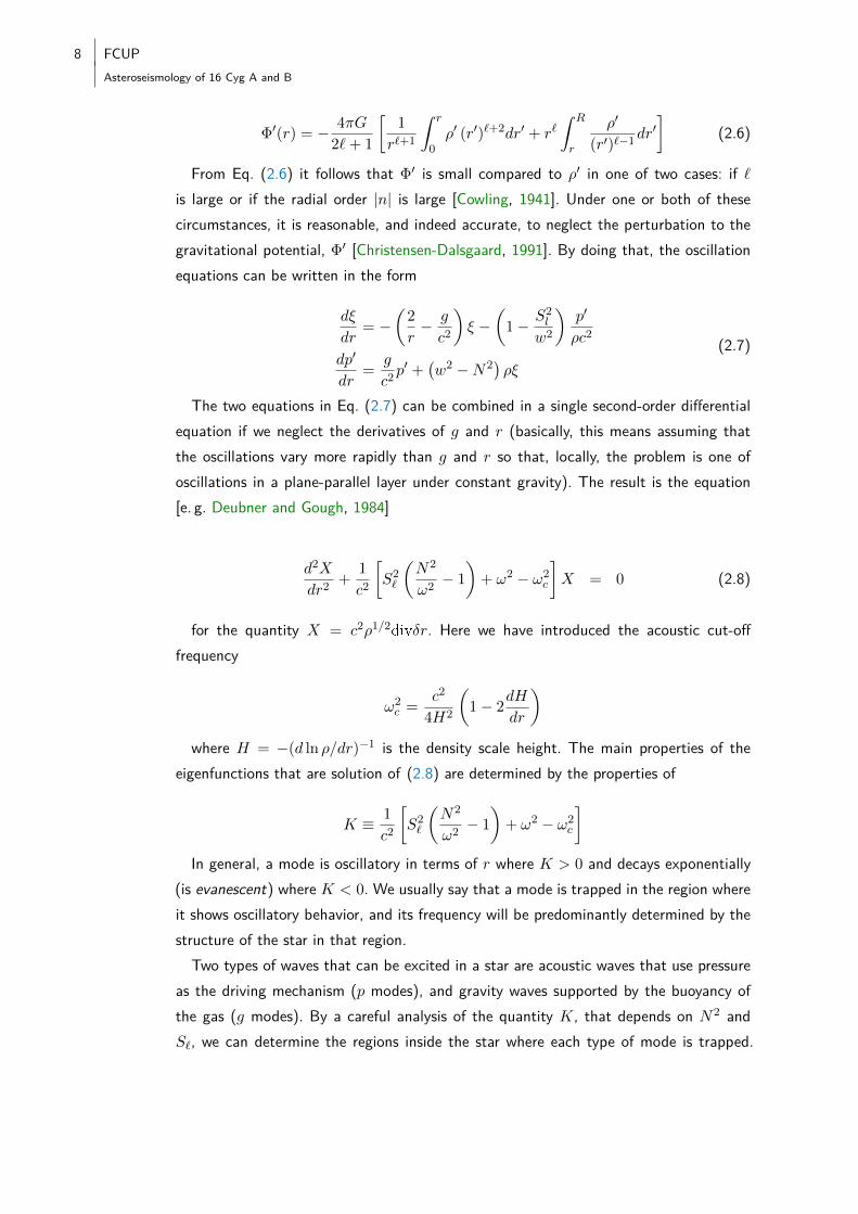
In general, a mode is oscillatory in terms of r where K > 0 and decays exponentially(is evanescent) where K < 0. We usually say that a mode is trapped in the region whereit shows oscillatory behavior, and its frequency will be predominantly determined by thestructure of the star in that region.Two types of waves that can be excited in a star are acoustic waves that use pressure
as the driving mechanism (p modes), and gravity waves supported by the buoyancy ofthe gas (g modes). By a careful analysis of the quantity K, that depends on N2 andS`, we can determine the regions inside the star where each type of mode is trapped.
FCUP 9
Asteroseismology of 16 Cyg A and B3.4 Asymptotic Theory of Stellar Oscillations 205
Fig. 3.14. Buoyancy frequency N [cf. Eq. (3.155); continuous line] and char-acteristic acoustic frequency Sl [cf. Eq. (3.153); dashed lines, labelled by thevalues of l], shown in terms of the corresponding cyclic frequencies, againstfractional radius r/R for a model of the present Sun. The heavy horizontallines indicate the trapping regions for a g mode with frequency ν = 100μHz,and for a p mode with degree 20 and ν = 2000μHz.
centre is associated with the increase towards the centre in the helium abun-dance in the region where nuclear burning has taken place. Here, effectively,lighter material is on top of heavier material, which adds to the convectivestability and hence increases N . This is most easily seen by using the idealgas law for a fully ionized gas, Eq. (3.19) which is approximately valid in theinterior of cool stars, to rewrite N2 as
N2 � g2ρ
p(∇ad − ∇ + ∇μ) , (3.180)
corresponding to the convective instability condition written in the form givenby Eq. (3.94) (see also Eq. (3.95)). In the region of nuclear burning, μ increaseswith increasing depth and hence increasing pressure, and therefore the termin ∇μ makes a positive contribution to N2.
The behaviour of N is rather more extreme in stars with convective cores;this is illustrated in Fig. 3.15 for the case of a 2.2 M� evolution sequence. Theconvective core is fully mixed and here, therefore, the composition is uniform,with ∇μ = 0. However, in stars of this and higher masses the convective coregenerally shrinks during the evolution, leaving behind a steep gradient in the
Fig. 2.1 - Brunt-Väisälä frequency N (solid line) and Lamb frequency S` (dashed lines, labeledby the values of `), shown in terms of the corresponding cyclic frequencies, againstfractional radius r/R for a model of the Sun. The horizontal lines indicate the trappingregions for a g mode with frequency ν = 100µHz, and for a p mode with degree 20and ν = 2000µHz. From Aerts et al. [2010].
Typical regions where p and g modes are trapped are shown in Figure 2.1 for a model ofthe Sun.By JWKB analysis† of the asymptotic equation (2.8), it is possible to show that
the eigenfrequencies of low-degree p modes satisfy the relation (Gough [1993], see alsoTassoul [1980, 1990])
νn` =ωn`2π'(n+
`
2+
1
4+ α
)∆ν0 − [A`(`+ 1)− δ] ∆ν2
0
νn`(2.9)
where
∆ν0 =
(2
∫ R
0
dr
c
)−1
A =1
4π2∆ν0
[c(R)
R−∫ R
0
dc
dr
dr
r
]
and α and δ are quantities related to the near-surface region.
†Basically, the JWKB method assumes a solution of Eq. (2.8) that varies rapidly compared withequilibrium quantities, i. e., compared with K(r). This solution is written in the form X(r) ∼ exp[iΨ(r)]where Ψ is rapidly varying. After substitution back into (2.8) the powers of kr = dΨ/dr are equated andan approximate solution for X(r) is obtained to the desired order. See Aerts et al. [2010, Chap. E.3] andalso Gough [2007].
10 FCUPAsteroseismology of 16 Cyg A and B
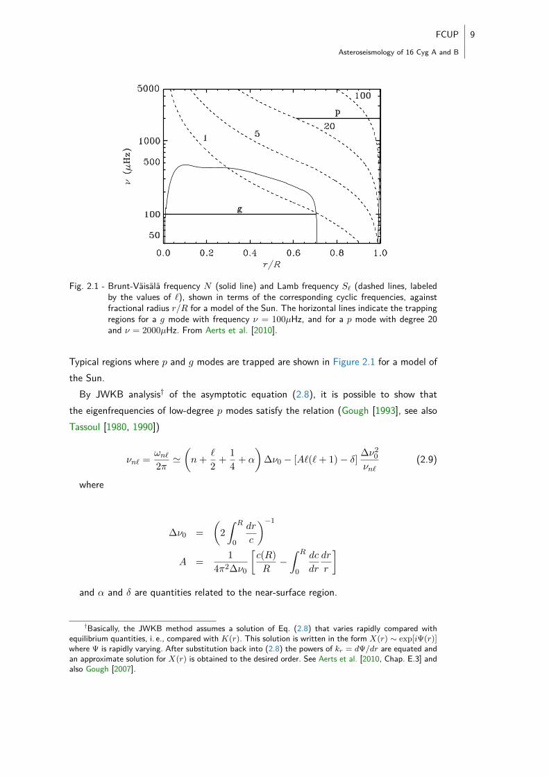
Neglecting the last second-order term, Eq. (2.9) predicts a uniform spacing betweenmodes of the same angular degree ` and consecutive radial order (see Figure 2.2). Thisdifference is known as the large frequency separation
∆νn` = νn+1 ` − νn` (2.10)
and is approximately equal to ∆ν0 in a first approximation. Moreover, we can alsopredict a degeneracy between modes with the same parity (same value of n+ `/2)
νn ` ' νn−1 `+2 (2.11)
Departure from the degeneracy in Eq. (2.11) is measured by the small frequencyseparations
d`,`+2 = νn ` − νn−1 `+2 (2.12)
which can be related to the second order term in (2.9) and shown to be
d`,`+2 ' − (4`+ 6)∆ν0
4π2νn`
∫ R
0
dc
dr
dr
r(2.13)
Another small separation that uses modes of degree ` = 0, 1 can carry equivalentinformation
d`,`+1 = νn ` −1
2(νn−1 `+1 + νn `+1) (2.14)
' − (2`+ 2)∆ν0
4π2νn `
∫ R
0
dc
dr
dr
r
The above equations show the sensitivity of the small separations to the sound speedgradient near the core of the star which is itself very sensitive to the composition profilein that region. The small frequency separations thus present an important diagnostic ofstellar evolution and stellar age.One convenient way to illustrate schematically the frequency structure that results from
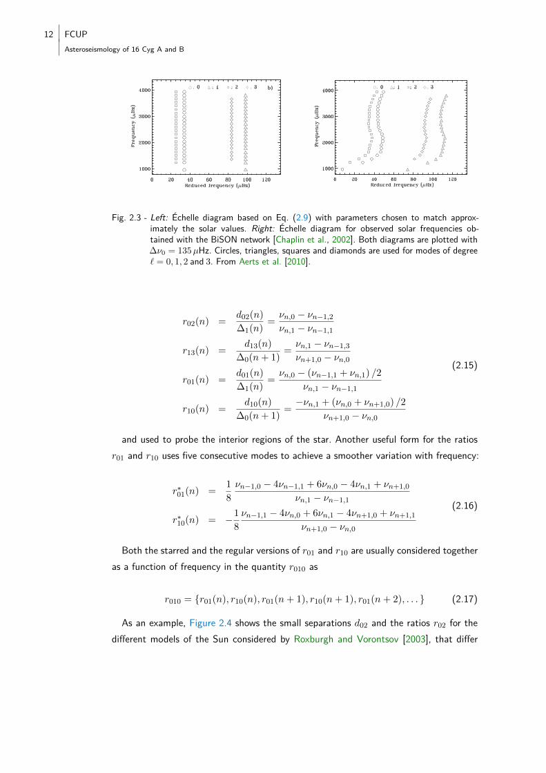
Eq. (2.9) is to use the so-called échelle diagram‡ where the frequency axis is cut intopieces of length ∆ν0 which are stacked on top of each other. This yields points arrangedin vertical lines corresponding to different values of `, each separated by the appropriatesmall separation (Figure 2.3). It is clear from the figure that the observed frequenciesshow departures from the asymptotic behaviour, although the general structure is as
‡A commonly used citation when referring to this diagram is the work of Grec et al. [1983], althoughthe word échelle (French for ladder or scale) is never mentioned in this work and its first use is indeedunknown to the author.
FCUP 11
Asteroseismology of 16 Cyg A and B
Fig. 2.2 - Amplitude spectra of solar oscillations measured by the VIRGO instrument on SOHO. Asmall portion of the solar oscillation spectrum is shown, as well as the large separations(identified only by the relevant ` subscript) and small separations d02 and d13. Eachfrequency peak is labeled with the (n, `) values of the oscillation mode. Adapted from[Catala, 2009]
expected. The curvature of the lines results from the structure near the solar surface andthe combined effects of α and δ. Also, the small separations clearly vary with frequency.
2.3 Frequency combinations
In the discussion above I have already described the large and small separations: twocombinations of the oscillation frequencies that are sensitive to different aspects of thestellar interior. It is possible to derive further relationships that will allow us to isolatespecific regions of the star and extract information about them.The predicted photometric amplitudes of the modes with degrees ` = 0, 1 are con-
siderably larger than those with ` = 2, 3 [e. g. Aerts et al., 2010]. For some stars thismay constitute a problem when calculating the small separations that need consecutivemodes. Nevertheless, and particularly for solar-type stars, there has been a substantialincrease in the number of modes detected. For the two stars that this work focuses on,a clear detection of ` = 3 modes has been made in the Kepler data, although the inher-ent uncertainties are still high (see Section 4). We are thus interested in the diagnosticpotential of frequency combinations that may involve ` = 0, 1, 2, 3 modes.
2.3.1 Signatures of the interior regions
One useful diagnostic is the ratio of small to large separations, which is essentially inde-pendent of the structure of the outer layers of the star, as was shown by Roxburgh andVorontsov [2003], Otí Floranes et al. [2005]. Different ratios can be constructed, such as
12 FCUPAsteroseismology of 16 Cyg A and B
218 3 Theory of Stellar Oscillations
Fig. 3.19. Schematic oscillation spectrum (a) and echelle diagram (b), basedon Eq. (3.223); the parameters, Δν0 = 135μHz, D0 = 1.5μHz and ε0 = 1.4,were chosen to match approximately the solar values. In panel (a) the am-plitudes were chosen as the sensitivities of Doppler-velocity observations indisc-integrated light (cf. Fig. 7.1).
From an observational point of view, and to illustrate its structure, it isconvenient to represent the spectrum by the average quantities Δν0 and D0,with
〈νn+1 l − νnl〉nl = Δν0 , δνl ≡ 〈νnl − νn−1 l+2〉n � (4l + 6)D0 (3.222)
(e.g., Scherrer et al. 1983), such that
νnl � Δν0
(n+
l
2+ ε0
)− l(l + 1)D0 , (3.223)
464 7 Applications of Asteroseismology
Fig. 7.4. Echelle diagram for observed solar frequencies obtained with theBiSON network (Chaplin et al. 2002a), plotted with ν0 = 830μHz and Δν =135μHz (cf. Eq. (3.224)). Circles, triangles, squares and diamonds are used formodes of degree l = 0, 1, 2 and 3, respectively.
half the modes illustrated the relative standard error is well below 10−5, thussubstantially exceeding the precision with which the solar mass is known.
As discussed in Section 7.1.2 the m dependence of the frequencies is oftenparameterized in terms of the so-called a coefficients (cf. Eq. (7.9)). To illus-trate this, Fig. 7.6 shows the first three odd a coefficients from MDI observa-tions. It may be shown that a1 is determined by the spherically symmetriccomponent of the angular velocity Ω(r, θ), while the higher-order coefficientsdepend on the latitude variation of Ω (see also Section 3.8.4). In particular,as discussed in Section 7.1.8, the decrease of a3 for modes with turning pointrt in the radiative interior reflects the nearly latitude-independent rotation inthis region.
As discussed in Section 7.1.2, frequencies for individual modes can be de-termined up to degrees around 200. For higher degree the modes merge intoridges of power, substantially complicating the analysis (for a review, see Re-iter et al. 2004); thus, although results on high-degree mode frequencies havebeen published (e.g., Bachmann et al. 1995) they have so far seen relatively
Fig. 2.3 - Left: Échelle diagram based on Eq. (2.9) with parameters chosen to match approx-imately the solar values. Right: Échelle diagram for observed solar frequencies ob-tained with the BiSON network [Chaplin et al., 2002]. Both diagrams are plotted with∆ν0 = 135µHz. Circles, triangles, squares and diamonds are used for modes of degree` = 0, 1, 2 and 3. From Aerts et al. [2010].
r02(n) =d02(n)
∆1(n)=νn,0 − νn−1,2
νn,1 − νn−1,1
r13(n) =d13(n)
∆0(n+ 1)=νn,1 − νn−1,3
νn+1,0 − νn,0
r01(n) =d01(n)
∆1(n)=νn,0 − (νn−1,1 + νn,1) /2
νn,1 − νn−1,1
r10(n) =d10(n)
∆0(n+ 1)=−νn,1 + (νn,0 + νn+1,0) /2
νn+1,0 − νn,0
(2.15)
and used to probe the interior regions of the star. Another useful form for the ratiosr01 and r10 uses five consecutive modes to achieve a smoother variation with frequency:
r∗01(n) =1
8
νn−1,0 − 4νn−1,1 + 6νn,0 − 4νn,1 + νn+1,0
νn,1 − νn−1,1
r∗10(n) = −1
8
νn−1,1 − 4νn,0 + 6νn,1 − 4νn+1,0 + νn+1,1
νn+1,0 − νn,0
(2.16)
Both the starred and the regular versions of r01 and r10 are usually considered togetheras a function of frequency in the quantity r010 as
r010 = {r01(n), r10(n), r01(n+ 1), r10(n+ 1), r01(n+ 2), . . . } (2.17)
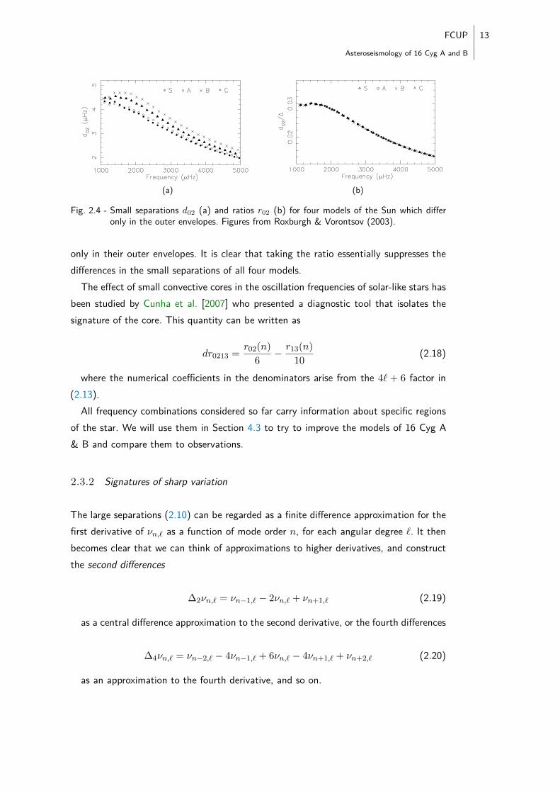
As an example, Figure 2.4 shows the small separations d02 and the ratios r02 for thedifferent models of the Sun considered by Roxburgh and Vorontsov [2003], that differ
FCUP 13
Asteroseismology of 16 Cyg A and B
216 I. W. Roxburgh and S. V. Vorontsov: Ratio of separations
Fig. 1. Large separations ∆� for ModelS and � = 0, 1, 2, 3.
Fig. 2. Scaled small separations d02/3, d13/5, d01, d10: ModelS.
being the acoustic radius of the star and c the sound speed. Thedependence on the derivative of c, which changes sign in thesolar core, suggests that the small separations give a diagnosticof the deep interior of the star. In fact the Tassoul asymptoticresult gives a poor fit both to the small separations of stellarmodels and to the observed values for the Sun. A much bet-ter fit was obtained by Roxburgh & Vorontsov (1994) using adistorted wave Born approximation.
2. Contribution of the outer layers of a star
To examine the effect of the outer layers of a star on the sep-arations we construct a set of 4 models with exactly the sameinterior structure but with different outer envelopes for r ≥ r f .That is P(r), ρ(r), Mr(r) are unchanged for r ≤ r f . One modelis modelS itself, the other three are:
Model A: P, ρ, Mr unchanged for all r but Γ1 = 5/3 for all r.Since Γ1 ≈ 5/3 for r < 0.95 R� this is almost the same as justchanging the value of Γ1 for r > 0.95 R�.
Model B: For r ≥ r f = 0.9 R� the structure of the envelope isdetermined by a linear variation of polytropic index n = n0 +
n1(r − r f ) with n continuous at r = r f . The model has a radius1 R� and mass of 1 M� and Γ1 is the same as in modelS.
Model C: For r ≥ r f = 0.72 the envelope is adiabatic withΓ1 = 5/3. This model has radius of 0.995 R�.
Fig. 3. Large separations ∆�, � = 0, 1, 2, 3, for all 4 models.
Fig. 4. Small separations d02 for all 4 models.
Fig. 5. Small separations d13 for all 4 models.
Figure 3 shows the large separations ∆� for all 4 modelsand for � = 0, 1, 2, 3. The small separations d02, d13, d01 and d10
are shown in Figs. 4–6. It is clear that the structure of the outerlayers plays a significant role in determing both large and smallseparations.
3. The ratio of small to large separations
We define the ratios ri j of small to large separations as
r02(n) =d02(n)∆1(n)
, r13(n) =d13(n)∆0(n + 1)
(7)
(a)
I. W. Roxburgh and S. V. Vorontsov: Ratio of separations 217
Fig. 6. Small separations d01, d10 for all 4 models.
Fig. 7. Ratio r02 = d02/∆1 for all 4 models.
Fig. 8. Ratio r13 = d13/∆0 for all 4 models.
r01(n) =d01(n)∆1(n)
r10(n) =d10(n)∆0(n + 1)
· (8)
Figures 7–9 show these ratios for all 4 models. As can be seenfrom these figures the ratios ri j are essentially the same for all4 models. Since the modified models are identical to the un-modified modelS in the inner layers, but differ in the outer lay-ers, this demonstrates empirically that the ratios ri j of small tolarge separations are independent of the structure of the outerlayers of a star, and therefore provide a diagnostic of the stellarinterior alone.
Fig. 9. Ratio r01 = d01/∆1, r10 = d10/∆0. for all 4 models.
4. Phase shifts and the Eigenfrequency Equation
To understand this result we introduce the concepts of phaseshifts and partial waves, and derive the Eigen-frequencyEquation of Roxburgh & Vorontsov (2000).
The equations governing the oscillations of a spherical starcan be expressed as (see e.g. Unno et al. 1979)
dξdr+
2rξ − g
c2ξ +
(1 − �(� + 1)c2
ω2r2
)p′
ρc2=�(� + 1)ω2r2
φ′ (9)
dp′
dr+g
c2p′ +
(N2 − ω2
)ρξ + ρ
dφ′
dr= 0 (10)
d2φ′
dr2+
2r
dφ′
dr− �(� + 1)
r2φ′ = 4πGρ
(p′
ρc2+
N2
gξ
)(11)
where the perturbations in radius δr, pressure δP and gravita-tional potential δΦ are decomposed in the form
δr = ξ(r)Y�meiωt, δP = p′(r)Y�meiωt, δΦ′ = φ(r)Y�meiωt (12)
with Y�m spherical harmonics and ω the angular frequency(ω = 2πν). The sound speed c, Brunt-Vaisala frequency N,and acceleration due to gravity g, are defined as
c2 = Γ1Pρ, N2 =
g2
c2
(1 − Γ1
d log ρd log P
)g =
GMr
r2· (13)
These equations are governed by boundary conditions of reg-ularity at the centre, and that at the surface the potentialφ′ matches onto the corresponding � dependent solution ofLaplace’s equation, and the wave is reflected high in the atmo-spheric layers. This reflective wave condition is often approxi-mated to the vanishing of the Lagrangian pressure perturbationp′ − ρgξ = 0 at r = R (see e.g. Unno et al. 1979; Vorontsov& Zharkov 1989).
We now define the scaled pressure perturbation ψ, andacoustic radius t, as
ψ =p′r
(ρc)1/2, t =
∫ r
0
drc· (14)
The solution ψ�(t) for a particular eigenmode is shown inFig. 10. ψ�(t) behaves like a Spherical Bessel function J�(ωt)in the interior which in turn behaves like sin(ωt − π�/2) for
(b)
Fig. 2.4 - Small separations d02 (a) and ratios r02 (b) for four models of the Sun which differonly in the outer envelopes. Figures from Roxburgh & Vorontsov (2003).
only in their outer envelopes. It is clear that taking the ratio essentially suppresses thedifferences in the small separations of all four models.The effect of small convective cores in the oscillation frequencies of solar-like stars has
been studied by Cunha et al. [2007] who presented a diagnostic tool that isolates thesignature of the core. This quantity can be written as
dr0213 =r02(n)
6− r13(n)
10(2.18)
where the numerical coefficients in the denominators arise from the 4` + 6 factor in(2.13).
All frequency combinations considered so far carry information about specific regionsof the star. We will use them in Section 4.3 to try to improve the models of 16 Cyg A& B and compare them to observations.
2.3.2 Signatures of sharp variation
The large separations (2.10) can be regarded as a finite difference approximation for thefirst derivative of νn,` as a function of mode order n, for each angular degree `. It thenbecomes clear that we can think of approximations to higher derivatives, and constructthe second differences
∆2νn,` = νn−1,` − 2νn,` + νn+1,` (2.19)
as a central difference approximation to the second derivative, or the fourth differences
∆4νn,` = νn−2,` − 4νn−1,` + 6νn,` − 4νn+1,` + νn+2,` (2.20)
as an approximation to the fourth derivative, and so on.
14 FCUPAsteroseismology of 16 Cyg A and B
The reason to consider such combinations lies in the dependence of the oscillationfrequencies on localized sharp changes in the stratification, the so called acoustic glitches.A transition in the star’s internal structure that is seismically abrupt (its radial extentis smaller than the typical wavelength of the eigenfunctions of low frequency modes)will cause a small departure from the asymptotic spacings. Each eigenfrequency will beaffected by a shift, say δνglitchn (the ` dependence is ignored), that is a periodic functionof frequency and whose characteristics depend on the location and sharpness of thetransition.The shift is very small relative to the absolute value of the frequencies but can be
enhanced by considering the second differences. To see why let us follow closely thederivation of Houdek and Gough [2007, henceforth HG07]. Assume an oscillatory signalof the form
δνglitchn = An cosxn (2.21)
where An and xn are functions of frequency. Expanding An±1 and xn±1 in a Taylorseries around An and xn (considering the frequency νn a continuous function of modeorder n) we find
xn±1 ' xn ±dνndn
dxndνn' xn ±∆ν0
dxndνn≡ xn ± a
An±1 '(
1± ν0
An
dAndνn
+ν2
0
2An
d 2Andν2n
)An ≡ (1± b+ c)An
(2.22)
where the derivatives of νn come from Eq. (2.9) at fixed ` and keeping only theleading term. From the definition of the second differences, Eq. (2.19), and writing eachfrequency as a sum of a smooth part νs and the shift δνglitchn , we obtain
∆2νn,` = ∆2νs + FAn cos(xn − δ) (2.23)
where
F = 2{
[1− (1 + c) cos a]2 + b2 sin2 a}1/2
(2.24)
and δ = δ(a, b, c). For the Sun, and in the case of the glitch that is caused by theionization of Helium near the solar surface, Houdek and Gough find a ' 1.4, b ' −0.33
and c ' 0.04 so that the oscillatory component is enhanced in the second differencesby a factor of F ' 1.7. For the glitch present at the base of the solar convection zone,a ' 4, b ' −0.10 and c ' 0.01 so that in this case, F ' 3.4.

FCUP 15
Asteroseismology of 16 Cyg A and B
We see that in the second differences, the oscillatory component dominates over thesmooth component (the latter is diminished since only second and higher order termsremain in ∆2νs) and may be easier to detect. In the next section I will study two methodsto isolate the oscillatory signals both in the frequencies and in the second differences.

3Measuring acoustic glitches
In Section 2.3.2 the second differences were introduced as probes of regions of rapidvariation in the stellar interiors. The oscillatory signal produced by these regions is presentin the oscillation frequencies and propagates to the second differences and also to othertypes of frequency combinations. In principle it can be detected both in the frequenciesand in the second differences, with the difference that in the latter the smooth componentthat results from the run of the sound speed with radius (which would be present evenin a hypothetical star with no glitches) is in part eliminated. The amplitude of the signalin the second differences is, thus, enhanced as was shown before.In order to isolate the oscillatory signal, we need to know (or assume) its functional
form and what are the parameters that describe it. In the following section I brieflydiscuss the derivation of the asymptotic expression for the signals (both at the baseof the convection zone and at the helium ionization zone) and then present the actualexpressions used to fit the signals. After that, two numerical methods used to isolate thesignals are described and finally, in Section 3.4, the results for the Sun are presented asa validation of the codes.
3.1 Nature of the signal
In order to derive an expression for the variation in frequency caused by a discontinuityin the internal structure of the star we can use a proper approximation to the adiabaticoscillation equations either in differential or integral form. The former is simpler in thecase of the base of the convection zone, but for the ionization region and to betterapproximate the frequency dependence of the amplitude of the signals a variationalprinciple yields better results [Monteiro et al., 1994, Monteiro and Thompson, 2005].Notwithstanding, if one considers the adiabatic oscillation equations in the Cowling
approximation, which can be reduced to the Schrödinger-type equation [Brodsky andVorontsov, 1993]
d2
dτ2ζ +
[ω2 − V (τ)
]ζ = 0 (3.1)
17
18 FCUPAsteroseismology of 16 Cyg A and B�� .� ��!� ��� ��������� "�������
��� ���F /0��!� �� � !�� ����� 4���� �� �������� % �4� �� �� ��� %�� L9� �M ����4� ��! � �� ! �������F � �� ! �� ��� ��� � Æ ������� �� ���
5��� ��� ���$ E$L6$ /������ ��� ���� ������ �������' �� ��)������ ���� ' 5A6 ��
�������� � ���#����' #� �� ��� ������� �� ��� �# ����� ��' �������� ���'
�������'��5A6 D �
���Z\!5A6[
���Z\!51�A�6[�� C�A�1�A�
'��5A6 D ����Z\�5A��A6[
���Z\�5A��1�A�6[ �� 1�A��A�A������
��' �������'��5A6 D �
���Z\�5A6[
���Z\�51�A�6[�� C�A�1�A�
'��5A6 D ����Z\�5A��A6[
���Z\�5A��1�A�6[ �� 1�A��A�A� $������
1��� � �� � ��� ��������' ��
\�5A6 D
�
�
��D �
�
���A D
��D �
�
���A 4 FDC E � ������
�� �# ��� � ����� � ������ � '�A $ " �' @)$ ������ �� ���������
���� 1�A� 5GD�E6 �� ���'
�����"
�����"
�'
A�A D �
�����"
�����"
��D �
' A � ����� �
7����������� ��� ��������� �� @)�$ ������ �� �����' �� ��.��� ��� ����� 0�C � �����
.�, "��� � �������� ��� ;��� ��
��� ���F '������ !�� ����� ! A�B 4��� � � ��� �� ������� � !�� �� �4� #�� ��F ����&�% ����� ��� � A"� & ���� � ��� B ��� �� �% ����� ��� � A�� & �������� ��� B,���� !�� ������ � �� � G 9, � 0! ����� � � �� � � ��� �� !�� ����� �� ��% �� ��4 �� ������
" �������� ��� �*��� � � � ����������� �� ��� ���� ��� ��� �� #� ������
������ ������� ������� �� ������ ��������� �� #���� #� ��� �������� �� �(���
������$ 7������� ��� @)$ ������ #� ��� � �������� ��� ������������ ' 5A6 #����
�� ��� ������ �� ��� ����� ���� �� � �� �� �������� D 5A6$ �� ������ �������
#� ��.� ���� �������� 5'DC6 �� ADC �� ADA�$ ,�� ��������� ������ �� ������ �
������� � � ������� �������� � ���#����' DDD�' ���$ "�� ������ �� ���)����� �'
���������� ��� ������ ������ �� ADC' ��
' 5A6 D � ���
� �
�
���D �
�
���A
� ������
#���� � �� � �������$ /������ ��� ��� ������ ������ �� ADA�' #� ����� ���
���#��� �������� �������?
���D �� D
���
A�
��
������
� ����� �� ������� ���������� � ��� 5�6�E�� �� $����� �6 � ��� ������������$
" ���������� ��� �*���� � ������������� � �������������' #� ������ �# ��������+
���� � ��� ��������� ��������$ "�� ���� �� ���� ��
D�5A6 D
�D! �� C�A 1�A
D� �� 1�A�A A� '������
#���� ��� ���� �� �� �� ��
D�5A6 D D� T Æ Æ5A�1�A�6 �����
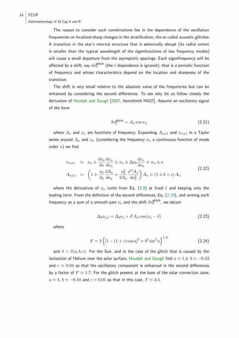
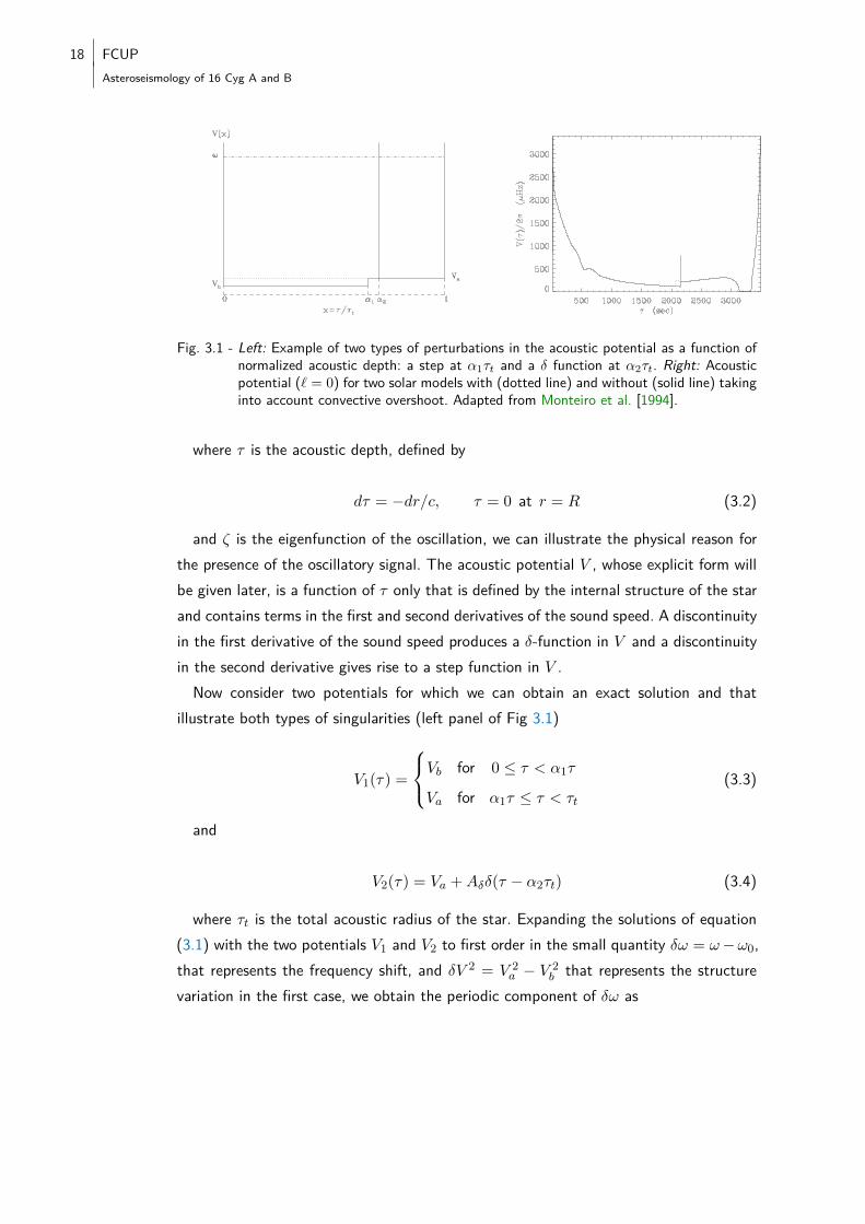
Fig. 3.1 - Left: Example of two types of perturbations in the acoustic potential as a function ofnormalized acoustic depth: a step at α1τt and a δ function at α2τt. Right: Acousticpotential (` = 0) for two solar models with (dotted line) and without (solid line) takinginto account convective overshoot. Adapted from Monteiro et al. [1994].
where τ is the acoustic depth, defined by
dτ = −dr/c, τ = 0 at r = R (3.2)
and ζ is the eigenfunction of the oscillation, we can illustrate the physical reason forthe presence of the oscillatory signal. The acoustic potential V , whose explicit form willbe given later, is a function of τ only that is defined by the internal structure of the starand contains terms in the first and second derivatives of the sound speed. A discontinuityin the first derivative of the sound speed produces a δ-function in V and a discontinuityin the second derivative gives rise to a step function in V .Now consider two potentials for which we can obtain an exact solution and that
illustrate both types of singularities (left panel of Fig 3.1)
V1(τ) =
Vb for 0 ≤ τ < α1τ
Va for α1τ ≤ τ < τt
(3.3)
and
V2(τ) = Va +Aδδ(τ − α2τt) (3.4)
where τt is the total acoustic radius of the star. Expanding the solutions of equation(3.1) with the two potentials V1 and V2 to first order in the small quantity δω = ω−ω0,that represents the frequency shift, and δV 2 = V 2
a − V 2b that represents the structure
variation in the first case, we obtain the periodic component of δω as
FCUP 19
Asteroseismology of 16 Cyg A and B
δω1 ∼δV 2
4τtω20
sin[2Λ0(α1τt)] (3.5)
and
δω2 ∼Aδ
2τtω0cos[2Λ0(α2τt)] (3.6)
for the two potentials respectively, where
Λ0(τ) =
∫ τ
0(ω2
0 − V 2a )
12dτ . (3.7)
These very simple examples already provide important insights about the frequencydependence of the amplitude of the signal and indeed do not differ much from theresults obtained for a star, in which case the toy potentials will be replaced by a morecomplicated function that depends on the interior of the star and can be determinednumerically from models (see Figure 3.1).The explicit dependence of the acoustic potential on the sound speed and its derivatives
can be written as [Vorontsov and Zharkov, 1989, Roxburgh and Vorontsov, 1994]
V 2 =N2 +c2
4
(2
r+N2
g− gc2− 1
2c2
dc2
dr
)2
− c2
d
dr
[c
(2
r+N2
g− g
c2− 1
2c2
dc2
dr
)]−4πGρ ,
(3.8)
At the base of the convection zone, g, c2 and ρ are continuous but both dc2/dr andd2c2/dr2 are discontinuous. Therefore, V can be decomposed as
V (τ) = V0(τ) +AHH(τ − τb) +Aδ1
cδ(τ − τb), (3.9)
where V0(τ) is a smooth function of τ and τ = τb is the acoustic location of the baseof the convection zone (H is the Heaviside function). Note that (3.9) has terms that areof the form (3.3) and (3.4) so that the base of the convection zone will give rise to aperiodic effect on the frequencies that is a combination of both (3.5) and (3.6).A similar analysis can be performed for the second Helium ionization region which
induces a local change to the first adiabatic exponent Γ1. The potential can be reducedto the form [Marchenkov and Vorontsov, 1991]
20 FCUPAsteroseismology of 16 Cyg A and B
V 2 ≈ g2
16 c2
[(1 + Γ1)(3− Γ1) + 2(1 + Γ1)
dΓ1
d ln p−(dΓ1
d ln p
)2
+ 4 Γ1
d2 Γ1
d(ln p)2
],
(3.10)
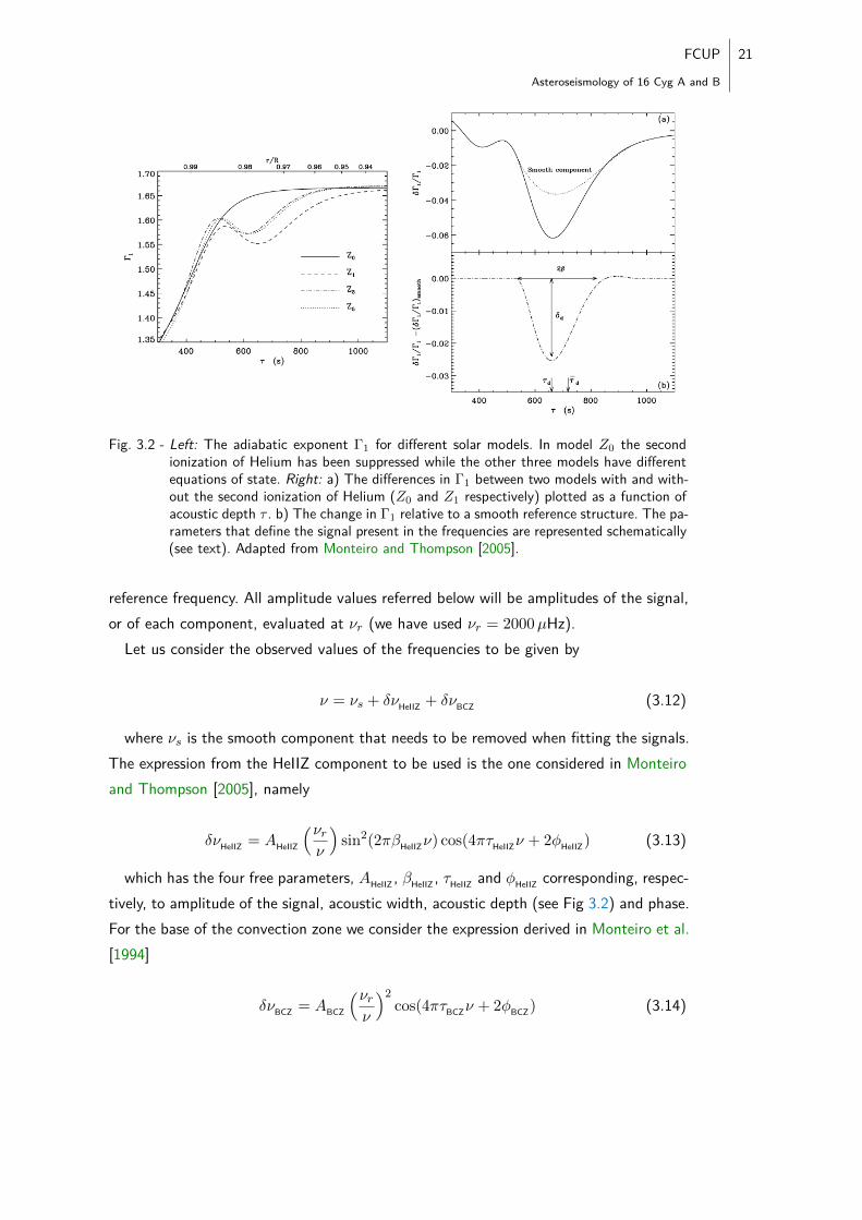
but now it is no longer feasible to consider discontinuities in the first and secondderivatives of Γ1. Instead, ionization causes a "bump" or a depression in the adiabaticexponent that extends through approximately 300 s.To model this signature we follow Monteiro and Thompson [2005] and consider a
bump of width β in acoustic depth and relative height δd. It can be shown that, relativeto a smooth model (one that has no He ionization), the frequencies will be affected bya periodic component of the form
δω ∼ A(ω) cos(2ωτ∗d + φ) (3.11)
The parameter τd (see Figure 3.2) corresponds to the acoustic depth of the middle ofthe bump, but the period of the signal that will be present on the frequencies will alsocontain a contribution from the near-surface layers, meaning that what we will be able tomeasure will not necessarily be a good estimate of this location†. Also there is no trivialrelation between the true location τd and the measured period of the signal τ∗d , althougha difference of about 200 s between the two is expected [Monteiro and Thompson, 2005].Although without extensive derivations (the interested reader is referred to the works
of, e. g., Monteiro et al. [1994] and HG07) we have demonstrated that a periodic signalin the frequencies appears as a result of sharp changes in the acoustic stratification ofstars.
3.2 Complete expressions
We have demonstrated the reasons for periodic signals to be present in the oscillationfrequencies due to the effect of the BCZ and the HeIIZ. Here we describe the exactform of the signals that will be fitted to the observed frequencies and also document thenotation used below. From now on we shall write all expressions in terms of the cyclicfrequency ν = ω/2π.Since only low degree data is available, all dependencies of the signals on ` are ignored.
A reference frequency νr will be used to normalize the amplitudes. This value does notinterfere in the fit but to compare the signal in different stars we need to use the same
†This will also affect the location of the base of the convection zone
FCUP 21
Asteroseismology of 16 Cyg A and B
2005MNRAS.361.1187M
2005MNRAS.361.1187M
Fig. 3.2 - Left: The adiabatic exponent Γ1 for different solar models. In model Z0 the secondionization of Helium has been suppressed while the other three models have differentequations of state. Right: a) The differences in Γ1 between two models with and with-out the second ionization of Helium (Z0 and Z1 respectively) plotted as a function ofacoustic depth τ . b) The change in Γ1 relative to a smooth reference structure. The pa-rameters that define the signal present in the frequencies are represented schematically(see text). Adapted from Monteiro and Thompson [2005].
reference frequency. All amplitude values referred below will be amplitudes of the signal,or of each component, evaluated at νr (we have used νr = 2000µHz).Let us consider the observed values of the frequencies to be given by
ν = νs + δνHeIIZ + δνBCZ (3.12)
where νs is the smooth component that needs to be removed when fitting the signals.The expression from the HeIIZ component to be used is the one considered in Monteiroand Thompson [2005], namely
δνHeIIZ = AHeIIZ
(νrν
)sin2(2πβHeIIZν) cos(4πτHeIIZν + 2φHeIIZ) (3.13)
which has the four free parameters, AHeIIZ , βHeIIZ , τHeIIZ and φHeIIZ corresponding, respec-tively, to amplitude of the signal, acoustic width, acoustic depth (see Fig 3.2) and phase.For the base of the convection zone we consider the expression derived in Monteiro et al.[1994]
δνBCZ = ABCZ
(νrν
)2cos(4πτBCZν + 2φBCZ) (3.14)
22 FCUPAsteroseismology of 16 Cyg A and B
with free parameters ABCZ , τBCZ and φBCZ corresponding to amplitude, acoustic depthand phase of the BCZ signal.To obtain the final expression to fit the frequencies we need in addition to specify the
smooth component νs in (3.12) but the functional form of this component is unknown.For now we will leave it unspecified but in Section 3.3 the method used to remove thisslowly varying trend will be described. The final function to fit to the frequencies is then
ν ' νs +
+ABCZ
(νrν
)2cos(4πτBCZν + 2φBCZ) +
+AHeIIZ
(νrν
)sin2(2πβHeIIZν) cos(4πτHeIIZν + 2φHeIIZ)
(3.15)
In order to derive the expressions for the second differences, the same analysis ofSection 2.3.2 can be carried out, already assuming the functional form (3.15) in thefrequencies. Guided by the frequency dependence of the asymptotic relation (2.9), we canapproximate the smooth component that is left in the second differences by a polynomial(up to third-degree) in ν−1. However, for the range of frequencies available for 16 CygA and B we find that a simpler constant term is more suitable.
The final functional form that will be fitted to the observed second differences is basedon the one used in Mazumdar et al. [2012], namely
∆2ν =
3∑
k=0
ckν−k +
+(A ∗BCZ/ν
2)
sin (4πντBCZ + 2φBCZ) +
+[A ∗HeIIZ ν exp
(−β ∗HeIIZ ν
2)]
sin (4πντHeIIZ + 2φHeIIZ)
(3.16)
with seven free‡ parameters A ∗BCZ , τBCZ , φBCZ , A ∗HeIIZ , β∗HeIIZ , τHeIIZ and φHeIIZ .
3.2.1 Expressions from Houdek & Gough
It is worth mentioning the latest results in the development of more elaborate expressionsfor the signals. Houdek and Gough [2007] performed an asymptotic analysis of the effectsof the helium ionization region and the base of the convection zone on the frequencies.They derived an expression that in principle represents the second differences more faith-fully than the expressions we are using, because their representation of the He II glitchin Γ1 and of the stratification immediately beneath the convection zone is more realistic.
‡The parameters of the polynomial smooth component (either c0−3 or just c0) are still free parametersbut they are not included in the nonlinear fit, as will be discussed in the next section.
FCUP 23
Asteroseismology of 16 Cyg A and B
The more complete expressions for the glitches come with the price of having to assumemany intermediate parameters in the derivation to have their solar (or solar calibrated)values. While correct and advantageous in the case of the Sun, many of these parametersdo not have observable values in other stars.We have carried out tests trying to fit the more realistic expressions [HG07, their Eq.
22] to the second differences of the Sun and of 16 Cyg A & B. For the Sun, the resultswere only marginally better than when fitting Eq. (3.16). For the 16 Cyg stars we werenot able to find good fits. Thus, and also supported by the fact that many parameterswould have to be set to solar values, we have not considered further these expressions.The added complexity of the functional forms does not yet seem beneficial when appliedto other stars, at least until extremely precise data (comparable to the solar data) isavailable. Also, while not the exact form prescribed by [HG07], Eq. (3.16) does containthe essential terms.
3.3 Methods to isolate the signals
This section is devoted to the description of two different numerical methods to isolateand determine the parameters of the signals given by Eq. (3.15) in the frequencies or Eq.(3.16) in the second differences.
The first method that we consider (henceforth labeled Method 1) was presented inMonteiro et al. [1994] and subsequently used to study the convective overshoot propertiesand the helium abundance of the Sun [Monteiro et al., 2000, Monteiro and Thompson,2005]. It has also been applied to other solar-type stars [Mazumdar et al., 2012].The idea is to extract the signal from the oscillation frequencies directly, by fitting a
smooth function of mode order n to the points νn,` in order to remove the slowly varyingtrend. This is done separately for each degree `, by fitting the polynomial
P`(n) =
N∑
k=1
a(`)k nk−1 (3.17)
to the N` frequencies using a least squares fit with third derivative smoothing. Theresiduals are then fitted (simultaneously for all degrees) with the expression for the signal.By iterating this procedure, the smooth function will remove variations of νn,` with scalesmuch longer than the characteristic scale of the signal without affecting it.The third derivative smoothing procedure depends on a parameter λ that basically
determines how close the polynomial P` interpolates the points or, said in another way,how smooth it is. In the original Method 1 there is an iteration over this parameter thattries to achieve the smoothest possible function that still does not interfere with the
24 FCUPAsteroseismology of 16 Cyg A and B
signals we are trying to extract (the reader is referred to Monteiro et al. [1994] for allthe details).The fact that Method 1 makes use of all the data available (does not require frequencies
of consecutive orders to construct combinations) and that it does not assume a specificfunctional form for the smooth component are its main advantages. It can, however, inits current implementation, be less robust (more dependent on starting conditions) thanother methods. This is because it uses a local minimization algorithm, meaning that theinitial conditions must be close to the true properties of the signal that is to be extracted.A second method (henceforth, Method 2) uses the second frequency differences and
fits the functional form (3.16) to the observed points ∆2νn,`. It was discussed before thatthe amplitudes of the signals are enhanced relative to the smooth component when wetake the second differences which means that the signals might be more easily extracted.The functional form of the smooth component is still not known a priori but can beapproximated by a polynomial function of frequency.Because it uses the second differences, Method 2 needs three consecutive modes of the
same degree for each point. In stars where only a small number of modes are observedwe can reach the limiting case of not having enough points to fit (or having few morepoints than free parameters). In the case of the available data for 16 Cygni though, thereare many observed modes and this is not a severe problem.Both Method 1 and 2 have been compared with each other and with other methods
to isolate the signals [Mazumdar et al., 2012] and shown to give consistent results. Inthe next sections we describe our own implementations and some improvements to bothmethods which we then use to study the acoustic glitches of 16 Cyg A & B.
3.3.1 Improving Method 1
In previous works, Method 1 has been used to isolate the contributions from the baseof the convection zone and from the helium ionization separately. This is in part dueto the difficulty in choosing a scale for the smooth function that does not affect thecharacteristics of the signals when both are considered together, but mostly is becauseof convergence problems.The value of the smoothing parameter λ determines the period of the signal that
is to be isolated. Depending on the choice of this parameter, we either ensure that thesignature associated with helium ionization is removed (with smaller values of λ) or allowit to dominate the least-squares fit (larger λ). In the latter case, the signature from thebase of the convection zone is still retained, although it may be more difficult to isolate.
FCUP 25
Asteroseismology of 16 Cyg A and B
We have tried to improve Method 1 in two complementary ways: using a global min-imization algorithm for the least-squares fit that provides robustness and independenceof initial conditions (see Section 3.3.3) and fitting both signals from the BCZ and theHeIIZ together.From tests of the parameter dependence on λ, we are able to identify a "plateau"
where both the parameters of the fit and the χ2 remain approximately unchanged in arange of values of λ. We then set this parameter to an intermediate value inside thisrange.It is important to understand why the original iteration in λ was removed. A value of
λ = 0 means the interpolating polynomial will pass through all points, effectively withoutsmoothing. Then, if λ is included in the fit as a free parameter, the best solution willalways converge to a value very close to zero, artificially making the smooth functionexplain every variation in the data. One possible solution would be to constrain thevalue of λ by, for example, penalizing the fit when the HeIIZ and BCZ signal amplitudesapproach zero. Although this is feasible and worthy of additional studies, we have nottried to implement it, in part due to our inability to specify a coherent and justifiedpenalty.As will be shown in Chapter 4, the improved Method 1 is already quite robust, even
with the arbitrariness of the setting of λ. This aspect of the fit is a shortcoming but isthe price to pay for not assuming a functional form for the smooth contribution. Thevalues used in the fits of 16 Cyg A and B were λA = 10−4 and λB = 5 × 10⁻⁴ for thetwo components respectively.
3.3.2 Implementation of Method 2
The numerical implementation of Method 2 may seem simpler, but it is important tomention some of its subtleties and to document clearly our treatment.The fit of the smooth component is carried out first and only once, so that either the
constant term c0 or the third degree polynomial is first subtracted from the data, leavingonly seven free parameters describing the properties of both signals. The choice of thedegree of the polynomial depends on the range of second differences available, althoughit will always be rather arbitrary. In the study of 16 Cygni we have only considered theconstant term, while for the Sun we used the third degree polynomial, because of thelarger range in frequencies. After removing the smooth component from the data, anon-linear least squares regression is performed by minimizing the usual χ2 quantity (ourobjective function) with the same global minimization algorithm used in the frequencies(see Section 3.3.3).
26 FCUPAsteroseismology of 16 Cyg A and B
The covariance term in the χ2 (which should be present because of correlations be-tween consecutive values of ∆2νn,`) has not been considered as it will not affect thelocation of the minimum in the parameter space but only the numerical value of theχ2 [e. g. Dodelson and Schneider, 2013]. Since we estimate the errors in the fitted pa-rameters by performing Monte Carlo simulations (and do not linearise in any way theobjective function about the minimum) our error estimates implicitly take into accountthe correlations.It is customary to consider in the fit only frequencies with errors smaller than a specific
value and/or actually remove one or more outliers. This practice is not ideal and wedo not follow it. Instead, we make our fit (more) robust against discrepant values byperforming a Iteratively Reweighted Least Squares regression [e. g. Street et al., 1988].In this process, values that deviate substantially from an initial fitted curve are given lessweight in a subsequent fit, and this is iterated until convergence (small relative variationof the parameters of the fit)§. More explicitly, we use the following algorithm:
1. Compute the inverse variance of the observations wn,` = 1/σ2n,` where σn,` are the
quoted uncertainties for the νn,` mode.2. Compute the least-squares solution weighted by wn,` .3. Compute χ2
n,` = (∆2νn,`−∆2ν)2/σ2n,`, where ∆2ν if the fitting function given by
(3.16) and ∆2νn,` the observed value of the second difference.4. Update the weights wn,` = Q/[σ2
n,` (χ2n,` +Q)] for some value of Q .
5. Go to step 2 and iterate to convergence.
The choice of Q sets the maximum effect an outlier can have on the fit. For an extremeoutlier ( χ2
n,` � Q ), the effect of that point will be down-weighted by the factor Q/χ2n,`.
For points that are well fit by the model, the weight is 1/σ2n,` as in standard weighted
least squares. A value of Q = 4 seems to work well in the context of this problem. Byusing this procedure, all the available second differences enter in the fit in a robust way.
3.3.3 Global minimization
The global minimization algorithm used here was the PIKAIA implementation of thegenetic algorithm [Charbonneau, 1995]. A genetic algorithm is an heuristic search tech-nique that incorporates the biological notion of evolution by means of natural selection. It
§Note that the parameter c0 is determined before the actual fit when we consider a constant smoothcomponent. In order to extend the robustness of the process to this parameter, we consider the medianvalue of the second differences instead of the mean, which would be the least squares solution of fittinga constant.
FCUP 27
Asteroseismology of 16 Cyg A and B
can be used to perform numerical optimization on problems characterized by ill-behavedsearch spaces and a relatively large number of free parameters.The two main advantages of using a genetic algorithm in this case are: no derivatives of
the goodness of fit function with respect to model parameters need to be computed; nostarting guesses need to be provided. In principle, and given enough time, the algorithmwill always converge to the global optimal solution, the one with the smallest residuals.
From a more technical point of view, the behavior of the genetic algorithm was setto include one-point crossover and creep mutation operators, as well as fitness-basedadjustment of the mutation rate [see Charbonneau, 2002]. In all fits, a population con-taining 50 individuals is evolved for a number of generations that can vary between 5000and 7000. These options were tuned to offer a trade off between execution speed andconvergence for our particular problem.
3.3.4 Monte Carlo simulations
After performing the fits with Methods 1 and 2 we try to estimate the errors in thesignal parameters by measuring the impact of the observational uncertainties. MonteCarlo realizations of the data are produced by affecting the frequencies (note, not thesecond differences, in Method 2) with a random error, sampled from a normal distributionwith standard deviation equal to the uncertainty quoted for the frequency. Each set ofnew frequencies is then fit in the same way as the original data.As we will see in Section 4.4, the mean and median values of the resulting distribu-
tions of the parameters are very close, and the distributions are approximately normal inmost cases, so we quote their standard deviation as the 1σ error in the correspondingparameter.
3.4 Code validation - signal in solar frequencies
It is important to validate the implementations of Methods 1 and 2 before applying themto 16 Cygni. To that end, we use low-degree solar frequencies, obtained from the BISONnetwork [Broomhall et al., 2009, cf. Table 1] and compare with results of previous works.The data used here correspond to a set of 79 modes with ` = 0 − 3 and with a meanuncertainty of 0.032µHz.Starting with the signal in the frequencies, and for comparison with Monteiro et al.
[1994] and Monteiro and Thompson [2005], we set λ = 10−6 which corresponds to thevalue used to fit the Helium component (remember that each component was fitted
28 FCUPAsteroseismology of 16 Cyg A and B
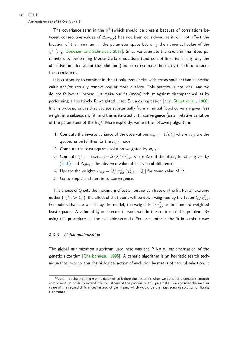
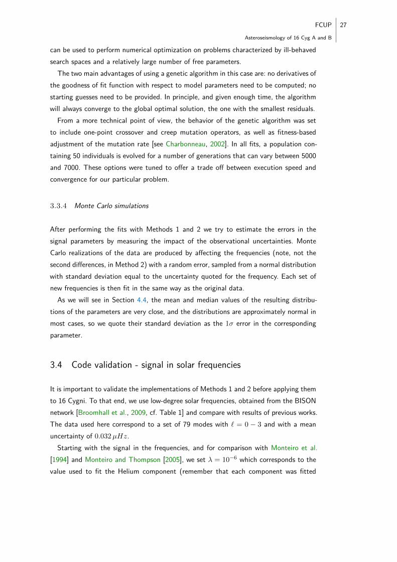
Table 3.1 - Comparison of acoustic locations in the Sun.Sun This work Previous works
δν ∆2ν δν a ∆2ν
τBCZ (s) 2270 2303 2337 2273τHeIIZ (s) 648 728 649 707a Fits to 197 modes with 5 ≤ ` ≤ 20
-2
-1
0
1
2δν
(µHz)
1000 1500 2000 2500 3000 3500 4000ν (µHz)
-2
-1
0
1
2
δν(µHz)
BCZHeIIZ
Fig. 3.3 - Top: Fit of Eq. (3.15) to the solar frequencies using the improved Method 1. The colorand symbol code is as stated in Page vii. Bottom: Individual components from theBCZ (solid line) and the HeIIZ (dashed line).
separately in previous works). The results for the locations of the glitches (τHeIIZ andτBCZ) are shown in Table 3.1 and the fit itself is in Figure 3.3.Table 3.1 shows also the results in the second differences from the fit using Method 2.
These are to be compared to the results from HG07 obtained by fitting a slightly moreelaborate form of the signal expression to GOLF and BISON data. Our fit is shown inFigure 3.4, together with the individual signal components (these should be comparedto Figure 12 from HG07).In the solar case we are not able to remove the smooth component using only a
constant term, because of the bigger range in frequencies (almost 3000µHz). The thirddegree polynomial is used but it does not interfere with the HeIIZ component.As a validation exercise, these results prove to be successful. We obtain good fits both
to the solar frequencies and second differences and the signal parameters are close tothose mentioned in the literature. Note that a perfect agreement is not to be expected
FCUP 29
Asteroseismology of 16 Cyg A and B
-4-202
∆2ν
(µHz)
1000 1500 2000 2500 3000 3500 4000ν (µHz)
-4-202
∆2ν
(µHz)
BCZHeIIZνs
Fig. 3.4 - Top: Fit of Eq. (3.16) to the solar frequencies using our implementation of Method 2.The color code is the same as in Fig (3.3) Bottom: Individual components from theBCZ (solid line) and the HeIIZ (dashed line) as well as the third degree polynomialsmooth component (dotted line).
since different frequency sets, different signal expressions and overall different methodswere used.
3.5 Amplitude magnification
As was stated before, one of the reasons to consider the second differences and attemptthe extraction of the signals in this quantity is the increased signal amplitudes. In fact,we should be more specific and say increased signal amplitudes relative to the smoothcomponent, because it is the smooth component (on top of which both signals aresuperposed) that is diminished when taking the second differences.If, and only if, both extraction methods effectively removed the same smooth function,
we would expect the resulting amplitudes to be amplified by factors close to those derivedin Section 2.3.2, approximately 3 times for the BCZ amplitude and 1.5 times for theHeIIZ amplitude (though note that those values were derived for the Sun). To test thisprediction, both the BCZ and HeIIZ signals were extracted, using both Methods, fromfrequencies of representative models of 16 Cyg A and B. The amplitudes of each signal,at a given reference frequency, were then compared between the two Methods.
30 FCUPAsteroseismology of 16 Cyg A and B
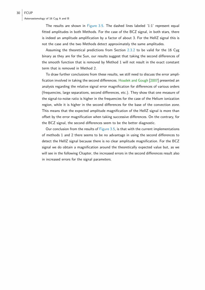
The results are shown in Figure 3.5. The dashed lines labeled ’1:1’ represent equalfitted amplitudes in both Methods. For the case of the BCZ signal, in both stars, thereis indeed an amplitude amplification by a factor of about 3. For the HeIIZ signal this isnot the case and the two Methods detect approximately the same amplitudes.Assuming the theoretical predictions from Section 2.3.2 to be valid for the 16 Cyg
binary as they are for the Sun, our results suggest that taking the second differences ofthe smooth function that is removed by Method 1 will not result in the exact constantterm that is removed in Method 2.To draw further conclusions from these results, we still need to discuss the error ampli-
fication involved in taking the second differences. Houdek and Gough [2007] presented ananalysis regarding the relative signal error magnification for differences of various orders(frequencies, large separations, second differences, etc.). They show that one measure ofthe signal-to-noise ratio is higher in the frequencies for the case of the Helium ionizationregion, while it is higher in the second differences for the base of the convection zone.This means that the expected amplitude magnification of the HeIIZ signal is more thanoffset by the error magnification when taking successive differences. On the contrary, forthe BCZ signal, the second differences seem to be the better diagnostic.Our conclusion from the results of Figure 3.5, is that with the current implementations
of methods 1 and 2 there seems to be no advantage in using the second differences todetect the HeIIZ signal because there is no clear amplitude magnification. For the BCZsignal we do obtain a magnification around the theoretically expected value but, as wewill see in the following Chapter, the increased errors in the second differences result alsoin increased errors for the signal parameters.
FCUP 31
Asteroseismology of 16 Cyg A and B
0.04 0.05 0.06 0.07 0.08
A Method 1 (µHz)
0.050.100.150.200.250.30
AM
ethod
2(µHz)
1:1
BCZ
0.35 0.45 0.55 0.65
A Method 1 (µHz)
0.35
0.45
0.55
0.65
AM
ethod
2(µHz)
1:1
HeIIZ
0.085 0.090 0.095 0.100
A Method 1 (µHz)
0.050.100.150.200.250.300.350.40
AM
ethod
2(µHz)
1:1
BCZ
0.9 1.0 1.1 1.2 1.3 1.4
A Method 1 (µHz)
0.91.01.11.21.31.4
AM
ethod
2(µHz)
1:1
HeIIZ
Fig. 3.5 - Amplitudes of the BCZ and HeIIZ signals obtained with Method 2 versus those obtainedwith Method 1 for 16 Cyg A (left) and B (right) using frequencies of representativemodels. The dashed line represents a one-to-one relation.

4The solar-type stars 16 Cyg A & B
This chapter presents the analysis of the asteroseismic data of 16 Cyg A & B. It focuseson the modeling of both stars using the MESA code and in the detection and charac-terization of features related to the acoustic glitches, exploring the methods discussed inChapter 3.A discussion of the basic properties of both stars and of the 16 Cygni system as a whole
(Section 4.1) is followed by a description of the available data from the Kepler spacetelescope. The observed oscillation frequencies are listed and will be used in the followingsections for the asteroseismic analysis of these two sources. Section 4.3 gives the resultsof the stellar modeling and Section 4.4 shows results regarding the acoustic glitches.Finally in Section 4.5 a preliminary calibration of the surface helium abundance usingthe glitch parameters is presented.
4.1 Stellar properties
The two stars 16 Cyg A (HD 186408) and B (HD 186427) are a common proper-motionpair of solar analogs with spectral types G1.5V and G3V, respectively [Schuler et al.,2011]. Global stellar parameters and abundances have been derived by Ramírez et al.[2009] and recently White et al. [2013] combined interferometric observations fromCHARA with parallaxes from Hipparcos and spectrophotometric bolometric fluxes toderive additional constraints. Both stars are physically very similar. Some relevant prop-erties of the stars are summarized in Table 4.1. Their observed position in the HR diagramis shown in Figure 4.1, together with model tracks from Marques et al. [2008]. Note thatthe chemical composition of the models in these tracks is neither calibrated to the Sunnor to 16 Cyg so that the only insight coming from Figure 4.1 is to expect 16 Cyg A &B to be more evolved than the Sun.One important difference between the two components is the presence of a 1.5 MJup
planet in an eccentric orbit (e = 0.63) around 16 Cyg B [Cochran et al., 1997]. An Mdwarf binary companion of 16 Cyg A, with a separation of ∼ 3′′ was also detected [Turneret al., 2001, Patience et al., 2002], and later confirmed by Raghavan et al. [2006].
33
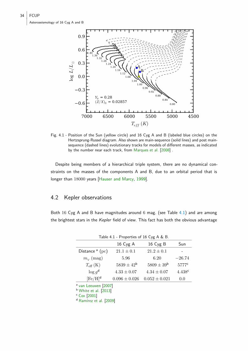
34 FCUPAsteroseismology of 16 Cyg A and B
450050005500600065007000Teff (K)
0.6
0.3
0.0
0.3
0.6
0.9
logL/L¯
0.800.84
0.880.92
0.961.00
1.041.08
1.121.16
1.201.24
1.281.32
1.361.40
AB
Y0 = 0.28(Z/X)0 = 0.02857
Fig. 4.1 - Position of the Sun (yellow circle) and 16 Cyg A and B (labeled blue circles) on theHertzsprung-Russel diagram. Also shown are main-sequence (solid lines) and post main-sequence (dashed lines) evolutionary tracks for models of different masses, as indicatedby the number near each track, from Marques et al. [2008] .
Despite being members of a hierarchical triple system, there are no dynamical con-straints on the masses of the components A and B, due to an orbital period that islonger than 18000 years [Hauser and Marcy, 1999].
4.2 Kepler observations
Both 16 Cyg A and B have magnitudes around 6 mag. (see Table 4.1) and are amongthe brightest stars in the Kepler field of view. This fact has both the obvious advantage
Table 4.1 - Properties of 16 Cyg A & B.16 Cyg A 16 Cyg B Sun
Distance a (pc) 21.1± 0.1 21.2± 0.1 -mV (mag) 5.96 6.20 −26.74
Teff (K) 5839± 42b 5809± 39b 5777c
log gd 4.33± 0.07 4.34± 0.07 4.438c
[Fe/H]d 0.096± 0.026 0.052± 0.021 0.0a van Leeuwen [2007]b White et al. [2013]c Cox [2001]d Ramírez et al. [2009]
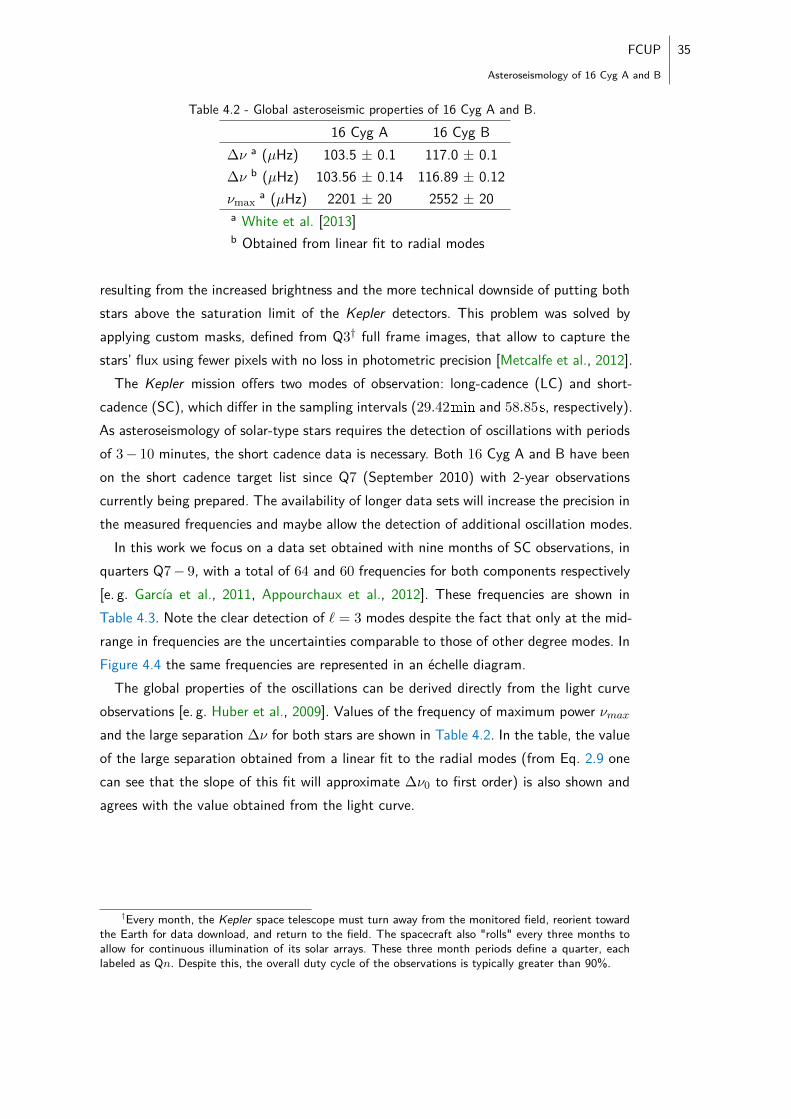
FCUP 35
Asteroseismology of 16 Cyg A and B
Table 4.2 - Global asteroseismic properties of 16 Cyg A and B.16 Cyg A 16 Cyg B
∆ν a (µHz) 103.5 ± 0.1 117.0 ± 0.1∆ν b (µHz) 103.56 ± 0.14 116.89 ± 0.12νmax
a (µHz) 2201 ± 20 2552 ± 20a White et al. [2013]b Obtained from linear fit to radial modes
resulting from the increased brightness and the more technical downside of putting bothstars above the saturation limit of the Kepler detectors. This problem was solved byapplying custom masks, defined from Q3† full frame images, that allow to capture thestars’ flux using fewer pixels with no loss in photometric precision [Metcalfe et al., 2012].The Kepler mission offers two modes of observation: long-cadence (LC) and short-
cadence (SC), which differ in the sampling intervals (29.42min and 58.85s, respectively).As asteroseismology of solar-type stars requires the detection of oscillations with periodsof 3− 10 minutes, the short cadence data is necessary. Both 16 Cyg A and B have beenon the short cadence target list since Q7 (September 2010) with 2-year observationscurrently being prepared. The availability of longer data sets will increase the precision inthe measured frequencies and maybe allow the detection of additional oscillation modes.In this work we focus on a data set obtained with nine months of SC observations, in
quarters Q7− 9, with a total of 64 and 60 frequencies for both components respectively[e. g. García et al., 2011, Appourchaux et al., 2012]. These frequencies are shown inTable 4.3. Note the clear detection of ` = 3 modes despite the fact that only at the mid-range in frequencies are the uncertainties comparable to those of other degree modes. InFigure 4.4 the same frequencies are represented in an échelle diagram.The global properties of the oscillations can be derived directly from the light curve
observations [e. g. Huber et al., 2009]. Values of the frequency of maximum power νmaxand the large separation ∆ν for both stars are shown in Table 4.2. In the table, the valueof the large separation obtained from a linear fit to the radial modes (from Eq. 2.9 onecan see that the slope of this fit will approximate ∆ν0 to first order) is also shown andagrees with the value obtained from the light curve.
†Every month, the Kepler space telescope must turn away from the monitored field, reorient towardthe Earth for data download, and return to the field. The spacecraft also "rolls" every three months toallow for continuous illumination of its solar arrays. These three month periods define a quarter, eachlabeled as Qn. Despite this, the overall duty cycle of the observations is typically greater than 90%.
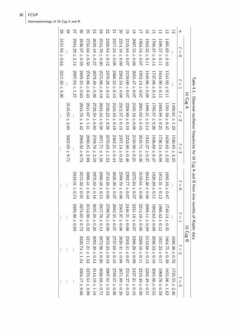
36 FCUPAsteroseismology of 16 Cyg A and B
Table4.3
-Observed
oscillationfrequenciesfor16
CygAand
Bfrom
ninemonthsofK
eplerdata.
16Cyg
A16
CygB
n`
=0
`=
1`
=2
`=
3`
=0
`=
1`
=2
`=
3
12...
...1490.01±
1.291530.85±
4.25...
...1686.36±
0.76
1735.55±2.46
1314
95.0
2±0.1
01541.9
2±0.11
1591.50±0.45
1629.82±2.22
1695.10±0.87
1749.14±0.35
1804.75±0.39
1855.06±1.62
14
1598.57±
0.11164
4.90±0.15
1693.88±0.25
1736.54±0.88
1812.31±0.12
1866.42±0.12
1921.23±0.17
1969.76±0.59
1517
00.8
7±0.1
41747.0
6±0.1
31795.87±
0.261836.69±
0.47
1928.89±0.11
1982.63±0.09
2036.53±0.18
2085.86±0.55
16
1802.22±
0.11184
8.96±0.08
1898.21±0.14
1942.27±0.37
2044.36±0.08
2098.11±0.09
2152.66±0.13
2202.49±0.51
1719
04.5
4±0.0
71952.1
3±0.0
72001.62±
0.102045.71±
0.26
2159.61±0.09
2214.10±0.08
2269.10±0.11
2319.40±0.30
18
2007.55±
0.08205
5.47±0.07
2105.16±0.08
2150.90±0.21
2275.94±0.07
2331.18±0.07
2386.26±0.09
2437.21±0.18
1921
10.8
4±0.0
72159.0
0±0.0
72208.80±
0.102253.80±
0.46
2392.77±0.07
2448.21±0.06
2503.41±0.07
2554.27±0.19
20
2214.16±
0.09226
2.53±0.08
2312.57±0.13
2357.14±0.23
2509.70±0.06
2565.37±0.06
2620.41±0.08
2671.89±0.20
2123
17.2
4±0.0
82366.2
2±0.1
02416.10±
0.192462.21±
0.44
2626.39±0.07
2682.35±0.07
2737.68±0.10
2789.57±0.36
22
2420.84±
0.12247
0.28±0.13
2520.22±0.28
2570.63±1.23
2743.38±0.08
2799.70±0.08
2855.23±0.19
2907.01±0.53
2325
24.7
0±0.2
02575.0
6±0.1
92624.34±
0.382671.71±
1.28
2860.48±0.15
2917.76±0.14
2972.96±0.26
3026.60±0.71
24
2629.18±
0.27267
9.49±0.26
2729.50±0.80
2769.76±2.59
2978.33±0.16
3035.48±0.20
3092.39±0.54
3144.19±1.18
2527
34.0
4±0.5
02784.8
6±0.4
32841.07±
1.412880.85±
2.89
3096.41±0.44
3154.00±0.32
3211.21±1.53
3270.51±3.99
26
2836.97±
0.59288
9.25±0.63
2944.76±4.42
2983.32±6.73
3215.32±0.91
3274.65±0.72
3326.74±1.54
3384.17±9.66
2729
44.2
9±2.1
42997.9
4±1.2
7...
...3333.01±
0.74
3393.30±0.63
......
28...
...3145.65±
2.003202.02±
9.71...
......
...29
3151.9
4±0.6
43211.3
0±3.3
6...
......
......
...
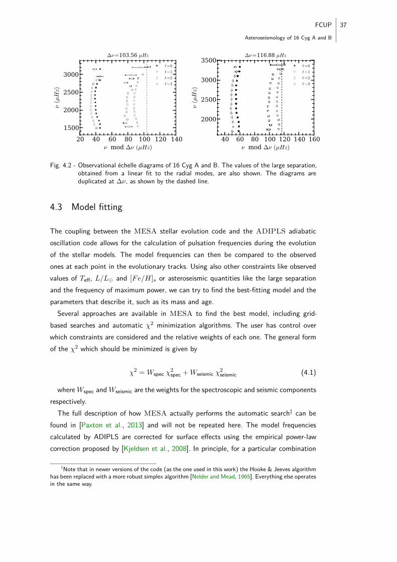
FCUP 37
Asteroseismology of 16 Cyg A and B
20 40 60 80 100 120 140ν mod ∆ν (µHz)
1500
2000
2500
3000
ν(µHz)
∆ν=103.56 µHz
`=0
`=1
`=2
`=3
40 60 80 100 120 140 160ν mod ∆ν (µHz)
2000
2500
3000
3500
ν(µHz)
∆ν=116.88 µHz
`=0
`=1
`=2
`=3
Fig. 4.2 - Observational échelle diagrams of 16 Cyg A and B. The values of the large separation,obtained from a linear fit to the radial modes, are also shown. The diagrams areduplicated at ∆ν, as shown by the dashed line.
4.3 Model fitting
The coupling between the MESA stellar evolution code and the ADIPLS adiabaticoscillation code allows for the calculation of pulsation frequencies during the evolutionof the stellar models. The model frequencies can then be compared to the observedones at each point in the evolutionary tracks. Using also other constraints like observedvalues of Teff, L/L� and [Fe/H]s or asteroseismic quantities like the large separationand the frequency of maximum power, we can try to find the best-fitting model and theparameters that describe it, such as its mass and age.Several approaches are available in MESA to find the best model, including grid-
based searches and automatic χ2 minimization algorithms. The user has control overwhich constraints are considered and the relative weights of each one. The general formof the χ2 which should be minimized is given by
χ2 = Wspec χ2spec +Wseismic χ
2seismic (4.1)
whereWspec andWseismic are the weights for the spectroscopic and seismic componentsrespectively.The full description of how MESA actually performs the automatic search‡ can be
found in [Paxton et al., 2013] and will not be repeated here. The model frequenciescalculated by ADIPLS are corrected for surface effects using the empirical power-lawcorrection proposed by [Kjeldsen et al., 2008]. In principle, for a particular combination
‡Note that in newer versions of the code (as the one used in this work) the Hooke & Jeeves algorithmhas been replaced with a more robust simplex algorithm [Nelder and Mead, 1965]. Everything else operatesin the same way.
38 FCUPAsteroseismology of 16 Cyg A and B
of evolution and pulsation codes the power-law exponent (usually denoted b) should bedetermined from a solar calibration which would define the physics to be used in themodels. However, it has been shown that variations of b do not affect the mean densityof the models [Kjeldsen et al., 2008] and one unique value can be used to model all stars.Therefore we set this parameter to the standard value of 4.9 that was obtained in theoriginal work. The seismic component of the χ2 which contains the frequencies has theform described in [Brandão et al., 2011, eq. (11)].The physics included in each model is the following: the equation of state tables
are based on the 2005 update of the OPAL EOS tables [Rogers and Nayfonov, 2002],radiative opacities are taken from OPAL [Iglesias and Rogers, 1993, 1996] and [Fergusonet al., 2005], and nuclear reaction rates from NACRE [Angulo et al., 1999]. Convectionis treated with the standard mixing-length theory as presented in [Cox and Giuli, 1968],without overshoot. Particle diffusion and gravitational settling are included using themethod and coefficients of [Thoul et al., 1994]. Each physics module is described inmore detail in [Paxton et al., 2011] and the full list of input parameters used in our workcan be found at the url https://www.astro.up.pt/~jfaria/msc-thesis for futurereference and reproducibility.It is important to also describe recent updates to the code that allow the frequency
ratios described in Section 2.3.1 to be included in the fitting process. For each modelin the evolutionary tracks, the uncorrected model frequencies§ are used to obtain thecurrent values of the model ratios which are then compared to the observed ones. Thisis included in the seismic component of the χ2 with an individual weight that is alsouser-defined. We only include the r02 and r010 ratios.Note that by calculating the ratios with frequencies to which the surface correction has
not yet been applied, we are removing the undesired bias that results from this ad-hoccorrection. Also note that we do not take into account the correlations present in ther010 ratios. To do that we would have to include the covariance matrix in the χ2. Theposition of the minimum in the parameter space (the parameters of the best model) willnot change because of this.In principle, by including in the fit only the frequency ratios and not the frequencies
themselves, the converged model would be a better representation of the interior ofthe star, less biased by the incorrect modelling of the near-surface layers and by theempirical surface correction [Silva Aguirre et al., 2013]. In practice, the ratios alonecannot guarantee a clear identification of the mode degrees and so at least one radial
§Actually, in the default version of the code available for download, the corrected frequencies areused to calculate the ratios. We believe that using the frequencies before applying the surface correctionis more accurate and more inline with our justification for using the ratios. A custom version of MESAthat uses uncorrected frequencies was thus used in this work (the changes will be subject to communityreview to be included in the main version).
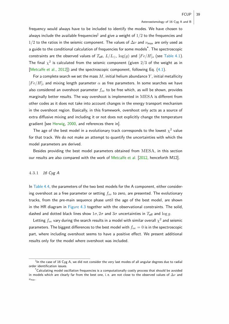
FCUP 39
Asteroseismology of 16 Cyg A and B
frequency would always have to be included to identify the modes. We have chosen toalways include the available frequencies‖ and give a weight of 1/2 to the frequencies and1/2 to the ratios in the seismic component. The values of ∆ν and νmax are only used asa guide to the conditional calculation of frequencies for some models*. The spectroscopicconstraints are the observed values of Teff, L/L�, log(g) and [Fe/H]s (see Table 4.1).The final χ2 is calculated from the seismic component (given 2/3 of the weight as in[Metcalfe et al., 2012]) and the spectroscopic component, following Eq. (4.1).For a complete search we set the massM , initial helium abundance Y , initial metallicity
[Fe/H]i and mixing length parameter α as free parameters. In some searches we havealso considered an overshoot parameter fov to be free which, as will be shown, providesmarginally better results. The way overshoot is implemented in MESA is different fromother codes as it does not take into account changes in the energy transport mechanismin the overshoot region. Basically, in this framework, overshoot only acts as a source ofextra diffusive mixing and including it or not does not explicitly change the temperaturegradient [see Herwig, 2000, and references there in].The age of the best model in a evolutionary track corresponds to the lowest χ2 value
for that track. We do not make an attempt to quantify the uncertainties with which themodel parameters are derived.Besides providing the best model parameters obtained from MESA, in this section
our results are also compared with the work of Metcalfe et al. [2012, henceforth M12].
4.3.1 16 Cyg A
In Table 4.4, the parameters of the two best models for the A component, either consider-ing overshoot as a free parameter or setting fov to zero, are presented. The evolutionarytracks, from the pre-main sequence phase until the age of the best model, are shownin the HR diagram in Figure 4.3 together with the observational constraints. The solid,dashed and dotted black lines show 1σ, 2σ and 3σ uncertainties in Teff and log g.Letting fov vary during the search results in a model with similar overall χ2 and seismic
parameters. The biggest differences to the best model with fov = 0 is in the spectroscopicpart, where including overshoot seems to have a positive effect. We present additionalresults only for the model where overshoot was included.
‖In the case of 16 Cyg A, we did not consider the very last modes of all angular degrees due to radialorder identification issues.
*Calculating model oscillation frequencies is a computationally costly process that should be avoidedin models which are clearly far from the best one, i. e. are not close to the observed values of ∆ν andνmax.
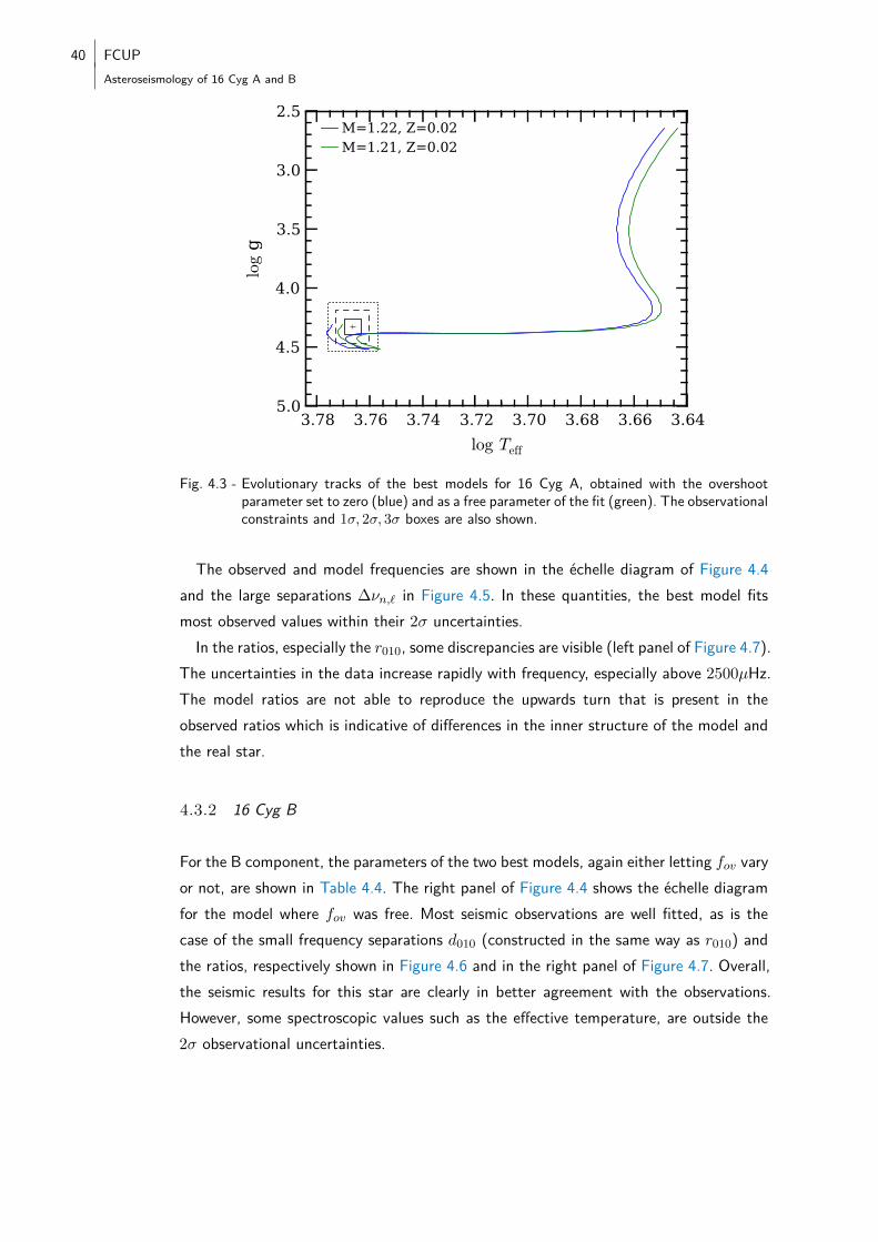
40 FCUPAsteroseismology of 16 Cyg A and B
3.643.663.683.703.723.743.763.78log Teff
2.5
3.0
3.5
4.0
4.5
5.0
log
g
M=1.22, Z=0.02M=1.21, Z=0.02
Fig. 4.3 - Evolutionary tracks of the best models for 16 Cyg A, obtained with the overshootparameter set to zero (blue) and as a free parameter of the fit (green). The observationalconstraints and 1σ, 2σ, 3σ boxes are also shown.
The observed and model frequencies are shown in the échelle diagram of Figure 4.4and the large separations ∆νn,` in Figure 4.5. In these quantities, the best model fitsmost observed values within their 2σ uncertainties.In the ratios, especially the r010, some discrepancies are visible (left panel of Figure 4.7).
The uncertainties in the data increase rapidly with frequency, especially above 2500µHz.The model ratios are not able to reproduce the upwards turn that is present in theobserved ratios which is indicative of differences in the inner structure of the model andthe real star.
4.3.2 16 Cyg B
For the B component, the parameters of the two best models, again either letting fov varyor not, are shown in Table 4.4. The right panel of Figure 4.4 shows the échelle diagramfor the model where fov was free. Most seismic observations are well fitted, as is thecase of the small frequency separations d010 (constructed in the same way as r010) andthe ratios, respectively shown in Figure 4.6 and in the right panel of Figure 4.7. Overall,the seismic results for this star are clearly in better agreement with the observations.However, some spectroscopic values such as the effective temperature, are outside the2σ observational uncertainties.
FCUP 41
Asteroseismology of 16 Cyg A and B
4.3.3 Comparison with previous results
In Table 4.4 are also shown the parameters derived by [M12] for both stars. In that workboth stars were modelled by fitting the individual frequencies obtained from three monthsof Kepler data and the spectroscopic constraints from Ramírez et al. [2009]. Instead ofusing just one stellar evolution code and fitting method, a total of seven models wereobtained for each star. Each of these models was calculated with a different numericalcode, and includes slightly different input physics and assumptions. An ensemble result(average of all the models) was also calculated.
Our best model results are close to the ensemble average in the case of 16 Cyg B,but for the A component, they do not compare as well. Our models of 16 Cyg A aremore massive and have a bigger radii (and thus a younger age to be able to match theobserved large separation).There are many possible explanations for these differences. This is one of the first times
MESA is being used in the context of asteroseismic model fitting. From the analysis in[M12], it is obvious that a simple change of the stellar evolution code, even with similarfitting methods, can impact the resulting best parameters. In this regard, we should alsonote that MESA’s χ2 minimization algorithms are not global and thus are more proneto getting stuck in local minima than, for example, the genetic algorithm used in AMP6.In addition, we have considered a longer time series of Kepler data and have included thefrequency ratios in the analysis. We made an effort to include every available frequency,despite its observational error.In our analysis, the chemical composition and age of one component was not con-
strained to match the other’s. While we do obtain some agreement in the ages, especiallywhen we let fov vary, the initial Helium abundances of the models are somewhat differ-ent. Assuming a common origin for the binary system, these parameters should agreebetween the components, which raises one important question: should we expect thebest models to agree with each other in stellar ages and initial chemical compositions orshould we force this agreement, based on a priori assumptions about the binary system?It is possible to devise a process where both components of the binary undergo seismicfitting at the same time, using MESA’s ability to evolve more than one stellar model atthe same time. This is something that should be further explored in the future for thecases of 16 Cyg as well as other binary systems.
6Of course a global minimization algorithm requires many more function evaluations (stellar evolutiontracks) thus involving a much greater computational cost.
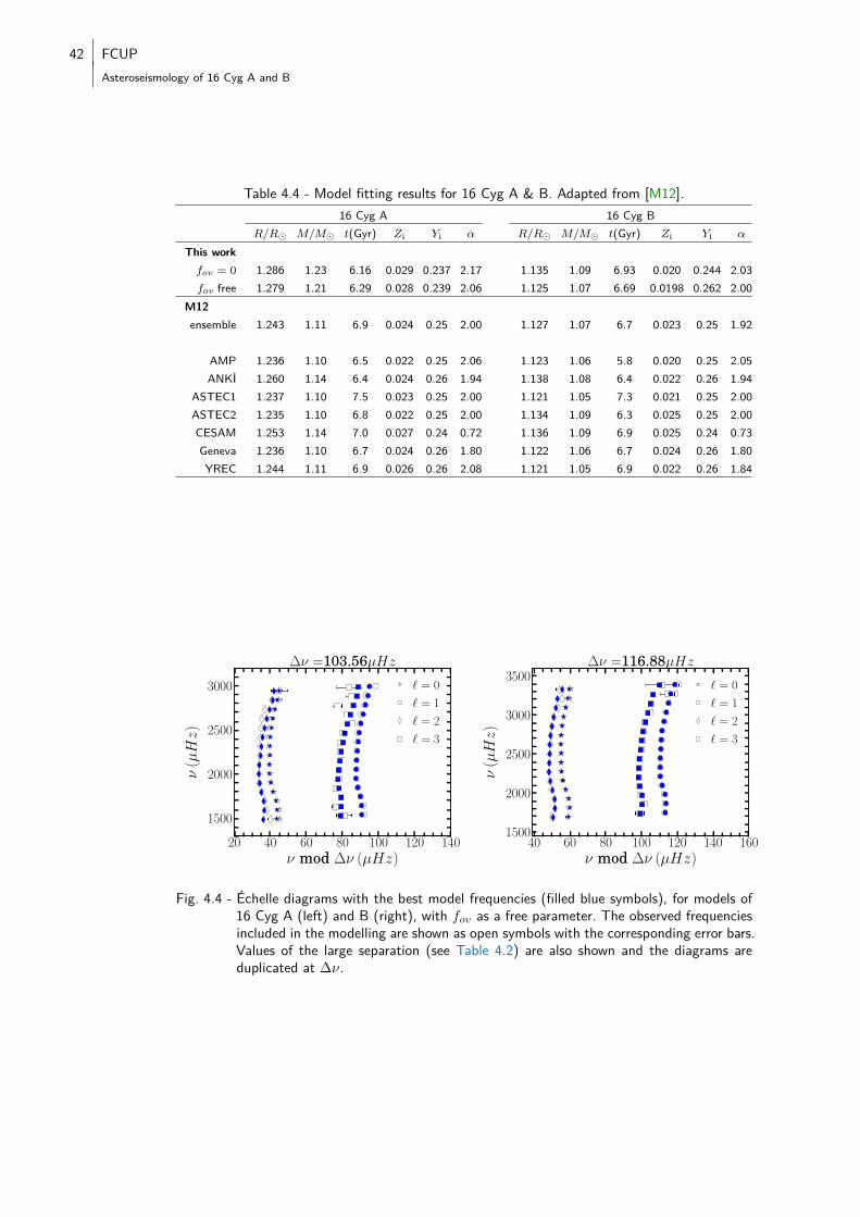
42 FCUPAsteroseismology of 16 Cyg A and B
Table 4.4 - Model fitting results for 16 Cyg A & B. Adapted from [M12].16 Cyg A 16 Cyg B
R/R� M/M� t(Gyr) Zi Yi α R/R� M/M� t(Gyr) Zi Yi α
This workfov = 0 1.286 1.23 6.16 0.029 0.237 2.17 1.135 1.09 6.93 0.020 0.244 2.03fov free 1.279 1.21 6.29 0.028 0.239 2.06 1.125 1.07 6.69 0.0198 0.262 2.00
M12ensemble 1.243 1.11 6.9 0.024 0.25 2.00 1.127 1.07 6.7 0.023 0.25 1.92
AMP 1.236 1.10 6.5 0.022 0.25 2.06 1.123 1.06 5.8 0.020 0.25 2.05ANKİ 1.260 1.14 6.4 0.024 0.26 1.94 1.138 1.08 6.4 0.022 0.26 1.94
ASTEC1 1.237 1.10 7.5 0.023 0.25 2.00 1.121 1.05 7.3 0.021 0.25 2.00ASTEC2 1.235 1.10 6.8 0.022 0.25 2.00 1.134 1.09 6.3 0.025 0.25 2.00CESAM 1.253 1.14 7.0 0.027 0.24 0.72 1.136 1.09 6.9 0.025 0.24 0.73Geneva 1.236 1.10 6.7 0.024 0.26 1.80 1.122 1.06 6.7 0.024 0.26 1.80YREC 1.244 1.11 6.9 0.026 0.26 2.08 1.121 1.05 6.9 0.022 0.26 1.84
20 40 60 80 100 120 140ν mod ∆ν (µHz)
1500
2000
2500
3000
ν(µHz)
∆ν =103.56µHz` = 0
` = 1
` = 2
` = 3
40 60 80 100 120 140 160ν mod ∆ν (µHz)
1500
2000
2500
3000
3500
ν(µHz)
∆ν =116.88µHz` = 0
` = 1
` = 2
` = 3
Fig. 4.4 - Échelle diagrams with the best model frequencies (filled blue symbols), for models of16 Cyg A (left) and B (right), with fov as a free parameter. The observed frequenciesincluded in the modelling are shown as open symbols with the corresponding error bars.Values of the large separation (see Table 4.2) are also shown and the diagrams areduplicated at ∆ν.
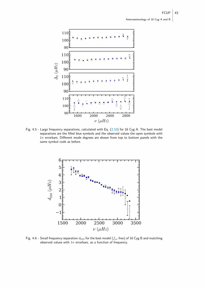
FCUP 43
Asteroseismology of 16 Cyg A and B
90
100
110
90
100
110
90
100
110
1600 2000 2400 2800ν (µHz)
90
100
110
∆`(µHz)
Fig. 4.5 - Large frequency separations, calculated with Eq. (2.10) for 16 Cyg A. The best modelseparations are the filled blue symbols and the observed values the open symbols with1σ errorbars. Different mode degrees are shown from top to bottom panels with thesame symbol code as before.
1500 2000 2500 3000 3500ν (µHz)
10123456
d01
0(µHz)
Fig. 4.6 - Small frequency separation d010 for the best model (fov free) of 16 Cyg B and matchingobserved values with 1σ errorbars, as a function of frequency.
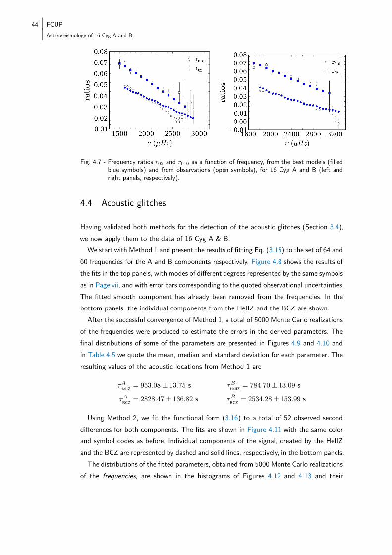
44 FCUPAsteroseismology of 16 Cyg A and B
Fig. 4.7 - Frequency ratios r02 and r010 as a function of frequency, from the best models (filledblue symbols) and from observations (open symbols), for 16 Cyg A and B (left andright panels, respectively).
4.4 Acoustic glitches
Having validated both methods for the detection of the acoustic glitches (Section 3.4),we now apply them to the data of 16 Cyg A & B.
We start with Method 1 and present the results of fitting Eq. (3.15) to the set of 64 and60 frequencies for the A and B components respectively. Figure 4.8 shows the results ofthe fits in the top panels, with modes of different degrees represented by the same symbolsas in Page vii, and with error bars corresponding to the quoted observational uncertainties.The fitted smooth component has already been removed from the frequencies. In thebottom panels, the individual components from the HeIIZ and the BCZ are shown.After the successful convergence of Method 1, a total of 5000 Monte Carlo realizations
of the frequencies were produced to estimate the errors in the derived parameters. Thefinal distributions of some of the parameters are presented in Figures 4.9 and 4.10 andin Table 4.5 we quote the mean, median and standard deviation for each parameter. Theresulting values of the acoustic locations from Method 1 are
τAHeIIZ = 953.08± 13.75 s τBHeIIZ = 784.70± 13.09 s
τABCZ = 2828.47± 136.82 s τBBCZ = 2534.28± 153.99 s
Using Method 2, we fit the functional form (3.16) to a total of 52 observed seconddifferences for both components. The fits are shown in Figure 4.11 with the same colorand symbol codes as before. Individual components of the signal, created by the HeIIZand the BCZ are represented by dashed and solid lines, respectively, in the bottom panels.The distributions of the fitted parameters, obtained from 5000 Monte Carlo realizations
of the frequencies, are shown in the histograms of Figures 4.12 and 4.13 and their
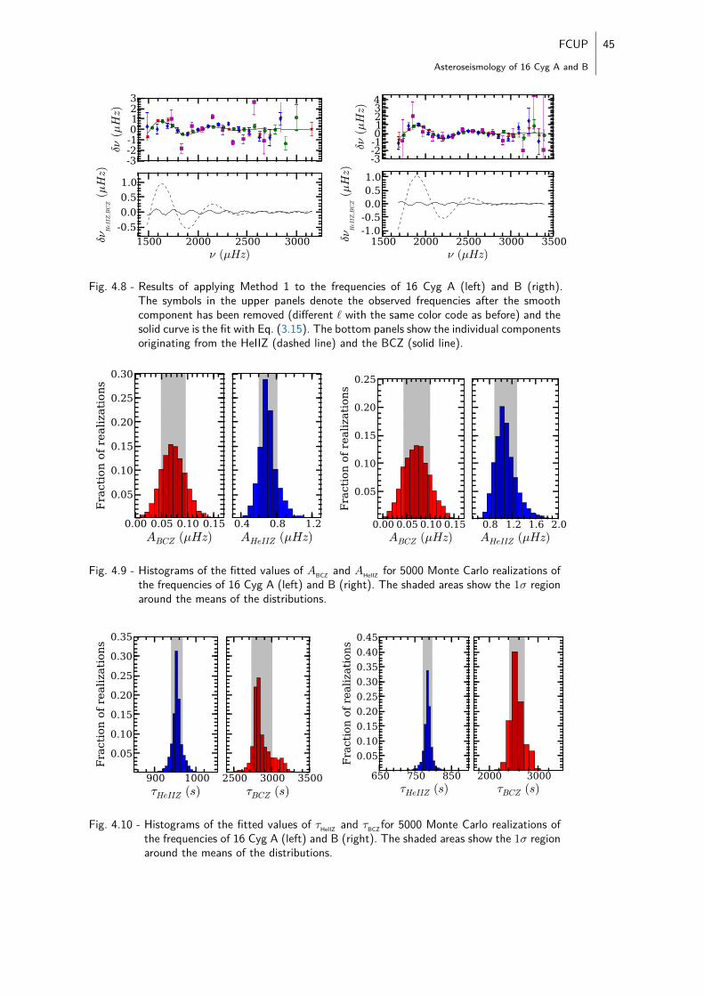
FCUP 45
Asteroseismology of 16 Cyg A and B
-3-2-10123
δν(µHz)
1500 2000 2500 3000ν (µHz)
-0.50.00.51.0
δνHeIIZ,BCZ
(µHz)
-3-2-101234
δν(µHz)
1500 2000 2500 3000 3500ν (µHz)
-1.0-0.50.00.51.0
δνHeIIZ,BCZ
(µHz)
Fig. 4.8 - Results of applying Method 1 to the frequencies of 16 Cyg A (left) and B (rigth).The symbols in the upper panels denote the observed frequencies after the smoothcomponent has been removed (different ` with the same color code as before) and thesolid curve is the fit with Eq. (3.15). The bottom panels show the individual componentsoriginating from the HeIIZ (dashed line) and the BCZ (solid line).
0.00 0.05 0.10 0.15ABCZ (µHz)
0.05
0.10
0.15
0.20
0.25
0.30
Fra
ctio
n o
f re
ali
zati
on
s
0.4 0.8 1.2AHeIIZ (µHz)
0.00 0.05 0.10 0.15ABCZ (µHz)
0.05
0.10
0.15
0.20
0.25
Fra
ctio
n o
f re
ali
zati
on
s
0.8 1.2 1.6 2.0AHeIIZ (µHz)
Fig. 4.9 - Histograms of the fitted values of ABCZ and AHeIIZ for 5000 Monte Carlo realizations ofthe frequencies of 16 Cyg A (left) and B (right). The shaded areas show the 1σ regionaround the means of the distributions.
900 1000τHeIIZ (s)
0.05
0.10
0.15
0.20
0.25
0.30
0.35
Fra
ctio
n o
f re
ali
zati
on
s
2500 3000 3500τBCZ (s)
650 750 850τHeIIZ (s)
0.05
0.10
0.15
0.20
0.25
0.30
0.35
0.40
0.45
Fra
ctio
n o
f re
ali
zati
on
s
2000 3000τBCZ (s)
Fig. 4.10 - Histograms of the fitted values of τHeIIZ and τBCZ for 5000 Monte Carlo realizations ofthe frequencies of 16 Cyg A (left) and B (right). The shaded areas show the 1σ regionaround the means of the distributions.
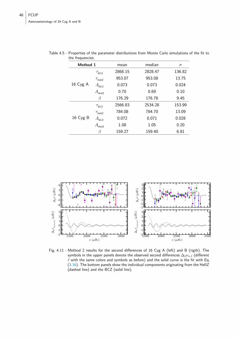
46 FCUPAsteroseismology of 16 Cyg A and B
Table 4.5 - Properties of the parameter distributions from Monte Carlo simulations of the fit tothe frequencies.
Method 1 mean median σ
16 Cyg A
τBCZ 2868.15 2828.47 136.82τHeIIZ 953.07 953.08 13.75ABCZ 0.073 0.073 0.024AHeIIZ 0.70 0.69 0.10β 176.29 176.78 9.45
16 Cyg B
τBCZ 2566.83 2534.28 153.99τHeIIZ 784.08 784.70 13.09ABCZ 0.072 0.071 0.028AHeIIZ 1.08 1.05 0.20β 159.27 159.40 6.81
-4
-2
0
2
4
∆2ν
(µHz)
1500 2000 2500 3000ν (µHz)
-2-10123
∆2ν H
eIIZ,BCZ
(µHz)
-3-2-10123
∆2ν
(µHz)
1500 2000 2500 3000 3500ν (µHz)
-2-10123
∆2ν H
eIIZ,BCZ
(µHz)
Fig. 4.11 - Method 2 results for the second differences of 16 Cyg A (left) and B (rigth). Thesymbols in the upper panels denote the observed second differences ∆2νn,` (different` with the same colors and symbols as before) and the solid curve is the fit with Eq.(3.16). The bottom panels show the individual components originating from the HeIIZ(dashed line) and the BCZ (solid line).
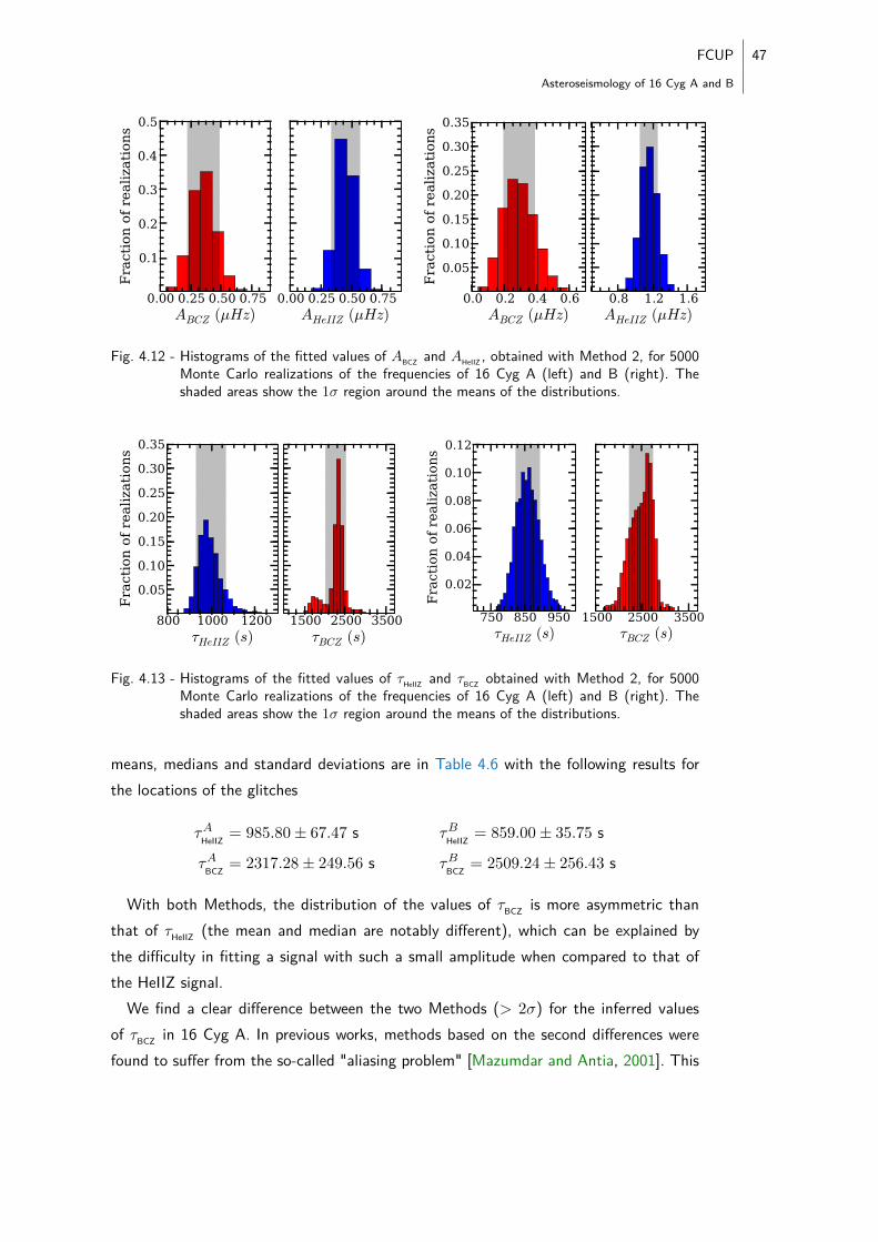
FCUP 47
Asteroseismology of 16 Cyg A and B
0.00 0.25 0.50 0.75ABCZ (µHz)
0.1
0.2
0.3
0.4
0.5F
ract
ion
of
reali
zati
on
s
0.00 0.25 0.50 0.75AHeIIZ (µHz)
0.0 0.2 0.4 0.6ABCZ (µHz)
0.05
0.10
0.15
0.20
0.25
0.30
0.35
Fra
ctio
n o
f re
ali
zati
on
s
0.8 1.2 1.6AHeIIZ (µHz)
Fig. 4.12 - Histograms of the fitted values of ABCZ and AHeIIZ , obtained with Method 2, for 5000Monte Carlo realizations of the frequencies of 16 Cyg A (left) and B (right). Theshaded areas show the 1σ region around the means of the distributions.
800 1000 1200τHeIIZ (s)
0.05
0.10
0.15
0.20
0.25
0.30
0.35
Fra
ctio
n o
f re
ali
zati
on
s
1500 2500 3500τBCZ (s)
750 850 950τHeIIZ (s)
0.02
0.04
0.06
0.08
0.10
0.12F
ract
ion
of
reali
zati
on
s
1500 2500 3500τBCZ (s)
Fig. 4.13 - Histograms of the fitted values of τHeIIZ and τBCZ obtained with Method 2, for 5000Monte Carlo realizations of the frequencies of 16 Cyg A (left) and B (right). Theshaded areas show the 1σ region around the means of the distributions.
means, medians and standard deviations are in Table 4.6 with the following results forthe locations of the glitches
τAHeIIZ = 985.80± 67.47 s τBHeIIZ = 859.00± 35.75 s
τABCZ = 2317.28± 249.56 s τBBCZ = 2509.24± 256.43 s
With both Methods, the distribution of the values of τBCZ is more asymmetric thanthat of τHeIIZ (the mean and median are notably different), which can be explained bythe difficulty in fitting a signal with such a small amplitude when compared to that ofthe HeIIZ signal.We find a clear difference between the two Methods (> 2σ) for the inferred values
of τBCZ in 16 Cyg A. In previous works, methods based on the second differences werefound to suffer from the so-called "aliasing problem" [Mazumdar and Antia, 2001]. This
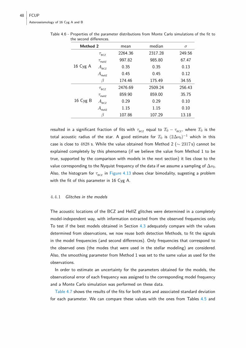
48 FCUPAsteroseismology of 16 Cyg A and B
Table 4.6 - Properties of the parameter distributions from Monte Carlo simulations of the fit tothe second differences.
Method 2 mean median σ
16 Cyg A
τBCZ 2264.36 2317.28 249.56τHeIIZ 997.82 985.80 67.47ABCZ 0.35 0.35 0.13AHeIIZ 0.45 0.45 0.12β 174.46 175.49 34.55
16 Cyg B
τBCZ 2476.69 2509.24 256.43τHeIIZ 859.90 859.00 35.75ABCZ 0.29 0.29 0.10AHeIIZ 1.15 1.15 0.10β 107.86 107.29 13.18
resulted in a significant fraction of fits with τBCZ equal to T0 − τBCZ , where T0 is thetotal acoustic radius of the star. A good estimate for T0 is (2∆ν0)−1 which in thiscase is close to 4828 s. While the value obtained from Method 2 (∼ 2317 s) cannot beexplained completely by this phenomena (if we believe the value from Method 1 to betrue, supported by the comparison with models in the next section) it lies close to thevalue corresponding to the Nyquist frequency of the data if we assume a sampling of ∆ν0.Also, the histogram for τBCZ in Figure 4.13 shows clear bimodality, sugesting a problemwith the fit of this parameter in 16 Cyg A.
4.4.1 Glitches in the models
The acoustic locations of the BCZ and HeIIZ glitches were determined in a completelymodel-independent way, with information extracted from the observed frequencies only.To test if the best models obtained in Section 4.3 adequately compare with the valuesdetermined from observations, we now reuse both detection Methods, to fit the signalsin the model frequencies (and second differences). Only frequencies that correspond tothe observed ones (the modes that were used in the stellar modeling) are considered.Also, the smoothing parameter from Method 1 was set to the same value as used for theobservations.In order to estimate an uncertainty for the parameters obtained for the models, the
observational error of each frequency was assigned to the corresponding model frequencyand a Monte Carlo simulation was performed on these data.Table 4.7 shows the results of the fits for both stars and associated standard deviation
for each parameter. We can compare these values with the ones from Tables 4.5 and
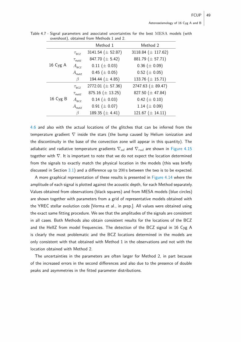
FCUP 49
Asteroseismology of 16 Cyg A and B
Table 4.7 - Signal parameters and associated uncertainties for the best MESA models (withovershoot), obtained from Methods 1 and 2.
Method 1 Method 2
16 Cyg A
τBCZ 3141.54 (± 52.87) 3118.84 (± 117.62)τHeIIZ 847.70 (± 5.42) 881.79 (± 57.71)ABCZ 0.11 (± 0.03) 0.36 (± 0.09)AHeIIZ 0.45 (± 0.05) 0.52 (± 0.05)β 194.44 (± 4.85) 133.76 (± 15.71)
16 Cyg B
τBCZ 2772.01 (± 57.36) 2747.63 (± 89.47)τHeIIZ 875.16 (± 13.25) 827.50 (± 47.84)ABCZ 0.14 (± 0.03) 0.42 (± 0.10)AHeIIZ 0.91 (± 0.07) 1.14 (± 0.09)β 189.35 (± 4.41) 121.67 (± 14.11)
4.6 and also with the actual locations of the glitches that can be inferred from thetemperature gradient ∇ inside the stars (the bump caused by Helium ionization andthe discontinuity in the base of the convection zone will appear in this quantity). Theadiabatic and radiative temperature gradients ∇ad and ∇rad are shown in Figure 4.15together with ∇. It is important to note that we do not expect the location determinedfrom the signals to exactly match the physical location in the models (this was brieflydiscussed in Section 3.1) and a difference up to 200 s between the two is to be expected.A more graphical representation of these results is presented in Figure 4.14 where the
amplitude of each signal is plotted against the acoustic depth, for each Method separately.Values obtained from observations (black squares) and from MESA models (blue circles)are shown together with parameters from a grid of representative models obtained withthe YREC stellar evolution code [Verma et al., in prep.]. All values were obtained usingthe exact same fitting procedure. We see that the amplitudes of the signals are consistentin all cases. Both Methods also obtain consistent results for the locations of the BCZand the HeIIZ from model frequencies. The detection of the BCZ signal in 16 Cyg Ais clearly the most problematic and the BCZ locations determined in the models areonly consistent with that obtained with Method 1 in the observations and not with thelocation obtained with Method 2.The uncertainties in the parameters are often larger for Method 2, in part because
of the increased errors in the second differences and also due to the presence of doublepeaks and asymmetries in the fitted parameter distributions.
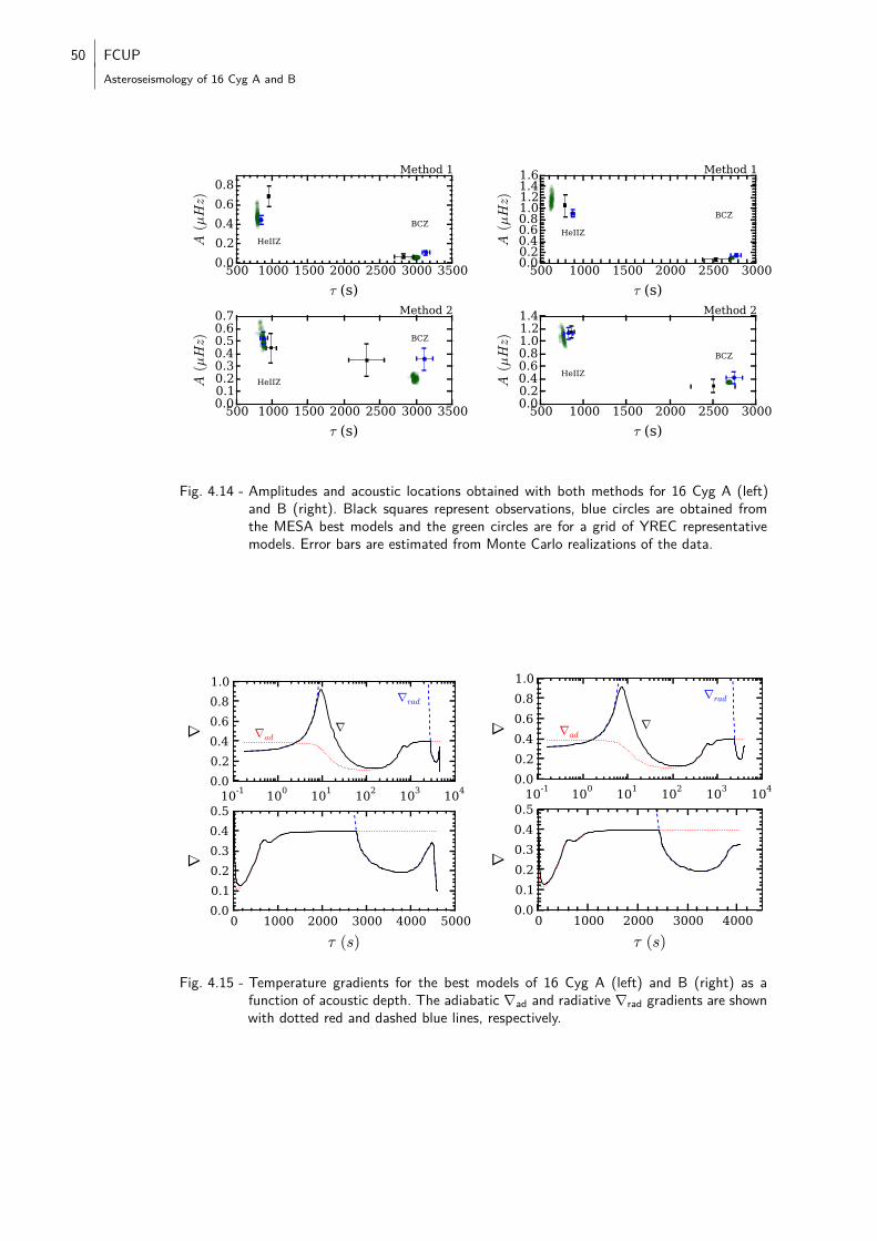
50 FCUPAsteroseismology of 16 Cyg A and B
500 1000 1500 2000 2500 3000 3500
τ (s)
0.0
0.2
0.4
0.6
0.8A
(µHz)
BCZ
HeIIZ
Method 1
500 1000 1500 2000 2500 3000 3500
τ (s)
0.00.10.20.30.40.50.60.7
A(µHz) BCZ
HeIIZ
Method 2
500 1000 1500 2000 2500 3000
τ (s)
0.00.20.40.60.81.01.21.41.6
A(µHz)
BCZ
HeIIZ
Method 1
500 1000 1500 2000 2500 3000
τ (s)
0.00.20.40.60.81.01.21.4
A(µHz)
BCZ
HeIIZ
Method 2
Fig. 4.14 - Amplitudes and acoustic locations obtained with both methods for 16 Cyg A (left)and B (right). Black squares represent observations, blue circles are obtained fromthe MESA best models and the green circles are for a grid of YREC representativemodels. Error bars are estimated from Monte Carlo realizations of the data.
10-1 100 101 102 103 1040.00.20.40.60.81.0
∇ ∇ad
∇rad
∇
0 1000 2000 3000 4000 5000τ (s)
0.00.10.20.30.40.5
∇
10-1 100 101 102 103 1040.00.20.40.60.81.0
∇ ∇ad
∇rad
∇
0 1000 2000 3000 4000τ (s)
0.00.10.20.30.40.5
∇
Fig. 4.15 - Temperature gradients for the best models of 16 Cyg A (left) and B (right) as afunction of acoustic depth. The adiabatic ∇ad and radiative ∇rad gradients are shownwith dotted red and dashed blue lines, respectively.
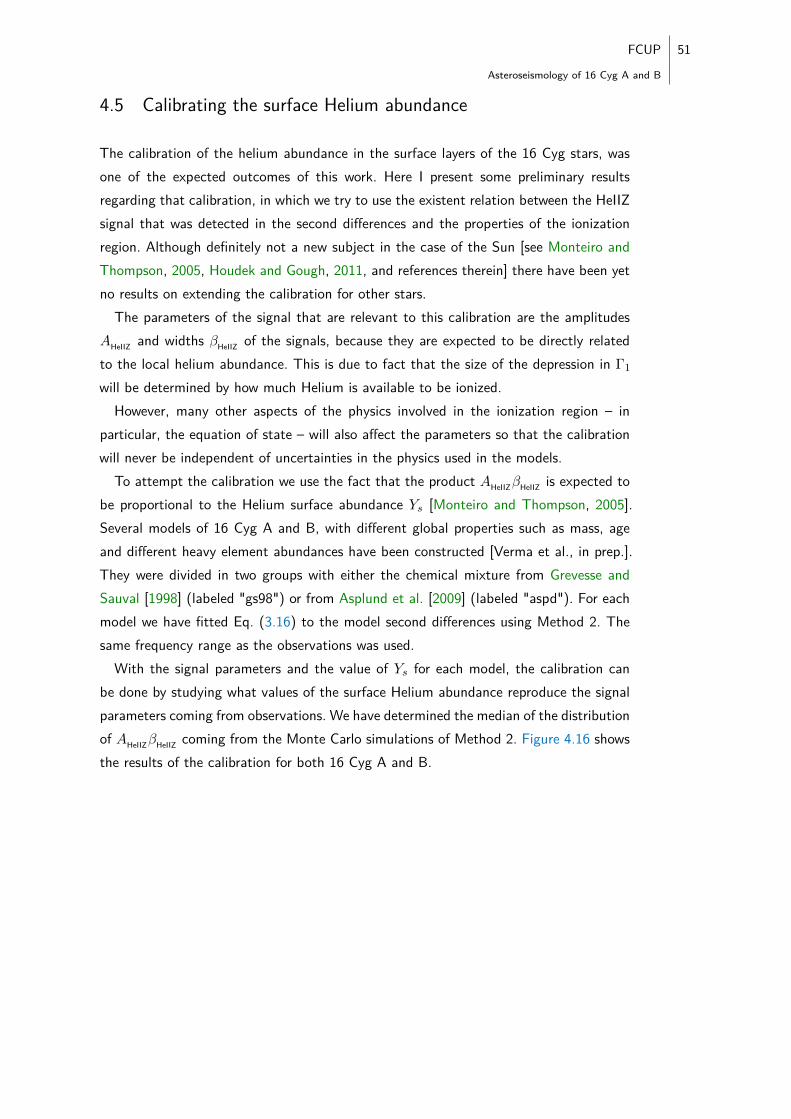
FCUP 51
Asteroseismology of 16 Cyg A and B
4.5 Calibrating the surface Helium abundance
The calibration of the helium abundance in the surface layers of the 16 Cyg stars, wasone of the expected outcomes of this work. Here I present some preliminary resultsregarding that calibration, in which we try to use the existent relation between the HeIIZsignal that was detected in the second differences and the properties of the ionizationregion. Although definitely not a new subject in the case of the Sun [see Monteiro andThompson, 2005, Houdek and Gough, 2011, and references therein] there have been yetno results on extending the calibration for other stars.The parameters of the signal that are relevant to this calibration are the amplitudes
AHeIIZ and widths βHeIIZ of the signals, because they are expected to be directly relatedto the local helium abundance. This is due to fact that the size of the depression in Γ1
will be determined by how much Helium is available to be ionized.However, many other aspects of the physics involved in the ionization region – in
particular, the equation of state – will also affect the parameters so that the calibrationwill never be independent of uncertainties in the physics used in the models.
To attempt the calibration we use the fact that the product AHeIIZβHeIIZ is expected tobe proportional to the Helium surface abundance Ys [Monteiro and Thompson, 2005].Several models of 16 Cyg A and B, with different global properties such as mass, ageand different heavy element abundances have been constructed [Verma et al., in prep.].They were divided in two groups with either the chemical mixture from Grevesse andSauval [1998] (labeled "gs98") or from Asplund et al. [2009] (labeled "aspd"). For eachmodel we have fitted Eq. (3.16) to the model second differences using Method 2. Thesame frequency range as the observations was used.With the signal parameters and the value of Ys for each model, the calibration can
be done by studying what values of the surface Helium abundance reproduce the signalparameters coming from observations. We have determined the median of the distributionof AHeIIZβHeIIZ coming from the Monte Carlo simulations of Method 2. Figure 4.16 showsthe results of the calibration for both 16 Cyg A and B.
52 FCUPAsteroseismology of 16 Cyg A and B
0.18 0.20 0.22 0.24 0.26 0.28 0.30Ys
50
60
70
80
90
100
(Aβ) H
eIIZ
obs
gs98aspd
0.18 0.20 0.22 0.24 0.26 0.28 0.30Ys
110
115
120
125
130
135
140
145
(Aβ) H
eIIZ
obs
gs98aspd
Fig. 4.16 - Calibration of the Helium surface abundance for 16 Cyg A (left) and B (right). Thesymbols show the quantity AHeIIZβHeIIZ obtained from the frequencies of models withdifferent chemical mixtures, as function of model surface Helium abundance. Theobservational value from Monte Carlo simulations is also shown (labeled "obs").
A value of Ys in the range 0.24 − 0.26 is suggested by the observations, when con-sidering models with these particular characteristics, although no extensive study of theuncertainties associated with the calibration has been carried out yet.
5Conclusion
An asteroseismic study of the two stars 16 Cyg A and B was conducted, based onoscillation frequencies obtained from nine months of Kepler photometric time seriesdata. This set of frequencies is of outstanding quality, with mean uncertainties under1µHz and a total of 60 or more modes detected for each star. Several diagnostics thatuse combinations or intrinsic properties of the frequencies were studied in an attempt toextract useful information about the stellar interiors.The ratios of small to large separations were added as a seismic constraint in the
forward modeling approach with MESA. In principle, we could obtain models that betterrepresent the interior regions of the stars because the ratios are virtually independent ofthe structure of the outer layers and also do not rely on the empirical surface correction,as do the frequencies. However, since the frequencies were also included in the χ2, thisadvantage might be mitigated by an unknown bias caused by the correction which willstill be present.Also, the ratios (especially those of 16 Cyg A) show higher variability in the high
frequency regime which can be an intrinsic behavior that is not being reproduced bythe models, or an effect of the increased errors. The points with smaller frequency willcontribute more to the component of the χ2 that includes the ratios, because of theirsmaller uncertainties. It seems though that during the search for the best model, andprobably because there is no model that matches closely the observed behavior, thehigher frequency points are being "averaged out" (this is especially noticeable in theleft panel of Figure 4.7). This might be introducing an unknown bias in the results.Nevertheless, the justification to include every available observed frequency, regardlessof the associated uncertainty is still valid.We have obtained two best models for each star (Table 4.4), either considering an
overshoot parameter fov as a free parameter or setting it to zero. Two different andindependent searches were performed to find the best fitting models, so that the effectof including overshoot mixing cannot be inferred from comparing the two resulting bestmodels [on this subject see, e. g., Marques et al., 2004, 2005]. We find that the addeddegree of freedom from letting fov vary resulted in models in closer agreement with thespectroscopic constraints and that also agree in properties that should be common toboth stars, like the stellar ages.
53
54 FCUPAsteroseismology of 16 Cyg A and B
Since we did not use the same set of frequencies as Metcalfe et al. [2012] and alsodid not consider the same spectroscopic constraints, some differences in the best modelparameters are to be expected (recent works show that such differences can even originatefrom a simple change in the fitting method [Gruberbauer et al., 2013]). It is neverthelessreassuring that the best models obtained from MESA are not completely discrepantfrom those obtained with other methods.The abrupt changes in the stratification of a star, connected with the regions of ion-
ization of helium and the base of the convection zone, were also studied in depth. Theseacoustic glitches produce a characteristic oscillatory signal in the oscillation frequenciesthat can be detected and characterized. In that way, we were able to extract informationabout the interior regions of the star where the signals originated from.The development and improvement of two different methods to characterize the above
mentioned signals are a cornerstone of this work. They fit to the frequencies or tothe second differences an appropriate functional form for the signal and the resultingparameters describe, among other properties, an estimate of the acoustic locations ofthe glitches.The amplitude of the signals in the second differences is enhanced relative to a smooth
component that is present in both frequencies and second differences. This smoothcomponent needs to be removed before fitting the signals and the two methods discussedhere achieve this in different ways. Method 1 does not assume a functional form forthe smooth function but it does depend on a parametric fit to remove it, introducinga parameter λ that is difficult to constrain. Method 2 assumes a simpler constant orpolynomial function. We have determined that the fitted amplitudes (in representativemodels) do not show the magnification expected from theoretical calculations. This canbe because the two methods do not remove exactly the same smooth function.As a result, there is no clear advantage in using the second differences to detect the
HeIIZ signal. For the BCZ signal there is an amplitude magnification but, as we see inFigure 4.14, the increased uncertainties on the second differences propagate to the fitparameters adding to the uncertainties in the latter.Overall, both methods end up giving consistent results in most aspects, although
Method 1 seems less prone to contamination in the smaller amplitude signal from thebase of the convection zone and compares favorably with results from the MESA bestmodels. Our conclusion is that both Methods benefit from the improvements studiedand applied here and can provide interesting results for other solar-type stars.With this methodology we have determined the acoustic depth of the base of the
convection zone and the second helium ionization region for both stars. Another charac-teristic of the signal, that relates directly with the Helium abundance in the surface, was
FCUP 55
Asteroseismology of 16 Cyg A and B
used to attempt a calibration of this quantity. We have obtained a range of values forYs which is favored by the observations. Although still work in progress, this calibrationcan provide a more direct way of determining the helium abundance of a star.
The outstanding data available from the Kepler mission is only now beginning to be fullyexploited†. At the same time, the best methods to perform a complete and thoroughanalysis of these data, are still being devised. The goals of this work were to study andimprove currently used diagnostics, in an attempt to learn more about the interiors oftwo particular stars. To the author’s knowledge, it was the first time that MESA wasused to perform asteroseismic model fitting (apart from the proof-of-concept example inPaxton et al. [2013]). We went beyond the more traditional approaches and explored theuse of the frequency ratios as more precise proxies of the deep interiors of stars. In thefuture, we expect this approach to be improved upon and stellar models to come evencloser to real stars. Additional work is still needed in developing methods that cancel thebiases resulting from the deficient modelling of the near-surface layers, like the surfacecorrections applied to the frequencies.On the study of acoustic glitches, we focused on two methods to extract and charac-
terize the oscillatory signals present in the frequencies. A model independent measure ofthe acoustic locations of the base of the convection zone and of the Helium ionizationregion can be achieved with the methods. Preliminary results show that a calibration ofthe Helium surface abundance is also possible. The two components of the 16 Cyg binarywere studied in depth with these methods. In the future, they should also be applied toother stars to, again, extract information about the stellar interiors. To facilitate reuseand reproducibility, the implementations of both methods will be made freely availableonline as open-source projects‡.To conclude, I believe the work presented here is important in the broader context of
asteroseismology, in particular, of solar-type stars. But, as any scientific endeavor, it isfar from complete and the question remains: how much more can we learn about stars?
†Despite the recent news that it might prove impossible to continue doing precision asteroseismologywith Kepler, a wealth of data is still awaiting analysis
‡See www.astro.up.pt/~jfaria/msc-thesis

Bibliography
C. Aerts, J. Christensen-Dalsgaard, and D. W. Kurtz. Asteroseismology. Astronomy andAstrophysics Library. Springer, 1st edition, 2010. URL http://amazon.com/o/ASIN/
1402051786/. (Cited on pages 7, 9, 11, and 12.)
C. Angulo, M. Arnould, M. Rayet, P. Descouvemont, D. Baye, C. Leclercq-Willain,A. Coc, S. Barhoumi, P. Aguer, C. Rolfs, R. Kunz, J. W. Hammer, A. Mayer, T. Pa-radellis, S. Kossionides, C. Chronidou, K. Spyrou, S. degl’Innocenti, G. Fiorentini,B. Ricci, S. Zavatarelli, C. Providencia, H. Wolters, J. Soares, C. Grama, J. Rahighi,A. Shotter, and M. Lamehi Rachti. A compilation of charged-particle inducedthermonuclear reaction rates. Nuclear Physics A, 656:3–183, August 1999. doi:10.1016/S0375-9474(99)00030-5. (Cited on page 38.)
T. Appourchaux, W. J. Chaplin, R. A. García, M. Gruberbauer, G. A. Verner, H. M. Antia,O. Benomar, T. L. Campante, G. R. Davies, S. Deheuvels, R. Handberg, S. Hekker,R. Howe, C. Régulo, D. Salabert, T. R. Bedding, T. R. White, J. Ballot, S. Mathur,V. Silva Aguirre, Y. P. Elsworth, S. Basu, R. L. Gilliland, J. Christensen-Dalsgaard,H. Kjeldsen, K. Uddin, M. C. Stumpe, and T. Barclay. Oscillation mode frequenciesof 61 main-sequence and subgiant stars observed by Kepler. Astronomy & Astrophysics,543:A54, July 2012. doi: 10.1051/0004-6361/201218948. (Cited on page 35.)
M. Asplund, N. Grevesse, A. J. Sauval, and P. Scott. The Chemical Composition of theSun. Annual Review of Astronomy and Astrophysics, 47:481–522, September 2009.doi: 10.1146/annurev.astro.46.060407.145222. (Cited on page 51.)
A. Baglin, M. Auvergne, P. Barge, E. Michel, C. Catala, M. Deleuil, and W. Weiss. TheCoRoT mission and its scientific objectives. In C. Dumitrache, N. A. Popescu, M. D.Suran, and V. Mioc, editors, Fifty Years of Romanian Astrophysics, volume 895 ofAmerican Institute of Physics Conference Series, pages 201–209, March 2007. doi:10.1063/1.2720423. (Cited on page 3.)
I. M. Brandão, G. Doğan, J. Christensen-Dalsgaard, M. S. Cunha, T. R. Bedding, T. S.Metcalfe, H. Kjeldsen, H. Bruntt, and T. Arentoft. Asteroseismic modelling of thesolar-type subgiant star β Hydri. Astronomy & Astrophysics, 527:A37, March 2011.doi: 10.1051/0004-6361/201015370. (Cited on page 38.)
57
58 FCUPAsteroseismology of 16 Cyg A and B
M. Brodsky and S. V. Vorontsov. Asymptotic theory of intermediate- and high-degreesolar acoustic oscillations. The Astrophysical Journal, 409:455–464, May 1993. doi:10.1086/172678. (Cited on page 17.)
A.-M. Broomhall, W. J. Chaplin, G. R. Davies, Y. Elsworth, S. T. Fletcher, S. J. Hale,B. Miller, and R. New. Definitive Sun-as-a-star p-mode frequencies: 23 years of BiSONobservations. Monthly Notices of the Royal Astronomical Society, 396:L100–L104,June 2009. doi: 10.1111/j.1745-3933.2009.00672.x. (Cited on page 27.)
C. Catala. Asteroseismology. Online, 2009. URL http://www.lesia.obspm.fr/perso/
claude-catala/plato_web_files/asteroseismology.html. (Cited on page 11.)
W. J. Chaplin, Y. Elsworth, G. R. Isaak, K. I. Marchenkov, B. A. Miller, R. New, B. Pinter,and T. Appourchaux. Peak finding at low signal-to-noise ratio: low-l solar acousticeigenmodes at n<= 9 from the analysis of BiSON data. Monthly Notices of the RoyalAstronomical Society, 336:979–991, November 2002. doi: 10.1046/j.1365-8711.2002.05834.x. (Cited on page 12.)
W. J. Chaplin, H. Kjeldsen, J. Christensen-Dalsgaard, S. Basu, A. Miglio, T. Appour-chaux, T. R. Bedding, Y. Elsworth, R. A. García, R. L. Gilliland, L. Girardi, G. Houdek,C. Karoff, S. D. Kawaler, T. S. Metcalfe, J. Molenda-Żakowicz, M. J. P. F. G. Monteiro,M. J. Thompson, G. A. Verner, J. Ballot, A. Bonanno, I. M. Brandão, A.-M. Broomhall,H. Bruntt, T. L. Campante, E. Corsaro, O. L. Creevey, G. Doğan, L. Esch, N. Gai,P. Gaulme, S. J. Hale, R. Handberg, S. Hekker, D. Huber, A. Jiménez, S. Mathur,A. Mazumdar, B. Mosser, R. New, M. H. Pinsonneault, D. Pricopi, P.-O. Quirion,C. Régulo, D. Salabert, A. M. Serenelli, V. Silva Aguirre, S. G. Sousa, D. Stello, I. R.Stevens, M. D. Suran, K. Uytterhoeven, T. R. White, W. J. Borucki, T. M. Brown,J. M. Jenkins, K. Kinemuchi, J. Van Cleve, and T. C. Klaus. Ensemble Asteroseis-mology of Solar-Type Stars with the NASA Kepler Mission. Science, 332:213–, April2011. doi: 10.1126/science.1201827. (Cited on page 3.)
P. Charbonneau. Genetic Algorithms in Astronomy and Astrophysics. The Astrophysi-cal Journal Supplement, 101:309, December 1995. doi: 10.1086/192242. (Cited onpage 26.)
P. Charbonneau. Release Notes for PIKAIA 1.2. NCAR Technical Note 451, Boulder:National Center for Atmospheric Research, 2002. (Cited on page 27.)
J. Christensen-Dalsgaard. Some aspects of the theory of solar oscillations. Geo-physical and Astrophysical Fluid Dynamics, 62:123–152, 1991. doi: 10.1080/
03091929108229129. (Cited on page 8.)
FCUP 59
Asteroseismology of 16 Cyg A and B
J. Christensen-Dalsgaard. Helioseismology. Reviews of Modern Physics, 74:1073–1129,November 2002. doi: 10.1103/RevModPhys.74.1073. (Cited on page 2.)
J. Christensen-Dalsgaard. ADIPLS - the Aarhus adiabatic oscillation package.Astrophysics and Space Science, 316:113–120, August 2008. doi: 10.1007/
s10509-007-9689-z. (Cited on page 4.)
W. D. Cochran, A. P. Hatzes, R. P. Butler, and G. W. Marcy. The Discovery of aPlanetary Companion to 16 Cygni B. The Astrophysical Journal, 483:457, July 1997.doi: 10.1086/304245. (Cited on page 33.)
T. G. Cowling. The non-radial oscillations of polytropic stars. Monthly Notices of theRoyal Astronomical Society, 101:367, 1941. (Cited on page 8.)
Arthur N. Cox, editor. Allen’s Astrophysical Quantities. Springer, 4th edition, 4 2001.ISBN 9780387951898. URL http://amazon.com/o/ASIN/038795189X/. (Cited onpage 34.)
John P. Cox and R. Thomas Giuli. Principles of Stellar Structure. Gordon and Breach,Science Publishers, 1968. (Cited on page 38.)
M. S. Cunha, C. Aerts, J. Christensen-Dalsgaard, A. Baglin, L. Bigot, T. M. Brown,C. Catala, O. L. Creevey, A. Domiciano de Souza, P. Eggenberger, P. J. V. Garcia,F. Grundahl, P. Kervella, D. W. Kurtz, P. Mathias, A. Miglio, M. J. P. F. G. Monteiro,G. Perrin, F. P. Pijpers, D. Pourbaix, A. Quirrenbach, K. Rousselet-Perraut, T. C. Teix-eira, F. Thévenin, and M. J. Thompson. Asteroseismology and interferometry. As-tronomy & Astrophysics Review, 14:217–360, 2007. doi: 10.1007/s00159-007-0007-0.(Cited on pages 2 and 13.)
F.-L. Deubner and D. Gough. Helioseismology: Oscillations as a Daignostic of the SolarInterior. Annual Review of Astronomy and Astrophysics, 22:593–619, 1984. doi:10.1146/annurev.aa.22.090184.003113. (Cited on page 8.)
S. Dodelson and M. D. Schneider. Simulation Covariance Error. ArXiv e-prints, April2013. arXiv:1304.2593. (Cited on page 26.)
J. W. Ferguson, D. R. Alexander, F. Allard, T. Barman, J. G. Bodnarik, P. H. Hauschildt,A. Heffner-Wong, and A. Tamanai. Low-Temperature Opacities. The AstrophysicalJournal, 623:585–596, April 2005. doi: 10.1086/428642. (Cited on page 38.)
R. A. García, S. Hekker, D. Stello, J. Gutiérrez-Soto, R. Handberg, D. Huber, C. Karoff,K. Uytterhoeven, T. Appourchaux, W. J. Chaplin, Y. Elsworth, S. Mathur, J. Ballot,
60 FCUPAsteroseismology of 16 Cyg A and B
J. Christensen-Dalsgaard, R. L. Gilliland, G. Houdek, J. M. Jenkins, H. Kjeldsen, S. Mc-Cauliff, T. Metcalfe, C. K. Middour, J. Molenda-Zakowicz, M. J. P. F. G. Monteiro,J. C. Smith, and M. J. Thompson. Preparation of Kepler light curves for asteroseismicanalyses. Monthly Notices of the Royal Astronomical Society, 414:L6–L10, June 2011.doi: 10.1111/j.1745-3933.2011.01042.x. (Cited on page 35.)
R. L. Gilliland, T. M. Brown, J. Christensen-Dalsgaard, H. Kjeldsen, C. Aerts, T. Ap-pourchaux, S. Basu, T. R. Bedding, W. J. Chaplin, M. S. Cunha, P. De Cat, J. DeRidder, J. A. Guzik, G. Handler, S. Kawaler, L. Kiss, K. Kolenberg, D. W. Kurtz, T. S.Metcalfe, M. J. P. F. G. Monteiro, R. Szabó, T. Arentoft, L. Balona, J. Debosscher,Y. P. Elsworth, P.-O. Quirion, D. Stello, J. C. Suárez, W. J. Borucki, J. M. Jenkins,D. Koch, Y. Kondo, D. W. Latham, J. F. Rowe, and J. H. Steffen. Kepler Astero-seismology Program: Introduction and First Results. Publications of the AstronomicalSociety of the Pacific, 122:131–143, February 2010. doi: 10.1086/650399. (Cited onpage 3.)
D. Gough. Comments on helioseismic inference. In Y. Osaki and H. Shibahashi, editors,Progress of Seismology of the Sun and Stars, volume 367 of Lecture Notes in Physics,Berlin Springer Verlag, page 281, 1990. doi: 10.1007/3-540-53091-6_93. (Cited onpage 3.)
D. Gough and J. Toomre. Seismic observations of the solar interior. Annual Review ofAstronomy and Astrophysics, 29:627–685, 1991. doi: 10.1146/annurev.aa.29.090191.003211. (Cited on page 2.)
D. O. Gough. Linear adiabatic stellar pulsation. In J.-P. Zahn and J. Zinn-Justin, editors,Astrophysical Fluid Dynamics - Les Houches 1987, pages 399–560, 1993. (Cited onpage 9.)
D. O. Gough. An elementary introduction to the JWKB approximation. AstronomischeNachrichten, 328:273, March 2007. doi: 10.1002/asna.200610730. (Cited on page 9.)
G. Grec, E. Fossat, and M. A. Pomerantz. Full-disk observations of solar oscillationsfrom the geographic South Pole - Latest results. Solar Physics, 82:55–66, January1983. doi: 10.1007/BF00145545. (Cited on page 10.)
N. Grevesse and A. J. Sauval. Standard Solar Composition. Space Science Reviews, 85:161–174, May 1998. doi: 10.1023/A:1005161325181. (Cited on page 51.)
M. Gruberbauer, D. B. Guenther, K. MacLeod, and T. Kallinger. Bayesian Asteroseis-mology of 23 Solar-Like Kepler Targets. ArXiv 1307.4218G, July 2013. (Cited onpage 54.)
FCUP 61
Asteroseismology of 16 Cyg A and B
H. M. Hauser and G. W. Marcy. The Orbit of 16 Cygni AB. Publications of theAstronomical Society of the Pacific, 111:321–334, March 1999. doi: 10.1086/316328.(Cited on page 34.)
F. Herwig. The evolution of AGB stars with convective overshoot. Astronomy & Astro-physics, 360:952–968, August 2000. (Cited on page 39.)
G. Houdek. Convection and oscillations. Astronomische Nachrichten, 331:998–1003,December 2010. doi: 10.1002/asna.201011445. (Cited on page 3.)
G. Houdek and D. O. Gough. An asteroseismic signature of helium ionization. MonthlyNotices of the Royal Astronomical Society, 375:861–880, March 2007. doi: 10.1111/j.1365-2966.2006.11325.x. (Cited on pages 14, 20, 22, 23, 28, and 30.)
G. Houdek and D. O. Gough. On the seismic age and heavy-element abundance of theSun. Monthly Notices of the Royal Astronomical Society, 418:1217–1230, December2011. doi: 10.1111/j.1365-2966.2011.19572.x. (Cited on page 51.)
D. Huber, D. Stello, T. R. Bedding, W. J. Chaplin, T. Arentoft, P.-O. Quirion, andH. Kjeldsen. Automated extraction of oscillation parameters for Kepler observationsof solar-type stars. Communications in Asteroseismology, 160:74, October 2009. (Citedon page 35.)
C. A. Iglesias and F. J. Rogers. Radiative opacities for carbon- and oxygen-rich mixtures.The Astrophysical Journal, 412:752–760, August 1993. doi: 10.1086/172958. (Citedon page 38.)
C. A. Iglesias and F. J. Rogers. Updated Opal Opacities. The Astrophysical Journal,464:943, June 1996. doi: 10.1086/177381. (Cited on page 38.)
H. Kjeldsen, T. R. Bedding, and J. Christensen-Dalsgaard. Correcting Stellar OscillationFrequencies for Near-Surface Effects. The Astrophysical Journal Letters, 683:L175–L178, August 2008. doi: 10.1086/591667. (Cited on pages 3, 37, and 38.)
K. I. Marchenkov and S. V. Vorontsov. Seismic probing of outer regions of the sun. SovietAstronomy Letters, 133:149–154, May 1991. doi: 10.1007/BF00149836. (Cited onpage 19.)
J. P. Marques, J. Fernandes, and M. J. P. F. G. Monteiro. The role of the time step andovershooting in the modelling of PMS evolution: The case of EK Cephei. Astronomy& Astrophysics, 422:239–245, July 2004. doi: 10.1051/0004-6361:20035693. (Citedon page 53.)
62 FCUPAsteroseismology of 16 Cyg A and B
J. P. Marques, M. J. P. F. G. Monteiro, and J. Fernandes. Effects of convective over-shooting in the PMS evolution of intermediate mass stars. In F. Favata, G. A. J.Hussain, and B. Battrick, editors, 13th Cambridge Workshop on Cool Stars, StellarSystems and the Sun, volume 560 of ESA Special Publication, page 795, March 2005.(Cited on page 53.)
J. P. Marques, M. J. P. F. G. Monteiro, and J. M. Fernandes. Grids of stellar evolutionmodels for asteroseismology ( cesam + posc). Astrophysics and Space Science, 316:173–178, August 2008. doi: 10.1007/s10509-008-9786-7. (Cited on pages 33 and 34.)
A. Mazumdar and H. M. Antia. Seismic study of stellar convective cores. Astronomy &Astrophysics, 377:192–205, October 2001. doi: 10.1051/0004-6361:20011072. (Citedon page 47.)
A. Mazumdar, M. J. P. F. G. Monteiro, J. Ballot, H. M. Antia, S. Basu, G. Houdek,S. Mathur, M. S. Cunha, V. Silva Aguirre, R. A. García, D. Salabert, G. A. Verner,J. Christensen-Dalsgaard, T. S. Metcalfe, and W. J. Chaplin. Acoustic glitches insolar-type stars from Kepler. Astronomische Nachrichten, 333:1040–1043, December2012. doi: 10.1002/asna.201211825. (Cited on pages 4, 22, 23, and 24.)
T. S. Metcalfe, W. J. Chaplin, T. Appourchaux, R. A. García, S. Basu, I. Brandão, O. L.Creevey, S. Deheuvels, G. Dogan, P. Eggenberger, C. Karoff, A. Miglio, D. Stello,M. Yıldız, Z. Çelik, H. M. Antia, O. Benomar, R. Howe, C. Régulo, D. Salabert,T. Stahn, T. R. Bedding, G. R. Davies, Y. Elsworth, L. Gizon, S. Hekker, S. Mathur,B. Mosser, S. T. Bryson, M. D. Still, J. Christensen-Dalsgaard, R. L. Gilliland, S. D.Kawaler, H. Kjeldsen, K. A. Ibrahim, T. C. Klaus, and J. Li. Asteroseismology of theSolar Analogs 16 Cyg A and B from Kepler Observations. The Astrophysical JournalLetters, 748:L10, March 2012. doi: 10.1088/2041-8205/748/1/L10. (Cited on pages 3,35, 39, 41, 42, and 54.)
M. J. P. F. G. Monteiro and M. J. Thompson. Seismic analysis of the second ioniza-tion region of helium in the Sun - I. Sensitivity study and methodology. MonthlyNotices of the Royal Astronomical Society, 361:1187–1196, August 2005. doi:10.1111/j.1365-2966.2005.09246.x. (Cited on pages 4, 17, 20, 21, 23, 27, and 51.)
M. J. P. F. G. Monteiro, J. Christensen-Dalsgaard, and M. J. Thompson. Seismic studyof overshoot at the base of the solar convective envelope. Astronomy & Astrophysics,283:247–262, March 1994. (Cited on pages 17, 18, 20, 21, 23, 24, and 27.)
M. J. P. F. G. Monteiro, J. Christensen-Dalsgaard, and M. J. Thompson. Seismic studyof stellar convective regions: the base of the convective envelope in low-mass stars.
FCUP 63
Asteroseismology of 16 Cyg A and B
Monthly Notices of the Royal Astronomical Society, 316:165–172, July 2000. doi:10.1046/j.1365-8711.2000.03471.x. (Cited on page 23.)
J. A. Nelder and R. Mead. A Simplex Method for Function Minimization. The ComputerJournal, 7(4):308–313, 1965. doi: 10.1093/comjnl/7.4.308. (Cited on page 37.)
H. Otí Floranes, J. Christensen-Dalsgaard, and M. J. Thompson. The use of frequency-separation ratios for asteroseismology. Monthly Notices of the Royal AstronomicalSociety, 356:671–679, January 2005. doi: 10.1111/j.1365-2966.2004.08487.x. (Citedon page 11.)
J. Patience, R. J. White, A. M. Ghez, C. McCabe, I. S. McLean, J. E. Larkin, L. Prato,S. S. Kim, J. P. Lloyd, M. C. Liu, J. R. Graham, B. A. Macintosh, D. T. Gavel, C. E.Max, B. J. Bauman, S. S. Olivier, P. Wizinowich, and D. S. Acton. Stellar Companionsto Stars with Planets. The Astrophysical Journal, 581:654–665, December 2002. doi:10.1086/342982. (Cited on page 33.)
B. Paxton, L. Bildsten, A. Dotter, F. Herwig, P. Lesaffre, and F. Timmes. Modules forExperiments in Stellar Astrophysics (MESA). The Astrophysical Journal Supplement,192:3, January 2011. doi: 10.1088/0067-0049/192/1/3. (Cited on pages 4 and 38.)
B. Paxton, M. Cantiello, P. Arras, L. Bildsten, E. F. Brown, A. Dotter, C. Mankovich,M. H. Montgomery, D. Stello, F. X. Timmes, and R. Townsend. Modules for Ex-periments in Stellar Astrophysics (MESA): Giant Planets, Oscillations, Rotation, andMassive Stars. ArXiv e-prints, January 2013. (Cited on pages 4, 37, and 55.)
D. Raghavan, T. J. Henry, B. D. Mason, J. P. Subasavage, W.-C. Jao, T. D. Beaulieu,and N. C. Hambly. Two Suns in The Sky: Stellar Multiplicity in Exoplanet Systems.The Astrophysical Journal, 646:523–542, July 2006. doi: 10.1086/504823. (Cited onpage 33.)
I. Ramírez, J. Meléndez, and M. Asplund. Accurate abundance patterns of solar twins andanalogs. Does the anomalous solar chemical composition come from planet formation?Astronomy & Astrophysics, 508:L17–L20, December 2009. doi: 10.1051/0004-6361/200913038. (Cited on pages 33, 34, and 41.)
F. J. Rogers and A. Nayfonov. Updated and Expanded OPAL Equation-of-State Tables:Implications for Helioseismology. The Astrophysical Journal, 576:1064–1074, Septem-ber 2002. doi: 10.1086/341894. (Cited on page 38.)
I. W. Roxburgh and S. V. Vorontsov. Seismology of the Solar Envelope - the Base ofthe Convective Zone as Seen in the Phase Shift of Acoustic Waves. Monthly Noticesof the Royal Astronomical Society, 268:880, June 1994. (Cited on page 19.)
64 FCUPAsteroseismology of 16 Cyg A and B
I. W. Roxburgh and S. V. Vorontsov. The ratio of small to large separations of acousticoscillations as a diagnostic of the interior of solar-like stars. Astronomy & Astrophysics,411:215–220, November 2003. doi: 10.1051/0004-6361:20031318. (Cited on pages 11and 12.)
S. C. Schuler, K. Cunha, V. V. Smith, L. Ghezzi, J. R. King, C. P. Deliyannis, and A. M.Boesgaard. Detailed Abundances of the Solar Twins 16 Cygni A and B: ConstrainingPlanet Formation Models. The Astrophysical Journal Letters, 737:L32, August 2011.doi: 10.1088/2041-8205/737/2/L32. (Cited on page 33.)
V. Silva Aguirre, S. Basu, I. M. Brandão, J. Christensen-Dalsgaard, S. Deheuvels,G. Doğan, T. S. Metcalfe, A. M. Serenelli, J. Ballot, W. J. Chaplin, M. S. Cunha,A. Weiss, T. Appourchaux, L. Casagrande, S. Cassisi, O. L. Creevey, R. A. García,Y. Lebreton, A. Noels, S. G. Sousa, D. Stello, T. R. White, S. D. Kawaler, andH. Kjeldsen. Stellar Ages and Convective Cores in Field Main-sequence Stars: FirstAsteroseismic Application to Two Kepler Targets. The Astrophysical Journal, 769:141,June 2013. doi: 10.1088/0004-637X/769/2/141. (Cited on page 38.)
James O. Street, Raymond J. Carroll, and David Ruppert. A Note on Computing Ro-bust Regression Estimates Via Iteratively Reweighted Least Squares. The AmericanStatistician, 42(2):pp. 152–154, 1988. ISSN 00031305. URL http://www.jstor.
org/stable/2684491. (Cited on page 26.)
M. Tassoul. Asymptotic approximations for stellar nonradial pulsations. The Astrophys-ical Journal Supplement, 43:469–490, August 1980. doi: 10.1086/190678. (Cited onpage 9.)
M. Tassoul. Second-order asymptotic approximations for stellar nonradial acoustic modes.The Astrophysical Journal, 358:313–327, July 1990. doi: 10.1086/168988. (Cited onpage 9.)
A. A. Thoul, J. N. Bahcall, and A. Loeb. Element diffusion in the solar interior. TheAstrophysical Journal, 421:828–842, February 1994. doi: 10.1086/173695. (Cited onpage 38.)
N. H. Turner, T. A. ten Brummelaar, H. A. McAlister, B. D. Mason, W. I. Hartkopf, andL. C. Roberts, Jr. Search for Faint Companions to Nearby Solar-like Stars using theAdaptive Optics System at Mount Wilson Observatory. The Astrophysical Journal,121:3254–3258, June 2001. doi: 10.1086/321075. (Cited on page 33.)
FCUP 65
Asteroseismology of 16 Cyg A and B
Wasaburo Unno, Yoji Osaki, Hiroyasu Ando, H. Saio, and H. Shibahashi. NonradialOscillations of Stars. University of Tokyo Press, 2nd edition, 1989. URL http://
adsabs.harvard.edu/abs/1989nos..book.....U. (Cited on page 7.)
F. van Leeuwen. Validation of the new Hipparcos reduction. Astronomy & Astrophysics,474:653–664, November 2007. doi: 10.1051/0004-6361:20078357. (Cited on page 34.)
S. V. Vorontsov and V. N. Zharkov. Helioseismology - Theory and Interpretation ofExperimental Data. Astrophysics and Space Physics Reviews, 7:1, 1989. (Cited onpage 19.)
T. R. White, D. Huber, V. Maestro, T. R. Bedding, M. J. Ireland, F. Baron, T. S.Boyajian, X. Che, J. D. Monnier, B. J. S. Pope, R. M. Roettenbacher, D. Stello,P. G. Tuthill, C. D. Farrington, P. J. Goldfinger, H. A. McAlister, G. H. Schaefer,J. Sturmann, L. Sturmann, T. A. ten Brummelaar, and N. H. Turner. Interferometricradii of bright Kepler stars with the CHARA Array: θ Cygni and 16 Cygni A and B.May 2013. (Cited on pages 33, 34, and 35.)