Embed Size (px)
Citation preview
Hindawi Publishing CorporationInternational Journal of Stochastic AnalysisVolume 2012, Article ID 905082, 20 pagesdoi:10.1155/2012/905082
Research ArticleAsymptotic Normality of a Hurst ParameterEstimator Based on the Modified Allan Variance
Alessandra Bianchi,1 Massimo Campanino,2 and Irene Crimaldi3
1 Department of Pure and Applied Mathematics, University of Padua, Via Trieste 63, 35121 Padova, Italy2 Department of Mathematics, University of Bologna, Piazza di Porta S. Donato 5, 40126 Bologna, Italy3 IMT Institute for Advanced Studies, Piazza S. Ponziano 6, 55100 Lucca, Italy
Correspondence should be addressed to Irene Crimaldi, [email protected]
Received 25 July 2012; Revised 9 October 2012; Accepted 21 October 2012
Academic Editor: Hari Srivastava
Copyright q 2012 Alessandra Bianchi et al. This is an open access article distributed under theCreative Commons Attribution License, which permits unrestricted use, distribution, andreproduction in any medium, provided the original work is properly cited.
In order to estimate the memory parameter of Internet traffic data, it has been recently proposeda log-regression estimator based on the so-called modified Allan variance (MAVAR). Simulationshave shown that this estimator achieves higher accuracy and better confidence when comparedwith other methods. In this paper we present a rigorous study of the MAVAR log-regressionestimator. In particular, under the assumption that the signal process is a fractional Brownianmotion, we prove that it is consistent and asymptotically normally distributed. Finally, we discussits connection with the wavelets estimators.
1. Introduction
It is well known that different kinds of real data (hydrology, telecommunication networks,economics, and biology) display self-similarity and long-range dependence (LRD) onvarious time scales. By self-similarity we refer to the property that a dilated portion of arealization has the same statistical characterization as the original realization. This can bewell represented by a self-similar random process with a given scaling exponent H (Hurstparameter). The long-range dependence, also called long memory, emphasizes the long-rangetime correlation between past and future observations and it is thus commonly equated to anasymptotic power law behaviour of the spectral density at low frequencies or, equivalently,to an asymptotic power-law decrease of the autocovariance function, of a given stationaryrandom process. In this situation, the memory parameter of the process is given by theexponent d characterizing the power law of the spectral density. (For a review of historicaland statistical aspects of the self-similarity and the long memory see [1].)
2 International Journal of Stochastic Analysis
Though a self-similar process cannot be stationary (and thus nor LRD), these twoproperties are often related in the following sense. Under the hypothesis that a self-similarprocess has stationary (or weakly stationary) increments, the scaling parameter H enters inthe description of the spectral density and covariance function of the increments, providingan asymptotic power law with exponent d = 2H − 1. Under this assumption, we can say thatthe self-similarity of the process reflects on the long-range dependence of its increments. Themost paradigmatic example of this connection is provided by the fractional Brownian motionand by its increment process, the fractional Gaussian noise [2].
In this paper we will consider the problem of estimating the Hurst parameter H ofa self-similar process with weakly stationary increments. Among the different techniquesintroduced in the literature, we will focus on a method based on the log-regression of theso-called modified Allan variance (MAVAR). The MAVAR is a well-known time-domainquantity generalizing the classic Allan variance [3, 4], which has been proposed for the firsttime as a traffic analysis tool in [5]. In a series of paper [5–7], its performance has beenevaluated by simulation and comparison with the real IP traffic. These works have pointedout the high accuracy of the method in estimating the parameter H and have shown that itachieves better confidence if compared with the well-established wavelet log-diagram.
The aim of the present work is to substantiate and enrich these results from thetheoretical point of view, studying the rate of convergence of the estimator toward thememory parameter. In particular, our goal is to provide the limit properties and the preciseasymptotic normality of the MAVAR log-regression estimator in order to compute the relatedasymptotic confidence intervals. This will be reached under the assumption that the signalprocess is a fractional Brownian motion. Although this hypothesis may look restrictive(indeed this estimator is designed for a larger class of stochastic processes), the obtainedresults are a first step toward the mathematical study of the MAVAR log-regression estimator.To our knowledge, there are no similar results in the literature. The present paper alsoprovides the theoretical foundations (mathematical details and proofs) for [8]. Indeed theformulas analytically obtained here have been implemented and numerically tested in [8] fordifferent choices of the regressionweights and it has been shown that the numerical evidencesare in good agreement with the theoretical results proven here.
For a survey on Hurst parameter estimators of a fractional Brownian motion, we referto [9, 10]. However we stress once again that the MAVAR-estimator is not specifically a targetfor the fractional Brownian motion, but it has been thought and successfully used for moregeneral processes.
Our theorems can be viewed as a counterpart of the already established resultsconcerning the asymptotic normality of the wavelet log-regression estimators [11–13].Indeed, although the MAVAR can be related in some sense to a suitable Haar-type waveletsfamily (see [14] for the classical Allan variance), the MAVAR and wavelets log-regressionestimators do not match as the regression runs on different parameters (see Section 5). Hence,we adopt a different argument which in turns allows us to avoid some technical troubles dueto the poor regularity of the Haar-type functions.
The paper is organized as follows. In Section 2we recall the properties of self-similarityand long-range dependence for stochastic processes and the definition of fractional Brownianmotion; in Section 3 we introduce the MAVAR and its estimator, with their main properties;in Section 4 we state and prove the main results concerning the asymptotic normality of theestimator; in Section 5 we make some comments on the link between the MAVAR and thewavelet estimators and on the modified Hadamard variance, which is a generalization of theMAVAR; in the Appendix we recall some results used along the proof.
International Journal of Stochastic Analysis 3
2. Self-Similarity and Long-Range Dependence
In the sequel we consider a centered real-valued stochastic processX = {X(t), t ∈ R}, that canbe interpreted as the signal process. Sometimes it is also useful to consider the τ-increment ofthe process X, which is defined, for every τ > 0 and t ∈ R, as
Yτ(t) =X(t + τ) −X(t)
τ. (2.1)
In order to reproduce the behavior of the real data, it is commonly assumed that Xsatisfies one of the two following properties: (i) self-similarity; (ii) long range dependence.
(i) The self-similarity of a centered real-valued stochastic process X, starting from zero,refers to the existence of a parameterH ∈ (0, 1), calledHurst index or Hurst parameterof the process, such that, for all a > 0, it holds
{X(t), t ∈ R} d={a−HX(at), t ∈ R
}. (2.2)
In this case we say that X is anH-self-similar process.
(ii) We first recall that a centered real-valued stochastic process X is weakly stationary ifit is square integrable and its autocovariance function, CX(t, s) := Cov(X(t), X(s)),is a translation invariant, namely, if
CX(t, s) = CX(t + r, s + r), ∀t, s, r ∈ R. (2.3)
In this case we also set RX(t) := CX(t, 0). If X is a weakly stationary process, we saythat it displays a long-range dependence, or long memory, if there exists d ∈ (0, 1) suchthat the spectral density of the process, fX(λ), satisfies the condition
fX(λ) ∼ cf |λ|−d as λ −→ 0, (2.4)
for some finite constant cf /= 0, where we write f(x) ∼ g(x) as x → x0, iflimx→x0(f(x)/g(x)) = 1. Due to the correspondence between the spectral densityand the autocovariance function, given by
RX(t) =12π
∫
R
eitλfX(λ) dλ, (2.5)
the long-range condition (2.4) can be often stated in terms of the autocovariance ofthe process as
RX(t) ∼ cR|t|−β as |t| −→ +∞, (2.6)
for β = (1 − d) ∈ (0, 1) and some finite constant cR /= 0.
4 International Journal of Stochastic Analysis
Notice that if X is a self-similar process, then it obviously cannot be weakly stationary.On the other hand, assuming that X starts from zero and it is as H-self-similar process withweakly stationary increments, that is, the quantity
E[(X(τ2 + s + t) −X(s + t))(X(τ1 + s) −X(s))] (2.7)
does not depend on s, it turns out that the autocovariance function is given by
CX(s, t) =σ2H
2
(|t|2H − |t − s|2H + |s|2H
), (2.8)
with σ2H := E[X2(1)], which is clearly not a translation invariant. Consequently, denoting by
Yτ its τ-increment process (see (2.1)), the autocovariance function of Yτ is such that ([15])
RYτ (t) ∼ σ2HH(2H − 1)|t|2H−2 as |t| −→ +∞. (2.9)
In particular, if H ∈ (1/2, 1), the process Yτ displays a long-range dependence in the senseof (2.6) with β = 2 − 2H. Under this assumption, we thus embrace the two main empiricalproperties of a wide collection of real data.
A basic example of the connection between self-similarity and long-range dependenceis provided by the fractional Brownian motion BH = {BH(t), t ∈ R} [2]. This is a centeredGaussian process, starting from zero, with autocovariance function given by (2.8), where [16]
σ2H =
1Γ(2H + 1) sin(πH)
. (2.10)
It can be proven that BH is a self-similar process with Hurst index H ∈ (0, 1), whichcorresponds, forH = 1/2, to the standard Brownian motion. Moreover, its increment process
Gτ,H(t) =BH(t + τ) − BH(t)
τ, (2.11)
called fractional Gaussian noise, turns out to be a weakly stationary Gaussian process [2, 17].In the next sections we will perform the analysis of the modified Allan variance and
of the related estimator of the memory parameter.
3. The Modified Allan Variance
In this section we introduce and recall the main properties of the modified Allan variance(MAVAR) and of the log-regression estimator of the memory parameter based on it.
Suppose that X is a centered real-valued stochastic process, starting from zero, withweakly stationary increments. Let τ0 > 0 be the “sampling period” and define the sequenceof times {tk}k≥1 taking t1 ∈ R and setting ti − ti−1 = τ0, that is, ti = t1 + τ0(i − 1).
International Journal of Stochastic Analysis 5
Definition 3.1. For any fixed integer p ≥ 1, the modified Allan variance (MAVAR) is defined[3] as
σ2p = σ2(τ0, p
):=
12τ20p
2E
⎡⎢⎣⎛⎝1p
p∑j=1
X(tj+2p) − 2X
(tj+p)+X(tj)⎞⎠
2⎤⎥⎦
=12τ2
E
⎡⎢⎣⎛⎝1p
p∑j=1
X(tj + 2τ
) − 2X(tj + τ
)+X(tj)⎞⎠
2⎤⎥⎦,
(3.1)
where we set τ := τ0p. For p = 1 we recover the well-known Allan variance.
Let us assume that a finite sample X1, . . . , Xn of the process X is given, and that theobservations are taken at times t1, . . . , tn. In other words we set Xi = X(ti) for i = 1, . . . , n.
A standard estimator for the modified Allan variance (MAVAR estimator) is given by
σ2p(n) = σ
2(τ0, p, n):=
12τ20p
4np
np∑r=1
⎛⎝
p+r−1∑j ′=r
(Xj ′+2p − 2Xj ′+p +Xj ′
)⎞⎠
2
=1np
np−1∑k=0
⎛⎝ 1√
2τ0p2
p∑j=1
(Xk+j+2p − 2Xk+j+p +Xk+j
)⎞⎠
2
,
(3.2)
for p ∈ {1, . . . , n/3�} and np := n − 3p + 1.For k ∈ Z, let us set
dp,k = d(τ0, p, k
):=
1√2 τ0p2
p∑j=1
(Xk+j+2p − 2Xk+j+p +Xk+j
), (3.3)
so that the process {dp,k}k turns out to be weakly stationary for each fixed p, with E[dp,k] = 0,and we can write
σ2p = E
[d2p,0
]= E
[d2p,k
],
σ2p(n) =
1np
np−1∑k=0
d2p,k.
(3.4)
3.1. Some Properties
Let us further assume that X is an H-self-similar process (see (2.2)), with H ∈ (1/2, 1).Applying the covariance formula (2.8), it holds
σ2p = E
[d2p,0
]= σ2
Hτ2H−2K
(H,p)= σ2
H
K(H,p)
τ2−2H, (3.5)
6 International Journal of Stochastic Analysis
with σ2H = E[X(1)2] and
K(H,p):=
2p
(1 − 22H−2
)+
12p2
p−1∑�=1
�∑h=1
P2H
(h
p
), (3.6)
where P2H is the polynomial of degree 2H given by
P2H(x) :=[−6|x|2H + 4|1 + x|2H + 4|1 − x|2H − |2 + x|2H − |2 − x|2H
]. (3.7)
Since we are interested in the limit for p → ∞, we consider the approximation of thetwo finite sums in (3.6) by the corresponding double integral, namely,
1p2
p−1∑�=1
�∑h=1
P2H
(h
p
)=∫1
0
∫y0P2H(x)dx dy +OH
(p−1). (3.8)
Computing the integral and inserting the result in (3.6), we get
K(H,p)= K(H) +OH
(p−1), (3.9)
where
K(H) :=22H+4 + 22H+3 − 32H+2 − 15
2(2H + 1)(2H + 2). (3.10)
From (3.5) and (3.9), we get
∣∣∣σ2p − σ2
Hτ2H−2K(H)
∣∣∣ ≤ σ2Hτ
2H−2OH
(p−1). (3.11)
Under the above hypotheses onX, one can also prove that the process {dp,k}p,k satisfiesthe stationary condition
Cov(dp,k, dp−u,k′
)= Cov
(dp,k−k′ , dp−u,0
)for 0 ≤ u < p. (3.12)
To verify this condition, we write explicitly the covariance as
E[dp,kdp−u,k′
]=
1
2τ2(p − u)2
p∑j=1
p−u∑j ′=1
E[(Xk+j+2p −Xk+j+p
)(Xk′+j ′+2(p−u) −Xk′+j ′+(p−u)
)]
− E[(Xk+j+2p −Xk+j+p
)(Xk′+j ′+(p−u) −Xk′+j ′
)]
− E[(Xk+j+p −Xk+j
)(Xk′+j ′+2(p−u) −Xk′+j ′+(p−u)
)]
+ E[(Xk+j+p −Xk+j
)(Xk′+j ′+(p−u) −Xk′+j ′
)].
(3.13)
International Journal of Stochastic Analysis 7
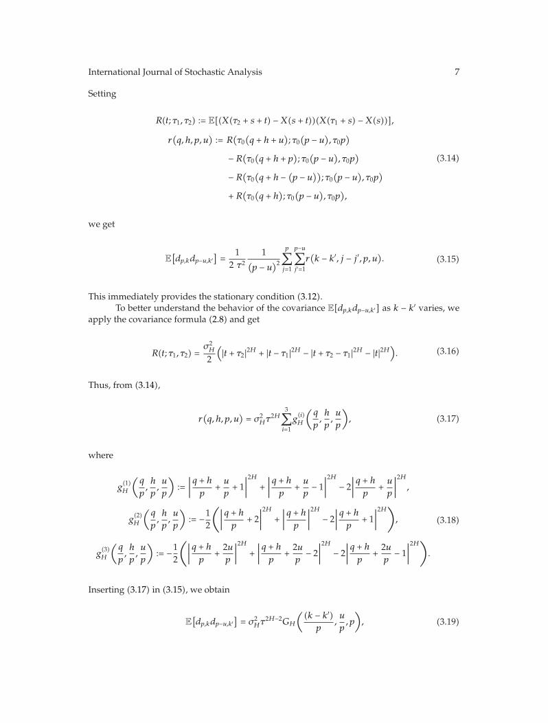
Setting
R(t; τ1, τ2) := E[(X(τ2 + s + t) −X(s + t))(X(τ1 + s) −X(s))],
r(q, h, p, u
):= R
(τ0(q + h + u
); τ0(p − u), τ0p
)
− R(τ0(q + h + p
); τ0(p − u), τ0p
)
− R(τ0(q + h − (p − u)); τ0
(p − u), τ0p
)
+ R(τ0(q + h
); τ0(p − u), τ0p
),
(3.14)
we get
E[dp,kdp−u,k′
]=
12 τ2
1(p − u)2
p∑j=1
p−u∑j ′=1
r(k − k′, j − j ′, p, u). (3.15)
This immediately provides the stationary condition (3.12).To better understand the behavior of the covariance E[dp,kdp−u,k′] as k − k′ varies, we
apply the covariance formula (2.8) and get
R(t; τ1, τ2) =σ2H
2
(|t + τ2|2H + |t − τ1|2H − |t + τ2 − τ1|2H − |t|2H
). (3.16)
Thus, from (3.14),
r(q, h, p, u
)= σ2
Hτ2H
3∑i=1
g(i)H
(q
p,h
p,u
p
), (3.17)
where
g(1)H
(q
p,h
p,u
p
):=∣∣∣∣q + hp
+u
p+ 1∣∣∣∣2H
+∣∣∣∣q + hp
+u
p− 1∣∣∣∣2H
− 2∣∣∣∣q + hp
+u
p
∣∣∣∣2H
,
g(2)H
(q
p,h
p,u
p
):= −1
2
(∣∣∣∣q + hp
+ 2∣∣∣∣2H
+∣∣∣∣q + hp
∣∣∣∣2H
− 2∣∣∣∣q + hp
+ 1∣∣∣∣2H),
g(3)H
(q
p,h
p,u
p
):= −1
2
(∣∣∣∣q + hp
+2up
∣∣∣∣2H
+∣∣∣∣q + hp
+2up
− 2∣∣∣∣2H
− 2∣∣∣∣q + hp
+2up
− 1∣∣∣∣2H).
(3.18)
Inserting (3.17) in (3.15), we obtain
E[dp,kdp−u,k′
]= σ2
Hτ2H−2GH
((k − k′)
p,u
p, p
), (3.19)
8 International Journal of Stochastic Analysis
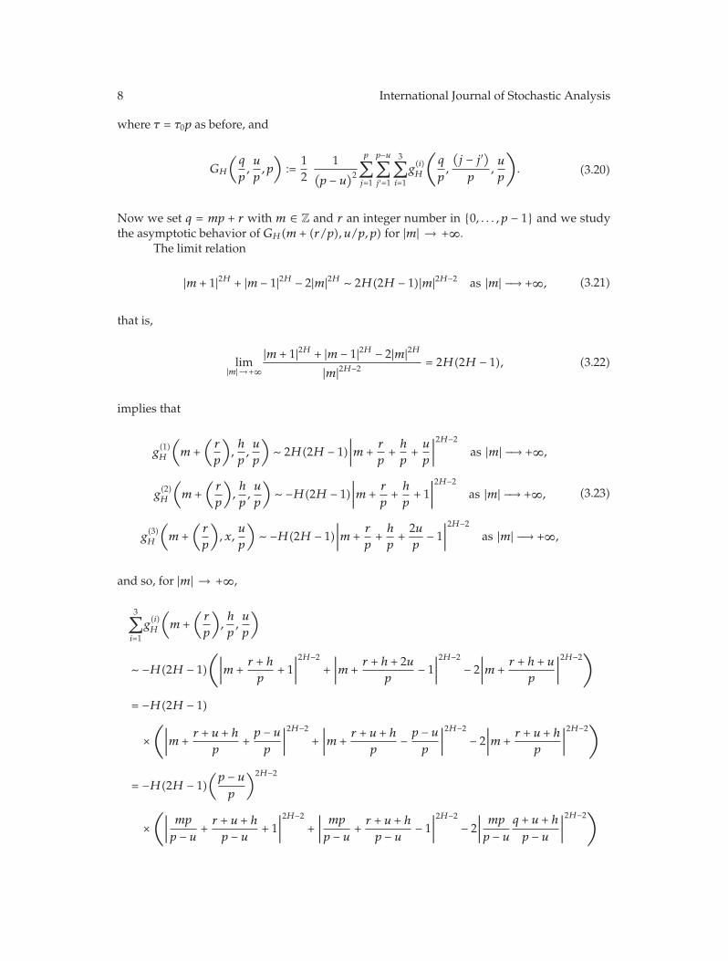
where τ = τ0p as before, and
GH
(q
p,u
p, p
):=
12
1(p − u)2
p∑j=1
p−u∑j ′=1
3∑i=1
g(i)H
(q
p,
(j − j ′)
p,u
p
). (3.20)
Now we set q = mp + r with m ∈ Z and r an integer number in {0, . . . , p − 1} and we studythe asymptotic behavior of GH(m + (r/p), u/p, p) for |m| → +∞.
The limit relation
|m + 1|2H + |m − 1|2H − 2|m|2H ∼ 2H(2H − 1)|m|2H−2 as |m| −→ +∞, (3.21)
that is,
lim|m|→+∞
|m + 1|2H + |m − 1|2H − 2|m|2H|m|2H−2 = 2H(2H − 1), (3.22)
implies that
g(1)H
(m +
(r
p
),h
p,u
p
)∼ 2H(2H − 1)
∣∣∣∣m +r
p+h
p+u
p
∣∣∣∣2H−2
as |m| −→ +∞,
g(2)H
(m +
(r
p
),h
p,u
p
)∼ −H(2H − 1)
∣∣∣∣m +r
p+h
p+ 1∣∣∣∣2H−2
as |m| −→ +∞,
g(3)H
(m +
(r
p
), x,
u
p
)∼ −H(2H − 1)
∣∣∣∣m +r
p+h
p+2up
− 1∣∣∣∣2H−2
as |m| −→ +∞,
(3.23)
and so, for |m| → +∞,
3∑i=1
g(i)H
(m +
(r
p
),h
p,u
p
)
∼ −H(2H − 1)
(∣∣∣∣m +r + hp
+ 1∣∣∣∣2H−2
+∣∣∣∣m +
r + h + 2up
− 1∣∣∣∣2H−2
− 2∣∣∣∣m +
r + h + up
∣∣∣∣2H−2)
= −H(2H − 1)
×(∣∣∣∣m +
r + u + hp
+p − up
∣∣∣∣2H−2
+∣∣∣∣m +
r + u + hp
− p − up
∣∣∣∣2H−2
− 2∣∣∣∣m +
r + u + hp
∣∣∣∣2H−2)
= −H(2H − 1)(p − up
)2H−2
×(∣∣∣∣
mp
p − u +r + u + hp − u + 1
∣∣∣∣2H−2
+∣∣∣∣mp
p − u +r + u + hp − u − 1
∣∣∣∣2H−2
− 2∣∣∣∣mp
p − uq + u + hp − u
∣∣∣∣2H−2)
International Journal of Stochastic Analysis 9
∼ cH(p − up
)2H−2∣∣∣∣mp
p − u +r + u + hp − u
∣∣∣∣2H−4
= cH(p − up
)2∣∣∣∣m +r + u + h
p
∣∣∣∣2H−4
∼ cH(p − up
)2
|m|2H−4,
(3.24)
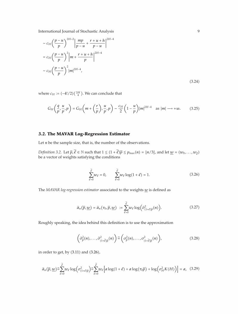
where cH := (−4!/2)( 2H4). We can conclude that
GH
(q
p,u
p, p
)= GH
(m +
(r
p
),u
p, p
)∼ cH
2
(1 − u
p
)|m|2H−4 as |m| −→ +∞. (3.25)
3.2. The MAVAR Log-Regression Estimator
Let n be the sample size, that is, the number of the observations.
Definition 3.2. Let p, � ∈ N such that 1 ≤ (1 + �)p ≤ pmax(n) = n/3�, and let w = (w0, . . . , w�)be a vector of weights satisfying the conditions
�∑�=0
w� = 0,�∑�=0
w� log(1 + �) = 1. (3.26)
TheMAVAR log-regression estimator associated to the weights w is defined as
αn(p,w)= αn
(τ0, p,w
):=
�∑�=0
w� log(σ2(1+�)p(n)
). (3.27)
Roughly speaking, the idea behind this definition is to use the approximation
(σ2p(n), . . . , σ
2(1+�)p
(n))=(σ2p(n), . . . , σ
2(1+�)p
(n)), (3.28)
in order to get, by (3.11) and (3.26),
αn(p,w)=
�∑�=0
w� log(σ2(1+�)p
)=
�∑�=0
w�
[α log(1 + �) + α log
(τ0p)+ log
(σ2HK(H)
)]= α, (3.29)
10 International Journal of Stochastic Analysis
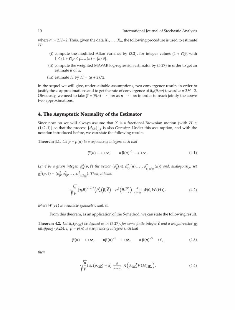
where α := 2H−2. Thus, given the dataX1, . . . , Xn, the following procedure is used to estimateH:
(i) compute the modified Allan variance by (3.2), for integer values (1 + �)p, with1 ≤ (1 + �)p ≤ pmax(n) = n/3�;
(ii) compute the weighted MAVAR log-regression estimator by (3.27) in order to get anestimate α of α;
(iii) estimateH by H = (α + 2)/2.
In the sequel we will give, under suitable assumptions, two convergence results in order tojustify these approximations and to get the rate of convergence of αn(p,w) toward α = 2H−2.Obviously, we need to take p = p(n) → +∞ as n → +∞ in order to reach jointly the abovetwo approximations.
4. The Asymptotic Normality of the Estimator
Since now on we will always assume that X is a fractional Brownian motion (with H ∈(1/2, 1)) so that the process {dp,k}p,k is also Gaussian. Under this assumption, and with thenotation introduced before, we can state the following results.
Theorem 4.1. Let p = p(n) be a sequence of integers such that
p(n) −→ +∞, n p(n)−1 −→ +∞. (4.1)
Let � be a given integer, σ2n(p, �) the vector (σ2
p(n), σ2
2p(n), . . . , σ2(1+�)p
(n)) and, analogously, set
σ2(p, �) = (σ2p, σ2
2p, . . . , σ2(1+�)p
). Then, it holds
√n
p
(τ0p)2−2H(
σ2n
(p, �)− σ2(p, �))
d−−−−→n→∞
N(0,W(H)), (4.2)
whereW(H) is a suitable symmetric matrix.
From this theorem, as an application of the δ-method, we can state the following result.
Theorem 4.2. Let αn(p,w) be defined as in (3.27), for some finite integer � and a weight-vector wsatisfying (3.26). If p = p(n) is a sequence of integers such that
p(n) −→ +∞, np(n)−1 −→ +∞, n p(n)−3 −→ 0, (4.3)
then
√n
p
(αn(p,w) − α) d−−−−→
n→∞N(0, wT
∗V (H)w∗), (4.4)
International Journal of Stochastic Analysis 11
where α = 2H − 2, the column-vector w∗ is such that [w∗]� := w�(1 + �)2−2H , and V (H) =(σ2
HK(H))−2W(H).
Let us stress that from the above result, and due to the condition np(n)−1 → +∞, itfollows that the estimator αn(p,w) is consistent.
Before starting the proof of the above theorems, we need the following lemma.
Lemma 4.3. Let p = p(n) be a sequence of integers such that
p(n) −→ +∞, np(n)−1 −→ +∞. (4.5)
For two given integers �′, �, with 0 ≤ �′ ≤ �, set p�′ = (�′ + 1)p and p� = (� + 1)p. Then
n
p
(τ0p)4−4H Cov
(σ2p� (n), σ
2p�′ (n)
)−−−−−→n→+∞
W�′,�(H), (4.6)
whereW�′,�(H) is a finite quantity.
Proof . Since n/p → +∞, without loss of generality we can assume that (1 + �)p ≤ pmax(n) =n/3� for each n. Recall the notation np = n − 3p + 1, and set n� = np� ∼ n and n�′ = np�′ ∼ n.From the definition of theMAVAR estimator and applying theWick’s rule for jointly Gaussianrandom variables (see the Appendix), we get
Cov(σ2p� (n), σ
2p�′ (n)
)=
1n�n�′
n�−1∑k=0
n�′ −1∑k′=0
Cov(d2p� ,k
, d2p�′ ,k′
)
=2
n�n�′
n�−1∑k=0
n�′ −1∑k′=0
Cov(dp�,k, dp�′ ,k′
)2
= 2σ4H(1 + �)4H−4
(τ0p)4H−4
n�n�′
n�−1∑k=0
n�′ −1∑k′=0
G2H
(k − k′
p�,u�′�p�
, p�
),
(4.7)
where u�′� = p�−p�′ . Since, by (3.20), the functionGH(q/p�, u�′�/p�, p�) only depends on q/p�and u�′�/p� = (� − �′)/(1 + �) as n → +∞, we rewrite the last line as
2σ4H(1 + �)4H−4
(τ0p)4H−4
n�n�′
n�−1∑k=0
n�′ −1∑k′=0
G2H
(k − k′
p�,(� − �′)1 + �
). (4.8)
This term, multiplied by (n/p)(τ0p)4−4H , is equal to
2σ4H(1 + �)4H−4 1
p
n
n�n�′
n�−1∑k=0
n�′ −1∑k′=0
G2H
(k − k′
p�,(� − �′)(1 + �)
). (4.9)
12 International Journal of Stochastic Analysis
It is easy to see that this quantity converges (to a finite strictly positive limit) if and only if
1p�
[n/p�]∑m=0
p�−1∑r=0
G2H
(m +
(r
p�
),(� − �′)(1 + �)
)(4.10)
converges. From (3.25) it holds
G2H
(m +
(r
p�
),(� − �′)(1 + �)
)∼ c2H
4
(1 − � − �′
1 + �
)2
m4H−8 as m −→ +∞. (4.11)
Thus, the quantity (4.10) is controlled in the limit n → ∞ by the sum∑∞
m=1m4H−8 that is
convergent.
Proof of Theorem 4.1. As before, without loss of generality, we can assume that (1 + �)p ≤pmax(n) for each n. Moreover, set again n� = np� and n�′ = np�′ . For a given real vectorvT = (v0, . . . , v�), let us consider the random variable Tn = T(p(n), �, v) defined as a linearcombination of the empirical variances σ2
p(n), . . . , σ2
(1+�)p(n) as follows:
Tn :=�∑�=0
v� σ2(1+�)p(n) =
�∑�=0
v�n�
n�−1∑k=0
d2(1+�)p,k. (4.12)
In order to prove the convergence stated in Theorem 4.1, we have to show that the random
variable√n/p (τ0p)
2−2H (Tn −∑�
�=0 v�σ2(1+�)p) converges to the normal distribution with zero
mean and variance vTW(H)v. To this purpose, we note that
√n
p
(τ0p)2−2H
⎛⎝Tn −
�∑�=0
v�σ2(1+�)p
⎞⎠ = V T
n AnVn − E
[V Tn AnVn
], (4.13)
where Vn is the random vector with entries d(1+�)p,k, for 0 ≤ � ≤ � and 0 ≤ k ≤ n� − 1, and An
is the diagonal matrix with entries
[An]((1+�)p,k),((1+�)p,k) =v�n�
√n
p
(τ0p)2−2H = O
((p)3/2−2H
n−1/2). (4.14)
By Lemma 4.3, ifW(H) is the symmetric matrix with [W(H)]�′,� =W�′,� when 0 ≤ �′ ≤ � ≤ �,it holds
Var[V Tn AnVn
]=n
p
(τ0p)4−4H �∑
�=0
�∑�′=0
v�v�′Cov(σ2(1+�)p(n), σ
2p(1+�′)(n)
)
−−−−−→n→+∞
�∑�=0
�∑�′=0
v�v�′W�′,�(H) = vTW(H)v,
(4.15)
therefore, condition (1) of Lemma A.2 is satisfied.
International Journal of Stochastic Analysis 13
In order to verify condition (2) of Lemma A.2, let Cn denote the covariance matrix ofthe random vector Vn, and let ρ[Cn] denote its spectral radius. By Lemma A.3, we have
ρ[Cn] ≤�∑�=0
ρ[Cn
((1 + �)p
)], (4.16)
where Cn((1 + �)p) is the covariance matrix of the subvector (d(1+�)p,k)k=0,...,n�−1. Applying thespectral radius estimate (A.3), and from equality (3.19), we then have
ρ[Cn
((1 + �)p
)] ≤ σ2H
[τ0(1 + �)p
]2H−2⎡⎣GH
(0, 0, p�
)+ 2
n�−1∑q=1
GH
(q
p�, 0, p�
)⎤⎦
= O((p)2H−1)
.
(4.17)
In order to conclude, it is enough to note that
ρ[An]ρ[Cn] = O((p)3/2−2H
n−1/2)O((p)2H−1) = O
((p)1/2
n−1/2)−−−−−→n→∞
0. (4.18)
Proof of Theorem 4.2. By assumptions (4.3) on the sequence p = p(n), and in particular fromthe condition n/(p)3 → 0, and inequality (3.11), it holds
√n
p
(τ0p)2−2H∣∣∣σ2
(1+�)p − σ2H
[τ0(1 + �)p
]2H−2K(H)
∣∣∣
≤ σ2H(1 + �)2H−2O
(n1/2(p)−3/2) −−−−−→
n→+∞0.
(4.19)
Thus, from Theorem 4.1, we get
√n
p
[(τ0p)2−2H
σ2n
(p, �)− σ2
∗]
d−−−−→n→∞
N(0,W(H)), (4.20)
where σ2∗ is the vector with elements
[σ2∗]�:= σ2
H(1 + �)2H−2K(H) for 0 ≤ � ≤ �. (4.21)
Now we observe that if f(x) :=∑�
�=0w� log(x�), then, by (3.26) and (3.27), we have
αn(p,w)= f(σ2(p, �))
= f((τ0p)2−2H
σ2(p, �)). (4.22)
14 International Journal of Stochastic Analysis
Moreover, α = f(σ2∗) and ∇f(σ2
∗) = (σ2HK(H))−1w∗. Therefore, by the application of the δ-
method, the convergence (4.20) entails
√n
p
(αn(p,w) − α) d−−−−→
n→∞N(0,∇f
(σ2∗)TW(H)∇f
(σ2∗))
, (4.23)
where
∇f(σ2∗)TW(H)∇f
(σ2∗)= wT
∗V (H)w∗, (4.24)
and thus concludes the proof.
Remark 4.4. By Lemma 4.3, and since by definition V�′,�(H) = (σ2HK(H))−2W�′,�(H), an
estimate of V�′,�(H), with 0 ≤ �′ ≤ � ≤ �, is given by
n
p
(τ0p)4−4H
σ4HK(H)2
Cov(σ2p� (n), σ
2p�′ (n)
). (4.25)
Therefore, setting ρ2n(w,H) equal to the corresponding estimate of wT∗V (H)w∗ divided by
n/p, that is
ρ2n(w,H
)=
2
K(H)2
�∑�=0
�∑�′=0
(1 + � ∧ �′1 + � ∨ �′
)2−2Hw�w�′
n�n�′
×n�∨�′ −1∑k=0
n�∧�′ −1∑k′=0
G2H
(k − k′
p(1 + � ∨ �′) ,|� − �′|
1 + � ∨ �′ , p(1 + � ∨ �′)
),
(4.26)
and from (4.6), we obtain the convergence
ρ−1n(w,H
)(αn(p,w) − α) d−−−−→
n→∞N(0, 1), (4.27)
which can be used to obtain an asymptotic confidence interval for the parameterH.
4.1. An Alternative Representation of the Covariance
It is well known that an FBM (with X(0) = 0 and E[X2(1)] = σ2H) has the following stochastic
integral representation (see [2, 16]):
X(t) =1
Γ(H + 1/2)
∫
R
{[(t − s)+]H−1/2 − (s−)H−1/2}
dWs. (4.28)
International Journal of Stochastic Analysis 15
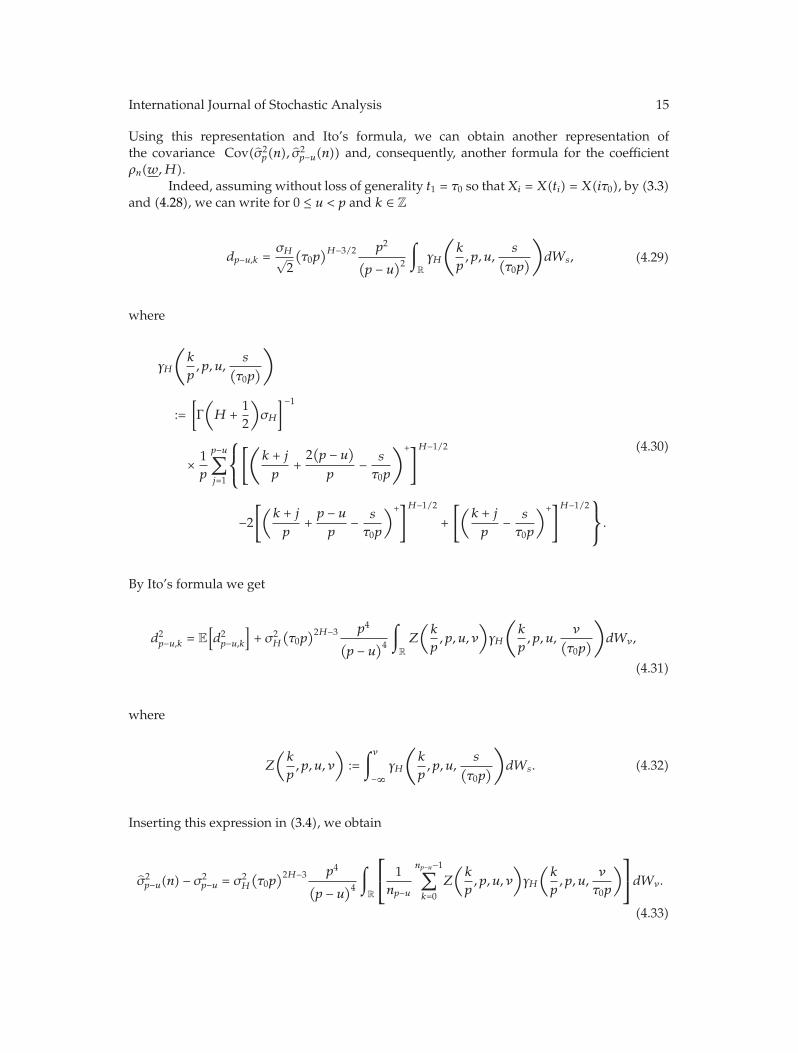
Using this representation and Ito’s formula, we can obtain another representation ofthe covariance Cov(σ2
p(n), σ2p−u(n)) and, consequently, another formula for the coefficient
ρn(w,H).Indeed, assuming without loss of generality t1 = τ0 so thatXi = X(ti) = X(iτ0), by (3.3)
and (4.28), we can write for 0 ≤ u < p and k ∈ Z
dp−u,k =σH√2
(τ0p)H−3/2 p2
(p − u)2
∫
R
γH
(k
p, p, u,
s(τ0p))dWs, (4.29)
where
γH
(k
p, p, u,
s(τ0p))
:=[Γ(H +
12
)σH
]−1
× 1p
p−u∑j=1
⎧⎨⎩
[(k + jp
+2(p − u)
p− s
τ0p
)+]H−1/2
−2[(
k + jp
+p − up
− s
τ0p
)+]H−1/2
+
[(k + jp
− s
τ0p
)+]H−1/2⎫⎬
⎭.
(4.30)
By Ito’s formula we get
d2p−u,k = E
[d2p−u,k]+ σ2
H
(τ0p)2H−3 p4
(p − u)4
∫
R
Z
(k
p, p, u, ν
)γH
(k
p, p, u,
ν(τ0p))dWν,
(4.31)
where
Z
(k
p, p, u, ν
):=∫ν−∞
γH
(k
p, p, u,
s(τ0p))dWs. (4.32)
Inserting this expression in (3.4), we obtain
σ2p−u(n) − σ2
p−u = σ2H
(τ0p)2H−3 p4
(p − u)4
∫
R
⎡⎣ 1np−u
np−u−1∑k=0
Z
(k
p, p, u, ν
)γH
(k
p, p, u,
ν
τ0p
)⎤⎦dWν.
(4.33)
16 International Journal of Stochastic Analysis
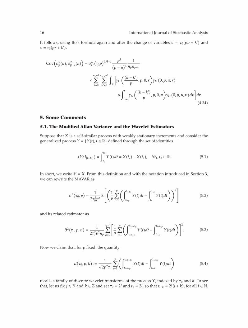
It follows, using Ito’s formula again and after the change of variables s = τ0(pv + k′) andν = τ0(pr + k′),
Cov(σ2p(n), σ
2p−u(n)
)= σ4
H
(τ0p)4H−4 p4
(p − u)4
1npnp−u
×np−1∑k=0
np−u−1∑k′=0
∫
R
[γH
((k − k′)
p, p, 0, r
)γH(0, p, u, r
)
×∫ r−∞
γH
((k − k′)
p, p, 0, v
)γH(0, p, u, v
)dv
]dr.
(4.34)
5. Some Comments
5.1. The Modified Allan Variance and the Wavelet Estimators
Suppose that X is a self-similar process with weakly stationary increments and consider thegeneralized process Y = {Y (t), t ∈ R} defined through the set of identities
⟨Y ; I[t1,t2]
⟩=∫ t2t1
Y (t)dt = X(t2) −X(t1), ∀t1, t2 ∈ R. (5.1)
In short, we write Y = X. From this definition and with the notation introduced in Section 3,we can rewrite the MAVAR as
σ2(τ0, p)=
12τ20p
2E
⎡⎣(
1p
p∑i=1
(∫ ti+2pti+p
Y (t)dt −∫ ti+pti
Y (t)dt
))2⎤⎦ (5.2)
and its related estimator as
σ2(τ0, p, n)=
12τ20p
2np
np−1∑k=0
[1p
p∑i=1
(∫ ti+k+2pti+k+p
Y (t)dt −∫ ti+k+pti+k
Y (t)dt
)]2. (5.3)
Now we claim that, for p fixed, the quantity
d(τ0, p, k
):=
1√2p2τ0
p∑i=1
(∫ ti+k+2pti+k+p
Y (t)dt −∫ ti+k+pti+k
Y (t)dt
)(5.4)
recalls a family of discrete wavelet transforms of the process Y , indexed by τ0 and k. To seethat, let us fix j ∈ N and k ∈ Z and set τ0 = 2j and t1 = 2j , so that ti+k = 2j(i + k), for all i ∈ N.
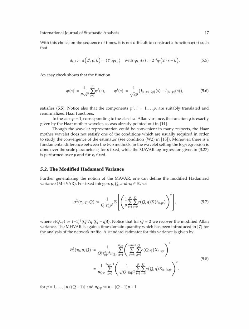
International Journal of Stochastic Analysis 17
With this choice on the sequence of times, it is not difficult to construct a function ψ(s) suchthat
dk,j := d(2j , p, k
)=⟨Y ;ψk,j
⟩with ψk,j(s) := 2−jψ
(2−js − k
). (5.5)
An easy check shows that the function
ψ(s) :=1
p√p
p∑i=1
ψi(s), ψi(s) :=1√2p
(I[i+p,i+2p](s) − I[i,i+p](s)
), (5.6)
satisfies (5.5). Notice also that the components ψi, i = 1, . . . p, are suitably translated andrenormalized Haar functions.
In the case p = 1, corresponding to the classical Allan variance, the function ψ is exactlygiven by the Haar mother wavelet, as was already pointed out in [14].
Though the wavelet representation could be convenient in many respects, the Haarmother wavelet does not satisfy one of the conditions which are usually required in orderto study the convergence of the estimator (see condition (W2) in [18]). Moreover, there is afundamental difference between the two methods: in the wavelet setting the log-regression isdone over the scale parameter τ0 for p fixed, while the MAVAR log-regression given in (3.27)is performed over p and for τ0 fixed.
5.2. The Modified Hadamard Variance
Further generalizing the notion of the MAVAR, one can define the modified Hadamardvariance (MHVAR). For fixed integers p,Q, and τ0 ∈ R, set
σ2(τ0, p,Q):=
1Q!τ20p
2E
⎡⎢⎣⎛⎝1p
p∑i=1
Q∑q=0
c(Q, q)X(ti+qp)⎞⎠
2⎤⎥⎦, (5.7)
where c(Q, q) := (−1)q(Q!/q!(Q − q)!). Notice that for Q = 2 we recover the modified Allanvariance. The MHVAR is again a time-domain quantity which has been introduced in [7] forthe analysis of the network traffic. A standard estimator for this variance is given by
σ2n
(τ0, p,Q
):=
1Q!τ20p
4nQ,p
nQ,p∑h=1
⎛⎝
p+h−1∑i′=h
Q∑q=0
c(Q, q)Xi′+qp
⎞⎠
2
=1
nQ,p
nQ,p−1∑k=0
⎛⎝ 1√
Q!τ0p2
p∑i=1
Q∑q=0
c(Q, q)Xk+i+qp
⎞⎠
2
,
(5.8)
for p = 1, . . . , [n/(Q + 1)] and nQ,p := n − (Q + 1)p + 1.
18 International Journal of Stochastic Analysis
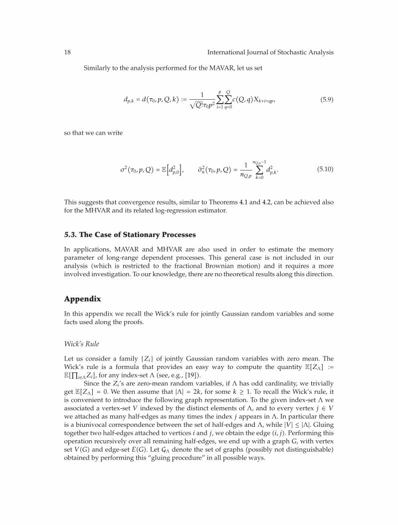
Similarly to the analysis performed for the MAVAR, let us set
dp,k = d(τ0, p,Q, k
):=
1√Q!τ0p2
p∑i=1
Q∑q=0
c(Q, q)Xk+i+qp, (5.9)
so that we can write
σ2(τ0, p,Q)= E
[d2p,0
], σ2
n
(τ0, p,Q
)=
1nQ,p
nQ,p−1∑k=0
d2p,k. (5.10)
This suggests that convergence results, similar to Theorems 4.1 and 4.2, can be achieved alsofor the MHVAR and its related log-regression estimator.
5.3. The Case of Stationary Processes
In applications, MAVAR and MHVAR are also used in order to estimate the memoryparameter of long-range dependent processes. This general case is not included in ouranalysis (which is restricted to the fractional Brownian motion) and it requires a moreinvolved investigation. To our knowledge, there are no theoretical results along this direction.
Appendix
In this appendix we recall the Wick’s rule for jointly Gaussian random variables and somefacts used along the proofs.
Wick’s Rule
Let us consider a family {Zi} of jointly Gaussian random variables with zero mean. TheWick’s rule is a formula that provides an easy way to compute the quantity E[ZΛ] :=E[∏
i∈ΛZi], for any index-set Λ (see, e.g., [19]).Since the Zi’s are zero-mean random variables, if Λ has odd cardinality, we trivially
get E[ZΛ] = 0. We then assume that |Λ| = 2k, for some k ≥ 1. To recall the Wick’s rule, itis convenient to introduce the following graph representation. To the given index-set Λ weassociated a vertex-set V indexed by the distinct elements of Λ, and to every vertex j ∈ Vwe attached as many half-edges as many times the index j appears in Λ. In particular thereis a biunivocal correspondence between the set of half-edges and Λ, while |V | ≤ |Λ|. Gluingtogether two half-edges attached to vertices i and j, we obtain the edge (i, j). Performing thisoperation recursively over all remaining half-edges, we end up with a graph G, with vertexset V (G) and edge-set E(G). Let GΛ denote the set of graphs (possibly not distinguishable)obtained by performing this “gluing procedure” in all possible ways.
International Journal of Stochastic Analysis 19
With this notation, and for all index-sets Λ with even cardinality, the Wick’s rule for afamily {Zi} of jointly centered Gaussian random variables provides the identity
E[ZΛ] =∑G∈GΛ
∏(i,j)∈E(G)
E[ZiZj
]. (A.1)
Example A.1. Consider the quantity E[Z2kZ
2j ], for j /= k. By the graphical representation, we
take a vertex set V = {j, k} with two half-edges attached to each vertex and perform thegluing operation on the half-edges. We then obtain the following three graphs (identified bytheir edges):G1 = (j, k)(j, k),G2 = (j, k)(j, k), and G3 = (j, j)(k, k). Thus, from theWick’s rule,we get the identity
E
[Z2kZ
2j
]= 2E
[ZjZk
]2 + E
[Z2j
]E
[Z2k
], (A.2)
that has been used throughout the paper.
Now we recall some facts used in the proof of Theorem 4.1.Denote by ρ[A] the spectral radius of a matrix A = {ai,j}1≤i,j≤n, then
ρ[A] ≤ max1≤j≤n
n∑i=1
∣∣ai,j∣∣. (A.3)
Moreover the following lemmas hold.
Lemma A.2 (see [13]). Let (Vn) be a sequence of centered Gaussian random vectors and denote byCn the covariance matrix of Vn. Let (An) be a sequence of deterministic symmetric matrices such that
(1) limn→+∞ Var[V Tn AnVn] = λ2 ∈ [0,+∞),
(2) limn→+∞ρ[An]ρ[Cn] = 0.
Then V Tn AnVn − E[V T
n AnVn] converges in distribution to the normal law N(0, λ2).
Lemma A.3 (see [11]). Letm ≥ 2 be an integer and C am×m covariance matrix. Let r be an integersuch that 1 ≤ r ≤ m − 1. Denote by C1 the top left submatrix with size r × r and by C2 the bottomright submatrix with size (m − r) × (m − r), that is,
C1 =[Ci,j
]1≤i,j≤r , C2 =
[Ci,j
]r+1≤i,j≤m. (A.4)
Then ρ[C] ≤ ρ[C1] + ρ[C2].
Acknowledgments
The authors are grateful to Stefano Bregni for having introduced them to this subject,proposing open questions and providing useful insights. They are also grateful to MarcoFerrari for a helpful remark on the first version of this work. This work was partiallysupported by GNAMPA (2011).
20 International Journal of Stochastic Analysis
References
[1] J. Beran, Statistics for Long-Memory Processes, vol. 61 of Monographs on Statistics and Applied Probability,Chapman and Hall, London, UK, 1994.
[2] B. B. Mandelbrot and J. W. Van Ness, “Fractional Brownian motions, fractional noises andapplications,” SIAM Review, vol. 10, pp. 422–437, 1968.
[3] L. G. Bernier, “Theoretical analysis of the modified Allan variance,” in Proceedings of the 41st AnnualFrequency Control Symposium, pp. 161–121, 1987.
[4] S. Bergni, “Characterization andmodelling of clocks,” in Synchronization of Digital Telecommu-NicationsNetworks, John Wiley & Sons, 2002.
[5] S. Bregni and L. Primerano, “The modified Allan variance as time-domain analysis tool for estimatingthe hurst parameter of long-range dependent traffic,” in IEEE Global Telecommunications Conference(GLOBECOM ’04), pp. 1406–1410, December 2004.
[6] S. Bregni and W. Erangoli, “Fractional noise in experimental measurements of IP traffic ina metropolitan area network,” in Proceedings of the IEEE Global Telecommunications Conference(GLOBECOM ’05), pp. 781–785, December 2005.
[7] S. Bregni and L. Jmoda, “Accurate estimation of the Hurst parameter of long-range dependent trafficusing modified Allan and Hadamard variances,” IEEE Transactions on Communications, vol. 56, no. 11,pp. 1900–1906, 2008.
[8] A. Bianchi, S. Bregni, I. Crimaldi, and M. FERRARI, “Analysis of a hurst parameter estimator basedon the modified Allan variance,” in Proceedings of the IEEE Global Telecommunications Conference andExhibition (GLOBECOM) and IEEE Xplore, 2012.
[9] J. F. Coeurjolly, “Simulation and identification of the fractional brownian motion: a bibliographicaland comparative study,” Journal of Statistical Software, vol. 5, pp. 1–53, 2000.
[10] J.-F. Coeurjolly, “Estimating the parameters of a fractional Brownian motion by discrete variations ofits sample paths,” Statistical Inference for Stochastic Processes, vol. 4, no. 2, pp. 199–227, 2001.
[11] E. Moulines, F. Roueff, and M. S. Taqqu, “Central limit theorem for the log-regression waveletestimation of the memory parameter in the gaussian semi-parametric context,” Fractals, vol. 15, no. 4,pp. 301–313, 2007.
[12] E. Moulines, F. Roueff, and M. S. Taqqu, “On the spectral density of the wavelet coefficients of long-memory time series with application to the log-regression estimation of the memory parameter,”Journal of Time Series Analysis, vol. 28, no. 2, pp. 155–187, 2007.
[13] E. Moulines, F. Roueff, and M. S. Taqqu, “A wavelet whittle estimator of the memory parameter of anonstationary Gaussian time series,” Annals of Statistics, vol. 36, no. 4, pp. 1925–1956, 2008.
[14] P. Abry and D. Veitch, “Wavelet analysis of long-range-dependent traffic patrice abry and darrylveitch,” IEEE Transactions on Information Theory, vol. 44, no. 1, pp. 2–15, 1998.
[15] P. Abry, P. Flandrin, M. S. Taqqu, and D. Veitch, “Wavelets for the analysis, estimation and synthesisof scaling data,” in Self-Similar Network Traffic and Performance Evaluation, K. Park and W. Willinger,Eds., pp. 39–88, Wiley, New York, NY, USA, 2000.
[16] T. Lindstrom, “A weighted random walk approximation to fractional Brownian motion,” Tech. Rep.11, Department of Mathematics, University of Oslo, 2007, http://arxiv.org/abs/0708.1905.
[17] A. M. Yaglom, Correlation Theory of Stationary and Related Random Functions, Springer Series inStatistics, Springer, New York, NY, USA, 1987.
[18] F. Roueff and M. S. Taqqu, “Asymptotic normality of wavelet estimators of the memory parameterfor linear processes,” Journal of Time Series Analysis, vol. 30, no. 5, pp. 534–558, 2009.
[19] J. Glimm and A. Jaffe, Quantum Physics. A Functional Integral Point of View, Springer, New York, NY,USA, 2nd edition, 1987.

Submit your manuscripts athttp://www.hindawi.com
Hindawi Publishing Corporationhttp://www.hindawi.com Volume 2014
MathematicsJournal of
Hindawi Publishing Corporationhttp://www.hindawi.com Volume 2014
Mathematical Problems in Engineering
Hindawi Publishing Corporationhttp://www.hindawi.com
Differential EquationsInternational Journal of
Volume 2014
Applied MathematicsJournal of
Hindawi Publishing Corporationhttp://www.hindawi.com Volume 2014
Probability and StatisticsHindawi Publishing Corporationhttp://www.hindawi.com Volume 2014
Journal of
Hindawi Publishing Corporationhttp://www.hindawi.com Volume 2014
Mathematical PhysicsAdvances in
Complex AnalysisJournal of
Hindawi Publishing Corporationhttp://www.hindawi.com Volume 2014
OptimizationJournal of
Hindawi Publishing Corporationhttp://www.hindawi.com Volume 2014
CombinatoricsHindawi Publishing Corporationhttp://www.hindawi.com Volume 2014
International Journal of
Hindawi Publishing Corporationhttp://www.hindawi.com Volume 2014
Operations ResearchAdvances in
Journal of
Hindawi Publishing Corporationhttp://www.hindawi.com Volume 2014
Function Spaces
Abstract and Applied AnalysisHindawi Publishing Corporationhttp://www.hindawi.com Volume 2014
International Journal of Mathematics and Mathematical Sciences
Hindawi Publishing Corporationhttp://www.hindawi.com Volume 2014
The Scientific World JournalHindawi Publishing Corporation http://www.hindawi.com Volume 2014
Hindawi Publishing Corporationhttp://www.hindawi.com Volume 2014
Algebra
Discrete Dynamics in Nature and Society
Hindawi Publishing Corporationhttp://www.hindawi.com Volume 2014
Hindawi Publishing Corporationhttp://www.hindawi.com Volume 2014
Decision SciencesAdvances in
Discrete MathematicsJournal of
Hindawi Publishing Corporationhttp://www.hindawi.com
Volume 2014 Hindawi Publishing Corporationhttp://www.hindawi.com Volume 2014
Stochastic AnalysisInternational Journal of